FEDERAL REVENUE FORECASTING

Rudolph G. Penner Senior Fellow

The Urban Institute 2100 M St. NW

Washington, DC, 20037

Chapter reproduced with permission from Handbook of Government Budget Forecasting (New York: Taylor & Francis), forthcoming in July 2008.

Email: rpenner@ui.urban.org Phone: (202) 261-5212 Fax: (202) 728-0232

2

FEDERAL REVENUE FORECASTING

Rudolph G. Penner The Urban Institute

Federal revenue forecasts play an important role in shaping the national debate

over future spending and tax policy.1 Federal revenue forecasts are often very wrong.

That is not because the technicians making them are unskilled. In fact, they are generally

highly talented, dedicated civil servants. The basic problem is that revenue forecasting,

like hurricane forecasting or earthquake forecasting, is very difficult.

The forecasting process consists of many steps and errors are likely to occur in

each one. A series of small errors that happen to go in the same direction can make a

forecast look incompetent. Large errors that offset each other—even those that could

signal incompetence—can make a forecast look brilliant.

The Forecasting Process

I shall focus on the process as it exists at the Congressional Budget Office (CBO).

Technically, the approach is very similar at the U.S. Treasury, but occasionally, the

process in the Executive Branch is warped by political strategizing that differs from

administration to administration. I shall return to this topic later.

The CBO and the Executive Branch typically provide two forecasts per year. The

former usually reports to the Congress in January and August while the latter reports in

January or early February and in July. CBO’s January forecast is most important, because

1 The author would like to thank the Tax Policy Center of the Brookings Institution and the Urban Institute for financial support and Leonard Burman and Larry Ozanne for useful comments. The conclusions are the author’s own and should not be attributed to the Urban Institute, its trustees, or its funders.

2

3

the macroeconomic assumptions that it generates are used to derive the spending and

revenue baseline that will be used by Congress throughout the year. Those same

assumptions are often important in estimating the effect of tax policy changes on

revenues or program changes on outlays. The CBO has used a time horizon of ten years

for their economic and budget forecast in recent years, but the Congress most often uses a

time horizon of five years for formulating their budget resolution. The administration has

recently emphasized a five-year horizon, but provides some estimates for a 10-year

period.

All short-run revenue forecasts must begin with an economic forecast. CBO staff

carefully tracks the economy all year long, but the formal forecasting process for the

January report generally begins in the fall by examining the forecasts generated by

private forecasting companies, such as Macroeconomic Advisers. These forecasting

companies use macroeconomic models that assume that the structure of the economy is

constant. This assumption has been challenged by the so-called Lucas critique. Lucas

(1976) and other rational expectations theorists argue that the structure of the economy is

constantly evolving and attempts to estimate the parameters of equations that assume a

constant structure can lead to a meaningless result.

But traditional macro models have one huge advantage. They contain a number of

identities that must add up. For example, gross investment must equal gross domestic and

foreign saving plus a statistical discrepancy. There are definitional linkages between the

working age population, the labor force participation rate and employment plus

unemployment. The number of hours worked is linked to the gross domestic product

(GDP) through labor productivity. Such identities force the forecast to be logical.

3

4

Nonetheless, no one would blindly run a macro model and uncritically accept the

result. The analysis is almost always leavened by a large dose of judgment. For example,

a housing specialist may decide that the model’s forecast of residential investment is too

low. He or she can then modify the relevant equations to make it come out higher. But

this change will reverberate through the model’s definitional statements and may require

domestic saving to be higher than is reasonable. The analyst may then have to re-examine

his or her modifications to the model.

Other statistical approaches, such as vector autoregression or other types of time

series analysis, do not provide the same kind of logical check on judgmental adjustments

to a forecast. Consequently, old-fashioned macro models continue to play a very

important role in the forecasting process. Perhaps, one can interpret judgmental

adjustments to equations as a recognition that the structure of the economy is constantly

changing.

The short-run January forecast extends only to the end of the next calendar year.

That is to say, the January 1990 forecast extended through the period until the end of

calendar 1991. CBO calls its longer run estimates “projections.” It is explicitly noted that

there is no attempt to forecast the ups and downs of the business cycle in the longer run.

Instead, CBO puts much effort into deriving the GDP path that the economy would be on

with full employment. Defining “full employment” is no easy task, but CBO tries to

estimate the level of the unemployment rate that would be neither inflationary nor

deflationary. Much controversy surrounds such estimates. Having estimated the path

consistent with this unemployment rate, usually called the “potential GDP” path, it is

4

5

usually assumed that the economy will approach it between the end of the forecast period

and five years out.

The economic forecast initially focuses on the product side of the National

Income and Product Accounts (NIPA). That is to say, various types of consumption and

private investment are analyzed as well as exports, imports, and federal and state and

local government purchases. However, the product side of the accounts is of little help

when it comes to forecasting government revenue. For that, one has to forecast the

different types of income generated by the production of final goods and services.

Theoretically, the income side of the NIPA should exactly equal the product side.

However, no government statistician can measure either side with complete accuracy.

Consequently, there is always a statistical discrepancy that jumps around from year to

year. Usually, the product side exceeds the income side slightly and CBO assumes that

the statistical discrepancy will revert to its average over the period, 1950–2005, or to

about one percent of the product side. (CBO 2006) The assumed speed of the reversion

depends on how far recent statistical discrepancies diverge from the historical mean. In

2006, the income side of the accounts grew faster than the product side and the

discrepancy has been smaller than usual. Using the rule of thumb that the discrepancy

will return to its historical average will imply that revenues will grow more slowly than

the product side of the GDP unless there is also a change in the distribution of total

income among tax brackets that raises the average tax rate.

The need to project a statistical discrepancy is just one of many difficult

challenges facing revenue forecasters. It is like having to forecast a random number.

5

6

The largest share of total income goes to labor. The labor share tends to be nearly

constant over time, although it can deviate from its historical average in either direction

for several years in a row. The CBO assumption is that it will revert to its historical

mean. The labor share is then divided into components. The most important consists of

wages, salaries and supplements. Supplements include payroll taxes and the cost of

employee benefits such as health insurance. Total compensation is assumed to vary with

employment, productivity, and inflation. The revenue yield per dollar of compensation

clearly depends on how it is divided among wages, payroll taxes, and untaxed benefits.

The forecast of untaxed fringe benefits depends on, among other things, the rate

of health cost growth and rules governing pension contributions. Aggregate wages

depend on the forecast of hours worked and wage rates. The amount of income tax

revenue derived from wages depends upon their distribution among various tax brackets.

Withheld income taxes on wages are forecast separately from non-withheld estimated

taxes and taxes on self-employment income.

The forecast of Social Security payroll tax revenues depends on the forecast of

total wages and also on their distribution because of the ceiling applying to Social

Security payroll taxes. Payroll taxes for hospital insurance (Medicare) do not have a

ceiling. Social insurance taxes accounted for 37 percent of total revenues in 2005.

Proprietors’ income is estimated two ways. The first method measures it as a

residual. Wages, salaries and supplements are forecast as described above and subtracted

from labor’s overall share. It is assumed that 65 percent of proprietors’ income accrues to

labor; so the residual is divided by 0.65 to get total proprietors’ income. As a check on

this residual estimate, CBO analyzes recent trends from tax returns of farmers and

6

7

professionals, but the data are of low quality. There is much tax evasion in the sole

proprietor segment of the economy. The Bureau of Economic Analysis (BEA) assumes

that underreporting has equaled about 50 percent of non-farm proprietors’ income over

the past 10 years and has been as high as 70 percent. Low quality data and significant

revisions of historical data are common and often conspire to make life miserable for the

revenue forecaster.

After the wage share has been estimated, other income must be divided up into

capital’s share, the statistical discrepancy, surpluses less subsidies of government

enterprises, and taxes on production, such as sales taxes. Components other than the

capital share are forecast independently. Numerous components of the capital share are

also estimated independently. These include net income from abroad, depreciation,

interest payments, proprietors’ capital income and rents and royalties. Finally, corporate

profits are estimated as a residual. That estimate is checked against private forecasts and

sometimes altered. Then other components of income have to be adjusted upwards or

downwards to be sure that everything adds up.

The concept of profits that comes from this process is known as “economic

profits.” CBO must also estimate “taxable profits” that are more relevant for estimating

corporate tax receipts. To go from economic to taxable profits, they adjust for the

difference between economic depreciation and the depreciation allowed for tax purposes

and they add capital gains on inventories and other assets. Capital gains are not included

in income as measured by the NIPA. Numerous other adjustments are necessary in the

process of deriving taxable profits. Corporate tax receipts accounted for 13 percent of

total federal revenues in 2005 and are one of the most volatile revenue sources.

7

8

Because capital gains are not counted in NIPA’s definition of income, they must

be estimated separately in order to estimate capital gains tax revenues from individual

and corporate income tax returns. Capital gains are extremely volatile, but it is generally

assumed that they will revert to their historical mean as a ratio to GDP. The estimate of

realized capital gains can be affected by changes in tax policy. For example, it is assumed

that realized capital gains will rise following a rate cut. Or if rates are due to rise in the

future, as they did between 1986 and 1987, it is assumed that there will be a surge in

realizations just before the rate changes.

The individual income tax revenue yield per dollar of personal income depends

crucially on how that income is distributed. In recent years, the very rich have become

responsible for a higher share of individual income tax receipts in part because income

inequality has increased and in part because lower income groups have been taken off the

tax rolls by a number of legislative actions. In 1979, the top one percent of the income

distribution received 9.3 percent of income and paid 18.3 percent of individual tax

liabilities. In 2003, their share of income had risen to 14.3 percent and their share of

income tax liabilities to 34.6 percent. Because the share of the top group tends to be quite

volatile, growing income inequality has added to the difficulty of forecasting individual

income tax receipts. In 2000, the income share of the top one percent was 17.8 percent,

but it was only 13.5 percent by 2002 after the stock market bubble had burst. In 2003, it

again rose to 14.3 percent (CBO 2004).

8

9

The Forecasting Record

When actual revenues deviate from the total forecast, it can be for three reasons.

First, the economic forecast was wrong. (It always will be in its details.) Second,

technical factors may distort revenues. For example, forecasters may come close with

their macroeconomic forecast, but the revenue forecast may still go awry because income

has been incorrectly distributed among various tax brackets. Third, the Congress may

have changed the law. This analysis will focus on the sum of economic and technical

errors. It is not the responsibility of CBO forecasters to predict legislative actions. The

analysis will not explore the relationship between economic and technical errors. That

has been done by Kitchen (2003) who convincingly argues that a considerable portion of

technical errors can be explained by errors in the economic forecast.

The analysis will examine forecast errors using three time horizons. The first

looks at the errors in the forecast made early in the calendar year (usually January) for the

fiscal year ending at the end of the following September. That is to say, the error for

forecasts published when the fiscal year is already over three months old. The second

analyzes errors made early in the calendar year in forecasts for the next fiscal year. For

example, the analysis considers the error for fiscal 1985 made in the forecast in early

1984. The third examines errors for fiscal years five years into the future. For example,

the analysis discusses the accuracy of the forecast for fiscal 1989 made in the forecast of

early 1984.

9

10

CBO did not keep records of their errors on a consistent basis until after 1983 and

as this is written, the latest year for which data are available is 2005. That implies that we

must be satisfied with very small samples. The sample size is 22 for within fiscal year

forecasts and for forecasts one year out. For five-year forecasts the sample is only 17.

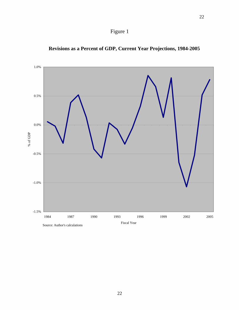
Errors Within the Fiscal Year—Figure 1 illustrates the forecast errors made early

in the calendar year for the fiscal year ending at the end of the following September. An

error with a positive value means that actual revenues exceeded forecast revenues while a

negative number means the reverse.

The average error for the 22-year period is only 0.1 percent of GDP, thus

confirming Auerbach’s (1999) conclusion that there is no significant positive or negative

bias in CBO revenue forecasting. The average absolute error is 0.4 percent of GDP, or

almost $50 billion at 2005 levels of GDP. Errors of this size can have important political

significance. There are few policy changes that would have that much impact on the

budget deficit over such a short period. The largest error occurred in 2002 when revenues

were overestimated by 1.1 percent of GDP or by $111 billion.

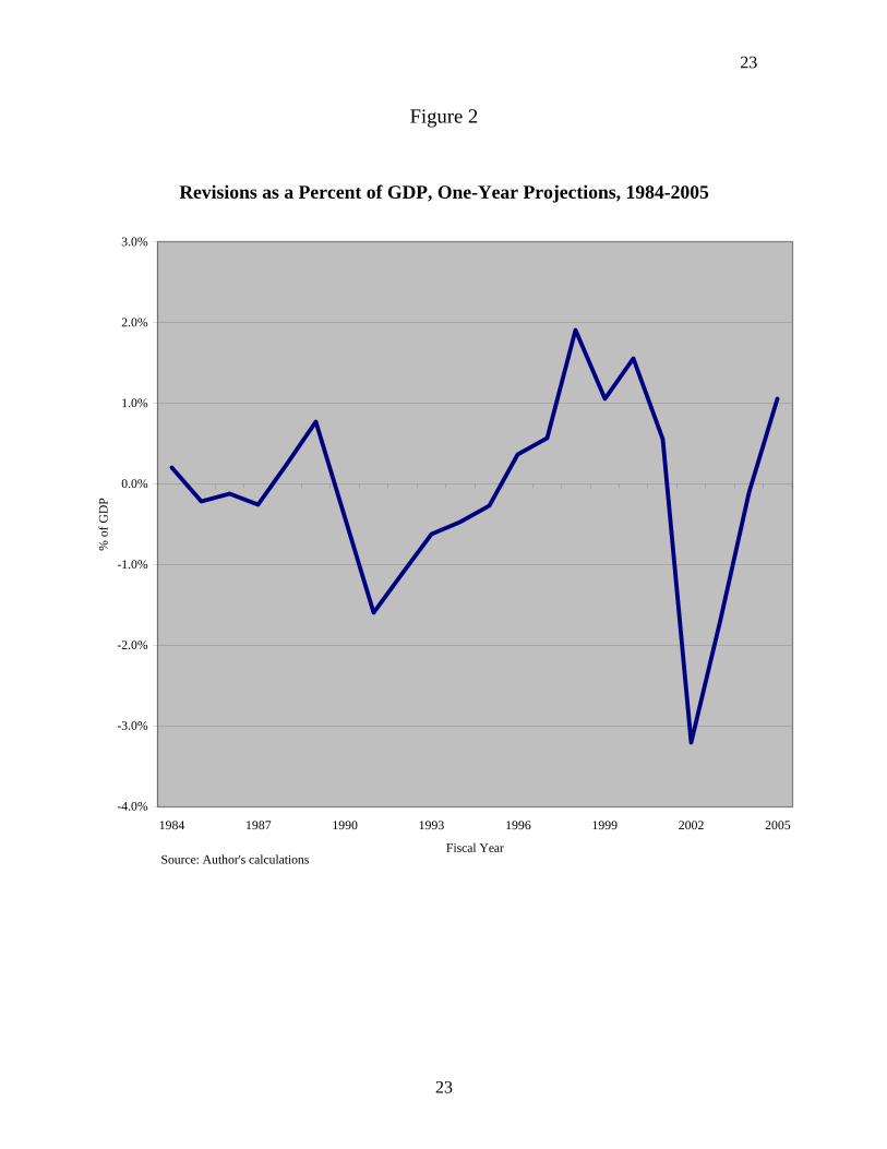
Errors for the Next Fiscal Year—The revenue forecast made in January for the

fiscal year starting the following September is the most important produced by CBO for it

will be used by the Congress for formulating the Budget Resolution for that fiscal year.

The errors in that forecast are shown in figure 2.

The average error is only -.001 percent of GDP. Obviously, there is no significant

upward or downward bias in CBO forecasting methods. The average absolute error was

0.8 percent of GDP or $98 billion at 2005 levels of GDP. Errors of this size indicate that

the Congress is often badly misled with regard to the fiscal outlook. It also implies that

10

11

the deficit outlook is almost always changed more by changes in the forecast than it is by

changes in policy.

It is for that reason that budget plans that attempt to hit a specific deficit target in

the future are almost certain to fail. Changes in policy cannot keep up with changes in the

forecast. This is the main reason for the failure of the Gramm-Rudman-Hollings

legislation that tried to target deficits in the last half of the 1980s.2

The largest revenue forecasting error was made in January of 2001 for fiscal year

2002. Revenues were overestimated by 3.2 percent of GDP or by $333 billion. It is

interesting to speculate whether the tax cut debate of 2001 would have been much

different had legislators known that revenues were about to crash. One would think that

the tax cut might have been more modest. On the other hand, a sizeable portion of the

revenue shortfall was caused by the unpredicted recession of 2001 and had the recession

been properly forecast it would have strengthened the case for tax cutting. The revenue

and deficit forecast had become much more dismal by 2003, but that did not deter the

Congress from passing large tax cuts on dividends and capital gains.

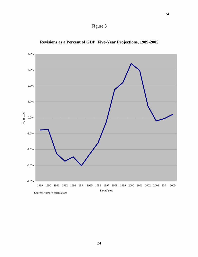
Errors in Five-Year Forecasts—As bad as the record is for forecasts with short

time horizons, it becomes very much worse when one goes out five years. The record is

revealed by figure 3. There is, however, no statistically significant bias as the average

error is only -.003 percent of GDP. The average absolute error is 1.6 percent of GDP or

$196 billion at 2005 levels of GDP. The largest error occurred for the year 2000 when

actual revenues exceeded the forecast made in 1995 by $330 billion or 3.4 percent of

2000 GDP.

2 Not everyone would characterize Gramm-Rudman-Hollings as a failure. See Gramlich (1990).

11

12

Curiously, the five-year forecasts for the years 2002 through 2005 appear to be

more accurate than the shorter run forecasts made for those years. However, one should

not believe that we have suddenly become better at long-term forecasting. In 1997, when

the 2002 forecast was formulated, it was recognized that revenues were coming in higher

than expected. Forecasts of short-run revenues were then moved upward more than those

of longer run revenues. Revenues then unexpectedly plummeted in the early years of the

century. Short-term forecasts were adjusted downward, but because the long-run forecast

had been kept relatively stable in the period of excess revenues, it looked pretty accurate

when revenues started to fall again.

The CBO extended their forecast horizon to 10 years starting in 1996. It is too

early to do any statistical analysis of 10-year forecast errors because the sample is too

small. But it is clear that budget projections for this time horizon have been wildly

misleading. For example, the projection of the budget balance for 2007, first made in

1997, had swung through a range of $801 billion by 2000. Because policy changes had

reduced the surplus in the interim, the implied economic and technical forecast error was

even greater—$844 billion or 6 percent of GDP. Future results may imply that was an

unusual aberration, but we do not know at this point and I would argue that 10-year

forecasts are far too unreliable to serve as a basis for formulating a budget resolution that

goes that far out.

That is because the Budget Resolution passed by the Congress contains very

precise targets for revenues, expenditures and deficits. Nevertheless, I believe that CBO

should continue to do 10-year forecasts, because they can be useful for other purposes.

For example, they are still useful for providing the economic assumptions used to

12

13

evaluate the costs or gains from changes in tax and spending policies. One can examine

these estimates for 10 years even if the Budget Resolution only covers five years.

Estimates of the effects of changes in policy are not as sensitive to errors in the economic

assumptions as is the estimate of future budget deficits.

The most important reason for extending the time horizon when policy changes

are considered is that their long-run effects may differ greatly from their short-run effects.

If the revenue loss associated with a particular tax cut grows rapidly through time, the

growing losses are likely to be revealed even if the economic assumptions used to

evaluate the tax change eventually turn out to have been overly optimistic or pessimistic.

That result cannot always be guaranteed, but it is true enough of the time to warrant

doing long-run estimates—in some cases, even for longer than ten years. Alternatively,

the present value of revenue losses or gains can be estimated for very long periods, but

not many laymen understand present values and a time profile of revenue changes may be

more useful.

Serial Correlation of Forecast Errors

A superficial look at figures 1, 2, and 3 suggests significant serial correlation in

the forecast errors. That is to say, if CBO makes an error in an overly optimistic or

pessimistic direction one year, it is highly probable that it will make an error in the same

direction the following year.

One indicator of serial correlation is the number of runs of positive and negative

errors in a time series. A large number of runs relative to the size of the sample indicates

a low serial correlation. For example, if positive and negative errors in a sample

13

14

alternated year by year, there would be a large number of runs, thus indicating zero serial

correlation. If all errors were positive in the first half of the sample and negative in the

second half, there would be only two runs and we would say there was an extreme level

of serial correlation.

In the sample of errors generated by the January forecasts for the year ending the

following September 30, there are 12 positive errors and 10 negative errors in the sample

of 22. Wallis and Roberts (1958, 569) argue that the sampling distribution of the number

of runs can be “sufficiently well approximated by a normal distribution.” In this case, the

mean of the sampling distribution would be expected to be 11.9. The actual number of

runs is 8. The probability of finding 8 or fewer runs by chance is less than 7 percent, thus

suggesting that it is likely that there is something in the forecasting process that generates

true serial correlation.

The evidence is even stronger in the forecasts with longer time horizons. In the

January forecast for the following fiscal year, there are 10 positive errors, 12 negative

errors and only 6 runs. The probability of there being 6 or fewer runs by chance is less

than one percent. In the sample of five-year forecasts, there are only 3 runs. At 17, the

sample is extremely small, but again, the results imply less than a one percent chance that

that few runs could emerge by chance.

Why does serial correlation persist in the errors? One of the most difficult

problems facing the revenue forecaster is that he or she must forecast next year’s revenue

before it is known why last year’s forecast went wrong. Data from income tax returns

dribbles in over time based on samples and preliminary compilations, but the early

14

15

numbers are often fraught with errors. It is roughly two years from the end of a calendar

year until highly reliable income tax return data for that year become available.

Faced with an error, the forecaster does not know whether it is because of a

temporary aberration or because of a fundamental flaw in methodology. If it is the result

of an aberration, his or her trusted forecasting techniques will prove much more accurate

in the following year. If, on the other hand, the error occurs because of a longer-lasting

change in the economy, e.g. a long-lasting change in the distribution of taxable income,

the old techniques will continue to produce the same kind of error. But if there is a lasting

change in the economy, the forecaster does not yet have any reliable data to study its

nature and therefore, there has to be a strong tendency to assume a temporary aberration.

There is, in fact, little choice in the matter.

The forecaster may fudge a bit. Having made an overly optimistic forecast last

year, he or she may, judgmentally, adjust the forecast based on traditional methods down

a bit, but usually only a very little bit for reasons to be discussed later.

It was earlier noted that there are many areas in which the forecast depends on a

certain variable returning to its historical norm over time. For example, that is true with

the statistical discrepancy between the income and product side of the national income

accounts. It is also true of the ratio of capital gains to the GDP. There are, in fact, so

many areas where a regression to the historical mean is assumed that a detailed study of

this assumption is not practical for this chapter, but I would conjecture that there may be

a tendency to assume that a variable returns to its mean too quickly. That is to say,

aberrations may generally be more persistent than assumed. That will, of course, lead to

serial correlation in the errors. But if you change tactics and you assume that a variable

15

16

returns to its mean more slowly you will make bigger mistakes at turning points, e. g.

when capital gains go quickly from being higher than usual to being lower than usual. It

can be argued that it is more important not to make big errors at turning points than it is

to be more accurate on a year-to-year basis. More generally, it is extremely difficult, if

not impossible, for economists to predict turning points consistently, and yet, that is the

most important time to be accurate.

Assuming a relatively rapid return to “normality” has another advantage for the

forecaster. If revenues five years out are assumed to gravitate to a normal level, the long-

run end of the projected revenue path will remain fairly stable, because notions of what is

normal do not change much from year to year. If the path was not anchored in this way

and the whole path jumped around radically from year to year, the forecaster would

probably lose the confidence of his or her client—in CBO’s case, the Congress of the

United States. Consequently, a wise forecaster only changes a forecast gradually until it

is quite apparent that the forecast is wrong (Bachman 1996).

CBO faces another risk because of its role as a neutral adviser to both the majority

and minority parties in Congress. A significant change in the methodology of forecasting

might be perceived as an attempt to favor one party or the other in the partisan debate

over future deficits and who caused them. But the more fundamental point was made at

the beginning of this discussion. There is a long time lag between the point at which CBO

knows that it made an error and the point at which it understands why it made an error. In

the interim, there is little basis for changing the statistical methods and rules of thumb

that go into making a forecast. Thus, if there is some long lasting change in the way that

revenues are generated, the forecast errors will become serially correlated.

16

17

The Politics of Forecasting

It has already been established that CBO revenue forecasts are not biased upward

or downward in any statistically meaningful way. There would be no political gain in

most circumstances of introducing a bias. CBO works for both parties. It spends much

time displeasing both.

A ruling government that must prepare a budget is in a very different position.

Adding a dose of optimism to the revenue forecast tends to make life easier. Fewer hard

choices are necessary to promise a particular deficit target and it makes it easier to offer

spending programs and tax breaks to a variety of interest groups. In poorer countries with

much less borrowing power than the United States, the happiness is often short-lived,

because spending programs are likely to be cancelled when revenues fall short of the

forecast. Nevertheless, such countries often repeat their over-optimism year after year.

While many American Administrations have leaned toward over-optimism

through history —it was easier before the 1974 budget act that required the publication of

long-run economic assumptions—it was the Reagan Administration that garnered most

criticism in its first years for their so-called “Rosy Scenario.” But even that

Administration was not consistently overoptimistic. When Martin Feldstein became

chairman of the Council of Economic Advisors in late 1982, he put out an especially

pessimistic forecast, perhaps in reaction to earlier criticism.

As Administrations have gained more experience with the Congressional budget

process that was invented in 1974, I think it fair to say there has been a trend away from

over-optimism. The new process did two important things. It required much more

17

18

transparency by making economic assumptions explicit and it created CBO as a

competitor in the forecasting game. During the Clinton Administration, it was hard to see

any bias at all in the revenue forecasts. Now, in the second Bush Administration, we see a

curious tendency to be highly pessimistic. I believe that it started with an honest feeling

that it was wise to be conservative after the unexpected collapse in revenues at the

beginning of the century. But I think that subsequently, the Administration felt that it

gained politically when revenues came in higher than expected, and in January of 2006,

they put out an extremely pessimistic forecast that projected much lower revenues than

CBO. As a result, they were able to proclaim a greater “improvement” in the budget

picture as the year progressed. (It should be noted that CBO’s early 2006 forecast,

although more optimistic than the Administration’s, also turned out to significantly

understate 2006 revenues.)

Can the Accuracy of Forecasts Be Improved?

It was noted in the beginning that revenue forecasters at CBO and the U.S.

Treasury are highly capable professionals. They keep up to date with the literature and if

new techniques are offered, they are quick to run experiments to see if any improvements

in accuracy are possible. It is, therefore, unlikely that much improvement could be

achieved by replacing either personnel or their techniques.

Occasionally, significant errors in the revenue forecast are the result of low

quality data. For example, the historical record of corporate profits may suddenly be

revised upward by the BEA, and then, CBO finally understands why its forecast of

corporate profit tax revenues had tended to be too pessimistic over several years.

18

19

The main statistical agencies of the U.S. government are not treated lavishly by

the budget process. They must compete for funds with a great variety of programs and

few lobbyists argue on their behalf. They could probably improve the quality of data if

they were given somewhat bigger budgets.

Would better data greatly improve the accuracy of forecasts? It would be hard to

argue that there would be a great improvement, but a better understanding of the past may

lead to a marginal improvement. However, the real problem remains and that is

predicting the future. A better understanding of the past may help in forecasting some

variables, but it will forever remain difficult to forecast many others, like the stock

market and capital gains, the income of the very rich, and short-run interest rates.

Under these circumstances, the hardest thing to do is to explain to the Congress

that they must live with enormous uncertainty and that the existence of uncertainty

should shape policy formulation. Congress should ask, “How will this policy appear if

revenues turn out far higher than expected and how will it appear if revenues are much

lower than expected?” But it is not easy to convey the degree of uncertainty to a group of

non-statisticians.

The CBO has tussled mightily with this problem and has put a lot of effort into

informing the Congress of the risks to its forecasts. Every year they publish a “fan

diagram” which consists of probability distributions of each year’s deficit for the next

five years given their baseline forecast. It shows huge uncertainty by the fifth year out.

For example, the CBO estimated in January 2006 that current policy implied a deficit of

0.7 percent of GDP or $114 billion in 2011. However, the fan diagram indicated that

19

20

there was a 5 percent chance that the deficit would be as large as 6 percent of GDP or

$1,006 billion.

Despite CBO’s best efforts, the Congress finds it extremely difficult to deal with

the issue and uncertainty rarely enters the debate. Members are pretty much forced to

work with point estimates. They cannot appropriate a range of funds for a specific

program. They cannot promulgate ranges for their revenue, outlay, and deficit targets in a

budget resolution, because they would then inevitably go to the politically easiest end of

the range. So the debate typically focuses on point estimates with only occasional

references to what might happen if the future does not turn out as promised. And the

media is not very helpful in explaining the uncertainty to the public. Not many

statisticians can be found practicing journalism or journalists practicing statistics.

Conclusions

The main message of this chapter is pretty depressing. Federal revenue forecasts

are highly inaccurate and there is not much that can be done to improve them

significantly. But it is important to reflect on the fact that before the Budget and

Impoundment Control Act of 1974, it would have been impossible to write this chapter.

Budgets contained none of the relevant information. In the 1960s, a January budget

would typically contain an economic forecast for that calendar year, but no economic

projections. Revenue forecasts were prepared by old hands at Treasury, but they were

reluctant to reveal their methods for fear they would be criticized.

Now everything is laid out in excruciating detail. It may not be a pretty picture,

but we can understand it and we can analyze the degree of uncertainty. The Congress

20

21

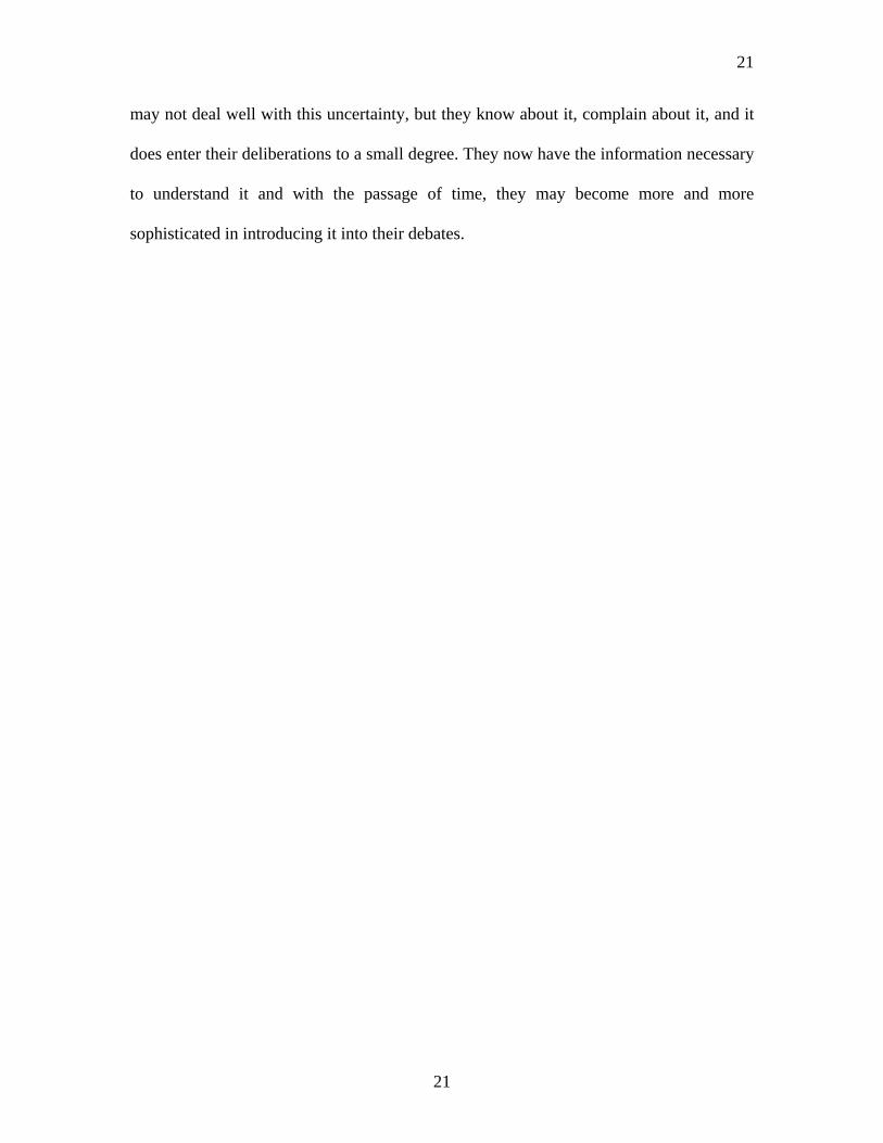
may not deal well with this uncertainty, but they know about it, complain about it, and it

does enter their deliberations to a small degree. They now have the information necessary

to understand it and with the passage of time, they may become more and more

sophisticated in introducing it into their debates.

21

22

Figure 1

Revisions as a Percent of GDP, Current Year Projections, 1984-2005

-1.5%

-1.0%

-0.5%

0.0%

0.5%

1.0%

1984 1987 1990 1993 1996 1999 2002 2005

Fiscal Year

% o

f GD

P

Source: Author's calculations

22

23

Figure 2

Revisions as a Percent of GDP, One-Year Projections, 1984-2005

-4.0%

-3.0%

-2.0%

-1.0%

0.0%

1.0%

2.0%

3.0%

1984 1987 1990 1993 1996 1999 2002 2005

Fiscal Year

% o

f GD

P

Source: Author's calculations

23

24

Figure 3

Revisions as a Percent of GDP, Five-Year Projections, 1989-2005

-4.0%

-3.0%

-2.0%

-1.0%

0.0%

1.0%

2.0%

3.0%

4.0%

1989 1990 1991 1992 1993 1994 1995 1996 1997 1998 1999 2000 2001 2002 2003 2004 2005

Fiscal Year

% o

f GD

P

Source: Author's calculations

24

25

References

Auerbach, Alan J. 1999. “On the Performance and Use of Government Revenue Forecasts.” National Tax Journal 52(4): 767–82

Bachman, Daniel. 1996. “What Economic Forecasters Really Do.” The WEFA Group,

Bala Cynwyd. Congressional Budget Office. 2006. “The Budget and Economic Outlook: Fiscal Years

2007 to 2016.” Washington, DC: U.S. Government Printing Office. ___. 2004. “Effective Federal Tax Rates Under Current Law, 2001 to 2014.”

Washington, DC: U.S. Government Printing Office. ___. 2006. “How CBO Forecasts Income.” Washington, DC: U.S. Government Printing

Office. Gramlich, Edward M. 1990. “U.S. Federal Budget Deficits and Gramm-Rudman-

Hollings.” American Economic Review 80(2): 75–80 Kitchen, John. 2003. “Observed Relationships between Economic and Technical Receipts

Revisions in Federal Budget Projections.” National Tax Journal 56(2): 337–53 Lucas, Robert E. 1976. “Econometric Policy Evaluation: A Critique.” In The Phillips

Curve and Labor Markets, edited by Karl Brunner and Alan Meltzer. Carnegie-Rochester Conference Series on Public Policy (1). Amsterdam: North Holland.

Wallis, W. Allen and Harry V. Roberts. 1956. Statistics: A New Approach. Glencoe, IL:

The Free Press.

25