feedback control of dynamic systems 8th edition franklin
TRANSCRIPT

2000
Solutions Manual: Chapter 28th Edition
Feedback Controlof Dynamic Systems
.
.
Gene F. Franklin.
J. David Powell.
Abbas Emami-Naeini.
.
.
.
Assisted by:H. K. AghajanH. Al-RahmaniP. CoulotP. DankoskiS. EverettR. FullerT. IwataV. JonesF. Safai
L. KobayashiH-T. Lee
E. ThuriyasenaM. Matsuoka
Copyright (c) 2019 Pearson Education
All rights reserved. No part of this publication may be reproduced, storedin a retrieval system, or transmitted, in any form or by any means, electronic,mechanical, photocopying, recording, or otherwise, without the prior permissionof the publisher.
Feedback Control of Dynamic Systems 8th Edition Franklin Solutions ManualFull Download: https://alibabadownload.com/product/feedback-control-of-dynamic-systems-8th-edition-franklin-solutions-manual/
This sample only, Download all chapters at: AlibabaDownload.com

Chapter 2
Dynamic Models
Problems and Solutions for Section 2.1
1. Write the di¤erential equations for the mechanical systems shown in Fig. 2.43.For (a) and (b), state whether you think the system will eventually decayso that it has no motion at all, given that there are non-zero initial condi-tions for both masses, and give a reason for your answer. Also, for part(c), answer the question for F=0.
2001

2002 CHAPTER 2. DYNAMIC MODELS
Fig. 2.43 Mechanical systems
Solution:
The key is to draw the Free Body Diagram (FBD) in order to keep thesigns right. For (a), to identify the direction of the spring forces on theobject, let x2 = 0 and �xed and increase x1 from 0. Then the k1 springwill be stretched producing its spring force to the left and the k2 springwill be compressed producing its spring force to the left also. You can usethe same technique on the damper forces and the other mass.
(a)
m1 m2
x1 x2
k (x x )2 1 2
k (x x )2 1 2
k (x3 2 y)k x1 1
b x1 1.
Free body diagram for Problem 2.1(a)
m1�x1 = �k1x1 � b1 _x1 � k2 (x1 � x2)m2�x2 = �k2 (x2 � x1)� k3 (x2 � y)
There is friction a¤ecting the motion of mass 1 which will continueto take energy out of the system as long as there is any movement ofx1:Mass 2 is undamped; therefore it will tend to continue oscillating.However, its motion will drive mass 1 through the spring; therefore,the entire system will continue to lose energy and will eventuallydecay to zero motion for both masses.

2003
m1 m2
x1 x2
x2k (x x )2 1 2
k (x x )2 1 2k x1 1
b x1 2.
x2
x2k3
Free body diagram for Problem 2.1(b)
m1�x1 = �k1x1 � k2(x1 � x2)m2�x2 = �k2(x2 � x1)� b1 _x2 � k3x2
Again, there is friction on mass 2 so there will continue to be a lossof energy as long as there is any motion; hence the motion of bothmasses will eventually decay to zero.
m1 m2
x1 x2
k (x x )2 1 2 k (x x )2 1 2
k x1 1
b (x x )1 1 2 b (x x )1 1 2. .. .
F
Free body diagram for Problem 2.1 (c)
m1�x1 = �k1x1 � k2(x1 � x2)� b1( _x1 � _x2)
m2�x2 = F � k2(x2 � x1)� b1( _x2 � _x1)
The situation here is similar to part (a). It is clear that the relativemotion between mass 1 and 2 would decay eventually, but as longas mass 1 is oscillating, it will drive some relative motion of the twomasses and that will cause energy loss in the damper. So the entiresystem will eventually decay to zero.
2. Write the di¤erential equations for the mechanical systems shown in Fig. 2.44.State whether you think the system will eventually decay so that it hasno motion at all, given that there are non-zero initial conditions for bothmasses, and give a reason for your answer.

2004 CHAPTER 2. DYNAMIC MODELS
Fig. 2.44 Mechanical system for Problem 2.2
Solution:
The key is to draw the Free Body Diagram (FBD) in order to keep thesigns right. To identify the direction of the spring forces on the left sideobject, let x2 = 0 and increase x1 from 0. Then the k1 spring on the leftwill be stretched producing its spring force to the left and the k2 springwill be compressed producing its spring force to the left also. You can usethe same technique on the damper forces and the other mass.
m1 m2
x1 x2
x2
k (x x )2 1 2
k x1 1 k1
b (x x )2 1 2 b (x x )2 1 2
. . . .
Free body diagram for Probelm 2.2
Then the forces are summed on each mass, resulting in
m1�x1 = �k1x1 � k2(x1 � x2)� b1( _x1 � _x2)
m2�x2 = k2(x1 � x2)� b1( _x1 � _x2)� k1x2
The relative motion between x1 and x2 will decay to zero due to thedamper. However, the two masses will continue oscillating togetherwithout decay since there is no friction opposing that motion and �exureof the end springs is all that is required to maintain the oscillation of thetwo masses. However, note that the two end springs have the same springconstant and the two masses are equal If this had not been true, the twomasses would oscillate with di¤erent frequencies and the damper wouldbe excited thus taking energy out of the system.
3. Write the equations of motion for the double-pendulum system shown inFig. 2.45. Assume the displacement angles of the pendulums are smallenough to ensure that the spring is always horizontal. The pendulum

2005
rods are taken to be massless, of length l, and the springs are attached3/4 of the way down.
Fig. 2.45 Double pendulum
Solution:
1θ 2θ
k
1sin43
θl 2sin43
θl
m m
l43
De�ne coordinates
If we write the moment equilibrium about the pivot point of the left pen-dulem from the free body diagram,
M = �mgl sin �1 � k3
4l (sin �1 � sin �2) cos �1
3
4l = ml2��1
2006 CHAPTER 2. DYNAMIC MODELS
ml2��1 +mgl sin �1 +9
16kl2 cos �1 (sin �1 � sin �2) = 0
Similary we can write the equation of motion for the right pendulem
�mgl sin �2 + k3
4l (sin �1 � sin �2) cos �2
3
4l = ml2��2
As we assumed the angles are small, we can approximate using sin �1 ��1; sin �2 � �2, cos �1 � 1, and cos �2 � 1. Finally the linearized equationsof motion becomes,
ml��1 +mg�1 +9
16kl (�1 � �2) = 0
ml��2 +mg�2 +9
16kl (�2 � �1) = 0
Or
��1 +g
l�1 +
9
16
k
m(�1 � �2) = 0
��2 +g
l�2 +
9
16
k
m(�2 � �1) = 0
4. Write the equations of motion of a pendulum consisting of a thin, 2-kgstick of length l suspended from a pivot. How long should the rod be inorder for the period to be exactly 1 sec? (The inertia I of a thin stickabout an endpoint is 1
3ml2. Assume � is small enough that sin � �= �.)
Solution:
Let�s use Eq. (2.14)
M = I�;

2007
mg
θ
2lO
De�ne coordinatesand forces
Moment about point O.
MO = �mg � l
2sin � = IO��
=1
3ml2��
�� +3g
2lsin � = 0
As we assumed � is small,
�� +3g
2l� = 0
The frequency only depends on the length of the rod
!2 =3g
2l
T =2�
!= 2�
s2l
3g= 2
l =3g
8�2= 0:3725m

2008 CHAPTER 2. DYNAMIC MODELS
Grandfather clocks have a period of 2 sec, i.e., 1 sec for a swing from oneside to the other. This pendulum is shorter because the period is faster.But if the period had been 2 sec, the pendulum length would have been1.5 meters, and the clock itself would have been about 2 meters to housethe pendulum and the clock face.
<Side notes>
(a) Compare the formula for the period, T = 2�q
2l3g with the well known
formula for the period of a point mass hanging with a string with
length l. T = 2�q
lg .
(b) Important!
In general, Eq. (2.14) is valid only when the reference point forthe moment and the moment of inertia is the mass center of thebody. However, we also can use the formular with a reference pointother than mass center when the point of reference is �xed or notaccelerating, as was the case here for point O.
5. For the car suspension discussed in Example 2.2, plot the position of thecar and the wheel after the car hits a �unit bump�(i.e., r is a unit step)using Matlab. Assume thatm1 = 10 kg,m2 = 350 kg, kw = 500; 000 N=m,ks = 10; 000 N=m. Find the value of b that you would prefer if you werea passenger in the car.
Solution:
The transfer function of the suspension was given in the example in Eq.(2.12) to be:
(a)
Y (s)
R(s)=
kwbm1m2
(s+ ksb )
s4 + ( bm1+ b
m2)s3 + ( ksm1
+ ksm2+ kw
m1)s2 + ( kwb
m1m2)s+ kwks
m1m2
:
This transfer function can be put directly into Matlab along with thenumerical values as shown below. Note that b is not the damping ra-tio, but damping. We need to �nd the proper order of magnitude forb, which can be done by trial and error. What passengers feel is theposition of the car. Some general requirements for the smooth ridewill be, slow response with small overshoot and oscillation. Whilethe smallest overshoot is with b=5000, the jump in car position hap-pens the fastest with this damping value.

2009
From the �gures, b � 3000 appears to be the best compromise. Thereis too much overshoot for lower values, and the system gets too fast(and harsh) for larger values.

2010 CHAPTER 2. DYNAMIC MODELS
% Problem 2.5 Using state space methods% Can also be done using the transfer function aboveclear all, close all
m1 = 10;m2 = 350;kw = 500000;ks = 10000;Bd = [ 1000 3000 4000 5000];t = 0:0.01:2;
for i = 1:4b = Bd(i);A=[0 1 0 0;-( ks/m1 + kw/m1 ) -b/m1 ks/m1 b/m1;
0 0 0 1; ks/m2 b/m2 -ks/m2 -b/m2 ];B=[0; kw/m1; 0; 0 ];C=[ 1 0 0 0; 0 0 1 0 ];D=0;y=step(A,B,C,D,1,t);subplot(2,2,i);plot( t, y(:,1), �:�, t, y(:,2), �-�);legend(�Wheel�,�Car�);ttl = sprintf(�Response with b = %4.1f �,b );title(ttl);
end
6. For the quadcopter shown in Figs. 2.13 and 2.14:
(a) Determine the appropriate commands to rotor #s 1, 2, 3, & 4 so apure vertical force will be applied to the quadcopter, that is, a force thatwill have no e¤ect on pitch, roll, or yaw.
(b) Determine the transfer function between Fh, and altitude, h. That is,�nd h(s)=Fh(s).
Solution:
(a) To increase the lifting force, we want to increase the speed of all fourrotors. Since two rotors are rotating CW and two are rotating CCW,there will be no net torque about the yaw axis. Since rotor #s 1 and 3are rotating CW, we want to apply a positive torque to those two rotors,i.e., F
�T1 = �T3 = +KFh;
where Fh is the command for an increased lift for motion in the upwardvertical direction and K is the scale factor between torque and lift. Like-wise, since rotor #s 2 and 4 are rotating in the CCW direction, we wanttp apply a negative torque to those two rotors, i.e.,

2011
�T2 = �T4 = �KFh;
(b) Assuming the mass of the quadrotor is m, the transfer function wouldbe
h(s)
Fh(s)=
1
ms2
7. Automobile manufacturers are contemplating building active suspensionsystems. The simplest change is to make shock absorbers with a change-able damping, b(u1): It is also possible to make a device to be placed inparallel with the springs that has the ability to supply an equal force, u2;in opposite directions on the wheel axle and the car body.
(a) Modify the equations of motion in Example 2.2 to include such con-trol inputs.
(b) Is the resulting system linear?
(c) Is it possible to use the forcer, u2; to completely replace the springsand shock absorber? Is this a good idea?
Solution:
(a) The FBD shows the addition of the variable force, u2; and shows bas in the FBD of Fig. 2.5, however, here b is a function of the controlvariable, u1: The forces below are drawn in the direction that wouldresult from a positive displacement of x.
m1 m2
k (xy)s
k (xy)sk (xr)w
b(xy)
b(xy)
.
.
x
u2
u2
y
.
.
Free body diagram
m1�x = b (u1) ( _y � _x) + ks (y � x)� kw (x� r)� u2m2�y = �ks (y � x)� b (u1) ( _y � _x) + u2

2012 CHAPTER 2. DYNAMIC MODELS
(b) The system is linear with respect to u2 because it is additive. Butb is not constant so the system is non-linear with respect to u1 be-cause the control essentially multiplies a state element. So if we addcontrollable damping, the system becomes non-linear.
(c) It is technically possible. However, it would take very high forcesand thus a lot of power and is therefore not done. It is a much bet-ter solution to modulate the damping coe¢ cient by changing ori�cesizes in the shock absorber and/or by changing the spring forces byincreasing or decreasing the pressure in air springs. These featuresare now available on some cars... where the driver chooses betweena soft or sti¤ ride.
8. In many mechanical positioning systems there is �exibility between onepart of the system and another. An example is shown in Figure 2.7where there is �exibility of the solar panels. Figure 2.46 depicts such asituation, where a force u is applied to the mass M and another massm is connected to it. The coupling between the objects is often modeledby a spring constant k with a damping coe¢ cient b, although the actualsituation is usually much more complicated than this.
(a) Write the equations of motion governing this system.
(b) Find the transfer function between the control input, u; and theoutput, y:
Fig. 2.46 Schematic of a system with�exibility
Solution:
(a) The FBD for the system is

2013
m
x y
k(x y)k(x y)
b(x y) b(x y). .. .
M u
Free body diagrams
which results in the equations
m�x = �k (x� y)� b ( _x� _y)
M �y = u+ k (x� y) + b ( _x� _y)
or
�x+k
mx+
b
m_x� k
my � b
m_y = 0
� k
Mx� b
M_x+ �y +
k
My +
b
M_y =
1
Mu
(b) If we make Laplace Transform of the equations of motion
s2X +k
mX +
b
msX � k
mY � b
msY = 0
� k
MX � b
MsX + s2Y +
k
MY +
b
MsY =
1
MU
In matrix form,�ms2 + bs+ k � (bs+ k)� (bs+ k) Ms2 + bs+ k
� �XY
�=
�0U
�From Cramer�s Rule,
Y =
det
�ms2 + bs+ k 0� (bs+ k) U
�det
�ms2 + bs+ k � (bs+ k)� (bs+ k) Ms2 + bs+ k
�=
ms2 + bs+ k
(ms2 + bs+ k) (Ms2 + bs+ k)� (bs+ k)2U
Finally,

2014 CHAPTER 2. DYNAMIC MODELS
Y
U=
ms2 + bs+ k
(ms2 + bs+ k) (Ms2 + bs+ k)� (bs+ k)2
=ms2 + bs+ k
mMs4 + (m+M)bs3 + (M +m)ks2
9. Modify the equation of motion for the cruise control in Example 2.1,Eq(2.4), so that it has a control law; that is, let
u = K(vr � v);
where
vr = reference speed
K = constant:
This is a �proportional�control law where the di¤erence between vr andthe actual speed is used as a signal to speed the engine up or slow it down.Put the equations in the standard state-variable form with vr as the inputand v as the state. Assume that m = 1500 kg and b = 70 N � s=m; and�nd the response for a unit step in vr using Matlab. Using trial and error,�nd a value of K that you think would result in a control system in whichthe actual speed converges as quickly as possible to the reference speedwith no objectional behavior.
Solution:
_v +b
mv =
1
mu
substitute in u = K (vr � v)
_v +b
mv =
1
mu =
K
m(vr � v)
Rearranging, yields the closed-loop system equations,
_v +b
mv +
K
mv =
K
mvr
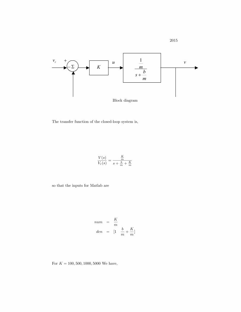
A block diagram of the scheme is shown below where the car dynamicsare depicted by its transfer function from Eq. 2.7.
2015
Block diagram
The transfer function of the closed-loop system is,
V (s)
Vr(s)=
Km
s+ bm +
Km
so that the inputs for Matlab are
num =K
m
den = [1b
m+K
m]
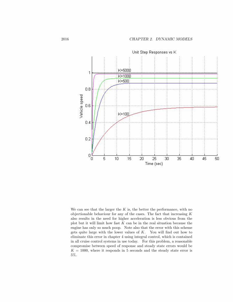
For K = 100; 500; 1000; 5000 We have,
2016 CHAPTER 2. DYNAMIC MODELS
We can see that the larger the K is, the better the performance, with noobjectionable behaviour for any of the cases. The fact that increasing Kalso results in the need for higher acceleration is less obvious from theplot but it will limit how fast K can be in the real situation because theengine has only so much poop. Note also that the error with this schemegets quite large with the lower values of K. You will �nd out how toeliminate this error in chapter 4 using integral control, which is containedin all cruise control systems in use today. For this problem, a reasonablecompromise between speed of response and steady state errors would beK = 1000; where it responds in 5 seconds and the steady state error is5%.

2017
% Problem 2.9clear all, close all
% datam = 1500;b = 70;k = [ 100 500 1000 5000 ];
% Overlay the step responsehold ont=0:0.2:50;for i=1:length(k)K=k(i);num =K/m;den = [1 b/m+K/m];sys=tf(num,den);y = step(sys,t);plot(t,y)
endhold o¤

2018 CHAPTER 2. DYNAMIC MODELS
10. Determine the dynamic equations for lateral motion of the robot in Fig.2.47. Assume it has 3 wheels with the front a single, steerable wheelwhere you have direct control of the rate of change of the steering angle,Usteer, with geometry as shown in Fig. 2.48. Assume the robot is go-ing in approximately a straight line and its angular deviation from thatstraight line is very small Also assume that the robot is traveling at aconstant speed, Vo. The dynamic equations relating the lateral veloc-ity of the center of the robot as a result of commands in Usteer is desired.
.Fig. 2.47 Robot for delivery of hospital supplies Source: AP Images
Fig. 2.48 Model for robot motion

2019
Solution:
This is primarily a problem in kinematics. First, we know that the controlinput, Usteer; is the time rate of change of the steering wheel angle, so
_�s = Usteer
When �s is nonzero, the cart will be turning, so that its orientation wrtthe x axis will change at the rate
_ =Vo�sL:
as shown by the diagram below.
Diagram showing turning rate due to �sT
The actual change in the carts lateral position will then be proportionalto according to
_y = Vo
as shown below.

2020 CHAPTER 2. DYNAMIC MODELS
Lateral motion as a function of
These linear equations will hold providing and �s stay small enoughthat sin ' ; and sin �s ' �s:Combining them all, we obtain,
...y =
V 2oLUsteer
Note that no dynamics come into play here. It was assumed that thevelocity is constant and the front wheel angle time rate of change is directlycommanded. Therefore, there was no need to invoke Eqs (2.1) or (2.10).As you will see in future chapters, feedback control of such a system witha triple integration is tricky and needs signi�cant damping in the feedbackpath to achieve stability.
11. Determine the pitch, yaw, and roll control equations for the hexacoptershown in Fig. 2.49 that are similar to those for the quadcopter given inEqs. (2.18) to (2.20).
Fig. 2.49 Hexacopter

2021
Assume that rotor #1 is in the direction of �ight and the remaining rotorsare numbered CW from that rotor. In other words, rotors #1 and #4will determine the pitch motion. Rotor #s 2, 3, 5, & 6 will determineroll motion. Pitch, roll and yaw motions are de�ned by the coordinatesystem shown in Fig. 2.14 in Example 2.5. In addition to developing theequations for the 3 degrees of freedom in terms of how the six rotor motorsshould be commanded (similar to thoseforthe quadrotorinEqs. (2.18)�(2.20)), it will also be necessary to decide which rotors are turning CWand which ones are turning CCW. The direction of rotation for the rotorsneeds to be selected so there is no net torque about the vertical axis; thatis, the hexicopter will have no tendancy for yaw rotation in steadystate.Furthermore, a control action to a¤ect pitch should have no e¤ect on yawor roll. Likewise, a control action for roll should have no e¤ect on pitchor yaw, and a control action for yaw should have no e¤ect on pitch orroll. In other words, the control actions should produce no cross-couplingbetween pitch, roll, and yaw just as was the case for the quadcopter inExample 2.5.
Solution: For starters, the instructions above give us the following def-initions
Hexacopter coordinate system de�nition
To obtain some symmetry in the rotations, let�s assign rotor #s 1, 3, & 5to rotate CW, while rotor #s 2, 4, & 6 rotate CCW.
Now let�s start out by examining the yaw torque e¤ects. If we assumethe same control action as we found for the quadrotor in Eq. (2.20), wewould apply a negative torque on all six rotors. This will clearly producea positive yawing torque on the hexacopter with no net change in vertical

2022 CHAPTER 2. DYNAMIC MODELS
lift for the same reasons given on pages 38 and 39. However, it notnecessarily produce zero torque about the pitch and roll axes. So let�scheck that and adjust things if required. Unlike the quadrotor wherethe two rotors on the x-axis were both turning CW, rotors1 and 4 areturning in the opposite direction. So in this case, giving those two rotorsan equal negative torque will speed one up rotor 4 and slow down,rotor 1,thus producing a negative torque about the y-axis. However, note thatrotors 2 and 6 will speed up, while rotors 3 and 5 will slow down, thusproducing a positive torque.about the y-axis. These two torques canceleach other because the angle between rotors 2, 3, 5 & 6 and the y-axis areall 30o between the arms and the y-axis. Since the sine of 30o = 1/2, thatmeans that the torque about the y-axis from rotors 2, 3, 5 & 6 will o¤setthe torque from rotors 1 & 4. For no roll moment, we require a net zerotorque about the x-axis. Rotors 1 & 4 are on the x-axis, so no torquefrom them. Rotors 2 & 6 are both CCW, so they produce no net torqueabout the x-axis, and the same applies for rotors 3 & 5; hence when weapply an equal torque on all six rotors in the same direction along thez-axis, we obtain a yaw torque with no e¤ect on pitch or roll or a verticalforce. So, the control using:
Yaw control: �T1 = �T2 = �T3 = �T4 = �T5 = �T6 = �T ;
will produce motion in yaw, with no e¤ect on pitch, roll, or verticalmotion.
For pitch control, we want an increase in the speed and lift of theCW rotor 1 (ie a positive �T1) and a decrease in the speed of the CCWrotor 4, which requires a positive �T4; so �T1 = �T4 = +T�. But notethat this action will produce a yawing torque, which.can be canceled if weapply an equal and opposite yawing torque from rotors 2, 3, 5, 6. Thisaccomplished by �T2 = �T3 = �T5 = �T6 = �T�=2: In fact, this additionalcontrol will also add to the torque about the pitch (y-axis) by 50% whilehaving no e¤ect on roll. Thus the control using:
Pitch control: �T1 = 2 ��T2 = 2 ��T3 = ��T4 = 2 ��T5 = 2 ��T6 = �2
3T�;
will produce motion in pitch, with no e¤ect on yaw, roll, or vertical mo-tion.
For roll control, by increasing the speed of rotors 5 & 6, and decreasingthe speed of rotors 2 & 3, we will obtain a positive roll torque about thex-axis. No change is needed for rotors 1 & 4. To accomplish thesespeed changes, we need to apply a positive torque to the CW rotor 5 anda negative torque to the CCW rotor 6. Likewise, we need a positivetorque to the CCW rotor 2 and a negative torque to the CW rotor 3.

2023
Since the torques applied are half positive and half negative, there will beno yaw torque. Furthermore, there will be no pitch torque of change inoverall lift with these torque applications. However, the moment arm isnot 1 arm length; rather it is cos(30o), so to keep the scale factor for thetwo arms consistent with the pitch axis, we need to divide by 2 � cos(30o):Therefore, the control using:
Roll control: �T2 = ��T3 = �T5 = ��T6 = T�=(2 � cos(30o));
will produce motion in roll, with no e¤ect on pitch, yaw, or vertical mo-tion.
12. In most cases, quadcopters have a camera mounted that does not swivelin the x� y plane and its direction of view is oriented at 45o to the armssupporting the rotors. Therefore, these drones typically �y in a directionthat is aligned with the camera rather than along an axis containing twoof the rotors. To simplify the �ight dynamics, the x-direction of thecoordinate system is aligned with the camera direction. Based on thecoordinate de�nitions for the axes in Fig. 2.14, assume the x-axis lies halfway between rotors # 1 and 2 and determine the rotor commands for thefour rotors that would accomplish independent motion for pitch, roll, andyaw.
Solution:
The orientation of the coordinate system and arrangement of the rotors is

2024 CHAPTER 2. DYNAMIC MODELS
Coorinate system and rotor arrangement
It should be clear from the discussion on pages 38 and 39 of the book (plusthe discussion here for Problem 2.11) that the following commands to therotors produces the desired independent motion:
Roll control: �T1 = �T2 = ��T3 = ��T4 = T�;Pitch control: �T1 = ��T2 = ��T3 = �T4 = T�;Yaw control: �T1 = �T2 = �T3 = �T4 = T :
Problems and Solutions for Section 2.2
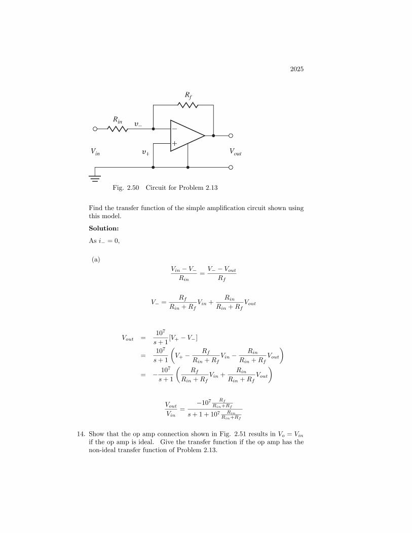
13. A �rst step toward a realistic model of an op amp is given by the equationsbelow and shown in Fig. 2.50.
Vout =107
s+ 1[V+ � V�]
i+ = i� = 0
2025
Fig. 2.50 Circuit for Problem 2.13
Find the transfer function of the simple ampli�cation circuit shown usingthis model.
Solution:
As i� = 0,
(a)Vin � V�Rin
=V� � Vout
Rf
V� =Rf
Rin +RfVin +
RinRin +Rf
Vout
Vout =107
s+ 1[V+ � V�]
=107
s+ 1
�V+ �
RfRin +Rf
Vin �Rin
Rin +RfVout
�= � 107
s+ 1
�Rf
Rin +RfVin +
RinRin +Rf
Vout
�
VoutVin
=�107 Rf
Rin+Rf
s+ 1 + 107 Rin
Rin+Rf
14. Show that the op amp connection shown in Fig. 2.51 results in Vo = Vinif the op amp is ideal. Give the transfer function if the op amp has thenon-ideal transfer function of Problem 2.13.
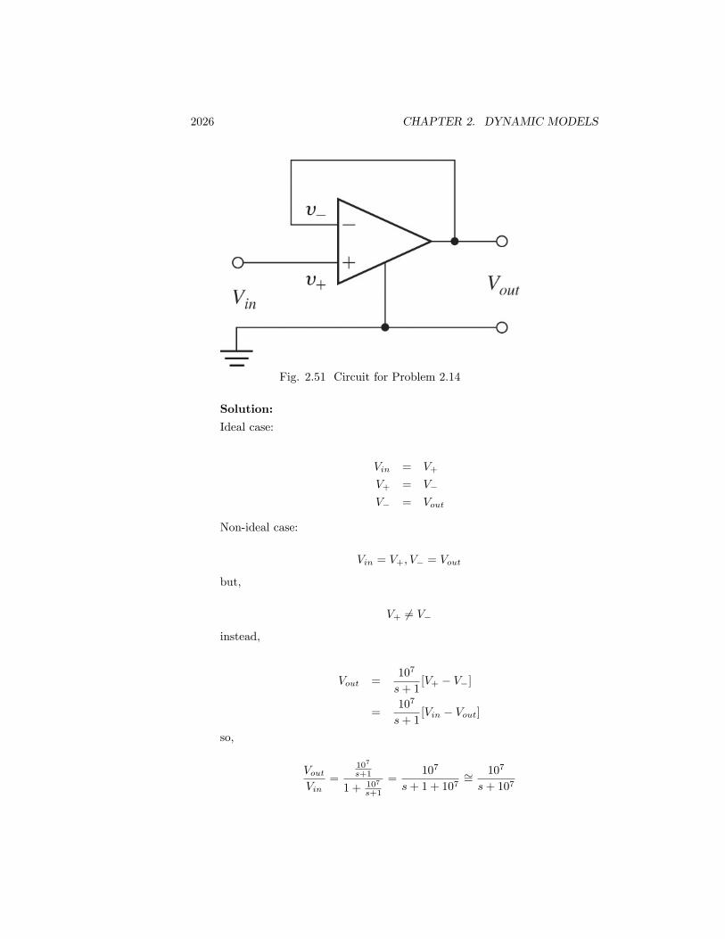
2026 CHAPTER 2. DYNAMIC MODELS
Fig. 2.51 Circuit for Problem 2.14
Solution:
Ideal case:
Vin = V+
V+ = V�
V� = Vout
Non-ideal case:
Vin = V+; V� = Vout
but,
V+ 6= V�instead,
Vout =107
s+ 1[V+ � V�]
=107
s+ 1[Vin � Vout]
so,
VoutVin
=107
s+1
1 + 107
s+1
=107
s+ 1 + 107�=
107
s+ 107

2027
15. A common connection for a motor power ampli�er is shown in Fig. 2.52.The idea is to have the motor current follow the input voltage and theconnection is called a current ampli�er. Assume that the sense resistor,Rs is very small compared with the feedback resistor, R and �nd thetransfer function from Vin to Ia: Also show the transfer function whenRf =1:
Node A
Node B
Fig. 2.52 Op Amp circuit for Problem 2.15 with nodesmarked.
Solution:
At node A,Vin � 0Rin
+Vout � 0Rf
+VB � 0R
= 0 (201)
At node B, with Rs � R
Ia +0� VBR
+0� VBRs
= 0 (202)
VB =RRsR+Rs
Ia
VB � RsIa
The dynamics of the motor is modeled with negligible inductance as
Jm��m + b _�m = KtIa (203)
Jms+ b = KtIa

2028 CHAPTER 2. DYNAMIC MODELS
At the output, from Eq. (202). Eq. (203) and the motor equation Va =IaRa +Kes
Vo = IaRs + Va
= IaRs + IaRa +KeKtIaJms+ b
Substituting this into Eq.(201)
VinRin
+1
Rf
�IaRs + IaRa +Ke
KtIaJms+ b
�+IaRsR
= 0
This expression shows that, in the steady state when s ! 0; the currentis proportional to the input voltage.
If fact, the current ampli�er normally has no feedback from the outputvoltage, in which case Rf !1 and we have simply
IaVin
= � R
RinRs
16. An op amp connection with feedback to both the negative and the positiveterminals is shown in Fig 2.53. If the op amp has the non-ideal transferfunction given in Problem 13, give the maximum value possible for thepositive feedback ratio, P =
r
r +Rin terms of the negative feedback
ratio,N =Rin
Rin +Rffor the circuit to remain stable.
Fig. 2.53 Op Amp circuit for Problem 2.16

2029
Solution:
Vin � V�Rin
+Vout � V�
Rf= 0
Vout � V+R
+0� V+r
= 0
V� =Rf
Rin +RfVin +
RinRin +Rf
Vout
= (1�N)Vin +NVoutV+ =
r
r +RVout = PVout
Vout =107
s+ 1[V+ � V�]
=107
s+ 1[PVout � (1�N)Vin �NVout]
VoutVin
=
107
s+ 1(1�N)
107
s+ 1P � 107
s+ 1N � 1
=107 (1�N)
107P � 107N � (s+ 1)
=�107 (1�N)
s+ 1� 107P + 107N
0 < 1� 107P + 107NP < N + 10�7
17. Write the dynamic equations and �nd the transfer functions for the circuitsshown in Fig. 2.54.
(a) passive lead circuit
(b) active lead circuit
(c) active lag circuit.

2030 CHAPTER 2. DYNAMIC MODELS
(d) passive notch circuit
Fig. 2.54 (a) Passive lead, (b) active lead, (c)active lag, (d) passive notch circuits

2031
Solution:
(a) Passive lead circuit
With the node at y+, summing currents into that node, we get
Vu � VyR1
+ Cd
dt(Vu � Vy)�
VyR2
= 0 (204)
rearranging a bit,
C _Vy +
�1
R1+1
R2
�Vy = C _Vu +
1
R1Vu
and, taking the Laplace Transform, we get
Vy(s)
Vu(s)=
Cs+ 1R1
Cs+�1R1+ 1
R2
�(b) Active lead circuit
inV outV
C
V
1R 2R
fR
Active lead circuit with node marked
Vin � VR2
+0� VR1
+ Cd
dt(0� V ) = 0 (205)
Vin � VR2
=0� VoutRf
(206)
We need to eliminate V . From Eq. (206),
V = Vin +R2RfVout
Substitute V �s in Eq. (205).

2032 CHAPTER 2. DYNAMIC MODELS
1
R2
�Vin � Vin �
R2RfVout
�� 1
R1
�Vin +
R2RfVout
��C
�_Vin +
R2Rf
_Vout
�= 0
1
R1Vin + C _Vin = �
1
Rf
��1 +
R2R1
�Vout +R2C _Vout
�Laplace Transform
VoutVin
=Cs+ 1
R1
� 1Rf
�R2Cs+ 1 +
R2
R1
�= �Rf
R2
s+ 1R1C
s+ 1R1C
+ 1R2C
We can see that the pole is at the left side of the zero, which meansa lead compensator.
(c) active lag circuit
inR
inV outV
1R2R
C
V
Active lag circuit with node marked
Vin � 0Rin
=0� VR2
=V � VoutR1
+ Cd
dt(V � Vout)
V = � R2Rin
Vin
VinRin
=� R2
RinVin � VoutR1
+ Cd
dt
�� R2Rin
Vin � Vout�
=1
R1
�� R2Rin
Vin � Vout�+ C
�� R2Rin
_Vin � _Vout
�

2033
1
Rin
�1 +
R2R1
�Vin +
1
RinR2C _Vin = �
1
R1Vout � C _Vout
VoutVin
= � R1Rin
R2Cs+ 1 +R2
R1
R1Cs+ 1
= � R2Rin
s+ 1R2C
+ 1R1C
s+ 1R1C
We can see that the pole is at the right side of the zero, which meansa lag compensator.
(d) notch circuit
outV
C1VC
C2
R R2/R
+ +
− −
inV
2V
Passive notch �lter with nodes marked
Cd
dt(Vin � V1) +
0� V1R=2
+ Cd
dt(Vout � V1) = 0
Vin � V2R
+ 2Cd
dt(0� V2) +
Vout � V2R
= 0
Cd
dt(V1 � Vout) +
V2 � VoutR
= 0
We need to eliminat V1; V2 from three equations and �nd the relationbetween Vin and Vout
V1 =Cs
2�Cs+ 1
R
� (Vin + Vout)V2 =
1R
2�Cs+ 1
R
� (Vin + Vout)

2034 CHAPTER 2. DYNAMIC MODELS
CsV1 � CsVout +1
RV2 �
1
RVout
= CsCs
2�Cs+ 1
R
� (Vin + Vout) + 1
R
1R
2�Cs+ 1
R
� (Vin + Vout)� �Cs+ 1
R
�Vout
= 0
C2s2 + 1R2
2�Cs+ 1
R
�Vin =
"�Cs+
1
R
��C2s2 + 1
R2
2�Cs+ 1
R
�#VoutVoutVin
=
C2s2+ 1R2
2(Cs+ 1R )�
Cs+ 1R
�� C2s2+ 1
R2
2(Cs+ 1R )
=
�C2s2 + 1
R2
�2�Cs+ 1
R
�2 � �C2s2 + 1R2
�=
C2�s2 + 1
R2C2
�C2s2 + 4CsR + 1
R2
=s2 + 1
R2C2
s2 + 4RC s+
1R2C2
18. The very �exible circuit shown in Fig. 2.55 is called a biquad becauseits transfer function can be made to be the ratio of two second-order orquadratic polynomials. By selecting di¤erent values for Ra; Rb; Rc; andRd the circuit can realise a low-pass, band-pass, high-pass, or band-reject(notch) �lter.
(a) Show that if Ra = R; and Rb = Rc = Rd =1; the transfer functionfrom Vin to Vout can be written as the low-pass �lter
VoutVin
=A
s2
!2n+ 2�
s
!n+ 1
where
A =R
R1
!n =1
RC
� =R
2R2

2035
(b) Using the MATLAB comand step compute and plot on the samegraph the step responses for the biquad of Fig. 2.55 for A = 2;!n = 2; and � = 0:1; 0:5; and 1:0:
Fig. 2.55 Op-amp biquad
Solution:
Before going in to the speci�c problem, let�s �nd the general form of thetransfer function for the circuit.
VinR1
+V3R
= ��V1R2
+ C _V1
�V1R
= �C _V2V3 = �V2
V3Ra
+V2Rb
+V1Rc
+VinRd
= �VoutR
There are a couple of methods to �nd the transfer function from Vin toVout with set of equations but for this problem, we will directly solve forthe values we want along with the Laplace Transform.
From the �rst three equations, slove for V1;V2.
VinR1
+V3R
= ��1
R2+ Cs
�V1
V1R
= �CsV2V3 = �V2

2036 CHAPTER 2. DYNAMIC MODELS
�1
R2+ Cs
�V1 �
1
RV2 = � 1
R1Vin
1
RV1 + CsV2 = 0
�1R2+ Cs � 1
R1R Cs
� �V1V2
�=
�� 1R1Vin0
�
�V1V2
�=
1�1R2+ Cs
�Cs+ 1
R2
�Cs 1
R� 1R
1R2+ Cs
� �� 1R1Vin0
�
=1
C2s2 + CR2s+ 1
R2
�� CR1sVin
1RR1
Vin
�
Plug in V1, V2 and V3 to the fourth equation.
V3Ra
+V2Rb
+V1Rc
+VinRd
=
�� 1
Ra+1
Rb
�V2 +
1
RcV1 +
1
RdVin
=
�� 1
Ra+1
Rb
� 1RR1
C2s2 + CR2s+ 1
R2
Vin +1
Rc
� CR1s
C2s2 + CR2s+ 1
R2
Vin +1
RdVin
=
"�� 1
Ra+1
Rb
� 1RR1
C2s2 + CR2s+ 1
R2
+1
Rc
� CR1s
C2s2 + CR2s+ 1
R2
+1
Rd
#Vin
= �VoutR
Finally,
VoutVin
= �R"�� 1
Ra+1
Rb
� 1RR1
C2s2 + CR2s+ 1
R2
+1
Rc
� CR1s
C2s2 + CR2s+ 1
R2
+1
Rd
#
= �R
�� 1Ra+ 1
Rb
�1
RR1� 1
Rc
CR1s+ 1
Rd
�C2s2 + C
R2s+ 1
R2
�C2s2 + C
R2s+ 1
R2
= � R
C2
C2
Rds2 +
�1Rd
CR2� 1
Rc
CR1
�s+
�1Rb� 1
Ra
�1
RR1+ 1
Rd
1R2
s2 + 1R2C
s+ 1(RC)2

2037
(a) If Ra = R; and Rb = Rc = Rd =1;
VoutVin
= � R
C2
C2
Rds2 +
�1Rd
CR2� 1
Rc
CR1
�s+
�1Rb� 1
Ra
�1
RR1+ 1
Rd
1R2
s2 + 1R2C
s+ 1(RC)2
= � R
C2� 1R
1RR1
s2 + 1R2C
s+ 1(RC)2
=1
RR1C2
s2 + 1R2C
s+ 1(RC)2
=RR1
(RC)2s2 + R2C
R2s+ 1
So,
R
R1= A
(RC)2=
1
!2n
2�
!n=
R2C
R2
!n =1
RC
� =!n2
R2C
R2=
1
2RC
R2C
R2=
R
2R2
(b) Step response using MatLab

2038 CHAPTER 2. DYNAMIC MODELS
Step responses
% Problem 2.18A = 2;wn = 2;z = [ 0.1 0.5 1.0 ];
hold onfor i = 1:3
num = [ A ];den = [ 1/wn^2 2*z(i)/wn 1 ]step( num, den )
endhold o¤
19. Find the equations and transfer function for the biquad circuit of Fig. 2.55if Ra = R; Rd = R1 and Rb = Rc =1:
Solution:
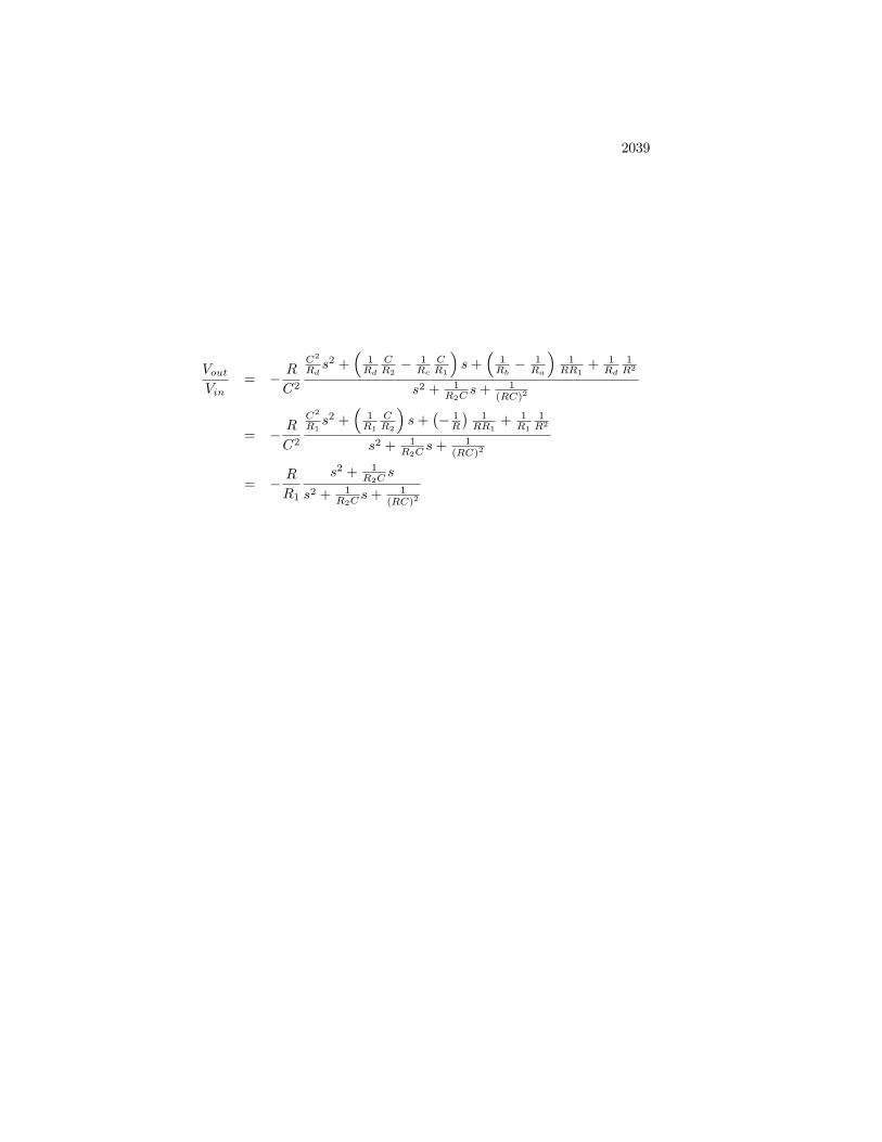
2039
VoutVin
= � R
C2
C2
Rds2 +
�1Rd
CR2� 1
Rc
CR1
�s+
�1Rb� 1
Ra
�1
RR1+ 1
Rd
1R2
s2 + 1R2C
s+ 1(RC)2
= � R
C2
C2
R1s2 +
�1R1
CR2
�s+
�� 1R
�1
RR1+ 1
R1
1R2
s2 + 1R2C
s+ 1(RC)2
= � RR1
s2 + 1R2C
s
s2 + 1R2C
s+ 1(RC)2
2040 CHAPTER 2. DYNAMIC MODELS
Problems and Solutions for Section 2.3
20. The torque constant of a motor is the ratio of torque to current and isoften given in ounce-inches per ampere. (ounce-inches have dimensionforce-distance where an ounce is 1=16 of a pound.) The electric constantof a motor is the ratio of back emf to speed and is often given in volts per1000 rpm. In consistent units the two constants are the same for a givenmotor.
(a) Show that the units ounce-inches per ampere are proportional tovolts per 1000 rpm by reducing both to MKS (SI) units.
(b) A certain motor has a back emf of 30 V at 1000 rpm. What is itstorque constant in ounce-inches per ampere?
(c) What is the torque constant of the motor of part (b) in newton-metersper ampere?
Solution:
Before going into the problem, let�s review the units.
� Some remarks on non SI units.�Ounce
1oz = 2:835� 10�2 kg
Actuall, the ounce is a unit of mass, but like pounds, it is com-monly used as a unit of force. If we translate it as force,
1oz(f) = 2:835� 10�2 kgf = 2:835� 10�2 � 9:81N = 0:2778N
� Inch
1 in = 2:540� 10�2m
�RPM (Revolution per Minute)
1 RPM =2� rad
60 s=�
30rad/ s
� Relation between SI units�Voltage and Current
V olts � Current(amps) = Power = Energy(joules)= sec
V olts =Joules= sec
amps=Newton�meters= sec
amps

2041
(a) Relation between torque constant and electric constant.Torque constant:
1 ounce� 1 inch1 Ampere
=0:2778N� 2:540� 10�2m
1A= 7:056�10�3Nm=A
Electric constant:
1V
1000 RPM=
1J=(A sec)1000� �
30 rad/ s= 9:549� 10�3Nm=A
So,
1 oz in=A =7:056� 10�39:549� 10�3 V=1000 RPM
= (0:739) V=1000 RPM
and the constant of proportionality = (0:739) :
(b)
30V=1000 RPM = 30� 1
0:739oz in=A = 40:6 oz in=A
(c)
30V=1000 RPM = 30� 9:549� 10�3Nm=A = 0:286Nm=A
21. The electromechanical system shown in Fig. 2.56 represents a simpli�edmodel of a capacitor microphone. The system consists in part of a parallelplate capacitor connected into an electric circuit. Capacitor plate a isrigidly fastened to the microphone frame. Sound waves pass through themouthpiece and exert a force fe(t) on plate b, which has mass M and isconnected to the frame by a set of springs and dampers. The capacitanceC is a function of the distance x between the plates, as follows:
C(x) ="A
x;
where
" = dielectric constant of the material between the plates;
A = surface area of the plates:
The charge q and the voltage e across the plates are related by
q = C(x)e:
The electric �eld in turn produces the following force fe on the movableplate that opposes its motion:
fe =q2
2"A

2042 CHAPTER 2. DYNAMIC MODELS
(a) Write di¤erential equations that describe the operation of this sys-tem. (It is acceptable to leave in nonlinear form.)
(b) Can one get a linear model?
(c) What is the output of the system?
Fig. 2.56 Simpli�ed model for capacitor microphone
Solution:
(a) The free body diagram of the capacitor plate b
x
M( )tf
Kx−xB&−
( ) efx&sgn−
e
Free body diagram for Prob. 2.21
So the equation of motion for the plate is
M �x+B _x+Kx+ fesgn ( _x) = fs (t) :
The equation of motion for the circuit is
2043
v = iR+ Ld
dti+ e
where e is the voltage across the capacitor,
e =1
C
Zi(t)dt
and where C = "A=x; a variable. Because i = ddtq and e = q=C; we
can rewrite the circuit equation as
v = R _q + L�q +qx
"A
In summary, we have these two, couptled, non-linear di¤erentialequation.
M �x+ b _x+ kx+ sgn ( _x)q2
2"A= fs (t)
R _q + L�q +qx
"A= v
(b) The sgn function, q2, and qx; terms make it impossible to determinea useful linearized version.
(c) The signal representing the voice input is the current, i, or _q:
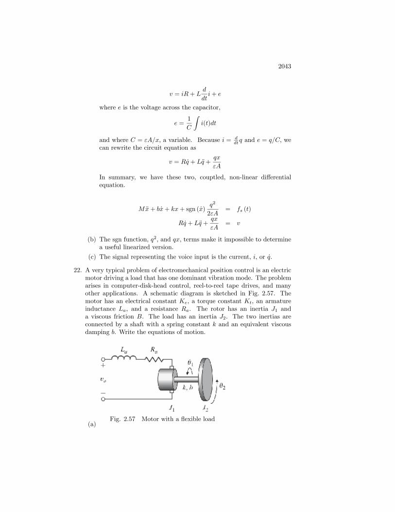
22. A very typical problem of electromechanical position control is an electricmotor driving a load that has one dominant vibration mode. The problemarises in computer-disk-head control, reel-to-reel tape drives, and manyother applications. A schematic diagram is sketched in Fig. 2.57. Themotor has an electrical constant Ke, a torque constant Kt, an armatureinductance La, and a resistance Ra. The rotor has an inertia J1 anda viscous friction B. The load has an inertia J2. The two inertias areconnected by a shaft with a spring constant k and an equivalent viscousdamping b. Write the equations of motion.
(a)Fig. 2.57 Motor with a �exible load

2044 CHAPTER 2. DYNAMIC MODELS
Solution:
(a) Rotor:
J1��1 = �B _�1 � b�_�1 � _�2
�� k (�1 � �2) + Tm
Load:
J2��2 = �b�_�2 � _�1
�� k (�2 � �1)
Circuit:
va �Ke_�1 = La
d
dtia +Raia
Relation between the output torque and the armature current:
Tm = Ktia

2045
23. For the robot in Fig. 2.47, assume you have command of the torque on aservo motor that is connected to the drive wheels with gears that have a2:1 ratio so that the torque on the wheels is increased by a factor of 2 overthat delivered by the servo. Determine the dynamic equations relatingthe speed of the robot with respect to the torque command of the servo.Your equations will require certain quantities, e.g., mass of vehicle, inertiaand radisus of the wheels, etc. Assume you have access to whatever youneed. .
Fig. 2.47 Hospital robot
(a) Solution: First, let�s consider the problem for the case along thelines of the development in Section 2.3.3. That is, a system wherethe torque is applied by a motor on a gear that is simply acceleratingan attached gear, like the picture in Fig. 2.36(b). This basically isassuming that the robot has no mass; but we�ll come back to that.In order to multiply the torque by a factor of 2, the motor must havea gear that is half the size of the gear attached to the wheel, i.e.,n = 2 in Eq. (2.78). For simplicity, let�s also assume there is nodamping on the motor shaft or the wheel shaft, so b1 and b2 are both= 0. If the wheel was not attached to the robot, Eq. (2.78) yields
(Jw + Jmn2)��w = nTm
where Jw = the inertia of the drive wheel, Jm = motor inertia, ��w =wheel angular acceleration, n = 2, and Tm = commanded torque from

2046 CHAPTER 2. DYNAMIC MODELS
the motor. However, the mass of the robot plus all it�s wheels needto be taken into account, since the acceleration of the drive wheel isdirectly related to the acceleration of the robot and its other wheelsprovided there is no slippage. (And, hospital robots probably won�tbe burning rubber ). So that means we need to add the rotationalinertia of the two other wheels and the inertia due to the translationof the cart plus the center of mass of the 3 wheels. The acceleration ofall these quantities are directly related through kinematics because ofthe nonslip assumption. Let�s assume the other two wheels have thesame radius as the drive wheel; therefore, their angular accelerationis also ��w and we�ll also assume they have the same inertia as thedrive wheel. That means, if we neglect the translation inertia of thesystem, the equation becomes
(3Jw + Jmn2)��w = nTm
When you apply a torque to a drive wheel, that torque partly providesan angular accelation of the wheel and the remainder is tranferred tothe contact point as a friction force that accelerates the mass of thevehicle. That friction force is
f = mtota = mtotrw��w
where mtot = the mass of the cart plus all three wheels. By lookingat a FBD of the wheel, we see that the friction force acts as a torque(= rwf) applied to the wheel; and, therefore, it is essentially anotherangular inertia term in the equation above. So the end result is:
(mtotr2w + 3Jw + Jmn
2)��w = nTm
(mtotr2w + 3Jw + 4Jm)
��w = 2Tm
24. Using Fig. 2.36, derive the transfer function between the applied torque,Tm, and the output, �2; for the case when there is a spring attached tothe output load. That is, there is a torque applied to the output load,Ts; where Ts = �Ks�2

2047
Fig. 2.36 (a) geometry de�nitions and forces on teeth (b)de�nitions for the dynamic analysis.
Solution: Equation (2.78), repeated, is
(J2 + J1n2)��2 + (b2 + b1n
2) _�2 = nTm
Since the spring is only applied to the second rotational mass, its torqueonly e¤ects Eq. (2.77). Adding the spring torque to Eq. 2.77 yields
J2��2 + b2 _�2 +Ks�2 = T2
and following the devleopment in the text on page 61, we see that theresult is a revised version of Eq. (2.78), that is
(J2 + J1n2)��2 + (b2 + b1n
2) _�2 +Ks�2 = nTm
Problems and Solutions for Section 2.425. A precision-table leveling scheme shown in Fig. 2.58 relies on thermal
expansion of actuators under two corners to level the table by raising orlowering their respective corners. The parameters are:
Tact = actuator temperature;
Tamb = ambient air temperature;
Rf = heat� ow coe�cient between the actuator and the air;C = thermal capacity of the actuator;
R = resistance of the heater:
Assume that (1) the actuator acts as a pure electric resistance, (2) theheat �ow into the actuator is proportional to the electric power input,and (3) the motion d is proportional to the di¤erence between Tact andTamb due to thermal expansion. Find the di¤erential equations relatingthe height of the actuator d versus the applied voltage vi.

2048 CHAPTER 2. DYNAMIC MODELS
Fig. 2.58 (a) Precision table kept level by actuators; (b) side view ofone actuator
Solution:
Electric power in is proportional to the heat �ow in
_Qin = Kqv2iR
and the heat �ow out is from heat transfer to the ambient air
_Qout =1
Rf(Tact � Tamb) :
The temperature is governed by the di¤erence in heat �ows
_Tact =1
C
�_Qin � _Qout
�=
1
C
�Kqv2iR� 1
Rf(Tact � Tamb)
�and the actuator displacement is
d = K (Tact � Tamb) :
where Tamb is a given function of time, most likely a constant for a tableinside a room. The system input is vi and the system output is d:
26. An air conditioner supplies cold air at the same temperature to each roomon the fourth �oor of the high-rise building shown in Fig. 2.59(a). The �oorplan is shown in Fig. 2.59(b). The cold air �ow produces an equal amountof heat �ow q out of each room. Write a set of di¤erential equationsgoverning the temperature in each room, where
To = temperature outside the building;
Ro = resistance to heat ow through the outer walls;
Ri = resistance to heat ow through the inner walls:

2049
Assume that (1) all rooms are perfect squares, (2) there is no heat �owthrough the �oors or ceilings, and (3) the temperature in each room isuniform throughout the room. Take advantage of symmetry to reduce thenumber of di¤erential equations to three.
Fig. 2.59 Building air conditioning: (a) high-risebuilding, (b) �oor plan of the fourth �oor
Solution:
We can classify 9 rooms to 3 types by the number of outer walls they have.
Type 1 Type 2 Type 1Type 2 Type 3 Type 2Type 1 Type 2 Type 1
We can expect the hotest rooms on the outside and the corners hotest ofall, but solving the equations would con�rm this intuitive result. That is,
To > T1 > T2 > T3
and, with a same cold air �ow into every room, the ones with some sunload will be hotest.
Let�s rede�nce the resistances
Ro = resistance to heat ow through one unit of outer wall
Ri = resistance to heat ow through one unit of inner wall
Room type 1:

2050 CHAPTER 2. DYNAMIC MODELS
qout =2
Ri(T1 � T2) + q
qin =2
Ro(To � T1)
_T1 =1
C(qin � qout)
=1
C
�2
Ro(To � T1)�
2
Ri(T1 � T2)� q
�
Room type 2:
qin =1
Ro(To � T2) +
2
Ri(T1 � T2)
qout =1
Ri(T2 � T3) + q
_T2 =1
C
�1
Ro(To � T2) +
2
Ri(T1 � T2)�
1
Ri(T2 � T3)� q
�
Room type 3:
qin =4
Ri(T2 � T3)
qout = q
_T3 =1
C
�4
Ri(T2 � T3)� q
�
27. For the two-tank �uid-�ow system shown in Fig. 2.59, �nd the di¤erentialequations relating the �ow into the �rst tank to the �ow out of the secondtank.

2051
Fig. 2.60 Two-tank �uid-�ow system for Problem 27
Solution:
This is a variation on the problem solved in Example 2.21 and the de�ni-tions of terms is taken from that. From the relation between the heightof the water and mass �ow rate, the continuity equations are
_m1 = �A1 _h1 = win � w_m2 = �A2 _h2 = w � wout
Also from the relation between the pressure and outgoing mass �ow rate,
w =1
R1(�gh1)
12
wout =1
R2(�gh2)
12
Finally,
_h1 = � 1
�A1R1(�gh1)
12 +
1
�A1win
_h2 =1
�A2R1(�gh1)
12 � 1
�A2R2(�gh2)
12 :
28. A laboratory experiment in the �ow of water through two tanks is sketchedin Fig. 2.61. Assume that Eq. (2.96) describes �ow through the equal-sizedholes at points A, B, or C.
(a) With holes at B and C but none at A, write the equations of motionfor this system in terms of h1 and h2. Assume that when h2 = 15 cm,the out�ow is 200 g/min.
(b) At h1 = 30 cm and h2 = 10 cm, compute a linearized model and thetransfer function from pump �ow (in cubic centimeters per minute)to h2.

2052 CHAPTER 2. DYNAMIC MODELS
(c) Repeat parts (a) and (b) assuming hole B is closed and hole A isopen. Assume that h3 = 20 cm, h1 > 20 cm, and h2 < 20:cm.
Fig. 2.61 Two-tank �uid-�ow system for Problem 28
Solution:
(a) Following the solution of Example 2.21, and assuming the area ofboth tanks is A; the values given for the heights ensure that thewater will �ow according to
WB =1
R[�g (h1 � h2)]
12
WC =1
R[�gh2]
12
WB �WC = �A _h2
Win �WB = �A _h1
From the out�ow information given, we can compute the ori�ce re-sistance, R; noting that for water, � = 1 gram/cc and g = 981cm/sec2 ' 1000 cm/sec2:
WC = 200 g=mn =1
R
p�gh2 =
1
R
p�g � 15 cm
R =
p�g � 10 cm200 g=mn
=
p1 g= cm3 � 1000 cm= s2 � 15 cm
200 g=60 s
=122:5
20060
sg cm2 s2
cm3 s2 g2= 36:7 g�
12 cm�
12

2053
(b) The nonlinear equations from above are
_h1 = � 1
�AR
p�g (h1 � h2) +
1
�AWin
_h2 =1
�AR
p�g (h1 � h2)�
1
�AR
p�gh2
The square root functions need to be linearized about the nominalheights. In general the square root function can be linearized asbelow
px0 + �x =
sx0
�1 +
�x
x0
��=
px0
�1 +
1
2
�x
x0
�So let�s assume that h1 = h10+�h1 and h2 = h20+�h2 where h10 = 30cm and h20 = 10 cm. And for round numbers, let�s assume the areaof each tank A = 100 cm2: The equations above then reduce to
� _h1 = � 1
(1)(100)(36:7)
p(1)(1000) (30 + �h1 � 10� �h2) +
1
(1)(100)Win
� _h2 =1
(1)(100)(36:7)
p(1)(1000) (30 + �h1 � 10� �h2)�
1
(1)(100)(36:7)
p(1)(1000)(10 + �h2)
which, with the square root approximations, is equivalent to,
� _h1 = �p2
36:7(1 +
1
40�h1 �
1
40�h2) +
1
100Win
� _h2 =
p2
36:7(1 +
1
40�h1 �
1
40�h2)�
1
36:7(1 +
1
20�h2)
The nominal in�owWnom =103:67
p2cc/sec is required in order for the
system to be in equilibrium, as can be seen from the �rst equation.So we will de�ne the total in�ow to be Win =Wnom+ �W: Includingthe nominal in�ow, the equations become
� _h1 = �p2
1468(�h1 � �h2) +
1
100�W
� _h2 =
p2
1468�h1 + (
p2
1468� 1
734)�h2 +
p2� 136:7
However, holding the nominal �ow rate maintains h1 at equilibrium,but h2 will not stay at equilibrium. Instead, there will be a con-stant term increasing h2: Thus the standard transfer function willnot result.

2054 CHAPTER 2. DYNAMIC MODELS
(c) With hole B closed and hole A open, the relevant relations are
Win �WA = �A _h1
WA =1
R
p�g(h1 � h3)
WA �WC = �A _h2
WC =1
R
p�gh2
_h1 = � 1
�AR
p�g(h1 � h3) +
1
�AWin
_h2 =1
�AR
p�g(h1 � h3)�
1
�AR
p�gh2
For the value of R, we will use the same calculation from part (a),since that value has not changed with di¤erent hole openings, so westill have
R =122:5
20060
sg cm2 s2
cm3 s2 g2= 36:7 g�
12 cm�
12
. With the same de�nitions for the perturbed quantities as for part(b), plus h3 = 20 cm,.we obtain
� _h1 = � 1
(1)(100)(36:7)
p(1)(1000)(30 + �h1 � 20) +
1
(1)(100)Win
� _h2 =1
(1)(100)(36:7)
p(1)(1000)(30 + �h1 � 20)
� 1
(1)(100)(36:7)
p(1)(1000)(10 + �h2)
which, with the linearization carried out, reduces to
� _h1 = � 1
(36:7)(1 +
1
20�h1) +
1
(100)Wnom +
1
(100)�W
� _h2 =1
(36:7)(1 +
1
20�h1)�
1
(36:7)(1 +
1
20�h2)
and with the nominal �ow rate of Win =103:67 removed
� _h1 = � 1
734�h1 +
1
100�W
� _h2 =1
734�h1 �
1
734�h2

2055
Taking the Laplace transform of these two equations, and solving forthe desired transfer function (in cc/sec) yields
�H2(s)
�W (s)=
1
734
0:01
(s+ 1=734)2:
which becomes, with the in�ow in grams/min,
�H2(s)
�W (s)=
1
734
(0:01)(60)
(s+ 1=734)2= :
0:000817
(s+ 1=734)2
29. The equations for heating a house are given by Eqs. (2.81) and (2.82)and, in a particular case can be written with time in hours as
CdThdt
= Ku� Th � ToR
where
(a) C is the Thermal capacity of the house, BTU=oF
(b) Th is the temperature in the house, oF
(c) To is the temperature outside the house, oF
(d) K is the heat rating of the furnace, = 90; 000 BTU=hour
(e) R is the thermal resistance, oF per BTU=hour
(f) u is the furnace switch, =1 if the furnace is on and =0 if the furnaceis o¤.
It is measured that, with the outside temperature at 32 oF and the houseat 60 oF , the furnace raises the temperature 2 oF in 6 minutes (0.1hour). With the furnace o¤, the house temperature falls 2 oF in 40minutes. What are the values of C and R for the house?
Solution:
For the �rst case, the furnace is on which means u = 1.
CdThdt
= K � 1
R(Th � To)
_Th =K
C� 1
RC(Th � To)
and with the furnace o¤,
_Th = �1
RC(Th � To)
In both cases, it is a �rst order system and thus the solutions involveexponentials in time. The approximate answer can be obtained by simply

2056 CHAPTER 2. DYNAMIC MODELS
looking at the slope of the exponential at the outset. This will be fairlyaccurate because the temperature is only changing by 2 degrees and thisrepresents a small fraction of the 30 degree temperature di¤erence. Let�ssolve the equation for the furnace o¤ �rst
�Th�t
= � 1
RC(Th � To)
plugging in the numbers available, the temperature falls 2 degrees in 2/3hr, we have
� 2
2=3= � 1
RC(60� 32)
which means thatRC = 28=3
For the second case, the furnace is turned on which means
�Th�t
=K
C� 1
RC(Th � To)
and plugging in the numbers yields
2
0:1=90; 000
C� 1
28=3(60� 32)
and we have
C =90; 000
23= 3913
R =RC
C=28=3
3913= 0:00239
Feedback Control of Dynamic Systems 8th Edition Franklin Solutions ManualFull Download: https://alibabadownload.com/product/feedback-control-of-dynamic-systems-8th-edition-franklin-solutions-manual/
This sample only, Download all chapters at: AlibabaDownload.com