fem_modeling_project_evaluation of a steel pulley and shaft design
TRANSCRIPT

City College of New York School of Engineering
Mechanical Engineering Department
Spring-2014
Mechanical Engineering I 6500: Computer-Aided Design Instructor : Prof. Gary Benenson
Student : Mehmet Bariskan
FEM Modeling Project #2 : Evaluation of a Steel Pulley and
Shaft Design

2
Overview
A pulley is a wheel on an axle that is designed to support movement and change of direction of a
cable or belt along its circumference. Pulleys are used in a variety of ways to lift loads, apply
forces, and to transmit power. The drive element of a pulley system can be a rope, cable, belt, or
chain that runs over the pulley inside the groove.
In this project, we are asked to evaluate the design of a machine part. The part is a steel pulley
with attached shaft, shown below in Figure 1. The shaft is connected to a motor, which continues
attempting to turn, even though an obstacle has penetrated one of the holes, preventing an inside
face from moving. The primary purpose of the analysis is to determine whether the pulley-shaft
system would deform permanently under these circumstances. If it does, my task will be to
redesign it to prevent this failure.
Figure 1: A Steel Pulley with the Attached Shaft
Procedure
1. The First Approximation
We are given the solid part of the pulley with attached shaft and its boundary conditions for
further analysis. I have defined the material composition as AISI 1020 steel and cold rolled. The
yield strength of this material is approximately 350 MPa.
Firstly, I have applied a torque of 100 N-m to the outer face of the shaft. The line labeled “Axis
1” was used for the direction of the torque. The torque vector is always perpendicular to the
directions of the forces causing the torque, according to the given information. Secondly, I have
3
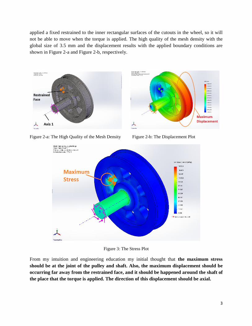
applied a fixed restrained to the inner rectangular surfaces of the cutouts in the wheel, so it will
not be able to move when the torque is applied. The high quality of the mesh density with the
global size of 3.5 mm and the displacement results with the applied boundary conditions are
shown in Figure 2-a and Figure 2-b, respectively.
Figure 2-a: The High Quality of the Mesh Density Figure 2-b: The Displacement Plot
Figure 3: The Stress Plot
From my intuition and engineering education my initial thought that the maximum stress
should be at the joint of the pulley and shaft. Also, the maximum displacement should be
occurring far away from the restrained face, and it should be happened around the shaft of
the place that the torque is applied. The direction of this displacement should be axial.

4
The maximum stress of the initial condition was in the small rectangular box where we have
applied a fixed restrained in the first approximation which is invalid that is shown in Figure 3.
Also, this study shows that the area of the wheel, contrary to fixed restrained is where the
maximum displacement is located but not on the shaft which is shown in Figure 2-b. These plots
show that the given boundary conditions are not valid. These boundary conditions reflect the
behavior of pulleys would be allowed to move towards and away from any adjacent pulley and
would therefore not be able to transmit a force to its belt.
2. The Second Approximation with the Customized Boundary Conditions
The next step was to customize the given boundary condition. At first, I have applied a fixed
restraint at the small rectangular box and torque of 100 N-m on the outer shaft face. I have added
a fixed hinge at the face of the shaft that will allow the shaft to rotate anti-clockwise with the
pulley fixed only the shaft moving the customized boundary condition is shown in Figure 4.
Figure 4: The Customized Boundary Conditions
After the first run of the simulation study of the pulley, I have observed that the maximum stress at the
joint of the pulley and shaft as I expected that is shown in Figure 5. After then, I have observed that the
maximum displacement was occurring at the place where the torque is applied that was I expected also
which is shown in Figure 6.

5
Figure 5: The Maximum Stress for the new boundary conditions
.
Figure 6: The Maximum Displacement for the new boundary conditions
Evaluation of the Design
The yield strength of the given material is 350Mpa and FOS (Factor of safety) is 2. Therefore, my first
concern is to observe the maximum stress, which we will get from our studies should not exceed the half
of the yield strength. The Von-mises stress we get from the plot should be less than 175Mpa because it
should be lower than the half of the yield stress.
, 2 is a constant for the factor of safety

6
Now it is time to find the maximum stress value for this model. To get an accurate result, I have used the
different element sizes for global and local mesh. The local mesh was applied to the joint of the pulley
and the shaft which is shown in Figure 7.
Figure 7: Local mesh control
After performing the first mesh study, we could see that the maximum stress value is higher than the
maximum allowable stress value. The tabulated data and a convergence study are shown in Table 1 and
Figure 8, respectively.
Mesh Density
& Quality
Maximu
m Stress
(MPa)
Maximum
Displacement
(µm)
Total
# of
Element
Total
# of
Nodes
Total
# of
DOF
Global
Element
Size (mm)
Location(s)
Local
Refinement
Size (mm)
Running
Time
(second)
1a-Coarse Mesh
65.28 26.58 2818 5236 15663 14 N/A 1
1b- Medium Mesh
68.81 26.39 8989 15333 45906 7 N/A 2
1c-Fine Mesh
91.90 26.17 55776 85181 255282 3.5 N/A 12
1d-Fine Mesh
93.06 26.14 373179 539312 1617051 1.75 N/A 44
1e-Fine Mesh 96.92 26.16 391230 563581 1690158 1.75 1 42
1f-Fine Mesh 125.93 26.18 430420 616466 1848513 1.75 0.5 49
1g-Fine Mesh 165.62 26.19 501501 713085 2138370 1.75 0.25 62
1h-Fine Mesh 233.52 26.20 626280 883641 2650038 1.75 0.12 94
Table 1: Tabulated Data from SolidWorks Simulation

7
Figure 8: Maximum Stress versus Number of Degrees of Freedom for the given model
Since the maximum stress value is higher than the maximum allowable stress. I have changed the
design of the model to reduce this stress. Firstly, I have added a fillet of 1 mm at the joint of the
pulley and shaft. Then, I have tried different size of radius to get the optimum fillet radius
Mesh Density
& Quality Fillet = 1 mm
Maximu
m Stress
(MPa)
Maximum
Displacement
(µm)
Total
# of
Element
Total
# of
Nodes
Total
# of
DOF
Global
Element
Size (mm)
Location(s)
Local
Refinement
Size (mm)
Running
Time
(second)
2a- Coarse Mesh
104.17 26.61 3108 5645 16890 14 N/A 1
2b- Medium Mesh
111.36 26.45 9275 15746 47145 7 N/A 1
2c-Fine Mesh
112.43 26.19 56931 86742 259965 3.5 N/A 5
2d-Fine Mesh
118.81 26.13 378336 546356 1638183 1.75 N/A 44
Table 2: Tabulated Data for the fillet radius= 1 mm
Mesh Density
& Quality Fillet = 2 mm
Maximu
m Stress
(MPa)
Maximum
Displacement
(µm)
Total
# of
Element
Total
# of
Nodes
Total
# of
DOF
Global
Element
Size (mm)
Location(s)
Local
Refinement
Size (mm)
Running
Time
(second)
2e- Coarse Mesh
86.52 26.47 3020 5528 16539 14 N/A 1
2f- Medium Mesh
91.03 26.37 9373 15878 47541 7 N/A 1
2g-Fine Mesh
92.66 26.08 56394 85978 257673 3.5 N/A 5
2h-Fine Mesh
98.74 26.05 375986 543241 1628838 1.75 N/A 41
Table 3: Tabulated Data for the fillet radius= 2 mm
0
50
100
150
200
250
0 500000 1000000 1500000 2000000 2500000 3000000
Max
imu
m S
tre
ss [
MP
a]
Number of degrees of freedom
Max. Stress & DOF
Max. Stress (Mpa)

8
Mesh Density
& Quality Fillet = 3 mm
Maximu
m Stress
(MPa)
Maximum
Displacement
(µm)
Total
# of
Element
Total
# of
Nodes
Total
# of
DOF
Global
Element
Size (mm)
Location(s)
Local
Refinement
Size (mm)
Running
Time
(second)
2i- Coarse Mesh
83.74 26.41 3219 5821 17418 14 N/A 1
2j Medium Mesh
83.73 26.22 9551 16115 48252 7 N/A 1
2k-Fine Mesh
86.41 25.94 55414 84646 253677 3.5 N/A 5
2l-Fine Mesh
106.42 25.92 406278 583566 1749813 1.75 N/A 37
Table 4: Tabulated Data for the fillet radius= 3 mm
Mesh Density
& Quality Fillet = 5 mm
Maximu
m Stress
(MPa)
Maximum
Displacement
(µm)
Total
# of
Element
Total
# of
Nodes
Total
# of
DOF
Global
Element
Size (mm)
Location(s)
Local
Refinement
Size (mm)
Running
Time
(second)
2m- Coarse Mesh
69.57 26.05 3150 5726 17133 14 N/A 1
2n- Medium Mesh
72.44 25.87 9234 15680 46947 7 N/A 1
2o-Fine Mesh
81.18 25.65 53887 82597 247530 3.5 N/A 4
2p-Fine Mesh
93.06 25.62 395153 568495 1704600 1.75 N/A 36
Table 5: Tabulated Data for the fillet radius= 5 mm
Secondly, I have changed the shaft diameter from 25 mm to 30 mm. I have chosen the fillet
radius of 5 mm. The tabulated data for both studies are shown in from Table 6 to Table 9.

9
Mesh Density
Standard Fillet = 5 mm
Shaft D. = 25 mm
Maximu
m Stress
(MPa)
Maximum
Displacement
(µm)
Total
# of
Element
Total
# of
Nodes
Total
# of
DOF
Global
Element
Size
(mm)
Location(s)
Local
Refinement
Size (mm)
Running
Time
(second)
3-a 81.18 25.65 53887 82597 247530 3.5 N/A 4
3-b 83.28 25.66 101595 150286 450543 3 N/A 8
3-c 88.54 25.64 153758 226041 677616 2.5 N/A 15
3-d 90.39 25.63 280902 406980 1220175 2 N/A 27
3-e 99.60 25.62 561405 805298 2414679 1.5 N/A 58
3-f 101.02 25.62 908684 1293196 4293196 1.25 N/A 104
3-g 112.42 25.62 1664862 2347122 7038825 1 N/A 355
Table 6: Tabulated Data for the fillet radius = 5 mm and the shaft diameter = 25 mm (Using the
Standard Based Mesh Function)
Figure 9: Maximum Stress versus Number of Degrees of Freedom for the fillet radius = 5 mm and
the shaft diameter = 25 mm
0
20
40
60
80
100
120
0 1000000 2000000 3000000 4000000 5000000 6000000 7000000 8000000
Max
imu
m S
tre
ss [
MP
a]
Number of degrees of freedom
Max. Stress & DOF
Max. Stress (Mpa)

10
Curvature
Based Fillet = 5 mm
Shaft D. = 25 mm
Maximu
m Stress
(MPa)
Maximum
Displacement
(µm)
Total
# of
Element
Total
# of
Nodes
Total
# of
DOF
Global
Element
Size
(mm)
Location(s)
Local
Refinement
Size (mm)
Running
Time
(second)
3-h 83.18 25.70 86818 130190 390123 3.5 N/A 9
3-i 84.52 25.70 121802 181478 544041 3 N/A 11
3-j 101.04 25.68 166952 246805 739668 2.5 N/A 16
3-k 111.20 25.63 366137 529154 1586619 2 N/A 34
3-l 110.72 25.62 773890 1104698 3313035 1.5 N/A 78
3-m 111.35 25.62 1082558 1538783 4613850 1.25 N/A 105
3-n 123.80 25.62 2083156 2934283 8799582 1 N/A 442
Table 7: Tabulated Data for the fillet radius = 5 mm and the shaft diameter = 25 mm (Using the
Curvature Based Mesh Function)
Figure 10: Maximum Stress versus Number of Degrees of Freedom for the fillet radius = 5 mm
and the shaft diameter = 25 mm
0
20
40
60
80
100
120
140
0 2000000 4000000 6000000 8000000 10000000
Max
imu
m S
tre
ss [
MP
a]
Number of degrees of freedom
Max. Stress & DOF
Max. Stress (Mpa)

11
Standart Based Fillet = 5 mm
Shaft D. = 30 mm
Maximu
m Stress
(MPa)
Maximum
Displaceme
nt
(µm)
Total
# of
Element
Total
# of
Nodes
Total
# of
DOF
Global
Element
Size
(mm)
Location(s)
Local
Refinement
Size (mm)
Running
Time
(second)
3-o 51.46 15.61 55770 85235 255444 3.5 N/A 5
3-p 53.61 15.61 91317 136709 409812 3 N/A 9
3-r 54.29 15.60 129975 192971 578466 2.5 N/A 12
3-s 58.27 15.61 264231 385429 1155522 2 N/A 24
3-t 65.46 15.61 554605 796975 2389710 1.5 N/A 50
3-u 68.46 15.61 921353 1311111 3931590 1.25 N/A 98
3-v 75.87 15.61 1701552 2397530 7190049 1 N/A 431
Table 8: Tabulated Data for the fillet radius = 5 mm and the shaft diameter = 30 mm (Using the
Standard Mesh Function)
Figure 11: Maximum Stress versus Number of Degrees of Freedom for the fillet radius = 5 mm
and the shaft diameter = 30 mm
0
10
20
30
40
50
60
70
80
0 1000000 2000000 3000000 4000000 5000000 6000000 7000000 8000000
Max
imu
m S
tre
ss [
MP
a]
Number of degrees of freedom
Max. Stress & DOF
Max. Stress (Mpa)

12
Curvature
Based Fillet = 5 mm
Shaft D. = 30 mm
Maximu
m Stress
(MPa)
Maximum
Displaceme
nt
(µm)
Total
# of
Element
Total
# of
Nodes
Total
# of
DOF
Global
Element
Size
(mm)
Location(s)
Local
Refinement
Size (mm)
Running
Time
(second)
3-y 58.77 15.64 87581 131446 393987 3.5 N/A 9
3-x 62.28 14.32 122927 183124 548925 3 N/A 12
3-aa 61.92 15.61 167204 247421 741552 2.5 N/A 16
3-ab
71.26 15.61 362183 523985 1571124 2 N/A 34
3-ac 73.07 15.61 789946 1127207 3380514 1.5 N/A 84
3-ad 80.48 15.61 1054983 1501506 4502043 1.25 N/A 110
3-ae 89.06 15.62 2096736 2953341 8856780 1 N/A 477
Table 9: Tabulated Data for the fillet radius = 5 mm and the shaft diameter = 30 mm (Using the
Curvature Based Mesh Function)
Figure 12: Maximum Stress versus Number of Degrees of Freedom for the fillet radius = 5 mm
and the shaft diameter = 30 mm
0
10
20
30
40
50
60
70
80
90
100
0 2000000 4000000 6000000 8000000 10000000
Max
imu
m S
tre
ss [
MP
a]
Number of degrees of freedom
Max. Stress & DOF
Max. Stress (Mpa)

13
3. The Third Approximation with the Customized Boundary Conditions
After, I had completed the studies of the first customized boundary conditions. I have observed
that they are not converging. When I consider the real part under the working conditions, I have
thought to change the fixed restraint place from the face of the small rectangular box to around
the wheel where the belt can force the part to turn. The second customized boundary conditions
are shown in Figure 13.
Figure 13: The Second Customized Boundary Conditions
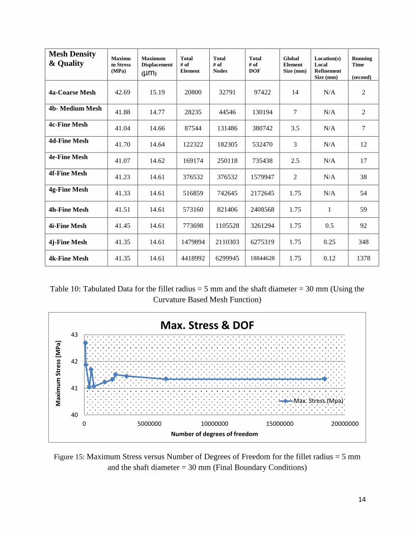
To get an accurate result and to save time for the process, I have used the different element sizes for
global and local mesh. The local mesh was applied to the joint section that is shown in Figure 14. The
mesh study is shown in Table 10.
Figure 14: Local mesh control for second customized boundary conditions
14
Mesh Density
& Quality
Maximu
m Stress
(MPa)
Maximum
Displacement
(µm)
Total
# of
Element
Total
# of
Nodes
Total
# of
DOF
Global
Element
Size (mm)
Location(s)
Local
Refinement
Size (mm)
Running
Time
(second)
4a-Coarse Mesh
42.69 15.19 20800 32791 97422 14 N/A 2
4b- Medium Mesh
41.88 14.77 28235 44546 130194 7 N/A 2
4c-Fine Mesh
41.04 14.66 87544 131486 380742 3.5 N/A 7
4d-Fine Mesh
41.70 14.64 122322 182305 532470 3 N/A 12
4e-Fine Mesh
41.07 14.62 169174 250118 735438 2.5 N/A 17
4f-Fine Mesh
41.23 14.61 376532 376532 1579947 2 N/A 38
4g-Fine Mesh
41.33 14.61 516859 742645 2172645 1.75 N/A 54
4h-Fine Mesh 41.51 14.61 573160 821406 2408568 1.75 1 59
4i-Fine Mesh 41.45 14.61 773698 1105528 3261294 1.75 0.5 92
4j-Fine Mesh 41.35 14.61 1479894 2110303 6275319 1.75 0.25 348
4k-Fine Mesh 41.35 14.61 4418992 6299945 18844628 1.75 0.12 1378
Table 10: Tabulated Data for the fillet radius = 5 mm and the shaft diameter = 30 mm (Using the
Curvature Based Mesh Function)
Figure 15: Maximum Stress versus Number of Degrees of Freedom for the fillet radius = 5 mm
and the shaft diameter = 30 mm (Final Boundary Conditions)
40
41
42
43
0 5000000 10000000 15000000 20000000
Max
imu
m S
tre
ss [
MP
a]
Number of degrees of freedom
Max. Stress & DOF
Max. Stress (Mpa)

15
Discussion
The resulting stress due to the given boundary conditions was in the hole of the wheel in the first
analysis. My prediction was at the joint of the shaft and pulley. The maximum displacement due
to given boundary conditions was around the wheel in the first analysis. My prediction was at the
place where the torque is applied. After, I see the displacement plot that is Figure 2-b. I have
decided to add a new boundary condition to prevent the shaft center to move. I have chosen the
fixed-hinge function and it’s prevented to move the shaft from the its center.
Secondly, I have continued with a convergence study to find a solution, unfortunately study was
not converging that is shown in Table 1 and Figure 8. As we see section 2, I have added a fillet
to joint of the shaft and pulley. Then, I have changed the shaft diameter to decrease the
maximum stress for the design. Even though, they had helped the decrease the stress in the
customized design, I couldn’t trust the solution because of the convergence study has failed.
Finally, I have decided to change the place of the fixed-restraint from one of the faces of the hole
of the wheel to around of the wheel that is shown in Figure 13. That solved the problem of the
convergence study. The final results are shown in Table 10 and Figure 15.
The maximum stress is approximately 41 MPa that is safe for the given material. The part does
not fail, thus it does not permanently deform.
A lot was learned through the path of this assignment. While the first project for the FEM
analysis gave us more outcome of how particular mesh refinement and location has it on results.
Whereas, this project was more about applying the different boundary conditions, and
customizing the geometry to get an intended result. One thing which impressed me is using
different boundary conditions which had given an accurate result. Overall the assignment gave a
sense of solving a real life problem.