Optimal Fiscal Policy in a Small Open Economy with

Limited Commitment∗

Sofia Bauducco†

Central Bank of Chile

Francesco Caprioli‡

Banca d’Italia

December 2010

Abstract

We introduce limited commitment into a standard optimal fiscal policy model in open

economies. We consider the problem of a benevolent government that signs a risk-sharing

contract with the rest of the world, and that has to choose optimally distortionary taxes on

labor income, domestic debt and international debt. Both the home country and the rest of

the world have limited commitment, which means that they can leave the contract if they

find this convenient. The contract is designed so that, at any point in time, neither party

has incentives to exit. Our model is able to rationalize two stylized facts about fiscal policy

in emerging economies: i) the volatility of tax revenues over GDP is positively correlated

with sovereign default risk; ii) fiscal policy is procyclical. The first fact is novel, while the

second fact has been well documented in the literature. In contrast with previous work, we

show that only a small deviation from complete markets is needed to generate this result.

∗We would like to thank Albert Marcet for constant encouragement and guidance. We also benefited from fruit-ful discussions with Alexis Anagnostopoulos, Fabio Canova, Miguel Fuentes, Juan Pablo Nicolini, Eva Carceles-Poveda, Begona Dominguez, Jordi Galı, Alexandre Janiak, Patrick Kehoe, Stefano Neri, Michael Reiter, JaumeVentura and seminar participants at the UPF Macro Break, XII Spring Meeting of Young Economists, EEA- ESEM 2007 Congress, ASSET 2007 Conference, 32 Simposio de Analisis Economico, La Pietra-MondragoneWorkshop 2008, CEA Universidad de Chile, USACH, FEN Universidad de Chile, Central Bank of Chile andLACEA 2010 Conference. All remaining errors are our own.

†Corresponding author. Email: sbauducco@bcentral.cl‡Email: francesco.caprioli@upf.edu

1

1 Introduction

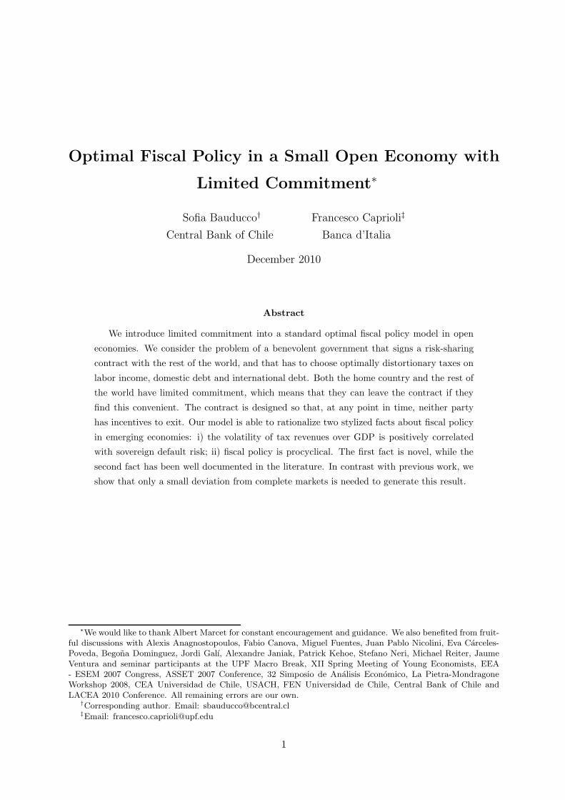
Table 1 shows some statistics for government expenditure and tax revenues as a percentage

of GDP in Argentina and in the USA. The table shows two remarkable features. First, the

sample means of the government expenditure and tax revenues processes for both countries are

very similar. Second, although the variability of the government expenditure series is roughly

the same in the two countries, tax revenues in Argentina are much more volatile than in the

USA: the standard deviation of the series for Argentina is almost 60% higher than the one for

the US economy.

Table 1: Fiscal variables for the USA and Argentina

USA Argentina

Govt. expend Tax revenues Govt. expend. Tax revenues(as % of GDP) (as % of GDP) (as % of GDP) (as % of GDP)

Mean 17.55 18.50 17.04 18.28St. deviation 0.92 1.30 0.98 2.14

Coef. of variation 0.0525 0.0704 0.0573 0.117

Note: The series for USA are from the Bureau of Economic Analysis of the US Department of Commerce. In the caseof Argentina, the data we use is from the IMF, INDEC and Ministerio de Economia. We use quarterly data of currentgovernment expenditure net of interest payments plus gross government investment as a measure of government expenditure,and total tax revenues plus contributions to social security as a measure of total tax revenues. The sample period is1993 − 2005.

This evidence seems to be at odds with a standard model of optimal fiscal policy in a small

open economy a la Lucas and Stokey (1983). Consider a setup in which a small open economy,

which we call the home country, can trade assets with the rest of the world. The government of

the home country has to collect revenues optimally in order to finance an exogenous stream of

public expenditure. In this case, a benevolent government of the home country would set taxes

roughly constant over the business cycle. When a bad shock hits the economy, the government

can borrow from abroad and pay back the debt later on, when the economy faces instead a good

shock. In this way, the possibility to do risk-sharing with the rest of the world implies that the

deadweight losses associated to distortionary taxation are minimized1. It follows that, at least

from a theoretical point of view, tax volatility in small open economies should be lower than

tax volatility in large or closed economies, thanks to the insurance role played by international

borrowing and lending.

In this paper we introduce sovereign default risk into a standard optimal fiscal policy open

economy model as the one described before by relaxing the assumption of full commitment from

the home country and the rest of the world towards their contracted obligations. We show that

1As we show in Section 3.5.1, in the extreme case in which the rest of the world is risk neutral, the optimaltax rate is perfectly flat and all fluctuations in public expenditure can be absorbed by international capital flows.

2

this framework provides a theoretical justification for the tax rate volatility observed in emerging

small open economies that have commitment problems to repay their external obligations.

In the model, the home country is populated by risk adverse households. The fiscal authority

has to finance an exogenous public expenditure shock either through distortionary labor income

taxes or by issuance of internal and/or international debt. The rest of the world is inhabited by

risk-neutral agents that receive a constant endowment and have to decide how much to consume

and how much to borrow/lend in the international capital market. We assume that there is

limited commitment, in the sense that neither the government in the home country nor the rest

of the world can commit to pay back the debt contracted among themselves.

A contract, signed by the two countries, regulates international capital flows. The terms of

the contract depend on the commitment technology available to the two parts to honor their

external obligations. When both countries can fully commit to stay in the contract in all states

of nature, the only condition to be met is that ex-ante there is no exchange of net wealth among

them. Instead, when the countries may at some point decide to leave the contract, further

conditions need to be imposed. In particular, since default takes place if the benefit a country

obtains from staying in the contract is smaller than its outside option, the contract must specify

an adjustment in the allocation necessary to rule out default in equilibrium.

We show that the presence of sovereign default risk, i.e., the possibility that a country may

exit the contract with the other country, limits the amount of risk-sharing among countries.

Consequently, the classical tax-smoothing result is dampened since now the optimal tax rate

depends on the incentives to default of both countries. Specifically, when a large government

expenditure shock hits the home country, a fraction of this expenditure has to be absorbed by

tax revenues, and this fraction increases, the stronger the commitment problem is.

An important corollary of our analysis is that optimal fiscal policy in the presence of limited

commitment should be procyclical. A (large) negative shock should be met by an increase in

tax rates, and the converse holds for a (large) positive shock. We study the robustness of this

assertion shutting down shocks to government expenditure and introducing productivity shocks.

Our exercise suggests that a small deviation from full commitment is sufficient to turn fiscal

policy from strongly countercyclical to procyclical. This result is in line with recent empirical

evidence on the cyclical properties of fiscal policy for emerging economies, as Gavin and Perotti

(1997), Kaminsky et al. (2004), Talvi and Vegh (2005) and Ilzetzki and Vegh (2008).

Some papers, such as Riascos and Vegh (2003) and Cuadra et al. (2010), relate the procycli-

cality of fiscal policy in emerging economies to the presence of market incompleteness in analyses

of optimal policy. However, these studies assume extreme cases of market incompleteness, as

they consider that the government only has access to a one-period non contingent bond. We

show that even slight degrees of market incompleteness are sufficient to deliver the result2.

2As will be clear from the analysis of the following sections, a departure from the full commitment assumption

3

Alternative explanations for the high volatility of tax rates observed in emerging economies

rely on the quality of their institutions and the sources of tax collection. It is argued that

emerging countries are more prone to switches in political and economic regimes that, almost

by definition, translate into unstable tax systems. Moreover, in booms these countries often tax

heavily those economic sectors that are responsible for the higher economic activity3. As a con-

sequence, when economic conditions deteriorate, necessarily tax revenues go down dramatically.

We are aware that these considerations are relevant sources of tax variability and that our study

does not incorporate them in the analysis. However, we do not intend to provide an exhaustive

description of such sources, but rather to focus on sovereign risk and incomplete international

capital markets as possible causes for the high tax rate volatility of emerging economies.

In the recent years there have been some attempts to add default to dynamic macroeconomic

models. A number of papers (Arellano (2008), Aguiar and Gopinath (2006)) have introduced

sovereign default in otherwise standard business cycle models in order to quantitatively match

some empirical regularities of small open emerging economies. More specifically, they adapt the

framework of Eaton and Gersovitz (1981) to a dynamic stochastic general equilibrium model.

These models are usually able to explain with relative success the evolution of the interest rate,

current account, output, consumption and the real exchange rate. Nevertheless, since they all

consider endowment economies, they fail to capture the effects of default risk over the taxation

scheme. Moreover, in these models the government issues one-period non contingent defaultable

debt. Our contribution is to extend the analysis to be able to characterize the shape of fiscal

policy and the links between the risk of default and taxes in a limited commitment framework.

To do so, rather than assuming extreme forms of market incompleteness as these papers do,

we consider a small deviation from complete markets. The reason for this is that we want to

provide the government with as many instruments as possible to smooth tax rates.

Several papers have introduced the idea of limited commitment to study many important

issues. Among others, Kehoe and Perri (2002) introduce credit arrangement between countries

to reconcile international business cycle models with complete markets and the data, Krueger

and Perri (2006) look at consumption inequality, Chien and Lee (2010) look at capital taxation

in the long-run, Marcet and Marimon (1992) study the evolution of consumption, investment

and output, and Kocherlakota (1996) analyzes the properties of efficient allocations in a model

with symmetric information and two-sided lack of commitment. To our knowledge, none of them

has focused on the impact of the possibility of default on the volatility of optimal taxation and

the cyclical properties of fiscal policy.

The closest papers to ours are probably those by Cuadra et al. (2010), Pouzo (2008) and

in our framework implies that international financial markets are endogenously incomplete.3As an example, in the recent years Argentina has been experiencing rapid export-led growth, mainly due to

exports of commodities such as soya. In this period, the government’s main source of tax revenues has come fromtaxation of these exports.

4

Scholl (2009). The first paper focuses on matching some stylized facts in emerging countries,

namely the positive correlation between risk premia and the level of external debt, higher risk

premia during recessions and the procyclicality of fiscal policy in emerging economies. The sec-

ond paper studies the optimal taxation problem in a closed economy under incomplete markets

allowing for default on internal debt. Finally, the third paper analyzes the problem of a donor

that has to decide how much aid to give to a government that has an incentive to use these

external resources to increase its own personal consumption without decreasing the distortive

tax income it levies on private agents.

We differentiate from these papers along various dimensions. We consider the full commit-

ment solution instead of the time-consistent one. We do this to isolate the effect of endogenously

incomplete markets on the optimal fiscal plan, while giving the government all the usual tools

to distribute the burden of taxation across periods and states of the world. In particular, in

our framework there is a complete set of state-contingent bonds the government can issue inter-

nally. This has important implications for consumption smoothing as it allows the government

to distribute the burden of taxation across states. Finally, in contrast with the assumption in

Scholl (2009), we focus on the scenario in which the government of the small open economy is

benevolent, i.e., its objective is to maximize the expected life-time utility of its citizens.

The rest of the paper proceeds as follows. Complementing Table 1, Section 2 provides some

evidence on the positive correlation between sovereign risk and volatility of tax revenues as a

fraction of GDP. Section 3 describes the model. Section 4 shows how the optimal fiscal plan is

affected by the the presence of limited commitment in the case study of a perfectly anticipated

one-time fiscal shock. In Section 5 we solve the model for the general case of an autocorrelated

government expenditure shock. The cyclical properties of the optimal fiscal policy plan when

there is limited commitment are analyzed in Section 6. Section 7 is devoted to show that our

economy can be reinterpreted as one in which the government can issue debt subject to debt

limits, both on internal and external debt. Section 8 concludes.

2 Stylized facts

In this section we present some evidence showing that the volatility of tax revenues over

GDP of a country is correlated with the country’s risk premium. We base our analysis on these

variables because, in the following sections, we develop a model to explain these facts by linking

the volatility of tax rates to the lack of commitment of a country towards its foreign liabilities4.

We use annual data on tax revenues over GDP, total government expenditure over GDP

4In the model depicted in the next sections, the marginal tax rate is equal to tax revenues over GDP. Althoughthis identity is due to the specific tax structure and production function considered, due to data unavailabilitywe cannot obtain marginal tax rates for the countries for which we perform the analysis. Consequently, we taketax revenues over GDP to be the best proxy available for marginal tax rates.

5

!"!!#

!"!$#

!"!%#

!"!&#

!"!'#

!"(!#

!"($#

!"(%#

!"(&#

!"('#

!# !"!)# !"(# !"()# !"$# !"$)#

!"#$%&"$&'()*(+",&"$&-(.&)#'#,/#01234&

5#(,&65782&09)#(:&

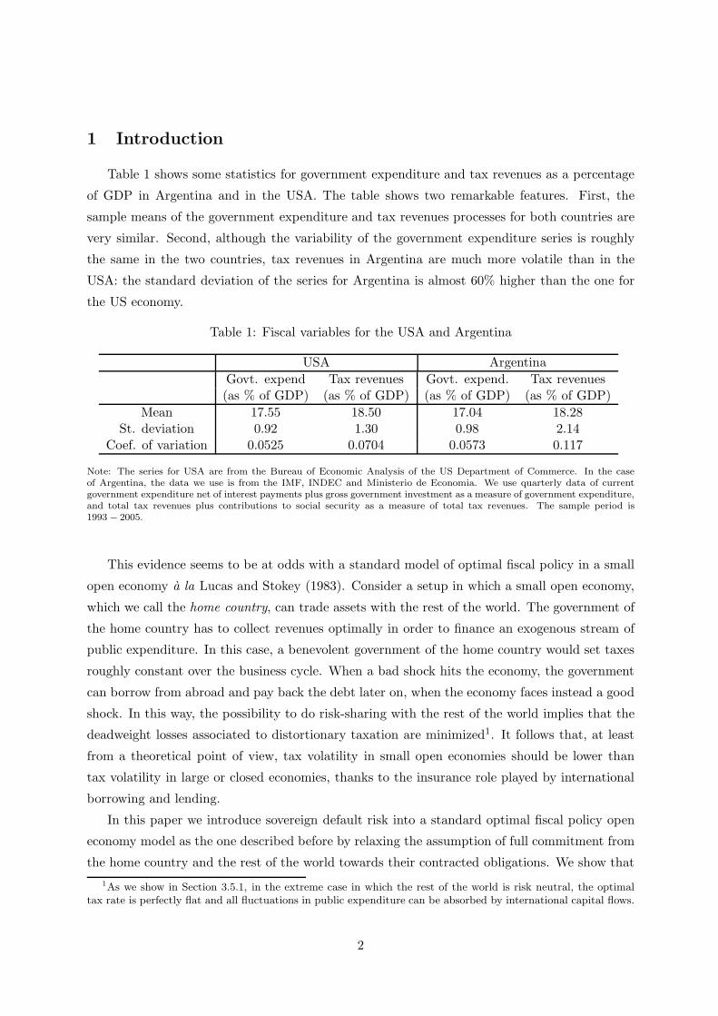
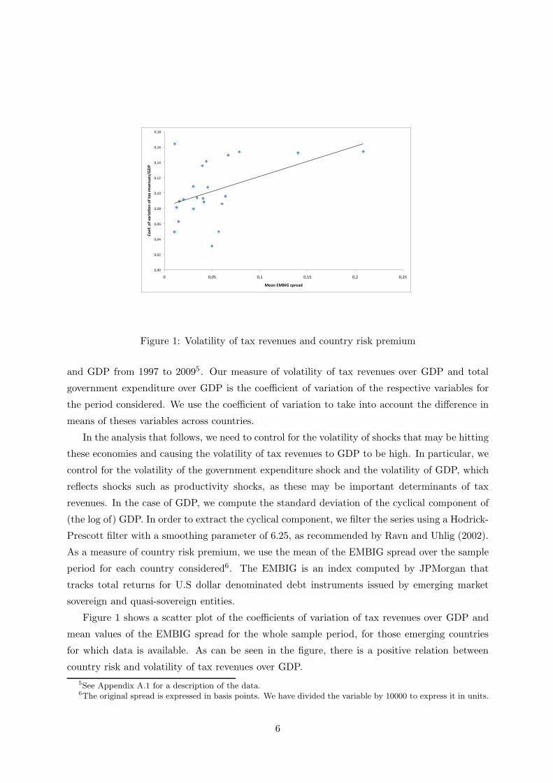
Figure 1: Volatility of tax revenues and country risk premium

and GDP from 1997 to 20095. Our measure of volatility of tax revenues over GDP and total

government expenditure over GDP is the coefficient of variation of the respective variables for

the period considered. We use the coefficient of variation to take into account the difference in

means of theses variables across countries.

In the analysis that follows, we need to control for the volatility of shocks that may be hitting

these economies and causing the volatility of tax revenues to GDP to be high. In particular, we

control for the volatility of the government expenditure shock and the volatility of GDP, which

reflects shocks such as productivity shocks, as these may be important determinants of tax

revenues. In the case of GDP, we compute the standard deviation of the cyclical component of

(the log of) GDP. In order to extract the cyclical component, we filter the series using a Hodrick-

Prescott filter with a smoothing parameter of 6.25, as recommended by Ravn and Uhlig (2002).

As a measure of country risk premium, we use the mean of the EMBIG spread over the sample

period for each country considered6. The EMBIG is an index computed by JPMorgan that

tracks total returns for U.S dollar denominated debt instruments issued by emerging market

sovereign and quasi-sovereign entities.

Figure 1 shows a scatter plot of the coefficients of variation of tax revenues over GDP and

mean values of the EMBIG spread for the whole sample period, for those emerging countries

for which data is available. As can be seen in the figure, there is a positive relation between

country risk and volatility of tax revenues over GDP.

5See Appendix A.1 for a description of the data.6The original spread is expressed in basis points. We have divided the variable by 10000 to express it in units.

6

Table 2: Dependent variable: Volatility of tax revenues/GDP

OLS Median regression1 2 3 4 1 2 3 4

Mean (EMBIG) 0.388∗∗ 0.339∗ 0.217 0.153 0.345∗∗∗ 0.241∗ 0.274∗ 0.143(0.166) (0.18) (0.167) (0.182) (0.144) (0.118) (0.147) (0.199)

Std. Dev. GDP 0.355 0.52 0.901∗∗ 1.02(0.564) (0.512) (0.393) (0.60)

Volatility Exp/GDP 0.508∗∗ 0.524∗∗ 0.256 0.423(0.218) (0.234) (0.272) (0.368)

(Pseudo) R2 0.216 0.232 0.39 0.416 0.176 0.217 0.244 0.252

Observations 22 20 22 20 22 20 22 20

Standard errors in parentheses∗ p < 0.1, ∗∗ p < 0.05, ∗∗∗ p < 0.01

Note: The sample period is 1997-2009, and it may vary for some countries due to data availability. The measures ofvolatility are computed over annual data. Volatility of tax revenues over GDP is computed as the coefficient of variationof tax revenues over GDP for the period under consideration. Mean (EMBIG) is the mean value over the sample periodof the EMBIG spread for each country considered. Volatility of Exp/GDP is computed as the coefficient of variation oftotal government expenditures over GDP. Std. Dev. GDP is computed as the standard deviation of the cyclical componentof (the log of) GDP. In order to extract the cyclical component, we filter the series using a Hodrick-Prescott filter with asmoothing parameter of 6.25.

Next, we run a number of regressions to have a clearer idea of the correlation between

these variables, and whether the relation between them is statistically significant7. We perform

standard OLS regressions and, to account for possible outliers, we also run median regressions

to obtain robust estimations. Table 2 shows the main results. We can observe in the table that

the results show a positive relation between the volatility of tax revenues over GDP and the

country risk premium. The relation between these variables is significant when not controlling

for other variables, both in the case of OLS and median regression. This is also true when

the volatility of GDP is added as a control variable, although the coefficient associated to the

country risk premium decreases when computing the median regression. Adding government

expenditure over GDP as a control implies that Mean (EMBIG) is no longer significant under

OLS. However, under median regression, the variable is still significant and the coefficient is

of similar magnitude as in the previous case. Finally, when we control for both variables, the

coefficients become non-significant in both cases.

The results previously depicted point to the fact that there is a positive relation between

the volatility of tax revenues over GDP and the country risk premium. The fact that, when

introducing volatility of total government expenditure over GDP as a control, the relation is

7We do not intend to extract conclusions in terms of causality. Instead, we only derive conclusions in termsof correlations between the variables of interest. Although an analysis of causality would certainly be interesting,due to data availability this is not possible.

7

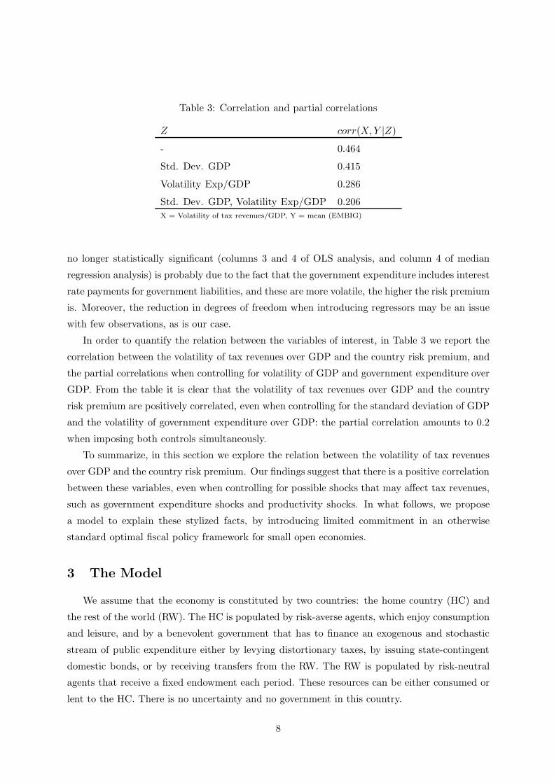
Table 3: Correlation and partial correlations

Z corr(X,Y |Z)

- 0.464

Std. Dev. GDP 0.415

Volatility Exp/GDP 0.286

Std. Dev. GDP, Volatility Exp/GDP 0.206

X = Volatility of tax revenues/GDP, Y = mean (EMBIG)

no longer statistically significant (columns 3 and 4 of OLS analysis, and column 4 of median

regression analysis) is probably due to the fact that the government expenditure includes interest

rate payments for government liabilities, and these are more volatile, the higher the risk premium

is. Moreover, the reduction in degrees of freedom when introducing regressors may be an issue

with few observations, as is our case.

In order to quantify the relation between the variables of interest, in Table 3 we report the

correlation between the volatility of tax revenues over GDP and the country risk premium, and

the partial correlations when controlling for volatility of GDP and government expenditure over

GDP. From the table it is clear that the volatility of tax revenues over GDP and the country

risk premium are positively correlated, even when controlling for the standard deviation of GDP

and the volatility of government expenditure over GDP: the partial correlation amounts to 0.2

when imposing both controls simultaneously.

To summarize, in this section we explore the relation between the volatility of tax revenues

over GDP and the country risk premium. Our findings suggest that there is a positive correlation

between these variables, even when controlling for possible shocks that may affect tax revenues,

such as government expenditure shocks and productivity shocks. In what follows, we propose

a model to explain these stylized facts, by introducing limited commitment in an otherwise

standard optimal fiscal policy framework for small open economies.

3 The Model

We assume that the economy is constituted by two countries: the home country (HC) and

the rest of the world (RW). The HC is populated by risk-averse agents, which enjoy consumption

and leisure, and by a benevolent government that has to finance an exogenous and stochastic

stream of public expenditure either by levying distortionary taxes, by issuing state-contingent

domestic bonds, or by receiving transfers from the RW. The RW is populated by risk-neutral

agents that receive a fixed endowment each period. These resources can be either consumed or

lent to the HC. There is no uncertainty and no government in this country.

8

3.1 The contract

The government of the HC can engage itself in a risk-sharing contract with the RW by

contracting transfers8. Let Tt be the amount of transfers received by the HC at time t. There

are three conditions that have to be met by {Tt}∞t=0.

First, the expected present discounted value of transfers exchanged with the RW must equal

zero:

E0

∞∑

t=0

βtTt = 0 (1)

where β is the discount factor of households in the RW and the HC. If both the HC and

the RW have full commitment, in the sense that they can commit to honor the contract in any

state of nature, this condition rules out net redistribution of wealth between countries. We call

this condition the fairness condition, since it implies that, given full commitment, ex-ante the

contract is fair from an actuarial point of view9.

If we assumed that the two parties in the contract have full commitment to pay back the debt

contracted with each other, equation (1) would be the only condition regulating international

flows. The allocations compatible with this situation will be our benchmark for comparison

purposes. However, when the government in the HC does not have a commitment technology, it

may decide to leave the contract if it finds it profitable to do so. Denote by V at the value of the

government’s outside option, i.e., the expected life-time utility of households in the HC if the

government leaves the contract, and by Vt the continuation value associated to staying in the

contract in any given period t. Then, in order to rule out default in equilibrium, the following

condition has to be satisfied

Vt ≡ Et

∞∑

j=0

βju(ct+j , lt+j) ≥ V at ∀t (2)

This condition constitutes a participation constraint for the HC. Notice that this participation

constraint may bind only in “good times”, i.e. for a low government expenditure shock. The

reason for this is that, when a good shock hits the economy, the value of the outside option

increases. In other words, in good times there is less need to resort to international risk sharing,

so the continuation value of the contract decreases relative to the outside (autarky) option. This

implies that the HC would want to default in good times. Although most theoretical models that

8In section 7 we show that these transfers can be reinterpreted as bonds traded in the international capitalmarket.

9This condition implies that the contract is actuarially fair only if the RW has full commitment. This is dueto the fact that, if the RW has limited commitment, the risk-free interest rate will not always be 1/β (see Section7 for further details). This condition is useful because it allows us to pin down the allocations. However, one canimpose other similar conditions that will yield different allocations.

9

incorporate default consider that this happens in bad times, Tomz and Wright (2007) provide

evidence showing that a significant fraction of defaults have occurred in good times.

We assume that if the government chooses to leave the contract at any given period, it re-

mains in autarky from that moment on. Moreover, when the government defaults on its external

obligations, it also defaults on its outstanding domestic debt. Consequently, the government is

forced to run a balanced budget thereafter10. Alternative assumptions to identify the costs of

default could be made, for example that, in case of default, the government cannot use external

funds, but it still has access to the domestic bonds market to smooth the distortions caused by

the expenditure shock. We have chosen the current specification for two reasons. First, this

allows us to keep the problem tractable, both from an analytical and a numerical point of view.

Second, this specification is consistent with the interpretation that the government is subject to

debt limits, as shown in Section 7.

Similar to the case of the HC, we assume that the RW also lacks a commitment technology

and can potentially exit the contract at any point in time. Therefore, we need to impose a

participation constraint for the RW :

Et

∞∑

j=0

βjTt+j ≤ B ∀t (3)

This condition is analogous to (2) and states that, at each point in time and for any contin-

gency, the expected discounted value of future transfers the HC is going to receive cannot exceed

an exogenous threshold value B. Notice that this constraint may bind only in bad times, i.e.,

for high government expenditure shocks, when the HC should receive transfers from the RW to

absorb the negative shock.

This restriction is meant to capture the fact that, for emerging economies, a sovereign debt

contract can cease not only because the country defaults, but also because the international

lender decides to stop lending money to the country. This may be due to contagion (in the

case of international crises), uncertainty about the fundamentals of the emerging economy, fear

of moral hazard issues, or simply because the lender cannot or does not want to transfer large

sums of money to the HC.

We use condition (3) because it is the natural counterpart of equation (2), and the introduc-

tion of these two constraints links our work to the existing literature on limited commitment11.

One can, of course, think of alternative constraints that may fulfill a similar task as (3). One

example is the constraint that we analyze in Appendix A.6 which imposes that the transfer Tt

10It follows that the only state variable influencing the outside option is the government expenditure shock.Therefore V a

t = V at (gt).

11Abraham and Carceles-Poveda (2006), Abraham and Carceles-Poveda (2009), Alvarez and Jermann (2000),Marcet and Marimon (1992),Kehoe and Perri (2002) and Scholl (2009) are some of the papers that study differentimplications of introducing limited commitment in a similar fashion as we do.

10

at a given time t cannot exceed a threshold B′. Given a proper calibration of the thresholds B

and B′, the qualitative implications of the model when using one constraint or the other remain

unchanged.

As long as conditions (1), (2) and (3) are satisfied, the government of the HC can choose

any given sequence {Tt}∞t=0 to partially absorb its expenditure shocks. Given constraint (1) and

the outside options V at and B, this contract is the one that maximizes risk-sharing among the

HC and the RW.

3.2 Households in the HC

Households in the HC derive utility from consumption and leisure, and each period are

endowed with one unit of time. The production function is linear in labor and one unit of labor

produces one unit of the consumption good. Therefore, wages wt = 1 ∀t. Households can save

or borrow by trading one-period contingent liabilities with the government.

The representative agent in the HC maximizes her expected lifetime utility

E0

∞∑

t=0

βtu(ct, lt)

subject to the period-by-period budget constraint

bt−1(gt) + (1 − τt)(1 − lt) = ct +∑

gt+1|gt

bt(gt+1)pbt(gt+1) (4)

where ct is private consumption, lt is leisure, bt(gt+1) denotes the amount of bonds issued

at time t contingent on the government expenditure shock in period t + 1, τt is the flat tax

rate on labor earnings and pbt(gt+1) is the price of a bond contingent on the expenditure shock

realization in the next period.

The optimality condition with respect to the state-contingent bond is:

pbt(gt+1) = βuc,t+1(g

t+1)

uc,tπ(gt+1|gt) (5)

.

where π(gt+1|gt) is the conditional probability of the government expenditure shock. Com-

bining the optimality conditions with respect to consumption and leisure we obtain the intratem-

poral condition

1 − τt =ul,t

uc,t(6)

11

3.3 Government of the HC

The government finances its exogenous stream of public expenditure {gt}∞t=0 by levying a

distortionary tax on labor income, by trading one-period state-contingent bonds with domestic

consumers and by contracting transfers with the RW. The government’s budget constraint is

gt = τt(1 − lt) +∑

gt+1|gt

bt(gt+1)pbt(gt+1) − bt−1(gt) + Tt (7)

3.4 Equilibrium

We proceed to define a competitive equilibrium with transfers in this economy.

Definition 1. A competitive equilibrium with transfers is given by allocations {c, l}, a price

system {pb}, government policies {g, τ l, b} and transfers T such that12:

1. Given prices and government policies, allocations satisfy the household’s optimality condi-

tions (4), (5) and (6).

2. Given allocations and prices, government policies satisfy the sequence of government budget

constraints (7).

3. Given allocations, prices and government policies, transfers satisfy conditions (1), (2) and

(3).

4. Allocations satisfy the sequence of feasibility constraints:

ct + gt = 1 − lt + Tt (8)

3.5 Optimal policy

The government of the HC behaves as a benevolent Ramsey Planner and chooses tax rates,

bonds and transfers {ct, bt, Tt}∞t=0 in order to maximize the representative household’s life-time

expected utility, subject to the constraints imposed by the definition of competitive equilibrium.

Before studying the consequences of introducing limited commitment in terms of the optimal

fiscal plan, it is instructive to analyze the benchmark scenario in which both the government in

the HC and the RW have a full commitment technology.

12We follow the notation of Ljungqvist and Sargent (2000) and use symbols without subscripts to denote theone-sided infinite sequence for the corresponding variable, e.g., c ≡ {ct}

∞t=0.

12

3.5.1 Full commitment

If both the HC and the RW can commit to honor their external obligations in all states of

nature, conditions (2) and (3) need not be specified in the contract. Then, the problem of the

Ramsey planner is

max{ct,lt}

∞t=0

E0

∞∑

t=0

βtu(ct, lt)

s.t.

b−1uc,0 = E0

∞∑

t=0

βt(uc,tct − ul,t(1 − lt)) (9)

ct + gt = 1 − lt + Tt (10)

E0

∞∑

t=0

βtTt = 0 (11)

Equation (9) is the intertemporal budget constraint of households, after imposing the transver-

sality condition and plugging in the optimality conditions of the household’s problem (5) and

(6). This condition is known in the literature of optimal fiscal policy as the implementability

condition.

The optimality conditions for t ≥ 113 are:

uc,t + ∆(ucc,tct + uc,t + ucl,t(1 − lt)) = λ (12)

ul,t + ∆(ucl,tct + ul,t − ull,t(1 − lt)) = λ (13)

where λ is the multiplier associated with constraint (11), and ∆ is the multiplier associated

with the implementability condition (9). The next proposition characterizes the equilibrium.

Proposition 1. Under full commitment, consumption, labor and taxes are constant ∀t ≥ 1.

Moreover, if b−1 = 0, bt(gt+1) = 0 ∀t, ∀gt+1 and the government perfectly absorbs the public

expenditure shocks through transfers Tt.

Proof. Using optimality conditions (12) and (13) we have two equations to determine two un-

knowns, ct and lt, given the lagrange multipliers λ and ∆. Since these two equations are inde-

pendent of the current shock gt, the allocations are constant ∀t ≥ 1. From the intratemporal

optimality condition of households (6) it can be seen that the tax rate τ lt is also constant ∀t ≥ 1.

13Notice that if b−1 6= 0 the Ramsey problem is not recursive for t ≥ 0. This constitutes the standard source oftime inconsistency in these type of optimal policy problem. However, the problem becomes recursive for t ≥ 1. Inthe numerical exercises that follow we solve the problem taking into account that optimality conditions for t = 0are different from the rest.

13

Finally, when b−1 = 0 the intertemporal budget constraint of households at time t = 0 (equation

(9)) can be written as

1

1 − β(ucc− ul(1 − l)) = 0

Notice that, for any given time t+ 1, domestic bond holdings bt(gt+1) are obtained from the

intertemporal budget constraint of households in that period, i.e.,

bt(gt+1)uc,t+1 = Et+1

∞∑

j=0

βj(uc,t+1+jct+1+j − ul,t+1+j(1 − lt+1+j))

However, since the allocations are constant over time, it is the case that

bt(gt+1)uc = Et+1

∞∑

j=0

βj(ucc− ul(1 − l)) =1

1 − β(ucc− ul(1 − l)) = 0

Therefore, bt(gt+1) = 0 ∀gt+1 and, from the feasibility constraint (10), it follows that all

fluctuations in gt must be absorbed by Tt.

Proposition 1 illustrates the effect of full risk-sharing on the optimal fiscal policy plan:

being consumption and leisure constant in time, the optimal tax rate is constant as well. The

government in the HC uses transfers from the RW to completely absorb the shock. When gt

is higher than average, the government uses transfers to finance its expenditure; conversely,

when gt is below average, the government uses the proceeds from taxation to pay back transfers

received in the past14. In this way, the RW provides full insurance to the domestic economy.

3.5.2 Limited Commitment

We consider the case in which neither the government in the HC nor the RW can commit to

repay external debt. The problem of the Ramsey planner is identical to the one in the previous

section, but now conditions (2) and (3) have to be explicitly taken into account:

max{ct,lt,Tt}

∞t=0

E0

∞∑

t=0

βtu(ct, lt)

subject to

ct + gt = (1 − lt) + Tt (14)

14In Appendix A.2 we study the case in which the utility function is logarithmic in its two arguments. In sucha case, it is easy to see that transfers behave exactly as described here.

14

E0

∞∑

t=0

βt(uc,tct − ul,t(1 − lt)) = uc1,0(b−1) (15)

E0

∞∑

t=0

βtTt = 0 (16)

Et

∞∑

j=0

βju(ct+j , lt+j) ≥ V a(gt)∀t (17)

Et

∞∑

j=0

βjTt+j ≤ B ∀t (18)

Since the participation constraint at time t (17) includes future endogenous variables that

influence the current allocation, standard dynamic programming results do not apply directly.

To overcome this problem we apply the approach described in Marcet and Marimon (2009) and

write the Lagrangian as:

L = E0

∞∑

t=0

βt[(1 + γ1t )u(ct, lt) − ψt(ct + gt − (1 − lt) − Tt)

− µ1t (V

at ) + µ2

t (B) − ∆(uc,tct − ul,t(1 − lt)) − Tt(λ+ γ2t )] + ∆(uc,0(b−1))

where

γ1t = γ1

t−1 + µ1t ; γ2

t = γ2t−1 + µ2

t

for γ1−1 = 0 and γ2

−1 = 0. ∆ is the Lagrange multiplier associated to equation (15), ψt is

the Lagrange multiplier associated to equation (14), λ is the Lagrange multiplier associated to

equation (16), µ1t is the Lagrange multiplier associated to equation (17) and µ2

t is the Lagrange

multiplier associated to equation (18). γ1t and γ2

t are the sum of past Lagrange multipliers µ1 and

µ2 respectively, and summarize all the past periods in which either constraint has been binding.

Intuitively, γ1 and γ2 can be thought of as the collection of past compensations promised to

each country so that it would not have incentives to leave the contract15.

It can be shown that, for t ≥ 116, the solution to the problem stated above is given by

time-invariant policy functions that depend on the augmented state space G × Γ1 × Γ2, where

G = {g1, g2, . . . , gn} is the set of all possible realizations of the public expenditure shock gt and

Γ1 and Γ2 are the sets of all possible realizations of the costate variables γ1 and γ2, respectively.

15Strictly speaking, it can be the case that a participation constraint is binding, and yet its associated Lagrangemultiplier is zero. However, in this case, the fact that the participation constraint binds would not alter theallocations and, consequently, there would not be a change in γ.

16Once again, for t = 0 the optimality conditions of the problem are different. Applying Marcet and Marimon(2009), the problem only becomes recursive from t ≥ 1 onwards.

15

Therefore,

ct

lt

Tt

µ1t

µ2t

= H(gt, γ1t−1, γ

2t−1) ∀t ≥ 1

More specifically, the government’s optimality conditions for t ≥ 1 are:

uc,t(1 + γ1t ) − ψt − ∆(ucc,tct + uc,t − ucl,t(1 − lt)) = 0 (19)

ul,t(1 + γ1t ) − ψt − ∆(ucl,tct + ul,t − ull,t(1 − lt)) = 0 (20)

ψt = λ+ γ2t (21)

Other optimality conditions are equations (14) to (18) and:

µ1t (Et

∞∑

j=0

βju(ct+j , lt+j) − V a(gt)) = 0 (22)

µ2t (Et

∞∑

j=0

βjTt+j −B) = 0 (23)

γ1t = µ1

t + γ1t−1; µ1

t ≥ 0 (24)

γ2t = µ2

t + γ2t−1; µ2

t ≥ 0 (25)

From (19), (20) and (21) it is immediate to see that now the presence of γ1t−1 and γ2

t−1 makes

the allocations state-dependent. Moreover, being γ1t−1 and γ2

t−1 functions of all the past shocks

hitting the economy, the allocations are actually history-dependent.

Notice also that the presence of these Lagrange multipliers makes the cost of distortionary

taxation state-dependent. While in the full-commitment case this cost is constant over time and

across states, in the limited commitment case it changes depending on the incentives to default

that the HC and the RW have17. We will discuss this is further detail in Section 7.

The next proposition characterizes the equilibrium for a logarithmic utility function.

Proposition 2. Consider a utility function logarithmic in consumption and leisure and separable

in the two arguments:

17It can be shown that, in the full commitment case, this cost is given by ∆, while in the limited commitmentone is determined by ∆

1+γ1

t

.

16

u(ct, lt) = αlog(ct) + δlog(lt) (26)

with α > 0 and δ > 0. Define t < t′:

1. If the participation constraint (17) binds such that γ1t < γ1

t′ , then ct < ct′ , lt < lt′ and

τt > τt′ .

2. If the participation constraint (18) binds such that γ2t < γ2

t′ , then ct > ct′ , lt > lt′ and

τt < τt′ .

Proof. See Appendix A.3.

Proposition 2 states the way the allocations and tax rates adjust in order to make the contract

incentive-compatible for the HC and the RW. As long as neither participation constraint binds,

consumption and leisure remain constant.

In order to gain intuition, consider the case in which, at period t′, the participation constraint

of the HC (equation (17)) is not satisfied when µ1t′ = 0. Then, as the HC has incentives to go into

autarky, the contract has to be such that the expected lifetime utility of households of the HC

increases so as to make (17) hold with equality. For this to be the case, µ1t′ > 0, and consequently

ct′ and lt′ jump upwards. Moreover, because the utility function is strictly concave, it is efficient

to increase consumption and leisure permanently through a higher γ1t′ , rather than to increase

them substantially for only one period. The increase in utility also dictates a decrease in tax

rates so as to increase the net income of households. The intuition for the case in which the

participation constraint (18) of the RW binds is exactly analogous to the previous one.

The fact that the tax rates now depend on γ1t and γ2

t implies that, if equations (17) and

(18) are effectively binding at certain periods, tax rates are more volatile than under the full

commitment scenario.

4 An example of labor tax-smoothing

To understand better the impact of limited commitment on the ability of the government to

smooth taxes, in this section we analyze the case study of a perfectly anticipated government

expenditure shock. The example follows closely one of the examples of tax smoothing in Lucas

and Stokey (1983).

Suppose that government expenditure is known to be constant and equal to 0 in all periods

except in T , when gT > 0. In order to simplify the analysis, throughout this section we assume

that B is large so that the RW never has incentives to leave the contract. Moreover, we assume

that b−1 = 0 and that households have a logarithmic utility function as (26).

17

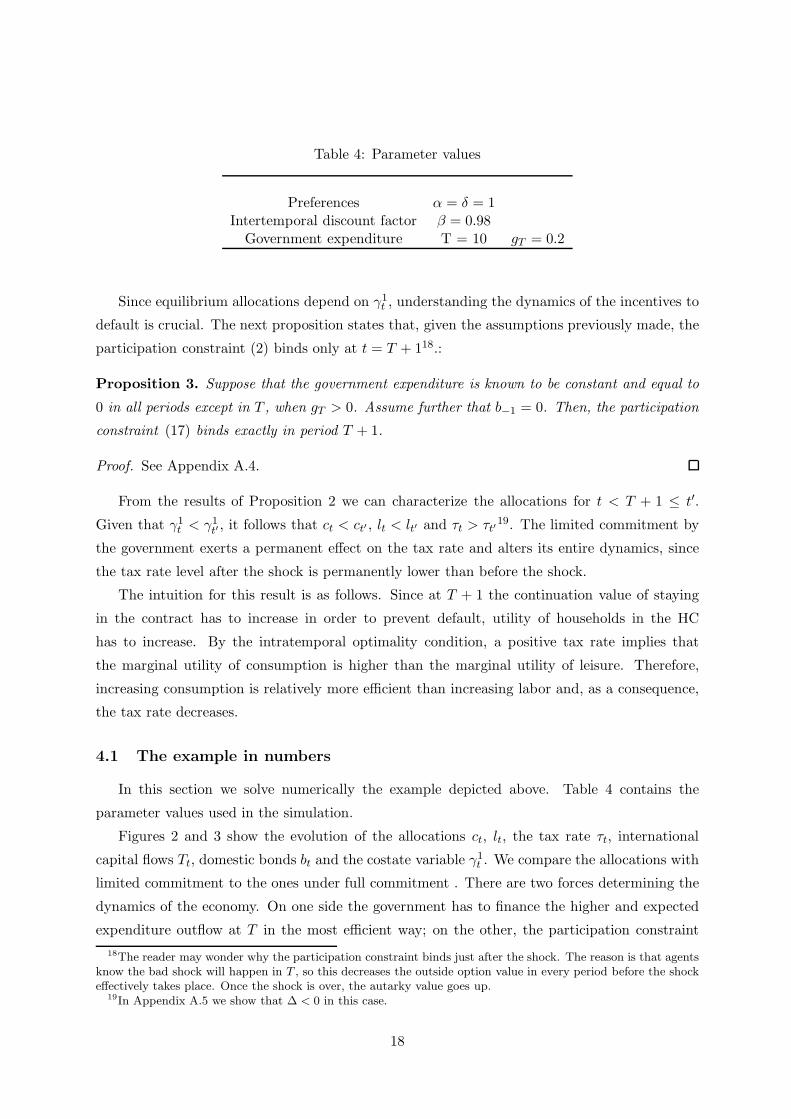
Table 4: Parameter values

Preferences α = δ = 1Intertemporal discount factor β = 0.98

Government expenditure T = 10 gT = 0.2

Since equilibrium allocations depend on γ1t , understanding the dynamics of the incentives to

default is crucial. The next proposition states that, given the assumptions previously made, the

participation constraint (2) binds only at t = T + 118.:

Proposition 3. Suppose that the government expenditure is known to be constant and equal to

0 in all periods except in T , when gT > 0. Assume further that b−1 = 0. Then, the participation

constraint (17) binds exactly in period T + 1.

Proof. See Appendix A.4.

From the results of Proposition 2 we can characterize the allocations for t < T + 1 ≤ t′.

Given that γ1t < γ1

t′ , it follows that ct < ct′ , lt < lt′ and τt > τt′19. The limited commitment by

the government exerts a permanent effect on the tax rate and alters its entire dynamics, since

the tax rate level after the shock is permanently lower than before the shock.

The intuition for this result is as follows. Since at T + 1 the continuation value of staying

in the contract has to increase in order to prevent default, utility of households in the HC

has to increase. By the intratemporal optimality condition, a positive tax rate implies that

the marginal utility of consumption is higher than the marginal utility of leisure. Therefore,

increasing consumption is relatively more efficient than increasing labor and, as a consequence,

the tax rate decreases.

4.1 The example in numbers

In this section we solve numerically the example depicted above. Table 4 contains the

parameter values used in the simulation.

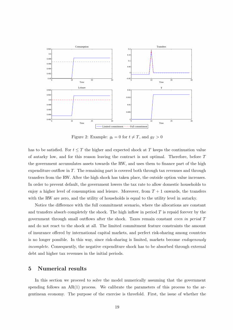
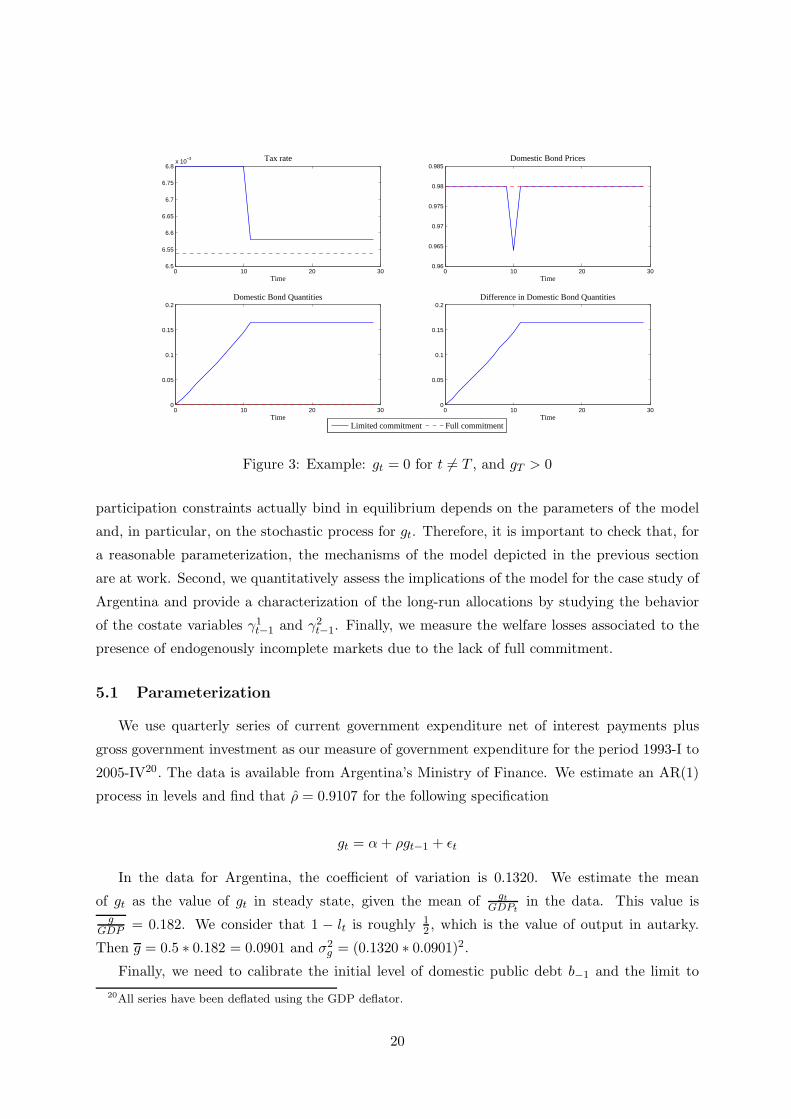
Figures 2 and 3 show the evolution of the allocations ct, lt, the tax rate τt, international

capital flows Tt, domestic bonds bt and the costate variable γ1t . We compare the allocations with

limited commitment to the ones under full commitment . There are two forces determining the

dynamics of the economy. On one side the government has to finance the higher and expected

expenditure outflow at T in the most efficient way; on the other, the participation constraint

18The reader may wonder why the participation constraint binds just after the shock. The reason is that agentsknow the bad shock will happen in T , so this decreases the outside option value in every period before the shockeffectively takes place. Once the shock is over, the autarky value goes up.

19In Appendix A.5 we show that ∆ < 0 in this case.

18

0 10 20 300.49

0.492

0.494

0.496

0.498

0.5

0.502

Time

Consumption

0 10 20 30−0.05

0

0.05

0.1

0.15

0.2

Time

Transfers

0 10 20 300.492

0.494

0.496

0.498

0.5

0.502

0.504

Time

Leisure

Limited commitment Full commitment

0 10 20 300

0.005

0.01

0.015

0.02

Time

γ

Figure 2: Example: gt = 0 for t 6= T , and gT > 0

has to be satisfied. For t ≤ T the higher and expected shock at T keeps the continuation value

of autarky low, and for this reason leaving the contract is not optimal. Therefore, before T

the government accumulates assets towards the RW, and uses them to finance part of the high

expenditure outflow in T . The remaining part is covered both through tax revenues and through

transfers from the RW. After the high shock has taken place, the outside option value increases.

In order to prevent default, the government lowers the tax rate to allow domestic households to

enjoy a higher level of consumption and leisure. Moreover, from T + 1 onwards, the transfers

with the RW are zero, and the utility of households is equal to the utility level in autarky.

Notice the difference with the full commitment scenario, where the allocations are constant

and transfers absorb completely the shock. The high inflow in period T is repaid forever by the

government through small outflows after the shock. Taxes remain constant even in period T

and do not react to the shock at all. The limited commitment feature constraints the amount

of insurance offered by international capital markets, and perfect risk-sharing among countries

is no longer possible. In this way, since risk-sharing is limited, markets become endogenously

incomplete. Consequently, the negative expenditure shock has to be absorbed through external

debt and higher tax revenues in the initial periods.

5 Numerical results

In this section we proceed to solve the model numerically assuming that the government

spending follows an AR(1) process. We calibrate the parameters of this process to the ar-

gentinean economy. The purpose of the exercise is threefold. First, the issue of whether the

19

0 10 20 306.5

6.55

6.6

6.65

6.7

6.75

6.8x 10

−3

Time

Tax rate

0 10 20 300.96

0.965

0.97

0.975

0.98

0.985

Time

Domestic Bond Prices

0 10 20 300

0.05

0.1

0.15

0.2

Time

Domestic Bond Quantities

Limited commitment Full commitment

0 10 20 300

0.05

0.1

0.15

0.2

Time

Difference in Domestic Bond Quantities

Figure 3: Example: gt = 0 for t 6= T , and gT > 0

participation constraints actually bind in equilibrium depends on the parameters of the model

and, in particular, on the stochastic process for gt. Therefore, it is important to check that, for

a reasonable parameterization, the mechanisms of the model depicted in the previous section

are at work. Second, we quantitatively assess the implications of the model for the case study of

Argentina and provide a characterization of the long-run allocations by studying the behavior

of the costate variables γ1t−1 and γ2

t−1. Finally, we measure the welfare losses associated to the

presence of endogenously incomplete markets due to the lack of full commitment.

5.1 Parameterization

We use quarterly series of current government expenditure net of interest payments plus

gross government investment as our measure of government expenditure for the period 1993-I to

2005-IV20. The data is available from Argentina’s Ministry of Finance. We estimate an AR(1)

process in levels and find that ρ = 0.9107 for the following specification

gt = α+ ρgt−1 + ǫt

In the data for Argentina, the coefficient of variation is 0.1320. We estimate the mean

of gt as the value of gt in steady state, given the mean of gt

GDPtin the data. This value is

gGDP

= 0.182. We consider that 1 − lt is roughly 12 , which is the value of output in autarky.

Then g = 0.5 ∗ 0.182 = 0.0901 and σ2g = (0.1320 ∗ 0.0901)2.

Finally, we need to calibrate the initial level of domestic public debt b−1 and the limit to

20All series have been deflated using the GDP deflator.

20

Table 5: Parameter values

Preferences α = δ = 1Intertemporal discount factor β = 0.98

Government expenditure process gt = α+ ρgt−1 + ǫtg∗ 0.1820 ∗ 0.5ρg 0.9107σ2g 0.1320 ∗ 0.091

B 0.0402b−1 0.034

transfers from the rest of the world, B. To compute a value for the first concept, we need to

consider public debt held by nationals. Since we do not have data on debt ownership, we consider

debt issued in national currency as a proxy for debt held by nationals. We do not have data

on debt issued in national currency before the fourth quarter of 1993, so we compute the mean

percentage of public debt issued in national currency for the period IV-1993 to IV-2004, which

is about 10%21. Then, we multiply the total public debt of the first quarter of 1993 divided

by annual GDP by this percentage and multiply it by approximate annual GDP of the model:

0.17 ∗ 0.1 ∗ 2 = 0.034.

The calibration of B is more cumbersome. First, notice that Tt can be interpreted as the

change in public debt contracted with foreign creditors in a given period. We will use debt

contracted with the IMF, so that Tt = bIMFt − bIMF

t−1 , where bIMFt is debt over annualized GDP

from the data, multiplied by the approximate annual GDP of the model. Then B is computed

from the data in the following manner:

B = EI−93

∞∑

j=0

βj Tt+j (27)

where Tt is the simulated change in debt with the IMF in a given period. To simulate

the series {Tt+j}∞j=0 we estimate an AR(1) process for bIMF

t+j from the data and construct Tt,

according to the definition of transfers previously specified. Finally, we compute the expectation

in (27) as the mean of 10000 replications of discounted sums of transfers, of 1000 periods each,

where the initial level of debt bIMFt = bIMF

I−93 is taken from the data22.

21We do not consider data for the year 2005 because during that period, as part of the debt renegotiation afterthe sovereign default of 2001, a large fraction of public debt originally issued in US dollars was re-denominatedin argentinean pesos.

22We only consider data until the year 2000 because, during 2001 and specially in the months prior to thesovereign default of 2001, the debt contracted with the IMF grew from 3278 million US dollars (III-2000) to 14592million US dollars (III-2001). This large increase in the debt contracted with the IMF is due to the profoundeconomic and political crisis that the country went through during that period, and does not reflect the normalevolution of debt in the previous more stable years.

21

0 20 40 60 80 100 120 140 160 180 2000.39

0.395

0.4

0.405

0.41

0.415

0.42

0.425

Time

Consumption

0 20 40 60 80 100 120 140 160 180 200−0.03

−0.02

−0.01

0

0.01

0.02

0.03

Time

Transfers to HC

0 20 40 60 80 100 120 140 160 180 2000.49

0.495

0.5

0.505

0.51

0.515

Time

Leisure

Limited commitmentFull commitment

Figure 4: Allocations

5.2 Results

Figures 4, 5 and 6 show the allocations, co-state variables and fiscal variables respectively

for a particular realization of the government expenditure shock, for the case in which the

government of the HC and the RW have limited commitment (solid line). For comparison

purposes, we show the same variables under full commitment (dashed line). Appendix A.9

explains the computational algorithm used to solve the model23.

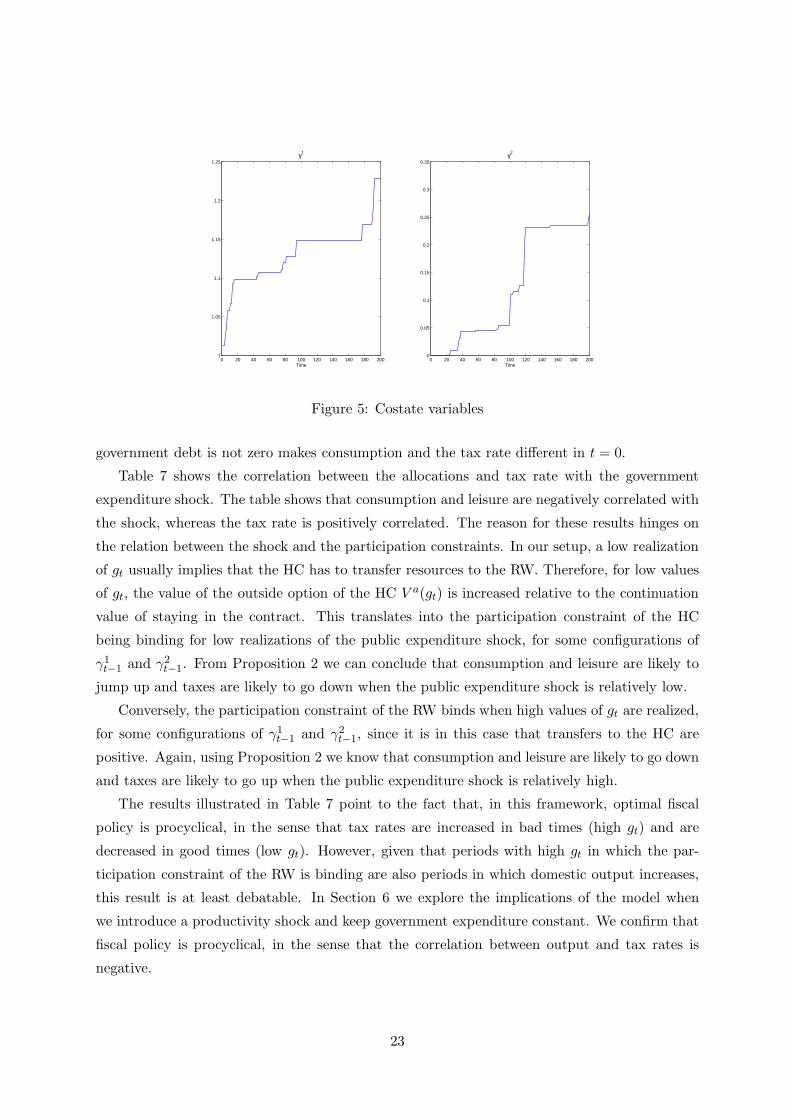
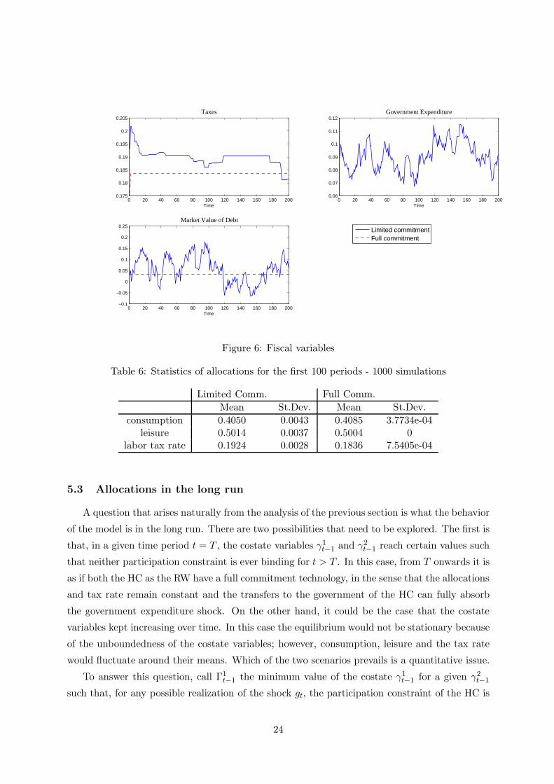
We can observe from Figure 5 that both participation constraints bind often for this partic-

ular realization of the shock. This causes the allocations to jump upwards and downwards, and

consequently to be more volatile than in the benchmark case of full commitment. It is clear from

Figure 6 that the tax rate is also more volatile than in the full commitment case. Moreover, in

the limited commitment case the government of the HC makes active use of the domestic bond

market to improve its ability to smooth taxes.

Tables 6 and 7 show some statistics obtained by simulating the model for 1000 realizations of

the shock of 100 periods each24. Notice first that, while the average values of the allocations are

roughly the same with limited commitment as with full commitment, their standard deviation

is much higher in the first case. In the full commitment case, if b−1 = 0, consumption, leisure

and the tax rate would be constant from period 0. The fact that the initial stock of domestic

23We only show the first 200 periods of the simulation because, for this simulation and this time span, thecostate variables remain within the grid for which the model has been solved.

24Once more, we consider only the first 100 periods in order to make sure that the costate variables do not exitthe grid used to solve the model.

22

0 20 40 60 80 100 120 140 160 180 2001

1.05

1.1

1.15

1.2

1.25

Time

γ1

0 20 40 60 80 100 120 140 160 180 2000

0.05

0.1

0.15

0.2

0.25

0.3

0.35

Time

γ2

Figure 5: Costate variables

government debt is not zero makes consumption and the tax rate different in t = 0.

Table 7 shows the correlation between the allocations and tax rate with the government

expenditure shock. The table shows that consumption and leisure are negatively correlated with

the shock, whereas the tax rate is positively correlated. The reason for these results hinges on

the relation between the shock and the participation constraints. In our setup, a low realization

of gt usually implies that the HC has to transfer resources to the RW. Therefore, for low values

of gt, the value of the outside option of the HC V a(gt) is increased relative to the continuation

value of staying in the contract. This translates into the participation constraint of the HC

being binding for low realizations of the public expenditure shock, for some configurations of

γ1t−1 and γ2

t−1. From Proposition 2 we can conclude that consumption and leisure are likely to

jump up and taxes are likely to go down when the public expenditure shock is relatively low.

Conversely, the participation constraint of the RW binds when high values of gt are realized,

for some configurations of γ1t−1 and γ2

t−1, since it is in this case that transfers to the HC are

positive. Again, using Proposition 2 we know that consumption and leisure are likely to go down

and taxes are likely to go up when the public expenditure shock is relatively high.

The results illustrated in Table 7 point to the fact that, in this framework, optimal fiscal

policy is procyclical, in the sense that tax rates are increased in bad times (high gt) and are

decreased in good times (low gt). However, given that periods with high gt in which the par-

ticipation constraint of the RW is binding are also periods in which domestic output increases,

this result is at least debatable. In Section 6 we explore the implications of the model when

we introduce a productivity shock and keep government expenditure constant. We confirm that

fiscal policy is procyclical, in the sense that the correlation between output and tax rates is

negative.

23

0 20 40 60 80 100 120 140 160 180 2000.175

0.18

0.185

0.19

0.195

0.2

0.205

Time

Taxes

0 20 40 60 80 100 120 140 160 180 2000.06

0.07

0.08

0.09

0.1

0.11

0.12

Time

Government Expenditure

0 20 40 60 80 100 120 140 160 180 200−0.1

−0.05

0

0.05

0.1

0.15

0.2

0.25

Time

Market Value of Debt

Limited commitmentFull commitment

Figure 6: Fiscal variables

Table 6: Statistics of allocations for the first 100 periods - 1000 simulations

Limited Comm. Full Comm.

Mean St.Dev. Mean St.Dev.

consumption 0.4050 0.0043 0.4085 3.7734e-04leisure 0.5014 0.0037 0.5004 0

labor tax rate 0.1924 0.0028 0.1836 7.5405e-04

5.3 Allocations in the long run

A question that arises naturally from the analysis of the previous section is what the behavior

of the model is in the long run. There are two possibilities that need to be explored. The first is

that, in a given time period t = T , the costate variables γ1t−1 and γ2

t−1 reach certain values such

that neither participation constraint is ever binding for t > T . In this case, from T onwards it is

as if both the HC as the RW have a full commitment technology, in the sense that the allocations

and tax rate remain constant and the transfers to the government of the HC can fully absorb

the government expenditure shock. On the other hand, it could be the case that the costate

variables kept increasing over time. In this case the equilibrium would not be stationary because

of the unboundedness of the costate variables; however, consumption, leisure and the tax rate

would fluctuate around their means. Which of the two scenarios prevails is a quantitative issue.

To answer this question, call Γ1t−1 the minimum value of the costate γ1

t−1 for a given γ2t−1

such that, for any possible realization of the shock gt, the participation constraint of the HC is

24

Table 7: Correlation with shock

Limited Comm. Full Comm.

Corr(x, g) Corr(x, g)

consumption -0.5765 0.0001leisure -0.7071 0

labor tax rate 0.2881 -0.0001

1 1.05 1.1 1.15 1.2 1.25 1.3 1.350

0.1

0.2

0.3

0.4

0.5

0.6

0.7

0.8

0.9

γ1t−1

γ2 t−1

Γ2t−1

Γ1t−1

Figure 7: Long-run analysis

satisfied. Define Γ2t−1 in a similar fashion. Then,

argminΓ1t−1

W (gt,Γ1t−1, γ

2t−1) = Et

∞∑

j=0

βju(ct+j , lt+j) ≥ V at (gt) ∀gt ∈ {gmin, g

max}

argminΓ2t−1

W (gt, γ1t−1,Γ

2t−1) = Et

∞∑

j=0

βjTt+j ≤ B ∀gt ∈ {gmin, gmax}

Figure 7 shows the computed Γ1t−1 and Γ2

t−1 for our previous parameterization25. Notice

that, for any configuration of γ1t−1 and γ2

t−1 that lies in the region to the right of the solid line,

the participation constraint of the HC is never binding. Similarly, for any configuration of γ1t−1

and γ2t−1 that lies in the region above the dashed line, the participation constraint of the RW is

never binding.

The fact that both lines cross implies that the multipliers will increase until a given time

period t = T , in which the Γ1t−1 and the Γ2

t−1 lines meet. At that point, the costate variables

have reached the area in which the participation constraints are never binding again and the

25For the computation, we extend the original grid for γ1t−1 and γ2

t−1 to characterize the behavior of the costatevariables on a larger set. Although this implies a reduction in precision, in this subsection we are only interestedin the characterization of the long run, and not in the precision of the simulations.

25

equilibrium is stationary. In particular, for t ≥ T consumption, leisure and the tax rate are

constant, and lifetime expected discounted utility of households when the HC stays in the

contract is equal to the highest possible value of the outside option, which will correspond to

the value of autarky when the government expenditure shock is the lowest possible.

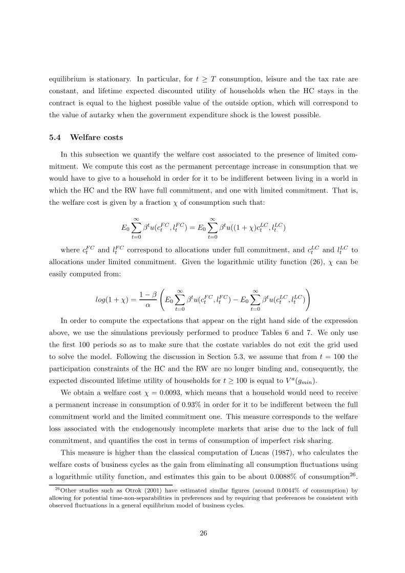
5.4 Welfare costs

In this subsection we quantify the welfare cost associated to the presence of limited com-

mitment. We compute this cost as the permanent percentage increase in consumption that we

would have to give to a household in order for it to be indifferent between living in a world in

which the HC and the RW have full commitment, and one with limited commitment. That is,

the welfare cost is given by a fraction χ of consumption such that:

E0

∞∑

t=0

βtu(cFCt , lFCt ) = E0

∞∑

t=0

βtu((1 + χ)cLCt , lLCt )

where cFCt and lFCt correspond to allocations under full commitment, and cLCt and lLCt to

allocations under limited commitment. Given the logarithmic utility function (26), χ can be

easily computed from:

log(1 + χ) =1 − β

α

(

E0

∞∑

t=0

βtu(cFCt , lFCt ) −E0

∞∑

t=0

βtu(cLCt , lLCt )

)

In order to compute the expectations that appear on the right hand side of the expression

above, we use the simulations previously performed to produce Tables 6 and 7. We only use

the first 100 periods so as to make sure that the costate variables do not exit the grid used

to solve the model. Following the discussion in Section 5.3, we assume that from t = 100 the

participation constraints of the HC and the RW are no longer binding and, consequently, the

expected discounted lifetime utility of households for t ≥ 100 is equal to V a(gmin).

We obtain a welfare cost χ = 0.0093, which means that a household would need to receive

a permanent increase in consumption of 0.93% in order for it to be indifferent between the full

commitment world and the limited commitment one. This measure corresponds to the welfare

loss associated with the endogenously incomplete markets that arise due to the lack of full

commitment, and quantifies the cost in terms of consumption of imperfect risk sharing.

This measure is higher than the classical computation of Lucas (1987), who calculates the

welfare costs of business cycles as the gain from eliminating all consumption fluctuations using

a logarithmic utility function, and estimates this gain to be about 0.0088% of consumption26.

26Other studies such as Otrok (2001) have estimated similar figures (around 0.0044% of consumption) byallowing for potential time-non-separabilities in preferences and by requiring that preferences be consistent withobserved fluctuations in a general equilibrium model of business cycles.

26

However, our measure is in line with Aiyagari et al. (2002), who compute the welfare costs of

incomplete markets in a model of optimal taxation without state-contingent debt and find this

cost to be as high as 0.96% in one of their examples.

6 Procyclicality of fiscal policy

In the recent past there has been a significant interest in studying the cyclical properties of

fiscal policy in emerging countries, both from an empirical as well as a theoretical perspective.

For this reason, in this section we assess whether our model generates procyclical or counter-

cyclical fiscal policy. By procyclical fiscal policy, we understand higher public expenditure and

lower tax rates in good times, when GDP is relatively high, and lower public expenditure and

higher tax rates in bad times, when GDP is relatively low.

6.1 Evidence and some theory

A number of authors have documented the fact that fiscal policy appears to be procyclical

in emerging economies, whereas it is countercyclical or acyclical in developed economies27. One

of the earliest contributions is Gavin and Perotti (1997), who find evidence of procyclical fiscal

policy for 13 Latinamerican economies. Using a sample of 56 countries, Talvi and Vegh (2005)

find that the correlation between government consumption and output in the G-7 countries is

close to zero. However, for emerging economies this correlation is significantly positive. In

a similar vein, Kaminsky et al. (2004) document, based on a sample of 104 countries, that

government spending increases in good times and falls in bad times for the majority of emerging

countries in their sample. More recently, Ilzetzki and Vegh (2008) build a quarterly data set for 49

countries covering the period 1960-2006 and, in order to tackle issues of endogeneity, they subject

the data to a battery of econometric tests such as instrumental variables, simultaneous equations,

and time-series methods. The authors find strong evidence that fiscal policy is procyclical in

emerging economies, while it is acyclical in high-income countries.

Despite the broad literature cited above, there is little evidence on the cyclical properties of

tax rates. The main reason for this is data availability: while data on government consumption is

fairly easy to obtain, data on tax rates is very scarce. Mendoza et al. (1994) compute time series

of effective tax rates on consumption, capital income and labor income for G-7 countries using

data on tax revenues and national accounts. Unfortunately, these series are hard to construct

in the case of emerging economies, as usually the information on revenues is not disaggregated

enough. However, as Cuadra et al. (2010) point out, several episodes suggest that in emerging

27For a careful review of the literature on cyclicality of fiscal policy in emerging economies, see Cuadra et al.(2010).

27

countries tax rates behave according to a procyclical fiscal policy plan28.

This evidence for emerging countries is at odds with what the classical literature on optimal

fiscal policy dictates. Neoclassical models in the spirit of Barro (1979) and Lucas and Stokey

(1983) prescribe that fiscal policy should remain neutral over the business cycle. On the other

hand, keynesian models suggest that fiscal policy should be countercyclical, in the belief that

the fiscal multipliers are significantly positive (and larger than 1). More recently, there has been

a renewed interest in rationalizing the conventional wisdom that countercyclical fiscal policy can

have a stabilizing role in the economy. In this vein, Christiano et al. (2009) show, in a New

Keynesian framework, that if the zero lower bound on the nominal interest rate is binding, the

government spending multiplier is large. This apparent puzzle has led many authors to seek

reasonable explanations that reconcile the theory with the empirical facts.

As Ilzetzki and Vegh (2008) point out, the literature has followed two main paths to explain

the phenomenon at hand. One set of papers is based on the notion that emerging economies

have imperfect access to financial markets that prevents them from borrowing in bad times.

Riascos and Vegh (2003) and Cuadra et al. (2010) develop models that rely on this idea29. The

intuition behind the mechanism that links this imperfect access to credit markets to procyclical

fiscal policy is simple: when the government has limited ability to issue debt during crises, it

will have to reduce public spending, increase tax rates, or a combination of both. Alternatively,

papers such as Lane and Tornell (1999), Talvi and Vegh (2005) and Alesina et al. (2008) exploit

political economy arguments based on the idea that good times encourage fiscal leniency and

rent-seeking activities.

6.2 Cyclical properties of fiscal policy in the presence of limited commitment

In Section 5.2 we have already argued that, when considering a government expenditure

shock, the model suggested that fiscal policy is procyclical, in the sense that tax rates are

increased in bad times and decreased in good ones. However, this conclusion is somehow blurred

by the fact that these results are obtained in a context in which the shock governing the cycle

is a fiscal expenditure shock.

In order to be able to clearly characterize the cyclical properties of fiscal policy in the presence

of limited commitment, in this section we keep government spending fixed and instead consider

that the source of fluctuations in the economy is a productivity shock. The production function

now is described by

yt = exp(zt)(1 − lt)

28See Cuadra et al. (2010) for a description of such episodes.29Gavin and Perotti (1997) stress the role of borrowing constraints in explaining the procyclicality of fiscal

policy in Latin America. However, they do not develop a formal model to rationalize the idea.

28

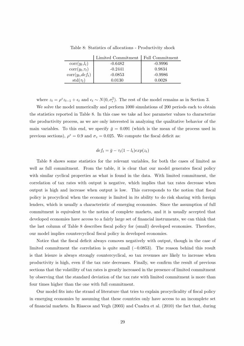
Table 8: Statistics of allocations - Productivity shock

Limited Commitment Full Commitment

corr(yt,lt) -0.6482 -0.9996corr(yt,τt) -0.2441 0.9834

corr(yt,deft) -0.0853 -0.9986std(τt) 0.0130 0.0028

where zt = ρzzt−1 + ǫt and ǫt ∼ N(0, σ2ǫ ). The rest of the model remains as in Section 3.

We solve the model numerically and perform 1000 simulations of 200 periods each to obtain

the statistics reported in Table 8. In this case we take ad hoc parameter values to characterize

the productivity process, as we are only interested in analyzing the qualitative behavior of the

main variables. To this end, we specify g = 0.091 (which is the mean of the process used in

previous sections), ρz = 0.9 and σz = 0.025. We compute the fiscal deficit as:

deft = g − τt(1 − lt)exp(zt)

Table 8 shows some statistics for the relevant variables, for both the cases of limited as

well as full commitment. From the table, it is clear that our model generates fiscal policy

with similar cyclical properties as what is found in the data. With limited commitment, the

correlation of tax rates with output is negative, which implies that tax rates decrease when

output is high and increase when output is low. This corresponds to the notion that fiscal

policy is procyclical when the economy is limited in its ability to do risk sharing with foreign

lenders, which is usually a characteristic of emerging economies. Since the assumption of full

commitment is equivalent to the notion of complete markets, and it is usually accepted that

developed economies have access to a fairly large set of financial instruments, we can think that

the last column of Table 8 describes fiscal policy for (small) developed economies. Therefore,

our model implies countercyclical fiscal policy in developed economies.

Notice that the fiscal deficit always comoves negatively with output, though in the case of

limited commitment the correlation is quite small (−0.0853). The reason behind this result

is that leisure is always strongly countercyclical, so tax revenues are likely to increase when

productivity is high, even if the tax rate decreases. Finally, we confirm the result of previous

sections that the volatility of tax rates is greatly increased in the presence of limited commitment

by observing that the standard deviation of the tax rate with limited commitment is more than

four times higher than the one with full commitment.

Our model fits into the strand of literature that tries to explain procyclicality of fiscal policy

in emerging economies by assuming that these countries only have access to an incomplete set

of financial markets. In Riascos and Vegh (2003) and Cuadra et al. (2010) the fact that, during

29

bad times, governments cannot borrow as much as they would want to or that the cost of such

borrowing is too high prevents them from following a countercyclical policy plan and induces

them to increase tax rates and decrease government spending. Similarly, in our model bad times

are times in which the RW may have incentives to default, as these are times in which transfers

to the HC are positive30. In order for the RW to have incentives to stay in the contract, transfers

to the HC have to be decreased (with respect to the full commitment case), which implies that

part of the negative shock has to be absorbed by increasing tax rates31.

An important consequence of our analysis is that a slight deviation from complete markets

reverses the theoretical result of countercyclicality (or acyclicality) of optimal fiscal policy in

favor of procyclicality. While the papers of Riascos and Vegh (2003) and Cuadra et al. (2010)

assume a rather extreme form of market incompleteness by allowing the government to trade

only one-period risk free bonds, we provide the government with as many instruments as possible

to allow risk-sharing, but retaining the feature that markets are not complete. In other words,

in our framework we can assess the characteristics of optimal fiscal policy when there is a

small departure from the complete markets assumption. Our findings suggest that the cyclical

properties of optimal fiscal policy are very sensitive to the degree of market incompleteness

embedded in the model.

Finally, most of the empirical and theoretical literature on procyclicality of fiscal policy

for emerging economies has focused on the correlation between government consumption and

output, with the exception of Riascos and Vegh (2003) and Cuadra et al. (2010) which also

analyze the cyclical behavior of tax rates. Although the results we have presented in this section

provide evidence of procyclical fiscal policy by focusing only on the cyclical properties of tax

rates, it is easy to see that our results would still hold if we were to make public spending a

decision variable for the government. Suppose this was the case, and suppose, as many others

in the literature do, that government spending enters in the utility function of the household.

In bad times, when the RW has incentives to default, consumption and leisure go down. If

public spending provides positive utility to agents, it would also go down in order to maintain

the marginal rates of substitution as constant as possible. The converse would be true in good

times.

30In order to understand the mechanisms at work in our model, it is useful to think about the contract betweenthe HC and the RW as an insurance contract. During bad times, the RW has to provide insurance to the HCthrough positive transfers. Conversely, in good times the HC has to pay a fee to entitle it to the insuranceagreement.

31Notice that this intuition holds no matter what the nature of the shock we wish to consider is, since, byinterpreting the contract as an insurance contract, a “bad time” will be associated with Tt > 0.

30

7 Borrowing constraints

In this section we show that it is possible to reinterpret the problem depicted in previous

sections as one in which the the HC and the RW trade one-period state-contingent bonds in the

international financial market, but their trading is limited by borrowing constraints. To do so, we

follow the strategy proposed by Alvarez and Jermann (2000) and Abraham and Carceles-Poveda

(2009)32. We show that, if we impose limits on international borrowing only, the allocations

obtained in Section 3 and the ones obtained in the setup of this section do not coincide. An

additional constraint on the value of domestic debt that the government of the HC can issue is

required.

In what follows, we present the problem of the HC and the RW when, instead of transferring

resources among them, they trade state-contingent bonds in the international financial market.

We will denote with a superscript 1 variables corresponding to the HC, and with superscript 2

variables corresponding to the RW. Let Z1t (gt+1) be an international one-period bond bought

at t by the government of the HC contingent on next period’s realization of the government

expenditure shock. Symmetrically, call Z2t (gt+1) an international one-period bond bought at t

by households of the RW contingent on next period’s realization of the government expenditure

shock. Denote the price of these bonds by qt(gt+1), and assume that there are lower bounds,

denoted by A1t (gt+1) and A2

t (gt+1), on the amount of bonds that the government of the HC and

the households in the RW can hold, respectively.

The problem of the households in the HC is exactly identical to the one described in Section

3.2, so we do not reproduce it here. The problem of the government in the HC is slightly

different from the one in previous sections. In order to finance its public expenditure, in addition

to distortionary taxes on labor income and domestic bonds, now the government has available

one-period state-contingent bonds traded with the RW. Therefore, the budget constraint of the

government is:

gt +∑

gt+1|gt

Z1t (gt+1)qt(gt+1) − Z1

t−1(gt) = τt(1 − lt) +∑

gt+1|gt

bt(gt+1)pbt(gt+1) − bt−1(gt) (28)

The government faces a constraint on the amount of debt that can issue in the international

financial market:

32In Appendix A.7 we show that the government’s problem coincides with the one of an international institu-tion in charge of distributing resources among the HC and the RW, taking into account the aggregate resourceconstraint, the implementability condition of the HC, and the fact that countries have limited commitment.Therefore, the problem laid out in section 3 can be thought of as one in which a central planner determines theconstrained efficient allocations.

31

Z1t (gt+1) ≥ A1

t (gt+1) (29)

Assume households in the RW receive a fixed endowment y every period. The problem of

households in the RW that trade bonds with the government in the HC now is

max{c2t ,Z

2t }

∞t=0

E0

∞∑

t=0

βtc2t (30)

s.t.

y + Z2t−1(gt) = c2t +

∑

gt+1

qt(gt+1)Z2t (gt+1) (31)

Z2t (gt+1) ≥ A2

t (gt+1) (32)

Notice that the RW is also constrained in the amount of debt it can trade with the HC. The

optimality conditions of this problem are equation (31) and

qt(gt+1) = βπ(gt+1|gt) + ω2t (33)

ω2t (Z

2t (gt+1) −A2

t (gt+1)) = 0 (34)

ω2t ≥ 0 (35)

where ω2t is the Lagrange multiplier associated to the borrowing constraint (32).

Definition 2. A competitive equilibrium with borrowing constraints is given by allocations

{c1, c2, l}, a price system {pb, q}, government policies {g, τ, b} and international bonds {Z1, Z2}

such that:

1. Given prices and government policies, allocations c and l satisfy the HC household’s opti-

mality condition (4), (5) and (6).

2. Given allocations and prices, government policies and bonds Z1 satisfy the sequence of

government budget constraints (28) and borrowing constraints (29).

3. Prices q and bonds Z2 satisfy the RW optimality conditions (32) and (33).

4. Allocations satisfy the sequence of feasibility constraints:

c1t + gt +∑

gt+1|gt

Z1t (gt+1)qt(gt+1) = 1 − lt + Z1

t−1(gt) (36)

c2t +∑

gt+1|gt

Z2t (gt+1)qt(gt+1) = y + Z2

t−1(gt) (37)

32

5. International financial markets clear:

Z1t (gt+1) + Z2

t (gt+1) = 0

We need to specify borrowing constraints that prevent default by prohibiting agents from

accumulating more contingent debt than they are willing to pay back, but at the same time

allow as much risk-sharing as possible. Define first

V 1t (Z1

t−1(gt), gt) = u(c1t , lt) + βEtV1t+1(Z

1t (gt+1), gt+1)

V 2t (Z2

t−1(gt), gt) = c2t + βEtV2t+1(Z

2t (gt+1), gt+1)

We define the notion of borrowing constraints that are not too tight:

Definition 3. An equilibrium has borrowing constraints that are not too tight if

V 1t+1(A

1t (gt+1), gt+1) = V a

t+1 ∀t ≥ 0, ∀gt+1 ∈ {gmin, gmax}

and

V 2t+1(A

2t (gt+1), gt+1) = B ∀t ≥ 0, ∀gt+1 ∈ {gmin, g

max}

where V at+1 and B are defined as in Section 3.1.

As Alvarez and Jermann (2000) explain, borrowing constraints that satisfy these conditions

prevent both parties in the contract to accumulate more debt than they are willing to repay. At

the same time, they are the loosest possible constraints that can be imposed such that default

does not occur in equilibrium. In other words, imposing borrowing constraints A1t (gt+1) and

A2t (gt+1) allows for as much risk sharing as possible, given the option to default that the HC

and the RW have. Then,

Et

∞∑

j=0

βju(ct+j , lt+j) ≥ V at (gt) and Et

∞∑

j=0

βju(ct+j , lt+j) = V at (gt) ⇐⇒ Z1

t−1(gt) = A1t−1(gt)

Et

∞∑

j=0

βjTt+j ≤ B and Et

∞∑

j=0

βjTt+j = B ⇐⇒ Z2t−1(gt) = A2

t−1(gt)

We introduce the concept of high implied interest rates, which guarantees finiteness of the

value of the endowment implied by a given allocation.

Definition 4. An allocation {cit, lt, Tt} for i = 1, 2 has high implied interest rates if:

33

∞∑

t=0

∑

gt

Q0(gt|g0)(c

1t + c2t ) <∞

where

Q0(gt|g0) = q0(g0, g1) · q1(g

1, g2) . . . qt(gt−1, gt)

qt+1(gt, gt+1) = βπ(gt+1|g

t)max

uc1,t+1 −∆

1+γ1t+1

(ucc1,t+1c1t+1 + uc1,t+1 − uc1l,t+1(1 − lt+1))

uc1,t −∆

1+γ1t

(ucc1,tc1t + uc1,t − uc1l,t(1 − lt))

, β

(38)

Proposition 4. Let {c1t , c2t , l

t}∞t=0 be a constrained efficient allocation with high implied inter-

est rates. Then the constrained efficient allocations cannot be decentralized as a competitive

equilibrium with borrowing constraints that are not too tight.

Proof. The proof is immediate. Write the problem of the government in the HC as

max{c1t ,lt,Z

1t }

∞t=0

E0

∞∑

t=0

βtu(c1t , lt) (39)

s.t.

E0

∞∑

t=0

βt(uc1,tc1t − ul,t(1 − lt)) = b−1uc1,0 (40)

c1t + gt +∑

gt+1

qt(gt+1)Z1t (gt+1) = 1 − lt + Z1

t−1(gt) (41)

Z1t (gt+1) ≥ A1

t (gt+1) (42)

Taking the first order conditions of the problem (39)-(42) with respect to c1t and lt

uc1t− ∆(uc1t c

1t + ucc1t

c1t − uc1l,t(1 − lt)) = λ1,t (43)

ult − ∆(uc1l,tc1t + ul,tlt − ull,t(1 − lt)) = λ1,t (44)

Clearly, the allocations satisfying equations (43)-(44) cannot coincide with the solution of

the system of equations (19)-(20) because, in the latter case, the weight attached to the term

uc1tc1t + ucc1t

c1t + uc1l,t(1 − lt) is constant and equal to ∆, while in the former it is given by ∆1+γ1

t

and varies over time.

Proposition 4 states that the economy with transfers among countries cannot be reinterpreted

as an economy in which there are international bond markets and limits to international debt

issuance only.

34

From the proof of the proposition, it is again evident what has already been pointed out

in Section 3.5.2. When there is full commitment, the cost of distortionary taxation is given by

the Lagrange multiplier associated to the implementability constraint, ∆. This cost is constant

due to the presence of complete bond markets. However, when we relax the assumption of

full commitment and consider instead the case in which the government of the HC has limited

commitment, the cost of distortionary taxation becomes state-dependent and is given by ∆1+γ1

t

.

The reason for this is that now the government faces endogenously incomplete international

bond markets33. Since allocations and tax rates vary permanently every time the participation

constraint of the HC binds, so does the burden of taxation.

The previous discussion leads us to impose borrowing constraints on the value of domestic

debt in addition to the constraints on international debt34. In this case, the problem of the

government is given by equations (39)-(42) and

b1t−1(gt)uc1,t = Et

∞∑

j=0

βj(uc1,t+jc1t+j − ul,t+j(1 − lt+j)) ≤ Bt−1(gt) (45)

The next proposition states that, in this case, it is possible to establish a mapping between

the economy with transfers and the one with borrowing constraints on domestic as well as

international debt.

Proposition 5. Let {c1t , c2t , l

t}∞t=0 be a constrained efficient allocation with high implied interest

rates. Further, assume that the Ramsey planner of the HC is subject to domestic debt limits

{Bt}∞t=0. Then the constrained efficient allocation can be decentralized as a competitive equilib-

rium with borrowing constraints that are not too tight.

Proof. See Appendix A.8

This result provides a rationale for our specification of the outside option of the government

in the HC. In Section 3 we assumed that if the government defaulted, it would lose access to

the international and domestic bond markets and would remain in financial autarky thereafter.

It therefore seems natural to impose constraints on the amount of debt that it can issue in both

markets.

8 Conclusions

A key issue in macroeconomics is the study of the optimal determination of the tax rate

schedule when the government has to finance (stochastic) public expenditure and only has

33A similar result is obtained in the incomplete markets literature (see Aiyagari et al. (2002)).34Sleet (2004) also defines a borrowing constraint in terms of the value of debt.

35

available distortionary tools35. Under this restriction, a benevolent planner seeks to minimize

the intertemporal and intratemporal distortions caused by taxes. Since consumption should be

smooth, a general result is that taxes should also be smooth across time and states.

When considering a small open economy that can borrow from international risk-neutral

lenders and both parties can fully commit to repay the debt, this result is amplified because

there is perfect risk-sharing. Consumption and leisure are perfectly flat, thus the tax rate is also

flat. The domestic public expenditure shock is absorbed completely by external debt and there

is no role for internal debt. In light of this result, one would expect small open economies to

have less volatile tax rate schedules than large economies. However, the available data seems to

contradict this intuition.

When we relax the assumption of full commitment from both the small open economy and

from international lenders towards their international obligations, perfect risk-sharing is no

longer possible. The presence of limited commitment hinders the ability of the government to

fully insure against the public expenditure shock through use of international capital markets.

Consequently, the government has to resort to taxes and internal debt in order to absorb part

of the shock.

Our simulation results show that the volatility of the tax rate increases substantially when

there is limited commitment. Moreover, fiscal policy is procyclical: when the government ex-

penditure shock is low (the productivity shock is high), the country has incentives to leave the

contract with the international institution. Therefore, taxes should decrease in order to allow

consumption and leisure to be higher and, in this way, increase household utility. On the con-

trary, when the government expenditure is high (the productivity shock is low), taxes need to

be high as well to repay external debt. These two features of our model are in line with the

results from Section 2 for emerging countries.

The results presented in the paper suggest that the volatility and cyclicality of tax rates

observed in emerging countries is not necessarily an outcome related (only) to reckless policy-

making, as one could think a priori. We have shown that, in order to establish the optimal fiscal

policy plan in emerging countries, it is important to take into account the degree of commitment

that the economy has towards its external obligations, as this element is crucial in determining

the extent of risk-sharing that can be achieved.

35When the government can levy non-distortionary taxes, such as lump-sum taxes, the Ricardian Equivalenceholds and the first best can be achieved.

36

References

Abraham, A. and Carceles-Poveda, E.: 2006, Endogenous incomplete markets, enforcement

constraints and intermediation, Theoretical Economics 1-4, 439–459.

Abraham, A. and Carceles-Poveda, E.: 2009, Competitive equilibria with production and limited

commitment, mimeo.

Aguiar, M. and Gopinath, G.: 2006, Defaultable debt, interest rates and the current account,

Journal of International Economics 69, 64–83.

Aiyagari, S. R., Marcet, A., Sargent, T. and Seppala, J.: 2002, Optimal taxation without state-

contingent debt, Journal of Political Economy 110, 1220–1254.

Alesina, A., Campante, F. and Tabellini, G.: 2008, Why is fiscal policy often procyclical?,

Journal of the European Economic Association 6, 1006–1036.

Alvarez, F. and Jermann, U.: 2000, Efficiency, equilibrium and asset pricing with risk of default,

Econometrica 68, 775–797.

Arellano, C.: 2008, Default risk and income fluctuations in emerging economies, American

Economic Review 98, 690–712.

Barro, R.: 1979, On the determination of public debt, Journal of Political Economy 87, 940–971.

Chien, Y. and Lee, J.: 2010, Externality cost of capital investment in limited commitment,

mimeo.

Christiano, L., Eichenbaum, M. and Rebelo, S.: 2009, When is the government spending multi-

plier large?, Working Paper 15394, NBER.

Christiano, L. and Fisher, J.: 2000, Algorithms for solving dynamic models with occasionally

binding constraints, Journal of Economic Dynamics and Control 24, 1179–1232.

Cuadra, G., Sanchez, J. M. and Sapriza, H.: 2010, Fiscal policy and default risk in emerging

markets, Review of Economic Dynamics 13, 452–469.

Eaton, J. and Gersovitz, M.: 1981, Debt with potential repudiation: Theoretical and empirical

analysis, Review of Economic Studies 48, 289 – 309.

Gavin, M. and Perotti, R.: 1997, Fiscal plicy in latin america, NBER Macroeconomics Annual

1997 12, 11–72.

Ilzetzki, E. and Vegh, C. A.: 2008, Procyclical fiscal policy in developing countries: Truth or

fiction?, Working Paper 14191, NBER.

37

Kaminsky, G. L., Reinhart, C. M. and Vegh, C. A.: 2004, When it rains, it pours: procyclical

capital flows and macroeconomic policies, NBER Macroeconomics Annual 2004 19, 11–82.

Kehoe, P. and Perri, F.: 2002, International business cycles with endogenous incomplete markets,

Econometrica 70, 907 – 928.

Kocherlakota, N.: 1996, Implications of efficient risk sharing without commitment, Review of

Economic Studies 63(4), 595–609.

Krueger, D. and Perri, F.: 2006, Does income inequality lead to consumption inequality? evi-

dence and theory, Review of Economic Studies 73, 163 – 193.

Lane, P. and Tornell, A.: 1999, The voracity effect, American Economic Review 89, 22–46.

Ljungqvist, L. and Sargent, T.: 2000, Recursive Macroeconomic Theory, The MIT Press.

Lucas, R. E.: 1987, Models of Business Cycles, Basil Blackwell, New York.

Lucas, R. and Stokey, N.: 1983, Optimal fiscal and monetary policy in an economy without

capital, Journal of Monetary Economics 12, 55–93.

Marcet, A. and Marimon, R.: 1992, Communication, commitment and growth, Journal of Eco-

nomic Theory 58(2), 219–249.

Marcet, A. and Marimon, R.: 2009, Recursive contracts, mimeo.

Mendoza, E. ., Razin, A. and Tesar, L. L.: 1994, Effective tax rates in macroeconomics: cross-

country estimates of tax rates on factor incomes and consumption, Journal of Monetary

Economics 34, 297–323.

Otrok, C.: 2001, On measuring the welfare cost of business cycles, Journal of Monetary Eco-

nomics 47, 61–92.

Pouzo, D.: 2008, Optimal taxation with endogenous default under incomplete markets, mimeo.

Ravn, M. O. and Uhlig, H.: 2002, On adjusting the hodrick-prescott filter for the frequency of

observations, The Review of Economics and Statistics 84, 371–380.

Riascos, A. and Vegh, C. A.: 2003, Procyclical government spending in developing countries:

The role of capital market imperfections, mimeo.

Scholl, A.: 2009, Aid effectiveness and limited enforceable conditionality, Review of Economic

Dynamics 12, 377 – 391.

38

Sleet, C.: 2004, Optimal taxation with private government information, Review of Economic

Studies 71, 1217–1239.

Talvi, E. and Vegh, C.: 2005, Tax base variability and procyclical fiscal policy in developing

countries, Journal of Development Economics 78, 156–190.

Tomz, M. and Wright, M. L. J.: 2007, Do countries default in bad times?, Journal of the

European Economic Association 5, 352–360.

39

A Appendix

A.1 Data

We use annual data on tax revenues over GDP, total government expenditure over GDP and

GDP from 1997 to 2009, and data on the EMBIG spread for the same period. For all countries,

the fiscal variables correspond to the central government. For those countries for which we do

not have data for the whole sample period, we take the largest sub-sample period for which data

is available.

Table 9 shows all the countries in our sample, the data sources for fiscal variables and GDP,

and the time period for which data is available.

Fiscal data from national sources, such as central banks or ministries of finance, usually re-

port data on fiscal variables according to specific definitions for each country. Therefore, in order

to have comparable data across countries, we restricted our data sources to international institu-

tions. ECLAC corresponds to the United Nations Economic Commission for Latin America, IFS

stands for International Financial Statistics database and ADB stands for Asian Development

Bank36. We do not have data on real GDP for Lebanon and Ukraine, so these countries are

excluded from the analysis when controlling for the standard deviation of GDP.

A.2 Optimal policy under full commitment: logarithmic utility

In this section we show a particular case of Proposition 1 when the utility function of house-

holds is logarithmic both in consumption and leisure. This corresponds to the utility function

used for the numerical exercises in the paper.

Consider a utility function of the form:

u(ct, lt) = α log(ct) + δ log(lt)

with α > 0 and δ > 0. Assume that initial wealth b−1 = 0. Then the allocations and

government policies can be easily computed from the optimality conditions (9) to (13). From

the intertemporal budget constraint of households (9) it can be derived that:

l =δ

α+ δ(46)

Plugging this expression in (12), c = αλ. Combining this expression for consumption, together

with (46), (10) and (11) we arrive to the following expression:

36African countries have not been considered because the African Development Bank only reports data on totalgovernment revenues, but not on tax revenues.

40

Table 9: Data sources and sample periods

Country Source Sample periodFiscal Variables Real GDP

Argentina ECLAC IFS 1997-2009

Brazil ECLAC IFS 1997-2009

Bulgaria Eurostat IFS 1997-2009

Chile ECLAC IFS 1999-2009

China ADB IFS 1997-2009

Colombia ECLAC IFS 1997-2009

Dominican Rep. ECLAC IFS 2001-2009

Ecuador ECLAC ECLAC 1997-2009

El Salvador ECLAC IFS 1997-2009

Hungary Eurostat IFS 1999-2009

Lebanon WDI 2000-2008

Malaysia ADB IFS 1997-2009

Mexico ECLAC IFS 1997-2009

Peru ECLAC IFS 1997-2009

Poland Eurostat IFS 1997-2009

Thailand ADB IFS 1997-2009

Pakistan ADB IFS 2001-2009

Panama ECLAC ECLAC 1997-2009

Philippines ADB IFS 1997-2009

Ukraine WDI 2000-2008

Venezuela ECLAC ECLAC 1997-2009

Uruguay ECLAC IFS 2001-2009

41

1

1 − β

(α

λ− 1 +

δ

α+ δ

)

+ E0

∞∑

t=0

βtgt = 0

Define the last term of the previous expression as

E0

∞∑

t=0

βtgt ≡1

1 − βg

where g is known at t = 0. Then

λ =α+ δ

1 − α+δαg

Substituting in the expression for c, we obtain

c =α− (α+ δ)g

α+ δ(47)

From the feasibility constraint (10), transfers are given by the difference between the actual

realization of public expenditure gt and its expected discounted value g:

Tt = gt − g (48)

Finally, from the intratemporal optimality condition of households (6) we can obtain an

expression for the tax rate:

τ =(α+ δ)

αg (49)

A.3 Proof of Proposition 2

In order to prove Proposition 2, we first need to establish some intermediate results. We begin

with a discussion about the sign of ∆, the Lagrange multiplier associated to the intertemporal

budget constraint in the Ramsey planner’s problem.

A.3.1 The Ramsey problem with limited commitment

For ease of exposition, we will assume that only the HC has limited commitment. Since the

problem of the Ramsey planner is identical to the one in Section 3.5.2, but without imposing

constraint (18), we do not reproduce it here.

The optimality conditions for t ≥ 1 are:

uc,t(1 + γ1t ) − ψt − ∆(ucc,tct + uc,t − ucl,t(1 − lt)) = 0 (50)

42

ul,t(1 + γ1t ) − ψt − ∆(ucl,tct + ul,t − ull,t(1 − lt)) = 0 (51)

ψt − λ = 0 (52)

and equations (14), (15), (16), (17), (22) and (24) in the main text.

Multiplying equations (50) and (51) by ct and −(1 − lt) respectively, and summing:

(1 + γ1t − ∆)(uc,tct − ul,t(1 − lt)) − ψt(ct − (1 − lt))

− ∆ (ucc,tc2t − 2ucl,t(1 − lt)ct + ull,t(1 − lt)

2)︸ ︷︷ ︸

At

= 0 (53)

Notice that given that the utility function is strictly concave, expression At is strictly nega-

tive. By a similar procedure we can write down an equivalent expression at t = 0:

(1 + γ10 − ∆)(uc,0(c0 − b−1) − ul,0(1 − l0)) − ψ0(c0 − (1 − l0) − b−1)

− ∆ (ucc,0(c0 − b−1)2 − 2ucl,0(1 − l0)(c0 − b−1) + ull,0(1 − l0)

2)︸ ︷︷ ︸

A0

= 0 (54)

Multiplying (53) by βtπ(st)37, summing over t and st and adding expression (54):

E0

∞∑

t=0

βt(1 + γ1t − ∆)(uc,tct − ul,t(1 − lt)) − (1 + γ0 − ∆)uc,0b−1

− ∆Q− E0

∞∑

t=0

βtψt(ct − (1 − lt)) + ψ0b−1 = 0

where Q is the expected value of the sum of negative quadratic terms At. Using the imple-

mentability constraint (15) and the resource constraint (14) we obtain equation (55)

E0

∞∑

t=0

βt(γ1t − γ1

0)(uc,t((1 − lt) + Tt − gt) − ul,t(1 − lt))

− ∆Q+ E0

∞∑

t=0

βtψt(gt − Tt) + ψ0b−1 = 0

(55)

For later purposes, using the intratemporal optimality condition of households (6) we can

re-express this equation as38.

37π(st) is the probability of history st taking place given that the event s0 has been observed.38Notice that if the participation constraint was never binding, then γ1

t = γ10 = 0 and we would recover an

identical condition to the one obtained in the Lucas and Stokey (1983) model.

43

E0

∞∑

t=0

βt(γ1t − γ1

0)uc,t(τt(1 − lt) − gt + Tt) − ∆Q+ E0

∞∑

t=0

βtλgt + λb−1 = 0 (56)

Notice that, in the case of full commitment, expression (55) simplifies to

−∆Q+ λ

(

E0

∞∑

t=0

βtgt + b−1

)

= 0 (57)

Since λ = ψt > 0 ∀t, it is straightforward to see that when the present value of all government

expenditures exceeds the value of any initial government wealth, the Lagrange multiplier ∆ < 0.

As usual, this Lagrange multiplier can be interpreted as the marginal cost, in terms of utility,

of raising government revenues through distortionary taxation.

In the presence of limited commitment, however, there is an extra term involving the costate

variable γ1t which prevents us from applying the same reasoning. Nevertheless, we will show that

∆ < 0 for the specific example of Section 4, and we will assume this result extends to the general

setup. In the numerical exercise we perform in Section 5 we confirm that this assumption holds.

We show now under which conditions ∆ = 0. Setting ∆ = 0, from equations (50) and (51)

we know that

uc,t(1 + γt) = ul,t(1 + γt) (58)

uc,t = ul,t (59)

This last expression and equation (6) in the text imply that τt = 0 ∀t. Inserting these results

into equation (56):

E0

∞∑

t=0

βt(γt − γ0)(uc,t(Tt − gt) + E0

∞∑

t=0

βtλ(gt − Tt) + λb−1 = 0

Using (58)

⇒ E0

∞∑

t=0

βt(−γt + γ0 + 1 + γt)uc,t(gt − Tt) + uc,0(1 + γ0)b−1 = 0

⇒ E0

∞∑

t=0

βtuc,t

uc,0(gt − Tt) = −b−1 (60)

We can rewrite (60) as

∞∑

t=0

∑

st

p0t (gt − Tt) = −b−1 = b

g−1 (61)

44

where p0t is the price of a hypothetical bond issued in period 0 with maturity in period t

contingent on the realization of st. Equation (61) states that when the government’s initial claims

bg−1 against the private sector equal the present-value of all future government expenditures

net of transfers, the Lagrange multiplier ∆ is zero. Since the government does not need to

resort to any distortionary taxation, the household’s present-value budget does not exert any

additional constraining effect on welfare maximization beyond what is already present through

the economy’s technology.

Finally, we will follow Ljungqvist and Sargent (2000) and assume that if the government’s

initial claims against the private sector were to exceed the present value of future government

expenditures, the government would return its excess financial wealth as lump-sum transfers

and ∆ would remain to be zero.

A.3.2 Proof of Proposition 2

We begin by proving the first part of the Proposition. Given a logarithmic utility function

as (26), optimality conditions (19) to (21) become

α

ct(1 + γ1

t ) − (λ+ γ2t ) − ∆

(

−α

c2tct +

α

ct

)

= 0

=⇒ ct =α(1 + γ1

t )

λ+ γ2t

(62)

δ

lt(1 + γ1

t ) − (λ+ γ2t ) − ∆

(δ

lt+δ

l2t(1 − lt)

)

= 0

=⇒ lt =δ(1 + γ1

t ) ±√

δ2(1 + γ1t )

2 − 4∆δ(λ+ γ2t )

2(λ+ γ2t )

(63)

Notice from equation (63) that if ∆ < 0 then we need to take the square root with positive

sign in order to have lt > 0. To show that consumption and leisure increase with γ1t , we take

the derivatives of ct and lt with respect to γ1t

∂ct

∂γ1t

=α

λ+ γ2t

> 0

∂lt

∂γ1t

=δ +

(δ2(1 + γ1

t )2 − 4∆δ(λ + γ2

t ))− 1

2 δ2(1 + γ1t )

2(λ+ γ2t )

> 0

We can write the intratemporal optimality condition of households (6) as

τt =uc,t − ul,t

uc,t= 1 −

δct

αlt(64)

45

Given t < t′, assume γ1t < γ1

t′ while γ2t = γ2

t′ . Now we compare the tax rates at t and t′, and

show that τt decreases with γ1t by contradiction. Then, using (64)

τt′ − τt =δ

α

(ct

lt−ct′

lt′

)

> 0

It follows that it must be the case that ctlt′ − ct′ lt > 0. After some algebra this condition

translates into

(1 + γ1

t

1 + γ1t′

)2

>δ2(1 + γ1

t )2 − 4∆δ(λ+ γ2

t )

δ2(1 + γ1t′)

2 − 4∆δ(λ + γ2t )

(1 + γ1t )

2 > (1 + γ1t′)

2

which is clearly a contradiction. Thus, τt increases with γ1t .

Now we proceed to prove the second part of the proposition. We can immediately check that

ct decreases with γ2t by taking partial derivates:

∂ct

∂γ2t

= −α(1 + γ1

t )

(λ+ γ2t )

2< 0

Suppose lt is an increasing function of γ2t . Then the partial derivative of lt w.r.t γ2

t must be

positive

∂lt

∂γ2t

=−2∆δ(λ+ γ2

t )A− 1

2 − δ(1 + γ1t ) −A

12

2(λ+ γ2t )

2> 0

where A = δ2(1 + γ1t )

2 − 4∆δ(λ + γ2t ). This last expression implies that

−2∆δ(λ+ γ2t ) > δ(1 + γ1

t )A12 +A

Then,

2∆δ(λ+ γ2t ) − δ2(1 + γ1

t )2 > A

12 δ(1 + γ1

t )

Since the left hand side of the previous expression is negative, while the right hand side is

positive, this statement is clearly a contradiction. Then it must be the case that lt is a decreasing

function of γ2t .

Finally, suppose that t′ > t, γ2t′ > γ2

t but γ1t′ = γ1

t . Assume that τt is a decreasing function

of γ2t . Then, using (64), it must be the case that

uc,t′ul,t < uc,tul,t′

46

This implies that

δ(1 + γ1t ) +

√

δ2(1 + γ1t )

2 − 4δ∆(λ+ γ2t′)

2(λ+ γ2t′)

α(1 + γ1t )

λ+ γ2t

<

δ(1 + γ1t ) +

√

δ2(1 + γ1t )

2 − 4δ∆(λ+ γ2t )

2(λ+ γ2t )

α(1 + γ1t )

λ+ γ2t′

(65)

Simplifying and remembering that ∆ < 0, the previous inequality is a contradiction. There-

fore, τt increases with γ2t . This completes the proof.

A.4 Proof of Proposition 3

Notice first that at t = 0 and for γ10 = 0, the continuation value of staying in the contract

has to be (weakly) greater than the value of the outside option (financial autarky):

∞∑

t=0

βtu(ct, lt) ≥

∞∑

t=0

βtu(ct,A, lt,A) (66)

The reason for this statement is that, for the government, subscribing the contract with

the rest of the world represents the possibility to do risk-sharing and, consequently, to smooth

consumption of domestic households. Since utility is concave, a smoother consumption path

translates into a higher life-time utility value. Obviously, this result hinges on the fact that the

initial debt of the government is zero and that equation (16) must hold39.

Now we show that equation (17) holds with strict inequality for 1 ≤ t ≤ T . It is important to

bear in mind that the allocations can change in time only due to a different γ1t . Since γ1

t−1 ≤ γ1t

∀t, then u(ct−1, lt−1) ≤ u(ct, lt). Assume that µ11 > 0. This implies that, if µ1

1 was equal to zero,

the participation constraint would be violated, that is,

u(c0, l0) +

T−1∑

t=2

βt−1u(ct, lt) + βT−1u(cT , lT ) +

∞∑

t′=T+1

βt′−1u(ct′ , lt′)

<

T−2∑

t=0

βtu(cA, lA) + βT−1u(cA′ , lA′) +

∞∑

t=T

βtu(cA, lA)

(67)

Equation (66) can be rewritten as

39If, for example, the initial level of government debt b−1 was very high, then the government could find itoptimal to default on this debt and run a balanced budget thereafter. On the other hand, if condition (16) was notimposed, then the contract could mean a redistribution of resources from the HC to the RW that could potentiallylead the HC to have incentives not to accept the contract.

47

T∑

t=0

βtu(ct, lt) +

∞∑

t′=T+1

βt′

u(ct′ , lt′)

>

T−1∑

t=0

βtu(cA, lA) + βTu(cA′ , lA′) +

∞∑

t=T+1

βtu(cA, lA)

(68)

Subtracting (68) from (67):

β[u(c2, l2) − u(c1, l1)] + β2[u(c3, l3) − u(c2, l2)] + . . .+ βT−1[u(cT , lT ) − u(cT−1, lT−1)]+

βT [u(cT+1, lT+1) − u(cT , lT )] + βT+1[u(cT+2, lT+2) − u(cT+1, lT+1)] + . . .

< βT−1[u(cA′ , lA′) − u(cA, lA)] + βT [u(cA, lA) − u(cA′ , lA′)]

(69)

Reordering terms we arrive at:

β [u(c2, l2) − u(c1, l1)]︸ ︷︷ ︸

≥0

+β2 [u(c3, l3) − u(c2, l2)]︸ ︷︷ ︸

≥0

+ . . .+ βT−1 [u(cT , lT ) − u(cT−1, lT−1)]︸ ︷︷ ︸

≥0

+

+ βT [u(cT+1, lT+1) − u(cT−1, lT−1)]︸ ︷︷ ︸

≥0

+βT+1 [u(cT+2, lT+2) − u(cT+1, lT+1)]︸ ︷︷ ︸

≥0

+ . . .

< [u(cA′ , lA′) − u(cA, lA)]︸ ︷︷ ︸

<0

(βT−1 − βT )︸ ︷︷ ︸

>0

(70)

Expression (70) is clearly a contradiction, since the left hand side of the inequality is greater

or equal than 0, but the right hand side is strictly smaller than 0. We conclude then that it

cannot be that µ11 > 0. Therefore, equation (17) is not binding in period t = 1. The same

reasoning can be extended to periods t = 2, 3, . . . , T , so γ1t = γ1

0 = 0 for t = 1, 2, ..., T and the

allocations {ct}Tt=0, {lt}

Tt=0 are constant.

Notice that, from T + 1 onwards, gt = 0 so the allocations do not change. Therefore,

γ1t = γ1

T+1 for t = T + 2, T + 3, . . . ,∞.

Finally, we show that µ1T+1 > 040. We prove this by contradiction. Assume that µT+1 = 0.

From the previous discussion, this implies that γ1t = 0 ∀t. Then the allocations are identical to

the case of full commitment, and from the results of Section A.2, we know that Tt < 0 for t 6= T

and TT > 0. Thus, from the feasibility constraint (14) we can see that cT+1 < cA and lT+1 < lA.

But this implies that utility u(cT+1, lT+1) < u(cA, lA), so

40Notice that, given that our shock in this example is not a Markov process, neither γt nor the allocations ct

and lt are time-invariant functions of the state variables gt, γt−1 but, on the contrary, they depend on t.

48

1

1 − βu(cT+1, lT+1) <

1

1 − βu(cA, lA)

∞∑

j=0

βju(cT+1+j , lT+1+j) <

∞∑

j=0

βju(cA, lA)

which clearly contradicts with the fact that µ1T+1 = 0. Therefore, it must be the case that

µ1T+1 > 0. This completes the proof.

A.5 Proof that ∆ < 0 in Section 4

Since in the example of Section 4 we have a full analytical characterization of the equilibrium,

it is possible to determine the sign of ∆.

Given our assumption about the government expenditure shock and the result of Proposition

3, equation (56) can be written as

∞∑

t=T+1

βtγT+1uc(τ (1 − l) + T ) − ∆Q+ βTλgT = 0 (71)

where c, l, τ and T are the constant allocations and fiscal variables from t = T + 1 onwards.

In order to determine the sign of the first term of the previous expression, we recall the period

by period budget constraint of the government for t ≥ T + 1:

(β − 1)bG = τ(1 − l) + T

The sign of the first term of equation (71) depends on whether government bonds are positive

or negative after the big shock has taken place. From equation (15)

T∑

j=0

βt(ucc− ul(1 − l)) +

∞∑

j=T+1

βt(ucc− ul(1 − l)) = 0

⇒1 − βT+1

1 − β

(

α−δ

l(1 − l)

)

+βT+1

1 − β

(

α−δ

l(1 − l)

)

= 0 (72)

where c and l are the constant allocations from t = 0 to t = T . We know that the participa-

tion constraint binds in period T + 1 and consequently l > l. But this implies that

49

α−δ

l(1 − l) < 0

α−δ

l(1 − l) > 0 (73)

because the two terms of (72) have to add up to zero. Now we recover bt for t ≥ T + 1 from

the intertemporal budget constraint (15) of households at time T + 1:

ucb =

∞∑

j=0

βj(ucc− ul(1 − l)) =1

1 − β(ucc− ul(1 − l))

=1

1 − β

(

α−δ

l(1 − l)

)

> 0

If b > 0, bG < 0 so the first term in equation (71) is positive. From this equation it is

immediate to see that ∆ < 0.

A.6 An alternative participation constraint for the RW

In Section 3.1 in the main text we argued that constraint (3) was meant to capture the idea

that emerging economies may see their international debt contracts interrupted by reasons other

than the decision to default from the own country. In this section we propose a participation

constraint for the RW which, although being alternative to constraint (3), conveys a similar idea

to the one just described. In particular, the constraint we consider here is:

Tt ≤ B (74)

This constraint implies that the resources that the RW has to give to the HC in a given

period cannot exceed a given quantity B. The rationale for this is that we may think that

foreign lenders may not be willing to lend large amounts to emerging economies for reasons such

as contagion, uncertainty about fundamentals, considerations of moral hazard and/or efficiency

in the use of the loans.

The problem of the government becomes

max{ct,lt,Tt}

∞t=0

E0

∞∑

t=0

βtu(ct, lt)

subject to

ct + gt = (1 − lt) + Tt (75)

50

E0

∞∑

t=0

βt(uc,tct − ul,t(1 − lt)) = uc1,0(b−1) (76)

E0

∞∑

t=0

βtTt = 0 (77)

Et

∞∑

j=0

βju(ct+j , lt+j) ≥ V a(gt)∀t (78)

Tt ≤ B (79)

Notice that now, contrary to what happens in the baseline case, constraint (79) does not

impose the need to add a costate variable γ2t . Constraint (78), however, still requires us to

expand the state space in order to transform the problem into a recursive one.

The Lagrangian of the problem is:

L = E0

∞∑

t=0

βt[(1 + γ1t )u(ct, lt) − ψt(ct + gt − (1 − lt) − Tt)

− µ1t (V

at ) − µ2

t (Tt −B) − ∆(uc,tct − ul,t(1 − lt)) − λTt] + ∆(uc,0(b−1))

where

γ1t = γ1

t−1 + µ1t

for γ1−1 = 0. The government’s optimality conditions for t ≥ 1 are:

uc,t(1 + γ1t ) − ψt − ∆(ucc,tct + uc,t − ucl,t(1 − lt)) = 0 (80)

ul,t(1 + γ1t ) − ψt − ∆(ucl,tct + ul,t − ull,t(1 − lt)) = 0 (81)

ψt = λ+ µ2t (82)

Other optimality conditions are equations (75), (78),

µ1t (Et

∞∑

j=0

βju(ct+j , lt+j) − V a(gt)) = 0, µ1t ≥ 0

µ2t (Tt −B) = 0, µ2

t ≥ 0

γ1t = µ1

t + γ1t−1

The second part of Proposition 2 is slightly modified by considering this alternative partici-

pation constraint, while the first part remains unchanged. In particular, now it is the case that,

51

0 20 40 60 80 100 120 140 160 180 2000.395

0.4

0.405

0.41

0.415

0.42

0.425

0.43

Time

Consumption

0 20 40 60 80 100 120 140 160 180 200−0.03

−0.02

−0.01

0

0.01

0.02

0.03

Time

Transfers

0 20 40 60 80 100 120 140 160 180 2000.49

0.495

0.5

0.505

0.51

0.515

0.52

Time

Leisure

Limited commitment Full commitment

Figure 8: Allocations - Alternative participation constraint

whenever constraint (74) binds, consumption and leisure go down, and taxes go up, but only

during the periods for which the constraint is effectively binding. In other words, the fact that

constraint (74) binds in period T does not have effects permanent effects over the allocations.

A.6.1 Numerical exercise

We solve the model previously described using the same parameterization of Section 5 except

for the value of B. As explained in the main text, Tt can be interpreted as the change in public

debt contracted with foreign creditors in a given period. Since we use data on debt contracted

with the IMF, Tt = bIMFt − bIMF

t−1 , where bIMFt is debt over annualized GDP from the data,

multiplied by the approximate annual GDP of the model. Then, we parameterize B as

B = max {Tt}III-2000t=I-93 = 0.01239

Analogous to the results shown in the main text, Figures 8, 9 and 10 show the allocations,

co-state variable and Lagrange multiplier associated to the participation constraints, and fiscal

variables for the same realization of the government expenditure shock that we used to illustrate

the model in Section 5.2.

At first sight, it is clear that the qualitative results of the model are not changed if we consider

equation (74) instead of (3) as the relevant participation constraint for the RW. This provides

evidence that our model is robust to different specifications of the participation constraint, as

52

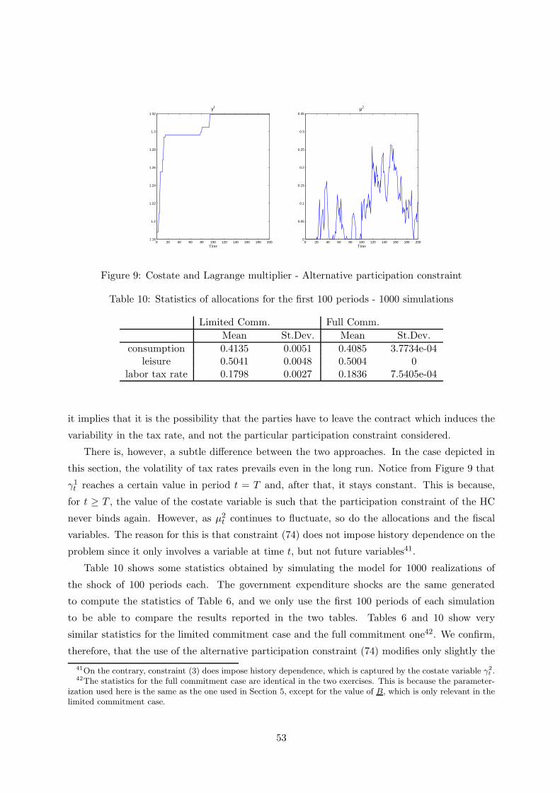
0 20 40 60 80 100 120 140 160 180 2001.18

1.2

1.22

1.24

1.26

1.28

1.3

1.32

Time

γ1

0 20 40 60 80 100 120 140 160 180 2000

0.05

0.1

0.15

0.2

0.25

0.3

0.35

Time

µ2

Figure 9: Costate and Lagrange multiplier - Alternative participation constraint

Table 10: Statistics of allocations for the first 100 periods - 1000 simulations

Limited Comm. Full Comm.

Mean St.Dev. Mean St.Dev.

consumption 0.4135 0.0051 0.4085 3.7734e-04leisure 0.5041 0.0048 0.5004 0

labor tax rate 0.1798 0.0027 0.1836 7.5405e-04

it implies that it is the possibility that the parties have to leave the contract which induces the

variability in the tax rate, and not the particular participation constraint considered.

There is, however, a subtle difference between the two approaches. In the case depicted in

this section, the volatility of tax rates prevails even in the long run. Notice from Figure 9 that

γ1t reaches a certain value in period t = T and, after that, it stays constant. This is because,

for t ≥ T , the value of the costate variable is such that the participation constraint of the HC

never binds again. However, as µ2t continues to fluctuate, so do the allocations and the fiscal

variables. The reason for this is that constraint (74) does not impose history dependence on the

problem since it only involves a variable at time t, but not future variables41.

Table 10 shows some statistics obtained by simulating the model for 1000 realizations of

the shock of 100 periods each. The government expenditure shocks are the same generated

to compute the statistics of Table 6, and we only use the first 100 periods of each simulation

to be able to compare the results reported in the two tables. Tables 6 and 10 show very

similar statistics for the limited commitment case and the full commitment one42. We confirm,

therefore, that the use of the alternative participation constraint (74) modifies only slightly the

41On the contrary, constraint (3) does impose history dependence, which is captured by the costate variable γ2t .

42The statistics for the full commitment case are identical in the two exercises. This is because the parameter-ization used here is the same as the one used in Section 5, except for the value of B, which is only relevant in thelimited commitment case.

53

0 20 40 60 80 100 120 140 160 180 200

0.175

0.18

0.185

0.19

Time

Taxes

0 20 40 60 80 100 120 140 160 180 2000.06

0.07

0.08

0.09

0.1

0.11

0.12

Time

Government Expenditure

0 20 40 60 80 100 120 140 160 180 200−0.05

0

0.05

0.1

0.15

0.2

Time

Market Value of Debt

Limited commitment Full commitment

Figure 10: Fiscal variables - Alternative participation constraint

results reported in the main text.

A.7 The International Institution Problem and the Government Problem:

Equivalence of Results

Suppose that there exists an international financial institution that distributes resources

among the HC and the RW, taking into account the aggregate feasibility constraint (14), the

implementability condition (15), and participation constraints (17) and (18). Assume for sim-

plicity that b−1 = 0. The Lagrangian associated to the international institution is

max{c1t ,c

2t ,Tt}∞t=0

∞∑

t=0

βt(ηu(c1t , l1t ) + (1 − η)u(c2t )

+µ1,t(Et

∞∑

j=0

βju(c1t+j , l1t+j) − V

1,at ) + µ2,t(B − Et

∞∑

j=0

βjTt+j)

−∆(uc1,tc1t − ul1t

(1 − l1t )) − ψt(c1t + c2t + g − (1 − l1t + y)))

(83)

where η is the Pareto weight that the international institution assigns to the HC and y

is a fixed endowment that households of the RW receive every period. Since by assumption

households in the RW are risk-neutral, u(c2t ) = c2t . The feasibility constraint of the RW implies

that c2t = y − Tt. Substituting this into (83) and applying Marcet and Marimon (2009) we can

recast problem (83) as

54

max{c1t ,c

2t ,Tt}∞t=0

∞∑

t=0

βt((η + γ1,t)u(c1t , l

1t ) + (1 − η)(y − Tt)

−µ1,tV1,at + µ2,tB − γ2,tTt − ∆(uc1,tc

1t − ul1t

(1 − l1t )) − ψt(c1t + g − (1 − l1t + Tt))

(84)

Dividing each term by η does not change the solution, since η is a constant. Letγi

t

η≡ γit, for

i = 1, 2, ∆η≡ ∆ and ψt

η≡ ψt. The first-order conditions are

uc,t(1 + γ1t ) − ψt − ∆(ucc,tct + uc,t − ucl,t(1 − lt)) = 0 (85)

ul,t(1 + γ1t ) − ψt − ∆(ucl,tct + ul,t − ull,t(1 − lt)) = 0 (86)

ψt =1 − η

η+ γ2

t (87)

where ct ≡ c1t . Calling λ ≡ 1−ηη

makes the system of equations (85)-(87) coincide with

(19)-(21).

A.8 Proof of Proposition 5

First notice that when we introduce (45) as one of the constraints of the Ramsey planner’s

problem, the problem becomes non-recursive because future endogenous variables appear in a

constraint valid in period t. Once more, we need to apply the recursive contract’s approach of

Marcet and Marimon (2009) to write a recursive problem which solution coincides with the one

of the original problem. The Lagrangian of this new problem can be written as

L =E0

∞∑

t=0

βt{u(c1t , l1t ) − (∆ + Λ1,t)(uc1,tc

1t − ul1,t(1 − l1t )) + λ1,tBt−1(gt) − λ2,t(A

1t (gt+1)

− Z1t (gt+1)) + λ3,t(1 − l1t −

∑

gt+1

qtZ1t (gt+1) + Z1

t−1(gt) − c1t − gt) + ∆b−1uc1,0}

where Λ1,t = Λ1,t−1 + λ1,t is a costate variable representing the sum of all past Lagrange

multipliers λ1 attached to constraint (45), and its initial condition is Λ1,−1 = 0. This costate

variable keeps track of all past periods in which the constraint on the value of the domestic debt

has been binding.

The optimality conditions are

uc1,t − (∆ + Λ1,t)(ucc1,tc1t + uc1,t − uc1l,t(1 − lt)) = λ3,t (88)

ul1,t − (∆ + Λ1,t)(uc1l,tc1t + ul1,t − ull1,t(1 − l1t )) = λ3,t (89)

55

qt(gt+1) =βλ3,t+1π(gt+1|gt) + λ2,t

λ3,t(90)

The problem of households in the RW and the optimality conditions associated to it are

given by (30)-(32) and (33)-(35), respectively.

Following Alvarez and Jermann (2000), we prove the proposition by construction. We con-

sider three possible scenarios:

1. Neither the HC’s nor the RW’s participation constraints are binding in t+ 1, ∀g′ = gt+1

2. The RW’s participation constraint is binding in t+ 1 for g′ = gt+1

3. The HC’s participation constraint is binding in t+ 1 for g′ = gt+1

1. Neither the HC’s nor the RW’s participation constraints are binding in t+ 1,

∀g′ = gt+1

Assume for simplicity that neither the HC not the RW have ever been borrowing con-

strained and, consequently, Λ1,t = 0. Set debt limits A1t (g

′), A2t (g

′) and Bt(g′) to be very

large in absolute value such that constraints (29), (32) and (45) do not bind for g′ = gt+1.

Then multipliers λ1,t+1 = λ2,t = ω2t = 0. Given the allocations, equations (33) and (90)

define prices. Notice that, from these two equations and the optimality conditions (88)

and (89), it has to be the case that c1t = c1t+1 and lt = lt+1. The allocations of the prob-

lem of Section 3 satisfy these conditions. Notice also that, given the assumptions made,

γ1t = γ2

t = µ1t+1 = µ2

t+1 = 0. Finally, from the optimality conditions of the two problems,

(19)-(21) and (88)-(90), it is easy to see that it has to be the case that λ3,t = λ. The initial

level of international bonds Z1−1 = −Z2

−1 is chosen so that this equality holds.

2. The RW’s participation constraint is binding in t+ 1 for g′ = gt+1

From the definition of high implied interest rates, and given the allocations, the price of

the bond is determined by equation (38). From equations (33) and (90), it is clear that the

borrowing constraint of the RW is binding, while the borrowing constraint of the HC is

not. Therefore, we set the debt limit A2t (g

′) to be equal to the holding of the corresponding

bond. We will explain later how such holdings are determined. The rest of the debt limits,

A1t (g

′) and Bt(g′), are again set to be very large in absolute value so that constraints

(29) and (45) do not bind for g′ = gt+1. From (19)-(21) and (88)-(90), we know that

λ3,t+1 > λ3,t because γ2t+1 > 0, which is exactly what the pricing equation is reflecting.

56

3. The HC’s participation constraint is binding in t+ 1 for g′ = gt+1

From the definition of high implied interest rates, and given the allocations, the price of

the bond is determined by equation (38). From equations (33) and (90), it is clear that the

borrowing constraint of the HC is binding, while the borrowing constraint of the RW is

not. Also, given the allocations, it is clear from (19)-(21) and (88)-(90) that λ3,t+1 < λ3,t

because γ1t+1 > 0. From equation (90) we can conclude that λ2,t > 0. Consequently, we set

the debt limit A1t (g

′) to be equal to the holding of the corresponding international bond.

Moreover, we set the limit Bt(g′) to be equal to the holding of the domestic bond, which

is already known from the allocations of Section 3. The debt limit A2t (g

′) is set to be very

large in absolute value so that constraint (32) does not bind.

Notice that equations (19) and (20) imply that:

uc,t(1+γ1t )−∆(ucc,tct+uc,t−ucl,t(1− lt)) = ul,t(1+γ1

t )−∆(ucl,tct+ul,t−ull,t(1− lt)) (91)

On the other hand, equations (88) and (89) imply:

uc1,t−(∆+Λ1,t)(ucc1,tc1t+uc1,t−uc1l,t(1−lt)) = ul1,t−(∆+Λ1,t)(uc1l,tc

1t+ul1,t−ull1,t(1−l

1t ))

(92)

If we did not introduce a limit of the value of domestic debt, then the allocations that

solve (91) would never solve (92), because the possibility of default in the first case changes

the marginal rate of substitution between consumption and labor, but the binding limits

on international debt alone would not do so in the second case. Therefore, we need to

introduce a limit on the value of domestic debt as well.

Finally, we need to determine the holdings of the corresponding international bonds. From

the budget constraints of the HC and the RW, (41) and (31) respectively, and given prices

and allocations, iterate forward to obtain the holding of the international bond for each possible

realization of the public expenditure shock gt. This ensures that c1t , lt and c2t are budget feasible.

It is easy to see that, if constructed in this way, Z1t (g

′) + Z2t (g

′) = 0 ∀g′.

A.9 Computational algorithm

Following Christiano and Fisher (2000), we solve the model by a projection method in which

we parameterize the expectations associated to the two participation constraints (17) and (18).

57

We use linear splines to approximate the expectations. Our problem entails three state variables

corresponding to the government expenditure shock and the two costate variables associated to

the participation constraints of the HC and the RW respectively. We construct the grid for

the approximation by considering 4 points for each state variable, which implies that the grid

has 64 points in total. The intervals in which we approximate the solution are the following:

gt ∈ [g − 2σg, g + 2σg], γ1t ∈ [0, 1.2] and γ2

t ∈ [0, 0.3].

The algorithm is as follows:

1. For a given guess for ∆ and λ, obtain the initial guess of the parameters that approximate

the expectations in the left hand side of equations (17) and (18) by considering that the

participation constraints are never binding. The allocations are obtained by solving the

optimality conditions for γ1t = γ2

t = 0. Once we have the allocations, we can write the

expectations recursively. In particular, consider the expectation in the left-hand side of the

participation constraint for the HC. Then, Et∑∞

j=0 βju(ct+j , lt+j) ≡ V (gt, γ

1t−1 = 0, γ2

t−1 =

0) and

V (gt, γ1t−1 = 0, γ2

t−1 = 0) = u(ct, lt) + βEtV (gt+1, γ1t = 0, γ2

t = 0) (93)

For a given guess for V (gt, γ1t−1 = 0, γ2

t−1 = 0) and for the allocations previously ob-

tained, we iterate on (93) to obtain Et∑∞

j=0 βju(ct+j , lt+j). We do the same to obtain

Et∑∞

j=0 βjTt+j ≡ U(gt, γ

1t−1 = 0, γ2

t−1 = 0).

(a) Given the guess for the parameters that approximate expectations and the guesses for

∆ and λ, we obtain the equilibrium allocations in the following manner: assume that

neither the participation constraint of the HC nor the one of the RW bind in period

t. Then µ1t = µ2

t = 0. Then compute ct, lt and Tt from the optimality conditions of

the problem:

uc,t(1 + γ1t−1) − ∆(ucc,tct + uc,t − ucl,t(1 − lt)) = λ+ γ2

t−1

ul,t(1 + γ1t−1) − ∆(ucl,tct + ul,t − ull,t(1 − lt)) = λ+ γ2

t−1

ct + gt = (1 − lt) + Tt

(b) Given µ1t = µ2

t = 0, compute a large grid at t+1 for every possible realization of gt+1,

given gt. Then compute V (gt+1, γ1t = γ1

t−1, γ2t = γ2

t−1) and U(gt+1, γ1t = γ1

t−1, γ2t =

γ2t−1). Compute

58

A1t = Et

∞∑

j=0

βju(ct+j , lt+j) = u(ct, lt) + βEtV (gt, γ1t = γ1

t−1, γ2t = γ2

t−1)

A2t = Et

∞∑

j=0

βjTt+j = Tt + βEtU(gt+1, γ1t = γ1

t−1, γ2t = γ2

t−1)

(c) Using A1t , check whether the participation constraint of the HC is satisfied or not. If

it is, proceed to the next step, otherwise recompute the allocations ct, lt, Tt and µ1t

from optimality conditions

uc,t(1 + γ1t−1 + µ1

t ) − ∆(ucc,tct + uc,t − ucl,t(1 − lt)) = λ+ γ2t−1

ul,t(1 + γ1t−1 + µ1

t ) − ∆(ucl,tct + ul,t − ull,t(1 − lt)) = λ+ γ2t−1

ct + gt = (1 − lt) + Tt

u(ct, lt) + βEtV (gt, γ1t = γ1

t−1 + µ1t , γ

2t = γ2

t−1) = V a(gt)

(d) Using A2t , check whether the participation constraint of the RW is satisfied or not. If

it is, proceed to the next step, otherwise recompute the allocations ct, lt, Tt and µ2t

from optimality conditions

uc,t(1 + γ1t−1) − ∆(ucc,tct + uc,t − ucl,t(1 − lt)) = λ+ γ2

t−1 + µ2t

ul,t(1 + γ1t−1) − ∆(ucl,tct + ul,t − ull,t(1 − lt)) = λ+ γ2

t−1 + µ2t

ct + gt = (1 − lt) + Tt

Tt + βEtU(gt+1, γ1t = γ1

t−1, γ2t = γ2

t−1 + µ2t ) = B

(e) Given ct, lt, Tt, µ1t and µ2

t , compute a large grid at t+1 for every possible realization

of gt+1, given gt. Then compute V (gt+1, γ1t = γ1

t−1, γ2t = γ2

t−1) and U(gt+1, γ1t =

γ1t−1, γ

2t = γ2

t−1). Compute

V ∗(gt, γ1t−1, γ

2t−1) = u(ct, lt) + βEtV (gt+1, γ

1t = γ1

t−1, γ2t = γ2

t−1)

U∗(gt, γ1t−1, γ

2t−1) = Tt + βEtU(gt+1, γ

1t = γ1

t−1, γ2t = γ2

t−1)

(f) Compute residuals

rV = V ∗(gt, γ1t−1, γ

2t−1) − V (gt, γ

1t−1, γ

2t−1) (94)

59

rU = U∗(gt, γ1t−1, γ

2t−1) − U(gt, γ

1t−1, γ

2t−1) (95)

(g) Solve the system of nonlinear equations given by (94) and (95) using a nonlinear

equation solver such as Broyden’s algorithm.

2. Once the equilibrium parameters for a guess of ∆ and λ have been obtained, compute the

allocations at t = 0 from the optimality conditions of the problem. Notice that the FOCs

with respect to c0 and l0 are:

uc,0(1 + γ10) − ∆(ucc,0c0 + uc,0 − ucl,0(1 − l0) − ucc,0b−1) = λ+ γ2

0

ul,0(1 + γ10) − ∆(ucl,0c0 + ul,0 − ull,0(1 − l0) − ucl,0b−1) = λ+ γ2

0

Notice that, as before, it is necessary to check whether either the participation constraint

of the HC or of the RW are violated. In such a case, the allocations have to be recalculated

to make the corresponding participation constraint bind.

3. Compute residuals

r∆ = E0

∞∑

t=0

βt(uc,tct − ul,t(1 − lt)) − uc,0b−1 (96)

rλ = E0

∞∑

t=0

βtTt (97)

4. Solve the system of nonlinear equations given by (96) and (97) using a fine grid search for

∆ and λ.

60