fibre-generated point processes and fields of orientations

The Annals of Applied Statistics2012, Vol. 6, No. 3, 994–1020DOI: 10.1214/12-AOAS553© Institute of Mathematical Statistics, 2012

FIBRE-GENERATED POINT PROCESSES AND FIELDSOF ORIENTATIONS

BY BRYONY J. HILL, WILFRID S. KENDALL AND ELKE THÖNNES

University of Warwick

This paper introduces a new approach to analyzing spatial point dataclustered along or around a system of curves or “fibres.” Such data arise incatalogues of galaxy locations, recorded locations of earthquakes, aerial im-ages of minefields and pore patterns on fingerprints. Finding the underlyingcurvilinear structure of these point-pattern data sets may not only facilitate abetter understanding of how they arise but also aid reconstruction of missingdata. We base the space of fibres on the set of integral lines of an orientationfield. Using an empirical Bayes approach, we estimate the field of orientationsfrom anisotropic features of the data. We then sample from the posterior dis-tribution of fibres, exploring models with different numbers of clusters, fittingfibres to the clusters as we proceed. The Bayesian approach permits inferenceon various properties of the clusters and associated fibres, and the results per-form well on a number of very different curvilinear structures.

1. Introduction. In this paper we introduce a new empirical Bayes approachconcerning point processes that are clustered along curves or “fibres,” with addi-tional background noise.

In nature such point patterns often arise when events occur near some la-tent curvilinear generating feature. For example, earthquakes arise around seismicfaults which lie on the boundaries of tectonic plates and hence are naturally curvi-linear. Similarly, sweat pores in fingerprints lie on the ridges of the finger, whichpossess a curvilinear structure. Figure 1 presents these data together with two sim-ulated examples of point patterns clustered around underlying families of curveswith additional background noise. Identification of curvilinear elements and elu-cidation of their relationship with the point data is both an interesting theoreticalproblem and a useful tool for gaining understanding of the origins of the data. Italso provides a technique for reconstruction of missing data.

The model introduced here describes families of nonintersecting curves via afield of orientations (a map υFO :W → [0, π) assigning an undirected orientationto each point in the window). The curves are produced as segments of streamlinesintegrating the field of orientations. We say that a curve integrates the field oforientations if the curve is continuously differentiable and of unit speed, and if itstangent agrees with the field of orientations at each point. The term streamline is

Received September 2011; revised February 2012.Key words and phrases. Markov chain Monte Carlo, spatial birth–death process, earthquakes, em-

pirical Bayes, fibre processes, field of orientations, fingerprints, spatial point processes, tensor fields.

994

http://www.imstat.org/aoas/

http://dx.doi.org/10.1214/12-AOAS553

http://www.imstat.org

FIBERS, POINT PROCESSES, FIELDS OF ORIENTATIONS 995

(a) (b)

(c) (d)

FIG. 1. Four examples of point patterns clustered around latent curvilinear features with back-ground noise. (a) Simulated point pattern. (b) Simulated point pattern described in Stanford andRaftery (2000). (c) Earthquake epicenters in the New Madrid region. Data is taken from CERI (Cen-ter for Earthquake Research and Information). (d) Pores along ridges of a portion of the fingerprinta002–05 from the NIST Special Database 30 [Watson (2001)].

used to describe a curve which integrates the field of orientations and has no endpoints in the interior of the window W \ ∂W .

We choose to use a variant on an empirical Bayes approach to estimate the fieldof orientations, since a fully Bayesian approach would involve infinite-dimensionaldistributions and be very computationally intensive. The empirical Bayes compo-nent consists of estimation of the field of orientations from the data via a tensorfield as detailed in Section 4.1. In the following, a tensor field is represented byassignation of a symmetric nonnegative definite matrix to each point of the planarwindow. Tensor fields of this kind play an important role in diffusion tensor imag-

996 B. J. HILL, W. S. KENDALL AND E. THÖNNES

ing [DTI, see Le Bihan et al. (2001)]. The field of orientations is constructed sim-ply by calculating the orientations of the representative matrices’ principal eigen-vectors; singularities in the field of orientations correspond to points where thereis equality of the two eigenvectors.

We show how properties of the underlying distribution of fibres can be estimatedusing Monte Carlo techniques applied to the spatial point data. Our approach hasthe advantage that it can be used to quantify uncertainty on a range of parametersand does so effectively for different types of curvilinear structure. The use of a fieldof orientations to identify fibres leads to a strong performance on data such as thatshown in Figure 1(d), where there is noticeable alignment of points perpendicularto the fibres.

1.1. Potential applications. Point patterns with a latent curvilinear structurearise in many different areas of study.

In seismology, epicenters of earthquakes are typically densely clustered aroundseismic faults. The earthquake data from the New Madrid region as shown in Fig-ure 1(c) consists of one short dense cluster of points, one longer rather sparsecluster, both connected, and a relatively small number of “noise” points scatteredover the window. The New Madrid earthquake data is considered in Stanford andRaftery’s (2000) approach to detecting curvilinear features.

In cosmology, galaxies appear to cluster along inter-connected filaments form-ing a three-dimensional web-like structure with large voids between the fila-ments. There is interest in identifying the nature of the filaments [see, e.g., Stoica,Martínez and Saar (2007)]. There is also evidence that these galaxies form surfacesor “walls” in some regions. This suggests the exciting challenge of extending ourmodel to include two-dimensional surfaces in three-dimensional space.

A further application is that of sweat pore patterns on fingerprint ridges [seeFigure 1(d)]. Sweat pores are tiny apertures along the ridges where the ducts of thesweat glands open. Robust inference of the ridge structure from the pore patternhas potential for aiding reconstruction of patchy fingerprints and may also allowfor more efficient storage of fingerprints in very large databases. The underlyingcurve structure is a dense set of locally parallel curves along which pores are lo-cated, usually very close to the center of the ridges. The noise arises mostly fromartifacts in the automatic extraction of pores from the image.

An issue with fingerprint pore data is that pores usually align across the ridgesas well as along them. This can complicate the reconstruction of ridges, as thedominant orientation is less clear. We overcome this issue by constructing a smoothtensor field which extrapolates dominant orientation estimates over the regions ofdirectional ambiguity.

1.2. Background. An existing method of estimating the curves in the underly-ing structure of a point process is Stanford and Raftery’s (2000) use of principal


curves (a nonlinear generalization of the first principal component line). An EM-algorithm is used to optimize the model over a variety of choices of smoothnessparameter and number of components. An optimal choice of smoothness and num-ber of components is then selected using Bayes factors. This technique generallyperforms very well; however, it is sensitive to the initial clustering of the data andtherefore has difficulties reconstructing fibres in some regions where fibres may beexpected but signal points are absent [e.g., the fingerprint pore data—Figure 1(d)].

A piecewise linear “Candy model” (or “Bisous model” in three dimensions) isused by Stoica, Martínez and Saar (2007) to model filaments in galaxy data. Theycompare the empirical densities of galaxies within concentric cylinders and thusdelineate these filaments. This approach is restricted to piecewise linear fibre mod-els where the deviation of points from fibres follows a uniform distribution overa thin cylinder centered along the fibre. Sufficient statistics of the model for datawith filamentary structure are then compared to sufficient statistics on structurelessdata sets; see Stoica et al. (2005) and Stoica, Martínez and Saar (2007, 2010).

Density estimates of the point pattern can be obtained using techniques such askernel smoothing. Fibres can be directly estimated from this density; an exampleof this can be seen in Genovese et al. (2009) where steepest ascent paths along thedensity estimate are constructed and the density of these paths is analyzed.

A further approach discussed in Barrow, Bhavsar and Sonoda (1985) is basedon construction of the minimal spanning tree of the set of points. In three dimen-sions this gives a useful insight into the overall characteristics of the filamentarystructure.

The method presented in August and Zucker (2003) is based on a random curvemodel in which curvature is defined as a Brownian motion. The resulting model isused to enhance contours in the output of edge operators applied to digital imagesand thus to data in which signal points are dense along curvilinear structures.

The treatment advocated here is also based on the formulation of a generalmodel for families of curves and the point patterns clustered around them. In con-trast to August and Zucker (2003), curves are modeled as segments of streamlinesintegrating a smooth field of orientations which encourages interpolations over ar-eas of missing data. The prior model for the orientation field is derived via an em-pirical Bayes step. Then birth–death MCMC is used to sample from the posteriordistribution of the fibres. The model formulation itself uses the initial exploratorywork of Su et al. (2008) [see also Su (2009)], which focused on the fingerprint poredata and described the use of tensor fields for estimating dominant orientations inspatial point data.

1.3. Problem definition. In particular, we are interested in modeling a randompoint process � viewed in a planar window W ⊂ R

2; we write the observed part ofthe point process as W ∩ � = {y1, . . . , ym} for some arbitrary ordering of points.The point process arises from a mixture of homogeneous background noise andan unknown number of point clusters, each clustered along a curve, henceforth


called a fibre. Thus a fibre is a one-dimensional object, a smooth curved segment,embedded in a higher-dimensional space (the space containing the point process).Random sets of fibres or “fibre processes” are discussed in Stoyan, Kendall andMecke (1995) and Illian et al. (2008).

Having specified an appropriate model, we must identify a suitable method ofanalysis of the posterior distribution of fibres given a data set of spatial point loca-tions {y1, . . . , ym} over the window W .

1.4. Plan of paper. The paper is laid out as follows. The following sectiongives an overview of the model proposed in this paper. Details of the underlyingprobability model are given in Section 3. The empirical Bayes method of estimat-ing an appropriate field of orientations is outlined in Section 4. Section 5 presentsa method of sampling from the posterior distribution of the fibres given the pointpattern data using Monte Carlo methods. This is implemented for a number ofexamples in Section 6. In the final section we compare this model to other ap-proaches, discuss some known issues of implementation and statistical analysis,and note possible directions in which this model might be extended.

2. Basic considerations. We use a Bayesian hierarchical model to describethe relationship between the points and the fibres.

2.1. Points. A natural choice is to model the spatial point process as a mixedPoisson process or “Cox process” driven by a random fibre process. By this wemean that the points arise independently and are associated in some way witha random fibre—typically clustered around it. Such a point process is called a“fibre-process generated Cox process;” see Illian et al. (2008).

In our model we do associate points with particular fibres but we remove thePoissonian character of the distribution of points along fibres, replacing this bya renewal process based on Gamma distributions for interpoint distances. This al-lows us to model a tendency to regularity in the way in which points are distributedalong a fibre but includes the Poissonian case with exponentially distributed inter-point distances.

2.2. Fibres. In contrast to previous work, in which curves are often con-structed as splines fitted to the data, we define them as integral curves of a fieldof orientations. This means that at any point on a fibre, the tangent to the fibreagrees with the field of orientations at that point. Note that a field of orientationsis equivalent to a vector field except that each point in the field is assigned a direc-tionless orientation. An instance of a random field of orientations ϒFO is writtenas υFO :W → [0, π), where [0, π) represents the space of planar directions (with0 and π identified).

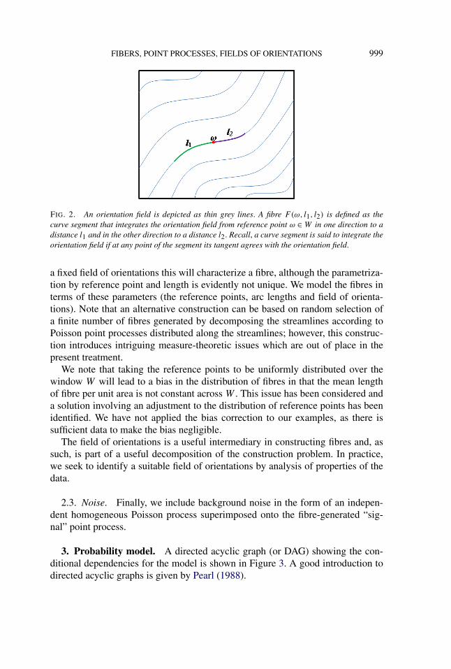
The simplest way to determine a fibre F is to choose a reference point ω ∈ W

on the fibre and specify the two arc lengths l1, l2 ∈ R+ of F \{ω}; see Figure 2. For


FIG. 2. An orientation field is depicted as thin grey lines. A fibre F(ω, l1, l2) is defined as thecurve segment that integrates the orientation field from reference point ω ∈ W in one direction to adistance l1 and in the other direction to a distance l2. Recall, a curve segment is said to integrate theorientation field if at any point of the segment its tangent agrees with the orientation field.

a fixed field of orientations this will characterize a fibre, although the parametriza-tion by reference point and length is evidently not unique. We model the fibres interms of these parameters (the reference points, arc lengths and field of orienta-tions). Note that an alternative construction can be based on random selection ofa finite number of fibres generated by decomposing the streamlines according toPoisson point processes distributed along the streamlines; however, this construc-tion introduces intriguing measure-theoretic issues which are out of place in thepresent treatment.

We note that taking the reference points to be uniformly distributed over thewindow W will lead to a bias in the distribution of fibres in that the mean lengthof fibre per unit area is not constant across W . This issue has been considered anda solution involving an adjustment to the distribution of reference points has beenidentified. We have not applied the bias correction to our examples, as there issufficient data to make the bias negligible.

The field of orientations is a useful intermediary in constructing fibres and, assuch, is part of a useful decomposition of the construction problem. In practice,we seek to identify a suitable field of orientations by analysis of properties of thedata.

2.3. Noise. Finally, we include background noise in the form of an indepen-dent homogeneous Poisson process superimposed onto the fibre-generated “sig-nal” point process.

3. Probability model. A directed acyclic graph (or DAG) showing the con-ditional dependencies for the model is shown in Figure 3. A good introduction todirected acyclic graphs is given by Pearl (1988).


FIG. 3. Directed acyclic graph (DAG) of model: arrows indicate conditional dependencies, ele-ments in squares are deterministically calculated or constant, while those in circles are randomvariables. For simplicity we have not included reference to hyperparameters λ, κ , η, αsignal andβsignal.

3.1. Fibres. Henceforth let F = {F1, . . . ,Fk} denote k random fibres. As out-lined earlier and illustrated in Figure 2, the fibre Fj is determined by a referencepoint ωj and arc lengths lj,1, lj,2. It is also written Fj = Fj (ωj , lj , νFO) [wherelj = (lj,1, lj,2)] to indicate that it is a deterministic function of ωj and lj once νFOis given. For the list of reference points we write ω = {ω1, . . . ,ωk}, and the arclength vectors are given by l = {l1, . . . , lk}. We use lj,T = lj,1 + lj,2 as a shorthandfor the total arc length of the j th fibre. Note that in general the orientation fieldυFO may possess singularities, which would constrain the choice of the lengthslj = (lj,1, lj,2); however, this does not arise in our examples.

3.2. Signal points. Points from the observed pattern may be either signal ornoise. Signal points are typically clustered around fibres. The model we use as-signs an anchor point pi on some fibre to each data point yi . The data point isthen displaced from pi by an isotropic bivariate normal distribution [i.e., yi ∼MVN(pi, σ

2dispI2), where I2 is the 2 × 2 identity matrix].


The fibre on which pi is located is determined by an auxiliary variable Xi , soXi = j if and only if pi ∈ Fj . The pi’s on the j th fibre are spaced such that thevector of arc-length distances between adjacent points is proportional to a Dirich-let distributed random variable. Setting an appropriate parameter for the Dirichletdistribution will encourage points to be either evenly spread, clustered along thefibre, or placed independently at random along the fibre.

The probability that point yi is allocated to the j th fibre (Xi = j ) is proportionalto the total length of fibre Fj . This ensures that the mean points per unit streamlineremains approximately constant.

3.3. Noise points. Noise is then added as a homogeneous Poisson process.This is included in the model by first allocating each point yi to noise or signal(stored in auxiliary variable Zi = 1 or 0 for signal or noise, resp.). Point yi isallocated to signal independently of the allocations of all other points. The priorprobability that yi is allocated to signal is given by εi . If the point is signal, thenits location is distributed as outlined in the previous subsection. Otherwise, if thepoint is noise, it is distributed uniformly across the window W .

3.4. Total number of points. The total number of points m is assumed to bePoisson distributed. The mean total number of points μtotal is defined to be equalto some function of μsignal, the mean number of signal points, and ρ, a parametergoverning the number of noise points. For the sake of simplicity we set ρ to bethe prior assumption on the proportion of the total points that are noise pointsand define μtotal = μsignal/(1 − ρ). The mean number of signal points μsignal isassumed to be proportional to the total sum of the fibre arc lengths. Hence, m isassumed to be Poisson distributed with mean

μtotal =(

k∑j=1

(lj,T )

)η

1 − ρ,(1)

where ρ = βsignal/(αsignal + βsignal) is the prior estimate of the proportion of pointsthat are signal and η is a density parameter.

The assumption that the mean number of noise points is proportional to themean total number of points (and the fibre length) is particularly well suited to thefingerprint example [see Section 6.3], where noise points arise as artifacts of thepore detection process along the fingerprint ridges. Implementation of alternativerelationships between the mean number of signal and noise points would be astraightforward matter.

3.5. Priors. In the examples given in the next Section 6 we use the followingpriors:

P(l|k,λ) =k∏

j=1

P(lj,1|λ)P (lj,2|λ) where lj,· ∼ Exp(1/λ),


P(ω|k) =k∏

j=1

P(ωj ) where ωj ∼ Uniform(W),

P (k|κ) ∼ Poisson(κ),

P (ε|αsignal, βsignal) =m∏

i=1

P(εi |αsignal, βsignal)

where εi ∼ Beta(αsignal, βsignal).

Here m is the total number of points in {y1, . . . , ym}.The above prior models are common, parsimonious choices that appear flexible

enough for a range of applications including the examples considered in Section 6.However, if application-specific prior information suggests alternative prior mod-els, then these can be accommodated in the presented framework.

3.6. Posterior. We are interested in the posterior distribution of fibres (andvarious other parameters) given a particular instance of the point process. Thisposterior is given by

π(F, l,ω, k, υFO, ε,Z,X,p)

= P(F, l,ω, k, υFO, ε,Z,X,p|y)

∝ P(F, l,ω, k, υFO, ε,Z,X,p)(2)

× L(F, l,ω, k, υFO, ε,Z,X,p|y)

= P(l|k)P (ω|k)P (k)P (υFO)P (ε)P (Z|ε)× P(X|Z, l)P (p|F,X)L(F, l,ω, k, υFO, ε,Z,X,p|y).

Here P(·) indicates a prior distribution. We omit P(F|l1, l2,ω, υFO), as it is deter-ministically calculated.

Section 5 describes how to sample from this posterior distribution using Markovchain Monte Carlo techniques.

3.7. Computational simplifications. Computer implementation makes it nec-essary to represent the field of orientations by a discrete structure. We adopt thesimple approach of estimating the field of orientations at a dense regular grid ofpoints over W . Integral curves are calculated stepwise by estimating the orienta-tion at a point by its value at the nearest evaluated grid point and extending thecurve a small distance in that direction. Note that the choice of direction (fromthe two available for each orientation) is made so that the angle between adjacentlinear segments is greater than π/2.

Consequently, fibres are stored as piecewise-linear curves and further calcula-tions are performed on these approximations. Of course, this discretization can bearbitrarily reduced (at a computational cost) to improve the accuracy of the ap-proximation.


4. Construction of field of orientations. We must of course identify amethod for calculating the field of orientations. It is computationally advantageousto generate a field of orientations which is likely to contain (be integrated by) fibresthat fit the data well (produce a high likelihood). The most natural way to do thisis to base the calculation of the field of orientations on the data, using an empiri-cal Bayes technique. The use of empirical Bayes to find the prior for the field oforientations distribution means that aspects of the prior, or parameters of the prior,are estimated from the data.

An alternative approach would be to use a fully Bayesian model, where wewould treat the field of orientations as an independent random variable ϒFO. Wewould then need to identify its state space and a corresponding σ -algebra, tran-sition kernel and prior on this state space. These could be derived from randomfield theory [see, e.g., Adler and Taylor (2007)], using an appropriate covariancefunction to maintain smoothness in the field of orientations, however, there area number of issues with this approach. In practice, one may expect the task ofsampling a random field of orientations to be computationally expensive, partic-ularly if the covariance function does not have a simple form (as is likely in thismodel). Calculations relating to the conditional distribution of the field of orien-tations given the fibres are likely to lead to unfeasible computational complexity.A further issue is that this approach leads to a huge space of possible fibres, result-ing in corresponding difficulties in ensuring this space is properly explored. Useof the information given in the data will help to limit this space to a more easilyexplorable restricted class of suitable fields of orientations.

Here we use the data to make local orientation estimates and smooth these toproduce a field of orientations estimator. As we are specifically interested in orien-tation estimates arising from the signal data, we can choose to weight the contri-bution of each point to the field of orientations estimator by how likely it is to benoise or signal.

Estimation of a field of orientations given that y1, . . . , ym are all signal pointsis outlined in the following section. Section 4.2 shows how to extend this to takeaccount of the information given in the vector of probabilities that points are signal(ε1, ε2, . . . , εm).

4.1. Estimation for all signal points. The mapping and tensor method de-scribed in Su et al. (2008) [and further discussed in Su (2009)] is applied to thepoint pattern to construct a tensor at each point. To this we apply a Gaussian ker-nel smoothing in the log-Euclidean metric to construct a tensor field. The tensorfield is represented by an assignation to each point of a 2 × 2 nonnegative defi-nite matrix whose principal eigenvector indicates the dominant orientation at thatpoint; the relative magnitude of the eigenvalues indicates the strength of the dom-inant orientation. The field of orientations assigns the orientation of this principaleigenvector to each respective point. If the principal eigenvector is not unique at


a certain point (which is to say that the eigenvalues are equal there), then thatindicates a singularity in the field of orientations.

Three-dimensional tensor fields of this kind are commonly used in diffusiontensor imaging (DTI) to understand brain pathologies such as multiple sclerosis,schizophrenia and strokes. DTI is used to analyze images of the brain collectedfrom magnetic resonance imaging (MRI) machines. The MRI scan detects diffu-sion of water molecules in the brain and uses the data to infer the tissue structurethat limits water flow. The three-dimensional diffusion tensor describes the orien-tation dependence of the diffusion. Roughly speaking, the eigenvalues indicate ameasure of the proportion of water molecules flowing in the associated eigenvectordirection. For more information on DTI see, for example, Le Bihan et al. (2001)and Li et al. (2007).

Let y1, . . . , ym denote the spatial data points. A tensor is constructed at a pointyj using a nonlinear transformation applied to the vectors vi = (vi

1, vi2) = −−→yjyi for

i �= j [Su et al. (2008), Su (2009)]. Specifically,

vi = (vi1, v

i2) = exp

(−((vi

1)2 + (vi

2)2)

2σ 2FO

)(vi

1, vi2)√

(vi1)

2 + (vi2)

2,(3)

where σFO is a scaling parameter.The tensor at yj is then represented by

T0(yj ) = ∑i �=j

(vi1, v

i2)

T(vi1, v

i2).(4)

The result of the above method is to produce a set of 2 × 2 matrices locatedover a sparse set of locations. In order to create a field of orientations, we mustthen interpolate to get a tensor field. Thus, we use the orientation of the principaleigenvector, where defined, to construct a field of orientations.

Interpolation of tensors inevitably requires a notion of tensor metric. We elect towork in the log-Euclidean metric [see Arsigny et al. (2006)]. For an extended ac-count of tensor metrics see Dryden, Koloydenko and Zhou (2009). Log-Euclideancalculations are simply Euclidean calculations on the tensor logarithms which aretransformed back to tensor space by taking the exponential. The tensors arising inthis study can all be represented by positive definite matrices. Tensor logarithmsare therefore well defined as logarithms of these matrices. However, the matrixcalculated in (4) will have a zero-eigenvalue if the points are collinear, and there-fore not be positive definite. If all points are truly collinear, then our approachbreaks down—and indeed the method is not intended for such noise-free data sets.The more common situation is that one vector vi dominates the tensor represen-tation as calculated in (4) due to the relative distances between points. Typicallythis occurs if two points are close while other points are far from the pair. Due to


rounding errors, the contribution of other points to the matrix becomes zero, andthe two remaining points are collinear by definition. In order to avoid an error inthe log-Euclidean calculation, if a tensor has at least one zero-eigenvalue, then itis replaced by the “uninformative” identity matrix, suggesting a lack of directionalinformation. Thus, we take a conservative approach that excludes any potentiallymisleading directional information.

We calculate the interpolated tensor field ThFO(x) for (x ∈ W) as a kernelsmoothing procedure, using a Gaussian kernel f with variance parameter h2

FO inthe log-Euclidean metric. Hence, when the smoothing parameter hFO is positive,hFO > 0,

ThFO(x) = exp(∑

yi∈{y1,...,ym} f (dist(x, yi)) log(T0(yi))∑yi∈{y1,...,ym} f (dist(x, yi))

).(5)

The field of orientations υFO(y1, . . . , ym;hFO)(x) for x ∈ W is then defined tobe equal to tan−1(v1(x)/v2(x)), where (v1(x), v2(x)) is the principal eigenvectorof the matrix representation of ThFO(x).

In most instances this procedure will give a good estimation of a suitable fieldof orientations for modeling the point process with integral fibres. The smoothingmethod has the drawback that it can create a bias around areas of high curvature(rapidly varying orientation) in the field of orientations. Potential solutions havebeen analyzed and found to perform well. The magnitude of the bias was found tobe proportional to the smoothing parameter hFO, hence, these solutions typicallyinvolve compensating for hFO: we give two examples:

(A) We allow the smoothing parameter to vary over the window, such that lowervalues are used in areas of high point intensity. This ensures that less informationis extrapolated to regions where there is already sufficient data, and therefore lessbias occurs in those regions.

(B) We consider two instances of the field of orientations with different val-ues of smoothing parameter h′

FO and h′′FO; the unbiased estimate can be found by

extrapolating back to estimate the field of orientations with hFO = 0.

We do not go into further detail here because doing so would distract from the mainideas in this paper, but we do notice a minor effect of this bias in the examples inSection 6. Details of these bias corrections can be found in Hill (2011).

4.2. Estimation using signal probabilities. We extend this field of orienta-tions estimation to take account of the vector of probabilities that points are signal(ε1, ε2, . . . , εm) by weighting the construction of the initial tensor and also weight-ing the contribution of each initial tensor to the kernel smoothing.

Specifically, the initial tensors are represented by

T0(yj ) = ∑i �=j

(vi1, v

i2)

T(vi1, v

i2)εi(6)


for each point yj , and the tensor field becomes

ThFO(x) = exp(∑

yi∈{y1,...,ym} εif (dist(x, yi)) log(T0(yi))∑yi∈{y1,...,ym} εif (dist(x, yi))

).(7)

This weighting allows points that are more likely to be signal points to have agreater effect on the field of orientations estimation. As εi → 0 the effect of thepoint yi on the field of orientations tends to zero, whereas if εi = 1 for all i wewould be performing the calculation described in Section 4.1.

5. Sampling from the posterior distribution. We seek to infer some char-acteristics of the fibre process when only the point pattern is known. Typical at-tributes of interest include the number of fibres, where they are located/orientated,which points arose from which fibre and which points arose from backgroundnoise.

Direct inference from the model is hindered by the complexity of its hierarchi-cal structure. Hence, we choose to draw samples from the posterior distribution ofthe fibres and other variables using Markov chain Monte Carlo methods. Charac-teristics of interest can be estimated from these samples.

5.1. Hyperparameters. As a rough guideline, hyperparameters can be chosenas follows.

The prior mean number of fibres κ and the prior mean length of fibres λ can beestimated from any prior knowledge or expectations of the fibres. The deviation ofpoints from fibres σ 2

disp can be estimated using prior knowledge of fibre widths andthe approximation that 95% of points should lie within 2.45σdisp of the center of afibre. The density of points per unit length of fibre η can be similarly estimated.

Orientation field parameters hFO and σFO should be chosen to ensure the orien-tation field is smooth. These can be estimated by evaluating the orientation fieldsfor different selections of hFO, σFO and choosing from this set. If the proportion ofnoise points is approximately known, then the hyperparameters αSignal and βSignalcan be suitably estimated, however, we suggest choosing the parameters such thatαSignal, βSignal > 1 to ensure good mixing properties of the Markov chain MonteCarlo sampling algorithm. Otherwise the noise hyperparameters can be set equalto 1, indicating no prior knowledge.

Alternatively, if little prior information is known about the nature of the latentcurvilinear structure, then it would be feasible to extend the empirical Bayes stepto include the estimation of further prior parameters.

5.2. Birth–death Monte Carlo. The starting point for our algorithm is a con-tinuous time birth–death Markov chain Monte Carlo (BDMCMC) in which fibresare created and die at random times controlled by predetermined or calculatedrates. This enables exploration of a wide range of models with different numbers


of fibres, and is suited to this type of clustered data. See Møller and Waagepetersen(2004) for an introduction to spatial birth–death processes. For the sake of brevitywe present in the following the key points of the algorithm. Further details can befound in Hill (2011).

Here we choose to fix the birth rate and calculate an appropriate death rate ateach step to maintain detailed balance.

Following a birth or death we update the following auxiliary variables: Z to Z′,the indicators of the components (signal/noise) to which the points are associated;X to X′, the indicators of the fibres to which the signal points are associated; pto p′, the vector (p1, . . . , pm) where pi is the point on the fibre to which the datapoint yi is associated.

5.3. Births of fibres. Recall that the parameterization of fibres is described inSection 2.2. Birth events occur randomly at rate β . Upon the occurrence of a birth,the number of fibres is updated from k to k + 1, and a new fibre is introduced bysampling a reference point ωk+1 and lengths lk+1,1, lk+1,2 from the prior distri-butions P(ω),P (l), respectively. The new fibre Fk+1 is then calculated by inte-grating the field of orientations according to these parameters, and the set of fibresF = F1, . . . ,Fk is updated to F′ = F1, . . . ,Fk,Fk+1. In order to ensure that thedistribution of the lengths lk+1,1, lk+1,2 is independent of the respective directionsin which the field of orientations is integrated, we choose them to be independentlyand identically distributed.

Data points which are currently assigned to the noise component are reassignedto noise or signal with proposal probability dependent on the new fibre Qbirth(Z →Z′|Z,ε,Fk+1).

Finally, new values are proposed for all of X,p according to a proposal densityQ(X,p → X′,p′). For simplicity, we choose not to sample from the full condi-tional distribution of p and X, but rather from a density proportional to the likeli-hood L(p,X|y).

In full, the birth density of fibre Fk+1 including updates of auxiliary variablesto Z′,X′,p′ is given by

b(Fk+1,ωk+1, l1,k+1, l2,k+1,Z′,X′,p′)= βP (ωk+1)P (l1,k+1)P (l2,k+1)Qbirth(Z → Z′|Z, ε,Fk+1)(8)

× Q(X,p → X′,p′).

5.4. Deaths of fibres. We must calculate the death rate δj for each fibre toensure detailed balance holds. Following the death of fibre Fj , the variables F,ωand l are updated by omitting the j th term. Further, auxiliary variables Z,X and pare all updated. All points allocated to fibre Fj are now allocated to noise. We callthis trivial proposal density Qdeath(Z′|Z,X, j). Again the final step is to proposenew values for all of X and p according to proposal density Q(X,p → X′,p′).


Hence, the death rate that satisfies detailed balance for the j th fibre is given by

δj = P(l1 \ l1,j , l2 \ l2,j |k − 1)

P (L1,L2|k)

P (ω \ ωj |k − 1)

P (ω|k)

P (k − 1)

P (k)

× b(Fj ,ωj , l1,j , l2,j ,Z′,X′,p′)Qdeath(Z′|Z,X, j)Q(X,p → X′,p′)

(9)

= P(k − 1)

P (k)

βQbirth(Z′ → Z|ε,Fj )Q(X′,p′ → X,p)

Qdeath(Z′|Z,X, j)Q(X,p → X′,p′).

5.5. Additional moves. It can be desirable to add extra moves to the BDM-CMC process to improve mixing. Some possible moves which were all utilized inthe examples in Section 6 include the following:

• moving a fibre by a small amount (by perturbing the reference point),• resampling the lengths of a fibre (while keeping the reference point fixed).

Each of these events occur at some predefined rate, whence they are proposed andeither accepted or rejected according to the Metropolis Hastings probability.

We may also wish to update other model variables, giving more flexibility andimproving the algorithm’s exploration of the sample space. The additional variableupdates used in the examples in Section 6 include the following:

• proposing new signal-noise allocations of the data (Z),• proposing new signal probabilities (ε) according to nondegenerate Beta distri-

butions whose parameters depend on the current signal- noise allocations Z.This move leads to an update in the prior for the field of orientations due to theempirical Bayes step, hence, all fibres are resampled.

Details of all moves can be found in Hill (2011).Hyperprior parameters, such as the constant of proportionality η in the prior for

the Poisson-distributed number of points or σdisp governing the deviation of pointsfrom fibres, may also be updated. We have chosen not to update any hyperpriorparameters to reduce complexity of the model.

5.6. Convergence and output analysis. First recall that the signal probabilitiesε are updated according to nonsingular Beta distributions. Hence, the underlyingtensor field as defined in (7) will not become degenerate even when Z allocates allpoints to noise.

Consider the set A of states in which the fibre configuration is empty and allpoints are allocated to noise. In the following discussion we exclude any degener-ate states of equilibrium probability zero. Inspection of the algorithm shows thatthe set A can be reached from any nondegenerate state in finite time and so thebirth–death process is φ-irreducible. Recurrence can be deduced by noting that theset A is visited infinitely often; see Kaspi and Mandelbaum (1994).


We motivate a heuristic lower bound on a suitable burn-in time by consideringaspects of the prior derived after inspection of the data (e.g., σdisp, λ, κ—see Sec-tion 5.1), and estimating the number of fibre births that must occur before a fibrehas been created around each potential fibre cluster. We approximate the lowerbound by considering the number of fibre births required for this to happen aroundthe smallest suitable cluster of points.

A lower bound on half the length of the shortest suitable cluster is derived fromthe 10% quantile of an exponentially distributed random variable of rate κ/λ. Thenthe probability that a point chosen at random from W lies in a region correspondingto an actual fibre of this length (up to 2σdisp from the fibre) is approximated by

8λ log(10/9)σdisp

κ|W | .(10)

It follows that, with probability 0.99, a fibre will be proposed in the region corre-sponding to the shortest fibre within the first

log(0.01)

log(1 − 8λ log(10/9)σdisp/(κ|W |))(11)

births. Hence, we choose a burn-in time of

Tburn = max{

1500,log(0.01)

β log(1 − 8λ log(10/9)σdisp/(κ|W |))},(12)

taking 1500 as a lower bound to ensure the burn-in time remains substantial.Convergence was assessed by considering variables such as the number of fibres

k or the number of noise points and using Geweke’s spectral density diagnostic; seeBrooks and Roberts (1998). Convergence of a sequence of n samples is rejected ifthe mean value of the variable in the first n/10 samples is not sufficiently similarto the mean value over the last n/2 samples.

We also tested convergence by assessing whether the mean sum of the deathrates is approximately equal to the birth rate β . Consider δk

totaltk where δk

total is thesum of the death rates of fibres after the kth event (e.g., birth, death, etc.) and tk

is the length of algorithmic time before the next event. If the MCMC has reachedstationarity, then

Zm =∑m

k=1 δktotalt

k − mβ/(2β + radd)

σδtotalt

√m

D→ N(0,1),(13)

where σδtotalt is an estimate of the standard deviation of δktotalt

k , β is the birthrate of fibres, and radd is the sum of the rates of any additional moves imple-mented (as suggested in Section 5.5). We used this result to test the convergenceof 1/m

∑mk=1 δk

totaltk to β/(2β + radd).

Bearing in mind the complexities of the underlying model, output analysisshowed no evidence for a lack of convergence.


Outputs of various variables are recorded at random times at some constant rate.The rate of this sampling (effectively the reciprocal of the thinning of the MonteCarlo process) is chosen such that there is a low probability that any of the fibresremain unchanged between samples. The inclusion of the extra moves designedto improve mixing also helps to decrease the thinning required. The thinning ischosen approximately proportional to the number of fibres (estimated based onaspects of priors derived from inspection of the data).

6. Simulation studies and applications. The implemented algorithm runs ona continuous time scale. Events occur at a determined rate, either fixed or calcu-lated to ensure that detailed balance holds. The units for the rate of an event are“per unit of algorithm time.” The BDMCMC is then allowed to run for a largenumber of time units and samples are taken at random times (at some fixed rate).Of course, the relationship of algorithm time to actual processing time depends onhardware and implementation details. Hardware details are described below.

In each of the following examples, the birth rate and the rate of other moves(moving a fibre, adjusting lengths of a fibre, proposing a split or a join, variableupdates) were all unit rate. The only exceptions were the signal probability (ε)updates which were proposed at a rate of 0.1 per unit of time, and the recording ofoutput variables at random times whose rate varied for different data sets.

We evaluate the field of orientations over a square grid of points, each one unitlength from its four nearest neighbors. The total size of this grid is given by thedimensions of the window W .

All three examples were run on the cluster owned by the Statistics Departmentin the University of Warwick using a Dell PowerEdge 1950 server with a 3.16 GHzIntel Xeon Harpertown (X5460) processor and 16 GB fully-buffered RAM. Thealgorithm was implemented in Octave version 3.2.4.1 The total run-times on thecluster ranged from 34.7 hours for the fingerprint pore data (32,300 units of algo-rithm time) to 61.3 hours for the earthquake data set (30,000 units of algorithmtime). Due to the limitations of the current version of Octave, the benefits of aparallel implementation have not yet been explored.

Analysis has been performed on all four of the data sets shown in Figure 1.However, for the sake of brevity, we omit discussion of results for the first simu-lated point pattern [Figure 1(a)] from this paper.

6.1. Simulated example. Figure 4(a) shows the simulated data set used inStanford and Raftery (2000). We include it here to facilitate comparison with themethods proposed by Stanford and Raftery. The data consists of 200 signal pointsand 200 noise points over a 200 × 150 window, and is based on a family of twofibres each of length 157.

1The Octave code for this algorithm is available at URL http://www2.warwick.ac.uk/go/ethonnes/fibres.

http://www2.warwick.ac.uk/go/ethonnes/fibres

http://www2.warwick.ac.uk/go/ethonnes/fibres


(a) (b)

(c) (d)

FIG. 4. Simulated example from Stanford and Raftery (2000). (a) Simulated data. (b) A randomsample from the BDMCMC output. Fibres are represented by curves, pluses indicate points allocatedto signal and crosses indicate points allocated to noise in this sample. (c) Estimate of the density ofsignal points found by smoothing a series of samples of fibres (darker areas indicate higher den-sities). Pluses indicate points allocated to signal and crosses indicate points allocated to noise inat least 50% of samples. The size of points representing the data has been reduced to enhance theclarity of the density estimate. (d) Estimate of the clustering of the signal points—different symbolsindicate different clusters, crosses indicate noise. Estimated by considering how often pairs of pointsare associated with the same fibre across a number of samples.

The birth–death MCMC was run for 60,000 units of algorithm time, the first30,000 of which were discarded. Samples were taken at a rate of 0.033 per unit oftime. The initial state was a randomly sampled set of κ = 2 fibres. Other hyperpa-rameters were chosen as follows: dispersion parameter σdisp = 3; signal probabil-ity hyperparameters αsignal = 1 and βsignal = 1; density parameter η = 0.64; meanhalf-fibre length λ = 78.5; and the Dirichlet parameter αDir = 1.5.

Figure 4(b)–(d) shows that our model fits the data very well, albeit with a slightextrapolation of fibres beyond the curves used to generate the data set. The twofibres in the sample in Figure 4(b) compare favorably with the principal curvesfitted in Stanford and Raftery (2000).

Table 1 gives the posterior probabilities of the number of fibres and the meansand highest posterior density intervals of a variety of properties conditional on the


number of fibres. The number of fibres is simply a count of the fibres present ineach sample; in this example we expect it to be around 2. The number of pointsassigned to the noise component will typically be closely correlated with the num-ber of fibres. With more fibres comes a greater chance of there being a fibre closeto a given point and hence a greater chance that it is a signal point. We take the95th percentile of the distances of signal points from their associated points onfibres for each sample. This summarizes the dispersion of points from the fibres.It is comparable to 2.45σdisp, where σdisp is the dispersion parameter (set to 3 inthis example). The constant 2.45 arises as the 95th percentile of the Euclidean dis-tance from the origin to a bivariate standard-normal distributed random variable.The curvature bias in the field of orientations results in a mild bias on the 95thpercentile of distances from signal points to anchor points.

In this example, less points are associated to noise than were simulated as noisepoints in the data generation. This is partly due to the high intensity of noise points,and also explained by a slight bias in the length of the fibres. The posterior statisticson the lengths of the fibres suggest that the extension of fibres beyond their knownlength (of 157) is supported by the high intensity of noise points. This extrapolationis sometimes beneficial, particularly for fibre reconstruction in areas of missingdata. Here the extrapolation is less desirable, as it suggests there is evidence forfibres in the background noise.

The extrapolation of fibres into less dense regions of points can be reduced bychoosing a higher Dirichlet parameter αDir for the distribution of anchor pointsalong the fibres. This decreases the posterior density of fibres lying through pointclusters of nonconstant intensity. The drawback of increasing αDir is that a largevalue of αDir leads to a multimodal anchor point distribution with most of theprobability mass concentrated at the modes. As the proposal of a birth/change of afibre does not take account of the shape of anchor point distribution, the proposalof a state with low posterior density is more likely for larger αDir.

6.2. Application: Earthquakes on the new Madrid fault line. The epicentersof earthquakes along seismic faults are a good example of point data clusteredaround a system of fibres with additional background noise. Here the fibres are theunknown fault lines. Stanford and Raftery (2000) consider the structure of the dataset of earthquakes around the New Madrid fault line in central USA. We use dataon earthquakes in the New Madrid region between 1st Jan 2006 and 3rd Aug 2008(inclusive) taken from the CERI (Center for Earthquake Research and Information)found at http://www.ceri.memphis.edu/seismic/catalogs/cat_nm.html.

The birth–death MCMC was run for 40,000 units of algorithm time, the first10,000 of which were discarded. Samples were taken at a rate of 0.0167 per unitof time. The initial state was a randomly sampled set of κ = 4 fibres. Other hyper-parameters were chosen as follows: dispersion parameter σdisp = 2; signal prob-ability hyperparameters αsignal = 4 and βsignal = 1; density parameter η = 1.06;mean half-fibre length λ = 30; and the Dirichlet parameter αDir = 1.5.

http://www.ceri.memphis.edu/seismic/catalogs/cat_nm.html


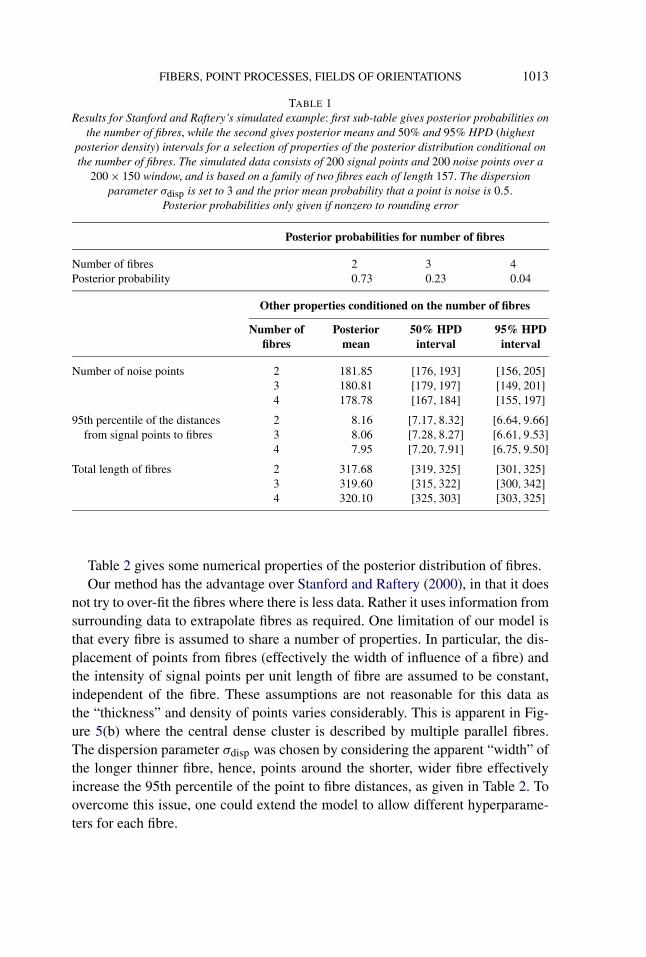
TABLE 1Results for Stanford and Raftery’s simulated example: first sub-table gives posterior probabilities on

the number of fibres, while the second gives posterior means and 50% and 95% HPD (highestposterior density) intervals for a selection of properties of the posterior distribution conditional onthe number of fibres. The simulated data consists of 200 signal points and 200 noise points over a

200 × 150 window, and is based on a family of two fibres each of length 157. The dispersionparameter σdisp is set to 3 and the prior mean probability that a point is noise is 0.5.

Posterior probabilities only given if nonzero to rounding error

Posterior probabilities for number of fibres

Number of fibres 2 3 4Posterior probability 0.73 0.23 0.04

Other properties conditioned on the number of fibres

Number of Posterior 50% HPD 95% HPDfibres mean interval interval

Number of noise points 2 181.85 [176,193] [156,205]3 180.81 [179,197] [149,201]4 178.78 [167,184] [155,197]

95th percentile of the distances 2 8.16 [7.17,8.32] [6.64,9.66]from signal points to fibres 3 8.06 [7.28,8.27] [6.61,9.53]

4 7.95 [7.20,7.91] [6.75,9.50]Total length of fibres 2 317.68 [319,325] [301,325]

3 319.60 [315,322] [300,342]4 320.10 [325,303] [303,325]

Table 2 gives some numerical properties of the posterior distribution of fibres.Our method has the advantage over Stanford and Raftery (2000), in that it does

not try to over-fit the fibres where there is less data. Rather it uses information fromsurrounding data to extrapolate fibres as required. One limitation of our model isthat every fibre is assumed to share a number of properties. In particular, the dis-placement of points from fibres (effectively the width of influence of a fibre) andthe intensity of signal points per unit length of fibre are assumed to be constant,independent of the fibre. These assumptions are not reasonable for this data asthe “thickness” and density of points varies considerably. This is apparent in Fig-ure 5(b) where the central dense cluster is described by multiple parallel fibres.The dispersion parameter σdisp was chosen by considering the apparent “width” ofthe longer thinner fibre, hence, points around the shorter, wider fibre effectivelyincrease the 95th percentile of the point to fibre distances, as given in Table 2. Toovercome this issue, one could extend the model to allow different hyperparame-ters for each fibre.


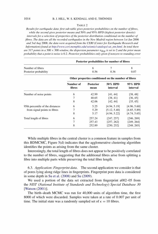
TABLE 2Results for earthquake data: first sub-table gives posterior probabilities on the number of fibres,

while the second gives posterior means and 50% and 95% HPD (highest posterior density)intervals for a selection of properties of the posterior distribution conditional on the number of

fibres. The data are all the recorded earthquakes in the New Madrid region between 1st Jan 2006and 3rd Aug 2008; the data were acquired from the CERI (Center for Earthquake Research and

Information) found at http://www.ceri.memphis.edu/seismic/catalogs/cat_nm.html. In total thereare 317 points in a 300 × 300 window, the dispersion parameter σdisp is set to 2 and the prior meanprobability that a point is noise is 0.2. Posterior probabilities only given if nonzero to rounding error


Number of fibres 6 7 8Posterior probability 0.56 0.36 0.07


Number of Posterior 50% HPD 95% HPDfibres mean interval interval

Number of noise points 6 42.99 [41,44] [38,48]7 40.65 [38,41] [36,45]8 42.06 [42,44] [35,45]

95th percentile of the distances 6 5.25 [4.94,5.19] [4.96,5.60]from signal points to fibres 7 5.29 [5.12,5.40] [4.85,5.89]


7 257.43 [257,262] [249,264]8 252.89 [250,252] [248,265]

While multiple fibres in the central cluster is a common feature in samples fromthis BDMCMC, Figure 5(d) indicates that the agglomerative clustering algorithmidentifies the points as arising from the same cluster.

Interestingly, the total length of fibres does not appear to be positively correlatedto the number of fibres, suggesting that the additional fibres arise from splitting afibre into multiple parts while preserving the total fibre length.

6.3. Application: Fingerprint data. The second application we consider is thatof pores lying along ridge lines in fingerprints. Fingerprint pore data is consideredin some depth in Su et al. (2008) and Su (2009).

We used a portion of the data set extracted from fingerprint a002–05 fromthe NIST (National Institute of Standards and Technology) Special Database 30[Watson (2001)].

The birth–death MCMC was run for 40,000 units of algorithm time, the first8000 of which were discarded. Samples were taken at a rate of 0.007 per unit oftime. The initial state was a randomly sampled set of κ = 10 fibres.

http://www.ceri.memphis.edu/seismic/catalogs/cat_nm.html


(a) (b)

(c) (d)

FIG. 5. New Madrid fault earthquake data. (a) Earthquake data. (b) A random sample from theBDMCMC output. Fibres are represented by curves, pluses indicate points allocated to signal andcrosses indicate points allocated to noise in this sample. (c) Estimate of the density of signal pointsfound by smoothing a series of samples of fibres (darker areas indicate higher densities). Plusesindicate points allocated to signal in at least 50% of samples. The size of points representing thedata has been reduced to enhance the clarity of the density estimate. (d) Estimate of the clustering ofthe signal points—different symbols indicate different clusters, crosses indicate noise. Estimated byconsidering how often pairs of points are associated with the same fibre across a number of samples.

The fingerprint pore data will typically cause breakdown of nearest neighborclustering methods. This is because, while the fibrous structure of the point patternis clear when viewing the global picture, it is not so apparent on a small scale. Thisphenomena is partly due to the apparent inter-ridge alignment of points [from leftto right in Figure 6(a)]. By way of contrast, our field of orientations model takes


(a) (b)

(c) (d)

FIG. 6. Pores from portion of fingerprint a002–05 from the NIST Special Database 30 [Watson(2001)]. (a) Pore data. (b) A random sample from the BDMCMC output. Fibres are represented bycurves, pluses indicate points allocated to signal and crosses indicate points allocated to noise inthis sample. (c) Estimate of the density of signal points found by smoothing a series of samples offibres (darker areas indicate higher densities). The size of points representing the data has beenreduced to enhance the clarity of the density estimate. (d) Estimate of the clustering of the signalpoints—different symbols indicate different clusters, crosses indicate noise. Estimated by consideringhow often pairs of points are associated with the same fibre across a number of samples.

any information available on a small scale and uses it across the window, thanks tothe smoothing step in the field of orientations.

As Figure 6 shows, our model succeeds in fitting many of the fibres (or fin-gerprint ridges) to the pore data. Figure 6(c) indicates areas of doubt in the fibrelocations where the shading is lighter near the edges of the window, showing thatfibre samples were more dispersed.

This data set is an ideal candidate for reconstruction of missing data. We workunder the assumptions that pores lie at fairly regularly intervals along ridges, butsome are not identified during the pore extraction process. Our method uses in-formation from nearby ridges to complete fibres where data is missing. In this


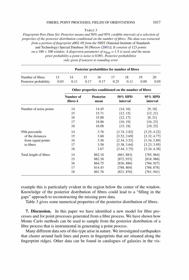
TABLE 3Fingerprint Pore Data Set: Posterior means and 50% and 95% credible intervals of a selection of

properties of the posterior distribution conditional on the number of fibres. The data was extractedfrom a portion of fingerprint a002–05 from the NIST (National Institute of Standards

and Technology) Special Database 30 [Watson (2001)]. It consists of 123 pointson a 100 × 100 window. A dispersion parameter of σdisp = 1.5 is used, and the mean

prior probability a point is noise is 0.091. Posterior probabilitiesonly given if nonzero to rounding error


Number of fibres 13 14 15 16 17 18 19 20Posterior probability 0.03 0.11 0.17 0.17 0.25 0.11 0.09 0.05


Number of Posterior 50% HPD 95% HPDfibres k mean interval interval

Number of noise points 14 14.45 [14,16] [9,18]15 15.71 [12,15] [12,21]16 15.00 [12,17] [8,21]17 18.86 [16,19] [16,23]18 16.08 [15,18] [10,25]

95th percentile 14 3.76 [3.74,3.82] [3.25,4.22]of the distances 15 3.68 [3.52,3.69] [3.32,4.77]from signal points 16 3.56 [2.34,3.52] [3.34,3.89]to fibres 17 3.58 [3.38,3.64] [3.23,3.95]


15 882.38 [872,933] [818,966]16 864.75 [836,886] [784,927]17 814.43 [788,804] [788,878]18 861.76 [821,876] [761,941]

example this is particularly evident in the region below the center of the window.Knowledge of the posterior distribution of fibres could lead to a “filling in thegaps” approach to reconstructing the missing pore data.

Table 3 gives some numerical properties of the posterior distribution of fibres.

7. Discussion. In this paper we have identified a new model for fibre pro-cesses and for point processes generated from a fibre process. We have shown howMonte Carlo methods can be used to sample from the posterior distribution of afibre process that is instrumental in generating a point process.

Many different data sets of this type arise in nature. We investigated earthquakesthat cluster around fault lines and pores in fingerprints that are situated along thefingerprint ridges. Other data can be found in catalogues of galaxies in the vis-


ible universe. Galaxies are known to align themselves along “cosmic” filamentswhich, in turn, connect to form a web-like structure. Understanding these fibresand identifying where they lie is of great interest to cosmologists; see, for exam-ple, Martínez and Saar (2002) for a statistical overview of some current ideas andalso Stoica, Martínez and Saar (2007) for a different approach to modeling the fil-ament structure. Other data sets for which this model may be suitable include thelocations of land mines, often placed in straight lines. Identifying these lines mayaid in the discovery of currently undetected mines. Similar methods of detectingstructure in noisy pictures are a prominent area of research in image recognition.

This process can be used to fit nonparametric curves to point patterns with justtwo limitations on the nature of the curves. The limitations are that the curves mustnot intersect, and that they must be “sufficiently” smooth (i.e., there must be noacute angles in the discretization of the fibres). The smoothness property is desir-able to identify smooth curves rather than complex structures. The nonintersectionproperty may be less desirable but, at some computational cost, the model couldbe generalized to allow each fibre to integrate a different field of orientations.

We do not make use of a deterministic algorithm (such as the EM-algorithm)to fit the fibres, and our approach is not highly sensitive to the choice of startingparameters. Therefore, it can be used to provide interval estimates for various pa-rameters. One of the most sensitive parameters fixed in the algorithm is σ 2

disp whichgoverns the deviation of points from the fibres. If chosen too large, the result willbe too few fibres with a sizeable error in their locations. If chosen too small, fibreclusters may be split into multiple parallel smaller clusters. Our experience is thatthe algorithm is reasonably robust to changes in other parameters.

One strength of our model is that it fits the noise-signal and cluster allocationsimplicitly, in contrast to other cases where the clustering may need to be predeter-mined. The advantage is that we can produce reliability estimates for these clus-tering and noise allocations and explore more potential clustering configurations,and hence more fibre structures.

A limitation of our model arises from the constraints on the similarity of fibres.Fibres are assumed to be of the same width (the displacement of points from thefibres is independent of the fibre), and have the same mean points per unit fibrelength. These are not always reasonable assumptions, as is evidenced by the earth-quake data set. We could extend the model to allow parameters σ 2

disp and η to takedifferent values for each fibre in order to eliminate this issue. A further extensionwould be to include isotropic clusters of points which do not fit well to the “fibre”model.

The complexity of the model, considering the infinite dimensionality of the fieldof orientations, raises the question of whether or not the Markov chain adequatelyexplores the sample space. Our examples indicate that, while the sample space offields of orientations is not explored particularly well, the space of fibre configura-tions is well explored and the field of orientations varies enough to explore a wide


space of fibre configurations. However, as the density of fibres increases, so theMCMC algorithm requires longer runtime in order to overcome these issues.

Note that while our model performs as well as other available techniques on thebasic data sets, it demonstrates significantly better performance on the fingerprintdata where a large number of dense fibre clusters account for most of the data.

It is necessary to bear in mind the ramifications of edge effects in the modeland subsequently the MCMC algorithm. As we are sampling from a bounded sub-set W ⊆ R

2, the omission of potential points just outside W induces a bias ondistance-related measures. The field of orientations will have a bias at the edgefavoring orientations parallel to the sides of a rectangular window W . Fibres arecreated by sampling a random reference point from the field and integrating thefield of orientations from that point. However, the reference point cannot be sam-pled from outside W , and fibres that extend past the boundary of W are typicallyterminated on the border as no field of orientations is available past that point.Also, the model for the displacement of points from fibres does not account foredge effects. Most of these algorithmic biases would be significantly decreasedby creating a border around W and completing the analysis over the whole area.However, this would come at an additional computational cost.

We have commented in passing on the phenomenon of curvature bias and its ef-fects on the estimation of parameters, and we note this as a fruitful area for futureresearch. Further research possibilities include the fitting of two-dimensional sur-faces in 3 dimensions. Then new geometric issues need to be taken into account;for example, it is not the case that a generic field of tangent planes can be devel-oped into a fibration by surfaces. It is hoped to investigate this problem in furtherwork.

REFERENCES

ADLER, R. J. and TAYLOR, J. E. (2007). Random Fields and Geometry. Springer, New York.MR2319516

ARSIGNY, V., FILLARD, P., PENNEC, X. and AYACHE, N. (2006). Log-Euclidean metrics for fastand simple calculus on diffusion tensors. Magn. Reson. Med. 56 411–421.

AUGUST, J. and ZUCKER, S. W. (2003). Sketches with curvature: The curve indicator random fieldand Markov processes. IEEE Trans. Pattern Anal. Mach. Intell. 25 387–400.

BARROW, J. D., BHAVSAR, S. P. and SONODA, D. H. (1985). Minimal spanning trees, filamentsand galaxy clustering. Royal Astronomical Society, Monthly Notices 216 17–35.

BROOKS, S. P. and ROBERTS, G. O. (1998). Convergence assessment techniques for Markov chainMonte Carlo. Statist. Comput. 8 319–335.

DRYDEN, I. L., KOLOYDENKO, A. and ZHOU, D. (2009). Non-Euclidean statistics for covari-ance matrices, with applications to diffusion tensor imaging. Ann. Appl. Stat. 3 1102–1123.MR2750388

GENOVESE, C. R., PERONE-PACIFICO, M., VERDINELLI, I. and WASSERMAN, L. (2009). On thepath density of a gradient field. Ann. Statist. 37 3236–3271.

HILL, B. J. (2011). An orientation field approach to modelling fibre-generated spatial point pro-cesses. Ph.D. thesis, Univ. Warwick. Available at http://www2.warwick.ac.uk/go/ethonnes/fibres/Hill.pdf.

http://www.ams.org/mathscinet-getitem?mr=2319516


http://www2.warwick.ac.uk/go/ethonnes/fibres/Hill.pdf

http://www2.warwick.ac.uk/go/ethonnes/fibres/Hill.pdf


ILLIAN, J., PENTTINEN, A., STOYAN, H. and STOYAN, D. (2008). Statistical Analysis and Mod-elling of Spatial Point Patterns. Wiley, New York.

KASPI, H. and MANDELBAUM, A. (1994). On Harris recurrence in continuous time. Math. Oper.Res. 19 211–222. MR1290020

LE BIHAN, D. L., MANGIN, J. F., POUPON, C., CLARK, C. A., PAPPATA, S., MOLKO, N. andCHABRIAT, H. (2001). Diffusion tensor imaging: Concepts and applications. J. Magn. Reson.Imaging 13 534–546.

LI, C., SUN, X., ZOU, K., YANG, H., HUANG, X., WANG, Y., LUI, S., LI, D., ZOU, L. andCHEN, H. (2007). Voxel based analysis of DTI in depression patients. International Journal ofMagnetic Resonance Imaging 1 43–48.

MARTÍNEZ, V. J. and SAAR, E. (2002). Statistics of the Galaxy Distribution. Chapman & Hall/CRC,Boca Raton, FL.

MØLLER, J. and WAAGEPETERSEN, R. P. (2004). Statistical Inference and Simulation for SpatialPoint Processes. Monographs on Statistics and Applied Probability 100. Chapman & Hall, Lon-don. MR2004226

PEARL, J. (1988). Probabilistic Reasoning in Intelligent Systems: Networks of Plausible Inference.Morgan Kaufmann, San Mateo. MR0965765

STANFORD, D. C. and RAFTERY, A. E. (2000). Finding curvilinear features in spatial point pat-terns: Principal curve clustering with noise. IEEE Transactions on Pattern Analysis and MachineIntelligence 22 601–609.

STOICA, R. S., MARTÍNEZ, V. J. and SAAR, E. (2007). A three-dimensional object point processfor detection of cosmic filaments. Appl. Statist. 56 459–477.

STOICA, R. S., MARTÍNEZ, V. J. and SAAR, E. (2010). Filaments in observed and mock galaxycatalogues. Astronomy and Astrophysics 510 1–12.

STOICA, R. S., MARTÍNEZ, V. J., MATEU, J. and SAAR, E. (2005). Detection of cosmic filamentsusing the Candy model. Astronomy and Astrophysics 434 423.

STOYAN, D., KENDALL, W. S. and MECKE, J. (1995). Stochastic Geometry and Its Applications,2nd ed. Wiley, New York.

SU, J. (2009). A tensor approach to fingerprint analysis. Ph.D. thesis, Univ. Warwick.SU, J., HILL, B. J., KENDALL, W. S. and THÖNNES, E. (2008). Inference for point processes with

unobserved one-dimensional reference structure. CRiSM Working Paper 8-10, Univ. Warwick.WATSON, C. (2001). NIST special database 30: Dual resolution images from paired fingerprint cards.

National Institute of Standards and Technology, Gaithersburg.

DEPARTMENT OF STATISTICS

UNIVERSITY OF WARWICK

COVENTRY, CV4 7ALUNITED KINGDOM

E-MAIL: [email protected]@[email protected]




mailto:[email protected]



fibre-generated point processes and fields of orientations

Documents