field examples of the combined petrophysical inversion of ... · field examples of the combined...

SPWLA 50th Annual Logging Symposium, June 21-24, 2009

1

FIELD EXAMPLES OF THE COMBINED PETROPHYSICAL INVERSION OF GAMMA-RAY, DENSITY, AND RESISTIVITY LOGS ACQUIRED IN THINLY-BEDDED CLASTIC ROCK FORMATIONS

Jorge A. Sanchez-Ramirez, Carlos Torres-Verdín, Gong Li Wang, Alberto Mendoza, David

Wolf, and Zhipeng Liu, The University of Texas at Austin, and Gabriela Schell, BHP Billiton

Copyright 2009, held jointly by the Society of Petrophysicists and Well Log Analysts (SPWLA) and the submitting authors. This paper was prepared for presentation at the SPWLA 50th Annual Logging Symposium held in The Woodlands, Texas, United States, June 21-24, 2009.

ABSTRACT Limited vertical resolution of logging tools causes shoulder-bed effects on borehole measurements, there-fore biases in the assessment of porosity and hydrocar-bon saturation across thinly-bedded rock formations. Previously, we developed a combined inversion proce-dure for induction resistivity and density logs to im-prove the petrophysical assessment of multi-layer res-ervoirs. In this paper, we include the inversion of gamma-ray (GR) logs in the interpretation method and evaluate three field cases that comprise hydrocarbon-saturated Tertiary turbidite sequences. Formations un-der consideration are unconsolidated to poorly consoli-dated. All wells were drilled with oil-base mud (OBM), logged with triple-combo tools, and sampled with whole and sidewall cores. We transform layer-by-layer inversion results into petrophysical properties via a shaly-sand model. On average, inversion results yield 19% better agreement to core measurements and lead to 28% increase in hy-drocarbon reserves when compared to standard well-log interpretation procedures. The wide variety of sand-shale distributions and layer thicknesses included in the example data sets en-ables us to generalize recommendations for best prac-tices of combined inversion, including criteria for bed-boundary detection, sensor selection, and modification of our “UT Longhorn Tool” flux sensitivity functions (FSFs) to replicate those of commercial tools. The most critical step for reliable and accurate inversion results is the detection/selection of bed boundaries. Inversion of field data also indicates that the minimum bed thickness resolvable with combined inversion is about 0.7ft, and that inflection points of density logs are the best option for bed-boundary detection. We show that combined inversion allows the detec-tion of noisy, inconsistent, and inadequate measure-ments, including cases of abnormal measurement-correction biases otherwise difficult to diagnose on processed logs.

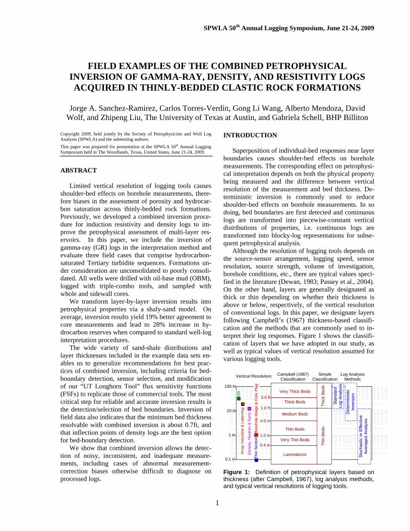
INTRODUCTION Superposition of individual-bed responses near layer boundaries causes shoulder-bed effects on borehole measurements. The corresponding effect on petrophysi-cal interpretation depends on both the physical property being measured and the difference between vertical resolution of the measurement and bed thickness. De-terministic inversion is commonly used to reduce shoulder-bed effects on borehole measurements. In so doing, bed boundaries are first detected and continuous logs are transformed into piecewise-constant vertical distributions of properties, i.e. continuous logs are transformed into blocky-log representations for subse-quent petrophysical analysis. Although the resolution of logging tools depends on the source-sensor arrangement, logging speed, sensor resolution, source strength, volume of investigation, borehole conditions, etc., there are typical values speci-fied in the literature (Dewan, 1983; Passey et al., 2004). On the other hand, layers are generally designated as thick or thin depending on whether their thickness is above or below, respectively, of the vertical resolution of conventional logs. In this paper, we designate layers following Campbell’s (1967) thickness-based classifi-cation and the methods that are commonly used to in-terpret their log responses. Figure 1 shows the classifi-cation of layers that we have adopted in our study, as well as typical values of vertical resolution assumed for various logging tools.

Very Thick Beds

Thin Beds

Laminations

SS tt aa

nn ddaa rr

dd LL oo

gg AA n

n aall yy

ss iiss

Medium Beds

Thick Beds

0.1 in

1 in

10 in

100 in

BBoo rr

ee hhoo ll

ee II mm

aa ggee

&& CC

oo rree

PP ll uu

gg TT hh

ii nn SS

ee cctt ii oo

nn

DDee nn

ss iitt yy

,, NNee uu

tt rr oonn

&& SS

oo nnii cc

AArr rr

aa yy II nn

dd uucc tt

ii oonn

&& LL

aa ttee rr

oo lloo gg

GG

RR

DDee tt

ee rrmm

ii nnii ss

tt ii cc

II nnvv ee

rr ssii oo

nn

SStt oo

cc hhaa ss

tt ii cc oo

rr EEff ff ee

cc ttii vv

ee AA v

v eerr aa

gg eedd

AAnn aa

ll yyss ii

ss

Very Thin Beds 0.4 in Th

in B

eds

Thic

k Be

ds

Vertical Resolution Campbell (1967) Classification

Simple Classification

Log Analysis Methods

1.0 in

4.0 in

1.0 ft

3.0 ft

Figure 1: Definition of petrophysical layers based on thickness (after Campbell, 1967), log analysis methods, and typical vertical resolutions of logging tools.


2

Shoulder-bed effects in very thick layers are re-garded negligible because in those cases the vertical resolution of the measurements is shorter than the thickness of the layers; i.e. well logs have the resolution necessary to resolve true layer petrophysical properties, hence standard log analysis is deemed accurate to esti-mate hydrocarbon reserves. The thickness of thick and medium beds is compa-rable to the vertical resolution of most conventional well logs, whereby logs can be adversely affected by shoulder beds to the point of rendering standard log analysis unreliable. Deterministic inversion can be used to reduce shoulder-bed effects and improve the estima-tion of true physical and petrophysical properties of multi-layer sequences. Conventional well logs cannot resolve thin beds, very thin beds, and laminations because bed thickness is too small when compared to the vertical resolution of logs. Across this type of layers, conventional logs re-spond to effective-medium properties, average petro-physical properties and net-to-gross, and do not lend themselves to the detection of individual bed bounda-ries. Without bed boundaries, it is not possible to define multi-layer models. Even if bed boundaries were de-tected from other measurements (e.g. high-resolution logs, borehole images, or core data), deterministic in-version would be rendered highly non-unique, thereby leading to unstable and inaccurate results. Different deterministic inversion techniques are commonly used to interpret measurements acquired across thin beds, very thin beds, and laminations. The two most common approaches are (a) stochastic inver-sion to estimate global statistical properties of sedimen-tary units, and (b) calculation of effective properties via Thomas-Stieber’s approach (Thomas et al., 1975), or by incorporating advanced measurements in the interpreta-tion method such as NMR, multi-component resistivity, and borehole images. Deterministic inversion has been previously used to refine petrophysical interpretations across thin beds. Fast inversion methods, in particular, have enabled practical field applications over long depth sections of logs. Wang et al. (2009), Zhang et al. (1995), and Zhang et al. (1999) proposed simulation and inversion methods for quick interpretation of array-induction re-sistivity (AIT1) measurements. Mendoza et al. (2007) developed a fast method to simulate density, neutron and GR logs based on linear weighting functions (FSFs, or Flux Scattering Functions) calculated with Monte Carlo simulations of particle-level transport in homoge-nous media. Liu et al. (2007) developed a method for combined inversion of density and resistivity logs based on Mendoza et al.’s (2007) fast linear simulation

1 Mark of Schlumberger.

method and Wang et al.’s (2009) fast nonlinear inver-sion methods. The combined inversion developed in this paper is an extension of Liu et al.’s (2007) joint inversion method for density and resistivity logs in which we have all also included GR logs as input data. Inversion of GR logs is necessary because of their low vertical resolution compared to density and resistivity logs, and because of the importance of GR logs in the calculation of volumetric concentration of shale, Csh. Previously published projects on well-log inversion do not report examples of application to field measure-ments. Examples are limited to either relatively simple field cases or synthetic models. The main objective of this paper is to test the combined inversion approach on challenging field examples that include core data for cross-validation of results. In addition, we seek to com-pile a set of best practices for the routine application of combined inversion of field logs. The field cases analyzed in this paper correspond to turbidite sedimentary sequences in the deepwater Gulf of Mexico. Layer thicknesses range from thin lamina-tions to very thick beds. This wide range of thickness variations prompts us to divide the field applications of combined inversion into two groups: (a) cases of com-bined inversion for medium, thick, and very thick lay-ers, and (b) cases of laminar models for thin beds and laminations. In this paper, we focus our attention to the first group of applications. Sanchez-Ramirez (2009) describes examples of combined inversion for the sec-ond group of applications. METHOD The inversion method assumes a vertical wellbore penetrating a stack of horizontal layers, as well as axi-ally symmetric mud-filtrate invasion. Moreover, we assume layer-by-layer isotropic electrical resistivity. Combined inversion consists of four main sequential steps: (a) detection of bed boundaries, (b) separate in-version of density, GR, and resistivity logs, (c) forward simulation of inverted layer properties to calculate data misfits, and (d) calculation of petrophysical properties from inversion results. Bed Boundary Selection Bed boundaries are detected based on inflection points of a master log. In turn, inflection points are de-termined by calculating the variance of the master log within a sliding depth window, and by placing a bed boundary wherever the variance increases above a pre-specified threshold. Forward Simulation and Inversion After bed-boundary selection, we perform separate inversion of each measurement based on available raw


3

data (mono-sensor data for density, standard resolution GR, and single-array borehole-corrected conductivity measurements for induction resistivity) to calculate layer-by-layer density, GR, and resistivity. The inversion of density and GR logs is based on Mendoza et al.’s (2007) rapid linear iterative refinement simulation method for borehole nuclear measurements using approximate FSFs constructed for general density and GR tools (UT Longhorn Tools). The FSFs are aver-aged radially (one-dimensional, 1D FSF) for their im-plementation to invert density and GR logs into layer-by-layer values of bulk density and total GR. Inversion of AIT induction resistivity measurements is performed with a fast nonlinear minimization proce-dure developed by Wang et al. (2009). Inputs to this inversion are raw sub-array resistivity measurements; outputs are layer-by-layer values of invaded-zone resis-tivity (Rxo), true resistivity (Rt), and radial length of mud-filtrate invasion.

Deterministic inversion can be formulated as the minimization of the quadratic cost function

( ) ( ){ }2 220

12

C λ= + −x e x x x , (1)

where x is a vector containing the unknown layer properties, ( )xe is the vector of data misfits or data residuals, and λ is a stabilization parameter that re-quires that the solution ( x ) to be close to certain prior,

0x (Hansen, P. C., 1998). The stabilization (regulariza-tion) additive term in the cost function is necessary to reduce instability in the solution due to noisy and in-adequate measurements. In our case, 0x is equal to a representative reading of well logs within the inverted depth interval, which can be the average, minimum, or maximum value depending on the behavior of well logs. The vector of data residuals is written as

( ) ( ) 0dxdxe −= , (2)

where )(xd is the vector of numerically simulated log

values, and 0d is the vector of field measurements. Data misfits quantify and verify the consistency of in-verted results with available measurements. For GR and density log inversion, we assume linear-ity between measurements and layer properties, where-upon numerically simulated logs are given by

( ) xFSFxd ⋅= , (3)

where the matrix FSF is constructed with 1D (radially averaged) FSFs. Substitution of equation (3) into (1) yields

( )20 22

012

C λ⎧ ⎫= ⋅ − + −⎨ ⎬⎩ ⎭

x FSF x d x x , (4)

which we minimize using Tikhonov et al.’s (1977) regularization method. On the other hand, inversion of induction resistivity measurements into layer-by-layer resistivity values re-quires nonlinear minimization. Accordingly, we ap-proach the minimization of resistivity measurements with linear iterative steps via the Gauss-Newton method together with an efficient approximation of Fréchet derivatives (Wang et al., 2009). Petrophysical Interpretation After completing the three separate inversions, re-sults are combined using a shaly-sand model (i.e. Waxman-Smits, Juhasz, Dual-Water, etc.) to calculate layer-by-layer porosity and saturation. The latter calcu-lations are subsequently compared to basic log interpre-tation using the same shaly-sand model and associated parameters (a, m, n, Rw, etc.) For example, Best et. al’s (1980) Dual-Water equa-tion is given by

⎥⎥⎦

⎤

⎢⎢⎣

⎡⎟⎟⎠

⎞⎜⎜⎝

⎛−+⋅=

wwbwt

wb

w

nwt

mt

t RRSS

RaS

R1111 φ , (5)

where Rt is true formation resistivity, φt is total poros-ity, Swt is total water saturation, Swb is bound-water satu-ration, Rw is connate water resistivity, Rwb is bound-water resistivity, a is the tortuosity factor, and m and n are the cementation (lithology) and saturation expo-nents, respectively. Non-shale porosity (φs) is calculated using the den-sity composition equation for a unit rock volume, given by

( )( )[ ] swshwsw

sshmshshr

SSCC

φρρφρρρ

−++−−+=

1 1

, (6)

where ρr is bulk rock density, ρsh is density of wet shale, ρm is density of matrix, ρw is density of water, ρh is density of hydrocarbon, Csh is volumetric concentra-tion of wet shale, and Sws is non-shale water saturation. It follows that

( )( ) mwshwsw

shmshshrs SS

CCρρρ

ρρρφ−−+−−−

=1

1 . (7)

The expressions used to calculate Sws, Swb and φt are given by

wb

wbwtws S

SSS−−

=1

, (8)

shshs

shshwb C

CSφφ

φ+

= , (9)

and shshst C φφφ += , (10)


4

where φsh is total porosity of wet shale. Volumetric concentration of wet shale (Csh) is calculated using a linear shale index, given by

ssh

ssh GRGR

GRGRC−−

= , (11)

where GR is total gamma-ray reading, GRs is gamma-ray reading in clean sands, and GRsh is gamma-ray reading in shales. Hydrocarbon pore-volume (HPV) and net-to-gross ratio (NGR) are calculated with the algorithm

( ) ,1

1ay elseif 0aythen

,or , , if

1∑=

−−−

⋅Δ⋅−⋅=

==

><>

n

iiiwss

ii

cfwswscfsscfshsh

payhSHPV

pp

SSCC

ii

iii

φ

φφ

, 1

i

n

iii hpayhNGR Δ⎟⎟⎠

⎞⎜⎜⎝

⎛⋅Δ= ∑

= (12)

where Δhi is vertical depth increment, Csh-cf is cutoff for Csh, φs-cf is cutoff for φs, Sws-cf is cutoff for Sws, and payi is a flag to differentiate pay from non pay.

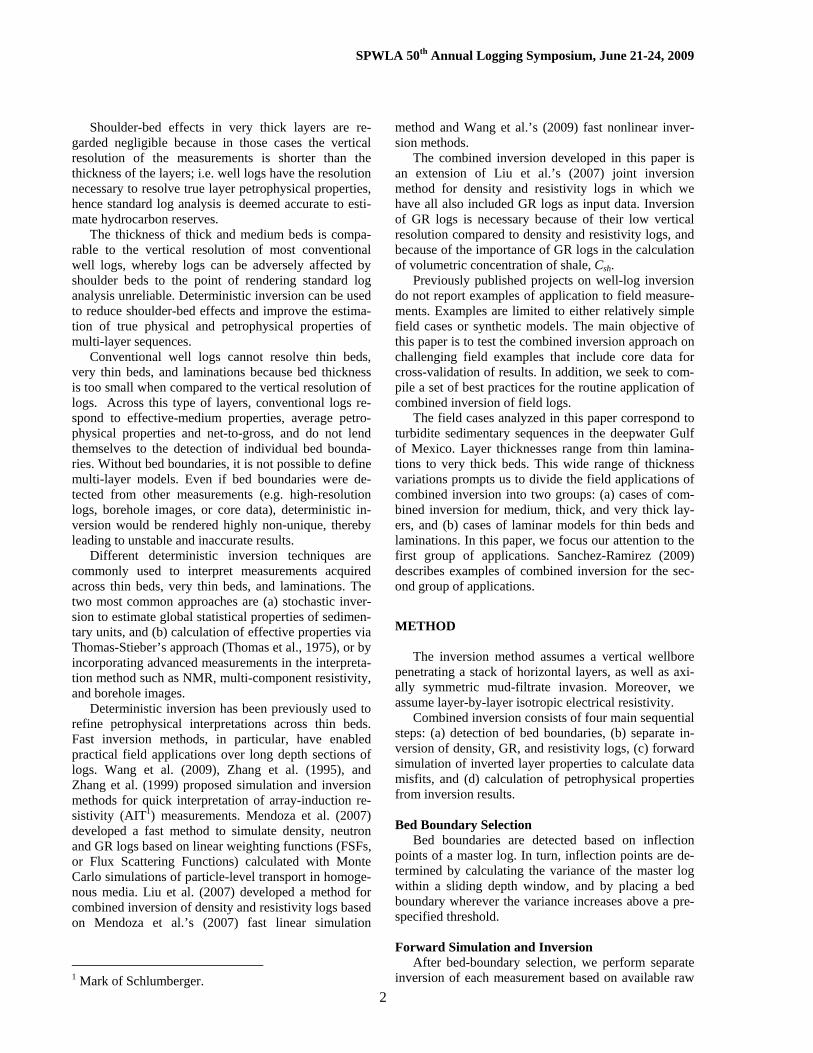
Figure 2: Example of a Permian channel margin in the Laingsburg area, Karoo, South Africa (photograph by Ian Westlake, BHP Billiton).

SEM photo at 10.6ft

Csh=15% at 11.0ft

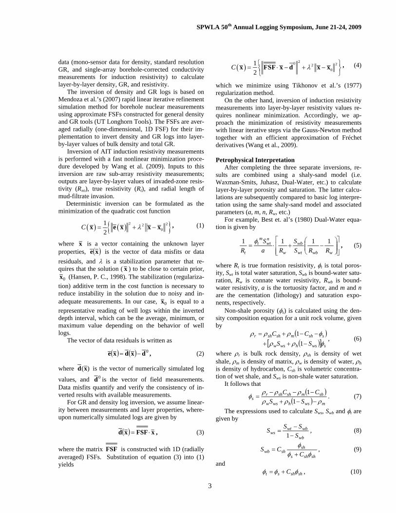
Figure 3: Ultraviolet and normal-light photograph of core retrieved in Well No. 3 between 10.5 ft and 11.5 ft. The scanning electron microscope (SEM) photograph indicates pore-bridging illite at 10.6 ft. Laser-grain tests measured Csh=15% at 11.0 ft.

FIELD CASES OF COMBINED INVERSION We implemented the combined inversion of density, GR, and induction resistivity logs with data acquired in three wells within three different fields located in the deepwater Gulf of Mexico. Formations under consid-eration are unconsolidated to poorly consolidated shaly-sand sequences in turbidites depositional systems. Sedimentary units are channelized sand-sheet systems anywhere from mid-slope to basin-floor positions. Figure 2 shows the outcrop of a turbidite channel mar-gin where the distribution and thickness of sand-shale layers is similar to that of the field examples discussed in this section. Depth segments chosen for inversion are sequences of oil-bearing sands and shale layers. Whole and side-wall core samples were recovered for cross-verification of measurements and interpretations. We converted inversion results to layer-by-layer petrophysical properties using the Dual-Water model with the parameters listed in Table 1. A dispersed-shaly-sand model such as Dual-Water is necessary for interpretation because of evidence of dispersed clay in sand units. For example, volumetric shale concentration measured with laser grain tests (LGTs) for Wells Nos. 2 and 3 in sandy medium and thick beds exhibits varia-tions from 3% to 30%, and up to 70% in thin beds and laminations. Figure 3 shows an example of illite coat-ing the surface of quartz grains in Well No. 3 at 10.6ft. Alternatively, Well No. 1 could have been analyzed with Archie’s equation because sand units are relatively clean (Csh less than 20%). Invasion was not considered in the interpretation of field cases because of the lack of measurable contrast between deep- and shallow-sensing apparent resistivi-ties. This lack of radial resistivity contrast is due to the absence of free water and presence of OBM in the sand units under study. Table 2 shows NGR and HPV calculations for the analyzed wells using four sets of logs for GR, bulk rock density (ρr), and true resistivity (Rt). The sets of logs comprise standard resolution (SR) logs (SR SR SR), high resolution (HR) logs (HR HR HR), SR GR with layer-by-layer density and resistivity estimated from separate inversion (SR SI SI), and combined results from separate inversions (SI SI SI). Table 3 describes the agreement of interpretation results with core meas-urements in terms of linear correlation coefficients (R2) and relative error (RE) using the same four sets of well logs mentioned above. Tables 4 and 5 describe the per-cent changes of (a) hydrocarbon reserves calculations and (b) agreement with core data, respectively, with respect to SR results (SR SR SR).


5

Well No. 1 The analyzed depth interval is composed of three sand units separated by heterolithic, mud rich shaly intervals logged with CNT-LDT-SGT-AIT2, CMR-GR2 and OBMI-GR2. Core measurements indicate that the three sand units exhibit similar petrophysical properties; however, their log responses are different. Log differ-ences are due to shoulder-bed effects because the

Table 1: Summary of petrophysical parameters as-sumed for the Dual-Water petrophysical interpretation of Wells No.1, 2 and 3.

Well No. Property Unit 1 2 3 Petrophysical Parameters

Sw-φ Model - DualW. DualW. DualW. GRs GAPI 18 20 25 GRsh GAPI 83 95 125 Csh model - Linear Linear Linear a - 1.0 1.0 1.0 m - 1.8 1.80 1.80 n - 2.1 2.00 1.71 Rw Ohm-m 0.05 0.05 0.04 Rwb Ohm-m 0.06 0.06 0.035 φsh p.u. 0.16 0.18 0.12 ρm gr/cc 2.65 2.65 2.65 ρw gr/cc 1.00 1.00 1.00 ρh gr/cc 0.852 0.852 0.800 ρsh gr/cc 2.42 2.45 2.536

Cutoffs for Reserves Calculations Sws-cf - 0.65 0.65 0.65 φs-cf - 0.15 0.15 0.15 Csh-cf - 0.4 0.4 0.4

Inversion-Related Parameters LS3 used - Yes Yes Yes SS4 used - No No No LS FSF factor - 1.25 1.1 1.1 GR FSF factor - 2.10 2.01 2.10 Regularization GR - No No No Regularization Den. - No No No AIT filtrate invasion - No No No AIT sub-arrays - 2 to 8 2 to 6 3 to 8 AIT type - B H H AIT lower window - 8 8 8 AIT central window - 6 6 6 AIT upper window - 8 8 8 AIT noise level - 0.0 0.0 0.0 AIT iterations - 100 100 100 AIT regular. factor - 10 10 10

2 Marks of Schlumberger. 3 LS stands for long spacing density. 4 SS stands for long spacing density.

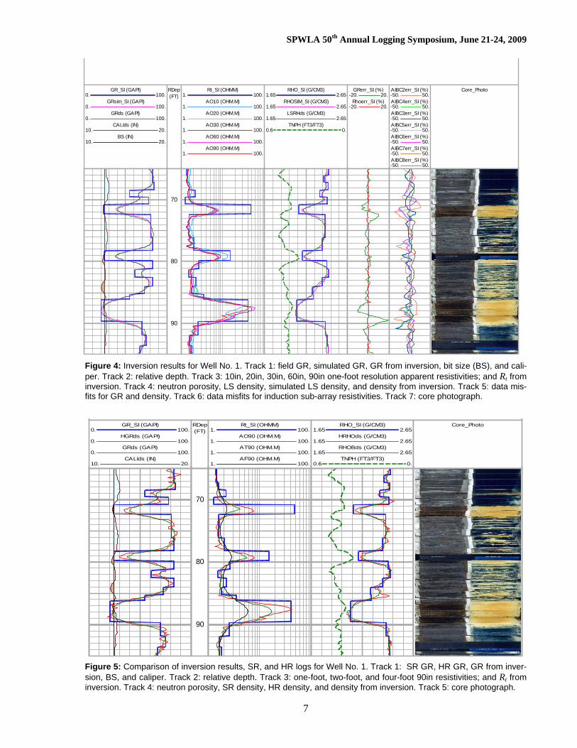
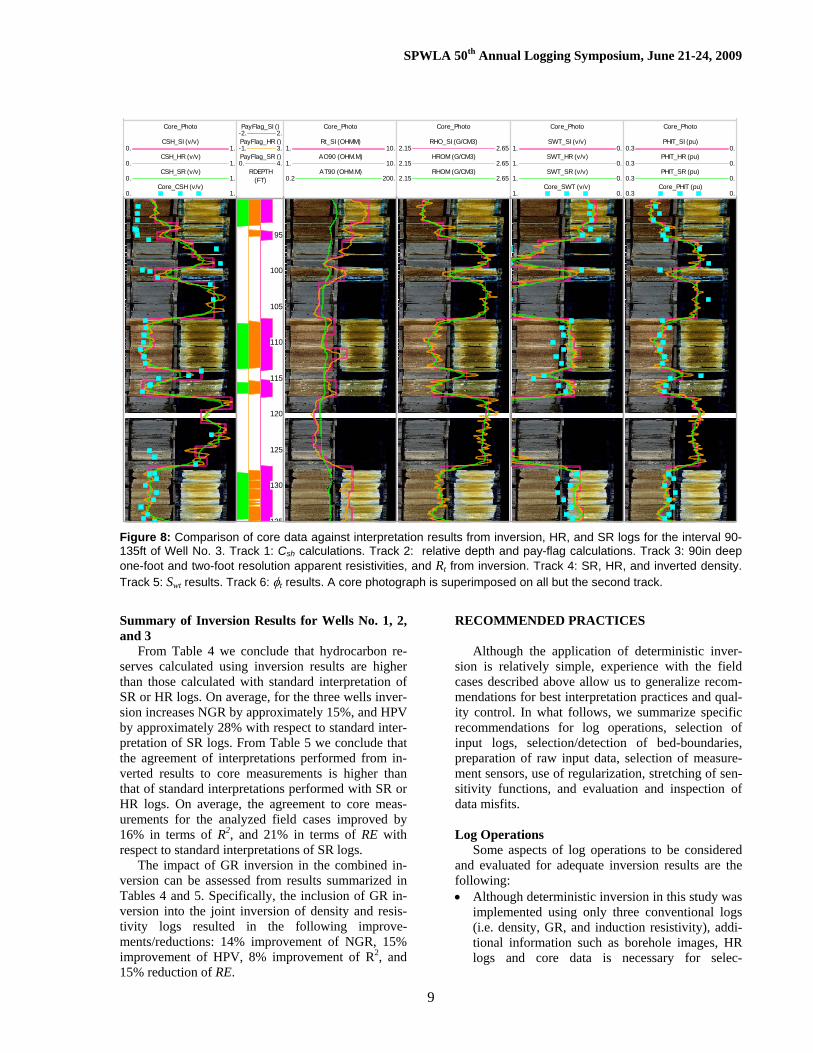
sand units represent thick beds with thicknesses (1.75ft, 1.7ft and 3.8ft) comparable to the vertical resolution of logging tools. Figure 4 shows the corresponding inversion results and data misfits for this case. Well logs barely resolve the thicker lower sand unit but cannot resolve the petrophysical properties of the thinner upper layers. Figure 5 indicates that HR measurements are closer to the inverted results than SR logs. Figure 6 shows core data, as well as Csh, Sws, Swt, φs and φt calculated from both standard resolution meas-urements and inverted results using the Dual-Water model with the properties listed in Table 1. This figure indicates that interpretations from inverted results agree better with core measurements than those obtained from standard well-log interpretation using SR logs. Table 5 quantifies the corresponding percent improvement with respect to standard well-log interpretation as 5% on average for R2 and 38% as the average reduction for RE. In the laminated sections of the well (e.g. 72.5ft to 78ft), logs measure effective shale- and sand-layer properties, whereas bed boundaries cannot be detected from inflection points of logs. Moreover, if bed bounda-ries were selected from a borehole image or core data, deterministic inversion would be rendered highly non-unique (hence unstable). Parenthetically, we performed the same analysis on well logs acquired in a side track of Well No. 1 obtain-ing practically equivalent results. However, core data were not available in that well and therefore results are not reported here. Well No. 2 The thickness of the analyzed section is 150ft, which is composed of amalgamated and non-amalgamated sheet sands on top of heterolithic shaly sands. The formation was logged with PEX-AIT-CMR2 and OBMI-DSI-GR2. Figure 7 compares inversion re-sults to core measurements. From Table 5, we observe that the percent match to core measurements improved 30% for R2 and 17% for RE relative to standard well-log interpretation. Likewise, HPV calculations in-creased by approximately 9% when inversion results were used in the interpretation (see Table 4). Well No. 3 The thickness of the analyzed section is 260ft. It consists of amalgamated and non-amalgamated sheet sands intercalated with heterolithic shaly sands that were logged with HAPS-HLDS-QAIT-SGT2. Inversion results improve the agreement with core measurements (15% in terms of R2 and 9% in terms of RE) compared to results from standard well-log interpretation.


6

Table 2: Summary of calculated hydrocarbon re-serves using inverted results, SR, and HR logs.

Type of Logs Used5 Well No. GR ρr Rt 1 2 3

NGR (frac.) SR SR SR 0.110 0.355 0.349 HR HR HR 0.124 0.346 0.371 SR SI SI 0.108 0.348 0.369 SI SI SI 0.135 0.364 0.418

HPV (hydrocarbon-ft) SR SR SR 1.12 10.79 9.72 HR HR HR 1.35 10.97 10.43 SR SI SI 1.41 11.27 10.53 SI SI SI 1.73 11.77 11.65

Table 3: Summary of calculated correlation betweencore measurements and calculations from inverted results, SR, and HR logs.

Type of Logs Used Well No. GR ρr Rt 1 2 3

SR SR SR 0.708 0.761 0.413 HR HR HR 0.696 0.782 0.419 SR SI SI 0.709 0.763 0.411 R

2

SI SI SI 0.765 0.804 0.457 SR SR SR 143.0 68.1 68.4 HR HR HR 134.0 70.0 66.5 SR SI SI 143.0 67.9 68.4

Csh

RE

%

SI SI SI 47.1 58.1 61.6 SR SR SR 0.565 0.304 0.473 HR HR HR 0.579 0.273 0.424 SR SI SI 0.580 0.365 0.531 R

2


φ t

RE

%

SI SI SI 23.0 10.2 11.4 SR SR SR 0.675 0.583 0.243 HR HR HR 0.698 0.749 0.202 SR SI SI 0.658 0.701 0.296 R

2


S wt

RE

%

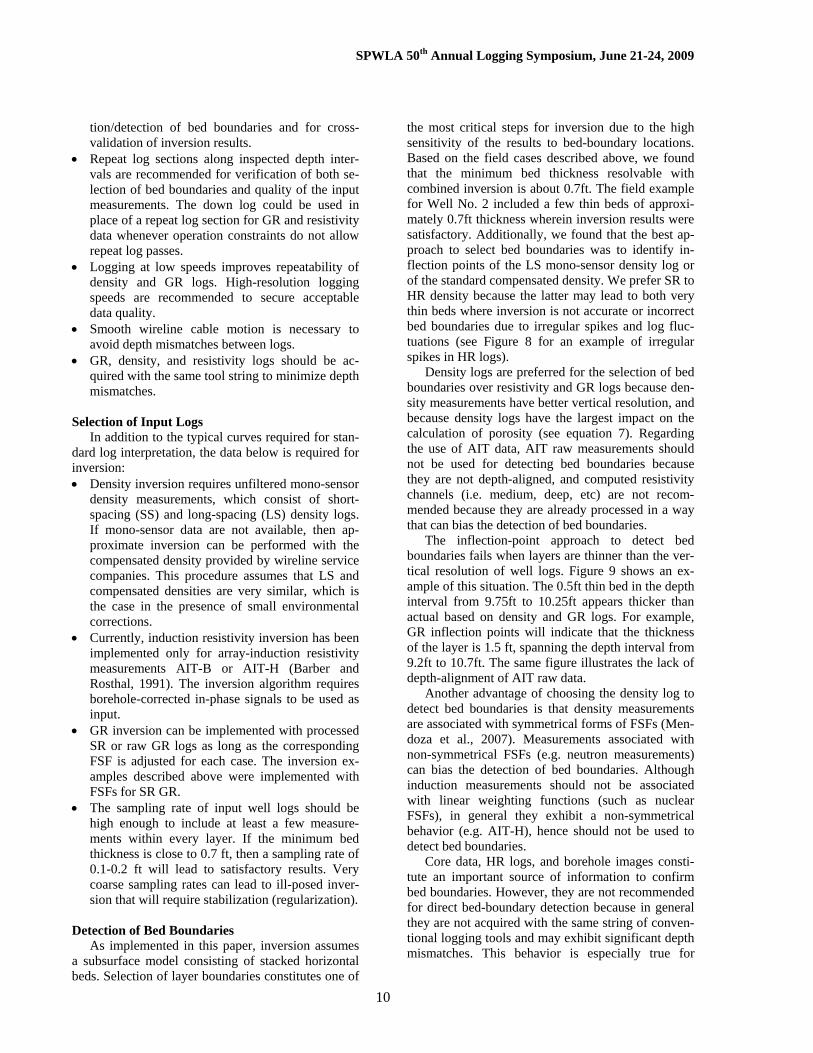
SI SI SI 58.0 38.2 32.8 Figure 8 is a close-up view of one of the core sections together with inversion results. The sharpening of lay-ers that results from inversion is very close to that of bed boundaries observed in the core photograph, whereby the pay flag calculated from inversion results is higher than the one calculated from standard well-log interpretation in this well.

5 SR stands for standard resolution, HR for high resolu-tion, and SI for separate inversion.

Table 4: Percent changes of reserves calculations with respect to SR calculations.

Type of Logs Used Well No. GR ρr Rt 1 2 3 Aver

NGR Change Respect SR Logs (%) SR SR SR - - - - HR HR HR 12.7 -2.5 6.3 5.5 SR SI SI -1.8 -2.0 5.7 0.6 SI SI SI 22.7 2.5 19.8 15.0

HPV Change Respect SR Logs (%) SR SR SR - - - - HR HR HR 20.5 1.7 7.3 9.8 SR SI SI 25.9 4.4 8.3 12.9 SI SI SI 54.5 9.1 19.9 27.8

Table 5: Percent changes of correlations between core measurements and interpretation results with respectto SR results.

Type of Logs Used Well No. GR ρr Rt 1 2 3 Aver

SR SR SR - - - - HR HR HR -1.7 2.8 1.5 0.8 SR SI SI 0.1 0.3 -0.5 0.0 R

2

SI SI SI 8.1 5.7 10.7 8.1 SR SR SR - - - - HR HR HR -6.3 2.8 -2.8 -2.1 SR SI SI 0.0 -0.3 0.0 -0.1

Csh

RE

%

SI SI SI -67.1 -14.7 -9.9 -30.6 SR SR SR - - - - HR HR HR 2.5 -10.2 -10.4 -6.0 SR SI SI 2.7 20.1 12.3 11.7 R

2

SI SI SI -0.4 49.7 15.9 21.7 SR SR SR - - - - HR HR HR 0.9 22.3 17.3 13.5 SR SI SI 10.4 2.9 -7.1 2.1

φ t

RE

%

SI SI SI 0.0 -1.0 -10.2 -3.7 SR SR SR - - - - HR HR HR 3.4 28.5 -16.9 5.0 SR SI SI -2.5 20.2 21.8 13.2 R

2

SI SI SI 7.1 33.4 17.7 19.4 SR SR SR - - - - HR HR HR -19.0 1.5 5.1 -4.1 SR SI SI -30.4 -31.3 -6.3 -22.7

S wt

RE

%

SI SI SI -48.2 -34.7 -6.8 -29.9 Average

SR SR SR - - - - HR HR HR 1.4 7.0 -8.6 -0.1 SR SI SI 0.1 13.5 11.2 8.3 R

2

SI SI SI 4.9 29.6 14.7 16.4 SR SR SR - - - - HR HR HR -8.1 8.9 6.6 2.4 SR SI SI -6.7 -9.6 -4.4 -6.9

Ave

rage

RE

%

SI SI SI -38.4 -16.8 -9.0 -21.4


7

GR_SI (GAPI)0. 100.

GRsim_SI (GAPI)0. 100.

GRds (GAPI)0. 100.

CALIds (IN)10. 20.

BS (IN)10. 20.

RDep(FT)

Rt_SI (OHMM)1. 100.

AO10 (OHM.M)1. 100.

AO20 (OHM.M)1. 100.

AO30 (OHM.M)1. 100.

AO60 (OHM.M)1. 100.

AO90 (OHM.M)1. 100.

RHO_SI (G/CM3)1.65 2.65

RHOSIM_SI (G/CM3)1.65 2.65

LSRHds (G/CM3)1.65 2.65

TNPH (FT3/FT3)0.6 0.

GRerr_SI (%)-20. 20.

Rhoerr_SI (%)-20. 20.

AIBC2err_SI (%)-50. 50.AIBC4err_SI (%)-50. 50.AIBC3err_SI (%)-50. 50.AIBC5err_SI (%)-50. 50.AIBC6err_SI (%)-50. 50.AIBC7err_SI (%)-50. 50.AIBC8err_SI (%)-50. 50.

Core_Photo

70

80

90

Figure 4: Inversion results for Well No. 1. Track 1: field GR, simulated GR, GR from inversion, bit size (BS), and cali-per. Track 2: relative depth. Track 3: 10in, 20in, 30in, 60in, 90in one-foot resolution apparent resistivities; and Rt from inversion. Track 4: neutron porosity, LS density, simulated LS density, and density from inversion. Track 5: data mis-fits for GR and density. Track 6: data misfits for induction sub-array resistivities. Track 7: core photograph.

GR_SI (GAPI)

0. 100.HGRds (GAPI)

0. 100.GRds (GAPI)

0. 100.CALIds (IN)

10. 20.

RDep(FT)

Rt_SI (OHMM)1. 100.

AO90 (OHM.M)1. 100.

AT90 (OHM.M)1. 100.

AF90 (OHM.M)1. 100.

RHO_SI (G/CM3)1.65 2.65

HRHOds (G/CM3)1.65 2.65

RHOBds (G/CM3)1.65 2.65

TNPH (FT3/FT3)0.6 0.

Core_Photo

70

80

90

Figure 5: Comparison of inversion results, SR, and HR logs for Well No. 1. Track 1: SR GR, HR GR, GR from inver-sion, BS, and caliper. Track 2: relative depth. Track 3: one-foot, two-foot, and four-foot 90in resistivities; and Rt from inversion. Track 4: neutron porosity, SR density, HR density, and density from inversion. Track 5: core photograph.


8

CSH_SI (Dec)0. 1.1

CSH (Dec)0. 1.1

CORE_CSH ()0. 1.1

RDep(FT)

Rt_SI (OHMM)1. 100.

AT10 (OHM.M)1. 100.

AT90 (OHM.M)1. 100.

RHO_SI (G/CM3)1.65 2.65LSRHds (G/CM3)

1.65 2.65RHOSIM_SI

1.65 2.65TNPH (FT3/FT3)

0.6 0.

GRerr_SI-20. 20.Rhoerr_S-20. 20.

AIBC2err-50. 50.AIBC4err-50. 50.AIBC3err-50. 50.AIBC5err-50. 50.AIBC6err-50. 50.

SWT (Dec)1. 0.

SWS (Dec)1. 0.

SWT_SI (v/v)1. 0.

SWS_SI (Dec)1. 0.

CORE_SWT ()1. 0.

PHIT (Dec)0.5 0.

PHIS (Dec)0.5 0.

PHIT_SI (pu)0.5 0.

PHIS_SI (pu)0.5 0.

CORE_PHIT ()0.5 0.

Core_Photo

70

80

90

Figure 6: Comparison of core measurements against interpretations from inversion and SR logs for Well No. 1. Track 1: Csh calculated from SR GR and inverted GR, and core Csh. Track 2: relative depth. Track 3: 10in and 90in deep two-foot resolution apparent resistivities, and Rt from inversion. Track 4: neutron porosity, LS density, simulated LS density, and density from inversion. Track 5: data misfits for GR and density. Track 6: data misfits for induction sub-array resisitivities. Track 7: Swt and Sws calculated from SR logs and inversions results, and core Swt. Track 8: φt and φs calculated from SR logs and inversions results, and core φt. Track 9: the core photograph.

CSH_SI (v/v)0. 1.

CSH (v/v)0. 1.

Core_CSH (v/v)0. 1.

RDep(FT)

Rt_SI (OHMM)1. 100.

AHT10 (OHMM)1. 100.

AHT90 (OHMM)1. 100.

RHO_SI (G/CM3)1.65 2.65

RHLA (G/CM3)1.65 2.65

RHOsim_SI1.65 2.65

TNPH (CFCF)0.6 0.

GRerr_SI-20. 20.RHOerr_-20. 20.

AIBC2err-50. 50.AIBC4err-50. 50.AIBC3err-50. 50.AIBC5err-50. 50.AIBC6err-50. 50.

SWT (v/v)1. 0.

SWS (v/v)1. 0.

SWT_SI (v/v)1. 0.

SWS_SI (v/v)1. 0.

Core_SWT (v/v)1. 0.

PHIT (pu)0.5 0.

PHIS (pu)0.5 0.

PHIT_SI (pu)0.5 0.

PHIS_SI (pu)0.5 0.

Core_PHIT (pu)0.5 0.

Core_Photo

80

90

100

110

120

130

Figure 7: Comparison of core data against interpretation results from inversion and SR logs for Well No. 2. Refer to Figure 6 for the corresponding log track description.


9

Core_Photo

CSH_SI (v/v)0. 1.

CSH_HR (v/v)0. 1.

CSH_SR (v/v)0. 1.

Core_CSH (v/v)0. 1.

PayFlag_SI ()-2. 2.PayFlag_HR ()-1. 3.PayFlag_SR ()0. 4.

RDEPTH(FT)

Core_Photo

Rt_SI (OHMM)1. 10.

AO90 (OHM.M)1. 10.

AT90 (OHM.M)0.2 200.

Core_Photo

RHO_SI (G/CM3)2.15 2.65

HROM (G/CM3)2.15 2.65

RHOM (G/CM3)2.15 2.65

Core_Photo

SWT_SI (v/v)1. 0.

SWT_HR (v/v)1. 0.

SWT_SR (v/v)1. 0.

Core_SWT (v/v)1. 0.

Core_Photo

PHIT_SI (pu)0.3 0.

PHIT_HR (pu)0.3 0.

PHIT_SR (pu)0.3 0.

Core_PHIT (pu)0.3 0.

95

100

105

110

115

120

125

130

135 Figure 8: Comparison of core data against interpretation results from inversion, HR, and SR logs for the interval 90-135ft of Well No. 3. Track 1: Csh calculations. Track 2: relative depth and pay-flag calculations. Track 3: 90in deep one-foot and two-foot resolution apparent resistivities, and Rt from inversion. Track 4: SR, HR, and inverted density. Track 5: Swt results. Track 6: φt results. A core photograph is superimposed on all but the second track.

Summary of Inversion Results for Wells No. 1, 2, and 3 From Table 4 we conclude that hydrocarbon re-serves calculated using inversion results are higher than those calculated with standard interpretation of SR or HR logs. On average, for the three wells inver-sion increases NGR by approximately 15%, and HPV by approximately 28% with respect to standard inter-pretation of SR logs. From Table 5 we conclude that the agreement of interpretations performed from in-verted results to core measurements is higher than that of standard interpretations performed with SR or HR logs. On average, the agreement to core meas-urements for the analyzed field cases improved by 16% in terms of R2, and 21% in terms of RE with respect to standard interpretations of SR logs. The impact of GR inversion in the combined in-version can be assessed from results summarized in Tables 4 and 5. Specifically, the inclusion of GR in-version into the joint inversion of density and resis-tivity logs resulted in the following improve-ments/reductions: 14% improvement of NGR, 15% improvement of HPV, 8% improvement of R2, and 15% reduction of RE.

RECOMMENDED PRACTICES Although the application of deterministic inver-sion is relatively simple, experience with the field cases described above allow us to generalize recom-mendations for best interpretation practices and qual-ity control. In what follows, we summarize specific recommendations for log operations, selection of input logs, selection/detection of bed-boundaries, preparation of raw input data, selection of measure-ment sensors, use of regularization, stretching of sen-sitivity functions, and evaluation and inspection of data misfits. Log Operations Some aspects of log operations to be considered and evaluated for adequate inversion results are the following: • Although deterministic inversion in this study was

implemented using only three conventional logs (i.e. density, GR, and induction resistivity), addi-tional information such as borehole images, HR logs and core data is necessary for selec-


10

tion/detection of bed boundaries and for cross-validation of inversion results.

• Repeat log sections along inspected depth inter-vals are recommended for verification of both se-lection of bed boundaries and quality of the input measurements. The down log could be used in place of a repeat log section for GR and resistivity data whenever operation constraints do not allow repeat log passes.

• Logging at low speeds improves repeatability of density and GR logs. High-resolution logging speeds are recommended to secure acceptable data quality.

• Smooth wireline cable motion is necessary to avoid depth mismatches between logs.

• GR, density, and resistivity logs should be ac-quired with the same tool string to minimize depth mismatches.

Selection of Input Logs In addition to the typical curves required for stan-dard log interpretation, the data below is required for inversion: • Density inversion requires unfiltered mono-sensor

density measurements, which consist of short-spacing (SS) and long-spacing (LS) density logs. If mono-sensor data are not available, then ap-proximate inversion can be performed with the compensated density provided by wireline service companies. This procedure assumes that LS and compensated densities are very similar, which is the case in the presence of small environmental corrections.

• Currently, induction resistivity inversion has been implemented only for array-induction resistivity measurements AIT-B or AIT-H (Barber and Rosthal, 1991). The inversion algorithm requires borehole-corrected in-phase signals to be used as input.

• GR inversion can be implemented with processed SR or raw GR logs as long as the corresponding FSF is adjusted for each case. The inversion ex-amples described above were implemented with FSFs for SR GR.

• The sampling rate of input well logs should be high enough to include at least a few measure-ments within every layer. If the minimum bed thickness is close to 0.7 ft, then a sampling rate of 0.1-0.2 ft will lead to satisfactory results. Very coarse sampling rates can lead to ill-posed inver-sion that will require stabilization (regularization).

Detection of Bed Boundaries As implemented in this paper, inversion assumes a subsurface model consisting of stacked horizontal beds. Selection of layer boundaries constitutes one of

the most critical steps for inversion due to the high sensitivity of the results to bed-boundary locations. Based on the field cases described above, we found that the minimum bed thickness resolvable with combined inversion is about 0.7ft. The field example for Well No. 2 included a few thin beds of approxi-mately 0.7ft thickness wherein inversion results were satisfactory. Additionally, we found that the best ap-proach to select bed boundaries was to identify in-flection points of the LS mono-sensor density log or of the standard compensated density. We prefer SR to HR density because the latter may lead to both very thin beds where inversion is not accurate or incorrect bed boundaries due to irregular spikes and log fluc-tuations (see Figure 8 for an example of irregular spikes in HR logs). Density logs are preferred for the selection of bed boundaries over resistivity and GR logs because den-sity measurements have better vertical resolution, and because density logs have the largest impact on the calculation of porosity (see equation 7). Regarding the use of AIT data, AIT raw measurements should not be used for detecting bed boundaries because they are not depth-aligned, and computed resistivity channels (i.e. medium, deep, etc) are not recom-mended because they are already processed in a way that can bias the detection of bed boundaries. The inflection-point approach to detect bed boundaries fails when layers are thinner than the ver-tical resolution of well logs. Figure 9 shows an ex-ample of this situation. The 0.5ft thin bed in the depth interval from 9.75ft to 10.25ft appears thicker than actual based on density and GR logs. For example, GR inflection points will indicate that the thickness of the layer is 1.5 ft, spanning the depth interval from 9.2ft to 10.7ft. The same figure illustrates the lack of depth-alignment of AIT raw data. Another advantage of choosing the density log to detect bed boundaries is that density measurements are associated with symmetrical forms of FSFs (Men-doza et al., 2007). Measurements associated with non-symmetrical FSFs (e.g. neutron measurements) can bias the detection of bed boundaries. Although induction measurements should not be associated with linear weighting functions (such as nuclear FSFs), in general they exhibit a non-symmetrical behavior (e.g. AIT-H), hence should not be used to detect bed boundaries. Core data, HR logs, and borehole images consti-tute an important source of information to confirm bed boundaries. However, they are not recommended for direct bed-boundary detection because in general they are not acquired with the same string of conven-tional logging tools and may exhibit significant depth mismatches. This behavior is especially true for


11

whole core measurements that are retrieved from depth segments specified by drillers. As emphasized earlier, bed-boundary detection is perhaps the most critical step in the combined inver-sion. To illustrate the importance of bed-boundary detection, Figure 10 shows the effect of shifting bed boundaries on GR inversion in Well No. 1. Bed boundaries were randomly shifted ±0.2 ft with re-spect to their originally detected location. We ob-serve measurable effects on inverted values resulting from the shift of bed boundaries. It is expected that shifts in bed-boundary location will have more pro-

GR_Model (GAPI)0. 125.

GR_sim (GAPI)0. 125.

DEPTH(FT)

RHO_Model (G/C3)1.95 2.45

RHOLS_sim (G/C3)1.95 2.45

RHOSS_sim (G/C3)1.95 2.45

RT_Model (OHMM)1. 100.

SABHC_1 (OHMM)1. 100.








8

9

10

11

12

13 Figure 9: Synthetic example emphasizing the diffi-culty of detecting bed boundaries with conventional logs. Tracks 1, 2 and 3 show model and simulated GR, density and resistivity logs, respectively.

20 30 40 50 60 70 80 90 100 110

60

65

70

75

80

85

90

95

GAPI

Rel

ativ

e D

epth

(ft)

GR Inv

GR Field

GR SimGR Inv RDN BB

GR Sim RND BB

Figure 10: Effect of bed-boundary shifts on GR inver-sion in Well No. 1. GR inversion was performed after randomly shifting bed boundaries ±0.2 ft from their initial location.

nounced effects on inverted values of thin beds than of thick beds. Regularization of GR and Density Logs Regularization (stabilization) of inversion is usu-ally required for thin and medium-thickness beds depending on both sampling rate and measurement noise. Figure 11 illustrates the effect of Tikhonov-type regularization with different values of λ used in the inversion of GR. The plot in the left-hand panel shows GR inversion results without regularization (λ=0). GR inversion results are out of range (-4310 GAPI to 4117 GAPI) in the depth interval 50.7-54.3ft, where bed thickness ranges from 0.6ft to 1.12ft. These incorrect layer values disappear after applying regularization with λ=0.1, as shown in the center panel. The right-hand panel indicates that a large value of regularization parameter, namely, λ=10, suppresses the enhancement of inversion, caus-ing the GR layer values obtained from inversion to be equal to representative values ( 0x in equation 1). “Stretching” of Flux-Scattering Sensitivity Func-tions Density and GR FSFs for specific commercial tools are not available for inversion. To circumvent this limitation, we adjusted our “UT Longhorn Tool” FSFs to replicate FSFs of commercial tools. We found that one way to improve the match between field and numerically simulated logs was to “stretch” the FSF by a constant factor. Table 6 indicates that similar stretching factors were estimated for the field

40 50 60 70

30

35

40

45

50

55

60

65

70

Rela

tive

Dept

h (ft

)

GAPI

λ = 0.0

40 50 60 70

GAPI

λ = 0.1

40 50 60 70

GAPI

GRInvGRFieldGRSim

λ = 10.0

Figure 11: Example of inversion of GR data without (λ=0, left-hand panel) and with regularization (λ=0.1, center panel, and 10, right-hand panel) within a depth section with medium-thickness layers that lead to ill-posed (unstable) inversion.


12

cases of study. If the factor is above 1.0, then the FSF is stretched and consequently the vertical resolution of inversion results decreases. On the other hand, if the factor is below 1.0, the FSF is compressed (“squeezed”) and consequently the vertical resolution of inversion results increases.

20 40 60 80 100

30

40

50

60

70

80

90

100

110

120

GAPI

Rela

tive

Dep

th (f

t)

FSF factor = 1.0

20 40 60 80 100

FSF factor = 2.1

GAPI

GR InvGR Field

GR Sim

Figure 12: Example of GR inversion for Well No. 2 using the general FSF (left-hand panel) and the same general FSF stretched by a factor equal to 2.1 (right-hand panel).

Table 6: Stretching factors applied to the general “UT Longhorn Tool” FSFs to minimize the differ-ence between measured and numerically simulated well logs.

GR tool Density Tool Well No. SGTL LDT LS LDT SS 1 2.10 1.25 3.50

1 ST16 2.16 1.30 4.30 HGNS TLD LS TLD SS

2 2.04 1.10 3.20 3 2.07 1.11 4.11

Table 7: Typical data misfits encountered in field applications of combined inversion.

Inversion Range of Misfit Density 0 – 10 % GR 0 – 20 % Resistivity (low contrast) 0 – 20 % Resistivity (high contrast) 0 – 50 %

6 Additional well data used to calculate FSF stretch-ing factors.

Figure 12 shows GR inversion results for Well No. 2 using stretching factors of 1.0 and 2.1. We ob-serve that a stretching factor of 2.1 provides a better agreement between numerically simulated and field logs, whereas inversion results show an enhancement of layer properties with respect to original logs. Moreover, we remark that the vertical resolution of GR FSF stretched by a factor of 2.1 (which is 24.9in) is in very good agreement with the reported 24in of vertical resolution for SGT tools. Figure 13 shows the GR FSF stretched by a factor of 2.1 and illustrates the procedure used to estimate log vertical resolution based on a detection threshold of 90%. The stretching of FSFs is not only due to differ-ences in tool configuration (e.g. source-sensor dis-tance and arrangement) but also to smoothing, resolu-tion matching, and filtering of raw data. For example, the SS density available in field cases was depth- and resolution-matched to the LS density. This procedure causes the SS data to lose vertical resolution. Simi-larly, the GR data used for inversion of field cases was smoothed with a 3-point running filter given by the equation below

rawi

rawi

rawii GRGRGRGR 11 5.05.0 +− ⋅++⋅= , (13)

where rawiGR is the raw GR at a given depth i, GRi

is the filtered or SR GR at the same depth i, with the subscripts i+1 and i-1 used to identify samples above and below, respectively, the current analyzed sample, i. Analysis of Data Misfits Data misfits quantify the difference between measured and numerically simulated data logs after inversion. Misfit errors will be close to zero when inverted values are reliable and measurements are noise free. However, in the course of this study we

Figure 13: The left panel shows the 2D GR FSF stretched by 2.1. The right panel shows that using the stretched 1D FSF and applying the 90% detection threshold definition, the calculated vertical resolution is equal to 24.9, which matches the vertical resolution reported for SGT tools (24in).


13

have found the confidence ranges for data misfits shown in Table 7. The lowest data misfits are ex-pected for density-log inversion given that bed boundaries are selected from density logs. For the case of resistivity logs, data misfits can be as high as 50% when the resistivity contrast is very high. Large data misfits can be due to four groups of possibilities. First, additional layers might be neces-sary to construct the multi-layer model. Second, there are several model assumptions that are not met, for example horizontal layers, sharp invasion fronts, lin-ear inversion for GR and density logs, etc. Third, there are depth mismatches among well logs. Last but not least, data misfits could be due to adverse borehole environmental conditions (e.g. washouts, mudcake, etc.) or tool malfunctioning. Although the addition of extra layers in general decreases the data misfit, extra layers should not be included in the multi-layer model if they are not vali-dated with borehole images, core data, HR logs, re-peat sections, downs logs, etc. Mono-Sensor Selection Different combinations of sensors can be selected for density and resistivity log inversion depending on either the particular condition of the well or the qual-ity of the data. Ideally, one should use both SS and LS data for density inversion. However, in special cases one should neglect the SS and use only the LS data in the inversion. An example of this situation is when SS data are processed to match the resolution of LS data, or when SS data are affected by borehole environ-mental conditions. In the examples of inversion of field data described above, SS data were omitted be-cause they were previously processed to match the resolution of LS data. The selection of induction sub-arrays allows sev-eral combinations of input data for resistivity inver-sion. AIT inversion can be performed with only one sub-array, all available sub-arrays, or any combina-tion of sub-arrays. At the outset, it is convenient to perform resistivity inversion with all the available measurements included, and to attempt to single out noisy measurements based on the behavior and rela-tive value of data misfits. For instance, one should neglect shallow sub-arrays in the case of severe washouts, or deep sub-arrays in the case dipping lay-ers. GR- and density-log inversions are implemented only in the vertical direction, whereas AIT inversion assumes 2D variations of properties, i.e. vertically and radially, to accommodate for the estimation of Rt, Rxo, and radius of invasion. Although, mud filtrate invasion is commonplace, it can be neglected in some cases. For instance, for the examples of inversion of

field measurements described earlier, we neglected presence of invasion by explicitly requiring that Rt=Rxo in the estimation because of the small differ-ence between the two resistivities (OBM filtrate in-vading oil-bearing sand formations at irreducible water saturation). LOG QUALITY CONTROL WITH INVERSION Inversion allows log analysts to perform quality control of logs. Below, we summarize the benefits of inversion concerning quality control of logs which are input to the combined inversion: • Integration of logs for better petrophysical as-

sessment. • Detection of depth mismatches among logs caused

by variations of cable speed, wave-motion com-pensators, pull-and-stick movement, etc.

• Examination of raw data, usually bypassed by log analysts.

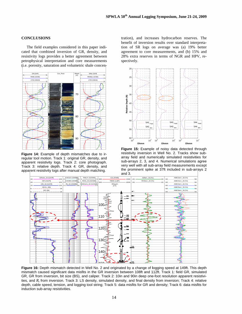
• Detection of adverse borehole environmental con-ditions or tool malfunctioning. Figures 14, 15 and 16 show examples of log-

quality problems detected through inversion and di-agnosed by abnormal and local-depth variations of data misfit. Depth matching of logs is necessary because in-version assumes a common set of bed boundaries for all the input logs. Figure 14 shows an example of depth mismatch due to the irregular motion of the tool string in Well No. 1. Figure 15 shows an example of noisy raw resistiv-ity data in Well No. 2. The abnormal spike in sub-array numbers 2 and 3 at 37ft could not be repro-duced and correlated with other sub-array measure-ments. Therefore, it can be attributed to tool malfunc-tioning of sub-arrays 2 and 3 at that depth. Figure 16 shows one more example of depth mismatch due to a change of logging speed in Well No. 2. Although log depth matching was not imple-mented in this well, data misfits associated with GR inversion were relatively high in the depth interval 108ft-112ft. The reason for this behavior was a change of logging speed at 149ft. Speed measure-ments are commonly referred to the zero-point of the tool, which in that case is at the bottom of the tool string. Thus, when the bottom of the tool was located at 149ft the GR sensor was located exactly at 112ft. Although density and resistivity logs were also af-fected by the change of logging speed, the corre-sponding effect was negligible because at that instant the sensors were located within a shaly interval of negligible petrophysical importance.


14

CONCLUSIONS The field examples considered in this paper indi-cated that combined inversion of GR, density, and resistivity logs provides a better agreement between petrophysical interpretation and core measurements (i.e. porosity, saturation and volumetric shale concen-

tration), and increases hydrocarbon reserves. The benefit of inversion results over standard interpreta-tion of SR logs on average was (a) 19% better agreement to core measurements, and (b) 15% and 28% extra reserves in terms of NGR and HPV, re-spectively.

GR (GAPI)

20. 90.RHOB (G/CM3)

2. 2.5AT90 (OHM.M)

1. 20.

Core_Photo RDepth(FT)

GRds (GAPI)20. 90.

RHOBds (G/CM3)2. 2.5

AT90 (OHM.M)1. 20.

70

80

90

Figure 14: Example of depth mismatches due to ir-regular tool motion. Track 1: original GR, density, and apparent resistivity logs. Track 2: core photograph. Track 3: relative depth. Track 4: GR, density, and apparent resistivity logs after manual depth matching.

100 101

20

25

30

35

40

45

50

55

60

Ohmm

Rel

ativ

e D

epth

(ft)

SA2 Field

SA2 Sim

100 101

Ohmm

SA3 Field

SA3 Sim

100 101

Ohmm

SA4 Field

SA4 Sim

Figure 15: Example of noisy data detected through resistivity inversion in Well No. 2. Tracks show sub-array field and numerically simulated resistivities for sub-arrays 2, 3, and 4. Numerical simulations agree very well with all sub-array field measurements except the prominent spike at 37ft included in sub-arrays 2 and 3.

100

110

120

130

140

150

GRsim_SI (GAPI)20. 100.

GR (GAPI)20. 100.

GR_SI (GAPI)20. 100.

HCAL (IN)8. 18.

BS (IN)8. 18.

AHO10 (OHMM)0.1 100.

AHO90 (OHMM)0.1 100.

Rt_SI (OHMM)0.1 100.

RHLA (G/CM3)2. 2.5

RHO_SI (G/CM3)2. 2.5RHOsim_SI (G/CM3)2. 2.5

CS (F/HR)300. 1300.

TENS (LBF)500. 1500.

RDepth(FT)

GRerr_SI (%)-20. 20.

RHOerr_SI (%)-20. 20.

AIBC2err_SI (%)-50. 50.

AIBC4err_SI (%)-50. 50.

AIBC3err_SI (%)-50. 50.

AIBC5err_SI (%)-50. 50.

AIBC6err_SI (%)-50. 50.

Figure 16: Depth mismatch detected in Well No. 2 and originated by a change of logging speed at 149ft. This depth mismatch caused significant data misfits in the GR inversion between 108ft and 112ft. Track 1: field GR, simulated GR, GR from inversion, bit size (BS), and caliper. Track 2: 10in and 90in deep one-foot resolution apparent resistivi-ties, and Rt from inversion. Track 3: LS density, simulated density, and final density from inversion; Track 4: relative depth, cable speed, tension, and logging tool string; Track 5: data misfits for GR and density; Track 6: data misfits for induction sub-array resistivities.


15

Field examples of inversion indicated that the minimum bed thickness necessary for successful de-terministic inversion was approximately 0.7 ft. How-ever, the minimum bed size could be less than 0.7 ft in cases of wells logged with high sampling rates and logging operations with good depth control (e.g. shal-low wells, onshore wells, etc). The most critical step for inversion was the detec-tion of bed boundaries. Slight perturbations applied to bed boundaries caused significant changes of in-verted results, especially across very thin beds. Field cases confirmed that inflection points of LS or com-pensated density measurements are the best choice for detecting bed boundaries because the density log exhibits the highest vertical resolution among triple-combo logs (GR, density, neutron, and resistivity), has the maximum effect on porosity calculations, and is associated with a spatially symmetric FSF. Bore-hole measurements such as micro-resistivity could be used to detect boundaries when the tool is mounted on the same density pad. The least desirable option for bed-boundary detection are GR and resistivity logs. Additionally, even though HR logs can detect thinner beds than SR logs, the latter are preferred over the former because they can lead to very thin layers where inversion is not reliable (due to high non-uniqueness) or cause false layer detection due to abnormal log fluctuations due to measurement noise and sudden variations of borehole environmental conditions. Although the combined inversion method does not require high-resolution borehole images, core measurements, or repeat sections, this information is important to cross-validate both detected bed bounda-ries and petrophysical interpretations obtained from inversion results. The inclusion of GR logs in the combined inver-sion of density and resistivity is necessary because of the low vertical resolution of GR logs compared to that of density and resistivity logs. The examples of inversion undertaken in this paper indicate that at least half of the improvement in core matching and hydrocarbon reserves with respect to standard well-log interpretation is due to the enhancement of GR logs through inversion. FSFs required for density and GR inversion should be faithful representations of actual measure-ment acquisition. The FSFs for “UT Longhorn Tools” were calculated for generic logging tools. As a result, they had to be adjusted to match the corre-sponding FSFs of commercial tools. We performed this adjustment by “stretching” the UT Longhorn FSFs by a certain factor until securing a good match between numerical simulated and measured well logs. In so doing, we assumed an arrangement of sensors and sources similar to those of “UT Long-

horn Tools” FSFs. The calculated stretching factors were as follows: 2.1 for SGT/HGNS GR, 1.10 and 3.7 for LS and SS PEX density measurements, re-spectively, and 1.3 and 3.9 for the LS and SS LDT density measurements, respectively. Selection of sensors for inversion depends on borehole environmental conditions and log quality. For example, in one of the field cases considered, resistivity inversion results improved by neglecting deep sub-arrays that were highly affected by layer dip. In addition, noisy sub-arrays, borehole-affected mono-sensor density data, or shallow sub-arrays af-fected by severe washouts should not be included as input to the combined inversion. Large data misfits could indicate the need for ad-ditional layers, or marginal quality of logs due to borehole environmental conditions or tool malfunc-tioning. They could also indicate violation of model assumptions implicit in the numerical simulation of well logs, such as non-horizontal layers, non-piston-like radial invasion, electrical anisotropy, etc. In gen-eral, our experience with combined inversion of well logs shows that the method is exceedingly valuable to diagnose measurement biases often unheeded by standard well-log interpretation. NOMENCLATURE a Archie’s tortuosity factor ( )C x cost function used for inversion

Csh volumetric shale concentration, (frac.) Csh-cf Csh cutoff applied for reserves, (frac.)

)(xd vector of numerically simulated logs 0d vector of field measurements ( )e x vector of data misfits

FSF matrix constructed with 1D FSFs GR total gamma-ray measurement, (GAPI)

rawiGR raw GR at a given depth i, (GAPI)

GRi filtered or SR GR at a given depth i, (GAPI) GRs gamma-ray reading in clean sands, (GAPI) GRsh gamma-ray reading in shales, (GAPI) HPV hydrocarbon pore volume, (hydrocarbon-ft) i depth index m Archie’s cementation exponent n Archie’s saturation exponent NGR Net-to-gross ratio, (frac.) payi pay flag RE relative error, (%) Rt true formation resistivity, (Ohm-m) Rw connate water resistivity, (Ohm-m) Rwb bound-water resistivity, (Ohm-m) Rxo invaded zone resistivity, (Ohm-m) R2 linear correlation coefficient, (frac.)


16

Swb bound-water saturation, (frac.) Sws non-shale water saturation, (frac.) Sws-cf Sws cutoff applied for reserves, (frac.) Swt total water saturation, (frac.) x vector containing unknown layer properties

0x prior model used for inversion regularization Δhi vertical depth increment, (ft) φs non-shale porosity, (frac.) φs-cf φs cutoff applied for reserves, (frac.) φsh total porosity of wet shale, (frac.) φt total porosity, (frac.) λ stabilization parameter for inversion ρh density of hydrocarbon, (gr/cc) ρm density of matrix, (gr/cc) ρr bulk rock density, (gr/cc) ρsh density of wet shale, (gr/cc) ρw density of water, (gr/cc) ACKNOWLEDGEMENTS We thank BHP Billiton for the opportunity to work on this project during a 2007 summer internship by Jorge Sanchez-Ramirez. The authors wish to thank BHP Billiton, BP, Chevron U.S.A. Inc., Sta-toilHydro USA E&P Inc., and Nexen Petroleum Off-shore U.S.A. Inc. for permission to publish this pa-per. A note of special gratitude goes to Andy Brickell from BHP Billiton for his continuous technical sup-port. The work was partially funded by The Univer-sity of Texas at Austin’s Research Consortium on Formation Evaluation. REFERENCES Barber, T. D. and R. A. Rosthal, 1991, Using a multi-

array induction tool to achieve high-resolution logs with minimum environmental effects: 66th Annual Technical Conference and Exhibition, SPE, Expanded Abstracts, Paper SPE22725, Dal-las, TX, October 6-9.

Best, D. L., Gardner, J. S., and Dumanoir, J. L., 1980, A computer-processed wellsite log computation, Paper Z presented at the 1978 Annual SPWLA Symposium - and paper SPE 9039 presented at the 1980 SPE Rocky Mountain Meeting Proceed-ings, Casper, WY, May 14-16.

Campbell, C. V., 1967, Lamina, lamina set, bed and bedset: Sedimentology, v8, p. 7-26.

Clavier, C., Coates, G., and Domanoir, J., 1977, The theoretical and experimental bases for the dual water model for the interpretation of shaly sands, SPE 6859, Proceedings of the AIME Annual Technical Conference and Exhibition: Society of Petroleum Engineers.

Dewan, J. T., 1983, Essentials of modern open-hole log interpretation: PennWell Publishing Com-pany.

Hansen, P. C., 1998, Rank-deficient and discrete ill-posed problems: numerical aspects of linear in-version, Society of Industrial and Applied Mathematics, The United States of America.

Liu, Z., Torres-Verdín, C., Wang, G. L., Mendoza, A., Zhu, P., and Terry, R., Joint inversion of den-sity and resistivity logs for the improved petro-physical assessment of thinly-bedded clastic rock formations, 48th Annual Logging Symposium Transactions: Society of Petrophysicists and Well Log Analysts, Austin, TX, June 3-6.

Mendoza, A., Torres-Verdín, C., and Preeg, W. E., 2007, Rapid simulation of borehole nuclear meas-urements using approximate spatial flux-scattering functions, 48th Annual Logging Sym-posium Transactions: Society of Petrophysicists and Well Log Analysts, Austin, TX, June 3-6.

Passey, Q. R., Dahlberg, K. E., Sullivan, K. B., Yin, H., Brackett, R. A., Xiao, Y. H., and Guzmán-Garcia, A.G., 2006, Petrophysical evaluation of hydrocarbon pore-thickness in thinly bedded clas-tic reservoirs: AAPG Archie Series, n. 1. Tulsa.

Sanchez-Ramirez, J. A., 2009, Field examples of the combined petrophysical inversion of gamma-ray, density, and resistivity logs acquired in thinly-bedded clastic rock formations, M.Sc. Thesis, The University of Texas at Austin, Texas.

Thomas, E. C., and Stieber, S. J., 1975, The distribu-tion of shale in sand stones and its effects upon porosity, paper T in 16th Annual Logging Sympo-sium Transactions: Society of Professional Well Log Analysts.

Tikhonov, A. N., Arsenin, V. Y., 1977, Solutions of ill-posed problems: Wiley. New York. Wang, G. L., Torres-Verdín, C., Salazar, J. M., and

Voss, B., 2009, Fast 2D inversion of large bore-hole EM induction data sets with an efficient Fré-chet-derivative approximation: Geophysics, v. 74, no. 1, pp. E75-E91.

Zhang, G. J., Wang, H. M., and Wang, G. L., 1995, A.C. logging response in stratified media, Chinese Journal of Geophysics, v. 38, n. 6, pp. 841-849.

Zhang, G. J., Wang, G. L., and Wang, H. M, 1999, Application of novel basis functions in a hybrid method simulation of the response of induction logging in axisymmetrical stratified media, Radio Science, v. 34, no. 1, pp. 19-26.

field examples of the combined petrophysical inversion of ... · field examples of the combined...

Documents