Field Laboratory for Ocean Sea State Investigation and Experimentation:

FLOSSIE

Intra-Measurement Evaluation of 6N Wave Buoy Systems

R.E. Jensen1, V.R. Swail2, R. H. Bouchard3, R.E. Riley3, T.J. Hesser1, M. Blaseckie4 and C. MacIsaac4

1US Army Engineer Research and Development Center

Coastal and Hydraulics Laboratory (ERDC-CHL)

2Environment Canada

3National Oceanic and Atmospheric Administration

National Data Buoy Center (NOAA-NDBC)

4AXYS Technologies

ABSTRACT

Point-source wave measurements have and continue to be an important element in assessing the wave

conditions, aiding the Weather Prediction Center’s evaluations of their forecast, used in data assimilation,

wave modeling investigations, used in algorithms estimating waves from satellite-based altimeters,

climate studies, wave energy resource assessments and other applications. The work presented here

assesses the similarities/differences between various sensor/payload packages housed in a 6N NOMAD

buoy that is deployed in Monterey Canyon as part of the Buoy Farm, and a comprehensive intra-

measurement evaluation.

INTRODUCTION

The National Oceanic and Atmospheric Administration’s (NOAA) National Data Buoy Center (NDBC)

and Environment Canada (EC) have been operating networks of meteorological and wave measurement

sites in the Atlantic, Pacific, Gulf of Mexico and Great Lakes for the past four decades (Timpe and Van

de Voorde, 1995; Skey et al. 1995). The platforms used by these two agencies vary from discus buoys of

varying sizes to a standard 6-m (6N) Navy Oceanographic and Meteorological Automatic Device, or

NOMAD buoy. These data sets have been instrumental in the evaluation of wave model results in a

hindcast or forecasting mode, used by the satellite-based remote sensing community building algorithms

estimating the significant wave height from altimeters, and SAR images, and in research efforts studying

the role of surface-gravity wind waves in air-sea interactions and surface flux estimations.

Over the period of record there have been modifications to the platform, sensor and payload (on-board

analysis package) that can affect the long-term records (Gemmerich et al., 2011) that have been used to

assess the trends in the wave climate (e.g. Allan and Komar, 2008; Ruggerio et al., 2010; and Menéndez

et al., 2008). Using altimeter data as a common reference, Durrant et al. (2009) compared EC and

NOAA-NDBC wave height data and found a systematic difference of 10-percent in significant wave

height reported by EC and NDBC. Large portions of the point-source measurements were derived from

6N buoy systems. With these results, and NDBC planning to decommission all of their NOMAD buoys,

it became a necessity to construct a meaningful experiment in hopes of answering some of the questions

regarding these long-standing data records.

In 2012, a plan for an experiment Field Laboratory for Ocean Sea State Investigation and

Experimentation (FLOSSIE1) was developed, where a 6N hull would be configured with all historical

sensor, and payload packages used by NDBC during the past four decades. Gemmrich et al. (2011)

identified the various configuration changes in seven wave platforms located in the Pacific. They

identified over time where the hull, payload, and processor changes occurred at these sites. The changes

reflected discontinuities in the data records from -0.66-m to +0.59-m. If these different configurations

were placed in one hull and evaluated it would provide a means to account for temporal changes in

payloads and sensor systems by NDBC while evaluating the accuracy of the archive data sets. In addition

to the NDBC sensor (and payload systems), AXYY® has provided their new sensor system (TRIAXYS)

and two payloads that will be used to directly assess differences between EC and NDBC 6N buoy records.

FLOSSIE is part of the continued effort of the U.S. Army Corps of Engineer (USACE) Engineer

Research and Development Center’s Coastal and Hydraulics Laboratory (CHL) to test and evaluate wave

measurements. This has been identified in the US IOOS Waves Plan (IOOS, 2009). Insights of the Test

and Evaluation have been documented in Swail et al. (2009) and Jensen et al. (2011). In a subsequent

paper (Luther et al. 2013) provided detailed procedures to be followed, also identified in the Alliance for

Coastal Technologies (ACT/UMCES, 2012). The recurring theme across these documents was the need

to test and evaluate historical and existing wave measurement platforms and seek a standard evaluation

for new technological advancements.

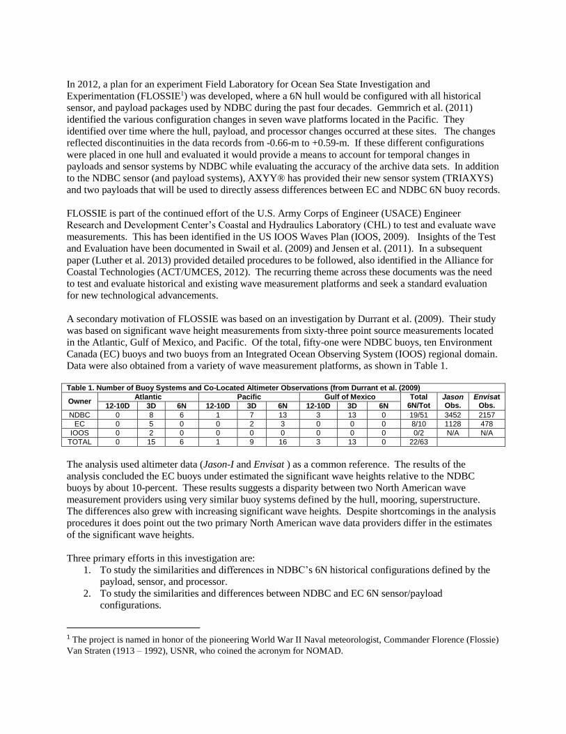
A secondary motivation of FLOSSIE was based on an investigation by Durrant et al. (2009). Their study

was based on significant wave height measurements from sixty-three point source measurements located

in the Atlantic, Gulf of Mexico, and Pacific. Of the total, fifty-one were NDBC buoys, ten Environment

Canada (EC) buoys and two buoys from an Integrated Ocean Observing System (IOOS) regional domain.

Data were also obtained from a variety of wave measurement platforms, as shown in Table 1.

Table 1. Number of Buoy Systems and Co-Located Altimeter Observations (from Durrant et al. (2009)

Owner Atlantic Pacific Gulf of Mexico Total

6N/Tot Jason Obs.

Envisat Obs. 12-10D 3D 6N 12-10D 3D 6N 12-10D 3D 6N

NDBC 0 8 6 1 7 13 3 13 0 19/51 3452 2157

EC 0 5 0 0 2 3 0 0 0 8/10 1128 478

IOOS 0 2 0 0 0 0 0 0 0 0/2 N/A N/A

TOTAL 0 15 6 1 9 16 3 13 0 22/63

The analysis used altimeter data (Jason-I and Envisat ) as a common reference. The results of the

analysis concluded the EC buoys under estimated the significant wave heights relative to the NDBC

buoys by about 10-percent. These results suggests a disparity between two North American wave

measurement providers using very similar buoy systems defined by the hull, mooring, superstructure.

The differences also grew with increasing significant wave heights. Despite shortcomings in the analysis

procedures it does point out the two primary North American wave data providers differ in the estimates

of the significant wave heights.

Three primary efforts in this investigation are:

1. To study the similarities and differences in NDBC’s 6N historical configurations defined by the

payload, sensor, and processor.

2. To study the similarities and differences between NDBC and EC 6N sensor/payload

configurations.

1 The project is named in honor of the pioneering World War II Naval meteorologist, Commander Florence (Flossie)

Van Straten (1913 – 1992), USNR, who coined the acronym for NOMAD.

3. To investiagte the accuracy in estimating directional properties derived from non-symmetric hull

configurations?

FLOSSIE AND THE BUOY FARM

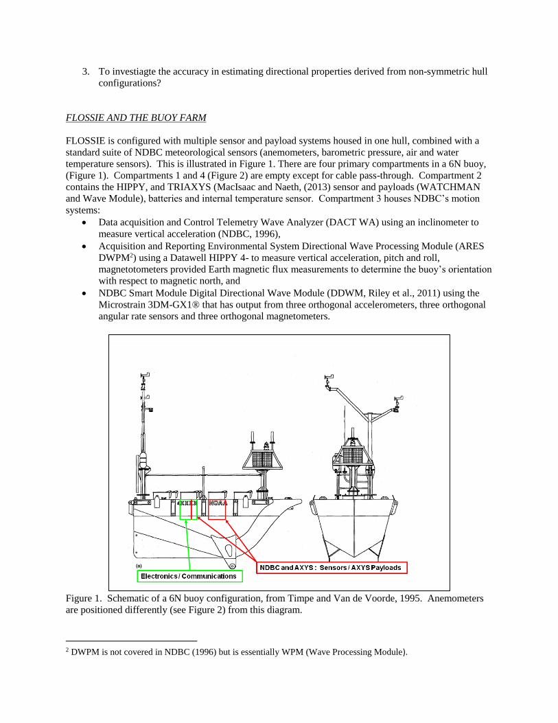
FLOSSIE is configured with multiple sensor and payload systems housed in one hull, combined with a

standard suite of NDBC meteorological sensors (anemometers, barometric pressure, air and water

temperature sensors). This is illustrated in Figure 1. There are four primary compartments in a 6N buoy,

(Figure 1). Compartments 1 and 4 (Figure 2) are empty except for cable pass-through. Compartment 2

contains the HIPPY, and TRIAXYS (MacIsaac and Naeth, (2013) sensor and payloads (WATCHMAN

and Wave Module), batteries and internal temperature sensor. Compartment 3 houses NDBC’s motion

systems:

Data acquisition and Control Telemetry Wave Analyzer (DACT WA) using an inclinometer to

measure vertical acceleration (NDBC, 1996),

Acquisition and Reporting Environmental System Directional Wave Processing Module (ARES

DWPM2) using a Datawell HIPPY 4- to measure vertical acceleration, pitch and roll,

magnetotometers provided Earth magnetic flux measurements to determine the buoy’s orientation

with respect to magnetic north, and

NDBC Smart Module Digital Directional Wave Module (DDWM, Riley et al., 2011) using the

Microstrain 3DM-GX1® that has output from three orthogonal accelerometers, three orthogonal

angular rate sensors and three orthogonal magnetometers.

Figure 1. Schematic of a 6N buoy configuration, from Timpe and Van de Voorde, 1995. Anemometers

are positioned differently (see Figure 2) from this diagram.

2 DWPM is not covered in NDBC (1996) but is essentially WPM (Wave Processing Module).

All real-time NDBC and AXYS® data are transmitted separately via IRIDIUM communications. The

3DMG and AXYS® original time series are also stored to disks onboard. These disks will be recovered

during scheduled maintenance runs to the buoy on a yearly basis. There are a total of five different data

sets recovered from FLOSSIE:

1. NDBC: Inclinometer / DACT WA(non-directional).

2. NDBC: HIPPY/Magnetometer DWPM (original sensor/payload package to estimate directional

waves)

3. NDBC: Motion Sensor MicroStrain 3DM-GX1® DDWM

4. AXYS®: TRIAXYS Next Wave II Directional Wave Sensor / Wave Module (new payload

package used for directional wave measurements, e.g. TRIAXYS buoys).

5. AXYS®: EC-Watchman (strapped down accelerometer used by Environment Canada)

FLOSSIE is the focal point of this paper, however there is much more to the intra-measurement

evaluation that is part of the Buoy Farm located in Monterey Bay Canyon (Figure 3). Besides FLOSSIE

containing multiple sensor/payloads, three other wave measurement systems have been deployed. This is

one of two primary wave measurement evaluation locations defined by ACT/UMCES (2012), and Luther

et al. (2013). The Buoy Farm now consists of FLOSSIE, an NDBC 3-m aluminum discus hull NDBC

discus buoy containing two sensor/payload packages (HIPPY/ MicroStrain 3DM-GX1® , Riley et al.,

2011), and a Datawell® Directional Waverider buoy operated by the Coastal Data Information Program

(CDIP, http://cdip.ucsd.edu/).

6. NDBC: HIPPY / DWPM payload (directional estimates)

7. NDBC: MicroStrain3DM-GX1® / DDWM payload (directional estimates)

8. CDIP/USACE: Datawell® Directional Wavrider (directional estimates)

Figure 2. Picture of FLOSSIE dockside at NDBC, (provided by R. Riley, NDBC).

The Datawell® Directional Waverider buoy was selected as the relative reference to be used in all wave

intra-measurements evaluations (IOOS, 2009; ACT/UMCES, 2012 and Luther et al. 2013). This is not to

suggest a Datawell buoy is the standard for wave measurements; it was selected because these systems

have been used operationally for over forty-years by a wide variety of users, including CDIP and the

international offshore oil and gas industry. Data are transmitted from these systems on a sixty or thirty

minute interval via IRIDIUM communication protocols. All raw data (e.g. time series) is saved to flash

drives and internally stored onboard. These data sets will be retrieved during scheduled maintenance of

the various buoys in Monterey Canyon. The Datawell transmits the raw time series directly to the CDIP

operational center on a sixty minute interval via Iridium.

AXYS® has also offered an additional TRIAXYS sensor/payload package to be mounted on an NDBC

3D buoy and a complete TRIAXYS buoy system. Plans are underway to add these systems to the

existing array of wave measurement systems presently deployed in the Buoy Farm.

MEASURED DATA FROM THE BUOY FARM

In general there are two primary data files for each of the eight wave measurement systems. The first data

set contains the integral wave parameters: significant wave height (Hmo), wave period (the peak spectral

wave period Tp, and/or a mean wave period Tmean), and an estimate of the wave direction (mean wave

direction at the peak frequency θmean(fm). AXYS® systems provide additional integral wave parameters

derived from the raw time series: Have (average wave height), Hmax (maximum wave height), Tmax

(maximum wave period), H1/10, T1/10 (highest one-tenth wave height, and wave period), Tave (average wave

period), Hsig, Tsig (significant wave height and period defined from the average of the highest one third

wave height in the record), Tp5 (peak period READ method) , and the wave steepness. Meteorological

instrumentation onboard NDBC 46042 and 46FLO provides measurements of:

Wind Speed, U5 / Wind Gust, UG

Wind Direction, θwind,

Barometric Pressure, Bp

Air and Water3 temperature, Tair, Twater.

The second data set consists of spectral and directional estimates derived from the time series of the buoy

motion. These parameters are defined by:

𝑆(𝑓, 𝜃) = 𝑆(𝑓)[𝑎1 ∙ cos 𝜃 + 𝑏1 ∙ cos 𝜃 + 𝑎2 ∙ cos 2𝜃 + 𝑏2 ∙ sin 2𝜃 + 𝑎2 ∙ cos 2𝜃 + 𝑏2 ∙ sin 2𝜃+ 𝑏3 ∙ sin 3𝜃 + 𝑏4 ∙ sin 4𝜃 + ⋯]

(1)

S(f,θ) is the two dimensional wave spectra defined by the range in frequencies (f), and direction (θ). S(f)

is the frequency spectra and sometimes defined by a0 where 𝑎0 = 𝑆(𝑓)

𝜋⁄ . The terms defined by a1, b1, a2,

b2, … are the Fourier coefficients. Directional buoy measurements return the First-5 components in the

infinite Fourier series (a0, a1, b1, a2, b2) defined in Equation 1. The Datawell and AXYS systems spectral

estimates are defined by the First-5 Fourier coefficients defined at each frequency band.

The NDBC computes Fourier coefficients onboard the buoy but recasts them as:

3 The Datawell Directional Waverider is equipped with a water temperature sensor.

𝑆(𝑓, 𝜃) = 𝐶11 ∙ {

[12⁄ + 𝑟1 ∙ cos(𝜃 − 𝜃1) + 𝑟2 cos(2(𝜃 − 𝜃2))]

𝜋} (2)

C11 is equivalent to S(f) in Equation 1. The directional Fourier coefficients r1 and r2 are related to the a1,

b1, a2, b2 values as:

𝑟1 =

√𝑎12 + 𝑏1

2

𝑎0⁄ (3)

𝑟2 =

√𝑎22 + 𝑏2

2

𝑎0⁄ (4)

𝜃1 = tan−1 (𝑏1

𝑎1⁄ ) (5)

𝜃2 = (12⁄ ) tan−1 (

𝑏2𝑎2

⁄ ) (6)

NDBC represents the mean directional components (θ1 and θ2) by α1 and α2 where:

𝛼𝑛 = (3𝜋2⁄ ) − 𝜃𝑛 (7)

where αn represents the direction FROM which the waves originate following the conventions of the

World Meteorological Office (WMO, 1995) and Frigaard et al. (1997). There is an ambiguity in θ2. This

value is either θ2 or (θ2+π) whichever minimizes the difference between θ1 and θ2.

Altimeter estimates (track positions of various altimeters, from GLOBwave, http://globwave.ifremer.fr/ )

of the significant wave height will be accessed and compared to the data provided from FLOSSIE’s

multiple sensor/payload packages. An example for a one month period is displayed in Figure 3. The blue

dots represent the significant wave height estimates from four altimeters (JASON-1, JASON-2,

CRYOSAT, and SARL). There may be sufficient co-located altimeter and buoy data to perform a

similar analysis performed by Durrant et al. (2009), to support or dispute the 10-percent differences they

noted.

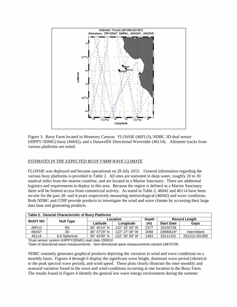
Figure 3. Buoy Farm located in Monterey Canyon. FLOSSIE (46FLO), NDBC 3D dual sensor

(HIPPY/3DMG) buoy (46042), and a Datawell® Directional Waverider (46114). Altimeter tracks from

various platforms are noted.

ESTIMATES IN THE EXPECTED BUOY FARM WAVE CLIMATE

FLOSSIE was deployed and became operational on 28 July 2015. General information regarding the

various buoy platforms is provided in Table 2. All sites are stationed in deep water, roughly 20 to 30

nautical miles from the nearest coastline, and are located in a Marine Sanctuary. There are additional

logistics and requirements to deploy in this area. Because the region is defined as a Marine Sanctuary

there will be limited access from commercial activity. As noted in Table 2, 46042 and 46114 have been

on-site for the past 28- and 4-years respectively measuring meteorological (46042) and wave conditions.

Both NDBC and CDIP provide products to investigate the wind and wave climate by accessing their large

data base and generating products.

Table 2. General Characteristic of Buoy Platforms

BUOY NO Hull Type Location Depth

(m)

Record Length

Latitude Longitude Start Date Gaps

46FLO 6N 36° 40'14" N 122° 33' 43" W 2377 20150728 -

460421 3D 36° 47'29" N 122° 27' 06" W 2098 199806192 Intermittent

46114 0.9 Spherical 36° 43'00" N 122° 30' 59" W 1463 20111101 201212-201305 1Dual sensor system (HIPPY/3DMG) start date 200910 2Start of directional wave measurements. Non-directional wave measurements started 19870709.

NDBC routinely generates graphical products depicting the variation in wind and wave conditions on a

monthly basis. Figures 4 through 6 display the significant wave height, dominant wave period (identical

to the peak spectral wave period), and wind speed. These plots clearly illustrate the inter-monthly and

seasonal variation found in the wave and wind conditions occurring at one location in the Buoy Farm.

The results found in Figure 4 identify the general low wave energy environment during the summer

months. Moving into the fall and winter seasons, the mean significant wave height increases by 1-m, and

for this population, the maximum observed significant wave height approaches 10-m, nearly a factor of

2.5 greater than what occurred in July, where the lowest energy exist. There is a reasonable expectation

to observe storm peak events above 6-m during the FLOSSIE deployment. Similarly, there are periods

where significant wave heights can be less than 0.5-m. The other observation from Figure 4 is the range

in the standard deviation is relatively consistent month to month with exception to the summer season.

This suggests the probability distribution defining the range in significant wave heights occupies a very

limited defined interval.

The west coast of the US (California, Oregon and Washington) wave climate is dominated by long-period

swell energy derived from meteorological events developing in the western Pacific Ocean and migrating

in an easterly direction. These conditions resonate in Figure 5, where the mean dominant wave period

range from 10- to about 12-s, and have a have a similar trend as in the significant wave height monthly

variation. The standard deviation from month to month is + 2.5-s suggesting there is a very small range

in wave periods found in the probability distribution. For the larger and more distant events, the

dominant wave periods exceed 20-s each and every month. In many cases (as will be shown in the latter

section) there are multiple wave systems occurring at one time, where local wind-seas are created by the

winds in the region and generally running along a much different wave direction compared to the swells.

Local winds will play a role in the FLOSSIE study. The variation in the mean wind speed (Figure 6) on

an inter-monthly interval is on the order of 3kt (~1.5m/s). The variation about the mean wind speed

consistently runs at about + 3kt (~1.5m/s) suggesting again the probability distribution is narrow

occupying a very small range in wind speeds. There are times during the winter season where the local

winds can exceed 30kts (~15m/s) for a peak storm event. The mean and maximum wind speed trend is

similar to the wave parameters; however the minimum monthly condition occurs in September rather than

in August. The maximum mean wind speeds also occur from March through June rather than in the

winter months found in Figures 4 and 5. This could suggest that the number of meteorological storm

events increases in the spring, however the amount of energy created from the local winds will have a

limited impact on the wave climate.

It does appear from data obtained at 46042, that the wave climate is at times well behaved. The inter-

monthly mean variation is rather constant at about 1.5-m in wave height, 2-s in wave period and for the

wind speed about 3kt (1.5m/s). There is a distinct seasonal variation for the waves that could be

complicated by the shift in conditions found in the winds especially in the spring. This simple analysis

that is mainly observational and qualitative will provide a certain degree of understanding when the data

from FLOSSIE begins to flow and the analysis is performed.

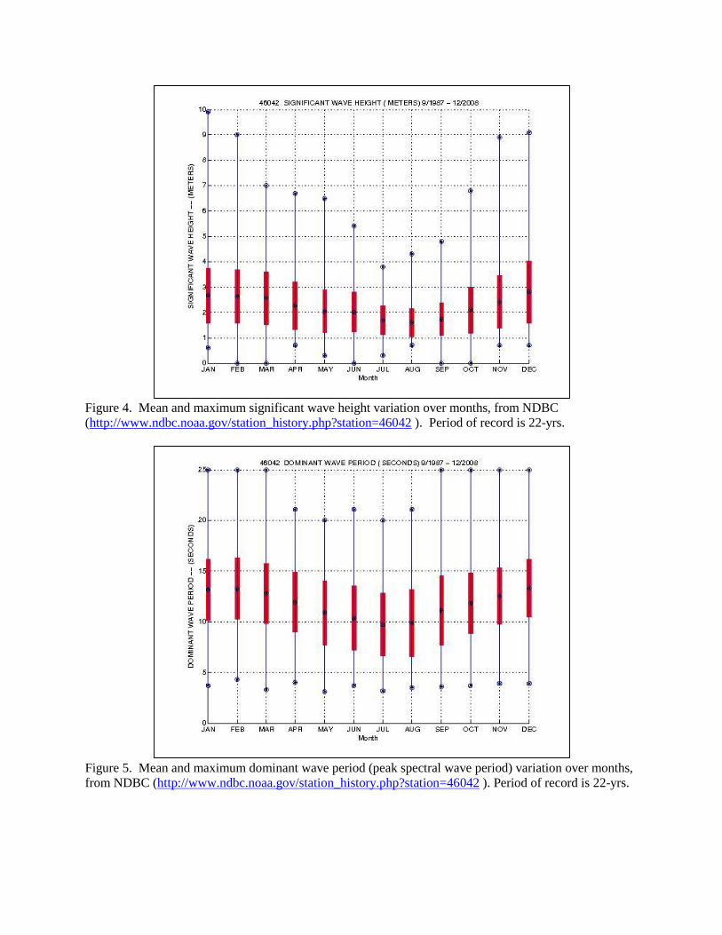
Figure 4. Mean and maximum significant wave height variation over months, from NDBC

(http://www.ndbc.noaa.gov/station_history.php?station=46042 ). Period of record is 22-yrs.

Figure 5. Mean and maximum dominant wave period (peak spectral wave period) variation over months,

from NDBC (http://www.ndbc.noaa.gov/station_history.php?station=46042 ). Period of record is 22-yrs.

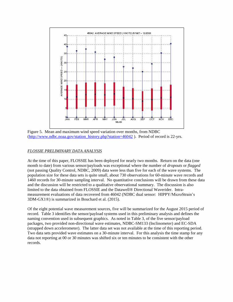
Figure 5. Mean and maximum wind speed variation over months, from NDBC

(http://www.ndbc.noaa.gov/station_history.php?station=46042 ). Period of record is 22-yrs.

FLOSSIE PRELIMINARY DATA ANALYSIS

At the time of this paper, FLOSSIE has been deployed for nearly two months. Return on the data (one

month to date) from various sensor/payloads was exceptional where the number of dropouts or flagged

(not passing Quality Control, NDBC, 2009) data were less than five for each of the wave systems. The

population size for these data sets is quite small, about 730 observations for 60-minute wave records and

1460 records for 30-minute sampling interval. No quantitative conclusions will be drawn from these data

and the discussion will be restricted to a qualitative observational summary. The discussion is also

limited to the data obtained from FLOSSIE and the Datawell® Directional Waverider. Intra-

measurement evaluations of data recovered from 46042 (NDBC dual sensor: HIPPY/MicroStrain’s

3DM-GX1®) is summarized in Bouchard et al. (2015).

Of the eight potential wave measurement sources, five will be summarized for the August 2015 period of

record. Table 3 identifies the sensor/payload systems used in this preliminary analysis and defines the

naming convention used in subsequent graphics. As noted in Table 3, of the five sensor/payload

packages, two provided non-directional wave estimates, NDBC-SM133 (Inclinometer) and EC-SDA

(strapped down accelerometer). The latter data set was not available at the time of this reporting period.

Two data sets provided wave estimates on a 30-minute interval. For this analysis the time stamp for any

data not reporting at 00 or 30 minutes was shifted six or ten minutes to be consistent with the other

records.

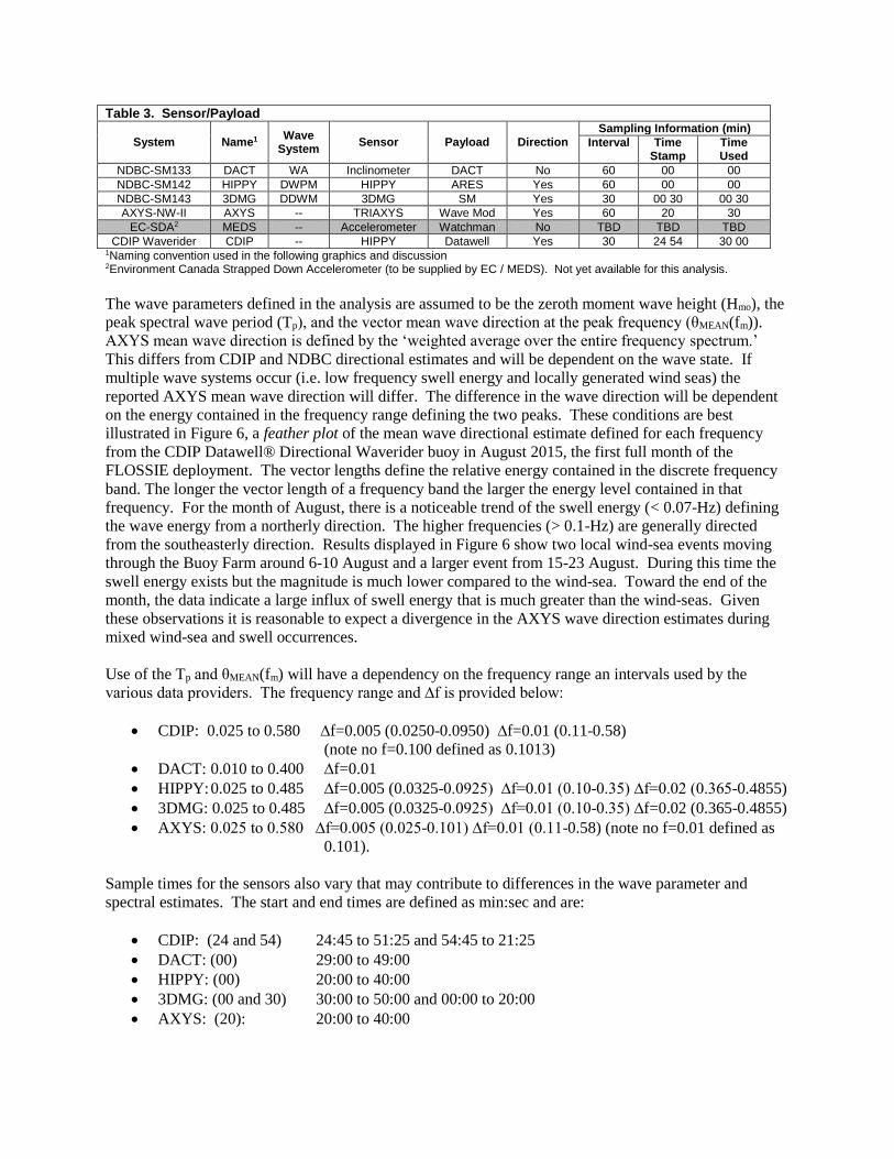
Table 3. Sensor/Payload

System Name1 Wave

System Sensor Payload Direction

Sampling Information (min)

Interval Time Stamp

Time Used

NDBC-SM133 DACT WA Inclinometer DACT No 60 00 00

NDBC-SM142 HIPPY DWPM HIPPY ARES Yes 60 00 00

NDBC-SM143 3DMG DDWM 3DMG SM Yes 30 00 30 00 30

AXYS-NW-II AXYS -- TRIAXYS Wave Mod Yes 60 20 30

EC-SDA2 MEDS -- Accelerometer Watchman No TBD TBD TBD

CDIP Waverider CDIP -- HIPPY Datawell Yes 30 24 54 30 00 1Naming convention used in the following graphics and discussion 2Environment Canada Strapped Down Accelerometer (to be supplied by EC / MEDS). Not yet available for this analysis.

The wave parameters defined in the analysis are assumed to be the zeroth moment wave height (Hmo), the

peak spectral wave period (Tp), and the vector mean wave direction at the peak frequency (θMEAN(fm)).

AXYS mean wave direction is defined by the ‘weighted average over the entire frequency spectrum.’

This differs from CDIP and NDBC directional estimates and will be dependent on the wave state. If

multiple wave systems occur (i.e. low frequency swell energy and locally generated wind seas) the

reported AXYS mean wave direction will differ. The difference in the wave direction will be dependent

on the energy contained in the frequency range defining the two peaks. These conditions are best

illustrated in Figure 6, a feather plot of the mean wave directional estimate defined for each frequency

from the CDIP Datawell® Directional Waverider buoy in August 2015, the first full month of the

FLOSSIE deployment. The vector lengths define the relative energy contained in the discrete frequency

band. The longer the vector length of a frequency band the larger the energy level contained in that

frequency. For the month of August, there is a noticeable trend of the swell energy (< 0.07-Hz) defining

the wave energy from a northerly direction. The higher frequencies (> 0.1-Hz) are generally directed

from the southeasterly direction. Results displayed in Figure 6 show two local wind-sea events moving

through the Buoy Farm around 6-10 August and a larger event from 15-23 August. During this time the

swell energy exists but the magnitude is much lower compared to the wind-sea. Toward the end of the

month, the data indicate a large influx of swell energy that is much greater than the wind-seas. Given

these observations it is reasonable to expect a divergence in the AXYS wave direction estimates during

mixed wind-sea and swell occurrences.

Use of the Tp and θMEAN(fm) will have a dependency on the frequency range an intervals used by the

various data providers. The frequency range and ∆f is provided below:

CDIP: 0.025 to 0.580 ∆f=0.005 (0.0250-0.0950) ∆f=0.01 (0.11-0.58)

(note no f=0.100 defined as 0.1013)

DACT: 0.010 to 0.400 ∆f=0.01

HIPPY: 0.025 to 0.485 ∆f=0.005 (0.0325-0.0925) ∆f=0.01 (0.10-0.35) ∆f=0.02 (0.365-0.4855)

3DMG: 0.025 to 0.485 ∆f=0.005 (0.0325-0.0925) ∆f=0.01 (0.10-0.35) ∆f=0.02 (0.365-0.4855)

AXYS: 0.025 to 0.580 ∆f=0.005 (0.025-0.101) ∆f=0.01 (0.11-0.58) (note no f=0.01 defined as

0.101).

Sample times for the sensors also vary that may contribute to differences in the wave parameter and

spectral estimates. The start and end times are defined as min:sec and are:

CDIP: (24 and 54) 24:45 to 51:25 and 54:45 to 21:25

DACT: (00) 29:00 to 49:00

HIPPY: (00) 20:00 to 40:00

3DMG: (00 and 30) 30:00 to 50:00 and 00:00 to 20:00

AXYS: (20): 20:00 to 40:00

Figure 6. Feather plot defining the vector mean wave direction at each frequency band from the CDIP

buoy (46114) during August 2015.

Preliminary analyses of the August 2015 data sets were performed. As previously noted, the analysis

assumed all data obtained were Quality Controlled by the various data providers passing their standard

operational testing procedures. A time plot of the Hmo, Tp and θMEAN(fm) are displayed in Figure 7, where

the top panel is the Hmo results, the middle panel Tp and the bottom panel θMEAN(fm). There were two

primary storm events occurring during the month, the first initiated around 5 August peaking at 6 and

then 9 August at about 2-m. The second event initiated its growth sequence mid-day on 14 August,

peaking around 16 August nearing 2.5-m. There is a strong indication of an energetic system entering the

Buoy Farm toward the end of the month where the peak Hmo is increasing above 2.5-m. The Tp results

show a mixed or dominant wind-sea/swell wave climate. The peak spectral wave periods range from 5-s

to a maximum of 16-s. There are times when the Tp oscillates between the 5-s to 16-s indicating multiple

wave populations (wind-sea and swell) at similar peak energy values. The Tp plot also illustrates the

classic wind-wave growth of the second event (mid-day on 14 August) a sharp drop in the Tp and then

over a two to three day period an increase in the Tp increase with an accompanying Hmo storm peak. The

θMEAN (bottom panel, Figure 7) follows the oscillation pattern found in the Tp results, again an indication

of a mixture of multiple wave systems during the initial month deployment. The directional estimates

also clearly show two distinct directional patterns tending around 340° or around 200°. Note the AXYS®

system reports a different θMEAN (weighted average over the frequency spectra) and diverges from all

other directional estimates especially during these mixed wave conditions.

The similarities and/or differences in the wave estimates are difficult to determine from the results plotted

in Figure 7. In general, the results of the five sensor/payload systems produced similar wave parameter

estimates. There are noticeable differences in the Hmo estimates especially around 18 August 2015.

Significant wave height data recovered from the Datawell (CDIP, black line in the top panel Figure 7) is

from about 0.25- to 0.5-m higher than the four sensor/payload packages onboard FLOSSIE. The elevated

conditions observed at CDIP compared to the NDBC 3D buoy (46042) contained similar results. These

elevated conditions observed at CDIP could be a transient wave system only appearing at this site (eastern

most location), affected by surface currents or some other physical process. Additional investigations are

warranted and will be carried out in the future. This is required because the CDIP buoy and data (i.e.

Datawell directional waverider) are defined as the relative reference and all subsequent evaluations are

conducted using these data as the independent variable.

To better illustrate the similarities and/or differences between the suite of wave measurements, a

difference plot is constructed and provided in Figure 8. The differences are computed using CDIP as the

base and subtracted from the four alternate data sets or: DIFF = TEST – CDIP where TEST is defined by

either the DACT, HIPPY, 3DMG or AXYS wave parameters (Hmo, Tp and θMEAN4).

There are noticeable differences between the CDIP compared to the other four sensor/payload packages,

especially during the period where the CDIP site observed higher wave energy. A portion of those

differences may be attributed to phase differences of the time series analysis and/or by the temporal

translation (see Table 3) required for time-pair analyses. The general range in the difference (omitting the

elevated CDIP event) is about ±0.25-m with a maximum of +0.5-m. The overall trends (oscillations over

time) are generally followed between sensor/payload packages. Data derived from the 3DMG is noisier

compared to the other three measurements, possibly an artifact from the 30-minute sampling interval of

the 3DMG compared to 60-minutes for the DACT, HIPPY and AXYS® systems. Differences in all wave

height data increase with increasing Hmo estimates that will require further data to evaluate. The Tp

results (Figure 8 middle panel) appear to be more consistent showing no persistent positive or negative

bias. Variations will occur in the Tp results because of the frequency intervals used for each system. The

deviations will become more pronounced for dominant long-period swell conditions where changes in

one discrete frequency band will result in a 1- to 2-s change in the Tp. Large differences may occur

during mixed wind-sea and swell conditions. The wind-sea and swell peak energy are similar in

magnitude. Hence selection of the fm or Tp would be assigned to wind-sea or swell, and varies from

observation to the next. Oscillations will exist and persist until one system dominates. The directional

differences are also plotted in Figure 8 (lower panel). These results, especially from the 3DMG and

HIPPY sensors onboard FLOSSIE, are of secondary importance in the study. The data will, however, add

corroboration to the AXYS TRIAXYS sensor package and the ability to estimate directional

characteristics in a 6N buoy (Jensen et al., 2011; Collins et al., 2014). The θMEAN(fm) data from the

3DMG and HIPPY sensors provide reasonable estimates compared to the CDIP data. Omitting the

records where there is mixed wind-sea and swell present (6-10 August and 19-22 August 2015) the

3DMG and HIPPY have a positive bias of about 10° to as 40° compared to the CDIP θMEAN(fm). It would

be difficult to assess the AXYS θMEAN results because of the differences in definitions. Similarities exist

only during the period when unimodal frequency spectra exist. These occurrences (see Figure 5) are very

rare during August 2015 but appear to exist toward the end of the month.

4 Note the θMEAN is defined by θMEAN(fm) with exception of the AXYS data where it refers to a weighted average

over the frequency range and energy contained in the discrete frequency band.

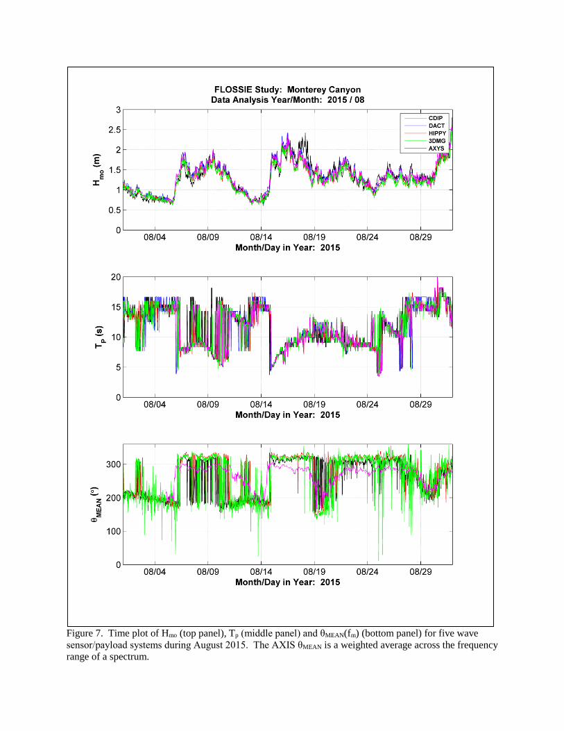
Figure 7. Time plot of Hmo (top panel), Tp (middle panel) and θMEAN(fm) (bottom panel) for five wave

sensor/payload systems during August 2015. The AXIS θMEAN is a weighted average across the frequency

range of a spectrum.

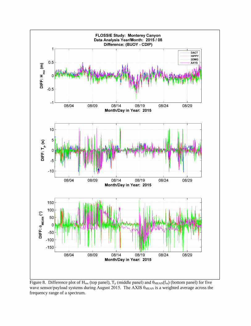
Figure 8. Difference plot of Hmo (top panel), Tp (middle panel) and θMEAN(fm) (bottom panel) for five

wave sensor/payload systems during August 2015. The AXIS θMEAN is a weighted average across the

frequency range of a spectrum.

Improved integral wave parameter evaluations are planned in the future where the First-5 Fourier

coefficients are used to construct S(f,θ) estimates using the Maximum Entropy Method (Lygre and

Krogstad, 1986) and computing directional estimates of θMEAN(fm) for the AXYS data as well as weighted

averages θMEAN for the other three directional measurement platforms. This evaluation will be expanded

to the higher order moments in the directional wave properties beyond the first moment: θMEAN, to the

second moment defined by the directional spread, the third and fourth moment defined by the skewness

and kurtosis, respectively, (O’Reilly et al., 1996).

It was shown the Tp property will be highly variable in a mixed wind-sea, swell environment. Other

definitions can be used for Tp, such as the first moment wave period, the inverse first moment, the Rice5

average wave period �̅�2 = 2𝜋√𝑚0

𝑚2 where m0 and m2 are the zeroth and second moments of the frequency

spectra given by:

𝑚0 = ∫ 𝑆(𝑓)𝑑𝑓

∞

0

(8)

and

𝑚2 = ∫ 𝑓2 ∙ 𝑆(𝑓)𝑑𝑓

∞

0

(9)

Testing for differences of integral wave parameters from various platforms are important, however results

from these evaluations can mask larger errors in the frequency range of a spectrum. The Hmo is an

integral wave parameter calculated from integrating the energy density spectrum (S(f), or C11) over the

entire operational range of frequencies. If the integration of a spectrum is performed over discrete

frequency ranges and compared there could regions where the there are positive biases and alternate

regions containing negative biases. WaveEval Tools (Jensen et al. 2011) dissects the magnitude of the

energy, and the directional moments: mean wave direction, spread, skewness and kurtosis for each

discrete frequency band at a time interval. The two sets of data are then evaluated in the form of

graphical products. WaveEval Tools requires at a minimum of three months of data to adequately

perform the analysis. Hence, this evaluation will have to wait until more data are recovered. The power

and usefulness of this tool will provide insights into where two data sets are similar and where they differ

relative to magnitude in energy and discrete frequency.

SUMMARY AND CONCLUSIONS

Three years have transpired from the initial thoughts of the Field Laboratory for Ocean Sea State

Investigation and Experimentation (FLOSSIE). The ability to house a suite of historical sensor and

payloads from NDBC and EC in a single hull, deploy it in an area containing other wave measurements

platforms and start to recover data from these systems became a reality in July 2015.

The motivation of FLOSSIE was threefold. First it will provide an opportunity to investigate the

similarities and/or differences in historical changes to sensor/payload packages used for nearly 40-years

in 6N buoys. Second is to compare the two North American wave measurement systems and evaluate the

data sets to altimeter wave estimates. Third and more important to EC is to determine the accuracy in

directional wave estimates from NOMAD 6N hull systems. NDBC will be decommissioning all 6N buoy

systems in the near future despite nearly 20- to 40-years of near continuous wave measurements taken

from many of the now operational buoys.

5 Historically the Rice average period was used by NDBC and named in his behalf.

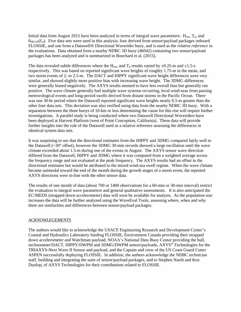
Initial data from August 2015 have been analyzed in terms of integral wave parameters: Hmo, Tp, and

θMEAN(fm). Five data sets were used in this analysis; four derived from sensor/payload packages onboard

FLOSSIE, and one from a Datawell® Directional Waverider buoy, and is used as the relative reference in

the evaluations. Data obtained from a nearby NDBC 3D buoy (46042) containing two sensor/payload

packages has been analyzed and is summarized in Bouchard et al. (2015).

The data revealed subtle differences where the Hmo, and Tp results varied by ±0.25-m and ±1.5-s

respectively. This was based on reported significant wave heights of roughly 1.75-m in the mean, and

two storm events of 2- to 2.5-m. The DACT and HIPPY significant wave height differences were very

similar, and showed slightly more positive bias with increasing wave height. The 3DMG differences

were generally biased negatively. The AXYS results seemed to have less overall bias but generally ran

positive. The wave climate generally had multiple wave systems occurring, local wind-seas from passing

meteorological events and long-period swells derived from distant storms in the Pacific Ocean. There

was one 30-hr period where the Datawell reported significant wave heights nearly 0.5-m greater than the

other four data sets. This deviation was also verified using data from the nearby NDBC 3D buoy. With a

separation between the three buoys of 10-km or less determining the cause for this rise will require further

investigations. A parallel study is being conducted where two Datawell Directional Waveriders have

been deployed at Harvest Platform (west of Point Conception, California). These data will provide

further insights into the role of the Datawell used as a relative reference assessing the differences in

identical system data sets.

It was surprising to see that the directional estimates from the HIPPY and 3DMG compared fairly well to

the Datawell (~30° offset), however the 3DMG 30-min records showed a large oscillation until the wave

climate exceeded about 1.5-m during one of the events in August. The AXYS sensor wave direction

differed from the Datawell, HIPPY and 3DMG where it was computed from a weighted average across

the frequency range and not evaluated at the peak frequency. The AXYS results had an offset in the

directional estimates but would be attributed to the mixed wind-sea swell regime. When the wave climate

became unimodal toward the end of the month during the growth stages of a storm event, the reported

AXYS directions were in-line with the other sensor data.

The results of one month of data (about 700 or 1400 observations for a 60-min or 30-min interval) restrict

the evaluation to integral wave parameters and general qualitative assessments. It is also anticipated the

EC/MEDS (strapped down accelerometer) data will soon be available for analysis. As the population size

increases the data will be further analyzed using the WaveEval Tools, assessing where, when and why

there are similarities and differences between sensor/payload packages.

ACKNOWLEGEMENTS

The authors would like to acknowledge the USACE Engineering Research and Development Center’s

Coastal and Hydraulics Laboratory funding FLOSSIE, Environment Canada providing their strapped

down accelerometer and Watchman payload, NOAA’s National Data Buoy Center providing the hull,

inclinometer/DACT, HIPPY/DWPM and 3DMG/DWPM sensor/payloads, AXYS® Technologies for the

TRIAXYS-Next Wave II Sensor and payload, and the Captain and crew of the US Coast Guard Cutter

ASPEN successfully deploying FLOSSIE. In addition, the authors acknowledge the NDBC technician

staff, building and integrating the suite of sensor/payload packages, and to Stephen Naeth and Ken

Dunlop, of AXYS Technologies for their contributions related to FLOSSIE.

REFERENCES

Alliance for Coastal Technologies (2012). Waves measurement systems test and evaluation protocols,

[UMCESCBL] 12-028, (http://www.act-

us.info/Download/Workshops/2012/USFUM_Wave_Measurement/ ).

Allan, J. C. and P.D. Komar, (2000). Are ocean wave heights increasing in the eastern North Pacific?

EOS, Trans. American Geophysical Union, 47, 561-567.

Bouchard, R. H., R.E. Riley and W. McCall, (2015-in preparation). Long-term intercomparison between

a Datawell wave buoy and an NDBC directional wave buoy: part 1: bulk sea state parameters, 14th

International Workshop on Wave Hindcasting and Forecasting, 9-13 November 2015, Key West Florida.

Collins III, C.O., B. Jund, R.J. Ramos, W.M. Drennan and H.C. Graber, (2014). Wave measurement

intercomparison and platform evauation during the ITOP (2010) experiment, Journal of Atmospheric and

Ocean Technology, Vol. 31, 2310-2329.

Durrant, T.H, D.J.M. Greenslade, and I. Simmonds, (2009). Validation of Jason-1 and Envisat remotely

sensed wave heights, Journal of Atmospheric and Ocean Technology, Vol. 26, 124-134.

Frigaard, P, Helm-Petersen, J, Klopman, G, Standsberg, CT, Benoit, M, Briggs, MJ, Miles, M, Santas, J,

Schäffer, HA & Hawkes, PJ (1997), 'IAHR List of Sea Parameters: an update for multidirectional waves'.

in Mansard, Etienne (ed.), Proceedings of the 27th IAHR Congress, San Francisco, 10-15 August 1997:

IAHR Seminar : Multidirectional Waves and their Interaction with Structures. Canadian Government

Publishing, pp.15-24.

Gemmrich, J., B. Thomas, and R. Bouchard (2011). Observational changes and trends in the Pacific

wave records, Geophy. Res. Letters. Vol 38, L22601.

Integrated Ocean Observing System (2009). A National Operational Wave Observation Plan,

(http://www.ioos.gov/library/wave_plan_final_03122009.pdf.

Jensen, R.E., V.R. Swail, B. Lee and W.A. O’Reilly, (2011). Wave measurement evaluation and

testing,12th International Workshop on Wave Hindcasting and Forecasting, 30 October-4 November

2011,Kohala Coast, Hawaii, (http://www.waveworkshop.org/12thWaves/index.htm ).

Luther, M.E., G. Meadows, E. Buckley, S.A. Gilbert, H. Purcell and M.N. Tamburri, (2013). Verification

of wave measurement systems, Marine Technology Society Journal, Vol 47, No. 5, 104-116.

Lygre. A. and H.E. Krogstad, (1986). Maximum entropy estimation of he directional distribution in

ocean wave spectra, J. Phys. Ocean., 16, 2052-2060.

MacIsaac, C. and S. Naeth, (2013). TRIAXYS next wave II directional wave sensor: the evolution of

wave measurements , http://axystechnologies.com/wp-content/uploads/2013/11/TRIAXYS-Next-Wave-

II-The-Evolution-of-Wave-Sensor.pdf .

Menendez, M., Mendez, F.J., Losada, I., Graham, N.E.,(2008). Variability of extreme wave heights in the

northeast Pacific Ocean based on buoy measurements. Geophysical Research Letters 35, L22607.

doi:10.1029/2008GL035394.

NDBC (1996). NDBC Technical Document 96-01, Nondirectional and Directional Wave Data Analysis

Procedures, National Data Buoy Center, Stennis Space Center, MS, 43 pp.

(http://www.ndbc.noaa.gov/wavemeas.pdf)

NDBC (2009). NDBC Technical Document 09-02, Handbook of Automated Data Quality Control Checks

and Procedures, National Data Buoy Center, Stennis Space Center, MS, 78 pp.

(http://www.ndbc.noaa.gov/NDBCHandbookofAutomatedDataQualityControl2009.pdf)

O’Reilly, W.C., T.H.C. Herbers, R.J. Seymour, and R.T. Guza, (1996). A comparison of directional buoy

and fixed platform measurements of Pacific swell, . J. Atmos. Oceanic Technol., 13, 231-238.

Riley, R., C.-C. Teng, R. Bouchard, R. Dinoso and T. Mettlach, (2011). Enhancements to NDBC’s

digital directional wave module, Proceedings of MTS/IEEE Oceans 2011 Conference, Kona, Hawaii,

September 2011.

Ruggerio, P., J.C. Allan, and P.D. Komar, (2010). Increasing wave heights, and extreme-value

projections: the wave climate of the U.S. Pacific Northwest, Coastal Engineering, 57(5), 539-552.

Skey, S.G.P., K. Berger-North and V.R. Swail, (1995). Detained measurements of winds and waves in

high seastates from a moored NOMAD weather buoy, 4th International Workshop on Wave Hindcasting

and Forecasting, 16-20 October 1995, Banff, Alberta Canada, 213-223.

Swail, V., R.E. Jensen, B. Lee, J. Turton, J. Thomas, S. Gulev, M. Yelland, P. Etala, D. Meldrum, W.

Birkemeier, W. Burnett, and G. Warren (2009). Wave measurements, needs and developments for the

next decade, Proceedings of OceanObs’09, Vol. 2 II-1-87, 999-1008.

Timpe, G.L., and N. Van de Voorde, (1995). NOMAD buoys: an overview of forty years of use,

OCEANS’95 MTS/IEEE, Challenges of Our Changing Global Environment, 9-12 October 1995, San

Diego, CA, Vol. 1, 309-315.

Van Straten, F.W (1966). Weather or Not, Dodd, Mead & Company, New York, NY, 252 pp.

WMO, (1995), “FM65 –XI WAVEOB”, World Meteorological Organziation (WMO) Manual on Codes,

International Codes Vol.I.1, Part A – Alphanumeric Codes, WMO-No.306, pp. 129-132.