ORNL/TM-2011/419

Field Measurements at Rivers and Tidal Current Sites for Hydrokinetic Energy Development: Best Practices Manual

September 2011 Prepared by Vincent S. Neary, Ph.D., P.E. 1 Budi Gunawan, Ph.D. 1 Marshall C. Richmond, Ph.D. P.E. 2 Vibhav Durgesh, Ph.D. 2 Brian Polagye, Ph.D. 3 Jim Thomson, Ph.D. 3 Marian Muste, Ph.D. 4 Arnie Fontaine, Ph.D. 5

1 Oak Ridge National Laboratory 2 Pacific Northwest National Laboratory 3 Northwest National Marine Renewable Energy Center, University of Washington 4 IIHR—Hydroscience & Engineering, University of Iowa 5 Applied Research Laboratory, Penn State University

DOCUMENT AVAILABILITY Reports produced after January 1, 1996, are generally available free via the U.S. Department of Energy (DOE) Information Bridge. Web site http://www.osti.gov/bridge Reports produced before January 1, 1996, may be purchased by members of the public from the following source. National Technical Information Service 5285 Port Royal Road Springfield, VA 22161 Telephone 703-605-6000 (1-800-553-6847) TDD 703-487-4639 Fax 703-605-6900 E-mail info@ntis.gov Web site http://www.ntis.gov/support/ordernowabout.htm Reports are available to DOE employees, DOE contractors, Energy Technology Data Exchange (ETDE) representatives, and International Nuclear Information System (INIS) representatives from the following source. Office of Scientific and Technical Information P.O. Box 62 Oak Ridge, TN 37831 Telephone 865-576-8401 Fax 865-576-5728 E-mail reports@osti.gov Web site http://www.osti.gov/contact.html

This report was prepared as an account of work sponsored by an agency of the United States Government. Neither the United States Government nor any agency thereof, nor any of their employees, makes any warranty, express or implied, or assumes any legal liability or responsibility for the accuracy, completeness, or usefulness of any information, apparatus, product, or process disclosed, or represents that its use would not infringe privately owned rights. Reference herein to any specific commercial product, process, or service by trade name, trademark, manufacturer, or otherwise, does not necessarily constitute or imply its endorsement, recommendation, or favoring by the United States Government or any agency thereof. The views and opinions of authors expressed herein do not necessarily state or reflect those of the United States Government or any agency thereof.

ORNL/TM-2011/419

Environmental Science Division

FIELD MEASUREMENTS AT RIVERS AND TIDAL CURRENT SITES FOR HYDROKINETIC ENERGY DEVELOPMENT: BEST PRACTICES

MANUAL

Vincent S. Neary, Ph.D., P.E. Budi Gunawan, Ph.D.

Marshall C. Richmond, Ph.D., P.E. Vibhav Durgesh, Ph.D. Brian Polagye, Ph.D. Jim Thomson, Ph.D. Marian Muste, Ph.D. Arnie Fontaine, Ph.D.

Date Published: September 30, 2011

Prepared by OAK RIDGE NATIONAL LABORATORY

Oak Ridge, Tennessee 37831-6283 managed by

UT-BATTELLE, LLC for the

U.S. DEPARTMENT OF ENERGY under contract DE-AC05-00OR22725

iv

v

CONTENTS

CONTENTS  V 

LIST OF FIGURES  VIII 

LIST OF TABLES  XII 

NOTATION  XIV 

ACKNOWLEDGMENTS  XV 

1.  INTRODUCTION  16 

2.  RIVERS AND TIDAL CHANNELS  18 

2.1 Channel Morphology  18 

2.2 Flow Variability in Rivers  19 

2.3 Tidal Currents and Tidal Variability  20 

2.4 Velocity and Turbulence, Distributions and Magnitudes  22 

2.5 Velocity and Turbulence Measurements at Tidal Energy Sites  26 

2.6 Effects of Depth Variability in Rivers  28 

2.7 Waves  28 

3.  PROPERTIES TO BE MEASURED  29 

3.1 Study Reach Bathymetry  29 

3.2 Fluvial Hydraulic Properties  30 3.2.1 Sediment Properties  30 3.2.2 Bed Forms  30 3.2.3 Substrate Composition  32 3.2.4 Substrate Stability  33 

3.3 Temperature, density and viscosity  33 

3.4 Turbidity  34 

3.5 Flow Field Properties  34 3.5.1 Bulk Flow and Section Geometry Properties  35 3.5.2 Mean (Reynolds or time‐averaged) Flow Properties  36 

3.5.2.1 Mean (Time‐averaged) Velocity  37 

vi

3.5.2.2 Turbulence Intensity and Reynolds Stresses  38 

4.  INSTRUMENTATION, DEPLOYMENT AND MEASUREMENT PROTOCOLS  42 

4.1 Bathymetric Mapping with Echosounders  42 

4.2 Sediment Properties, Bed Forms, Substrate Composition, Roughness and Substrate Stability  42 4.2.1 Bed Forms  42 4.2.2 Substrate Core and Grab Sampling Equipment and Methods  43 

4.3 Temperature and Pressure  47 

4.4 Turbidity and Conductivity  48 

4.5 Mean (Reynolds or time‐averaged) Flow Properties  48 4.5.1 Velocity Measurements using Acoustic Methods  48 4.5.2 ADV Instrument Details  51 4.5.3 ADCP Instrument Details  52 4.5.4 ADV and ADCP Deployment Methods  55 4.5.5 ADV Error and Signal Processing Methods  59 

4.5.5.1 Sources of Error  59 4.5.5.2 Protocols for Reducing Error  61 4.5.5.3 Methods for Error Removal  62 

4.5.6 ADCP Data Quality Control and Post‐processing  64 4.5.6.1 Preventing Interference between Acoustic Instruments  64 4.5.6.2 Correcting for Clock Drift  65 4.5.6.3 Measurements near Boundaries  65 4.5.6.4 Velocity Quality Control  67 4.5.6.5 Lack of Scatterers issue  67 4.5.6.6 Transducers Ringing  67 4.5.6.7 Velocity Ambiguity  67 4.5.6.8 Moving‐bed Condition  67 4.5.6.9 Air bubbles  68 4.5.6.10 Temporal averaging  68 4.5.6.11 Spatial averaging  69 4.5.6.12 Histogram inspection  70 

4.6 ADV and ADCP Measurements at Marrowstone Island, WA  71 4.6.1 Mean Velocities and Power Densities  71 4.6.2 Velocity & power density histogram  73 4.6.3 Turbulence Intensities  75 4.6.4 TKE Dissipation and Power Spectra  75 4.6.5 Flow Directionality  77 

4.7 Waves  78 

5.  CONCLUSIONS  79 

REFERENCES  82 

   

vii

viii

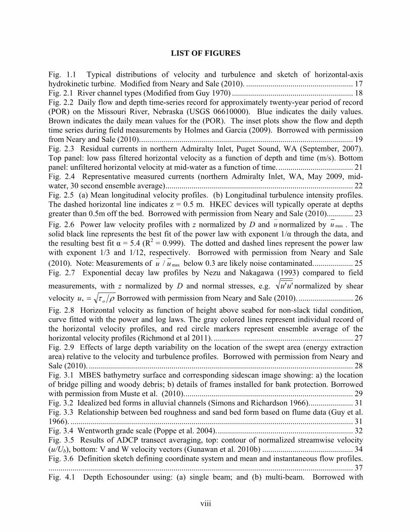
LIST OF FIGURES

Fig. 1.1 Typical distributions of velocity and turbulence and sketch of horizontal-axis hydrokinetic turbine. Modified from Neary and Sale (2010). ..................................................... 17 Fig. 2.1 River channel types (Modified from Guy 1970) ............................................................ 18 Fig. 2.2 Daily flow and depth time-series record for approximately twenty-year period of record (POR) on the Missouri River, Nebraska (USGS 06610000). Blue indicates the daily values. Brown indicates the daily mean values for the (POR). The inset plots show the flow and depth time series during field measurements by Holmes and Garcia (2009). Borrowed with permission from Neary and Sale (2010). ......................................................................................................... 19 Fig. 2.3 Residual currents in northern Admiralty Inlet, Puget Sound, WA (September, 2007). Top panel: low pass filtered horizontal velocity as a function of depth and time (m/s). Bottom panel: unfiltered horizontal velocity at mid-water as a function of time. ..................................... 21 Fig. 2.4 Representative measured currents (northern Admiralty Inlet, WA, May 2009, mid-water, 30 second ensemble average) ............................................................................................. 22 Fig. 2.5 (a) Mean longitudinal velocity profiles. (b) Longitudinal turbulence intensity profiles. The dashed horizontal line indicates z = 0.5 m. HKEC devices will typically operate at depths greater than 0.5m off the bed. Borrowed with permission from Neary and Sale (2010). ............ 23 Fig. 2.6 Power law velocity profiles with z normalized by D and normalized by . The solid black line represents the best fit of the power law with exponent 1/α through the data, and the resulting best fit α = 5.4 (R2 = 0.999). The dotted and dashed lines represent the power law with exponent 1/3 and 1/12, respectively. Borrowed with permission from Neary and Sale (2010). Note: Measurements of / below 0.3 are likely noise contaminated. ................... 25 Fig. 2.7 Exponential decay law profiles by Nezu and Nakagawa (1993) compared to field

measurements, with z normalized by D and normal stresses, e.g. normalized by shear

velocity Borrowed with permission from Neary and Sale (2010). ........................... 26 

Fig. 2.8 Horizontal velocity as function of height above seabed for non-slack tidal condition, curve fitted with the power and log laws. The gray colored lines represent individual record of the horizontal velocity profiles, and red circle markers represent ensemble average of the horizontal velocity profiles (Richmond et al 2011). ..................................................................... 27 Fig. 2.9 Effects of large depth variability on the location of the swept area (energy extraction area) relative to the velocity and turbulence profiles. Borrowed with permission from Neary and Sale (2010). ................................................................................................................................... 28 Fig. 3.1 MBES bathymetry surface and corresponding sidescan image showing: a) the location of bridge pilling and woody debris; b) details of frames installed for bank protection. Borrowed with permission from Muste et al. (2010). ................................................................................... 29 Fig. 3.2 Idealized bed forms in alluvial channels (Simons and Richardson 1966). ..................... 31 Fig. 3.3 Relationship between bed roughness and sand bed form based on flume data (Guy et al. 1966). ............................................................................................................................................ 31 Fig. 3.4 Wentworth grade scale (Poppe et al. 2004). ................................................................... 32 Fig. 3.5 Results of ADCP transect averaging, top: contour of normalized streamwise velocity (u/Ub), bottom: V and W velocity vectors (Gunawan et al. 2010b) ............................................. 34 Fig. 3.6 Definition sketch defining coordinate system and mean and instantaneous flow profiles........................................................................................................................................................ 37 Fig. 4.1 Depth Echosounder using: (a) single beam; and (b) multi-beam. Borrowed with

u maxu

u maxu

''uu

ou *

ix

permission from Muste et al. (2010). ........................................................................................... 42 Fig. 4.2 Ponar-type grab samplers (Rickly Hydrological Company 2010). ................................ 43 Fig. 4.3 Deployment of 3-inch VibeCore-D Sampler for deep water sediment sampling. VibeCore Brochure 2008. ............................................................................................................. 45 Fig. 4.4 Mechanical sieve shaker with five sieves and bottom pan. ............................................ 46 Fig. 4.5 Bed sediments separate with standard 12” mechanical sieve kit (From Neary 2009). .. 46 Fig. 4.6 Cumulative particle size distribution to determine surface roughness of gravel stream channel (Neary 2009). ................................................................................................................... 47 Fig. 4.7 Salinity measurements obtained from northern Admiralty Inlet, WA with a Seabird 16plus v2 showing the effect of biofouling in the salinity step change during instrument turn-around. .......................................................................................................................................... 48 Fig. 4.8 Acoustic Doppler velocity instruments: a) illustration of the Doppler effect; b) ADV for point measurements; c) Horizontal ADCP for instantaneous horizontal velocity profiles; d) ADCP for instantaneous measurement of vertical velocity profiles. From Muste et al. (2010). .. 49 Fig. 4.9 Photograph of Sontek 10MHz ADV(left) and an illustration of Nortek Vectrino ADV probe head with four receive beams (right) (Adapted from Sontek 2011 and Nortek 2009). ...... 51 Fig. 4.10 Different types of ADCP beam configurations (RDI 2011) ......................................... 52 Fig. 4.11 Beam velocity components at a depth cell (RDI 1996). ............................................... 53 Fig. 4.12 Resultants of east-west and north-south velocities (RDI 1996). .................................. 53 Fig. 4.13 Schematic of four beam ADCP showing typical sampling volume. ............................ 54 Fig. 4.14 Comparison of ADV and ADCP data in the middle of a meandering river cross-section: (a) time allocation of measurements, (b) streamwise velocity, (c) lateral velocity, (d) vertical velocity (Gunawan et al. 2008). ....................................................................................... 55 Fig. 4.15 Stationary tripod deployed ADV and ADCP used for Marrowstone Island, WA deployment (Richmond et al. 2010). ............................................................................................. 56 Fig. 4.16 Cable-deployed ADV (CDADV) with sounding weight (Photograph courtesy of Bob Holmes, USGS, 2010)................................................................................................................... 56 Fig. 4.17 ADCP deployment methods: (a) mooring, (b) mounted, (c) underwater vehicle, (d) remote controlled boat (RDI 2011b; Muller and Wagner 2009). ................................................. 57 Fig. 4.18 Two views of shipboard ADCP side-swing mount on a 30-meter (95-foot) vessel (Simpson 2001). ............................................................................................................................ 58 Fig. 4.19 Schematic view of the ADCP cableway system used in Gunawan 2010 (top); ........... 58 Fig. 4.20 ADCP cableway systems for flow measurement in inbank and overbank flow conditions at River Teme, UK (Gunawan, unpublished data). ..................................................... 59 Fig. 4.21 Typical auto-spectra for longitudinal velocity component and white noise level calculated from measured Doppler Noise (Nikora and Goring 1998) .......................................... 61 Fig. 4.22 Shipboard ADCP measurements of currents (m/s) contaminated by cross-talk (top) and post-processed with most interference removed (bottom). ........................................................... 65 Fig. 4.23 Contamination of horizontal current velocity within 4m of the free surface for a bottom-mounted ADCP (Polagye, unpublished data) .................................................................. 66 Fig. 4.24 Depth averaged streamwise velocity and bottom profile obtained using stationary (vertical) and moving-boat (transverse) methods at a straight section of the River Blackwater, UK (Gunawan 2010). .................................................................................................................... 70 Fig. 4.25 Difference between Ud values obtained from ADCP stationary measurements and ADCP transect averaging results at two cross sections (Gunawan 2010). ................................... 70 Fig. 4.26 Mean velocities from ADV measurements at Marrowstone Island site. ...................... 72 

x

Fig. 4.27 Mean horizontal velocities from ADV measurements at Marrowstone Island site. ..... 73 Fig. 4.28 Horizontal velocities, along with directions, from ADCP measurements at Marrowstone Island site. ............................................................................................................... 73 Fig. 4.29 Histogram of u-component of velocity from ADV measurements at Marrowstone Island site. ..................................................................................................................................... 74 Fig. 4.30 Histogram of v-component of velocity from ADV measurements at Marrowstone Island site. ..................................................................................................................................... 74 Fig. 4.31 Histogram of horizontal component of velocity from ADV measurements at Marrowstone Island site. ............................................................................................................... 74 Fig. 4.32 Histogram of power density calculated from ADV measurements at Marrowstone Island site. ..................................................................................................................................... 74 Fig. 4.33 Typical spectra for all components of velocity, from ADV measurements, for non-slack period at Marrowstone Island site. ....................................................................................... 77 Fig. 4.34 Typical spectra for all components of velocity, from ADV measurements, for slack period at Marrowstone Island site. ................................................................................................ 77 Fig. 4.35 Average spectra for all components of velocity, from ADV measurements, for non-slack period at Marrowstone Island site. ....................................................................................... 77 Fig. 4.36 Average spectra, for all components, from ADV measurements, for slack period at Marrowstone Island site. ............................................................................................................... 77 Fig. 4.37 Scatter plot of the horizontal components of velocity from ADCP measurements: (a) at base, (b) at hub, and (c) at top of an MHK device. ....................................................................... 78 Fig. 5.1 Two input single output system. ..................................................................................... 80 Fig. 5.2 Add-on devices for suppression of vortex-induced vibration of cylinders (a) helical strake; (b) shroud; (c) axial slats; (d) streamlined fairing; (e) splitter; (f) ribboned cable; (g) pivoted guiding vane; (h) spoiler plates. (Dalton, C., U. Houston).Error! Bookmark not defined. 

xi

xii

LIST OF TABLES

Table 3.1 Bulk flow properties of reviewed open channel flow data ........................................... 36 Table 4.1 Minimum averaging time for ADCP stationary measurement in rivers suggested by different researchers. ..................................................................................................................... 68 Table 4.2 ADV and ADCP statistics summary table. .................................................................. 75 

xiii

xiv

NOTATION

NOTATION

= maximum longitudinal time-averaged velocity in vertical profile, m s-1

= shear velocity, , m s-1

τo = bed shear stress, N m-2

κ = Von Kármán constant

ks = characteristic roughness length scale, m

g = gravitational acceleration constant, m s-2

P = wetted perimeter, m

A = flow section area, m2 R = hydraulic radius, , m

S = water slope

Q = discharge, m3 s-1

Qm = mean annual discharge, m3 s-1

W = local channel width, m

D = local water depth, m

Davg = cross sectional average water depth, m

R = Reynolds number,  

F = Froude number,  

UDavg = depth averaged longitudinal velocity, m s-1 u,v,w = instantaneous longitudinal, lateral, and vertical velocities, m s-1

= time-averaged longitudinal, lateral, and vertical velocities, m s-1 u',v’,w’ = instantaneous longitudinal, lateral, and vertical fluctuating velocities, m s-1

, , = standard deviation of the longitudinal, lateral, and vertical velocities, m s-1

x, y , z = longitudinal, lateral, and vertical coordinate distance, m

= body force per unit volume of fluid, N m-3 p = isotropic hydrostatic pressure force, N m-2 ρ = fluid density, kg m-3 v = kinematic viscosity, m2 s-1

µ = dynamic viscosity, N s m-1

α = power law exponent (1/α)

maxu

*u o

PA

wvu ,,

''uu ''vv ''ww

f

xv

ACKNOWLEDGMENTS

The authors thank DOE/EERE for supporting the development of this manual under CPS Project No. 20689, CPS Agreement Nos. 20065 and 20070.

16

1. INTRODUCTION Current energy conversion technologies are a class of marine and hydrokinetic (MHK) technologies that convert kinetic energy of river, tidal or ocean currents to generate electricity. These technologies are at early stages of development compared to other renewable technologies, such as wind turbines, and require the Department of Energy’s support to accelerate their advancement to the market place. Hence, the Wind and Water Power Program (WWP), administered by the U.S. Department of Energy’s Energy Efficiency and Renewable Energy Office, has implemented a research and development program to estimate the baseline LCoE for these technologies, with the goal of reducing it to $0.07/kW-h by 2030. Accurate estimates of LCoE for MHK devices are therefore needed to compare with conventional and other renewable energy technologies and to identify key cost drivers and cost reduction strategies. As part of this overarching goal to reduce LCoE the WWP has adopted a technology readiness level (TRL) framework to facilitate the advancement of hydrokinetic energy conversion (MHK) technologies. Although the majority of proposed MHK machines are still in the conceptual and scaled prototype stage of design, many have progressed beyond the proof of concept stages and are now ready for full scale field testing and deployment. Best practice guidelines and protocols are needed for collecting field measurements needed for these tests and deployments to ensure the data collected is consistent for comparison among different technologies and tests. The WWP has also supported hydrokinetic energy resource assessments to characterize and quantify the theoretical, technical and practical energy available in the US for each of the MHK resource types, including separate resource assessments for river, tidal and ocean currents. These resource assessments, however, are only at a reconnaissance level with power densities averaged over model grid cells on the order of 300-500m (e.g. Defne et al 2011). More refined field measurements at the development site are required to assess and characterize the resource at the scale of the individual MHK machine and MHK machine array. For individual MHK machine design, measurements over the energy extraction plane (EEP) are needed to inform machine design and to establish reference hydrodynamics for environmental impact studies. As illustrated in Fig. 1.1, MHK developers would benefit from measurements of mean velocity and turbulence at their deployment sites; particularly over EEP of their device for component design and estimation of performance, annual energy production, and LCoE. These measurements require well designed deployments of state-of-the-art acoustic instruments, including acoustic Doppler current profilers (ADCP) and acoustic Doppler velocimeters (ADV).

In this report, existing data collection techniques and protocols for characterizing open channel flows are reviewed and refined to further address the needs of the MHK industry. The report provides an overview of the hydrodynamics of river and tidal channels, and the working principles of modern acoustic instrumentation, including best practices in remote sensing methods that can be applied to hydrokinetic energy site characterization. Emphasis is placed upon acoustic Doppler velocimeter (ADV) and acoustic-Doppler current profiler (ADCP) instruments, as these represent the most practical and economical tools for use in the MHK

17

industry. Incorporating the best practices as found in the literature, including the parameters to be measured, the instruments to be deployed, the instrument deployment strategy, and data post-processing techniques. The data collected from this procedure aims to inform the hydro-mechanical design of MHK systems with respect to energy generation and structural loading, as well as provide reference hydrodynamics for environmental impact studies. The standard metrics and protocols defined herein can be utilized to guide field experiments with MHK systems.

Fig. 1.1 Typical distributions of velocity and turbulence and sketch of horizontal-axis hydrokinetic turbine. Modified from Neary and Sale (2010).

18

2. RIVERS AND TIDAL CHANNELS

2.1 CHANNEL MORPHOLOGY

The morphology of natural rivers and tidal channels is complex compared to engineered channels, which can include power, irrigation and drainage canals. Measurements of bathymetry and hydrodynamics are therefore more challenging. Natural channels typically have mobile boundaries composed of substrates ranging in sizes from fine clay, with a median grain size of half a micron, to very large boulders with median grain sizes that equal or exceed 4 meters. Four basic classes of natural channels are illustrated in Fig. 2.1 based on the channel slope or water discharge and the median grain size of the bed substrates: sinuous uniform (canaliform), sinuous point bar, point-bar braided, and bar- or island braided (including anabranched). Historically, large braided and anabranched channels have been channelized in most of the United States, with the exception of Alaska. Sinuous braided, point bar, and canaliform channels are therefore anticipated to be the most common river morphologies for MHK machine and array deployment.

Fig. 2.1 River channel types (Modified from Guy 1970)

Unregulated and regulated rivers and tidal channels are rarely uniform along their reaches. Natural channels are rarely straight over twenty channel widths and are nonuniform in plan, profile, and section. This results in super-elevation of the water surface around bends that can generate strong secondary circulation, mixed water surface profiles, and convective acceleration and deceleration of the bulk velocity. Channel geometry, roughness, mean-section depth and bulk velocity typically change along the longitudinal direction. In addition to challenges in characterizing the variations of bulk (section averaged) flow properties, the local mean flow properties of rivers and tidal channels can be highly three-dimensional as a result of variations in river alignment and vortex shedding from in-stream structures and surface vessels. Pressure gradients associated with nonuniform surface profiles cause significant departures in the wake

19

region. Wind shear on the water surface also can cause significant departures from semi-theoretical models that estimate mean velocity and Reynolds stress profiles. Bed sediments, grain and form roughness can also vary considerably among different channels and along a channel reach. Adding to this already complex morphology and roughness are in-stream structures and surface vessels that produce surface wakes, vortex shedding, and increased turbulence in the wakes. In-stream structures include bridge piers, docks, alluvial sand dunes (Best et al. 2010), medium and large boulders greater than 500 mm in diameter (Crowder and Diplas 2000), boulder clusters (Tritico and Hotchkiss 2005; Lacey and Roy 2008), large woody debris, and aquatic vegetation (Neary et al., In Review). Barge and boat traffic also generate surface wakes, vortex shedding and turbulence (Bhowmik et al. 1982). The above morphological complexities result in nonuniform flows with a wide range of bulk flow conditions, eddy frequencies and scales and velocity fluctuations.

2.2 FLOW VARIABILITY IN RIVERS

Classical models assume steady uniform flow, but unregulated rivers exhibit great variability of discharge and depth over time scales varying from hours to days depending on the size of the drainage basin. The discharge of regulated rivers, such as tailwaters below hydropower dams, can change within minutes, but exhibit less depth and flow variability than regulated rivers. Fig. 2.2 shows daily discharge and stage data on the Missouri River for an approximately twenty year period. The discharge at this site varies over three orders of magnitude, and the stage varies from approximately 1 to 30 m.

Fig. 2.2 Daily flow and depth time-series record for approximately twenty-year period of record

(POR) on the Missouri River, Nebraska (USGS 06610000). Blue indicates the daily values. Brown indicates the daily mean values for the (POR). The inset plots show the flow and depth

time series during field measurements by Holmes and Garcia (2009). Borrowed with permission from Neary and Sale (2010).

20

Rivers can have extreme variations in flow and stage, and measurements on the order of several decades are typically required to obtain meaningful statistics on the flow variability. It is impractical for instrument deployments to span the return periods found in rivers due to instrument limitations and prohibitive costs. Alternatively, classical models developed from laboratory experiments to describe velocity and turbulence profiles in open channel flows may be used as a first approximation of river hydrokinetic resources (Neary and Sale 2010). These classical models, however, need more extensive validation for large river flows, particularly for the transverse and vertical components of the normal Reynolds stresses (Nezu and Nakagawa 1993). These models include the power and logarithmic laws for the vertical mean velocity profile of a flat plate turbulent boundary layer flow and exponential decay models developed by Nezu and Nakagawa (1993) for normal Reynolds stresses of depth-limited boundary shear flows in open channel flumes.

2.3 TIDAL CURRENTS AND TIDAL VARIABILITY

Tidal currents are primarily derived from variations in tidal elevation, which are in turn derived from the gravitational forcing of the moon and sun on the earth's oceans. While currents are quite weak in the open ocean, in coastal environments relative constrictions can increase peak currents to 3-5 m/s (6-10 knots). At sites of hydrokinetic interest, currents are generally aligned to a principal axis on ebb (water flowing inwards) and flood (water flowing outwards). However, asymmetries between the strength and direction of ebb and flood are common and symmetric, rectilinear currents are an exceptional case. The tidal regimes at sites of practical importance for power generation are either semidiurnal (two ebb and flood tides of equal strength each lunar day) or mixed, mainly semidiurnal (two ebb and flood tides each lunar day with one cycle considerably strong than the other). In addition to gravitational forcing, the site-specific signals from estuarine circulation (e.g., stratification), wind, waves, and bathymetric effects may be present in measured currents. The time scales for tidal variability in the mean flow are fundamentally different than for rivers. Tidal currents vary continually in response to the lunar and solar gravitational interaction with the earth's oceans. An idealized model for tidal currents consists of a series of superimposed sinusoids corresponding to the relative position and orientation of the celestial bodies:

,

where i is a particular constituent and u, ω, and φ are its associated amplitude, period, and phase. As described above, the primary modulation is over the 24-hour lunar day, but longer turn modulations are also present, the 14.8-day neap-spring cycle being the most pronounced. During spring tides, the gravitational forcing from the moon and sun are in phase and currents are strongest. Neap tides occur when the gravitational forcing from these two bodies is out of phase and currents are weakest. In addition to the smoothly varying tidal forcing, measured currents also include residual currents associated with non-tidal variability at two primary time scales. Seasonally, stratification between salt water and fresh water in estuaries may drive residual currents. While

N

iiii tutu

1

sin

21

these play a critical role in estuarine ecology, they may be a second order effect for hydrokinetic performance evaluation. For example, at sites in Puget Sound, WA, residual currents vary from approximately -30 cm/s (net outflow at surface) to 30 cm/s (net inflow at seabed) and may be quite weak at the middle of the water column (where tidal energy devices would be most likely to be deployed). An example of this is shown in Fig. 2.3. In comparison, peak tidal currents may exceed 300 cm/s throughout the water column.

Fig. 2.3 Residual currents in northern Admiralty Inlet, Puget Sound, WA (September, 2007). Top panel: low pass filtered horizontal velocity as a function of depth and time (m/s). Bottom

panel: unfiltered horizontal velocity at mid-water as a function of time. Over shorter time scales, tidal currents may depart considerably from the idealization of a smoothly varying sinusoid. An example of this is shown in Fig. 2.4. While tidal currents are dominated by the harmonic forcing of the sun and moon over time periods on the order of a lunar day, shorter term fluctuations may be pronounced. On time scales of longer than several minutes, influences include local bathymetric features, eddies created by headlands or other topographic features, or hydraulic control. These features may be periodic (e.g., secondary peak flood current prior to the true peak), but are not harmonic in the same sense as the tides (Polagye et al. 2010). On time scales shorter than several minutes, higher frequency fluctuations are associated with turbulence at various lengths and time scales (Thomson et al. 2010).

22

Fig. 2.4 Representative measured currents (northern Admiralty Inlet, WA, May 2009, mid-water, 30 second ensemble average)

2.4 VELOCITY AND TURBULENCE, DISTRIBUTIONS AND MAGNITUDES

Over periods of steady or quasi-steady flow, Neary and Sale (2010) showed that vertical profiles of velocity and Reynolds stresses generally follow classical laws if large roughness effects and obstructions that perturb boundary shear flows are absent. Mean longitudinal velocity profiles measured in large rivers are shown in Fig. 2.5a. As expected, the mean velocity is lowest near the channel bottom and increases as it approaches the free water surface z=D. The maximum is usually near the free water surface. Maximum values range from 1 to 4 m/s and depths z from 1 to 35 m for the data reviewed. Given that flow measurements for the Mississippi River by McQuivey (1973) were taken when the flow was well below the mean annual discharge Qm (Table 1), one would expect higher maximum at higher z and flows Q>Qm. The corresponding longitudinal turbulence intensity profiles are shown in Fig. 2.5b. These profiles also follow known trends with an exponential increase from the free water surface to the near wall region. When comparing the velocity and turbulence profiles in Fig. 2.5b, one

observes that the longitudinal turbulence intensity ranges from approximately 0.05 to 0.5

m/s and is usually an order of magnitude less than . The no-slip condition requires that the turbulence intensity and all components of the Reynolds stress tensor are zero at the bottom of a fixed boundary, but field measurements are currently limited within the near wall region, even with state-of-the-art acoustic instruments, and rivers typically have mobile beds with non-zero mean velocity and Reynolds stresses. The minimum and maximum range of elevations for measurements by McQuivey, Holmes and Garcia, Nikora and Smart, and Carling et al. were z/D=0.03-0.91, 0.02-0.96, 0.27-0.93 and 0.06-0.77, respectively.

u

u

u

u

''uuu

23

Fig. 2.5 (a) Mean longitudinal velocity profiles. (b) Longitudinal turbulence intensity profiles. The dashed horizontal line indicates z = 0.5 m. HKEC devices will typically operate at depths

greater than 0.5m off the bed. Borrowed with permission from Neary and Sale (2010).

a) b)

24

Field measurements of non-dimensionalized by with the power law equation

,

are shown in Fig. 2.6. Based on the power law assumption, occurs at the surface (z/D = 1), but the measured data shows that can occur beneath the surface due to wind, wave and three-dimensional flow effects.

The power law exponent was observed by Neary and Sale (2010) to vary from 1/3 to 1/12 between individual profiles, with a best fit value of 1/5.4 through all the data. Variation in the exponent can be attributed to a number of causes, including measurement error, pressure gradients, roughness and three-dimensional flow effects. The significant differences between the exponents would translate into more significant errors in drag and power acting on the energy extraction plane since drag and power are proportional to to the second and third powers.

Field measurements of normal stresses, e.g. , normalized by shear velocity are

compared in Fig. 2.7 with exponential decay models developed by Nezu and Nakagawa (1993) for steady uniform flow in smooth laboratory flumes

These expressions are universal for smooth boundaries between (0.1-0.2)< z/D<0.9, independent

of Reynolds and Froude number, and show that > > . They do not apply near the wall approximately z/D<(0.1 to 0.2) as the no slip condition requires turbulence intensities to decrease from a maximum value to zero at z/D=0. Nor do they apply in the free

surface region above z/D<0.9, where is damped. A peak value of =2.8 is observed in the near-wall region in wall coordinates at z+=17, where (Nezu and

Nakagawa 1993). A peak in was not observed in any of the data reviewed because the measurements were not taken close enough to the bed.

The comparison by Neary and Sale (2010) indicated that field measurements are in reasonable agreement with the exponential decay models developed from laboratory flumes, although there is considerable scatter. Measurement error as well as complex hydrodynamic effects summarized above are possible causes. The measurements by Holmes and Garcia (2008) are the

only known measurements of the normal Reynolds stresses and for large rivers (depths > 1 m and currents > 1m/s). These turbulence measurements are in fair agreement with the exponential decay models, except near the surface where the models underestimate the

u maxu

1

max

D

z

u

u

maxu

maxu

1

u

''uu ou *

Dzuww

Dzuvv

Dzuuu

exp27.1''

exp63.1''

exp30.2''

*

*

*

*'' uuu *'' uvv *'' uww

*'' uww *'' uuu*zuz

*'' uuu

*'' uvv *'' uww

25

data. Field measurements near the free water surface, however, are likely prone to error from wave motion and wind shear effects.

Fig. 2.6 Power law velocity profiles with z normalized by D and normalized by . The

solid black line represents the best fit of the power law with exponent 1/α through the data, and the resulting best fit α = 5.4 (R2 = 0.999). The dotted and dashed lines represent the power law

with exponent 1/3 and 1/12, respectively. Borrowed with permission from Neary and Sale (2010). Note: Measurements of / below 0.3 are likely noise contaminated.

u maxu

u maxu

26

Fig. 2.7 Exponential decay law profiles by Nezu and Nakagawa (1993) compared to field

measurements, with z normalized by D and normal stresses, e.g. normalized by shear

velocity Borrowed with permission from Neary and Sale (2010).

2.5 VELOCITY AND TURBULENCE MEASUREMENTS AT TIDAL ENERGY SITES

For tidal energy sites, the calculation of turbulence intensity (absolute or relative) is complicated by the inherently non-stationary mean flow. Returning to the previous idealization of the tidal cycle, an idealization of mean current velocity of a tidal cycle is a sine wave of given period and amplitude. The time rate of change of velocity is only non-zero at peak flood or peak ebb and at a maximum around slack. If the averaging window over which the mean is calculated is short (e.g., less than a minute), the additional "turbulence" introduced by a non-stationary mean should be small in comparison to the true turbulence. However, an averaging period of this length is not always possible and for averaging periods of greater than a few minutes, the spurious turbulence intensity masks true turbulence over most of the tidal cycle (Polagye and Thomson in

''uu

ou *

(a) (b) (c)

27

preparation). Second, any acoustic measurement of current velocity will contain additional variance associated with Doppler noise. Factors influencing Doppler noise for a single ping include vertical bin size, ADCP frequency, and the ambiguity velocity chosen to prevent phase wrapping. A correction for Doppler noise is presented in Thomson et al. (2010), but assuming that over the averaging window Doppler noise is normally distributed. Depending on the instrument sampling rate, it may not be possible to satisfy both the requirement of an averaging window short enough to prevent a substantially non-stationary mean and an averaging window long enough to ensure normal statistics for Doppler noise. In practice, mean tidal currents show more variability than in the case of an idealized sinusoid, but the complication of a non-stationary mean is analogous. The mean horizontal velocity, at Marrowstone Island, WA study site, calculated from ADCP data (see Richmond et al. 2011) is shown in Fig. 2.8. The averaged velocity data appears to have a good agreement with the log law and, at most of the profile, with the power law. Deviations from the power law are observed near the surface and bed. The log and power law equations used are in the following form:

∗

1

0.4

where ∗ is the flow friction or shear velocity and is the surface roughness length; both are estimated using a nonlinear least square regression fitting.

where is the reference velocity (i.e., horizontal velocity at the hub of MHK devices), z is the height above the seabed, is the height of the hub from the seabed and is the exponent for the power law.

Fig. 2.8 Horizontal velocity as function of height above seabed for non-slack tidal condition, curve fitted with the power and log laws. The gray colored lines represent individual record of

the horizontal velocity profiles, and red circle markers represent ensemble average of the horizontal velocity profiles (Richmond et al 2011).

28

2.6 EFFECTS OF DEPTH VARIABILITY IN RIVERS

The effects of large depth variability on the location of the energy extraction area and its centerline relative to the velocity and turbulence characteristic profiles are illustrated Fig. 2.9. Two river hydrokinetic devices at sites with a large range of seasonal depth variability are compared to a tidal site where depth variability is much less pronounced. The centerline and height of the energy extraction plane is also non-dimensionalized with D, which causes the centerline and height to decrease with greater depth. In theory, the normalized velocity and turbulence distributions would remain unchanged with depth and flow changes. Therefore, Fig. 2.9 illustrates the additional variation in velocity and turbulence that a device will experience over its design life as a result of moving up and down the relative depth z/D. This is a consideration whenever the characteristic length scales of the hydrokinetic extraction device are on the same order as water depth.

Fig. 2.9 Effects of large depth variability on the location of the swept area (energy extraction

area) relative to the velocity and turbulence profiles. Borrowed with permission from Neary and Sale (2010).

2.7 WAVES

While wave action introduces an additional source of stochastic variability to current measurements, this has not been a driving consideration for site assessment in the US. Most tidal site assessments have focused on partially sheltered estuarine locations where a combination of limited wave intensity and relatively deep water (10s of meters) reduces the wave effect to a second order consideration. The influence of waves may be considerable for open ocean sites (e.g., Aleutian Islands, AK) and is a major design consideration for tidal energy devices planned for deployment in unsheltered waters around the UK.

29

3. PROPERTIES TO BE MEASURED Resource characterization at sites identified for MHK device deployment requires measurements of the study reach bathymetry, bed substrates, in-stream flow structures, properties of the fluid, the flow field, and constituents in the water, e.g. salinity, the gradients of which may affect the hydrodynamics. Specific parameters associated with these properties are given in the following sections.

3.1 STUDY REACH BATHYMETRY

Once the study reach and its upstream and downstream boundaries are delineated, the study reach bathymetry (x, y, z) should be mapped using techniques summarized by Muste et al. (2010). The x, y, z coordinates should be reported in a standard coordinate reference frame that includes latitude, longitude, and National geodetic vertical datum (NGVD). The study reach should span the anticipated location of the EEP of the MHK device with the upstream and downstream boundaries ideally a minimum of ten channel widths apart. Bathymetric mapping techniques recommended for MHK site resource characterization include single and multi-beam depth echosounders (SBE, MBE) coupled to a global positioning system (GPS) that is capable of receiving differential GPS corrections. Protocols for bathymetric mapping using SBE and MBE are detailed in Section 4.1 below.

Fig. 3.1 MBES bathymetry surface and corresponding sidescan image showing: a) the location of bridge pilling and woody debris; b) details of frames installed for bank protection. Borrowed

with permission from Muste et al. (2010).

30

3.2 FLUVIAL HYDRAULIC PROPERTIES

3.2.1 Sediment Properties 

Sediment particle properties include the particle size d, specific gravity SG, shape factor SF and fall size ws. Sediment mixture properties include the size distribution, which can be characterized by the geometric mean and standard deviation (dg, and g), the angle of repose and the porosity (volume of voids per volume of total space) p.

3.2.2 Bed Forms 

Bedforms are characterized by wavelength and height along the study reach. Typical bed forms that may be present in alluvial channels composed mainly of sand or fine gravels are illustrated in Fig. 3.2. Fig. 3.3 predicts which of these bed forms is present and the roughness of the bed, characterized by Manning’s roughness coefficient n, based on streampower oU for a given median particle size d= 0.47 mm. When the streampower is relatively low for a given median particle size, lower regime bed forms illustrated in Figs. 11a-c are present. The main contribution to flow resistance in the lower regime is form roughness. Roughness n increases with streampower in the lower regime until a threshold streampower is reached, bed forms are washed out (Fig. 3.2d, transition), and roughness n drops dramatically. Further increases in streampower, as a result of a flood for example, cause transition to upper regime bed forms illustrated in Figs. 11e-g. Roughness n for these bed forms is still relatively low because the bed is either flat (Fig. 3.2e, plane bed) or the free water surface is in phase with the bed forms (Figs. 11f-g, antidunes).

31

Fig. 3.2 Idealized bed forms in alluvial channels (Simons and Richardson 1966).

Fig. 3.3 Relationship between bed roughness and sand bed form based on flume data (Guy et al.

1966).

32

Flow resistance is mainly due to grain roughness in channels when boundaries are composed of paved sand or gravel, or upper regime bed forms. If sediments are present, core samples should be obtained to determine the substrate composition following protocols given in Section 4.2.

3.2.3 Substrate Composition 

Sediments are traditionally divided into four size fractions that include gravel, sand, silt, and clay. Sediments are classified based on ratios of the various proportions of the fractions. Definitions of the fractions can be standardized to the Wentworth grade scale shown in Fig. 3.4 below. Specifically, the gravel-sized particles have a nominal diameter of 2.0 mm; sand-sized particles have nominal diameters from <2.0 mm to >62.5 µm; silt-sized particles have nominal diameters from <62.5 µm; to >4.0 µm; and clay is < 4.0µm.

Fig. 3.4 Wentworth grade scale (Poppe et al. 2004).

33

3.2.4 Substrate Stability 

For gravel and cobble channels, studies have shown that the development of a coarse surface (pavement) layer significantly reduces the availability of finer subpavement sediments and the amount of bed load transport in streams (Bathurst 2007). As a result of surface armoring, finer subpavement sediments can be protected even during high flows, including bankfull discharges. Two modes or phases of bed load transport are observed. In Phase 1 transport, fine sediments are transported over an undisturbed armor layer. In Phase 2 transport, the pavement layer is broken up, the fines are exposed and fine and coarse materials from both pavement and subpavement layers are transported. Bathurst (2007) validated a relationship for the threshold discharge per unit width that performs well over a wide range of slopes and PSDs of pavement materials. Bathurst’s threshold discharge per unit width  is calculated along with the bankfull water discharge per unit width to assess the substrate stability of reference channels under bankfull flow conditions, where

0.0133 . .

=bankfull discharge (m3/s), =bankfull flow section area (m2), =bankfull width (m), =average or mean bankfull depth (m), g=gravitational constant (9.81 m/s2), =84th percentile particle size from pavement sample (m), =channel slope (m/m). If or

⁄ 1 the bed substrate is broken up and unstable under bankfull flow. Conversely, if ⁄ 1 the bed substrates remain stable.

The substrate stability analysis is a necessary but not sufficient condition for morphological stability. Coarse bed channel reaches must also be competent to transport sediments supplied to prevent aggradation. Therefore, competency to pass the largest particle supplied, based on the condition that the average boundary shear stress is equal to the permissible shear stress of the largest particle, should also be determined following standard protocols given by Rosgen (1996) and others (e.g. Chang 1998) as an additional condition for morphological stability. If time and resources allow, sediment capacity, the ability to transport the total bed material load supplied, should also be evaluated. For lower regime bed forms in sand bed channels, the application of Guy et al.’s plot discussed above is recommended to determine the discharge that corresponds to a washout of bed forms that would cause severe disruption of the bed and impacts to benthic organisms like mussels.

3.3 TEMPERATURE, DENSITY AND VISCOSITY

Water temperature T [], density [ML-3] and kinematic viscosity [L2T-1] are all important fluid properties that must be measured and reported for resource characterization. For freshwater, density and viscosity are dependent directly on temperature as shown in tables in standard fluid mechanics or fluvial hydraulics texts (e.g. Chang 1998). Therefore, only the water temperature has to be measured coincidental with the flow measurements in fresh water.

34

Protocols for measuring temperature in natural channels are detailed in Section 4.3 below. In tidal environments, density and viscosity depend on both temperature and salinity, necessitating measurements of both temperature and conductivity (salinity being a function of conductivity and temperature). Protocols for measuring conductivity in tidal channels are detailed in Section 4.4 below.

3.4 TURBIDITY

Heavy concentrations of suspended sediment, defined herein as sediment concentrations C exceeding an order of magnitude of 10,000 mg/L, can cause significant changes to the flow field. Turbulence is damped by reducing velocity fluctuations and momentum exchange. As a consequence local velocities and velocity profiles have been reported to increase. It is therefore recommended that sediment concentrations at the site be determined by periodic grab samples to determine suspended sediment concentrations (SSC) that can be used to calibrate turbidity sensors that are continuously deployed over the measurement period as detailed in Section 4.4 below.

3.5 FLOW FIELD PROPERTIES

The flow field within a natural channel reach is the distribution of the instantaneous streamwise x, cross stream y, and vertical z components of velocity (u, v, w) and pressure p over space and time. These flow field properties are typically time-averaged for turbulent flows to reduce the amount of information to a tractable description of the flow field for engineering analysis. For example, Fig. 3.5 illustrates the spatial variation of the time-averaged u (normalized with the bulk velocity) at an x=constant plane for a natural channel section. The time-averaged u can also be spatially averaged over the entire section to determine the bulk or section mean velocity Ub.

Fig. 3.5 Results of ADCP transect averaging, top: contour of normalized streamwise velocity (u/Ub), bottom: V and W velocity vectors (Gunawan et al. 2010b)

35

3.5.1 Bulk Flow and Section Geometry Properties 

Bulk flow properties are steady or quasi-steady flow properties that characterize the flow over a channel cross-section at the time of measurement, or for a statistically recurring flood or drought with an average annual return period T [T] in years estimated from gage records. If the flow discharge at the time of measurement is defined as Q [L3T-1], bulk velocity is defined as ⁄ where A [L2] is the cross-section area. Other section geometry properties include the channel top width B [L], hydraulic depth Dh [L], wetted perimeter P [L], and hydraulic radius Rh [L] where ℎ ⁄ ℎ ⁄ B is the width normal or perpendicular to the flow from the true left edge of water to the true right edge of water, where true left and right are defined by an observer facing downstream. P is the length along the channel boundary that is in contact with the water between these two points. Once the Ub and the geometric properties are determined, the Reynolds number R and the Froude number F can be calculated as

ℎ

ℎ

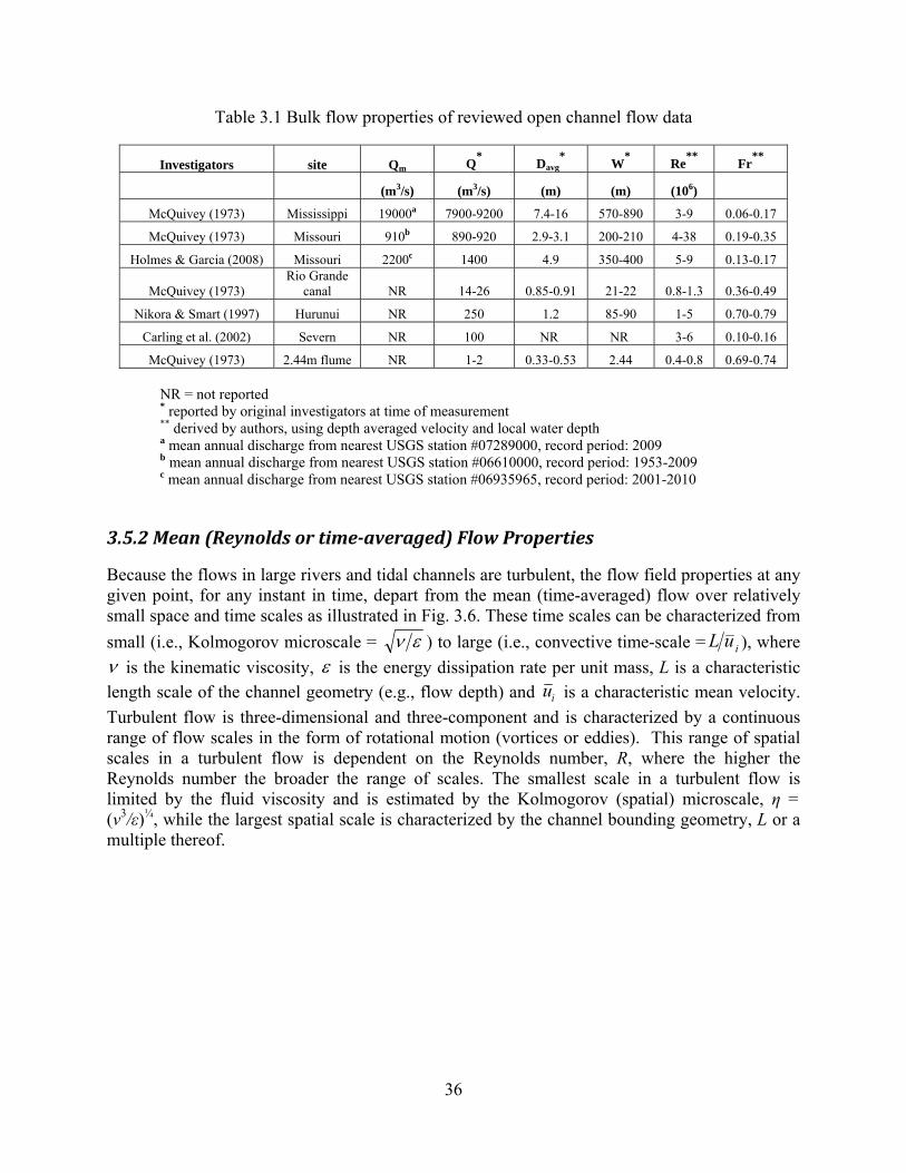
R and F are nondimensional numbers that indicate the flow state and flow regime. R above 2000-4000 indicates that inertial forces dominate over viscous forces, which causes instabilities and turbulence. Since R in natural channel flows in large rivers and tidal channels are typically well over 105, these flows are in a turbulent flow state. F below one indicates that the celerity or speed of propagation of a small surface wave ℎ is greater than the bulk velocity (i.e. gravitational forces dominate over inertia). F for large rivers and tidal channels are typically less than one, indicating subcritical flow regimes in which the flow upstream is influenced by downstream conditions. Examples of bulk flow properties for large rivers reported by Neary and Sale (2010) are summarized in Table 3.1. All Reynolds numbers are above 400,000 and Froude numbers indicate subcritical flows for all measurements with the maximum Froude number occurring for the Hurunui River in New Zealand (Nikora & Smart 1997).

36

Table 3.1 Bulk flow properties of reviewed open channel flow data

Investigators site Qm Q* Davg

* W

* Re

** Fr

**

(m3/s) (m3/s) (m) (m) (106)

McQuivey (1973) Mississippi 19000a 7900-9200 7.4-16 570-890 3-9 0.06-0.17

McQuivey (1973) Missouri 910b 890-920 2.9-3.1 200-210 4-38 0.19-0.35

Holmes & Garcia (2008) Missouri 2200c 1400 4.9 350-400 5-9 0.13-0.17

McQuivey (1973) Rio Grande

canal NR 14-26 0.85-0.91 21-22 0.8-1.3 0.36-0.49

Nikora & Smart (1997) Hurunui NR 250 1.2 85-90 1-5 0.70-0.79

Carling et al. (2002) Severn NR 100 NR NR 3-6 0.10-0.16

McQuivey (1973) 2.44m flume NR 1-2 0.33-0.53 2.44 0.4-0.8 0.69-0.74 NR = not reported * reported by original investigators at time of measurement ** derived by authors, using depth averaged velocity and local water depth a mean annual discharge from nearest USGS station #07289000, record period: 2009 b mean annual discharge from nearest USGS station #06610000, record period: 1953-2009 c mean annual discharge from nearest USGS station #06935965, record period: 2001-2010

3.5.2 Mean (Reynolds or time‐averaged) Flow Properties 

Because the flows in large rivers and tidal channels are turbulent, the flow field properties at any given point, for any instant in time, depart from the mean (time-averaged) flow over relatively small space and time scales as illustrated in Fig. 3.6. These time scales can be characterized from

small (i.e., Kolmogorov microscale = ) to large (i.e., convective time-scale = ), where

is the kinematic viscosity, is the energy dissipation rate per unit mass, L is a characteristic length scale of the channel geometry (e.g., flow depth) and is a characteristic mean velocity.

Turbulent flow is three-dimensional and three-component and is characterized by a continuous range of flow scales in the form of rotational motion (vortices or eddies). This range of spatial scales in a turbulent flow is dependent on the Reynolds number, R, where the higher the Reynolds number the broader the range of scales. The smallest scale in a turbulent flow is limited by the fluid viscosity and is estimated by the Kolmogorov (spatial) microscale, η = (ν3/ε)¼, while the largest spatial scale is characterized by the channel bounding geometry, L or a multiple thereof.

iuL

iu

37

Fig. 3.6 Definition sketch defining coordinate system and mean and instantaneous flow profiles. Turbulence occurs in both wall bounded (solid surfaces such as the bed floor) and in free shear flows such as wakes of devices, shown in Fig. 3.6. In addition to these turbulent inflow structures, unsteady downstream flow structures, that may be locally turbulent, may exist such as vortical flow structures and unsteady or cyclic flow shedding. The types of vortical flow structures that would be dependent on device design and mounting configuration, but may consist of blade tip vortices, tower / bed-floor junction vortices and Karman vortex street associated with flow shedding off of structures. The downstream wake of the device will consist of both large scale (on the order of the rotor plane) and smaller scale flow structures. The large or macro-scale momentum deficit wake of the device may have a rotational flow pattern related to blade rotation and will have characteristics cyclic frequencies associated with the blade passage frequency. The smaller scale structures will consist of individual wakes, vortices and flow unsteadiness as illustrated in Fig. 3.6 Proper characterization of both the inflow and downstream flow features is important in determining overall device performance in single and array deployments. While the mean flow resources directly impact long term device output and performance, it is the short term unsteady flow characteristics which impact unsteady loads on the device components, vibration and sound generation.

3.5.2.1 Mean (Time‐averaged) Velocity 

The instantaneous velocity component v, w is decomposed into its time-mean and

turbulent fluctuation, along its respective axis , y, z as illustrated in Fig. 3.6.

The instantaneous velocities u, v, w are defined herein as the streamwise, cross-stream, and

u

u

mean flow profile

Turbulent inflow

Blade & towerWakes

Tip vortices

Flow shedding

Blade Rate: blade passage frequency

Neary et al 2010Junction vortices

z,w

,uui 'iii uuu xxi

38

vertical velocity component, respectively. The most common means of characterizing a flow field is to measure the statistics of the flow from mean velocity up through higher order statistics such as the flow skewness and kurtosis. These statistical measures can provide a wealth of information related to the time or space averaged flow, however, they do not provide a measure of the scale and of the instantaneous, unsteady flow structures that may be important in generating unsteady loads, vibration and noise. These unsteady flow structures tend to have smaller spatial scales with higher magnitude fluctuations and local gradients than the time averaged profiles would suggest.

3.5.2.2 Turbulence Intensity and Reynolds Stresses  

The turbulence intensity is a vector quantity with each component derived from the three normal Reynolds stress terms in the Reynolds-averaged-Navier-Stokes (RANS) equation

where each instantaneous velocity component v, w is decomposed into its time-mean

and turbulent fluctuation, along its respective axis , y, z. The instantaneous

velocities u, v, w are defined herein as the streamwise, cross-stream, and vertical velocity component, respectively. The RANS equation states that the rate change of momentum of a fluid element per unit volume is balanced by the forces per unit volume acting on the fluid element. Forces on the right hand side of the equation include the gravitational body force, the mean drag force, the isotropic hydrostatic pressure force, viscous stresses, which are negligible outside the viscous sublayer, and Reynolds stresses caused by turbulence. The Reynolds stress tensor is symmetric and includes six terms, three along the diagonal that are normal stresses, and the three non-diagonal terms that are shear stresses.

The Reynolds stress tensor physically represents the momentum flux or transport of one fluctuating velocity component by the fluctuating or turbulent velocity components, However, it is a mathematical statistical quantity defined by the velocity fluctuation variance and cross-

correlations. The square root of the normal stresses divided by the density, , , , are denoted alternatively in the literature as turbulence intensities, root mean squares (RMS),

, , , or standard deviations, . It should be noted that the

''

jii

j

j

i

ijj

iij

jiuu

x

u

x

up

xfg

x

uu

,uui 'iii uuu xxi

''

''''

''''''

ww

wvvv

wuvuuu

''uu ''vv ''ww

RMSu RMSv RMSw ,ui ,v w

39

Reynolds stress tensor is not invariant under coordinate system rotation and the magnitude of the measured stresses is a function of the flow direction. Accurate measurement and interpretation of the Reynolds stresses can be problematic due to the mathematical definition of the quantities where noise, instrument motion and spatially and temporally varying flow structures can contribute significantly to the magnitude of these statistics. The following laboratory or field test phenomena can impact the accuracy of the measurement of the Reynolds stresses. Ambient or instrument noise floors can increase the auto-correlation statistics and reduce the cross-correlation estimates. These noise sources will increase the spectral noise floor masking some features of the flow spectra and can be of a flat white noise spectral nature or frequency dependent. It will be shown later that ADV noise is component dependent the off-axis components exhibiting higher noise floors than the on-axis component. This increased noise in two of the three components of velocity will not only bias the normal statistics (increasing variance) but will also decrease the cross-correlations or Reynolds shear stress measurements. The instrument spatial resolution and frequency response must be sufficient to resolve the flow features of interest. Poor spatial and temporal resolution will impart a low-pass filtering effect on the measured data. Flow induced vibration of the instrument, device or system can impact the statistical measures in both uncorrelated and/or correlated manners that can bias both the auto and cross correlation statistics respectively. Finally, flow features associated with non-turbulent oscillating or meandering flow structures, flow shedding or cycle-to-cycle flow variations in cyclic flows can show up as a pseudo-turbulence to a fixed point, non-moving measurement probe. The data acquisition and processing of the measurement signals can also impart a bias to the processed statistic or may be needed to properly assess flow structure and scale. For example, noise filtering or other de-noising techniques may inadvertently filter or bias processed data. Phase encoded sampling or multi-point measurements may be needed to accurately determine flow scale size, strength and duration. Probe vibration compensation is a complicated problem to address and will be discussed later. Historically the streamwise turbulence intensity, σu, has been adopted as a measure of the amount of turbulence. This is likely a result of the limitation of one-component instruments for measuring turbulence, like hot-wire anemometers, that were used in the past (e.g., McQuivey, 1973). A second measure is horizontal turbulence intensity, which includes both streamwise and cross-stream components. A third measure of turbulence at a point is the turbulent kinetic

energy, which includes all turbulence intensity components, TKE = 0.5 .

Turbulence intensities are commonly normalized by the shear velocity, u* or the local streamwise mean velocity, . The hear velocity is defined by √τw where τw is the skin friction at the solid boundary and is the fluid density and can be estimated by several different methods such as from the logarithmic velocity profile or the linear Reynolds shear stress distribution (see Biron et al., 2004 for a comparison of six different methods). Relative turbulence intensity is referred to as σi/u* and σi/ .

In the inner flow region of a fully developed turbulent boundary layer, turbulence is scaled by inner variables such as u* and the kinematic viscosity ν if the law of the wall is satisfied (Nezu and Nakagawa, 1993). This region is close to the wall (bed) at z/D < 0.2, where z is the vertical

)( 222

wvu

u

u

40

height above the bed and D is the flow depth. An approximate scaling of turbulence by u* is as well obtained farther away from the wall in the intermediate flow region 0.1 < z/D < 0.6 where there is a balance between turbulent energy production and dissipation. Nezu and Nakagawa (1993) derived semi-empirical equations to describe relative turbulence intensity in the intermediate flow region indicating a decrease in relative turbulence intensity with increasing distance from the bed:

These equations have been shown to give good predictions of measured relative turbulence intensity profiles over unobstructed smooth and rough bed open-channels irrespective of Reynolds and Froude numbers (Nezu and Nakagawa, 1993). Comparison by Neary and Sale (2010), which includes additional high Reynolds number river turbulence measurements, supports this observation. Measurements of mean velocity and relative turbulence intensity for rivers with large Reynolds numbers compared to laboratory flumes are rare due to the difficulty of deploying acoustic Doppler velocimeters in deep flows with fast currents. The data compiled and evaluated by Neary and Sale (2010) represents, to the authors’ knowledge, all known turbulence measurements reported to date for rivers over one meter depth, including those by Nikora and Smart (1997) and Holmes and Garcia (2009). Results are shown in Figs. 2.5 and 2.7. Flow depths in this data set vary from approximately D = 0.5 m to 35 m for the Mississippi River with mean velocities ranging from = 0.5 m/s to 3.8 m/s. Considering the challenge of accurate

measurements of turbulence in large rivers, as well as the difficulty in estimating the shear velocity, the comparison between measured and predicted profiles shown Fig. 2.7 indicates that Nezu and Nakagawa’s models 1-3 perform fairly well in large rivers.

The derivation of the above exponential equations is based on the k-ε turbulence model (Nezu and Nakagawa, 1993) where turbulent energy production and dissipation are in local equilibrium. These equations are only applicable in the intermediate region of a fully developed turbulent boundary layer. These equations (and u* scaling) should not be used for developing or disrupted boundary layers such as those induced by flow separation (McLean et al., 1994) and/or in altered flows. Scaling by u* in the wake of bluff bodies is incorrect as the flow structure is no longer influenced by the local bed geometry and turbulent energy generation is not equal to dissipation.

Normalization (or scaling) of turbulence statistics is performed to evaluate and compare values between studies under varying flow and boundary conditions (e.g., experiments with differing bed roughness) and to develop universal expressions. For these objectives, the absolute magnitude of the turbulence is less important than the normalized turbulence statistics. However, for studies investigating MHK device-flow interactions, it is important to take into consideration the magnitude of the turbulence experienced by the device. Turbulence levels in laboratory experiments may not exceed the thresholds found in natural flows, which may cause an undesirable loading that affects efficiency and fatigue. Normalizing turbulence by u* or tends to obscure the magnitude of the turbulence experienced as illustrated by comparing streamwise

DzuTKE

Dzu

Dzu

Dzu

w

v

u

/2exp78.4

/exp27.1

/exp63.1

/exp30.2

2*

*

*

*

u

u

41

intensity, nondimensionalized shear velocity (Fig. 2.7) with its dimensionalized value. Normalizing by the shear velocity masks the effect of the streamwise velocity and Reynolds number and could have a marked impact on the experimental observations and conclusions. For example, the normalized turbulence intensity measured in two separate experimental setups may be quite similar, while the turbulence magnitudes could be of different orders.

42

4. INSTRUMENTATION, DEPLOYMENT AND MEASUREMENT PROTOCOLS

4.1 BATHYMETRIC MAPPING WITH ECHOSOUNDERS

Bathymetric mapping techniques recommended for MHK site resource characterization include single and multi-beam depth echosounders (SBE, MBE) coupled to a global positioning system (GPS) that is capable of receiving differential GPS corrections. Each of these techniques is illustrated in Fig. 4.1 below. Bathymetric mapping using these techniques is preferable at the high water depths corresponding to flows above the mean annual discharge because unsubmerged portions of the channel reach cannot be mapped.

Fig. 4.1 Depth Echosounder using: (a) single beam; and (b) multi-beam. Borrowed with permission from Muste et al. (2010).

As shown in Fig. 4.1, high resolution MBE can resolve bed forms, such as sand dunes, and large roughness elements.

4.2 SEDIMENT PROPERTIES, BED FORMS, SUBSTRATE COMPOSITION,

ROUGHNESS AND SUBSTRATE STABILITY

4.2.1 Bed Forms 

High resolution SBE and MBE can be used for measuring the wavelength and height of bed forms. Substrate samples using methods described below should be obtained to determine the composition of the bed and any spatial variations in substrate composition.

43

4.2.2 Substrate Core and Grab Sampling Equipment and Methods 

Sediment samples collected in deep waters are normally collected using either a springloaded sediment dredge, benthic grab sampler (Fig. 4.2), gravity core sampler, Ogeechee core sampler, VibeCore-D sampler (Fig. 4.3) or other similar equipment. Standard operating procedures for sediment sampling are detailed in TVA-KIF-SOP-05, Revision 2 (Environmental Standards, Inc. 2010):

(a) Locate sediment sampling locations based upon the project work control documents; (b) Locate sediment sampling locations using a portable GPS unit, if possible; (c) Document locations in the field logbook and conduct photo-documentation in

accordance with the Photograph Management SOP (TVA-KIF-SOP-26); (d) Use a properly decontaminated sampler to collect sediment samples; (e) When using a spring-loaded sediment dredge or benthic grab sampler, lower the

sampler into place in an open position, and trip the sampler to close; (f) If necessary, subdivide the sample into the appropriate depth intervals when using a

core sampler; (g) Log the sediment sample according to the USCS or the Burmeister Classification

System in the field logbook or on project-specific soil boring logs. The Ponar Type Grab sampler (Fig. 4.2) is a commonly used sampler that is very versatile for bottoms consisting of sand, gravel and clay. However, this type of sampler is not suitable for bottoms consisting of moderate to large cobbles.

Fig. 4.2 Ponar-type grab samplers (Rickly Hydrological Company 2010).

44

ASTM Standard D4823 - 95(2008) covers core-sampling submerged, unconsolidated sediments. It also covers terminology, advantages and disadvantages of different types of core samplers, core-distortions that may occur during sampling, techniques for detecting and minimizing core distortions, and methods for dissecting and preserving sediment cores. Sampling procedures and equipment are divided into categories based on water depth. Critical dimensions and properties of open-barrel and piston samplers like the cutting-bit angle, core-liner diameter, inside friction factor, outside friction factor, area factor, core-barrel length, barrel surfaces, and chemical composition of sampler parts shall conform to this standard guide. The following factors shall be considered for decisions in choosing between an open-barrel sampler and a piston sampler: depth of penetration, core compaction, flow-in distortion, surface disturbance, and repenetration. Driving techniques included in this guide are free core samplers, implosive and explosive samplers, punch-corer samplers, vibratory-driven samplers and impact-driven samplers. Guides are also included for collecting short cores in shallow water, collecting long cores in shallow water, and collecting short and long cores for a range of water depth. Field record shall be provided for every sampling operation. Guides are also provided for core extrusion for samplers with no liners, slitting core and core liners, sectioning cores, sampling through liner walls, preserving cores, and displaying cores. Other standards to consult include: Tennessee Valley Authority (TVA). Field Documentation SOP (TVA-KIF-SOP-06), February 2009; TVA. Field Quality Control Sampling SOP (TVA-KIF-SOP-11), April 2009; TVA. Photograph Management for the TVA Kingston Fossil Plan Ash Recovery Project SOP (TVA-KIF-SOP-26), October 2009; TVA. Standard Operating Procedure for Sediment Sampling SOP (TVA-KIF-SOP-05, Revision 2), June 2010; TVA. Sampling Labeling, Packing, and Shipping SOP (TVA-KIF-SOP-07), 2009; Specialty Devices, Inc. VibeCore-D Operating Manual. Revision 5, March 2008. It should be recognized that collecting bottom or core samples from deep, fast moving waters is not a common activity and complications may be encountered when following standard protocols described above.

45

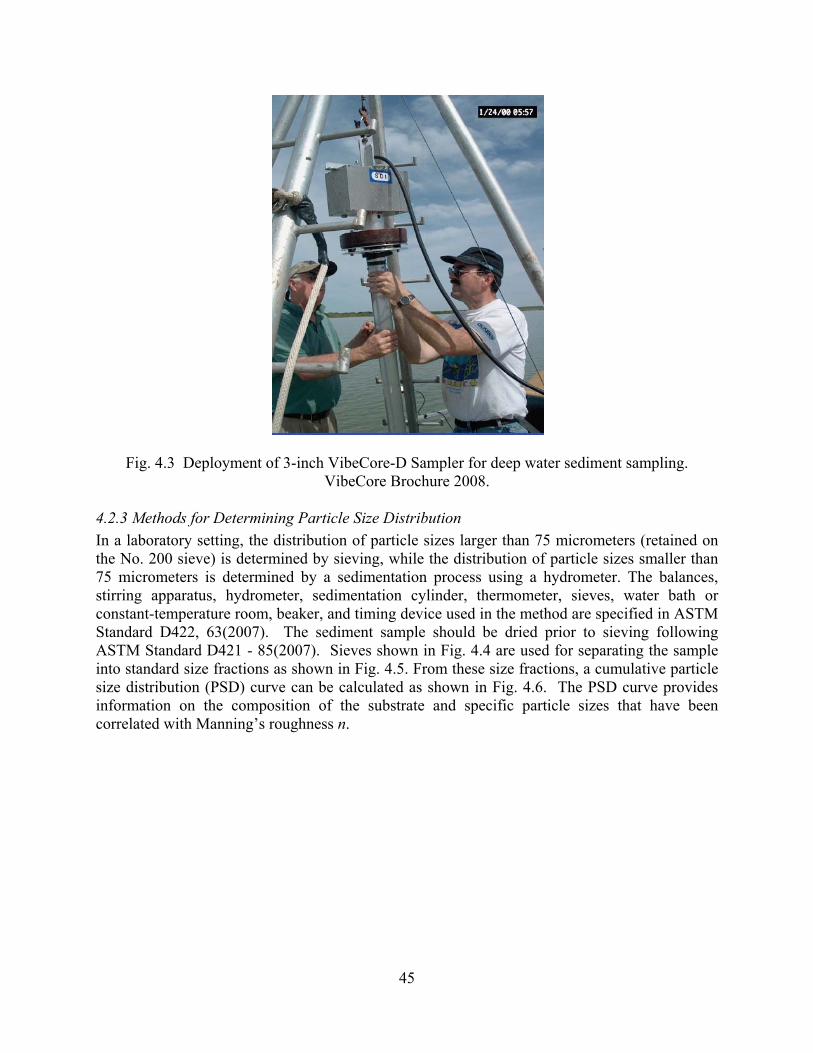
Fig. 4.3 Deployment of 3-inch VibeCore-D Sampler for deep water sediment sampling. VibeCore Brochure 2008.

4.2.3 Methods for Determining Particle Size Distribution

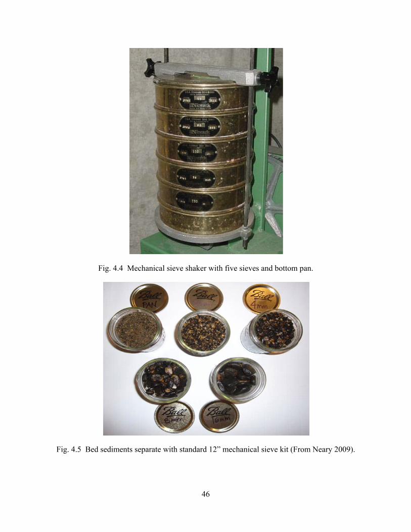
In a laboratory setting, the distribution of particle sizes larger than 75 micrometers (retained on the No. 200 sieve) is determined by sieving, while the distribution of particle sizes smaller than 75 micrometers is determined by a sedimentation process using a hydrometer. The balances, stirring apparatus, hydrometer, sedimentation cylinder, thermometer, sieves, water bath or constant-temperature room, beaker, and timing device used in the method are specified in ASTM Standard D422, 63(2007). The sediment sample should be dried prior to sieving following ASTM Standard D421 - 85(2007). Sieves shown in Fig. 4.4 are used for separating the sample into standard size fractions as shown in Fig. 4.5. From these size fractions, a cumulative particle size distribution (PSD) curve can be calculated as shown in Fig. 4.6. The PSD curve provides information on the composition of the substrate and specific particle sizes that have been correlated with Manning’s roughness n.

46

Fig. 4.4 Mechanical sieve shaker with five sieves and bottom pan.

Fig. 4.5 Bed sediments separate with standard 12” mechanical sieve kit (From Neary 2009).

47

Fig. 4.6 Cumulative particle size distribution to determine surface roughness of gravel stream channel (Neary 2009).

Other important standards to reference include ASTM D 2487 Standard Practice for Classification of Soils for Engineering Purposes (Unified Soil Classification System), and the Burmeister Soil Classification Naming System. (Burmeister 1949). Sediment data for MHK resource characterization should be reported following protocols by Poppe et al. (2003) as single-point vector datasets with sample identifiers, navigation, textural attribute information, and metadata. In-situ optical measurements are possible, either to measure turbidity (optical backscatter - OBS) or sediment size distribution (laser in-situ sizing and transmissometry - LISST). Calibration against laboratory samples may be required. Further, progressive biofouling may complicate long-term optical measurements of suspended sediment.

4.3 TEMPERATURE AND PRESSURE

Vented cabled temperature-pressure sensors are available from a number of vendors to record water temperature T [] and pressure p [FL-2]. density [ML-3] and kinematic viscosity [L2T-1]. For example, the In-Situ Troll 500 has a media-isolated piezoresistive silicon strain gauge pressure sensor with a range that can be rated up to 70 m, an accuracy of 0.1% full scale and resolution of 1 mm. The temperature sensor uses a platinum resistance thermometer with a range of -5oC to 50oC, accuracy of 0.1 C, and resolution of 0.01oC.

48

4.4 TURBIDITY AND CONDUCTIVITY

Turbidity is commonly observed with a nephelometer, which measures the fraction of source light scattered at 90o. Conductivity sensors may be divided between those which are actively pumped and those which make a passive measurement. Pumped sensors are more accurate, but the power requirements for the pump may be problematic for stand-alone deployments. For either type of conductivity sensor, biofouling is a concern for long-term deployments, as shown in Fig. 4.7. Because instrument resolution and accuracy varies with scale range, some initial assessment of turbidity and conductivity is necessary for optimal sensor selection.

Fig. 4.7 Salinity measurements obtained from northern Admiralty Inlet, WA with a Seabird 16plus v2 showing the effect of biofouling in the salinity step change during instrument turn-

around.

4.5 MEAN (REYNOLDS OR TIME-AVERAGED) FLOW PROPERTIES

4.5.1 Velocity Measurements using Acoustic Methods 

As described by Muste et al. (2010):

“ … an acoustic pulse (ping) of a known frequency (F) is sent out by a transducer into the water column along the acoustic beam. A fraction of that acoustic pulse is reflected by small particles in the water return to the transducer at a frequency (F`) that has been shifted due to the Doppler effect. The water velocity along the acoustic beam is determined using the Doppler shifts of sound waves reflected from the particles moving with the water velocity (V). The change in signal amplitude or frequency (the frequency shift is actually determined from the slope at zero shift of the covariance function) in conjunction with the travel time is used to estimate the location of the measurement and the velocities along the beam path.”

49

Fig. 4.8 Acoustic Doppler velocity instruments: a) illustration of the Doppler effect; b) ADV for

point measurements; c) Horizontal ADCP for instantaneous horizontal velocity profiles; d) ADCP for instantaneous measurement of vertical velocity profiles. From Muste et al. (2010).

50

Muste et al. (2010) describe the three most commonly used acoustic instruments used for velocity measurements in the field. Acoustic Doppler Velocimeters (ADV) measure flow velocities using the Doppler shift principle (Kraus et al. 1994). The instrument typically consists of a sound emitter, three or four sound receivers, and a signal conditioning electronic module. An ADV can measure 2D or 3D water velocity components within a small sampling volume (of the order 1 cm3) at short distance (between 5 and 18 cm) from the instrument head (see Fig. 4.8b) with sampling frequencies up to 200 Hz. However, most common implementations of ADV systems are limited to frequencies below 50 Hz due to processing algorithms, acceptable levels of measurement uncertainty and measurement stand off distances. ADVs are well suited to characterize mean flow and some turbulence characteristics at discrete points (Nikora and Goring, 2004; Nystrom et al., 2007, Gunawan et al. 2008; Fox and Belcher, 2009; Thomson et al. 2010). For large rivers or tidal flows, the greater challenge is stably deploying the ADV at the discrete point of interest. Acoustic Doppler Current Profilers (ADCP) have continuously been developed since their inception in the early ‘80s (Christensen & Herrick, 1982; Gordon 1989; Simpson, 2001). There is a vast literature describing ADCP’s underlying principles, configuration, and operational aspects (e.g., Gordon, 1989; Simpson and Oltman, 1993; RDI, 1996; Sontek, 2000). ADCPs transmit sound pulses (pings) pointing in several directions (typically 3 or 4) in the water column, and subsequently listen to the returning echoes from particles moving in the acoustic beam (Fig. 4.8d). The echo received from a pulse traveling through the water column is range-gated to produce successive segments, called depth cells or bins (see Fig. 4.8d). The relative velocity between ADCP and particles in each depth cell is determined using the frequency difference between transmitted and echoed acoustic signals due to Doppler frequency shift (narrow band system) or using the phase difference between two superimposed echoes (pulse coherent and broad band system). Coordinate transformation is then used to convert measured velocities from beam to instrument coordinates (accounting for beam angle and orientation) and then instrument to earth coordinates (accounting for pitch, roll, and heading). A three beam ADCP is a minimum requirement to provide three component current velocity in each bin whereas a four beam ADCP provides an extra velocity component useful for estimating the error resulting from inhomogeneous sampling (beam divergence throughout the water column). When the ADCP is deployed from a moving platform such as a boat, an autonomous underwater vehicles (AUV) or a remotely operated vehicle (ROV), the relatively velocity between the ADCP and the earth is required for computing the relative velocity between the particles and the earth. The movement of the ADCP relatively to the earth is typically measured using GPS or the ADCP bottom tracking capability, a feature commonly available in ADCPs. Horizontal Acoustic Doppler Current Profilers (HADCP) are an ADCP variant which utilize monostatic transducers that are fixed on special side-looking mounts (see Fig. 4.8c). Acoustic pulses are sent horizontally into the water body along two horizontal diverging beams. A signal processing software is used to analyze the returning beams to calculate multiple velocities from numerous range-gated sample volumes (bins) along the beam path. The HADCP output is a two-component horizontal water velocity profiles along a line across the channel cross section.

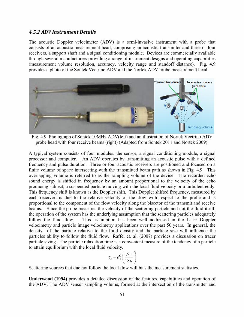
51

4.5.2 ADV Instrument Details 

The acoustic Doppler velocimeter (ADV) is a semi-invasive instrument with a probe that consists of an acoustic measurement head, comprising an acoustic transmitter and three or four receivers, a support shaft and a signal conditioning module. Devices are commercially available through several manufacturers providing a range of instrument designs and operating capabilities (measurement volume resolution, accuracy, velocity range and standoff distance). Fig. 4.9 provides a photo of the Sontek Vectrino ADV and the Nortek ADV probe measurement head.

Fig. 4.9 Photograph of Sontek 10MHz ADV(left) and an illustration of Nortek Vectrino ADV

probe head with four receive beams (right) (Adapted from Sontek 2011 and Nortek 2009). A typical system consists of four modules: the sensor, a signal conditioning module, a signal processor and computer. An ADV operates by transmitting an acoustic pulse with a defined frequency and pulse duration. Three or four acoustic receivers are positioned and focused on a finite volume of space intersecting with the transmitted beam path as shown in Fig. 4.9. This overlapping volume is referred to as the sampling volume of the device. The recorded echo sound energy is shifted in frequency by an amount proportional to the velocity of the echo producing subject, a suspended particle moving with the local fluid velocity or a turbulent eddy. This frequency shift is known as the Doppler shift. This Doppler shifted frequency, measured by each receiver, is due to the relative velocity of the flow with respect to the probe and is proportional to the component of the flow velocity along the bisector of the transmit and receive beams. Since the probe measures the velocity of the scattering particle and not the fluid itself, the operation of the system has the underlying assumption that the scattering particles adequately follow the fluid flow. This assumption has been well addressed in the Laser Doppler velocimetry and particle image velocimetry applications over the past 50 years. In general, the density of the particle relative to the fluid density and the particle size will influence the particles ability to follow the fluid flow. Raffel et. al. (2007) provides a discussion on tracer particle sizing. The particle relaxation time is a convenient measure of the tendency of a particle to attain equilibrium with the local fluid velocity.

2

18p

s pd

Scattering sources that due not follow the local flow will bias the measurement statistics. Underwood (1994) provides a detailed discussion of the features, capabilities and operation of the ADV. The ADV sensor sampling volume, formed at the intersection of the transmitter and

52

receiver beams, is typically a cylindrical volume on the order of several mm in diameter with a length that is comparable to the diameter. The sampling volume is displaced from the probe head due to the probe head design. The absolute displacement is a function of probe design and can vary from several cm to over 15 cm.

4.5.3 ADCP Instrument Details 

Acoustic Doppler Current Profilers (ADCPs) work by transmitting acoustic pulses (for example at 150-1200 kHz) from each of two to five diverging acoustic transducers (Fig. 4.10). A four transducer arrangement is known in literature as a Janus configuration. After the pulse is emitted, the ADCP then listens to and processes returned echoes from successively farther away water volumes along the beams to determine how much the frequency has changed. The difference in frequency between transmitted and reflected sound is proportional to the relative velocity between the ADCP and the scattering particles in the water based on the Doppler shift. The profiling range over which an ADCP can resolve water velocities depends upon the frequency of the acoustic signal. Generally, the lower the frequency, the farther the ADCP can measure through the water column, however greater the Doppler uncertainty, all other settings being equal. For example, a 600 kHz RDI workhorse can profile up to 40m depth, with a single ping Doppler uncertainty of ~14 cm/s (0.5m bin, 3 m/s ambiguity velocity), while a 1200 kHz unit has a single ping uncertainty of ~9 cm/s, but a range of only 15m. ADCPs have been widely used to collect water velocity profiles in oceans and streams (e.g. Schott 1987; Gordon 1989; RDI 1996; Cook et al. 2007; Gunawan 2010; Gunawan et al. 2010a; Richmond et al. 2010; Thomson et al. 2010).

Fig. 4.10 Different types of ADCP beam configurations (RDI 2011)

A four-beam ADCP measures four 1D water velocities at a depth h along the axis of each acoustic beam as shown in Fig. 4.11. Note that other configurations of transducer beams are also possible. These 1D beam velocities sample only a small volume of water because the acoustic beam emitted by each transducer is intentionally focused and narrow. Measurement from each pair of beams produces one horizontal and one vertical velocity components (Fig. 4.12). Hence, under the assumption that water currents do not change significantly in magnitude or direction (homogeneous) in the plane perpendicular to the transducers’ mutual axis, two horizontal and one vertical velocity components can be combined to compute a profile of 3D water velocity at the depth h. The surplus in the vertical velocity component can be used to calculate an error velocity, the difference between the two vertical velocity components, which indicates the homogeneity of the velocity in a horizontal layer. It should be noted that even if the homogeneity assumption is violated for resolving a 3D velocity vector, the 1D velocity profiles

53

collected along each beam are still valid measurements. The size of the 3D velocity measurement sampling volume can be expressed as the volume of a cylinder along the four beams with the bin size as its height (Fig. 4.13). The sampling volume increases with increasing distance from the ADCP. Care must be taken when the sampling volume is large as it may bias the statistics away from small scale structures. Detailed description of the coordinate transformation can be found in RDI (1998b). For further detail about the working principle of ADCP, see RDI (1996 & 1998a) and Simpson (2001).

Fig. 4.11 Beam velocity components at a depth cell (RDI 1996).

Fig. 4.12 Resultants of east-west and north-south velocities (RDI 1996).

h

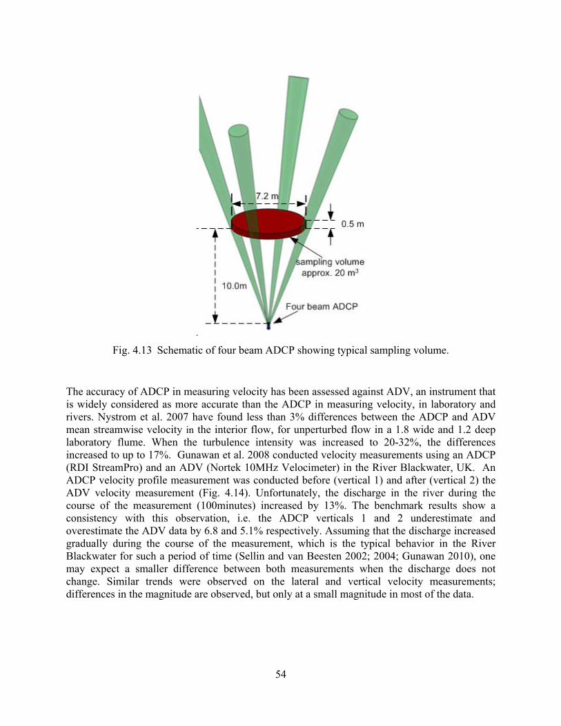
54

Fig. 4.13 Schematic of four beam ADCP showing typical sampling volume.

The accuracy of ADCP in measuring velocity has been assessed against ADV, an instrument that is widely considered as more accurate than the ADCP in measuring velocity, in laboratory and rivers. Nystrom et al. 2007 have found less than 3% differences between the ADCP and ADV mean streamwise velocity in the interior flow, for unperturbed flow in a 1.8 wide and 1.2 deep laboratory flume. When the turbulence intensity was increased to 20-32%, the differences increased to up to 17%. Gunawan et al. 2008 conducted velocity measurements using an ADCP (RDI StreamPro) and an ADV (Nortek 10MHz Velocimeter) in the River Blackwater, UK. An ADCP velocity profile measurement was conducted before (vertical 1) and after (vertical 2) the ADV velocity measurement (Fig. 4.14). Unfortunately, the discharge in the river during the course of the measurement (100minutes) increased by 13%. The benchmark results show a consistency with this observation, i.e. the ADCP verticals 1 and 2 underestimate and overestimate the ADV data by 6.8 and 5.1% respectively. Assuming that the discharge increased gradually during the course of the measurement, which is the typical behavior in the River Blackwater for such a period of time (Sellin and van Beesten 2002; 2004; Gunawan 2010), one may expect a smaller difference between both measurements when the discharge does not change. Similar trends were observed on the lateral and vertical velocity measurements; differences in the magnitude are observed, but only at a small magnitude in most of the data.

55

Fig. 4.14 Comparison of ADV and ADCP data in the middle of a meandering river cross-

section: (a) time allocation of measurements, (b) streamwise velocity, (c) lateral velocity, (d) vertical velocity (Gunawan et al. 2008).

4.5.4 ADV and ADCP Deployment Methods 

Common ADV deployments include stationary tower or tripod mounted instruments (Fig. 4.15). ADVs are sometimes cable deployed as well (Fig. 4.16). Towers provide a stable platform for long term ADV measurements on the order of weeks to months, which is necessary for flow characterization at a tidal channel site. However, towers and tripods obstruct a greater percentage of the flow section and care must be taken when considering stationary deployment so as not to create vortex shedding and flow alteration within the sample volume of the ADV. Fig. 4.16 shows an ADV probe mounted on a short cantilever displacing the probe head and sample volume upstream of the sounding weight. The cantilevered arm is kept short to minimize arm vibration but must be long enough to position the sample volume out of any weight induced flow variations. Cable deployed ADVs allow a greater number of measurement points compared to tower mounted ADVs. However, it is difficult to accurately position the sampling volume at

b)

c)

a)

d)

56

the desired locations in the water column. Furthermore, the spatial stability or stable position holding capacity of the sounding weight may be compromised in the wake of a MHK device or underwater obstruction. The sounding weight may exhibit oscillatory motion or vibration in response to the intermittent, rotating blade wakes downstream of a MHK device. This flow induced motion will be transferred to the ADV probe upstream of the weight, as shown in Fig. 4.16, resulting in increased uncertainty in the 3-component ADV measurement due to sample volume motion and varying probe alignment relative to the true flow direction.

Fig. 4.15 Stationary tripod deployed ADV and ADCP used for Marrowstone Island, WA deployment (Richmond et al. 2010).

Fig. 4.16 Cable-deployed ADV (CDADV) with sounding weight (Photograph courtesy of Bob

Holmes, USGS, 2010).

57

Common ADCP deployment methods include mooring and riverbed/seabed mounted for stationary measurements, as shown in Fig. 4.17. The stationary measurements refer to fixing the ADCP at a location to sample the data at a period of time. This method provides accurate mean velocity data when some samples are averaged over a long period, and can be used to monitor water level changes. Another type of measurement is the ADCP moving-boat measurement. For this type of measurement, the ADCP is mounted on an underwater vehicle (Fig. 4.17c), a remote-controlled boat (Fig. 4.17d) or a large ship (Fig. 4.18). Then, the ADCP measures velocity data while the boat is moving. This method is suitable to obtain velocity data for a large region of interest, such as for the tidal current resource assessment of a region or flow field characterization of river cross sections. Cable deployed ADCP is suitable for undertaking the ADCP moving-boat measurement in smaller rivers (i.e. up to 50m width). The cableways system can be a mobile (Fig. 4.19) or a fixed one (Fig. 4.20). The advantage of using a mobile cableway system lies in the way that it can be deployed or moved quickly and, potentially, be used at various flow conditions (e.g., in bank and overbank flows, as demonstrated in Gunawan et al. 2010b and Gunawan 2010).

Fig. 4.17 ADCP deployment methods: (a) mooring, (b) mounted, (c) underwater vehicle, (d) remote controlled boat (RDI 2011b; Muller and Wagner 2009).

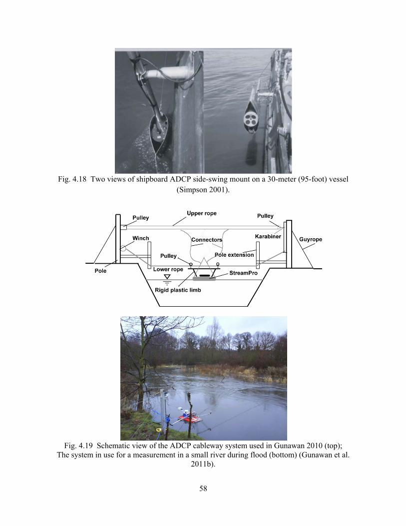
58

Fig. 4.18 Two views of shipboard ADCP side-swing mount on a 30-meter (95-foot) vessel

(Simpson 2001).

Fig. 4.19 Schematic view of the ADCP cableway system used in Gunawan 2010 (top);

The system in use for a measurement in a small river during flood (bottom) (Gunawan et al. 2011b).

59

Fig. 4.20 ADCP cableway systems for flow measurement in inbank and overbank flow

conditions at River Teme, UK (Gunawan, unpublished data).

4.5.5 ADV Error and Signal Processing Methods 

4.5.5.1 Sources of Error 

Many investigators have attempted to address sources or error and the impact of noise on turbulence measurements (Voulgaris and Trowbridge 1998; Nikora and Goring 1998; Finelli et al. 1999; Hurther and Lemmin 2001; Garcia et al. 2005; Garcia et al. 2007). Spatial resolution filtering, signal acquisition / sampling frequency, signal processing and system noise can impact measurement accuracy. Sample rate and signal processing can incur a low-pass temporal filtering as well as a velocity alias error. System noise, which typically includes sampling errors (channel drop outs or loss of coincidence), Doppler noise, gradient errors and multi-probe signal contamination can also bias mean and turbulence velocity estimates. Some of these noise sources can be scaled or frequency dependent. Apart from these systematic errors, human error such as inaccuracy in aligning the ADV probe can alter the data significantly. ADVs operate utilizing acoustic Doppler shift, so unexpected reflections of the transmitted signals have the potential to severely compromise the integrity of collected data. Unexpected reflections may occur if an acoustic pulse that has encountered a boundary is received during the same interval as data reflected from the particles within the sampling volume, namely the volume defined by the intersection of the receiver “beams” (often conceptually simplified to be a

Fixed cableway system

Mobile cableway system

60

cylinder). The effects of boundary interference are most pronounced and only of significant concern when the boundary enters into the sampling volume. Finelli et al. (1999) explored the effects of sample volume proximity to the boundary layer on measurements acquired by ADV instruments. Having empirically measured the size of the sampling volume, they found it to be substantially larger than the nominal value provided by the manufacturer. In their literature, they include their method for measuring the sample volume and caution users to the importance of appropriately positioning the device in order to extract meaningful data. Prior to deployment and data collection, the ADV user must specify the range of velocities that is expected to be sampled in the flow. Aliasing or over-ranging is a problem that arises from particles in the sampling volume moving toward the transducers at a rate beyond that prescribed by the user. Phase shift can only be measured in the range 0o – 360o. Hence, the measurement will start again from 0o once phase passes 360 o. In such a case, an abrupt change in the velocity (a spike) is likely to occur with a change in sign. For a system with only one dominant flow direction, such as in open channel, the aforementioned condition may bias the mean longitudinal velocity towards lower value. While some ADVs allow for velocity ranges approaching a magnitude of five meters per second which would encompass any smaller ranges and practically eliminate the problem of over-ranging, the greater the velocity range setting results in an increased production of noise by the instrument. The effects of noise can also seriously affect the accuracy of data, and so the selection of the velocity range should be carefully considered. It is important for the user to assess the anticipated range of unsteady velocities that may be encountered in any flow component. Often spurious data do not manifest as spikes but as underlying noise. This is especially relevant in the case of ADV technology since the devices themselves produce a Doppler noise which appears in the data as white noise, thereby affecting high statistical moments and obscuring trends in the power spectra. The magnitude of Doppler noise is affected by instrument model, fluid characteristics and flow conditions that include flow velocity, presence and type of particles in the flow, and turbulence (Nikora and Goring 1998, Cea et al. 2007). Nikora and Goring (1998) attempted to quantify the Doppler noise by measuring velocity of still water with different seeding particles and ADV velocity range settings. The result shows that the magnitude of the Doppler noise for different spectra bands is more or less the same. They then used the result to correct velocity measurements with the same ADV velocity range setting. Fig. 4.21 shows the typical auto-spectra plot for longitudinal velocity component and the white noise level measured in an outdoor flume. Nikora and Goring (1998) show that Doppler noise in still water appears as white noise. However, correcting the auto-spectra of moving water velocity with the white noise obtained from still water measurement is not appropriate when the magnitude of the Doppler noise is changing with increased water velocity. Note that the velocity spectra begin to flatten at higher frequencies at the same order of magnitude with the average Doppler noise. Voulgaris and Trowbridge (1998) introduced the term ‘noise floor’ to describe the flat power spectra density, which also correspond to the total noise of the instrument. The noise floor may not be apparent unless sampling at sufficiently high sampling rates. An ADV measurement is an average over a sample volume with spatially nonuniform velocities rather than the velocity at a single point. As a result errors associated with spatial averaging are present. Again, the user should be cognizant of the flow scales of interest when selecting a

61

measurement device. A large measurement volume will spatially low-pass filter the velocity field and may bias the statistics away from small scale structures that may be important for unsteady loading and system vibration and noise. The frequency at which ADVs make measurements is greater than the frequency of the data provided to the user. And so, the data provided to the user represents an average of the measured data. The averaging process is a digital nonrecursive filter (Hamming 1983; Bendat and Piersol 2000). This filtering affects the power spectrum by removing energy bands beyond the cut-off frequency and reduces the even moments of the signal (García et al. 2005). In general, the frequency limit in the measured data will be at least ½ the sampling frequency due to the Nyquist criteria and may be even lower due to processing contraints.

Fig. 4.21 Typical auto-spectra for longitudinal velocity component and white noise level

calculated from measured Doppler Noise (Nikora and Goring 1998)

4.5.5.2 Protocols for Reducing Error 

The majority of common errors may be avoided with the application of a few simple protocols outlined below. Determining the vertical size of the sample volume The identification of the boundaries of the sampling volume is important so that the validity of the data is not being compromised by boundary interference that may occur when the ADV is in close proximity to solid boundaries, e.g. moorings, cables, etc. Specifications on the dimensions and placement of the sample volume provided by manufacturers are imperfect. Therefore, in order to enhance the reliability of data sampled by these devices, therefore, it is important to determine the actual size of the sampling volume with greater certainty. Finelli et al. (1999) describes the method which they implemented for measuring the dimensions of the sampling volumes of their devices. They created an acoustic target using two lengths of monofilament fishing line stretched across the interior of a trash can filled with tap water such that the lines intersected at near right angles in the center of the tank. The water was allowed to sit for a substantial length of time so that any suspended gases could be released and any sediment could settle. The probe was positioned directly over the target at a sufficient distance so that the sampling volume did not encompass the target, i.e. the SNR was uninfluenced by the target, and

62

data were sampled for ten seconds. The instrument was then lowered slightly and another set of data were sampled. This process was continued until the sampling volume had passed the target entirely. Calculating the average SNR for every sample, the researchers were able to identify the bounds at which the target began to influence the data and so identify the bounds of the sampling volume. Dimensionless Frequency Criteria García et al. (2005) defined a dimensionless frequency and prescribed the conditions to ensure that the effects of aliasing are not biasing collected data. They presented present the following inequality:

20

where F, fR , L, and Uc are the dimensionless frequency, sampling frequency, energy containing length scale, and convective velocity respectively. If the above inequality is observed then the effects of aliasing as well as temporal averaging should be negligible. In measurements downstream of rotating devices, it is important to understand the characteristic flow features and their frequency content to avoid low-pass filtering of these flow features. Histogram Inspection Effects of over-ranging on data are easy to identify. The probability density function (PDF) of a time series (in the beam coordinate system) may demonstrate a sudden velocity cut-off beyond which no data will be registered. If this abrupt discontinuity is observed in a data sample, the user should increase the user defined velocity range until the histogram of the time series no longer demonstrate such characteristics. Optimally the user should select the smallest velocity range (in either beam or earth coordinates) for which no cut-off is observed in the histogram.

4.5.5.3 Methods for Error Removal 

In cases where spurious data cannot be avoided, the data can be reconstructed so that the assumptions drawn from the data are representative of the characteristics of the flow. Correlation threshold Correlation is a measure of the similarity of two pulse echoes being measured by the Doppler instrument. Zero correlation means the two echoes are unrelated, where as a correlation of 1 means the two echoes are identical. High correlation is desired because it indicates confidence that the system measured the two pulses it originally sent out and is determining a valid phase shift. In practice correlations of zero are not observed because of noise due to electronics, temperature fluctuations, and other factors will always cause correlation. Correlation reported by the instrument will be on a percent scale from 0-100%, so simply multiplying the above limits by 100 will place them in the appropriate range. In the early days of the acoustic Doppler velocimeter, if a user did some tests and determined correlations were above ~70% then the instrument was considered to be generating good quality data. Many users still use this number for screening out bad data, although a generalization to some universal value is unwarranted and

63

a close examination of the dataset is the best way to set a correlation threshold (if any) for discarding bad data points. Spike Identification, Removal and Replacement Petrie et al. (1988) and Baldwin et al. (1993) first applied a velocity hodograph elliptical filtering technique to laser Doppler velocimeter measurements as an effective means of filtering LDV measured noise. In this technique, the measured data are rotated into the principal stress coordinates and an elliptic filter of size N principal stresses in the minor and major axes is applied to the 2-D probability density function (PDF). Velocity ensembles occurring outside the defined ellipse are filtered from the data set. Fontaine et al. (1996) extended the 2-D elliptic filter technique to the 3-D flow application with a principal stress 3-D ellipsoid filter on three-component LDV measured data. The Phase-Space Thresholding (PST) PST technique developed by Goring and Nikora (2002) is another ellipsoidal filter technique where invalid points are identified as those lying outside of the universal threshold defined ellipsoid in a three dimensional Poincaré phase space. While the ellipsoidal filter technique of Fontaine et al operates on the instantaneous velocity hodograph (u vs v vs w) with filtering applied in the principal stress space, the PST technique operates on the instantaneous velocity and it’s local accelerations (u vs du/dt). The PST technique has been critically analyzed and improved upon by a number of peers (Wahl 2003, Pasheh et al. 2010). The use of the PST algorithm has grown in acceptance and is now the standard means of filtering data (Gunawan et al. 2011a). Nevertheless, improvements to the PST algorithm have been proposed to address the main criticism that it was replacing valid data around spikes. While removal has negligible effects on the value of bulk statistical moments, it has been shown by (Pasheh et al. 2010) to compromise time dependent indicators such as the power and energy spectra. Goring and Nikora have suggested cubic interpolation by the twelve points on either side of an identified invalid datum and seem to be one of the few researchers to have compared various methods. Pasheh et al. (2010) have proposed a modified Phase-Space-Thresholding Sample and Hold algorithm (mPST-SH) that evaluates the validity of data in three stages: first any velocity measurements near the average are incontrovertibly marked as valid, then any data far from the average are marked as invalid and are removed, finally the data are filtered using the PST technique. Data Processing in Beam Coordinates Data are originally measured in beam coordinates, however, ADV software allows the user to select which coordinate system he/she would like for data output, including beam, Cartesian (XYZ) or Earth (East North Up (ENU)) coordinates. As previously discussed, over-ranging occurs when particles in the sampling volume move toward one of the transducers at a rate beyond that prescribed by the user. When analyzing the measured Doppler phase shift, such data cannot always be resolved and the associated velocity is erroneously translated into the assigned velocity range resulting in a spike in the data. It is recommended that all acoustic measurements should be recorded and processed in beam coordinates because the spike will only occur in one of the beam coordinate time series. If coordinate transformation is employed before such a spike is removed, the spike may be obfuscated by the linear transformation and also may affect the other components, rendering identification of the spike more difficult. As such it is suggested that users always record their data in the beam coordinate system and only after appropriate error

64

removal procedures have been implemented, should they convert to another coordinate system Doroudian et al. (2007). Spectral Noise Filter A spectral analysis technique by Voulgaris and Trowbridge (1998) was suggested by Goring and Nikora for removing the effects of noise within the noise floor of the power spectra at higher frequencies by the average of the noise spectrum. “The empirical spectra of the Doppler noise are replaced by straight horizontal lines whose ordinates are equal to the average of the noise spectral ordinates.” (Goring and Nikora 1998, García et al. 2005). The power spectra can then be reverse Fourier transformed to generate a noise filtered time series. For some applications, it is also possible to remove the bias from Doppler noise in the time domain (e.g., Thomson et al. 2010 for turbulence intensity).

4.5.6 ADCP Data Quality Control and Post‐processing 

The following sections detail typical procedures used ADCP data acquisition, synchronization, and post processing for quality control of data. Quality control procedures vary from one ADCP experiment to another, depending on the experimental setup and quality of data.

4.5.6.1 Preventing Interference between Acoustic Instruments 

When two or more active acoustic instruments are deployed in close proximity or on the same mooring, there is potential for mutual interference (cross talk). This can occur for two instruments operating at the same frequency or at integer multiples of a common frequency (e.g., a 50 kHz depth sounder will cause interference for a 300 kHz ADCP). Additionally, side bands adjacent to the primary instrument frequency may contain enough acoustic energy to cause mutual interference. This interference may be obvious in a review of measurements (e.g., non-physical values with a strong periodicity as shown in Fig. 4.22) or may be more subtle. In one case with shipboard ADCP measurements contaminated by a depth sounder (Polagye, unpublished data), data were post-processed by rejecting bins with velocities five standard deviations greater than the average for a transect. By definition this requires discarding some fraction of the measurements and eliminating the source of the cross-talk is preferred. If two or more instruments are deployed together, the simplest option to prevent mutual interference is to adopt a duty cycle under which no two instruments are simultaneously transmitting or listening. While this is straightforward to realize for an instrumentation package with a central controller, clock drift may lead to complications for stand-alone instruments. For example, if internal clocks drift in opposite directions, mutual interference may occur periodically over the duration of the deployment. Failure to account for cross-talk may meaningfully distort statistics on a temporal or spatial basis.

65

Fig. 4.22 Shipboard ADCP measurements of currents (m/s) contaminated by cross-talk (top) and

post-processed with most interference removed (bottom).

4.5.6.2 Correcting for Clock Drift 

Internal clocks for different pieces of instrumentation may drift over the course of a deployment. This complicates the process of data assimilation, as two measurements with the same time stamp may not be sampling the same event. While the use of a centralized controller with a single clock simplifies assimilation, it also introduces a single point of failure into an instrumentation package, which may be undesirable. Assuming that clock drift is linear over the deployment, time stamps may be corrected through the following procedure:

Configure and deploy instrument from a computer with a clock recently synchronized with an NTP source.

Upon instrument recovery, compare instrument clock with NTP source. Compute difference between instrument and NTP and correct instrument time stamps,

assuming a linear drift. If the clock drift is relatively minor in comparison to the phenomena of interest, it may be possible to neglect it without effect.

4.5.6.3 Measurements near Boundaries 

Acoustically solid boundaries (hard substrate, water surface) contaminate adjacent bins as side lobe reflection from the solid boundary obscures returns from sound scatterers for the primary beam. The zone of expected contamination is given by:

66

, where H is the water depth and φ is the beam angle relative to vertical (e.g., 20o). In practice, this zone may be somewhat larger or smaller and can be visually identified in a time series out by spuriously high velocities or spurious directional shifts, as shown in Fig. 4.23. For a 20º beam angle ADCP deployed upward looking, the echoes from the side lobe sound reflected by the water surface are received by the transducers at the same time as the echoes from the main lobe sound reflected by the particles in the water at 94% of the ADCP distance to the surface (RDI 1996). The ADCP data are contaminated from this distance onwards to the water surface. Whereas, RDI 1996 reported that 94% of the ADCP distance to the surface is the threshold for side lobe interference, other researchers have experienced threshold values less than that (e.g., Gunawan et al. 2010). Another common source of bias relative to measurement volume size and proximity to a surface is the impact of the spatial scale of the flow gradient relative to the measurement volume size. It is a common practice to bury a part of the sampling volume in the bed floor or surface with the intent on obtaining a velocity measure as close to the surface as possible. While this practice can increase noise, it can also bias the velocity statistics through the alteration of the velocity ensemble PDF. The PDF may be incorrectly weighted towards higher velocities if large gradients are present with a scale that is small relative to the sampling volume, or the PDF may show a bi-modal distribution with a zero-velocity mode due to ensembles of the wall or bed-floor velocity.

Fig. 4.23 Contamination of horizontal current velocity within 4m of the free surface for a

bottom-mounted ADCP (Polagye, unpublished data)

cos1 HD

67

4.5.6.4 Velocity Quality Control 

Spikes in velocity measurements within a burst need to be removed. One of the approaches to remove spikes is to use a threshold value. For this approach, the differences between the velocities from consecutive measurements in a burst for all the corresponding bins are calculated. If these differences are higher than the specified threshold value, they are removed. This quality control step removes the spikes in the velocity measurements for every burst. This procedure is repeated for all the bursts acquired from ADCP measurements. It should be noted that the threshold values for quality control depend on test conditions, experimental setup and quality of data. Another approach is to use the Phase-Space Thresholding (PST) or the modified Phase-Space Thresholding (PST) algorithms to detect the spikes and then to replace the outliers (Goring and Nikora 2002; Pasheh et al. 2010). Both algorithms are available in the codes, developed by ORNL, to post process the ADV and ADCP data (Gunawan and Neary 2011a; Gunawan et al 2011a).

4.5.6.5 Lack of Scatterers issue 

Velocity data cannot be measured when sound scatterers do not exist in the water column. The amount of suspended sediments in rivers is generally sufficient to produce strong echoes. In an ocean environment, lack of scatterers at a certain depth is not uncommon. For example, on a cruise near Mauritius only one-third of the nominal range contain velocity data, and this kind of condition is occurring less than 10% of the time (RDI 1996).

4.5.6.6 Transducers Ringing 

The ADCP cannot measure velocity in a small region adjacent to the transducers due to transducer ringing. ADCP transducers vibrate for a while after transmitting sound pulses and, during this time, the returned echoes are contaminated by the vibration (ringing). The time required until the ringing dissipates, often referred to as the blanking period, corresponds to the distance of the first bin from the transducers that can be measured by the ADCP. The typical blanking distance for a 300kHz and a 1200kHz RDI ADCP is 2m and 0.5m, respectively (RDI 1996).

4.5.6.7 Velocity Ambiguity 

Phase shift can only be measured in the range of 0o – 360o. Hence, the measurement will start again from 0o once the phase passes 360o. In this case, an abrupt change in the velocity (a spike) is likely to occur (Figure 2-6). A change of sign occurs when the phase shift exceeds 360o but is still below 720o. No change of sign occurs when the phase shift exceeds 720o but is still below 1080o. In order to overcome this issue, prior to deployment and data collection, the ADCP user must specify the maximum velocity expected to be sampled in the flow (the ambiguity velocity). The ambiguity velocity is the maximum allowable radial motion for phase measurements to be unambiguous.

4.5.6.8 Moving‐bed Condition 

ADCP bottom track or GPS data is required to take into account the movement of the ADCP when calculating water velocity. The ADCP bottom track fails if high amounts of material, such

68

as clay or sand, are moving near the bed. Such a condition typically happens during high flow; whereas, high velocity causes the bed to be eroded. A moving bed condition can be detected by examining the ADCP stationary measurement data. The presence of the moving bed condition is indicated by significant movements of the ADCP shown in the data during a stationary measurement.

4.5.6.9 Air bubbles 

Breaking waves generate bubbles below the ocean surface. Passing under the ship’s hull, the bubbles can act as a shield that distracts the transmission of sound pulses. They can reduce the ADCP profiling range and, in the worst case, completely block the sound transmission.

4.5.6.10 Temporal averaging 

One method often used to reduce the velocity fluctuations in the ADCP data is to average the data over a reasonably long period of time (e.g., 3 to 15 minutes). This method has become a standard in post-processing the ADCP stationary measurement in rivers. After averaging for a certain period of time, the mean velocity becomes statistically stable, i.e., it does not change significantly with more samples to be averaged. The averaging time to obtain stable mean streamwise velocity in rivers depends on many variables, such as the flow characteristics of the site and bin size; but is typically less than 15 minutes. A summary of the suggested averaging time by different researchers is presented in Table 4.1. Gunawan (2010) reported that out of 31 stationary measurements undertaken at two river cross sections, 30 satisfied the 5% convergence level for the mean streamwise velocity when averaged over 300s. The 5% convergence level indicates that the difference between the mean streamwise velocity averaged over 300s and the last 20 samples is less than 5%. Knowledge of the minimum averaging time is beneficial, especially when conducting a stationary measurement using a boat-mounted ADCP (the boat position is fixed during the measurement). Using the minimum averaging time ensures that adequate accuracy on the mean velocity profile is achieved within the shortest measurement time possible. Table 4.1 Minimum averaging time for ADCP stationary measurement in rivers suggested by different researchers.

Source Barua & Rahman Stone & Hotchkiss Szupiany et al Gunawan

(1998) (2007) (2007) (2010) Suggested averaging time 900s 100 - 250s 420 - 600s 300s

River width ~ 11,000m 12.8 -15.4m 600 – 2,500m ~ 5 - 8m

River depth 8.3 - 10m 0.75 – 1.1m 5 – 12m ~0.6 – 1.2m

ADCP model RDI Broadband ADCP

1200kHz RDI Broadband Rio Grande ADCP

1000kHz SonTek ADP

2MHz RDI Broadband StreamPro ADCP

Sampling frequency 0.5Hz ~1Hz 12Hz 1Hz

Bin size 50cm 5cm 50 - 75cm 5-10cm

Max. boat movement 3m N/A 5m 0.1m

69

4.5.6.11 Spatial averaging 

ADCP moving-boat measurement method can be used to obtain the flow field in a river cross-section (see also Gunawan and Neary 2011a, section 2.4 for more details). However, the data obtained using such a method contains some random errors (Muste et al. 2004). Averaging several ADCP transects together reduces the data fluctuation due to random errors and turbulence (Dinehart and Burau 2005; Szupiany et al. 2007; Gunawan et al. 2010a). An example of a transect averaging result is shown in Fig. 3.5. One of the key points when conducting transect averaging is to ensure that the transect data are obtained at the same cross section. Dinehart and Burau (2005) averaged the velocity data from each ADCP transect by interpolating them into a 2D grid representing the cross section of the corresponding measurement. The value at each node of the grid was calculated using an inverse distance weighting (IDW) method (six samples points were selected by an equipartite arrangement). Each set of the interpolation grids was averaged together to obtain the final velocity grid. Szupiany et al. (2007) used a SonTek ADP (Acoustic Doppler Profiler) to measure the 3D velocity in River Parana, Argentina, at several cross sections of 600-2400m widths. Szupiany et al. (2007) suggests that the finer detail of the existence of secondary flow cells can be obtained by averaging five transects. Le Coz et al. (2007) used the IDW method to average the ADCP transect data obtained from a 100m wide river. Their results suggest that the number of data points considered for calculating the IDW interpolation value at each node of the grid affects the smoothness of the velocity profiles in the IDW-interpolated grid. As a quality measure, Le Coz et al. (2007) report that the difference between the discharge in the river before and after the IDW interpolation is always within 3%. Gunawan et al. (2010a) reported that the transect averaging results depend on the size of the interpolation grid and the distance between the measurement data point and the IDW interpolation node in the grid. When a data point is too close to the interpolation node, the velocity value at that data point has a dominant influence on the interpolated velocity at the node. If the data point close to the interpolation node is a spike, the IDW interpolation method will only have a minor effect in smoothing the spike. Gunawan (2010) conducted measurements in two river cross sections and compared the depth-averaged streamwise velocity of the ADCP transect averaging results and the time-averaged stationary ADCP data; a typical example of the data is shown in Fig. 4.24. An average difference of 3.4% was reported (Fig. 4.25). A research is currently being conducted to further assess the accuracy of the ADCP moving-boat measurement data (Gunawan and Neary 2011b; Gunawan et al. 2011c).

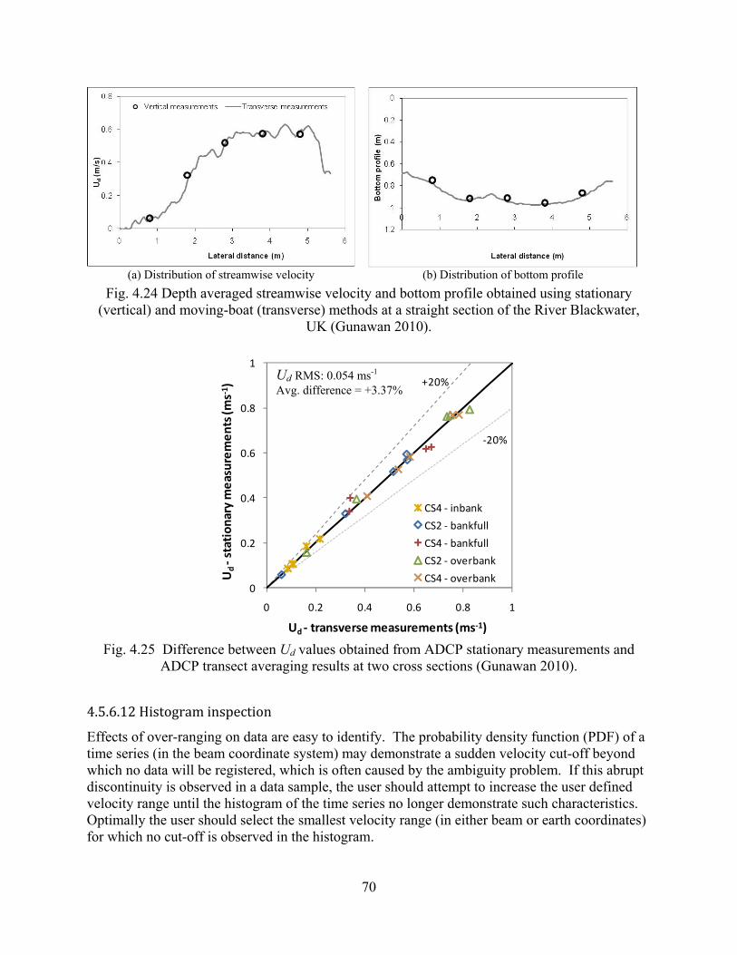
70

(a) Distribution of streamwise velocity (b) Distribution of bottom profile

Fig. 4.24 Depth averaged streamwise velocity and bottom profile obtained using stationary (vertical) and moving-boat (transverse) methods at a straight section of the River Blackwater,

UK (Gunawan 2010).

Fig. 4.25 Difference between Ud values obtained from ADCP stationary measurements and

ADCP transect averaging results at two cross sections (Gunawan 2010).

4.5.6.12 Histogram inspection 

Effects of over-ranging on data are easy to identify. The probability density function (PDF) of a time series (in the beam coordinate system) may demonstrate a sudden velocity cut-off beyond which no data will be registered, which is often caused by the ambiguity problem. If this abrupt discontinuity is observed in a data sample, the user should attempt to increase the user defined velocity range until the histogram of the time series no longer demonstrate such characteristics. Optimally the user should select the smallest velocity range (in either beam or earth coordinates) for which no cut-off is observed in the histogram.

+20%

‐20%

0

0.2

0.4

0.6

0.8

1

0 0.2 0.4 0.6 0.8 1

Ud‐stationary measurements (m

s‐1 )

Ud ‐ transverse measurements (ms‐1)

CS4 ‐ inbank

CS2 ‐ bankfull

CS4 ‐ bankfull

CS2 ‐ overbank

CS4 ‐ overbank

Ud RMS: 0.054 ms-1

Avg. difference = +3.37%

71

4.6 ADV AND ADCP MEASUREMENTS AT MARROWSTONE ISLAND, WA

Hydrokinetic site characterization presents an instrumentation trade-off for some metrics of interest, particularly turbulence. An ADV is able to sample at much higher frequency and lower noise than an ADCP, thereby more accurately characterizing the velocity spectra. However, measurements are limited to a small volume O(1 cm3) and positioning an ADV at the elevation of interest (e.g., turbine hub height) may be infeasible in strong currents. Conversely, an ADCP profiles the entire water column, resolving variations across the energy extraction plane, and may be readily deployed from a surface mooring or anchored on the seabed. This measurement does, however, have a greater potential for error from spatial averaging of multiple beams and greater noise than for an ADV. A study was conducted in 2010 off Marrowstone Island, Puget Sound, WA to evaluate the relative merits of ADVs and ADCPs for hydrokinetic site characterization. This site has previously been identified as having currents in excess of 2 m/s, but is in water shallow enough for diver operations (Gooch et al. 2009). This preliminary field study was carried out by the Pacific Northwest National Lab (PNNL) in collaboration with the Applied Physics Lab at the University of Washington (APL-UW) (Thomson et al. 2010, Richmond et al. 2010). This study entailed ADV and ADCP measurements from 4th May 2010 to 22nd May 2010. A Nortek Vector (6 MHz) ADV and an RDI Workhorse Sentinel (600 kHz) was used by Thomson et al. (2010) to measure all three components of velocity at the Marrowstone Island (MI) site. The ADV provided high temporal resolution data at a single point 4.6 m above the seabed and was setup to acquire 64 s of data every 10 minutes. A 10% duty cycle helped conserve power and memory for two weeks of deployment at the site. At every burst, the ADV recorded data for 64 s at a sampling frequency of 32 Hz, thereby collecting 2048 data points for every single burst. This sampling scheme was used to capture high-frequency fluctuations of velocity within a burst, with each burst being assumed to be quasi-stationary. The ADCP collected low temporal resolution velocity profile data from the seabed up to the surface and was setup to acquire data every 30 minutes in order to conserve power and memory for two weeks of deployment. The ADCP recorded data for 64 s at a sampling frequency of 2 Hz, thereby collecting 128 data points for every single burst in each bin. The data were recorded in beam coordinates in order to avoid the assumption of homogeneity required in the East-North-Up (ENU) coordinate system transformation. The ADCP recorded data from 2.6 m above the seabed up to the surface at a vertical bin resolution of 0.5 m.

4.6.1 Mean Velocities and Power Densities 

The first step in analyzing the data acquired from the ADV measurements described above was to calculate the mean velocity data from each individual ADV burst. Fig. 4.26 shows the mean velocities for the Marrowstone Island site. As shown in the figure, u and v components of velocity (horizontal velocity components) show a tidal variation, i.e., changing direction and magnitude with change in the tidal cycle. It is also observed that the w component of velocity (vertical velocity) is significantly less than the horizontal velocity components. The next step was to calculate the horizontal velocity magnitude for each burst; these values are shown in Fig. 4.27. As seen in the figure, the horizontal velocity magnitude also shows tidal fluctuations. Tidal flow conditions for MHK devices can be further classified into non-slack and slack periods. A non-slack period, in general, is defined as the period of time during which the MHK

72

devices are capable of extracting energy from the flow, and a slack period is defined as the period of time during which the MHK devices are unable to extract energy from the flow. For the Marrowstone Island site, the non-slack period was assumed to occur when the horizontal velocity magnitude is greater than 0.8 m/s, and the slack period when the horizontal velocity magnitude is less than 0.8 m/s. In Fig. 4.27, the non-slack conditions are shown with red marker points. The maximum sustained velocity is defined as the highest velocity sustained over a five minute time interval or more. This is an important parameter for preliminary site evaluation and MHK design. Higher instantaneous velocities can occur anywhere in a data set, but they are not sustained for a significant period of time, therefore they are of less importance. The ADV measurements for this study were performed in bursts of 64 s, and each consecutive burst was 10 minutes apart. In this case, the maximum sustained velocity could not be determined from the method defined above. Therefore, for this study, the maximum sustained velocity was alternatively defined as the maximum velocity of the mean ADV burst. As per this alternative definition, the maximum sustained velocity at ADV deployment depth was approximately 1.4 m/s. The ADCP measurements provided the velocity profile from the seabed upward to near the water surface for the Marrowstone Island site. The horizontal velocity magnitude along with the flow direction calculated from ADCP measurements are shown in Fig. 4.28. The solid black line in the figure represents the water depth at the time of the measurements as determined from pressure data. As seen from the figure, the horizontal velocity profile, direction and depth show variations with tidal fluctuations.

Fig. 4.26 Mean velocities from ADV measurements at Marrowstone Island site.

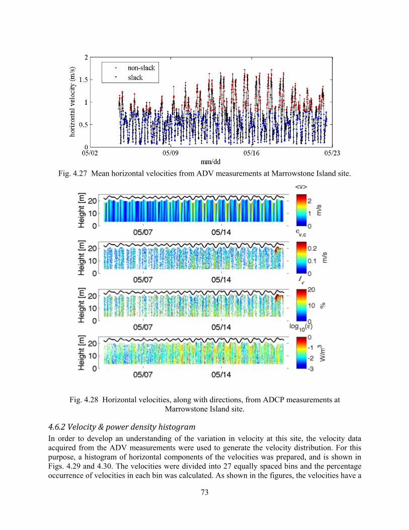
73

Fig. 4.27 Mean horizontal velocities from ADV measurements at Marrowstone Island site.

Fig. 4.28 Horizontal velocities, along with directions, from ADCP measurements at

Marrowstone Island site.

4.6.2 Velocity & power density histogram 

In order to develop an understanding of the variation in velocity at this site, the velocity data acquired from the ADV measurements were used to generate the velocity distribution. For this purpose, a histogram of horizontal components of the velocities was prepared, and is shown in Figs. 4.29 and 4.30. The velocities were divided into 27 equally spaced bins and the percentage occurrence of velocities in each bin was calculated. As shown in the figures, the velocities have a

74

bi-modal distribution, showing a diurnal tidal cycle at the site. Furthermore, a similar histogram for the horizontal velocity magnitude Vh was calculated, and is shown in Fig. 4.31. As shown in this figure, the horizontal velocity magnitude has maximum percentage occurrence of 0.8-0.9 m/s, suggesting viability of this site for installation of MKH devices. The power density P (kW/m3) was also calculated from the ADV measurements, using the equation

1

2 ℎ

where is the density of the sea water (nominal 1025 kg/m3), and v is velocity. The histogram of the power density is shown in Fig. 4.32. As shown in this figure, there is a high occurrence of available power between (0.1-0.5 KW/m2) at this site. Note that this power density is at the location of the ADV sampling point about 4.6 m above the seabed. This location would be near the bottom of the rotor sweep for most currently deployed MHK devices.

Fig. 4.29 Histogram of u-component of velocity from ADV measurements at Marrowstone Island

site.

Fig. 4.30 Histogram of v-component of velocity from ADV measurements at Marrowstone Island

site.

Fig. 4.31 Histogram of horizontal component of velocity from ADV measurements at Marrowstone

Island site.

Fig. 4.32 Histogram of power density calculated from ADV measurements at Marrowstone Island

site.

75

4.6.3 Turbulence Intensities 

The calculated standard deviations and turbulence intensities of horizontal velocities are shown in Table 1. The turbulence intensity is given by the equation

where σu and are the standard deviation and mean of the measured quantity respectively. The table shows the mean and maximum values of standard deviations and turbulence intensities from ADCP and ADV measurements. The standard deviations of the horizontal velocity calculated from ADCP measurements were significantly higher than the standard deviations calculated from ADV measurements. This is due to significantly higher noise in the ADCP measurements as compared to ADV measurements. Therefore the correction in the standard deviation values was calculated using equation

where σv,c is the corrected standard deviation, σ is the calculated standard deviation and n is the Doppler noise. After performing the correction, the standard deviations from ADCP and ADV showed similar values. Using these corrected standard deviation values, the corrected turbulence intensities were calculated for both the ADCP and ADV measurements. The corrected mean turbulence intensity of horizontal velocity was around 10%. Thus, after performing the corrections, both ADV and ADCP measurements showed similar standard deviations and turbulence intensities.

Table 4.2 ADV and ADCP statistics summary table.

ADV ADCP Measured Corrected Measured Corrected Averages values

σv (m/s) 0.09 0.08 0.22 0.11 I (%) 8% 7% 21% 10% Maximum values

σv (m/s) 0.22 0.21 0.31 0.24 I (%) 15% 14% 30% 18%

4.6.4 TKE Dissipation and Power Spectra 

The dissipation rates during slack and strong mean flow conditions are ε ~10-6 W/m3 and ε ~10-1

W/m3 respectively. The maximum dissipation rate observed for the whole deployment is 3x10-1 W/m3. These values are well within the oceanographic range; see Thomson et al. (2010) for more

,u

TI u

u

,22, ncv

76

detail. The dissipation rate is sensitive to Doppler noise and hence, agreement between the dissipation rates derived from the ADV and ADCP measurements is not observed; see Thomson et al. (2010) for further detail. To understand in detail about the flow characteristics, the power spectrum/ auto-spectral densities were calculated from ADV measurements for each velocity component. For each ADV burst, the velocities were assumed to be quasi-stationary. Therefore, for each individual burst, auto-spectral densities could be determined. Figs. 4.33 and 4.34 show typical power spectra, for all three components of velocity, for non-slack and slack conditions respectively. As observed from the figures, the power spectra are noisy, which is due to the presence of high-frequency noise in the ADV measurements. Furthermore, an ensemble average of the power spectra was calculated for the non-slack and slack flow conditions. Figs. 4.35 and 4.36 show the averaged power spectra for all three components of velocity for non-slack and slack conditions respectively. These figures show typical turbulence behavior, and for the inertial sub-range, all the three spectra have a slope of -5/3. It is also observed in these power spectrum plots that at higher frequencies, the spectra tend to become horizontal. This is due to the presence of noise in the ADV measurements. Moreover, the horizontal components of velocity show a higher noise level as compared to the vertical component (w) of velocity. The difference in noise levels of components is because of ADV beam geometry. The 30 degree tilt means that a greater projection of w is measured than u,v so both the true velocity and noise are multiplied in the projection to the horizontal plane. This difference in noise levels for different components of velocity is characteristic of ADV measurements. In addition to increased noise in the off-axis components, the shallow measurement angle (30 degrees) will translate into a higher measurement uncertainty in these two components relative to the on-axis component.

77

Fig. 4.33 Typical spectra for all components of velocity, from ADV measurements, for

non-slack period at Marrowstone Island site.

Fig. 4.34 Typical spectra for all components of velocity, from ADV measurements, for slack period at Marrowstone Island site.

Fig. 4.35 Average spectra for all components of velocity, from ADV

measurements, for non-slack period at Marrowstone Island site.

Fig. 4.36 Average spectra, for all components, from ADV measurements, for

slack period at Marrowstone Island site.

 

4.6.5 Flow Directionality 

The flow direction of the tidally driven flow is an important metric, because some MHK devices designed for bi-directional tides may not have sufficient yaw ability for asymmetrical tide conditions (Gooch et al. 2009). This asymmetry in the tidal direction may lead to significant power loss in such MHK devices. The horizontal velocity components from ADCP measurements at three different heights were extracted: (1) 4.6 m (i.e. at base of MHK devices),

78

(2) 10.0 m (i.e., at hub of MHK devices), and (3) 15.0 m (i.e. at top of MHK devices). The scatter plot of the horizontal velocity vectors for these three different heights is shown in Fig. 4.37 (a)-(c). As observed from these figures, there is a slight asymmetry in the flow direction as height from the seabed increases, which may be due to a topographical feature of the Marrowstone Island site. In these figures, the green and blue markers represent the horizontal velocity for the slack and the non-slack periods respectively. It is important to distinguish these two periods since they are an important metric for operation of MHK devices. For detailed information on directional metrics, see Gooch et al. (2009).

Fig. 4.37 Scatter plot of the horizontal components of velocity from ADCP measurements: (a) at

base, (b) at hub, and (c) at top of an MHK device.

4.7 WAVES

There are various instruments capable of carrying out wave measurements, such as Nortek AWAC, SonWave, and Teledyne RDI’s workhorse waves array. All these systems perform velocity measurements like the ADCP, and they also simultaneously acquire pressure data and/or perform acoustic surface tracking (AST), which is used to accurately determine wave height. The wave height is used along with the measured velocity to determine the amplitude, period and directional spectra of the waves. However, all the instruments mentioned above have different implementation/analysis approaches. For detailed information about the wave measurements, processing, and analysis approach for instruments from different companies, see references [8-10].

79

5. CONCLUSIONS River and tidal resource characterization for MHK technologies will require new strategies and protocols for deploying state-of-the-art acoustic instruments and processing and evaluating their data. Accurate mean flow and turbulence characteristics at the EEP will allow refined estimates of AEP and COE that cannot be obtained from coarse resource assessments. These measurements will also provide designers with important information needed to determine static and dynamic loadings that can cause fatigue and failure. The development of field protocols that can be adopted as standards in the MHK industry is therefore an important undertaking. These protocols will be refined as field experience is gained at river and tidal energy sites. This document should therefore be viewed as a starting point to identify the parameters to be measured, instrumentation and deployment strategies for their measurements, and protocols for acquiring and processing data. Important additions anticipated for future editions of this report include refined deployment strategies for acoustic instruments, the addition of detailed signal processing protocols and MATLAB codes for ADV and ADCP measurements. Depth and flow variability present challenges for characterizing river resources. The United States Geological Survey (USGS) provides flow and stage time series, but the gages may not be in close proximity to sites where resource characterization is desired, the period of record may be too short to be statistically meaningful, and river resource characterization requires accurate velocity time series to calculate energy production, structural loads, and cost of energy. Many hydrologists now believe that regional land use changes in river basins and climate change make statistical forecasting based on historical extrapolation questionable (Clarke 2007, Lima and Lall 2010). More field measurements in rivers using state-of-the-art acoustic instruments, such as acoustic Doppler current profilers (ADCP) and acoustic Doppler velocimeters (ADV), are needed to expand the limited data presently available for big rivers. Measurements of all six Reynolds stresses for rivers with utility-scale hydrokinetic potential obtained by an ADV have yet to be reported and should be undertaken. Also, the river discharge during the period of measurement should be measured and compared to the mean annual discharge and other statistical measures for low flow and flood conditions at the closest USGS gage site. Field measurements should be taken during flows that are above, close to, and below the mean annual discharge to characterize the wide range of flow conditions at a river site. Further research is needed to determine the turbulence parameters, and the ranges of scales and frequencies that are most relevant to the MHK device. This includes investigation of coherent TKE, as well as evaluation the full TKE budget, Understanding the full TKE budget may improve understanding of the residual currents unexplained by harmonic analyses and may improve predictions of turbulent feedback mechanisms during turbine operation. Research is needed on field techniques for resolving vortex shedding mechanisms and coherent eddy structures with frequencies and scales corresponding to rotational speeds and EEP dimensions. Further research is needed to improve the accuracy of acoustic measurements at river and tidal energy sites that require measurements at great depths and or high currents. To date, the authors

80

are not aware of any published studies investigating the effects of flow induced motions (FIM) or vortex induced vibrations (VIV) on ADV mean and turbulent velocity measurement accuracy, methods for reducing movement caused by FIM and VIV, and methods for tracking movement and vibrations with high-frequency accelerometers. Probe motion can impact the accuracy of the ADV and possibly bias the velocity and turbulence measurement due to 1) A relative velocity super-position between the vibrating probe head and the flow, and 2) increased uncertainty in identifying the spatial location of the vibrating sample volume. As discussed earlier, probe vibration can affect both the mean velocity measurement, depending on the vibration frequency, phase and amplitude relative to the sampling frequency and flow field characteristics (spatial and temporal scales), as well as the turbulent statistics. The magnitude of increased measurement uncertainty and any bias induced by sample volume vibration will be dependent on the frequency and amplitude of the vibration relative to the probe operating characteristics, such as pulse rate and sampling frequency It is recommended that instrument deployments include on-board instrumentation focused on quantifying the vibration and movement of velocity measuring instrumentation. Vibration measurement instrumentation may include 1) accelerometers mounted to the ADV or ADCP probes, optical, sonar or acoustic sensors mounted and operated in a differential mode designed to determine relative motion of a sensor, or 3) more sophisticated motion sensors such as GPS or IMU (inertial measurement unit) mounted to the device. If the degree of motion can be determined or quantified, data processing techniques such as frequency domain filtering or wavelet analyses may be able to be applied to the recorded signal to de-noise or correct for any velocity superposition. Unfortunately, these noise filtering techniques can filter real signal and bias the filtered result. Since the vibration induced velocity noise presents itself as a two-input

Fig. 5.1 Two input single output system (Fontaine and Neary 2011).

single output system shown in Fig. 5.1, each source independently produces a velocity component where the measured velocity is the sum of the two sources and their respective transfer functions: ˆ ˆ ˆ ˆ ˆ

m V IV H V H I .

The measured force, mV , is the sum of the flow velocity, V , times the transfer function of the

measurement instrument (calibration), VH , plus the motion of the sensor measured by, I , times

a transfer function correlating the sensor motion to a measured velocity, ˆIH . The instrument

HV

HI

Velocity field

Instrument Motion

Measured Velocity

81

transfer function is related to the instrument calibration and processing routines. The instrument vibration transfer function is determined by careful calibration of the instrument where controlled sensor vibration is induced with known frequency, direction and amplitude and the sensor output with the motion sensor output are recorded simultaneously. The true velocity field can then be deconvolved from the measured signal. While this technique would be the most accurate method of correcting for sensor vibration, it does involve detailed calibrations, additional measurements to quantify sensor motion and the vibration transfer function may be probe dependent. The accuracy of this deconvolution technique is dependent on the accuracy of the calibration and sensor motion measurements. In most applications, great care is employed to minimize probe vibration through mounting design and the use of vortex shedding damping devices. While this can be successfully accomplished in laboratory applications, it can be difficult to achieve in large scale field implementation where the probe may be mounted to large support towers that can themselves vibrate when exposed to flow or when mounted to a tethered cable anchored with a sounding weight. Fontaine and Neary (2011) recommend that these concerns be addressed in order to develop guidance for ADV deployments and measurements related to site flow characterization at rivers and tidal channels where current speeds typically exceed 1 m/s. Add-on devices for suppression of vortex-induced vibration of cylinders developed by the oil and gas industry for offshore drilling platforms might be explored for reducing VIV.

82

REFERENCES

Ashmore, P., Bergeron, N., Biron, P., Buffin-Bélanger, T., Church, M., Rennie, C.a nd Roy,

A.M. (2010) Earth Surface Processes Wiley, New York, NY. ASTM Standard D422, 63 (2007). Standard Test Method for Particle-Size Analysis of Soils.

ASTM International, West Conshohocken, PA, 2007, DOI: 10.1520/D0422-63R07, www.astm.org.

ASTM Standard D421 – 85 (2007). Standard Practice for Dry Preparation of Soil Samples for

Particle-Size Analysis and Determination of Soil Constants. ASTM International, West Conshohocken, PA, 2007, DOI: 10.1520/D0421-85R07, www.astm.org.

ASTM Standard D4823 – 95 (2008). Standard Guide for Core Sampling Submerged,

Unconsolidated Sediments. ASTM International, West Conshohocken, PA, 2007, DOI: 10.1520/D4823-95R08, www.astm.org.

American Standards for Testing and Materials (ASTM). ASTM D 2487 Standard Practice for

Classification of Soils for Engineering Purposes (Unified Soil Classification System). Baldwin,J. T., Deutsch, S., Petrie, H. L. and Tarbell, J. M., 1993. Determination of Principal

Reynolds Stresses in Pulsatile flows after Elliptical Filtering of Discrete Velocity Measurements. J. Biomech. Eng., v 115, I4a, pg 396-404.

Barua, D.K. and Rahman, K.H. (1998). Some aspects of turbulent flow structure in large alluvial

rivers. Journal of Hydraulic Research, IAHR, 36,235–252. Bathurst, James C. (2007). Effect of Coarse Surface Layer on Bed-Load Transport. ASCE

Journal of Hydraulic Engineering 133(11): 1192-1205. Bendat, J., and Piersol, A. (2000). Random data. 3rd Ed., Wiley, New York. Best J. (2005). The fluid dynamics of river dunes: A review and some future research directions.

Journal of Geophysical Research 110, F04S02, doi:10.1029/2004JF000218, pp. 21. Best, J., S. Simmons, D. Parsons, K. Oberg, J. Czuba, and C. Malzone (2010). A new

methodology for the quantitative visualization of coherent flow structures in alluvial channels using multibeam echo-sounding (MBES), Geophys. Res. Lett., 37, L06405, doi:10.1029/2009GL041852.

Bhowmik, N.G., Demissie, M. and Guo, G.Y. (1982). Waves generated by river traffic and wind

on the Illinois and Mississippi Rivers. Urbana, IL, U. of Illinois Water Resources Center Research Report 167.

83

Biron, P.M., Robson, C., Lapointe, M.F. and Gaskin, S.J. (2004). Comparing different methods

of bed shear stress estimates in simple and complex flow fields. Earth Surface Processes Landforms 29(11): 1403-1415.

Burmister (1949) Soil Classification Naming System. Modified from Principles and Techniques

of Soil Identification, Proceedings of Highway Research Board, pp. 402-433, 1949. Carling, P. A., Cao, Z., Holland, M. J., Ervine, D. A. and Babaeyan-Koopaei, K. (2002).

Turbulent flow across a natural compound channel, Water Resour. Res.,38(12), 1270. Chang (1998). Fluvial Processes in River Engineering. Krieger Publishing Company, Malibar,

Florida. Christensen, J.L. and Herrick, L.E. (1982) Mississippi River test Vol. 1, U.S. Geological Survey,

El Cajon, CA. Clarke, R.T. (2007). Hydrological prediction in a non-stationary world. Hydrol. Earth Syst. Sci.,

11(1), 408-414. Cook, C.B., Richmond, M.C. and Serkowski, J.A. (2007). Observations of velocity conditions

near a hydroelectric turbine draft tube exit using ADCP measurements. Flow Measurement and Instrumentation 18:148-155. doi:10.1016/j.flowmeasinst.2007.04.002.

Crowder, D.W., Diplas, P. (2000). Using two-dimensional hydrodynamic models at scales of

ecological importance. Journal of Hydrology, Volume 230, Issues 3-4, 8 Pages 172-191. Defne, Z., Haas, K.A., Fritz, H.M., Jiang, L., Shi, X., French, S.P., Smith, B.T., Neary, V.S.,

Stewart, K.M. (2011) National geodatabase of tidal stream power resources in the USA. Renewable and Sustainable Energy Reviews. In-Review.

Dinehart, R.L. & Burau, J.R. (2005a). Averaged indicators of secondary flow in repeated

acoustic Doppler current profiler crossings of bends. Water Resources Research, Vol. 41. Doroudian, B., Hurther, D. and Lemmin, U. (2007). Discussion of turbulence measurements with

acoustic Doppler velocimeters by Carlos M. García, Mariano I. Cantero, Yarko Niño, and Marcelo H. García, J. Hydr. Engrg. 133, 1286.

Finelli, C.M., Hart, D.D. and Fonseca, D. M. (1999). Evaluating the spatial resolution of an

acoustic Doppler velocimeter and the consequences for measuring near – bed flows, Limnology and Oceanography, Vol 44, #7, pp. 1793-1801, 1999.

Fontaine A and Neary VS. (2011). Experiments for evaluating errors in ADV measurements due

to vortex induced vibrations (VIV). ORNL/TML-2011/252, September. Fontaine, A.A., Ellis, J.T., Healy, T.M., Hopmeyer, J. and Yoganathan, A.P. (1996).

84

Identification of peak stresses in cardiac prostheses: A comparison of two-dimensional versus three-dimensional principal stress analyses, American Society Artificial Internal Organs Journal, Vol. 42, pp. 154-163.

Fox, J.F. and Belcher, B.J. (2009). Comparison of LSPIV, ADV, and PIV data that is

decomposed to measure structure of turbulence over a gravel-bed.33rd IAHR Congress, Vancouver, BC, Canada.

Garcia, C.M., Cantero, M.I., Nino, Y. and Garcia, M.H. (2005). Turbulence measurements with

acoustic Doppler velocimeters, J. Hydr. Engrg. 131, 1062 (2005). Gooch, S., Thomson, J., Polagye, B. and Meggitt, D. (2009). Site characterization for tidal

power. OCEANS 2009, MTS/IEEE. Gordon, R.L. (1989). Acoustic measurement of river dscharge. Journal of Hydraulic

Engineering-ASCE 115(7):925-936. Goring, D. G. and Nikora, V. I. (2002). Despiking acoustic Doppler velocimeter data. J. Hydraul.

Eng., 128(1) 117 - 126. Goring, D. G. and Nikora, V. I. (2003). Closure to depiking acoustic Doppler velocimeter data

by Derek G. Goring and Vladimir I. Nikora. J. Hydraul. Eng., 129(6), 487 - 488. Gunawan, B., Sun, X., Sterling, M., Knight, D. W., Shiono, K., Chandler, J., Rameshwaran, P.,

Wright, N. G., Sellin, R. H. J., Tang, X. and Fujita, I. (2008). An integrated and novel approach to estimating the conveyance capacity of the River Blackwater. Proceedings of the Eight International Conference on Hydro-Science and Engineering, Nagoya, Japan, September 8–12.

Gunawan, B. (2010). A study of flow structures in a two-stage channel using field data, physical

model and numerical modelling, PhD thesis, University of Birmingham, UK. Gunawan, B., Sterling, M. and Knight, D. W. (2010a). Using an acoustic Doppler current

profiler in a small river. Water and Environment Journal, 24: 147–158. doi: 10.1111/j.1747-6593.2009.00170.x

Gunawan, B., Sterling, M., Tang, X. and Knight, D. W. (2010b). Measuring and modeling flow

structures in a small river. Proceeding of the International Conference on Fluvial Hydraulics, Braunschweig, Germany, September 8-10.

Gunawan, B. and Neary, V.S. (2011a). ORNL ADCP Post-processing guide and MATLAB

algorithms for MHK site flow and turbulence analysis. ORNL/TML-2011/404, September. Gunawan, B. and Neary, V.S. (2011b). Accuracy of velocity data measured using ADCP moving

boat measurements. In preparation.

85

Gunawan, B., Neary, V.S., McNutt, J. (2011a). ORNL ADV post-processing guide and MATLAB algorithms for MHK site flow and turbulence analysis. ORNL/TML-2011/338, September.

Gunawan, B., Sun, X., Sterling, M., Shiono, K., Tsubaki, R., Rameshwaran, P., Knight, D.W.,

Chandler, J., Tang, X. and Fujita, I. (2011b). The application of LS-PIV to a small irregular river for inbank and overbank flows. Flow Measurement and Instrumentation. In-second review, July.

Gunawan, B., Neary, V.S., Hill, C. and Chamorro, L.P. (2011c) Accuracy of spatial and temporal

averaging of acoustic Doppler current profiler (ADCP) moving boat measurements. Poster presented at the AGU fall meeting, San Francisco, CA, December 5-9.

Guy, H. P., Simons, D. B. and Richardson, E. V. (1966) Summary of alluvial channel data from

flume experiments 1956-61: U.S. Geol. Survey Prof. Paper, 462-I,96 p. Guy (1970). Fluvial Sediment Concepts, Chapter 3 in Applications of Hydraulics, Book 3 in

Techniques of Water Resources Investigations by the US Geological Survey, US Government Printing Office, 55 pp.

Hamming, R. (1983). Digital filters, 2nd Ed., Prentice Hall, Englewood CLiffs, New Jersey Holmes, R.R. and Garcia, M.H. (2008). Flow over bedforms in a large sand-bed river: A field

investigation. Journal of Hydraulic Research, 46(3): p. 322-333. Hurther, D. and Lemmin, U. (2011). A correction method for turbulence measurements with a

3D acoustic Doppler velocity profiler. J. Atmosph & Oceanic Tech. vol 18, pp. 446-458, 2001.

Lacey, R.W.J., Roy, A.G. (2008). The spatial characterization of turbulence around large

roughness elements in a gravel-bed river. Geomorphology 102: 542-553. Le Coz, J., Gilles, P., Magali, J., and Andre, P. (2007). Mean vertical velocity profiles from

ADCP river discharge measurement datasets, Proceedings 32nd Congress of International Association of Hydraulic Engineering and Research (CD-ROM).

Le Coz, J., Pierrefeu, G. and Paquier, A. (2008) Evaluation of river discharges monitored by a

fixed side-looking Doppler profiler. Water Resources Research, 44, doi: 10.1029/2008WR006967.

Lima, C.H.R. and Lall, U. (2010). Spatial scaling in a changing climate: A hierarchical bayesian

model for non-stationary multi-site annual maximum and monthly streamflow. Journal of Hydrology, 383, 307–318.

McQuivey, R.S. (1973). Summary of turbulence data from rivers, conveyance channels, and

laboratory flumes. USGS Report 802-B Turbulence in Water.

86

Miller, K.S. and Rochwarger, M.M., (1972). A covariance approach to spectral moment

estimation. IEEE Trasactions on Infromation Theory, IT-18(5), pp. 588-596. Muste, M., Kim, D. and Merwade, V. (2010). Chapter in Gravel Bed Rivers 7: “Modern Digital

Instruments and Techniques for Hydrodynamic and Morphologic Characterization of Streams,” in Developments in Earth Surface Processes, Ashmore P., Bergeron N., Biron P., Buffin-Bélanger T., Church M., Rennie C. Roy A.M.; Wiley, New York, NY.

Muste, M., Yu, K. and Spasojevic, M. (2004). Practical aspects of ADCP data use for

quantification of mean river flow characteristics; Part I: Moving-vessel measurements. Flow Measurement and Instrumentation, 15(1), 1-16.

Neary, V.S. (2009). Physical habitat requirements of bivalvia: unionidea. Report to The Nature

Conservancy, 54 p. Neary, V.S., Constantinescu, S. G., Bennett, S. J., Diplas, P, G. Kirkil. (2010). Effects of

vegetation on turbulence, sediment transport and stream morphology. ASCE Journal of Hydraulic Engineering. Resubmitted May 1, 2010.

Neary, V.S. and Sale, D.C. (2010). Flow characteristics of river resources for hydrokinetic

energy conversion. Conference Proceedings, HydroVision International, July 27-30, Charlotte, NC.

Nezu, I. and Nakagawa, H. (1993). Turbulence in open-channel flows, A.A. Balkema,

Rotterdam. Nikora, V.I. and Smart, G.M. (1997). Turbulence characteristics of New Zealand gravel-bed

rivers. Journal of Hydraulic Engineering. 123(9): p. 764-773. Nikora, V. I. and Goring, D. G. (1998). ADV measurements of turbulence: Can we improve their

Interpretation? J. Hydraulic Eng., p. 630-634, 1998. Nortek. (2009). Vectrino velocimeter user guide. Retrieved 9/19/2011, from

http://www.nortekusa.com/en/support/manuals. Parsheh, M., Sotiropoulos, F. and Port´e-Agel, F. (2010). Estimation of Power Spectra of

acoustic-Doppler velocimetry data contaminated with intermittent spikes. J. Hydraulic Eng. ASCE, Vol.136, 368 (2010); doi:10.1061/(ASCE)HY.1943-7900.0000202.

Petrie, H. L., Samimy, M. and Addy, A. L. (1988). Laser Doppler velocity bias in seperated

turbulent flows. Exp. in Fluids, v 6, pg 80-88. Poppe, L.J., Paskevich, V.F., Williams, S.J., Hastings, M.E., Kelley, J.T., Belknap, D.F., Ward,

L.G., FitzGerald, D.M. and Larsen, P.F. (2004). Surficial sediment data from the Gulf of Maine, Georges Bank, and Vicinity: A GIS Compilation U.S. Geological Survey Open-File

87

Report 03-001. Polagye, B., Epler, J. and Thomson, J. (2010). Limits to the predictability of tidal current energy.

MTS/IEEE Oceans 2010, Seattle, WA September 20-23. Polagye, B. and J. Thomson. Noise removal from Doppler profiler measurements of turbulence.

In preparation. Raffel, M., Willert, C.E., Wereley, S.T. and Kompenhans, J. (2007). Particle Image Velocimetry

– A Practical Guide, 2nd ed., Springer. Rantz, S.E. and others (1982). Measurement and computation of streamflow: Volume 1.

Computation of discharge. U.S. Geological Survey Water Supply Paper 2175, 284 p. RDI. (1996). Acoustic Doppler current profilers - Principle of operation, A Practical Primer. San

Diego, CA, RD Instruments. RDI. (1998a). Workhouse technical manual. Teledyne RD Instruments, Inc., San Diego,

California. RDI. (1998b). ADCP coordinate transformation: Formulas and Calculations. Teledyne RD

Instruments, Inc., San Diego, California. RDI. (2011). Teledyne RDI ADCP Products. Retrieved 9/19/2011, from

http://www.rdinstruments.com/mm_products.aspx. RDI (2011). Wave primer: Wave measurements and RDI ADCP wave array technique, retrieved

9/19/2011, from: http://www.rdinstruments.com/pdfs/waves_primer.pdf Richmond, M., Thomson, J., Polagye, B. and Durgesh V. (2010). Inflow Characterization for

Marine and Hydrokinetic Energy Devices. 2010. FY2010 Annual Progress Report, PNNL Annual Progress Report to DOE EERE for FY2010

Richmond, M., Durgesh, V., Thomson, J. and Polagye B. (2011). Inflow characterization for

marine and hydrokinetic energy devices. 2011. FY2011 Annual Progress Report, PNNL Annual Progress Report to DOE EERE for FY2011.

Rosgen, D.L. (2006). Watershed assessment of river stability and sediment supply (WARSSS).

Wildland Hydrology, Ft. Collins, CO [variously pages]. Schott F. (1987). Medium-range vertical acoustic Doppler current profiling from submerged

buoys. Deep Sea Research Part A - Oceanographic Research 33(10):1279-1292. Sellin, R.H.J. and van Beesten, D.P. (2004). Conveyance of a managed vegetated two-stage

river channel. Proc. Institution of Civil Engineers, Journal of Water Management, Vol. 157, WM1, 21-44.

88

Sellin, R.H.J. and van Beesten, D.P. (2002). Berm vegetation and its effect on flow resistance in

a two-stage river channel: an analysis of field data. Proc. The International Conference on Fluvial Hydraulics, Belgium, pp.319 - 326.

Simons, D. B. and Richardson, E. V. (1966). Resistance to flow in alluvial channels. US Geol.

Surv. Prof. Pap. 422-J. 61 pp. Simpson, M.R. and Oltmann, R.N. (1993). Discharge-measurement system using an acoustic

Doppler current profiler with applications to large rivers and estuaries. Water-Supply Paper 2395, U.S. Geological Survey, Denver, CO.

Simpson, M.R. (2001). Discharge Measurements Using a Broad-Band Acoustic Doppler Current

Profiler United States Geological Survey, Sacramento, open-file report 01-1. Retrieved 9/19/2011, from: http://pubs.usgs.gov/of/2001/ofr0101/text.pdf.

Sontek (2011). 10-MHz ADV expanded description. Retrieved 9/19/2011, from:

http://www.sontek.com/pdf/expdes/10MHz-ADV-Expanded-Description.pdf SonTek (2000). Doppler velocity log for ROV/AUV applications. SonTek Newsletter, 6(1),

SonTek, San Diego, CA. SonTek/YSI (2004). Shallow water discharge measurements: SonTek flow tracer versus the RDI

StreamPro ADCP. Sontek/YSI Product Comparison, SonTek, San Diego, CA. SonWave-PRO (2008) Directional wave data collection. Retrieved 9/19/2011, from:

http://www.sontek.com/adp-adcp.php Specialty Devices, Inc. VibeCore-D Operating Manual. Revision 5, March.

Stacey, M.T., Monismith, S.G. and Burau, J.R. (1999). Observations of turbulence in partially

stratified estuary. Journal of Physical Oceanography, 29, pp. 1950-1970.42. Stone, M.C. and Hotchkiss, R.H. (2007). Evaluating velocity measurement techniques in shallow

streams. Journal of Hydraulic Research, IAHR, Vol. 45, No. 6, pp. 752 – 762. Szupiany, R.N., Amsler, M.L., Best, J.L. and Parsons, D.R. (2007). Comparison of fixed- and

moving- vessel flow measurements with an aDp in a large river. Journal of Hydraulic Engineering, 133(12), pp1299-1309.

Tennessee Valley Authority (TVA) (2009). Field documentation SOP (TVA-KIF-SOP-06),

February. Thomson, J., Richmond, M., Polagye, B. and Durgesh. V. (2010). Quantifying turbulence for

tidal power applications. 2010. OCEANS 2010, MTS/IEEE Tritico, H.M. and Hotchkiss, R.H. (2005). Unobstructed and obstructed turbulent flow in gravel

bed rivers. Journal of Hydraulic Engineering 131: 635-645.

89

TVA (2009). Field quality control sampling SOP (TVA-KIF-SOP-11), April. TVA (2009). Photograph management for the TVA Kingston fossil plan ash recovery project

SOP (TVA-KIF-SOP-26), October. TVA (2010). Standard operating procedure for sediment sampling SOP (TVA-KIF-SOP-05,

Revision 2), June. TVA (2010). Sampling labeling, packing, and shipping SOP (TVA-KIF-SOP-07), 2009. Underwood, G.N. (1994). Evaluation of a new laboratory acoustic Doppler velocimeter, MS

Thesis, Dept. of Ocean Engineering, Naval Post Graduate School, Monterey CA. USGS (2003). U.S. Geological Survey Open-File Report 03-001. Surficial sediment data from

the Gulf of Maine, Georges Bank, and vicinity: A GIS Compilation. etrieved 9/19/2011, from: http://pubs.usgs.gov/of/2003/of03-001/index.htm.

Voulgaris, G. and Trowbridge, J.H. (1998). Evaluation of the acoustic Doppler velocimeter for

turbulence measurements, J. Atmosph & Oceanic Tech., vol 15, pp. 273-289, 1998. Wahl, T. L. (2000). Analyzing ADV Data Using WinADV. 2000 Joint conference on water

resources engineering and water resources planning & management. American Society of Civil Engineers, July 30 - August 2, 2000, Minneapolis, Minnesota

Wahl, T. L. (2003). Discussion of despiking acoustic Doppler velocimeter data. J. Hydraul. Eng.,

129(6), 484 - 487.