field testing of abrasive delivery systems in winter maintenance

FIELD TESTING OF ABRASIVE DELIVERY SYSTEMS IN WINTER MAINTENANCE

By

Wilfrid A. Nixon

Funded by the Iowa Highway Research Board Project TR 458

FINAL REPORT

IIHR Technical Report # 471

IIHR—Hydroscience & Engineering College of Engineering The University of Iowa

Iowa City, IA 52242

May 2009

i

ACKNOWLEDGEMENTS

This project was made possible by funding from the Iowa Highway Research

Board, Project Number TR 458. This support is gratefully acknowledged, as is the

assistance of Mr. Mark Dunn in bringing this project to completion. The assistance of

Iowa DOT personnel was invaluable, as was the support of Dennis Burkheimer of the

DOT.

The support of the Directors of IIHR Hydroscience and Engineering during the

execution of this project, Dr. V.C. Patel and Dr. L.J. Weber, enabled this study to

proceed. Shop assistance from Mr. Darian DeJong and Mr. Steve Laszczak was

invaluable.

The opinions, findings, and conclusions expressed in this publication are those of

the authors, and not necessarily those of the Iowa Department of Transportation.

ii

ABSTRACT

The key goals in winter maintenance operations are preserving the safety and

mobility of the traveling public. To do this, it is in general necessary to try to increase the

friction of the road surface above the typical friction levels found on a snow or ice

covered roadway.

Because of prior work on the performance of abrasives (discussed in greater detail

in chapter 2) a key concern when using abrasives has become how to ensure the greatest

increase in pavement friction when using abrasives for the longest period of time. There

are a number of ways in which the usage of abrasives can be optimized, and these

methods are discussed and compared in this report. In addition, results of an Iowa DOT

test of zero-velocity spreaders are presented.

Additionally in this study the results of field studies conducted in Johnson County

Iowa on the road surface friction of pavements treated with abrasive applications using

different modes of delivery are presented. The experiments were not able to determine

any significant difference in material placement performance between a standard delivery

system and a chute based delivery system.

The report makes a number of recommendations based upon the reviews and the

experiments.

iii

TABLE OF CONTENTS ACKNOWLEDGEMENTS ............................................................................................. i

ABSTRACT ..................................................................................................................... ii

1. INTRODUCTION ..................................................................................................... 1

2. PREVIOUS STUDIES AND CURRENT STTE OF UNDERSTANDING ............. 1

2.1. General Abrasive Performance ......................................................................... 2

2.1.1. Traffic Effects ....................................................................................... 2

2.1.2. Other Effects ......................................................................................... 3

2.2. Effect of Pre-Wetting on Material Usage ......................................................... 4

2.2.1. Michigan DOT Report .......................................................................... 4

2.3. Use of Zero-Velocity Spreaders ........................................................................ 9

2.3.1. Iowa DOT Zero Velocity Tests ............................................................. 9

2.3.2. Iowa DOT Zero Velocity Test Method ................................................. 12

2.3.3. Iowa DOT Zero Velocity Test Results ................................................. 14

2.4. Thermal Methods Used in Abrasive Delivery .................................................. 27

2.5. Use of Modified Spinner Geometries ............................................................... 28

3. EXPERIMENTAL PROCEDURES .......................................................................... 30

4. EXPERIMENTAL RESULTS................................................................................... 35

4.1. Weather Conditions in the 2003-04 Winter Season .......................................... 35

4.2. Test Results ....................................................................................................... 36

4.2.1. January 3, 2004 ..................................................................................... 36

4.2.2. February 2, 2004 ................................................................................... 38

4.2.3. February 5, 2004 ................................................................................... 39

4.2.4. March 15, 2004 ..................................................................................... 41

5. DISCUSSION AND RECOMMENDATIONS ......................................................... 42

5.1. Results from Friction Tests ............................................................................... 42

5.2. Recommendations Based on Other Tests ......................................................... 43

6. CONCLUSIONS........................................................................................................ 44

REFERENCES ................................................................................................................ 45

APPENDIX ...................................................................................................................... 47

iv

LIST OF TABLES

Table Page

2.1. Stopping distances after abrasive treatment (from Comfort and

Dinovitzer, 1997) ................................................................................................. 3

2.2. Collected Material in Test Section for Truck A ................................................... 14

2.3. Collected Material in Test Section for Truck B ................................................... 15

2.4. Collected Material in Test Section for Truck C ................................................... 15

2.5. Collected Material in Test Section for Truck D ................................................... 15

2.6. Collected Material in Test Section for Truck E ................................................... 16

2.7. Truck and Delivery System Data ......................................................................... 16

4.1. Summary of Weather Data for Winter 2003-04 .................................................. 35

4.2. Snow Storms during the 2003-04 Winter Season ................................................ 36

4.3. Friction Data Collected for January 4, 2004 Storm ............................................. 37

4.4. Friction Data Collected for February 2, 2004 Storm ........................................... 38

4.5. Friction Data Collected for February 5, 2004 Storm ........................................... 40

4.6. Friction Data Collected for March 15 2004 Storm .............................................. 41

v

LIST OF FIGURES

Figure Page

2.1. Results from Michigan DOT Study on Pre-wetting (Lemon, 1975) ................... 5

2.2. Truck A - standard truck with traditional tailgate spreader that would be

typical of the department’s fleet. Spreader was mounted on the left hand

side of the truck, approximately 18 inches from the roadway surface ................ 10

2.3. Truck B - standard truck outfitted with a shop made stainless steel chute

system. The chute is designed to place material in a narrow windrow

when the chute is engaged or bypass the chute and distribute material to a

traditional spreader for broader distribution, depending on the needs. The

system is hydraulically controlled from the cab. For purposes of this test,

the chute was fully engaged for a narrow distribution. ...................................... 10

2.4. Truck C - Monroe Accuspread zero velocity system. The truck is a

standard truck from the fleet equipped with a prototype Accuspread unit

modified by the Bedford shop.............................................................................. 11

2.5. Truck D - standard truck from the Oakdale shop that was equipped with a

Swenson Positive Placement System (PPS) zero velocity unit ........................... 11

2.6. Truck E - standard truck from the Des Moines West shop equipped with

one of the original Tyler zero velocity systems purchased in 1997 ..................... 12

2.7. Roadway section numbering sequence ................................................................ 12

2.8. Variation of material collected with truck and speed (150 lbs/lane mile) ........... 16

2.9. Variation of material collected with truck and speed (250 lbs/lane mile) ........... 17

2.10. Material distribution, Truck A, 150 lbs per lane mile (PL = Passing Lane,

DL = Driving Lane) ............................................................................................. 18

2.11. Material distribution, Truck A, 250 lbs per lane mile .......................................... 19

2.12. Material distribution, Truck B, 150 lbs per lane mile .......................................... 19

2.13. Material distribution, Truck B, 250 lbs per lane mile .......................................... 20

2.14. Material distribution, Truck C, 150 lbs per lane mile .......................................... 20

2,15, Material distribution, Truck C, 250 lbs per lane mile .......................................... 21

2.16. Material distribution, Truck D, 150 lbs per lane mile .......................................... 21

vi

2.17. Material distribution, Truck D, 250 lbs per lane mile .......................................... 22

2.18. Material distribution, Truck E, 150 lbs per lane mile .......................................... 22

2.19. Material distribution, Truck E, 250 lbs per lane mile .......................................... 23

2.20. Material concentration for Truck A ..................................................................... 24

2.21. Material concentration for Truck B ..................................................................... 24

2.22. Material concentration for Truck B ..................................................................... 24

2.23. Material concentration for Truck D ..................................................................... 25

2.24. Material concentration for Truck E ...................................................................... 25

2.25. Material retained in six foot width for all delivery systems, 150 lbs/LM ............ 26

2.26. Material retained in six foot width for all delivery systems, 250 lbs/LM ............ 26

2.27. Sander chute in operation mode ........................................................................... 29

2.28. Sander chute in by-pass mode .............................................................................. 29

3.1. 140th Street in Johnson County, west of Highway 1 and north of Solon ............. 31

3.2. First test location, about 0.5 miles west of Highway 1 ........................................ 32

3.3. Second test location, about 1.0 mile west of Highway 1 ..................................... 32

3.4. Third test location, about 1.5 miles west of Highway 1 ...................................... 33

3.5. Fourth test location, about 2.0 miles west of Highway 1 ..................................... 33

4.1. Variation of friction with time for storm of 1.3.04 .............................................. 37



4.4. Variation of friction with time for storm of 3.15.04 ............................................ 42

1

1. INTRODUCTION The key goals in winter maintenance operations are preserving the safety and

mobility of the traveling public. To do this, it is in general necessary to try to increase the

friction of the road surface above the typical friction levels found on a snow or ice

covered roadway. In general, this improvement in surface friction is best achieved by a

pro-active use of chemicals (Ketcham et al., 1996; Al Qadi et al., 2004). However, under

certain circumstances, the use of chemicals may not be recommended or may not be

possible. In such circumstances, abrasives have frequently been used to improve the

friction level of the snow or ice covered roadway (albeit temporarily).

Because of prior work on the performance of abrasives (discussed in greater detail

in chapter 2) a key concern when using abrasives has become how to ensure the greatest

increase in pavement friction when using abrasives for the longest period of time. There

are a number of ways in which the usage of abrasives can be optimized, and these

methods will be discussed and compared in this report.

Additionally in this study the results of field studies conducted in Johnson County

Iowa on the road surface friction of pavements treated with abrasive applications using

different modes of delivery will be presented. The implications of these results will be

discussed. On the basis of these results and of prior work on the use of abrasives, a series

of recommendations will be made for the optimal methods of abrasive usage under a

variety of conditions.

2. PREVIOUS STUDIES AND CURRENT STATE OF UNDERSTANDING The previous work on the use of abrasives can be considered in a number of ways.

In this report, the general performance of abrasives will first be examined. It is clear from

the studies cited in this part of the review that a significant challenge when using

abrasives is ensuring that they remain on the pavement for as long as possible, and thus

provide friction enhancement for as long as possible. The next three parts of the review

will look at three ways in which abrasives (and other solid materials) can remain longer

on the pavement surface: pre-wetting, using zero velocity spreaders, and using thermal

methods. The final part of the review will examine the method of modifying abrasive

delivery to be tested in this study.

2

2.1. General Abrasive Performance The use of abrasives in winter maintenance is a well-established practice. Minsk

(1999) reports that sand (or other abrasives) constituted the major part of winter

maintenance activities (in addition, of course, to plowing) up until the 1970’s in the

United States. At that time, the use of salt and other de-icing chemicals became more

widespread. The sand or other abrasive is intended to increase friction between vehicles

and the (often snow or ice covered) pavement. The sand may be applied “straight,” it

may be pre-wet with liquid brine (at the spinner or in the box during loading as discussed

below), or it may be delivered mixed with salt (with mixtures ranging from 1:1 sand: salt

up to 4:1 sand: salt).

However, only limited information exists on the value of sanding as a winter

maintenance procedure. Studies from the late 1950’s suggest that at highway speeds sand

is swept off the roads by relatively few (8 to 12) vehicle passes. More recent studies

suggest that friction gains from sanding (when sand remains on the road) are minimal.

2.1.1. Traffic Effects While the practice of sanding as part of a winter maintenance program is

widespread, the few studies that have been done on this do not indicate that this practice

is particularly valuable. Gray and Male (1981) note that even in the 1950’s studies in

Germany indicated that sand was swept from snow-covered highway surfaces after only

ten to twelve vehicle passages (at highway speeds). More recently, a study conducted by

the Ontario Ministry of Transportation (Comfort and Dinovitzer, 1997) showed that at

low temperatures (below –15º C) the friction gains due to application of abrasives were

substantially reduced by the passage of relatively light traffic (5 to 10 vehicles and 3 to 5

logging trucks).

This Ontario study also showed that substantial application rates had to be used to

obtain substantial gains in friction. In one series of tests on hard packed snow under cold

(below –15º C) conditions, the friction factor of the untreated roadway was measured as

0.18. After application of 300 kg per lane kilometer (kg/lkm), which corresponds to

about 1,000 lbs/lane mile, the friction factor increased to 0.40. After light traffic, this

value reduced to 0.23. Table 1 shows the stopping distance for a passenger vehicle with

an initial velocity of 40 kilometers per hour (kph) for these friction values.

3

Table 2.1. Stopping distances after abrasive treatment (from Comfort and Dinovitzer, 1997)

Road Condition Friction Factor Stopping Distance (m)

Hard packed snow cover (below –15º C)

0.18 35.0

Abrasives freshly applied (300 kg/lkm)

0.40 15.7

Same surface after light traffic

0.23 29.5

Comfort and Dinovitzer did find some circumstances in which traffic did not

reduce the effectiveness of abrasives to the extent indicated in table 2.1. At warmer

temperatures on a snow-pack covered road, the abrasives were less likely to be swept off

the road by vehicle passage, although friction still decreased with traffic. In addition, on

a warmer ice covered road, traffic appeared to increase friction. This latter effect was

attributed to two factors – strong sunlight during the test that melted the sand into the ice;

and mechanical action by the traffic that roughened the road surface.

2.1.2. Other Effects Other studies have been conducted on the usage of sand as a friction enhancer.

Borland and Blaisdell (1993) examined five different ice types. They found that coarse

sand gave more friction enhancement at low temperatures, while find sand was better

close to the melting point of ice. They also found that friction enhancement was a strong

function of application rates. They applied at rates up to 580 kg/lkm. They found that

abrasives could provide gains in friction factor from about 0.10 (for bare ice) up to 0.31.

Hossain et al. (1997) conducted a study for New York Department of

Transportation in which three different sand types were tested over a range of

temperatures and application rates. The sand was also applied with salt and salt-brine

mixtures. They found that sand alone gave little benefit in friction factor, while best

results appeared to be obtained with a 2:1 sand – brine mix (using a 25% brine solution)

at warmer temperatures.

4

2.2. Effect of Pre-Wetting on Material Usage Pre-wetting involves adding liquid to the material being placed on the road. The

liquid can be added at a number of different points in the material handling process: in

the stockpile; while loading the back of the truck; and as the material is being delivered to

the spinner1. The purpose of pre-wetting is generally considered to be twofold. First,

when used with salt or other solid chemicals, the pre-wetting liquid is intended to “jump

start” the melting process of the solid chemical. This is particularly important when using

salt (sodium chloride) since it is not particularly deliquescent and thus if placed dry on an

ice surface that is also dry, salt will take a long time to go into solution. Adding a liquid

to the solid salt avoids this initial slowness to solution.

Second, pre-wetting is considered (for reasons discussed below) to stop material

from bouncing off the road when initially applied. Clearly any material that is swept off

the road, either when initially placed or under the subsequent action of traffic, is lost

material and thus it is important to limit this loss as much as possible. Studies indicate

(although not without some contradictory results) that pre-wetting is extremely effective

at minimizing loss due to bounce and scatter of material.

Typical pre-wetting rates have been about 8 gallons (about 32 liters) of liquid per

ton of solid material. Recently there has been considerable interest in using much higher

rates (as much as 50 gallons of liquid per ton of solid material) of pre-wetting (reflecting

practices in Europe), creating what might be termed a slurry rather than a solid material

application. While this technique is still very much experimental initial anecdotal reports

suggests this may have some future promise.

2.2.1. Michigan DOT Report In the 1970’s the Michigan Department of Transportation conducted a study on

the effectiveness of pre-wetting in winter maintenance material delivery. This report,

(Lemon, 1975) presents four sets of results, the first three being brief summaries of

(presumably) previous reports. The first set is from a summer study conducted in 1972.

The second, third, and fourth sets of results come from field testing (or “testing under 1 Up until recently, liquid added at the spinner was almost always added as the solid material hit the spinner. However, there are now a number of material delivery systems that add liquid as the solid material leaves the auger or chain typically 2 to 5 feet above the spinner.

5

adverse conditions” as it is described in the report) during the winters of 1972-73, 1973-

74, and 1974-75 respectively.

First Result Set: Summer 1972

These results, given simply as a bar graph, show the effect of pre-wetting on the

dispersal of material on the road. The bar graphs represent 21 different tests conducted

over four days. No data are given in this report as to the exact rate of pre-wetting, but it

seems reasonable (see below for why) to assume that pre-wetting in this series of tests

was at a similar rate to that in the 1974-75 winter study, namely two gallons per mile of

liquid applied to a material delivered at 400 lbs per mile (or 10 gallons per ton of

material)

The bar graph (recreated in Figure 2.1) shows the significant benefits of using

pre-wetting when applying any material to the roadway. Significantly, when applied to a

24 foot wide road, 96% of the pre-wet material remains on that 24 foot width, in contrast

with only 70% of material applied dry. Considered another way, dry material losses are

30%, while a pre-wet material will lose only 4% due to scatter off the road.

Figure 2.1. Results from Michigan DOT Study on Pre-wetting (Lemon, 1975)

0102030405060708090

100

center third outer two thirds lost

drypre-wet

6

Again, no information is given here as to the speed of the vehicles when applying

materials. Later in the report, reference is made to two different types of application

mechanism (auger and spinner) and no indication is given in this report as to which

mechanism was used in this series of tests. Nonetheless, the 1972 summer tests indicate

the potential for significant reduction in wastage of materials when pre-wetting is used.

Second Result Set: Winter 1972-73

This represents the first testing under field conditions of pre-wetting as part of the

overall study. Eight units (trucks) were equipped with pre-wetting capabilities, and

assigned to eight specific routes at various locations around Michigan. Three conclusions

were reached as a result of this winter’s testing, namely:

1: The pre-wet salt did not appear to melt snow faster than untreated salt above 27°F

(-2.8°C).

2: Conversely, below 20°F (-6.7°C), the pre-wet salt did melt snow and ice more

rapidly than untreated salt.

3: More pre-wetted salt stayed on the pavement than untreated salt.

Third Result Set: Winter 1973-74

The aim of this second season of field trials was to bring all the units equipped for

pre-wetting to one location (the Williamston Garage) and to upgrade all other units at that

location to be able to apply pre-wet salt also. Thus one complete garage would be

equipped to pre-wet. The expectation was that a variety of operational issues could thus

be explored, including what level of pre-wet salt should be applied to the road to achieve

a certain level of service.

Unfortunately, there were a series of delays and interruptions so a true evaluation

of material savings was not possible. The winter season was not, however, totally

wasted. They were able to show that they could reduce salt applications (if the salt was

pre-wet) and not reduce the level of service. They were also able to develop a locking

system for their spreading equipment that limited the maximum application rate. Further,

the season of tests indicated the importance of three things. Equipment must be properly

7

calibrated. Operators must know what their equipment can do. And supervisors must be

involved to ensure reduction in quantities of materials used.

Final Result Set: Winter 1974-75

In the final season of this study (which forms the bulk of the Michigan DOT

report) the test program was expanded to five garages, each of which was given storage

capacity for the pre-wetting liquid. In each garage, all trucks were modified to allow

them to apply pre-wetted salt, which a maximum application rate of 400 lbs per mile. In

total 40 units (trucks) were equipped with pre-wetting capability.

From the five garages, 200 observations were collected, using a standardized form

for data collection. The summary results of these observations indicated that 75% of the

time, pre-wetted salt was spread in the center one third of the road. Further, 95% of the

observations indicated that pre-wet salt performed better than dry salt below 20°F

(-6.7°C), while 76% felt that the pre-wet salt performed better above 20°F (-6.7°C).

One observation that caused some concern was that roads treated with pre-wet salt

took longer to dry than roads treated with dry salt. However, of the 200 observations

made, only 18% indicated that pre-wet salt caused a longer road drying time. The

conclusion appeared to be that drying time was not a significant concern.

Visual observations of pattern control conducted in the 1974-75 winter season

suggested that pre-wetting keeps the salt away from the highway shoulders very

effectively. This observation was based on the fact that in areas where pre-wet salt was

applied, road shoulders remained snow covered, whereas in areas where dry salt was

applied, the shoulders became slushy or wet.

The foreman from each garage in the study was asked to record their overall

observations. One of the more common observations was that level of service could be

maintained using pre-wet salt at 400 lbs per mile application rate, as opposed to 500 lbs

per mile with dry salt.

Among the summary results noted in this section of the report was a comparison

of salt usage at the Kalkaska garage. Even though the 1974-75 season had 26% more

8

snow and 35% more storms than the 1973-74 season, use of pre-wet salt meant that total

salt usage was 12% less in the 1974-75 season than in the previous year.

Another interesting comparison was made between the Williamston garage which

used pre-wet salt, and five surrounding garages which used dry salt. The average total

salt usage for the five garages over the 1974-75 season was 24.35 tons per “E” mile (“E”

probably implies “equivalent” – it is not specified in the report). The Williamston garage

used 20.75 tons per “E” mile, or about 15% less than the five garages using dry salt. This

savings value (a reduction of 15% in salt usage) was used in their subsequent cost benefit

analysis.

At this point in the report, they make explicit reference to their rate of pre-

wetting. Pre-wetting was done using a 30% Calcium Chloride brine, applied at a rate of

10 gallons of liquid chloride for every ton of dry salt (or 2 gallons for every 400 lbs, thus

2 gallons per lane mile). Costs quoted for Calcium Chloride brine in the report (about 9

cents a gallon) are of course not relevant today.

One saving alluded to in the report but not apparently considered in the analysis

was the extended range of each truck because of a lower salt application rate. If

application rates are reduced from 500 to 400 lbs per mile, then a truck with a capacity of

10 tons (~20,000 lbs) would have a range of 50 miles instead of 40 miles. This would

result in a saving of re-load time between trips and might also result in a much more

effective system of routes, thus also contributing to improved levels of service.

The study concludes with clear recommendations to implement pre-wetting

throughout Michigan DOT. A cost analysis shows that by the fifth year the program

would have saved more than it cost, with ongoing annual savings in excess of $100,000.

Some caveats were identified, specifically the need for training and the need to ensure

that application rates are actually reduced when pre-wetting is used.

Summary Comments on Michigan DOT Report

It is apparent that Michigan DOT conducted a very thorough, multi-year

investigation into the benefits of using pre-wetting with their salt application. From tests

in the field and also under somewhat controlled conditions (during the summer of 1972)

9

they found significant reductions in the amount of salt required to be used without any

reduction in the level of service.

2.3. Use of Zero-Velocity Spreaders

It is a reasonable assumption that one reason why so much material is lost from a

truck when it is placed on the road in a dry condition is that the material simply bounces

and scatters because of the forward velocity imparted to it by the truck from which it is

being delivered. One way in which this drawback could be minimized is if the material is

ejected from the truck with a velocity in the rearward direction equal in magnitude but

opposite in direction to the velocity of the truck itself. This is the idea behind the zero-

velocity spreader unit.

2.3.1. Iowa DOT Zero Velocity Tests

In 2003 (specifically, on November 7, 2003) on new and unopened stretch of US

20 south of Iowa Falls, a series of tests were conducted to determine whether zero-

velocity spreaders were better than regular spreaders at placing material within the

targeted lane at a variety of spreading speeds. Five different types of delivery system

were tested, of which three were zero-velocity units, one was a regular spinner unit, and

one was a regular unit but with a chute rather than a spinner at the rear of the truck.

Figures 2.2 through 2.6 show the five delivery systems. Each was mounted on its own

truck.

10

Figure 2.2. Truck A - standard truck with traditional tailgate spreader that would be

typical of the department’s fleet. Spreader was mounted on the left hand side of the truck, approximately 18 inches from the roadway surface.

Figure 2.3. Truck B - standard truck outfitted with a shop made stainless steel chute

system. The chute is designed to place material in a narrow windrow when the chute is engaged or bypass the chute and distribute material to a traditional spreader for broader distribution, depending on the needs. The system is hydraulically controlled from the cab. For purposes of this test, the chute was fully engaged for a narrow distribution.

The testing area was a one-mile stretch of new, heavily tined, concrete pavement

on relatively level terrain. The day was sunny but the winds increased throughout the

day with recorded speeds ranging from19-27 mph with gusts of 20-35 mph during the

comparison period. The charts (see below) showing distribution of materials for each

11

truck show the influence winds had on the project. Though the winds influenced the final

results, they also are representative of a typical winter storm event.

Figure 2.4. Truck C - Monroe Accuspread zero velocity system. The truck is a standard

truck from the fleet equipped with a prototype Accuspread unit modified by the Bedford shop.

Figure 2.5. Truck D - standard truck from the Oakdale shop that was equipped with a

Swenson Positive Placement System (PPS) zero velocity unit.

12

Figure 2.6. Truck E - standard truck from the Des Moines West shop equipped with one

of the original Tyler zero velocity systems purchased in 1997.

2.3.2. Iowa DOT Zero Velocity Test Method

On the day of testing (November 7, 2003) all five trucks had their spreader units

calibrated, and were loaded with straight road salt at the Iowa Falls maintenance garage

salt dome. The test area had been prepared some days prior to the day of testing, by pre-

marking the concrete into 3 foot by 3 foot segments with yellow painted borders, as

indicated in Figure 2.7. A catch box was placed at each shoulder to stop material

distribution beyond the edge of the shoulder. Each of the segments was numbered as

shown in Figure 2.7 (for use in data collection and management).

Figure 2.7. Roadway section numbering sequence

13

An additional 3 foot long by 24 foot wide area, located close to the test collection

area, was painted black and provided an easy way to observe visually the pattern of

material placement for each run.

Prior to any data collection, each truck conducted a test run to ensure that

operators were comfortable with the test procedure, the equipment, and the road. In all

cases, trucks started every test run approximately one mile away from the test area, to

ensure sufficient distance to achieve the desired test speeds. Every truck was trailed by a

camera vehicle that both recorded the operation of the spreader, and ensured that the

spreader was working properly prior to entering the test area. If any problems occurred,

the run could be cancelled and re-run after appropriate adjustments were made.

All trucks conducted tests at three speeds (25, 35, and 45 mph) and at two

application rates (150 and 250 lbs per lane mile) resulting in six test runs for each truck

(not including the initial test run). All of the five trucks were able to conduct all six of the

test runs allow for full comparison across the test matrix. Truck speeds were determined

using a radar gun. If the speed of any truck through the testing area was not within 10%

of the required speed for that test, then that test would be re-run.

After each test run, an industrial vacuum cleaner was used to vacuum all the

materials form each individual 3 foot by 3 foot segment. The material was then carried to

the collection station. At that location, it was poured through a funnel into a plastic

collection bag. Collection bags were numbered with a letter (A through E) indicating the

truck, followed by two numbers. The first number was the run number (1 through 6) and

the second number (1 through 10) was the segment from which the sample was collected.

Thus B-3-7 would indicate the sample collected for truck B on run 3 from the segment

labeled 7.

After collection, bagging, marking and storing of the material from any given test

run was completed, the test segments were blown clear of any remnant materials with air

compressors. A 50 foot long area in the approach to the test area was also blown clear to

14

avoid carrying any materials in that area into the test area by the trucks. More than 300

samples were collected during the testing and were transported to the Materials

Laboratory at Iowa DOT headquarters for weighing. All measurements were done in

metric and are presented as grams of material per square yard of road surface.

2.3.3. Iowa DOT Zero Velocity Test Results The first concern with the test results was to determine to what extent the

calibrated application rates were confirmed by the testing. As noted above, the two

application rates tested were 150 and 250 lbs per lane mile. These rates translate to 9.66

and 16.11 grams per square yard. If all the material delivered by each truck for each run

landed in the ten test segments (for that three foot long stretch of road) then the total

amount of material collected for each test run would be 96.6 grams and 161.1 grams for

the two application rates respectively. However, this did not prove to be the case. Table

2.2 shows the collected weights for the runs conducted by Truck A. It is clear that the

collected material was substantially different from the expected amounts, as indicated by

the fourth column of the table, which normalizes the quantity of material collected with

respect to the expected amounts for the given application rates.

Table 2.2. Collected Material in Test Section for Truck A.

Application Rate (lbs per lane mile)

Speed (mph) Material Collected (grams per sq. yard)

Normalized Material collected

150 24.9 72.4 0.75 150 33.9 78.4 0.81 150 44.2 109.4 1.13 250 24.7 71.2 0.44 250 33.9 98.3 0.61 250 42.0 65.0 0.40 150 23.9 39.0 0.40 150 33.4 34.1 0.35

Clearly, for this truck, the quantity of material was significantly less than that

expected and also varied significantly from run to run, even when all conditions were

nominally the same (see in Table 2.2 the second and the eighth runs, both at application

rates of 150 lbs per lane mile, both at target speeds of 35 mph yet the material collected

15

varied from 81% to 35% of the expected amount). This is in itself worrying (see below).

It also means that in order to compare results between different delivery systems it was

necessary not to report absolute values, but rather to present the results as a percentage of

the total material collected for a given test run. It should be noted that some of the

variation in amounts delivered may be due to variations in wind speed at the time of the

run. However, wind speed values were not collected for each run. Equivalent results to

those presented in Table 2.2 are presented in Tables 2.3 through 2.6 for the other four

delivery systems. Table 2.7 reprises which truck had which delivery system.

Table 2.3. Collected Material in Test Section for Truck B.




150 23.9 70 0.72150 33.5 57.7 0.60150 43.5 53.3 0.55250 24.9 49.5 0.31250 33 82.8 0.51250 42.9 90.4 0.56

Table 2.4: Collected Material in Test Section for Truck C.




150 25 49.6 0.51150 34.2 35.6 0.37150 45 46.2 0.48250 25.7 76.8 0.48250 35.2 84.6 0.53250 43.9 89.2 0.55

Table 2.5. Collected Material in Test Section for Truck D.




150 25.2 57.8 0.60150 36 42.8 0.44150 45.6 58.6 0.61250 25.8 65.8 0.41250 37 87.3 0.54250 45.8 82.7 0.51

16

Table 2.6. Collected Material in Test Section for Truck E.




150 25.2 66.4 0.69150 33.7 41.2 0.43150 43 76.3 0.79250 24.3 171.4 1.06250 34.2 158.4 0.98250 43.7 145 0.90

Table 2.7. Truck and Delivery System Data

Truck Identifier Truck Type Spreader Type A A 29231 Standard Spreader B A 29231 Chute C A28463 Monroe ZV D A30830 Swenson ZV E A28079 Tyler

Variation in Collected Material with Spreader Type and Speed (150 lbs/lane mile)

0

0.2

0.4

0.6

0.8

1

1.2

A-25

A-35

A-45

B-25

B-35

B-45

C-25

C-35

C-45

D-25

D-35

D-45

E-25

E-35

E-45

Truck Identifier and Speed

Nor

mal

ized

Mat

eria

l

Normalized MaterialCollected

Figure 2.8. Variation of material collected with truck and speed (150 lbs/lane mile)

Figures 2.8 and 2.9 show how the amount of material that was collected varied

from the expected amount for the different spreader types and at the different speeds.

Figure 2.8 shows the variation for a nominal application rate of 150 lbs/lane mile (i.e. a

value of 1 for the normalized material would indicate an equivalent of 150 lbs per lane

17

mile was deposited in the ten sample areas in the test section), while figure 2.9 shows the

variation for a nominal application rate of 250 lbs/lane mile.

Variation in Collected Material with Spreader Type and Speed (250 lbs/lane mile)

0

0.2

0.4

0.6

0.8

1

1.2

A-25

A-35

A-45

B-25

B-35

B-45

C-25

C-35

C-45

D-25

D-35

D-45

E-25

E-35

E-45

Truck Identifier and Speed

Nor

mal

ized

Mat

eria

l

Normalized MaterialCollected

Figure 2.9. Variation of material collected with truck and speed (250 lbs/lane mile)

There are few clear trends evident from these two figures. At the higher

application rate, spreader type E appears to deliver closest to the specified application

rate, while at the lower rate, it would appear that spreader type A does so. Spreader type

C appears to offer the smallest variation with speed at both application rates.

However, perhaps the most notable result that is evident from figures 2.8 and 2.9

is that most of the spreaders, under most of the conditions of testing, delivered

significantly less material in the testing segment than would be expected from their (very

recently calibrated) settings. For only two conditions (truck A, 45 mph, 150 lbs per lane

mile; truck E, 25 mph, 250 lbs per lane mile) was the amount of material collected more

than expected based on the selected application rate (13% and 6% more, respectively).

Spreaders typically do not deliver a uniform stream of material, so it is not unexpected

that the material collected differs from the amount (supposedly) delivered. But if the

explanation for this variance was due to non-uniform delivery, then it would be

reasonable to assume that about half the runs would show less material, and half would

show more. That is not found in these results. Rather, most of the runs showed less

18

material, and approximately one third of the runs showed less than half the selected

material quantity that would be expected. At present, there is no explanation for this,

especially since the delivery systems were all calibrated that day prior to testing. This

issue requires further study, since it strongly suggests that delivery systems actually

deliver less material than their calibrations and settings would seem to suggest.

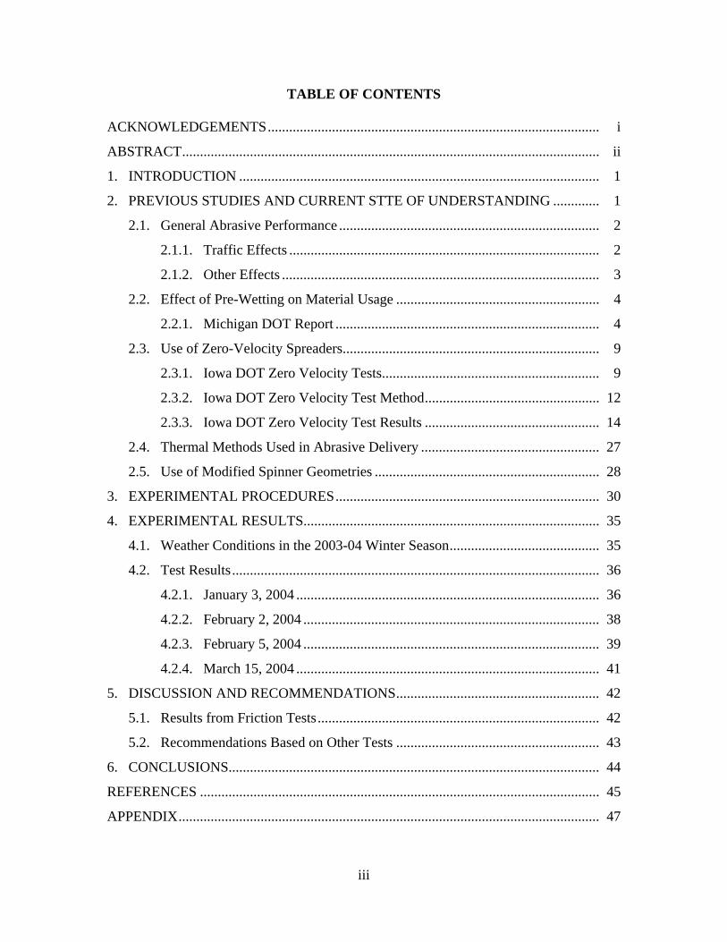
In examining the distribution of materials across the test segments, results are

shown (as noted above) in terms of the percentage of the total collected material found in

a single box or segment of the test area. Figure 2.10 shows the distribution across the test

section for truck A at a delivery rate of 150 lbs per lane mile.

Variation of Material Across Test Segment, Truck A, 150 lbs per Lane Mile

0.00%5.00%

10.00%15.00%20.00%25.00%30.00%35.00%

L Sho

ulder

Far lef

t PL

Mid PL

Mid Righ

t PL

Right P

L

Left D

L

Mid Le

ft DL

Mid DL

Right D

L

R Sho

ulder

Location Across Test Segment

Perc

enta

ge o

f Tot

al

Mat

eria

l A-25-150A-35-150A-45-150

Figure 2.10. Material distribution, Truck A, 150 lbs per lane mile (PL = Passing Lane, DL = Driving Lane)

Figures 2.11 through 2.19 show equivalent results for the remaining 9 truck and

application rate configurations.

19

Variation of Material Across Test Segment, Truck A, 250 lbs per Lane Mile

0%5%

10%15%20%25%

L Sho

ulder

Far lef

t PL

Mid PL

Mid Righ

t PL

Right P

L

Left D

L

Mid Le

ft DL

Mid DL

Right D

L

R Sho

ulder


Perc

enta

ge o

f Tot

al

Mat

eria

l A-25-250A-35-250A-45-250

Figure 2.11. Material distribution, Truck A, 250 lbs per lane mile

Figure 2.12. Material distribution, Truck B, 150 lbs per lane mile

Variation of Material Across Test Segment, Truck B, 150 lbs per Lane Mile

0%5%

10%15%20%25%30%35%

L Sho

ulder

Far lef

t PL

Mid PL

Mid Righ

t PL

Right PL

Left D

L

Mid Le

ft DL

Mid DL

Right DL

Should

er DL


Per

cent

age

of T

otal

M

ater

ial B-25-150

B-35-150B-45-150

20

Figure 2.13. Material distribution, Truck B, 250 lbs per lane mile

Figure 2.14. Material distribution, Truck C, 150 lbs per lane mile

Variation of Material Across Test Segment, Truck B, 250 lbs per Lane Mile

0%5%

10%15%20%25%30%35%40%

L Sho

ulder

Far lef

t PL

Mid PL

Mid Righ

t PL

Right PL

Left D

L

Mid Le

ft DL

Mid DL

Right DL

Should

er DL


Per

cent

age

of T

otal

M

ater

ial B-25-250

B-35-250B-45-250

Variation of Material Across Test Segment, Truck C, 150 lbs per Lane Mile

0%10%20%30%40%50%

L Sho

ulder

Far lef

t PL

Mid PL

Mid Righ

t PL

Right PL

Left D

L

Mid Le

ft DL

Mid DL

Right DL

Should

er DL


Per

cent

age

of T

otal

M

ater

ial C-25-150

C-35-150C-45-150

21

Figure 2.15. Material distribution, Truck C, 250 lbs per lane mile

Figure 2.16. Material distribution, Truck D, 150 lbs per lane mile

Variation of Material Across Test Segment, Truck C, 250 lbs per Lane Mile

0%10%20%30%40%50%60%

L Sho

ulder

Far lef

t PL

Mid PL

Mid Righ

t PL

Right PL

Left D

L

Mid Le

ft DL

Mid DL

Right DL

Should

er DL


Per

cent

age

of T

otal

M

ater

ial C-25-250

C-35-250C-45-250

Variation of Material Across Test Segment, Truck D, 150 lbs per Lane Mile

0%10%20%30%40%50%

L Sho

ulder

Far lef

t PL

Mid PL

Mid Righ

t PL

Right PL

Left D

L

Mid Le

ft DL

Mid DL

Right DL

Should

er DL


Per

cent

age

of T

otal

M

ater

ial D-25-150

D-35-150D-45-150

22

Figure 2.17. Material distribution, Truck D, 250 lbs per lane mile

Figure 2.18. Material distribution, Truck E, 150 lbs per lane mile

Variation of Material Across Test Segment, Truck D, 250 lbs per Lane Mile

0%10%20%30%40%50%60%70%

L Sho

ulder

Far lef

t PL

Mid PL

Mid Righ

t PL

Right PL

Left D

L

Mid Le

ft DL

Mid DL

Right DL

Should

er DL


Per

cent

age

of T

otal

M

ater

ial D-25-250

D-35-250D-45-250

Variation of Material Across Test Segment, Truck E, 150 lbs per Lane Mile

0%10%20%30%40%50%

L Sho

ulder

Far lef

t PL

Mid PL

Mid Righ

t PL

Right PL

Left D

L

Mid Le

ft DL

Mid DL

Far Right

DL

R Sho

ulder

Location Across test Segment

Per

cent

age

of T

otal

M

ater

ial E-25-150

E-35-150E-45-150

23

Figure 2.19. Material distribution, Truck E, 250 lbs per lane mile

There are clear differences observable between the various delivery systems, with

trucks C, D, and E, for example, showing almost no material in the left four segments,

while truck B shows some material in that area, and truck A shows the most material in

that location. However, differences between the delivery systems are best seen by way of

comparisons. Since the systems were being tested to determine how well they could

apply material in a concentrated manner, the ability of each system to deliver material in

a six foot, a nine foot, and a twelve foot wide segment (two, three or four segment

sections respectively) was determined. In each case, the “best” six, nine, or twelve foot

wide segment was chosen. In this context, best was taken to mean that segment in which

the most material was collected. These data are shown in figures 2.20 through 2.24

respectively.

Variation of Material Across Test Segment, Truck E, 250 lbs per Lane Mile

0%10%20%30%40%50%

L Sho

ulder

Far lef

t PL

Mid PL

Mid Righ

t PL

Right PL

Left D

L

Mid Le

ft DL

Mid DL

Far Right

DL

R Sho

ulder


Per

cent

age

of T

otal

M

ater

ial E-25-250

E-35-250E-45-250

24

Figure 2.20. Material concentration for Truck A

Figure 2.21. Material concentration for Truck B

Figure 2.22. Material concentration for Truck C

Truck A 150#

0%10%20%30%40%50%60%70%80%90%

25 mph 35 mph 45 mph

Speed (mph)

% o

f Vol

ume

6 Feet9 Feet12 Feet

Truck A 250#

0%10%20%30%40%50%60%70%80%90%

25 mph 35 mph 45 mph

Speed (mph)

% o

f Vol

ume

6 Feet9 Feet12 Feet

Truck B 150#

0%

10%

20%

30%

40%

50%

60%

70%

80%

90%

25 35 45

Speed (mph)

% o

f Vol

ume

6 Feet9 Feet12 Feet

Truck B 250#

0%

10%

20%

30%

40%

50%

60%

70%

80%

90%

25 35 45

Speed (mph)

% o

f Vol

ume

6 Feet9 Feet12 Feet

Truck C 150#

0%10%20%30%40%50%60%70%80%90%

100%

25 35 45

Speed (mph)

% o

f Vol

ume

6 Feet9 Feet12 Feet

Truck C 250#

0%

20%

40%

60%

80%

100%

120%

25 35 45

Speed (mph)

% o

f Vol

ume

6 Feet9 Feet12 Feet

25

Figure 2.23. Material concentration for Truck D

Figure 2.24. Material concentration for Truck E

The general trends from figures 2.20 through 2.24 are that the higher the speed,

the less material is maintained in the central area of the highway. The exception to this

trend is Truck A at the higher application rate of 250 lbs per lane mile. Additionally, the

general trends do not appear to change substantially depending on the width over which

the material retention is considered. Thus, the material retained in a six foot width is

essentially proportional to that retained in a twelve foot width. Therefore, in any

consideration of comparative behavior between the different delivery systems, it is

sufficient to consider only one of the three widths.

Figures 2.25 and 2.26 show the five different delivery systems’ performance in

terms of how much of the total material was retained in the best six foot width.

Truck D 150#

0%10%20%30%40%50%60%70%80%90%

100%

25 35 45

Speed (mph)

% o

f Vol

ume

6 Feet9 Feet12 Feet

Truck D 250#

0%10%20%30%40%50%60%70%80%90%

100%

25 35 45

Speed (mph)

% o

f Vol

ume

6 Feet9 Feet12 Feet

Truck E 150#

0%

20%

40%

60%

80%

100%

25 35 45

Speed (mph)

% o

f Vol

ume

6 Feet9 Feet12 Feet

Truck E 250#

0%

20%

40%

60%

80%

100%

120%

25 35 45

Speed (mph)

% o

f Vol

ume

6 Feet9 Feet12 Feet

26

Figure 2.25. Material retained in six foot width for all delivery systems, 150 lbs/LM

Figure 2.26. Material retained in six foot width for all delivery systems, 250 lbs/LM

From these figures it is apparent that in general the three zero-velocity systems

retain more material within a narrow section than the two traditional delivery systems. At

the lower application rate, it is clear that the higher the speed of application, the less

material is retained within the narrow area, for all five delivery systems. The degree of

reduction in retained material is somewhat similar for all five systems, although it

appears there is less drop-off with the Swenson system than with the other two zero-

velocity spreaders. At the higher application rate, the reduction of retention with

Percent Retention 150# 6 Foot Width

0%10%20%30%40%50%60%70%80%

25mph 35mph 45mph

SpinnerChuteMonroeSwensonTyler

Percent Retention 250# 6 Foot Width

0%10%20%30%40%50%60%70%80%90%

100%

25mph 35mph 45mph

SpinnerChuteMonroeSwensonTyler

27

increasing speed is less uniform and also smaller. On the basis of these tests, it would

appear that using one of the zero-velocity systems tested in this study provides superior

performance, in terms of material retention, to the two standard delivery systems tested in

this study.

All the data collected by the Iowa DOT during these tests is included, for the sake

of completeness, in the Appendix of this report.

2.4. Thermal Methods Used in Abrasive Delivery A study conducted in Sweden addressed exactly this issue (Hallberg and

Henrysson, 1999). In this study, four different applications of materials were made. The

most traditional was a sand/salt mixture, which consisted of about sand (0 to 8 mm in

diameter) with about 25 kg/m3 of salt (Sodium Chloride) added to prevent caking. The

second traditional material applied was cold aggregate chippings (2 to 5 mm in diameter).

In addition, two novel applications were made. One, termed Hottstone®, applied the

aggregate chippings (2 to 5 mm in diameter) at high temperature (>180º C), using diesel

burners to heat the aggregate just prior to placing it on the road. The second novel

method (termed the Friction MakerTM) applied the (0 to 8 mm) sand with hot (90º C)

water. The aim of both novel methods was to encourage the sand to stick to the snow or

ice covered road surface. All mixtures were applied at rates of 350 kg/lkm per

application.

Both novel methods were able to maintain their friction increase for several days.

This should be contrasted with the two standard methods, which were not able to provide

any lasting friction benefit. As noted by Hallberg and Henrysson (1999): “As early as a

couple of hours after having applied conventional methods, there was no longer any

friction effect left.” These tests were conducted on a road with AADT of 500.

What the Swedish study shows is that abrasives can be applied in such a way as to

provide a lasting friction benefit, but that this requires distinctly non-standard methods.

This method has also been applied with success in Norway. Vaa (2004) reported

on the successful use of this approach. More recently (Vaa and Sivertsen, 2008) this

28

method has been tested on one of the major highways in Norway (National Road E6, in

the Lillehammer region of Norway) and the results indicated that when use of abrasives

was appropriate, the use of this “warm, wet sand” method gave significant friction

increases (and enhanced safety) when applied only four times a day. Clearly this method

works, but to the author’s knowledge, it has not been used in the US or Canada to date.

2.5. Use of Modified Spinner Geometries The purpose of using a spinner to place material on the road has been to spread

the material evenly across the road surface. However, it is far from clear that such a

uniform application is desirable. The argument can be made that in certain circumstances

it is better to windrow the material into a relatively small strip on the road surface, thus

providing a much higher local concentration of material in a limited location on the road

surface.

When using chemicals in a de-icing mode, this windrowing has a significant

advantage. Specifically, it allows for a high chemical concentration in one location, thus

allowing the material applied to melt through the snow or ice cover to the road surface as

quickly as possible. Once the material reaches the road surface, it can melt the interface

between the road and the snow or ice, spreading out horizontally as it does so. This is an

efficient way of applying chemicals in a de-icing mode.

It is less clear whether windrowing abrasives would provide a beneficial effect.

One can envisage how this might happen. The high concentration of abrasives in the

wheel path on a snow or ice covered roadway would require more time to be dispersed by

traffic to the point at which it ceased to be effective in increasing friction. Thus the

primary beneficial effect of such a windrow type application of abrasives would be to

increase the length of time over which an application of abrasives would provide an

increase in friction.

The purpose of the experiments undertaken in this project was to determine

whether two different spinner geometries could provide different friction levels when

used to apply sand on a snow covered pavement. The two geometries are shown in

figures 2.27 and 2.28. The special chute, developed at the Ames DOT garage, is designed

to place the abrasive material directly in the wheel path.

29

Figure 2.27. Sander chute in operation mode

Figure 2.28. Sander chute in by-pass mode

30

The chute has a “trapdoor” in it. When the trapdoor is closed, the material is

deposited in a windrow. When the trapdoor is open, the material drops down onto the

spinner and is deposited in a broadcast manner.

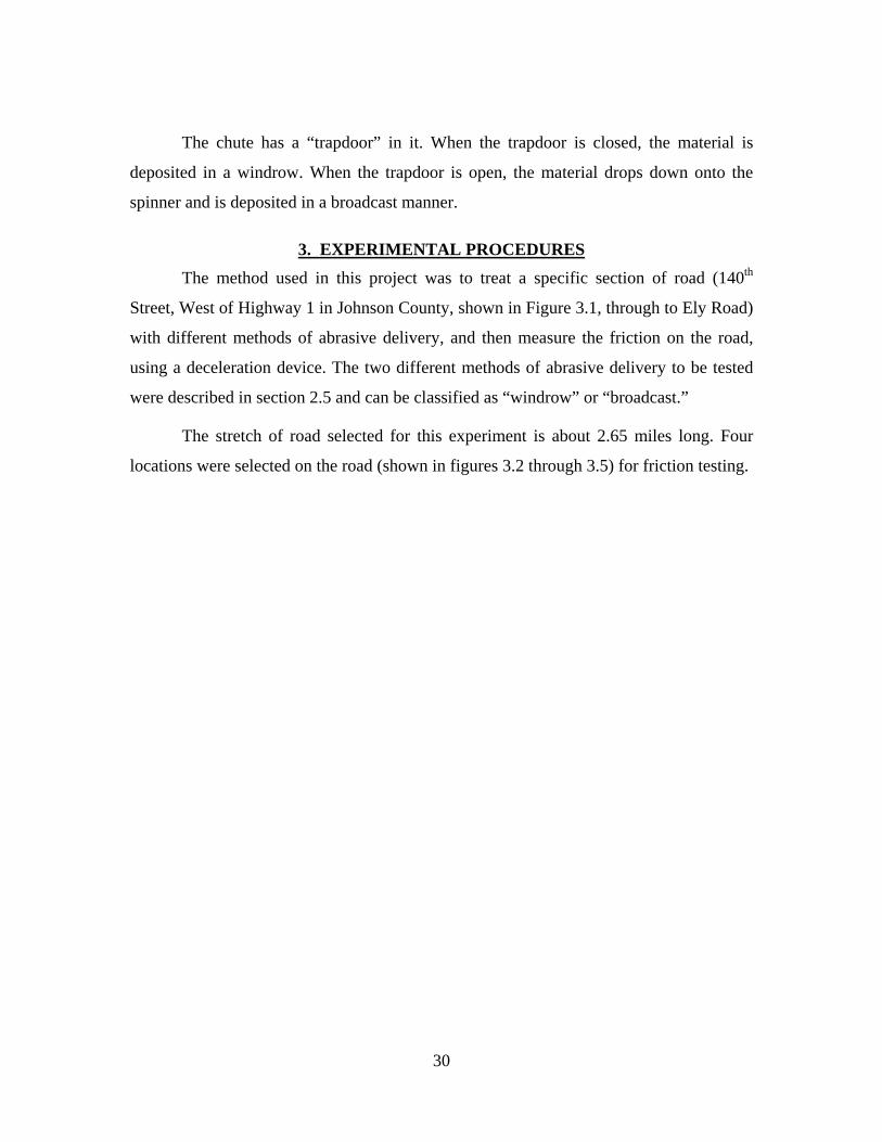
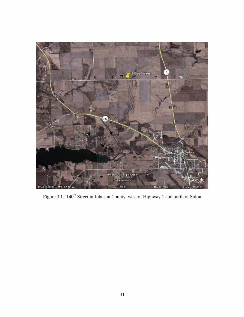
3. EXPERIMENTAL PROCEDURES The method used in this project was to treat a specific section of road (140th

Street, West of Highway 1 in Johnson County, shown in Figure 3.1, through to Ely Road)

with different methods of abrasive delivery, and then measure the friction on the road,

using a deceleration device. The two different methods of abrasive delivery to be tested

were described in section 2.5 and can be classified as “windrow” or “broadcast.”

The stretch of road selected for this experiment is about 2.65 miles long. Four

locations were selected on the road (shown in figures 3.2 through 3.5) for friction testing.

31

Figure 3.1. 140th Street in Johnson County, west of Highway 1 and north of Solon

32

Figure 3.2. First test location, about 0.5 miles west of Highway 1

Figure 3.3. Second test location, about 1.0 mile west of Highway 1

33

Figure 3.4. Third test location, about 1.5 miles west of Highway 1

Figure 3.5. Fourth test location, about 2.0 miles west of Highway 1

34

Testing was conducted using a friction measuring device (a Coralba meter)

mounted in a University of Iowa vehicle (a Chrysler minivan). The Coralba meter worked

by measuring the deceleration of the test vehicle. To measure friction effectively, the

vehicle had to undergo severe breaking from a speed of 35 mph to zero. Thus, particular

care was needed in the testing to ensure that no vehicles were following the test vehicle

when friction testing was being conducted. This is one reason for the selection of 140th

Street as a test location – it is relatively lightly traveled. AADT in 2006 was 620 and in

2002 was 4702.

The goal of the measurement process was to obtain a friction measurement after

the storm had started but before the plow had treated the road. Then, the plow would

come by, using the standard spreader for half the length of 140th street, and the chute

variation for the other half. Ideally, the use of chute and standard delivery methods would

alternate each time the plow went by (thus, if on the first passage, the chute delivery

method was used for the first half of the road, on the second passage the standard

delivery method would be used for the first half of the road, and vice-versa). After the

plow had treated the road, a second set of friction readings would be taken as soon as was

safely possible. Thereafter, friction readings would be taken every 30 minutes, until the

next time the plow came round, at which point the process would start again. Initially, the

goal had been to take friction readings after a certain number of vehicles had passed over

the road, but tracking this proved difficult and it was decided it was unnecessarily

complex. It was planned that traffic counts would be conducted simultaneously with the

testing, but this proved to be infeasible also.

Thus, for any given storm, a series of passes down the road, from east to west,

would be made, with four friction readings being taken on each pass. The time of each

pass start was noted, along with the four friction readings. After the storm, information as

to which delivery method was used when was collected from the truck operator. These

data, along with weather data subsequently collected from National Weather Service sites

(see below) constitute the data set for these experiments.

2 AADT data were obtained from the Iowa DOT Transportation Data Files available on the Internet at : http://www.iowadotmaps.com/msp/traffic/aadtpdf.html accessed on 12/11/2008.

35

4. EXPERIMENTAL RESULTS Tests were conducted during the 2003-04 winter season. In this chapter, the

storms during which testing could be conducted are described first, then the experimental

results are presented.

4.1. Weather Conditions in the 2003-04 Winter Season From a practical viewpoint, the winter season may be considered to run from

November through March. Data from the National Climatic Data Center (NCDC) are

summarized in table 4.1. Days with snow include those days when only a trace of snow

was recorded. Note that February 2004 had 29 days.

Table 4.1. Summary of Weather Data for Winter 2003-04.

Month Days with

Snow

Total Snow

Amount

Days with low

32° or below

Days with high

32° or below

November 2003 3 Trace 18 2

December 2003 10 6.9” 28 8

January 2004 8 7.8” 31 20

February 2004 11 9.9” 26 14

March 2004 6 7.8” 19 0

Table 4.1 indicates that snowfall occurred on 38 days during the winter. However,

a surprisingly high number of these snowfall events involved only a trace of snow or

small amounts of less than 2 inches in depth. Table 4.2 lists those days on which snowfall

of 2 inches or more occurred. This quantity was selected because it is a typical level at

which plowing is required. Note that the high and low temperatures presented in Table

4.2 are for those days, while high and low temperatures during the storms are discussed

in section 4.2 below. The storm on 12.5.03 was marginal on that day, and in fact no data

were collected during that storm. For the other four storms listed, data were collected,

and are presented in section 4.2 below.

36

Table 4.2. Snow Storms during the 2003-04 Winter Season

Date Depth of Snow

(inches)

Low Temperature

(°F)

High Temperature

(°F)

12.5.03 2.0 27 39

1.3-5.04 5.1 -4 39

2.2.04 4.0 20 32

2.5.04 5.2 20 27

3.15-16.04 6.5 26 33

4.2. Test Results Results are presented for each storm during which readings were taken. The data

presented are friction readings expressed as a friction value between 0 and 1. The four

sites at which data are collected are identified in Chapter 3 above as sites 1 through 4.

4.2.1. January 3, 2004 This storm began on Saturday, January 3 between 8 and 9 p.m. Light snow

continued from then until some time between 1 and 2 a.m. on Sunday January 4. Light

snow started falling again at about 6:30 a.m. on Sunday January 4, and continued until

about 7 a.m. on Monday January 5, with very little snow falling between 1 a.m. and 5

a.m. on January 5. Temperatures ranged between 25° and 10.9° F, being in the range of

25° to 20° F through until the evening of January 4, at which time the temperature

dropped significantly.

Ten runs were completed on Sunday January 4, and data are presented in Table

4.3 below. The times indicated are those on which the test vehicle began to move down

140th Street.

37

Table 4.3. Friction Data Collected for January 4, 2004 Storm

Time Location # 1 Location # 2 Location # 3 Location # 4

7:55 a.m. January 4

0.36 0.34 0.34 0.31

8:48 a.m. January 4

0.32 0.31 0.32 0.32

9:44 a.m. January 4

0.29 0.26 0.28 0.29

10:37 a.m. January 4

0.25 0.24 0.28 0.26

11: 35 a.m. January 4

0.26 0.24 0.26 0.25

1:22 p.m. January 4

0.36 0.37 0.34 0.33

2:25 p.m. January 4

0.32 0.31 0.30 0.32

3:28 p.m. January 4

0.29 0.30 0.30 0.28

4:25 p.m. January 4

0.26 0.27 0.26 0.25

5:22 p.m. January 4

0.25 0.23 0.22 0.25

Figure 4.1 shows how the friction varied during this storm.

Variation of Friction with Time, 1.3.04

00.050.1

0.150.2

0.250.3

0.350.4

7:55

8:48

9:44

10:37

11:35

13:22

14:25

15:28

16:25

17:22

Time

Fric

tion

Valu

e

Location # 1Location # 2Location # 3Location # 4

Figure 4.1. Variation of friction with time for storm of 1.3.04

38

4.2.2. February 2, 2004 This storm began on Monday, February 2 between 2 and 3 a.m. with freezing rain,

and temperatures between 30° and 32° F. The rain changed over to snow at about 7 a.m.

This snow continued thereafter until about 2 a.m. on Tuesday February 3. For the most

part, the precipitation after 7 a.m. on February 2 was characterized as light snow,

although there was a period between 1 and 5 p.m. on February 2 when the snow

intensified somewhat (corresponding with reports of fog). From 7 a.m. on February 2

through the end of the storm on February 3 temperatures ranged from 31° to 16° F, with

the temperature dropping significantly after about 10 p.m. on February 2.

Nine runs were completed on Monday February 2, and data are presented in Table

4.4 below.

Table 4.4. Friction Data Collected for February 2, 2004 Storm


8:50 a.m. February 2

0.23 0.22 0.24 0.21


0.21 0.23 0.20 0.22


0.34 0.32 0.33 0.36


0.31 0.30 0.30 0.29

12:45 p.m. February 2

0.32 0.29 0.31 0.27


0.29 0.27 0.28 0.29


0.26 0.25 0.25 0.28


0.24 0.26 0.26 0.25


0.24 0.25 0.26 0.24

39

Figure 4.2 shows the variation of friction during the course of this storm.


0

0.05

0.1

0.15

0.2

0.25

0.3

0.35

0.4

8:50 9:48 10:44 11:37 12:45 14:15 15:12 16:10 17:08

Time

Fric

tion

Valu

e



4.2.3. February 5, 2004 This storm began on Thursday February 5 between11 a.m. and Noon. It continued

as snow or light snow without interruption through about 2 a.m. on February 6. There

was additional light snow from between 5 and 6 p.m. on February 6 through about Noon

on February 7, but no friction measurements were made during this second part of the

storm. Temperatures during the first part of the storm ranged between 27° and 24° F,

while during the second part of the storm (on February 6 and 7) they ranged between 25°

and 12° F.

Eight runs were completed during the storm on Thursday February 5. The

measurements are shown in Table 4.5.

40

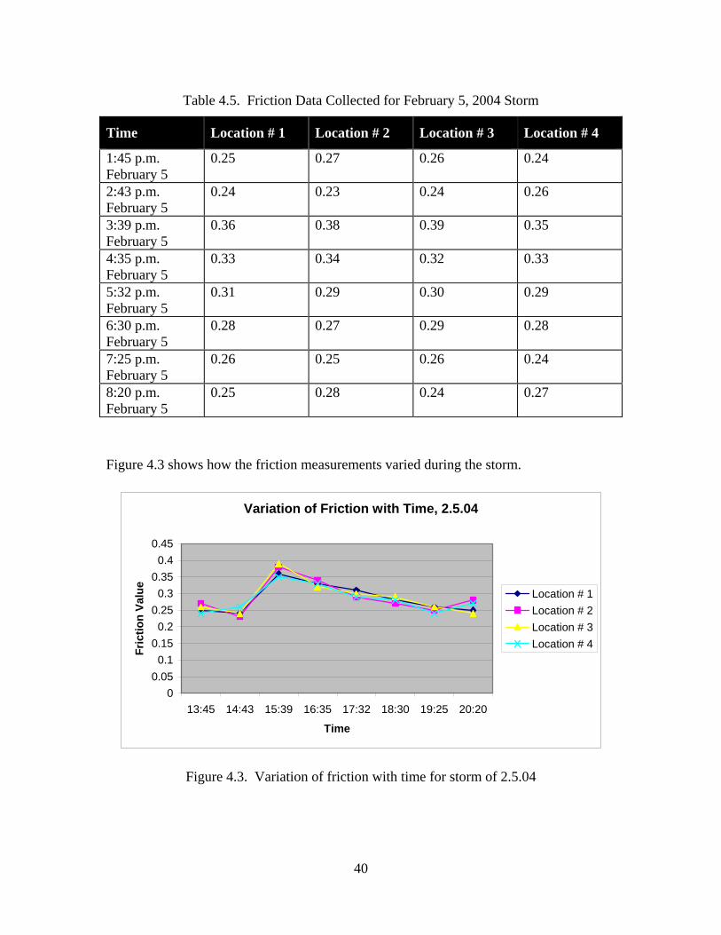
Table 4.5. Friction Data Collected for February 5, 2004 Storm



0.25 0.27 0.26 0.24


0.24 0.23 0.24 0.26


0.36 0.38 0.39 0.35


0.33 0.34 0.32 0.33


0.31 0.29 0.30 0.29


0.28 0.27 0.29 0.28


0.26 0.25 0.26 0.24


0.25 0.28 0.24 0.27

Figure 4.3 shows how the friction measurements varied during the storm.


00.050.1

0.150.2

0.250.3

0.350.4

0.45

13:45 14:43 15:39 16:35 17:32 18:30 19:25 20:20

Time

Fric

tion

Valu

e



41

4.2.4. March 15, 2004 The storm on Monday, March 15 began between 10 and 11 a.m., and ended on

March 16 at about 5 a.m. For the most part, the snowfall was characterized as light snow,

with period s of snow and heavy snow between 11 a.m. and 1 p.m. on March 15. During

the storm, temperatures ranged between 32° and 28.4° F. Additional light snow was

reported between 9:30 p.m. on March 16 and 2:30 a.m. on March 17.

Seven runs were completed during the storm. The collected data are shown in

Table 4.6.

Table 4.6. Friction Data Collected for March 15 2004 Storm.


12.32 p.m. March 15

0.24 0.27 0.22 0.26

1:24 p.m. March 15

0.23 0.23 0.27 0.24

2:17 p.m. March 15

0.31 0.33 0.29 0.34

3:10 p.m. March 15

0.28 0.30 0.29 0.32

4:35 p.m. March 15

0.27 0.31 0.28 0.29

6:45 p.m. March 15

0.24 0.27 0.25 0.27

8:20 p.m. March 15

0.22 0.25 0.26 0.24

Figure 4.4 shows how friction varies during the storm.

42


00.050.1

0.150.2

0.250.3

0.350.4

12:32

:00

13:24

:00

14:17

:00

15:10

:00

16:35

:00

18:45

:00

20:20

:00

Time

Fric

tion

Valu

e



5. DISCUSSION AND RECOMMENDATIONS

5.1. Results from Friction Tests The data collected during the four storms in the 2003-04 winter season (presented

in Chapter 4) were essentially inconclusive insofar as determining whether the spreader

or the chute method of material delivery was more effective at creating a higher level of

friction on the highway. The passage of the plow truck over the road could be clearly

identified from the friction values, and while the truck was not always observed plowing

at that time, in all four storms subsequent conversations with the plow operator confirmed

that the truck did indeed plow 140th Street between test runs for which friction values

increased markedly. It was also confirmed that the truck operator used the standard

spreader for the first half of 140th Street and the chute spreader for the second half in all

cases.

Examination of the data made clear that there was no significant difference in

friction levels between the two locations where materials had been placed with a standard

spreader (locations 1 and 2) and with a chute spreader (locations 3 and 4). Thus, for the

sort of storms observed, there is no benefit or drawback to using the chute configured

43

spreader versus the standard spreader. This is a somewhat negative result, but it

nonetheless shows that either approach can be used for these types of storms with no

drawback. Thus on the basis of this study, no recommendation can be made as to whether

a chute or standard spreader should be used.

5.2. Recommendations Based on Other Tests Three other methods of enhancing friction on roads have been discussed in this

report: pre-wetting of material, the use of zero-velocity spreaders, and the use of thermal

methods when applying the material. For all three methods, there is evidence that the

methods can effectively enhance the placement and/or retention of material on the

pavement surface.

The thermal methods described in chapter 2 (basically either heating material, or

mixing material with near boiling water prior to placing it on the road) have been shown

to be effective when used operationally in Scandinavia. However, the use of heating

systems on trucks here in the United States present significant safety concerns, and thus,

until these safety concerns can be addressed, it is not recommended that these thermal

methods be investigated or considered further.

The use of pre-wetting has been shown to be effective at increasing the quantity

of material retained on the pavement. It is recommended that, whenever possible,

material be placed on the pavement in a pre-wet condition. The best form of pre-wetting

appears to be pre-wetting on the truck at rates of 8 gallons per ton. While pre-wetting

equipment adds to the expense of a plow truck, this expense can be rapidly recovered by

material savings.

The Iowa DOT studies of zero-velocity spreaders showed that such spreaders are

more effective than standard application techniques for placing materials upon the

highway. However, these systems have not, to the author’s knowledge, been tested “side

by side” with pre-wetting systems, so it is unclear whether they perform as well as or

better than such systems. It is recommended that such side by side tests be conducted. It

can be concluded also that zero-velocity systems are superior to standard delivery

systems for material placement.

44

6. CONCLUSIONS A series of field experiments have been conducted to determine whether a

standard or a chute based delivery system provides better friction when used to deliver

abrasives to the road during winter storms. On the basis of these tests, no significant

differences can be found between the two systems.

Reviews of other methods of material delivery have been made, together with an

extensive report of a series of Iowa DOT tests on zero-velocity spreaders. On the basis of

the field testing and the reviews, a number of recommendations with respect to material

delivery systems have been made.

45

REFERENCES Al Qadi, I. L., Loulizi, A., Flintsch, G. W., Roosevelt, D. S., Decker, R., Wambold, J. C.

and Nixon, W. A., “Feasibility of Using Friction Indicators to Improve Winter

Maintenance Operations and Mobility,” Paper No. 04-2751, Proceedings of the

83rd Annual Meeting of the Transportation Research Board, Washington DC

January 11-15, 2004.

Borland, S. L. and Blaisdell, G.L., (1993). "Braking Friction on Sanded Ice,"

Transportation Research Record 1387, pp. 79 - 88.

Comfort, G. and Dinovitzer, A., (1997). "Traction Enhancement Provided by Sand

Application on Packed Snow and Bare Ice: Summary Report," Ontario Ministry

of Transportation Report no. MAT-97-02.

Gray, D. M., and Male, D. H., (1981). Handbook of Snow: Principles, Processes,

Management & Use, Pergamon Press.

Hallberg, S. –E. and Henrysson, G., (1999). "Sanding Tests 1998: Comparison between

Conventional Sanding Methods Using Cold Materials and the Friction MakerTM

and Hottstone® Hot Material Methods," Technical Report no 2105 of the Swedish

National Road Administration (SNRA).

Hossain, M. M., Bajorski, P., and Yang, W.S., (1997). "Frictional Characteristics of

Sand and Sand-Deicer Mixtures on Bare Ice," Transportation Research Record

1585, pp. 30 - 38.

Ketcham, S., Minsk, L.D., Blackburn, R., and Fleege, E., “Manual of Practice for an

Effective Anti-icing Program: A Guide for Highway Winter Maintenance

Personnel,” Report No. FHWA-RD-95-202, Federal Highway Administration,

Washington, D.C., June 1996.

H. Lemon (1975). “1974-1975 Prewetted Salt Report,” Methods Unit of the

Administrative Services Section of the Maintenance Division, Michigan

Department of Transportation.

46

Minsk, L. D. (1998). Snow and Ice Control Manual for Transportation Facilities,

McGraw Hill

Vaa, T. (2004). "Implementation of New Sanding Method in Norway, Transportation

Research Circular E-C063," Proceedings of the Sixth International Symposium on

Snow Removal and Ice Control Technology, Transportation Research Board of

the National Academies, Washington, D.C., pp. 473-486.

Vaa, T. and Sivertsen A., (2008). "Winter Operations in View of Vision Zero,

Transportation Research Circular E-C126," Proceedings of the Fourth National

Conference of Surface Transportation Weather and the Seventh International

Symposium on Snow Removal and Ice Control Technology, Transportation

Research Board of the National Academies, Washington, D.C., pp. 16-26.

47

APPENDIX

This appendix contains the data collected by the Iowa Department of

Transportation during their field testing of material delivery systems. The data were

collected on November 7, 2002.

48

Zero Velocity Tests - November 7, 2002 Truck # A 7-Nov-02 9:10:00 AM Run 1 2:00 Run 8

Truck "A" Number A 29231 Williams Sample Identifier: 1st digit Truck identifier2nd digit Run #

Zero Velocity Spreader Standard Spreader 3rd digit Test section #

Test SectionsTarget Actual Appl. L Shoulder Far left PL Mid PL Mid Right PL Right PL Left DL Mid Left DL Mid DL Far Right DL R Shoulder Total

Run # Speed Speed Rate 9 7 5 3 1 2 4 6 8 10 Weight (gm)

1 25 24.9 150 0 2.1 3.6 5.3 13 15.5 18 6.2 7.4 1.3 72.42 35 33.9 150 0.1 4.2 4.7 10.4 15.3 14.2 7.2 5.4 8.2 8.7 78.43 45 44.2 150 0 8.2 7.4 5.9 15 15.3 13.1 17.6 14.4 12.5 109.44 25 24.7 250 0 3.2 5.1 5.3 13.4 16.7 8 6.1 10 3.4 71.25 35 33.9 250 0 1.7 4.3 6 22.9 23 11.4 10.4 9.8 8.8 98.36 45 42 250 1.2 1.4 5.6 12.5 14.9 9.3 4.6 4.7 6.1 4.7 65

08 25 23.9 150 0 0.3 0 1.3 12.5 12.2 5.8 1.8 3.6 1.5 399 35 33.4 150 0.1 2.46 1.9 4.1 7.3 7.5 7.2 0.97 1.7 0.9 34.13

Target Actual Appl. L Shoulder Far left PL Mid PL Mid Right PL Right PL Left DL Mid Left DL Mid DL Right DL R Shoulder TotalRun # Speed Speed Rate 9 7 5 3 1 2 4 6 8 10 Weight

1 25 24.9 150 0% 3% 5% 7% 18% 21% 25% 9% 10% 2% 100%2 35 33.9 150 0% 5% 6% 13% 20% 18% 9% 7% 10% 11% 100%3 45 44.2 150 0% 7% 7% 5% 14% 14% 12% 16% 13% 11% 100%4 25 24.7 250 0% 4% 7% 7% 19% 23% 11% 9% 14% 5% 100%5 35 33.9 250 0% 2% 4% 6% 23% 23% 12% 11% 10% 9% 100%6 45 42 250 2% 2% 9% 19% 23% 14% 7% 7% 9% 7% 100%

8 25 23.9 150 0% 1% 0% 3% 32% 31% 15% 5% 9% 4% 100%9 35 33.4 150 0% 7% 6% 12% 21% 22% 21% 3% 5% 3% 100%

Weight

Re Do

Re Do For Runs 1 and 2

Percent

49

Zero Velocity Tests - November 7, 2002 Truck # B 7-Nov-02 10:25

Truck "B" Number A 29231 Williams Sample Identifier: 1st digit Truck identifier2nd digit Run #

Zero Velocity Spreader Chute 3rd digit Test section #

Target Actual Appl. L Shoulder Far left PL Mid PL Mid Right PL Right PL Left DL Mid Left DL Mid DL Far Right DL R Shoulder TotalRun # Speed Speed Rate 9 7 5 3 1 2 4 6 8 10 Weight

1 25 23.9 150 0 1.2 1 1.6 22 22 8.7 4.4 5.7 3.4 702 35 33.5 150 0 1.2 3.5 7.7 14.1 10.8 6.5 5.7 5.5 2.7 57.73 45 43.5 150 0 1.4 0.4 1.7 7.6 7.8 7.4 10.1 10.6 6.3 53.34 25 24.9 250 0 1.2 0.3 0.8 8.9 17.2 11.4 4.7 3.7 1.3 49.55 35 33 250 0 0.8 2.4 1.6 14 20.2 18.3 11.1 9.7 4.7 82.86 45 42.9 250 0 2 3.8 13.2 22.1 19 13.3 5.2 6 5.8 90.4

Target Actual Appl. L Shoulder Far left PL Mid PL Mid Right PL Right PL Left DL Mid Left DL Mid DL Right DL Shoulder DL TotalRun # Speed Speed Rate 9 7 5 3 1 2 4 6 8 10 Weight

1 25 23.9 150 0% 2% 1% 2% 31% 31% 12% 6% 8% 5% 100%2 35 33.5 150 0% 2% 6% 13% 24% 19% 11% 10% 10% 5% 100%3 45 43.5 150 0% 3% 1% 3% 14% 15% 14% 19% 20% 12% 100%4 25 24.9 250 0% 2% 1% 2% 18% 35% 23% 9% 7% 3% 100%5 35 33 250 0% 1% 3% 2% 17% 24% 22% 13% 12% 6% 100%6 45 42.9 250 0% 2% 4% 15% 24% 21% 15% 6% 7% 6% 100%

TEST SECTIONWeight

Percent

50

Zero Velocity Tests - November 7, 2002 Truck # C 7-Nov-02 11:20

Truck "A" Number A28463 Bedford Sample Identifier: 1st digit Truck identifier2nd digit Run #

Zero Velocity Spreader Monroe ZV 3rd digit Test section #


1 25 25 150 0 0.2 1.7 0.4 12.5 23.5 4.7 2 3.1 1.5 49.62 35 34.2 150 0 0.2 0.6 1 8.1 15 2.9 1.9 3.7 2.2 35.63 45 45 150 0 0.2 0.4 0.6 7.4 14.1 10.5 5.5 4.7 2.8 46.24 25 25.7 250 0 0.1 0.1 0.3 28.8 38.4 5 1.4 1.6 1.1 76.85 35 35.2 250 0 0.2 0.2 0.3 18.5 37.6 15 5.1 4.1 3.6 84.66 45 43.9 250 0 0.2 0.2 3.1 27.1 32.6 7.1 6.3 5.8 6.8 89.2


1 25 25 150 0% 0% 3% 1% 25% 47% 9% 4% 6% 3% 100%2 35 34.2 150 0% 1% 2% 3% 23% 42% 8% 5% 10% 6% 100%3 45 45 150 0% 0% 1% 1% 16% 31% 23% 12% 10% 6% 100%4 25 25.7 250 0% 0% 0% 0% 38% 50% 7% 2% 2% 1% 100%5 35 35.2 250 0% 0% 0% 0% 22% 44% 18% 6% 5% 4% 100%6 45 43.9 250 0% 0% 0% 3% 30% 37% 8% 7% 7% 8% 100%

TEST SECTIONWeight

Percent

51

Zero Velocity Tests - November 7, 2002 Truck # D 7-Nov-02 12:15

Truck "A" Number A30830 Oakdale Sample Identifier: 1st digit Truck identifier2nd digit Run #

Zero Velocity Spreader Swenson ZV 3rd digit Test section #


1 25 25.2 150 0 0.6 0.5 23.6 19.6 6.1 3.5 1.3 1.9 0.7 57.82 35 36 150 0 0.2 0.4 0.1 5 17.4 8.4 5.8 3.6 1.9 42.83 45 45.6 150 0 0.2 0.9 3.4 11 17.3 12.2 5.2 6.6 1.8 58.64 25 25.8 250 0 0.5 0.6 1.9 7.4 38.6 8.8 3.3 3.5 1.2 65.85 35 37 250 0.1 0.6 0.7 3.2 22.5 36.6 12 5.5 3.9 2.2 87.36 45 45.8 250 0 0.4 0.3 1.4 15.9 32.2 16.8 5.4 5 5.3 82.7


1 25 25 150 0% 1% 1% 41% 34% 11% 6% 2% 3% 1% 100%2 35 34.2 150 0% 0% 1% 0% 12% 41% 20% 14% 8% 4% 100%3 45 45 150 0% 0% 2% 6% 19% 30% 21% 9% 11% 3% 100%4 25 25.7 250 0% 1% 1% 3% 11% 59% 13% 5% 5% 2% 100%5 35 35.2 250 0% 1% 1% 4% 26% 42% 14% 6% 4% 3% 100%6 45 43.9 250 0% 0% 0% 2% 19% 39% 20% 7% 6% 6% 100%

TEST SECTIONWeight

Percent

52

Zero Velocity Tests - November 7, 2002 Truck # E 7-Nov-02 1:20

Truck "A" Number A28079 Sample Identifier: 1st digit Truck identifier2nd digit Run #

Zero Velocity Spreader Tyler 3rd digit Test section #


1 25 25.2 150 0 0.1 0.1 0.6 14.7 29.3 13.7 4.6 2.4 0.9 66.42 35 33.7 150 0 0.2 0 0.5 8.9 14 8.4 3.8 3.6 1.8 41.23 45 43 150 0 1.4 0.1 1.5 10.6 12.9 10.9 11.5 10.2 17.2 76.34 25 24.3 250 0.1 0.5 0.2 0.5 29.7 77.3 45.3 11.3 4.6 1.9 171.45 35 34.2 250 0.1 1.8 0 0.8 26.3 59.2 37.2 18.7 6.8 7.5 158.46 45 43.7 250 0 0.2 0 0 9.1 35.3 38 25.7 17.6 19.1 145


1 25 25 150 0% 0% 0% 1% 22% 44% 21% 7% 4% 1% 100%2 35 34.2 150 0% 0% 0% 1% 22% 34% 20% 9% 9% 4% 100%3 45 45 150 0% 2% 0% 2% 14% 17% 14% 15% 13% 23% 100%4 25 25.7 250 0% 0% 0% 0% 17% 45% 26% 7% 3% 1% 100%5 35 35.2 250 0% 1% 0% 1% 17% 37% 23% 12% 4% 5% 100%6 45 43.9 250 0% 0% 0% 0% 6% 24% 26% 18% 12% 13% 100%

TEST SECTIONWeight

Percent

field testing of abrasive delivery systems in winter maintenance

Documents