FIFTH SEMI-ANNUAL PROGRESS REPORT

NASA GRANT NAG8-790

PROCESS MODELLING FOR MATERIALSPREPARATION EXPERIMENTS

Period of Performance8/1/91 through 1/31/92

Principal Investigator

FRANZ ROSENBERGER

Co-Principal Investigators

J. IWAN D. ALEXANDER

(NASA-CR:189904) PROCESS MODELLING FORMATERIALS PREPARATION EXPERIMENTS SemiannualProgress Report No. 5, 1 Aug. 1991 - 31 Jan.1992 (Alabama Univ.) 38 p CSCL 208

N92-19106

Unclas0071414

Center for Microgravity and Materials ResearchUniversity of Alabama in Huntsville

HuntsvUle, Alabama 35899

Table of Contents

1. Introduction and General Status 2

2. MCT Viscosity Measurements 3

2.1. New Experimental Setup 3

2.2. Low Temperature Measurements 7

2.3. High Temperature Measurements 7

3. TGS Diffusivity Measurements 8

3.1 New Interferometry Cell 9

3.2 High Concentration NaCl Solutions 9

4. MCT Code Development 10

4.1 Introduction 104.2 Solidification: Code Development 11

4.3 The Influence Matrix Method Applied to Convection in a Cylinder 19

5. Presentations and Publications 24

1. Introduction and General Status

The main goals of the research under this grant consist of the development of

mathematical tools and measurement of transport properties necessary for high fidelity modelling

of crystal growth from the melt and solution, in particular for the Bridgman-Stockbarger growth

of mercury cadmium telluride (MCT) and the solution growth of triglycine sulphate (TGS). The

tasks, desribed in detail in the original proposal, include:

development of a spectral code for moving boundary problems,

kinematic viscosity measurements on liquid MCT at temperatures close to the (composition

dependent) melting point, and

diffusivity measurements on concentrated and supersaturated TGS solutions.

The work performed during the fifth six-monthly period of this grant has closely followed the

schedule of tasks.

The code development has progressed well, though some difficulties have been

encountered during this period, which are related to the rate of convergence of our spectral

method. Efforts to remedy this have begun.

The oscillating-vessel technique that we developed for the measurement of the kinematic

viscosity of melts at high temperatures and pressures, has been tested with water and gallium.

Excellent agreement with literature values was obtained. Hence, the technique will be applied to

MCT in the final reporting period.

For diffusivity measurements in (aqueous) solutions we have developed and tested a

technique that overcomes some of the limitations of earlier techniques. During this report period

we have performed extensive tests with concentrated NaCl solutions. Good agreement with

published diffusivity data was obtained. Measurements with TGS will be performed in the final

reporting period.

In the following we will give detailed descriptions of the work performed for these tasks,

together with a summary of the resulting publications and presentations.

2. MCT Viscosity Measurements.

A detailed evaluation of the capillary type viscometer for measurements of HgCdTe melts

was performed during the previous reporting period. Two principal difficulties have been

identified:

1. Larger than expected quantities of material (>500g) are needed in order to build up a

hydrostatic pressure head sufficient to suppress unwanted surface tension effects, such as

the formation of bubbles in the capillary;

2. The assessment of safe cell dimensions for high pressure operation is difficult due to the

complexity of the glassware used in this technique.

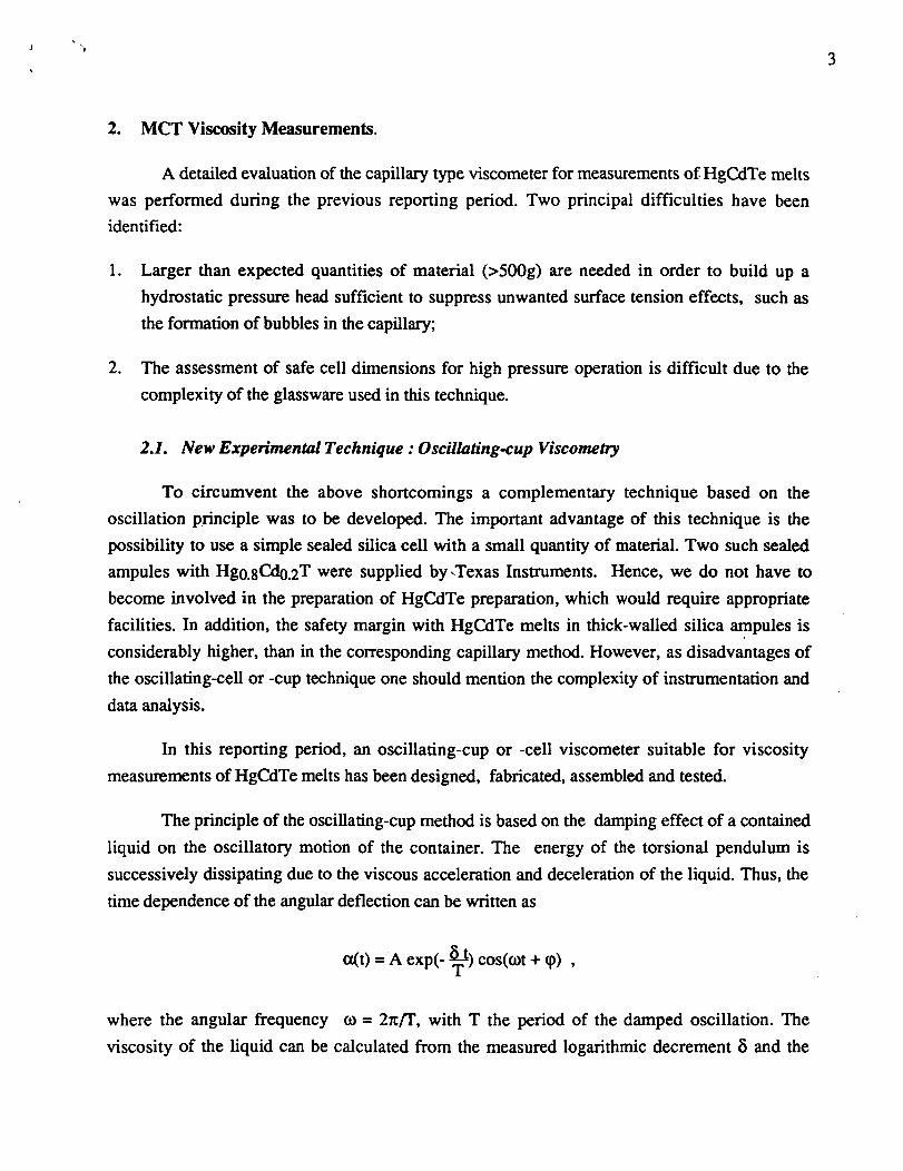
2.1. New Experimental Technique: Oscillating-cup Viscometry

To circumvent the above shortcomings a complementary technique based on the

oscillation principle was to be developed. The important advantage of this technique is the

possibility to use a simple sealed silica cell with a small quantity of material. Two such sealed

ampules with Hgo.gCdo.2T were supplied by-Texas Instruments. Hence, we do not have to

become involved in the preparation of HgCdTe preparation, which would require appropriate

facilities. In addition, the safety margin with HgCdTe melts in thick-walled silica ampules is

considerably higher, than in the corresponding capillary method. However, as disadvantages of

the oscillating-cell or -cup technique one should mention the complexity of instrumentation and

data analysis.

In this reporting period, an oscillating-cup or -cell viscometer suitable for viscosity

measurements of HgCdTe melts has been designed, fabricated, assembled and tested.

The principle of the oscillating-cup method is based on the damping effect of a contained

liquid on the oscillatory motion of the container. The energy of the torsional pendulum is

successively dissipating due to the viscous acceleration and deceleration of the liquid. Thus, the

time dependence of the angular deflection can be written as

ct(t) = A exp(- ̂ ) cos(cot + <p) ,

where the angular frequency to = 27C/T, with T the period of the damped oscillation. The

viscosity of the liquid can be calculated from the measured logarithmic decrement 8 and the

frequency of the oscillation. In addition, the dimensions and density of the liquid, the moment ofinertia and the logarithmic decrement of the empty suspended system are required for the

evaluation

The most reliable and practical equation for viscosity determination with cylindrical

oscillating-cup viscometers is the formula derived by Roscoe (1958)

TipT

where

2 TiH/P

P =7tp 1/2

R

The parameters in these relations are as follows: I is the moment of inertia of the suspendedempty oscillating system, p is the density of the liquid, T is the period of oscillations, R is the

inner radius of the cylindrical cell, H is the height of the liquid in the cell, T| is the viscosity ofthe liquid and 5 is the logarithmic decrement of the empty torsional pendulum. The above set of

equations has to be solved numerically for the viscosity. Means of determining the moment ofinertia I will be described below.

A schematic view of the developed viscometer is presented in Fig.l. Basically, it consistsof a torsional oscillation system enclosed in vacuum. A hardened steel (piano) wire of 0.01"

diameter is suspended from a strain gauge bridge, which, in turn, is suspended from a shaft thatis inserted through a vacuum feedthrough from the outside. A hand knob at the end of this shaftpermits manual induction of an oscillation. At the bottom end, the wire is attached to a flywheel

assembley. This assembley consists of an inertia disk with exchangeable rings. A silicasuspension connects the flywheel to a sealed silica cell for the liquid. A vacuum system(turbomolecular and rotary pumps) can provide a vacuum of the order of 10"̂ Torr in order to

eliminate damping of the oscillations due to friction with air. The furnace used can be controlledwith 0.1 °C resolution from "ambient" to 1300 °C. Three independently controlled heater zonesallow for the adjustment of temperature uniformity of ± 2°C over the length of the silica cell.

Optical techniques are commonly used for measurements of oscillations. In a standardsetup, a laser beam, deflected from a mirror attached to the oscillating assembley is projectedonto a semicircular scale. The amplitude of the oscillation can be determined visually or,alternatively, recorded with a photoconductive linear displacement detector. Instead, we arerecording the torsional amplitude with a simple strain gauge arrangement, and collect and

process the data in a PC.

Figure 2 depicts the torsional motion sensing arrangement. Four strain gauges (Omega

HBM 6/350 LY 11) are glued to the four top stainless steel foil springs of the cross-patternedmetal strip basket. The torsional deformation of the wire over the length of the basket is coupledto the foil springs through the four horizontal spokes of the basket. During the oscillations, thesefoil springs are slightly bent, resulting in a signal from the strain gauges in a bridge arrangementwith a strain gauge amplifier (Omega model DMD). This particular arrangement is ratherselective with respect to torsional oscillations and suppresses signals from horizontal oscillations.

In order to determine a moment of inertia I of the suspended system, the torque constantG of the suspended system and its period of oscillation T needs to be measured. Then I can becalculated from the relation

= G271

= Gco-2

In order determine G and its possible dependence on the suspended weight, we have performed

oscillation experiments with 2 different inertial rings added to the flywheel:Dimensions and mass of the first ring: R 1=34.42 mm, R2=26.60mm, m=152.4g

Dimensions and mass of the second ring: Ri=34.30 mm, R2=26.65 mm, m=261.0 g.

From the relation for the moment of inertia of a ring about its symmetry axis

I=m/2(Ri2+R22),

we calculated

Il=1442.2 gem2 and 12=2462.16 gem2-

The measured angular frequencies were:

Measured frequencies:no rings: wo=1.77 s'1 >

with the first ring attached: wi=0.866 s^1,with the second ring attached: w2=0.699 s'1 •

From IQ = Ii 0)i2/(coo2 - o>i2) and IQ = h £022/(<oo2 - d)22), we obtained IQ = 454 gem2.

Furthermore, the three independently calculated values for the torpue constant were:

G = 454*1.772=1422.3gcm2/sec2, G=(454+1442.2)*0.8662=1422.06gcm2/sec2 and

G=(454+2462.16)*0.6992=1424.8gcm2/sec2'

Since these values agree well with each other, we can assume that load effects can be ignored in

the viscosity evaluation in our apparatus.

The sampling rate of the data aquisition system (DAS) was chosen to be 10/sec, which is

sufficient for accurate recording of oscillations with periods in the range of 5-10 sec. Total data

acquisition times of approximately 1 hour were used. The smallest oscillations which our

detection system can still resolve is about 1 angular degree. Maximum angular amplitudes used

were of the order of 90 degrees. We have carefully evaluated our data for possible nonlinear

effects introduced by the detection system or the suspension wire. However, all data consistently

showed strictly exponential decay of the amplitudes over more than two orders of magnitude; for

details see below. In addition, the signals were quite sinusoidal with no detectable distorsions

due to additional parasitic harmonics. The power spectra of the recorded signals showed only a

single peak and a noise background of a constant magnitude. One third of the total signal trace of

a typical experiment is presented in Fig.3.

Initially, the data were analyzed with a routine that calculated the local amplitudes of the

oscillation as the difference between a local minimum and an adjacent local maximum.

However, the resulting logarithmic plots of the decaying amplitudes showed often a deviation

from a straight line in particular at lower amplitudes; see curve 1 in Fig. 4 obtained with water

(see below). This could be indicative of nonlinear torsional movement, which, in fact, has been

reported in the literature. Another possible cause is a low signal to noise ratio towards the end of

the damped oscillation, were linear, pendulous oscillation contributions become relatively

important. In order to filter the noise, a more complex analysis was performed by fitting a portion

of the data (usually a couple of oscillations) to a sinusoidal function (nonlinear fitting with 4parameters, ao, ai, co, <|>: ao +ai sin(cot-H)))). Amplitudes ai found this way are then plotted on a

logarithmic scale. They exhibit no marked or systematic deviation from a straight line, as

demonstrated by curve 2 in Fig. 4. Consequently, we concluded that no apparent nonlineareffects are present under our experimental conditions.

22. Low Temperature Measurements : Viscosity of Water

We have performed test measurement with water in a cell in air. The data were processedwith Roscoe's formula. The following set of parameters were used : p = 1 g/cm3, R = 1.1 cm, H

= 16.5 cm, I = 1422*(1/0.9)2 = 1755.6 gem2, T = 6.981 s, 8=0.0145. These resulted in

H=0.00943 poise at 22.5 C, which is in excellent agreement with published data.

2.3. High Temperature Measurements: Viscosity of Molten Gallium.

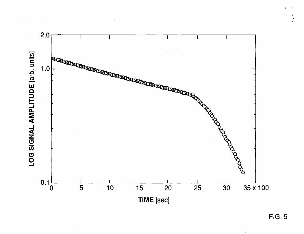
A test experiment with molten gallium was performed to evaluate the heating

arrangement. First, 100.05 g of gallium in form of pellets was loaded into the glass cell. Then,

the logarithmic decrement was measured in air as well as in vacuum. The following values wereobtained: in air: 8=0.00331; in vacuum 8=0.00222. After taking these measurements, the

furnace was powered. In Fig. 5 one can clearly discern the moment when gallium began to melt.

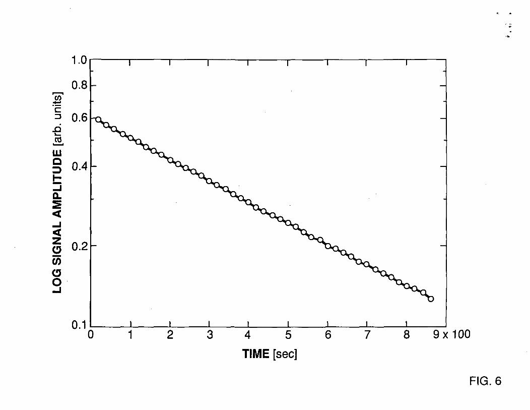
Measurements were made at various temperatures between 27 and 300 °C. Figures 6-8 show the

plots of amlitudes versus time obtained at 200, 250 and 300 °C, respectively. The measurement

at 200 °C was repeated once after a complete temperature cycle and gave the same result within1% . For the viscosity calculations of gallium, the following data were used: co = 0.855 sec'1' p

= 6.1 g/cm3, R = 1.1 cm, H = 4. 2cm, G = 1422 gcm2/sec2. The S's obtained at the various

temperatures, after subtraction of the intrinsic logarithmic decrement of the system (Syac) are

listed in Table 1.

Table 1: Logarithmic decrements versus temperature obtained for galliumTemperature TCI 8

27 0.01406

100 0.01227

150 0.01147

200 0.01125

250 0.01082300 0.01036

The resulting viscosities are plotted in Fig. 9, together with literature data which, assumingArrhenius behavior, follow the relation T) = 0.3567* 1021^.4/T cp \vhile there is good

agreement below 150 °C, there is a deviation of about 10% at the higher temperatures.

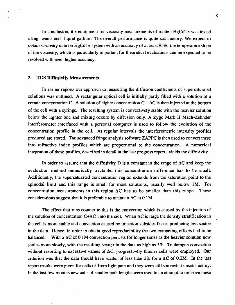
In conclusion, the equipment for viscosity measurements of molten HgCdTe was testedusing water and liquid gallium. The overall performance is quite satisfactory. We expect toobtain viscosity data on HgCdTe system with an accuracy of at least 95%; the temperature slopeof the viscosity, which is particularly important for theoretical evaluations can be expected to beresolved with even higher accuracy.

3. TGS Diffusivity Measurements

In earlier reports our approach to measuring the diffusion coefficients of supersaturatedsolutions was outlined. A rectangular optical cell is initially partly filled with a solution of acertain concentration C. A solution of higher concentration C + AC is then injected at the bottom

of the cell with a syringe. The resulting system is convectively stable with the heavier solutionbelow the lighter one and mixing occurs by diffusion only. A Zygo Mark II Mach-Zehnderinterferometer interfaced with a personal computer is used to follow the evolution of theconcentration profile in the cell. At regular intervals the interferometric intensity profilesproduced are stored. The advanced fringe analysis software ZAPPC is then used to convert theseinto refractive index profiles which are proportional to the concentration. A numericalintegration of these profiles, described in detail in the last progress report, yields the diffusivity.

In order to assume that the diffusivity D is a constant in the range of AC and keep the

evaluation method numerically tractable, this concentration difference has to be small.Additionally, the supersaturated concentration region extends from the saturation point to the

spinodal limit and this range is small for most solutions, usually well below 1M. Forconcentration measurements in this region AC has to be smaller than this range. Theseconsiderations suggest that it is preferable to maintain AC at 0.1M.

The effect that runs counter to this is the convection which is caused by the injection ofthe solution of concentration C+AC into the cell. When AC is large the density stratification in

the cell is more stable and convection caused by injection subsides faster, producing less scatter

in the data. Hence, in order to obtain good reproducibility the two competing effects had to bebalanced. With a AC of 0.1 M convection persists for longer times as the heavier solution now

settles more slowly, with the resulting scatter in the data as high as 5%. To dampen convectionwithout resorting to excessive values of AC, progressively thinner cells were employed. Our

criterion was that the data should have scatter of less than 2% for a AC of 0.2M. In the last

report results were given for cells of 1mm light path and they were still somewhat unsatisfactory.

In the last few months new cells of smaller path lengths were used in an attempt to improve these

results further. Cells of 0.2mm path length completely damped out convection but now the path

length was so small that it was difficult to observe and measure the concentration differences

interferometrically, that is the effective optical path lengths differences between various points inthe cell were very small. Cells of 0.5mm path length gave a good balance between measurabilityand dampening of convection.

Unfortunately cells of less than 1mm path length are not manufactured in standardrectangular shape. Additionally, due to the difficulty of cleaning cells that thin, they are made

with detachable covers and in our experiment this led to problems of seepage between the glassplates. Cells of 1mm path length inserted with microscope slides to reduce the path length werealso tried and here again it was difficult to avoid seepage of the solution between the slides. Allthis meant that the process of obtaining good data had become very difficult and timeconsuming. At this point the decision was made to abandon the optical cells provided by cellmanufacturers and design our own system.

3.1 New Interferometry Cell

An exploded presentation of the new demountable and readily cleanable cell is given inFig. 10. The cell consists of two rectangular windows that sandwich a Viton gasket. Four boltsexcert sufficient pressure onto the windows through two precision-machined brass flanges withhighly planar faces to prevent any leakage. The windows consist of standard microscope slidesthat have been tested interferometrically. The solutions are injected through the open top andviewed through the windows in the flanges. The light path length is equal to the thickness of therubber sheet and can be adjusted by using sheets of different thickness. The results reportedbelow were obtained using rubber of 0.7mm thickness.

With this arrangement all the difficulties associated with this method, as reported earlier,have been overcome. Diffusivities of supersaturated solutions can now be measured with goodreproducibility. An additional benefit is that only fiat glass slides are used here, not glass cellswhich a have greater probability of having stress points. This lack of stress points in the glass

produces fringe patterns of greater uniformity. All this is shown by the reproducibility of thedata which is better than ±1.5%.

32 High Concentration NaCl Solutions

Before application of this technique to TGS, we have performed careful measurementswith saturated and supersaturated solutions of NaCl, for which data are available ion the

literature. Our results are summarized in Table 1. Note that the saturation point at 25 °C is 5.3

10

molar (M). The standard deviations shown are the result of six independent measurements for

each data point.

Table 1. Measured Diffusivities of Concentrated NaCl solutions at 25 °C

Method Used

Previous work [1, 2 & 3]

Diffusivities (cm2/s)

5M

1.584xlO-5

5.2M

1.580xlO-5

5.4M

1.49x10-5

Light path=lmm, AC=0.15M (1.56±0.04)xlO-5

Light path=lmm, AC=0.3M (1.5710.02) xlO'5

Light path=0.7mm,AC=0.2M (1.58±0.02)xlO-5 (1.57±0.02)xlO-5 (1.48±0.02)xlO-5

At this stage we can state that an accurate new interferometric method of measuring

diffusion coefficients of saturated and supersaturated solutions has been developed. The only

other attempt to measure diffusivities of supersaturated solutions was made by Myerson and co-

workers [3]. Our method is not only simpler but provides better reproducibility than the ±3%

achieved in [3]. Work on the diffusivities of supersaturated TGS solutions utilizing this

technique will begin shortly.

References[1] V. Vitagliano and P. A. Lyons, Diffusion Coefficients for Aqueous Solutions of Sodium

Chloride and Barium Chloride, J. Amer. Chem. Soc., 78 (1956) 1549.

[2] J.A. Rard and D.G. Miller, The Mutual Diffusion Coefficients ofNaCl-H2O and CaC^-

H2O at 25 °Cfrom Rayleigh Interferometry, J. Solution Chem, 8(1979) 701.

[3] Y.C. Chang and A.S. Myerson, The Diffusivity of Potassium Chloride and Sodium

Chloride in Concentrated, Saturated and Supersaturated Solutions, AIChE J., 31 (1985)

890.

4. MCT Code Development

4.1 Introduction

During the last semi-annual period work was completed on the solution of the moving

boundary problem for axisymmetric solidification in the absence of convection. In addition, a

code which solves for axisymmetric convective flow in a circular cylinder using a Chebyshev

11

pseudo-spectral method together with an influence matrix method was also completed. The

solidification code development is described in section 4.2 and the axisymmetric convection code

is described in section 4.3.

4.2 Solidification: Code Development

Governing equations and boundary conditions

The governing equations and boundary conditions are described in terms of a cylindrical

coordinate system with the orgin located at the centerline and the top of the ampoule. Variables

are put in dimensionless form by scaling lengths with the ampoule radius R and defining the_ ___slc __

dimensionless temperature as T=(T - Tc)/(Th - Tc) where Th - Tc is the (fixed) temperature

difference between the top and bottom of the ampoule

(1)

(2)

(3)

where subscripts m, c, and a refer to melt, crystal and ampoule, respectively. Here, the Pecletnumber, Pe =VaR/oc, represents the dimensionless transition rate of the ampoule, and Va, R and

a are, respectively, the growth velocity, ampoule radius and thermal diffusivity.

Boundary conditions

T(r,0) = l, (4)

T(r,A) = 0, (5)

3T(0, z)dr

= 0, (6)

(7)

12

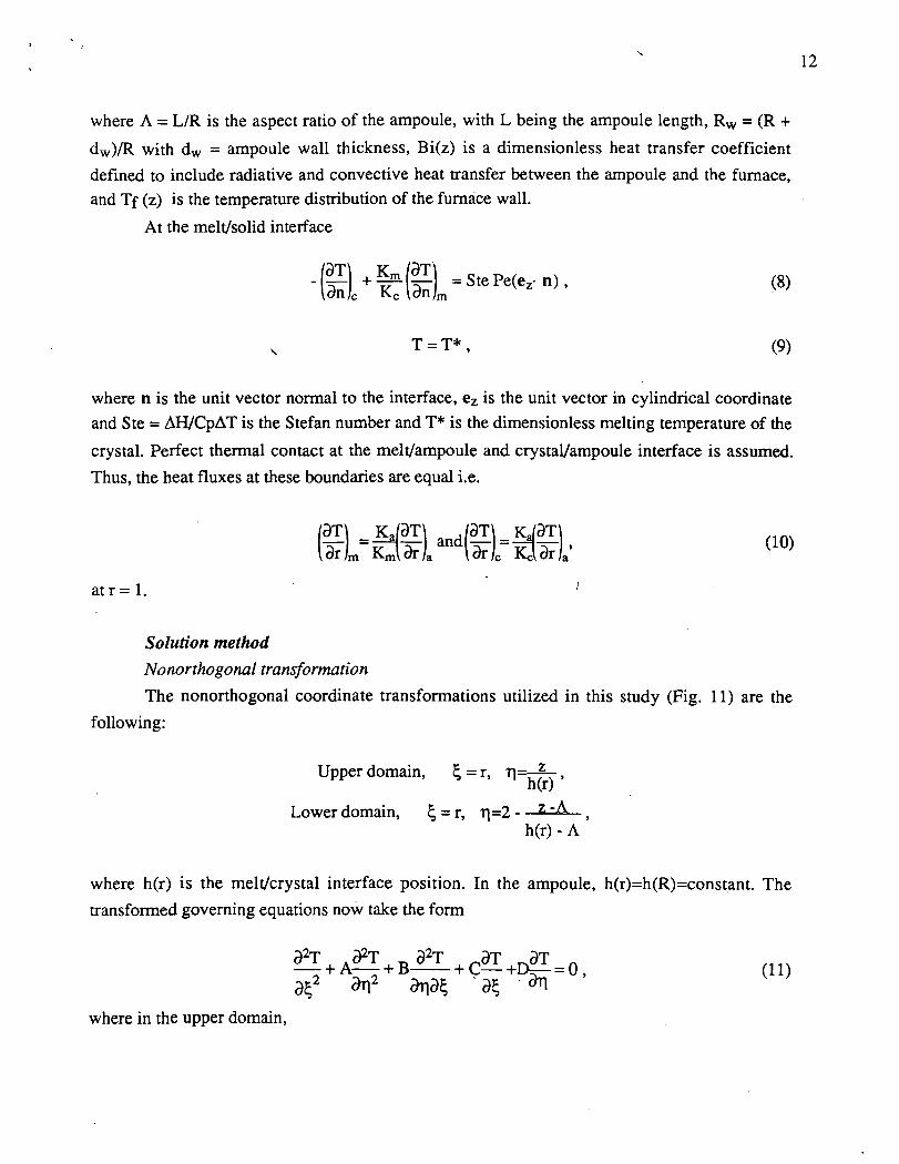
where A = L/R is the aspect ratio of the ampoule, with L being the ampoule length, Rw = (R +

dw)/R with dw = ampoule wall thickness, Bi(z) is a dimensionless heat transfer coefficient

defined to include radiative and convective heat transfer between the ampoule and the furnace,and Tf (z) is the temperature distribution of the furnace wall.

At the melt/solid interface

\^-\ =StePe(e z-n) ,c \dn/m

(8)

= T*, (9)

where n is the unit vector normal to the interface, ez is the unit vector in cylindrical coordinate

and Ste = AH/CpAT is the Stefan number and T* is the dimensionless melting temperature of the

crystal. Perfect thermal contact at the melt/ampoule and crystal/ampoule interface is assumed.

Thus, the heat fluxes at these boundaries are equal i.e.

3T)m K•m dr

and /3T

a t r= l .

(10)/a

Solution method

Nonorthogonal transformation

The nonorthogonal coordinate transformations utilized in this study (Fig. 11) are the

following:

Upper domain, £=r , Ti=-f-,h(r)

Lower domain, = r, r\=2h(r)-A

where h(r) is the melt/crystal interface position. In the ampoule, h(r)=h(R)=constant. The

transformed governing equations now take the form

(ID

where in the upper domain,

13

h2

Here, Pe should be taken as Pem and Pea, respectively, for the melt and ampoule.

In the lower domain,

A = -

2(ri-2)3h--- =—

h-A 5r

-A / h-A9r ^(h-A) h-A

where Pe should be taken as Pec and Pea respectively in the crystal and ampoule. The boundary

conditions are also subject to the coordinate transformations.

Pseudospectral discretization

The total solution domain is divided into four subdomains (Fig.l) and for each subdomain

the equation (11) is discretized using a Chebyshev-collocation method. The Chebyshev

polynomial expansion for the dependent variables is

MJST(12)

where tj(x) = cos(iarccos(x)), tj(y) = cos(j arccos y), and x and y are defined by the

transformations given in Fig. 1 1 for each of the subdomains. The Gauss-Lobatto collocation

points are(i-l) , -and

The Chebyshev collocation derivative of a function T(x,y) can be represented as

14

m= lD'>T(xp,yj),

p=i

ardyi q=l

(14)

(15)

(15)

\ m,n= y wm , v ) ,x y " p'-'q'

(17)

(18)

q=l

where the expressions for Dx, Dy, Dxx, Dyy and Dxy are given by Ouazzani[l].For large m, n,the Chebyshev collocation differentiation can be efficiently implemented by using FFT's (FastFourier Transforms), which eliminates the use of expensive matrix multiplication involved with

PGCR method for finite difference preconditioningIn the present investigation, the preconditioning solution method for spectral equations

involves finite difference preconditioning imbedded within each iteration. This allows theproblem to retain spectral accuracy while using a finite-difference method to solve a relatedauxiliary problem. For this purpose, we need a finite difference discretization for thepreconditioned version of equation (11). The following second order accurate finite differenceformulas are employed for the entire non-uniform grid:

9x/idxi+1 j-M-1

f. f.-1 f.

(dx-+dx+1)dx. dxdx+1(19)

15

The resulting finite-difference equation takes the form:

Aqjtoj + Aeijfo-n j +Awij((>i_lij+Anij<j>iij+1 +ASJ j (frj

+Awn..(bi . . , +Aws..<}x . . . =R. (20)IjU-l.J+l IjM-l.J-l 1J v '

where Ry is the residual of equation (11) at node (ij) and ty1) is the difference in the variable T

evaluated at the current and previous steps. This leads toA <|> = R. (21)

The finite-difference matrix A is a nine-diagonal coefficient matrix. It is approximated by

incomplete factorization i.e. A=L U , where L* is a lower triangular matrix and U* is an upper

Triangular matrix, and the factors are easy to calculate. The approximate factors L and U may

have the sparsity structure of the original matrix. The solution for equation (21) is

straightforward since it consists of forward substitution

U*> = (L*)-lR, (22)

followed by a backward substitution, -<|> = (U*)-l(L*)-lR. (23)

The subsequent approximations are obtained via

T n M - 1 =T n +X<j>, (24)

where X is a relaxation parameter. Unfortunately, such an iteration scheme generally converges

slowly, so an acceleration technique must be added. Alternative acceleration techniques which

have been developed are conjugate direction methods. For sparse symmetric positive-definite

linear systems the preconditioned conjugate residual method is one of the best. However,

equation (11) is far from symmetric, therefore, in the present investigation the preconditioned

generalized conjugate residual (PGCR) method is the chosen acceleration technique since it was

developed specifically for nonsymmetric systems.

The PGCR procedure is as follows:

Initialize

TO

A<)>0 = R°

16

Iterate_ (Rm. LPm)

(LPm,LPm)

= T™ + am+1Pm

Rm+l _ Rm . ou+1 Lpm

= Rm+l

(LPJ.LPJ)

j=0

The scalar a is chosen to minimize the Euclidean norm of the residual. The |3's are

orthogonality coefficients and result from the orthogonality property for the conjugate residualversion. The practical calculation only requires the following condition to terminate the iteration

rPTO+l TTTl

max '- - -^ < e , (26)

where we took e = 10~7 .

The PGCR method is an attractive iterative method for solving non-symmetric systemsince the iteration cannot break down, it is stable and the minimization increases the convergencerate considerably. We compared the PGCR method to a Conjugate Gradient Squared (COS)method and a Strongly Implicit Procedure (SIP). For all these methods, we also used incomplete

factorization to solve the preconditioned problem. The results show that PGCR method is moreefficient in terms of CPU time.Outer iteration

Having computed the new values of temperature, an outer-loop iteration is required toupdate the melt/solid interface h(r) at which the computed temperature is equal to Tmelt. One

scheme to update the interface shape is Newton's method

9h "! Fi, (27)

17

where Fj = TJJ* - Tmeit, here Ty* is the calculated temperature at the Lth interface location.

However for Newton's method, it is difficult to guarantee the outer iteration convergence for all

cases. Therefore as an alternative to Newton's method, an interpolation scheme is used to update

the interface. In the present study, the new interface is located by the following linear

interpolation:ifTm<T i jandTm>T i, j+1

(28)

The outer-loop iteration is continued until the following convergence criterion is satisfied:

ER = mahL+1 - <<, f (29)hL+1

where we took e = 10"4 .

Results and discussion

For the purposes of comparison of our method with that of Adornato and Brown [2] (for

cases in which convection did not influence the interface shape) we have carried out numerical

simulations for the growth (in the absence of convection) of a gallium-doped germanium (Ga:Ge)

alloy in a vertical Bridgman system. (Thus, our computed interface shapes, which are for

solidification in the absence of convection could be compared with theirs). The calculations for

Ga:Ge growth are presented separately for the two furnaces and the different ampoule. For

a heat-pipe furnace, the changes in the heat transfer coefficient between ampoule and three

zones of furnace are modelled by the function

Bi(z) = ( 0 3 { 1 + tanh[ci(zc - c2 - z)f}+l+ tanh[-ci(zc + c2 -z)]) ,

where zc is the location of the mid-plane of gradient zone. The Bio is the value of Biot number in

the cold zone, C3 sets the ratio between the Biot numbers in the hot and cold zone, GI is the slope

of the transition in Bi (z) between the isothermal zones and the adiabatic region, and c2 is the

half of the dimensionless length of the adiabatic zone. The furnace wall temperature is modelled

by the functionTf (z) = 0.5 { 1 + tanh[ 12(0.5 - z/A)]},

18

where the constants in this expression have been fit to the measured wall temperature of the

furnace. For details of the thermophysical properties and growth conditions the reader is referred

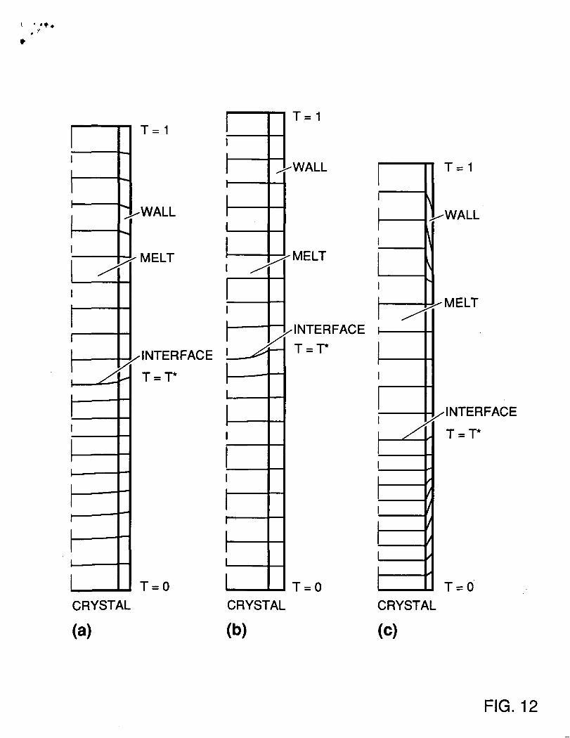
to [2].For a heat pipe furnace and a boron nitride ampoule, the temperature field is shown in

Fig.l2a. The difference between the thermal conductivities of the melt, crystal and ampoule

cause the melt /crystal interface to be convex with respect to the melt and results in the

temperature decreasing radially adjacent to the phase boundary. The mismatch in thermal

boundary conditions between the adiabatic and hot zones of the furnace causes a second set of

radial gradients with the hottest temperature located at the ampoule wall. Fig.l2b depicts thetemperature field using a quartz ampoule (in a heat pipe furnace) which decreases the

conductivity of the ampoule to a factor of 14 lower than the melt. As seen by Adornato and

Brown, the ampoule wall takes up most of the radial temperature difference required to transport

heat in the system. Thus, the interface is flatter, and the radial temperature gradients near the

interface are smaller. Larger radial temperature gradients occur near the intersection of the

adiabatic and hot (cold) zones.

The constant gradient furnace is modelled by using a constant Biot number over the entirelength of the ampoule and specifying the furnace temperature profile as

T f = l - z / A .

The isotherms are almost flat, the large radial gradients that arise at the intersection of adiabatic

and hot (cold) regions in the heat-pipe furbace is eleminated, and the deflection of themelt/crystal interface is large as indicated seen in Fig. 2.c.

In addition to the work described above, we have started to add convection in the melt

phase. The biggest problem encountered to date appears to be that of convergence rates which atpresent are excessively slow even with the finite difference preconditioning.

Future Work

Work planned for the next six monthly period includes the incorporation of melt

convection into the model. Based on our experience with convergence rates for the problem of

convection in a cylinder (see section 4.3) using the influence matrix method (without

preconditioning) the prospects of obtaining an efficient solution method for the coupled

convection-solidification problem are presently not good. We will thus continue to investigate

convergence acceleration techniques for spectral methods.

References

[1] J. Ouazzani, Mtthode Pseudo-spectrale pour la Resolution des Equations d'un Melange de

Gaz Binaire, These, Universitie de Nice (1984).

[2] P.M. Adornato and R.A. Brown, J. Crystal Growth 80 (1987) 155.

19

4.3 The Influence Matrix Method Applied to Convection in a Cylinder

Governing equations

For an axisymmetric system, in cylindrical coordinates the heat and momentum transportequations in stream function - vorticity form may be written as

^-+u-VT = aVT, (1)3t

(2)at

O«-» r** *) r+f

a \i/ i a\i/ a \i/ »~—-i--r=- + — = T(&

where T represents temperature, We the azimuthal component of the vorticity, y the stream

function, t time, a the thermalxdiffusivity, v the kinematic viscosity, p the coefficient of thermal

expansion, gz the axial component of the gravitational acceleration, u the velocity vector, anduZjur the axial and radial components of the velocity, respectively. The "~" indicates a

dimensional variable.

The stream function \|/ in eqn. (3) is defined by

(4,r oz r oz

and the azimuthal component of vorticity is defined by

5e = - (5)

For an axisymmetric system the two other components of vorticity are identically zero.

Due to the extra diffusive component in eqn. (2) coe/r2, which arises in cylindrical

coordinates, an alternative variable S = ro)0 must be solved for so that the discretization in time is

consistent (details given below). Therefore

as -a ~as r _— + ur— + uz— --^ = v — --Jr— + — — +rpgz— , (6)K6

20

and

are solved for in place of eqn.s (2) and (3).

(7)

Equations (1), (6), and (7) are solved inside a cylinder of radius R and height H. Due to

axisymmetry, the boundary condition

ara? = 0,

r = 0(8)

is applied at the centerline. Dirichlet, Neumann, or Cauchy boundary conditions may be applied

for the temperature at the top, bottom, and side of the cylinder.

The no-slip condition for the fluid velocity at the top, bottom, and side of the cylinder

results in the boundary conditions

3z z=- H=°' §Z ~ 2 ~ i-a'0- IF2

= 0,r = 0

(9)

for the stream function. Since the value of the stream function is arbitrary to within a constant, its

value is set to zero at the top, bottom, and side of the cylinder. This combined with the condition

of no penetration for the fluid velocity at the centerline determines the value of the stream

function at the centerline to be zero.

Because of axisymmetry, S=0 at the centerline. As is the case for vorticity in the stream

function - vorticity formulation, the boundary conditions for S at the other three boundaries are

not predeterminable.

The general approach of scaling the velocities by a characteristic velocity U, the times by

a characteristic time t, and lengths by a characteristic length L results in the nondimensional

equations

a2e a2e

ar2-v2 -. ^2a \i/ ^ a\i/ a \j/-\ -7 T /)r

RePr

(10)

(H)

(12)

21

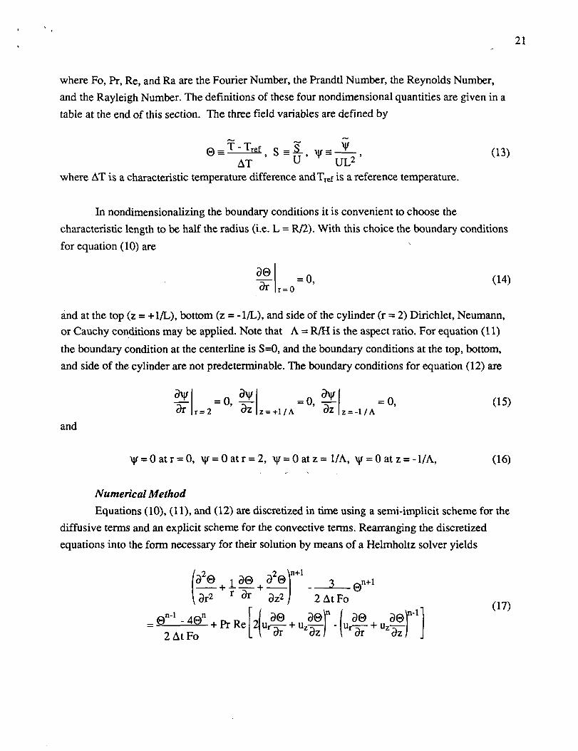
where Fo, Pr, Re, and Ra are the Fourier Number, the Prandtl Number, the Reynolds Number,

and the Rayleigh Number. The definitions of these four nondimensional quantities are given in a

table at the end of this section. The three field variables are defined by

0 =

where AT is a characteristic temperature difference andTref is a reference temperature.

(13)

In nondimensionalizing the boundary conditions it is convenient to choose the

characteristic length to be half the radius (i.e. L = R/2). With this choice the boundary conditions

for equation (10) are

r = 0= 0, (14)

and at the top (z = +1/L), bottom (z = -1/L), and side of the cylinder (r = 2) Dirichlet, Neumann,or Cauchy conditions may be applied. Note that A = R/H is the aspect ratio. For equation (11)

the boundary condition at the centerline is S=0, and the boundary conditions at the top, bottom,

and side of the cylinder are not predeterminable. The boundary conditions for equation (12) are

= 0• ~\r=2 02 z = + l / A

-0.* = 0,z = -l

and

r = 0 at r = 0, v = 0 at r = 2, \|/ = 0 at z = I/A, \if = 0 at z = -I/A,

(15)

(16)

Numerical Method

Equations (10), (11), and (12) are discretized in time using a semi-implicit scheme for thediffusive terms and an explicit scheme for the convective terms. Rearranging the discretized

equations into the form necessary for their solution by means of a Helmholtz solver yields

n+l

(17)

2AtFo

22

, (18)n+l= S^4SfL + Re|2jU]

2 At Fo Pr

where the integers n-1, n, n+1 indicate the number of the time step.

Due to the lack of boundary conditions for equation (18), the method of the matrix of

influence is used for the solution of the momentum part of the problem, that is equations (18) and

(19). In the method of the matrix of influence first a preprocessing stage must be completed. In

this stage a set of elementary solutions are calculated. These elementary solutions are defined by

o S; i oSi o Si1 OT 9z2 2AtFoPr

with boundary conditions

_ _(20)

(21)Sj(Tli) = 0, r = 0,

and2 2

3 \J/i i d\lf; 3 \ifi—-r-£- + —-=si>3r2 r ^ 9z2 J

with boundary conditions

Vj = 0, atr = 0, r = 2, z = 1 z = ± (23)A A

where 8y is the Kronecker delta, 'Hi are the collocation points that lie on the boundary of the

computational domain, F represents all of the boundary except for the centerline, andFMi is the

special matrix of influence subset of P. The final two steps of the preprocessing stage are the

generation of the matrix of influence, and then to take its inverse. The matrix of influence is

TU6FMI , (24)

where n is the outward pointing unit normal at each boundary. Due to the occurence of At in

equation (20) the preprocessing steps must be repeated if the size of the time step is changed.

23

At each time step seven stages are completed. The first stage is solution of

* ^^S i 3S 3 S

2AtFoPr

. S»*-4S» + Re j / a s + Uz|S . 2_S_u> I 38 + 9S . 2S2AtFoPr H 9r dz r / I Br 9z r

with boundary conditions

S=0,

The second stage is solution of

= 0,r = 2, z= -, z = -A A

2xv "^ 2^*o \|/ i dxj/ d \lt ^— - + — ̂ =S

with boundary conditions

= 0, atr = 0,r = 2 ,z= -L,z = ^-A A

X"** _

Using V from the second stage, in the third stage h is generated:

(25)rRa

Re Pr 9r '

(26)

(28)

In the fourth stage 'ki is generated:

The fifth stage is the solution of equation (18) with boundary conditions

(29)

(30)

li) = 0, r = 0,

In the sixth stage the stream function at the (n+l)* time step is generated by solving equation

(19) with boundary conditions

\|/n+1=0atr = 0, \|/n+1=0atr = 2, \|/"+1 = 0 at z = I/A, \j/n+1 =0a t z = -I/A. (32)

Finally, in the seventh stage the true values of Sn+1 on the boundary are calculated by evaluating

the left-hand side of equation (19).

24

Non-Dimensional Groups

Fourier Number

Prandtl Number

Reynolds Number

Rayleigh Number

Fo = ai /L2

Pr = v/a

Re = U L / v

Ra = (3gATL 3 / va

5. Presentations and PublicationsFrom the work carried out under this grant the following papers have been published,

accepted for publication or are in preparation for submission for publication:

1. A. Nadarajah, F. Rosenberger and J. I. D. Alexander, Modelling the Solution Growth ofTriglycine Sulfate in Low Gravity, J. Crystal Growth 104 (1990) 218-232.

2. F. Rosenberger, J. I. D. Alexander, A. Nadarajah and J. Ouazzani, Influence of ResidualGravity on Crystal Growth Processes, Microgravity Sci. Technol. 3 (1990) 162-164.

3. J. P. Pulicani and J. Ouazzani, A Fourier-Chebyshev Pseudo-Spectral Method for SolvingSteady 3-D Navier-Stokes and Heat Equations in Cylindrical Cavities, Computers andFluids 20 (1991) 93.

4. J. P. Pulicani, S. Krukowski, J. I. D. Alexander, J. Ouazzani and F. Rosenberger,Convection in an Asymmetrically Heated Cylinder, Int. J. Heat Mass Transfer (accepted)

5. F. Rosenberger, J. I. D. Alexander and W.-Q. Jin, Gravimetric Capillary Method forKinematic Viscosity Measurements, Rev. Sci. Instr. (submitted).

6. A. Nadarajah, F. Rosenberger and T. Nyce, Interferometric Technique for DiffusivityMeasurements in (Supersaturated) Solutions, in preparation.

In addition to the above publications, the results of our work have been presented at thefollowing conferences:

1. "Commercial Numerical Codes: To Use or Not to Use, Is This The Question?" presentedby J.I.D Alexander at the Microgravity Fluids Workshop, Westlake Holiday Inn,Cleveland Ohio, August 7-9, 1990.

2. "Fluid Transport in Materials Processing" presented by F. Rosenberger at the

Microgravity Fluids Workshop, Westlake Holiday Inn, Cleveland Ohio, August 7-9,1990.

25

3. "Influence of Residual Gravity on Crystal Growth Processes," presented by F.

Rosenberger at the First International Microgravity Congress, Bremen, September (1990).

4. "Modelling the Solution Growth of TGS Crystals in Low Gravity", presented by A.

Nadarajah at the Eighth American Conference on Crystal Growth (July 15-21, 1990, Vail,

Colorado).5. "Modelling the Solution Growth of TGS Crystals in Low Gravity", presented by J. I. D.

Alexander at the Committee on Space Research (COSPAR) Plenary Meeting (June 26 -

July 6, 1990, The Hague, Netherlands).

6. "An Analysis of the Low Gravity Sensitivity of the Bridgman-Stockbarger Technique",

presented by J. I. D. Alexander to the Department of Mechanical Engineering at Clarkson

University, April, 1991.

7. "Residual Acceleration Effects on Low Gravity Experiments". A 3-lecture series

presented by J. I. D. Alexander at the Institute de Mechaniques des Fluides de Marseilles,

Universitd de Aix-Marseille III, Marseille, France, January, 1991.

8. "Measuring Diffusion Coefficients of Concentrated Solutions, presented by A. Nadarajah

at the Fifth Annual Alabama Materials Research Conference, Birmingham September

1991.

9. "Modelling Crystal Growth Under Low Gravity", presented by A. Nadarajah at the

Annual Technical Meeting of the Society of Engineering Science, Gainesville, November

1991.

STARTER KNOB

O-RING

STRAIN GAUGE

VACUUM PORT

SUSPENSION WIRE

INERTIA RING

VIEW PORT

SILICA SUSPENSION ROD

INCONELTUBE

FURNACE

SILICA CELL

FIG. 1

SHAFT TO HAND KNOB

STRAIN GAUGE

FOIL SPRING

SUSPENSION WIRE

FIG. 2

lllllllllllll'lll"

200 400 600

TIME [sec]

800 1000

FIG. 3

1.0000

V).»-«"c

0.1000UJQ3

0.

Z 0.0010oCO

0.00010 400 800 1200

TIME [sec]

1600 2000

FIG. 4

c3

•

.Q

UJQ

2CO(3o

10 15 20

TIME [sec]

25 30 35x100

FIG. 5

1.0

0.8

0.6

&LUO 0.4

0.2CO(3O

0.10 4 5

TIME [sec]

8 9x100

FIG. 6

10.000

-j 1.000

LUQ

E! 0.100

35 0.010(5O

0.0010 10 15 20

TIME [sec]

25 30 35x100

FIG. 7

10.00c

.a

^O

H-J0.

<

<

2CO

0.10

0.010 10 15

TIME [sec]

20 25x100

FIG. 8

CLO

2.2

2.0

1.8

1.6

CO

8 1-4en

1.2

1.0

0.80 50

O THIS WORK

• LITERATURE

100 150 200

TEMPERATURE [°C]

250 300

FIG. 9

FIG. 10

• ' .**•-

RELATIONSHIP BETWEEN PHYSICAL ANDCOMPUTATIONAL DOMAINS

Rw

I

z = h(r)

MELT

4=r•y

J}=W)

A-h(r)

CRYSTAL

I1 Rw

x =2^-1

y = 2ri - 1

y = 2ri - 1

y =Ti-1

y =Ti-1

For each

-1<x<1- 1 < y < 1

FIG. 11

^

^-^

\ —

1 — • — -

^

—

/**

^^

•—

T=1

/WALL

-MELT

/INTERFACE

T T*= \

T 0

I

I

^

-*

I

•

.x-

^

/

T=1

-WALL

-MELT

^INTERFACE

T = T*

I

I

T n

^x

!

s

/

/////

^

CRYSTAL CRYSTAL CRYSTAL

(a) (b) (c)

T = 1

-WALL

MELT

•INTERFACE

T = T*

T = 0

FIG. 12