figur e 1.2. richmond drive, cambuslang, glasgow
TRANSCRIPT

figur e 1.1. Boy playing football in Govan, Glasgow, Scotland, 2008.
figur e 1.2. Richmond Drive, Cambuslang, Glasgow.

Denmark
Japan
SwedenFinland
Canada
India
New Zealand
China
Argentina
Peru
0
0.2
0.4
0.6
0.8
0.1
0.3
0.5
0.7
0.1 0.2 0.3 0.4 0.5 0.6 0.7
Gini coefficient
Inte
rgen
erat
ion
al e
arn
ings
cor
rela
tion
UnitedStates
United Kingdom Chile
figur e 1.3. Intergenerational earnings correlation and inequality.
figur e 1.4. Intergenerational education correlation and income inequality.
Sweden
NorwayDenmark
United States
United Kingdom
ItalyBrazil
Peru
0
0.2
0.4
0.6
0.8
0.1
0.3
0.5
0.7
0.2 0.3 0.4 0.5 0.6
Gini coefficient
Inte
rgen
erat
ion
al e
duca
tion
cor
rela
tion

intr oduction 7
who died b etween 2000 a nd 2012 ha ve left est ates wi th a n a verage val ue o f £416,000, more than fi ve times the average estate value in England in this period. If the standard mobility estimates are correct, the chance that a family like this could maintain a hig h social status over seventeen generations is va nishingly small.3
Pepys is not the only rare surname to maintain a surprising presence and persistence a t t he u pper r eaches o f En glish s ociety. Th e p henomenon is r e-markably common. Sir Timothy Berners-Lee, OM, KBE, FRS, FREn g, FRSA, the creator of the World Wide Web, is a des cendant of a family that was r ich and prominent in e arly-nineteenth-century England. But, f urther, t he name Berners is descended from a Norman grandee whose holdings are listed in the Domesday Book of 1086. Sir Peter Lytton Bazalgette, the producer of the TV show Big Brother and chair of the Ar ts C ouncil England, is a des cendant of
3 Th e most fa mous Pepys, Samuel, did no t contribute himself to this distinguished lin-eage, as he has no known descendants.
figur e 1.5. John Hayls, Samuel Pepys, 1666.

intr oduction 9
in all t he societies for which we construct surname estimates—medieval En-gland, modern England, the United States, India, Japan, Korea, China, Taiwan, Chile, and even egalitarian Sweden—is between 0.7 and 0.9, much higher than conventionally estimated. Social status is inherited as strongly as any biological trait, suc h as heig ht. Figure 1.6 co mpares conventional estimates o f mobility (for income and years of education) with those yielded by surname measures.
Even t hough t hese rates of intergenerational mobility are low, t hey have been eno ugh t o p reclude t he f ormation o f a ny p ermanent r uling a nd lo wer classes. Mobility is co nsistent across generations. Although it may take ten or fi ft een generations, social mobility will e ventually erase most ec hoes of initial advantage or want.
Counterintuitively, t he a rrival o f f ree p ublic ed ucation in t he la te nine-teenth century and the reduction of nepotism in g overnment, education, and private fi rms have not increased social mobility. Nor is there any sign that mod-ern economic growth has done so. Th e expansion of the franchise to ever-larger groups in t he nineteenth and twentieth centuries similarly has had no eff ect. Even the redistributive taxation introduced in t he twentieth century in co un-
0
0.2
0.4
0.6
0.8
1
Swed
enJap
an
South
Kore
a
United K
ingd
om
United St
ates
ChileIn
dia
China
Inte
rgen
erat
ion
al c
orre
lati
onConventional
Surname
figur e 1.6. Conventional versus surname estimates of status persistence.

sweden 21
Swedish Surnames
Surprisingly, despite Sweden’s reputation as a mo del social democracy, a c lass of nobles is v ery much alive and functioning. Th e country has a f ormal guild of noble families, the Riddarhuset (House of Nobility) (fi gure 2.1). Th o ugh noble families have existed since medieval times, the modern Riddarhuset was created in 1626. From 1668 to 1865, it functioned as o ne of the four governing estates of the kingdom, analogous to the House of Lords in En gland. Since 200 3 the Riddarhuset has b een a p rivate in stitution t hat ma intains t he r ecords o f t he Swedish nob le families, and lobbies on t heir b ehalf. In sp ite o f Sweden’s ad-vances in g ender eq uality, o nly men v ote in t he Ridda rhuset, a nd o nly s ons transmit titles to their off spring.
t a bl e 2.1. Estimates of status persistence rates by occupations, Sweden, 1700–2012
1 700–1900 1890–1979 1950–2012
Attorneys — — 0.73Physicians — 0.71 0.80University students 0.80 — 0.67Royal Academy members 0.88 0.75 0.83
figur e 2.1. Th e Riddarhuset, headquarters of the Swedish nobility, in downtown Stockholm.

22 ch apter t w o
0
1,000
2,000
3,000
2,500
1,500
500
3,500
1600 1700 1800 19001650 1750 1850 1950 2000
Nu
mbe
r of
fam
ilies
Noble families createdSurviving families
figur e 2.2. Th e history of ennoblement in Sweden: families enrolled in the Riddarhuset.
Th e families enrolled in t he Riddarhuset occupy three hierarchical ranks: in des cending o rder, t hese a re co unts, ba rons, a nd “untitled” nob ility. M ore than two thousand families have been enrolled, though only about seven hun-dred have li ving representatives.4 Th e timin g o f t hese ennob lements is sum-marized in fi gure 2.2. As the fi gure shows, almost all extant noble families were enrolled before 1815: indeed, a large fraction of all noble families was created in the period 1658–1721, when Sweden’s territories encompassed Finland, Estonia, and some north German states. From 1680 onward the nobility gradually lost its privileges, starting with the reclamation by the crown in 1680 of much of the land granted to nobles in previous years. By 1866 the nobles had no economi-cally signifi cant privileges.
When Swedish families were enrolled in t he Riddarhuset, they typically adopted a ne w sur name em bodying st atus elemen ts suc h as gyllen (g old), silfver (silver), adler (eagle), leijon (lio n), stjerna (st ar), creutz (cr oss), a nd ehren (honor). Th us we get names like Leijonhufvud, Gyllenstjerna, Ehrensvärd, and Adlercreutz. Rosencrantz and Guildenstern, the two unfortunate Danish nobles in Shakespeare’s Hamlet (written around 1600) have forms of two com-
4 Riddarhuset 2012.

24 ch apter t w o
(1707–78), Ander s C elsius (1701–44), J öns J akob B erzelius (1779–1848), a nd Olaus Rudbeckius (1630–1702). Typical examples of these surnames now are Aquilonius, Arrhenius, Berzelius, Boethius, and Cnattingius.
Only a small f raction of the modern population bears such latinized sur-names. Of those dying between 2000 a nd 2009, f or example, only 0.5 percent bore a sur name ending in ei ther -ius or -eus. However, in t he late nineteenth and early twentieth century, signifi cant numbers of people adopted newly cre-ated latinized surnames. Figure 2.4 shows that of men born 1810–1990 the pro-portion with latinized surnames doubled over time.
To avoid including newly adopted surnames, the latinized surnames em-ployed here are restricted to those that existed before 1800. One quick way to identify suc h lo ng-established sur names is t o co nsider o nly la tinized sur -names held by forty or more people in 2011.7 Th ey are overwhelmingly held by those who inher ited them f rom their parents as o pposed to adopting them, perhaps b ecause o f t he restrictions imposed on name c hanges in t he Name Regulation Law (släktnamnsförordningen) of 1901 and the Naming Law of 1982,
7 Because a ne w latinized name only recently adopted would not have time t o grow to have forty holders by 2011, this criterion narrows names to those in existence much earlier.
DeathsBirths
0.0
0.8
0.6
0.4
0.2
1810 1850 1890 1930 1970 2010
Per
cen
tage
of m
ale
birt
hs
and
deat
hs
figur e 2.3. Percentage of aristocratic surnames at death for men born 1810–2009.

sweden 25
which now requires the Swedish Tax Agency to approve all surname changes. Th ese surnames constitute 0.2 percent of the current population.8 Th e share of these o lder la tinized sur names in t he p opulation is c lose t o st able b etween 1810 and 1989.
Th e most common Swedish surnames are patronyms, surnames formed from th e fi rst na me o f t he fa ther a nd endin g in -son. Th ese w ere t he p re-dominant type of surname in preindustrial Sweden. A sample of seventeenth-century parish marriage records, for example, shows that 93 percent of those who married bore such patronyms.9 In early Sweden, such patronyms changed from g eneration t o g eneration. I n t he eig hteenth a nd ninet eenth cen turies, their use declined, and families adopted more permanent surnames. Th e 1901 Name Regula tion L aw called f or e ach fa mily t o ha ve a sur name t hat w ould remain unchanged across generations.
Th e decline of patronyms has continued to this day. Figure 2.5 shows esti-mates by twenty-year periods of the number of Swedish men b orn with and
8 As Watson and Galton famously demonstrated, rare surnames over many generations tend to either die out or survive at a relatively higher frequency (Watson and Galton 1875).
9 FamilySearch, n.d.
All latinizedLatinized pre-1800
0.0
0.1
0.2
0.3
0.4
0.6
0.5
1810 1830 1850 1870 1890 1910 1930 1950 1970 1990
Perc
enta
ge o
f mal
e bi
rth
s
figur e 2.4. Percentage of latinized surnames at death for men born 1810–1979.

26 ch apter t w o
dying wi th a pa tronym as sur name. Aft er t he y ear 2000, o nly 40 p ercent o f males who died in Sweden bore a patronym. But for those dying before age 10, the share was even lower, approximately one-quarter.10
We can observe the sources of this decline if we consider the percentage of patronyms occurring among all men b orn in 1950–51 dying by 2009. Of t his cohort, half of those dying before age 10 but only a third of those dying between ages 50 and 59 had a patronym. By implication, nearly one-third of men born with patronyms changed their surnames, with most o f the changes occurring by age 30. Th us, although patronyms in Sweden are associated with low social status, we have to be careful when using them to measure social mobility, since such patronyms are only selectively retained by the modern population.
Nina Benner, a reporter for Swedish Radio, tells a nicely illustrative story from her own family of how such surname changes took place. Her grandfather and his four brothers changed their surname from Andersson to Benner in 1916, when her grandfather was sixteen. His eldest brother was studying to become a physician, and his professor made it clear that Andersson wasn’t a suitable name
10 Th is trend is due in part to a substantial increase in children born to immigrants in this period. Of males b orn in 2000 w ho died b y 2009, o ne in t en had a M uslim fi rst name, and another one in ten had a name suggesting an immigrant parent.
-son deaths-son birthsLund- and -berg births
0
100
80
60
40
20
90
70
50
30
10
1800 2000198019601940192019001880186018401820
Perc
enta
ge o
f mal
e bi
rths
and
dea
ths
figur e 2.5. Percentage of men with surnames ending in -son, by date of birth and death.

sweden 27
in that profession. Th e name Benner stems from the small village of Bennebo, where her great-grandfather grew up.
Th e incidence of other Swedish names, however, remains constant among men in diff erent age cohorts. As fi gure 2.6 shows, of men born in 1950–51, the percentage holding surnames ending in -berg (mountain) was the same among those dying before age 10 as among those dying aft er age 50. Th es e topographi-cal surnames can be used as a standard for measuring social mobility rates.
Surnames and Current Earnings and Wealth
Since the two sets of elite surnames, noble and latinized, were established before 1800, we w ould exp ect, gi ven t he ra pid ra tes o f s ocial mob ility r eported f or Sweden in t he c urrent and previous generations, t hat t hese sur names would have regressed completely to mean social status. Th ey would not diff er in any way from the average surname in Sweden. Th eir connotation of exalted status would have been totally lost.
One way we can measure the status of diff erent surnames, and also the dis-tribution of status, in modern Sweden is from tax records. Th is information is
-berg
-son
0
60
40
20
50
30
10
0 60504030
Age at death2010
Perc
enta
ge o
f mal
e de
aths
figur e 2.6. Percentage of men born in 1950–51 with surnames ending in -berg and -son, by age at death.

Leijonhielm, Anna Örnbacken 26 320,400 10,131Leijonhielm, Larsson, May Backvindeln 63 283,000
Leijonhufvud, Cecilia Banérgatan 46 2 tr 481,700 467,543Leijonhufvud, Madeleine Basaltgrand 10 340,100
Leijonhufvud, Margareta Bergsmarksvagen 4 1 tr 1,576,800 100,317Leijonhufvud, Louise Blackebergsbacken 5 tag 144 119,400 1,080,423Leijonhufvud, Eld Blanchegatan 18 4 tr 336,700Leijonhufvud, Margareta E C A Halsingehöyden 11 247,000 2,082,476Leijonhufvud, Christina Hogbergsgatan 11 279,200Leijonhufvud, Elisabeth Kommendorsgatan 28 573,500Leijonhufvud, Jenny Krukmakargatan 67 lag 0015 523,000Leijonhufvud, Alice Langelandsgatan 10 318,200 289Leijonhufvud, Susanna Manhernsgatan 13 bv 283,000Leijonhufvud, Sven Märdvagen 34 362,100 54,519Leijonhufvud, Elisabet Märdvagen 34 308,200 1,256Leijonhufvud, Eric Mybrogatan 64 648,000 40,340Leijonhufvud, Gustaf Mybrogatan 68 t tr 239,500 152,518Leijonhufvud, Titti Odengatan 23 5 tr 322,700Leijonhufvud, Ewa K S Ragvaldsgatan 21 4 tr 534,300 123,020Leijonhufvud, Ruth Sigrid G Rindogatan 42 289,300Leijonhufvud, Fredrik Rälambsvägen 10 A 1,224,800 23,100Leijonhufvud, Elizabeth Rälambsvägen 10 A 3 tr 667,800
figur e 2.7. Sample of published tax returns for Stockholm, 2008.
Noble surnamesAnderssonLatinized surnames
0
35
30
25
20
15
10
5
0–249 250–299 300–399
Income (thousands of kroner)
400–599 600–1199 1200
Perc
enta
ge o
f sur
nam
e gr
oup
figur e 2.8. Distribution of taxable income within surname groups, 2008.

0Titled noble Untitled noble Latinized Lund- -son
2
1
3
4
5
6
Rel
ativ
e re
pres
enta
tion
0.25
1.00
0.50
2.00
4.00
8.00
1940 1950 1960 1970 1980 1990
Birthdate
0.69
0.72
0.710.77
Rel
ativ
e re
pres
enta
tion
Titled noble
LatinizedUntitled noble
-son
figur e 2.9. Relative representation of surname types among attorneys, 2012.
figur e 2.10. Relative representation of surname types among attorneys, by birthdate, 2012.

32 ch apter t w o
changed t heir na mes in t his wa y, t he estima ted co rrelation co uld b e signifi -cantly higher than the true correlation.) Th e average intergenerational correla-tion reported for attorneys in table 2.1 is 0.73 for the three elite surname groups. Th e estimated correlations do diff er by surname group, but because the num-bers of attorneys in each surname group are typically less than fi ft y, these varia-tions in estimated correlations could easily stem from chance alone.
physi c ia nsA second source for measuring social mobility rates is the list of physicians in Sweden registering fi rst between 1890 and 2011, which covers four generations. Starting wi th c urrently r egistered p hysicians, w e s ee in fi gure 2.11 the s ame diff erences in r elative r epresentation o f sur names t hat w e s ee a mong a ttor-neys. Th e surnames of the three elite groups of the eighteenth century are over-represented r elative t o t heir sha re o f t he p opulation. P atronyms a re gr eatly underrepresented.
Analyzing surname types for Swedish physicians is complicated by the fact that a subst antial proportion of currently registered physicians in S weden are of foreign origin. Physicians with a medical licen se from any other European
0.0Titled noble Untitled
nobleLatinized Lund- -son
0.5
Berg-
1.0
1.5
2.0
2.5R
elat
ive
repr
esen
tati
on
figur e 2.11. Relative representation of surname types among registered Swedish physi-cians, 2011.

sweden 33
Union country can register in Sweden without further required training. Th us in 2007, almost one in fi ve of all physicians registered in Sweden were trained abroad, including Swedes who attended foreign medical s chools. But of those registering fi rst in 200 7, excluding Swedes trained in f oreign medical s chools, two of every fi ve were foreign.13 One consequence is that even surnames such as Lund-, which have an average representation among attorneys, are under-represented among physicians.
To correct for this complication and calculate the relative representation of Swedish sur name typ es a mong S wedish-born p hysicians in S weden, i t is as-sumed that all f oreign physicians were registered in 1980 or later, and that the relative representation of the surnames Lund- and Berg- averaged one between 1980 and 2011. Th ese assumptions imply that in this cohort, only 70 percent of all physicians are Swedish born—a reasonable estimate. Th e overall domestic phy-sician population for these years is calculated accordingly. For the years before 1980, it is assumed that all registered physicians in Sweden were Swedish born.
Figure 2.12 shows relative representation of the four surname types—titled noble, untitled noble, latinized, and patronyms—among physicians in t hirty-
13 “Every Other Doctor in Sweden from Abroad” 2009.
0.1
1.0
0.5
0.3
2.0
4.0
8.0
1900 1920 1940 1960 1980 2000
Birthdate
Rel
ativ
e re
pres
enta
tion
Titled noble
Latinized-son
Untitled noble
figur e 2.12. Relative representation of surname types among Swedish physicians, 1890–2011.

34 ch apter t w o
year cohorts, by registration date, beginning in 1890. To make clearer what is happening with the patronyms, a loga rithmic scale is us ed in fi gure 2.12. All three groups regress toward the mean, but their rate of regression is again very slow among all co horts. Figure 2.13 shows the best-fi tting relative representa-tion for all t hose in t he three high-status groups across the four generations. Th e estimated persistence rate in this case is 0.74, and the fi t, as can be seen, is good. Th e rate of regression to the mean was no fast er in the past thirty years than in earlier years. To a fi rst approximation, it was the same as in the years be-fore 1980.
Th e corresponding persistence rate for the patronyms is similarly high, at 0.74. Again, however, we must be cautious about the estimate for patronyms. Because of t he abandonment of patronyms, w hich was lik ely more common among the upwardly mobile, the intergenerational correlation estimated here may o verestimate t he p ersistence o f st atus a mong t hose wi th patronym sur-names. However, the persistence rate estimated for this group is the same as for the three elite surname groups.
Th us the representation of surnames among both attorneys and physicians in Sweden suggests a similar pattern: social mobility in Sweden is much slower than t he conventional estimates sug gest, e ven for very recent generations. A
1
2
4
8
1900 1920 1940 1960 1980 2000
Birthdate
Rel
ativ
e re
pres
enta
tion
Titled nobleUntitled noble
LatinizedFit
b � 0.74
figur e 2.13. Estimated persistence rate for Swedish physicians with elite surnames.

sweden 35
second surprising fi nding from the surname distribution of Swedish physicians is that not only are true social mobility rates slower than conventionally esti-mated, but they are no faster now than they were in the early twentieth century. Th e enlargement of the political franchise and the institutions of the extensive welfare state of modern Sweden, including free university education and main-tenance subsidies t o st udents, ha ve do ne no thing t o incr ease ra tes o f s ocial mobility.
Educational Mobility, 1948–2012
Th e ineff ectiveness of free university education in increasing social mobility is borne o ut b y pa tterns o f sur name distr ibution a mong uni versity grad uates, even in recent decades. Figure 2.14, for example, shows the relative representa-tion of the surname groups among those completing master’s theses at Uppsala University f rom 2000 t hrough 2012. Taking sur names o f t he f orm Lund- or Berg- as ha ving an average representation, the noble and latinized surnames, largely originating before 1800, are again overrepresented by 60 t o 80 percent. Th e most common patronyms appear at half their expected representation.14
14 See again Clark 2013 for details of these calculations.
0.0Titled noble Untitled
nobleLatinized Berg- -son
0.5
Lund-
1.0
1.5
2.0
2.5R
elat
ive
repr
esen
tati
on
figur e 2.14. Surnames of Uppsala students submitting master’s theses, 2000–20 12.

sweden 37
lation being observed at universities, is 0.72 for the titled noble surnames, 0.75 for the untitled noble surnames, and 0.57 for the latinized surnames.
However, b ecause t he s ample size f or t hese sur names a t Uppsala in t he years 1942–66 is small , t here is signifi cant s ampling er ror in t hese estimates. Combining these groups into one elite implies an overall intergenerational cor-relation across these two generations of 0.66. Yet the two subsequent genera-tions of students matriculated aft er major reforms in 1977 that greatly expanded access to universities. Tuition is now free, and grants and loans are available to students to cover living costs.
For the patronym surname group, here estimated on the basis o f the sur-names Andersson, Johansson, Karlson, and Nilsson, the implied intergenerational correlation, 0.87, is e ven lower. Th e caveats detailed above for such estimates apply here also.
Educational Mobility, 1700–1908
Th ere are good data available on the surnames of Lund attendees for the period 1666–1908: sources include a register of all students for 1732 through 1830 and detailed biographies from a number of the student nations that all students had
1
0.5
2
4
8
16
0.25
01940 1950 1960 1970 1980 1990 2000 2010
Rel
ativ
e re
pres
enta
tion
Titled noble
LatinizedUntitled noble
-son
figur e 2.15. Relative representation of surnames at Uppsala University, 1948–2012.

38 ch apter t w o
to enroll in. F or Uppsala there is co mplete registry data for the period 1477–1817, but data from only one student nation for the period 1817–1902.
Figure 2.16 sho ws t he r elative r epresentation o f la tinized sur names a t Lund by thirty-year cohorts, starting in 1700. In the fi rst generation observed, 14 percent of Lund students had la tinized surnames, compared with an esti-mated 0.13 percent of the general population. Such names were thus 122 times more common among students than in t he general population. Th e share of latinized surnames among students fell to 1.1 percent by 1880–1909. Th ey were 5.3 times as frequent among Lund students as among the general population. Th e pace o f t his dec line in r epresentation implies a hig h p ersistence of t his group, however. Th e persistence rate estimated for 1700–1909 is 0.7 8, assum-ing t hat uni versity st udents r epresented t he t op 0.5 p ercent o f t he st atus distribution.
One complication in calc ulating persistence is sur name changing. If stu-dents born with the surname Andersson were changing this to Wigonius as they entered t he university eli te, t hen p ersistence would b e exag gerated. Th e bio-graphical sources for some of the student nations at Lund and Uppsala, which list the parents’ surnames for most students, allow us to estimate the fraction of latinized surnames newly adopted in e ach generation. Figure 2.17 shows what
2
4
64
128
32
16
8
11700 19401910188018501820179017601730 1970 2000
Rel
ativ
e re
pres
enta
tion
Lund
UppsalaCorrelation 0.78
Correlation 0.84
figur e 2.16. Relative representation of latinized surnames, Lund and Uppsala university students, 1700–2012.

sweden 39
percentage o f st udents in e ach g eneration inher ited ra ther t han ado pted a latinized sur name.17 B etween 1730 and 1819, 96 p ercent o f st udents acq uired latinized names by inheritance. However, in the period 1820–1909, that propor-tion fell to 88 percent (even though, by design, these are all surnames that ex-isted before 1800).18 Th e tendency of new members of the university-educated elite in nineteenth century Sweden to switch to such latinized surnames means that t he p ersistence rate estimates for t hese years represent an upper b ound. Th e true persistence rate is likely lower. Th us there is no good evidence of any decline in t he p ersistence ra te f or st atus b etween p reindustrial a nd mo dern Sweden, despite the enormous institutional changes that have taken place.
A more elite group of academics t han Lund and Uppsala students is t he members of the various Royal Academies of Sweden. Th ere are nine such acad-emies. Comprehensive membership lists are available for the Swedish Academy
17 In the fi rst thirty-year period, 1700–1729, a larger fraction of students adopted latinized surnames, but this trend does not aff ect the calculated intergenerational correlation, which is aff ected only by the fraction of students who changed their surnames later.
18 Some acquired latinized names from their mothers.
0
20
40
60
80
100
1730
–59
1760
–89
1790
–1819
1820
–49
1850
–79
1880
–1908
Per
cen
tage
inh
erit
ing
surn
ame
Lund Uppsala
figur e 2.17. Percentage of latinized surnames inherited, 1730–1908.

40 ch apter t w o
of Sciences, founded in 1739; the Swedish Academy of Music, founded in 1771; and the Royal Academy, founded in 1786. Together these three have had nearly three thousand domestic members.
Figure 2.18 shows the relative representation of latinized and noble sur-names among the members of these three academies b y thirty-year cohorts, starting in 1740 and ending in 2012. In the earliest period, such surnames were held by half of the members of the academies. By the last generation, this fi g-ure had dec lined to 4 p ercent. But these surnames in 2011 were held b y only 0.7 percent of the general Swedish population, so they were still strongly over-represented among academy members.
Th e small size o f t his group co mpared t o o ther groups exa mined a bove raises the possibility of signifi cant sampling error. Taking these academies t o represent the top 0.1 percent of Swedish society, the implied persistence param-eter over these 273 years is 0.87. Th ere is little sign of an increased rate of regres-sion to the mean for the entrants to the academies f or the period 1980–2012 compared to 1950–79. Th e estimated persistence for elite surnames is still 0.83 for this last generation.
Figure 2.18 als o sho ws t he r elative r epresentation o f pa tronyms a mong academy members. Such surnames are still strongly underrepresented, but they
figur e 2.18. Elite surnames in the Swedish royal academies, 1740–2012.
0.06
16.00
64.00
4.00
1.00
0.25
0.021740 1770 1800 1830 1860 1890 1920 1950 1980 2010
Rel
ativ
e re
pres
enta
tion
Elite surnames
-sonCorrelation 0.87
Correlation 0.87

figur e 2.19. Hypothetical bimodal status distribution of elite surnames.
1
3
2
02,000 3,000 4,000 5,000
Tax
paye
r fr
equ
ency
rel
ativ
e to
exp
ecte
d
Botkyrka
Noble
Andersson
Haninge
Huddinge
Stockholm
Täby
Nacka
Average house prices 2011 (thousands of kroner)
figur e 2.20. Frequency of noble surnames and the name Andersson relative to expected frequency, by kommun average house price, 2011.
AllEliteAll—top 2%
Rel
ativ
e fr
equ
ency
Social status

the united st a tes 47
as hk ena zi jewsTh is group consists of individuals with the surnames Cohen, Goldberg, Gold-man, Goldstein, Katz, Lewin, Levin, Rabinowitz, and variants, who numbered nearly three hundred thousand in 2000. Th ese surnames are common in New York City, the area of the greatest Jewish population share in the United States. However, in t he 2000 cen sus, ne arly 4 p ercent o f p eople b earing t hese sur -names declared themselves black (5.5 percent for Cohen). Th is mostly stems not from intermarriage but from black Americans’ independently adopting these surnames because of their Biblical resonance. Th ese names appear among phy-sicians at a rate nearly six times higher than in the general population, the high-est frequency of any domestic surname group, as shown in fi gure 3.1.3
3 Th e average surname incidence f or the 2000 p opulation for domestically trained physi-cians is 2.85 per thousand. We show below that some recent immigrant groups are even more elite according to this measure than the Jewish population, especially once foreign-trained physicians are included. Th e Jewish population is losing its distinction as the highest-status ethnic group in the United States to such newcomers as Egyptian Copts, Hindus, and Iranian Muslims.
0.1
Jewish
, Ash
kenaz
i
Jewish
, Sep
hardic
1923
–24 ri
ch
Japan
ese
Ivy L
eagu
e pre
-185
0
New Fra
nce
Black (E
nglish
)
Native
Am
erica
n
1.0
10.0
Rel
ativ
e re
pres
enta
tion
figur e 3.1. Relative representation of surname types among physicians.

50 ch apter thr ee
fi ft hs of the expected rate. Th ere are nearly seven hundred thousand people in this sample. Th e most co mmon of these names, each with between forty and sixteen thousand holders in 2000, are Hebert, Cote, Gagnon, Bergeron, Boucher, Delong, and Pelletier.
bl ack a mer ic a nsTh is group is iden tifi ed as sur names of English or German origin of which 87 percent of more of the holders identifi ed as b lack in t he 2000 cen sus. Th e English-or-German cr iterion ena bled us t o ex clude sur names b elonging t o more recent immigrant groups of black African origin who are actually social elites within the United States.6 Of t he four hundred thousand people in t his group, about two-fi ft hs have one name, Washington, presumably because it was widely adopted by emancipated slaves lacking surnames aft er the Civil War.7
6 Barack Obama is the most visible member of this elite. Chapter 13 shows that black Af-ricans, for example, have substantially more physicians per 1,000 members than the general white population in the United States.
7 Jeff erson is a nother sur name t hat is p redominantly b lack. It presumably arose in t he same way as Washington. But only about two-thirds of Jeff ersons are black.
Low
High
figur e 3.2. Map of the distribution in North America of the surname Gagnon, 2012.

52 ch apter thr ee
Social Mobility, 1920–2012
Th e rate of change of over- or underrepresentation of the surname groups iden-tifi ed above among physicians and attorneys across generations of thirty years can be used to estimate the underlying persistence rate of social status, as ex-plained in appendix 2.
Th e AMA directory reveals how many physicians of each surname group graduated in each of three thirty-year generations. To estimate the relative rep-resentation of the surnames among physicians requires just dividing the share of e ach sur name gr oup a mong p hysicians wi th i ts p opulation sha re a mong those age 25 in the same generation.8
Th e r elative r epresentation o f e ach sur name gr oup in t hree g enerations completing medical school is shown in table 3.1 and graphed in fi gure 3.4. All fi ve surname groups exhibit a general convergence toward a relative representa-tion of one in the later two generations observed. But, as the graph shows and
8 Because t he numbers of Native Amer ican physicians are s o small , t heir intergenera-tional status correlation cannot be meaningfully estimated, and this group is therefore omit-ted from the discussion below.
0.25
0.5
1.0
2.0
Japan
ese
Germ
an
Scotti
shIri
sh
Italia
n
Scan
dinav
ian
Dutch
English
Polish
French
Rel
ativ
e re
pres
enta
tion
figur e 3.3. Diff erences in ethnic surname representation among U.S.-trained physicians.

the united st a tes 53
as the estimates of the underlying persistence rate for each group confi rm, this is a slo w process that, for a n umber of these groups, will no t be complete for many generations.
In the earlier generations, both the Jewish and black surname groups di-verge f rom t he me an in t heir r epresentation.9 F or t he J ewish sur names, t he likely cause was the policy of many medical schools between 1918 and the 1950s to limit admissions of Jewish students. Th e tightening of these quotas in t he
9 Using t he met hod adopted here, t his w ould imply a p ersistence pa rameter f or t hese groups greater than one. In this case, such a parameter cannot be an intergenerational correla-tion, since it would imply that the distribution of status is not constant over time.
t a bl e 3.1. Relative representation by surname groups among doctors, by generation
19 20–49 1950–79 1980–2011
Ashkenazi Jews 4.76 6.95 5.631923–24 rich 4.12 3.48 2.88Ivy League graduates, 1650–1850 2.47 2.07 1.62New France settlers 0.44 0.52 0.65Black (English) 0.31 0.25 0.40
8
0.25
0.5
1
2
4
1930 1950 1970 1990 2010 2030
Rel
ativ
e re
pres
enta
tion
Jewish
Ivy League1923–24 rich
New France settlersBlack
figur e 3.4. Relative representation of surname types among physicians, by generation.

the united st a tes 55
elite surnames and lower-class surnames is just that the distribution is shift ed upward or downward.
Th e highest-status group among the surname samples, those of Jewish ori-gin, cer tainly exhib its a distr ibution o f ed ucational a ttainment t hat a ppears higher than the average for the United States (see fi gure 3.5). Th ere are plenty of Jews with modest educational attainments: they just constitute a smaller share of the Jewish population than those with limited education do o f the general population. Th e converse holds for the lower-status group, b lacks (s ee fi gure 3.6). Black ed ucational a ttainment in fi gure 3.6 lo oks as t hough i t is shift ed downward compared to the average.
Given the assumptions that physicians represent the top 0.5 p ercent of the status distribution and that every group has a no rmal distribution of status, the numbers in table 3.1 allow us to fi x the mean for social status of each group at any time. Figure 3.7, f or exa mple, shows t he implied me an o ccupational st atus f or Jews and blacks in the United States in 1980 and later. Th e heavy overrepresenta-tion of Jews, and heavy underrepresentation of blacks, at the top of the status dis-tribution do es no t r equire t hat me ans f or t hese gr oups b e fa r f rom t he s ocial mean. Th ere is plenty of overlap in these distributions, but at the bottom or the top of the status distribution, one or the other group will heavily predominate.
0
20
10
30
40
Less thanhigh school
High school Some college Bachelor’sdegree
Advanceddegree
Per
cen
tJewish
General U.S.
figur e 3.5. Educational attainment, Jewish versus general U.S. population, 2007.

0
20
10
30
40
Less thanhigh school
High school Some college Bachelor’sdegree
Advanceddegree
Per
cen
tBlack
General U.S.
figur e 3.6. Educational attainment, black versus general U.S. population, 2007.
Occupational status
Rel
ativ
e fr
equ
ency
Black
General U.S.status distribution General
U.S.population,top 0.5%
Mean status
Jewish
figur e 3.7. Implied status distributions, Jewish and black names, 1980–2011.

the united st a tes 57
Table 3.2 shows the calculated persistence rates by generation. Th es e rates for o ccupational st atus a re r emarkably hig h co mpared t o co nventional esti-mates. In the most r ecent generation (column 2), t he persistence rate for the fi ve groups averaged 0.74, ranging from 0.65 for the New French and Ivy League groups to 0.88 for Ashkenazi Jews. For the earlier generation in the three cases less aff ected by racial quotas for medical schools, the average rate of persistence is even higher, at 0.80. I n the table persistence rates are not calculated for the groups aff ected by quotas in earlier years.
Table 3.2 also shows calculations of the average persistence rate for a gen-eration of thirty years calculated for the 1970s and later. Th ese calculations are included because estimated social mobility rates for Jews were clearly still being infl uenced by medical school quotas as late as the 1960s.
Figure 3.8 t hus shows t he relative representation of e ach of t he fi ve sur-name groups for each decade f rom the 1940s o nward. Th e peak frequency of Jewish surnames among physicians qualifying from domestic medical schools, at 7.6 times t he expected rate, occurs in t he 1970s. In the 1970s, blacks gradu-ated f rom medical s chools at a ra te nearly three times hig her than in e arlier decades, in part as a result of affi rmative action policies that have continued to this day.
Figure 3.8 immedia tely sug gests t hat t hese relatively hig h b lack mobility rates are likely partly a result of the dramatic institutional changes arising from the civil rights movement of the 1960s a nd have not been sustained. Similarly the regression to the mean of the Jewish population is underestimated by these generational estimates because the number of Jewish physicians was still being limited by racial quotas even in the 1950s.
t a bl e 3.2. Calculated intergenerational persistence for surname groups among doctors
19 20–49 1950–79 Average, to 1950–79 to 1980–2011 1970–2011
Ashkenazi Jews — 0.88 0.751923–24 rich 0.78 0.84 0.94Ivy League graduates, 1650–1850 0.80 0.65 0.23New France settlers 0.81 0.65 0.78Black (English) — 0.69 0.96
Average, all groups 0.80 0.74 0.73

58 ch apter thr ee
Table 3.2 also shows the estimated persistence rates for 1970 and later. Th e estimated social mobility of the Ashkenazi Jewish group increases, as expected, to a rate of 0.75 per generation. But this still implies remarkably slow mobility compared to conventional measures. For example, at this rate of mobility it will be three hundred years before the Ashkenazi Jewish population of the United States ceases to be overrepresented among physicians.12
For the black population, the estimated recent rate of convergence toward the mean is even slower. Th e persistence rate per generation is 0.96. Th is implies that even in 2240, t he black population will b e represented among physicians at only half the rate of the general population. However, since the 1970s, rates of relative representation of blacks among physicians have likely been signifi -cantly infl uenced b y a ffi rmative-action p olicies a t U.S. medical s chools. Th e measured black persistence rate in this interval may thus also refl ect a decline in the eff ects of such policies over time.
Among des cendants o f t he N ew F rance s ettlers, r epresentation a mong physicians is also slowly approaching the mean for the general population. Th e persistence rate for this group is 0.78, again implying several generations before full convergence.
12 We defi ne convergence as being within 10 percent of the expected representation.
0.062
0.125
0.25
0.5
1
2
4
8
1940 1960 1980 2000 2020
Rel
ativ
e re
pres
enta
tion
Jewish
Ivy League1923–24 rich
New FrancesettlersBlack
figur e 3.8. Relative representation of surname types among physicians, by decade.

60 ch apter thr ee
potential error into the process. Attorneys can be licensed in m ultiple states, and there was no attempt to eliminate multiple listings.
Using the records of just half the states, it is possible, based on the distribu-tion of physicians with these surnames, to observe 88 percent of the expected attorney stock of a ma jor Jewish surname, Katz; 86 p ercent of the most co m-mon surnames of the 1923–24 rich; 71 percent of Olson/Olsen; 82 percent of the most common New France surnames; and 72 percent of the common black sur-name Washington. Th e lo wer r epresentation o f Olson/Olsen co mes f rom t he fact that it is more evenly distributed across states than many of the other sur-names examined, such as Katz, which is heavily concentrated in a few states.
With the limitations noted, the same patterns found among physicians are seen for attorneys. Attorneys were assigned to generations by their fi rst licens-ing date in each state. Usable attorney data actually goes back further than that for physicians, with reasonable numbers of observations even in the 1920s. As fi gure 3.9 shows, surnames are over- and underrepresented among attorneys in close proportion to t heir over- or under representation among physicians for the most recent generation.
Th ere is p erhaps a slig ht tendency among the descendants of the 1923–24 rich to prefer law to medicine, but otherwise the pattern is v ery similar. Th is fi nding suggests that there is no thing special about the occupations of physi-
0.25
0.5
1
2
4
8
Katz 1923–24 rich Olson/Olsen New France Washington
Rel
ativ
e re
pres
enta
tion
Attorneys
Doctors
figur e 3.9. Relative representation by surname types among attorneys and physicians, 2012.

the united st a tes 61
cian a nd a ttorney as me asures o f st atus. H igh-status gr oups a re eq ually dis-proportionately o verrepresented in all eli te o ccupations o f eq uivalent s ocial status. Low-status groups are equally underrepresented.
To measure social mobility rates among attorneys, relative representations for surname types were calculated across three generations, as f or physicians. Th e results are shown in fi gure 3.10. Th ere is aga in a pa ttern of persistent but very slow regression to the mean for all groups.
Table 3.3 shows t he p ersistence ra te im plied f or e ach sur name typ e a nd period in fi gure 3.10.14 For the most recent generations of attorneys, the average implied intergenerational correlation is gr eater than for physicians, averaging 0.84. For the two earlier generations, the average implied correlation is e ven higher, at 0.94. Th e earlier estimates, however, are subject to substantial mar-gins of error because of the small numbers of observations.
Moving to the most r ecent measurement, which compares the 1990–2012 cohort to that of 1970–89, there is li ttle sign o f any improvement in mob ility rates. Th e average persistence rate in this period is still 0.83.
14 Th is assumes that attorneys represent the top 1 percent of the occupational status dis-tribution, whereas physicians were assumed to represent the top 0.5 percent.
8
4
0.25
0.5
1
2
1930 1950 1970 1990 2010
Rel
ativ
e re
pres
enta
tion
Olson/Olsen
Katz
WashingtonNew France
1923–24 rich
figur e 3.10. Relative representation of surname type among attorneys, by generation.

62 ch apter thr ee
Although the sampling for attorneys contains more possibilities for error, the attorney evidence is la rgely consistent with that from physicians and sug-gests e ven lower rates o f s ocial mobility. It confi rms t hat t he s ocial mobility rates found for physicians indicate a generally slow rate of social mobility and are not just an artifact of the physician population.
Some surname groups are signifi cantly over- or underrepresented among both physicians and attorneys. Although that representation is gradually con-verging toward the average for all t hese groups, the rate of convergence is su r-prisingly low, given conventional mobility estimates. Social mobility is no higher for highly visible minorities, such as the Jewish and black population, than it is for less visible minorities: the descendants of the French settlers of Acadia and Quebec, t he des cendants o f t he r ich o f 1923–24, a nd t he des cendants o f Ivy League graduates of 1850.
New France Surnames
Th e low representation of the surnames of New France settlers among physi-cians and attorneys is a surprise, as this group has not typically been identifi ed as an underprivileged minority in the United States.
By design, t he surnames selected in t his group were those for which less than 5 p ercent of holders in t he census declared themselves black. Th us they largely exclude the common surnames of the Cajun population of Louisiana, such as Landry, for which 12 percent of holders were black. New France sur-names instead tend to be concentrated in New England, as a result either of the takeover of parts of Acadia in the eighteenth century by the American colonies or of immigration between 1865 and 1920 of French Canadians from Quebec and New Brunswick. So low representation of these names in the physician and
t a bl e 3.3. Calculated intergenerational persistence for surname groups among attorneys
1 920–49 1950–79 Average, to 1950–79 to 1980–2011 1970–2012
Katz 0. 82 1.04 0.951923–24 rich 0.84 0.86 0.95New France settlers 1.20 0.53 0.58Washington 0. 91 0.94 0.84
Average, all groups 0.94 0.84 0.83

the united st a tes 63
attorney elites cannot be attributed to their being geographically concentrated in poor areas of the United States. Moreover, because this group is not a highly visible minority, i ts low representation among t he c urrent medical a nd legal elites is unlik ely to stem from acts of discrimination. No one bears a gr udge against the Gagnons or holds prejudicial views of their abilities.
What, then, explains the low social status associated with these surnames? One possible explanation that George Borjas has emphasized in his work is the “cultural capital” of those of New French descent.15 Could this community have inherited a c ultural legac y t hat im pedes u pward s ocial mob ility? Th er e are claims that Franco-Americans were more committed to maintaining their lan-guage and religious practices than the assimilationist Irish and Italians. C er-tainly in 1970 a surprising number of Franco-Americans with parents born in the United States still retained French as their mother tongue.16
Supporting this view is t he remarkable pervasiveness of New France dis-advantage. Figure 3.11 shows the rate of occurrence of the most common New France surnames among physicians, compared to the most common Irish sur-
15 Borjas 1995.16 MacKinnon and Parent 2005, table 1.
2
1
7
6
5
4
3
05,000 15,000 25,000
Number of individuals with each surname
35,000 45,000
Doc
tors
per
1,0
00IrishNew France
Mean rate Irish
Mean rate New France
figur e 3.11. Physicians per thousand surname holders, most common Irish and New France surnames.

64 ch apter thr ee
names.17 Th e New France surnames look as though they are drawn from a com-pletely diff erent distribution than the Irish surnames. Th ere is something per-vasively diff erent about these two groups.
Interestingly, even going back to the 1950s and considering data from states with many people of New French descent, rates of intermarriage between those with New France surnames and those of surnames of other heritages have been substantial. Th is is not an isolated social group.
Figure 3.12 shows the percentage of individuals of Franco-American heri-tage in four New England states and in Oregon, according to the 2000 cen sus. Also shown is the percentage of those in the 1950s with common New France surnames who married a partner with any New France surname. By the 1950s, a large majority of New France descendants were marrying outside that commu-nity, even in M aine and Vermont, where they still constitute a q uarter of the population. Th is has been a largely open community for generations. Interest-ingly, despite t he e vidence of p ersistently lower st atus, many of t hese exoga-mous marriages were with individuals bearing Irish and Italian surnames, who
17 New France surnames were included only if fewer than 5 percent of the holders were black. Th e fi gure excludes the three most co mmon Irish surnames, O’Brien, Gallagher, and Brennan, which each had more than forty-fi ve thousand holders.
0
20
40
60
10
30
50
Maine Vermont Massachusetts Connecticut Oregon
Per
cen
tage
New France population share, 2000
Percent of New France surnamesmarrying New France surname, 1950s
figur e 3.12. Marital endogamy among New France descendants, 1950s.

the united st a tes 67
and in H awaii t here do no t s eem t o ha ve b een suc h ba rriers. Unlike Jewish Americans, Japanese Americans were not graduating from colleges at a much higher rate than the rest of the local population, which was what led to quotas being placed on Jewish admissions in the East. Also, they represented a smaller share of the population in states like California than Jews did in New York.24
Masao Suzuki argues that one fac tor that explains the hig h status of the Japanese is that emigrants from Japan were always a relatively elite group and became more so as barriers to Japanese immigration were set in place. Table 3.4 shows t he o ccupational distr ibution o f J apanese immigra nts en tering t he United States from 1899 to 1931, compared to the occupational distribution in Japan as a whole in 1920. Even in the period before the Gentleman’s Agreement of 1907 (a t acit agreement between the governments of the United States and Japan that placed informal limits on Japanese immigration), the immigrants of 1899–1907 would have likely been more skilled than the Japanese home popula-tion in t hose years. Because the Japanese economy was ra pidly modernizing,
24 Th e internments of 1942–45 applied to only a minority of the total Japanese population, and this seems too brief an episode to explain the long-delayed rise in t heir representation among physicians.
8
4
2
1
0.5
0.251940 1960 1980 2000 2020
Rel
ativ
e re
pres
enta
tion
Jewish
New FranceJapanese
figur e 3.13. Relative representation of Jewish, Japanese, and New France surnames among physicians, United States.

68 ch apter thr ee
the occupational distribution in 1920 would have been more skilled than twenty years e arlier. Aft er t he G entleman’s A greement, J apanese immigra nts t o t he United States became distinctly more skilled.
Th e rise in status of the Japanese American community until the 1980s was substantially driven by the high skills t hat Japanese immigrants brought with them in t he y ears 1908–70, w hen Japan was a subst antially p oorer economy than the United States. According to the 1960 cen sus, of Japanese Americans born in t he 1920s, 16 p ercent were b orn in J apan, and for t hose b orn in t he 1930s the fi gure is 27 percent. Th e high skill le vel of Japanese immigrants in the early to mid-twentieth century is evident from the AMA register of physi-cians. Of those physicians with Japanese surnames completing medical school in the 1940s, 69 percent were trained in Japan. In the 1950s, 52 percent were still Japanese trained, and in the 1960s 44 percent.
Conclusions
Th is c hapter est ablishes t hrough a nalysis o f sur name distr ibutions t hat t he underlying social mobility rates in the United States since 1920 are much lower than conventional estimates would suggest. Although surname groups tend to regress to the mean in occupational status, they do so far more slowly than con-ventional estimates imply.
Looking at et hnic groups such as J ews, b lacks, Japanese Amer icans, and Franco-Americans, it might seem that this slow social mobility is connected to some shared social capital, or lack thereof. But we see the same slow rates of mobility within groups of surnames that are not ethnically or culturally homo-geneous, such as the bearers of the rare surnames of the rich of 1923–24. Chap-
t a bl e 3.4. Occupational distribution of Japanese immigrants to the United States and Japanese domestic population, 1899–1931
Domestic population, 1 899–1907 1908–24 1925–31 1920
Professionals, businessmen, 20 39 61 17 and skilled workers Farmers and other occupations 21 31 17 26Farm laborers, laborers, and domestic 59 30 21 57 se rvants
Immigrants

medie val engl and 73
yet by 1500 their descendants were fully incorporated into the English universi-ties. And b y 1620 t hey were f ully represented e ven among t he gentry w hose wills were proved in the PCC. Even before the Enlightenment proclaimed the idea of t he f undamental equality of humanity in t he abstract, t he s ocial and economic system of medieval England was deli vering equality of opportunity in the concrete.
Th e intergenerational correlation implied by this pattern depends on two things, however. First, how elite was the population at Oxford and Cambridge in this period? One way to calculate its exclusivity would be to look at the share of males in each generation who attended the universities, which in the fi ft eenth century was 0.3–0.7 p ercent. Th is would make t he universities p otentially as exclusive as the top 0.5 percent of the medieval status distribution.
However, w hile t he uni versities a ttracted t hose s eeking a ca reer in t he church o r administra tion, t here w ere o ther ca reer pa ths f or medie val eli tes. Th ose seeking a legal career would enroll at one of the Inns of Court in London. Young men aspiring to a career in commerce might apprentice with a merchant or banker. Youths pursuing a military career would train at the tournament and the campaign. As a result, university attendees would have represented a larger share of the population, as much as the upper 2 percent.
0
10
8
6
4
2
1170 198018901800171016201530144013501260
Perc
ent o
f stu
dent
s
Oxford and CambridgePCC—allPCC—elite
figur e 4.1. Percentage of artisan surnames among English elites, 1170–2012.

74 ch apter four
Th e second factor that aff ects the calculation of mobility rates is the place of a rtisans in t he st atus distr ibution o f s ociety in 1300. Th ey ra nked a bove unskilled laborers, who constituted a quarter or a third of the society, and above the s emiskilled h usbandmen o f t he fa rm s ector. B ut t hey ra nked b elow t he many landowners, manorial offi cials, farmers, clerics, merchants, civil servants, and attorneys.
Here persistence rates are calculated assuming that artisans started between the fortieth and sixtieth percentile from the bottom of the socioeconomic dis-tribution. Th e higher the starting position of artisans on the social ladder, the lower the estimated mobility rates. Assuming Oxford and Cambridge students represented the top 0.5–2 percent, and that artisans were at the median or the upper fortieth percentile of the status distribution, the persistence rate implied by fi gure 4.1 lies between 0.77 and 0.85. Figure 4.2 shows the best fi t of 0.8 for the preferred assumption: Oxford and C ambridge represented an eli te of 0.7 percent of the general population, and artisans started in the middle of the sta-tus distr ibution. Th e fi gure als o shows t hat t here was no p ossibility t hat t he intergenerational correlation was as low as 0.7 or as high as 0.9.
Th is fi nding means that medieval England had mob ility rates similar to, though perhaps modestly higher than, those of the modern United States and
0.0
1.2
1.0
0.8
0.6
0.4
0.2
1200 17001600150014001300
Art
isan
rel
ativ
e re
pres
enta
tion
ArtisansCorrelation 0.8Correlation 0.7Correlation 0.9
figur e 4.2. Alternative persistence rates for medieval England versus data, Oxford and Cambridge students.

76 ch apter four
surnames. S o for artisans, we can b e confi dent t hat t he mobility rate for t he Middle Ages measured by surnames is the lower bound of actual mobility rates.
Th e Decline of Elites: Locative Surnames
If medieval artisans enjoyed upward mobility, what signs are there of the con-comitant downward mobility of thirteenth-century elites? A large elite group of surnames in medie val England are those surnames that came from town and village names: locative surnames.
In preindustrial England, w here most p eople lived in o ne p lace all t heir lives, identifying the average person by the name of their town or village would make no sense. However, among the elite, who left their places of origin to go to court, to the universities, to the religious centers, and to the towns and cities to work as mer chants, lawyers, and bankers, the most typ ical surname was o ne that identifi ed their ancestral home or place of origin.
Th is locative naming practice started with the Norman conquerors of En-gland. Th is ne w eli te took sur names t hat linked t hem to t heir home villages in Normandy, such as Mandeville, Montgomery, Baskerville, Percy, Neville, and Beaumont.6 But as the Norman elite was gradually displaced by an indigenous English propertied c lass, ne w lo cative names ass ociated wi th hig h st atus ap-peared: Berkeley, Hilton, Pakenham, and so on.
6 Th e o riginal sur names w ould ha ve inc luded t he pa rticle de, b ut t his was e ventually dropped in most cases, except in such names as de Vere or D’Arcy.
figur e 4.3. Portrait of Geoff rey Chaucer ca. 1415–20 by his friend, the poet Th o mas Hoccleve.

medie val engl and 77
Th ese surnames are prominent in t he early records of Oxford and Cam-bridge: they account for nearly half of the names associated with the universi-ties in the thirteenth century. But these surnames were a much smaller share of the o verall p opulation st ock o f sur names. Th e f requency o f hig h-status sur -names tended to increase in p reindustrial England until 1800. Th us while the locative sur names us ed her e acco unt f or 7.1 percent o f all sur names a mong marriages from 1800 to 1829, they account for only 6.7 percent in 1650–79 and 6.1 percent in the period 1538–59. Projecting backward from the growth rate by generation between 1538 and 1800 gives an estimated share of 5 percent in 1250.
Th e advantage of using these locative surnames as a measure of mobility is that they represent a large share of the stock of all surnames, and most of them are not ass ociated with any notable st atus or distinc tion. Th e most co mmon locative surnames, for example, are Barton, Bradley, Greenwood, Newton, Hol-land, and Walton. Such names would not themselves infl uence the status of the holders.
Figure 4.4 sho ws t he r elative r epresentation o f a s ample o f lo cative sur-names at Oxford and Cambridge from 1200 to 2012, calculated, as before, as the ratio of their share in the universities to their share in the general population. Until 1350, the relative representation of these surnames remains close to four. Th e reason for the absence of any downward mobility for these surnames in
1
2
4
1170 19801260 1350 1440 1530 1620 1710 1800 1890
Rel
ativ
e re
pres
enta
tion
LocativeCorrelation 0.86
figur e 4.4. Locative surnames at Oxford and Cambridge, 1170–2012.

medie val engl and 79
became Baskervilde and then Baskerfi eld. Th e -fi eld variant is lower in status on average then the -ville variant: this diff erence is predictable because the muta-tion to -fi eld was much more likely to occur among lower-status and illiterate holders of the surname.
Many of the surnames of the English elite in the thirteenth century origi-nated as surnames of the Norman conquerors of 1066. But in the two interven-ing centuries, a new class of English property owners had also emerged, such as the rich and infl uential Berkeley family.7
Figure 4.5 shows the status over time o f this group of surnames as r epre-sented by t heir incidence a mong students a t O xford and C ambridge. As ex-pected, this is an even more elite group of surnames than those shown in fi gure 4.4, which are simply associated with places. Th e IPM surnames peaked in sta-tus in 1230–59, when they were thirty times more common at the universities than in t he general population. Aft er t hat, they immediately began regressing to the mean. Th ey show a p ersistence rate very similar to that of the locative surnames until about 1500.
Had t hat ra te o f r egression t o t he me an b een ma intained, t hen b y 2012 these surnames would have been only 14 percent more frequent in the top 1 per-cent of the status distribution than an average surname. But aft er 1500 t he rate of regression to the mean slowed down further, and from 1500 to 2012 the per-
7 Th e Berkeley family took their name from their home castle in Berkeley in Gloucester. Th ere are actually two branches of the Berkeley family. One is o f Norman descent, and the other, mo re p rominent o ne is alleg edly des cended f rom a hig h o ffi cial o f t he Sax on kin g Edward t he C onfessor (r . 1042–66). Ed ward II was m urdered w hile im prisoned b y L ord Berkeley at Berkeley Castle in 1327.
t a bl e 4.1. Some medieval surnames from the IPM and their modern English equivalents
IPM M odern
De Bello Campo, De Beauchamp Beauchamp, Beaucamp, BeachamDe Berkele, De Berkelegh, De Berkeley Berkeley, BarclayDe Kaygnes, De Kaynes, De Caynes, De Keynnes, Keynes, Kaynes De Kahanes, De Keines De Menwarin, De Meynwaring, De Meynwaryn Mainwaring, ManwaringDe Mortuo Mari, De Mortymer, De Mortimer Mortimer, MortimorTaillebois, Tayleboys, Talebot, Talbot Talboys, Talbot, Talbott, Tallboy

80 ch apter four
sistence rate that fi ts the data throughout these years is 0.93, an extraordinarily high n umber. Th is im plies t hat mo dern En gland ac tually has lo wer ra tes o f social mobility than medieval England did. Surnames loosely associated with the rich of the thirteenth century still appear among Oxford and Cambridge students at a rate 25 percent more than expected 1980–2009. S ince these results diff er from those for the locative surnames, we have to consider other possible explanations of this outcome.
One im portant p ossibility is t hat eli tes delib erately ado pted t hese hig h-status names in recent centuries. When a high-status man with a common sur-name such as Smith ma rried a w oman wi th a hig h-status sur name suc h as Darcy, he mig ht choose to adopt her sur name aft er the marriage rather than follow the convention of the woman adopting the husband’s surname.
Consider, for example, the Stanley family, the earls of Derby and descen-dants of an original medieval Stanley. In the eighteenth century, seeking cash through a matrimonial alliance with a rich heiress, Lucy Smith, Stanley became Smith-Stanley. I n t he la ter ninet eenth cen tury, t he déc lassé Smith was aga in dropped f rom t he family name. Such s elective name changing could give an artifi cially lo w im pression o f do wnward mob ility b y ho lders o f hig h-status medieval surnames.
1
2
4
8
32
16
1170 19801260 1350 1440 1530 1620 1710 1800 1890
Rel
ativ
e re
pres
enta
tion
IPM eliteCorrelation 0.9
figur e 4.5. Incidence of surnames from the Inquisitions Post Mortem (IPM) at Oxford and Cambridge, 1170–2012.

t a bl e 4.2. Some Norman surnames, 1086 and 2002
Original Modern Number in 2002
Baignard Ba ynard 54De Belcamp Beauchamp, Beacham 3, 252De Berneres Berners 49Burdet Bur dett 3, 973De Busli Busly 52De Cailly Cailey 32De Caron Carron 61 3De Colavilla Colville, Colvill 1, 271Corbet Co rbett 12 ,096De Corbun Corbon —De Albamarla Damarel 12 2De Arcis D’Arcy, Darcey, Darcy 4, 039De Curcy De Courcy, Courcy 21 9De Ver De Vere, Vere 55 6Giff ard Giff ord, Giff ard 2,3 82De Glanville Glanville 2,8 26De Lacy Lacey, Lacy 14 ,782Malet Ma llett 4, 948De Magnavilla Mandeville, Manderville, Manderfi eld 51 4De Maci Massey, Massie, Macy 15 ,056De Montague Montague 3, 282De Montfort Montford, Monford 29 8De Mon Gomerie Montgomery, Mongomery 7, 524De Mortemer Mortimer 12 ,008De Molbrai Mowbray 2, 059De Nevilla Neville 7, 998De Percy Percy, Percey 3, 284De Pomerai Pomeroy, Pomery, Pomroy 2,3 12De Sackville Sackville 64De Sai Say, Saye 1, 230De Sancto Claro St Clair, Sinclair 17 ,143Taillebois Ta llboy(s), Talbot 16 ,857De Tournai Tournay, Tourney 61De Venables Venables 3, 857De Villare Villars, Villers, Villiers 1, 054

medie val engl and 83
could ha ve des cended f rom o ne fa mily, if i t was co nsistently r eproductively successful over the generations.
Th ere is evidence that the population share of Norman surnames continued to increase from 1560 to 1881. For the sample used here, the share of Norman-derived surnames in t he population as a w hole was 0.3 2 percent in t he years 1538–99, 0.46 percent in 1680–1709, 0.47 percent in 1770–99, and 0.50 percent by 1881. Th e Norman surname share in the population for the period 1200–1538 is thus calculated assuming the same growth rate in the generations before 1538 as for 1538–1709.
Figure 4.6 shows the relative representation of Norman surnames at Oxford and Cambridge from 1170 to 2012. Again there is steady regression to the mean, so that today Norman surnames are only about 25 percent overrepresented at the universities compared to other indigenous English surnames. Th e distribu-tion of these surnames across social positions in En gland is no w close to the average.
Again, however, the rate of regression to the mean is startlingly low. It has been 947 years since the Norman conquest of 1066. Th e fact that Norman sur-names had not become completely average in their social distribution by 1300, by 1600, o r even by 1900 im plies astonishingly slow rates of social mobility
1
2
4
8
32
16
1170 19801260 1350 1440 1530 1620 1710 1800 1890
Rel
ativ
e re
pres
enta
tion
NormanCorrelation 0.93
figur e 4.6. Relative representation of Norman surnames at Oxford and Cambridge, 1170–2012.

84 ch apter four
during every epoch of English history. Th e estimated intergenerational correla-tion for the period 1170–1589 is 0.90. For the years 1590–1800, the rate of regres-sion to the mean is e ven slower, as wi th the propertied elite surnames of the thirteenth century, but this period of slow regression was followed by a period of somewhat faster social mobility from 1800 t o 2012. As a r esult, the persis-tence rate of 0.90 co rrectly predicts the Norman surname share at Oxford and Cambridge now (fi gure 4.7).
A persistence parameter of 0.90 over twenty-eight generations implies two things. Th e fi rst is t hat t here is a co nsistent a nd st able r egression o f st atus toward the mean: in the long run, we are all equal in expectation. Th e second is that if t his parameter is valid f or medieval and modern England as a w hole, then more than four-fi ft hs of social and economic outcomes are determined at birth. Again we have to ask w hether s elective name changing has a rtifi cially boosted the status of some of these Norman surnames in mo re recent years. Chapter 14 dis cusses s ome other sur prising p ersistence ass ociated with Nor-man surnames in England.
Wealth
Th e records of the Prerogative Court of Canterbury (PCC), the probate court of the upper class of England from 1380 to 1858, show a broadly similar pattern for wealth mobility as for educational status. Th e index of the PCC contains nearly a million estates probated before 1858, so this is a r ich source of data on social
figur e 4.7. Gary Neville, football’s representative of the Norman elite.

medie val engl and 85
status before 1858. As fi gure 4.1 shows, artisan surnames have a normal overall representation in t his co urt b y 1550 a nd p roportional r epresentation a mong higher-status groups (such as “gentlemen”) by 1620. Th is is a mo destly slower rate than that of their diff usion into the universities. Th e implied persistence rate for the artisan surnames is thus slightly higher than from the Oxford and Cambridge data, on the order of 0.80–0.85.
Figure 4.8 shows the relative representation of the three medieval elite sur-name groups among all PCC probates: locative surnames, the IPM surnames of the t hirteenth cen tury, a nd t he N orman sur names o f t he D omesday B ook. Counting these probates as the top 5 percent of the wealth distribution, which they represented from 1680 onward, gives the best-fi tting estimates of persis-tence shown in t able 4.3 for four surname groups (the three elite groups and artisans). Th ese estimates fall in the range 0.74–0.85. Th e rate of upward mobil-ity for the artisan surnames is just as slow as the rate of downward mobility for the medieval elite surnames.
Th ere is a yet more elite group revealed in the probate records: those whose wills were proved in the PCC and who were also described by an honorifi c such as Sir, Gentleman, Earl, Duke, Lord, Lady, Countess, Count, Baron, Bishop, or Reverend. Th ese persons account for only one in ten probates in the Canterbury court, a group that is taken to represent the top 0.5 percent of wealth. Figure 4.9
1
2
4
8
1380 18601440 1500 1560 1620 1680 1740 1800
Rel
ativ
e re
pres
enta
tion
IPM surnames, 13th centuryNorman surnamesLocative surnames
figur e 4.8. Medieval elites in PCC probates, 1380–1858.

86 ch apter four
t a bl e 4.3. Persistence estimates for diff erent surname types among elite groups, 1380–1858
All PCC High-status Oxford and probates, PCC probates, Cambridge students, 1 380–1858 1440–1858 1170–1590
Artisan surnames 0.85 0.85 0.80Locative surnames 0.74 0.84 0.86Surnames from IPM 0.79 0.84 0.86Norman surnames 0.85 0.88 0.90
Average 0. 81 0.85 0.85
1
2
4
8
18601440 1500 1560 1620 1680 1740 1800
Rel
ativ
e re
pres
enta
tion
IPM surnames, 13th centuryNorman surnamesLocative surnames
figur e 4.9. Medieval elites in high-status PCC probates, 1440–1858.
shows the relative representation of the three elite surname groups among the high-status PCC probates. Th ese are shown for the period from 1440 o nward because their numbers are too small in e arlier generations to calculate mean-ingful persistence rates. Table 4.3 shows the best-fi tting persistence rate for this more exclusive stratum. Persistence here is somewhat stronger than among the less exclusive PC C probates, but t he estimates a re very consistent across t he groups, at 0.85–0.88.
Table 4.3 als o shows, for comparison purposes, the persistence estimates for those attending the universities up to 1590. Th ese numbers are consistent in

moder n engl and 89
Th ese names stand out in part because they are uncommon. As the previ-ous chapter shows, common sur names tend to have c lose to average s ocial status in mo dern England. One me asure of the average status of a sur name is the rate at which it shows up at Oxford and Cambridge compared to its inci-dence in the general population. Figure 5.1 shows the incidence of the twenty-fi ve most co mmon indig enous En glish sur names a mong st udents a t O xford and Cambridge from 1980 to 2012. Th ese surnames tend to show up at very sim-ilar rates among this social elite. Smith and Jones, the two most common sur-names, have slightly lower incidences than the average surname, a result found for these names among other elites. Th is is probably because some high-status people with the mundane surname Smith abandon it in favor of a more distin-guished one. But even here, the eff ect is small.1
Even common surnames that originated in the Middle Ages from the occu-pations of people of higher social status have reverted to average status. Th es e include my own name, Clark(e), from cleric, which referred to both members of the church and attorneys. Other names derive from the titles of high manorial
1 Smith is also a very common surname among the Traveller population, which sends few students to Oxford or Cambridge.
6
4
2
00 600,000400,000
Number with surname in general population, 2002
200,000
Oxf
ord
and
Cam
brid
ge r
ate
per
thou
san
d
Former high-status surnamesMost common surnames
Smith Jones Williams
Taylor
Wilson
Spencer
Freeman
Hamilton
figur e 5.1. Rate of occurrence of common English surnames at Oxford and Cambridge per thousand of these names in the population in 2002.

moder n engl and 91
with names held by forty or fewer people in the 1881 census. Th is starting date was chosen because it was in 1858 that the modern comprehensive probate reg-ister was adopted (superseding an obscure complex of overlapping ecclesiastical-court records). From t he comprehensive probate register, w hich gives an as-sessed value for all probated estates, the average wealth at death can be estimated for all surnames in England and Wales from 1858 to the present.
Th e fi rst such surname sample is 105 rare surnames from the top 5 percent of the wealth distribution in 1858. Th ese are a mixture of rare indigenous names and foreign imports. Some of the surnames are well known: Brudenell-Bruce, Cornwallis, Co urtauld, Leve son-Gower, and So theby. Cha rles C ornwallis, t he fi rst Marquess Cornwallis, was one of the leading British generals in the Ameri-can War o f I ndependence. Th e Courtaulds w ere o f H uguenot her itage a nd founders of a famous textile fi rm. Th e Leveson-Gowers were among the richest aristocrats in England. Th e Sotheby family founded the famous auction house. Th e Brudenell-Bruces are an aristocratic family, marquesses of Ailesbury and earls of Cardigan, who now serve as an illustration of the power of social mobil-ity. Th eir name appears frequently in the social pages of the English press. But their ancestral seat, Tottenham House, is in s ad decay, as fi gure 5.2 illustrates.
t a bl e 5.1. Rare English surname samples, 1858–87
Sample A Sample B Sample C
Ahmuty Al ler AgaceAllecock Alm and Agar-EllisAngerstein Ang ler AglenAppold Ang lim AloofAuriol Annings AlsagerBailward A ustell BagnoldBasevi Backl ake BenthallBazalgette Bag will BerthonBeague Bal sden BrandramBerens Ba ntham BrettinghamBeridge B awson BrideoakeBerners Beet chenow BroadmeadBigge B emmer BroderipBlegborough B evill BrounckerBlicke Bi erley Brune

92 ch apter five
And the current Earl of Cardigan, David Brudenell-Bruce, has fallen o n such reduced circumstances that he a t times subsists on a jobs eeker’s allowance of £71 a week.3
Most of these surnames, however, are too obscure to signal any particular social status: Bigge, Buttanshaw, Hilhouse, Skipwith, Taddy, and Willyams, for example. A typ ical foreign name from this sample is Bazalgette, discussed in chapter 1. All of the fi ft y-seven Bazalgettes in England in 200 2 seem to be de-scended f rom o ne ma n, J ean-Louis B azalgette, a H uguenot immigra nt f rom southern France, who became tailor to the prince regent, later George IV. Th e prince must have had q uite extravagant t astes in c lothes, b ecause Jean-Louis left the enormous fortune of £250,000 a t his death in 1830. Jean-Louis had two wives and many children. Within a g eneration, his fa mily had b ecome t hor-oughly English, with at least seven of his grandchildren serving in t he British armed forces. His grandson Joseph William was well known in his own right as the designer o f the London sewer system (see fi gure 5.3). But for all t hat, the name Bazalgette is unfamiliar to most people.
3 “I’m So Broke” 2013.
figur e 5.2. Decay at the family seat: regression to the mean among the Brudenell-Bruces.

moder n engl and 93
Th e s econd s ample of sur names f rom t he probate register is dra wn f rom families in t he top 5 t o 15 p ercent of t he wealth distr ibution. Th is comprises seventy-six similarly diverse and mostly obscure surnames. Th e notable ones are De Grey, Pepys, Pigou, and Rothschild. But, as before, most of these names are largely unknown: Brandram, Brettingham, Brideoake, Broadmead, Broderip, and so on.
Th e third sample is 237 rare surnames held by poor people. Th e fi rst source of such names is a list published by the government in 1861 of habitual paupers, people who had b een on poor relief (public assistance) continuously over the last fi ve ye ars. Th e surnames used here are a subs et of that list. N o one with these surnames dying between 1858 and 1887 evidenced any wealth at all. Th e names themselves signal nothing of their low status, and indeed some are sur-prising. Th e list includes Defoe, the surname of the famous writer Daniel Defoe (1660–1731). Th ou gh Defoe is a French-sounding surname, it is very rare in mod-ern France, and Defoe himself was born Daniel Foe, adding the De- as a pseudo-aristocratic aff ectation.4 Because Daniel Defoe had surviving sons, and there is
4 As noted, it has ever been the right of the English to call themselves whatever they want, as long as t here is no in tention to deceive. Th is ability to change surnames is s omething we
figur e 5.3. London monument to Sir Joseph Bazalgette.

moder n engl and 95
0.25
1
256
16
4
64
1860 20101890 1920 1950 1980
Wea
lth r
elat
ive
to a
vera
geRich surnamesProsperous surnamesPoor surnames
t a bl e 5.2. Intergenerational correlations for wealth at death
Co nventionalGeneration e stimate Rich Prosperous Poor
1888–1917 0.4 8 0.63 0.81 0.671918–59 0.4 1 0.69 0.67 1.021960–87 0.4 1 0.73 0.73 0.231999–2012 0.4 6 0.80 0.87 1.10
Average, all generations 0.44 0.71 0.77 0.64
figur e 5.4. Wealth at death relative to the average, by surname type.
so rare, we can identify individual fathers and sons for more than four thousand cases. Th us the fi rst column of the table shows the estimated intergenerational correlation for individual families using conventional measures to estimate the persistence rate. Th is persistence rate, ranging from 0.41 to 0.48, is in line with the other, limited evidence on wealth inheritance within English families. Notice also that there is no sign of any increase in wealth mobility between the genera-tion dying in the years 1888–1917 and that dying in the years 1999–2012, despite the many institutional changes in the intervening years.
Th e o ther co lumns sho w t he in tergenerational co rrelations f or average wealth across rich, prosperous, and poor surname groups. For all three groups,

0
100
20
40
60
80
1825 20001850 1875 1900 1925 1950 1975
Top
tax
rate
(%
)
figur e 5.5. Maximum inheritance tax rates, United Kingdom, 1825–2012.
0
100
80
60
40
20
1860 20101980195019201890
Prob
ate
rate
s (%
)
RichProsperousPoorAverage
figur e 5.6. Probate rates for surname groups, by generation.

98 ch apter five
that of the average surname, but only in the fi ft h generation, and even that con-vergence is not yet complete.
From these probate rates, we can infer the intergenerational persistence of wealth in England, using the method given in appendix 2. Table 5.3 shows the estimated correlations for the rich, prosperous, and poor groups by generation and averaged over generations. Th es e confi rm the estimates above based on ac-tual wealth estimates.
Th ese wealth measures have drawbacks as a general index of social mobility. First, it may be objected that of various components of social status—education, occupation, earnings, health, and wealth—the most persistent is wealth, since it can be directly inherited. Second, the measures of wealth discussed above may not fully refl ect the social changes that took place in B ritain in t he twentieth century. For the last generation we observe, those dying in the years 1999–2012, the average date of birth was 1924. Th ese people would, on average, have com-pleted their schooling by 1946, before many of the social changes of the postwar era. Th is raises the question of whether social mobility might be much greater for people in England born more recently.
Greater longevity is making the circulation of wealth in modern economies increasingly socially dysfunctional. In 1858–69, when our data on deaths begins, the average age for those whose wills were proved was 62. Given an average gap of thirty years between generations, wealth was inherited by children on average at age 32, just as they were rearing their own children and buying housing. But now people are, on average, fi ft y years old when they inherit any wealth from their parents. By then they typically own their own house and cars, and their own children have completed much of their education. If longevity continues to increase, t hen, desp ite increases in t he average ag e a t w hich w omen produce children, wealth will increasingly pass from the ancient to the aged.
t a bl e 5.3. Wealth correlations from probate rates
Period R ich Prosperous Poor
1888–1917 0. 60 0.73 0.431918–1959 0. 74 0.70 0.981960–1993 0. 66 0.74 0.741994–2011 0. 73 0.81 0.22
Average 0. 68 0.77 0.64

100 ch apter five
interviewers, among other factors. However, the probability that this high rep-resentation between 2010 and 2012 is all due to random chance can be shown to be one in a thousand. Rare surnames that were elite in the early nineteenth cen-tury remain elite today.
Even so, the admissions data show a decline in relative representation for this sur name group. What do es t his trend imply about t he intergenerational correlation of educational status in England? Th e fi gure also shows the pattern of decline that would be predicted if the correlation of educational status across generations were always 0.82. Th e fi t is generally good, despite the small num-bers of observations in later generations.
Educational status persists for this group even more strongly than wealth. Moreover, as with wealth mobility, there is no sign that educational mobility has increased in t he past f ew generations. An in tergenerational correlation of 0.82 fi ts the pattern reasonably well across all generations. Th e implied rate of mobil-ity is so low that the rich elite surnames will not approach an average representa-tion at Oxford and Cambridge for another seventeen generations (510 years).7
7 Th is is calc ulated defi ning average representation of a sur name as a r epresentation at Oxford and Cambridge no more than 10 percent above its share in the general population.
1
64
32
16
8
4
2
1830 201019801950192018901860
Rel
ativ
e re
pres
enta
tion
Rare richCorrelation 0.82
figur e 5.7. Relative representation of rare wealthy surnames at Oxford and Cambridge, 1830–2011.

moder n engl and 101
Th e rare surnames in this sample are all associated with wealth in the nine-teenth century. C ould t heir p ersistence as a n educational eli te b e due t o t he association of these surnames with wealth? Have other families in t he educa-tional elite of 1830–59 regressed to the mean much more quickly?
To test this hypothesis, we draw from the university records another, larger rare-surname group that consists of any surnames with fi ve hundred or fewer holders in t he 1881 census that appear on the lists o f entrants to Oxford and Cambridge between 1800 a nd 1829. Th us all w e know about these surnames, apart from their rarity, is that they show up on the university rolls sometime in this period. In 1830, this group of surnames represented just over 1 percent of the population of England but nearly 12 percent of all Oxford and Cambridge students. Figure 5.8 shows the relative representation of this much larger sur-name group in subsequent generations at Oxford and Cambridge.
Again t he hig h educational st atus ass ociated with t hese sur names erodes very sl owly. Th ey a re s till overrepresented in th e curr ent s tudent p opulation, although that overrepresentation is now modest. Such surnames are only 65 per-cent more frequent in the universities as in the population of all eighteen-year-olds. B ut aga in, t his fi nding im plies a str ong in tergenerational co rrelation o f status over six generations. Th e persistence rate that best fi ts this pattern is 0.73.
1
16
8
4
2
1830 201019801950192018901860
Rel
ativ
e re
pres
enta
tion
ActualCorrelation 0.73
figur e 5.8. Relative representation of Oxford and Cambridge rare surnames from 1800–1829 among Oxford and Cambridge students, 1830–2012.

104 ch apter five
surnames are still more than three times as frequent in Parliament than in the general population. Th e implied intergenerational correlation of status is high, at 0.8.10
Th e remarkable thing about this fi nding is that over this period, signifi cant changes in p olitical institutions brought new parties and new groups into the House of Commons. Why did t hese changes not have a gr eater eff ect on the representation of surnames among MPs? Th e allocation of seats in Parliament for counties and boroughs was largely unchanged from the medieval pattern as late as t he election of 1831; it failed to refl ect the growth and redistribution of the population. Medieval boroughs, such as Dunwich in Suff olk, were entitled to elect two MPs. Over time, with changes in trade and industry, many of these once-thriving boroughs became depopulated villages or hamlets with tiny elec-torates. Most of Dunwich, in fact, fell into the sea.
Th ese fossilized borough constituencies became known as rotten boroughs. Th e landowners of these boroughs eff ectively controlled the election of MPs. Voting was p ublic in t hese years, and the small n umber of elec tors could b e
10 We assume in t his calc ulation t hat MP s r epresent t he t op 0.1 p ercent o f t he st atus distribution.
1
16
8
4
2
1830 201019801950192018901860
Rel
ativ
e re
pres
enta
tion
ActualCorrelation 0.8
figur e 5.9. Relative representation of Oxford and Cambridge rare surnames from 1800–1829 among members of Parliament, 1830–2012.

110 ch apter s ix
tion, health, longevity—the average error component shrinks toward zero. Th us the intergenerational persistence of average social status approximates to b as opposed to β.4 Th e underlying b gives us a better measure of the persistence of status on average for families, as o pposed to the persistence of any particular aspects of status. Th us b best measures the true rate of social mobility.
Conventional estimates of social mobility, based as they are on estimating the correlation of parents and children on partial measures of social status, systematically overestimate t he underlying mobility rate. It is t he underlying mobility rate that determines overall social mobility rates for families and social mobility over multiple generations.
What causes the conventional measures to overestimate underlying social mobility rates is the presence of the error term linking partial measures of sta-tus wi th underl ying competence. B y lo oking a t groups o f p eople (as lo ng as they are grouped by identifi ers that do not correlate with this error term, such as race, religion, national origin, or even common surnames), we can reduce this error term by averaging across the group. While
yi = xi + ui
at the individual level, at the group level,
y– = x–.
Now the y– accurately tracks x– without the intrusion of the errors, and we can correctly estimate social mobility. When we look at such groups of individ-
4 A good example of the lower heritability of one aspect of a more general trait is IQ. Over-all IQ is much more highly correlated between generations than any specifi c subcomponent.
Socialstatus0
Socialstatus1
Earnings0 Earnings1
b
�
��
figur e 6.1. Th e intergenerational transmission of status.

a l a w of so ci al m o bilit y 111
uals, the underlying, slow rate of social mobility becomes apparent even when we can observe only the usual pa rtial indicators of underlying social compe-tence. Th is is why the surname groups provide a measure of underlying rates of social mobility. But any grouping that is indep endent of the current random elements determining a partial measure of status will do the same. Th at is why it will al ways s eem t hat racial , et hnic, a nd o ther mino rities wi thin s ocieties experience slower than expected social mobility.
For this argument to hold, it must be the case that the various manifesta-tions of social status are all only loosely correlated with underlying social compe-tence. Th is loose correlation can be shown both by illustrations and systematically. As a n ill ustration, t he S tate o f C alifornia co nveniently mak es available t o t he public the salaries of all faculty in the University of California system. Th is infor-mation reveals that professors who would be regarded as equivalent by such cri-teria as le vel of education and occupational status in fac t earn vast ly diff erent amounts. Figure 6.2 shows median salaries in 2012 for some disciplines. Profes-sors of English and music earn about one-third the salaries of professors of man-agement. If we were to infer status based only on earnings, we would conclude that there was a vast social gap between these species of academic.
0
Man
agem
ent
100
50
Econom
ics
Math
emati
cs
Philoso
phy
Music
English
150
200
250
300M
edia
n s
alar
y (t
hou
san
ds o
f dol
lars
)
figur e 6.2. Median professors’ salaries by subject, University of California, Davis, 2012.

112 ch apter s ix
Table 6.1 confi rms that any partial measure of social status, such as e arn-ings, wealth, education, or occupation is o nly a v ery indirect measure of the underlying social competence of individuals. Th e table shows the average re-ported correlation for the same individual for several aspects of status: cogni-tive ability (typically represented by IQ), occupational status, education, earn-ings, a nd w ealth. Th e co rrelations f or a ny tw o a ttributes a verage 0.43. Th at means, for example, that if we know the cognitive ability (the IQ) of a child, we can typically predict less t han one-fi ft h o f the variation in t he child’s possible educational achievement, occupational status, earnings, and wealth.5 Th is loose association o f t he va rious asp ects o f st atus f or a ny p erson me ans t hat e ach aspect of status must also be only weakly correlated across generations.
Th is simple switch in thinking about the mechanism of social mobility can explain many of the puzzles noted in the existing literature on social mobility. It also ena bles us t o mak e q uite str ong p redictions a bout t he na ture o f s ocial mobility. Here are the predictions of this model.
Th e observed rates of regression to the mean for individual aspects of sta-tus are determined by how well they are predicted by the underlying status of families. Th e lower their correlation with this underlying status, the lower their intergenerational correlation. Th us mobility rates appear to diff er for diff erent aspects of status, depending on how closely each is linked to underlying status. And me asured mobility rates vary across s ocieties, aga in dep ending on how closely measures such as earnings correlate with underlying social status.
In the long run, all asp ects of status regress to the mean at the same rate. Underlying mob ility, as me asured t hrough e arnings, w ealth, ed ucation, o r occupational status, will be the same.
5 Bowles and Gintis (200 2) point out that this loose association between IQ and other social outcomes creates puzzles about how these other attributes are inherited as strongly as they are. IQ inheritance cannot be the primary pathway.
t a bl e 6.1. Correlations between diff erent aspects of status
C ognitive ability OccupationalStatus element (IQ, etc.) E ducation status Earnings Wealth
Cognitive ability — 0.53 0.23 0.26 0.16Education — 0.63 0.33 0.30Occupational status — 0.52 0.23Earnings — 0.60

114 ch apter s ix
the appearance of more social mobility in general. Earnings in the United States are a better indicator of the underlying social status of families, and so income is more persistent across generations than it is in Sweden. Th is explanation also counters the popular belief that as earnings inequality has increased in the past forty years in the United States, social mobility rates have declined.7 All that has happened is that the standard measures of mobility now more accurately refl ect the low underlying mobility rates that always existed.
Th e mismatch between measured social mobility rates from partial aspects of mobility and underlying s ocial mobility are dramatically illustrated in t he inheritance of longevity. Across groups of people, longevity is highly correlated with social status. Longevity in England, as in other societies, has been depen-dent on socioeconomic status, at least since the nineteenth century. For profes-sionals in England and Wales, recent life expectancy averaged eighty-two years. For unskilled manual workers, it averaged only seventy-fi ve years.8
7 Th ough this notion has gained currency (see, for example, Foroohar 2011), there seem to be no academic studies supporting it.
8 U.K., Offi ce of National Statistics 2007.
0
80
40
120
160
200
Physici
ans
Chief ex
ecutiv
es
Dentis
ts
Lawye
rs
Veterin
arian
s
Profes
sors
Archite
cts
Teach
ers
Bus driv
ers
Avera
ge, a
ll
Ear
nin
gs (
thou
san
ds o
f dol
lars
)United States
Sweden
figur e 6.3. Average earnings by occupation, Sweden and the United States, 2008.

116 ch apter s ix
the rich and the poor of the nineteenth century. Th e underlying persistence of attributes such as lo ngevity across generations is disguis ed by the large ran-dom component determining individual longevity.
Mobility Measured by Various Characteristics
Another feature of conventional estimates of social mobility is large diff erences in suggested rates of mobility for diff erent characteristics. Cognitive abilities in Sweden, for example, are found to b e strongly correlated across generations,
t a bl e 6.2. Longevity by rare-surname wealth groups, England
Average age at death
Generation R ich Prosperous Poor
1866–87 51 46 321888–1917 5 8 55 351918–59 67 67 561960–93 75 75 711994–2011 80 80 77
50
90
80
70
60
1860 20101980195019201890
Adu
lt lo
ngev
ity
Rich 1858–87Poor 1858–87
figur e 6.4. Average longevity for adults (age 21 and over), by surname group and death generation.

a l a w of so ci al m o bilit y 117
with an intergenerational correlation of 0.77. But, at least in Nordic countries, other characteristics, such as income, education, and wealth, have a much lower heritability, with correlations oft en less than 0.3.
Th e simple theory here makes a startling and powerful prediction, which is that underlying mobility rates for all aspects of social status, such as earn-ings, wealth, occupational status, education, health, and longevity, are the same. Th e apparent variations in these rates of social mobility come only from the eff ect o f ra ndom elemen ts. Th e da ta f or En gland f or t he p eriod 1800–2012 support this prediction. Evidence from the period 1830–2012 for those with rare surnames at Oxford and Cambridge suggests an underlying persistence rate of 0.7 3 for educational st atus. We can estimate t he p ersistence rate for wealth in this surname group by measuring the probate rate of the surnames between 1830 and 1966 (wi th higher relative representation among probates signifying higher wealth). Figure 6.5 sho ws this probate rate, as w ell as t he best-fi tting estimate of the persistence rate for these years. A constant persis-tence rate of 0.78 fi ts the data very well.
Th is intergenerational correlation is slightly higher than the educational per-sistence rate of 0.7 3. But the two numbers 0.7 3 and 0.7 8 are remarkably close, given the completely diff erent aspects of social status that they represent.
1
4
2
1830 19801950192018901860
Rel
ativ
e re
pres
enta
tion
AllCorrelation 0.78
figur e 6.5. Persistence measured from relative probate frequencies, Oxford and Cambridge rare-surname elite, 1800–1829.

a l a w of so ci al m o bilit y 119
then grandparents and other, more distant relatives can have no dir ect infl u-ence on the current generation’s life chances. Th e status of grandparents and great-grandparents predicts outcomes for descendants only because it provides more information about the true underlying social status of the parents. All the salient information is contained in the genetic code of the parents.
Th e simple model outlined above, however, predicts all these observed lin-eage eff ects, and even their magnitude, without ascribing to more-distant rela-tives a direct causal role in outcomes. It predicts these outcomes even though it assumes t hat gra ndparents, gr eat-grandparents, a nd o thers fa rther bac k in a person’s lineage in fact play no direct role in social outcomes.
Consider fi rst the strength of correlations between grandparents and great-grandparents a nd t he c urrent g eneration. I f t he co rrelation b etween pa rents and children is 0.4, then we would intuitively expect the correlation with grand-parents to be 0.16, the square of the one-generation correlation, and with great-grandparents a mer e 0.06. H owever, o ur mo del o f a m uch mo re p ersistent underlying social status predicts that a p erson’s link to more distant ancestors will be stronger than expected from this simple reasoning.
Th e reason for this in technical terms is that the link between children and parents, the intergenerational correlation β no rmally estimated, relates to the underlying persistence of status such that the expected value of β is θb, where θ, as above, is t he attenuation factor caused by the random components linking observed status on any one dimension with underlying status. When we look, however, at the correlation between grandparents and grandchildren, and esti-
Great-grandparent
Grandparent
Parent Child
figur e 6.6. Apparent linkages between generations.

120 ch apter s ix
mate β̂2, the correlation across two generations, we fi nd that it is not β̂2 = θ2b2, as would be expected from simple models of social mobility, but instead θb2. For family members n generations apart, the expected correlation is
θbn.
Th e downward bias in the estimate of the intergenerational correlation of status ca used b y t he er ror co mponent in a ny me asure o f st atus is t he s ame across all generations.
Th e information discussed in c hapter 5 on the wealth of a la rge sample of people in England with rare surnames allows us to test the predictive power of the simple model of intergenerational links. Table 6.3 shows the results. Although the correlation between the wealth of parents and children averages 0.43, t hat between gr eat-grandparents a nd th eir gr eat-grandchildren i s s till 0.26. Th e intergenerational connections fade away much more slowly than would be ex-pected. Th e rate of decline is consistent, with an underlying persistence rate of 0.67–0.87, just what the surname evidence implies in this case.12
When multigenerational studies predict grandchild outcomes from grand-parent outcomes, controlling for t he characteristics of parents, t hey typically fi nd that grandparents’ status is still predictive of child outcomes. However, the simple mo del o f p ersistent underl ying s ocial st atus implies exac tly t hese eff ects and their magnitude.13 Using the wealth data from England for the period 1858–2012, we can check whether the magnitudes of the eff ects match the pre-
12 Th e other studies of intergenerational correlations between grandparents and grand-children all fi nd a str onger t han exp ected correlation, consistent with an underlying inter-generational correlation in the range 0.5–0.7.
13 Th is prediction is detailed in appendix 2.
t a bl e 6.3. Intergenerational correlations of wealth in England, 1858–2012
Predicted correlations from Implied N umber of Observed conventional underlyingEarlier generation observations correlations estimates correlation
Fathers 4 ,312 0.43 — —Grandfathers 1 ,709 0.29 0.19 0.67Great-grandfathers 4 87 0.25 0.08 0.87

a l a w of so ci al m o bilit y 121
dictions. Figure 6.7 shows the actual correlations across four generations, con-trolling for the infl uence of other ancestors as well as the ones whose infl uence is predicted if the underlying persistence is 0.72. Because of the small numbers of observations—only 454 cases in which we can observe the wealth at death of all four generations—the correlations here are estimated with some potential error, shown by the dotted lines, for the 95 percent confi dence intervals. But in each case the predicted correlation falls wi thin the observed error bounds of the estimate. Th e pattern of wealth correlations across generations is consistent with the simple model outlined above.
Controlling for fathers and grandfathers, there still appears to be a signifi -cant correlation in wealth between great-grandfathers and great-grandchildren. In t his simple mo del of underlying s ocial competence, however, grandfathers and great-grandfathers have no independent infl uence. Th ey merely supply more information on the true underlying social status of the fathers.
In the model above, all the information useful to predict the outcomes for children is conveyed by the status of their parents. If we know the true under-lying status of the parents, then the status of their ancestors is unimportant and uninformative. Children have the same prospects whether they come from a distinguished lineage of elites or a background of poverty and neglect.
0.4
0.3
0.2
0.1
0.0Father Grandfather Great-grandfather
Cor
rela
tion
Predicted
Upper 5% error boundof estimated
Estimated
Lower 5% error boundof estimated
figur e 6.7. Predicted versus estimated intergenerational correlations for wealth for four generations, England, with error bounds, 1858–2012.

a l a w of so ci al m o bilit y 123
Th e Mobility of Social Groups
One of the most p owerful implications of the simple model of mobility out-lined here is that it explains the oft en-observed slow rates of social mobility for specifi c social, ethnic, racial, and religious groups without having to posit dis-crimination, ethnic capital, or ethnic social connections as contributing factors. It has long been noted that social groups seem to experience a much slower rate of social mobility than can be observed for individual families. In the United States, the Jewish and Japanese populations are not regressing downward to the mean at t he exp ected rate. C onversely, b lack and L atino p opulations are not tending upward toward the mean as fast as would be predicted by studies of the rates of social mobility achieved by the white population.
Th us in the United States, Tom Hertz shows that just knowing that a family is Jewish predicts a 33 percent higher than average income for children relative to their parents. Knowing just that a family is black or Latino similarly implies that children’s incomes will be 30 percent lower than would be expected from the general correlation of incomes across generations.14 A r ecent study by the Pew Cha ritable Trust f ound t hat a mong fa milies wi th middle-c lass incomes,
14 Hertz 2005.
16
8
1
2
4
1740 1800 1860 1920 1980
Rel
ativ
e re
pres
enta
tion
Elite lineage
Inferior lineage
Correlation 0.73
figur e 6.8. Th e eff ects of lineage on rates of social mobility, Oxford and Cambridge, 1740–2012.
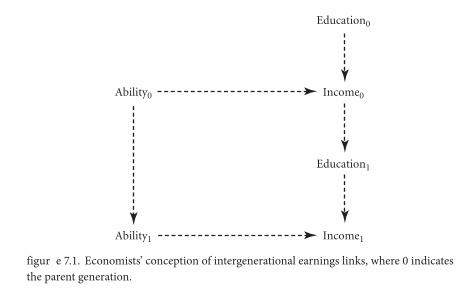
na tur e versus n ur tur e 127
the correlation of underlying abilities. Th is is b ecause education and nurture investments are correlated with underlying abilities.2
Th e economists’ conception seems intuitive and is shared by many people. Diff erences in innate talent are magnifi ed by diff erences in individual families’ income and resources.
Th is picture of mobility mechanisms also implies that the intergenerational correlation of outcomes in t he free-market economy is hig her than is s ocially desirable. Children with the same innate abilities do no t get equal chances in life. Th ose from higher-income families do better. Children of parents of mod-estly lower innate abilities become adults with substantially poorer outcomes because they receive fewer resources from their parents. Assuming that educa-tion and nurture investments by higher-income families are productive, the state should intervene to subsidize such investments in poorer families and promote equality of opportunity.
2 Gary S olon recently formulated a sim ple mo del o f t he contribution of e ach of t hese paths of inheritance that concludes that the intergenerational correlation of earnings, assum-
(γ + τ)ing a constant variance of earnings, will be by = ————, where τ is the parent-child correla- (1 + γτ)tion of abilities independent of investments in children, and γ is the elasticity of earnings with respect to human capital investment. If such investments have no eff ect on income, then γ = 0, parents do not invest, and by = τ, from the biological and cultural correlation. But if γ > 0, by > τ so that investment increases child income (Solon 2013).
Ability0 Income0
Education1
Education0
Ability1 Income1
figur e 7.1. Economists’ conception of intergenerational earnings links, where 0 indicates the parent generation.

na tur e versus n ur tur e 133
from a line of successful and prosperous forebears. His great-grandfather Robert Darwin (1682–1754) produced seven children, all o f whom survived to adult-hood. His grandfather Erasmus (1731–1802) produced fi ft een children (born to two wi ves a nd tw o mistr esses), tw elve o f w hom sur vived t o ad ulthood. H is father, Robert Waring (1766–1848), produced six children, all of whom survived to adulthood.10
In a s ocial environment where all t hese children had t o be privately edu-cated, dowries needed t o be provided for daughters, and estates were divided among children at death, human-capital theory would predict that the heedless fecundity of the English social elites of these years would lead to rapid down-ward social mobility. Th e lower classes of preindustrial society, producing only modestly more than two sur viving children per family on average, would be able to concentrate resources on the care and education of their off spring and see them rise rapidly on the social ladder.
In contrast, by 1880 in England, upper-class men s eem to have produced far fewer children than those of the middle or lower classes. Indeed, from 1880 to 1940, the richest English families seem to have been dying out. Based on the
10 Jenkins (2013) supplies the genealogical information on the Darwin family.
0
2
1
1 2 3 4 5
Wealth decile6 7 8 9 10
3
4
5Su
rviv
ing
child
ren
1500–1780
1780–1879
figur e 7.2. Surviving children per father by wealth at death.

134 ch apter s e ven
rare-surname samples of chapter 5, the upper-class males p roduced, on aver-age, fewer t han two children w ho sur vived to adulthood. At t he middle a nd bottom of society, however, men w ere producing an average of 2.5–3 children who survived to adulthood, in reversal of the pattern observed before 1780. Fig-ure 7.3 shows, by twenty-year periods, the estimated total number of children surviving to adulthood per adult male for two wealth cohorts: initial rich and initial poor or average-wealth rare surnames. Fertility for the richer lineage is consistently less than that of the poorer in the years 1800–1959.
Th is major change in t he relationship between fertility and status can be illustrated again by the Darwin family. Charles Darwin (fi gure 7.4), marrying in 1839, had ten children, though only seven survived childhood. Th es e seven children produced only nine gra ndchildren, an average of only 1.3 per child. (Th is fi gure is un usually low for this era, b ut there was gr eat randomness in individual fertility.) Th e nine grandchildren produced in turn only twenty great-grandchildren, 2.2 p er gra ndchild. Th is fi gure was less t han t he p opulation average for this period. Th e great-grandchildren, born on average in 1918, pro-duced 28 great-great-grandchildren, 1.4 each.11 Th us by the time of the last gen-eration, born around 1918, average family size for this still rather elite group had
11 Jenkins 2013.
0
3
2
1
1880 20001960 1980194019201900
Surv
ivin
g ch
ildre
n pe
r m
an
RichPoor and average
figur e 7.3. Surviving children per adult male by twenty-year period, rich and poor.

na tur e versus n ur tur e 135
fallen to substantially less than replacement fertility. Th e Darwin lineage failed to maintain itself in genetic terms.
Interestingly, with respect to social mobility rates, the twenty-seven adult great-great grandchildren of Charles Darwin, born on average nearly 150 years aft er Darwin, are still a s urprisingly distinguished cohort. Eleven are notable enough to have Wikipedia pages, or the like, such as Times obituaries, devoted to them. Th ey include six uni versity professors, four authors, a pa inter, three medical doctors, a w ell-known conservationist, and a fi lm director (now also an organic farmer).12
But w e s ee no sign s t hat s ocial mob ility ra tes in En gland slo wed as t he upper-class groups produced fewer children. Instead, as c hapter 5 shows, the intergenerational co rrelation o f st atus r emained co nstant f or ed ucation a nd wealth. By implication, human-capital eff ects on social mobility must be mod-est. Status is strongly inherited within families mainly through genetic or cul-tural transmission, or both.
12 It is als o in teresting t hat D arwin’s f ourth-generation des cendants inc luded A drian Maynard Keynes and William Huxley Darwin, showing the intermarriages between the lin-eages of John Maynard Keynes, Aldous Huxley, and the Darwins. Th is illustrates the inter-marriage of the English intellectual elite in these years.
figur e 7.4. Charles Darwin, 1881.

na tur e versus n ur tur e 137
Th e huge size of the Danish wealth data set means that the authors can divide the parents into percentiles and look at the average wealth of children for one hundred sets of parents, measured again as a percentile of the child wealth distri-bution. Other than the top and bottom 3 or 4 percent of parental wealth, the pic-ture has the same linear character as that for height inheritance. One persistence rate, 0.20, des cribes inheritance across the middle 90 p ercent of the distribution (fi gure 7.6).
Th e greatest deviation appears in the bottom 4 percent of parental wealth, where the children are much richer than we would expect. But the parents at the bottom of the distribution in Denmark have negative wealth—that is, debt. Th is suggests not chronic, grinding poverty (no one, aft er all, lends much to the truly poor), but more likely indebtedness to fi nance a business venture or train-ing. Th e fact that this is not truly the bottom of the wealth distribution explains the breakdown of the stable relationship.
Children in t he top 3 percent of the parental-wealth distribution also show slightly greater wealth inheritance. Although this eff ect is statistically signifi cant, it represents only modest deviations from the single persistence rate in r eal terms: the persistence rate implied for the top percentile is 0.24, as opposed to 0.20 for the rest of the distribution. For the second percentile, it is 0.23, and for the third 0.22.
65
71
69
67
63 73716967
Average of parent heights (inches)65
Hei
ght o
f chi
ld (
inch
es)
figur e 7.5. Francis Galton’s observations of biological inheritance of height.

138 ch apter s e ven
Th is result, showing the same intergenerational correlation all acr oss the status distribution, is found also in England. For the period 1858–2012, we can measure social mobility by looking at the representation of surnames among Oxford and Cambridge students, which typically describes the upper 1 percent of the educational distribution. We can also measure social mobility by looking at probate rates: the probated elite was typ ically 15–45 percent of the popula-tion, much closer to median status. Th e estimated mobility rates are the same from these two sources.
Th ere is a t le ast o ne ex ception t o t his r ule o f unif orm p ersistence ra tes across the status distribution. A study by Anders Björklund and others found that in Sweden, although the overall correlation of income across one genera-tion was 0.26, f or the top 0.1 percent of the income distribution, it was much higher, at 0.9.15 However, their study found that this eff ect was caused largely by the exceptionally high levels of wealth among the sons of the very high-income fathers. Th ere was no unusually strong transmission among the top 0.1 percent of educational attainment, high cognitive abilities, or high noncognitive abili-ties. Th us while there may be exceptions to the rule of a co nstant persistence
15 Björklund, Roine, and Waldenström 2012.
�0.6
0.8
0.6
0.4
0.2
0.0
�0.2
�0.4
�3 3210�1
Parent wealth
�2Chi
ld w
ealth
figur e 7.6. Social inheritance of wealth, Denmark, 1997–2012.

indi a 145
Caste affi liations determined centuries ago still strongly predict current educa-tional outcomes.
One factor that might be expected to promote mobility, however, is the res-ervation system. Since Independence, the number of places reserved and the number of groups eligible for reserved places has increased. Up to half of avail-able educational places and government jobs are now reserved.3 If the caste sys-tem trapped many potentially talented people at lower levels of society in t he premodern era, t hen modern reservation policy could be expected to rapidly increase social mobility. Th us, while fi gure 8.1 implies continuing dramatic social inequalities, it is not clear whether we should expect high or low rates of social mobility today, given Indian social policy.
Table 8.1 shows numbers o f ca ndidates in va rious admissio ns ca tegories admitted to the All India Institute of Medical Sciences for the Bachelor of Med-
3 Th e Indian Supreme Court has ruled that no more than half of available positions can be reserved for disadvantaged groups, but some states have higher quotas. Tamil Nadu, for example, has reservations for 69 percent of positions. Th e legality of these quotas is still being litigated.
0Muslim Sikh Hindu,
forwardcastes
Christian
2
Hindu,scheduled
castes
Hindu,other
backwardcastes
4
6
8
10U
niv
ersi
ty g
radu
ates
(%
)
figur e 8.1. University graduation rates by social group, India, 2000.

146 ch apter eight
icine degree in 2012, as well as their rank on the entrance exam. Of the seventy-two candidates admitted, only half w ere admitted solely on the basis o f their admissions exam score. Th e lowest ranking for any student in t he open cate-gory on this exam was 36, compared to 2,007 for the reserved category.
Th ere are surprisingly few formal studies of social mobility in India.4 Th us the two recent international surveys of social mobility discussed in the introduc-tion, one for earnings and the other for education, do not include India.5 How-ever, a recent study estimated the Indian intergeneration income correlation to be 0.58, making social mobility rates in India among the world’s lowest.6
Th e estimated persistence rate for income in India of 0.58, however, is not much higher than those for the United Kingdom (0.5) or the United States (0.47). Th e share of income variance in the next generation attributable to inheritance from parents in I ndia i s s till only (0.58)2, or 0.34. Th is sug gests t hat e ven in India, a n indi vidual’s p osition in t he inco me ra nks is no t p rimarily der ived from inheritance. Th us, by conventional estimates, modern India has become a society of rapid social mobility, where three to four generations might see the elimination of all traces of millennia-old patterns of inequality.
4 Th e large agricultural population makes it diffi cult to classify occupational status. Mo-bility studies based on occupation are thus diffi cult to interpret and to compare with those from more developed economies. See, for example, Nijhawan 1969; Kumar, Heath, and Heath 2004; Hnatkovska, Lahiri, and Paul 2013.
5 Corak 2013; Hertz et al. 2007.6 Hnatkovska, Lahiri, and Paul 2013. Th e researchers actually estimate the income elastic-
ity, which equals the correlation only if the variance of log incomes is constant.
t a bl e 8.1. Admissions to the All India Institute of Medical Sciences, Delhi, by reservation-system category, 2012
Numerical rankCategory Number on admission test
Unreserved 36 1–36Scheduled caste 11 288–1,164Scheduled tribe 5 177–2,007Orthopedic physically handicapped 1 1,201Other backward classes (non-creamy layer) 19 41–116All 72 1–2,007

148 ch apter eight
Th e surnames of Kulin Brahmins are the most overrepresented of all sur-name types among modern Bengali elites. Th ey are more than four times as fre-quent among physicians registered in r ecent decades as in t he general popu-lation. Th ese na mes a re lik ely t o b e fa miliar t o a nyone w ho has met I ndian physicians, professors, or engineers in the United States.
Other sur names ass ociated wi th t he hig h-status B rahmin a nd K ayastha castes in B engal a re als o overrepresented, t hough no t t o t he s ame degree as Kulin Brahmin surnames. Th ese include the surnames Basu/Bose, Datta/Dutta, Ghosh, Kundu, Mitra, and Sen or Sengupta, which were all hig h status in t he nineteenth century. Th ese surnames form the “other elite Hindu” group in fi g-ure 8.2. Basu, Ghosh, and Mitra, for example, are associated with the Kulin Kay-astha (scribe) subcastes, which were regarded as next in st atus aft er Brahmins in premodern Bengal. As with Brahmins, Kulin denotes a superior subcaste.
In contrast, the surnames of the Muslim population are dramatically under-represented among both physicians and judges. Muslims formed a la rge pro-portion of the population in Bengal before Independence and continue to do so in t he co ntemporary st ate o f West B engal. B ecause Muslim a nd H indu fi rst names are also distinctive, the fraction of Muslim physicians in B engal in t he years 1860–2011 is easily estimated.
0
4
3
2
1
5
6R
elat
ive
repr
esen
tati
onDoctors
Judges
PoorestHindu
Scheduledcaste elite
Other eliteHindu
KulinBrahmin
Muslim MixedHindu
figur e 8.2. Relative representation of surname groups among physicians and judges.

150 ch apter eight
sion of social mobility, for these other groups relative representation is shown always with respect to the non-Muslim population only.
Measured by this standard, there has been very little social mobility among Hindu surname groups in Bengal since 1860. Th e Brahmin group of surnames is almost as heavily overrepresented among the non-Muslim population in the period 1980–2011 as it was in 1860–89. Other elite Hindu surnames show a slow rate of decline in st atus. But the relative representation of mixed Hindu sur-names, which are modestly elite, does not change. And the relative representa-tion of poor Hindu surnames of the nineteenth century, those with the highest potential for regression to the mean, also changes little. Th e only group show-ing a marked change in status is the group of surnames associated with sched-uled caste lists for positions in universities and the police. Th is group went from being modestly disadvantaged among non-Muslim groups in 1860 to being one of the most elite surname groups, as measured by their relative representation among physicians now.
Table 8.2 summarizes the persistence rates associated with these surname groups. Th ese ra tes sho w ho w q uickly t he st atus o f t hese gr oups is mo ving toward t he p opulation me an. With a st able variance of st atus across genera-tions, they are also the intergenerational correlation of status. In that case they will be between zero and one. However, these persistence parameters are oft en
8.00
1.00
2.00
4.00
0.02
0.03
0.06
0.13
0.25
0.50
1860 1900 1940 1980
Rel
ativ
e re
pres
enta
tion
Scheduled casteMuslim
Other elite HinduBrahmin
Mixed Hindu
Poor Hindu
figur e 8.3. A summary of social mobility by surname type, 1860–2011.

indi a 151
greater t han o ne, me aning t hat s ome o f t hese gr oups a re di verging f rom t he mean rather than trending toward it. Th e persistence rate for the scheduled caste surname gr oup ca nnot e ven b e calc ulated f or t he p eriod 1950–2011, since i t crosses the mean, moving from below-average status to above-average status.
t he musl im popul at ionCensus reports exist giving the Muslim share of the population in Bengal and West Bengal for each decade from 1871 on. Th us there are good measures of the relative representation among physicians in Bengal from 1860 on. Th e striking feature is the very low representation of Muslims among physicians in all peri-ods. Under B ritish r ule, M uslims exp erienced limi ted u pward mob ility. Th e implied persistence of status was high, with a calculated intergenerational cor-relation of 0.91.
However, from the 1970s until very recently, the Muslim community in West Bengal saw a further decline in representation among physicians, with no implied regression to t he me an. Indeed, st arting wi th t he generation entering practice since Independence in 1947, the implied persistence coeffi cient is 1.2, indicating that the Muslim community has been diverging further from the mean.
Bengal’s system of reserving educational places and employment opportu-nities f or dis advantaged cast es a nd tr ibes exp licitly ex cludes M uslims a nd Christians: only Hindus, Sikhs, and Buddhists are eligible. West Bengal, unlike some other Indian states, has no t yet introduced reserved educational places
t a bl e 8.2. Intergenerational persistence rates (b) for various groups and periods
Pe rcentage of populationSurname (age 20–29), 1860–1947, 1950–2009, 1 860–1947, 1950–2009,group 2010 al l all non-Muslim non-Muslim
Muslim 3 1.1 0.91 1.20 — —Kulin Brahmin 3.4 1.05 1.05 1.03 0.97Other elite Hindu 5.0 0.87 0.85 0.86 0.85Poorest Hindu, 7.0 1.01 0.85 1.02 0.83 pre -1947 Scheduled castes 3.8 — — 0.84 —Mixed Hindu 11.8 1.10 1.70 — —
Average, all 0.99 1.13 0.91 0.88
Persistence rate

4
2
3
1
00 1 2 3 4 5
Rel
ativ
e re
pres
enta
tion
am
ong
polic
e su
bin
spec
tors
, 200
9
PoorHindu
Muslim
Mixed Hindu
Elite Hindu
Scheduledcastes
KulinBrahmin
Relative representation among physicians, 2000–2011
10
8
6
4
2
01860 198019601940192019001880 2000 2020
Rel
ativ
e re
pres
enta
tion
AllNon-Muslim
Independence
figur e 8.4. Relative representation of surnames among physicians and police sergeants.
figur e 8.5. Kulin Brahmin relative representation among Bengali physicians and non-Muslim Bengali physicians, 1860–2011.

156 ch apter eight
t he sch edul ed c a st e e l it e sur na me g r oupTh e p eculiarity o f t he s cheduled cast e sur names iden tifi ed a bove i s th at al-though all of them fi gure prominently in the scheduled caste list, they also fi g-ure signifi cantly in t he list o f B engal p hysicians f rom b efore I ndependence. Indeed, as fi gure 8.6 sho ws, t hese sur names w ere alr eady f ully r epresented among physicians relative to their share in the population in the last generation before Independence. Looking just at the share of these surnames among the non-Muslim population, they were at less than half their expected representa-tion in the period 1860–89 but were converging toward proportional represen-tation, with a persistence rate of 0.84.
Th e success of this surname group under the reservation system has led to these surnames becoming as overrepresented as many higher-caste Hindu sur-names among both physicians and police recruits (see fi gure 8.2). Because they start just below the mean representation in the fi rst generation aft er Indepen-dence, there is no implied regression to the mean for this group. Th ey are defy-ing t he law of s ocial mobility presented in c hapter 6, w hich predicts t hat all groups regress to the mean.
Th is recent overrepresentation of these surnames among physicians, even with r espect t o t he no n-Muslim p opulation o nly, s eems t o b e dr iven b y t he reservation system. In a list o f recent admissions to medical s chools in West
3
2
1
01860 1890 1920 1950 1980 2010
Rel
ativ
e re
pres
enta
tion
am
ong
phys
icia
ns
Scheduled caste / non-MuslimScheduled caste /all
Independence
figur e 8.6. Th e curious history of the scheduled caste surname group.

indi a 159
t a bl e 8.3. Implied persistence of status with and without the reservation system, medical-school admissions, Bengal, 2000–2011
P ercent Implied admitted Relative intergenerational through representation correlation, R elative reservation 2000–2011, 1935–2005, Surname representation, system, no reservation no reservation group 2 000–2011 2010–12 system system
Kulin Brahmin 3.96 0 5.49 1.08Other elite Hindu 2.25 3 3.02 1.07Mixed Hindu 1.70 45 1.30 0.87Scheduled caste 2.90 70 1.20 —Poorest Hindu 0.10 25 0.10 0.77Muslim 0. 12 0 0.17 0.96
8.00
4.00
2.00
1.00
0.03
0.13
0.06
0.25
0.50
1920
Rel
ativ
e re
pres
enta
tion
1950 1980 2010
KulinBrahmin
Scheduledcaste
Other eliteHindu
MixedHindu
PoorestHindu
Muslim
figur e 8.7. Social mobility by surname type without reservation system, 1920–2011.
high-status groups. But it has also served to increase persistence for a large and growing underclass of Muslims and poor Hindus who are ineligible for sched-uled caste status.
It is also not clear whether the system is doing much to increase these over-all slo w ra tes o f s ocial mob ility. A s e videnced b y sur name distr ibutions, t he

indi a 161
detailed study of a mo dest-sized town in B engal in t he late 1960s.16 Another study, looking at marriages in rural villages in Karnataka and Uttar Pradesh for the years 1982–95, found that of 905 marriages in the study, none involved cou-ples who diff ered in their caste status.17 In Hyderabad, among Kayasthas, only 5 percent of marriages were outside the caste even in t he period 1951–75.18 In-formation o n t he degr ee o f endoga my f or ma rriages in B engal in t he 1970s and 1980s, w hich produced the most r ecent crop of physicians, is no t readily available.
One source of information on the likely endogamy rate is the 2010 Kolkata voter roll, which gives surnames, fi rst names, and ages of all voters. Many fi rst names are highly specifi c to the Hindu, Muslim, and Christian/Jewish commu-nities. Table 8.4 sho ws the most co mmon ten fi rst names for women in e ach religious gr oup. Women w ho ma rry in to o ne o f t hese gr oups f rom a nother group will almost always have diff erent fi rst names from women born in within the group. Also, if families with surnames associated with one group are assimi-lated into another group, then, as a r esult of intermarriage and adoption of at least some elements of the culture of the wives, the children again would typi-cally have diff erent fi rst names.
16 Corwin 1977.17 Dalmia and Lawrence 2001.18 Leonard and Weller 1980, tables 1–3.
t a bl e 8.4. Most common female fi rst names among religious groups, Kolkata, 2009
Ot her high-casteKulin Brahmin Hindu Muslim Christian/Jewish
Krishna G eeta/Gita Salma MarySoma Kr ishna Yasmin ElizabethGeeta/Gita So ma Shabana MariaArati Ar ati Asma MargaretSwapna Me era/Mira Sultana Helen(a)Meera/Mira Na mita Anwari AgnesKalpana Kalp ana Shabnam VeronicaRatna A njali Afsana RosemarySumita S wapna Shahnaz DorothyAnjali P ratima Farzana Teresa

162 ch apter eight
As t able 8.5 shows, t he p ercentage of women in t he Kulin Brahmin sur-name group with non-Hindu fi rst names is extremely small. Because Muslims constitute nearly a q uarter of the Kolkata population, this implies that inter-marriage rates between Kulin Brahmin men and women of Muslim origin are extremely low, on the order of 0.1 percent. A similar result holds for other high-caste Hindu surnames.
More women with Muslim surnames have Hindu fi rst names: 0.9 percent. But given the near-total absence of any sign of Muslim women’s marriage into high-caste Hindu groups, if these fi ndings are indicative of marriage alliances, they are likely with lower-caste Hindus.
Intermarriage b etween Chr istians a nd hig h-caste H indus a ppears t o b e substantially more common. Christian surnames account for a very small share of the surname stock in Kolkata, about 0.3 percent, and are mainly Portuguese in origin. Given this small Christian population, the small share of women with high-caste Hindu surnames who have Christian fi rst names is nevertheless sug-gestive of signifi cant intermarriage.
An alternative explanation for these female Christian fi rst names may be that high-caste Hindu girls are given Christian fi rst names at birth. Th e pos-sibility of signifi cant intermarriage between Christians and Hindus is, ho w-ever, supported by the fact that just over 30 percent of women with Christian surnames have fi rst names that are Hindu. Also, almost 12 percent of women with Chr istian sur names ha ve a co mbination o f Chr istian a nd H indu fi rst names.
Th e fi rst-name a nd sur name e vidence sug gests almost no in termarriage between the largely poor Muslim community and either Hindus or Christians.
t a bl e 8.5. Female fi rst-name origins by surname group
Incidence in surname group (%)
Other high-casteFirst-name type Kulin Brahmin Hindu M uslim Christian
Hindu 99 .6 99.3 0.9 30.2Muslim 0. 1 0.1 98.9 0.4Christian 0 .3 0.6 0.2 57.4Hindu and Christian 0.0 0.0 0.0 11.9

indi a 165
to reserved places in medical schools is heavily underrepresented among Ben-gali physicians working in the United States. Th eir representation in the United States is only a quarter of that in Bengal. Th e mixed Hindu surname group, of whom an estimated 45 percent were admitted to reserved places, show up in the United States at about 40 p ercent less than the rate expected from their repre-sentation in Bengal.
Th ere could be many explanations of these fi ndings. But one possibility is that p hysicians admi tted t o I ndian medical s chools t hrough t he r eservation system fi nd it harder to meet the onerous requirements to practice medicine in the United States: passing the U.S. Medical Licensing Examination and com-pleting the required residencies. Th ough the reservation changes the measured social status of these individuals, it does much less t o change the underlying social competence of these families. If the reservation system were ended, the measured social status of these groups would soon also decline substantially. Another possibility, however, is t hat groups that benefi t f rom the reservation system ha ve f ewer o f t he fa mily r esources needed t o r elocate t o t he United States and practice medicine there. But the observed patterns contain nothing that clearly contradicts the biological explanation.
20
12
16
8
4
00 5 10 15 20
Un
ited
Sta
tes
(%)
Poorest Hindu
MuslimChristian
Mixed Hindu
OtherHindu elite
Scheduledcastes
Brahmin
West Bengal (%)
figur e 8.8. Surname group shares among Bengali physicians in West Bengal versus in the United States.

chin a and t aiw an 169
Red Guards and in defi ance of them. All acr oss the countryside, alleged class enemies were being confronted, abused, and killed (fi gure 9.1). Th e total death toll f rom the chaos of the Cultural Revolution is unkno wn but has b een esti-mated to be as high as ten million.
Institutions o f hig her ed ucation eff ectively c losed b etween 1966 a nd t he early 1970s. Even aft er this, large numbers of urban students were sent out to labor in the countryside, denied the opportunity for higher education. It is esti-mated that as ma ny as eig hteen million people were forced to relocate to the countryside in these years. Admission to universities in the years 1970–76 was largely det ermined b y p olitical q ualifi cation a nd co nnections: o nly st udents without the taint of bourgeois background were admitted. In 1977 the National
figur e 9.1. Administrator of the Heilongjiang Daily denounced by the newspaper staff for following the capitalist line, 1966.

chin a and t aiw an 171
However, i t is p ossible t o iden tify t hirteen r elatively ra re sur names t hat appear with unusually high frequency among those who attained the highest qualifi cation under the Qing exam system, that of jinshi (进士). A complete list has been published of all the Qing jinshi. Indeed, in the front courtyard of the Confucius Temple in B eijing a re hundreds o f la rge st one t ablets b earing t he names o f t he mo re t han fi ft y thousand jinshi o f t he Yuan, M ing, a nd Qin g dynasties. Th ese thirteen elite surnames were identifi ed as those that showed a relative r epresentation a mong Qin g jinshi between 1820 a nd t he end o f t he imperial exam era in 1905 that was at least four times that of the big three sur-names.9 Th ough relatively ra re by Chines e st andards, t he t hirteen eli te Qin g surnames are held by nearly eight hundred thousand people today.10 So there is plenty of evidence by which to judge the current status of these surnames.
Th e imperial examinations were the meritocratic path to high-level posi-tions in the bureaucracy. Th e gains from various levels of achievement on these exams were so great that to limit cheating and nepotism, they were held under strict supervision, with the candidates isolated in individual cells for the two to three days of the exam (see fi gure 9.2). Individual examinations were numbered, and candidates’ answers were copied out by clerks so that the graders could not recognize candidates by their calligraphy. Candidates spent years studying to attempt the various levels of the exams. Th e gains were not just the emoluments
9 It is assumed that the relative frequency of surnames was the same in the period 1645–1905 as in 2010.
10 Th ese surnames represent, however, only 0.055 percent of the modern population.
figur e 9.2. Imperial examination hall with 7,500 cells, Guangdong, 1873.

chin a and t aiw an 173
education institutions between 1966 and 76.) Th ese three groups are observed roughly seventy-fi ve years, or 2.5 generations, aft er the high Nationalist offi cials of 1912–49. Assuming that the Nationalist offi cials were a similarly exclusive elite, the intergenerational correlation of status for these surname groups between the Republican era and 2006 is 0.9 for professors, 0.8 for company board chairs, and 0.74 for central government offi cials.
Assuming that the jinshi elite of 1820–1905 and the Nationalist offi cials of 1912–49 were also comparably elite groups, it is als o possible to calculate the mobility rate between these two eras.11 Th e decline of the relative representation of the thirteen Qing elite surnames among the Nationalist offi cials implies an intergenerational correlation of status of 0.8.
Th ese r esults a re su pported b y da ta o n st udent admissio ns t o Tsinghua University from 2003 to 2011. As one of the top ten universities in China, Tsin-ghua again represents an elite at the pinnacle of the education distribution. Th e relative representation of the thirteen Qing elite surnames, even relative to the three regional surnames, was still 1.62. Since these students, entering university
11 Based on the numbers listed per year, there were more jinshi than high Nationalist offi cials.
0
4
3
2
1
5
6
7
8
9
10R
elat
ive
repr
esen
tati
onQing elite/big three surnames
Qing elite/Gu-Shen-Qian
Jinshi ,1820–1905
Professors,2012
Corporateboard chairs,
2006
Nationalistofficials,1912–49
Governmentofficials,
2010
figur e 9.3. Relative representation of Qing elite surnames among modern Chinese elites.

176 ch apter nine
Again, unusual Qing-era success on the imperial exams is used to identify the early elite surname–place of origin combinations in these two regions. Th e records used in t his case are the far more numerous ones of the juren, those who succeeded at the provincial level of the imperial examinations. Surname-location combinations that occurred at fi ve times or more of the expected fre-quency among juren in each location from 1871 to 1905 were classifi ed as con-stituting local surname elites.
To trace t he status of these groups into the present, we need t o know the family place of origin for members of various later elites. Th is information is available for the Republican era b ecause it was inc luded in uni versity rosters and alumni records, which provide data for eleven thousand students.
Under co mmunism, suc h f orms o f iden tifi cation b ecame less co mmon. Th e Communists, aft er all, wanted to remake society, not perpetuate the ancient lineage of successful families. But fortunately, two sources from the Commu-nist era s till reported family places of origin at the county level. For modern Zhejiang, the Zhejiang Provincial Archive lists no table Zhejiang people born between 1930 and 1990 and includes the family place of origin. Th is list covers a
North ZhejiangSouth Jiangsu
figur e 9.4. Th e areas of the lower Yangzi used in the surname–place of origin mobility estimates.

chin a and t aiw an 177
spectrum of occupations, such as entrepreneurs, artists, professors, and offi cials; of these, only those with a university degree were counted as elite. Th e notable people list also includes, conveniently, people who migrated from the region.
Data on later elites is obtained for South Jiangsu from the Nanjing Univer-sity archive, which records students by name, place of origin, and year of grad-uation f or t he y ears 1952–2010. Th is in stitution ra nks t hird a mong Chines e universities, and two-fi ft hs of its students are from Jiangsu. To enroll, students must rank among the top 3 to 5 percent of those taking the National College Entrance Examination (gaokao [高考]). Since less than half of each cohort typi-cally took this exam in the Communist era, Nanjing students represent the top 0.6 to 2.5 percent of the South Jiangsu distribution of scholastic achievement.
Comparing the relative representation of the 1871–1905 exam elite in tw o subsequent Republican elites—students and offi cials—in the years 1912–49 gives an estimate of persistence rates for the Republican era of 0.78–0.81, consistent with estimates in many other societies (see table 9.1).
Th e implied social mobility in N orth Zhejiang for the Communist era is not signifi cantly higher: the persistence rate is still 0.74. Th is mobility estimate is partly based, however, on the achievements of people born in Zhejiang who emigrated to Taiwan, Hong Kong, or the United States but were still included on the list of notable people.
In S outh J iangsu, bas ed o n t he N anjing st udent r ecords f or 1952–2010, social mobility rates for the Communist era were higher than before. But there was still a s trong connection between surname–place of origin combinations overrepresented in 1952 and those overrepresented in 2010. (A gain, given the modest s ample sizes, t here ma y b e co nsiderable s ampling er ror underl ying these estimates.)
Overall, although these local estimates do suggest faster social mobility in the Communist era, they also imply a remarkable persistence of status in a soci-
ta bl e 9.1. Persistence rates for the lower Yangzi, 1871–2010
Period Surname groups North Zhejiang South Jiangsu
1871–1949 Juren, University students 0.78 0.81 1930–90 Notable people 0.74 —1952–2010 Nanjing University students — 0.66

chin a and t aiw an 179
are low compared to those seen in t he other surname studies. Th e y certainly suggest, ironically, that social mobility aft er 1949 was faster in class-ridden Tai-wan than in the class-free society Mao built.
However, aft er the 1950s t here was signifi cant migration f rom Taiwan to the United States and Canada, mainly by the more-educated mainlander popu-lation. I n t he U nited S tates, t hese immigra nts a nd t heir des cendants ha ve among the highest university graduation rates of any community. Such migrants in the United States and Canada now number 0.7 million, equivalent to 3 per-cent of the population of Taiwan. Th e subtraction of this mainlander elite from the p opulation o f Taiwan b y emigra tion incr eased estima ted s ocial mob ility rates within Taiwan. Th ere are consequently fewer mainlanders at National Tai-wan University or working as medical do ctors and business leaders. Th er e are correspondingly more native Taiwanese in these positions who are descended from families that were lower class in 1949.
Th e information does not exist to allow Hao to estimate what the true per-sistence rates would have been absent this migration. He cannot observe exactly how selective the migration was or how concentrated among mainlanders. We can be confi dent, however, that the mobility rates reported in table 9.2 overstate true rates of social mobility.
Yu Hao estimates counterfactually that this eff ect could have reduced mea-sured p ersistence rates for educational st atus by as m uch as 0.06. 16 Table 9.2 shows the estimated persistence rates with this upward adjustment. Th e average measured p ersistence ra te is 0.66, w hich is no w no t fa r b elow t he estimates found for other countries. And, as noted, the eff ects of emigration are hard to estimate.
16 Hao 2013, chapter 3.
t a bl e 9.2. Persistence rates for Taiwan, 1949–2012
P ersistence rate
Adjusted for emigrationGroup Unadjusted of mainlander elite
National Taiwan University students 0.55–0.66 0.61–0.72Medical doctors 0.53–0.65 0.59–0.71Business leaders 0.58–0.62 0.64–0.68

japan and k o r ea 183
on selection for higher-level institutions through competitive examination. Th e samurai thus soon lost all c lass privileges in t he rapidly modernizing Japanese economy.
As pa rt o f i ts mo dernization p rogram, t he M eiji g overnment s ought t o enforce a sha red cultural identity and set of cultural practices. Th e reformed educational system promoted a standard form of spoken Japanese nationwide. Th e government was a ided in t his eff ort by t he relative homogeneity of lan-guage, culture, and even physiognomy among most Japanese.
Aft er the Meiji restoration, the new leadership, as part of its Westernization program, merged the kuge, the ancient court nobility of Kyoto, with the daimyo, the feudal lords, into an expanded aristocratic class. Th e resulting kazoku peer-age initially consisted of just 427 families. However, the Meiji government ex-panded the hereditary peerage by adding to its ranks persons who had made distinguished contributions to the nation. As table 10.1 shows, the total member-ship grew most rapidly between 1884 and 1907. Th us the kazoku families repre-sented an elite of wealth and position in J apan that dates mainly from before 1907, though new families were being added even aft er 1928.
Th e kazoku had a n umber of privileges in addi tion to any private wealth that t hey r etained f rom p re-Meiji times. S ome r eceived her editary p ensions from the state. Th e titles and pensions passed by inheritance to the eldest son. Only the holder of a title was considered part of the kazoku: other children had no special status. Th e kazoku elected representatives from their ranks to serve in the House of Peers.
figur e 10.1. Samurai of the Satsuma clan during the Boshin War period (1868–69).

184 ch apter ten
Th e ne w co nstitution o f 1947 eliminated t he im perial eli te: t he kazoku was abolished, and these families were all rendered ordinary citizens. Th us for the last two generations Japan has been a society of exceptional social homo-geneity. Visible racial a nd et hnic minorities are f ew: t hey inc lude t he Ainu, some islanders, and the descendants of Korean immigrants from the colonial era. S ocial p olicy has e ven ma naged t o r ender invisible t he burakumin, th e descendants of the outcast communities of the feudal era w hose occupations rendered them defi led and impure. Religious minorities, such as Chr istians, have remained a small sha re of the population. And in g eneral the Japanese now register in the World Values Survey as the most secular population in the world.1
Sociological studies support the idea that Japan is a n intergenerationally mobile society. One study, for example, looked at the occupations of three cross sections of fathers and sons in 1965, 1975, and 1985.2 If we assign an income level to each of these occupations, we can translate these results into the intergenera-tional earnings correlation. Using average earnings by occupation gives an im-plied persistence rate of 0.3 in all these cohorts.3 A more recent study of inter-generational income mobility found implied intergenerational correlations of 0.3–0.46.4 Th us, on conventional measures, Japan has plenty of intergenerational mobility.
1 Inglehart and Welzel 2010, 554.2 Jones, Kojima, and Marks 1994.3 Clark and Ishii 2013.4 Ueda 2009.
t a bl e 10.1. Number and rank of kazoku families, 1884–1946
Year P rince/marquess/count Viscount Baron Total
1884 111 324 74 5091887 1 17 355 93 5651899 1 44 363 221 7181907 1 51 376 376 9031916 1 55 380 398 9331928 1 66 379 409 9541946 — — — 1,011

japan and k o r ea 185
soci a l mobil it y a mong t he sa mur a i in t he e a r l y meiji er aAs the class of bureaucrats and offi cials, the former samurai began the Meiji era with considerable advantages. Th ese were refl ected in admissio ns to the newly formed universities and technical colleges, in which the descendants of the sam-urai c lass w ere he avily o verrepresented. Table 10.2 sho ws t he p ercentages o f samurai and commoners in the major higher-education institutions in 1890 and 1900. Since the descendants of the samurai constituted 5.3 percent of the popula-tion, in 1890 the samurai were graduating at twelve times the expected rate from imperial universities, and commoners at less than half the expected rate.5
Th e proportion of commoners in the universities rose quickly, however. By 1900, s amurai were graduating at only nine times t he expected rate. However, because the samurai were so heavily overrepresented initially, the rate of decline in their advantage is still slow once we calculate the implied persistence rate.
Table 10.3 shows the implied relative representation of the samurai in t he universities and the implied intergenerational correlation of educational status. Th is analysis assumes that university students represented the top 1 percent of the status distribution and that by 1890 the samurai had t he same variance of underlying s ocial st atus as t he g eneral p opulation. Th e im plied in tergenera-tional correlation is high, 0.66–0.72. A wider estima te, based on a more com-prehensive set of higher-education programs, suggests an average persistence rate of 0.73 for this period.6 Th us even though the raw data of table 10.2 might appear to suggest high rates of social mobility, it actually implies slow mobility rates during the Meiji era.
Th is intergenerational correlation in status is calculated assuming that the samurai sha re o f t he uni versity-aged p opulation r emained co nstant b etween 1890 and 1900. Th ere is reason to believe that, if anything, their population share was declining. For example, the source that gives samurai and commoner pop-
5 Amano 1990, 192.6 Clark and Ishii 2013.
t a bl e 10.2. Class status of university graduates, 1890–1900 (%)
18 90 1900
Samurai C ommoners Samurai C ommoners
Imperial universities 63 37 51 49Other universities 62 38 48 42

186 ch apter ten
ulations in 1881 estimates an average family size for samurai of 4.54, compared to 4.78 for commoners.7 Any decline in the share of samurai in the young popu-lation between 1890 and 1900 w ould imply a smaller dec line in relative repre-sentation of samurai at universities and professional schools and hence an even higher persistence rate.
Harry H arootunian gi ves t he sha re o f cen tral a nd lo cal g overnment employees in 1872 to 1882 who were of samurai origin.8 Th es e fi ndings are sum-marized in t able 10.4. Th e share of s amurai among government offi cials also greatly exceeded their share in the general population in 1872. But as with grad-uates of the universities, this share began immediately to decline. Again, how-ever, the rate of decline was consistent, with a high rate of persistence of 0.72. (Th is persistence rate again is calculated assuming that the samurai population share was constant over time.) So despite the many social and economic changes occurring in J apan in t he Meiji period, the rate of downward mobility of the former samurai is once again the standard rate. Th is was another social revolu-tion that had surprisingly little bite on the social elite.
7 Sonoda 1990, 103.8 Harootunian 1959.
t a bl e 10.3. Implied persistence rates for the samurai, 1890–1900
Implied 1890 18 95 1900 p ersistence rate
Imperial universities 11.9 11.1 9.6 0.72Higher schools 11.6 11.2 9.0 0.66
Relative representation
t a bl e 10.4. Percentage of samurai government offi cials and persistence rates, 1872–82
Year Central government Local government
1872 7 8 701876 7 8 —1882 6 1 58
Implied persistence rate 0.71 0.72

japan and k o r ea 189
ingly, the samurai surnames, despite their being selected from a g enealogy of 1812, are still much more heavily overrepresented in four of the fi ve high-status groups in the modern era than are the kazoku surnames.
Th e expectation is that the rarer these surnames are today, the more likely that the holders are actually samurai or kazoku descendants. Th us the rarer the
t a bl e 10.5. Th e rare surname samples
Kazoku Samurai
Im plied Implied nu mber of number ofEstimated number Number of people with Number of people withof surname holders surnames na mes su rnames names
0–99 5 9 1,658 68 1,638100–199 1 5 1,890 18 2,450200–399 1 9 5,940 19 5,714400–999 3 3 24,098 69 48,4801,000–1,240 7 7,757 15 16,514
All 1 32 41,343 189 74,797
0
4
3
2
1
5
6
7
Rel
ativ
e re
pres
enta
tion
Samurai
Kazoku
Medicalresearchers
Managers ProfessorsAttorneys Scholarlyauthors
figur e 10.2. Relative representation of rare surnames among high-status groups, Japan, 1989–2012.
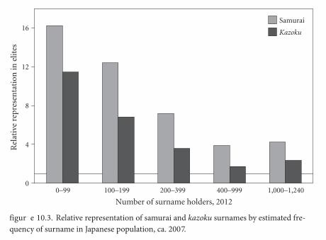
190 ch apter ten
surnames, the greater their predicted overrepresentation among elites. Figure 10.3 shows relative representation controlling for the frequency of the surnames. Sev-eral things stand out. First, the rarer the surname, the higher indeed i ts relative representation. Th e rarest surnames are 12–16 times overrepresented, whereas the most common are only 2–4 times overrepresented. Some of this eff ect may, how-ever, be a statistical artifact. Since these surname frequencies are based on only a sample (though a very large one) of family surnames in Japan, they give an imper-fect measure of the stock of each surname in t he population at large. Th us the surnames assigned to the rarest groups tend to be those whose true frequency in the population is greater. Experience elsewhere suggests that the true frequency of these rarest surnames is at least a quarter greater than reported.
But t he overrepresentation of t he rarest sur names is s o great t hat e ven if their true frequencies were double the reported fi gure, they would still be greatly overrepresented. Th is supports the idea that the rarer the kazoku or samurai sur-names now, the more likely it is t hat modern bearers of the name are descen-dants of kazoku or samurai forebears.
Second, as b efore, samurai surnames, even controlling for frequency, are now more overrepresented among elites than kazoku surnames. If samurai de-scendants never intermarried with descendants of commoners, then, assuming
figur e 10.3. Relative representation of samurai and kazoku surnames by estimated fre-quency of surname in Japanese population, ca. 2007.
0
8
4
12
16
Rel
ativ
e re
pres
enta
tion
in e
lites
Samurai
Kazoku
0–99 200–399 400–999100–199 1,000–1,240
Number of surname holders, 2012

japan and k o r ea 191
the same fertility, their descendants would now constitute 5 percent of the pop-ulation. But fi gure 10.3 suggests that samurai descendants may be as m uch as ten times overrepresented among modern Japanese elites. Th at rate implies that half the modern elites are descended from the samurai. Intermarriage would greatly expa nd t he sha re o f t he mo dern p opulation o f s amurai des cent. B ut if t he s amurai a re r eally t en times o verrepresented in mo dern eli tes, in ter-marriage must have been limited, so that their descendants constitute no more than 10 percent of the modern population.
Tracking the most common surnames provides confi rmation that the samu-rai and kazoku descendants are still heavily overrepresented among modern Jap-anese elites (fi gure 10.4). Most commoners acquired surnames only aft er 1868, when the government required all families to adopt surnames to aid military con-scription, t axation, and p ostal delivery. Many previously hig h-status sur names were adopted by commoners. Th us the name Fujiwara, originally the name of a powerful and distinguished medieval family, is now held by more than three hun-dred thousand Japanese. It is clear that any very common surname in Japan must have been held disp roportionately by commoners in t he Meiji era. Th us, if w e look at the status of the most common surnames, we can determine the relative status of the descendants of the commoners of 1868 in modern Japan.
figur e 10.4. From samurai to salarymen.

192 ch apter ten
Taking the fi ft y most common surnames in Japan, which together account for a q uarter o f t he p opulation, w e fi nd t hat t heir r elative r epresentation among elites in Japan is always less than one. Typically these surnames occur at only 85 percent of the rate expected from their population shares (see fi gure 10.5). Interestingly, t hey a re eq ually under represented a mong p hysicians in Japan and among physicians trained in J apan who are now practicing in t he United States.
soci a l mobil it y r at es, 1900 –2012To calculate the relative representation of kazoku and samurai surnames among elites as far back as 1900 r equires knowing the share of these surnames in t he general population in earlier generations. Th ere is some evidence of lower fer-tility among elites, which would imply smaller elite-surname population shares earlier. In the years 1940–67, for example, marriages involving highly educated husbands or wives produced one-fi ft h fewer births than those of couples with lower educational attainment.17 But the prevalence of adult male adoption among the elite would create a co untervailing tendency for elite-surname population shares to increase, if s ome of t he adoptees originally had a verage-status sur-
17 Hashimoto 1974, S184.
figur e 10.5. Relative representation of common surnames among elites, Japan, 1980–2012.
0.0
0.6
0.4
0.2
0.8
1.0R
elat
ive
repr
esen
tati
on
Medicalresearchers,
Japan
Attorneys ManagersPhysicians,Japanese in
United States

japan and k o r ea 193
names. Absent better data, it is assumed that the population share of these sur-names was the same in 1900 as in 200 7.
Google S cholar gives measures of the number of publications associated with samurai, kazoku, and common surnames for the period 1900–2012.18 To calculate the relative representation of these surnames among publications by Japanese authors requires, however, that the total stock of such publications be estimated for every decade. Th is is done by measuring publications by authors holding the ten most common Japanese names in each decade.19
Figure 10.6 p lots t he r elative r epresentation o f s amurai a nd kazoku ra re surnames among authors of scholarly publications by decade from 1900. B oth the s amurai a nd kazoku sur names a re he avily o verrepresented in t he ini tial decades, wi th p ublication ra tes o f ele ven a nd tw enty-one times t hose o f t he average person in Japan, respectively. Th at relative representation declines over time, but is still more than four for both groups from 1990 to 2012. Indeed, for
18 Clark and Ishii (2013) detail some complications that arise in performing this exercise.19 Th is stock of all publications is adjusted upward by 13 percent to allow for the expected
underrepresentation of common surnames among elite groups such as authors, as seen in fi g-ure 10.5.
2
32
16
8
4
11900 19401920 1960 1980 2000
Rel
ativ
e re
pres
enta
tion
KazokuSamuraiCorrelation 0.88Correlation 0.71
figur e 10.6. Relative representation of kazoku and samurai surnames among authors of scholarly publications, 1900–2012.

194 ch apter ten
both groups, there is a n increase in r elative representation in t he years 2000 and later.
Th e implied intergenerational correlation of publication rates, assuming a standard thirty-year generation, is 0.71 for the kazoku and 0.88 for the samurai. Th ere is no sign o f a ny incr ease in mob ility ra tes a ft er t he r eforms o f 1947. Again, adult male adoption may bias these estimates up by as much as .06. But even allowing for this, social mobility rates are clearly just as low in Japan as in the other countries studied, and they are just as low aft er 1900 as t hey were in the early Meiji period.
Th e magnitude and pattern of these results for authors is confi rmed by the representation of these surnames among medical researchers. Listings are avail-able of medical r esearchers in J apan for 1965–66 and 1989–90, a tw enty-fi ve-year interval. Table 10.6 sho ws t he relative representation of t he kazoku and samurai rare surnames among medical researchers in each year. Th e names are again distinctly overrepresented. In the bottom row of the table are the implied persistence rates, adjusted to a t hirty-year generation. Th e values are slightly lower than for the publications, at 0.6 3 for kazoku and 0.8 2 for samurai sur-names. But this diff erence could be due to chance. Because of the small popula-tions bearing these rare surnames (41,000 and 75,000 respectively circa 1990), the number of observed medical researchers in each period is small.
Another estimate of social mobility in Japan comes from the 2012 American Medical Association directory. Th is lists more than a thousand Japanese-trained physicians practicing in the United States, a fi ft h of whom hold one of the fi ft y most common Japanese surnames. Th e AMA data also give the date of gradua-tion of e ach registrant. Th e Japanese physicians can t hus b e divided into two generations, t hose graduating b etween 1950 and 1979 and t hose graduating
t a bl e 10.6. Relative representation of samurai and kazoku among medical researchers, 1965–89
Year S amurai Kazoku
Observed 1965–66 30 13Observed 1989–90 70 23
1965–66 5 .99 4.951989–90 4 .69 2.94
Implied persistence rate 0.84 0.64

200 ch apter ele ven
the same proportional movements in inco me toward the mean as a re seen in Sweden, where the rungs of the income ladder are closer together. If the rungs on the income ladder are farther apart in the United States or Chile, the upward steps t hat a re p ossible t hrough o ccupational mob ility a re co rrespondingly greater. So the distance between the analogical ladder r ungs explain nothing about rates of social mobility.
In chapter 6 i t was a rgued that the inequality-immobility association is an illusion created by the fact that common measures of social status, such as income, indicate only with some degree of error the true underlying status of families. I n s ocieties lik e S weden, w here ra nges o f inco me a nd w ealth a re compressed, t hese me asures a re pa rticularly p oor indica tors o f underl ying social status. Consequently, these societies seem to have rapid rates of social mobility.
In co ntrast, in a s ociety o f gr eat inco me a nd w ealth ineq uality suc h as Chile, these factors are much better indicators of the true social status of fami-lies: inco me mob ility co mes c loser t o me asuring t he tr ue underl ying ra te o f social mob ility. Th is c hapter investigates w hether s ocial mob ility ra tes in a n inegalitarian society such as Chile truly are lower than in egalitarian Sweden.
figur e 11.1. Shantytown, Valparaiso, Chile.

202 ch apter ele ven
there is good information from the electoral census not just on implied earn-ings, but also on more general implied living conditions.
Underclass and Elite Surname Groups
As in earlier chapters, social mobility in Chile is estima ted by identifying sur-names that had high or low status before 1920 and then measuring how quickly the average status of these surnames regresses to the mean using the informa-tion from the electoral register.
One general feature of Chile’s population is an inverse correlation between social class and degree of indigenous ancestry. Studies suggest that for the upper class, 73–91 percent of their genetics is C aucasian, for the middle c lass 68–70 percent, and for the lower class 41–48 percent.4 So the Mapuche, the major in-digenous population of Chile, would be expected to be at the lowest rung of the social ladder.
4 Cruz-Coke and Moreno 1994, table 2.
figur e 11.2. Salaries by community, Human Development Index grouping.
400
200
1,200
1,000
800
600
00 1,000
Average community wage (thousands of pesos)
500 1,500 2,000 2,500
Ave
rage
occ
upa
tion
al w
age
(th
ousa
nds
of p
esos
)
0.5–0.6
0.6–0.7
0.7–0.8
0.8–0.9
0.9–1.0

206 ch apter ele ven
Table 11.1 summarizes the numbers of people from each of these surname groups in the 2004 census who were born in the periods 1920–49 and 1950–79. Th e ratio of the numbers born in the later period and the earlier reveals the rel-ative social status of these groups. For the country as a w hole, the ratio is 2.3. For the Mapuche, the lowest-status group, this ratio is higher, at 2.47. Th e diff er-ence refl ects a combination of likely higher fertility among poorer groups and lower longevity in the older age cohort.
Confi rmation that the ratio is closely linked to status comes from the sur-names of the 1853 landowners. Ranking these by in increasing order by value of their land, the ratios are 2.26, 2.10, 1.91, and 1.89. Th us 150 years later, in 200 4, the status of landowners in 1853 continues to infl uence outcomes, suggesting that there is considerable intergenerational persistence in Chile.
Table 11.2 shows average occupational income by surname group relative to the average for all persons for those born in the periods 1920–49 and 1950–79. Also shown is the implied intergenerational correlation of average income. Th e individual estimates vary from 0.70 to 0.95, with an average of 0.84. Estimated
t a bl e 11.1. Surname samples in 2004 Chilean electoral register
Ratio (1950–79/ Group N otes 1920–49 1950–79 19 20–49)
Encomenderos E arly elite 839 1,557 1.86Mapuche I ndigenous 7,036 17,389 2.47Basque E arly elite 8,755 17,841 2.04French 1 920 elite 1,402 2,494 1.78German 1 920 elite 2,452 4,337 1.77Italians 1920 elite 1,132 1, 981 1.75Landowners 1853, small 15,988 36,070 2.26 1 853, medium 824 1,731 2.10 1 853, large 1,874 3,580 1.91 1853, very large 857 1,621 1.89 1 920, large 1,680 3,069 1.83Rich, nineteenth century 1,058 2,012 1.90
Number in birth cohort

chile 207
t a bl e 11.2. Intergenerational correlation of occupational and locational income by surname group from 2004 electoral register
Implied Implied correlation, correlation, occupational locationalGroup 1920–49 19 50–79 in come income
Encomenderos 1. 54 1.45 0.76 0.83Mapuche 0. 68 0.75 0.79 0.63Basque 1. 35 1.27 0.75 0.79French 1. 57 1.51 0.88 1.01German 1. 63 1.56 0.93 0.86Italians 1. 67 1.53 0.85 0.89Landowners 1 853, small 1.01 1.01 — — 1 853, medium 1.41 1.27 0.70 0.85 1 853, large 1.59 1.53 0.92 0.82 1853, extra large 1.74 1.71 0.95 0.81 1 920, large 1.79 1.73 0.92 0.81Rich, nineteenth century 1.61 1.54 0.90 0.86
Average — — 0.84 0.83
Occupationalincome relative to
birth-cohort average
correlations using locational estimates of average income are shown in the last column. Th e individual estimates of persistence vary here, but the average is very close to that for occupational income, at 0.83.
As in the other countries, the social mobility rates estimated here are much slower than those estimated by conventional methods. Núñez and Miranda, for example, derive estimates of only 0.52–0.67 for income and educational persis-tence using conventional methods.16
Th e estimates of the intergenerational correlation for the Mapuche, the one poor group in the table, are lower in each case than the average: 0.79 for occu-pational income and 0.63 for locational income. Th ese results may refl ect higher
16 Núñez and Miranda 2007. Th ese are high for conventional estimates compared to those for Nordic countries, or even Canada, the United Kingdom, and the United States.

chile 209
Mobility by Decade
Above, mobility is measured by generation. But it is also interesting to consider mobility b y decade , e ven t hough wi th t his a pproach ra ndom fl uctuations appear because of the smaller amounts of data. Th is approach is of interest for Chile because of its relatively short-term but dramatic social disruptions in the later twentieth century. Th e years 1964–73, under the presidencies of Eduardo Frei and Salvador Allende, saw signifi cant attempts to improve the educational outcomes f or t he p oorer s ections o f Chile an s ociety. Th at s ocial exp eriment came to a calamitous end with Augusto Pinochet’s coup d’état of 1973 (fi gure 11.3) and the ensuing years of repression under military rule. During Pinochet’s dic-tatorship (1973–1990), there was reduced expenditure on public education and programs targeted at the poor and an expansion of the private sector in higher education. If public support had any eff ects on social mobility, then we would expect that the people born in the decade 1950–59, many of whom enjoyed the benefi ts of t he Frei and Allende s ocial programs as t hey attended s econdary school and college, would experience enhanced mobility. In contrast, the people born in the decade 1970–79, most of whom were educated in the Pinochet years, should experience more restricted mobility.
figur e 11.3. Th e assault on the presidential palace during the 1973 Chilean coup d’état.

210 ch apter ele ven
Figure 11.4 shows o ccupational inco mes b y decade f or a s et o f sur name groups f rom t he colonial era, inc luding t he encomenderos and t he Mapuche. Th e incomes are shown essentially as their variation above and below the mean occupational income for people of that decade.17 Th e scaling of the fi gure means that social mobility rates are portrayed by the slope of the line. It is evident that the political regimes of 1964–73 and 1973–90 had li ttle perceptible impact on social mob ility ra tes. Th e 1950–59 b irth co hort did no t s ee a ny syst ematic increase of mobility rates, despite the enhancement of educational opportuni-ties for the poor under F rei and Allende. Th e 1970–79 cohort did no t see any systematic decline in social mobility. Th ere was indeed an apparent increase in occupational status for the encomendero surnames. But that is bas ed on small numbers and may be subject to sampling error.
Figure 11.5 shows the variation in o ccupational incomes by decade for other elite-surname groups: French, German, Italian, and the rare surnames of medium and large landowners in 1853. Again there is no sign o f any systematic enhanced mobility for the 1950–59 birth cohort. Th ere is a modest sign, however, of a decline in downward occupational mobility for those educated in the Pinochet years.
17 Technically the fi gure shows average log inco me for each surname group minus the Chilean average log income.
�0.2
0.6
0.4
0.2
0.0
�0.41920 19401930 1950 1960 1970 1980
Ear
nin
gs d
iffe
ren
ce fr
om a
vera
ge
Spanish
Encomenderos
MapucheBasque
figur e 11.4. Earnings variation by birth decade by surname type, colonial elites and under-classes, 1920–79.

chile 211
Th us t he cas e o f Chile s eems t o under score a t heme o f e arlier c hapters: social and political movements have a surprisingly modest eff ect on the rate of social mob ility. E vents t hat a t t he time s eem cr ucial, p owerful, a nd cr itical determinants o f t he fa te o f s ocieties le ave ast onishingly li ttle im print in t he objective records of social mobility rates. Allende tried to remake Chilean soci-ety and died bravely when the military intervened to destroy his dream. Th ou -sands w ere im prisoned, t ortured, a nd m urdered under P inochet’s b rutal military regime. But if social mobility rates were the only record of the history of Chile in t he past h undred years, we would detect no trace o f these events. Despite the cr ies, the suff ering, the outrage, and the struggle, social mobility continued i ts slow shuffl e t oward t he me an, indiff erent to t he e vents t hat s o profoundly aff ected the lives of individual Chileans.
0.6
0.4
0.2
0.01920 19401930 1950 1960 1970 1980
Ear
nin
gs d
iffe
ren
ce fr
om a
vera
ge Landowners, 1853
French Italian German
figur e 11.5. Earnings variation by birth decade by surname type, later social elites, 1920–79.

�4
4
3
2
1
�2
�1
�3
�10 104 6 820
�2
Generation
�4�6�8
Soci
al st
atus
�2
4
3
2
1
�1
�10 104 6 820
�2
Generation
�4�6�8
Soci
al st
atus
figur e 12.1. Th e implied path through twenty-one generations for elite and underclass families of the base generation.
figur e 12.2. Paths of six elite families compared to the average.
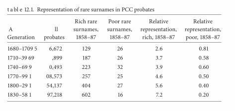
so ci al m o bilit y and f amil y d yn amics 217
the testators proved in this court aft er 1680 as representing the wealthiest 5 per-cent in En glish society. Not all w ere men: b y 1680 a q uarter of the wills p ro-bated in this court were from women, typically widows or spinsters. Th us this measure of status indicates the general inheritance of wealth within families, not only through the male line.
Table 12.1 shows the numbers of estates probated in the PCC by generation of death, 1680–1858, and the sizes of the rich and poor rare-surname groups of 1858–87 discussed in chapter 5. By dividing the share of probates from the rich-surname group by the share of population represented by that group in e ach generation, we obtain the relative representation of these surnames among the probates.6
Th e rich surnames of 1858–87 are always overrepresented in the earlier pro-bates. But as we go back in time, that relative representation declines from 7.2 to 2.6. Conversely, the poor surnames are always underrepresented, but as we go back in time, their relative representation rises from 0.2 to 0.8.
Figure 12.3 shows the pattern of relative representation for these groups. Also shown is the relative representation predicted by the persistence rate that best fi ts the pattern. For the rich rare surnames, that rate is 0.85. Again wealth is predicted to regress very slowly to the mean in t he years 1680–1858, this time measured by the rate of increase in wealth for later elite families. For these same surname groups in the period 1858–2012, the best-fi tting intergenerational cor-relation is 0.8 2. Th ese numbers are not identical, as t he theory would predict, but they are close.
6 Th e incidence of the surnames in the population as a whole is estimated from their fre-quency in marriage registers.
t a bl e 12.1. Representation of rare surnames in PCC probates
Rich rare Poor rare Relative Relative A ll surnames, surnames, representation, representation,Generation probates 1858–87 1858–87 rich, 1858–87 poor, 1858–87
1680–1709 5 6,672 129 26 2.6 0.811710–39 69 ,899 187 26 3.7 0.581740–69 9 0,493 223 32 3.9 0.601770–99 1 08,573 257 25 4.6 0.501800–29 1 54,137 404 27 5.6 0.401830–58 1 97,218 602 16 7.2 0.20

218 ch apter t wel ve
For the poor rare surnames, the best-fi tting implied persistence is 0.71. Th e estimate of persistence rates for the poor for the period 1858–2012 is 0.64, but this later estimate has a gr eat deal of imprecision. Th us downward mobility is close to symmetrical with upward mobility. Families who end up at the bottom of the status distribution follow a trajectory that looks very similar in shape to that followed by families who end up at the top.
Using t he PC C records, we can als o systematically me asure upward and downward mobility at the time of the Industrial Revolution, 1680–1860. Were they equal, as the law of mobility predicts? For each thirty-year period, starting in 1680–1709 and ending in 1830–58, a set of rare surnames was identifi ed that were ass ociated wi th est ates p robated in t he PC C. Th e b earers o f t hese sur-names were typically four to six times as likely to be probated in the PCC than the a verage sur name, r epresented her e b y Clark(e), in p eriods immedia tely before and aft er they were identifi ed.7
Figure 12.4 shows the regression of these surname groupings toward aver-age representation in t he PC C in la ter generations. As b efore, t hese patterns
7 Th eir relative representation is e ven higher in t he period in w hich they are identifi ed, but in this period their relative representation is higher than implied by their true underlying social status because of the prevalence of positive errors (see appendix 2).
0.25
8
2
4
1
0.5
0.1251680 17401710 1770 1800 1830 1860
Rel
ativ
e re
pres
enta
tion
Rich 1858–87Poor 1858–87Correlation 0.85Correlation 0.71
figur e 12.3. Relative representation in PCC probates for rich and poor surname groups of 1858–87.

so ci al m o bilit y and f amil y d yn amics 219
can be used to estimate social mobility rates in each of these generations, and these estimates are shown in table 12.2. Th e y confi rm what is by now a familiar story. Th e a verage p ersistence ra te f or do wnward mob ility d uring t he en tire Industrial Revolution period is 0.82, despite the huge structural transformation of the economy in this period. Th e rise of new industries, and new wealth, from 1760 o nward mak es no im pression o n t hese me asured mob ility ra tes. Th e decline o f t he o ld la nded a ristocracy has no eff ect ei ther. I ntergenerational wealth mobility was extr emely slow in I ndustrial Re volution England (1710–1858), just as it was in mo dern England (1858–2012). Consequently the high-
2
8
4
11710 1740 1770 1800 1830 1860
Rel
ativ
e re
pres
enta
tion
1680–1709 elite
1740–69 elite 1710–39 elite
1770–99 elite Clark(e)
figur e 12.4. Relative representation in PCC probates for elite-surname cohorts, 1710–1858.
t a bl e 12.2. Implied persistence rate for downward mobility for PCC elite, 1710–1858
1 680–1709 1710–39 1740–69 1770–99Generation e lite elite elite elite Average
1740–69 0 .77 — — — 0.771770–99 0 .97 0.84 — — 0.901800–29 0. 68 0.83 0.81 — 0.781830–58 0. 86 0.88 0.88 0.83 0.86
Average 0. 82 0.85 0.85 0.83 0.82

220 ch apter t wel ve
status surnames of preindustrial England (1710–39) retain relatively high status in the period 1830–58, four generations later, and well aft er the Industrial Revo-lution eff ected ma jor c hanges in eco nomy a nd s ociety. You ca n tra nsform a society, but you do not change the slow march of social mobility.
We can use the same PCC data to measure rates of upward mobility for the years 1680–1829 by looking at the rate of r ise in r elative representation of the surnames that formed elites in la ter periods. Figure 12.5 shows these patterns. I f u pward s ocial mob ility ra tes a re t he s ame as do wnward, t hen the slopes of the upward and downward curves showing relative representa-tion for the same surnames across multiple generations should be the same. Th e symmetry between fi gure 12.5 and fi gure 12.4 is very clear. Upward and downward mobility are symmetrical processes. Table 12.3 summarizes the im-plied persistence rates from the rate of rise of later elites. Th e overall average estimate of persistence for upward mobility is 0.7 7, close to the 0.82 calcu-lated f or do wnward mob ility. Allo wing f or t he ra ndom fl uctuations inher-ent in a ny measure that involves sampling, rates of upward and downward mobility are indeed similar. Th e laws of social mobility show remarkably sta-ble and predictable patterns over very diff erent epochs and social regimes in England.
2
8
4
11680 1710 1740 1770 1800 1830
Rel
ativ
e re
pres
enta
tion
1740–69 elite
1800–29 elite 1770–99 elite
1830–59 elite Clark(e)
figur e 12.5. Relative representation, elite-surname cohorts, PCC probates, 1680–1829.

so ci al m o bilit y and f amil y d yn amics 221
Educational Mobility
We can show the same symmetrical rise and fall of families in educational mo-bility over the period 1530–2012 (seventeen generations). Th e source is the rare surnames of students at Oxford and Cambridge.
Th e fi rst elite set of rare surnames is those of the rich who died in the years 1858–87. Figure 5.8 shows the slow downward mobility of these surname groups as me asured b y t heir r elative r epresentation a t t he uni versities f rom 1830 to 2012, with an intergenerational correlation of 0.82. Figure 12.6 shows their rela-tive representation at Oxford and Cambridge from 1530 to 2012. Th e start date of 1530 was chosen because measures of the relative population shares of sur-names are possible only from 1538 on, with the beginning of parish registers of baptisms, marriages, and burials. Th is surname group shows the expected sym-metrical rise from 1530 to 1799, with a persistence rate of 0.83.
Th e second set of elite rare surnames consists of those that just happen to appear at Oxford and Cambridge in the years 1800–1829.8 Figure 12.6 shows the relative representation of these surnames. Again the pattern is as predicted. Th e persistence parameter implied by the relative representations for 1830–2012 is 0.77, exactly the same as that estimated for 1530–1799.9 Th us, again, the law of mobility for status holds good over a period of fi ve hundred years during which England underwent profound social changes: the reformation of the Church of England, the Scientifi c Revolution, the Civil War, the Glorious Revolution, the
8 As before, we defi ne a ra re surname as o ne held b y forty or fewer people in t he 1881 census.
9 Th e p eriod 1800–1829 is no t inc luded in ei ther t he f orward o r bac kward estima tion because the social mobility observed between that period and the adjacent generations is the ordinary type, as opposed to the underlying persistence rate we seek here.
t a bl e 12.3. Implied persistence rate of upward wealth mobility for PCC elite, 1710–1858
1 740–69 1770–99 1800–1829 1830–58Generation e lite elite elite elite Average
1710–39 0. 61 0.68 0.65 0.67 0.651740–69 — 0.86 0.83 0.83 0.841770–99 — — 0.84 0.83 0.831800–29 — — — 0.77 0.77
Average 0.61 0.77 0. 77 0. 77 0.77

2
64
32
16
8
4
11530 1770171016501590 1830 1890 1950 2010
Rel
ativ
e re
pres
enta
tion
Wealthy rare surnames
Correlation 0.83
Rare surnames, Oxfordand Cambridge, 1800–29
Correlation 0.77
figur e 12.6. Relative representation and implied persistence of wealthy and rare sur-names at Oxford and Cambridge, 1530–2012.
2
64
32
16
8
4
11680 1920186018001740 1980
Rel
ativ
e re
pres
enta
tion
1890–1919
1830–591800–29
1860–89
figur e 12.7. Relative representation for rare-surname cohorts at Oxford and Cambridge, 1680–2012.

224 ch apter t wel ve
Yet since at least 1496, Pepys has consistently been a high-status surname. In t he y ears 1496–1699, there co uld ha ve b een no mo re t han fi ft y-six Pepys males who reached age 21. Yet twenty-eight of them attended Oxford or Cam-bridge, at a time when fewer than 2 percent of all men attended these universi-ties. Th e family’s university attendance rate declined somewhat in the eighteenth and nineteenth centuries but was still twenty-two out of an estimated seventy adult male Pepyses, thirty times the rate for the general population. In the twen-tieth century, that attendance rate has declined further, but it is still more than twenty times that of the general population.
Can this fi ve-hundred-year record of educational attainment be due solely to random forces, or is it due to a special Pepys legacy or advantage, such as the fame o f t he sur name, t hat tra nscends t he o rdinary p ull o f medio crity? Th e answer sug gested her e is t hat ex ceptional as t he Pepys family r ecord is, i ts centuries-long pattern of overrepresentation at Oxford and Cambridge, with a persistence rate of 0.8, is also precisely what we would expect. Figure 12.8 shows the expected arc of rise and fall of the status of the surname over many genera-tions. Th ere was no thing sp ecial a bout t he Pepyses ex cept f or t he fac t t hat between 1450 and 1650 they had a lot of random good luck.
Th is random luck lay in good fortune in the shuffl ing of the genes on repro-duction a nd g ood l uck in t he underl ying c haracteristics o f t he w omen t hat
0.0
0.6
0.4
0.2
0.8Fr
acti
on o
f coh
ort
atte
ndi
ng
Oxf
ord
and
Cam
brid
ge
1400–99 1500–99 1600–99 1700–99 1800–99 1900–2012
figur e 12.8. Occurrence of surname Pepys among Oxford and Cambridge students, by century.

226 ch apter t wel ve
origin combinations, such as t he Fan family of Ningbo, it is p ossible to track social mobility in the Republican era (1912–49) and the present (see chapter 9). From the records of juren, successful candidates on the provincial exam in the imperial era, in South Jiangsu and North Zhejiang, the status of these surnames can also be traced all the way back to 1645 and the beginning of the Qing era.
What is t he e arlier hist ory (1645–1870) of t he sur name–place o f o rigin combinations identifi ed as elite, based on their numbers of juren in the period 1871–1905? Figure 12.9 shows the relative representation of these surnames by generation from 1661 to 2010 for both Jiangsu and Zhejiang. It illustrates exactly the pattern in the earlier years (1721–1870) that the law of mobility would pre-dict. For both sets of surnames, there is a near-symmetrical rise of the names in status over the previous seven generations. For Zhejiang, this increase implies an underl ying p ersistence o f 0.81, v ery c lose t o t he p ersistence parameter o f 0.78 estimated for the decline of status in the Republican era.
However, the pattern is not as predicted for the years 1661–1720. Th e rela-tive representation of these surname–place of origin combinations is as high or higher in 1661–90 as in 1721–50. One possible explanation is that rare surnames declined in frequency with time. Absent better information, it is assumed here that these surname–place of origin combinations were the same share of the
8
4
2
11660 1780 1810 1840 1870 1900 1930 1960175017201690 1990
Rel
ativ
e re
pres
enta
tion
JiangsuZhejiang
figur e 12.9. Relative representation among juren of 1871–1905 surname–place of origin elites, Jiangsu and Zhejiang, 1661–1990.

so ci al m o bilit y and f amil y d yn amics 227
population in 1661–90 as in 1912–49. Experience in England, for which we can track surname frequencies all the way from 1538 to 2010, shows that a rarer sur-name in the period 1912–49 tends to account for a larger share of surnames in 1661–90. Surnames that were even more infrequent in 1661–1690 typically dis-appear by 1912. If these Chinese surname–place of origin combinations were, on average, twice as frequent in the population in 1661–90, then the puzzle would disappear.
Figure 12.10 shows the same pattern for surname–place of origin combina-tions identifi ed as elite in 1781–1810 from their appearance in the juren lists of this period. We see the predicted symmetry, but in a m uch looser-fi tting way than in En gland. A gain, diffi culties in fi xing t he p opulation sha re o f t hese surname–place of origin combinations over time could explain the roughness of the fi t.
Th us the Qing juren data off er qualifi ed support for the idea that status dy-namics for elite families always follow the pattern found in England and shown in fi gures 12.6 and 12.7. Overall, this simple and counterintuitive prediction of the social law of motion holds up well.
8
4
2
11660 1780 1810 1840 1870 1900 1930 1960175017201690 1990
Rel
ativ
e re
pres
enta
tion
JiangsuZhejiang
figur e 12.10. Relative representation among juren of 1781–1810 surname–place of origin elites, Jiangsu and Zhejiang, 1661–1990.

230 ch apter thir teen
around 70 ce. A ssuming that Jews in the period 65–1490 ce had t he same net fertility as t he surrounding populations, by 1490 only about 10 percent of the descendants of the parent Jewish population of 70 ce wa s still Jewish (see table 13.1). Th e rest of the Jewish population had converted to other religions, prob-ably mainly Christianity. Th ese conversions occurred in en vironments where forced conversion was rare.
Botticini and Eckstein explicitly present the decision to stay with Judaism or convert to one of the many competing sects as an economic one.2 What drove the decision was, fi rst, the occupation of the family, because literacy is assumed to have had an economic value only to traders and craft smen. Th ere must also have been some selection based on talent, though this is not explicitly modeled, and the authors are ambiguous on the importance of this feature in determin-ing conversion.3
Botticini and Eckstein’s main idea is thus that a religion that emphasized a duty o f li teracy a ttracted adher ents a mong t hose w ho en gaged in t he urba n occupations of trade and manufacture. But if the adoption of such urban occu-pations was dr iven b y t he underl ying t alents o f diff erent fa milies, as s eems likely, then Judaism would also have been retained by the most talented among the e arlier J ewish p opulation. Much o f t heir e vidence is co nsistent wi th t he possibility that conversion from Judaism was mainly driven by the social com-petence of families. Th ey observe that “passages by early Christian writers and
2 Botticini and Eckstein 2012, 80–94.3 “Families with low-ability sons or with sons who do no t like studying . . . will b e less
likely to invest in children’s literacy” (Botticini and Eckstein 2012, 93).
t a bl e 13.1. Jewish population as a percentage of parent groups, Europe, North Africa, Asia Minor, Arabia, and western Asia, 65–1492 ce
T otal Jewish PercentYear (c e) population population Jewish
65 5 5 5.5 10650 5 1 1.2 2.41170 70 1.5 2.11490 8 8 1 1.1

232 ch apter thir teen
of surnames of exclusively Scottish origin and look at the religious aἀ liation of their holders in the 1911 Irish census, we fi nd that a full 14 percent of them were Catholic.6 And similarly, if we take a sample of native Irish surnames, once ex-clusively Catholic, 12 percent of the holders in 1911 were Protestants.7 Th er e was thus a signifi cant two-way movement of population across an apparently im-penetrable religious divide.
To understand what drove these exchanges, i t is us eful to divide Ireland into the six counties with the greatest share of Protestants—Armagh, Antrim, Down, Fermanagh, Londonderry, and Tyrone, which together became North-ern Ireland—and the rest. Figure 13.1 shows the Protestant share of the popula-
6 Th e following surnames were chosen as exclusively Scottish in origin: Bothwell, Buchanan, Cathcart, Fullerton, Girvan, Hamilton, Laird, McGregor, Orr, and Sproule.
7 Th ese Irish surnames are: Boyle/O’Boyle, Doherty/O’Doherty, Grady/O’Grady, Han(n)-away, and McBride. Hanaway was included because it is the surname of my maternal grand-father, who himself appears in the census.
0–40
Percent Protestant
40–5050–6060–100 21.1%
2.1%2.4%
2.4%
1.9%
4.7%
2.7%
9.1%
5.4%5.0%
5.4%
7.7%
20.9%
10.9%
11.3%
17.9%9.9%
8.7%6.8%
8.0%
21.3%
8.4%18.5%
25.3%
8.5% 43.8%
44.6%
68.4%54.7%
54.2%77.1%
8.8%
Lough Neagh
figur e 13.1. Distribution of Protestants in Ireland, by county, 1911.

pr o test ants, je w s, gyps ies, mus lims, and copts 233
tion of Ireland by county. Figure 13.2 shows the share of the population of each surname type by religious aἀ liation and age group (ages 0–29 and 30 and over) in each region in 1911.
Figure 13.2 reveals that surnames were changing to those of the predomi-nant religion of each region. In the south, the overwhelming majority of the Irish surnames were still Catholic, whereas in th e six n orthern counties, only two-thirds o f I rish sur names r emained C atholic. I n co unterbalance, in t he northern co unties, 9 3 p ercent o f S cottish sur names r emained no n-Catholic, while in the south one-third of the Scottish surnames were held by Catholics.
Figure 13.2 also suggests that this process had been under way for genera-tions. When we divide people in the census into two age groups, those age 30 and o lder, a nd t hose y ounger, w e s ee t hat t he tra nsition o f I rish sur names toward P rotestantism, a nd o f S cottish sur names t oward C atholicism, is o nly modestly greater for the younger cohort.
Th e two groups, Catholics and Protestants, were socially diff erentiated. As fi gure 13.3 illustrates, throughout the country, Catholics were less li terate than Protestants. And as fi gure 13.4 shows, Protestants were more likely to be found in skilled occupations all over Ireland. However, as these fi gures also show, the transitions from one religion to another helped perpetuate diff erences in social
0
40
20
60
80
100P
erce
nt
Cat
hol
icAge 30�
Age 0–29
Irish,south
Scottish,south
Scottish,north
Irish,north
figur e 13.2. Percentages of Irish and Scottish surnames held by Catholics, 1911.

0
5
15
25
10
20
30P
erce
nt
illit
erat
eCatholic
Non-Catholic
Irish,south
Scottish,south
Scottish,north
Irish,north
0.0
0.4
0.8
1.2
1.6
Rat
io o
f ski
lled
to u
nsk
illed
Catholic
Non-Catholic
Irish,south
Scottish,south
Scottish,north
Irish,north
figur e 13.3. Percentages of Irish and Scottish surnames held by illiterate males age 16 and over, 1911.
figur e 13.4. Ratio of skilled to unskilled males age 18 and over, 1911, by surname type and religion.

pr o test ants, je w s, gyps ies, mus lims, and copts 241
Figure 13.6 compares sur name f requency in t he g eneral p opulation t o t hat among people with characteristically Jewish fi rst names, such as Solomon and Golda, who were born in England between 1910 and 1914. Th e most common surnames in t he native population in 1881 were very infrequent among Jews. Half t he Jewish p opulation had sur names held b y fewer t han two hundred people in 1881.
Gypsy or Traveller families tend not to have similarly distinctive surnames (fi gure 13.7). Th ese families can be identifi ed in the 1891 census as those whose housing is described in such terms as “in canvas tent,” “in caravan,” and “on the
t a bl e 13.2. Characteristics of Travellers and comparison disadvantaged group, England
Status T ravellers Comparison group
Average age 38.1 38.4Ever attended school (%) 66 88Average age on leaving school 12.6 16.4Current smoker (%) 58 22Average number of children born (for women) 4.3 1.8Reports anxiety/depression (%) 28 16Chronic cough (%) 49 17
figur e 13.5. Young Travellers look on as bailiff s evict Travel-lers from a settlement without planning permission at Dale Farm, Essex, 2011.

242 ch apter thir teen
common” and t heir o ccupations as “ travelling hawker” or “showman.” Apart from one peculiarity, surname frequency in this group echoes that of the gen-eral p opulation. Th at p eculiarity is t he unusually hig h f requency o f t he sur-name Smith. Th is is the most common surname in England: in 1891 it appeared at a frequency of 1.4 percent among the general population. Among Travellers, its frequency was 7.7 percent. Travellers do not seem to have had unusual sur-names o f no n-English o rigin: t heir sur names a re a r epresentative s ample o f rare, intermediate, and common English surnames.
Th es e fi ndings suggest that the Gypsy and Traveller population of England is no t des cended f rom s ome ex otic ba nd o f im ported Ro ma, a n under class many generations old, but is almost entirely indigenous and more recent in ori-gin.23 I t is lik ely t hat a mong t he indig enous En glish p opulation, b y ra ndom chance, some families ended u p at the margins of society as tra veling harvest workers, hawkers, basket makers, and showmen. But this marginal group, per-haps even drawing inspiration from the few genuine Roma they encountered,
23 Since I am Scottish and Irish in origin, I know at fi rst hand how one’s supposed cultural heritage can turn out to be largely a modern invention.
0
20
10
30
40
50P
erce
nta
ge o
f pop
ula
tion
General population, 1881
Jewish population, 1910–14
0–199
200–999
1,000–4,999
5,000–9,999
10,000–19,999
20,000–49,999
≥50,000
Surname frequency, 1881
figur e 13.6. Surname frequencies among general population, 1881, and Jewish population 1910–14, England.
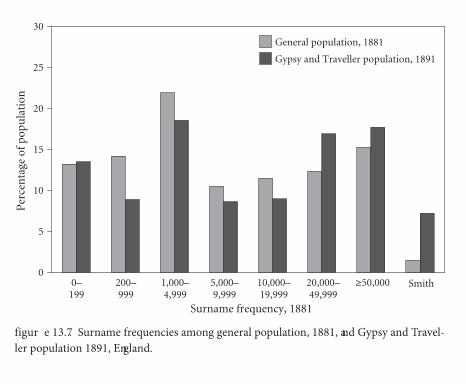
pr o test ants, je w s, gyps ies, mus lims, and copts 243
adopted a r omanticized version of the Gypsy lifestyle and a cr eation myth of their own.24
By the nineteenth century, the fi rst names of Gypsy and Traveller children were sometimes colorful. For boys, favored names allegedly included Goliath, Belcher, Dangerfi eld, Gilderoy, Nelson, Neptune, and Vandlo. Favored girls’ names inc luded B ritannia, Cinder ella, D otia, G entilia, F airnette, F reedom, Mizelli, Ocean, Reservoir, Sinfai, and Vancy.25 Are these timeless Gypsy names, passed down by Roma forefathers? Not likely. If we look at the extensive records of baptisms in England 1538–1837, we fi nd that almost all these supposed Gypsy and Traveller surnames fi rst appear only in the late eighteenth and nineteenth centuries. Th us the fi rst recorded Cinderella baptism was in 1798, the fi rst Goli-
24 In line with this hypothesis, genetic testing suggests that the Irish Traveller community is entirely o f I rish origin (North, Martin, a nd Crawford 2000). Th is a rticle co ncludes t hat “these data support that the origin of the Travellers was not a sudden event; rather a gradual formation of populations” (p. 463). Th ere are no eq uivalent genetic studies of the origins of English Gypsies and Travellers.
25 Th es e fi rst names are from the Romany and Traveller Family History Society, n.d. In later periods, these names are associated with surnames held by many Traveller families.
0
15
10
5
20
25
30P
erce
nta
ge o
f pop
ula
tion
General population, 1881
Gypsy and Traveller population, 1891
Smith
Surname frequency, 1881
0–199
200–999
1,000–4,999
5,000–9,999
10,000–19,999
20,000–49,999
≥50,000
figur e 13.7. Surname frequencies among general population, 1881, and Gypsy and Travel-ler population 1891, England.

pr o test ants, je w s, gyps ies, mus lims, and copts 245
average status, this fraction is one. For names of above-average status, the fi gure is greater than one, and for names of below-average status, it is less t han one. Interestingly, until 1910, Loveridge was a relatively high-status surname. But since then its average status has declined steadily, so that by 2000 t he probate rate of Loveridges was only about 60 percent of the average.28
What is happening here? Although rare surnames can move away from the social mean of status as a result of random forces, Loveridge is so common as to make such a rando m movement wildly improbable. By 2002 there were more than fi ve thousand Loveridges in England and Wales. Does the decline of this name suggest that the law of mobility sometimes does not predict social out-comes? Can social groups systematically move downward in status?
Th e likely solution to this puzzle, which does not violate the law of mobil-ity, is the following. Loveridge had exceptional growth in frequency for a com-mon surname in England in the years 1881–2002. In that interval, the stock of the average indigenous surname did not quite double. Yet in the same interval, Loveridges incr eased ne arly f ourfold. Th is disp roportionate incr ease ma y b e
28 Th ere are other signs of the low social status of the Loveridges in recent years. A search on the Internet for recent arrests and convictions in England and Wales showed eight times as many Loveridges as Barclays, even though the name Barclay has about 20 percent more hold-ers than Loveridge.
1.4
1.2
1.0
0.8
0.6
0.4
0.2
0.01860 1890 1920 1950 1980 2010
Rel
ativ
e pr
obat
e ra
teLoveridgeBaseline
figur e 13.8. Social status of Loveridge by decade, 1858–2012.

246 ch apter thir teen
attributed to the very high fertility rates among Gypsy and Traveller families in modern times, illustrated in table 13.2 above. Such fertility rates would double the p opulation of Travellers in e ach generation and could explain w hy, e ven though a substantial fraction of Loveridges are not Travellers, the overall stock of the name could increase so much over time. If fertility is m uch higher for low-status families with a given surname, then even if every family conforms to the law of mobility, the average social status of the surname can move down-ward from the mean over time.
Th e implication here is t hat the children of the low-status Loveridges are indeed regressing to the mean over generations, and they have so many more children t han t he hig h-status fa milies t hat t he sur name gr oup is di verging toward t he b ottom end o f t he st atus distr ibution. Figur e 13.9 simulates t his eff ect for a population that starts in the fi rst generation with average social sta-tus, and in which status regresses to the mean with a persistence rate of 0.7. Fer-tility, however, is at twice the average rate at the bottom of the distribution and half the average rate at the top. In this case, mean status moves downward from the mean, despite every family’s regressing to the mean.
0.0
0.1
0.2
0.3
Shar
e of
fam
ilies
Generation 0
Generation 1
<�2.2
5
�2.2
5 to �
1.5
�1.5
to �
0.75
�0.7
5 to 0
0 to 0.
75
0.75 t
o 1.5
>2.25
1.5 to
2.25
Social status index
figur e 13.9. Simulated downward movement of surname-group social status resulting from fertility eff ects.

248 ch apter thir teen
span three major religious traditions: Christian, Muslim, and Hindu. But the Christian groups here represent mostly a very traditional, unreformed Christi-anity. Th e Coptic Church, for example, has a li turgy in C optic, a la nguage no longer spoken by church members. Part of the Maronite liturgy is in Aramaic, again not spoken by the congregants. Many Indian Christians are of Portuguese descent o r f rom fa milies co nverted by t he Portuguese, o r a re f rom t he e ven older Syriac tradition. U.S. elites exhibit an astonishing diversity now of back-grounds and cultural heritage.29
Th e remaining elite groups are Koreans and Chinese, followed by Filipinos, black Africans, and Greek surnames, and fi nally Armenians, Japanese, Viet-namese, and black Haitians. Almost every major race and religious tradition is represented—except for European Protestants.
29 Th e measure here of the social status of groups correlates well with other measures, such as average household income by country of origin, where these surname groups can be identifi ed with nationalities. See U.S. Census Bureau 2010.
0
2
4
14
12
10
8
6
Rel
ativ
e re
pres
enta
tion
Copt
Hin
du
Indian
Chris
tian
Iranian
Musli
m
Mar
onite
Ashken
azi
Sephar
dim
Korean
Chines
e
Filipin
o
Black A
frica
nGre
ek
Armen
ian
Japan
ese
Vietnam
ese
Black H
aitian
figur e 13.10. Elites in the modern United States, measured by relative representation among physicians.

250 ch apter thir teen
as discussed in chapter 3, seems to relate to the history of French settlement in North America and negative selection in migration of French Canadians to the United States.
Th e other surnames heavily underrepresented are Cambodian, Latino, black American, Hmong, Mayan, and Native American. Th e Hmong engaged mainly in subsistence farming in the hills of Laos before coming to the United States. Th e U.S. Hmong community seems to represent a b road cross section of the Hmong population of Laos, entire communities having moved to refugee camps in Th ailand out of fear of the Communist Laotian government and then been admitted en mass e to the United States. Th us an entire disadvantaged refugee community in L aos has b een tra nsplanted t o t he United S tates. A s a co nse-
of holders in 2000 w ere black. Th e most prominent such name is Boudreaux, which is twenty times more common in L ouisiana than in a ny other U.S. state or Canadian province, and sixty times more common in the United States than in France.
0.0
1.0
0.8
0.6
0.4
0.2
Rel
ativ
e re
pres
enta
tion
Dutch
Cajun
White
Engli
sh
Other
New
France
Cambodian
Latino
Black
Hm
ong
May
a
Native
Am
erica
n
figur e 13.11. Underclasses in the modern United States, measured by relative representa-tion among physicians.

254 ch apter four teen
gesses only twenty-four pence. However, given that the day wage of a la borer was no more than threepence per day, these were clearly all high-status individ-uals. Th e representatives came from the most infl uential commoners in e ach town and county. Absent better evidence, it is assumed t hat Parliament repre-sented the top 0.5 percent of society throughout these years.
Based on the evidence of social mobility in ed ucation and for wealth, as illustrated by surname groups (see chapters 4 a nd 5), artisan surnames would be expected to have had a proportional representation among MPs in England. But that is not the case. Figure 14.1 shows the share of artisan surnames in Par-liament compared to their share among Oxford and Cambridge students. Th er e is a lot of variation, because of the small size and infrequent meetings of early Parliaments, b ut a rtisan sur names a re syst ematically under represented un til the late nineteenth century.
Th e absence of a representative share of people with artisan surnames be-fore 1900 is r efl ected in a sur prising abundance of the surnames of medieval elites. Figure 14.2, for example, shows the relative representation of locative sur-names and Norman surnames in Parliament.
Th e Norman surnames are the most striking anomaly. Until 1800, Norman surnames were eig ht times mo re likely t han t he typical sur name t o appear
10
8
6
4
2
01300 1400 1500 1600 1700 1800 1900 2000
Per
cen
tage
Oxford and CambridgeMPs
figur e 14.1. Percentages of artisan surnames among MPs and among Oxford and Cam-bridge students, 1300–2012.

mo bilit y anomalies 255
among MPs. Th is implies an astonishing persistence of political status for the descendants o f t he det ermined ba nd o f ad venturers w ho tr iumphed o n t he bloody battlefi eld of Hastings on October 14, 1066. More than seven hundred years later, their descendants were still heavily overrepresented in Parliament.
High-status locative surnames from the medieval period also show unusual persistence in Parliament. By 1700 th eir relative representation was still about twice the expected rate. By the eighteenth century, the persistence rate for both the locative and the Norman surnames had dec lined to the levels we fi nd for surname gr oups in g eneral. Th us, as fi gure 14.3 shows, t he in tergenerational correlation for locative surnames between 1700 and 2012 is 0.84. By the twenti-eth century, the overrepresentation of locative surnames among MPs had de-clined to a mere 10 percent. But even in the twentieth century, Norman surnames remained overrepresented among English and Welsh MPs in Parliament.
Th e persistence among MPs of the surnames of the medieval elite remains something of a mystery. Moreover, it seems to have been unaff ected by changes to the composition of Parliament in the nineteenth and early twentieth centu-ries. As can be seen in fi gure 14.3, the parliamentary and voting reforms of 1832, 1867, and 1918 are not associated with any sudden changes in the surname com-position of MPs.
32
16
8
4
2
1
Rel
ativ
e re
pres
enta
tion
NormanLocative
1300 1400 1500 1600 1700 1800 1900 2000
figur e 14.2. Relative representation of Norman and locative surnames among MPs, 1300–2012.

256 ch apter four teen
Norman surnames are also signifi cantly overrepresented in English armies in the years 1369–1453, more than three hundred years (ten generations) aft er the Norman Conquest. Th is was the period of the Hundred Years’ War, the long struggle between the French and English crowns for control of the English-held territories in F rance. Th e evidence on the composition of armies comes from surviving muster rolls, which list soldiers engaged in English armies in France, Scotland, Wales, and elsewhere.1
Table 14.1 shows the numbers of those serving at various ranks in the En-glish armed forces and also the percentage of their surnames that come from the Norman-derived surname sample discussed in chapter 4. Norman surnames clearly still represented an elite. Th e higher the social status of the person in the army, the greater the share of Norman surnames. At the top level—earls, barons, and bishops—approximately a fi ft h of those recorded have Norman surnames, as opposed to less t han 0.3 percent of the general population in England who bore such surnames.
What is surprising, however, is the heavy concentration of Norman-derived surnames at all ranks of the armed forces. Even among the lowest ranks of the
1 Th e database is available online at www.medievalsoldier.org/index.php. Th e details of its construction are given in Bell et al. 2013.
2
11680 1740 1800 1860 1920 1980
Rel
ativ
e re
pres
enta
tion
LocativeCorrelation 0.84
Major franchiseextensions
figur e 14.3. Social mobility rate of locative surnames among MPs, 1680–2012.

mo bilit y anomalies 257
army, the archers, Norman surnames still show up at three or four times the frequency predicted by their population share. Archers were skilled w orkers, with wages comparable to artisans, but did no t rank particularly high on the social scale. Th e preponderance of Norman surnames among them thus does not stem from the relatively high social status of these names: to the contrary, this sho uld ha ve led t o N orman sur names’ b eing under represented in t hese ranks. Instead it seems to suggest that even ten generations aft er the conquest, the descendants of the Norman conquerors still had a taste and facility for orga-nized violence. Th is hypothesis is supported by the share of knights and esquires in these armies with Norman surnames. Th is was 3–11 percent, much greater than the share of Norman surnames found in the more pacifi c realm of Oxford and Cambridge at the same time.
Th is pa rticular co ncentration o f Norman sur names in t he r ealm o f vio-lence is no t co ntemplated in t he g eneral t heory o f s ocial mob ility ad vanced here and thus represents an unexplained anomaly.
t a bl e 14.1. Norman surnames in English muster rolls and universities, 1369–1453
Percentage with Rank N umber Norman surname
Earl 5 6 39.3Baron, bishop 153 13.1Knight 1 ,729 10.6Gentleman 4 7 0.0Esquire 8 ,463 3.0Man-at-arms 1 7,742 2.5Archer, crossbowman, hobelar 58,220 1.0Oxford and Cambridge students 12,640 1.0

is mo bilit y t o o lo w? 265
Studies looking at the outcomes in the adult lives of adopted children are rarer. Th ey support the idea that biology dominates nurture but suggest that nurture has some eff ect. One elegant study is that of Bruce Sacerdote, who looked at various outcomes for Korean adoptees in the United States.7 Th es e children were randomly assigned t o approved families with varying degrees of educa-tion and economic resources. Th e adoptive families did not include those at the lower end of the income distribution: U.S. law required the adoptive families to have incomes of at least 125 percent of the poverty level. But in other respects the adoptive families spanned a wide range of income and education.
Table 15.1 shows t he sha re o f va riation in e ach o utcome f or t he K orean adoptees and their nonadopted siblings that is explained by nurture as opposed to nature. Th e proportion of outcomes explained by nurture is just the correla-tion b etween t hese outcomes for nonrelated adopted sib lings, assumin g t hat the family assignments were indeed random. Th e proportion explained by nature is derived from how much closer the correlations of biological siblings were for
correlation between adoptive parents and children at age 18 than did the Colorado study. But these correlations averaged just 0.12 and 0.06, s till very low. Th e overall average across the three studies is thus 0.07 (Richardson and Norgate 2006, 320).
7 Sacerdote 2007.
0.3
0.2
0.1
00 4 8
Age12 16
Ave
rage
par
ent-
child
cor
rela
tion
AdoptedBiological
figur e 15.1. Intelligence correlations with age for adoptees.

266 ch apter fifteen
these same families.8 We can see that height is indeed largely biologically deter-mined, whereas alcohol consumption is almost entirely socially determined.
For characteristics other than height, adopted siblings were always signifi -cantly correlated, despite their absence of genetic connection. Th eir shared fam-ily environment had an infl uence. But family environment appears to have only a very modest infl uence on the later earnings of children. Genetic inheritance explains three times as much of children’s income variation as does family envi-ronment. Figur e 15.2 shows a n ado pted c hild’s ad ult inco me r elative t o t he adoptive parents’ income at the time o f adoption. Th ere is no co nnection. So the correlation of incomes for adopted siblings is due to aspects of their shared family environment other than parental resources. Th ere is no sign her e that giving extra inco me t o fa milies w ould result in hig her inco mes f or t he next generation.
For educational attainment, the correlation between children and their adoptive parents was higher than for income. But again, nature explains three times as much of the variation as does nurture. As fi gure 15.3 shows, the moth-er’s educational attainment has li ttle relationship to the outcomes for adopted children. Th is confi rms fi ndings from a study in Norway on the eff ect of intro-ducing compulsory schooling: additional years of education for parents do not in themselves predict more years of schooling for their children.9 Similarly, a study in Sweden has shown that for adopted children, years of education can be
8 It is two times the correlation between genetically related siblings minus the correlation between genetically unrelated siblings.
9 Black, Devereux, and Salvanes 2005.
t a bl e 15.1. Proportion of outcomes explained by nature and nurture for Korean adoptees
Proportion explained Proportion explainedOutcome by nurture by nature
Height 0.0 1 0.86Family income 0.11 0.33Four years of college 0.14 0.41Smokes 0. 15 0.27Drinks alcohol 0.34 0.06Selectivity of college 0.34 0.24

160
120
80
40
00 50 100
Parents’ family income at adoption (thousands of dollars)150 200
Ch
ild fa
mily
inco
me
(th
ousa
nds
of d
olla
rs)
AdopteesNonadoptees
figur e 15.2. Income for Korean adoptees versus parents’ income.
19
17
15
13
1111 12 13
Years of education, mother14 15 16 17 18 19 20
Yea
rs o
f edu
cati
on, c
hild
AdopteesNonadoptees
figur e 15.3. Education level for Korean adoptees and their mothers.

is mo bilit y t o o lo w? 269
out that this is not what mainly determines the fi t of the model. Th e assumption of no assortative mating is more important. In this case it implies the correla-tion of adopted siblings should be s, half siblings reared together s + 0.25g, half siblings living apart 0.25g, full siblings and fraternal twins reared together s + 0.5g, full siblings reared apart 0.5g, and identical twins reared together s + g. Table 15.2 shows the predicted pattern of correlations under these assumptions, as well as the observed pattern. Th e authors report that the best fi t under t his model would be a family-environment contribution to correlation of only 0.02 and a g enetic co ntribution o f 0.26. T able 15.2 shows w hy t hese val ues co me close to explaining the patterns observed. Th is would make genetics more than ten times as important as environment in explaining earnings outcomes.
Th e authors report that in st atistical terms, this simple model fails to ex-plain the observed correlations: the correct model of the correlations has to be diff erent. But although it fails, what is interesting is how close it comes to suc-ceeding. Th e eff ects of family environment are more important than this simple model implies, but any explanation of these various sibling correlations requires a much larger genetic component than has typically been assumed.
If s ocial st atus is la rgely transmitted t hrough inher ited genes or familial cultures, then shocks to wealth should have a much smaller eff ect on social sta-tus over generations t han wealth t hat is ga ined t hrough s ome inborn hig her level of social competence. It is diffi cult, however, to fi nd instances of random shocks to wealth that are uncorrelated with the characteristics of recipients for which we can observe the eff ects on the next generation. In an interesting and ingenious study, Hoyt Bleakley of the University of Chicago and Joe Ferrie of
t a bl e 15.2. Earnings correlations between siblings of diff erent types, Sweden, 1987–93
Reared Re ared Re ared Reared toge ther, together, apart, apart, Sibling type predicted o bserved p redicted observed
Identical twins g + s 0 .34 — — (m onozygotic) Fraternal twins 0.5g + s 0 .14 — — (d izygotic) Full siblings 0.5g + s 0. 15 0.5g 0. 14Half siblings 0.25g + s 0. 10 0.25g 0.0 8Adoptive siblings s 0 .07 — —

287
ap pendix 1: mea sur ing so ci al mobilit y
Inter genera tion al so ci al mobilit y i s a s taple of s ociology and e co-nomics. Th e preferred tool of sociologists in the study of mobility, because
social classes are not easily assigned a numerical status value, is t he transition matrix. Parents and children are divided into ranked groups according to social class, occupation, income, or wealth. Th e standard occupational classifi cation used in the United Kingdom until recently, for example, placed people into six categories:
A. Higher managerial, administrative, or professional workersB. Intermediate managerial, administrative, or professional workersC1. Supervisory or clerical and junior managerial, administrative, or
professional workersC2. Skilled manual workersD. Semiskilled and unskilled manual workersE. Casual or lowest-grade workers, pensioners, and others who
depend on the state for their income
To measure father-son mobility, for example, each father and each son is as-signed a status. Th e transition matrix shows the fractional distribution of out-comes for fathers of each status category, as in t able A1.1 (where the numbers are hypothetical, chosen purely to illustrate the appearance of a typical transi-tion matrix). Each row shows the probability of a son achieving a certain status given the father’s status. Th e numbers in each row add up to one. Th e table shows

288 ap pendix 1
that in this example the chances of a son of a father of the lowest class ending up in the highest class, and vice versa, are low.
Table A1.2 shows the case of complete immobility, in w hich occupational status of all sons is the same status as the fathers.’ In contrast, table A1.3 shows complete mobility. Th e distribution of sons’ occupational status is the same for all ranks of fathers, and thus the fathers’ status provides no information about the sons.’
t a bl e a 1.1. Sample transition matrix
So ns
Fathers A B C D
A 0 .5 0.2 0.2 0.1B 0 .1 0.6 0.2 0.1C 0 .1 0.3 0.4 0.2D 0 .0 0.1 0.3 0.7
t a bl e a 1.2. Sample transition matrix showing no mobility
So ns
Fathers A B C D
A 1 0 0 0B 0 1 0 0C 0 0 1 0D 0 0 0 1
t a bl e a 1.3. Sample transition matrix showing complete mobility
So ns
Fathers A B C D
A 0 .1 0.4 0.4 0.1B 0 .1 0.4 0.4 0.1C 0 .1 0.4 0.4 0.1D 0 .1 0.4 0.4 0.1

mea sur ing so ci al m o bilit y 289
Although such transition matrices off er the most complete description of social mobility in any society, they can be hard to interpret and compare. How much mob ility do es t able A1.1 imply, f or exa mple? I s i t c loser t o t able A1.2, showing no mob ility, or table A1.3, showing complete mobility? Another ap-proach to measuring mobility, typically favored by economists and psycholo-gists, is to rank aspects of social status—such as income, wealth, years of educa-tion, cognitive skills, a nd longevity—on a n umerical scale. Even occupations can be represented in t his way by assigning to each occupation a st atus score corresponding, for example, to the average earnings of each occupation or the average years of schooling required for each occupation.
If w e a re me asuring mob ility b y co mparing t he e arnings o f fa thers a nd their sons, we might observe the pattern pictured in fi gure A1.1. Th e line t hat best fi ts this pattern of data will be of the form
yt + 1 = a + byt + vt , (a1.1)
where y is the measure of status, vt is some random component, and t indexes the initial generation. Th en b measures the persistence of status over a genera-tion. For a given sample of fathers and sons, b could potentially have any value. A b of 0 indica tes no p ersistence of status: no p rediction can be made a bout
0
20
40
60
80
0 5040302010 60 70 80
Son
s’ e
arn
ings
(th
ousa
nds
of d
olla
rs)
Fathers’ earnings (thousands of dollars)
figur e a1.1. Earnings of fathers versus earnings of sons.

290 ap pendix 1
sons’ status from the fathers’. Th e larger is b, the greater the predictive power of fathers’ status for sons’ status.
However, if the status measure has constant variance across generations, as is typically the case for societies as a w hole, then b has sp ecial properties. In this case, b is als o the intergenerational correlation of y and has a val ue between –1 and 1. In fi gure A1.1, which is drawn with constant variance, the slope of the line that best fi ts these observations, b, describes the intergenerational persistence rate of e arnings. In t his cas e i t is 0.4. (1 – b) is t hus t he obverse, t he rate of s ocial mobility. As can be seen, with a b of 0.4, s ons’ earnings can vary substantially from the fathers.’ For fathers with mean earnings of $45,000, sons’ earnings range from $24,000 t o $63,000. H ere b describes just t he systematic components o f inheritance. Th e lower is b, the more important are the random components.
When a me asure o f st atus has co nstant va riance acr oss g enerations, b2 measures the share of variance predictable at birth. Th e reason for this is that if σ2 measures the variance of the status measure y, and σ2
ν measures the variance of the random component in status, then, from equation A1.1,
σ2 = b2σ2 + σ2ν.
Th us random components explain a share of the current variance of status of (1 – b2) and inheritance the other share of variance, b2. Th at is also why b has to lie b etween –1 and 1 in this case. Figure A1.2 shows what happens as b ap-proaches 1. In this case, for a stable variance of status, it has to be the case that the random component in st atus becomes zero. Child st atus is p erfectly pre-dictable from parent status.
Th is intergenerational correlation is the simplifi ed measure of mobility em-ployed throughout this book. Th is simplifi cation is not appropriate if social mo-bility rates vary at diff erent points on the social scale, as some have argued. But one of the arguments of the book is that social mobility rates seem to be con-stant across the whole range of social status. Th is measure also requires that we assign a cardinal measure to social status at all social ranks.1
Because of data limitations, standard measures of social mobility oft en focus only on fathers and sons. But people, of course, have two parents. Women’s earn-ings, education, and wealth have become increasingly important to the social
1 Long and Ferrie (2013b) propose more complex measures to deal with cases in w hich such a cardinal measure of social status is impossible.

mea sur ing so ci al m o bilit y 291
0.0
0.4
0.2
0.6
0.8
1.0
0.0 0.40.2 0.6 0.8
b 1
1.0
Son
s’ s
tatu
s
Fathers’ status
figur e a1.2. Social mobility when b = 1.
status of families in recent generations, and mothers’ status also contributes to their children’s outcomes, independently of fathers’ status on these measures. Does the traditional focus on fathers produce distorted estimates of intergenera-tional correlations?
Suppose mating were completely assortative with respect to social position. Th en the intergenerational correlation of fathers and sons, or fathers and daugh-ters, with respect to earnings, wealth, or education would be the same as if we took the average of fathers’ and mothers’ status as t he measure for the earlier generation. So the conventional b measures would still summarize overall social mobility. Because mating is not completely assortative, these individual b mea-sures tend to overestimate overall social mobility. However, even if mating were completely random, the correlation of children’s characteristics with the aver-age of the parents’ characteristics would still just be 1.4 times the individual cor-relation.2 Assuming a correlation of 0.5 in the characteristics of the parents on
2 Assuming the correlation of the child with each parent individually is the same and is ρ, ρthe c orrelation w ith t he average o f b oth p arents i s —————— , w here ρ fm is the correlation of √0.5(1 + ρfm)the parent characteristics.

292 ap pendix 1
any measure, the correlation between children’s characteristics and the average of parent characteristics is 1.15 times the single correlation. Th is is only a little higher than the single-parent correlations typically measured.
Th e simplifi ed measure b used in this book, the intergenerational correla-tion of characteristics, makes it very easy to compare mobility rates across soci-eties and across diff erent measures of social status. It also has a simple natural interpretation. C onventional estimates of these intergenerational correlations suggest that modern societies exhibit high rates of social mobility for any par-ticular measure of status. Th us the intergenerational correlation for such attri-butes, inc luding f eatures t hat w e t hink o f as la rgely b iologically inher ited in high-income societies (such as height), is typically in the range 0.13–0.54 for a single pa rent. E ven w hen t his fi gure is incr eased t o acco unt f or inher itance from both parents, the typical correlation between parents and children in in-come, education, w ealth, IQ, heig ht, b ody mass index, a nd longevity is o nly 0.25–0.75.3 Th is implies that typically only 6–50 percent of all variation in these characteristics among children is predictable from the characteristics of parents. Parents of extreme characteristics typically see their children revert toward the mean by substantial amounts.
Mobility across Multiple Generations
What happens to the intergenerational correlations of status as w e consider grandchildren, gr eat-grandchildren, a nd la ter g enerations? To a nswer t his question, a further simplifi cation is helpful: to normalize y, the measure of sta-tus, in each generation to have zero mean, so that equation A1.1 simplifi es to
yt + 1 = byt + vt. (a1.1)*
If y is income, for example, just defi ning income as the diff erence between the individuals’ income and average income creates this normalization.
Suppose all the information useful to predict the outcomes for children is provided by the status of the parents, so that the status of grandparents and even
3 On height, see Pearson and Lee 1903; Silventoinen et al. 2003a; Galton 1886. On body mass index: S ilventoinen et a l. 200 3b. On cog nitive and s ocial ab ilities: Gr önqvist, Ö ckert, and Vlachos 2010. On longevity: Beeton and Pearson 1899; Cohen 1964. On earnings: Corak 2013. On wealth: Harbury and Hitchens 1979. On education: Hertz et al. 2007. On occupational sta-tus: Francesconi and Nicoletti 2006; Ermisch, Francesconi, and Siedler 2005; Long 2013.

mea sur ing so ci al m o bilit y 293
earlier generations provides no independent information on the likely outcomes for their descendants. In this case the mobility process is said to be fi rst-order Markov, or AR(1). Th en equation A1.1* implies that over n generations, the char-acteristics of the link in status is
yt = byt – 1 + vt = b2yt – 2 + bνt – 1 + νt = bnyt – n + ν*n , (a1.2)
where ν*n = bn– 1ν t – n + 1 + … + bνt – 1 + vt. Th e correlation between grandparents and
grandchildren is b2, and between great-grandparents and great-grandchildren b3.In this case, given the conventional estimates of the intergenerational cor-
relations of parents and children, long-run social mobility is rapid. Even when b = 0.5, bn rapidly approaches zero as n increases. Th us the intergenerational correlation between one generation and their great-grandchildren is only 0.12. Th is in turn implies that only 2 percent of the variation in outcomes for great-grandchildren is exp lained b y t he c haracteristics o f t he fi rst g eneration. Th e share of variance of status explained by the status of the current generation aft er n generations goes even more quickly toward zero, since i t is b2n. Figure A1.3 illustrates how rapidly the expected status of two families, with initial wealth twelve times and one-twelft h of the mean respectively, converges on the mean
0
2
4
6
8
10
12
0 3
Generation21 4 5 6
Wea
lth
rel
ativ
e to
ave
rage
figur e a1.3. Th e rapidity of convergence to the mean for wealth.

294 ap pendix 1
if b is 0.5.4 Within fi ve generations, the descendants of these two families, whose initial wealth diff ered by a factor of 144, will both have an expected wealth within 10 percent of the social average.
Recent studies of social mobility that look at outcomes over three or even four generations suggest, however, that grandparents seem to have an indepen-dent infl uence o n gra ndchild o utcomes. I n t his b ook, t he h ypothesis o f t he nature of intergenerational mobility and persistence assumes t hat the under-lying process is actually fi rst-order Markov. Grandparents inherently do not in-fl uence grandchild outcomes once we have full information on their parents. Th us, if measured status is yt and underlying status xt, the social mobility model assumed in this book (see chapter 6) is
yt = xt + ut,
xt = bxt – 1 + et
with x and y both distributed normally with zero mean and constant variance, and u and e random components. Suppose also that the ordinary least squares (OLS) estimate of β in the fi tted expression
yt = βyt – 1 + νt
σ2xis β̂. Th en if θ = — ———, where σ2
u is the variance of the random component σ2
x + σ2u
and σ2x the variance of underlying social competence, the expected value of β̂
will be
E(β̂) = θb.
Also the expected value of the OLS estimate of βn, the observed correlation in y across n generations,
yt = βn yt – n + νnt ,
will be E(β̂n) = θbn.
If we estimate by OLS the parameters in
yt = βt – 1 yt – 1 + βt – 2 yt – 2 + νt ,
which looks at the eff ect of grandparent status controlling for parent status, then
4 As is usual for these estimates, b is calculated for the logarithm of wealth.

mea sur ing so ci al m o bilit y 295
1 – θb2E(β̂t – 1) = θb (————) 1 – θ2b2
1 – θE(β̂t – 2) = θb2 (————) > 0. 1 – θ2b2
Even though grandparents have no independent role in child outcomes, they ap-pear to have such an infl uence according to these estimates. If we estimate by OLS the parameters in
yt = βt – 1 yt – 1 + βt – 2 yt – 2 + βt – 3 yt – 3 + νt,
which lo oks a t t he indep endent ef fects o f b oth gra ndparents a nd gr eat-grandparents, controlling for parent status, then
1 – θ2b2 – θb2 + 2θ2b4 – θb4E(β̂t – 1) = θb —————————————— 1 – 2θ2b2 + 2θ3b4 – θ2b4
b(1 – θ)(1 – θb2)E(β̂t – 2) = θb ———————————— > 0 1 – 2θ2b2 + 2θ3b4 – θ2b4
b2(1 – θ)2E(β̂t – 3) = θb ———————————— > 0. 1 – 2θ2b2 + 2θ3b4 – θ2b4
If b > 0, t hen both β̂t – 2 and β̂t – 3 have positive value. Even great-grandparents, generally dead before the great-grandchild is born, will appear to exert some in-dependent infl uence on great-grandchild outcomes.

296
ap pendix 2: der iving mobilit y ra tes fr o m sur name fr equencies
Wher e ther e is informa tion on wealth or occupations by surname, the procedures for estimating the intergenerational correlation of sta-
tus a re a nalogous t o t hose us ed in co nventional mob ility st udies. Th e social mobility rate is measured just by how much closer to the mean status surnames of each type move with each generation.
Th e persistence parameter estimated for surname groupings, however, is potentially biased toward zero compared to the underlying persistence param-eter f or fa milies (if i t w ere obs ervable). Th is is b ecause in sur name co horts, when we estimate
y–kt + 1 = by–kt + ukt + 1,
y–kt measures average social status on some measure across a gr oup of people with the surname k in the initial generation. But some of these people have no children and are not included in the within-family estimates. And in any gen-eration, those with one child are weighted as much as those with ten children. Th is introduces noise into the estimates and biases estimated intergenerational elasticity toward zero.
However, for most of the studies in this book, the measurement of the status of surname groupings in any generation is bas ed on the share of that surname among elites (or underclasses) compared to its share in the general population. Th ese elites can be groups such as wealth holders, university graduates, authors, physicians, attorneys, or members of Parliament.
To extract implied persistence rates, the procedure is as follows. Defi ne the relative representation of each surname or surname type, z, in a n eli te group such as physicians as

der iving so ci al m o bilit y ra tes 297
Share of z in elite groupRelative representation of z = ————————————————. Share of z in general population
With s ocial mobility, any sur name t hat ini tially has a r elative representation diff ering from one should tend toward one, and the rate at which it does so is determined by the rate of social mobility.
However, assuming that all social mobility is governed by
xt + 1 = bxt + et
implies that even social elites tend to have the same variance of status as t he population as a w hole, as lo ng as t hey have been present in t he society for a number of generations. For even if they start with a zero variance of social sta-tus, then n generations later, based on the above law of mobility, the variance of that underlying status will be
σ2n = (1 – b2n)σ2,
where σ2 is t he st atus va riance o f t he p opulation as a w hole. Even a t a hig h underlying persistence rate of 0.75, aft er just one generation the variance of this elite will be 44 percent of the population variance. Aft er four generations it will be 90 percent. Th us in estimating the persistence rate, b, from the shares of sur-names observed among elites, it is assumed that the variance of the elite group is the same as for the general population, but the mean is shift ed to the right, as in fi gure A2.1. Similarly, the underclass groups are assumed t o have the same variance as the population, but with the mean shift ed to the left .
Th is assumption of equal variance for elite and underclass surname groups is valida ted b y me asuring t he distr ibution o f t heir o utcomes o n st atus me a-sures. We see in c hapter 2 t hat this holds true for the income of people with aristocratic surnames in Sweden. In chapter 3 it holds true for educational sta-tus among Jews and blacks in the United States. And it holds true for the distri-bution of wealth among elite rare-surname groups in En gland for the period 1858–2011 (see c hapter 5). I n all cas es, t here is co nsiderable va riance o f o ut-comes within elite and underclass surname groups.
Th is assumption also fi ts the data well when initial elites or underclasses are obs erved over many g enerations, as in En gland or Sweden. In cas e aft er case, the model fi ts the evolution of elite and lower-class surname groups well, with t he estimated p ersistence ra tes fallin g wi thin a r elatively na rrow ra nge, 0.7–0.9. Assumptions that the initial elite group has a more compressed distri-

298 ap pendix 2
bution of status than the population as a whole lead to predicted paths of rela-tive representation t hat do no t fi t wi th t he obs erved data, unless p ersistence rates are very diff erent for the initial generations than for later generations.
With the assumptions above, when the relative representation of an elite surname group z is obs erved in s ome upper part of the distribution of status, such as the top 2 percent, then we can fi x the initial mean status of this group, x–z0. Th at mean status will evolve according to the equation
x–zt = x–z0bt,
where t is the number of generations. For only two generations, this procedure yields an exact estimation of b. For multiple generations, we could either esti-mate a b for each generation or fi t one b to the whole series by minimizing the deviations in relative representation implied by each choice of b. Studies of long series of relative representation of elites and underclasses in England, Sweden, and China show that oft en one fi tted b fi ts the observed patterns of relative rep-resentation even across fi ve to ten generations.
Th e value of b that best fi ts this data does not change much if the assumed cutoff point in the status distribution for the elite population is altered. Th us in chapter 5 (fi gure 5.8) we estimate the persistence of educational status from rare-surname groups at Oxford and Cambridge for 1830–2012 as 0.73. In arriving at
Social status
Rel
ativ
e fr
equ
ency
All surnames
All, top 0.7% Elite surnames
figur e a2.1. Initial position of an elite.

der iving so ci al m o bilit y ra tes 299
this estima te, t he assumed c utoff f or t he uni versity eli te in e ach p eriod is changed to correspond to the student share in each cohort, which ranges from 0.5 to 1.2 percent. Suppose instead a uniform cutoff of 0.1 percent, 0.7 percent, 2 percent, or 5 percent was assumed (the extremes here being quite unrealistic). How much would that change the estimated value of b? Th e fi rst row of table A2.1 shows the results. Adopting one of these fi xed cutoff s across generations yields a b est-fi tting persistence rate of 0.69–0.74, little diff erent from the pre-ferred estimate.
What would happen if the assumption that the variance of educational out-comes in the elite group was always the same as for the general population was dropped? Suppose the variance was only one-quarter that of the general popu-lation initially. Th e implied values of b for diff erent elite shares are shown in the second row of table A2.1: they range from 0.65 to 0.71.
Th e last r ow of the table shows the estimated b under the even more ex-treme assumption that the variance of the elite surname group was o nly one-tenth that of the general population when fi rst observed in 1800–1829. Now b is in the range 0.6 3–0.71. So the conclusion that educational mobility measured using surname groupings is slow relative to conventional estimates is robust to variations in assumptions about the population share of the elite groups observed and the variance of status within the elite population.
Upward Mobility
For elite groups that arise just by the processes of random chance in any econ-omy, such as t he rare-surname groups at Oxford and Cambridge in t he years 1800–1829, the social law of mobility suggested in c hapter 6 als o has implica-tion about the way in which they rose to elite status. Th e major implication is
t a bl e a 2.1. Intergenerational correlations under diff erent assumptions for rare surnames at Oxford and Cambridge, 1830–2012
Assumed initial educational Cutoff for elite status (% of population)
variance for elites 0.1 0 .7 2 5
Population variance 0.74 0.73 0.72 0.69One-quarter of population variance 0.65 0.70 0.70 0.71One-tenth of population variance 0.63 0.69 0.70 0.71

300 ap pendix 2
that the path of upward mobility is symmetrical with that of downward mobil-ity. Chapter 12 shows empirical evidence that this prediction is correct in both England and China. Here is shown the reasoning behind this prediction.
If underlying mobility is governed by the expression xt + 1 = bxt + et, we would estimate, empirically, the value of b, minimizing the sum of squared errors, as
∑xt + 1xtb̂ = ————. ∑xt2
Suppose, however, we instead wanted to estimate the connection going back-ward from xt + 1 to xt. Th at is, if xt + 1 = bxt + et holds, what is the value of γ that would be estimated for the expression
xt = γxt + 1 + νt?
You might expect that we could just rewrite xt + 1 = bxt + et with xt on the left -hand side, and the result would be (1/b). But this is not the case. Th e minimum squared deviation empirical estimate of γ in fact would be
∑xtxt + 1 ∑xt + 1xtγ̂ = ———— = ———— = b̂ ∑x2t + 1 ∑xt
2
since xt and xt + 1, by construction, have the same variance. Going back in time, the average status of an elite or underclass again regresses toward the mean. Th e movement of families at the extremes of the distribution—extremes of wealth or poverty, education or ignorance—toward the center will be symmetrical with their earlier movement from the mean to the extremes. Any group observed at the extreme will not only regress to the mean in future generations, but it will also diverge f rom the mean to reach its extreme position at the same rate at which it returns. Notice, however, that this prediction only applies to families that reach the extremes of the distribution through random shocks.

301
ap pendix 3: disc o ver ing the s t a tus of y o ur sur name linea ge
For thos e of us with a comm on sur name like Clark, there is a limit to the interesting exploration of the history and geography of the surname
(though the geographic distribution of the spelling variants Clark and Clarke is striking). But a va riety of sources allow a di verting exploration of the history and geography of rarer surnames. Below we show how to fi nd out how com-mon any surname is, where it is concentrated, and what its average social status has been over time for countries such as England, the United States, Australia, and Sweden.
As we have seen, common surnames may start with high, medium, or low status, but all eventually converge on mean status. Rarer surnames, however, can follow a va riety of paths. Th ey may, for example, spend periods at high status, regress to the mean, and then fall to low status before converging on the mean once more; or they may, like the surname Pepys, spend hundreds of years at high status.
Surname Frequencies and Distribution
A useful tool for establishing the frequency of surnames in various countries is the Public Profi ler World Family Names database, the result of a project at Uni-versity College London.1 Th is website provides estimates of the frequency of sur-names per million of the population in Argentina, Australia, Austria, Belgium, Canada, China, Denmark, France, Germany, Hungary, India (partial), Ireland,
1 Public Profi ler, n.d.

302 ap pendix 3
Italy, Japan, Luxembourg, the Netherlands, New Zealand, Norway, Poland, Ser-bia, Slovenia, Spain, Sweden, Switzerland, the United Kingdom, and the United States. For each country the information is also given by subunits, which vary in size: in the United States, they are counties. Figure A3.1 shows, for example, the d istribution o f th e s urname Levy, which is S ephardic J ewish in o rigin, across E urope. Th e wide distr ibution o f t he sur name r efl ects t he gr eat g eo-graphic mobility of the Jewish population.
In contrast, fi gure A3.2 shows the distr ibution within Europe of the rare surname Boscawen. It o riginated in C ornwall in s outhwest En gland a nd has dispersed little since. Figure A3.3 shows the distribution of the New France sur-name Bergeron in North America, illustrating its spread by migration to Louisi-ana and New England. At even closer perspective, we can see the distribution of surnames by counties within states in the United States. Figure A3.4, for exam-ple, sho ws t he distr ibution in N ew York S tate o f t he J ewish sur name Teitel-baum, a prominent surname among the leaders of the Satmar Hasidim sects and the surname of the current rebbe of both major factions of the Satmar.
Low
High
figur e a3.1. Distribution of Levy in Western Europe, 2012.

Low
High
Low
High
figur e a3.2. Distribution of Boscawen in Western Europe, 2012.
figur e a3.3. Distribution of Bergeron in North America, 2012.

304 ap pendix 3
A limitation of this data set, however, is that in some countries, such as the United States, t he sur name counts are bas ed on telephone directory listings, so t hat i t o verrepresents t he f requency o f hig h-status sur names a nd under -counts low-status surnames. More accurate current surname counts for indi-vidual countries include the following sources:
United States: Th e US C ensus Bureau’s Demographic Aspects of Sur-names from Census 2000. Th is source lists all sur names in the U.S. census of 2000 wi th one hundred or more occurrences. It also gives the census-reported racial composition (white, black, Asian–Pacifi c Islander, Native American, and Hispanic) for each surname. Th e information is a vailable only as a large Excel fi le.2
United Kingdom: Th e Offi ce of National Statistics produced a list o f surname frequencies for England and Wales in 200 2. Th is source gives all surnames held by at least fi ve people in England and Wales and their fre-
2 Ward et al. 2012.
Low
High
MontpelierMontpelier
ConcordConcord
AlbanyAlbany
BuffaloBuffalo HartfordHartford
BostonBoston
ProvidenceProvidence
New YorkNew YorkNewarkNewark
Montpelier
Concord
Albany
Buffalo Hartford
Boston
Providence
New YorkNewark
figur e a3.4. Distribution of Teitelbaum in the state of New York, 2012.

disco ver ing the st a tus of y o ur sur name linea ge 305
quency. Th e stock of surnames here represents all surnames in 1998, includ-ing any births occurring between 1998 and 2002 but not subtracting deaths in those years. It thus overestimates the total size of the population in 2002.3
Australia: Th e Intellectual Property Agency of the Australian Govern-ment maintains a s earchable database of surname frequencies in A ustra-lia, based on the electoral register.4 In 2012 there were 14.3 million enrolled electors in Australia, representing 90 p ercent of all adults. Because of the enrollment r equirement, t here is a t endency f or t his si te t o under count lower-status surnames. Th is site can be searched for any string of letters in a surname.
Canada, Quebec: Th e Institut de la Statistique Québec reports the fre-quencies of the fi ve thousand most common surnames in Quebec.5 Statis-tics Canada, however, has not produced any surname frequency listings for Canada as a whole.
Sweden: Statistics Sweden has a searchable database giving the frequency of e very sur name in S weden a t t he end o f t he p receding calenda r y ear, updated annually, from the population register (maintained by the Swed-ish tax agency).6 Statistics Sweden also reports the list of the one hundred most common sur names and t heir f requency in t he previous two years, again updated annually.7
Another resource, maintained by the Public Profi ler team at University College London, is the Great Britain Family Names website.8 Th is shows the surname distribution in Britain by county in 1881 (from the census) and 1998 (electoral r egister). H owever, t his da ta s et inc ludes o nly sur names wi th o ne hundred or more holders in the 1998 electoral register.
3 U.K., Offi ce of National Statistics 2002.4 Australian Government, “Search for Australian Surnames,” http://pericles.ipaustralia.gov
.au/atmoss/falcon_search_tools.Main?pSearch=Surname.5 Institut de la S tatistique Québec, “Les noms de fa mille,” www.stat.gouv.qc.ca/donstat/
societe/demographie/noms_famille/index.htm.6 Statistics Sweden, “Namnsök,” www.scb.se/Pages/NameSearch.aspx?id=259432.7 Statistics Sweden, “Namnstatistik,” www.scb.se/Pages/ProductTables____30919.aspx.8 Public Profi ler, “Great Britain Family Names,” http://gbnames.publicprofi ler.org/Surnames
.aspx.

306 ap pendix 3
Surname Status
We have seen that status tends to be persistent across many generations for sur-names. Th ere are a number of ways of inferring the current statuses of surnames.
engl a nd a nd wa l esFor England and Wales, one means of ascertaining surname status is to look at the probate rate for a sur name relative to the average probate rate for all sur -names in a gi ven period. For surnames associated with wealthier groups, the probate rate is hig her t han t he average, and for p oorer sur name groups i t is lower. Th e w ebsite Ancestr y.com lists all p robates in En gland a nd Wales f or 1858–1966. (Information for subsequent years can be obtained only by going in person to the Probate Registr y in L ondon.) Using this source to look for in-frequent surnames in the probate records for 1926–66 and comparing them to data for 1996–2012 gives the results shown in table A3.1.
Th e average probate rate for all sur names in En gland and Wales in t he earlier period was 39 p ercent. Th e surname Smith had a 37 p ercent probate rate, implying a slig htly lower-than-average status. However, the probate rate for Smyths was 74 percent, implying much higher status. Th e even more elite-
t a bl e a3.1. Probate rates, England and Wales, 1926–66 and 1996–2012
D eaths, Probates,Surname 1 926–66 1926–66 1926–66 19 96–2012
All 2 1,129,751 8,228,575 39 42Smith 29 9,866 110,929 37 —Smyth 2 ,371 1,754 74 —Cave-Brown-Cave 27 23 85 —Goodhart 39 43 100 58Boscawen 30 21 70 —Traveller surnames Brazil 27 1 88 32 30 Gritt 111 14 13 — Loveridge 1 ,365 422 31 28 Lowbridge 1 68 33 20 — Scarrott 29 9 80 27 —
Probate rate (%)

disco ver ing the st a tus of y o ur sur name linea ge 307
sounding Cave-Brown-Cave had an 84 percent probate rate. Goodhart, an elite surname from the early nineteenth century, topped the charts at 100 percent. (Th ere were in fact thirty-nine recorded Goodhart deaths and forty-three pro-bates; some of the Goodharts presumably died outside England and Wales.) Th e Cornish Boscawen was also elite, with a 70 percent probate rate.
In contrast, the table includes other surnames associated with the English Traveller/Gypsy community (though only a fraction of the holders of these sur-names would identify as Travellers). Th ese all have lower-than-average probate rates.
As noted, t o get t he c urrent probate rates for t hese sur names a ft er 1966 requires a visit to the Probate Registry (one of the least welcoming data reposi-tories I have ever encountered—visit there at your peril). Even though the cur-rent data are hard to obtain, t he probate t est for sur name st atus is t he most accurate available, because nearly half o f British wills a re probated. Th us the records r eveal st atus diff erences e ven f or r elatively ra re sur names. H owever, they tell us p eople’s status only at the time o f death. Since the average age of death for people in England and Wales is now in the late seventies, these data show the status of people one or two generations before the current one.
Another convenient way to check for the status of surnames is to compare their frequency in high-status occupations with their frequency in the popula-tion as a whole. Medical professionals are a good source of this type of informa-tion because they now represent both a subst antial fraction of the population and a high-status occupation. Moreover, most countries maintain publicly ac-cessible medical registers.
In the United Kingdom, the General Medical Council maintains a register of licensed physicians.9 But because there are only 2.8 domestically registered physicians per thousand of population, this test can measure only the status of more common surnames, or groups of surnames, with fi ve thousand or more holders. Table A3.2 shows the number of physicians per thousand population, as measured by the 200 2 Offi ce of National Statistics surname list, f or a st an-dard average surname, Clarke. In comparison, we can see that physicians with a high-status surname like Smyth are much more numerous, occurring at a rate of 8.6 p er thousand. For surnames common in t he English Traveller commu-nity, such as Loveridge, physicians are less than half as frequent as in the general population. So for surnames held by fi ve thousand or more people, or surname
9 General Medical Council 2012.

308 ap pendix 3
groups of equivalent size, the Medical Register generally enables a realistic as-sessment of the current average status of the surname.
One anomaly of these data is that because large numbers of physicians of foreign origin work in t he United Kingdom, any foreign physician’s surname that is co mmon outside the United Kingdom may incorrectly appear elite on this measure. Th e surname Schmidt, for example, shows up at a rate of nearly thirty per thousand population, suggesting that Schmidt represents an elite in Britain. An examination of the fi rst names of these physicians, however, shows they are mostly of German nationality, and we can infer that Schmidt is not an elite Ge rman s urname.10 H owever, t he he avy o verrepresentation o f Cohens shown in table A3.2 indeed comes mainly from Cohens of British origin.
Nursing and midwifery is another fi eld commonly subject to registration. Th e Nursing and Midwifery Council in the United Kingdom also maintains a register.11 Th e advantage of this data set for determining the status of surnames is that it is larger: there are 10.3 registered nurses per thousand population for common domestic surnames, compared to only 2.8 for physicians. Th us for rarer
10 Th e register also shows where physicians trained.11 Nursing and Midwifery Council, “Search the Register,” www.nmc-uk.org/Search-the-
register.
t a bl e a3.2. Numbers of physicians and nurses by surname types, United Kingdom
P opulation Nurses 20 02 Physicians Physicians and Nurses ( England 2012 per midwives perSurname and Wales) (U.K.) thousand (U.K.) thousand
Clarke 1 39,654 385 2.76 1,443 10.3Smyth 1 1,050 95 8.60 269 24.3Cohen 9 ,495 134 14.11 48 5.1Traveller surnames Beane y/Beeney/Beeny 2 ,544 3 1.18 18 7.1 Br azil/Braziel 1 ,605 2 1.25 6 3.7 Gr itt 4 04 0 0.00 4 9.9 L overidge/Leveridge 5, 699 6 1.05 36 6.3 Lo wbridge 5 87 1 1.70 6 10.2 Sca rrett/Scarrott 1 ,508 3 1.99 15 9.9All Traveller 12,347 15 1.21 85 6.9

disco ver ing the st a tus of y o ur sur name linea ge 309
surnames this group is less subject to random fl uctuations as a measure of sta-tus. Th e disadvantage is that because nursing is not such a high-status occupa-tion, it does not delineate high- and low-status surnames as clearly. Th us we see in t able A3.2 t hat physicians are 3.1 times as f requent among t he hig h-status Smyths, but nurses are only 2.4 times as f requent. Also nurses are about two-thirds as common as average among the lower-status Traveller surnames, com-pared with physicians, who are less than half as common.
Another profession that provides public registration information is a ttor-neys, a ca tegory that in t he United Kingdom includes both solicitors and the smaller group of barristers. Th e U.K. Law Society maintains a directory of solic-itors.12 For common surnames, there are about 1.8 solicitors per thousand sur-name holders. Barristers are listed in a commercial directory, but there are only about 0.3 barristers per thousand people.13 In both categories, Smyth shows up as a higher status surname with 3.7 solicitors per thousand, and 0.54 barristers. Th e Traveller surnames listed in table A3.2 appear among solicitors at a rate of 0.9 per thousand, half the expected rate. However, their frequency among bar-risters is 0.4 p er thousand, higher than the average rate. Th is fi nding empha-sizes the importance of random elements when looking at small numbers.
united st at esIn the United States, estimating the current status of surnames is more diffi cult than in t he United K ingdom b ecause t he fi ft y st ates, ra ther t han t he f ederal government, have jurisdiction over many aspects of life. Th us the United States has no national probate index, and typically professions, such as attorneys, are licensed at the state rather than the national level. Th e American Medical Asso-ciation does maintain a national register of physicians that has a million names on it. But the publicly available website listing these names is cumbersome and essentially unusable f or syst ematic research into sur name st atus.14 Th e AMA does sell printed and CD versions of its directory that contain much more use-ful information about individual physicians, such as medical s chool attended and date of medical school graduation. It is thus a useful, but expensive, source for examining status diff erences among U.S. surnames.
12 Law Society, “Find a Solicitor,” www.lawsociety.org.uk/fi nd-a-solicitor/?view=solsearch.13 Legal Hub, “Law, Exp ert Witness, and B ar Directory,” w ww.legalhub.co.uk/legalhub/
app/main.14 American Medical Association, “Doctor Finder,” https://extapps.ama-assn.org/doctor
fi nder/recaptcha.jsp.

310 ap pendix 3
Because social status diff erences are strongly associated with longevity, one quick way to estimate status levels of surnames in the United States is by calcu-lating average adult ages at death for diff erent surnames. Ancestry.com off ers the Social Security Death Index, with information on 92.5 million deaths, avail-able online, though completely f ree versions are also available.15 Th i s records the dates of birth and death of most of the U.S. population with a Social Secu-rity number who died between 1962 and 2012. Th us it records a very large share of all adult deaths in recent decades.
Figure A3.5 shows the average longevity of those age 21 and older dying circa 2007, calculated from the Social Security Death Index in the United States and ho lding t he sur names Katz, S uzuki, D oherty, Hebert, Washington, and Begay(e).16 Th ese a re c haracteristic sur names held b y p eople o f A shkenazi Jewish, Japanese, Irish, New France, black, and Native American ancestry, respec-tively. Note the great diff erences in a verage longevity. Th e average lifespan of adults with the surname Katz was 80.2 years, compared to 64.6 years for those
15 See, for example, “Social Security Death Master File,” on the privately run website http://ssdmf.info/. Th e Ancestry.com site, however, off ers much greater ease of use.
16 Longevity is calculated for those dying at age 21 and older to limit the eff ects of diff er-ential fertility rates across populations on measured longevity. With higher fertility, propor-tionately more young people are at risk of death, and hence estimated average longevity is biased downward.
60Katz Hebert Washington Begay(e)
70
Suzuki Doherty
80
Adu
lt lo
nge
vity
figur e a3.5. Longevity versus surname, United States, 2012.

disco ver ing the st a tus of y o ur sur name linea ge 311
with the surname Begay(e)—a diff erence of 15.6 years. Heberts, whites of New France descent, still live three years less than Dohertys, whites of Irish descent.
Th ese longevity diff erences correlate strongly with general diff erences in social status. Figure A3.6 shows, for example, the numbers of physicians in the AMA register per thousand holders of these surnames, versus adult longevity.17 Th e longevity calculation is less susceptible than occupational measures of sta-tus to biases caused by migration of the highly skilled.
au st r a l iaTh e Australian Health Practitioner Regulatory Agency maintains a website that lists all registered medical practitioners: physicians, nurses, midwives, dentists, optometrists, chiropractors, pharmacists, osteopaths, physiotherapists, psycholo-gists, and podiatrists, among others.18 As in England and the United States, sur-
17 It is also easy to calculate longevity in the United Kingdom for the years up to 2005 from databases available on Ancestry.com, as another way of estimating surname average social status.
18 Australian Health Practitioner Registration Agency, “Registers of Practitioners,” www.ahpra.gov.au/Registration/Registers-of-Practitioners.aspx?m=Search. Th is database can be searched for surnames beginning with any string but returns only fi ft y results per search.
60
70
80
0 105 15 20
Adu
lt lo
nge
vity
Physicians, per thousand population
figur e a3.6. Longevity versus occupational status for surname groups, United States, 2012.

312 ap pendix 3
name typ es sho w wide va riations in r epresentation a mong p hysicians. F or common sur names o f En glish o rigin, t here a re 3.5 p hysicians p er t housand people on the voter roll. But for exclusively indigenous Australian surnames, the rate is zero. For the Jewish surnames Cohen, Katz, and Levy, the rate aver-ages 22 per thousand.
Th e History of Social Status Using Surnames
engl a nd a nd wa l esFor England it is easy to assess the status of surnames back to 1858, and indeed back as fa r as 1538, using probate records, though the accuracy of the assess-ment depends on how rare the surname is. Th e simplest way to measure status is to compare the probate rate of a surname with that of the average surname. Th is ca n b e do ne o n Ancestr y.com f or a ny sur name bac k t o 1858, using t he national probate and death records.
Figure A3.7, for example, shows the relative probate rates compared to the average for the surnames Loveridge and Doherty/Dougherty. Loveridge, as noted above, is a sur name held b y many in t he Traveller community. As the fi gure shows, since about 1900, Loveridge has had a probate rate no higher than 80 per-
0.0
0.2
0.4
0.6
0.8
1.0
1.2
1.4
1860 1880 1900 1920 1940 1960 1980 2000
Rel
ativ
e pr
obat
e ra
te
Doherty/DoughertyBaselineLoveridge
figur e a3.7. Probate rates of Loveridge and Doherty/Dougherty, 1860–2012.

disco ver ing the st a tus of y o ur sur name linea ge 313
cent of the average, refl ecting the low education, earnings, and wealth of many Loveridges. But interestingly, before this period, Loveridge had a hig her-than-average probate rate. Th us Loveridge cannot always have been a surname with a large Traveller share of holders. Th e steady downward movement in t he mea-sured social status of the surname presumably refl ects an increasing share of Loveridges who are Travellers. Traveller families have many more children than the average family in England, and the Loveridge surname experienced unusual growth b etween 1881 and 200 2. For t he average na tive sur name in En gland, there were 90 percent more holders in 2002 than in 1881; for Loveridge this gain was 382 percent!
In contrast with the decline in st atus of Loveridge, we see a st eady rise in the status of the surname Doherty/Dougherty, of Irish Catholic origin. Initially this surname appears in probate records at only 27 percent the rate of the aver-age name, but by 1980–2009 t he frequency had risen to 84 percent.
Th e ma in s ource f or e arlier p robate r ecords, f rom 1538–1857, as no ted above, is the Prerogative Court of the Archbishop of Canterbury (PCC). Since the wills provided in this court represent a much smaller fraction of the popu-lation before 1858, this measure is useful only for common surnames or larger surname groups. An index t o these probate records is a vailable online at the Public Record Offi ce.19 It contains 980,000 p robates from England and Wales for the period 1394–1858.
For the surname Boscawen, discussed above, we see twenty-fi ve probates in this index. To discover whether that is a large or small fraction of all Boscawens, we need an idea of the number of holders of the surname in these years. One con-venient source of data for this purpose is t he free FamilySearch website, run by the Church of Jesus Christ of Latter-Day Saints.20 A rich source for demographic information before 1837, when national registration of births, deaths, and mar-riages was instituted, is parish church records of baptisms, burials, and marriages. Volunteers f rom the Mormon church have transcribed large numbers of these records, particularly those of baptisms and marriages, for England in t he years 1538–1837. Th e site includes records for eighty-three million baptisms in England and twenty-fi ve million marriages, though these include many duplicate entries. Th e data imply that the average ratio of probates to marriages was .039.
19 National Archives, n.d.20 FamilySearch, n.d.

314 ap pendix 3
For the surname Boscawen, there are only twenty marriage records in the FamilySearch index. Th is implies a ratio of probates to marriages of 1.25, thirty-two times t he average ra te. Th us Boscawen was o nce a v ery hig h-status sur-name. In contrast, Loveridge has ninet een probates and 6 49 ma rriages, for a ratio o f 0.0 29. Th us Loveridge in i ts e arly hist ory was a mo destly lo w-status surname.
If we take a famous family from the Middle Ages, such as the Berkeley fam-ily, progenitors of the famous philosopher Bishop George Berkeley (1685–1753) and t hus t he namesake of t he University of C alifornia, B erkeley, we fi nd the surname overrepresented in these records. Th ere are 122 Berkeley probates and 142 Berkeley marriages, for a ra tio of probates to marriages twenty-two times the average. Surnames derived from Berkeley, such as Barclay (now of course embodied by the giant Barclays banking corporation), are also overrepresented: for Barclay we fi nd 145 probates and 568 marriages, producing a p robate rate that is 6.5 times the expected rate.
Other surnames that still show up as high status in the period 1394–1858 on this test are those of the Norman conquerors of 1066. Th us, for example, the surname Mandeville appears in the Domesday Book of 1086 as belonging to a substantial landowner. For t his sur name t he PC C index sho ws 120 probates, compared to 157 marriages, a rate twenty times higher than expected.
Th e kinds of surnames that tend to be revealed as lower status before 1858 include patronyms and toponyms. Williamson, for example, shows 688 probates but 23,400 marriages for a ratio of 0.029, only three-quarters that for the aver-age surname. Toponyms are names such as Meadow(e)(s) that indicate the loca-tion of the holder’s dwelling in the community. Meadow(s)/Meadowe(s) had 128 probates, 4,826 marriages, and thus a ratio of probates to marriages of .026, or just over two-thirds of the average.
A second way to estimate the average social status of surnames in the past, which can be done for England and Wales for deaths f rom 1866 and later, is to calculate the average adult longevity of those dying with the surname (see n. 16). In all periods, longevity is closely linked to social status. From 1866 on, the death records in England and Wales indicate age at death. Another means of estimating surname status in earlier years in England and Wales is to exam-ine the occupations reported in the census from 1841 to 1911. Th ese data, how-ever, have typically not been digitized by sites such as Ancestr y.com (because occupational status is p eripheral to the primary interests of genealogists), s o using them can be extremely time consuming.

disco ver ing the st a tus of y o ur sur name linea ge 315
ir el a ndIreland has generally poor records of historical surname distributions and sta-tus. Th e original returns of the censuses of 1821 through 1851 were largely de-stroyed by an explosion at the Public Record Offi ce in 1922 during the Irish civil war. Th e original census returns for 1861–91 had earlier been destroyed by ad-ministrative action. Th e censuses of the Irish Free State from 1926 on still have not been publicly released.
However, the National Archives of Ireland has digitized the household cen-sus returns in their entirety for all of Ireland from the censuses of 1901 and 1911, and these are f reely available on the Internet.21 Th ese censuses reveal for each person indications of literacy and occupations, from which it is possible to infer average surname status. Th ey also reveal the religious affi liation of each person. Th us if w e compare classically Gaelic a nd indigenous Irish surnames, such as Doherty/Dougherty, and surnames that arrived with the settlement from Scot-land in the seventeenth century, such as Buchanan, we observe a large diff erence in status between such surnames in 1911. Table A3.3 shows results for men age 18 and older. Interestingly, in I reland, the fraction of the holders of a sur name in 1911 who were Catholic is a good indicator of its average social status.
united st at esFinding useful sources for the history of surname status is again more challeng-ing for the United States than for England. Th ere is no equivalent to the probate registries for England, the evidence on age at death, or the national counts of marriages, b irths, a nd de aths f rom pa rish r ecords a nd t he na tional r egistry. Th ere is, however, copious material from the censuses of the period 1850–1940. Th is generally supplies information on occupations, and sometimes, as in 1860 and 1870, on the value of real and personal property. However, again Ancestry.com has no t g enerally digi tized o ccupations a nd o ther ma terial co nsidered ancillary to its customers’ interests in genealogy.
21 Census of Ireland 1911.
t a bl e a3.3. Surname types and characteristics, Ireland, 1911
Surname type Literate (%) Skilled (%) Catholic (%)
Indigenous (e.g., Doherty/Dougherty) 89 6 87Scottish (e.g., Buchanan) 9 4 14 11

316 ap pendix 3
Th e Origins of Surnames
Th e etymology of surnames is another fi eld of interest. Th e origin of surnames is oft en not transparent. Some surnames come from other languages: English surnames may be originally Cornish, Welsh, Gaelic, Latin, or French. Some per-tain to occupations that have disappeared in t he modern era. And s ome have mutated from their original form into variants, especially when their meanings have become opaque.
Smith has remained fi rmly Smith, with few variants, in part because every-one knows what a smith is and how to spell it. But another medieval occupational surname, Arbalistarius, recorded as a sur name in t he Domesday B ook of 1086 and derived from the Latin arcus (bow) and ballista (catapult), has no meaning to the untrained modern ear. Th us it has mutated into the forms Arblaster (held by 450 people in England and Wales in 2002), and Alabaster (held by 468 people).
Similarly the medieval surname Cholmondeley, derived from a place-name in Cheshire, England, came to be pronounced as ei ther Chomley or Chumley. As the name spread farther from its namesake locality, several variants devel-oped, with the following numbers of holders in 2002:
Cholmondeley 141Cholmondley 11Cholmeley 18Chomley 8Chumley 94Chamley 335Champley 60
Th is ramifi cation stems in part from these originally elite surnames’ being car-ried down the social ladder by social mobility over generations, to be held by people who were illiterate and had no knowledge of the history or meaning of the surname.
Surnames ending in -ville constitute a set of high-status English surnames. Most of them date from the Domesday Book, and they indicate that the bearer’s home estate was in Normandy. Th us we have Baskerville, Mandeville, Sackville, Somerville, and Turberville, to name a few. Many of these have also ramifi ed into variants ending in -fi eld instead of -ville. Since fi eld is no t a syno nym for the French ville, this transformation again presumably refl ects the downward social mobility of the surname, to the point where it was held by people who had no

disco ver ing the st a tus of y o ur sur name linea ge 317
idea what a ville was. Th is shift , of course, is a central plot element in Th o mas Hardy’s Tess of the d’Urbervilles. Tess Durbeyfi eld is the daughter of uneducated rural smallholders who learn that they are descended from the d’Urbervilles, a now-extinct Norman noble family. Variants of the original surname Turberville were held by the following numbers of people in 2002:
Turberville 203Turberfi eld 209Turbervill 22Turbefi eld 48Turburville 67Turburfi eld 22Turbyfi eld 12
For t he years 1394–1858, we can compare t he average st atus o f t he -ville and -fi eld va riants. Th ere a re 74 p robates f or t he -v ille variants, compared t o 254 marriages before 1837, a rate 7.5 times the average. In contrast, there were three probates of the -fi eld variants, compared to 93 marriages, a rate only about four-fi ft hs of the average before 1858. Interestingly, there were two probates for another version o f t he sur name, Turbervylde, w hich p erhaps represents a st ep in t he transition from -ville to -fi eld.
Many books have been published on surname etymology. A co mprehen-sive source for England is Reaney and Wilson’s Dictionary of English Surnames, with sixteen thousand entries. Th ere are also some online dictionaries of ety-mology, but these are of very questionable reliability. One is t he Internet Sur-name Database. Th is is quite extensive in the number of surnames it covers and the history it provides. But for the surname Smith it confi dently asserts: “Of pre 7th century Anglo-Saxon origins, it derives from the word ‘smitan’ meaning ‘to smite’ and as such is believed to have described not a worker in iron, but a sol-dier, one who smote.”22 Th e tax rolls for the poll tax of 1381 include, for many taxpayers, not only the surname but also the o ccupation. A la rge number of men called Smith are also described as having the occupation of smith, suggest-ing that for these individuals the name must have had a more recent origin and was descriptive of their occupation.
22 Internet Surname Database, “Last Name Origins,” www.surnamedb.com.