figure 2.1 behavioral con sequencesitive and neg ... figures.pdfgration of the traditional study of...

between two points in time (for example, what they feel now and whatthey could feel in the future as a result of the behavioral activity), andthis anticipated affective change is likely to influence behavior.

Looking across all these theories, the affect-behavior relationship canbe summarized by thinking about four combinations: positive affect-action, positive affect-inaction, negative affect-action, and negative affect-inaction (see figure 2.1). None of the theories within either of the twocategories (together with their assumed mediating processes), can resolvethe apparent “conflicting” findings. For instance, whereas the affect asinformation or mood congruency hypothesis can help us explain why neg-ative mood discourages action or positive mood encourages action (rep-resented in the lower-right and upper-left quadrants of figure 2.1), it isharder for these theories to explain how negative affect stimulates actionor how positive mood mitigates action (represented in the lower-left andupper-right quadrants of figure 2.1). The opposite holds true for theories

38 Do Emotions Help or Hurt Decision Making?

BEHAVIORAL CONSEQUENCE Encourages Behavior/Behavioral Intentions

Discourages Behavior/Behavioral Intentions

PO

SIT

IVE

Helping (Isen and Levin 1972)

Eating patterns (Patel and Schlundt 2001)

Mood-threatening helping activity (Isen and Simmonds 1978)

Risk-taking with low prob. and/or high stakes (Nygren et al. 1996)

AFF

EC

TN

EG

AT

IVE Helping (Manucia et al. 1984)

Impulsive behavior(Tice et al. 2001)

Helping among children (Cialdini and Kenrick 1976)

Chocolate intake among men (Grunberg and Straub 1992)

Usually influenced by affective evaluation (AE)Usually influenced by affect regulation (AR)

Source: Authors’ compilation.

Figure 2.1 Behavioral Consequences of Positive and Negative Affect

involving the insula and somatosensory cortices (Critchley 2005), andthen integrating this map with the representation of the self, presumablyinvolving the prefrontal and cingulate cortex (Damasio 1994).

Conclusion

In this chapter, we reviewed some major theoretical approaches to emo-tional influence and placed our work in this context. We started bydiscussing research on how judgments and decisions are influencedby subjectively conscious, enduring emotional states, including arousal,mood, or specific emotions. Next, we covered research including our own,characterizing the nature of basic affective reactions. This research bodysuggests that basic affective reactions are best understood as resulting froma process that gradually increases in complexity, with basic reaction reflect-


Figure 3.1 Approximate Locations of Neural Regions Involved inAffective Influence

Source: Authors’ compilation.Note: Regions indicated with dashed lines are believed to be critical for the conscious affective experience. The figure shows only the left side of the brain and does not indicate the depth or connections of any structure (for a detailed presentation, see Berridge 2003).

Brainstem(dotted outline)

NucleusAccumbens

Cingulate CortexPrefrontalCortex

Amygdala

InsulaSomatosensory Cortex

event, and how are the perceptions shaped? Traditionally, the field hastaken decisions for granted as something that the environment providesopportunities for. This is seen in the tendency for researchers to explicitlyprovide opportunities for decisions to research participants and to struc-ture the options for them. In doing so, researchers do not ask questionsregarding where decisions come from in a participant’s ecology, norwhat role emotions may play in choosing among decisions and in struc-turing those decisions.

To illustrate the ambiguities this approach creates, consider the orig-inal work documenting the status quo bias, a potentially general biasthat humans have towards making decisions which preserve their cur-rent state of affairs (Samuelson and Zeckhauser 1988). William Samuelsonand Richard Zeckhauser conducted a field study of faculty-retirementallocations and found that faculty did not make many changes to theirportfolios, even when new faculty members of the same age selectedsubstantially different allocations than the existing faculty’s status quo,suggesting that market changes favored new allocations. However,presuming the status quo bias is intended to concern decision makingper se, we cannot tell from this study whether or how the data reflect onany actual decision process. Perhaps many of the established facultynever considered making any decision about their retirement portfolio.This example of status quo bias might then indicate a general preference

The Functions of Emotion in Decision Making 185

PerceivedDecision

ExtraneousEmotion/Mood


PerceivedDecision


Emotion Choice Outcome

Emotion Emotion Emotion Implement-ation

Emotions

Choice Outcome

Emotion-Mediated Decision Making

Emotion-Constructed Decision Making

Source: Author’s compilation.

Figure 8.1 Emotion-Mediated Decision Making Contrasted withEmotion-Constructed Decision Making

Type 1: Unaware (of Alternatives), Avoidant Intention,and PassiveIf the decision maker is passively doing nothing, is intending to do noth-ing, and is not aware of alternatives, this may reflect several things. Thismay be a reasonable response to the perceived lack of alternatives. It ismore likely, however, that the decision maker is apathetic. No alterna-tives may be present because the decision maker remained passive anddid not seek alternatives.

Thus, the accuracy of the perception of alternatives is critical to theevaluation; if no alternatives are present, it is impossible to negativelyevaluate the decision because a true decision is not present (that is, non-decision). This applies in all cases in which no true alternatives were pres-ent. If, however, the decision maker is inaccurate in their perception ofno options, this form of decision avoidance can be labeled apathy,because the individual does not know there were options, and is notactively seeking options.

Type 2: Unaware, Avoidant Intention, and Active

This case is somewhat paradoxical because it is hard to fathom an activeroute to decision avoidance when the decision maker is unaware ofalternatives. Since the intention to avoid matches the lack of awarenessof alternatives, we can come to one of two conclusions about behaviorin this category: If the perception of no alternatives is accurate, thenthere are no identifiable alternatives to act upon; this is a nondecision. Ifthe perception of no alternatives is inaccurate, the “activeness” may rep-resent what can be labeled willful neglect of the alternatives. For exam-


Intention

Route

Perception(of Lack

of Alternatives)

Avoidant

Passive

Non-decision

Non-decision

Accurate Inaccurate Accurate Inaccurate Accurate

TragicOmission

TragicStatus Quo

IronicStatus Quo

IronicOmission

Inaccurate Accurate Inaccurate

Apathy Neglect

Active Passive Active

Seeking


Figure 8.2 Forms of Decision Avoidance Subsumed Within“Unaware of Alternatives”

ple, an individual may take deliberate actions that inhibit awareness ofalternatives, such as self-distraction or self-escape.

Type 3: Unaware, Seeking Intention, and Passive

The cases in which the decision maker intends to act on an alternativebut remains unaware of any alternatives also seem confusing initially.They can best be understood as “ironic” because the perceived lack ofalternatives and resulting mismatch between intention and decisiondoes not reflect the preferences of the decision maker. If the perceptionof having no alternatives is inaccurate, passive decision avoidance bysomeone who is decision seeking and unaware of alternatives is labeledironic omission. It is called this because the individual may have made adecision to do nothing, believing this was the only option.

However, in the case of an individual with a preference to make alegitimate decision, it is more likely than in other categories that the per-ceived lack of alternatives is accurate, such that we can call an omissionchoice in this category a tragic omission, because the individual wishedto take a more active decision but had no options. (Similar to the othercases of having no true alternatives, the tragic omission and status quocases also count as nondecisions.)

Type 4: Unaware, Seeking Intention, and Active

As above, this also represents either a true lack of alternatives, and thus islabeled a tragic status quo choice; alternatively, it represents an ironic statusquo choice, in which the status quo seems to be the only option but is not.

The Functions of Emotion in Decision Making 195

Intention

Route

Perception(of

Alternatives)

Avoidant

Passive

Non-decision

OmissionChoice

Status QuoChoice

Non-decision

Non-decision

Non-decision

Accurate Inaccurate Accurate Inaccurate Accurate

Vacillation DeferralChoice

Inaccurate Accurate Inaccurate

Active Passive Active

Seeking


Figure 8.3 Forms of Decision Avoidance Subsumed Within “Awareof Alternatives”

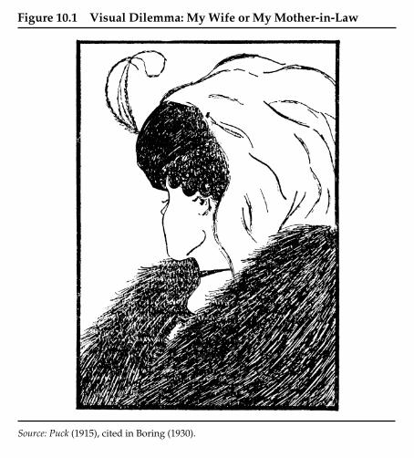
ordinary perception. The elegant dilemmas designed by philosophersand used by moral psychologists of the cognitive tradition are not unlikethese ambiguous pictures; they are designed to prevent the sort of swiftjudgment that occurs when we are judging others, instead elicitingdeliberative reasoning.

Another orienting distinction (though not a rigid one) between themoral dilemma situation and the moral reaction situation is one of per-spective. The dilemmas typically used in the moral dilemma situation(Kohlberg 1969; Colby, Kohlberg, and Kauffman 1987; Rest 1986),while sometimes third person at first glance (most famously the Heinzdilemma) are always designed to yield a fair amount of vacillation, and

Reason and Emotion in Moral Judgment 229

Source: Puck (1915), cited in Boring (1930).

Figure 10.1 Visual Dilemma: My Wife or My Mother-in-Law

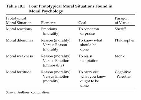
tially offensive behavior. The focus of morality is on how that behaviorwill be judged and what inference will be drawn about the perpetrator.This approach to morality is grounded in the social psychological tradi-tion of person perception and causal attribution, and has most recentlybeen defended in the social intuitionist model of moral judgment (Haidt2001). Moral judgments, in this approach, are “evaluations (good versusbad) of the actions or character of a person that are made with respect toa set of virtues held to be obligatory by a culture or subculture” (Haidt2001, 817). The social intuitionist model posits that moral judgments areprimarily based on moral intuitions, which are, in turn, defined as “thesudden appearance in consciousness of a moral judgment, including anaffective valence (good-bad, like-dislike), without any conscious aware-ness of having gone through steps of searching, weighing evidence, orinferring a conclusion” (Haidt 2001, 818). Like Justice Potter Stewart’sdefinition of obscenity, a moral act is judged to be right or wrongbecause you just “know it when you see it” (Woodward and Armstrong1979, 16). As mentioned above, this approach provides a valuable inte-gration of the traditional study of moral judgment and recent advancesin the study of emotion, implicit processes, and motivated cognition insocial psychology.

We refer to this class of situations as moral reactions to retain thebroader use of the term moral judgment, which is common in the literature.

Reason and Emotion in Moral Judgment 225

Table 10.1 Four Prototypical Moral Situations Found in Moral Psychology

Prototypical Paragon Moral Situation Elements Goal of Virtue

Moral reactions Emotions To condemn Sheriff(morality) or praise

Moral dilemmas Reason (morality) To know what PhilosopherVersus Reason should be (morality) done

Moral weakness Reason (morality) To resist MonkVersus Emotion temptation(immorality)

Moral fortitude Reason (morality) To carry out CognitiveVersus Emotion what you know Wrestler(morality) ought to be

done

Source: Authors’ compilation.


Source: Authors’ calculations.

Start and Quit Hours, Firm A

Clock Hour

Frac

tion

70

.1

.2

.3

.4

.5

9 11 13 15 17 19

Start Hour

Histogram

Histogram

Start and Quit Hours, Firm B

Quit Hour

Clock Hour

Frac

tion

70

.2

.4

.6

9 11 13 15 17 19

Figure 12.1 The Workday at Firms A and B

Affect and Cognition as a Source of Motivation 283

Figure 12.2 Daily Earnings


Firm A

Daily Earnings in Dollars

Frac

tion

500

.05

.1

.15

.2

.25

100 150 200 250

Firm B

Daily Earnings in Dollars

Frac

tion

500

.05

.1

.15

.2

.25

100 150 200 250

the 1 percent level, except for the coefficient for the first hour of the after-noon at Firm A, which is not significant.

Figure 12.3 shows that windfall gains in the morning have a statisti-cally significant impact on the effort profile in the afternoon, which iscontrary to the predictions of the standard cognitive model of laborsupply. On the other hand, the response of effort to the windfall gain isconsistent with the prediction that messengers attach affective signifi-cance to a daily earnings goal. As predicted by the alternative model oflabor supply, a messenger with a windfall gain works harder than othermessengers in the first part of the afternoon but less hard later in the day.Furthermore, the fact that the relative difference in effort increases over


Source: Authors’ calculations.Note: Mean revenues appr. $16/hour. Controls for (i) Messenger fixed effects, (ii) Firm*day fixed effects, (iii) Start hour. Standard errors adjusted for clustering on messenger.

–10

–8

–6

–4

–2

0

2

4

6

8

13 14 15 16 17 18Clock Hour

Cha

nge

in R

even

ues

per

Hou

r

Firm BFirm A

Figure 12.3 Effort over Time: The Impact of a $50 Increase inMorning Revenues (�/�2* s.e. of Estimate)

quit between five o’clock and six o’clock, and 35 percent quit betweensix o’clock and seven o’clock.

Figure 12.2 shows the distributions of daily earnings for messen-gers at Firm A and Firm B. Two features of these distributions are note-worthy: First, they are quite similar across firms. Second, daily earningsare highly variable. The standard deviation of daily earnings is $46.27 atFirm A and $50.29 at Firm B. Morning earnings, which are not shown,are also similarly variable, with a standard deviation of roughly $30.00at both firms.

There are several possible sources of the variation in messengers’earnings. We are particularly interested in the variation in morningearnings that represents windfall gains or luck. However, some of thevariation in earnings is certainly due to day-to-day fluctuations indemand for messenger services or differences in messenger characteris-tics. Therefore, to assess the importance of windfall gains for determin-ing a messenger’s earnings, we must first remove the variation due today and messenger effects. Table 12.2 shows an analysis of variance formorning earnings. The adjusted R-squared statistics indicate that dayand messenger effects explain a significant portion of the variation inmorning earnings at both firms. However, consistent with the predictionof an important role for luck in determining morning earnings, thereremains substantial unexplained variation. This variation is economi-cally meaningful to messengers, as shown by the fact that the standarddeviation of unexplained variance is equivalent to roughly 30 percent ofa messenger’s average morning earnings.

There are two important sources of randomness in daily earnings fora bicycle messengers. First, earnings vary with the characteristics of adelivery (that is, the service type, and the pick-up and drop-off zonesof the delivery) which are not necessarily correlated with the effortrequired to make the delivery. For example, two deliveries may involvethe same effort, but because one happens to cross the border of a pric-


Table 12.1 The Distribution of Hours on the Job

Firm A Firm B

6− 1.39 6− 0.947 3.30 7 1.458 8.73 8 4.559 24.39 9 20.3410 40.34 10 53.6311+ 21.85 11+ 19.00


ing zone in the city, it may generate significantly higher earnings.Messengers also talk about the importance of luck in generating a col-lection of deliveries that “line up,” allowing the messenger to deliver allpackages along a roughly linear path rather than having to make sig-nificant detours for each one. The second important source of random-ness comes from the fact that if one messenger gets a delivery due tofortunate timing in answering the dispatcher’s call, another messengeris prevented from getting the delivery.

Empirical Design

Our empirical strategy is to test for an impact of windfall gains in themorning on effort in the afternoon. In the standard model, within-daywindfall gains should have no impact on effort, because they are trivialrelative to lifetime and thus cannot change the marginal valuation ofincome. On the other hand, if workers attach affective significance to thelevel of their daily earnings, windfall gains could have an impact oneffort. The alternative model of effort that considers affect makes a dis-tinct prediction regarding the impact of a windfall gain in the morning:workers who had lucky mornings are predicted to work harder thanother messengers at the beginning of the afternoon because they are rel-atively closer to reaching their goals; the same workers are expected towork less hard than the others towards the end of the day because theyhave already surpassed their goals.

Our analysis focuses on the relationship between windfall gains inthe morning and effort in the afternoon. Although we could measurewindfall gains in terms of earnings, we instead use revenues, which area simple function of earnings (earnings/0.50); revenues have the advan-tage that they yield a direct interpretation in terms of benefits for the


Table 12.2 ANOVA for Morning Earnings.

Firm A Firm B

Adjusted R-squared

Date Fixed Effects .1238 .1000Date and Messenger Fixed Effects .3106 .5983

SD of Unexplained Variance 33.04 28.69(as percent of average morning earnings)

Observations 21,474 22,866



7

6

5

4

3

2

12 percentreal cut,

1 percentnominal cut

Anger Disappointment

2 percentreal cut,

1 percentnominal raise

4 percentreal cut,


4 percentreal cut,


3 percentreal raise,4 percent

nominal raise


nominal raise


nominal raise


nominal raise

Surprise Joy

Figure 13.1 Emotional Reactions to Different Wage Scenarios

results obtained in our study are thus consistent with Truman Bewley’sevidence. In a more recent study, Alexandre Mas (2005) examines theimpact of final-offer arbitrations between municipalities and police officerunions on subsequent law enforcement. The results he finds are strik-ing: in municipalities in which an arbitrator ruled against the police offi-cers, arrest rates tend to decrease over the subsequent year.9 Furthermore,larger “losses” relative to the level desired by the police officers lead toa larger drop in the arrest rate. On the other hand, larger “gains” do notsignificantly increase arrest rates. The results presented by AlexandreMas (2005) are thus consistent with a model in which individuals careabout outcomes relative to a reference outcome. While the results do notspeak to the point of whether nominal wage cuts lead to lower effort ofworkers, they do show that outcomes below a salient reference pointlead to lower effort.10

Overall, these results provide a strong rationale for why firms mightshy away from nominal wage cuts, especially when the desired nominalwage cut is small.

The Impact of Emotions on Wage Setting and Unemployment 305


6

5

4

3

2

12 percentreal cut,


Help out at workLook for another job

2 percentreal cut,


4 percentreal cut,


4 percentreal cut,


Figure 13.2 Changes in Job Loyalty in Different Job Scenarios

There were four different treatments in the first scenario. Table 13.1provides an overview over the different conditions. Each subject was ineither treatment A, B, C, or D. Subjects in treatment A in the first scenariowere in A′ in the second, and so on. Hence, all comparisons between A,B, C, and D (and their primed counterparts) measured between-subjectvariation. The others were identified by within-subject comparisons.6

Results

Figure 13.1 presents the emotional reactions to the different wagechanges, plotting the mean score for each emotion. The top panel offigure 13.1 shows scores for treatments A, B, C, and D. The bottom panelshows the scores for treatments A’, B’, C’, and D’. Comparing treatmentsA and B, which involved a 2 percent decrease in the real wage, to C andD, in which the real wage was cut by 4 percent, we see that a larger realwage cut leads to more anger and disappointment. However, comparingA to B, and C to D, we also see that the emotional reaction is consistentlystronger in cases in which there was a nominal wage cut compared tocases where there was not, holding the change in the real wage constant.Linear regression results, presented in table 13.2, tell a similar story. Thedependent variable for each regression is the corresponding emotionscore. As explanatory variables, we include dummy variables for eachof the possible real wage changes (from all scenarios), so that the effectof a nominal wage cut is identified by comparing A to B, and C to D.Because each subject participated in two scenarios, we adjusted the stan-dard errors to correct for possible correlation of the error term across


Table 13.1 The Treatment Conditions

Wage Changes in Scenario 1

Nominal Wage Change

1 Percent Cut 1 Percent Increase

Real Wage 2 percent decrease A BChange 4 percent decrease C D

Wage Changes in Scenario 2

Nominal Wage Change

4 Percent Increase 6 Percent Increase

Real Wage 3 percent increase A′ B′Change 1 percent increase C′ D′


observations for the same subject. Despite this conservative calculationof standard errors, we find a highly significant effect of a nominal wagecur: anger and disappointment are clearly higher, and joy is clearly lowerwhen a nominal wage cut is involved, holding the real wage change con-stant. Interestingly, the subjects also appeared more surprised by a realwage cut if it involved a nominal wage cut. Real wage changes clearlyalso matter for the evaluations, and the coefficients on the correspondingdummy variables indicate that these effects are quite large. For example,going from A to A’, or B to B’, we find large shifts in the evaluation ofthe wage scenario. Interestingly, when we compare A to C, and B to D,we find impacts that are much smaller, even though they entail the samedifference in the real wage change. The difference between the two com-parisons is that going from A to A′ is comparing a real wage loss to a realwage gain, while going from A to C is comparing a large loss to a smallloss (or to a small gain in the case of comparing A′ to C′). The differencein the results in these cases suggests the presence of strong loss aversionwith respect to the real wage.7

The design of the study also allows us to examine whether there issomething per se about a nominal frame that leads to a strong emotional


Table 13.2 Emotions Aroused by Different Scenarios of Wage Changes

Dependent Variable Anger Disappointment Surprise Joy

Nominal Wage Cut 0.7750 0.6041 1.2608 −0.8896(0.2126) (0.1799) (0.1798) (0.1559)

2 percent Real Wage −0.4132 −0.2537 0.0094 0.3120Cut (0.2118) (0.1781) (0.1791) (0.1532)

1 percent Real Wage −2.6542 −3.8096 0.7685 4.1165Raise (0.2003) (0.2000) (0.2210) (0.1791)

3 percent Real Wage −2.9165 −4.0913 1.3393 4.3463Raise (0.1867) (0.1809) (0.2055) (0.1794)

Constant 4.0513 5.3538 4.1359 2.0012(0.1810) (0.1633) (0.1660) (0.1450)

p-value that coefficient 0.912 0.976 0.059 0.63on nominal wage raiseis zero in augmentedregression

R-Squared 0.55 0.73 0.11 0.76N 554 554 554 554

Source: Authors’ calculations.Note: Dependent variables are measured on a seven-point scale to indicate whether theemotion describes their reaction to the proposed scenario. One indicates the lowest level of agreement, seven indicates the highest level of agreement. Robust standard errors,adjusted for clustering on individuals.

Evidence of Downward Nominal Wage Rigidity

This model predicts that nominal wage cuts occur less often than if work-ers were emotionless. To examine the relevance of this prediction in thefield, one needs data on individual wage observations. A mass pointat 0 percent wage changes, and a discontinuous drop in the density ofthe wage changes below zero, would be evidence of downward nominalwage rigidity (DNWR), as it might arise from behavioral forces.

One approach to testing for DNWR is thus to calculate a histogram ofwage changes, and assess the extent of a spike at nominal zero andasymmetry around zero. Studies that take this approach using data onthe U.S. labor market include those conducted by Kenneth McLaughlin(1994), David Card and Dean Hyslop (1996), Shulamit Kahn (1997), andDavid Lebow, Raven Saks, and Beth Anne Wilson (2003). The results indi-cate that some, but not much, nominal wage rigidity exists. Indeed, in anaverage year during the sample periods in these studies, about 20 per-cent of the workforce received nominal wage cuts, even though laborproductivity rose quite rapidly and inflation was quite high.


Table 13.3 Loyalty Towards Employer in Different Wage Change Scenarios

Willingness Will LookDependent Variable to Help Out for New Job

Nominal Wage Cut −0.3073 0.8665(0.1688) (0.1807)

2 percent Real Wage Cut 0.1525 −0.4876(0.1691) (0.1807)

1 percent Real Wage Raise 2.8469 −2.4079(0.1702) (0.1769)

3 percent Real Wage Raise 3.0545 −2.5477(0.1789) (0.1935)

Constant 2.4987 4.3491(0.1467) (0.1642)

p-value that coefficient on 0.764 0.477nominal wage raise is zeroin augmented regression

R-Squared 0.57 0.51N 554 554

Source: Authors’ calculations.Note: Dependent variables are measured on a seven-point scale to indicate whether theywould engage in the behavior described in response to the proposed scenario. One indicates the lowest level of agreement, seven indicates the highest level of agreement.Robust standard errors, adjusted for clustering on individuals.

figure 2.1 behavioral con sequencesitive and neg ... figures.pdfgration of the traditional study of...

Documents