Econometrics Review

Honors Exam PreparationApril 10th 2008

Disclaimer

• NOT an exhaustive list of material– Ec1126 – Focus on theory– Ec1123 – Focus on application

• Advised to review first 8 topics for 1123• No direction given for 1126• Refer to lecture notes and text book for

formulas and “formal” definitions

Suggested Study

1. Read the book /lecture outlines2. Review homework solutions3. Review previous exams4. Practice book exercises

Introduction

• Causality vs. Forecasting (Predicting)

• Data types– Cross Sectional – “Snap shot”– Panel – Multiple periods and entities– Time series – Multiple periods

Sampling

• Population data hard to analyze– Difficult or impossible to collect

• Collect sample from population– Easier to work with– Representative of population?

Sampling Distribution

• Population joint distribution F

• Sample for i=(1, …, n)(Yi1, …, Yim, Zi1, …, ZiJ)

• Random Sampling– Independent – Identically Distributed

Sampling Distribution

• It follows that sample is representative of population

• Law of large numbers• Sample mean converges in probability to population

mean as n approaches infiniti

• Central limit theory• Sample mean is asymptotically normally distributed

if random variable has a finite variance

Linear Regression

• Model: Yi = β0 + β1Xi + ui

• Terminology– Independent variable (Regressor)– Dependent variable– Intercept– Coefficient(s)– Error term

OLS• Ordinary Least Squares (OLS)

– min E(Yi - β0 - β1Xi)2 with choice variables β0, β1

• Assumption I: – (Yi - β0 - β1Xi) orthogonal to Xi

• Assumption II: – (XiYi) are iid from joint distribution

• Assumption III: – Large outliers unlikely

OLS• β1 = Cov(X,Y)/Var(X)

• By LLN Sxy and Sx are consistent estimators of population covariances above

• Coefficient estimates are consistent estimators of population coefficients– E(Y| 1, X) = β0 + β1Xi

OLS

• By LLN and CLT…

• Coefficient estimates are both consistent estimators of population coefficients and are asymptotically normally distributed

Hypothesis Tests & Confidence Intervals

• Hypotheses– Ho = Null – Ha = Alternative (False Null)

• Two-sided vs. One-sided Ha

• Confidence Intervals

Standard Errors

• Homoskedasticity vs. Heteroskedasticity – Estimators unbiased and asymptotically normal– Heteroskedastic variance of u|X not constant– Standard errors need to be corrected for

heteroskedasticity

• When is OLS BLUE?– I-III + Homoskedasticity

Omitted Variables• Does one regressor explain all of the variation in Y?

• Why does it matter? We’re looking at relationship between X1 and Y? Why do we care about X2?

• Omitted Variable Bias– Corr(X1 , X2) ≠ 0– Corr(Y , X2) ≠ 0– Sign of Bias = Sign of Corr(X1 , X2) * Sign of Corr(X2 , Y)

• Positive = Coefficient was previously biased upward• Negative = Coefficient was previously biased downward

Multiple Regression Model

• Model: Yi = β0 + β1X1i +…+ βkXki + ui

• Calculating OVB

– E(X2 | 1, X1) = π0 + π1X1i

– E(Y | 1, X1) = β0 + β1 E(X1i | 1, X1) + β2 E(X2i | 1, X1)

– E(Y | 1, X1) = β0 + β1X1i + β2 (π0 + π1X1i )

– E(Y | 1, X1) = (β0 + β2 π0) + (β1+β2 π1) X1i

Multiple Regressors

• Assumptions I-III

• Homoskedasticity vs. Heteroskedasticity

• Perfect multicollinearity– Assumption IV of OLS

Hypothesis tests & Confidence Intervals

• Confidence Interval calculation for single coefficient no different in a multiple regressor model

• Joint Hypothesis– F-test– Restrictions (q)

• Test Joint Hypotheses– Ho: ß1=ß2=0– Ha: ß1=0 and/or ß2=0– q=2

Nonlinear models

• Polynomial Model– Yi = β0 + β1X1i + β2X2

1i + … + ui

• Logarithmic Model– Linear-log Yi = β0 + β1ln(X1i) + ui

– Log-linear ln(Yi) = β0 + β1X1i + ui

– Log-log ln(Yi) = β0 + β 1ln(X1i) + ui

• Interaction Model– Yi = β0 + β1X1i + β2X1i Di

Nonlinear models

• Effect of a change in X depends on more than just β1

• Test Non-linearity – Ho: β2 =… βk =0– Ha: β2 ≠… and/or … βk ≠ 0

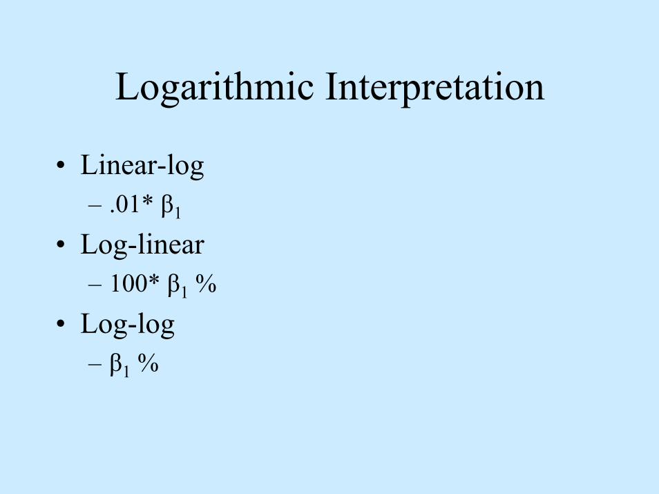
Logarithmic Interpretation

• Linear-log– .01* β1

• Log-linear– 100* β1 %

• Log-log– β1 %

Interaction Models

• Dummy variables (Binary variables)• Types & Interpretation

– Binary * Binary– Binary * Continuous

• Different Intercept• Different Intercept and Slope• Same Intercept and Different Slope

Ec1123

STOP!

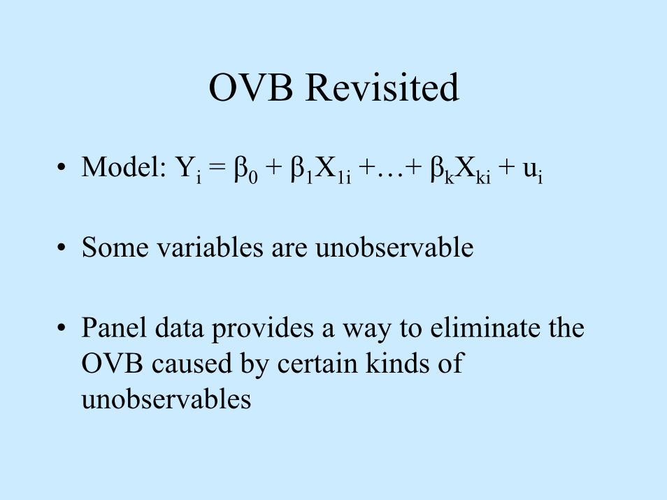
OVB Revisited

• Model: Yi = β0 + β1X1i +…+ βkXki + ui

• Some variables are unobservable

• Panel data provides a way to eliminate the OVB caused by certain kinds of unobservables

Panel Data

• Structural Regression FunctionE(Yt | 1, Zt,.., ZT)= θ0 + θ1Zt +…+ θ2W + θ3A

• Where:– Zt is predictor (varies by time)– W and A are time-invariant variables– Assume A is not observed so there is no sample

counterpart

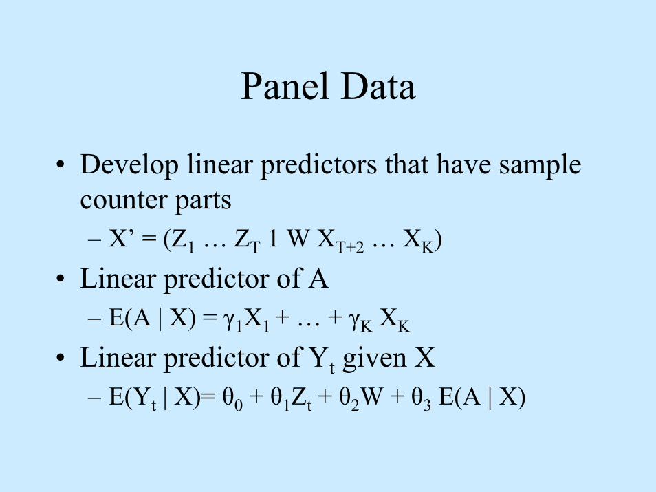
Panel Data

• Develop linear predictors that have sample counter parts– X’ = (Z1 … ZT 1 W XT+2 … XK)

• Linear predictor of A– E(A | X) = γ1X1 + … + γK XK

• Linear predictor of Yt given X– E(Yt | X)= θ0 + θ1Zt + θ2W + θ3 E(A | X)

System of Linear Predictors

• For T=2– E(Y1 | X) = (θ1 + θ3γ1)Z1 + θ3 γ2Z2 + R – E(Y2 | X) = θ3γ1Z1 + (θ1 + θ3γ2)Z2 + R– R is a placeholder

• Exploit the common coefficients– (θ1 + θ3γ1) - θ3γ1 = θ1

• However there remain unidentified coeffs.

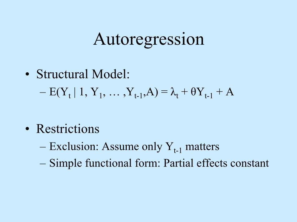
Autoregression

• Structural Model:– E(Yt | 1, Y1, … ,Yt-1,A) = λt + θYt-1 + A

• Restrictions– Exclusion: Assume only Yt-1 matters– Simple functional form: Partial effects constant

Setup

• Start with Y1 since there is no Y0– E(Y1| 1, A) = δ0 + δ1A

• Structural Model:– Y1 = δ0 + δ1A + V– Yt = λt + θYt-1 + A + Ut

Estimating θ

• Substitute for Y1 in equation for Y2– Y2 = λ2 + θ(δ0 + δ1A + V)+ A + U2

• Recursively substitute for t+1

• θ can be expressed as a function of Yt and Ys covariances

Reminders

• Not intended to be an exhaustive list

• Reference lecture notes and book for formulas or formal definitions

• Practice old homework and exam problems