file name: supplementary information description
TRANSCRIPT

File name: Supplementary Information Description: Supplementary figures, supplementary tables, supplementary notes and supplementary references.

1/44
Supplementary Note: Model and Algorithm Details for 1
DPR 2
The latent Dirichlet process regression model 3
We consider the following multiple linear regression model 4
2~ (0 σ )e nN= + + , , ,y W X Iα β ε ε (1) 5
where y is an n-vector of phenotypes measured on n individuals; W is an n by c matrix of 6
covariates including a column of 1s for the intercept term; α is a c-vector of coefficients; 7
X is an n by p matrix of genotypes; β is the corresponding p-vector of effect sizes; ε is 8
an n-vector of residual errors where each element is assumed to be independently and 9
identically distributed from a normal distribution with variance 2σe . Note that we use β 10
here instead of β as in the main text for reasons that will become clear shortly. 11
As explained in the main text, we assign a normal prior N(0, 2 2σ σe ) on each element of 12
β , and we further assign a Dirichlet process prior on the variance parameter 2σ . (Note 13
that different from the main text, we also scale the variance with the error variance 2σe to 14
simply the algorithm.) Integrating out 2σ induces a Dirichlet process normal mixture 15
prior on iβ 16
2 2 2
1
1
1
~ (0 (σ σ )σ ),
= (1 ) ~ Beta(1 λ),
i k k b ek
k
k k l kl
Nβ π
π ν ν ν
∞
=
−
=
, +
− , ,
∏
(2) 17
where 2 2σ σk b+ (scaled by 2σe ) is the variance for each normal component. Again, to 18
simply the algorithm, different from the main text, we add a common variance 2σb to 19
each variance component and we set 2σk = 0 when k = 1. We refer to the above model 20
based on equations (1) and (2) as the latent Dirichlet Process Regression (DPR) model. 21
For the hyper-parameters α, 2σk , 2σb , 2σe , and λ in the model, we consider the following 22
priors 23

2/44
2 2 2
20 0
20 0
20 0
0λ 0λ
~ (0 ),
σ ~ inverse-gamma ( ),
σ ~ inverse-gamma ( ),
σ ~ inverse-gamma ( ),
λ ~ gamma( ),
j e w w
k k k
b b b
e e e
N
a b
a b
a b
a b
α σ σ σ, → ∞,
,
,
,,
(3) 24
where we set 0ka , 0kb , 0ba , 0bb , 0ea , and 0eb in the inverse gamma distributions to be 0.1; 25
we set 0λa and 0λb in the gamma distribution to be 1 and 0.1; and we use a limiting 26
normal prior for each αj with the normal variance goes to infinity, since generally there is 27
enough information in the likelihood to overwhelm any reasonable prior assumption for 28
these parameters. 29
To improve mixing, following1, we group the effect sizes that correspond to the first 30
normal component with the smallest variance 2σb in equation (2) into a random effects 31
term u: 32
2 2~ (0, σ σ )b eN= ,u Xb K (4) 33
where /T p=K XX is the genetic relatedness matrix (GRM)1,2 computed using centered 34
SNPs. Note that the GRM is typically positive semi-definite with one eigen-value being 35
zero due to genotype centering. We do not need to deal with the zero eigenvalue because 36
our algorithms do not involve the inverse of GRM. This way, the model in equation (1) 37
becomes 38
2~ (0 σ )e nN= + + + , , ,y W X u Iα β ε ε (5) 39
explaining our use of β in equation (1). In our notation, β = β + b. The corresponding 40
prior on each element of b is 41
2 2~ (0 σ σ / )i b eb N p, , (6) 42
and the corresponding prior on each element of β is 43
2 2 21
2
~ (0 0 σ ) (0 σ σ )i e k k ek
N Nβ π π∞
=
, × + , . (7) 44
We will develop algorithms for fitting the equivalent model defined in equation (5) in the 45
following text. With the fitting algorithm, we can obtain the posterior mean of β as the 46
3/44
sum of the posterior mean of β and the posterior mean of b. We use the posterior mean of 47
β to compute prediction errors. 48
Difference between DPR and BayesR 49
Before we proceed further, it is useful to clarify the difference between DPR and the 50
previously proposed method BayesR3. While our method is motivated in part by BayesR, 51
DPR is different from BayesR in five important areas. First, BayesR is a sparse model 52
while DPR is a non-sparse model: BayesR assumes that most SNPs have zero effects 53
while DPR assumes that all SNPs have non-zero effects. As a result, BayesR and DPR 54
are expected to perform differently in sparse vs non-sparse settings. Second, BayesR 55
fixes the ratio between the variance parameters from the three non-zero components to be 56
0.01:0.1:1. In contrast, DPR estimates the variance of all non-zero components from the 57
data at hand. Inferring parameters from the data instead of fixing them to pre-set values is 58
expected to improve prediction performance. Third, BayesR uses a mixture of three 59
normal distributions for the non-zero component, while DPR uses infinitely many normal 60
distributions a priori. Using three normals can sometimes fail to capture the complicated 61
effect size distributions encountered in a range of genetic architectures, as is evident in 62
simulations presented in the main text. Fourth, importantly, it is not straightforward to 63
extend BayesR to accommodate a larger number of normal components. Consequently, 64
while the BayesR software allows users to specify an arbitrary number of components, in 65
those analyses, BayesR also requires users to provide the variance component estimates 66
for these components. It is far from trivial to figure out how one should obtain these 67
variance component estimates for BayesR. In contrast, DPR provides a principled way to 68
extend the simple normal model to accommodate a much larger number of normal 69
components, ensuring robust prediction performance across a range of settings. Fifth, as 70
we will show below, we fix the number of normal components in DPR in practice due to 71
computational reasons. As has been previously shown in other settings11,12, using a small 72
number of components to approximate the Dirichlet process can undermine its 73
performance. Therefore, we do want to acknowledge that the results we present in the 74
main text are likely conservative estimates of DPR’s performance. Better approximations 75
to the Dirichlet process may improve DPR’s prediction performance further. 76
4/44
MCMC sampling 77
Here, we describe our Markov Chain Monte Carlo (MCMC) sampling algorithm to 78
obtain the posterior samples from DPR. To facilitate MCMC, for each SNP i, we assign a 79
vector of indicator variables {0,1}ikγ ∈ to indicate which normal component iβ comes 80
from. To improve convergence, we integrate out u in model (5) and then perform Gibbs 81
sampling by using the conditional distributions for each parameter in turn. Specifically, 82
let 2 2 2( σ σ λ σ )b k k ik eν γ= , , , , , , ,θ α β includes all unknown parameters in model (5), our 83
joint log marginal posterior after integrating out u is 84
2 2 2 2
2 20 0 0 0
20 0 0λ 0λ
2 12
2
log ( | ) log ( σ σ ) log ( σ σ )
log ( ) log ( λ) log (σ ) log (σ )
log (σ ) log (λ )
1 1log | σ | ( ) ( )
2 2σ
1( log(
2
b e k e
k k k k k e e e
b b b
Te
e
iki k
p p p
p p p a b p a b
p a b p a b
C
ν ν
γ
−
∞
=
= | , , , + | , ,
+ | + | + | , + | ,
+ | , + | ,
= − − − − − −
+ −
y y β
H y W Xβ H y W Xβ
βθ α γ
γ
α α
22 2
2 2
1
1
2 2 2 20 0 0 0
2 20 0 0λ 0λ
1σ ) log(σ ) )
2 2σ σ
(log( ) log(1 )) ((λ 1) log(1 ) + log(λ))
( 1) log(σ ) σ ( 1) log(σ ) σ
( 1) log(σ ) σ ( 1) log(λ) λ,
ike k
k e
k
ik k l ki k l k
k k k k e e e ek k
b b b b
a b a b
a b a b
β
γ ν ν ν∞ − ∞
=
∞ ∞− −
−
− −
+ + − + − −
− + − − + −
− + − + − −
(8) 85
where 2σn b= +H I K and C is a normalizing constant. To simplify notation, we will 86
ignore all constant terms from now on. Based on the joint posterior, we can derive the 87
conditional posterior distribution for each parameter in turn. When we derive these 88
conditional distributions, we will also ignore the other parameters which these 89
distributions are conditional on to simplify the presentation. 90
Sampling α j 91
First, for jα we have 92
2 1
2 2 1σlog ( | .) σ ( ) .
2
Te j j T
j j e j m m jm j
p α α α α− −
− −
≠
= − + − −w H w
w H y w Xβ (9) 93
Therefore, the conditional distribution for sampling jα is 2( | .) ( ),j j jp N m sα = , where 94
5/44
1
1
22
1
( )
σ
Tj m m
m jj T
j j
ej T
j j
m
s
α−
≠−
−
− −= ,
= .
w H y w Xβ
w H w
w H w
(10) 95
Sampling β ik and γ ik 96
For ikβ and ikγ , we have 97
2 12 2 1
12 2 2 2 2
1
σlog ( | .) σ ( )
2
1 1 1( log(σ ) log(σ ) σ σ ) (log( ) log(1 )).
2 2 2
TTe i i
ik ik i e i m m im i
k
ik e k e k ik ik k ll
p β γ β β β
γ β γ ν ν
− −− −
≠
−− −
=
, = − + − −
+ − − − + + −
x H xx H y W xα
(11) 98
Therefore, the conditional distributions for sampling ikβ and ikγ are 99
12 21
2
/2 log( ) log(σ ) log(σ ) log( ) log(1 )
( 1,.) ( )
( 1| .) ,k
ik ik ik e k k ll
ik ik ik ik
m s s
ik ik
p N m s
p eν ν
β γ
γ π−
=+ − − + + −
| = = , ,
= = ∝ (12) 100
where 101
1
1 2
22
1 2
( )
σ
σ
σ
Ti m m
m iik T
i i k
eik T
i i k
m
s
β−
≠− −
− −
− −= ,
+
= .+
x H y W x
x H x
x H x
α
(13) 102
Sampling νk 103
For νk, we have 104
1
log ( | .) log( ) log(1 ) (λ 1) log(1 ).k ik k il k ki i l k
p ν γ ν γ ν ν∞
= +
= + − + − − (14) 105
Therefore, the conditional distribution for sampling νk is ( | .) Beta( λ )k k kp ν κ= , , where 106
1
1,
λ λ.
k iki
k ili l k
κ γ
γ∞
= +
= +
= +
(15) 107
6/44
Sampling 2σ k 108
For 2σ k , we have 109
2 2
2 2 20 0
σlog (σ | .) ( 1) log(σ ) ( )σ .
2 2ik ik ik ei i
k k k k kp a bγ γ β −
−= − + + − + (16) 110
Therefore, the conditional distribution for sampling 2σ k is 111
2(σ | .) inverse-gamma( )k k kp a b= , , where 112
0
202
1,
21
.2σ
k ik ki
k ik ik kie
a a
b b
γ
γ β
= +
= +
(17) 113
Sampling λ 114
For λ, we have 115
0λ 0λlog (λ|.) λ( log(1 ) ) + log(λ)( 1 ).k kk k
p b aν∞ ∞
= − − + (18) 116
Therefore, the conditional distribution for sampling λ is λ λ(λ|.) gamma( ),p a b= , where 117
λ 0λ
λ 0λ
1 ,
log(1 ).
kk
kk
a a
b b ν
∞
∞
= +
= − −
(19) 118
Sampling 2eσ 119
For 2σe , we have 120
2 2 20
2
2 2 20
1log (σ | .) (( ) / 2 1) log(σ ) SSR σ
2
1( σ 2 )σ .
2
e ik e e ei k
ik ik k e ei k
p n a
b
γ
γ β
−
=
− −
= − + + + − ×
− +
(20) 121
Therefore, the conditional distribution for sampling 2σe is 2(σ | .)ep = inverse-gamma(ae, be) 122
where 123
7/44
02
2 20
2
1
/ 2 / 2 ,
1(SSR / σ 2 ),
2
SSR ( ) ( ).
e ik ei k
e ik ik k ei k
T
a n a
b b
γ
γ β
=
=
−
= + +
= + +
= − − − −
y W X H y W Xα β α β
(21) 124
Sampling 2bσ 125
For 2bσ , we have 126
2 1
2
2 20 0
1 1log (σ | .) log | | ( ) ( )
2 2σ
( 1) log(σ ) σ ,
Tb
e
b b b b
p
a b
−
−
= − − − − − −
− + −
H y W X H y W Xα β α β (22) 127
which is in an unknown distributional form. Nevertheless, it is straightforward to sample 128
from this univariate distribution using reject sampling, importance sampling or other 129
standard methods4. Here, we sample 2σb based on re-parameterization of 2σb following1,5. 130
Specifically, we define a new parameter (h2)2,6,7 131
2
22
σ
σ 1b
b
h =+
, (23) 132
which is bounded between 0 and 1. The log-posterior conditional distribution for h2 is 133
2 2 2 2log ( | .) log (σ ( ) | .) 2 log(1 )bp h p h h= − − , (24) 134
where 2 2(σ ( ) | .)bp h is the posterior conditional distribution given in (22) with 135
2 2σ ( )b h = 2 2/ (1 )h h− . We then use the Metropolis-Hastings algorithm to generate 136
posterior samples for h2. In particular, we use the independent random walk algorithm for 137
h2 with a Beta(2,8) distribution as the proposal distribution. With each sampled value of 138
h2, we can obtain a sampled value of 2σb = 2 2/ (1 )h h− . 139
Sampling b 140
Finally, because of the relationship between u and b in equation (4), we can obtain 141
the posterior conditional distribution for b as 142
2
1 2 2 1 2 2 1σ( | .) MVN ( ( ), σ σ ( σ ))T Tb
p b e p bp p pp
− − − −= − − −b X H y W X I X H Xα β , (25) 143
8/44
where MVNp(μ, Σ) is a p-dimensional multivariate normal distribution with mean μ and 144
variance-covariance Σ. To reduce variance, we use the Rao-Blackwellised approximation 145
to compute the mean of b at the end of the MCMC sampling, with 146
2 ( ) ( ) 1 ( ) ( )
1
1 1ˆ (σ ) ( ) ( )L
Tbp L
−
=
= − −b X H y W X
α β . (26) 147
where L is the total iterations of MCMC after burn in, denotes the posterior samples. 148
These b̂ are added back to the posterior mean of β to yield the posterior mean of β . 149
Efficient computation 150
We apply the algebra innovations recently developed for linear mixed models1,8,9 to 151
improve computational efficiency. Specifically, at the beginning of MCMC, we perform 152
an eigen decomposition of K = UDUT, where U is the matrix of eigenvectors and D is a 153
diagonal matrix of eigenvalues1,8,9. Then we transform phenotype, genotypes and 154
covariates as UTy, UTX, and UTW. Afterwards, the likelihood conditional on the 155
transformed variables become independent, thus alleviating much of the computational 156
burden associated with the complex covariance structure resulted from the random 157
effects u. 158
The per-iteration computational cost of the above naive MCMC algorithm, after 159
applying the linear mixed model algebra innovations, scales linearly both with the 160
number of individuals and with the number of SNPs. Such computational cost can still be 161
burdensome when we have millions of SNPs. To improve computation efficiency further, 162
we develop a new, prioritized sampling strategy based on the recently developed random 163
scan Gibbs sampler10,11. Specifically, we take advantage of the fact that for any complex 164
traits, most SNPs have small effects (or are non-causal) while only a small proportion of 165
SNPs have large effects (or are causal). The likely causal SNPs are important for 166
phenotype prediction and their effect sizes need to be estimated accurately. In contrast, 167
the likely non-causal SNPs often do not influence prediction performance much and their 168
effect sizes individually do not require accurate estimation. Therefore, it is desirable to 169
spend a large amount of computational resource on sampling likely causal SNPs to 170
obtain accurate effect size estimates, while assigning a small amount of resource on 171
sampling likely non-causal SNPs. Certainly, the above arguments are all conditional on a 172
9/44
fixed number of SNPs (i.e. spend extra computational resource on updating a fixed 173
number of likely causal SNPs vs updating a fixed number of likely non-causal SNPs). To 174
perform such prioritized sampling, we first obtain the top M marginally significant SNPs 175
using LMM with the GEMMA algorithm. We treat these M selected SNPs as likely 176
causal SNPs and update their effect sizes in each MCMC iteration. We then treat the 177
unselected SNPs as likely non-causal SNPs and update their effect sizes once every T 178
iterations. We set M = 500 and T = 10 (both are set to allow fast computation since the 179
association signals are relatively strong in these two data) for the cattle and maize data, 180
M = 105 and T = 2 (the two are set differently as the signals are relatively weak in this 181
data) for the FHS data in the present study; for the GEUVADIS data we performed a full 182
MCMC sampling as the small sample size there allows for efficient computation. Note 183
that the choice M and T theoretically does not affect the stationary distribution, and we 184
recommend exploring a few values of M and T in practice to achieve a balance between 185
speed and accuracy. By prioritizing the computation resource on sampling the likely 186
causal SNPs, our computational algorithm results in a dramatic reduction in 187
computational cost, while yielding the same stationary distribution and maintaining the 188
predictive performance of DPR. As an example, for the three traits MFP, MY and SCS in 189
the cattle data, our naive MCMC takes approximately 25 hours to run 50,000 MCMC 190
iterations. In contrast, our prioritized sampling algorithm reduces the computational cost 191
down to approximately 5 hours, resulting in a five-fold speed improvement. The 192
prediction performance of the prioritized sampling algorithm remains comparable with 193
that of the naive MCMC: the resulting R2 and MSE from the two algorithms were almost 194
identical, with a correlation above 0.995 across 20 data splitting replicates. Note that the 195
prioritizing sampling strategy we employ in DPR differs from the sample strategy used in 196
BayesR3, where a different set of M SNPs are used every T iteration. Indeed, our 197
sampling strategy is still guaranteed to reach the same stationary distribution given a 198
large number of iterations, regardless which set of M SNPs or which set of M and T 199
values we choose to perform prioritized sampling. 200
Finally, we follow the truncated stick-breaking approximation approach of Blei and 201
Jordan12,13 and approximate the infinite normal mixture by a truncated normal mixture 202
with K normal components. To ensure that kπ is well defined under the truncated 203
10/44
approximation (i.e. 1
1K
kkπ
== ), we set 1kv = , 1 0kv− = for k>K12,14,15. With the 204
truncated Dirichlet process approximation, we can draw posteriors via a simple Gibbs 205
sampler, thus alleviating much of the computational burden associated with sampling the 206
full Dirichlet process conditionally through the Chinese restaurant process. Because 207
different truncated normal mixture approximations may result in different accuracy, we 208
treat K as a parameter and use the deviance information criterion (DIC)15-17 to select the 209
optimal K automatically. To do so, we first perform MCMC sampling on a grid of K 210
values from 2 to 10. For each K, we compute DIC using a small number of MCMC 211
iterations (5,000). We select the optimal DPR model with the smallest DIC. We then run 212
a large number of MCMC iterations (50,000) with the optimal DPR model. This strategy 213
makes the selection of K in our DPR adaptive, while keeping computational cost in check. 214
Note that this selection strategy may lead to local optimal and consequently hinders the 215
performance of our method. Alternative and better strategies may improve DPR’s 216
prediction performance further. For the final 50,000 MCMC iterations, we discarded the 217
first 10,000 as burn in and kept the remaining 40,000 for parameter estimation. We did 218
not thin the MCMC chain18, which may help improve prediction performance further. 219
Finally, we also provided trace-plots for the log posterior likelihood of our model in all 220
real data analyses following the recommendation in15,19. These trace-plots serve as a 221
summary assessment of parameter convergence. 222
Mean Field Variational Inference for DPR 223
Despite the many algorithm innovations we use, the resulting MCMC algorithm is 224
still computationally heavy. Therefore, we develop an alternative, much faster, algorithm 225
based on variational Bayesian approximation12,20-23. Variational Bayesian approximation 226
attempts to approximate the joint posterior distribution by a variational distribution, 227
( )q θ = ( )jjq θ∏ , that assumes posterior independence among parameters θj. To do so, 228
we minimize the Kullback-Leibler (KL) divergence between ( )p | yθ and ( )q θ 229
( )
( ) ( )
( )KL( ( ) ( )) (log ),
( )
(log ( )) (log ( )) log ( ).
q
q q
qq p E
p
E q E p p
| | =|
= − , +
yy
y y
θ
θ θ
θθ θθ
θ θ (27) 230
11/44
Because the marginal probability log ( )p y does not depend on the variational 231
distribution, minimizing the KL divergence is equivalent to maximizing the evidence 232
lower bound (ELBO) 233
( ) ( )(log ( )) (log ( ))q qE p E q, − .yθ θθ θ (28) 234
To obtain the variational approximation, we can use the gradient ascent algorithm to 235
maximize the above quantity with respect to each jθ in turn. For each jθ , we set the 236
following derivative 237
( ) ( )
( )
( )
(log ( )) (log ( ))
( )
( ( ) (log ( )) ( ) log ( ) )
( )
(log ( )) log ( ) 1
j
j
q q
j
j q j j j j
j
q j
E p E q
q
q E p d q q d
q
E p q
θ
θ
θ
θ θ θ θ θθ
θ
−
−
∂ , −∂
∂ , −=
∂
= , − −
y
y
y
θ θθ θ
θ
θ
(29) 238
to zero. Because ( )p , yθ does not contain any parameter in ( )jq θ , this leads to an update 239
for each jθ in the following form 240
( ) ( )(log ( )) (log ( ))( ) .q q j jj j
E p E p
jq e eθ θθ θ θθ − − −, | ,∝ ∝
y y (30) 241
Inference based on the above factorized form of the variational distribution is commonly 242
known as the mean field variational Bayesian approximation inference20,21,23-25. 243
We apply the mean field variational Bayesian approximation to DPR. Because 244
computing ELBO is difficult for non-analytic variational distributions26,27, we cannot 245
integrate out u from model (5) as we do for MCMC. Instead, we keep u. We also denote 246
g = UTu. Our joint log posterior is 247
12/44
2 2 2 2
2 20 0 0 0
20 0 0λ 0λ
22
2
log ( ) log ( ) log ( σ σ ) log ( σ σ )
log ( ) log ( λ) log (σ ) log (σ )
log (σ ) log (λ )
1log(σ ) ( ) ( )
2 2σ
k e b e
k k k k k e e e
b b b
Te
e
i k
p p p p
p p p a b p a b
p a b p a b
nC
ν ν
γ∞
=
, = | , , + | , , + | ,
+ | + | + | , + | ,
+ | , + | ,
= − − − − − − − −
+
y y u u
y W X u y W X u
β γγ
θ α β
α β α β
22 2
2 2
2 2 2 2 1
1
1 1
2 2 20 0 0 0
1 1( log(σ ) log(σ ) )
2 2 2σ σ
1 1log(σ ) log(σ ) log | | (σ σ )
2 2 2 2
(log( ) log(1 )) ((λ 1) log(1 )+ log(λ))
( 1) log(σ ) σ ( 1) log(σ )
ikik e k
k e
Te b e b
k
ik k l ki k l k
k k k k e e ek k
n n
a b a b
β
γ ν ν ν
−
∞ − ∞
= =
∞ ∞−
− − −
− − − −
+ + − + − −
− + − − + −
K u K u
2
2 20 0 0λ 0λ
σ
( 1) log(σ ) σ ( 1) log(λ) λ,
e
b b b ba b a b
−
−− + − + − − (31) 248
where again C is a normalizing constant. We will ignore the constant terms in the 249
following updates. 250
We follow the truncated stick-breaking approximation approach of Blei and Jordan12 251
and use a finite mixture with a fixed number of normal components, K, as an 252
approximation to the posterior distribution. The parameter K here is considered as a 253
variational parameter and we choose K by optimizing ELBO. Note again that although 254
we use a finite mixture as an approximation to the posterior distribution, our likelihood 255
still consists of a mixture of infinitely many normal distributions12. To choose K, we 256
perform variational inference with DPR on different K values ranging from 2 to 10. 257
Following12, we then choose the optimal DPR model with the largest ELBO and we 258
present results based on the optimal DPR. 259
Variational distribution for α j 260
First, for jα , we have 261
22
2
(σ )log ( )
2
(σ ) ( ( ) ( ) ( ) .
Te j j
j j
Te j m m j
m j
Eq
E E E E
α α
α α
−
−
≠
= −
+ − − −
w w
w y w X u)β (32) 262
13/44
Therefore, the variation distribution for jα is 2( ) ( ),j j jq N m sα = , where 263
2 1
2
( ( ) ( ) ( ))
(σ )
Tj m m
m jj T
j j
ej T
j j
E E E
m
Es
α≠
− −
− − −= ,
= .
w y w X u
w w
w w
β
(33) 264
Variational distributions for βik and γ ik 265
For ikβ and ikγ , we have 266
22
2
2 2 2 2 2
1
1
(σ )log ( ) ( )
2
(σ ) ( ( ) ( ) ( ))
1 1 1( log (σ ) log (σ ) (σ ) (σ ) )2 2 2
(log ( ) log (1 )).
Te i i
ik ik i
Te i m m i
m i
ik e k k e ik
k
ik k ll
Eq E
E E E E
E E E E
E E
β γ β
β β
γ β
γ ν ν
−
−
≠
− −
−
=
, = −
+ − − −
+ − − −
+ + −
x x
x y W x uα
(34) 267
A natural update form for ( )ik ikq β γ, is thus 268
12 21
2
/ 2 log( ) (log(σ )) (log(σ )) (log( )) (log(1 ))
( 1) ( )
( 1) ,k
ik ik ik e k k ll
ik ik ik ik
m s s E E E E
ik ik
q N m s
q eν ν
β γ
γ ϕ−
=+ − − + + −
| = = , ,
= = ∝ (35) 269
where 270
2
2 12
2
( ( ) ( ) ( ))
(σ )
(σ )
(σ )
Ti m m
m iik T
i i k
eik T
i i k
E E Em
E
Es
E
β≠
−
− −
−
− − −= ,
+
= .+
x y W x u
x x
x x
α
(36) 271
Variational distribution for ν 272
For ν, we have 273
1
log ( ) ( ) log( ) ( ) log(1 ) ( (λ) 1) log(1 ).k ik k il k ki i l k
q E E Eν γ ν γ ν ν∞
= +
= + − + − − (37) 274
Thus ( ) Beta( λ )k k kq ν κ= , , where 275
14/44
1
( ) 1,
λ ( ) (λ).
k iki
k ili l k
E
E E
κ γ
γ∞
= +
= +
= +
(38) 276
Variational distribution for 2kσ 277
For 2σ k , we have 278
2 2
2 2 20 0
( ) ( ) (σ )log (σ ) ( 1) log(σ ) ( )σ .
2 2ik ik ik ei i
k k k k k
E E Eq a b
γ γ β −−= − + + − +
(39) 279
Thus 2(σ ) inverse-gamma( ),k k kq a b= , where 280
0
2 20
1( ) ,
21
( ) (σ ) .2
k ik ki
k ik ik e ki
a E a
b E E b
γ
γ β −
= +
= +
(40) 281
Variational distribution for λ 282
For λ, we have 283
0λ 0λlog (λ) λ( log (1 ) )+ log(λ)( 1 ).k kk k
q E b aν∞ ∞
= − − + (41) 284
Thus λ λ(λ) gamma( ),q a b= , where 285
λ 0λ
λ 0λ
1 ,
log (1 ).
kk
kk
a a
b b E ν
∞
∞
= +
= − −
(42) 286
Variational distribution for g 287
For g, we have 288
2
2 2 1
1log ( ) ( ( ) ( ) ) ( ( ) ( ) )
2σ
1(σ σ ) .
2
T T T T T T T
e
Te b
q E E E E
−
= − − − − − − −
−
g U y U W U X g U y U W U X g
g D g
α β α β(43) 289
Thus ( ) MVN ( , ),nq =g μ Σ where 290
15/44
2 1 1
2 1 1 2 1
( (σ ) ) ( ( ) ( )),
( (σ ) ) (σ ) .
T T Tb n
b n e
E E E
E E
− − −
− − − − −
= + − −
= +
D I U y U W U X
D I
μ α β
Σ (44) 291
Here, the covariance matrix is diagonal, which facilitates computation. As in MCMC, we 292
use the relationship in equation (4) to obtain the mean of b at the end of the algorithm. 293
The estimated mean of b is added back to the mean of β to obtain a mean estimate for β . 294
Variational distribution for 2bσ 295
For 2bσ , we have 296
2 2 2 2 2 2 20 0
1log (σ ) log(σ ) σ ( ) / ( σ ) ( 1) log(σ ) σ ,
2 2b b b i i e b b b bi
nq E g E d a b− −= − − − + − (45) 297
where di is the ith diagonal element of D. Thus 2(σ ) inverse-gamma( ),b b bq a b= , where 298
0
2 1 20
,21
( ) ( σ ) .2
b b
b i i e bi
na a
b E g E d b− −
= +
= + (46) 299
Variational distribution for 2eσ 300
Finally, for 2eσ , we have 301
2 2 20
2
2 2 2 2 20
1log (σ ) ( ( ) / 2 1) log(σ ) σ
2
1( ( ) (σ ) ( ) / ( σ ) 2 )σ .
2
e ik e e ei k
ik ik k i i b e ei k i
q n E a A
E E E g E d b
γ
γ β
−
=
− −
= − + + + − ×
− + +
(47) 302
Thus 2(σ ) inverse-gamma( ),e e eq a b= , where 303
02
2 2 2 2 10
2
2 2 2 2
( ) / 2 ,
1( ( ) (σ ) ( ) (σ ) 2 ),
2
( ( ) ( ) ( )) ( ( ) ( ) ( ))
( ( )( ) ( ( ) ) ),
e ik ei k
e ik ik k i b i ei k i
T T T T T T T
T Tj j j ii i i ik ik ik ik ik
j i i k k
a n E a
b A E E E g E d b
A E E E E E E
s E m s E m
γ
γ β
γ γ
=
− − −
=
= + +
= + + +
= − − − − − −+ + + + −
U y U W U X g U y U W U X g
w w x x
α β α βΣ
(48) 304
where iiΣ is the ith diagonal element of Σ given in (44). 305

16/44
To evaluate all the above expectations, we need 306
2
( )
( )
2 2 2( )
( )
2 2 2( )
( )
( )
(
(log( )) ( ) ( ),
(log(1 )) ( ) ( ),
( ) ( ),
( ) ,
( ) ,
( ) ,
( ) ,
1(logσ ) (log( ) ( )),
2
k
k
i i
i i
j
j
k
q k k k k
q k k k k
i i ik ik ikqk
i ik ikqk
q j j j
q j j
k k kq
q
E
E
E m s
E m
E m s
E m
E
E b a
E
ν
ν
γ β
γ β
α
α
σ
ν κ κ λν λ κ λ
γ β ϕ
β ϕ
α
α
,
,
= Ψ − Ψ +
− = Ψ − Ψ +
= +
=
= +
=
=
= − Ψ
g
μ
2
2
)
(λ) λ λ
(λ) λ λ
(σ ) ,
(log λ) ( ) log( ),
(λ) / ,
k
kk
k
q
q
a
b
E a b
E a b
σ− =
= Ψ −
= (49) 307
where Ψ is the digamma function. 308
ELBO and convergence 309
We use ELBO to check convergence of the variational algorithm. For the explicit 310
form of ELBO, first, we have 311
2( )
2
2( )
( )
( )
1 1(log( ( ))) (log log(2 ) )
2 2
1(log( ( ))) log( )
21
(log( ( ))) log( )2
(log( ( ))) log ( λ ) log ( ) log (λ )
( 1)( ( ) ( λ ))
(λ 1
i i
j
i
k
q i i ik ik ikk
q j j
q g i ii
q k k k k k
k k k k
k
E q e s
E q s
E q g
E q
β γ
α
ν
β γ ϕ ϕ π
α
ν κ κκ κ κ
,=
, = − × × − ,
= − ,
= − ,
= Γ + − Γ − Γ
+ − Ψ − Ψ ++ −
Σ
2
2
2
2
( )
2
( )
2
( )
)( (λ ) ( λ ))
(log( (σ ))) log log ( ) ( 1)( ( ) log )
(log( (σ ))) log log ( ) ( 1)( ( ) log )
(log( (σ ))) log log ( ) ( 1)( ( ) log )
k
e
b
k k k
k k k k k k k kq
e e e e e e e eq
b b b b b b b bq
E q a b a a a b a
E q a b a a a b a
E q a b a a a b a
σ
σ
σ
κΨ − Ψ + ,
= − Γ + + Ψ − − ,
= − Γ + + Ψ − − ,
= − Γ + + Ψ − −
(λ ) λ λ λ λ λ(log( (λ))) log log ( ) (1 ) ( )qE q b a a a a
,
= − Γ − − Ψ − .
(50) 312
17/44
In addition, we have 313
( )2
02
2 2 20
2
1
1 1
1(log ( )) ( 1)(log ( )) (log ( ))
2
( 1) (log ( )) ( 1)(log ( ))
1( ( ) ( ) / 2 )
2
( ( ) ( λ ) (
q e e e ik k ki k
k k k b b bk
e k bik ik ik i ii i e
i k ie k b
k
ik k k ki k l
E p a b a b a
a b a a b a
a a aA m s d b
b b b
ϕ
ϕ μ
ϕ κ κ
=
=
=
−
= =
, = − + − Ψ − − Ψ
− + − Ψ − + − Ψ
− + + + + +
+ Ψ − Ψ + +
yθ θ
Σ
λλ λ λ
λ
λ0 0 0λ
2 λ
(λ ) ( λ )))
( 1)( ( (λ ) ( λ ))) ( 1)( ( ) log )
.
l l l
k k kk
k bk b
k k b
aa a b
b
a a ab b b
b b b
κ
κ
=
Ψ − Ψ +
+ − Ψ − Ψ + + − Ψ −
− − −
(51) 314
Finally, 315
( )
1
1 1
λλ λ λ
λ
(log( ( )) ( 1)(log ( ))
( 1)(log ( ))
( 1)(log ( ))
( ( ) ( λ ) ( (λ ) ( λ )))
( 1)( ( (λ ) ( λ ))) ( 1)( ( ) log ).
q e e e e
k k kk
b b b
k
ik k k k l l li k l
k k kk
E q a b a a
a b a
a b a
aa a b
b
ϕ κ κ κ
κ
−
= =
= − + − Ψ −
− + − Ψ
− + − Ψ
+ Ψ − Ψ + + Ψ − Ψ +
+ − Ψ − Ψ + + − Ψ −
θ θ
(52) 316
Therefore, the ELBO is 317
( ) ( )
2
2 2
2
ELBO (log ( )) (log( ( ))
log ( ) log
log ( ) log
(log ( ) log )
(log ( ) log (λ ) log ( λ ))
1 1 1 1(log log(2 ) ) log( ) log( )
2 2 2 2
l
q q
e e e
b b b b
k k k kk
k k k kk
ik ik ik j iii k j i
E p E q
a a b
a a b a
a a b a
k k
e s sϕ ϕ π
=
=
= , −
= Γ −+ Γ − +
+ Γ − +
+ Γ + Γ − Γ +
− − × × − + +
+
yθ θθ θ
Σ
λλ λ λ λ 0 0 0λ
2 λ
og ( ) log .k bk b
k k b
a a aa a b a b b b
b b b=
Γ − + − − −
(53) 318
319
320
18/44
Supplementary Figures and Tables 321
322 -0
.020
-0.0
05R
2 Diff
eren
ce
(A) Scenario I
-0.0
20.
000.
02(B) Scenario II
BVSRBayesRLMMMultiBLUPDPR.VBrjMCMC
-0.0
20.
000.
02R
2 Diff
eren
ce
(C) Scenario III 10 SNPs
-0.0
050.
005
100 SNPs
-0.0
08-0
.002
1,000 SNPs
-0.0
050.
005
R2 D
iffer
ence
(D) Scenario IV Normal
-0.0
100.
000
t (df=4)
-0.0
100.
000 Laplace
323
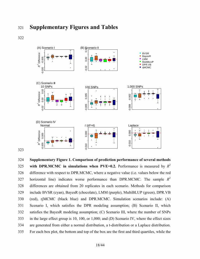
Supplementary Figure 1. Comparison of prediction performance of several methods 324
with DPR.MCMC in simulations when PVE=0.2. Performance is measured by R2 325
difference with respect to DPR.MCMC, where a negative value (i.e. values below the red 326
horizontal line) indicates worse performance than DPR.MCMC. The sample R2 327
differences are obtained from 20 replicates in each scenario. Methods for comparison 328
include BVSR (cyan), BayesR (chocolate), LMM (purple), MultiBLUP (green), DPR.VB 329
(red), rjMCMC (black blue) and DPR.MCMC. Simulation scenarios include: (A) 330
Scenario I, which satisfies the DPR modeling assumption; (B) Scenario II, which 331
satisfies the BayesR modeling assumption; (C) Scenario III, where the number of SNPs 332
in the large effect group is 10, 100, or 1,000; and (D) Scenario IV, where the effect sizes 333
are generated from either a normal distribution, a t-distribution or a Laplace distribution. 334
For each box plot, the bottom and top of the box are the first and third quartiles, while the 335

19/44
ends of whiskers represent either the lowest datum within 1.5 interquartile range of the 336
lower quartile or the highest datum within 1.5 interquartile range of the upper quartile. 337
For DPR.MCMC, the mean predictive R2 in the test set and the standard deviation for the 338
eight settings are respectively 0.074 (0.020), 0.081 (0.016), 0.076 (0.018), 0.072 (0.019), 339
0.064 (0.016), 0.083 (0.023), 0.077 (0.016) and 0.077 (0.017). 340
341
342
343
344
345
346
347
348
349
350
351
352
353
354
355
20/44
-0.0
6-0
.02
R2 D
iffer
ence
(A) Scenario I
-0.1
2-0
.06
0.00
(B) Scenario IIBVSRBayesRLMMMultiBLUPDPR.VBrjMCMC
-0.0
8-0
.04
0.00
R2 D
iffer
ence
(C) Scenario III 10 SNPs
-0.0
3-0
.01
100 SNPs
-0.0
150.
000
1,000 SNPs
-0.0
3-0
.01
R2 D
iffer
ence
(D) Scenario IV Normal
-0.0
20-0
.005
t (df=4)
-0.0
20-0
.005
Laplace
356
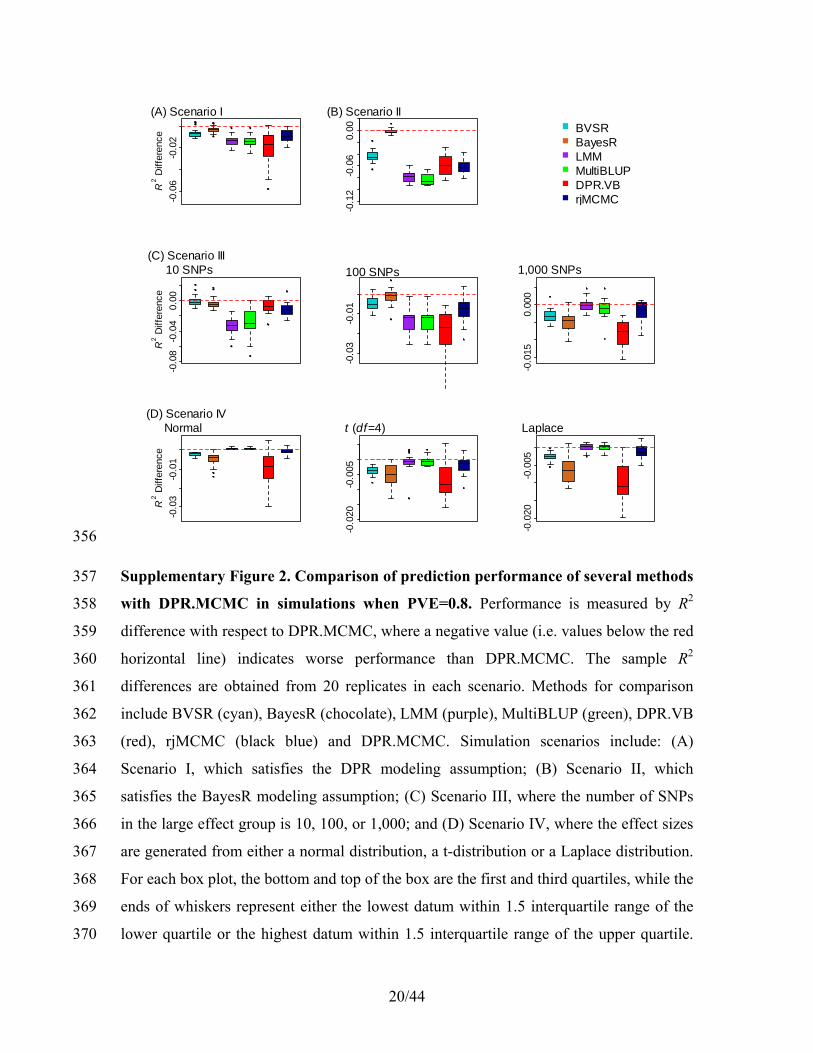
Supplementary Figure 2. Comparison of prediction performance of several methods 357
with DPR.MCMC in simulations when PVE=0.8. Performance is measured by R2 358
difference with respect to DPR.MCMC, where a negative value (i.e. values below the red 359
horizontal line) indicates worse performance than DPR.MCMC. The sample R2 360
differences are obtained from 20 replicates in each scenario. Methods for comparison 361
include BVSR (cyan), BayesR (chocolate), LMM (purple), MultiBLUP (green), DPR.VB 362
(red), rjMCMC (black blue) and DPR.MCMC. Simulation scenarios include: (A) 363
Scenario I, which satisfies the DPR modeling assumption; (B) Scenario II, which 364
satisfies the BayesR modeling assumption; (C) Scenario III, where the number of SNPs 365
in the large effect group is 10, 100, or 1,000; and (D) Scenario IV, where the effect sizes 366
are generated from either a normal distribution, a t-distribution or a Laplace distribution. 367
For each box plot, the bottom and top of the box are the first and third quartiles, while the 368
ends of whiskers represent either the lowest datum within 1.5 interquartile range of the 369
lower quartile or the highest datum within 1.5 interquartile range of the upper quartile. 370

21/44
For DPR.MCMC, the mean predictive R2 in the test set and the standard deviation for the 371
eight settings are respectively 0.554 (0.028), 0.622 (0.022), 0.569 (0.023), 0.548 (0.027), 372
0.537 (0.030), 0.543 (0.028), 0.546 (0.027) and 0.539 (0.022). 373
374
375
376
377
378
379
380
381
382
22/44
-0.0
100.
005
0.02
0M
SE
Diff
eren
ce
(A) Scenario I
-0.0
150.
000
0.01
5
(B) Scenario II
BVSRBayesRLMMMultiBLUPDPR.VBrjMCMC
-0.0
20.
00M
SE
Diff
eren
ce
(C) Scenario III 10 SNPs
-0.0
150.
000
100 SNPs
-0.0
050.
010
1,000 SNPs
-0.0
050.
005
MS
E D
iffer
ence
(D) Scenario IV Normal
-0.0
050.
005
t (df=4)
-0.0
050.
010
Laplace
383
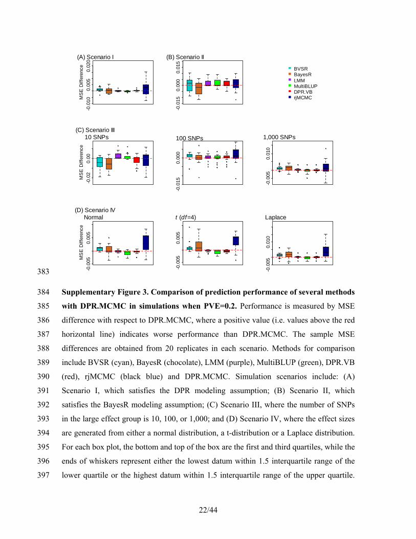
Supplementary Figure 3. Comparison of prediction performance of several methods 384
with DPR.MCMC in simulations when PVE=0.2. Performance is measured by MSE 385
difference with respect to DPR.MCMC, where a positive value (i.e. values above the red 386
horizontal line) indicates worse performance than DPR.MCMC. The sample MSE 387
differences are obtained from 20 replicates in each scenario. Methods for comparison 388
include BVSR (cyan), BayesR (chocolate), LMM (purple), MultiBLUP (green), DPR.VB 389
(red), rjMCMC (black blue) and DPR.MCMC. Simulation scenarios include: (A) 390
Scenario I, which satisfies the DPR modeling assumption; (B) Scenario II, which 391
satisfies the BayesR modeling assumption; (C) Scenario III, where the number of SNPs 392
in the large effect group is 10, 100, or 1,000; and (D) Scenario IV, where the effect sizes 393
are generated from either a normal distribution, a t-distribution or a Laplace distribution. 394
For each box plot, the bottom and top of the box are the first and third quartiles, while the 395
ends of whiskers represent either the lowest datum within 1.5 interquartile range of the 396
lower quartile or the highest datum within 1.5 interquartile range of the upper quartile. 397

23/44
For DPR.MCMC, the mean predictive MSE in the test set and the standard deviation for 398
the eight settings are respectively 0.919 (0.044), 0.910 (0.038), 0.929 (0.036), 0.944 399
(0.053), 0.923 (0.038), 0.925 (0.033), 0.924 (0.037) and 0.918 (0.037). 400
401
402
403
404
405
406
407
408
409
24/44
-0.0
20-0
.005
0.01
0M
SE
Diff
eren
ce
(A) Scenario I
-0.0
40.
000.
04
(B) Scenario II
BVSRBayesRLMMMultiBLUPDPR.VBrjMCMC
0.00
0.04
MS
E D
iffer
ence
(C) Scenario III 10 SNPs
-0.0
10.
010.
03
100 SNPs
-0.0
100.
005
1,000 SNPs
-0.0
100.
005
MS
E D
iffer
ence
(D) Scenario IV Normal
-0.0
050.
010
t (df=4)
-0.0
100.
005
Laplace
410
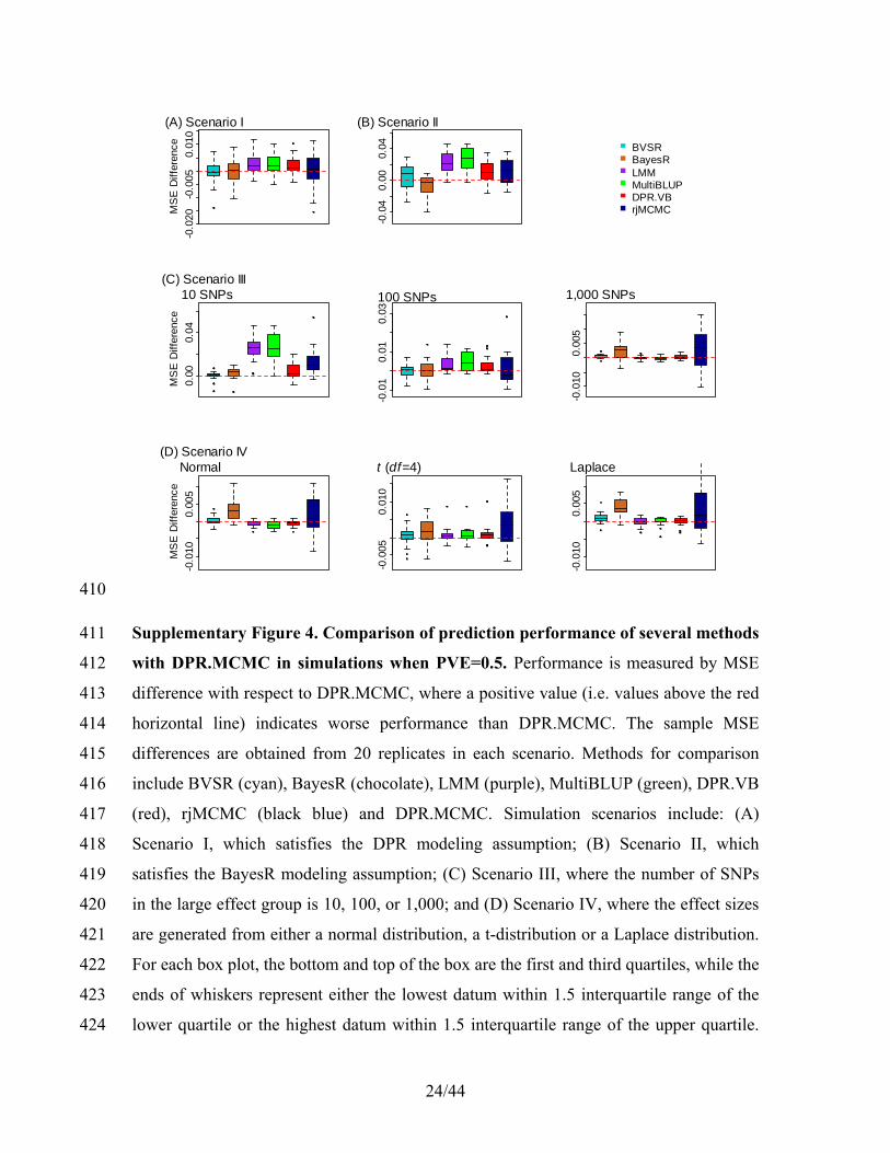
Supplementary Figure 4. Comparison of prediction performance of several methods 411
with DPR.MCMC in simulations when PVE=0.5. Performance is measured by MSE 412
difference with respect to DPR.MCMC, where a positive value (i.e. values above the red 413
horizontal line) indicates worse performance than DPR.MCMC. The sample MSE 414
differences are obtained from 20 replicates in each scenario. Methods for comparison 415
include BVSR (cyan), BayesR (chocolate), LMM (purple), MultiBLUP (green), DPR.VB 416
(red), rjMCMC (black blue) and DPR.MCMC. Simulation scenarios include: (A) 417
Scenario I, which satisfies the DPR modeling assumption; (B) Scenario II, which 418
satisfies the BayesR modeling assumption; (C) Scenario III, where the number of SNPs 419
in the large effect group is 10, 100, or 1,000; and (D) Scenario IV, where the effect sizes 420
are generated from either a normal distribution, a t-distribution or a Laplace distribution. 421
For each box plot, the bottom and top of the box are the first and third quartiles, while the 422
ends of whiskers represent either the lowest datum within 1.5 interquartile range of the 423
lower quartile or the highest datum within 1.5 interquartile range of the upper quartile. 424

25/44
For DPR.MCMC, the mean predictive MSE in the test set and the standard deviation for 425
the eight settings are respectively 0.722 (0.043), 0.701 (0.028), 0.707 (0.034), 0.717 426
(0.037), 0.727 (0.034), 0.734 (0.040), 0.721 (0.032) and 0.720 (0.028). 427
428
429
430
431
432
433
434
435
436
437
26/44
0.00
0.04
MS
E D
iffer
ence
(A) Scenario I
0.00
0.06
(B) Scenario II
BVSRBayesRLMMMultiBLUPDPR.VBrjMCMC
-0.0
40.
000.
04M
SE
Diff
eren
ce
(C) Scenario III 10 SNPs
0.00
0.04
100 SNPs
-0.0
050.
010
0.02
5 1,000 SNPs
-0.0
10.
010.
03M
SE
Diff
eren
ce
(D) Scenario IV Normal
-0.0
10.
010.
03
t (df=4)
-0.0
100.
005
0.02
0 Laplace
438
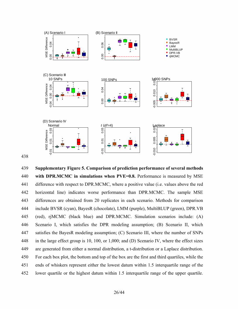
Supplementary Figure 5. Comparison of prediction performance of several methods 439
with DPR.MCMC in simulations when PVE=0.8. Performance is measured by MSE 440
difference with respect to DPR.MCMC, where a positive value (i.e. values above the red 441
horizontal line) indicates worse performance than DPR.MCMC. The sample MSE 442
differences are obtained from 20 replicates in each scenario. Methods for comparison 443
include BVSR (cyan), BayesR (chocolate), LMM (purple), MultiBLUP (green), DPR.VB 444
(red), rjMCMC (black blue) and DPR.MCMC. Simulation scenarios include: (A) 445
Scenario I, which satisfies the DPR modeling assumption; (B) Scenario II, which 446
satisfies the BayesR modeling assumption; (C) Scenario III, where the number of SNPs 447
in the large effect group is 10, 100, or 1,000; and (D) Scenario IV, where the effect sizes 448
are generated from either a normal distribution, a t-distribution or a Laplace distribution. 449
For each box plot, the bottom and top of the box are the first and third quartiles, while the 450
ends of whiskers represent either the lowest datum within 1.5 interquartile range of the 451
lower quartile or the highest datum within 1.5 interquartile range of the upper quartile. 452

27/44
For DPR.MCMC, the mean predictive MSE in the test set and the standard deviation for 453
the eight settings are respectively 0.443 (0.032), 0.379 (0.016), 0.429 (0.024), 0.454 454
(0.023), 0.464 (0.030), 0.465 (0.027), 0.454 (0.032) and 0.457 (0.022). 455
456
457
458
459
460
461
462
463
464
465
466
467
468
469
470
471
28/44
472
473
474
475
29/44
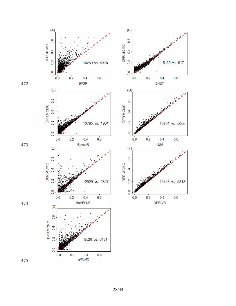
Supplementary Figure 6. Comparison of predictive R2 from DPR.MCMC with the 476
other six methods for predicting gene expression levels in the GEUVADIS data. 477
Scatter plots show (A) predictive R2 in the test data obtained by DPR.MCMC vs that 478
obtained by BVSR for all genes; (B) DPR.MCMC vs ENET; (C) DPR.MCMC vs 479
BayesR; (D) DPR.MCMC vs LMM; (E) DPR.MCMC vs MultiBLUP; (F) DPR.MCMC 480
vs DPR.VB; (G) DPR.MCMC vs rjMCMC. Each panel also lists the number of genes 481
where DPR.MCMC performs better (first number) and the number of genes where 482
DPR.MCMC performs worse (second number). 483
484
485
486
487
488
489
490
491
492
493
494
495
496
497
498
499
500
501
502
503
504
505
30/44
506
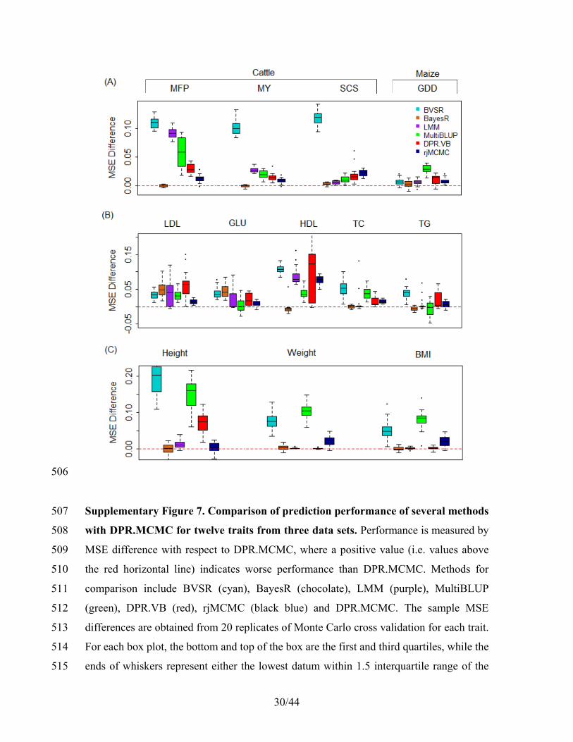
Supplementary Figure 7. Comparison of prediction performance of several methods 507
with DPR.MCMC for twelve traits from three data sets. Performance is measured by 508
MSE difference with respect to DPR.MCMC, where a positive value (i.e. values above 509
the red horizontal line) indicates worse performance than DPR.MCMC. Methods for 510
comparison include BVSR (cyan), BayesR (chocolate), LMM (purple), MultiBLUP 511
(green), DPR.VB (red), rjMCMC (black blue) and DPR.MCMC. The sample MSE 512
differences are obtained from 20 replicates of Monte Carlo cross validation for each trait. 513
For each box plot, the bottom and top of the box are the first and third quartiles, while the 514
ends of whiskers represent either the lowest datum within 1.5 interquartile range of the 515
31/44
lower quartile or the highest datum within 1.5 interquartile range of the upper quartile. 516
For DPR.MCMC, the mean predictive MSE in the test set and the standard deviation are 517
0.246 (0.011) for MFP, 0.371 (0.019) for MY, 0.446 (0.028) for SCS, 0.170 (0.012) for 518
GDD, 0.928 (0.029) for LDL, 0.954 (0.034) for GLU, 0.833 (0.063) for HDL, 0.970 519
(0.044) for TC, 0.960 (0.035) for TG, 0.519 (0.050) for height, 0.834 (0.065) for weight 520
and 0.868 (0.074) for BMI. The SNP heritability estimates are 0.912 (0.007) for MFP, 521
0.810 (0.012) for MY, 0.801 (0.012) for SCS, 0.880 (0.013) for GDD, 0.397 (0.024) for 522
LDL, 0.357 (0.036) for GLU, 0.418 (0.024) for HDL, 0.402 (0.036) for TC, 0.334 (0.034) 523
for TG, 0.905 (0.013) for Height, 0.548 (0.022) for Weight and 0.483 (0.023) for BMI. 524
525
526
527
528
529
530
531
532
533
534
535
536
537
538
539
540
541
542
543
544
545
546
32/44
547
548
33/44
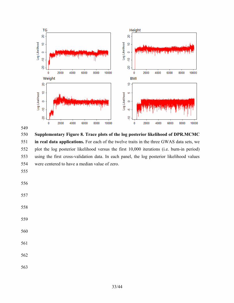
549
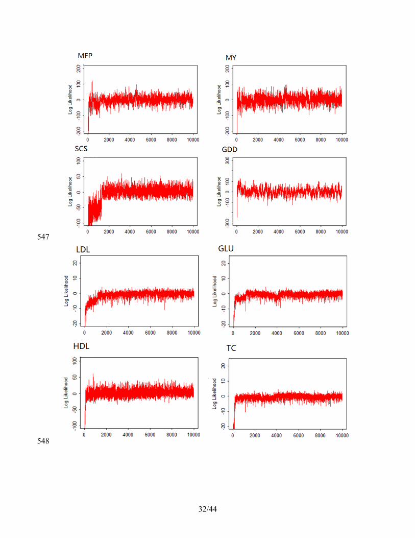
Supplementary Figure 8. Trace plots of the log posterior likelihood of DPR.MCMC 550
in real data applications. For each of the twelve traits in the three GWAS data sets, we 551
plot the log posterior likelihood versus the first 10,000 iterations (i.e. burn-in period) 552
using the first cross-validation data. In each panel, the log posterior likelihood values 553
were centered to have a median value of zero. 554
555
556
557
558
559
560
561
562
563
34/44
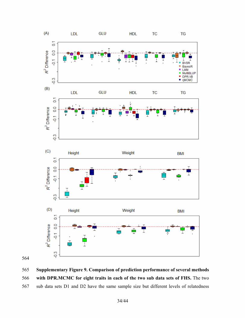
564
Supplementary Figure 9. Comparison of prediction performance of several methods 565
with DPR.MCMC for eight traits in each of the two sub data sets of FHS. The two 566
sub data sets D1 and D2 have the same sample size but different levels of relatedness 567
35/44
(individuals in D1 are more related to each other than those in D2). (A) The R2 difference 568
of five plasma traits (LDL, GLU, HDL, TC and TG) with respect to DPR.MCMC in the 569
D1 and D2 sub data of FHS; (B) The R2 difference of three anthropometric traits (Height, 570
Weight and BMI) with respect to DPR.MCMC in the D1 and D2 sub data of FHS. For 571
each box plot, the bottom and top of the box are the first and third quartiles, while the 572
ends of whiskers represent either the lowest datum within 1.5 interquartile range of the 573
lower quartile or the highest datum within 1.5 interquartile range of the upper quartile. 574
FHS: Framingham heart study. 575
576
36/44
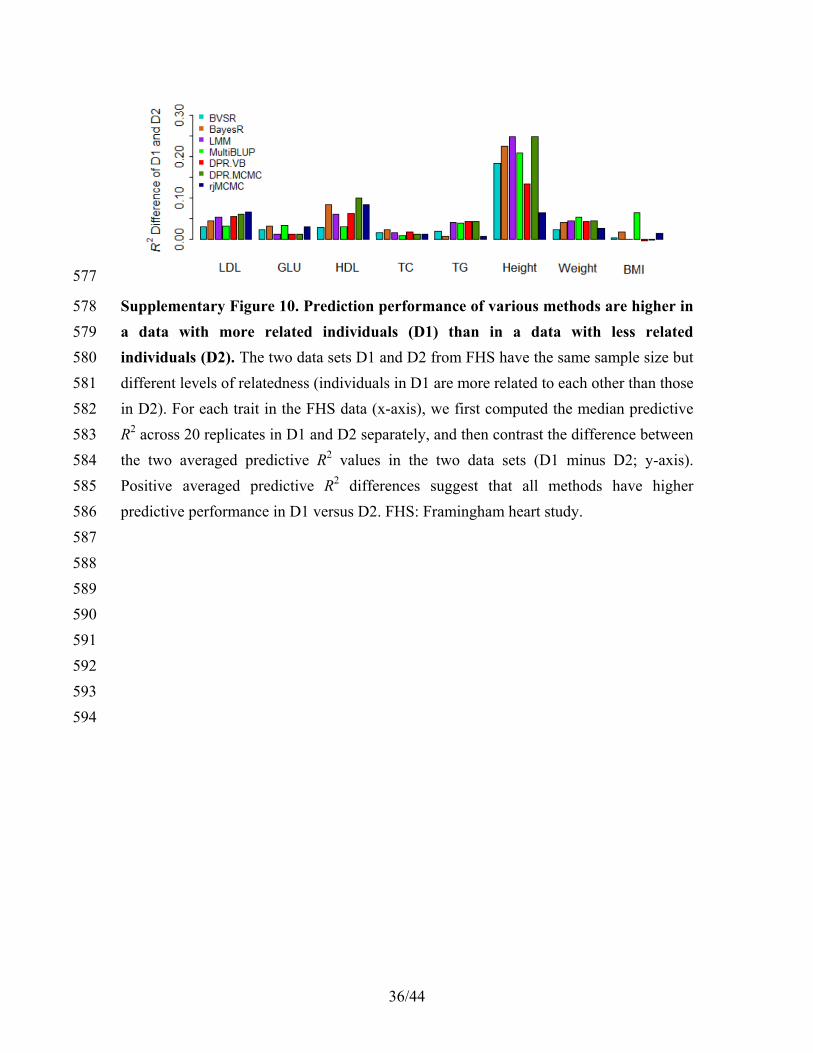
577
Supplementary Figure 10. Prediction performance of various methods are higher in 578
a data with more related individuals (D1) than in a data with less related 579
individuals (D2). The two data sets D1 and D2 from FHS have the same sample size but 580
different levels of relatedness (individuals in D1 are more related to each other than those 581
in D2). For each trait in the FHS data (x-axis), we first computed the median predictive 582
R2 across 20 replicates in D1 and D2 separately, and then contrast the difference between 583
the two averaged predictive R2 values in the two data sets (D1 minus D2; y-axis). 584
Positive averaged predictive R2 differences suggest that all methods have higher 585
predictive performance in D1 versus D2. FHS: Framingham heart study. 586
587
588
589
590
591
592
593
594
37/44
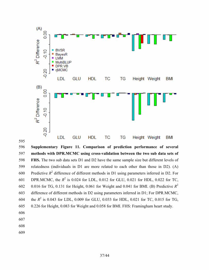
595
Supplementary Figure 11. Comparison of prediction performance of several 596
methods with DPR.MCMC using cross-validation between the two sub data sets of 597
FHS. The two sub data sets D1 and D2 have the same sample size but different levels of 598
relatedness (individuals in D1 are more related to each other than those in D2). (A) 599
Predictive R2 difference of different methods in D1 using parameters inferred in D2. For 600
DPR.MCMC, the R2 is 0.024 for LDL, 0.012 for GLU, 0.021 for HDL, 0.022 for TC, 601
0.016 for TG, 0.131 for Height, 0.061 for Weight and 0.041 for BMI. (B) Predictive R2 602
difference of different methods in D2 using parameters inferred in D1; For DPR.MCMC, 603
the R2 is 0.043 for LDL, 0.009 for GLU, 0.033 for HDL, 0.021 for TC, 0.015 for TG, 604
0.226 for Height, 0.083 for Weight and 0.058 for BMI. FHS: Framingham heart study. 605
606
607
608
609
38/44
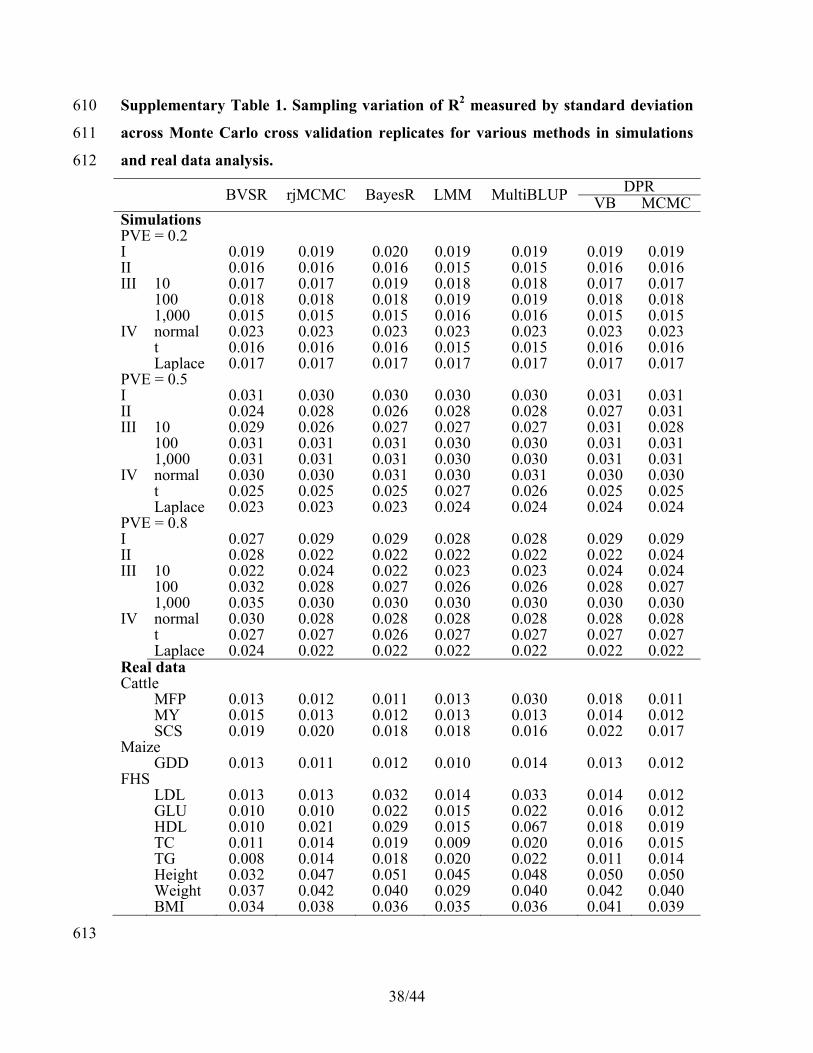
Supplementary Table 1. Sampling variation of R2 measured by standard deviation 610
across Monte Carlo cross validation replicates for various methods in simulations 611
and real data analysis. 612
BVSR rjMCMC BayesR LMM MultiBLUP DPRVB MCMC
Simulations PVE = 0.2
I 0.019 0.019 0.020 0.019 0.019 0.019 0.019II 0.016 0.016 0.016 0.015 0.015 0.016 0.016III 10 0.017 0.017 0.019 0.018 0.018 0.017 0.017 100 0.018 0.018 0.018 0.019 0.019 0.018 0.018 1,000 0.015 0.015 0.015 0.016 0.016 0.015 0.015IV normal 0.023 0.023 0.023 0.023 0.023 0.023 0.023 t 0.016 0.016 0.016 0.015 0.015 0.016 0.016 Laplace 0.017 0.017 0.017 0.017 0.017 0.017 0.017PVE = 0.5 I 0.031 0.030 0.030 0.030 0.030 0.031 0.031II 0.024 0.028 0.026 0.028 0.028 0.027 0.031III 10 0.029 0.026 0.027 0.027 0.027 0.031 0.028 100 0.031 0.031 0.031 0.030 0.030 0.031 0.031 1,000 0.031 0.031 0.031 0.030 0.030 0.031 0.031IV normal 0.030 0.030 0.031 0.030 0.031 0.030 0.030 t 0.025 0.025 0.025 0.027 0.026 0.025 0.025 Laplace 0.023 0.023 0.023 0.024 0.024 0.024 0.024PVE = 0.8 I 0.027 0.029 0.029 0.028 0.028 0.029 0.029II 0.028 0.022 0.022 0.022 0.022 0.022 0.024III 10 0.022 0.024 0.022 0.023 0.023 0.024 0.024 100 0.032 0.028 0.027 0.026 0.026 0.028 0.027 1,000 0.035 0.030 0.030 0.030 0.030 0.030 0.030IV normal 0.030 0.028 0.028 0.028 0.028 0.028 0.028 t 0.027 0.027 0.026 0.027 0.027 0.027 0.027 Laplace 0.024 0.022 0.022 0.022 0.022 0.022 0.022Real data Cattle
MFP 0.013 0.012 0.011 0.013 0.030 0.018 0.011 MY 0.015 0.013 0.012 0.013 0.013 0.014 0.012 SCS 0.019 0.020 0.018 0.018 0.016 0.022 0.017Maize GDD 0.013 0.011 0.012 0.010 0.014 0.013 0.012FHS LDL 0.013 0.013 0.032 0.014 0.033 0.014 0.012 GLU 0.010 0.010 0.022 0.015 0.022 0.016 0.012 HDL 0.010 0.021 0.029 0.015 0.067 0.018 0.019 TC 0.011 0.014 0.019 0.009 0.020 0.016 0.015 TG 0.008 0.014 0.018 0.020 0.022 0.011 0.014 Height 0.032 0.047 0.051 0.045 0.048 0.050 0.050 Weight 0.037 0.042 0.040 0.029 0.040 0.042 0.040 BMI 0.034 0.038 0.036 0.035 0.036 0.041 0.039
613
39/44
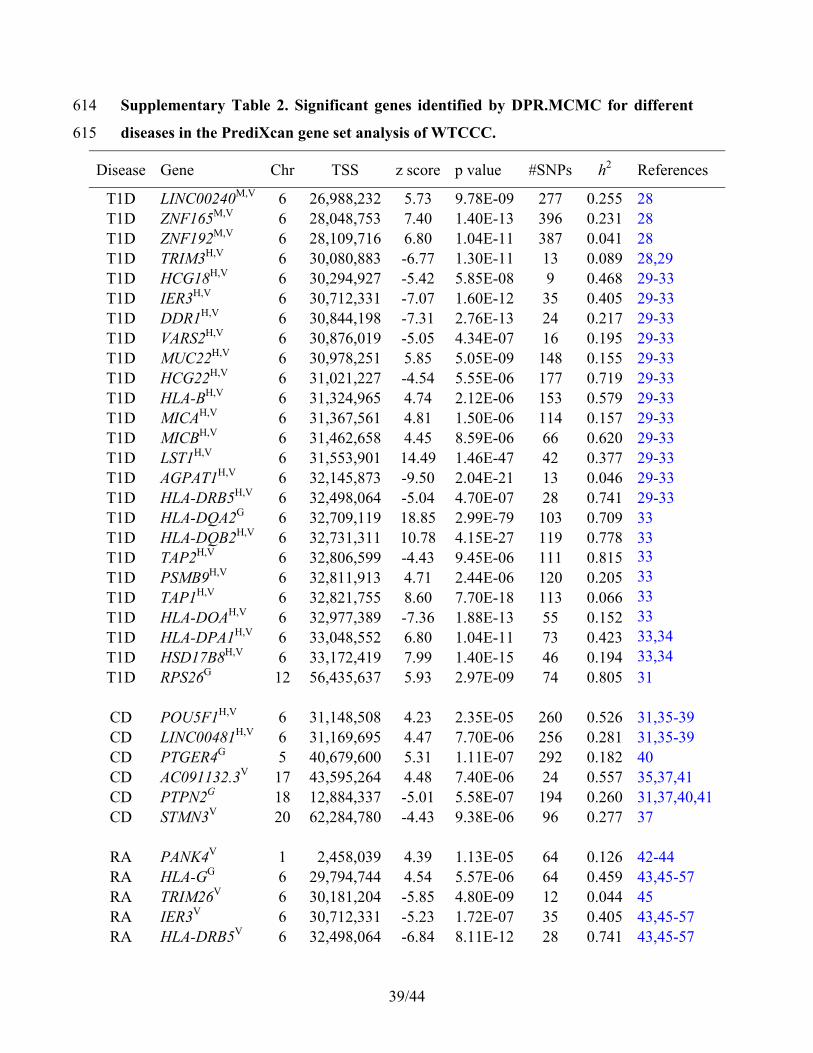
Supplementary Table 2. Significant genes identified by DPR.MCMC for different 614
diseases in the PrediXcan gene set analysis of WTCCC. 615
Disease Gene Chr TSS z score p value #SNPs h2 References
T1D LINC00240M,V 6 26,988,232 5.73 9.78E-09 277 0.255 28 T1D ZNF165M,V 6 28,048,753 7.40 1.40E-13 396 0.231 28 T1D ZNF192M,V 6 28,109,716 6.80 1.04E-11 387 0.041 28 T1D TRIM3H,V 6 30,080,883 -6.77 1.30E-11 13 0.089 28,29 T1D HCG18H,V 6 30,294,927 -5.42 5.85E-08 9 0.468 29-33 T1D IER3H,V 6 30,712,331 -7.07 1.60E-12 35 0.405 29-33 T1D DDR1H,V 6 30,844,198 -7.31 2.76E-13 24 0.217 29-33 T1D VARS2H,V 6 30,876,019 -5.05 4.34E-07 16 0.195 29-33 T1D MUC22H,V 6 30,978,251 5.85 5.05E-09 148 0.155 29-33 T1D HCG22H,V 6 31,021,227 -4.54 5.55E-06 177 0.719 29-33 T1D HLA-BH,V 6 31,324,965 4.74 2.12E-06 153 0.579 29-33 T1D MICAH,V 6 31,367,561 4.81 1.50E-06 114 0.157 29-33 T1D MICBH,V 6 31,462,658 4.45 8.59E-06 66 0.620 29-33 T1D LST1H,V 6 31,553,901 14.49 1.46E-47 42 0.377 29-33 T1D AGPAT1H,V 6 32,145,873 -9.50 2.04E-21 13 0.046 29-33 T1D HLA-DRB5H,V 6 32,498,064 -5.04 4.70E-07 28 0.741 29-33 T1D HLA-DQA2G 6 32,709,119 18.85 2.99E-79 103 0.709 33 T1D HLA-DQB2H,V 6 32,731,311 10.78 4.15E-27 119 0.778 33 T1D TAP2H,V 6 32,806,599 -4.43 9.45E-06 111 0.815 33 T1D PSMB9H,V 6 32,811,913 4.71 2.44E-06 120 0.205 33 T1D TAP1H,V 6 32,821,755 8.60 7.70E-18 113 0.066 33 T1D HLA-DOAH,V 6 32,977,389 -7.36 1.88E-13 55 0.152 33 T1D HLA-DPA1H,V 6 33,048,552 6.80 1.04E-11 73 0.423 33,34 T1D HSD17B8H,V 6 33,172,419 7.99 1.40E-15 46 0.194 33,34 T1D RPS26G 12 56,435,637 5.93 2.97E-09 74 0.805 31
CD POU5F1H,V 6 31,148,508 4.23 2.35E-05 260 0.526 31,35-39 CD LINC00481H,V 6 31,169,695 4.47 7.70E-06 256 0.281 31,35-39 CD PTGER4G 5 40,679,600 5.31 1.11E-07 292 0.182 40 CD AC091132.3V 17 43,595,264 4.48 7.40E-06 24 0.557 35,37,41 CD PTPN2G 18 12,884,337 -5.01 5.58E-07 194 0.260 31,37,40,41 CD STMN3V 20 62,284,780 -4.43 9.38E-06 96 0.277 37
RA PANK4V 1 2,458,039 4.39 1.13E-05 64 0.126 42-44 RA HLA-GG 6 29,794,744 4.54 5.57E-06 64 0.459 43,45-57 RA TRIM26V 6 30,181,204 -5.85 4.80E-09 12 0.044 45 RA IER3V 6 30,712,331 -5.23 1.72E-07 35 0.405 43,45-57 RA HLA-DRB5V 6 32,498,064 -6.84 8.11E-12 28 0.741 43,45-57
40/44
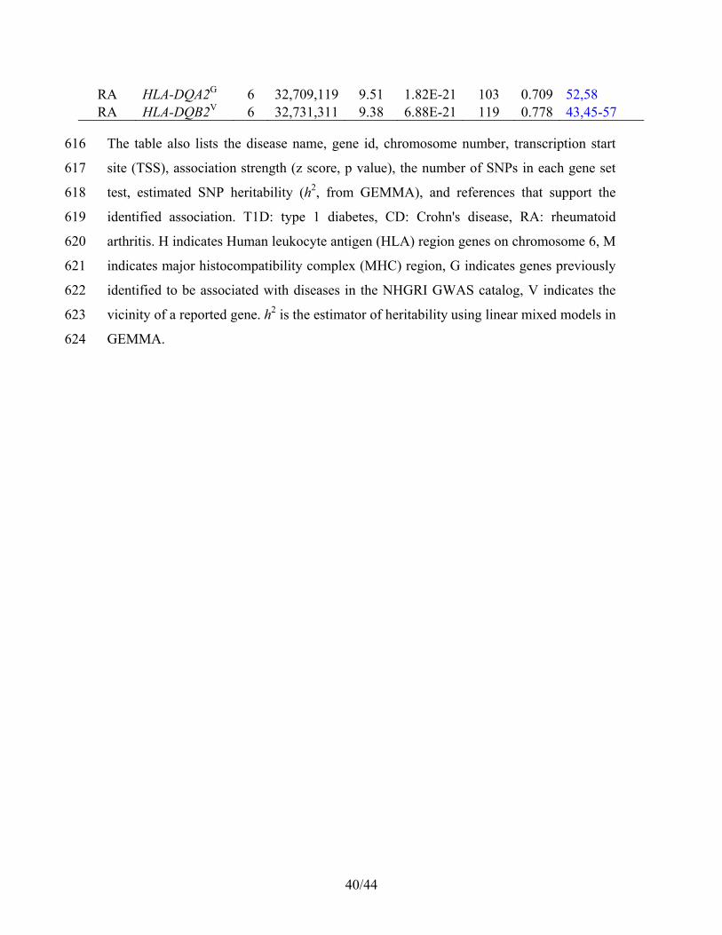
RA HLA-DQA2G 6 32,709,119 9.51 1.82E-21 103 0.709 52,58 RA HLA-DQB2V 6 32,731,311 9.38 6.88E-21 119 0.778 43,45-57
The table also lists the disease name, gene id, chromosome number, transcription start 616
site (TSS), association strength (z score, p value), the number of SNPs in each gene set 617
test, estimated SNP heritability (h2, from GEMMA), and references that support the 618
identified association. T1D: type 1 diabetes, CD: Crohn's disease, RA: rheumatoid 619
arthritis. H indicates Human leukocyte antigen (HLA) region genes on chromosome 6, M 620
indicates major histocompatibility complex (MHC) region, G indicates genes previously 621
identified to be associated with diseases in the NHGRI GWAS catalog, V indicates the 622
vicinity of a reported gene. h2 is the estimator of heritability using linear mixed models in 623
GEMMA.624
41/44
Supplementary References 625
1. Zhou, X., Carbonetto, P., & Stephens, M. Polygenic modeling with Bayesian 626 sparse linear mixed models. PLoS Genet. 9, e1003264 (2013). 627
2. Yang, J. et al. Common SNPs explain a large proportion of the heritability for 628 human height. Nat. Genet. 42, 565-569 (2010). 629
3. Moser, G. et al. Simultaneous Discovery, Estimation and Prediction Analysis of 630 Complex Traits Using a Bayesian Mixture Model. PLoS Genet. 11, e1004969 631 (2015). 632
4. Robert, C., & Casella, G. Monte Carlo statistical methods (Second ed.). New 633 York: Springer (2002). 634
5. Gelman, A. Parameterization and Bayesian Modeling. J. Am. Stat. Assoc. 99, 537-635 545 (2004). 636
6. Visscher, P. M., Hill, W. G., & Wray, N. R. Heritability in the genomics era--637 concepts and misconceptions. Nat. Rev. Genet. 9, 255-266 (2008). 638
7. de los Campos, G., Sorensen, D., & Gianola, D. Genomic heritability: what is it? 639 PLoS Genet. 11, e1005048 (2015). 640
8. Zhou, X., & Stephens, M. Genome-wide efficient mixed-model analysis for 641 association studies. Nat. Genet. 44, 821-824 (2012). 642
9. Lippert, C. et al. FaST linear mixed models for genome-wide association studies. 643 Nat. Methods 8, 833-835 (2011). 644
10. Levine, R. A., & Casella, G. Optimizing random scan Gibbs samplers. J. 645 Multivariate Anal. 97, 2071-2100 (2006). 646
11. Levine, R. A., Yu, Z., Hanley, W. G., & Nitao, J. J. Implementing random scan 647 Gibbs samplers. Comput Stat 20, 177-196 (2005). 648
12. Blei, D. M., & Jordan, M. I. Variational inference for Dirichlet process mixtures. 649 Bayesian. Anal. 1, 121-143 (2006). 650
13. Ishwaran, H., & James, L. F. Approximate Dirichlet Process Computing in Finite 651 Normal Mixtures. J. Comput. Graph. Statist. 11, 508-532 (2002). 652
14. Ishwaran, H., & James, L. F. Gibbs sampling methods for stick-breaking priors. J. 653 Am. Stat. Assoc. 96, (2001). 654
15. Gelman, A. et al. Bayesian Data Analysis (Third ed.). New York: Chapman & 655 Hall/CRC (2013). 656
16. Spiegelhalter, D. J., Best, N. G., Carlin, B. P., & Van Der Linde, A. Bayesian 657 measures of model complexity and fit. J. R. Stat. Soc. Ser. B. 64, 583-639 (2002). 658
17. Gelman, A., Hwang, J., & Vehtari, A. Understanding predictive information 659 criteria for Bayesian models. Stat. Comput. 24, 997-1016 (2014). 660
18. Brooks, S. Markov chain Monte Carlo method and its application. Journal of the 661 royal statistical society: series D (the Statistician) 47, 69-100 (1998). 662
19. Hastie, T., Tibshirani, R., & Friedman, J. H. The elements of statistical learning: 663 data mining, inference, and prediction. New York, NY: Springer (2009). 664
20. Bishop, C. M. Pattern recognition and machine learning. New York: Springer 665 (2006). 666
21. Jordan, M. I., Ghahramani, Z., Jaakkola, T. S., & Saul, L. K. An introduction to 667 variational methods for graphical models. Mach. Learn. 37, 183-233 (1999). 668
22. Grimmer, J. An Introduction to Bayesian Inference via Variational 669 Approximations. Pol. Anal. 19, 32-47 (2011). 670

42/44
23. Ormerod, J. T., & Wand, M. Explaining variational approximations. Am. Stat. 64, 671 140-153 (2010). 672
24. Pham, T. H., Ormerod, J. T., & Wand, M. P. Mean field variational Bayesian 673 inference for nonparametric regression with measurement error. Comput. Stat. 674 Data Anal. 68, 375-387 (2013). 675
25. Wand, M. P., Ormerod, J. T., Padoan, S. A., & Fuhrwirth, R. Mean field 676 variational Bayes for elaborate distributions. Bayesian. Anal. 6, 847-900 (2011). 677
26. Blei, D. M., Kucukelbir, A., & McAuliffe, J. D. Variational inference: A review 678 for statisticians. J. Am. Stat. Assoc. (in press), Preprint at 679 https://arxiv.org/abs/1601.00670 (2017). 680
27. Wang, C., & Blei, D. M. Variational inference in nonconjugate models. J. Mach. 681 Learn. Res. 14, 1005-1031 (2013). 682
28. DIAbetes Genetics Replication And Meta-analysis (DIAGRAM) Consortium et 683 al. Genome-wide trans-ancestry meta-analysis provides insight into the genetic 684 architecture of type 2 diabetes susceptibility. Nat. Genet. 46, 234-244 (2014). 685
29. Barrett, J. C. et al. Genome-wide association study and meta-analysis find that 686 over 40 loci affect risk of type 1 diabetes. Nat. Genet. 41, 703-707 (2009). 687
30. Cooper, J. D. et al. Meta-analysis of genome-wide association study data 688 identifies additional type 1 diabetes risk loci. Nat. Genet. 40, 1399-1401 (2008). 689
31. The Wellcome Trust Case Control Consortium. Genome-wide association study 690 of 14,000 cases of seven common diseases and 3,000 shared controls. Nature 447, 691 661-678 (2007). 692
32. Hakonarson, H. et al. A genome-wide association study identifies KIAA0350 as a 693 type 1 diabetes gene. Nature 448, 591-594 (2007). 694
33. Perry, J. R. et al. Stratifying type 2 diabetes cases by BMI identifies genetic risk 695 variants in LAMA1 and enrichment for risk variants in lean compared to obese 696 cases. PLoS Genet. 8, e1002741 (2012). 697
34. Lin, H. et al. Novel susceptibility genes associated with diabetic cataract in a 698 Taiwanese population. Ophthalmic Genet. 34, 35-42 (2013). 699
35. Yamazaki, K. et al. A genome-wide association study identifies 2 susceptibility 700 loci for Crohn's disease in a Japanese population. Gastroenterology 144, 781-788 701 (2013). 702
36. Jostins, L. et al. Host-microbe interactions have shaped the genetic architecture of 703 inflammatory bowel disease. Nature 491, 119-124 (2012). 704
37. Franke, A. et al. Genome-wide meta-analysis increases to 71 the number of 705 confirmed Crohn's disease susceptibility loci. Nat. Genet. 42, 1118-1125 (2010). 706
38. Julià, A. et al. A genome-wide association study on a southern European 707 population identifies a new Crohn's disease susceptibility locus at RBX1-EP300. 708 Gut 62, 1440-1445 (2013). 709
39. Yang, S. K. et al. Genome-wide association study of Crohn's disease in Koreans 710 revealed three new susceptibility loci and common attributes of genetic 711 susceptibility across ethnic populations. Gut 63, 80-87 (2014). 712
40. Parkes, M. et al. Sequence variants in the autophagy gene IRGM and multiple 713 other replicating loci contribute to Crohn's disease susceptibility. Nat. Genet. 39, 714 830-832 (2007). 715
43/44
41. Barrett, J. C. et al. Genome-wide association defines more than 30 distinct 716 susceptibility loci for Crohn's disease. Nat. Genet. 40, 955-962 (2008). 717
42. Orozco, G. et al. Novel Rheumatoid Arthritis Susceptibility Locus at 22q12 718 Identified in an Extended UK Genome-Wide Association Study. Arthritis 719 Rheumatol. 66, 24-30 (2014). 720
43. Stahl, E. A. et al. Genome-wide association study meta-analysis identifies seven 721 new rheumatoid arthritis risk loci. Nat. Genet. 42, 508-514 (2010). 722
44. Raychaudhuri, S. et al. Common variants at CD40 and other loci confer risk of 723 rheumatoid arthritis. Nat. Genet. 40, 1216-1223 (2008). 724
45. Eleftherohorinou, H., Hoggart, C. J., Wright, V. J., Levin, M., & Coin, L. J. 725 Pathway-driven gene stability selection of two rheumatoid arthritis GWAS 726 identifies and validates new susceptibility genes in receptor mediated signalling 727 pathways. Hum. Mol. Genet. 20, 3494-3506 (2011). 728
46. Hüffmeier, U. et al. Common variants at TRAF3IP2 are associated with 729 susceptibility to psoriatic arthritis and psoriasis. Nat. Genet. 42, 996-999 (2010). 730
47. Bossini-Castillo, L. et al. A genome-wide association study of rheumatoid 731 arthritis without antibodies against citrullinated peptides. Ann. Rheum. Dis. 732 annrheumdis-2013-204591 (2014). 733
48. Hu, H.-J. et al. Common variants at the promoter region of the APOM confer a 734 risk of rheumatoid arthritis. Exp. Mol. Med. 43, 613-621 (2011). 735
49. Terao, C. et al. The human AIRE gene at chromosome 21q22 is a genetic 736 determinant for the predisposition to rheumatoid arthritis in Japanese population. 737 Hum. Mol. Genet. 20, 2680-2685 (2011). 738
50. Orozco, G. et al. Novel Rheumatoid Arthritis Susceptibility Locus at 22q12 739 Identified in an Extended UK Genome‐Wide Association Study. Arthritis 740 Rheumatol. 66, 24-30 (2014). 741
51. Behrens, E. M. et al. Association of the TRAF1–C5 locus on chromosome 9 with 742 juvenile idiopathic arthritis. Arthritis Rheum. 58, 2206-2207 (2008). 743
52. Nakajima, M. et al. New sequence variants in HLA class II/III region associated 744 with susceptibility to knee osteoarthritis identified by genome-wide association 745 study. PLoS ONE 5, e9723 (2010). 746
53. Okada, Y. et al. Genetics of rheumatoid arthritis contributes to biology and drug 747 discovery. Nature 506, 376-381 (2014). 748
54. Jiang, L. et al. Novel risk loci for rheumatoid arthritis in Han Chinese and 749 congruence with risk variants in Europeans. Arthritis Rheumatol. 66, 1121-1132 750 (2014). 751
55. Padyukov, L. et al. A genome-wide association study suggests contrasting 752 associations in ACPA-positive versus ACPA-negative rheumatoid arthritis. Ann. 753 Rheum. Dis. (2010). 754
56. Plenge, R. M. et al. TRAF1–C5 as a risk locus for rheumatoid arthritis—a 755 genomewide study. N. Engl. J. Med. 357, 1199-1209 (2007). 756
57. Freudenberg, J. et al. Genome-wide association study of rheumatoid arthritis in 757 Koreans: Population-specific loci as well as overlap with European susceptibility 758 loci. Arthritis Rheum. 63, 884-893 (2011). 759

44/44
58. Julia, A. et al. Genome‐wide association study of rheumatoid arthritis in the 760 Spanish population: KLF12 as a risk locus for rheumatoid arthritis susceptibility. 761 Arthritis Rheum. 58, 2275-2286 (2008). 762
763
764