fin 30220: macroeconomics the business cycle. billions of 2000 dollars $12,129b 2014q1 $1,938b...
TRANSCRIPT

FIN 30220: Macroeconomics
The Business Cycle
1947 1952 1957 1962 1967 1972 1977 1982 1987 1992 1997 2002 2007 20120
2000
4000
6000
8000
10000
12000
14000Bi
llion
s of
200
0 D
olla
rs
$12,129B2014Q1
$1,938B(1947Q1)
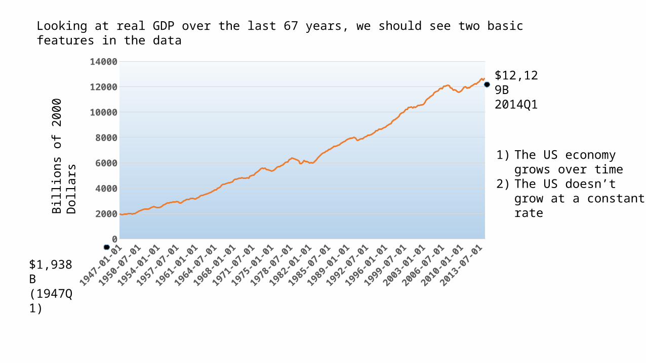
Looking at real GDP over the last 67 years, we should see two basic features in the data
1) The US economy grows over time
2) The US doesn’t grow at a constant rate
GDP
Time
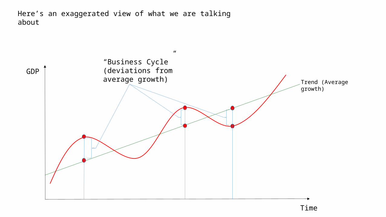
Trend (Average growth)
“Business Cycle” (deviations from average growth)
Here’s an exaggerated view of what we are talking about
GDP
Time
Trend (Average growth)
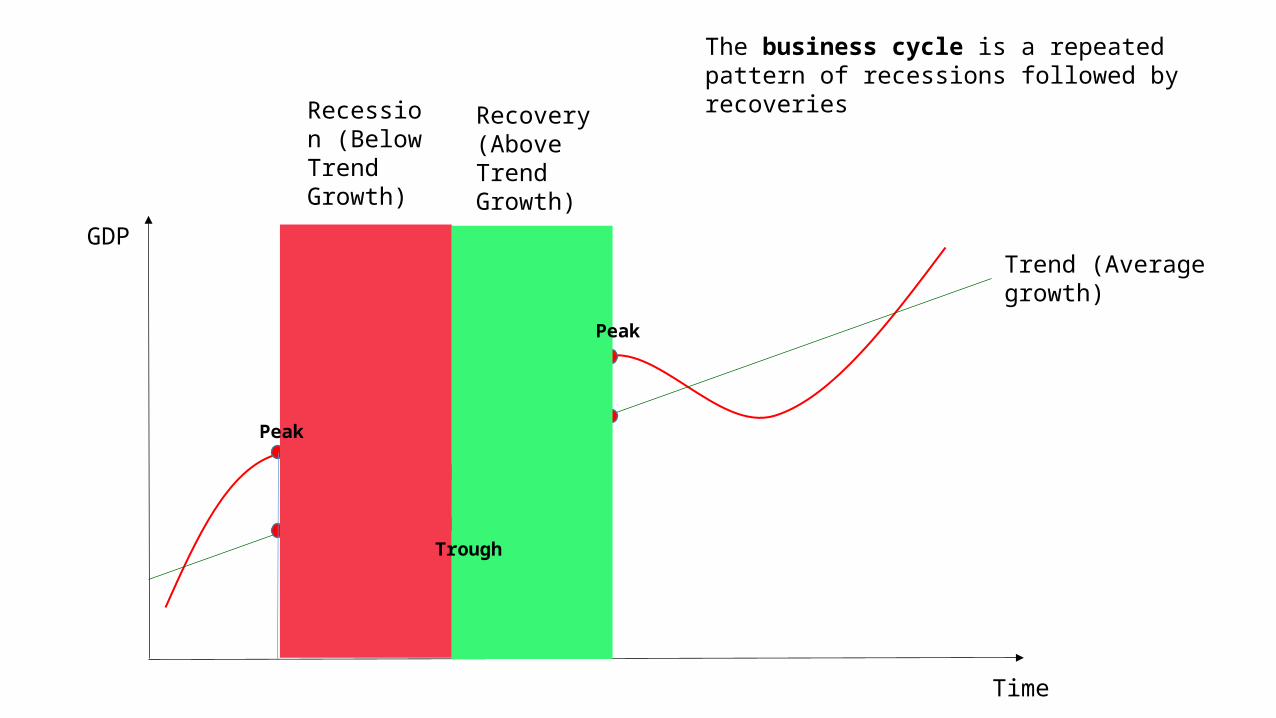
The business cycle is a repeated pattern of recessions followed by recoveries
Recession (Below Trend Growth)
Recovery (Above Trend Growth)
Peak
Trough
Peak

Once we have identified the trend, we can subtract it out to leave the cycle component all by itself.
GDP
Time
Trend (Average growth)
Actual GDP
Trend GDP
*100Actual Trend
DeviationTrend
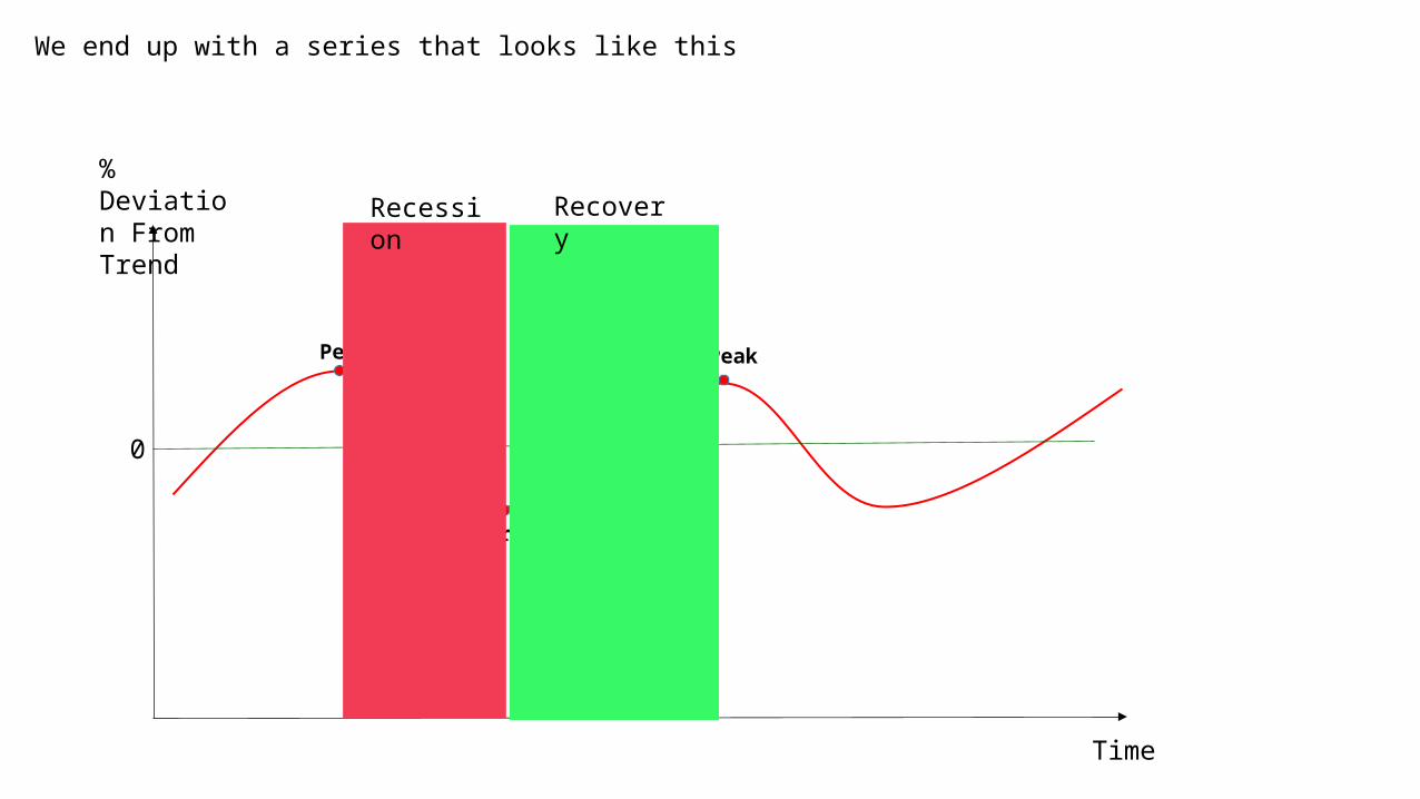
We end up with a series that looks like this
% Deviation From Trend
Time
0
Trough
Peak Peak
Recession Recovery

1/1/1919 1/1/1939 1/1/1959 1/1/1979 1/1/1999
-40
-30
-20
-10
0
10
20
30
Great Depression WWII
We have had 22 full cycles since 1900.%
Dev
iatio
n fr
om tr
end
Indu
stria
l Pro
ducti
on
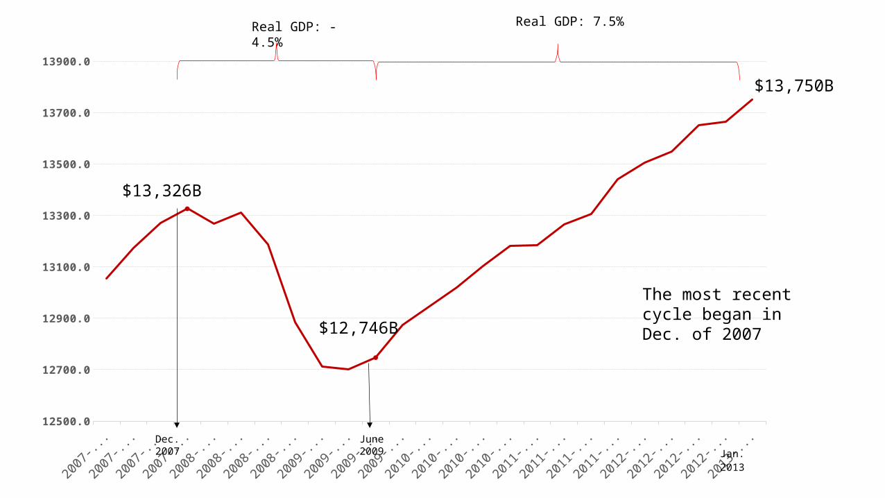
2007-01-01 2009-01-01 2011-01-01 2013-01-0112500.0
12700.0
12900.0
13100.0
13300.0
13500.0
13700.0
13900.0
Jan. 2013
$13,326B
$12,746B
$13,750B
Real GDP: -4.5% Real GDP: 7.5%
Dec. 2007 June 2009
The most recent cycle began in Dec. of 2007

2007-01-01 2009-01-01 2011-01-01 2013-01-01
-4
-3
-2
-1
0
1
2
3
Recession Recovery
% D
evia
tion
from
tren
d G
DP
Dec. 2007“Peak”
June 2009“Trough”
2.5%
-2.8%
The most recent cycle in terms of deviation from trend
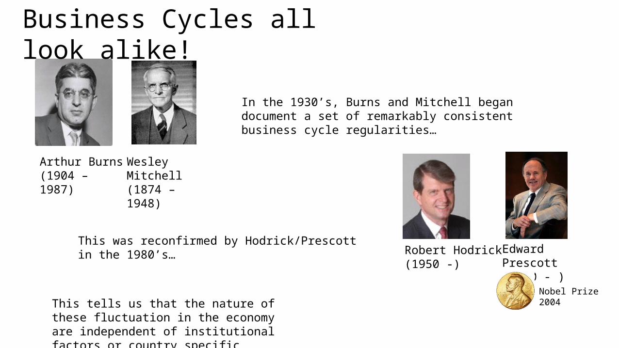
Arthur Burns(1904 – 1987)
Wesley Mitchell(1874 – 1948)
Robert Hodrick(1950 -)
Edward Prescott(1940 - )
Business Cycles all look alike!
In the 1930’s, Burns and Mitchell began document a set of remarkably consistent business cycle regularities…
This was reconfirmed by Hodrick/Prescott in the 1980’s…
This tells us that the nature of these fluctuation in the economy are independent of institutional factors or country specific issues!!
Nobel Prize 2004

By “regularities”, we are referring to statistical relationships….
Time
GDP
Time
GDP
X
X
Time
GDP
X
Procyclical variables move in the same direction as GDP
Countercyclical variables move in the opposite direction as GDP
Acyclical variables have no obvious relationship to GDP
CORR(GDP, X) >0
CORR(GDP, X) <0
CORR(GDP, X) =0
Peak
Trough
Indu
stria
l Pro
ducti
on (%
Dev
iatio
n fr
om T
rend
)
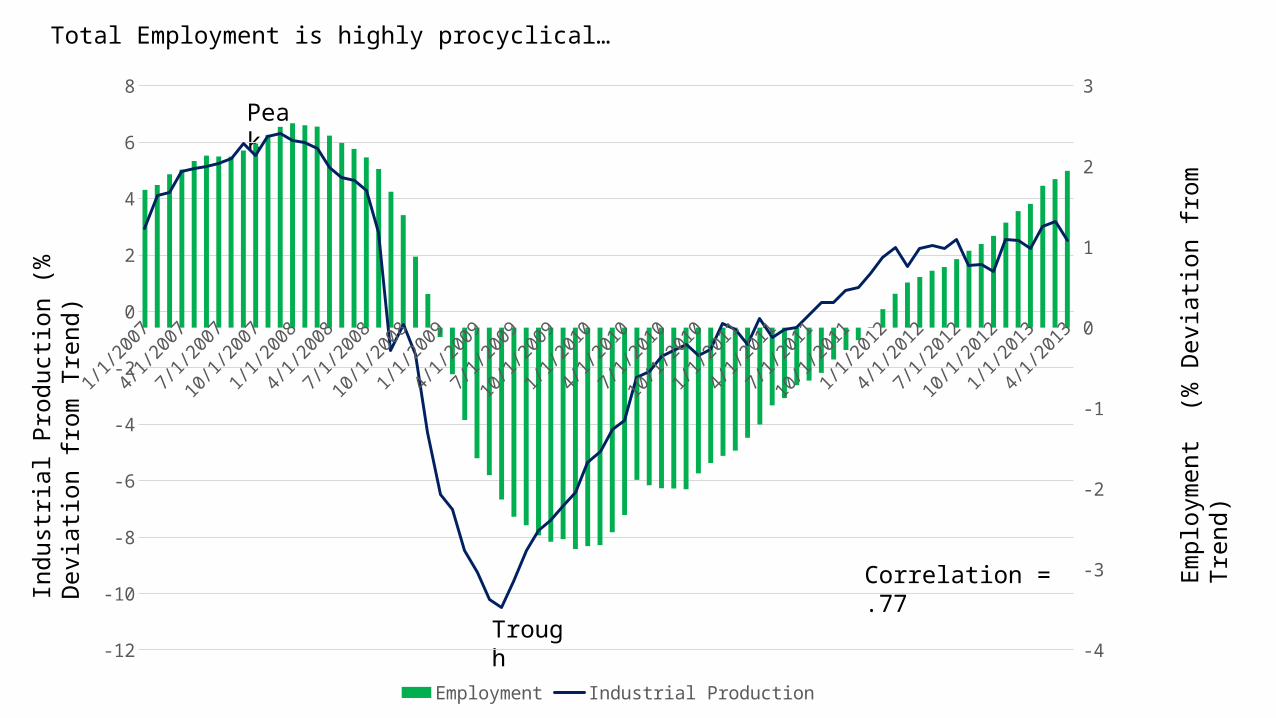
Correlation = .77
1/1/2007 1/1/2009 1/1/2011 1/1/2013
-12
-10
-8
-6
-4
-2
0
2
4
6
8
-4
-3
-2
-1
0
1
2
3
Employment Industrial Production
Empl
oym
ent
(% D
evia
tion
from
Tre
nd)
Total Employment is highly procyclical…

1/1/2007 1/1/2009 1/1/2011 1/1/2013
-12
-10
-8
-6
-4
-2
0
2
4
6
8
4
5
6
7
8
9
10
11
Unemployment Rate Industrial Production
Indu
stria
l Pro
ducti
on (%
Dev
iatio
n fr
om T
rend
)
Une
mpl
oym
ent R
ate
Peak
Trough
5%
9.5%
Correlation = -.54
Therefore, the unemployment rate will be countercyclical!
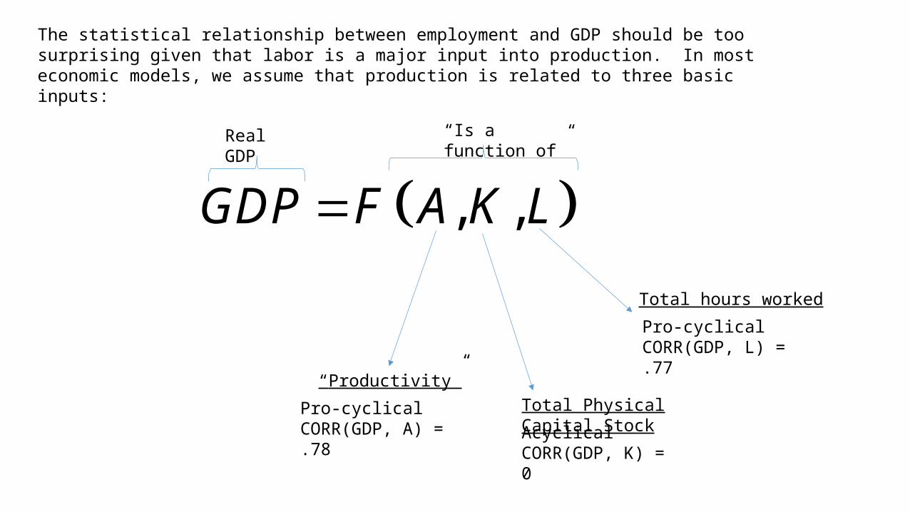
The statistical relationship between employment and GDP should be too surprising given that labor is a major input into production. In most economic models, we assume that production is related to three basic inputs:
, ,GDP F A K L
Real GDP “Is a function of”
Total hours worked
Total Physical Capital Stock“Productivity”
Pro-cyclicalCORR(GDP, A) = .78
Pro-cyclicalCORR(GDP, L) = .77
AcyclicalCORR(GDP, K) = 0
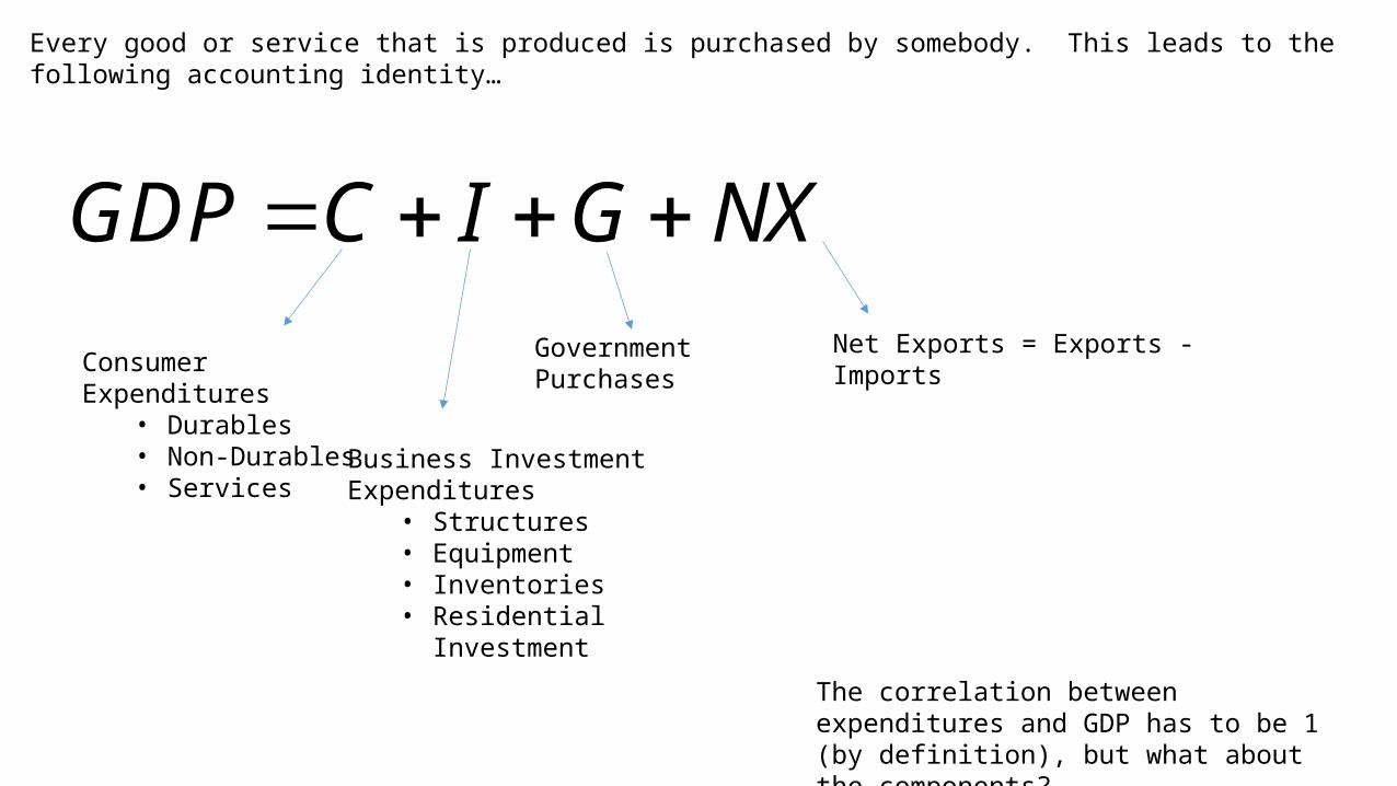
Every good or service that is produced is purchased by somebody. This leads to the following accounting identity…
GDP C I G NX Consumer Expenditures
• Durables• Non-Durables• Services Business Investment
Expenditures• Structures• Equipment• Inventories• Residential
Investment
Government Purchases Net Exports = Exports - Imports
The correlation between expenditures and GDP has to be 1 (by definition), but what about the components?

7/1/2007 7/1/2009 7/1/2011
-12
-10
-8
-6
-4
-2
0
2
4
6
8
Retail Sales Industrial Production
% D
evia
tion
from
Tre
nd
Peak
Trough Correlation = .82
Retail sales is essentially the goods portion of consumer expenditures (durables and non-durables)
2007-01-01 2009-01-01 2011-01-01 2013-01-01
-4
-3
-2
-1
0
1
2
3
4
Consumption GDP
GD
P (D
evia
tion
from
Tre
nd)
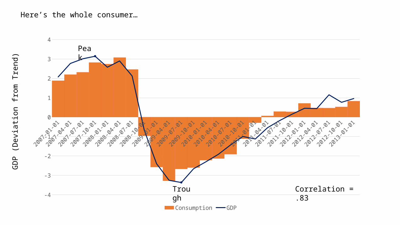
Correlation = .83Trough
Peak
Here’s the whole consumer…
2007-01-01 2009-01-01 2011-01-01 2013-01-01
-25
-20
-15
-10
-5
0
5
10
15
Gross Investment GDP
% D
evia
tion
from
Tre
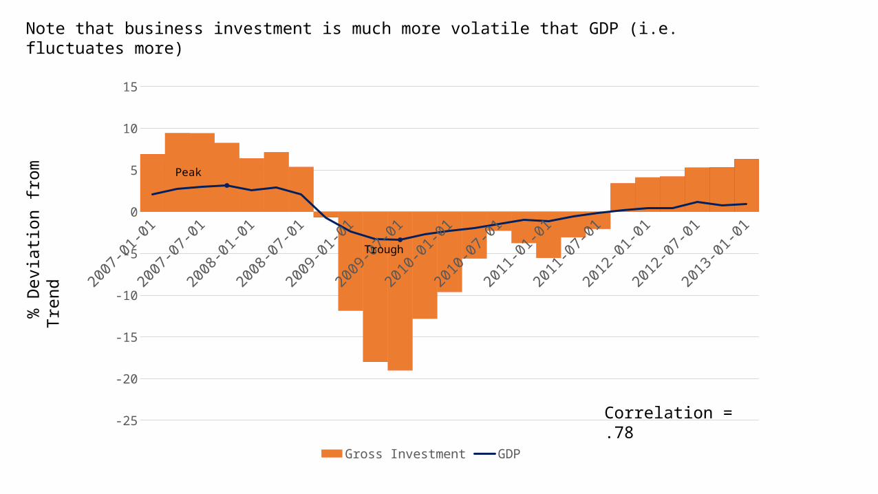
nd Peak
Trough
Correlation = .78
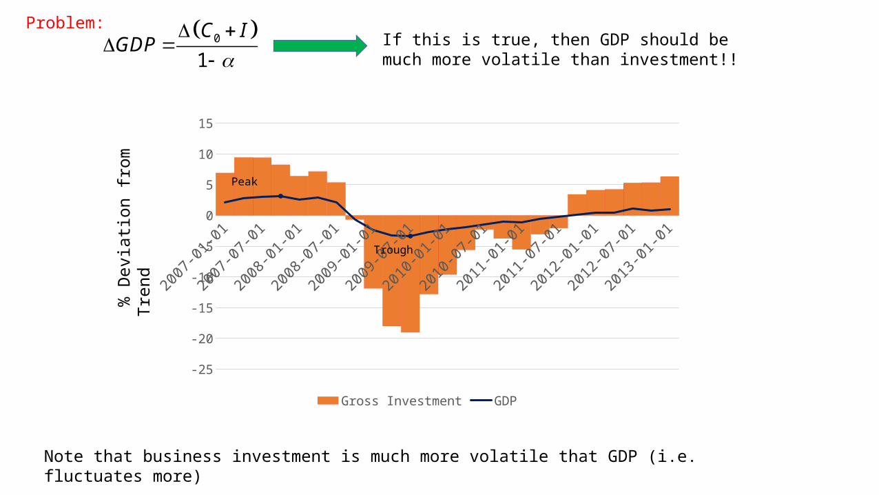
Note that business investment is much more volatile that GDP (i.e. fluctuates more)
2007-01-01 2009-01-01 2011-01-01 2013-01-01
-6
-4
-2
0
2
4
6
Government Expenditures GDP
% D
evia
tion
from
Tre
nd
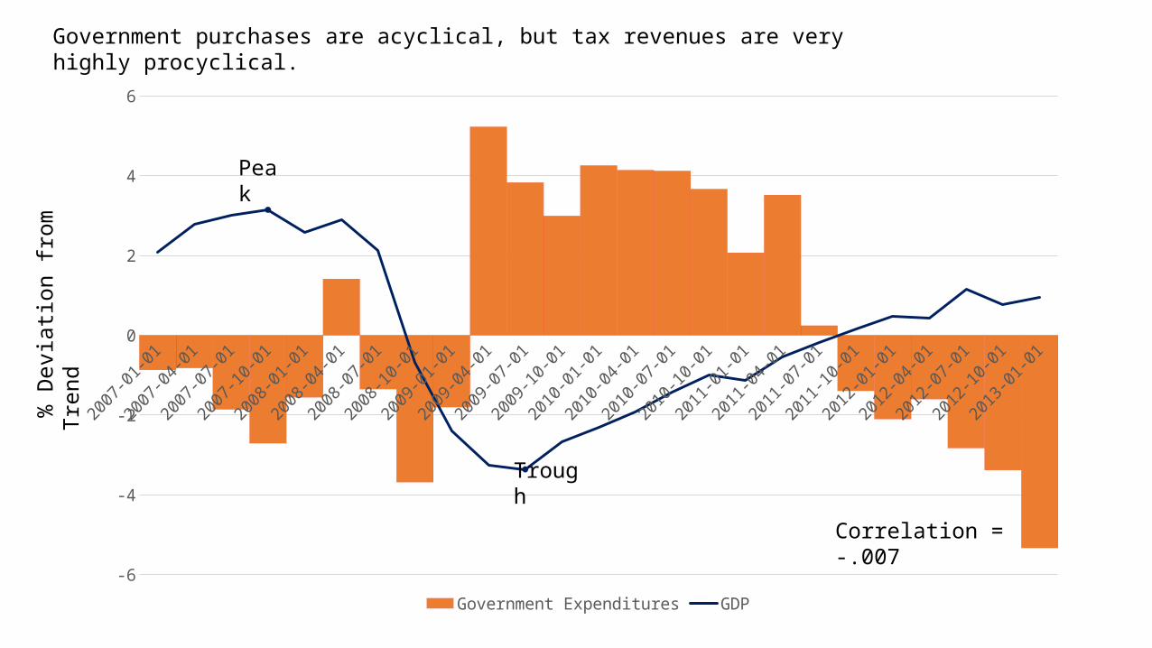
Peak
Trough
Correlation = -.007
Government purchases are acyclical, but tax revenues are very highly procyclical.
2006-07-01 2008-07-01 2010-07-01 2012-07-01
-4
-3
-2
-1
0
1
2
3
4
-150
-100
-50
0
50
100
150
200
250
300
Trade Balance GDP
GD
P (D
evia
tion
from
Tre
nd)
Trad
e Ba
lanc
e (D
iffer
ence
from
Tre
nd B
illio
ns o
f Dol
lars
)
Peak
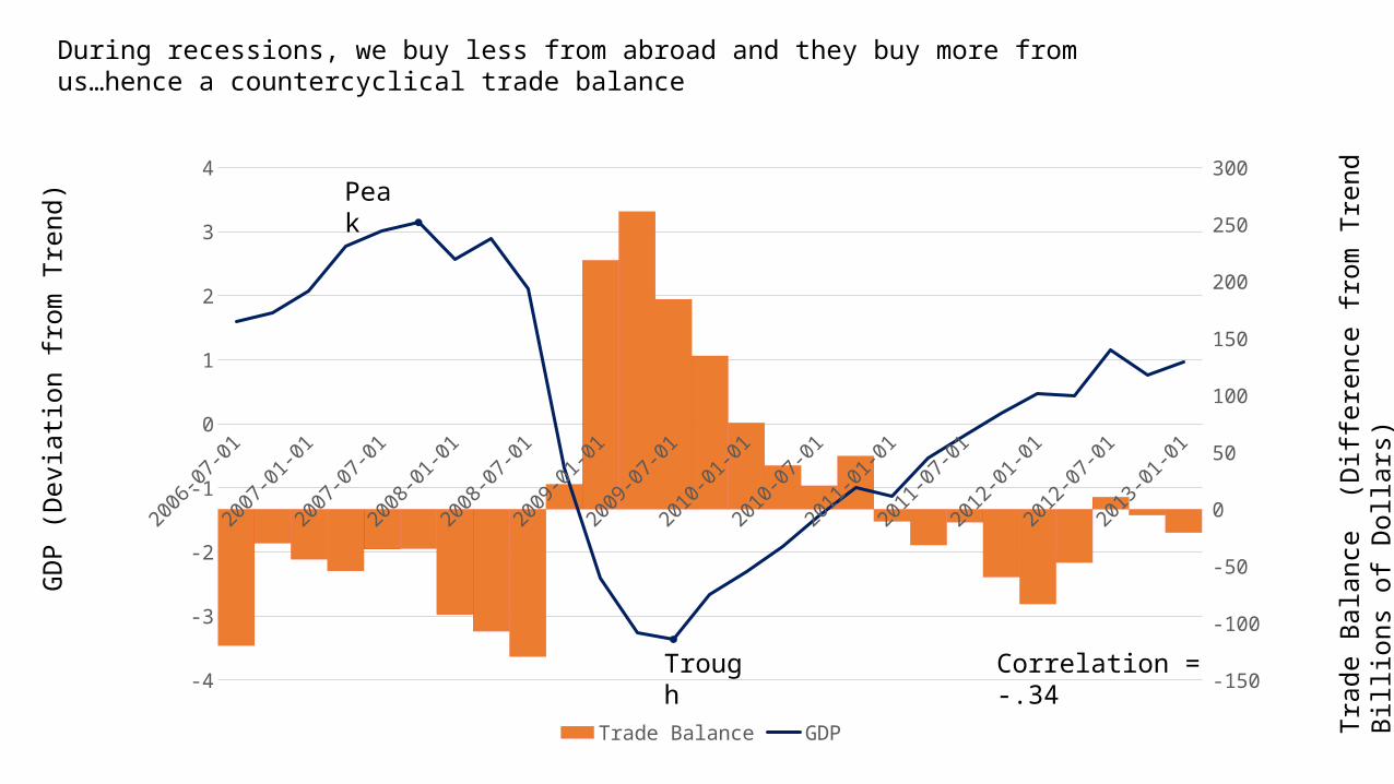
Trough Correlation = -.34
During recessions, we buy less from abroad and they buy more from us…hence a countercyclical trade balance
2007-01-01 2009-01-01 2011-01-01 2013-01-01
-4
-3
-2
-1
0
1
2
3
Real Wages Real GDP
Trough
Peak
Dev
iatio
n fr
om T
rend
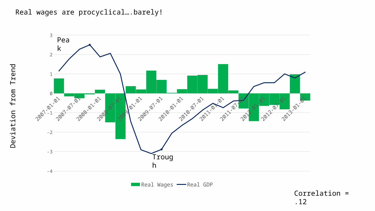
Correlation = .12
Real wages are procyclical….barely!
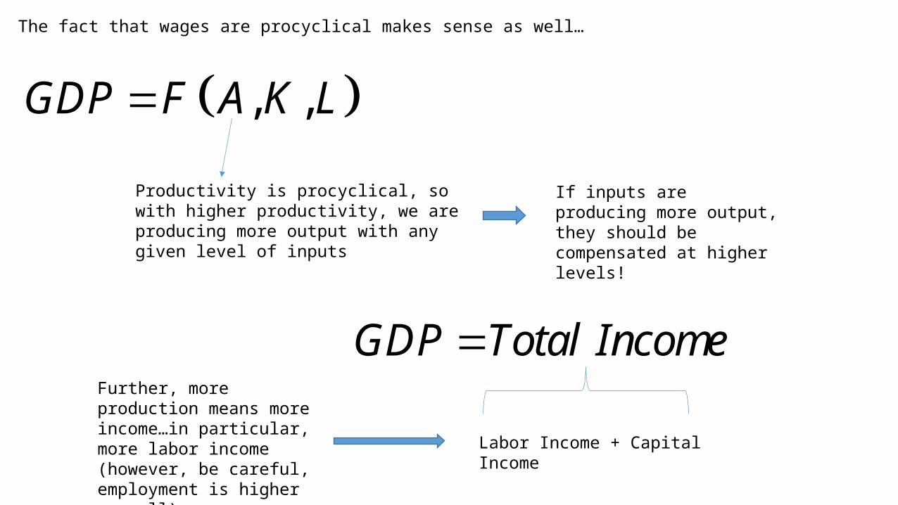
The fact that wages are procyclical makes sense as well…
, ,GDP F A K L
Productivity is procyclical, so with higher productivity, we are producing more output with any given level of inputs
GDP Total Income
Labor Income + Capital Income
If inputs are producing more output, they should be compensated at higher levels!
Further, more production means more income…in particular, more labor income (however, be careful, employment is higher as well)
2007-01-01 2009-01-01 2011-01-01 2013-01-01
-4
-3
-2
-1
0
1
2
3
Price Real GDP
% D
evia
tion
from
tren
d G
DP
% D
evia
tion
from
tren
d Pr
ice
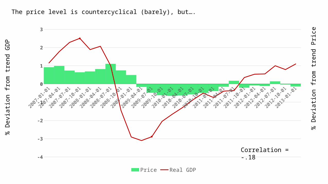
Correlation = -.18
The price level is countercyclical (barely), but….
2007-01-01 2009-01-01 2011-01-01 2013-01-01
-4
-3
-2
-1
0
1
2
3
4
5
Inflation Real GDP
Annu
al In
flatio
n Ra
te
Real
GD
P (D
evia
tion
from
Tre
nd)
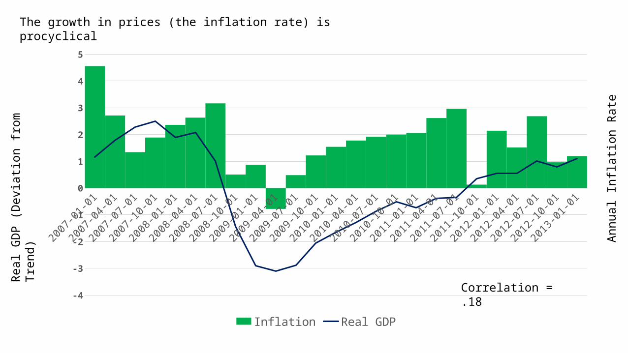
Correlation = .18
The growth in prices (the inflation rate) is procyclical
1/1/2007 1/1/2009 1/1/2011 1/1/2013
-12
-10
-8
-6
-4
-2
0
2
4
6
8
0
1
2
3
4
5
6
1 Year Treasury Rate Industrial Production
Peak
Trough
Indu
stria
l Pro
ducti
on (%
Dev
iatio
n fr
om T
rend
)
1 Ye
ar T
reas
ury
Rate
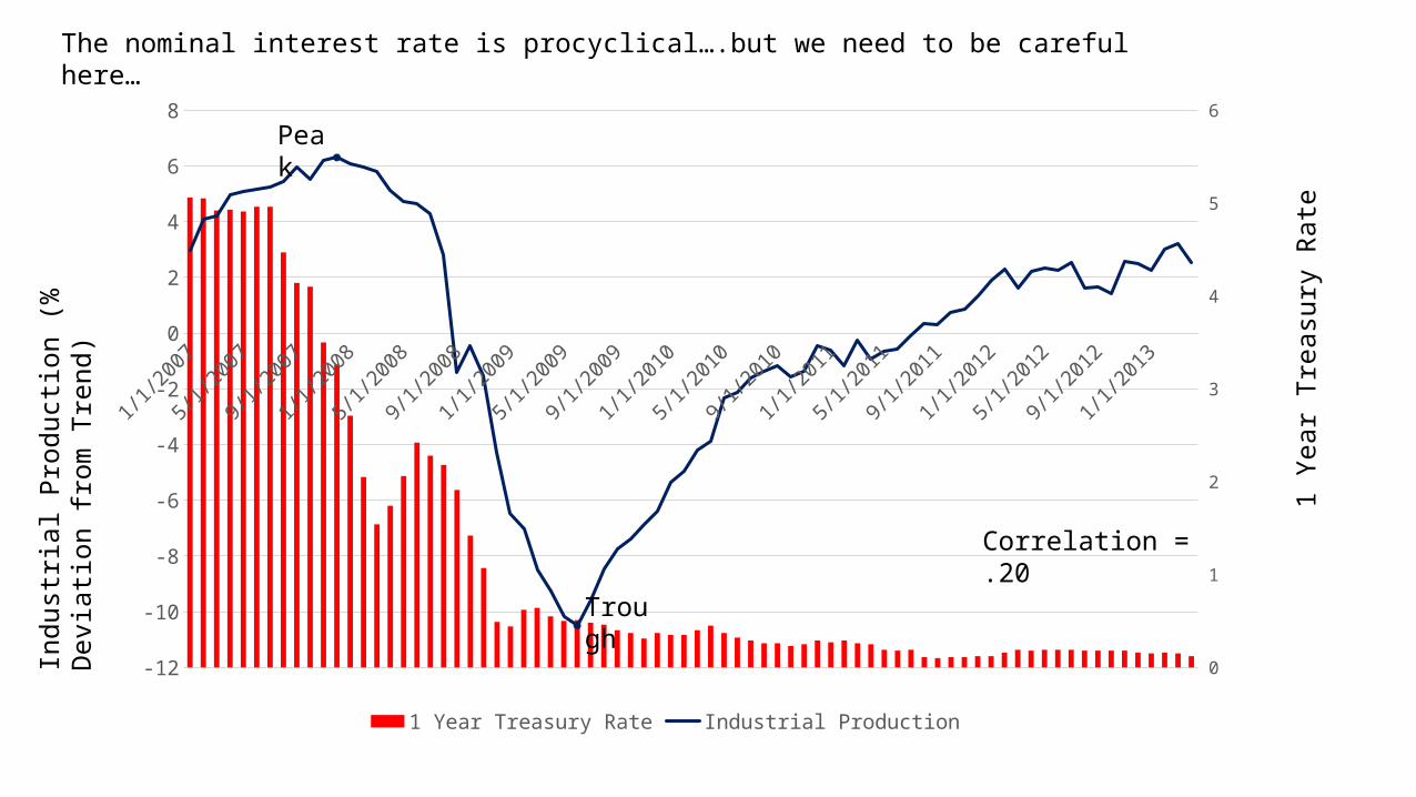
Correlation = .20
The nominal interest rate is procyclical….but we need to be careful here…
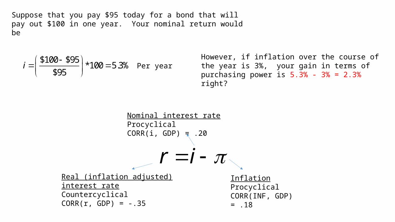
Suppose that you pay $95 today for a bond that will pay out $100 in one year. Your nominal return would be
$100 $95*100 5.3%
$95i
Per yearHowever, if inflation over the course of the year is 3%, your gain in terms of purchasing power is 5.3% - 3% = 2.3% right?
r i Real (inflation adjusted) interest rateCountercyclicalCORR(r, GDP) = -.35
Nominal interest rateProcyclicalCORR(i, GDP) = .20
InflationProcyclicalCORR(INF, GDP) = .18
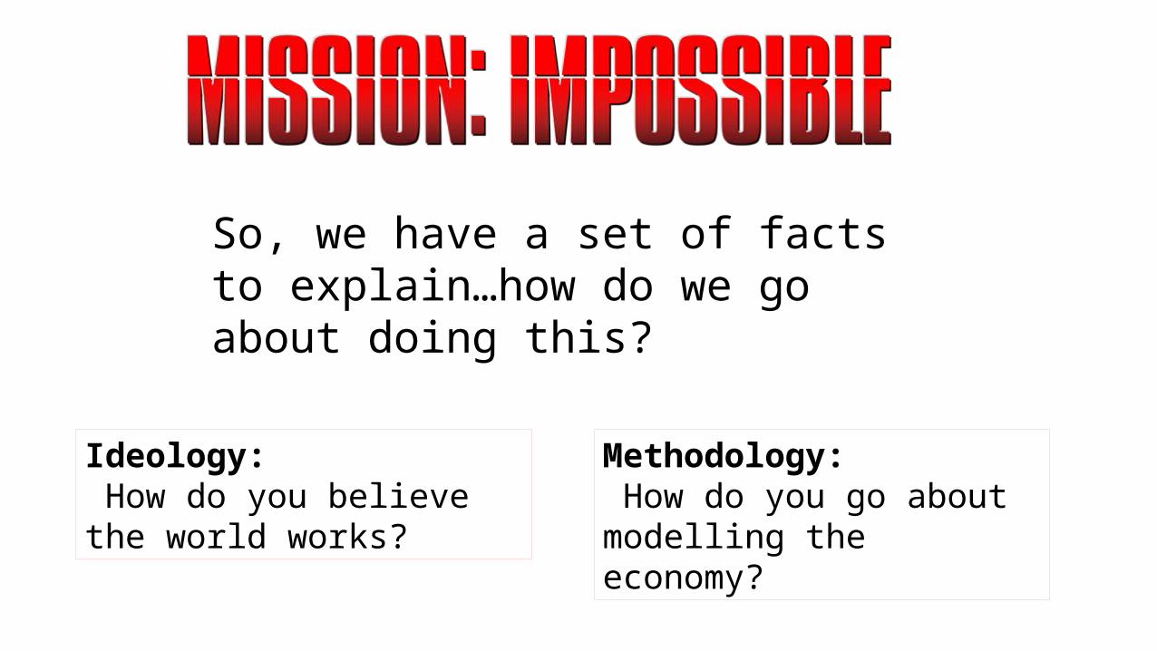
So, we have a set of facts to explain…how do we go about doing this?
Ideology: How do you believe the world works?
Methodology: How do you go about modelling the economy?

Say's law states that the production of goods creates its own demand. In 1803, John Baptiste Say explained his theory. This view suggests that the key to economic growth is not increasing demand, but increasing production.
Jean-Baptiste Say (1767 -1832)
Classical Economics
Adam Smith (1723 – 1790) David Ricardo (1772 – 1823) Thomas Malthus (1766 – 1834) John Stuart Mill (1806 – 1873)
It should be noted that while classical economists were aware of what was called at the time the “Boom Bust cycle”, they weren’t overly concerned about it and focused primarily on microeconomic issues.

John Maynard Keynes (1883 – 1946)
"I believe myself to be writing a book on economic theory which will largely revolutionize—not I suppose, at once but in the course of the next ten years—the way the world thinks about its economic problems. I can't expect you, or anyone else, to believe this at the present stage. But for myself I don't merely hope what I say,--in my own mind, I'm quite sure."
The General Theory of Employment, Interest and Money (1936)
Keynesian Economics is the view that in the short run, especially during recessions, economic output is strongly influenced by aggregate demand (total spending in the economy). In the Keynesian view, aggregate demand does not necessarily equal the productive capacity of the economy; instead, it is influenced by a host of factors and sometimes behaves erratically, affecting production, employment, and inflation.
*Note: The Nobel prize in economics was first awarded in 1969. The statutes of the Nobel Foundation stipulate that the prize cannot be awarded posthumously.

Consider, for simplicity, an economy with no government that does not trade with the rest of the world…
t tGDP C I
Suppose that, investment in this economy increases by $100
t tGDP C I
The $100 investment generates $100 increase in GDP
+$100+$100
So, what happens next?
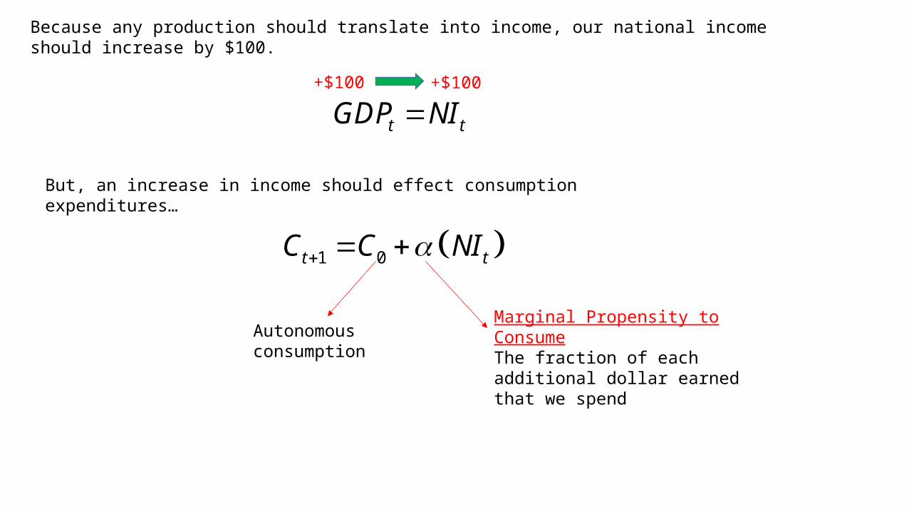
Because any production should translate into income, our national income should increase by $100.
t tGDP NI
But, an increase in income should effect consumption expenditures…
1 0t tC C NI
Autonomous consumption
Marginal Propensity to ConsumeThe fraction of each additional dollar earned that we spend
+$100+$100
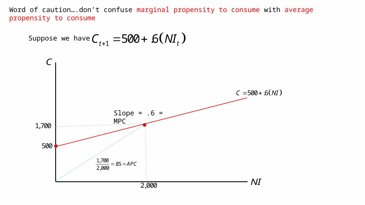
Word of caution….don’t confuse marginal propensity to consume with average propensity to consume
1 500 .6t tC NI Suppose we have
C
NI
500
500 .6C NI
Slope = .6 = MPC
2,000
1,700
1,700.85
2,000APC
1 0t tC C NI
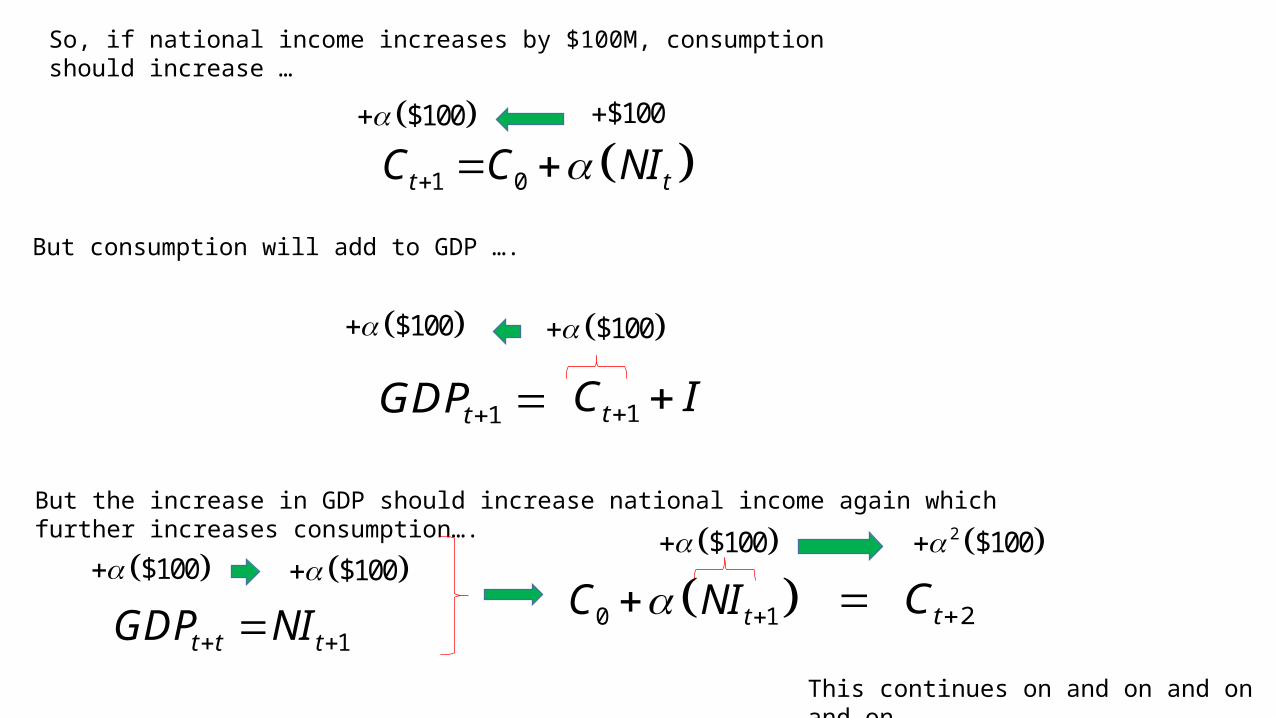
So, if national income increases by $100M, consumption should increase …
$100 $100
But consumption will add to GDP ….
1tC I
$100 $100
1tGDP
But the increase in GDP should increase national income again which further increases consumption….
1t t tGDP NI $100 $100
0 1tC NI $100
2tC
2 $100
This continues on and on and on and on…
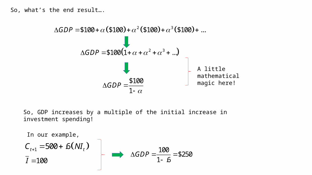
So, what’s the end result….
2 3$100 $100 $100 $100 ...GDP
2 3$100 1 ...GDP
$100
1GDP
A little mathematical magic here!
So, GDP increases by a multiple of the initial increase in investment spending!
In our example,
100$250
1 .6GDP
100I
1 500 .6t tC NI
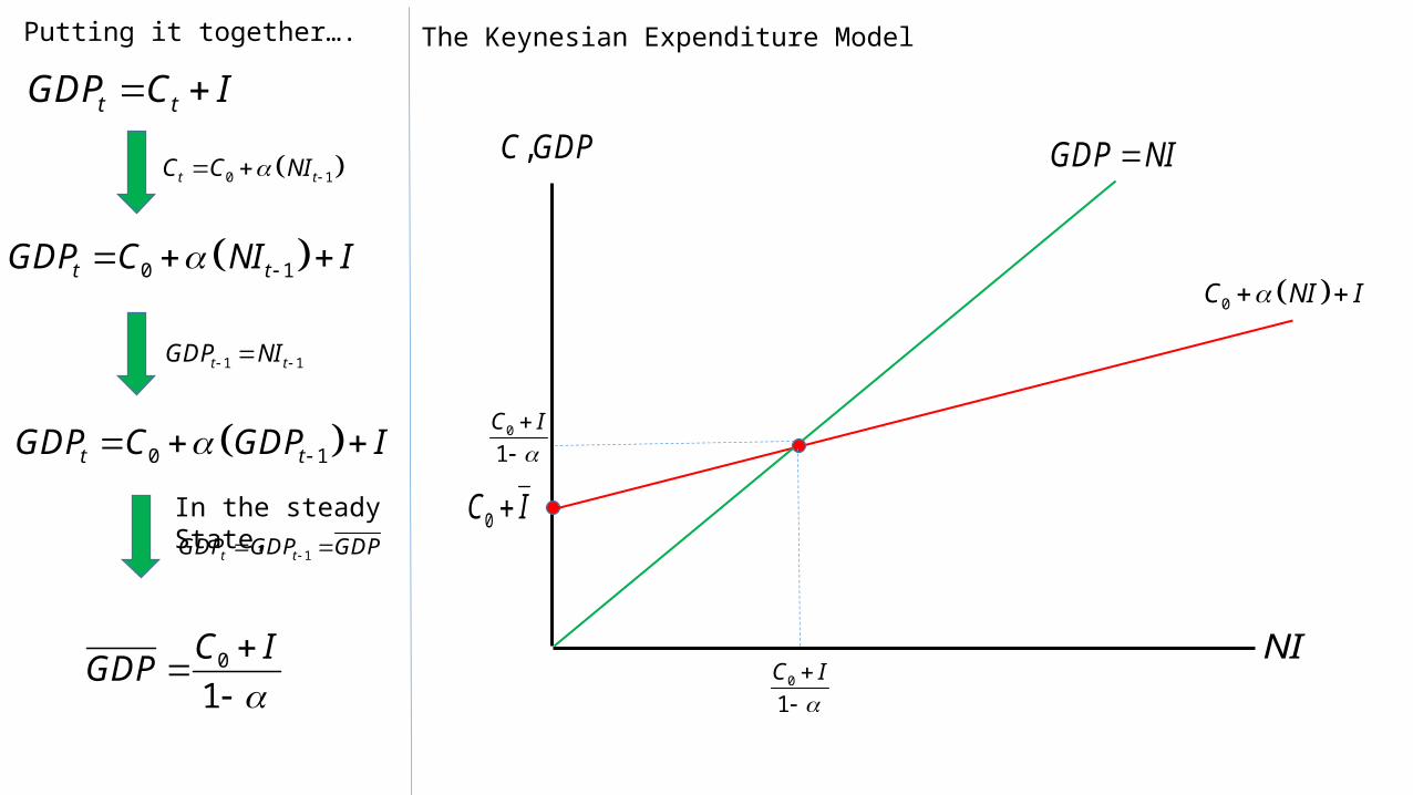
Putting it together….
t tGDP C I
0 1t tC C NI
0 1t tGDP C NI I
1 1t tGDP NI
0 1t tGDP C GDP I
In the steady State,
0
1
C IGDP
,C GDP
NI
0C NI I
GDP NI
0C I
0
1
C I
0
1
C I
The Keynesian Expenditure Model
1t tGDP GDP GDP
,C GDP
NI
0C NI I
GDP NI
600
1,500
1,500
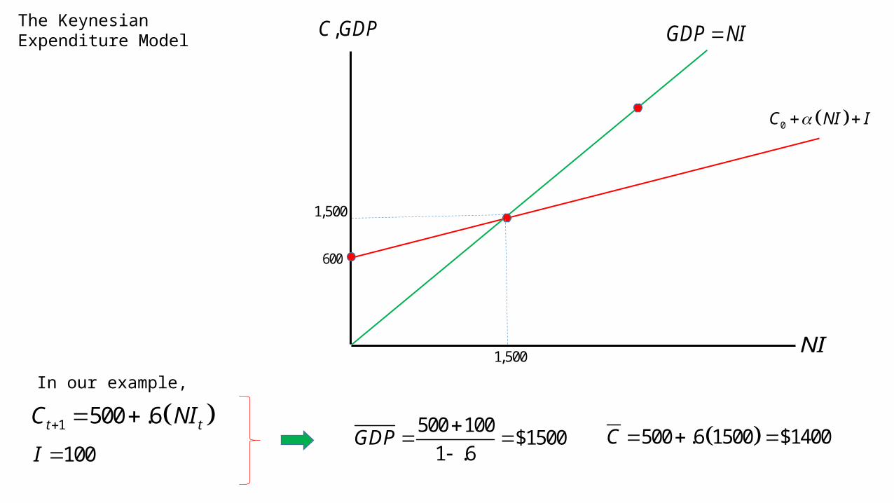
The Keynesian Expenditure Model
In our example,
500 100$1500
1 .6GDP
100I
1 500 .6t tC NI 500 .6 1500 $1400C
,C GDP
NI
0C NI I
GDP NI
600
1,500
1,500
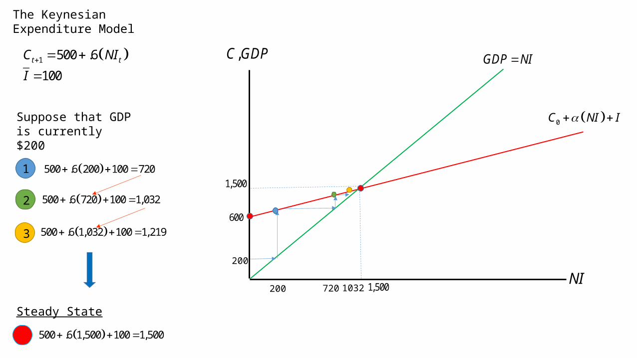
The Keynesian Expenditure Model
Suppose that GDP is currently $200
200
200
100I 1 500 .6t tC NI
500 .6 200 100 720
720
500 .6 720 100 1,032
1032
500 .6 1,032 100 1,219
1
2
3
500 .6 1,500 100 1,500
Steady State
Time 1 2 3 4 5 6 7 8 9 10 110
200
400
600
800
1000
1200
1400
1600
YC
I
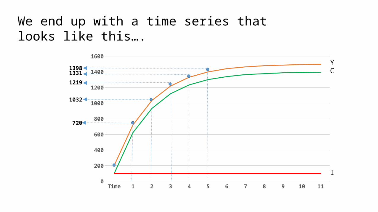
We end up with a time series that looks like this….
720
1032
1219
13311398
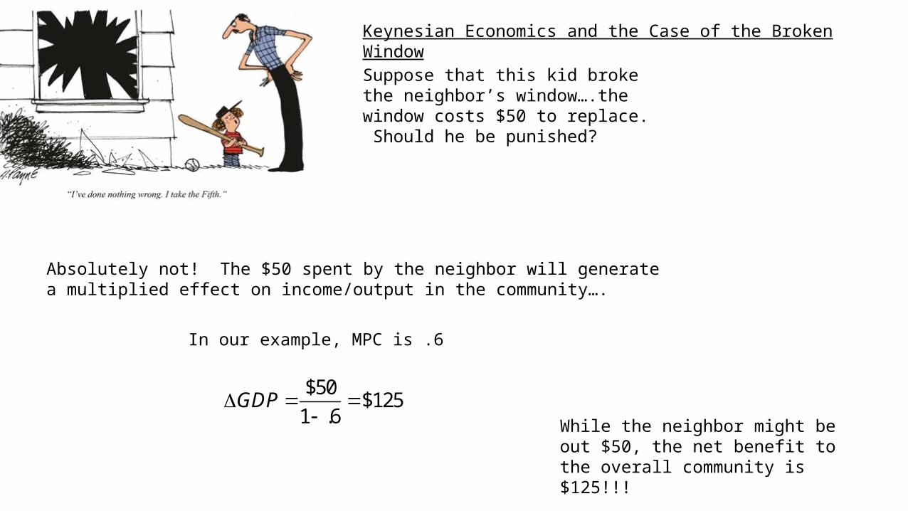
Suppose that this kid broke the neighbor’s window….the window costs $50 to replace. Should he be punished?
Absolutely not! The $50 spent by the neighbor will generate a multiplied effect on income/output in the community….
Keynesian Economics and the Case of the Broken Window
$50$125
1 .6GDP
In our example, MPC is .6
While the neighbor might be out $50, the net benefit to the overall community is $125!!!

,C GDP
NI
0GDP C NI I
GDP NI
0C I
*GDP
*NI
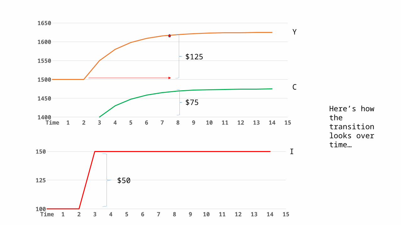
So, if investment expenditures rise by $50…
$50
$50$50
$1251 .6
GDP
$50$125
1 .6NI
Time 1 2 3 4 5 6 7 8 9 10 11 12 13 14 151400
1450
1500
1550
1600
1650
Time 1 2 3 4 5 6 7 8 9 10 11 12 13 14 15100
125
150
Y
C
I
$125
$50
Here’s how the transition looks over time…
$75
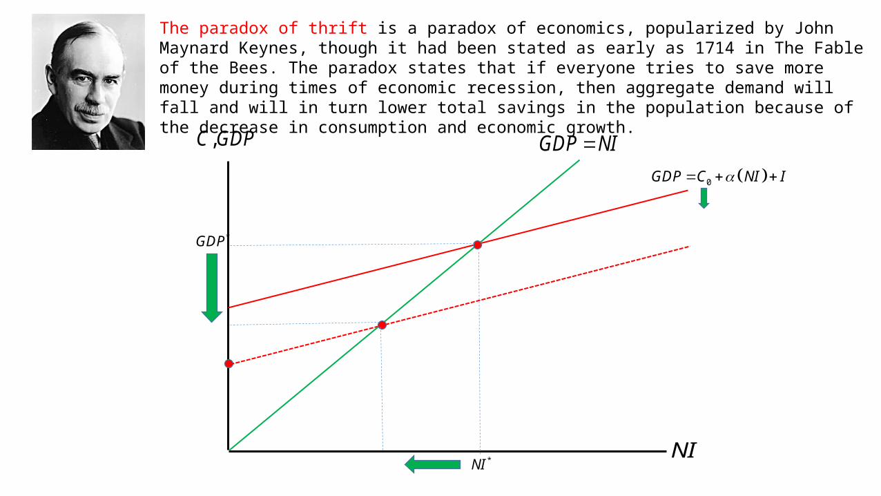
The paradox of thrift is a paradox of economics, popularized by John Maynard Keynes, though it had been stated as early as 1714 in The Fable of the Bees. The paradox states that if everyone tries to save more money during times of economic recession, then aggregate demand will fall and will in turn lower total savings in the population because of the decrease in consumption and economic growth.
,C GDP
NI
0GDP C NI I
GDP NI
*GDP
*NI
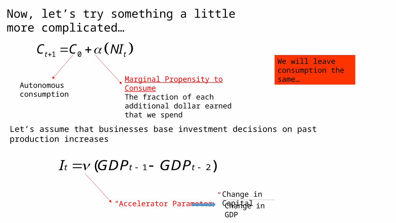
Now, let’s try something a little more complicated…
1 0t tC C NI
Autonomous consumption
Marginal Propensity to ConsumeThe fraction of each additional dollar earned that we spend
We will leave consumption the same…
Let’s assume that businesses base investment decisions on past production increases
1 2( )t t tI GDP GDP
“Accelerator Parameter”Change in Capital
Change in GDP
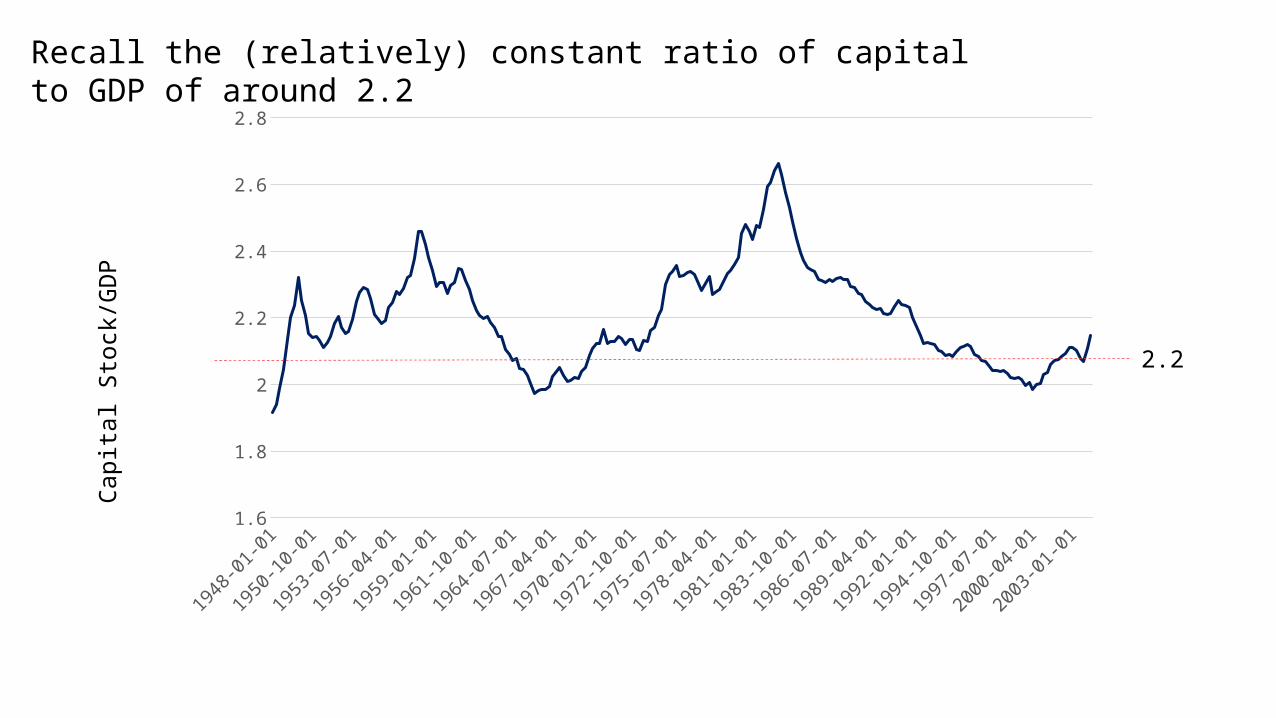
1948 1963 1978 19931.6
1.8
2
2.2
2.4
2.6
2.8
2.2
Recall the (relatively) constant ratio of capital to GDP of around 2.2
Capi
tal S
tock
/GD
P
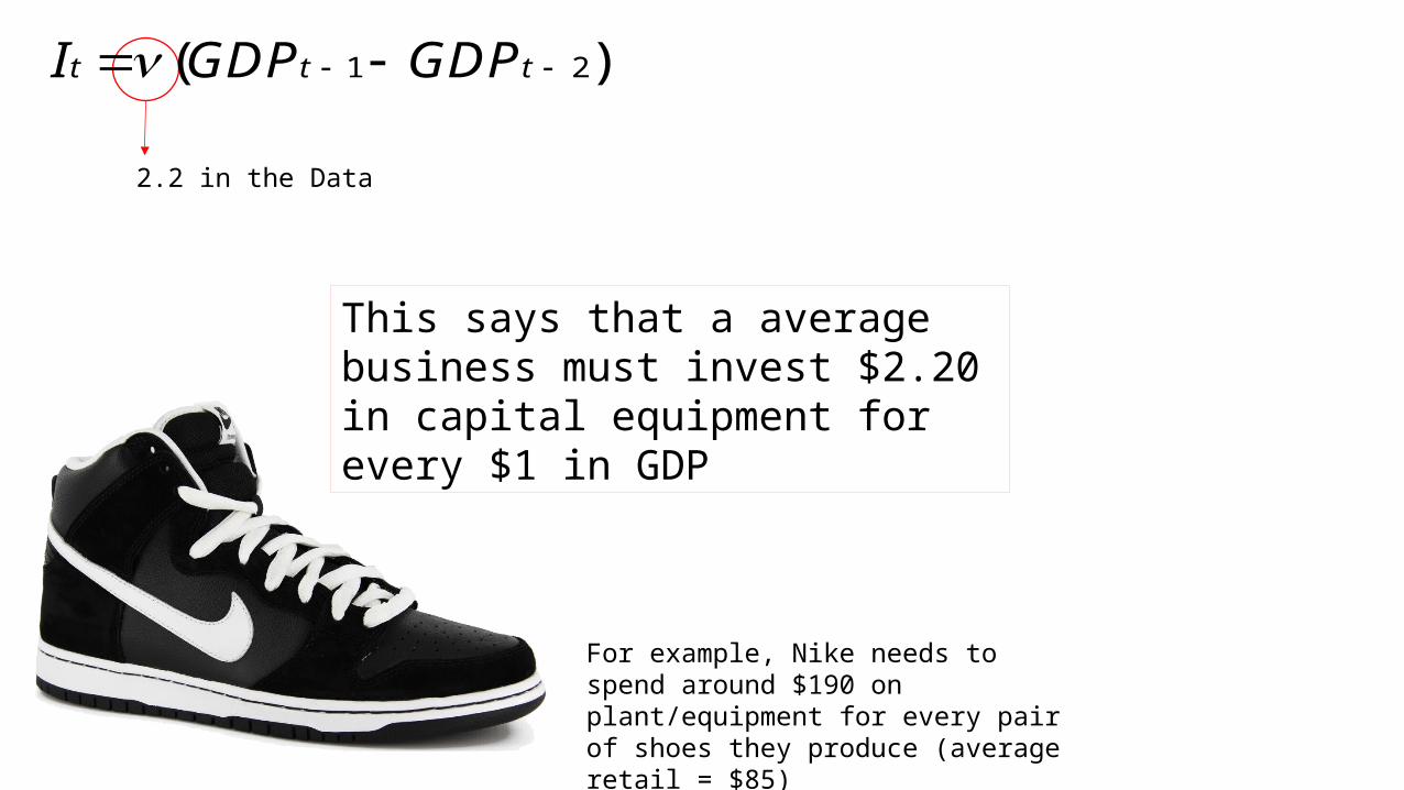
1 2( )t t tI GDP GDP
2.2 in the Data
This says that a average business must invest $2.20 in capital equipment for every $1 in GDP
For example, Nike needs to spend around $190 on plant/equipment for every pair of shoes they produce (average retail = $85)

t t tGDP C I
0t tC C NI
t tGDP NI
0 1 1 2t t t tGDP C GDP GDP GDP
0
1
CGDP
1t tGDP GDP GDP
Putting everything together….
1 2( )t t tI GDP GDP
0 1 2t t tGDP C GDP vGDP
In the Steady State, GDP is constant
In the steady state, GDP is constant (and, hence, investment is zero)
tC tI

500 .6t tC NI
t tGDP NI
1 2( )t t tI GDP GDP
Let’s Suppose the following
Same as before
Let the accelerator parameter equal 1
We need two initial values for GDP to get started….
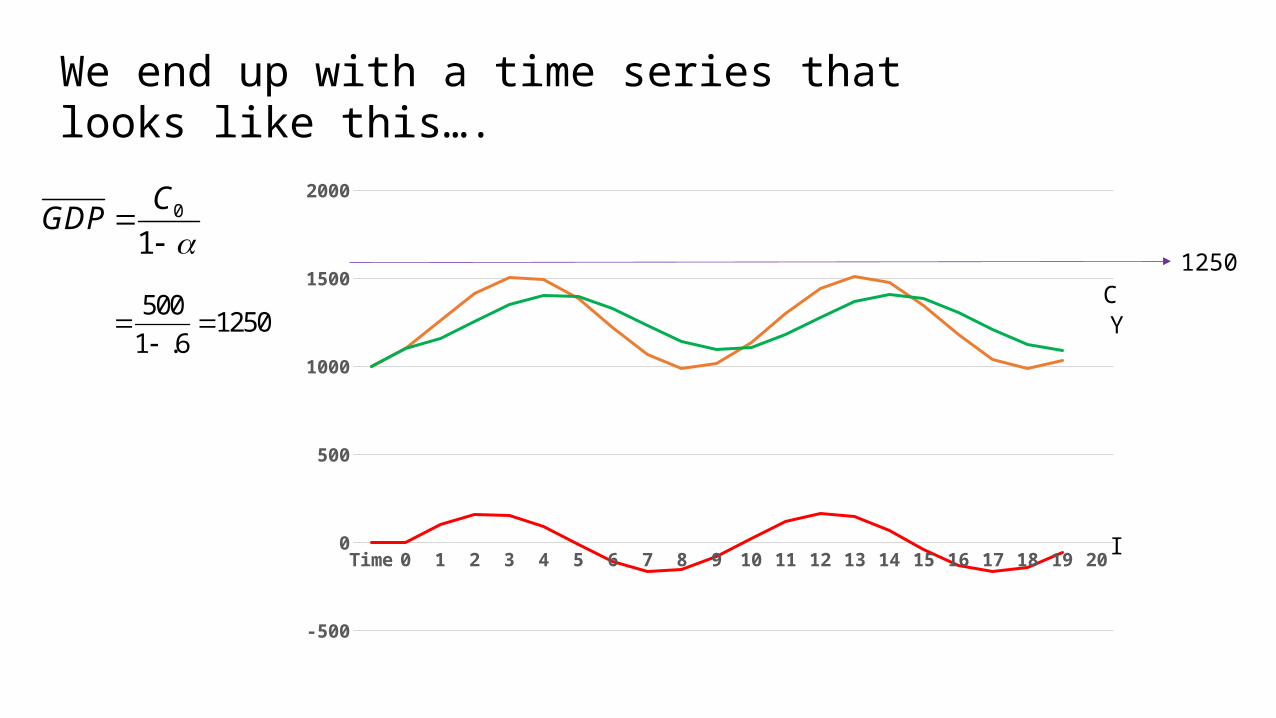
0 5001250
1 1 .6
CGDP
Time GDP Consumption Investment
0 1000
1 1100 1100
2 1260 1160 100
3 1416 1256 160
4 1505.6 1349.6 156
1500 .6t tC GDP 1 2( )t t tI GDP GDP
1 2500 1.6t t tGDP GDP GDP
Time
0 1 2 3 4 5 6 7 8 9 10 11 12 13 14 15 16 17 18 19 20
-500
0
500
1000
1500
2000
YC
I
We end up with a time series that looks like this….
0
1
CGDP
5001250
1 .6
1250
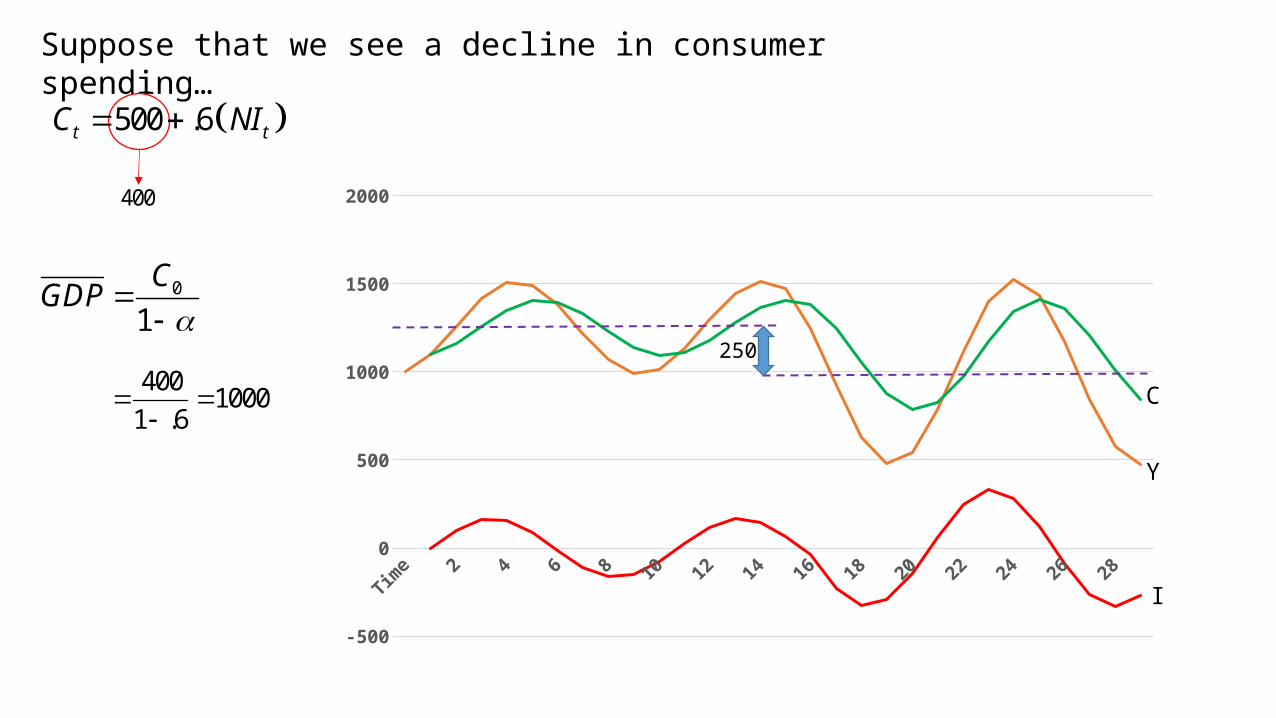
Suppose that we see a decline in consumer spending…
500 .6t tC NI
400
Time
1 2 3 4 5 6 7 8 9 10 11 12 13 14 15 16 17 18 19 20 21 22 23 24 25 26 27 28 29
-500
0
500
1000
1500
2000
0
1
CGDP
4001000
1 .6
250
Y
C
I
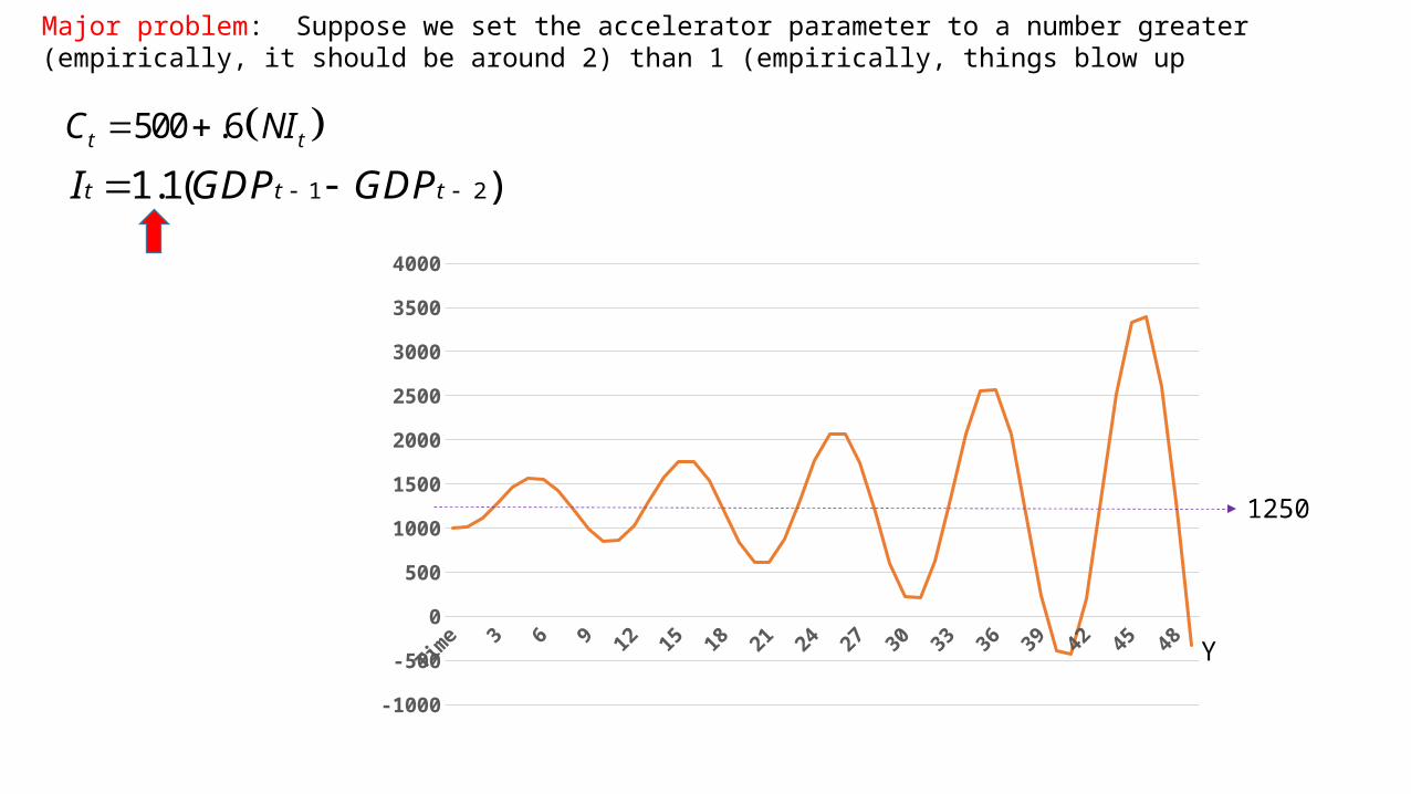
Major problem: Suppose we set the accelerator parameter to a number greater (empirically, it should be around 2) than 1 (empirically, things blow up
500 .6t tC NI
1 21.1( )t t tI GDP GDP
Time 2 4 6 8 10 12 14 16 18 20 22 24 26 28 30 32 34 36 38 40 42 44 46 48
-1000
-500
0
500
1000
1500
2000
2500
3000
3500
4000
Y
1250
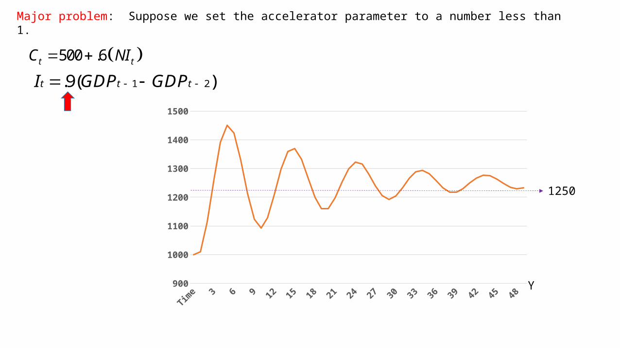
Major problem: Suppose we set the accelerator parameter to a number less than 1.
500 .6t tC NI
1 2.9( )t t tI GDP GDP
Time 2 4 6 8 10 12 14 16 18 20 22 24 26 28 30 32 34 36 38 40 42 44 46 48
900
1000
1100
1200
1300
1400
1500
Y
1250

Keynesian Economics
Fundamental belief: The economy is demand driven. The business cycle is a result of random fluctuations is spending behavior (“Animal Spirits”)
GDP C I
Modelling Strategy: Use macroeconomic data and time series analysis to develop relationships between macroeconomic variables
2007-01-01 2009-01-01 2011-01-01 2013-01-01
-25
-20
-15
-10
-5
0
5
10
15
Gross Investment GDP
% D
evia
tion
from
Tre
nd
Peak
Trough
Note that business investment is much more volatile that GDP (i.e. fluctuates more)
Problem: 0
1
C IGDP
If this is true, then GDP should be much more volatile than investment!!

GDP C I
Problem: Keynesian economics suggests that GDP responds to changes in demand. If demand goes up, where does this extra production come from?
If aggregate demand exceeds supply (i.e. we are trying to buy more goods than are available) what happens?
• In an open economy, the trade deficit worsens (we get the extra goods from overseas.
• In a closed economy, the interest rate rises (higher interest rates should discourage spending)
Neither of these effects are mentioned!!!!

Have you ever heard the story about the economist and the NFL?
Typical Economist
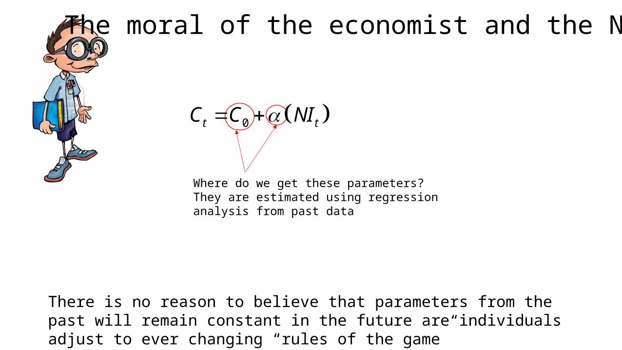
0t tC C NI
Where do we get these parameters? They are estimated using regression analysis from past data
The moral of the economist and the NFL
There is no reason to believe that parameters from the past will remain constant in the future are individuals adjust to ever changing “rules of the game”
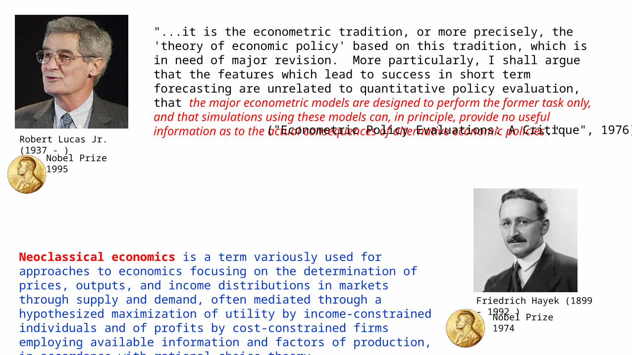
Robert Lucas Jr. (1937 - )
Nobel Prize 1995
Neoclassical economics is a term variously used for approaches to economics focusing on the determination of prices, outputs, and income distributions in markets through supply and demand, often mediated through a hypothesized maximization of utility by income-constrained individuals and of profits by cost-constrained firms employing available information and factors of production, in accordance with rational choice theory
"...it is the econometric tradition, or more precisely, the 'theory of economic policy' based on this tradition, which is in need of major revision. More particularly, I shall argue that the features which lead to success in short term forecasting are unrelated to quantitative policy evaluation, that the major econometric models are designed to perform the former task only, and that simulations using these models can, in principle, provide no useful information as to the actual consequences of alternative economic policies."
("Econometric Policy Evaluations: A Critique", 1976)
Friedrich Hayek (1899 - 1992 )
Nobel Prize 1974

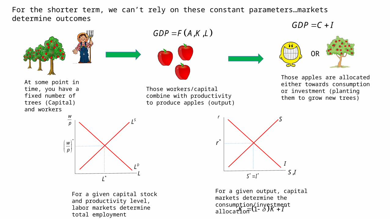
Recall, our story about the macro economy as an apple orchard…
At some point in time, you have a fixed number of trees (Capital) and workers
Those workers/capital combine with productivity to produce apples (output)
OR
Those apples are allocated either towards consumption or investment (planting them to grow new trees)
, ,GDP F A K L GDP C I
' 1
' 1 L
K K I
L g L
Investment today determines your capital stock next year. Population grows at a constant rate

At some point in time, you have a fixed number of trees (Capital) and workers
Those workers/capital combine with productivity to produce apples (output)
OR
Those apples are allocated either towards consumption or investment (planting them to grow new trees)
, ,GDP F A K LGDP C I
For the long term, we made some behavioral assumptions
PopPop
LF
LF
LL
Employment rate is constant (equal to one)
Participation rate is constant (equal to one)
1C Y I Y
Investment/Consumption rate is constant
At some point in time, you have a fixed number of trees (Capital) and workers
Those workers/capital combine with productivity to produce apples (output)
OR
Those apples are allocated either towards consumption or investment (planting them to grow new trees)
, ,GDP F A K LGDP C I
L
w
pSL
DL
*L
*w
p
For a given capital stock and productivity level, labor markets determine total employment
,S I
r S
I
* *S I
*r
For a given output, capital markets determine the consumption/investment allocation
For the shorter term, we can’t rely on these constant parameters…markets determine outcomes
' *1K K I

If you only learn one thing from microeconomics, it should be this…
Economic Decisions are Made at the Margin!!!!!
MB MCMarginal Benefit
Marginal Cost
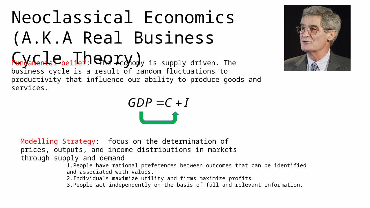
Neoclassical Economics (A.K.A Real Business Cycle Theory)Fundamental belief: The economy is supply driven. The business cycle is a result of random fluctuations to productivity that influence our ability to produce goods and services.
GDP C I
Modelling Strategy: focus on the determination of prices, outputs, and income distributions in markets through supply and demand
1.People have rational preferences between outcomes that can be identified and associated with values.2.Individuals maximize utility and firms maximize profits.3.People act independently on the basis of full and relevant information.
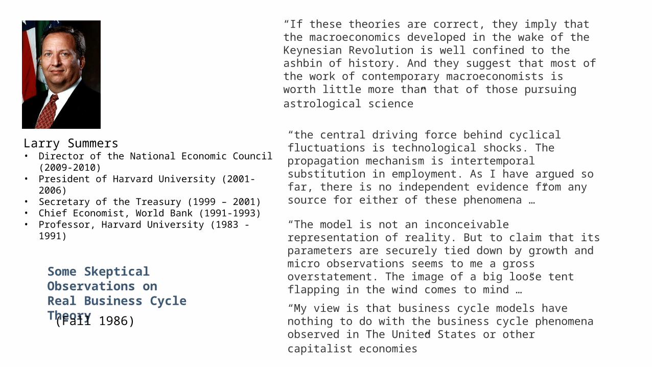
Larry Summers• Director of the National Economic Council (2009-2010)• President of Harvard University (2001-2006)• Secretary of the Treasury (1999 – 2001)• Chief Economist, World Bank (1991-1993)• Professor, Harvard University (1983 -1991)
“The model is not an inconceivable representation of reality. But to claim that its parameters are securely tied down by growth and micro observations seems to me a gross overstatement. The image of a big loose tent flapping in the wind comes to mind …”
“the central driving force behind cyclical fluctuations is technological shocks. The propagation mechanism is intertemporal substitution in employment. As I have argued so far, there is no independent evidence from any source for either of these phenomena …”
“If these theories are correct, they imply that the macroeconomics developed in the wake of the Keynesian Revolution is well confined to the ashbin of history. And they suggest that most of the work of contemporary macroeconomists is worth little more than that of those pursuing astrological science”
“My view is that business cycle models have nothing to do with the business cycle phenomena observed in The United States or other capitalist economies”
Some Skeptical Observations on Real Business Cycle Theory
(Fall 1986)
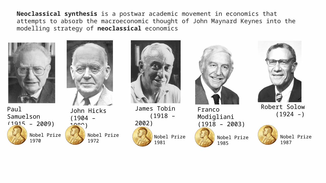
Neoclassical synthesis is a postwar academic movement in economics that attempts to absorb the macroeconomic thought of John Maynard Keynes into the modelling strategy of neoclassical economics
John Hicks (1904 – 1989)
Nobel Prize 1972
Paul Samuelson (1915 – 2009)
Nobel Prize 1970
Robert Solow (1924 –)
Nobel Prize 1987
James Tobin (1918 – 2002)
Nobel Prize 1981
Franco Modigliani (1918 – 2003)
Nobel Prize 1985