Final report - asset lives for State Water’s 2014 pricing proposal For the Australian Competition and Consumer Commission

9 December 2013

Liability limited by a scheme approved under Professional Standards Legislation. © 2013 Deloitte Access Economics Pty Ltd

Mr Darren Kearney Director Water Branch ACCC GPO Box 520 The Tower Melbourne Central MELBOURNE VIC 3000

9 December 2013

Dear Mr Kearney

Review of State Water Corporation’s proposed asset lives

We are pleased to submit our final report on our review of State Water’s asset life proposal.

Yours sincerely,

Paul Liggins Director Deloitte Access Economics Pty Ltd

Deloitte Access Economics Pty Ltd ACN: 149 633 116

Level 10, 550 Bourke St

Melbourne VIC 3000

GPO Box 78

MELBOURNE VIC 3001

Tel: +61 3 9671 7000

www.deloitte.com.au

Deloitte Access Economics Commercial-in-confidence

Contents 1 Background ..................................................................................................................... 1

1.1 Scope of work ................................................................................................................... 1

2 Analysis ........................................................................................................................... 2

2.1 State Water’s model ......................................................................................................... 2

2.2 A reasonable average remaining asset life for each valley.................................................. 6

2.3 The asset class breakdown for future capital expenditure ................................................. 9

2.4 Expected useful life for new assets .................................................................................. 11

Summary of conclusions.......................................................................................................... 14

Appendix A ............................................................................................................................. 16

Appendix B .............................................................................................................................. 19

Appendix C ............................................................................................................................. 21

Limitation of our work ............................................................................................................... 23

Analysis

1

1 Background

The Australian Competition and Consumer Commission (‘ACCC’) is currently reviewing charges for 2013-14 to 2016-17 proposed by State Water Corporation (‘State Water’). This review is being conducted pursuant to the Water Charge (Infrastructure) Rules 2010 (‘WCIR’).

State Water’s proposed charges are determined using a ‘building block’ cost build up, where charges reflect the sum of operating expenditure, a return on the value of assets, and depreciation.

As noted by the ACCC, asset lives are a key input in calculating the depreciation building block. They are the denominator for calculating the rate at which assets are depreciated. There are two types of asset lives generally used for depreciation purposes:

1. new capital expenditure will have standard asset lives applied in the year in which it occurs

2. existing assets, that are already partially depreciated, will have remaining asset lives applied to each asset category from the beginning of the regulatory period.

Appropriate lives are assigned to each asset class based on the asset type that make up the class and the useful economic lives expected from those assets.

1.1 Scope of work

Deloitte has been engaged by the ACCC to provide advice around the asset lives proposed by State Water. Specifically, the ACCC has asked us to consider and provide advice on: 1

1. Whether an average remaining asset life of 61.3 years for all existing assets as at 1 July 2014 is reasonable? Is it a reasonable average for each valley? If not, what is a more appropriate remaining asset life for each valley?

2. The asset class breakdown for future capex provided by State Water. Are these classes appropriate? Should there be additional asset classes?

3. For each of the asset classes determined in 2, provide an expected useful life for any new asset that would enter that class.

We have prepared this report based on our own research and analysis, discussions with the consulting engineers assisting Deloitte to review State Water’s opex and capex forecasts (Aurecon and Bird Consulting Group) and further discussions with State Water’s Manager Asset Services, Stephen Farrelley.

1 ACCC, State Water depreciation issues requiring further consultant advice, 8 August 2013.

Analysis

2

2 Analysis This section provides some background to the overall approach used by State Water to calculate asset lives, and then sets out our consideration of each of the three questions put to us by the ACCC.

2.1 State Water’s model

State Water uses a complex model to establish asset lives, including remaining asset lives. It is this model that calculates an average remaining life of 61.3 years for the existing asset base.

This model is fundamentally the same model that was examined by Atkins Cardno in 2009 as part of State Water’s pricing proposal to IPART.

State Water has described the methodology underlying the model, and in particular the average asset lives as follows:2

each asset’s (asset component’s) MEERA (modern engineering equivalent replacement asset) cost is established and expressed as a proportion of the entire asset portfolio (the weighted MEERA)

each asset’s effective life is calculated by taking the asset’s nominal life and adjusting it to reflect:

o Whether ‘parent’ assets have a shorter life than the asset in question

o The future asset service potential, including consideration of the current condition and proposed maintenance expenditure

o Whether the asset is to be run to failure or not

the average asset remaining life across State Water’s asset base is then the sum of each individual asset’s weighted MEERA value multiplied by the difference between its effective life and its current age

the average asset life is the sum of each individual asset’s weighted MEERA value multiplied by its effective life.

The future asset service potential plays an important role in determining the remaining asset life. All assets are allocated an overall condition score, which reflects a number of factors – including physical asset condition, legal limitations, service output and commercial considerations - which can range from 1 to 7. Each score then correlates to a percentage remaining life. Assets which have no future service potential (and hence no remaining life) are rated 1 and have 0-1% of their potential ‘as new’ life. Assets with substantial future service potential are rated 7 and have 98-100% of their potential ‘as new’ life. An asset rated 4 will have between 57% and 70% of its ‘as new’ life.

State Water’s processes for assessing future asset service potential is described in more detail in chapter 5 of its Total Asset Management Plan (TAMP).

2 State Water, Response to ACCC Information Request 2.4, 21 June 2013.

Analysis

3

The overall asset average asset life is to a large part determined by the asset lives allocated to a number of very large assets.

Atkins Cardno expressed a view that using a condition based asset life is appropriate and consistent with good practice, and that the current assumptions used around asset life were consistent with those used by other agencies in Australia. However Atkins Cardo queried or expressed concerns around:3

that ‘good and reliable data is available for only just over half the asset base’

there are difficulties in demonstrating a good calibration of the Weibull distribution for long life assets such as dams and structures

the ‘lumpiness’ of the relationship between the service potential schedule rating and remaining life

that the analysis does not apply two way adjustments to reflect the improvements in overall service potential from maintenance and enhancement expenditure.

Therefore, after assessing State Water’s model, Atkins Cardno concluded “Our opinion is that while there may well be a case to reduce the asset life from the current assumptions using condition based assessments, the analysis and data provided to us are not sufficiently robust to justify a change in the asset life assumptions applied to the 2006 determination.”4

We have not conducted a detailed re-review of the Atkins Cardno report or undertaken a detailed review of the methodology or integrity of the asset model. Indeed, the version of the model provided to us contains a number of #REF and #NAME errors caused by links to other models being broken or worksheets being removed prior to the model being provided to us. Thus our ability to examine the model was limited and the conclusions we have reached need to be viewed in this light.

Nevertheless, we can provide the following comments in relation to some of the matters raised by Atkins Cardno.

2.1.1 Good and reliable data

We agree that condition based assessments require good data on assets, and that asset information, particularly in respect of assets that have failed, should be updated regularly. Since the Atkins Cardno report updates to elements and individual assets within the model have occurred – for example as a result of the regular inspections of major dams. However, while State Water has advised that it intends to undertake 5-yearly wholesale updates of asset condition information, this has not occurred since 2009. Thus it is likely that many of the issues identified by Atkins Cardno regarding data are likely to remain.

We have recently completed a review of expenditure forecasts for 10 regional urban water businesses in Victoria. State Water is a much larger business, with typically longer life assets, than these regional urban businesses. We consider State Water’s asset data and

3 Atkins Cardno, Review of the Weighted Average Asset Life of State Water Corporation Asset, 11 December 2009, p. 4. 4 Atkins Cardno, Review of the Weighted Average Asset Life of State Water Corporation Asset, 11 December

2009, p. 17.

Analysis

4

systems are more robust than most of the regional water businesses we have reviewed, for reasons including:

because State Water’s assets are largely above-ground, information on asset condition is easier to obtain

asset condition assessments are used to inform replacement, not theoretical asset lives

regional Victorian water businesses’ risk assessment and prioritisation approach are generally less detailed in comparison to State Water’s approach

the regional Victorian water businesses which are using an asset condition assessment to inform asset management decisions are typically in the early days of doing so. State Water’s approach is relatively more mature.

2.1.2 Use of the Weibull distribution

The Weibull distribution function is widely used and accepted as a tool for forecasting asset failure, not only in the water industry but in other areas. It is appropriate for both long and short life assets. The difficulty in applying it to dams and similar structures is that obtaining data on failure or the point at which end-of life is reached is difficult – few, if any (in Australia) large dam structures fail or have reached their end of life in recent times. In fact in recent years the opposite has occurred as many dams have been upgraded or rehabilitated (for example, to comply with more stringent dam safety requirements) before end of life is reached. Thus, calibrating condition and failure rates becomes difficult.

This is not to suggest that the Weibull distribution should not be used for long-life assets such as dams, as other techniques for estimating remaining life will usually suffer from the same lack of data problem. Rather, it means that more caution needs to be used with interpreting outcomes for long life assets than other assets (where failure does occur on a more regular basis) as results are more uncertain. One way of exercising this caution, for example, is to undertake sensitivity analysis to examine the impact of alternative asset scores and outcomes. State Water’s model achieves this to some degree by using ‘upper ’, ‘midpoint’ and ‘lower’ remaining life percentages. Its proposed average remaining asset life of 61.3 years is based on the upper remaining life percentages. Average remaining lives are 47.2 and 53.4 years for the lower and midpoint life figures respectively.

2.1.3 Lumpiness of relationship between service potential score and remaining asset life

The relationship between service potential score and remaining asset life is somewhat ‘lumpy’. Atkins Cardno expressed concern about the steps between grades being different, implying that a more linear scale would be preferable.

While we note Atkins Cardno’s comments, there does not appear to be any clear justification or theoretical basis for a linear scale. It is more important that the scale reflect the relationship between score and remaining life. State Water’s advice is that the scale has been calibrated to empirically reflect this relationship, as outlined in the TAMP.

State Water has advised that linearising the scale would result in a significant reduction in the remaining useful life of its assets, although we have not tested this assertion.

Analysis

5

2.1.4 Two-way adjustments to reflect improvements in service potential

Following discussions with State Water, we do not agree with Atkins Cardno that the analysis does not enable two way adjustments to reflect improvements in service potential from maintenance and enhancement expenditure. We agree with State Water that the Atkins Cardno report is in error in this area and that where asset condition improves, for example as a result of expenditure, the condition score and hence asset life can be increased.5

2.1.5 Overall comments on State Water’s model for the purposes of determining remaining asset life

Having reviewed State Water’s asset model we agree with Atkins Cardno that it is not a perfect model for assessing remaining and total asset life, and that there are data limitations.

However, we consider that the limitations of the model are perhaps not as fatal as suggested by Atkins Cardno, and that:

as Atkins Cardno has indicated, the approach of using a condition based asset life is consistent with best practice

the use of the Weibull distribution is also consistent with best practice, and is generally appropriate for long life assets such as dams and structures, although it does rely on data being available

State Water’s approach to asset management and the determination of asset life is better than many other water businesses that we have reviewed in recent times.

On this basis we consider the overall asset life methodology proposed by State Water to be reasonable.6 Importantly, it is not clear to us that alternative approaches would produce a more accurate estimate of remaining asset lives.

5 In discussions with us State Water indicated that “the ‘Atkins review contains numerous errors of fact which we were not able to correct as we were provided no opportunity to comment or reply to their report”.

6 We note also that State Water’s Risk Based Asset Management Project won a Treasury Managed Fund award

for public sector innovation in enterprise risk management in 2010.

Analysis

6

2.2 A reasonable average remaining asset life for each valley

2.2.1 Is an average remaining life of 61.3 years at 1 July 2014 reasonable?

As noted, in order to assess whether an average remaining asset life of 61.3 years is reasonable we have examined State Water’s Asset life model. 7

This model includes water infrastructure assets across all of State Water’s valleys, with the exception of Lowbidgee.

The total value of assets in this model is $3.45 billion. Five assets account for one-fifth of the total being Blowering Dam structure ($120m), Burrendong Dam structure and concrete ($242m) Copeton Dam structure ($150m) and Glenbawn Dam structure ($141m).

It should be noted that the assets in the model do not include corporate (non-infrastructure) assets. We do not believe this will have a material impact on overall remaining asset life as:

our analysis suggests that doing so would have a very limited effect on average remaining asset life

State Water’s existing RAB does not include computers and motor vehicles, as the costs of these are reflected in internal charging which includes depreciation on the items.

In undertaking our calculations we have made a number of adjustments to the model as provided to us. By far the most material was to include only the assets related to the valleys that are subject to the ACCC’s review. The remaining asset life of 61.3 years advised by State Water includes all State Water’s regulated assets, including those in IPART-regulated valleys. The effect of including these IPART regulated valleys is to increase the overall remaining asset life. Key assets in the Murray Darling basin (MDB) are typically older than those in the IPART-regulated coastal valleys, which include a number of dams constructed in the 1970s and 1980s.8

The other adjustments we made were as follows:

excluded assets which are not assigned to a specific valley

excluded assets with negative remaining lives

excluded assets with zero values.

However, these three adjustments appear to make limited impact on the asset life calculations.

In determining the value-weighted average, we relied upon the ‘raw’ expected useful lives for asset lives outlined in State Water’s models, and so our estimate uses State Water’s

7 Email, 15 October 2013, State Water, 24 October 2013.

8 Including Toonumbar Dam (1971), Lostock Dam (1971), Glennies Creek Dam (1983) and Glenbawn Dam

(enlarged 1987).

Analysis

7

assumptions and methodologies for determining asset lives. We consider, however, that there was still sufficient information to make a reasonable estimate of remaining asset lives.

We have calculated a weighted average remaining life of State Water’s assets in the valleys under review of 50.91 years. This is less than the remaining life of 61.3 years proposed by State Water. As noted above, the main reason for this is the exclusion of the IPART- regulated assets.

2.2.2 Is 61.3 years an appropriate average remaining asset life for each valley? If not, what is a more appropriate remaining asset life for each valley?

Conceptually, remaining asset life is likely to differ across valleys. This is primarily because the major assets (dams) in each valley were constructed at different times. All other things being equal, more recently constructed assets (eg in the Peel valley) will have a longer asset life than assets constructed earlier (e.g. in the Macquarie valley). Having said this, the vast majority of major dams were constructed in a 20 year period from the late 1950s to the late 1970s, and hence the variation is not as great as it might otherwise be.

Table 1 – Year of construction of major dams

Dam Valley Year of construction

Pindari Dam Border 1969*

Oberon Dam Fish river / Macquarie 1959

Copeton Dam Gwydir 1973

Carcoar Dam Lachlan 1970

Wyangala Dam Lachlan 1935*

Burrendong Dam Macquarie 1967

Rydal Dam Macquarie 1957*

Hume Dam Murray 1936 (owned by MDBA)

Blowering Dam Murrumbidgee 1968

Burrinjuck Dam Murrumbidgee 1957

Keepit Dam Namoi 1960

Split Rock Dam Namoi 1987

Chaffey Dam Peel 1979 Source: Deloitte review of State Water’s website * Dams that have been enlarged since construction

We have used State Water’s models to estimate the average remaining lives for each valley. This was based on the same method outlined in section 2.2.1 but rather than calculating a total weighted average remaining life for all valleys, we have calculated the weighted average remaining life of each valley. This is set out in the table below:

Analysis

8

Table 2 – Average remaining life by valley

Valley Average remaining life

Border 53.88

Fish River 46.59

Macquarie 55.99

Gwydir 59.18

Lachlan 45.72

Murray 46.45

Murrumbidgee 40.88

Namoi 53.88

Peel 63.64

All ACCC regulated valleys 50.91

Hence the average remaining life of assets generally varies between 40 and 65 years across valleys, with an average (as discussed above) of approximately 50 years.

Key points to note are that:

there are no Lowbidgee assets in the models, hence we cannot estimate average asset lives for this valley

as noted above, these estimates are reliant on the assumptions and methodology used by State Water to estimate asset lives.

Given that the remaining asset lives differ by up to 50% from the valley to valley, and that prices are determined on a valley-by-valley basis, there is a prima facie case that different remaining asset lives should be used in different valleys. There are a number of ways these different remaining asset lives could be applied:

as point estimates based on the figures in table 2.

by rounding to the nearest 5 years – this results in the figures in table 3.

Table 3 – Average remaining life by valley

Valley Average remaining life

Murrumbidgee 40

Lachlan, Murray, Fish River 45

Border, Namoi, Macquarie 55

Gwydir 60

Peel 65

On balance, and given that there are some uncertainties and data issues with the model, using the rounded figures in the table 3 may be more appropriate than those in table 2. However, we also suggest that the ACCC undertake some modelling to examine the impact that the different asset lives have on price before it reaches a decision on the asset lives to

Analysis

9

be adopted. If the price impacts are minimal an argument for using common asset lives across valleys could be advanced on the grounds of administrative simplicity.

We note that State Water’s proposed average remaining asset life across all its regulated valleys of 61.3 years is similar to that adopted by Sydney Catchment Authority (SCA). SCA is probably the Australian water utility with the closest asset profile to that of State Water in terms of both the nature of its assets (predominately dams and transfer assets) and its overall asset age profile. SCA’s major storage, Warragamba dam, was completed in 1960 which makes it of similar vintage to several of SCA’s dams.

In its 2009 review of SCA’s prices IPART calculated regulatory depreciation using asset lives of 60 years for both new and existing assets. IPART also elected to use 60 years for new and existing assets in its 2012 decision on SCA’s prices.

2.3 The asset class breakdown for future capital expenditure

In State Water’s pricing application, it has proposed to categorise assets into ten classes:

Dams

Storage reservoirs

Revenue meters

IT systems

Plant & machinery

Office equipment

Buildings

Vehicles

Land

Work In Progress.

2.3.1 Are the asset classes for future capex reasonable? Should there be additional asset classes?

Regulators typically allocate assets into a number of broad asset classes with objectives including ensuring that:

the number of asset classes is manageable and that large and complex asset models are not required

the asset life for the respective class reflects the economic life of the assets in that category

decisions on how to allocate new assets into the various asset classes are straightforward

more complex assets do not need to be split up and allocated across classes. For example, the typical regulatory approach is to allocate a dam in its entirely to a single asset class rather than allocating the individual components (e.g. control tower, dam wall, gates, access road etc) to different asset classes.

Analysis

10

that assets with similar physical purposes and/or asset lives are placed in a the same set class.

To consider State Water’s approach it is first instructive to examine approaches used in other regulatory decisions.

We have reviewed asset classes used by other regulators for recent decisions in the water, and other industries. Our review included Unitywater, Queensland Urban Utilities, Allconnex Water (no longer operating from July 2012), SA Water, Western Water, Southern Rural Water, Central Highlands, Coliban Water, Gippsland Water, Barwon Water, APA GasNet and Powerlink.9

The number of asset classes proposed by State Water, 10, is in line with the number of classes used by other service providers (and accepted by other regulators)10

We then grouped identical or similar asset classes from these other service providers to help identify whether there were any asset classes that State Water should include or remove. For most asset classes proposed by State Water other than “Dams”, a number of other service providers use the same or similar asset classes. For example, three other service providers use “Land”, three use “Buildings” and two use “Vehicles”. Other asset classes had similar, although not identical matches. For example, rather than using “IT systems” as per State Water’s proposal, other service providers used classes such as “software”, “computer equipment” and “billing systems”.

We also examined the asset classes that other service providers used, which State Water did not propose. We found that there were a number of commonly used asset classes that were not proposed by State Water. These include classes for pipelines and miscellaneous assets. Some regulators also use sub-categories for separate classes of plant and equipment – for example electrical and/or mechanical equipment – although it is not clear that this breakup is necessary as generally the asset lives for both classes are similar and can be incorporated in a general ‘plant and equipment’ category.

In respect of pipelines, we understand that the Fish River Water supply scheme is the main area where Sate Water owns such assets. From this perspective it would be useful to have a separate asset category for pipelines, which tend to have an asset life that is shorter than dams or storage reservoirs but longer than the other asset categories. We have therefore included an estimate of the category “pipelines” in our analysis, although we do note that projected capital expenditure on pipelines is minimal.

In general we are satisfied that the number and type of asset classes proposed by State Water are generally a good match to the number and type of asset classes used by other service providers and regulators. In addition, they appear to appropriately reflect the nature of State Water’s asset base. For these reasons, we conclude that State Water’s

9 Given the three Queensland based service providers all used the same asset classes (albeit different asset lives), only one set of asset classes was used for this part of the analysis

10 The median includes State Water’s asset classes to determine where it lies relative to the number of asset classes used by other service providers. The average number does not include State Water (note that doing so would make the average closer to that of State Water’s number of asset classes).

Analysis

11

proposed asset classes are generally appropriate, although we suggest the inclusion of a pipeline category.

2.4 Expected useful life for new assets

State Water has proposed that all new capex be given a 102.4 year life. The ACCC has asked us, for each of the asset classes determined above, to provide an expected useful life for any new asset that would enter that class.

2.4.1 Analysis

The ACCC has advised that its general approach to depreciating assets is to ensure that the life assigned to each asset category accurately reflects the economic life of the asset types within that category.

As noted in section 2.3.1, we have grouped the asset classes proposed by State Water with identical and similar asset classes used by other service providers. Using these groupings, we have examined the asset lives used by other service providers for the asset classes proposed by State Water. This provided us with an estimated standard life for State Water’s asset classes. Given that it is common for regulators to match the asset life (for the purpose of depreciation) with the economic life of the asset, this type of analysis is relevant to our assessment.

We have also compared the resulting standard asset life estimates to the effective asset lives recommended by the Australian Tax Office (‘ATO’). The ATO seeks to set its (non-binding) asset life recommendations so that the recommended life matches the period over which a depreciable asset can produce income.11 The ATO asset lives are a valid comparator, as the ATO takes into account a range of matters into consideration when providing recommended asset lives in the water industry. This includes assets’ physical life as well as matters such as the physical life of the asset, manufacturer’s specifications, industry standards, retention periods, obsolescence, the past experience of asset users and scrapping or abandonment procedures.

2.4.2 Assessment

Grouping the similar asset classes of the different service providers allowed us to examine the asset lives used by other service providers and regulators for similar, or identical asset categories as those proposed by State Water.12

To arrive at our asset category life estimate, we have had strong regard to the median asset life used by the other service providers. We have also compared the median life used by other service providers with the effective lives of depreciating assets recommended by the ATO.

11 See http://law.ato.gov.au/pdf/pbr/tr2013-004.pdf and Income Tax Assessment Act 1997, section 40. 12

For this part of the analysis we used the asset lives reported by all three of the Queensland service providers mentioned in section 2.3.1. We did not, however, use the asset lives reported by Western Water because it used the same life for each category (similar to State Water’s current proposal), which is unlikely to reflect the actual lives of the underlying assets.

Analysis

12

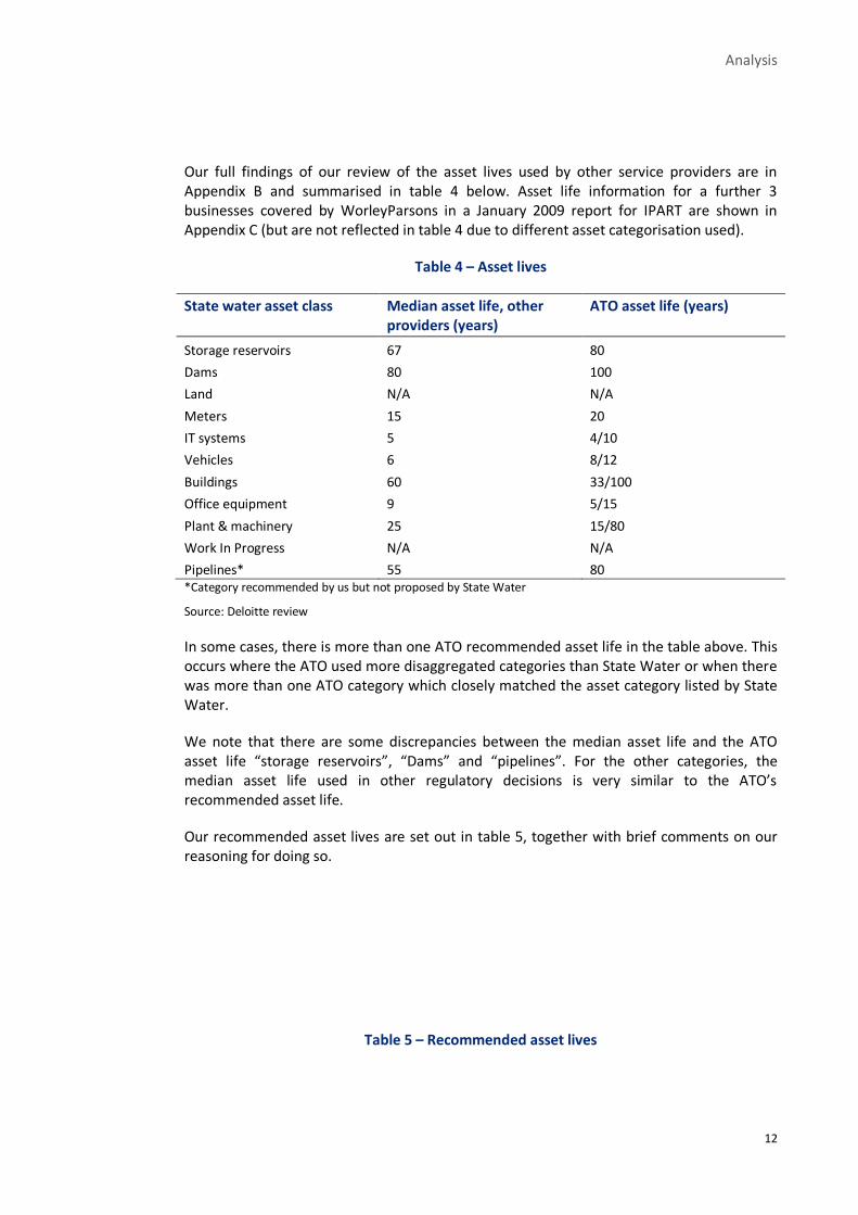
Our full findings of our review of the asset lives used by other service providers are in Appendix B and summarised in table 4 below. Asset life information for a further 3 businesses covered by WorleyParsons in a January 2009 report for IPART are shown in Appendix C (but are not reflected in table 4 due to different asset categorisation used).

Table 4 – Asset lives

State water asset class Median asset life, other providers (years)

ATO asset life (years)

Storage reservoirs 67 80

Dams 80 100

Land N/A N/A

Meters 15 20

IT systems 5 4/10

Vehicles 6 8/12

Buildings 60 33/100

Office equipment 9 5/15

Plant & machinery 25 15/80

Work In Progress N/A N/A

Pipelines* 55 80 *Category recommended by us but not proposed by State Water

Source: Deloitte review

In some cases, there is more than one ATO recommended asset life in the table above. This occurs where the ATO used more disaggregated categories than State Water or when there was more than one ATO category which closely matched the asset category listed by State Water.

We note that there are some discrepancies between the median asset life and the ATO asset life “storage reservoirs”, “Dams” and “pipelines”. For the other categories, the median asset life used in other regulatory decisions is very similar to the ATO’s recommended asset life.

Our recommended asset lives are set out in table 5, together with brief comments on our reasoning for doing so.

Table 5 – Recommended asset lives

Analysis

13

State Water asset class

Recommended asset life

Comment

Dams 100 Most water businesses and regulators use 100 years, although there are some exceptions where longer and shorter lives are used. Although it is possible for longer lives to be achieved, our view is that taking into account the long term possibility of asset stranding that 100 years is appropriate

Other Storages 80 Shorter life than dams. 80 years adopted by several key water utilities with bulk supply responsibilities

Land not depreciated

Meters 15 Commonly accepted asset life is 15 to 20 years. Given new irrigation meters have a relatively high level of new technology, we consider 15 years is appropriate.

IT systems 6 5 years is very common and generally accepted for software and hardware. At the same time, we note that specialised software and hardware typically has a longer asset life (say, 7-8 years), as it is often prudent to update and augment such items to prolong their life rather than incur the cost of new tailored solutions. We note that State Water has much expenditure in this category in the next regulatory period. On balance an average life of 6 years appears appropriate.

Vehicles 5 ATO recommendation is 8-12 years, however rural water authorities typically have heavier vehicle use than standard business use.

Buildings 60 Typical asset life adopted by many water utilities

Office equipment 10 Midpoint of the ATO range

Plant & machinery 25 Median of other utilities

Pipelines* 80 Future State Water pipelines are likely to be large diameter and relatively low pressure. Hence we suggest an asset life at the higher end of the range is appropriate

Analysis

14

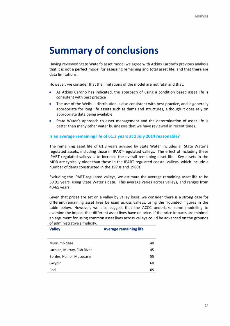
Summary of conclusions Having reviewed State Water’s asset model we agree with Atkins Cardno’s previous analysis that it is not a perfect model for assessing remaining and total asset life, and that there are data limitations.

However, we consider that the limitations of the model are not fatal and that:

As Atkins Cardno has indicated, the approach of using a condition based asset life is consistent with best practice

The use of the Weibull distribution is also consistent with best practice, and is generally appropriate for long life assets such as dams and structures, although it does rely on appropriate data being available

State Water’s approach to asset management and the determination of asset life is better than many other water businesses that we have reviewed in recent times.

Is an average remaining life of 61.3 years at 1 July 2014 reasonable?

The remaining asset life of 61.3 years advised by State Water includes all State Water’s regulated assets, including those in IPART-regulated valleys. The effect of including these IPART regulated valleys is to increase the overall remaining asset life. Key assets in the MDB are typically older than those in the IPART-regulated coastal valleys, which include a number of dams constructed in the 1970s and 1980s.

Excluding the IPART-regulated valleys, we estimate the average remaining asset life to be 50.91 years, using State Water’s data. This average varies across valleys, and ranges from 40-65 years.

Given that prices are set on a valley by valley basis, we consider there is a strong case for different remaining asset lives be used across valleys, using the ‘rounded’ figures in the table below. However, we also suggest that the ACCC undertake some modelling to examine the impact that different asset lives have on price. If the price impacts are minimal an argument for using common asset lives across valleys could be advanced on the grounds of administrative simplicity.

Valley Average remaining life

Murrumbidgee 40

Lachlan, Murray, Fish River 45

Border, Namoi, Macquarie 55

Gwydir 60

Peel 65

Analysis

15

Asset classes for future capex

In general we are satisfied that the number and type of asset classes proposed by State Water are generally a good match to the number and type of asset classes used by other service providers and regulators. In addition, they appear to appropriately reflect the nature of State Water’s asset base. For these reasons, we conclude that State Water’s proposed asset classes are generally appropriate, although we suggest the inclusion of a pipeline category.

Asset lives for future capex

Having regards to asset lives used by other regulators, water utilities and the ATO, and considering State Water’s circumstances, we recommend the following asset lives be used going forward:

State Water asset class Recommended asset life

Dams 100

Other Storages 80

Land not depreciated

Meters 15

IT systems 6

Vehicles 5

Buildings 60

Office equipment 10

Plant & machinery 25

Pipelines* 80

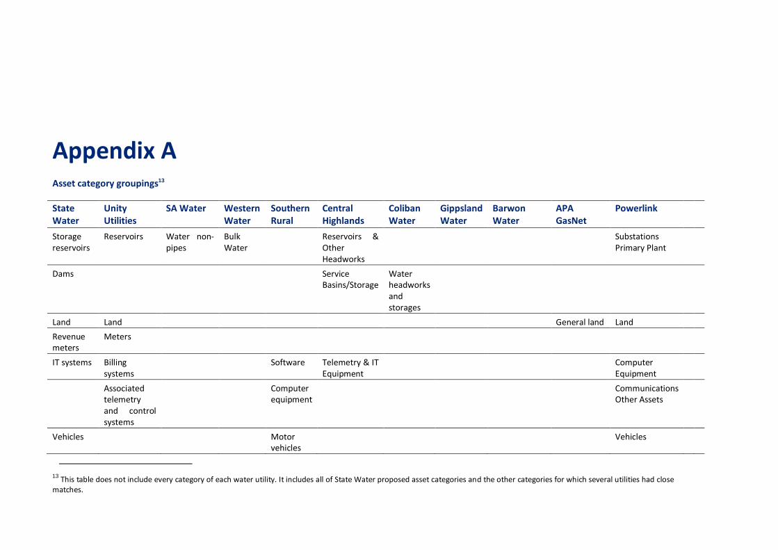
Appendix A Asset category groupings13

State Water

Unity Utilities

SA Water Western Water

Southern Rural

Central Highlands

Coliban Water

Gippsland Water

Barwon Water

APA GasNet

Powerlink

Storage reservoirs

Reservoirs Water non-pipes

Bulk Water

Reservoirs & Other Headworks

Substations Primary Plant

Dams Service Basins/Storage

Water headworks and storages

Land Land General land Land

Revenue meters

Meters

IT systems Billing systems

Software Telemetry & IT Equipment

Computer Equipment

Associated telemetry and control systems

Computer equipment

Communications Other Assets

Vehicles Motor vehicles

Vehicles

13 This table does not include every category of each water utility. It includes all of State Water proposed asset categories and the other categories for which several utilities had close matches.

17

Buildings Building other than infrastructure housing

Buildings General buildings

Commercial Buildings

Office equipment

Corporate systems

Sewer corporate depreciation

Corporate Office Furniture & Miscellaneous

Support services

Water corporate depreciable

Office Machines

Plant & machinery

Pump stations

Adelaide Desalination Plant

Recycled Water

Plant & Equipment

Compressors Moveable Plant

Substations Secondary Systems

Network Switching Centres

Work In Progress

Water corporate non depreciable

sewer corporate non depreciable

18

Mains Water pipes Water Pipeline repair

Wastewater - Sewers & Mains

Sewer pipelines and pump stations

Water Pipelines & Networks

Water Mains Replacements

Pipelines Transmission Lines - Overhead

Sewer Pipes Sewerage Mains, Water Fittings Etc

Water pipelines and network

Melbourne to Geelong pipeline

Transmission Lines - Underground

Mains, Water Fittings Etc

Transmission Lines - Refit

Treatment Water treatment

Water Treatment

Odourant plants

Sewerage treatment

Waste Treatment

Gas quality

Sundry property, plant and equipment

Other tools and equipment

Other

19

Appendix B

State14 Water asset class

Unity Water

QUU

Allconex water

SA Water

Southern Rural Water

Central Highlands

Coliban Water

Gippsland Water

Barwon Water

APA GasNet

Powerlink Median

Storage reservoirs

54 90 70 64 40 67.0

Dams 99 60 79.5

Land NA NA NA NA NA NA NA NA

Revenue meters 35 15 15 15.0

IT systems* 5,22 5,10 5,20 5,7 5 5,15 5

Vehicles 5 7 5.8

Buildings 60 60 60 66 60 40 60.0

Office equipment*

13 10 5 15 10 7

5 5 15 7 8.5

Plant & machinery*

34 25 25 57 11 30 7, 12, 15 25

Pipelines** 55 70 70 103 30 55 50, 60 60 67,100 55 30,45, 50 55

14 Table does not include Western Water because the asset lives it used for each category was the same—66.67 years.

20

*Denotes State Water’s asset categories for which other service providers have more than one similar category, meaning asset life estimates are based on the median of all the like categories of other service providers.

**Not an asset class proposed by State Water, but proposed by Deloitte.

21

Appendix C – WorleyParsons 2009 review of asset lives for Sydney Catchment Authority – reported lives for various water utilities

Asset category class SCA Melbourne Water ActewAGL WA Watercorp

Dams 200/100 100 200 100

Treatment Plants

45 80/25 50/60 80/50/25/20

Pipelines 120/100 80 80 80

Tunnels

100 80 80 80

Reservoirs/tanks 150 80 80 80

Pump stations 45 80/25/10 35 to 60 100/40/25/20

Mechanical Equipment 100/50 25 25

Electrical Equipment 40 25 20/40

SCADA Equipment 40 10 10

Office equipment 5 15/10/5

Computer equipment 5 3 4

22

Furniture 10 10/15/10

Office amenities 10 15/10/5

Operation Equipment 6 7/5/3

Buildings 30/50 40 33.3/100

Fencing/Landscaping 20 40 20

Unsurfaced Roads 100 20/30/40/50

Bridges 100 40 20/50

Vehicles 7 8

Systems/software 5 3

Land Perpetuity Perpetuity Perpetuity

Limitation of our work

General use restriction

This report is prepared solely for the internal use of the Australian Competition and Consumer Commission. This report is not intended to and should not be used or relied upon by anyone else and we accept no duty of care to any other person or entity. The report has been prepared for the purpose described in section 1.1. You should not refer to or use our name or the advice for any other purpose

Contact us

Deloitte Access Economics ACN: 149 633 116 Level 10 550 Bourke Street Melbourne VIC 3000 GPO Box 78 Melbourne VIC 3001 Australia Tel: ++61 3 9671 7000 www.deloitteaccesseconomics.com.au

Deloitte Access Economics is Australia’s pre-eminent economics advisory practice and a member of Deloitte's global economics group. The Directors and staff of Access Economics joined Deloitte in early 2011.

About Deloitte

Deloitte refers to one or more of Deloitte Touche Tohmatsu Limited, a UK private company limited by guarantee, and its network of member firms, each of which is a legally separate and independent entity. Please see www.deloitte.com/au/about for a detailed description of the legal structure of Deloitte Touche Tohmatsu Limited and its member firms.

Deloitte provides audit, tax, consulting, and financial advisory services to public and private clients spanning multiple industries. With a globally connected network of member firms in more than 150 countries, Deloitte brings world-class capabilities and deep local expertise to help clients succeed wherever they operate. Deloitte's approximately 200,000 professionals are committed to becoming the standard of excellence.

About Deloitte Australia

In Australia, the member firm is the Australian partnership of Deloitte Touche Tohmatsu. As one of Australia’s leading professional services firms. Deloitte Touche Tohmatsu and its affiliates provide audit, tax, consulting, and financial advisory services through approximately 6,000 people across the country. Focused on the creation of value and growth, and known as an employer of choice for innovative human resources programs, we are dedicated to helping our clients and our people excel. For more information, please visit our web site at www.deloitte.com.au.

Liability limited by a scheme approved under Professional Standards Legislation.

Member of Deloitte Touche Tohmatsu Limited

© 2013 Deloitte Access Economics Pty Ltd