Universite Laval

Food vulnerability in Guatemala: a staticgeneral equilibrium analysis

Renato VargasPamela EscobarMaynor Cabrera

Javier CabreraVioleta Hernández

Vivian Guzmán

July 2016

Final report

Food vulnerability in Guatemala: a static general equilibrium analysis

Abstract

In this study, we used a Computable General Equilibrium model of the Guatemalan economy toconduct simulations for a) a reduction in productivity due to climate change; and b) the effects ofdrought in agriculture. The reduction in productivity due to climate change would mean an importantdrop in the value added of agriculture and animal production, as well as a slight drop in industrial foodproduction and the service industry. Under this scenario we could expect a fall in real GDP of 1.2%. Thereduction of productivity could mean a reduced fiscal space, and a reduction in governmentexpenditure because of lower tax revenues. More importantly, due to higher prices and lower incomeof households, this scenario could mean that consumption of agricultural goods for each type ofhousehold would be reduced in a relevant manner with great impacts to the food security aspect ofaccess. One of the findings in the effects of drought in agriculture is a decrease of the value added in23%. As expected, this situation negatively affected the wages paid to unskilled workers, but also urbannon-poor households would saw a reduction of their disposable income due to higher food prices.One of the most interesting results is that the demand for land would fall down by 38 per cent. This isbecause as water would become scarcer, there would be fewer incentives to engage in agriculturalactivities. However, due to the importance of agricultural production for ensuring food security, thisresults show that a proper water allocation system is needed.

JEL: R15, R22, Q12.

Keywords: Regional Economics Measurement, Computable General Equilibrium, SpatialAnalysis, Natural Resource, Agricultural Employment, Farm Household, Farm Input Markets,

Authors

Renato Vargas:Economist, independentGuatemala City, Guatemalarenovargas [at] gmail [dot] com

Pamela Escobar:Systems Engineer, independentGuatemala City, Guatemalapescobarf [at] gmail [dot] com

Maynor Cabrera:Economist, Fedes.orgGuatemala City, Guatemalamaynor.cabrera [at] fedes [dot] org

Javier Cabrera:Economics undergraduate studentGuatemala City, Guatemalajacava.84 [at] gmail [dot] com

Violeta Hernández:Economist, independentGuatemala City, Guatemalavioletaehernandezc [at] gmail [dot] com

Vivian Guzmán:Economist, independentGuatemala City, Guatemalavvguzman [at] gmail [dot] com

Acknowledgements

This research work was carried out with financial and scientific support from the Partnership forEconomic Policy (PEP) (www.pep-net.org) with funding from the Department for InternationalDevelopment (DFID) of the United Kingdom (or UK Aid), and the Government of Canada through theInternational Development Research Center (IDRC). The authors are also grateful to Martin Cicowiezfor technical support and guidance, as well as the peer reviewers for their valuable comments andsuggestions.

Contents

1 Introduction ...................................................................................................................................... 7

1.1 Context of the study ................................................................................................................ 7

1.2 Research questions and objectives .......................................................................................... 8

2 Literature review .............................................................................................................................. 8

2.1 CGE models for food security analysis................................................................................... 8

2.2 Regarding food security and agriculture ................................................................................. 9

2.3 Food security under climate change and more dependence on technology .......................... 10

3 Model and data ............................................................................................................................... 11

3.1 Model .................................................................................................................................... 12

3.2 Data ....................................................................................................................................... 12

3.3 Guatemala’s economic structure ........................................................................................... 14

4 Application and results ................................................................................................................... 18

4.1 Results from simulations....................................................................................................... 18

5 Lessons learned, innovations and policy implications ................................................................... 22

6 References ...................................................................................................................................... 23

7 Annex ............................................................................................................................................. 27

7.1 Constructing of the Social Accounting Matrix for Guatemala ............................................. 27

7.2 Guatemala's economic structure tables ................................................................................. 35

7.3 Sensitivity results .................................................................................................................. 36

List of tables

Table 1 - Technologies that would have the largest global effect on a price reduction and yield increasein 2050, by crop...................................................................................................................................... 11

Table 2 - Macro SAM (in millions of Quetzales)................................................................................... 13

Table 3 - Added value per sector (millions of Quetzales and percentage) ............................................. 14

Table 4 - Exports and imports by commodity (in percentage) ............................................................... 15

Table 5 - Factorial composition of value added (percentage) ................................................................ 16

Table 6 - Distribution of income for each household group (percentage).............................................. 16

Table 7 - Income composition for each household group (Percentage) ................................................. 17

Table 8 - GDP table (% change)............................................................................................................. 19

Table 9 - Agricultural goods: Price and consumption by household type (% change) .......................... 19

Table 10 - GDP table (% change)........................................................................................................... 20

Table 11 - Exports and imports by product (% change)......................................................................... 21

Table 12 - Macro SAM........................................................................................................................... 27

Table 13 – Commodity and Economic Activity Aggregation for the Micro SAM ................................ 29

Table 14 - Participation in activities income by skill level (percentage)................................................ 30

Table 15 - Activities of the SAM according to the activities included in the survey............................. 31

Table 16 - Share of each group of household (percentage) .................................................................... 31

Table 17 - Share of income for each household group........................................................................... 32

Table 18 - Household expenditure in good and services according to household groups (percentage). 33

Table 19 - Consumption composition of each household group (percentage) ....................................... 35

List of figures

Figure 1 - Aggregate output by industry in scenario of decrease of TFP (% change)............................ 19

Figure 2 - Water use by industry (% total) ............................................................................................. 20

Figure 3 - Change in value added by sector, by simulation scenario ..................................................... 21

Figure 4 - Sensitivity results................................................................................................................... 36

List of acronyms

AIS Secure Agricultural Income ProgramBANGUAT Central Bank of GuatemalaFAO Food and Agriculture Organization of the United NationsGDP Gross domestic productGDPFC Gross Domestic Product at Factor CostGDPMP Gross Domestic Product at Market PricesGTAP Global Trade Analysis ProjectIAHS International Association of Hydrological SciencesIFPRI International Food Policy Research InstituteINAB National Forestry Institute of GuatemalaINE National Institute of Statistics of GuatemalaLSMS Living Standards Measurement SurveyMACEPES Model of Exogenous Shocks and Economic and Social ProtectionMAGA Ministry of Agriculture, Livestock and Food of GuatemalaMams Maquette for simulation of the Millennium Development GoalsMDG Millennium Development GoalsNDP National Development Plan of GuatemalaNetIndTaxPEP 1-1 model Partnership for Economic Policy Standard Computable General

Equilibrium Model Single-Country, Static VersionPFN National Forestry Program of GuatemalaPROBOSQUE Programme for promoting the establishment, recovery, restoration,

management, production and protection of forests in GuatemalaSAM Social Accounting MatrixSEEA System of Environmental and Economic AccountsSEGEPLAN Secretariat for Planning of the Presidency of GuatemalaSUT Supply and Use TablesTFP Total factor productivityUNESCO IHP International Hydrological Programme of the United Nations

Educational, Scientific and Cultural OrganizationWMO World Meteorological Organization

1 Introduction

1.1 Context of the study

Food security is an important issue in Guatemala, not only because of availability, but also because ofdifficulties of access from households. For example, maize and beans, the staple crops behind theGuatemalan diet are characterized by low agricultural yields and absolutely no use of artificial irrigation(INE, 2011). There is certainly a lack of technology among the small-scale farmers, but one of the greaterconcerns lately is the variability of climate and its impact on the risk of producers. Moreover, there is ahigh dependence of some agricultural goods on imports, and consequently the country has becomevulnerable to the rise of international food prices. Guatemala is considered a low food-secure country(Yu, You, & Fan, 2010).

The agricultural sector is key to food security and it is important to understand the linkages between theeconomy and its various components in a systemic manner. Agricultural and food security aspects of theSystem of Environmental and Economic Accounts of Guatemala (SEEA) have shown key insights intothese linkages. For example, it is interesting to notice that maize–the staple crop–production inGuatemala depends entirely on rain water for its growth (INE, 2011). This exposes the production of thiscrop to considerable risk in terms of climate variability, which contrasts with the fact that after sugarcane and bananas, maize is one of the main products of the country in terms of volume.

A similar argument can be made of beans, which also depend entirely on rain water (INE, 2011). Beanscover a relevant portion of the Guatemalan diet, and it is interesting to see how the canned variety areincreasingly used by households. This form of consumption of beans is ever more present in urbankitchens and it might represent a cultural shift that might increase the importance of industrial foodprocessing in the food chain.

We must recognize the share of agricultural output used by manufacturing industries at the national level.For example, in the case of maize, only 20% of all used volume had a final destination in manufacturing.This is consistent with the 80% (adjusted to extract the negative stock variation) that was consumed byhouseholds. It contrasts with the 99% of the supply of unprocessed rice and wheat that were used almostexclusively by the food processing industries (INE, 2011). This does not mean that households did notconsume such products. It only means that they got them in their processed versions, such as precookedwhite rice and dehydrated breakfast gruel. For this very reason, the totality of sugar cane was used bythe food processing industry (INE, 2011).

Aside from these exceptions, households did consume large volumes of cultivated products directly,which is consistent with the traditional market culture still present in most of the country. For example,they used 95% of beans, 88% of potatoes, 97% of other roots and tubers, 99% of fresh culinary herbs,91% of other vegetables and 67% of all fruits, among others (INE, 2011).

According to the Living Standards Measurement Survey –LSMS 2011, in 2011, 33.5% of the employedpopulation of 15 years old and over from Guatemala, was employed in the agricultural sector (43.6% ofmen and 16.1% of women). Of the total employed in agriculture, 78.5% lived in rural areas and 71.3%was below the poverty line. In addition, more than a third of those employed in this sector (37.1%) wereof ages between 15 and 24, and 7 out of 10, and had incomplete primary education or less. For that sameyear, only 6.8% of those employed in agriculture were formally employed (at a national level, over 30%of the employed population were working in the formal sector).

In the case of natural resources, water faces several stresses in terms of quantity and quality. Thesepressures are related to human interventions like agriculture and land use change. According to Llop &Ponce (2012), CGE and water analysis at national scale had studied a broad type of issues like water

pricing policy, water allocation, water markets and climate change impacts. Under different approachesand scope of analysis, any shock in water availability would have great implications on agriculturalproduction and on inequality as we will see in the results section. These facts frame our simulationsappropriately and they allow us to provide an intuition for the observed changes.

1.2 Research questions and objectives

Because rural population has serious social disadvantages in terms of poverty and access to food, one onthe main challenges of the economic policy is the creation of jobs in rural areas that will allow familiesto afford sufficient nutrition. With a long history of strong reliance of the Guatemalan economy in theagricultural sector and lack of creation of quality jobs, the policy questions are:

What are the impacts of climate variability on food security, growth and employment? What can we expect from the share of contribution to GDP of the Agricultural industry given

this variability? Will climate variability have an effect on water use according to the current base line?

2 Literature review

2.1 CGE models for food security analysis

We understand food security as convened at the World Summit on Food Security (2009): “Food securityexists when all people, at all times, have physical, social and economic access to sufficient, safe, andnutritious food to meet their dietary needs and food preferences for an active and healthy life. The fourpillars of food security are availability, access, utili[z]ation and stability. The nutritional dimension isintegral to the concept of food security.”

According to a comprehensive report conducted in Guatemala by IARNA-URL, IICA, & McGillUniversity (2015), food security issues are essentially multidimensional problem, where variouselements carrying different impacts on food availability, access, and the ability to utilize and benefitfrom food. In that regard, computable general equilibrium models allow for the simultaneous evaluationof various aspects of the food security problem, such as food prices, income and expenditure, as well aseconomy-wide implications of food policies.

In a review, Saravia-Matus, Gomez, & Mary (2012) explain that the main economic problems regardingfood security seem to be the under-nourishment of people in rural areas of low-income countries, due tolack of access to food, resources, and technology, on the one hand, and the volatility of food markets thatthreatens high-income countries, on the other. They explain that the scientific literature that addressesthese problems from an economic perspective can be divided into studies that deal with increasingagricultural productivity by various means; those that discuss the macroeconomic analysis of pricevolatility, trade and market stability; and a cluster of studies that deal with the effects of demand forbiofuels, farmland acquisition, and the food price crisis on small-scale farmers.

Food availability, thus, is only one piece of the puzzle. In the seminal work of Sen (1998) and follow upstudies (Tomlinson 2011; and Smith et al., 2000), it is clear that the ability of people to buy food is themost relevant factor regarding the lack of food security, even in countries where food availability is notan issue.

Besides, any shock in water availability will have great implications for agricultural production and forfood security, specially for countries like Guatemala where production of some crops are heavily

dependent on rainfall and water resources are facing several stresses in terms of quantity and quality.These pressures are related to human interventions like agriculture and land use change (Ponce et al.,2012). According to Ponce et al., (2012) CGE and water analysis at national scale had studied a broadtype of issues like water pricing policy, water allocation, water markets and climate change impacts.Under different approach and scope of analysis, any shock in water availability will have greatimplications for agricultural production and for food security.

Despite food security is a big concern for Guatemala, local researchers have not used CGE models toanalyze this situation. Most of the applications of CGE models for Guatemala have been few. Vasquez(2008) applied an integrated macro-micro model to analyze Millennium Development Goals -MDG1 andCabrera, et. Al (2010) implemented the Model of Exogenous Shocks and Economic and SocialProtection - MACEPES-2 to analyze impact of external shocks in poverty and inequality3.

2.2 Regarding food security and agriculture

Low and middle-income countries have been under the spotlight due to the prevalence of food insecurity.As a result, there has been a global effort to reduce malnourishment as expressed by the MDG that wereset to be achieved in 2015. By the end of that year, the United Nations Organization acknowledged that“the proportion of undernourished people in the developing regions has fallen by almost half since 1990,from 23.3 per cent in 1990–1992 to 12.9 per cent in 2014–2016” (United Nations, 2015).

However, the results differ widely by region and country. For instance, Latin America is one of theregions that reached the target of halving the proportion of people who suffer from hunger. Among theregion, Nicaragua and Peru showed the greatest improvement, while Guatemala was the only country toshow no progress on eradicating hunger (FAO, 2015). By 2015, Guatemala still had 15.6 per cent of itspopulation living below minimum dietary levels (in 1991, this rate was 14.9 per cent according to theUnited Nations, 2016). Therefore, efforts to reduce hunger continue to be important.

There are several factors that are making Guatemala fall behind globally. For example, maize and beans,the staple crops behind the Guatemalan diet have shown low agricultural yields and absolutely no use ofartificial irrigation (INE, 2011), influenced not only by the lack of technology among the small-scalefarmers, but also because of adverse climate conditions4. At the same time, the country depends on theimport of agricultural goods5 which means that the country has recently experienced rising food importprices and exports that cannot keep up. For those reasons, Yu, You, & Fan (2010) consider it to be a lowfood-secure country.

More recently, it has been argued that the most food-insecure countries “frequently have higher politicalstability risk and corruption levels, alongside weaker institutions that fail to provide appropriategovernment regulation and oversight” (Economist Intelligence Unit, 2014). Guatemala is one of the

1 The macro-micro model called MAMS (Maquette for simulation of the Millennium Development Goals -MDG-, described indetail in Lofgren et al., 2013). This study was developed under the Project “Políticas públicas para el desarrollo humano: ¿Cómolograr los objetivos de desarrollo del milenio en América latina y el Caribe?” of UNDP, UN/DESA, The World Bank andUN/ECLAC, developed in 18 countries in Latin America.2 Thi study was developed under the Project “Implicaciones de la Política Macroeconómica, los Choques Externos, y losSistemas de Protección Social en la Pobreza, la Desigualdad y la Vulnerabilidad en América Latina y el Caribe”, coordinatedby ECLAC and UN/DESA.3 Using a Macro-Micro approach, see Vos et al. (2010).4 Guatemala occupies the tenth position in the Global Climate Risk Index 2016, which means that it is one of the countries thathas suffered the most from extreme weather events between 1995 and 2014 (Kreft, Eckstein, Dorsch, & Fischer, 2015).5 In 2010, the supply of wheat, rice and maize came from import flows (99.7%, 69.5% and 21.3% of total offer, respectively).

countries that falls into this description and this may undermine the capabilities to reach its food policies’objectives.

2.3 Food security under climate change and more dependence ontechnology

Conforti (2011) identifies some of main long term drivers of change in food systems that are relevant forthe analysis of the Guatemalan case:

The demand of agricultural products will grow steadily: according to Alexandratos & Bruinsma(2012), the global demand for agricultural products is expected to grow at an annual rate of 1.1 per centbetween 2005 and 2050. This growth is influenced by the increase of the global population,improvements of per capita income, and diet changes that include more livestock products. Altogether,these factors are expected to create pressure on natural resources, and according to the IFPRI IMPACTmodel, prices for maize, rice, and wheat would increase by 104, 79, and 88 per cent, respectively by2050 (Rosegrant, et al., 2014).

A price increase on these vital products will impact countries like Guatemala, as the import shares ofthese products are high. In fact, from past events, Torero & Robles (2010) have estimated that a 10 percent rise in food prices would increase the national poverty rate in 0.9 percentual points, affecting mainlyurban households.

Climate change is expected to influence food security:

Scientists have largely explored the impact that climate change has on agriculture because “water-relatedhazards account for 90% of all natural hazards and their frequency and intensity is generally rising”(UNESCO, 2013). This means that spatial and temporal patterns of precipitation and water availabilityhave been changing, and it implies more dry spells, droughts or floods across the world. Either of theseevents could have the following effects:

Economic effects: the increasingly erratic rainfall and high temperatures, among other factors,can significantly reduce food availability in low-latitude countries (Porter, et al., 2014). In fact,Cline (2007) expects that agricultural productivity in Latin America will decrease between 13 to24 per cent by the 2080s. Therefore, this implies, at a local level, that poor households thatusually depend on agriculture would be more prone to lose a larger fraction of their assets andincome. At a national level, countries in this region would progressively need to import foodfrom other markets to meet their demand.

In specific for Guatemala, under certain climate conditions forecasted by the IntergovernmentalPanel on Climate Change, in 2030, the maize yields could vary between -6.7 and -3.8 per cent,those of the bean could vary from -6.9 to 1.5 per cent, and the rice yields could vary between -10.4 and -7.5 per cent (Comisión Económica para América Latina y El Caribe, 2013).

Aditionally, Antle & Capalbo (2010) urge everyone to look beyond agriculture. They mentionthat the economic impact of climate change will not only affect agriculture but other economicactivities as well. However, these potential impacts remain higly unexplored. They list potentialissues related to “the effects of sea level rise on transportation infrastructure, changes in thedesign and location of storage facilities, …, the effects of regulatory policies on adaptive capacityof the food system”, among others. As a result, strategies to cope with climate change shouldhave a broader scope.

Biological effects: according to FAO (2008) and Tirado et al. (2010), some foodborne andwaterborne pathogens and diseases (like cholera, mycotoxins and phycotoxins) are related toextreme weather events. This means that the variation of humidity, precipitation and temperaturecan have a real effect on food safety and human health. In specific, Hallegatte et al. (2016) havehighlighted that poor people and children are more likely to suffer diseases related to theinfluence of climate change on food quality.

Governance effects: UNESCO-IHP, WMO & IAHS (2016) highlight that water governance isone of the main concerns for economic growth and development. As water scarcity will continue,competition for water use will rise and countries need to build a platform for the discussion andresolution of water-related conflicts (water rights, privatization, water pricing, etcetera).Otherwise, these conflicts will frustrate the efforts towards poverty reduction and food security.

In short, the impact of climate change on agriculture has been largely explored, and it can be seen thatthe effects range from economic to biological and governance issues. Altogether, it is clear that a country-level assessment on climate change issues should be done in order to set mitigation and adaptationmeasures.

The adoption of technology will be key for agricultural productivity: at a global level, there is enoughfood for everyone to be nourished (World Food Programme, 2011), as a result of technological progress.In the following years, the agricultural activity is expected to become more dependent on technologyadoption due to the challenges derived from climate change (IFPRI, 2016).

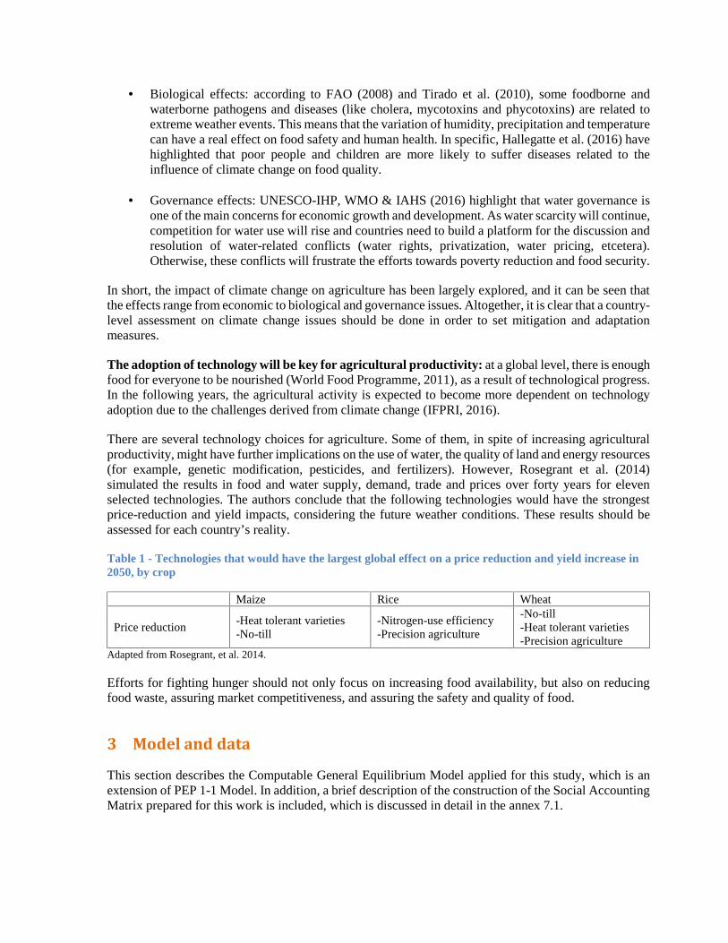
There are several technology choices for agriculture. Some of them, in spite of increasing agriculturalproductivity, might have further implications on the use of water, the quality of land and energy resources(for example, genetic modification, pesticides, and fertilizers). However, Rosegrant et al. (2014)simulated the results in food and water supply, demand, trade and prices over forty years for elevenselected technologies. The authors conclude that the following technologies would have the strongestprice-reduction and yield impacts, considering the future weather conditions. These results should beassessed for each country’s reality.

Table 1 - Technologies that would have the largest global effect on a price reduction and yield increase in2050, by crop

Maize Rice Wheat

Price reduction-Heat tolerant varieties-No-till

-Nitrogen-use efficiency-Precision agriculture

-No-till-Heat tolerant varieties-Precision agriculture

Adapted from Rosegrant, et al. 2014.

Efforts for fighting hunger should not only focus on increasing food availability, but also on reducingfood waste, assuring market competitiveness, and assuring the safety and quality of food.

3 Model and data

This section describes the Computable General Equilibrium Model applied for this study, which is anextension of PEP 1-1 Model. In addition, a brief description of the construction of the Social AccountingMatrix prepared for this work is included, which is discussed in detail in the annex 7.1.

3.1 Model

In this study, we apply an extended version of the PEP 1-1 Model by Decaluwé et al. (2013) withextensions for the inclusion of water, based on Banerjee, Cicowiez, Horridge, and Vargas (2016) andmodifications as explained hereafter6.

The closure specification includes an option to specify mobile capital or sector specific; with the clearingvariable in the government closure with endogenous government savings, endogenous governmentconsumption, endogenous direct tax on households or endogenous indirect tax on commodities.

The closure of rest of the world could be by real exchange rate adjustment or foreign savings; and thesavings-investment closure could be using fixed or flexible investment. To take into consideration thedifferent remunerations of labor by economic activity, this extension includes the numbers of workers,which allows us to calculate a factor of wage differences across all industries.

The model is able to handle several shocks like increase in labor supply, changes in world price of exportsand imports, change in capital stock, changes in government consumption, decrease in taxes, subsidieson capital, decrease in margins and changes in total factor productivity. Finally, the model features anextension to include water as an economic factor with price zero if supply is greater than demand, but inthe opposite scenario, the model estimates a price for this scarce natural resource, simulating theexistence of market of water or internalizing the cost of provide water to economic activities.

For the demand for exports, we assume that Guatemala is a small country or price taker in internationalmarkets, and in the external sector closure we suppose that we have limits to international finance. Theadjustment in this sense has to be done via real exchange rate. We also assumed that capital is mobile.Government will adjust its consumption to maintain a level of savings,7 to incorporate costs of fiscalrevenues reduction, in a scenario where it is very difficult to pass a tax reform. Finally, we assumed thatreal investment was fixed and savings had to be adjusted to maintain the same level of real gross fixedcapital formation.

Income elasticities of demand were estimated using micro-data of LSMS 2011. We use elasticities ofproduction close to those provided by the model and for value added we use those for GTAP (Narayan,Badri, Aguiar & McDougall, 2012).8 Finally, for Armington and CET elasticities we use estimations forsimilar economies to Guatemala, like Ecuador, Mexico and Filipinas, that were compiled by Annabi,Cockburn & Decaluwé (2006).

3.2 Data

First, we compiled a Macro SAM, rearranging information from SAM 2011 into an aggregated formatderived from an analytical perspective of the System of Environmental and Economic Accounts forAgriculture, Forestry, and Fisheries, which has a strong emphasis on food security issues. Second, wedisaggregated the labor factor using information from the Household Survey. Next, we used data fromGTAP to split the capital factor between capital and land. Since it was necessary to have a specificremuneration for the land factor, we used the relative structure from GTAP. Fourth, we rearranged the

6 Extensions were conducted with the help of Martin Cicowiez.7 Although our chosen assumption better reflects the reality of Guatemala, we are aware that it's difficult to conduct a welfareanalysis, given that government consumption is not a determinant of household utitlity. For welfare analysis, a closure withfixed government consumption and real savings would be preferable, using direct taxes to clear the government budget.8 These elasticities are relatively lower for resource sectors and higher for manufacturing and services sectors.

SUT information in order to disaggregate activities in SAM. Fifth, using household survey estimates weopened household information. Finally, we disaggregate information for commodities. 9

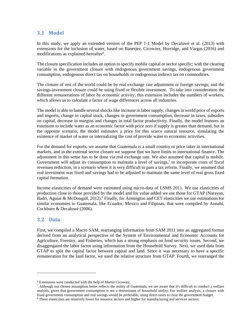
The first step was to construct a Macro SAM using information from Escobar’s SAM for 2011. Also, weidentified accounts that could be disaggregated using supply and use tables from BANGUAT.

Table 2 - Macro SAM (in millions of Quetzales)

L K AG AG AG AG AG AG AG AG J I OTH OTHLAB CAP HH GVT ROW TACT TI TM TD TFAC A C INV VSTK TOTAL

L LAB 871191,64

0192,51

1

K CAP 502153,75

6154,25

9

AG HH181,58

4142,85

611,99

3 34,805371,23

7

AG GVT 50 2,721 2,2002,26

120,82

92,52

413,19

910,84

6 54,630

AG ROW 82 11,353 262 97138,60

5150,39

9AG TACT 2,261 2,261AG TI 20,829 20,829AG TM 2,524 2,524AG TD 13,199 13,199AG TFAC 10,846 10,846

J A594,17

0594,17

0

I C316,52

837,80

3 98,783246,51

254,91

01,59

2756,12

9OTH INV 38,526 4,738 13,238 56,502OTH VSTK 1,592 1,592

TOTAL

192,511154,25

9371,23

754,630150,39

92,26120,8292,52413,19910,846594,17

0756,12

956,5021,592

Source: own construction.

Then we disaggregated the labor factor between skilled (L-SKL) and unskilled (L-UNS)10 labor. Weapplied the GTAP relative structure on remunerations for Capital, Land and Natural Resources11.Furthermore, we split gross operating surplus by activity. As a result, the final size of the SAM is of 8activities and 32 commodities12. Based on information from a processed SUT13, we proceeded to divideremunerations of labor, production, and intermediate consumption by activity.

Using the Living Standards Measurement Survey, we split the accounts to match our household structure.In this exercise we classified them in four types: rural poor, rural non-poor, urban poor, and urban non-poor. Poverty was determined using the official poverty line of 201114 and, using information from thehousehold survey, we were able to estimate labor income, consumption and most transfers15 accordingto each type of household.

9 The SAM used in this study was constructed using three sources of information: SAM 2011 (Escobar, 2015), Supply and UseTables (SUT) from the Central Bank of Guatemala (BANGUAT) for the year 2011, the relative structure of remunerations ofcapital and land found on the GTAP model, and the Life Standards Measurement Survey (Encovi in Spanish) from the year2011 (INE, 2011). See annex 7.1 for detail of the construction of the SAM.10 Skilled workers are those with 9 years of schooling or more.11 Narayanan, G., Badri, Angel Aguiar and Robert McDougall (2012).12 See activities included in SAM in annex 7.1.13 We collapsed activites from SUT from BANGUAT (2014) to create an Ad-hoc SUT.14 See Living Standards Measurement Survey, INE (2011).15 Transfers from Government and Rest of the world

Savings were estimated as a residual from factor income, as well as transfers from government and therest of the world, minus transfers to Government, and transfers to the rest of the world and consumption.Using the processed SUT we included in the SAM all exports by commodity, intermediate consumption,supply, investment, and margins of trade and transport.

3.3 Guatemala’s economic structure

The Social Accounting Matrix allows us to describe how the Guatemalan economy is structured. Weconsider that this description is important to understand the impact of the various shocks that we haveconducted in this study.

3.3.1 Main productive sectors

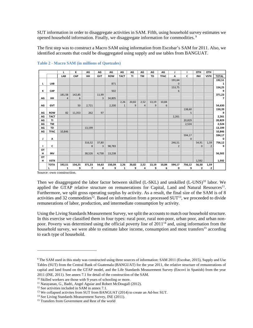
Services create more value added than other economic activities, with 65.1% of the total. Industryconstitutes 20% of the remaining value added, out of which over 50% is related to the food processingindustry. Agriculture activities, animal production, forestry and fishing account for 11.9% of the addedvalue, of that percentage, the majority is represented by agriculture, with 8.7%. Activities under “otherprimary activities16” represent 3.0% of the total value added.

Table 3 - Added value per sector (millions of Quetzales and percentage)

Sectors VA %

Agriculture 29,906.3 8.7

Animal production 7,268.9 2.1

Forestry and fishing 3,831.4 1.1

Other primary activities 10,505.5 3.0

Food and beverage products 36,714.7 10.6

Other manufacturing industries 32,190.9 9.3

Services 224,979.1 65.1

Total 345,396.8 100.0Source: Social Accounting Matrix for Guatemala, 2011.

3.3.2 Activities focused on the external sector

Most of the exports are food products (36.1%), other industries at 15.4%, and other forestry productswith 9.9% of the exports. On the agricultural side, coffee and bananas are 9.2% and 3.7% of the exports,followed by vegetables at 3.8% and fruits at 1.8%. The export percentage column in Table 4 below showsthat 68% of the coffee output is exported, and that number is 40.2% for bananas, 79% for other animalproducts, 65.8% for prepared or preserved fish, 56% for preparation used in animal feeding, and 55.9%for food products.

On the imports side, the “Other Industries” category accounts for 80.2%, and “Other Services” accountsfor 6.3%. Agricultural products account for less than 5%, with maize at 1.3%. Most of nationalconsumption of cereals, at 67.8%, is imported. The “Other Industries” category shows 50.5% isimported, and 43.2% is imported for animal and vegetable oils and fats. Due to the importance of maizein the Guatemalan diet, it’s important to emphasize that 15.2% of the national consumption is imported.

16 Other primary activities include extractive industries like mining and oil extraction.

Table 4 - Exports and imports by commodity (in percentage)

Commodities Exports% Exportproduction Imports

%Imports

Coffee 9.2 68.0 0.0 0.0Bananas 3.7 40.2 0.0 0.1Maize 0.1 0.2 1.3 15.2Beans 0.0 0.2 0.1 2.7Cereal and legumes 0.0 0.2 1.2 67.8Roots and tuberous vegetables 0.1 0.7 0.0 0.5Other vegetables 3.8 8.1 0.0 0.3Other fruits 1.8 16.0 0.3 6.5Living plants 1.2 13.7 0.7 11.9Milk 0.0 0.3 0.0 0.0Eggs 0.0 0.7 0.0 1.1Other animal products 3.4 79.0 0.0 0.0Firewood 0.6 10.2 0.0 0.0Other forestry and loggingproducts

9.9 42.5 0.2 1.1

Fish and fishery products 0.4 23.1 0.1 10.9Other minerals 0.3 4.8 0.7 23.5Meat and meat products 0.8 3.7 0.7 5.5Prepared or preserved fish 2.7 65.8 0.2 9.5Prepared and preserved vegetables 0.3 11.7 0.6 31.9Animal and vegetable oils and fats 0.3 4.3 1.9 43.2Grain mill products 0.6 2.8 0.8 7.1Preparation used in animal feeding 5.5 56.0 0.2 4.1Bakery products 0.2 0.6 0.5 2.5Sugar 0.1 1.0 0.0 0.1Noodles and similar farinaceousproducts

2.1 43.5 0.1 2.6

Dairy products 0.9 6.9 0.8 11.8Food products n.e.c. 36.1 55.9 2.2 6.6Alcoholic and non-alcoholicbeverages

0.2 4.0 0.3 8.7

Other industries 15.4 6.9 80.2 50.5Water and electricity 0.0 0.0 0.4 3.9Lodging 0.0 0.0 0.0 0.0Other services 0.0 0.0 6.3 2.7

Source: Social Accounting Matrix for Guatemala, 2011.

3.3.3 Employment structure and earnings

Table 5 shows that 55.5% of the value added is allocated to labor (29.1% skilled and 26.4% unskilled),41.9% to capital, 2% to land and 0.6% to natural resources. When looking at the details, over 58% of theparticipation across agriculture, animal products and forestry and fishing activities is unskilled labor,followed to a much smaller degree by capital and land. For other primary activities, the participation ofcapital represents 48.7% of added value, unskilled labor, 25.2%, natural resources, 19% and skilled labor,less than 10%.

On the food industry sector, the majority of the added value is allocated to skilled labor, at 37.4%, withcapital following closely at 35.5%, and lastly by unskilled labor at 27%. On other services sector, capital

is the largest percentage of the added value at 47%, followed by skilled labor at 33.7% and unskilledlabor at 19.4%.

Table 5 - Factorial composition of value added (percentage)

SectorsLabor

Capital LandNatural

resourcesTotal

Skilled Unskilled

Agriculture 6.8 61.7 14.9 16.6 0.0 100

Animal production 6.5 59.4 16.1 18.0 0.0 100

Forestry and fishing 6.8 58.9 16.2 18.2 0.0 100

Other primary activities 7.1 25.2 48.7 0.0 19.0 100

Food industry 37.4 27.0 35.5 0.0 0.0 100

Other manufacturing industries 23.4 30.8 45.8 0.0 0.0 100

Other services 33.7 19.4 47.0 0.0 0.0 100

Total 29.1 26.4 41.9 2.0 0.6 100Source: Social Accounting Matrix for Guatemala, 2011.

3.3.4 Household income

Non-poor households in urban areas account for 71.1% of the total income, while non-poor householdsin rural areas account for 11.6%. The remaining 17.3% of the total income is accounted by poorhouseholds, 9.8% in rural areas and 7.5% in urban areas.

Table 6 shows the distribution of income for each household group. It is important to highlight that mostof the labor income of skilled workers corresponds to non-poor households in urban areas (83.4%), andvery little corresponds to non-poor rural households (9.0%). However, it can be seen that unskilled laboris distributed across all household groups, especially non-poor urban ones.

For the capital income category, 95.3% corresponds to non-poor urban households, 3.4% to poor urbanhouseholds, and less than 2% to households in rural areas. More than 50% of land income correspondsto non-poor households, 48.3% to rural areas and 2.7% to urban areas, while the remaining 49% isdistributed across poor households, in very similar proportion. For natural resources, 72.1% correspondsto non-poor households in urban areas and 13% to non-poor households in rural areas. Almost 15% ofthe remaining corresponds to poor households.

Table 6 - Distribution of income for each household group (percentage)

Household groupLabor

Capital LandNatural

resourcesSkilled Unskilled

Urban poor 4.9 15.6 3.4 25.0 8.8

Rural poor 2.7 26.9 0.2 24.0 6.1

Urban non-poor 83.4 36.9 95.3 2.7 72.1

Rural non-poor 9.0 20.6 1.2 48.3 13.0

Total 100.0 100.0 100.0 100.0 100.0Source: Social Accounting Matrix for Guatemala, 2011.

Table 7 shows income composition for each household group. For poor households in urban areas, 47.9%of their income corresponds to unskilled labor, followed in similar proportion by skilled labor (16.9%)and capital (16.2%). Transfers from the rest of the world accounted for 8.1% of their income.

For poor households in rural areas, unskilled labor income represents the highest proportion of theirincome (63.4%), followed by transfers from the rest of the world (15.8%) and government transfers(8.2%). For non-poor rural households, labor income accounted for 61% of revenues, 41% for unskilledand 20% for skilled labor. For this group of households, transfers from the rest of the world representjust under a quarter of their income.

For non-poor households living in urban areas, capital income represents almost half their income, andin less proportion, labor income accounts for 42.3%, as well as 30.3% for skilled labor and 12% forunskilled workers. Transfers from the rest of the world accounted for 6.3% of their income, andgovernment transfers, for 2.5%.

It is important to note that although government transfers and transfers from the rest of the worldrepresent a smaller proportion of the income of non-poor urban households, in absolute terms income ishigher in this group of households.

Table 7 - Income composition for each household group (Percentage)

Householdgroup

LaborCapital Land

Naturalresources

Governmenttransfers

TransfersRoW

Skilled Unskilled

Urban poor 16.9 47.9 16.2 6.3 0.6 4.0 8.1

Rural poor 7.0 63.4 0.6 4.6 0.3 8.2 15.8

Urban non-poor 30.3 12.0 48.3 0.1 0.5 2.5 6.3

Rural non-poor 20.0 41.0 3.7 7.8 0.6 3.2 23.6

Source: Social Accounting Matrix for Guatemala, 2011.

3.3.5 Household consumption

Non-poor households from urban areas accounts for 59.5% of national consumption, and non-poor ruralhouseholds, just under a fifth (18.1%). While consumption of poor household’s accounts for 22.4% ofdomestic consumption, 7.8% for households in urban areas and 14.6% in rural areas (see table 19 inannex 7.2).

It appears that for poor households, food accounts for the largest share of consumption, mainly for poorrural households, food accounts for 62.1% of its consumption. In table 19, we can see that for these poorrural households, beans and corn account for more than 10% of its consumption.

For non-poor households, the proportion of food consumption is lower, specifically for non-poorhouseholds in urban areas, where it represents less than a third (31.1%) of total consumption. For thissame group, services account for 44.8% of consumption. It is important to note that, although for non-poor households in urban areas the proportion of consumption in corn and beans is less than for poorrural households, 3% compared to 11.5%, in absolute terms, the consumption of corn and bean in non-poor households in urban areas is higher than in poor rural households.

4 Application and results

4.1 Results from simulations

In this section we present the results from simulating a) a reduction in productivity due to climate change;and b) the effects of drought in agriculture.17

In first scenario, we take into consideration likely effects of climate change in grains. This effect couldbe caused by changes in mean temperature, variability of climate and extreme events, water availability,mean sea-level rise, pest and diseases (Gornall et al., 2010). There is no consensus about clear effects onagriculture on Guatemala, but we assume a negative scenario according to ECLAC, in one scenario ofclimate change, production of grains in year 2020 could be reduced around 8% in maize, beans andwheat. So, we estimate a scenario where total factor productivity of agriculture for food and agriculturefor seed drops around 8%.

A specific scenario of environmental shock is when a drought occurred. Using information of waterconsumption by economic activity, we estimate likely effects of a drought that reduce in 25% the stockof water. Because information about total supply of water are not available in Guatemala, we assumethat total demand is close to 90% of total supply. We also don’t know what will be the exact orapproximate change in price of water, because Guatemala does not have a market of this natural resource.However, the results give us an idea of likely effects of droughts in economic activity.

4.1.1 Reduction in productivity due to climate change

As we mentioned before, climate change could have negative effects in agriculture productivity. Underthis scenario we estimate negative results in production, exports, wages and reduction of governmentrevenues, which should result in a decrease in spending (consumption). Besides negative effects of foodsecurity due to the diminished production and consumption of agricultural goods, our figures show thatthe effects of climate change could increase inequality, because the wages of unskilled labor would seea reduction as a result of an increase of capital income and skilled labor wages.

In this case, we registered an important drop in the value added of agriculture and animal production aswell as a slight drop in that of industrial food production and the service industry. It is important to takeinto consideration that in this scenario we observed a fall in real GDP (1.2%), as can be seen in Table 8.Those products that are oriented to international markets show a decrease, because goods like maize,bean, root and tuberous vegetables have a lower fall rate compared with coffee, bananas and fruits. Thisis explained by the fact that lower productivity would translate into less competitiveness in internationalmarkets. Exports in real terms fell by 2.0%, but also we observed a decrease in imports of 1.5% in realterms. It is important to note that a depreciation of the real exchange rate contributed to the reduction ofthe negative impacts on external sectors. Another problem that we could see with reduction ofproductivity is that fiscal space was reduced. As an effect, government expenditure had to be reduced inview of lower tax revenues. There was also less income of households and less consumption.

17 The sensitivity results are included in annex 7.3.

Table 8 - GDP table (% change)

Real GDP shareAbsorption -1.1 0.2Private Consumption -1.4 0.2Fixed Investment 0.0 0.9Stock Change 1.8Government Consumption -0.6 -0.3Exports -2.0 0.6Imports -1.5 1.1GDPMP -1.2 0.0NetIndTax 0.1GDPFC -1.2 0.0

Source: own calculations.

Figure 1 - Aggregate output by industry in scenario of decrease of TFP (% change)

Source: own calculations.

Due to higher prices and lower income of households, lower productivity translates into a drop inconsumption of agricultural goods for each type of household. The exception was Maize, because itsdemand was covered by imports and their consumption only fell in rural areas, besides, in urban areasthis product is perfectly inelastic (zero elasticity). However, the results of this scenario could affect foodsecurity of the most vulnerable population of Guatemala. Beans, which are also important for theGuatemalan diet, showed a decrease in consumption for all types of households. This behavior is notonly the result of higher prices, but also of because of a decrease in household incomes for all categories;especially the urban non-poor (1.5%). Wages of unskilled labor fell less because Forestry and Fishingincrease their production and could absorb excess labor from animal production. Another cause is thateven though production fell in agriculture, to satisfy domestic demand it was necessary to hire moreemployees in agriculture, because employment in agriculture rise.

Table 9 - Agricultural goods: Price and consumption by household type (% change)

Coffee Bananas Maize Beans Cereals Roots&Tubers

Vegetables Fruits Processedfood

Others

Price 5.3 9.3 3.2 4.4 1.6 4.0 2.9 3.9 0.7 -0.1

Consumption by type of household

Urban Poor -1.8 -2.3 0.0 -0.8 -1.8 -2.0 -1.9 -2.1 -1.2 -1.3

Rural Poor -1.5 -1.9 -1.1 -1.1 -1.6 -1.9 -1.7 -1.7 -0.8 -1.1

Urban Non Poor -2.1 -2.8 0.0 -0.9 -2.1 -2.3 -2.3 -2.4 -1.6 -1.8

Urban Poor -1.3 -1.8 -0.8 -0.9 -0.9 -1.5 -1.4 -1.4 -0.2 -0.2

Source: own calculations.

We observed a deterioration of the external sector. First, we identified a sharp drop in exports, especiallyin cereals, maize, fruits, vegetables, coffee and banana. Because local prices were higher, some of them

-7.8

-13.1

24.9

6.2

-0.9

0.0

-0.9

-20.0 -10.0 0.0 10.0 20.0 30.0

Agriculture

Animal Production

Forestry & Fishing

Other primary activities

Industrial Food

Other Industries

Services

were replaced by imports, like maize and banana. This situation, however, was moderated by adepreciation of the real exchange rate, in order to sustain the same level of deficit in the current account.

4.1.2 Effects of drought on agriculture

This version of PEP 1-1 Model contains an extension made by Banerjee et al. (2016) to analyze effectsof shortage of supply of water or drought. We analyze the effects on agricultural industries. In thisscenario, agricultural sectors, which use this resource more intensely, were the most affected. Due to thefact that the use of water is concentrated in agriculture and forestry and fishing (see next figure), mostnegative effects are concentrated in these industries. In contrast, other economic activities that did notuse water as an important input would not be affected. Another important effect was the climb in foodprices, the reduction of wages of unskilled labor, and the reduction of income for rural households. TheGDP rise in this scenario because this shock doest not has a negative impact on other industries andservices, that pay higher remunerations that sectors affected.

Figure 2 - Water use by industry (% total)

Source: own calculations based on INE et al. (2013).Note: includes use of registered and unregistered water as explained in document cited above.

Private consumption remained almost unchanged. This was closely linked to the reduction in disposableincome of the urban non-poor households; a group responsible for more than 70% of total householdconsumption. And although labor income saw a reduction in all kinds of households, it fell only 4.7%for the urban non-poor, in contrast to more than 5% for the other categories.

Table 10 - GDP table (% change)

Real GDP share

Absorption 0.7 0.3Private Consumption 0.3 0.7Fixed Investment 0.0 -2.6Stock Change 0.0Government Consumption 5.8 0.9Exports 0.5 5.0Imports -0.1 4.5GDPMP 1.0 0.0GDPFC 1.4 -4.7

Source: own calculations.

59%21%

15%1%

Agriculture Animal Products Forestry & Fishing

Other primary activities Industrial Food Other Industries

Services Households

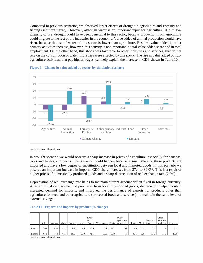
Compared to previous scenarios, we observed larger effects of drought in agriculture and Forestry andfishing (see next figure). However, although water is an important input for agriculture, due to lowintensity of use, drought could have been beneficial to this sector, because production from agriculturecould migrate to the rest of the industries in the economy. Value added of animal production would haverisen, because the use of water of this sector is lower than agriculture. Besides, value added in otherprimary activities increase, however, this activity is not important in total value added share and in totalemployment. On the other hand, this shock was favorable to other industries and services, that do notrely on the consumption of water. Industries were affected by this shock. The rise in value added of non-agriculture activities, that pay higher wages, can help explain the increase in GDP shown in Table 10.

Figure 3 - Change in value added by sector, by simulation scenario

Source: own calculations.

In drought scenario we would observe a sharp increase in prices of agriculture, especially for bananas,roots and tubers, and beans. This situation could happen because a small share of these products areimported and have a low degree of substitution between local and imported goods. In this scenario weobserve an important increase in imports, GDP share increases from 37.4 to 39.0%. This is a result ofhigher prices of domestically produced goods and a sharp depreciation of real exchange rate (7.0%).

Depreciation of real exchange rate helps to maintain current account deficit fixed in foreign currency.After an initial displacement of purchases from local to imported goods, depreciation helped containincreased demand for imports, and improved the performance of exports for products other thanagriculture for seed and other agriculture (processed foods and services), to maintain the same level ofexternal savings.

Table 11 - Exports and imports by product (% change)

Coffee Bananas Maize Beans Cereals

Roots&Tubers Vegetables Fruits

Otheragricultureproducts Mining Meat

Industrialfoods

Otherindustrialproducts Services

Import 30.6 43.9 41.1 8.9 7.9 20.9 5.1 19.1 10.8 3.0 3.5 3.3 1.6 3.5

Exports -64.5 -44.0 -66.7 -18.9 -66.9 -71.5 -65.3 -69.9 -6.7 46.1 -5.4 13.3 11.7 10.4

Source: own calculations.

-7.1 -7.8

12.7

4.4

-0.8

0

-0.9

-23.4

19.7

-19.3

27.5

3.27.8

1.7

-30

-20

-10

0

10

20

30

40

Agriculture AnimalProduction

Forestry &Fishing

Other primaryactivities

Industrial Food OtherIndustries

Services

Climate Change Drought

5 Lessons learned, innovations and policy implications

Even though the long term development plan was presented in 2014, policy makers need evidence-basedresearch to fill the information gaps in order to implement it. For example, there is consensus that climatechange is an imminent risk for the country's development, but there were few insights to anticipate theimpact of these weather events.

Guatemala is one of the few countries in the world that has an updated System of Environmental andEconomic Accounts. However, there are not so many studies that take advantage of this information totranslate into policy recommendations. For that reason, this is one of the first studies to use this data –together with the System of National Accounts from the Central Bank– to inform policy actions towardsthe mitigation and adaptation to climate change.

As it is known, low latitude countries, like Guatemala, are prone to face warmer temperatures in thefuture decades. Several scientists have projected by how much temperature will rise and this translatesinto hotter and more frequent hot days in the countries located in those regions. However, rather thanexplaining how temperature will vary, policy makers need information to acknowledge the effects of dryspells.

As a result, we were willing to explore the impact that droughts –expressed by a reduction of waterstocks– would have in growth, remunerations and food security. One of the findings refers to the declineon the value added created by agriculture (value added would decrease by 23%). As expected, thissituation negatively affected the wages paid to unskilled workers, but also urban non-poor householdswould saw a reduction of their disposable income due to higher food prices. Thus, there is no segmentof society that would not be affected.

Moreover, one of the most interesting results is that under a drought scenario the demand for land wouldfall down by 38 per cent. This is because as water would become scarcer, there would be fewer incentivesto engage in agricultural activities. However, due to the importance of agricultural production forensuring food security, this results show that a proper water allocation system is needed.

Guatemala cannot postpone the creation of a legal framework to govern water resources. For that, wecould consider the experience of Australia that has historically suffered megadroughts so this countryhas reformed its water allocation system. At first, an agreement between the federal and stategovernments was reached (National Water Initiative, 2004) to create a national water market. The ideabehind this allocation system is that “water entitlements are expressed as a share of the available resourcerather than as a specified quantity of water” (Peel & Choy, 2014).

In short, despite of the existence of an National Irrigation Policy in Guatemala, the framework isincomplete since there is not a water allocation system that prioritizes strategic economic activities toguarantee food security.

The other simulation that was applied is also related to climate change, but we were more specific. Wesimulated a reduction in agricultural productivity, and one of the main results refer to the sharp drop inexports, especially in cereals, maize, fruits, vegetables, coffee and banana. This means that the countrywould be less competitive to sell agricultural products overseas. This would have large implications onpursuing an export-led growth strategy.

6 References

Alexandratos, N. & Bruinsma, J. (2012). World agriculture towards 2030/2050: the 2012 revision. ESAworking paper, 12(03).

Amsden, A. (2001). The Rise of “The Rest”: Challenges to the West from Late-IndustrializingEconomies: Challenges to the West from Late-Industrializing Economies. Oxford University Press.

Annabi, N., Cockburn, J. & Decaluwé, B. (2006). Functional Forms and Parametrization of CGE Models.MPIA Working Paper 4. Retrieved from http://portal.pep-net.org/documents/download/id/13525

Antle, J. M., & Capalbo, S. M. (2010). Adaptation of Agricultural and Food Systems to Climate Change:An Economic and Policy Perspective. Applied Economic Perspectives and Policy , 32 (3), 386-416.

Banerjee, O. Cicowiez, M., Horridge, M., and Vargas, R. (2016) A Conceptual Framework for IntegratedEconomic-Environmental Modeling. Journal of Environment & Development, 25(3), 276-305.

Bourguignon, F., Bussolo, M. & Pereira da Silva, L. (2008). The Impact of Macroeconomic Policies onpoverty and income distribution. Macro-Micro evaluation techniques and tools. Palgrave Macmillanand the World Bank, New York and Washington, D.C.

Cabrera, M. and Delgado, M. (2010). Implicaciones de la política macroeconómica, los choques externosy los sistemas de protección social en la pobreza, la desigualdad y la vulnerabilidad en AméricaLatina y el Caribe. Guatemala. CEPAL, 2010.

Cicowiez, M. and Sanchez, M. (2010). Choques externos y Políticas de Protección Social en AméricaLatina. Documento de Trabajo Nro. 105. Cedlas, Universidad de la Plata, Argentina.

Cline, W. (2007). Global Warming and Agriculture: Impact Estimates by Country. Washington DC:Center for Global Development, Peterson Institute for International Economics.

Comisión Económica para América Latina y El Caribe. (2013). Impactos potenciales del cambioclimático sobre los granos básicos en Centroamérica. México DF.

CONADUR/SEGEPLAN (2014). Plan Nacional de Desarrollo K’atun: nuestra Guatemala 2032.Consejo Nacional de Desarrollo Urbano y Rural; Secretaría de Planificación y Programación de laPresidencia, Guatemala.

Conforti, P. (2011). Looking ahead in world food and agriculture: perspectives to 2050. Rome: Foodand Agriculture Organization.

Decreaux, Y. & Valin, H. (2007). MIRAGE, Updated Version of the Model for Trade Policy Analysis.Focus on Agriculture Dynamics.

Dervis, K., De Melo, J. & Robinson, S. (1982). General Equilibrium Models for Development Policy.Cambridge: Cambridge University Press.

Economist Intelligence Unit. (2014). Food security in focus: Central and South America 2014. TheEconomist.

Escobar, P. (2015). Efectos distributivos de las vulnerabilidad externas en Guatemala, Tesis de Maestríaen Economía. Universidad Nacional de La Plata, Argentina.

FAO (2015). Regional Overview of Food Insecurity, Latin America and the Caribbean. Santiago deChile: FAO.

FAO (2008). Climate change: Implications for Food Safety. Rome: FAO. Retrieved fromhttp://www.fao.org/docrep/010/i0195e/i0195e00.HTM

FAO (n/d). System of Environmental and Economic Accounts for Agriculture, Forestry and Fisheries.Rome: Food and Agricultural Organization of the United Nations. United Nations StatisticalDivision. Retrieved from: http://unstats.un.org/unsd/envaccounting/aff/chapterList.asp

Gornall, J., Betts, R., Burke, E., Clark, R., Camp, J. Willet, J. & Wiltshire, A. (2010), “Implications ofclimate change for agricultural productivity in early twenty-first century”, Philosophical transactionsof the Royal Society B, September 2010, Volume 365 Issue 1554.

Hallegatte, S., Bangalore, M., Bonzanigo, L., Fay, M., Kane, T., Narloch, U., et al. (2016). Shock Waves:Managing the Impacts of Climate Change on Poverty. Washington DC: The World Bank. Retrievedfrom http://hdl.handle.net/10986/22787

Iarna, IICA & McGill University (2015), “Food insecurity and under-nutrition in Gautemala”. FinalReport. Guatemala.

Iarna-URL/FAUSAC (2013). Evaluación del Programa de Fertilizantes del Ministerio de Agricultura,Ganadería y Alimentación (MAGA). Instituto de Agricultura, Recursos Naturales y Ambiente,Universidad Rafael Landívar; Facultad de Agronomía, Universidad de San Carlos de Guatemala.Guatemala.

INE (2002). Censos Nacionales, XI de Población y VI de Habitación, 2002. Guatemala.

INE (2011). Encuesta Nacional de Condiciones de Vida 2011 [Data file]. Retrieved fromhttps://www.ine.gob.gt

INE, Banguat y Iarna-URL (2013). Sistema de Contabilidad Ambiental y Económica de Guatemala2001-2010, SCAE 2001-2010. Tomo I. Guatemala.

Instituto Nacional de Bosques / Programa Forestal Nacional [INAB/PFN] (2013). Ley de Fomento alestablecimiento, recuperación, restauración, manejo, producción y protección de bosques enGuatemala – PROBOSQUE. Guatemala: Secretaría Técnica del Instituto Nacional de Bosques.

International Food Policy Research Institute. (2016). Food policy in a complex, changing world. Eventsynopsis. Washington DC.

Kreft, S., Eckstein, D., Dorsch, L., & Fischer, L. (2015). Global Climate Risk Index 2016. Bonn:Germanwatch.

Llop Llop, M. & Ponce, X., 2011. "A never-ending debate: Demand versus supply water policies. ACGE analysis for Catalonia" Working Papers 2072/152139, Universitat Rovira i Virgili, Departmentof Economics.

Lofgren, H. Cicowiez, M. and Diaz-Bonilla, C. (2013). MAMS – A Computable General EquilibriumModel for Developing Country Strategy Analysis. In: Dixon, P.B., Jorgenson, D.W. (Eds.),Handbook of Computable General Equilibrium Modeling. North Holland, Elsevier B.V., pp. 159–276.

Lofgren, H. Lee Harris, R. & Robinson, S. (2002). A Standard Computable General Equilibrium (CGE)Model in GAMS. International Food Policy Research Institute (IFPRI) Microcomputers in PolicyResearch 5.

Ministerio de Agricultura, Ganadería y Alimentación [MAGA] (2013). Política de Promoción del riego2013-2023. Guatemala.

Narayanan, G., Badri, Angel Aguiar and Robert McDougall, Eds. (2012). Global Trade, Assistance, andProduction: The GTAP 8 Database [Data file]. Center for Global Trade Analysis, Purdue University.

Peel, J., & Choy, J. (2014). Water Governance and Climate Change. Stanford: Water in the West,Stanford University.

Robles M. & Keefe, M. (2011), “The effects of changing food prices on welfare and poverty inGuatemala”, Development in Practice 21(4-5): 578-589.

Rosegrant, M., Koo, J., Cenacchi, N., Ringler, C., Robertson, R., Fisher, M., Sabbagh, P. (2014). FoodSecurity in a World of Natural Resource Scarcity, The Role of Agricultural Technologies.Washington DC: International Food Policy Research Institute.

Silvia Saravia-Matus, Sergio Gomez y Paloma, and SébaStien Mary (2012). “Economics of FoodSecurity: Selected Issues”. Bio-based and Applied Economics 1(1): 65-80.

Silvia Saravia-Matus, Sergio Gomez y Paloma, and SébaStien Mary (2012). “Economics of FoodSecurity: Selected Issues”. Bio-based and Applied Economics 1(1): 65-80.

Smith, L.C., El Obeid, A.E. and Jensen, H.H. (2000). The Geography and Causes of Food Insecurity inDeveloping Countries. Agricultural Economics 22: 199-215.

Smith, L.C., El Obeid, A.E. and Jensen, H.H. (2000). The Geography and Causes of Food Insecurity inDeveloping Countries. Agricultural Economics 22: 199-215.

Tirado, M., Clarke, R., Jaykus, L., McQuatters-Gollop, A., & Frank, J. (2010). Climate change and foodsafety: A review. Food Research International , 43 (7), 1745-1765.

Tomlinson, I (2011). Doubling Food Production to Feed the 9 Billion: A Critical Perspective on a KeyDiscourse on Food Security in the UK. Journal of Rural Studies. doi:10.1016/j.jrurstud.2011.09.001.

Tomlinson, I (2011). Doubling Food Production to Feed the 9 Billion: A Critical Perspective on a KeyDiscourse on Food Security in the UK. Journal of Rural Studies.

Torero, M. & Robles, M. (2010). Understanding the Impact of High Food Prices in Latin America.Economía, 10(2), 117-164.

UNDP (2012). Guatemala: ¿un país de oportunidades para la juventud?. Informe Nacional de DesarrolloHumano, UNDP Guatemala.

UNESCO (2013). Global water resources under increasing pressure from rapidly growing demands andclimate change, according to new UN World Water Development Report. UNESCOPRESS.

UNESCO-IHP, WMO, & IAHS. (2016). Climate change and extreme events. In UNESCO, Water andjobs (pp. 24-29). Paris: United Nations Educational, Scientific and Cultural Organization.

United Nations. (2015). The Millenium Development Goals Report 2015. New York: Department ofEconomic and Social Affairs .

United Nations. (2016). Millennium Development Goals Indicators. Retrieved from http://mdgs.un.org/

Vásquez, W. (2008). Guatemala. In: Vos, R., Ganuza, E., Lofgren, H., Sánchez, M.V., Díaz-Bonilla, C.(Eds) (2008). Políticas Públicas para el Desarrollo Humano: ¿Cómo lograr los Objetivos deDesarrollo del Milenio en América Latina y el Caribe? Uqbar and UNDP. UNDP, UN-DESA andWorld Bank, Washington, DC, pp. 451-476.

Vos, R. andSánchez, M. (2010). A Non-Parametric Microsimulation Approach to Assess Changes inInequality and Poverty. International Journal of Microsimulations 94.

Wissema, W. & Dellink, R. (2007). AGE analysis of the impact of a carbon energy tax on the IrishEconomy. Ecological Economics, 61(4), 671-683.

World Food Program (2011). 11 Myths About Global Hunger. Retrieved fromhttps://www.wfp.org/stories/11-myths-about-global-hunger

World Summit on Food Security (2009). Declaration of the World Summit on Food Security. Rome 16-18 November 2009.

World Summit on Food Security (2009). Declaration of the World Summit on Food Security. Rome 16-18 November 2009.

Yu, B., You, L., & Fan, S. (2010). Toward a Typology of Food Security in Developing Countries. IFPRIDiscussion Paper 945.

7 Annex

7.1 Constructing of the Social Accounting Matrix for Guatemala

7.1.1 Sources of Information

The SAM was constructed using three sources of information: SAM 2011 (Escobar, 2015), Supply andUse Tables (SUT) from the Central Bank of Guatemala for the year 2011, the relative structure ofremunerations of capital and land found on the GTAP model, and the Life Standards MeasurementSurvey (Encovi) from the year 2011 (INE, 2012). Since the SAM for year 2011 (Escobar, 2015 that wehad as a starting point does not conform to the requirements of the PEP 1-1 model and also does not havethe necessary degree of disaggregation of activities, commodities and households to analyze impacts ofagricultural incentive policies on socioeconomic and environmental variables in Guatemala, the NationalAccounts’ SUT for the year 2011 were used to disaggregate agricultural activities and commodities, aswell as activities with high demand of water. In order to estimate the relative structure of factorremunerations by activity, transfers to households, and consumption by household, the household surveywas used to derive standard coefficients.

7.1.2 Constructing the national social accounting matrix

Six steps were taken for the construction of a suitable SAM Guatemala 2011 for this study. First, wecompiled a Macro SAM, rearranging information from SAM 2011 into an aggregated format derivedfrom an analytical perspective of the System of Environmental and Economic Accounts for Agriculture,Forestry, and fisheries, which has a strong emphasis on food security issues. Second, we disaggregatedthe labor factor using information from the Household Survey. Next, we used data from GTAP to splitthe capital factor between capital and land. Since it was necessary to have a specific remuneration forthe land factor, we used the relative structure from GTAP. Fourth, we rearranged the SUT informationin order to disaggregate activities in SAM. Fifth, using household survey estimates we opened householdinformation. Finally, we opened information for commodities.

The first step was to construct a Macro SAM using information from Escobar’s SAM (2011). Also, weidentified accounts that could be disaggregated using supply and use tables from the central bank ofGuatemala (BANGUAT).

Table 12 - Macro SAML K AG AG AG AG AG AG AG AG J I OTH OTHLAB CAP HH GVT ROW TACT TI TM TD TFAC A C INV VSTK TOTAL

L LAB 871191,64

0192,51

1

K CAP 502153,75

6154,25

9

AG HH181,58

4142,85

611,99

3 34,805371,23

7

AG GVT 50 2,721 2,2002,26

120,82

92,52

413,19

910,84

6 54,630

AG ROW 82 11,353 262 97138,60

5150,39

9AG TACT 2,261 2,261AG TI 20,829 20,829AG TM 2,524 2,524AG TD 13,199 13,199AG TFAC 10,846 10,846

J A594,17

0594,17

0

I C316,52

837,80

3 98,783246,51

254,91

01,59

2756,12

9OTH INV 38,526 4,738 13,238 56,502

OTH VSTK 1,592 1,592

TOTAL

192,511154,25

9371,23

754,630150,39

92,26120,8292,52413,19910,846594,17

0756,12

956,5021,592

Source: Own construction.

Then we disaggregated the labor factor between skilled (L-SKL) and unskilled (L-UNS)18 labor. BecauseEscobar’s SAM has four different labor factors (wage skilled, non-wages skilled, wage unskilled, non-wag) we used the relative structure to estimate L-SKL and L-UNS.

We applied the G-TAP relative structure on remunerations for Capital, Land and Natural Resources19.Furthermore, we split gross operating surplus by activity. Based on information from a processed SUT20,we proceeded to divide remunerations of labor, production, and intermediate consumption by activity.Because we don’t have disaggregation of transfers (non-tax) from activities to government and taxes onactivities, we estimated those as a residual.

The SAM includes three types of agents, households, government and rest of the world. The PEP 1-1model includes a set for “enterprises”, but since we did not have access to information on transfersbetween enterprises and different type of households, we chose not to include them.

Using the Life Standards Household Survey, we split the accounts to match our household structure. Inthis exercise we have four types of households: rural poor, rural non-poor, urban poor and urban non-poor. Poverty was determined using the official poverty line of 201121 and, using information from thehousehold survey, we were able to estimate labor income, consumption and most transfers22 accordingto type of household. Savings were estimated as a residual from factor income, as well as transfers fromgovernment and the rest of the world, minus transfers to Government, and transfers to the rest of theworld and consumption.

Finally, using data from the household survey we created a split by commodity accounts. These accountsinclude consumption by household. Using the processed SUT we included in the SAM all exports bycommodity, intermediate consumption, supply, investment, and margins of trade and transport. To closethe SAM, we estimated residually the change in inventories from two activities (beverages and otherindustries).

7.1.3 Activities and Commodity aggregations of Supply and Use tables

In order to improve the analytical potential of the SAM, we turned to the recently drafted manual for theSystem of Environmental and Economic Accounts for Agriculture, Forestry, and Fisheries (FAO, n/d),which has a strong emphasis on food security issues. The logic behind the aggregation of economicsectors and commodities proposed by the manual implies that there are some crops that are used by someindustries mainly for animal feed and other industries as seed. Some manufacturing industries then useagricultural products as inputs in the production of food for humans and animals. Some of these are usedby food services, such as hotels, restaurants and bars as their own inputs, and other are consumed directlyby households (or final demand in general). Hence, it seemed appropriate to aggregate our industries incategories which reflected that consumption process, because our study seeks to explore food securityissues. It might seem unintuitive to group output activities according to their intermediate use of

18 Skilled workers are those with 9 years of schooling or more.19 Narayanan, G., Badri, Angel Aguiar and Robert McDougall (2012).20 Using an R script we collapsed activites from SUT from Banguat (2014) to create an Ad-hoc SUT.21 See Living Standards Measurement Survey, INE (2011).22 Transfers from Government and Rest of the world

commodities, rather than their object of production, but in this manner the food security implications ofpolicies are easier to track.

The table below describes the aggregation, which is detailed for 123 activities and 226 products, as wellas transactions necessary in order to bring producer’s prices to market prices. This re-aggregationallowed for the creation of an ad-hoc supply and use table for this study, which is available upon request.

Table 13 – Commodity and Economic Activity Aggregation for the Micro SAM

Industries and Transactions Commodities

T01A01 Agriculture R01 Coffee

T01A02 Animal products R02 Bananas

T01A03 Forestry and fishing R03 Maize

T01A04 Other primary activities R04 Beans

T01A05 Food industry R05 Cereals and legumes

T01A06 Other manufacturing industries R06 Roots and tubers

T01A07 Water distribution R07 Vegetables

T01A08 Other services R08 Fruits

T02A09 Imports of goods R09 Other crops, live plants, flowers and their seeds

T03A09 Imports of services R10 Milk

T04A09 CIF/FOB adjustment on imports R11 Eggs

T05A09 VAT R12 Other animal products including live animals

T06A09 Tariffs exc. VAT on imports R13 Fuel wood

T07A09 Taxes on products, exc. VAT and Tariffs R14 Other forestry products

T08A09 Subsidies on products R15 Fish and other fisheries products

T09A09 Trade margins R16 Minerals

T10A09 Transportation margins R17 Meat products

T11A09 Electricity, gas, water R18 Prepared or canned fish

T12A09 Exports of goods R19 Canned legumes

T13A09 Exports of services R20 Animal and vegetal oils and fats

T14A09 Household final consumption R21 Mill products

T15A09 NFPI final consumption R22 Animal foods

T16A09 Individual gov final consumption R23 Bakery products

T17A09 Collective gov final consumption R24 Sugars

T18A09 Gross capital formation R25 Macaroons and noodles

T19A09 Stock variation R26 Dairy products

T20A09 Valuable objects R27 Other food products

R28 Beverages

R29 Other manufactured products

R30 Electricity, gas, and water

R31 Lodging, food service

R32 Other wholesale, retail, and servicesSource : Author with information from BANGUAT (2011).

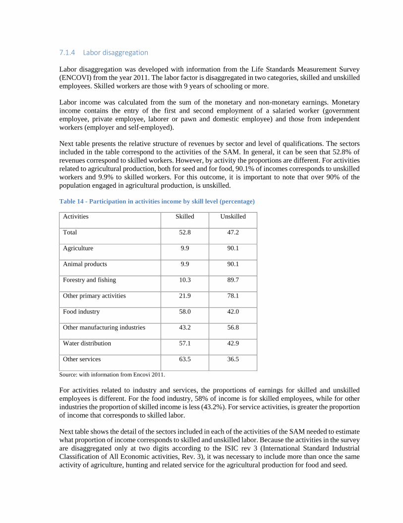
7.1.4 Labor disaggregation

Labor disaggregation was developed with information from the Life Standards Measurement Survey(ENCOVI) from the year 2011. The labor factor is disaggregated in two categories, skilled and unskilledemployees. Skilled workers are those with 9 years of schooling or more.

Labor income was calculated from the sum of the monetary and non-monetary earnings. Monetaryincome contains the entry of the first and second employment of a salaried worker (governmentemployee, private employee, laborer or pawn and domestic employee) and those from independentworkers (employer and self-employed).

Next table presents the relative structure of revenues by sector and level of qualifications. The sectorsincluded in the table correspond to the activities of the SAM. In general, it can be seen that 52.8% ofrevenues correspond to skilled workers. However, by activity the proportions are different. For activitiesrelated to agricultural production, both for seed and for food, 90.1% of incomes corresponds to unskilledworkers and 9.9% to skilled workers. For this outcome, it is important to note that over 90% of thepopulation engaged in agricultural production, is unskilled.

Table 14 - Participation in activities income by skill level (percentage)

Activities Skilled Unskilled

Total 52.8 47.2

Agriculture 9.9 90.1

Animal products 9.9 90.1

Forestry and fishing 10.3 89.7

Other primary activities 21.9 78.1

Food industry 58.0 42.0

Other manufacturing industries 43.2 56.8

Water distribution 57.1 42.9

Other services 63.5 36.5

Source: with information from Encovi 2011.

For activities related to industry and services, the proportions of earnings for skilled and unskilledemployees is different. For the food industry, 58% of income is for skilled employees, while for otherindustries the proportion of skilled income is less (43.2%). For service activities, is greater the proportionof income that corresponds to skilled labor.

Next table shows the detail of the sectors included in each of the activities of the SAM needed to estimatewhat proportion of income corresponds to skilled and unskilled labor. Because the activities in the surveyare disaggregated only at two digits according to the ISIC rev 3 (International Standard IndustrialClassification of All Economic activities, Rev. 3), it was necessary to include more than once the sameactivity of agriculture, hunting and related service for the agricultural production for food and seed.

Table 15 - Activities of the SAM according to the activities included in the surveyActivities Activities in the survey according to the ISIC rev 3.

AgricultureAgriculture, hunting and related service activities

Grow Coffee

Animal production

Agriculture, hunting and related service activities

Grow Coffee

Fishing, operation of fish hatcheries and fish farms; serviceactivities incidental to fishing

Forestry and fishing

Agriculture, hunting and related service activities

Forestry, logging and related service activities

Grow Coffee

Other primary activities Mining and quarrying

Food industry Manufacture of food products and beverages

Other manufacturing industries Rest of manufacturing

Water distribution Collection, purification and distribution of water

Other services Rest of services

Source: with information from Encovi 2011 and ISIC rev 3.

7.1.5 Household disaggregation

For this exercise we disaggregated into four representative household groups, by poverty level and byurban/rural areas. Households that do not reach to cover the minimum cost necessary to meet the foodand non-food needs are considered poor households, according to the official estimation of poverty forGuatemala. For the definition of urban areas, the survey uses the same of the latest census of populationand housing of 2002. The table below shows the proportion of each group of household.

Table 16 - Share of each group of household (percentage)

Household group Percentage

Urban poor 16.6

Rural poor 36.5

Urban non-poor 31.8

Rural non-poor 15.0

Source: with information from Encovi 2011.

Household income

For each representative household group, income is disaggregated according to the source of income andthe expenditure for each commodity. For all income components, the annual value is obtained bymultiplying by 12 the income received on a monthly basis, and by four income received during the lastthree months. As already mentioned, the labor income includes labor income by skilled and unskilledworker. Skilled workers are those aged 15 or more, with 9 years of schooling or more.

Capital income include rental income of rooms, housing, machinery, land, etc., interest and stockdividends. It does not include imputed rent. Government transfers to households, include income frombenefits welfare programs23, the income on account of retirement or pension and the money received forscholarships and/or school transport subsidy.

The money received from remittances from people living abroad are the transfers received from the restof the world. The income from the land was estimated from the sale or lease of land for agricultural usein the past twelve months. The following table shows the survey variables corresponding to each type ofincome.

Next table shows the relative structure of income, according to the source of income, for each householdgroup. It can be seen that the largest share of skilled labor income corresponds to non-poor urbanhouseholds, just as capital incomes. Importantly, government transfers are aimed primarily at non-poorurban households, because pensions and retirement income are included. Transfers from the rest of theworld are mainly aimed to the non-poor, urban and rural households. The land income, corresponds mostto the non-poor rural households.

Table 17 - Share of income for each household group

Percentage

Source of income Urban poor Rural poorUrban non-

poorRural non-poor

Labor income 9.9 14.1 61.5 14.4

Skilled 4.9 2.7 83.4 9.0

Non-skilled 15.6 26.9 36.9 20.6

Capital income 3.4 0.2 95.3 1.2

Government transfers 9.3 24.8 54.3 11.6

Transfers from the rest of the world 6.5 16.5 47.8 29.2

Land income 21.4 20.1 18.2 40.4

Source: with information of Encovi 2011.

23 The benefits of social assistance programs include the estimation of how much people would pay if they had to buy the benefitprovided by an institution of the Government.

Household expenditure

Household expenditure on goods and services include the spending on food, spending on goods andservices performed last week, last month and the last 12 months. Spending on energy sources used bythe household and media. Also it’s included the spending on transport and household services. Detailedexpenditure on goods and services by household group is included in next table. It can be seen that ingeneral the consumption of urban non-poor households is greater in most goods and services. Theconsumption of poor rural households is higher in some specific products such as corn, forestry and somebaked goods. The consumption of urban poor households is low in most products, in part because theyrepresent a smaller proportion, as well as non-poor rural households.

Table 18 - Household expenditure in good and services according to household groups (percentage)

No. CommoditiesUrbanpoor

Ruralpoor

Urbannon-poor

Rural non-poor

Total 10.0 19.2 52.3 18.4

1 Bananas 10.5 21.4 49.4 18.7

2 Coffee 13.4 26.3 42.8 17.5

3 Maize 14.9 50.5 13.1 21.6

4 Beans 14.4 35.3 31.4 18.9

5 Cereals and legumes 13.4 25.8 41.8 19.0

6 Roots and tubers 12.6 24.9 41.8 20.7

7 Vegetables 11.5 22.3 46.6 19.5

8 Fruits 9.0 15.2 57.2 18.6

9 Living plants 3.1 2.0 82.7 12.1

10 Other animal products 11.6 19.3 51.3 17.8

11 Firewood 16.2 45.4 16.1 22.3

12 Fish and fishery products 6.6 16.5 53.6 23.3

13 Other minerals 11.7 23.8 47.2 17.3

14 Meat and meat products 11.2 17.6 52.7 18.6

15 Prepared or preserved fish 6.3 13.4 59.6 20.6

16Prepared and preservedvegetables, legumes, etc.

6.7 10.6 61.9 20.7

17Animals and vegetables oilsand fats

12.4 22.5 45.9 19.2

18 Grain mill products 11.3 31.5 35.1 22.0

19Preparation used in animalfeeding

4.8 20.8 52.4 21.9

20 Bakery products 13.9 32.1 35.0 19.1

21 Sugar 14.2 32.8 33.7 19.3

22Noodles and similarfarinaceous products

13.3 25.1 42.3 19.2

23 Dairy products 8.5 10.0 64.2 17.4

24 Food products n.e.c. 10.4 16.5 53.4 19.7

25Alcoholic and non-alcoholicbeverage

7.9 12.3 61.9 17.9

26 Other industries 8.2 12.6 60.5 18.7

27 Water and electricity 10.5 12.2 61.9 15.5

28 Lodging 3.4 4.6 75.3 16.7

29 Other services 6.5 6.9 71.0 15.6Source: with information from Encovi 2011.

7.2 Guatemala's economic structure tables

Table 19 - Consumption composition of each household group (percentage)

Urbanpoor

Ruralpoor

Urban non-poor

Rural non-poor

Coffee 0.0 0.0 0.0 0.0

Bananas 1.4 1.5 0.6 0.8

Maize 4.3 4.7 2.6 3.3

Beans 3.8 6.8 0.4 2.4

Cereal and legumes 0.2 0.3 0.1 0.1

Roots and tubers 2.4 2.5 1.0 1.5

Vegetables 7.0 7.4 3.0 4.9

Fruits 1.7 1.7 0.9 1.2

Living plants 0.2 0.2 0.2 0.2

Milk 0.1 0.0 0.3 0.1

Eggs 1.1 0.6 1.3 1.0

Other animal products 0.0 0.0 0.0 0.0

Firewood 1.3 1.2 0.8 0.9

Other forestry and logging products 1.6 2.3 0.2 0.9

Fish and fishery products 0.5 0.7 0.1 0.3

Other minerals 0.1 0.1 0.1 0.1

Meat and meat products 6.0 6.5 3.2 3.8

Prepared or preserved fish 0.3 0.3 0.2 0.2

Prepared and preserved vegetables 0.4 0.5 0.5 0.6

Animal and vegetable oils and fats 0.8 0.7 1.0 1.1

Grain mill products 5.3 5.1 2.5 3.5

Preparation used in animal feeding 0.2 0.3 0.1 0.2

Bakery products 4.8 11.1 6.8 9.4

Sugar 3.1 3.8 1.0 1.8Noodles and similar farinaceousproducts

0.8 1.0 0.3 0.5

Dairy products 4.0 4.0 1.7 2.5

Food products n.e.c. 2.4 1.5 2.4 2.2

Alcoholic and non-alcoholic beverages 1.5 1.2 1.0 1.2

Other industries 22.5 18.7 23.0 21.9

Water and electricity 1.0 0.8 1.0 1.0

Lodging 8.4 5.2 6.5 5.3

Other services 12.8 9.3 37.3 27.3

Total 100.0 100.0 100.0 100.0Source: Social Accounting Matrix for Guatemala, 2011.

7.3 Sensitivity results

If we change elasticities of production, consumption, CET, Trade, we observe that our model has moresensibility to elasticity of production, especially for agriculture, forestry and fishing, and other primaryactivites. In any case the sign of the effect changed from negative to positive.

Figure 4 - Sensitivity results

Source: own calculations based on PEP 1-1 Model

(30.0) (20.0) (10.0)

- 10.0 20.0 30.0 40.0 50.0

Climate Change

Elasticity Production CETConsumption TradeBase

(20.0) (15.0) (10.0)

(5.0) -

5.0 10.0 15.0 20.0 25.0 30.0

Drought

Elasticity Production CETConsumption TradeBase