final report for air force research laboratory aerospace ... · air force research laboratory...
TRANSCRIPT

Final Report
for
Air Force Research Laboratory Aerospace Systems Directorate
Design Optimization of
Slotted Waveguide Antenna Stiffened Structures
Date: 8 January 2014
Desired Initial Funding Period: 1 Jan 2011–31 Dec 2013
Proposed Duration of Project: 36 Months
Principal Investigator: Robert A. Canfield
Aerospace and Ocean Engineering Department
Virginia Polytechnic Institute and State University
214 Randolph Hall
Blacksburg, VA 24061
(540) 231-5981

REPORT DOCUMENTATION PAGE Form Approved
OMB No. 0704-0188 Public reporting burden for this collection of information is estimated to average 1 hour per response, including the time for reviewing instructions, searching existing data sources, gathering and maintaining the data needed, and completing and reviewing this collection of information. Send comments regarding this burden estimate or any other aspect of this collection of information, including suggestions for reducing this burden to Department of Defense, Washington Headquarters Services, Directorate for Information Operations and Reports (0704-0188), 1215 Jefferson Davis Highway, Suite 1204, Arlington, VA 22202-4302. Respondents should be aware that notwithstanding any other provision of law, no person shall be subject to any penalty for failing to comply with a collection of information if it does not display a currently valid OMB control number. PLEASE DO NOT RETURN YOUR FORM TO THE ABOVE ADDRESS.
1. REPORT DATE (DD-MM-YYYY)
08-01-2014 2. REPORT TYPE
Final Technical Report
3. DATES COVERED (From - To)
1 Jan 2011–31 Dec 2013
4. TITLE AND SUBTITLE 5a. CONTRACT NUMBER
FA8650-09-2-3938
Title: AFRL-VT-WSU Collaborative Center on Multidisciplinary
Sciences
5b. GRANT NUMBER
Subtitle: Design Optimization of Slotted Waveguide Antenna
Stiffened Structures (SWASS)
5c. PROGRAM ELEMENT NUMBER
6. AUTHOR(S) 5d. PROJECT NUMBER
Kim, Woon Kyung, Postdoc, Virginia Tech 5e. TASK NUMBER
Canfield, Robert A., Professor, Virginia Tech 5f. WORK UNIT NUMBER
7. PERFORMING ORGANIZATION NAME(S) AND ADDRESS(ES)
AND ADDRESS(ES)
8. PERFORMING ORGANIZATION REPORTNUMBER
Aerospace and Ocean Engineering (MC0203)
Randolph Hall, RM 215, Virginia Tech VT-AOE-13-002
9. SPONSORING / MONITORING AGENCY NAME(S) AND ADDRESS(ES) 10. SPONSOR/MONITOR’S ACRONYM(S)
William Baron, and James Tuss
Aerospace Systems Directorate, AFRL, WPAFB,OH 11. SPONSOR/MONITOR’S REPORT
NUMBER(S)
12. DISTRIBUTION / AVAILABILITY STATEMENT
APPROVED FOR PUBLIC RELEASE; DISTRIBUTION UNLIMITED.
13. SUPPLEMENTARY NOTES
14. ABSTRACT
The objective of the research is to investigate computational methods for design optimization of a
Conformal Load-Bearing Antenna Structure (CLAS) concept. Research centers on investigating
computational methods for design optimization of a slotted waveguide antenna stiffened structure
(SWASS). The goal of this concept is to turn the skin of aircraft into a radio frequency (RF) antenna.
SWASS is a multidisciplinary blending of RF slotted waveguide technology and stiffened composite
structures technology. Waveguides provide channels for RF signal transmission, as well as structural
stiffening. A SWASS skin or stiffener will have numerous slots that allow the RF energy to radiate to
the atmosphere. Slot design for maximum RF performance with minimum structural performance degradation
due to the slots will be the multidisciplinary, multiobjective design challenge. Initially, waveguides
acting as hat stiffeners were considered in this research; then, waveguides that constituted the core
of a sandwich panel were designed for loads in the aircraft skin. The concept design requires
parameterization of slot shape, size, location, and spacing in conjunction with stiffener or core
sizing and spacing, composite material selection, and laminate layout in order to simultaneously meet
desired structural and RF performance. 15. SUBJECT TERMS
SWASS, CLAS, slotted waveguide, response surface methodology, multifunctional composite
structure, SORCER
16. SECURITY CLASSIFICATION OF: 17. LIMITATIONOF ABSTRACT
18. NUMBEROF PAGES
19a. NAME OF RESPONSIBLE PERSON
Robert A. Canfield
a. REPORT
U
b. ABSTRACT
U
c. THIS PAGE
U UU 69
19b. TELEPHONE NUMBER (include area
code)
540-231-5981
Standard Form 298 (Rev. 8-98) Prescribed by ANSI Std. Z39.18

iii
Executive Summary
Title: Design Optimization of Slotted Waveguide Antenna Stiffened Structures (SWASS)
Principal Investigator: Dr. Robert A. Canfield
Research Objectives:
Verify multi-fidelity models of SWASS waveguide tubes for both electromagnetic (EM)
and structural performance. Validate structural finite element model (FEM) against
experimental results.
Quantify the tradeoff between structural and RF performance for characteristic integrated
SWASS design concepts. Formulate multidisciplinary analysis and design optimization
problem for SWASS using finite element meshes based on common geometry.
Deliver computational models and source for SWASS design optimization that is
compatible and functions with Service ORiented Computing EnviRonment (SORCER).
Synopsis of Research: The objective of the research is to investigate computational methods
for design optimization of a Conformal Load-Bearing Antenna Structure (CLAS) concept.
Research centers on investigating computational methods for design optimization of a slotted
waveguide antenna stiffened structure (SWASS). The goal of this concept is to turn the skin of
aircraft into a radio frequency (RF) antenna. SWASS is a multidisciplinary blending of RF
slotted waveguide technology and stiffened composite structures technology. Waveguides
provide channels for RF signal transmission, as well as structural stiffening. A SWASS skin or
stiffener will have numerous slots that allow the RF energy to radiate to the atmosphere. Slot
design for maximum RF performance with minimum structural performance degradation due to
the slots will be the multidisciplinary, multiobjective design challenge. Initially, waveguides
acting as hat stiffeners were considered in this research; then, waveguides that constituted the
core of a sandwich panel were designed for loads in the aircraft skin. The concept design
requires parameterization of slot shape, size, location, and spacing in conjunction with stiffener
or core sizing and spacing, composite material selection, and laminate layout in order to
simultaneously meet desired structural and RF performance.

iv
Table of Contents Executive Summary ............................................................................................................... iii
List of Figures ......................................................................................................................... vi
List of Tables ........................................................................................................................ viii
Chapter 1 Introduction ........................................................................................................... 1
1.1 Objectives ................................................................................................................. 1
1.2 Air Force Relevance ................................................................................................. 1
1.3 Background ............................................................................................................... 1
1.3.1 Structurally Integrated Antennas on a Joined-Wing Aircraft ............................ 2
1.3.2 Aircraft X-Band Radar ...................................................................................... 3
1.3.3 Electromagnetic Performance for Waveguides ................................................. 3
1.3.4 Structural Analysis and Design ......................................................................... 4
1.3.5 Software for Antenna Design ............................................................................ 7
1.4 Problem Definition and Scope .................................................................................. 8
1.5 Summary of Research ............................................................................................... 9
1.6 Deliverables .............................................................................................................. 9
1.7 Technical Team Members......................................................................................... 9
Chapter 2 Radio Frequency Optimization of Slotted Waveguide Antenna Stiffened
Structure 11
2.1 Introduction ............................................................................................................. 11
2.2 RF Analysis of WR-90 Slotted Waveguide Antenna ............................................. 12
2.2.1 Computational Modeling for Radiation ........................................................... 12
2.2.2 Sensitivity results for WR-90 waveguide ........................................................ 14
2.3 Optimization ........................................................................................................... 18
2.3.1 Problem Statement ........................................................................................... 18
2.3.2 Gradient-Based Optimization .......................................................................... 18
2.3.3 Response Surface Methodology ...................................................................... 21
2.4 Conclusions and Future Work ................................................................................ 24
Chapter 3 Structural Design and Optimization of Slotted Waveguide Antenna Stiffened
Structures Under Compression Load ............................................................................................ 25
3.1 Introduction ............................................................................................................. 25
3.2 Design Concepts of SWASS ................................................................................... 26
3.3 Equivalent 2D modeling ......................................................................................... 28
3.3.1 Equivalent modeling of core webs .................................................................. 28
3.3.2 Mathematical formation .................................................................................. 28

v
3.3.3 Model verification ........................................................................................... 30
3.4 3D FEM Plate Model .............................................................................................. 32
3.4.1 Model verification of 3D plate FEM model .................................................... 32
3.4.2 Structural instability of four design concepts of SWASS ............................... 33
3.5 Structural Analysis and Evaluation ......................................................................... 35
3.5.1 Nonlinear analysis ........................................................................................... 35
3.5.2 Structural optimization .................................................................................... 37
3.5.3 Experimental results ........................................................................................ 38
3.6 Conclusions and Future Work ................................................................................ 41
Chapter 4 Distributed Computation for Design Optimization of Aircraft ........................... 42
4.1 Introduction ............................................................................................................. 42
4.2 Project Description.................................................................................................. 42
4.3 Background Work ................................................................................................... 43
4.4 Implementation in SORCER Environment ............................................................. 44
4.4.1 Example of nonlinear aeroelastic scaling model ............................................. 44
4.4.2 Example of SWASS structural model ............................................................. 45
4.5 Current Issues and Future Work ............................................................................. 46
4.6 Conclusion .............................................................................................................. 47
4.7 Tutorial Links.......................................................................................................... 47
Chapter 5 Conclusions and Recommendations.................................................................... 48
Acknowledgement .................................................................................................................. 49
List of References .................................................................................................................. 50
Appendix A. Electromagnetic Part ....................................................................................... 53
A.1 Electromagnetic Convergence Study ....................................................................... 53
Appendix B. Structural Part ................................................................................................. 56
B.1 Buckling Analysis of Non-slotted and Slotted Waveguide Tubes .......................... 56
B.2 Interlaminar Shear Stresses ...................................................................................... 58
vi
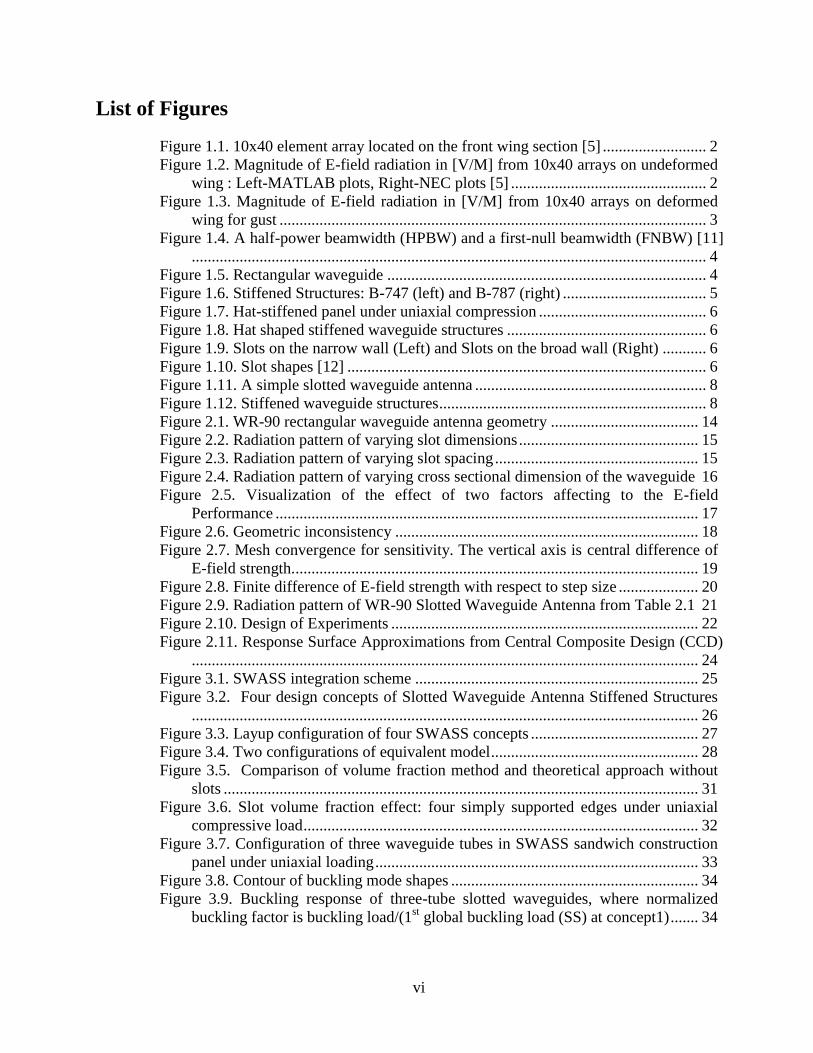
List of Figures
Figure 1.1. 10x40 element array located on the front wing section [5] .......................... 2 Figure 1.2. Magnitude of E-field radiation in [V/M] from 10x40 arrays on undeformed
wing : Left-MATLAB plots, Right-NEC plots [5] ................................................. 2 Figure 1.3. Magnitude of E-field radiation in [V/M] from 10x40 arrays on deformed
wing for gust ........................................................................................................... 3
Figure 1.4. A half-power beamwidth (HPBW) and a first-null beamwidth (FNBW) [11]
................................................................................................................................. 4 Figure 1.5. Rectangular waveguide ................................................................................ 4 Figure 1.6. Stiffened Structures: B-747 (left) and B-787 (right) .................................... 5 Figure 1.7. Hat-stiffened panel under uniaxial compression .......................................... 6
Figure 1.8. Hat shaped stiffened waveguide structures .................................................. 6 Figure 1.9. Slots on the narrow wall (Left) and Slots on the broad wall (Right) ........... 6
Figure 1.10. Slot shapes [12] .......................................................................................... 6 Figure 1.11. A simple slotted waveguide antenna .......................................................... 8 Figure 1.12. Stiffened waveguide structures ................................................................... 8 Figure 2.1. WR-90 rectangular waveguide antenna geometry ..................................... 14 Figure 2.2. Radiation pattern of varying slot dimensions ............................................. 15 Figure 2.3. Radiation pattern of varying slot spacing ................................................... 15 Figure 2.4. Radiation pattern of varying cross sectional dimension of the waveguide 16
Figure 2.5. Visualization of the effect of two factors affecting to the E-field
Performance .......................................................................................................... 17
Figure 2.6. Geometric inconsistency ............................................................................ 18 Figure 2.7. Mesh convergence for sensitivity. The vertical axis is central difference of
E-field strength...................................................................................................... 19 Figure 2.8. Finite difference of E-field strength with respect to step size .................... 20
Figure 2.9. Radiation pattern of WR-90 Slotted Waveguide Antenna from Table 2.1 21 Figure 2.10. Design of Experiments ............................................................................. 22 Figure 2.11. Response Surface Approximations from Central Composite Design (CCD)
............................................................................................................................... 24
Figure 3.1. SWASS integration scheme ....................................................................... 25 Figure 3.2. Four design concepts of Slotted Waveguide Antenna Stiffened Structures
............................................................................................................................... 26 Figure 3.3. Layup configuration of four SWASS concepts .......................................... 27 Figure 3.4. Two configurations of equivalent model .................................................... 28
Figure 3.5. Comparison of volume fraction method and theoretical approach without
slots ....................................................................................................................... 31
Figure 3.6. Slot volume fraction effect: four simply supported edges under uniaxial
compressive load ................................................................................................... 32 Figure 3.7. Configuration of three waveguide tubes in SWASS sandwich construction
panel under uniaxial loading ................................................................................. 33 Figure 3.8. Contour of buckling mode shapes .............................................................. 34
Figure 3.9. Buckling response of three-tube slotted waveguides, where normalized
buckling factor is buckling load/(1st global buckling load (SS) at concept1) ....... 34

vii
Figure 3.10. Weight-normalized buckling of three-tube slotted waveguides, where
Normalized BF = Buckling load/(1st global buckling load (SS) at concept1), and
Normalized Weight = Weight at each concept/(Weight at concept1). ................. 35 Figure 3.11. Two different boundary conditions: contours on top and bottom face sheet
strains in fiber direction (concept 1). Unit: in/in ................................................... 36 Figure 3.12. Fiber direction strain under compressive loading in the initial design. The
applied design load (12000 lbf (53.4kN)) is determined by the circular pink-dotted
line of Concept 4 (1000 lbf = 4.45kN) .................................................................. 36 Figure 3.13. Mass efficiency for four different SWASS design concepts before and
after optimization .................................................................................................. 38 Figure 3.14. Post-optimization curves. ......................................................................... 38 Figure 3.15. MTS compressive load test (ASTM C364) .............................................. 39 Figure 3.16. Comparison of fiber direction strains: 5ply E-glass on both sides (1000 lbf
= 4.45kN) .............................................................................................................. 40 Figure 3.17. Comparison of fiber direction strains: 5ply E-glass on both sides (1000 lbf
= 4.45kN) .............................................................................................................. 41 Figure 4.1. Flowchart of Equivalent Static Loads optimization [45] provided by
Anthony Ricciardi. ................................................................................................ 43 Figure 4.2. Flowchart of Ricciardi’s Nonlinear Aeroelastic Scaling procedure within
the SORCER environment .................................................................................... 45
Figure 4.3. Example of SWASS structural response using the SORCER, demonstrating
the buckling of Concept 1 ..................................................................................... 46
Figure B. 1. Comparison of non-slotted and slotted waveguide tubes. ........................ 56 Figure B. 2. Buckling modes of non-slotted and slotted waveguide tubes. .................. 57 Figure B. 3. Concept 1: Interlaminar shear stress curves. The post-optimization curves
satisfy the interlaminar shear stress requirements at the design load of 12,000 lbf
(see Chapter 3). ..................................................................................................... 58 Figure B. 4. Concept 2: Interlaminar shear stress curves. ............................................ 59 Figure B. 5. Concept 3: Interlaminar shear stress curves. ............................................ 60
Figure B. 6. Concept 4: Interlaminar shear stress curves. ............................................ 61

viii
List of Tables
Table 2.1. Optimal Design Values ................................................................................ 20 Table 2.2. Electric field peak magnitude using RSM ................................................... 23 Table 3.1. Material properties [41] ............................................................................... 31 Table 3.2. Comparison of structural instability between Sabat's and 3D plate models 32
Table 3.3. SWASS compression test panel ................................................................... 39
Table A. 1 Convergence of meshes .............................................................................. 53 Table A. 2. Rectangular waveguide standards .............................................................. 55

1
Chapter 1 Introduction
1.1 Objectives Existing antennas are attached to an aircraft surface as blades or enclosed within the aircraft
structure, typically covered by electromagnetically transparent and structurally weak composite
materials such as fiberglass. In contrast, conformal antennas may be integrated into the
honeycomb core, stiffeners or the skin of aircraft surface panels. In the case of a waveguide
structure, the size can be bigger than antennas that are located on the surface of the fuselage.
Therefore, it can bear more internal or external forces than other antenna structures. Since this
new concept antenna structure can be installed in the main part of load bearing structures, it will
perform the roles of a structure and an antenna. The goal is to use Multidisciplinary Design
Optimization (MDO) to achieve high structural performance, such as the strength or stiffness,
and simultaneously maintain antenna characteristics, such as the gain or beam pattern. Ultimately,
the research objective is to quantify the synergistic benefit of simultaneous structural and RF
design of SWASS.
1.2 Air Force Relevance Airframe structures have been developed historically from a fabric covered wood, later from
aluminum skin and stringer frame, and now more frequently from high modulus composite [1].
Most Radio Frequency (RF) engineers are interested in designing antennas and radomes
independently, and then they try to resolve the interface problems. However, the opportunity
exists to pursue a novel technology to structurally integrate antennas.
The most common benefit of the structurally integrated antenna is drag reduction [2]. Large
antenna structures, such as reflecting dishes or planar arrays that cause drag, are mounted in
fairings or radomes of existing aircraft. An opportunity exists for structurally integrated antennas
to replace many protruding antennas. In addition, removing external antennas can reduce radar
cross section (RCS) of an aircraft. There are many other merits besides reducing the RCS of an
aircraft. External antennas such as blades can be damaged, when objects pass close to the aircraft
outer mold line (OML) [2] and contact the antennas. They are subject to impact in flight
operation, ground handling, and maintenance. Specifically, fixed wing aircraft might fly through
inclement weather such as hailstorm or gust, and rotorcraft might contact foliage or objects when
operating from a harsh helipad. Moreover, an aircraft can obtain more lift force by adopting
structurally embedded antennas [2]. Since the antenna is usually bulky, if it is incorporated into
other components, good aerodynamic performance can be achieved.
1.3 Background A few programs such as Conformal Load-Bearing Antenna Structure (CLAS) [2], Smart Skin
Structures Technology Demonstration (S3TD) [3], and RF Multifunction Structural Aperture
(MUSTRAP) [4] strove to advance the technology of integrating structures and antennas to
produce higher efficiency of the design and maintenance. Significant contributions of these
programs are a weight saving and drag reduction. At the Air Force Institute of Technology
(AFIT) Smallwood, Canfield and Terzoulli studied a structurally integrated antenna mounted
into the wings of a joined-wing aircraft [5]. Recently, high frequency microstrip antennas
embedded in aircraft skin were examined [6]. The microstrip patch antenna was installed to a
space between a facesheet and a honeycomb structure.

2
1.3.1 Structurally Integrated Antennas on a Joined-Wing Aircraft
The AFIT research sought to study a concept that embeds conformal load-bearing antenna
arrays into the wing structure of a joined-wing aircraft [5]. Because the wings deform under the
flight condition, it could affect the original configuration of the antenna. Therefore, the effect in
antenna performance was measured against wing deformation. Smallwood et al [5] used half-
wavelength dipoles to model the conformal load-bearing antenna element and a commercial
software package, NEC-Win Plus+TM
using the Method of Moments solution technique, to prove
the analytic model. A simple model of the sensors was generated to integrate the different layers
of materials to construct antenna’s structure. A simplified finite element model of antenna
consisted of five layers, which were an electromagnetically transparent material called
Astroquartz, two honeycomb core structures, and two graphite epoxy layers. Astroquartz and
graphite epoxy are modeled as symmetric composite layers with 0o, +/-45
o, and 90
o plies. Wing
deformations were generated on a fully stressed design by an integrated software environment
using the Adaptive Modeling Language (AML), MSC.NASTRAN, and PanAir. These
deformations were used to locate the new position and slope of each element of array. Then, a
new beam pattern was generated. They repeated this process for the various load configurations.
Baseline results and repeated process results were compared to determine the beam pointing
error due to the wing deformations.
NEC-Win Plus+TM
and dipole theory implemented in MATLAB were used to produce
radiation patterns on the undeformed and deformed wing. The radiation pattern of 10x40 element
array located close to the fuselage, depicted in Figure 1.1, was calculated for the undeformed and
deformed wing under the gust load. Results from each method were compared in Figure 1.2 and
Figure 1.3. The overall patterns showed some similarities, but the array theory patterns were
wider than the NEC patterns. For a deformed wing due to a steady 2.5g maneuver load and a gust
load, the radiation pattern was affected by the deformation, but the azimuth angles were
essentially the same. The worst pointing error of approximately 9o occurred for a gust load
condition.
Figure 1.1. 10x40 element array located on the front wing section [5]
Figure 1.2. Magnitude of E-field radiation in [V/M] from 10x40 arrays on undeformed
wing : Left-MATLAB plots, Right-NEC plots [5]

3
Figure 1.3. Magnitude of E-field radiation in [V/M] from 10x40 arrays on deformed wing
for gust
1.3.2 Aircraft X-Band Radar
Every aircraft has an electronic device for radio detecting and ranging (radar). Radar radiates
electromagnetic waves to detect far off objects such as aircraft, ships, and buildings, and
recognize them by the reflecting echo from the objects. In other words, aircraft radar can be
compared to a major visual center of a pilot in the sky. In addition, radar is not only used for
satellite communication but also to control military weapons [7].
The microwave band was divided into narrow bands and allocated letters for purpose of
military security: L, S, C, X, and K-band. Compared to the higher frequencies, the hardware is
larger for the lower frequencies, since the wavelengths are long. Higher frequencies have a
higher limitation on the power transmission. Nevertheless, microwave devices have some merits.
Firstly, they can focus a narrow beam to detect targets accurately. The power can be accordingly
concentrated in a particular direction. Secondly, microwaves pass through the atmosphere with
low attenuation of absorption and scattering due to water vapors or raindrops. Below about 0.1
GHz, the atmospheric attenuation such as absorption and scattering is negligible, but it becomes
significant beyond 10 GHz. Lastly, ambient noise is gradually decreased from L-band to X-Band,
but it become increasingly higher than K-band [8]. For those reasons, X-band radar systems of 8
to 12.5 GHz are usually used for fighter aircraft. For example, F-14, F-15, F-16, and F/A-18 use
X-band radar systems such as AN/APG-63, 65, 68, 70, 71 and 73 [9].
Waveguide components may replace lumped circuit elements in the frequency from 1 to 100
GHz. Because radar typically uses microwave frequencies, waveguide antennas are good
airborne radar antennas for satellite communication, detecting targets, and missile-tracking or
guidance radar [10]. The waveguide antenna frequency of this research will be focused at 10
GHz frequency in the X-band.
1.3.3 Electromagnetic Performance for Waveguides
The gain is defined as
( , )4
in
UG
P
(1.1)
where Pin is the total input power and ( , )U is the radiation intensity [11]. Beamwidth is the
configuration of the mainlobe. There are two types of beamwidth characterization. One is the
half-power beamwidth (HPBW) and another one is first-null beamwidth (FNBW), shown in

4
Figure 1.4 [11]. Those are determined by the slotted waveguide design. The slot shape and
dimension yield the desired radiation pattern. The antenna size determines the frequency of the
radiation. In addition, the frequency depends on the cross sectional shape and dimension of the
waveguide antenna [12]. The frequency is determined as
f
c
(1.2)
where f is the frequency, λ is the wavelength, and c is the speed of light. Also, cut-off frequency,
which is the minimum frequency to propagate waves, is
2 2
2c
c m nf
a b
(1.3)
in which a is the width of the rectangular waveguide, b is the height of the rectangular
waveguide shown in Figure 1.5, ε is the dielectric constant, μ is the magnetic permeability within
the waveguide, m and n are the numbers of the mode variations for transverse electric (TE) or
transverse magnetic (TM) waves [13].
Figure 1.4. A half-power beamwidth (HPBW) and a first-null beamwidth (FNBW) [11]
Figure 1.5. Rectangular waveguide
1.3.4 Structural Analysis and Design
In the case of the structures, optimum designs must consider local and global buckling,
ultimate strength of tension and compression, strain, and so on [14]. The stability of structures
such as local buckling will be considered, since stiffeners, such as those shown in Figure 1.6,

5
may reach the local buckling load prior to the ultimate strength. When panel buckling occurs, it
may affect the electromagnetic waves due to the variation of the waveguide antenna section. The
critical stress of panel buckling, x cr , with four edges of a rectangular plate simply supported
under uniaxial loads is
2 2 22
2 2( ) ( )x cr
s
D n am
t a m b
(1.4)
in which D is the flexural rigidity of an isotropic flat plate, 3
212(1 )
s s
s
E t
, Es is the modulus of
elasticity of the face sheet material, νs is the Poisson ratio of face sheet material, ts is the
thickness of face sheet, a is the length of global panel, b is the width of rectangular flat plate
segment, m is the number of the buckle half-sine waves in x-direction, and n is the number of the
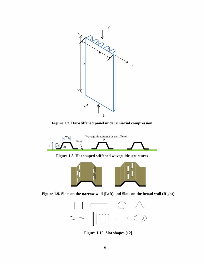
buckle half-sine wave in y-direction, shown in Figure 1.7 [14]. Accordingly, the width of flange,
the height of web, and the angle between the web and flange, shown in Figure 1.8, may be the
design variables to optimize the hat-stiffened antenna structures. The waveguide slots might be
placed on the broad wall surface or the side surface of the hat stiffeners in Figure 1.9. Slot shapes,
shown in Figure 1.10, would be designed to make the intended radiation pattern [12].
The specific strength and specific modulus will be compared to conventional stiffeners. The
specific strength is the ratio between the strength and the weight and the specific stiffness is the
ration between the stiffness and the weight. The specific strength and specific modulus is
Specific strength=
(1.5)
Specific modulus=
E
(1.6)
in which σ is the strength, ρ is the density, and E is the modulus of elasticity of the material.
Figure 1.6. Stiffened Structures: B-747 (left) and B-787 (right)
6
Figure 1.7. Hat-stiffened panel under uniaxial compression
Figure 1.8. Hat shaped stiffened waveguide structures
Figure 1.9. Slots on the narrow wall (Left) and Slots on the broad wall (Right)
Figure 1.10. Slot shapes [12]
a y
x
P
P
b

7
1.3.5 Software for Antenna Design
Techniques are classified as to whether they are solved in the time or frequency domain.
Another classification is partial differential equation (PDE) or integral equation to solve the
differential or integral form of Maxwell's equations. For example, Method of Moments (MoM)
employs frequency domain and integral techniques; on the other hand FEM solves the
discretized PDE’s. Finite Difference Time Domain (FDTD) obviously uses is the time domain
approach. Though MoM and FEM need a matrix solver to get solutions, FDTD does not require
a matrix solver [15], because FDTD employs an explicit method.
The COMSOL Multiphysics FEM software simulates the physics with PDEs. It provides a
number of predefined modeling interfaces for applications from fluid flow and heat transfer to
structural mechanics and electromagnetic analysis. Specific modules contribute material libraries,
solvers and elements. There are some modules to provide specific interfaces, includingand RF
Module and Structural Mechanics Module. The RF module is based on Maxwell’s equations of
electromagnetic fields and waves, considered in Chapter 2. It provides advanced postprocessing
features such as a far-field analysis. Application examples are antennas, waveguides and cavities,
S-parameter analyses of antennas, and transmission lines. The structural mechanics module
focuses on the structural deformation and stress analysis of components and subsystems and
works in tandem with COMSOL Multiphysics [16].
FEKO is an electromagnetic analysis software using Method of Moment (MoM) with hybrid
techniques employing FEM. Typical applications are antennas, antenna placement, RF
components, radomes and so on. It is used in many industries such as automotive, aerospace,
naval, RF components, antenna design, mobile phone, bio-electromagnetic, and even
communication. There are three major components CADFEKO, EDITFEKO, and POSTFEKO
about the FEKO user interface. CADFEKO is used to make geometry and do the required
meshing for the FEKO solution kernel. EDITFEKO helps the user for creating or editing the
input file. POSTFEKO is used for post processing purposes and visualizing the geometry of the
FEKO model [17].
CST MICROWAVE STUDIO (CST MWS) specializes in 3D EM simulation of high
frequency components such as antennas, filters, couplers and multi-layer structures. It provides
six powerful solver modules: transient solver, frequency domain solver, eigenmode solver,
resonant solver, integral equation solver and asymptotic solver. CST MWS uses a Finite
Integration Method (FIM) and time domain analysis. In the time domain, the numerical effort of
FIM increases more slowly with the problem size than other commonly employed methods [18].
HFSS is 3D full wave electromagnetic field simulation tool. It is one of the most well-known
and powerful applications used for antenna design and the design of complex RF electronic
circuit elements. It provides E-field and H-field, current, S-parameters, near and far field results.
HFSS automatically creates a mesh for solving the problem using FEM. HFSS provides
capability to analyze 3D radiating elements such as slot, horn, and patch antennas. It calculates,
directivity, impedance, and radiation patterns [19].
Among its user groups, CST MWS enjoys a reputation as user-friendly software [20]. It
provides both time domain and frequency domain analysis. In the case of FEKO, it can simulate
efficiently large antennas such as used on aircraft and naval ships. Having large user groups,
HFSS is perhaps the RF software best known over the world. COMSOL Multiphysics’ strong
point is that it can provide integrating solutions for multiple disciplines, such as electromagnetic
and structures. In contrast to HFSS, CST, and FEKO, COMSOL Multiphysics has both structural

8
and EM analysis. Based on this feature among the choices surveyed, COMSOL was chosen for
the initial SWASS design studies.
1.4 Problem Definition and Scope A typical slotted waveguide model is shown in Figure 1.11. In Chapter 2, we shall first
consider a multifunctional structure in which stiffeners act as slotted waveguides in Figure 1.12.
To optimize these components, the design parameters such as geometric dimensions are defined
in two categories. Firstly, one category is to optimize structures by minimizing weight, while
achieving sufficient stiffness and strength to bear loads. In a structural optimization, the design
variables are defined as the width, length, and thickness of waveguide antennas. The size of the
waveguide structures obviously determines structural weight. In stiffness, the antenna shape
influences the deformation of structures. The frequency of radiation determines the antenna size
and the significant dimension of the slot. Secondly, antenna objective functions are specified in
terms of desired gain, beamwidth of mainlobe or sidelobe, bandwidth, etc [13], governed by slot
dimensions (Figure 1.10). In Chapter 3 we shall next consider design of waveguide tubes (Figure
1.11) that comprise the core of the sandwich structure of aircraft panels (Figure 1.12). Factors
such as the dimension and location of waveguide slots are the EM design variables. To determine
the value of design variables that optimize these functions for an approximate system response, a
response surface method (RSM) [21] in ModelCenter was used in this research. Once derivatives
are available, then more efficient multipoint approximations may be used [22].
Figure 1.11. A simple slotted waveguide antenna
Figure 1.12. Stiffened waveguide structures
There are many materials for structures and antennas. Material properties affect the structural
characteristics such as stiffness or strength and the antenna characteristics such as a gain or a
beam pattern. In this research, composite materials are chosen for satisfying competing
requirements of the structures and antennas. In addition, stiffener beam shapes, thickness or sizes
are one of the important factors to support loads and radiate electronic waves. Therefore,

9
performance of the structures and antennas are varied by these factors. The factors can be used to
optimize structural and antenna performance. These research goals are to search for the optimal
structural and antenna design. To analyze the structure and antenna, a FEM is applied for both
structural analysis and antennas for electromagnetic field analysis. The decoupled analyses were
implemented in the SORCER [23, 24], as documented in Chapter 4, with a vision to eventually
implement the coupled design via SORCER.
1.5 Summary of Research Chapter 1 summarized a range of SWASS topic related to structural and electromagnetic
design concepts and design variables for optimal conditions. Next, Chapter 2 presents a
computational modeling methodology developed for design and optimization of slotted
waveguide antenna stiffened structure (SWASS). A FEM-based model technique was used to
configure a slotted waveguide array. Various geometric design variables were chosen for optimal
design approach, which enables one to impose stringent conditions on structural configurations.
Some of them are shown to have high impact on slot radiation pattern sensitivity. Sequential
quadratic program (SQP) and response surface methodology (RSM) were used with the FEM-
based modeling to quantify electromagnetic (EM) performance. Comparison of results from the
two optimizers confirmed the extent to approximate optimal designs using RSM for the SWASS
configuration which optimality conditions were satisfied
Chapter 3 addresses structural design and optimization of slotted waveguide antenna
stiffened structures (SWASS). Structural design and optimization will be performed by
designing the antenna structure imbedded aircraft panel subject to external loading, while
evaluating radio frequency (RF) performance. For complex composite structural analysis, firstly,
the equivalent model was proposed and compared to an analytical approach by simplifying 3D
structure into 2D plate model. For higher fidelity, 3D plate FEM models for these structures were
used to evaluate the mechanical failure and lightweight design criteria. This modeling technique
is highly cost-effective in that it has relatively small number of elements compared with 3D solid
modeling. This chapter demonstrated that it is sufficiently accurate compared to experiments and
other published simulations.
Chapter 4 focuses on the development of the SORCER for the synthesis of mutiobjective
function design and optimization through on-line database sharing. Structural analysis examples
are demonstrated.
1.6 Deliverables Various resources are saved at the websites “905123 Collaborative Center” and “SWASS”
at scholar.vt.edu. The final report provides design models and analysis incorporating all
journal/conference publications.
1.7 Technical Team Members Technical Team Leader: Robert A. Canfield (PI), Professor, Dept. of Aerospace and Ocean
Engineering Virginia Tech
Researchers: Woon Kim, Postdoctoral Research Associate,
Taekwang Ha, Graduate Student,
Garrett Hehn, Undergraduate Student,
Dept. of Aerospace and Ocean Engineering, Virginia Tech

10
Project Sponsor:
William Baron, Aerospace Systems Directorate, AFRL, WPAFB, OH
James Tuss, Aerospace Systems Directorate, AFRL, WPAFB, OH
Technical Support:
Jason Miller, Booz Allen Hamilton, Dayton, OH

11
Chapter 2 Radio Frequency Optimization of Slotted Waveguide
Antenna Stiffened Structure Woon Kim, Taekwang Ha and Robert A. Canfield
Dept. of Aerospace and Ocean Engineering, Virginia Tech, Blacksburg, VA, USA
William Baron and James Tuss
Air Force Research Laboratory, WPAFB, OH, USA
Keywords: SWASS, slotted waveguide, response surface methodology, radio frequency
2.1 Introduction Traditionally, aircraft antennas have been designed independently from aircraft structures.
These antennas are attached to an aircraft surface as blades or enclosed within the aircraft
structure, typically covered by electromagnetically transparent and structurally weak composite
materials such as fiberglass. In recent years, conformal load-bearing antenna structures (CLAS)
have been considered to increase aircraft performance, such as the structural strength and
stiffness, while maintaining the antenna Radio Frequency (RF) characteristics. The CLAS may
be integrated into the honeycomb core, stiffeners or the skin of aircraft surface panel, so that the
overall weight of structures can be reduced [2].
The slotted waveguide antenna stiffened structures (SWASS) belong to the CLAS concepts.
It is a multidisciplinary blending of Radio Frequency (RF) slotted waveguide technology and
stiffened composite structures technology and can be installed in the main part of load bearing
structures. It will perform the roles of a structure and an antenna. [25]
Prior research on conformal load-bearing antenna structures (CLAS) has been dedicated to
advance the technology of integrating structures and antennas to produce higher efficiency of the
design and maintenance, since the need of multi-functional antenna design has emerged to
increase safe and reliable aircraft performance [2]. The CLAS enables replacement of existing
antennas with dual function of airframe panel structures that support primary structural loads and
enhance EM performance along with weight saving.
Recent research has demonstrated that CLAS can provide RF antenna as well as stiffening
structures. S3TD was the first announced CLAS program managed by Air Force Research
Laboratory (AFRL) from 1993 to 1996 [3]. Its goal was to verify that an aircraft antenna could
be embedded in a structural part and bear actual load under operating conditions. An additional
goal was to satisfy the antenna performance. S3TD chose a multi-arm spiral antenna embedded in
a body panel as its first test article. The multi-arm spiral was a wide field-of-view, broadband
antenna element with unique properties that allowed it to perform threat location over its entire
field-of-view. In the final demonstration, a 36 by 36 inch curved multifunctional antenna
component panel was assessed. The panel bore 4,000 lbs/inch loads and principal strain levels of
4,700 microstrain. After 6,000 hours fatigue, one lifetime, the loads were applied to the panel to
reach the ultimate. The ultimate load was 148 kips, which was one and half times the design
limit load. In addition, they validated the wide band electrical performance for the panel,
including avionics communication, navigation, and identification (CNI) and electronic warfare
(EW) in the 0.15 to 2.2 GHz frequency range.
In 1997, the AFRL MUSTRAP program performed by Northrop Grumman Corporation
started as a follow on to S3TD [4]. The following two desirable concepts were investigated for
MUSTRAP design. Firstly, the fuselage demonstration article was a load bearing multifunctional
antenna in a 35 by 37 inch panel that supported an axial load of 1,800 pounds per inch and shear
load of 600 pounds per inch. The load conditions replicated realistic flight load conditions.

12
Secondly, the vertical tail tip design concept is to avoid coinciding structural resonant frequency
with RF. The new tail antenna performed comparably with the blade at its resonant frequency
(~380 MHz), which is far away from the usable bandwidth either in the VHF-FM (30–88 MHz)
or VHF-AM (108–156 MHz).
Smallwood et al [5] studied structurally integrated antennas on a joined-wing aircraft. They
sought to embed conformal load-bearing antenna arrays into the wing structure of a joined-wing
aircraft. Because the wings deform under the flight condition, it could affect the original
configuration of the antenna. Therefore, the effect of wing deformation on antenna performance
was simulated. A simple model of the sensors was generated to integrate the different layers of
materials to construct the antenna’s structure. A simplified finite element model consisted of five
layers, which were an electromagnetically transparent material called astroquartz, two
honeycomb core structures, and two graphite epoxy layers. Wing deformations were used to
locate the new position and slope of each element of the array. Then, a new beam pattern was
generated. Baseline results and repeated process results were compared to determine the beam
pointing error due to the wing deformations for the various load configurations. He concluded
that beam pointing error of about 9° was a maximum for a gust load.
One of innovative designs for CLAS is SWASS. The concept of SWASS is that conformal
antennas are integrated into the honeycomb core, stiffeners or the skin of aircraft surface panels
[26] . One of the primary concerns for SWASS is to ensure that the embedded waveguide
antenna integrated with the composite structures resist external loads, and save weight but
preserve antenna performance. Sabat and Palazotto [27] studied the nonlinear structural
instability of a composite layer rectangular waveguide under uniaxial compression loads. Kim et
al [28] proposed four novel design concepts of the multiple composite layer waveguides. The
authors evaluated the mechanical failure and suggested lightweight design criteria.
In this chapter, computational methods are proposed to assess the EM performance with
respect to geometric parameters of the waveguide such as the slot size, location and the cross-
sectional dimension. The broad-wall waveguide was considered, where slots were cut through
the top of the wall and aligned with the longitudinal direction. The finite element method (FEM)
was used to investigate the overall response of radiation patterns. The FEM simulation results
were employed in conjunction with the gradient-based and non-gradient based optimization
techniques in order to quantify the geometric parameterizations.
2.2 RF Analysis of WR-90 Slotted Waveguide Antenna
2.2.1 Computational Modeling for Radiation
Figure 2.1 illustrates an end-fed WR-90 waveguide, operated in X-band frequency range, 8 to
12.6 GHz. One slotted waveguide is considered for EM analysis in the far-field region for two by
two longitudinal slots were cut along the broad wall. It was assumed that the inside of waveguide
is filled with air, and the waveguide surfaces are perfect electric conductors (PEC), excluding the
slot region with a source at z = 0. Without another boundary on the z-axis, the wave propagates
down the waveguide. As shown in Figure 2.1, the wave pattern consists of standing waves in the
transverse directions (x and y) and a traveling wave in the longitudinal direction (z-axis). Since
the side wall boundaries are perfectly conducting and the cross section is rectangular, the
waveguide is dominated by the transverse electric (TE10) mode [29]. For TE10, the EM equations
for the electric field and magnetic field components are given as [30]

13
10
10
2
10
0
sin( )
sin( )
0
cos( )
z
z
z
x z
j z
y x
j zzx x
y
j z
z x
E E
AE x e
a
H A x ea
H
AH j x e
a
(2.1)
with
2 2
0
/
2
2
2
x
z x
g
c
a
k
kc
a
(2.2)
where 0 is the free space wavelength, c is the cut-off wavelength and 10A is a constant at
given (1,0) mode. The guided wavelength g is defined as
2 2
0
1
1 1g
c
(2.3)
The current density, sJ , along the inner surface of walls are given
ˆ
sn H J
(2.4) where n is the unit normal vector to the surface. The current densities for the bottom wall
surface are expressed as
2
10
10
cos( ) , 0
sin( ) , 0
z
z
j zbot
x x
j zbot zz x
AJ j x e for y
a
J A x e for ya
(2.5)
For top wall surface
2
10
10
cos( ) ,
sin( ) ,
z
z
j ztop bot
x x x
j ztop bot zz z x
AJ J j x e at y b
a
J J A x e at y ba
(2.6)
The current density for left and right side walls are obtained as

14
2
10 , 0,zj z
y
AJ j e at x a
a
(2.7)
(a) Waveguide geometry and design variables (b) TE10 mode of the waveguide
Figure 2.1. WR-90 rectangular waveguide antenna geometry
Six design variables were considered to investigate the E-field strength and sensitivity: 1d is
the slot width, 2d is the slot length, 3d is the distance from the waveguide center line in the x
direction, 4d is the spacing between slots, 5d is the waveguide width, 6d is the waveguide height
and is the elevation angle measured from vertical and is the horizontal angle measured
from z axis. The nominal six design variables were 1d = 0.002m, 2d = 0.010m, 3d = 0.002m, 4d
= 0.020m, 5d = 0.02286m, and 6d = 0.01016m. For simulation, the waveguide was fed from one
end at 10GHz with 1 W power. The electric field at the observation point( pE ) [16, 31]
00 0 0 0 0 0
ˆ ˆ[ ( )]exp( )4
p
jkn n jk dS
E r E r H r r
(2.8)
in which 0k is the wave number of the free space, 0r is the unit vector pointing from origin to
point p of the field, 0 is the impedance of the free space, and r is the radius vector of the
surface S .
2.2.2 Sensitivity results for WR-90 waveguide
In this section, the radiation patterns of the E-field in far field zone will be illustrated as a
function of the elevation angle, , for a vertical plane passing through the longitudinal direction
centerline of the waveguide, dot-lined in red in Figure 2.1. Figure 2.2 shows how slot dimensions
influence the radiation magnitude. As the slot width 1d approaches 0.003m, the far field
magnitude in Figure 2.2(a) increases. Owing to the slot width, the difference between a
maximum and minimum main lobe magnitude is about 3dB. Figure 2.2(b) shows that the slot
length 2d has an even stronger effect on the far field magnitude. The radiation magnitude
increases as the slot length approaches 0.014m, which correspond to 0
2
at the operating
a
b

15
frequency 10 GHz. The difference between the minimum and maximum main lobe is almost
23dB.
(a) Effect of slot width, 1d (b) Effect of slot length, 2d
Figure 2.2. Radiation pattern of varying slot dimensions
Figure 2.3 shows how slot spacing on the wide wall of the waveguide affects the far field
radiation magnitude. When the slot distance from the centerline is around 0.006m~0.010m in
Figure 2.3(a), the beam strength is higher. Figure 2.3(b) shows that the greater the longitudinal
spacing between two slots in the vicinity of the half guided wavelength (2
g ) which is
0.01985m calculated by Equation (2.3), the greater the magnitude.
(a) Effect of slot spacing from the centerline, 3d (b) Effect of longitudinal slot spacing, 4d
Figure 2.3. Radiation pattern of varying slot spacing
Figure 2.4 shows how the waveguide cross-sectional dimensions influence the radiation
magnitude. The effect of the WR-90 waveguide width, d5, is seen in Figure 2.4(a). Although the
waveguide height in Figure 2.4(b) does not provide much change in the vicinity of the WR-90’s
height, 0.01016m, the smaller the waveguide height is than 0.01016m, the greater the magnitude.

16
(a) Effect of waveguide width, 5d (b) Effect of waveguide height, 6d
Figure 2.4. Radiation pattern of varying cross sectional dimension of the waveguide
In order to visualize the main factors affecting to the response, the geometric variables were
paired. The first three plots in Figure 2.5 are for pairs governing slot size, slot spacing and
waveguide cross-sectional shape, respectively. Figure 2.5(a) shows that the slot width, 1d , has
little sensitivity, while slot length, 2d , causes significant variation in the field strength. A local
maximum with respect to slot length is apparent in this sub-space. Similarly, in Figure 2.5(b)
peak magnitude has a large sensitivity with respect to slot spacing from the centerline, 3d , while
little sensitivity is shown with respect to longitudinal slot spacing, 4d . Increased spacing from
the centerline of the waveguide structure improves the far field peak magnitude, until the
geometric constraints keep it from being increased any further. In contrast, although the
longitudinal spacing has relatively little effect on the response, it does exhibit a local maximum
on the interior of this interval. As can be seen in Figure 2.5(c), the waveguide width, 5d , is also a
critical design variable to the antenna radiation. The waveguide height, 6d , on the other hand,
does not have significant effect on the response. Again, a local maximum is apparent in this sub-
space, this time with respect to waveguide width. Each one of these three response surfaces
demonstrates high sensitivity with respect to one geometric variable and relatively little
sensitivity with respect to the other paired variable in each response surface.
Having determined that the highly sensitivity variables are 2d , 3d and 5d from Figure 2.5(a)
to Figure 2.5(c), it is worthwhile to examine the relationship between combinations of these high
sensitivity variables, shown in Figure 2.5(d) through Figure 2.5(f). While response surface
sensitivity with respect to the slot length is still high in Figure 2.5(d) and Figure 2.5(e), there is
relatively low sensitivity with respect to simultaneous variation of the slot spacing from the
centerline, 3d and the waveguide width, 5d . Thus, there is little coupled interaction between
these two variables, although 2d , 3d and 5d are sensitive variables individually. However,
Figure 2.5(f) shows that the E-field peak magnitude for 5d of 0.02m goes up with increasing slot
distance from the centerline, 3d .

17
(a) Slot width ( 1d ) and slot length ( 2d ) (b) Slot spacing from CL ( 3d ) and longitudinal ( 4d )
(c) WG cross-section ( 5d & 6d ) (d) Slot length( 2d ) and slot spacing from CL( 3d )
(e) Slot length ( 2d ) and WG width ( 5d ) (f) Slot spacing from CL( 3d ) and WG width( 5d )
Figure 2.5. Visualization of the effect of two factors affecting to the E-field Performance

18
2.3 Optimization
2.3.1 Problem Statement
In previous sensitivity modeling one-at-a-time and two-a-time variations were examined.
Although each independent design variable had its own optimal size to improve RF performance
with other variables fixed, simultaneous variation of all variables must be considered. During
simultaneous optimization, appropriate relative constraints among the geometric variables must
be enforced. In fact, combining the best independent values of geometric variables creates
geometric inconsistencies, where four slots are positioned out of the structure as illustrated in
Figure 2.6. Fixed side constraints have to be set to avoid this inconsistency, Equation (2.9). The
objective function, ( )f d , is minimized with respect to the design variables, 1d to 6d , satisfying
the geometric constraints . The minimized objective value is the negative of the magnitude of the
E-field.
Figure 2.6. Geometric inconsistency
Subject to
2
min ( )
0.001 1 0.003
0.008 2 0.016
0.002 3 0.007
0.017 4 0.021
0.01886 5 0.02686
0.00838 6 0.01194
pd
f d E
m d m
m d m
m d m
m d m
m d m
m d m
(2.9)
2.3.2 Gradient-Based Optimization
a. Mesh Convergence and Step Size
Before a gradient-based optimization method was used for the RF optimal design with
respect to all six geometric design variables, from 1d to 6d , mesh convergence and step size
studies were performed to assess the accuracy of the finite difference gradients. Step sizes varied
as 10%, 5%, 1%, and 0.1% changes from the nominal values for each of six variables.
Calculations using the following forward, backward, and central difference formulas,
respectively, were compared.

19
' ( ) ( )f
f x x f xf
x
(2.10)
' ( ) ( )b
f x f x xf
x
(2.11)
' ( ) ( )
2c
f x x f x xf
x
(2.12)
where '
ff is a forward difference (FD), '
bf is a backward difference (BD) and '
cf is a central
difference (CD). For mesh convergence, meshes with nominal element sizes from maximum of
0.042m to minimum of 0.00056m meshes were created. As shown in Figure 2.7, as the mesh
sizes become smaller, central difference derivatives are tending to converge for the finest meshes,
where mesh1 is 0.0076m ~ 0.042m, mesh2 is 0.0056m ~ 0.0266m, mesh3 is 0.0039m ~ 0.021m,
mesh4 is 0.0025m ~ 0.014m, mesh5 is 0.0014m ~ 0.0112m and mesh6 is 0.00056m ~ 0.0077m.
(a) Slot width (d1) (b) Slot length (d2) (c) Slot spacing from CL (d3)
(d) Longitudinal slot spacing (d4) (e) WG width (d5) (f) WG height (d6)
Figure 2.7. Mesh convergence for sensitivity. The vertical axis is central difference of E-
field strength.
Figure 2.8 shows step size results with the various finite differences of E-field strength. The
smallest step size consistently produces derivatives that diverge from the values found at larger
step sizes. Depending upon the design variable, convergence appears to occur anywhere from 1%
to 5% except for 6d , which does not appear converged. The reason that finite differences do not
converge is that very small size variable difference such as 1e-10m varies the number of finite
elements. Therefore, the finite differences did not converge monotonically. It is a good reason to
apply larger step size or RSM. For gradient-based optimization, we applied the finite step size as
1e-3m for 0.0039m ~ 0.021m sized finite meshes.
Mesh1 Mesh2 Mesh3 Mesh4 Mesh5 Mesh6-1000
-500
0
500
1000
1500
2000
2500
3000
3500
Mesh Size
Centr
al D
iffe
rence
Mesh1 Mesh2 Mesh3 Mesh4 Mesh5 Mesh6-1250
-1200
-1150
-1100
-1050
-1000
Mesh Size
Centr
al D
iffe
rence
Mesh1 Mesh2 Mesh3 Mesh4 Mesh5 Mesh6-800
-600
-400
-200
0
200
400
600
800
1000
1200
Mesh Size
Centr
al D
iffe
rence
Mesh1 Mesh2 Mesh3 Mesh4 Mesh5 Mesh6-1300
-1250
-1200
-1150
-1100
-1050
-1000
-950
-900
-850
-800
Mesh Size
Centr
al D
iffe
rence
Mesh1 Mesh2 Mesh3 Mesh4 Mesh5 Mesh6180
200
220
240
260
280
300
320
340
Mesh Size
Centr
al D
iffe
rence
Mesh1 Mesh2 Mesh3 Mesh4 Mesh5 Mesh6-250
-200
-150
-100
-50
0
50
100
Mesh Size
Centr
al D
iffe
rence

20
(a) Slot width (d1) (b) Slot length (d2) (c) Slot spacing from CL (d3)
(d) Longitudinal slot spacing (d4) (e) WG width (d5) (f) WG height (d6)
Figure 2.8. Finite difference of E-field strength with respect to step size
b. Gradient-based Optimization Results
Two commercial software products were used to investigate coupled geometric sensitivity
for the gradients of RF performance. Sequential quadratic programming (SQP) algorithm [32]
was interfaced with COMSOL Multiphysics via COMSOL LiveLink. ModelCenter [33] was also
used to validate the optimization results. The starting values and optimized values are shown in
Table 2.1. The step size for finite difference was set as 1e-3 in MATLAB. Figure 2.9 shows the
comparison of radiation pattern between nominal values and optimal values. As shown in this
figure, the E-field peak optimal value was double that at nominal value. It is seen that two
optimal results computed from MATLAB and ModelCenter have a good agreement.
Table 2.1. Optimal Design Values
Design
Variables
Nominal
Values
Starting
Values
COMSOL with MATLAB ModelCenter
Optimal Values Optimal Values
d1 0.002m 0.002m 0.00226m 0.00300m
d2 0.010m 0.015m 0.01323m 0.01481m
d3 0.002m 0.004m 0.00349m 0.00379m
d4 0.020m 0.020m 0.01926m 0.01890m
d5 0.02286m 0.020m 0.02169m 0.02390m
d6 0.01016m 0.010m 0.00961m 0.00838m
E-field Peak
Magnitude 14.7dB 30.2dB 30.4dB

21
(a) Nominal values (b) COMSOL with MATLAB (c) ModelCenter
Figure 2.9. Radiation pattern of WR-90 Slotted Waveguide Antenna from Table 2.1
2.3.3 Response Surface Methodology
a. Design of Experiments
Design of Experiments (DOE) is a methodology to select location of design points at which
sample the response of an engineered system [34]. DOE methods vary in their approach to
specifying sufficient data for fitting a surface that will provide meaningful information in
approximating the actual response. The DOE techniques examined for using RSM to design
SWASS include Full Factorial Design (FFD), Central Composite Design (CCD), and Box-
Behnken Design (BBD) [34] The number of design points required in each method is dictated by
how many discrete values (or levels) are chosen for sampling each variable. One-level sampling
chooses a single value for each variable. It is suitable for a choosing to approximate a response
as a constant. Two-level sampling establishes two levels, a lower value and an upper value, for
each variable. It is suitable for a linear response surface approximation or for averaging noisy
sampled results for a constant approximation. Three-level sampling adds an intermediate value.
It is suitable for a quadratic response surface approximation, or for more extensive averaging to
fit a linear surface.
DOE methods differ in specifying what combinations of levels are used for the variables,
also called factors. FFD requires sampling at every possible combination of regularly spaced
levels among all the variables (factors). For example, the number of samples is eight (23) for
two-level sampling of three factors as shown in Figure 2.10(a) and 27 (33) for three-level
sampling of three factors as shown in Figure 2.10(b). Clearly, the weakness is that the number of
samples increases dramatically as the levels and factors increase. BBD and CCD were created to
combat this curse of dimensionality. Figure 2.10(c) shows that BBD samples a center point and
points with extreme levels for two or three factors combined with midrange levels for the other
factors. In CCD samples are selected from the center point of the design space plus the corner
points and axial (or star) points for which factors are set to their midrange value except for one
that is set to its outer (axial) values as shown in Figure 2.10(d).

22
(a) 2-Level FFD (b) 3-Level FFD (c) 3-Level BBD (d) 3-Level CCD
Figure 2.10. Design of Experiments
b. Radiation peak results using RSM
RSM is a technique to approximate the response of a system by fitting sampled responses to
a surface. The response surface approximation (RSA) may be used as a surrogate to evaluate the
true response during a design optimization. Compared with gradient-based optimization acting
upon the full-blown simulation, the RSA can approximate the response without the noise that
decreases the quality of gradients used in gradient-based optimization. Although it is a good way
to handle noisy data, sampling increases rapidly as the design variables increase.
Regression coefficients of second-order regression RSA model can be obtained from Least
Squares Method as follows [35],
2
0
1 1
ˆk k k
i i ii i ij i j
i i i j
y x x x x
(2.13)
This form can be expressed into vectors and matrices
ˆ y Xb
(2.14)
ˆ y y ε
(2.15)
ˆ ˆ( ) ( )T TL ε ε y y y y
(2.16)
where y is the vector of exact solution obtained by sampling the true response model according
to the chosen DOE technique, y is the vector of an approximate solution, X is the matrix of the
levels of the independent variables, ε is the vector of error, L is the least square function and bis the vector of the least square estimator.
The function is to be minimized with respect to β . The least square estimator,
0 1[ , , , ]kb b bb , must satisfy
2 2 0T TL
b
X Y X Xββ
(2.17)
where 0 1[ , , , ]k β is the vector of regression coefficients. Therefore, b can be expressed
as
1( )T Tb X X X Y
(2.18) Table 2.2 describes four response surface methods that were tested to compare their
effectiveness by estimating and evaluating E-field peak magnitude in far field region. Two-level
FFD required 64 simulations for the six factors in the current SWASS design, while three-level
FFD required 729. In contrast, three-level BBD sampled 66 response simulations and CCD, 77.
Linear (for level-2 FFD) or quadratic (for level-3) RSA for EM far-field peak magnitude were
constructed by fitting these sampled data. Then they were used as surrogates in a numerical

23
optimization to maximize the approximate E-field peak magnitude in far field. The approximate
E-field peak magnitudes by the optimization were compared with the actual magnitudes for the
same design evaluated in COMSOL in the bottom row of the table.
As seen in Table 2.2, more levels for FFD coupled with the associated higher-order RSA
provided better accuracy. However, higher level FFD to attain more accuracy comes at a price
since the number of samples increased. In the BBD case, the reduced number of samples relative
to FFD came at the expense of accuracy. However, CCD suffered much less in accuracy than
BBD for a comparable number of samples, even though it reduced samples at the expense of
accuracy. Therefore, the CCD will be a good choice SWASS EM design using RSM in that it
produces a better peak magnitude than two-level FFD, three-level FFD and BBD. The CCD
compared to three-level FFD has fewer samples: 77 times for CCD and 729 for FFD. It will still
be significantly less costly than using 3-level FFD to improve accuracy, considering the fairly
high computation cost in calculation. Obviously, the 2-level FFD RSA would not capture the
curvature.
Table 2.2. Electric field peak magnitude using RSM
Design Variables 2-Level FFD 3-Level FFD BBD CCD
Number of Samples 64 729 66 77
d1 0.003m 0.003m 0.00256m 0.003m
d2 0.016m 0.01424m 0.01437m 0.01412m
d3 0.007m 0.00620m 0.00663m 0.007m
d4 0.017m 0.01882m 0.02m 0.017m
d5 0.01886m 0.024143m 0.01930m 0.02256m
d6 0.00838m 0.01194m 0.01m 0.00838m
E-field Peak
Magnitude
ModelCenter 29.9dB 32.1dB 31.7dB 33.4dB
COMSOL 25.5dB 29.5dB 26.7dB 29.0dB
Visualization of the CCD RSA with respect to pairs of variables is shown in Figure 2.11,
which is similar to the visualizations plotted in Figure 2.5. The difference is that Figure 2.5 was
created by sampling the six variables, 1d to 6d , two at a time, with the other four variables held
constant whereas the CCD RSA varies variables together and appears smoother, because it uses
the second-order regression model in Equation (2.13). From Figure 2.11, 2d , 3d , and 5d are still
main effects for the E-field magnitude.

24
(a) 1d and 2d (b) 3d and 4d (c) 5d and 6d
(d) 2d and 3d (e) 2d and 5d (f) 3d and 5d
Figure 2.11. Response Surface Approximations from Central Composite Design (CCD)
2.4 Conclusions and Future Work A computational modeling method for SWASS design optimization was proposed to
investigate radiation pattern and its sensitivity. The variation in the structural geometry of the
waveguide was quantified for EM analysis. Two-dimensional response surfaces of E-field
strength illustrated that field strength was highly sensitive to three critical geometric variables;
whereas it was weakly sensitive to the other three associated variables. In addition, the
interactions among the strongly sensitive variables were weakly coupled.
Gradient-based (SQP) and nongradient-based (RSM) optimizers were compared. Both
optimizers approximately doubled the E-field strength. Although RSM converged to 3dB higher
radiation approximate value for its RSA than the gradient-based optimal value, the value
computed by verification with COMSOL was slightly lower than the optimal value from SQP
using central differences.
In the future, this research will be extended to formulate an integrated multidisciplinary
design optimization (MDO) problem statement that incorporates the multiple objectives of
minimizing structural mass and maximizing EM beam intensity, while satisfying structural
constraints on strength and stiffness and EM constraints on EM beam pattern.

25
Chapter 3 Structural Design and Optimization of Slotted Waveguide
Antenna Stiffened Structures Under Compression Load Woon Kim and Robert A. Canfield
Dept. of Aerospace and Ocean Engineering, Virginia Tech, Blacksburg, VA, USA
William Baron and James Tuss
Air Force Research Laboratory, WPAFB, OH, USA
Jason Miller
Booz Allen Hamilton, Dayton, OH, USA
3.1 Introduction Slotted waveguide antenna stiffened structures (SWASS) have been developed with the aim
to improve the structural strength and stiffness of an integrated aircraft wing or fuselage, while
evaluating electromagnetic (EM) or radio frequency (RF) performance. The essence of SWASS
is basically to creating a Conformal Load-Bearing Antenna Structure (CLAS) by turning the
skins of an aircraft structure into a radar system.
Figure 3.1 illustrates an example of an antenna-integrated structure. A major benefit is the
weight savings. Conventional radar systems installed into an aircraft radome minimize
aerodynamic loading effects; however, it is rather bulky and adds significant weight to the
aircraft. Due to its honeycomb structure composition, the SWASS has the potential to lower the
overall aircraft structural weight, while maintaining structural strength. Furthermore, SWASS
utilizes the whole aircraft skin structure as a radar antenna which can significantly enhance the
radar performance.
Figure 3.1. SWASS integration scheme
SWASS may be categorized as an advanced version of CLAS [2], which has received much
attention due to its favorable characteristics, such as multi-functional integrity of aircraft and
antenna structures. Callus [26] presented a brief history of the CLAS concept and reviewed
various types of antenna-integrated structures.

26
The continuing work on SWASS has focused on improving structural performance by
enhancing robustness and stability. Sabat et al [27] extensively studied structural failure and
potential structural instability of SWASS through a single composite rectangular wave guide.
Simulation results under uniaxial compressive load were verified against experiment results. Kim
et al [28] presented modeling and analysis of four novel SWASS design concepts.
Kim et al [36] suggested an optimum design technique for WR-90 waveguide to maximize
its EM performance. The authors investigated the trends of radio wave pattern sensitivity by
varying the geometrical parameters of the waveguide. Regarding RF performance sensitivity
associated with aircraft structure, Smallwood et al studied the dipole antenna-embedded structure
on joined-wing aircraft [5]. The authors investigated the effect on sensitivity of RF performance
due to structural deformation associated with aerodynamic loading. Knutsson et al tried to find
or develop the materials not only to save weight, but also to increase electrical properties [37].
The SWASS design was formulated to minimize weight and maximize structural strength.
This chapter presents three major things: (1) configuration of four design concepts of SWASS, (2)
low-fidelity 2D and high fidelity 3D composite modeling and verification, and (3) nonlinear
analysis for optimal design and experimental verification.
3.2 Design Concepts of SWASS Structural analysis and evaluation of four novel design concepts for SWASS, shown in
Figure 3.2, was carried out. These various composite structures possess a spectrum of
performance capabilities characterized by 1) the stability subject to loading conditions, 2)
effective mass ratio compared to the metallic reinforcement, and 3) the conductivities to be able
to transmit an EM signal.
(a) Concept 1: Carbon tube with carbon skins (b) Concept 2: Carbon tube with fiber glass skins
(c) Concept 3: Metallic foil WG: Foil wrapped
by fiber glass with fiber glass skins
(d) Concept 4: Metallic foil WG: Foil wrapped by
fiber glass with fiber glass (OML) and CFRP
(IML) skins
Figure 3.2. Four design concepts of Slotted Waveguide Antenna Stiffened Structures

27
In detail, Concept 1 has load-bearing carbon fiber waveguide tubes enclosed by carbon-fiber
inner and outer mold line face sheets. This structure is expected to effectively support various
loads and as a result, prevent buckling and failure. In addition, due to conductivity of carbon
fiber, EM signals can be guided by the fiber tube. Since the carbon fiber face sheets are also
electrically conducting, slots must be cut through the top skins, which weaken structural stiffness.
Concept 2 is similar to Concept 1, except that its face sheet material is fiberglass. Fiberglass is
electromagnetically transparent, therefore no additional slots are required on the top skin, which
is able to increase structural strength, even though fiberglass is not considered as stiff as carbon
fiber.
Concept 3 is different from Concepts 1 and 2 in that it has thin copper metallic foil
waveguide tubes to conduct electromagnetic signals. Only the metallic foil waveguide has slots,
which has relatively less influence on mechanical strength. Face sheets are fiberglass, which is
EM transparent; therefore no additional slots are required through outer skins. Concept 4 is same
as Concept 3, except for replacing inner mold line (IML) material on the bottom face sheet with
carbon fiber in order to increase stiffness. Figure 3.3 illustrates the detailed lay up of Air Force
Research Laboratory (AFRL) SWASS test articles.
Figure 3.3. Layup configuration of four SWASS concepts

28
3.3 Equivalent 2D modeling In this section, the mathematical derivation for 2D equivalent model is presented. It is
analogous to a smeared honeycomb sandwich structure model in that the inherent material
properties and geometries are reduced from 3D to 2D. The analytical approach follows the
assumption of classical thin plate theory [38] including first-order shear deformation and is
compared to 2D FEM model that may be more comparable to the analytical model.
3.3.1 Equivalent modeling of core webs
For model comparison and verification, two configurations of equivalent model are examined:
firstly, equivalent core in Figure 3.4(a) and secondly, equivalent beam stiffness in Figure 3.4(b).
The first configuration smears the web material across a homogenous core, while the second
model the core web as beam stiffeners.
(a) Equivalent core
(b) Equivalent beam stiffness
Figure 3.4. Two configurations of equivalent model
The benefit of these approaches is to simplify the complex 3D composite structure for
SWASS such as composite web columns in internal structure or slots on the surface plate into the
corresponding 2D plate or 1D beam material problems. Another advantage is to save
computational cost. Theoretical results demonstrate the accuracy and establish a guideline for
suitability of an equivalent model.
3.3.2 Mathematical formation
The general expression for 2D equivalent plate model is derived from the principal virtual
work problem [39, 40].
0U V (3.1)
where U V is the total potential energy, U the virtual strain energy, V the virtual work
done applied forces. Specifically, the virtual strain energy ( U ) is written as
2 2 2
xx xx yy yyV
yz yz xz xz xy xy
U
dV
(3.2)
Classical laminate plate theory dictates that the strain components can be expressed as

29
0 0 0
0 0
, , ,
,
xx xx x yy yy y yz yz
xz xz xy xy xy
z z
z
(3.3)
where plate curvatures x , y and xy are given by
, ,
y yx xx y xy
x y y x
(3.4)
For 2D modeling, the cross section of waveguide structures can be divided into three parts:
top and bottom face sheets and web core in the middle. It is assumed that top and bottom skins
support axial and bending/shear loads. And those can be easily modeled as thin plates. The web
core improves structural responses by increasing stiffness. For simplicity, suppose that the web
core mainly supports transverse shear and x-directional normal stresses. Hence, stress
components distributed over the cross-sectional area can be expressed in terms of face sheets and
equivalent web core. The stress-strain constitutive relation of laminate and web core for thk layer
is summarized as
( )
( )
( )
[ ]laminate+webequiv
k
xx xx
yy yy
yz ij k yz
xz xz
xy xyk
Q
(3.5)
where
ijQ is an element of the transformed stiffness matrix aligned with the coordinate x and y
axes. The derivation of the constitutive relationship for stress and strain may be found in [40]. The
rule of thumb is that each laminate skin is assumed to be in a state of plane stress, i.e., the normal
stresses along z-direction are zero. The layers are assumed to be perfectly bonded together and
linearly deform normal to the mid-plane. By substituting Equations (3.3) and (3.5) into
Equation (3.2) in conjunction with the in-plane force and moment resultants, the in-plane
stiffness matrix [A], the in-plane and out-of plane coupling stiffness [B], and the bending
stiffness matrix [D] are expressed as
1 ,
1
2 2
1 ,
1
3 3
1 ,
1
1
2
1
3
, 1,2 and 6
k
k
k
N
ij ij k k ij web equivk
k
N
ij ij k k ij web equivk
k
N
ij ij k k ij web quivk
k
A Q z z A
B Q z z B
D Q z z D
i j
(3.6)
where kN is total number of laminate layers, 1,k kz z are the distance from the reference plane to
the two surfaces of thk layer. A set of equivalent web core stiffness matrices, ,ij webequivA , ,ij webequivB
and ,ij webequivD , are calculated through the two methods. The details are shown in the following
sections. For transverse shear stiffness matrix,

30
1
1
, , 4 and 5N
ij ij k kk
k
K Q z z i j
(3.7)
The explicit expression for the transverse shear stiffness can be computed as strain energy
balance under the assumption of the first-order deformation.
a. Equivalent core: Volume Fraction Approach
We assume that load is evenly distributed in the web core so that stiffness can be smeared
across an equivalent single plate layer model. The equivalent material properties of Young’s
modulus ( *E ) and shear modulus ( *G ) can be expressed in terms of volume fraction ( )
*
*
, ns s
ns
V VE E
V
G G
(3.8)
where E is the Young’s modulus, G is the shear modulus, nsV is the total volume of the internal
core structure space, sV is the total volume of web columns. Therefore, the three equivalent
stiffness matrices, ,ij webequivA , ,ij webequivB and ,ij webequivD , are computed with single plate layer.
b. Equivalent beam
In the second model, the shear webs were modeled as beams to carry concentrated in-plane
and shear loads. From Timoshenko-beam theory, the coupled governing equation is given by
2
22
2
0
0
wAG p
x x
D AGx x
(3.9)
where ( )w w x is the transverse deflection, ( )x is the bending slope, 2 is the shape factor,
G is the shear modulus, ( )p p x is externally applied force along the length of the beam, D is
the bending stiffness. In this approach, the coupling matrix, ,ij webequivB , is disregarded, since the
neutral axis of beam stiffeners is set to the location of the neutral plane of the plates. Therefore,
,ij webequivA and ,ij webequivD are decoupled and modeled as beams.
3.3.3 Model verification
In order to verify the accuracy of the equivalent smeared stiffness approach, FEM modeling
was performed in order to see the correlation with analytical approximation for Concept 1.
Length, a , and width, b , are ten times greater than height, h for thin plate model. The
NASTRAN-based FEMAP software [41] was used to model the composite layers with the
equivalent core structures. The QUAD4 shell elements were used for the laminate skin plates
[42]. The detailed material properties are shown in Table 3.1.
Figure 3.5 demonstrates the non-dimensional buckling load of the equivalent model along
with theoretical results as a function of aspect ratio (a/b = length/width) under compressive
uniaxial load with four simply supported edges. The two equivalent configurations, which are
equivalent core and equivalent beam stiffeners, are well matched. However, there are differences
between equivalent models and classical plate theory.

31
Table 3.1. Material properties [40]
CFRP Glass Fiber Copper
E1(×106 psi) (GPa) 20.1 (138.6) 7.8 (54.8) 18.0 (124.1)
E2(×106 psi) (GPa) 1.2 (8.3) 2.6 (18.0) 18.0 (124.1)
G12(×106 psi) (GPa) 0.6 (4.1) 1.3 (9.0) 6.72 (46.3)
G23(×106 psi) (GPa) 0.72 (5.0) 0.5 (3.4) 6.72 (46.3)
G13(×106 psi) GPa 0.72 (5.0) 1.3 (9.0) 6.72 (46.3)
υ12 0.26 0.25 0.34
ρ (lb/in3) (g/mm
3) 0.0659 (0.0018) 0.0686 (0.0019) 0.322 (0.0089)
Figure 3.5. Comparison of volume fraction method and theoretical approach without slots
Figure 3.6 depicts trend of change of buckling load under consideration of slot size effect.
The value of figure of merit of normalized buckling loads has been plotted as a function of
Volume Fraction Factor (α). It is easily observed from both equivalent models that as the volume
of slots increase, because of the reduction of equivalent stiffness, the nominal buckling loads
decreases. However, there are significant differences between equivalent model and slots
modeled in the mesh (FEM) at α=0.9. Clearly, there is still considerable approximation involved
in this approach for structural evaluation and verification with three-dimensional approach,
which generally has higher fidelity.
0.5 1 1.5 2 2.5 3 3.5 4 4.5 510
15
20
25
30
35
40
a/b
NC
BL
: N
xcr*
b2/(
E2,C
FR
P*h3)
m=1,n=1, Analytical
m=2,n=1, Analytical
m=3,n=1, Analytical
m=1,n=1, Equiv. core
m=2,n=1, Equiv. core
m=3,n=1, Equiv. core
m=1,n=1, Face plates with beam stiffeners
m=2,n=1, Face plates with beam stiffeners
m=3,n=1, Face plates with beam stiffeners

32
Figure 3.6. Slot volume fraction effect: four simply supported edges under uniaxial
compressive load
3.4 3D FEM Plate Model The buckling response of a 3D plate model was evaluated through comparison with a
previous model studied by Sabat et al [27] and extended to the application of the four SWASS
design concepts.
3.4.1 Model verification of 3D plate FEM model
It is worthy to investigate our proposed 3D plate model by comparing with previous work
that simulates a single rectangular tube CFRP composite structure [27].
Table 3.2 shows the simulation result of the critical buckling load for non-slotted and slotted
waveguide tubes. As can be seen from the table, the difference of simulation results of buckling
between Sabat’s and 3D plate models is less than 3%. The 3D plate model matched Sabat’s 3D
solid model well, whereas the 3D plate model has significantly fewer number of elements than
Sabat’s solid model. The important conclusion to draw from the table is that the 3D plate model
is more efficient than Sabat’s model, since it saves computation cost and is relatively accurate.
However, neither simulation results match experimental results well. Further investigation is
required to explain the discrepancy.
Table 3.2. Comparison of structural instability between Sabat's and 3D plate models
Exp. [27] Sabat [27] 3D plate
Non-slotted (1st mode) 730.0 938.7 (28.6%) 928.9 (27.4%)
Slotted (1st mode) 640.0 863.3 (35%) 892.2 (39.4%)
# of Elements N/A 40,000
(Approx.)
1,000 (Approx.)
Difference in parentheses ( ) is between FEM and experiment: |FEM – Exp.|/Exp × 100 (%)
0.5 0.55 0.6 0.65 0.7 0.75 0.8 0.85 0.9 0.95 10.65
0.7
0.75
0.8
0.85
0.9
0.95
1
VFF( ) = (Vns
-Vs)/V
ns
Eq
uiv
. b
uckli
ng
/bu
ckli
ng
wit
ho
ut
slo
ts
Face sheets + Equiv. core(1st mode)
Face plates + Equiv. beam stiff.(1st mode)
2D FEM (1st mode)
20 % difference

33
3.4.2 Structural instability of four design concepts of SWASS
AFRL recently provided four novel design concepts of SWASS for parameterization with
varying panel dimensions and boundary conditions for prediction of buckling and failure. The
coordinate and loading conditions for three-tube sticks are illustrated in Figure 3.7.
Figure 3.7. Configuration of three waveguide tubes in SWASS sandwich construction panel
under uniaxial loading
Contour plots of buckling mode shape deformation are shown in Figure 3.8. The transverse
deflection pattern of the SS case looks like Euler beam-column behavior: a half sinusoid wave as
shown Figure 3.8(a). However, another pattern of the deflections of the CC are illustrated in
Figure 3.8 (b). Many sinusoidal waves are seen in top face sheet layers (we call it a local mode)
that are structurally weakened by slots. One interesting result is shown in Figure 3.8(c) where
local buckling was found at the bottom panel in concept 4, rather than on top, even though top
face sheet layers are considered to be softer stiffness. This indicates that bottom face sheet layers
carry more load when the uniaxial load is applied, and resulted in their buckling first.
Figure 3.9 shows the buckling comparison of a 3D plate model for the waveguide structures.
These are three-tube slotted waveguides with simply supported (SS) and clamped-clamped (CC)
boundary conditions on both ends, under distributed uniaxial load on the cross-section of the
waveguide tube. Critical buckling is normalized by the 1st global buckling of concept 1 with the
SS boundary condition. The SS boundary condition on both ends may not be realistic, but is
useful as a lower bound for a more conservative buckling load than the CC boundary condition
on both ends. The local buckling loads are approximately 1.5 times higher when slotted
waveguides are designed with thin metallic foil tube with fiber skins (concept 3 and concept 4).
Concepts 1 and 2, which have a carbon fiber tube with composite laminate skins, in contrast,
have a low critical buckling load.
Another plot of the non-dimensional, uniaxial buckling load normalized by weight for the
four waveguide concepts is shown in Figure 3.10. On the vertical axis, the weight-normalized
buckling load is plotted where normalized buckling factor is divided by the weight of concept 1.
Three curves are shown, corresponding to the normalized buckling factors in Figure 3.9. Most

34
importantly, this figure provides insight into buckling variation over mass ratio and provides a
lightweight design criterion. In local buckling, the thin metallic foil composite waveguides have
high stiffness, as well as weight efficiency, even though they are composed of metal foil having
high mass density. For global buckling, concept 1 has good weight efficiency, since it is a
composite structure and the lightest of all four concepts.
(a) Concept 2, SS, global mode (b) Concept 3, CC, local mode
(c) Concept 4, CC, local mode
Figure 3.8. Contour of buckling mode shapes
Figure 3.9. Buckling response of three-tube slotted waveguides, where normalized buckling
factor is buckling load/(1st global buckling load (SS) at concept1)
Concept 1 Concept 2 Concept 3 Concept 40
1
2
3
4
Four design concepts
No
rmali
zed
bu
ckli
ng
Global,(SS)
Local,(SS)
Local,(CC)
Top view Bottom view

35
Figure 3.10. Weight-normalized buckling of three-tube slotted waveguides, where
Normalized BF = Buckling load/(1st global buckling load (SS) at concept1), and Normalized
Weight = Weight at each concept/(Weight at concept1).
3.5 Structural Analysis and Evaluation
3.5.1 Nonlinear analysis
Three waveguide tubes in a SWASS sandwich construction panel with composite face sheets
were modeled for FEM nonlinear analysis [41, 42]. For the analysis a variety of boundary
conditions were considered. Figure 3.11(a) shows fully clamped boundary condition (fully CC)
on both ends where all six degrees of freedom are fixed. As shown in the figure, end corners are
highly strained (or stressed) with this boundary condition, which makes the analysis rather
conservative. For practical design, these zones should be mitigated. Loosely clamped BC
(loosely CC), shown in Figure 3.11(b), is less strictly clamped BC since the wide (y-axis) and
transverse (z-axis) directions are mostly free, so that the concentrated stress or strain zones go
away from edges or corners. Loosely clamped ends eliminated local end effects from driving the
design.
Figure 3.12 shows strain in fiber directions as a function of the compressive load for the four
SWASS design concepts. Strains from the FEM model were obtained at the outer layer surface
where maximum strains in the fibers are expected. The dashed vertical lines in the figure
represent the ultimate strain limits. AFRL provided the allowable fiber strain criterion of 4000 µ-
strain. For the applied design load, Concept 4 is considered in more detail, since buckling
analysis in previous work [28] showed that Concept 4 had the highest structural resistance when
the metallic waveguide supported loads (load-bearing waveguide). The transverse deflection
curve (pink-dotted line) in Figure 3.12(d) indicates the fiber strain in the region of maximum
transverse deflection, which is associated with the path for buckling. Through nonlinear load-
deflection analysis, the fiber strain reached the allowable strain prior to (local) buckling. That is,
the allowable strain constraints prevent buckling from becoming critical. The strain limit
Concept 1 Concept 2 Concept 3 Concept 40
0.5
1
1.5
2
2.5
3
Four design concepts
No
rmali
zed
bu
ckli
ng
facto
r/N
orm
ali
zed
weig
ht
Global,(SS)
Local,(SS)
Local,(CC)

36
corresponds to 12,000 lbf (53.4kN) compressive load—the maximum design load used for
optimization.
(a) Fully clamped (b) Loosely clamped
Figure 3.11. Two different boundary conditions: contours on top and bottom face sheet
strains in fiber direction (concept 1). Unit: in/in
(a) Concept1 (b) Concept2
(c) Concept 3 (d) Concept 4
Figure 3.12. Fiber direction strain under compressive loading in the initial design. The
applied design load (12000 lbf (53.4kN)) is determined by the circular pink-dotted line of
Concept 4 (1000 lbf = 4.45kN)
-0.025 -0.02 -0.015 -0.01 -0.004 0 0.0040
7,500
12,000
20,000
24,000
30,000
40,000
Strain [in/in]
Co
mp
ressiv
e lo
ad
[lb
f]
Fiber direction srain (fully CC)
Fiber direction strain (loosely CC)
Strain limit
Strain limit
-0.025 -0.02 -0.015 -0.01 -0.004 0 0.0040
7,500
12,000
20,000
24,700
30,000
40,000
Strain [in/in]
Co
mp
ressiv
e lo
ad
[lb
f]
Fiber direction strain (fully CC)
Fiber direction strain (loosely CC)
Strain limit
Strain limit
-0.025 -0.02 -0.015 -0.01 -0.004 0 0.0040
10,00012,000
20,000
30,000
40,000
43,800
50,000
60,000
Strain [in/in]
Co
mp
ressiv
e lo
ad
[lb
f]
Fiber dir. strain(fully CC), non-load-bearing WG tube
Fiber dir. strain(loosely CC), non-load-bearing WG tube
Fiber dir. strain(fully CC) at max. transverse defl., load-bearing WG tube
Strain limit
Strain limit
-0.025 -0.02 -0.015 -0.01 -0.004 0 0.0040
10,00012,000
20,000
30,000
40,000
46,400
50,000
60,000
Strain [in/in]
Co
mp
ressiv
e lo
ad
[lb
f]
Fiber dir. strain(fully CC), non-load-bearing WG tube
Fiber dir. strain(loosely CC), non-load-bearing WG tube
Fiber dir. strain(fully CC) at max transverse defl., load-bearing WG tube
Strain limit
Strain limit
-0.00477
-0.00158
-0.0043
-0.0016
X
Z Y Z
X
Y

37
3.5.2 Structural optimization
In SWASS structural optimization, weight reduction is critical, while achieving sufficient
stiffness and strength to bear loads. The failure criteria considered is the design strain limit and
the critical buckling mode as determined through the nonlinear analysis as shown in the previous
section.
,
min ( )
. . design strain limit: 4000
applied design load: 12000
SS
d
f f allow
cr x f
W f d
s t
P P lb
(3.10)
where W is the weight, Sd is the structural design variables. NASTRAN optimizer was used with
composite layer thickness design variables.
Figure 3.13 summarizes the weight change of the four SWASS design concepts before and
after optimization. Among the initial designs, Concept 1 was the lightest composite structure,
because of the lowest mass density of carbon fiber, whereas, due to the copper metallic foil,
Concepts 3 and 4 were the heaviest. The pink and red dotted lines represent post-optimization
curves with different boundary conditions. The red dotted line corresponds to the fully CC on
both ends and the pink dotted line, loosely CC. They affect post optimization weight, since the
highly concentrated load at the corners of the fully CC makes layer thicknesses increase more
than the loosely CC after optimization.
Concepts 1 and 2 increased the overall composite layer thicknesses in order to satisfy the
ultimate strain design criterion after optimization, resulting in a weight increase. Due to the large
structural stiffening of CFRP, Concept 1 had small weight variation, compared to Concept 2.
There are two reasons for the highest weight increase rate (or laminate thickness increase rate) in
Concept 2 among the four concepts. First, the glass fiber layers in the top and bottom skins
weaken the stiffness more than the CFRP does in Concept 1. Second, the layer orientation of the
waveguide tube in Concept 2 is ±45°, versus ±30° (waveguide wrapping) in Concepts 3 and 4.
Load was distributed more over the top and bottom face sheets. Therefore, the strain becomes
larger there, leading to the large thickness variation to prevent strain failure.
For Concepts 3 and 4, it was assumed in the initial structural analysis that the metallic
waveguide foil carried load. However, for an optimal design, it was assumed that the metallic
foil will not be adhered to the skin and therefore does not carry loads, in order to avoid degrading
antenna performance from foil deflection. Thus, Concept 3 increased the weight, since the
composite material carries the entire load, even though the strain limit at the applied design load
is almost the same as the ultimate strain design limit at the initial design. Concept 4 has little
weight variation relative to Concept 3, because the bottom skin structure (carbon fiber) has
higher stiffness than the top skin (fiber glass). Therefore it carries load more efficiently,
becoming thicker, compensating for the relatively thinner top skin.
Figure 3.14 illustrates the nonlinear load-strain responses after optimization, which meets the
strain and load design criteria. Concepts 1 and 4 have not only consistent resistance to load and
strain, but also little variation of mass. This implies that glass fiber-based structures may be
screened and CFRP-based or mixed structures with CFRP can be used.

38
Figure 3.13. Mass efficiency for four different
SWASS design concepts before and after
optimization
Figure 3.14. Post-optimization curves.
3.5.3 Experimental results
The specimens corresponding to Concepts 3 and 4 were chosen for comparison with tests.
Concept 4 specimens use Fibreglast style 7718 glass fiber weave for top skin, Fibreglast style
660 carbon weave for bottom skin. The 0.005-inch (0.127 mm)-thick waveguide tube is wrapped
by Fibreglast 2610 glass biaxial glass fiber. Bottom skin of Concept 3 specimens use Fibreglast
style 7718 glass fiber weave. The overall sizes and lay-up orientations are shown in Table 3.3.
For simulations, we assumed that composites are perfectly bonded, and woven fabrics are
stacked layer by layer. The general material properties were used as shown in Table 3.1, since
the manufacturer does not provide material properties.
The compressive load test was done using the MTS machine test as shown in Figure 3.15.
Test device and fixtures follow ASTM C364 to measure load-bearing capacity. Strain gages were
placed at center point of outer surface on both sides for the data collection in the longitudinal
direction, that is, compressive loading direction. Results for two sets of boundary conditions are
shown: clamped and simply-supported conditions on both ends. The silver cylinder clamped the
test panels, so the panels cannot experience rotations and deflections at both ends. The silver
cylinder and black jig line contacted. Therefore, it allows the panels to rotate about the cylinder
center axis, although there is friction. For simulation, we considered two extreme cases, SS and
clamped respectively, because these two simple conditions should bound the results for the
actual boundary conditions.
Figure 3.16 shows load-strain curves corresponding to Concept 4. Figure 3.16(a), which is
the glass fiber top skin, shows that experiment results differ little from the simply-supported
FEM simulation. This confirms that the experiment was predominantly simply-supported, as
intended. Figure 3.16 (b), CFRP bottom skin, is not conclusive, because experimental results are
nonlinear. Figure 3.17 corresponds to Concept 3. The simulation curves between fully CC and
SS-SS BCs are almost the same, because the structures are symmetric about top and bottom skins,
but failure firstly starts at SS-SS BC because it is rotation-free. The simulation results overlay
the experiment results except one, demonstrating the accuracy of results. Boundary condition of
the experiment was suspected as the cause of the nonlinearity.
Concept1 Concept2 Concept3 Concept40
0.5
1
1.5
2
2.5
3
3.5
4N
orm
alize
d m
asss
Initial design
Optimization(fully CC)
Optimization(loosely CC)
-15 -10 -4 0 4
x 10-3
0
12,000
20,000
30,000
Strain [in/in]
Co
mp
ressiv
e lo
ad
[lb
f]
Concept 1 (loosely CC)
Concept 2 (loosely CC)
Concept 3 (loosely CC), non-load-bearing WG tube
Concept 4 (loosely CC), non-load-bearing WG tube
Strain limit
Strain limit
Non-load-bearing foil case

39
Table 3.3. SWASS compression test panel
ID Bottom Skin
(SG1)
Top Skin
(SG2) Tube wrap
Length
(in (mm))
Width
(in mm))
Total Height
(in (mm))
6 5 Ply(*)
660 CFRP 5 Ply E-Glass 2 Ply Biaxial
Fiberglass
2.12
(53.8)
3.129
(79.5)
0.435
(11.0)
7 5 Ply 660 CFRP 5 Ply E-Glass 2 Ply Biaxial
Fiberglass
2.15
(54.6)
3.134
(79.6)
0.435
(11.0)
9 5 Ply 660 CFRP 5 Ply E-Glass 2 Ply Biaxial
Fiberglass
2.13
(54.1)
3.088
(78.4)
0.435
(11.0)
8 5 Ply E-Glass 5 Ply E-Glass 2 Ply Biaxial
Fiberglass
2.088
(53.0)
3.160
(80.2)
0.428
(10.9)
10 5 Ply E-Glass 5 Ply E-Glass 2 Ply Biaxial
Fiberglass
2.1
(53.3)
3.137
(79.7)
0.424
(10.8)
(*): All 5 ply laminates are 0/90, ±45, 90/0, ±45, 0/90
Figure 3.15. MTS compressive load test (ASTM C364)
Simply supported
Clamped Strain gage

40
(a) E-glass top skin
(b) CFRP bottom skin
Figure 3.16. Comparison of fiber direction strains: 5ply E-glass on both sides (1000 lbf =
4.45kN)
-0.02 -0.018 -0.016 -0.014 -0.012 -0.01 -0.008 -0.006 -0.004 -0.002 00
0.5
1
1.5
2
2.5
3
3.5
4
4.5
5
5.5x 10
4
Strain [in/in]
Co
mp
ressiv
e lo
ad
[lb
f]
FEM, fiber-glass skin, Fully CC
FEM, fiber-glass skin, SS-SS
Exp., panel 6, E-glass
Exp., panel7, E-glass
Exp., panel 9, E-glass
-0.02 -0.018 -0.016 -0.014 -0.012 -0.01 -0.008 -0.006 -0.004 -0.002 00
0.5
1
1.5
2
2.5
3
3.5
4
4.5
5
5.5x 10
4
Strain [in/in]
Co
mp
ressiv
e lo
ad
[lb
f]
FEM, CFRP skin, Fully CC
FEM, CFRP skin, SS-SS
Exp., panel 6, graphite 660
Exp., panel 7, graphite 660
Exp., panel 9, graphite 660

41
Figure 3.17. Comparison of fiber direction strains: 5ply E-glass on both sides (1000 lbf =
4.45kN)
3.6 Conclusions and Future Work AFRL and Virginia Tech research team has proposed and developed the SWASS configured
as composite waveguide tubes covered by electromagnetically transparent or non-electro-
magnetically transparent laminate skins. The tubes can be replaced with metallic foil for the
alternative design to improve EM radiation performance. These composite structures are critical
not only for structural weight to be reduced but also for structural strength to be reinforced. This
research presents structural design and optimization of the four novel SWASS design concepts.
The equivalent model was proposed and compared to an analytical approach. This method is
important in that it is cost-effective by simplifying 3D structure into 2D plate model to indicate
rough trends, but also leads to substantial approximation error when smearing the effect of slots.
For higher fidelity, 3D plate FEM models for these structures are proposed to save computational
cost, while maintaining accuracy. Nonlinear strain test evaluated the mechanical failure and
lightweight design criteria and provided optimal design solutions. It was shown that concept 1
(CFRP WG) and concept 4 (CFRP + Copper WG) are good; Concept 4 may be best in both
structural and EM efficiencies. The 3D modeling was validated against experiments. They were
in good agreement in some cases, but there are still a few uncertainties such as BCs, bonding
strength of layers, etc. For future work, we propose research that will continue to optimize
simultaneously the structural and electromagnetic performance.
-0.02 -0.018 -0.016 -0.014 -0.012 -0.01 -0.008 -0.006 -0.004 -0.002 00
0.5
1
1.5
2
2.5
3
3.5
4
4.5
5
5.5x 10
4
Strain [in/in]
Co
mp
ressiv
e lo
ad
[lb
f]
FEM, fiber-glass skin, Fully CC
FEM, fiber-glass skin, SS-SS
Panel 8 SG1, E-glass fiber
Panel 8 SG2, E-glass fiber
Panel 10 SG1, E-glass fiber
Panel 10 SG2, E-glass fiber

42
Chapter 4 Distributed Computation for Design Optimization of
Aircraft Garrett Hehn, Robert A. Canfield, and Woon Kim
Dept. of Aerospace and Ocean Engineering, Virginia Tech, Blacksburg, VA
4.1 Introduction The objective of this study is to utilize the Service Oriented Computing Environment
(SORCER) program provided by the U.S. Air Force Multidisciplinary Sciences and Technology
Center for the creation of an optimum aircraft design [23, 24]. The SORCER program allows for
the distribution of tasks across its network; critical analysis can be requested by a user and
performed on any capable machine on the network. Services on the network accept variables that
describe a physical model, called design variables, implement the analysis, and return the
analysis results. Most methods of design optimization require that the change in the results of the
analysis due to the change of each design variable, or gradient, be calculated. With distributed
computing, complex models with any number of design variables, thus requiring countless
iterations for optimization, can be performed quickly and efficiently; SORCER makes the
optimization of large scale design problems possible. Additionally, the network allows for
collaboration on a large scale; the expertise of one party can be used to benefit the entire network.
To demonstrate these capabilities and advantages, Ricciardi’s Nonlinear Aeroelastic Scaling [43,
44] procedure was created in the SORCER environment. An additional benefit to this project
was achieved due to the relative programming inexperience of the author; included in this report
is my preparation for creating in the SORCER environment as well as recommendations for
beginning users and SORCER administrators alike.
4.2 Project Description The procedure implemented in the SORCER environment was created by Anthony Ricciardi
of Virginia Tech. This procedure was motivated by the need for a scaled model that exhibited the
predicted nonlinear response phenomena. This model would provide verification of several
design features at a significantly lower cost than larger scale or full scale model. Due to
manufacturer and material constraints, as is often the case, a simple geometric scaling could not
be performed; instead a new internal structure would be designed. Optimization of this new
internal structure was performed to generate the best design that also ensured strict adherence to
the desired nonlinear response phenomena. This was achieved using the method of Equivalent
Static Loads (ESL) as detailed by Park et al [45]. A visualization of this method is shown in
Figure 4.1, given an initial design and load case, first nonlinear static analysis is performed to
determine the nonlinear response. Given the nonlinear response, equivalent static forces are
calculated to achieve such a response. Then, linear optimization of the design is performed using
the equivalent static forces. The new linearly optimized design is then used to repeat the process
until the optimum design is reached. ESL optimization is available within MacNeal-Schwendler
Corporation (MSC) Nastran; however, with significant drawbacks. For example, Nastran cannot
impose the simultaneous constrain on modal frequencies. These difficulties motivated Ricciardi
to develop a process to be implemented through Matlab. This “wrapper” of several of Nastran’s
abilities was the basis of the SORCER implementation detailed in this report.

43
Figure 4.1. Flowchart of Equivalent Static Loads optimization [45] provided by Anthony
Ricciardi.
4.3 Background Work Before describing the implementation of this project in SORCER, it is of value to describe
the preparation beneficial to one lacking extensive programming experience beyond an
introductory course for C++ and regular use of Matlab for most of computations. Most notably,
this section benefits an engineer with no experience in Java. The lectures provided for the course
Introduction to Computer Science: Programming Methodology taught by Dr. Mehran Sahami of
Stanford were the most valuable. All the course materials, lectures included, are provided freely
at the link provided at the end of this report in Section 4.7. This course offers a very accessible
introduction to basic programming methods: an excellent resource for complete beginners to
programming as well as novices. The largest benefit of the course was the introduction to object
oriented programming. After the Stanford course, another tutorial was completed concerning the
software Eclipse, the software used for Java source code development in the SORCER
environment. The link to this tutorial is provided as well. The main benefit of this tutorial was
the insight gained into the built in tools of Eclipse. For example, when Eclipse flags an error
several “Quick Fix” options are suggested. For a programming novice inexperienced with Java,
the listed “Quick Fix” options are helpful in first understanding the error and sometimes
providing a solution. The “Quick Fix” option is not to be relied upon exclusively, but with
understanding of its abilities it is a very helpful debugging tool.
Inside the SORCER registry, there are several helpful examples of note. First, the Hello
World example is an excellent starting point. Most simply, it provides verification that SORCER
has been properly configured to the present machine; the necessary changes to the sorcer.env file
and that the correct boot process has been performed. Additionally, it familiarizes the user with
the somewhat foreign idea of “publishing” services or providers to the SORCER browser.
Second, example 6, an arithmetic example, is a worthwhile exercise. It introduces the ANT files
well and an important lesson can be learned from spending time in the example; it is often not
necessary to change the source code, but to understand the requester or provider it is often

44
necessary to examine the source code. This example also highlights the information that can be
gained from the console window. The arithmetic output is displayed in this window. Creating
additional run files to explore all the abilities available via the common requester source code,
starting with this example, is recommended. Lastly, the XYZprovider under the “scott” folder in
the “examples” folder is useful to introduce the user to the Context class, most often used to pass
data. The user also learns how data can be passed by URL from provider to requester or task to
task.
4.4 Implementation in SORCER Environment
4.4.1 Example of nonlinear aeroelastic scaling model
Ricciardi’s Nonlinear Aeroelastic Scaling procedure connects well to the idea and syntax of
the SORCER environment. The multiple calls to Nastran, each time with a different executive
control, can be accomplished by assembling a Nastran job with multiple tasks. Equivalent static
loads output is easily passed back into the requester directory by URL. The parsing of output
files for the new design or for calculation of the objective function makes use of the extensive
filters already in place in SORCER.
The specific flow of how Ricciardi’s Nonlinear Aeroelastic Scaling procedure is formatted in
the SORCER environment can be seen in Figure 4.2. It should be noted that this particular model
and load case had been previously tested and shown to converge within four iterations. Therefore,
a for loop structure is used instead of a while loop with an optimality test. The analysis requires
the following input files in directory indicated in the properties file: NL_Static_ESL.dat,
L_Static_opt.dat, Analysis_Lin.dat, Analysis_NL.dat, model_N.bdf, target_airloads.bdf,
target_gravityloads.bdf, Obj_statics.bdf, nl_static_esl_esl.blk. All of the files with the extension
“.dat” contain executive control commands defining the specific solution to be acquired in
Nastran. The files with the extension “.bdf” are bulk data files containing the model structure
and loads subjected to the model and are used for every Nastran task with the exception of
Obj_statics which is only used in the first and second Nastran tasks. The final file,
nl_static_esl_esl.blk, doesn’t need to be in the requester directory; it is generated after the first
Nastran task.
This first task, the first block within the loop on Figure 4.2 labeled Nastran, calculates the
nonlinear response and calculates the equivalent static loads to match such a response. These
equivalent static loads are output into a file with the same name as the main input file, in this
case NL_Static_ESL.dat, except with the extension “_esl.blk” and all lower case letters, hence
the name nl_static_esl_esl.blk. The correct file name of this output file must be given in the
properties file for the output file to be correctly identified and moved into the requester directory
to be used in subsequent Nastran runs.
The second Nastran task, the second block within the loop on Figure 4.2 labeled Nastran,
uses the newly calculated equivalent static loads to linearly optimize the design. The main input
file for this task is L_Static_opt.dat. The resulting punch file of the same name, again all lower
case letters, is parsed and the new design is located. Once the new design is located, it is stored
and placed into the file model_N.bdf, after the previous design had been wiped from the file.
The last two Nastran tasks calculate the linear response, using the main input file
Analysis_Lin.dat, and nonlinear response, using the main input file Analysis_NL.dat, of the new
design. When parsed, the response data provided by these final two runs is used to calculate the
difference between the new design response and the target predicted response. This difference
defines the objective function for the design.

45
In order to allow several Nastran tasks, each with different main input files, the source code
of the nastranRMK requester was modified. A new main method was added to include the
previously described loop structure containing the four Nastran tasks. Additionally, the method
to create the Context and call Nastran was modified to include a decision structure that chose the
correct main input files and bdf files based on a string passed to the method. Within the Java
source code, several methods were also added to help parse the output, search for the new design,
and store the new design. Outside of the Java source code, the only changes required were the
addition of several new fields in the properties file so that all the necessary files could be
identified for the requester.
Figure 4.2. Flowchart of Ricciardi’s Nonlinear Aeroelastic Scaling procedure within the
SORCER environment
4.4.2 Example of SWASS structural model
The MDO of SWASS will be enhanced with an online computational framework based on
global network system which integrates multiple computational tools. This task will be
computationally intensive, but the Service Oriented Computing Environment (SORCER)
provided by the U.S. Air Force’s Multidisciplinary Sciences and Technology Center (MDTC)
shows a great promise for this purpose. We propose to continue the use of SORCER initially
explored for SWASS MDO in our recent preliminary effort as illustrated in Figure 4.3.
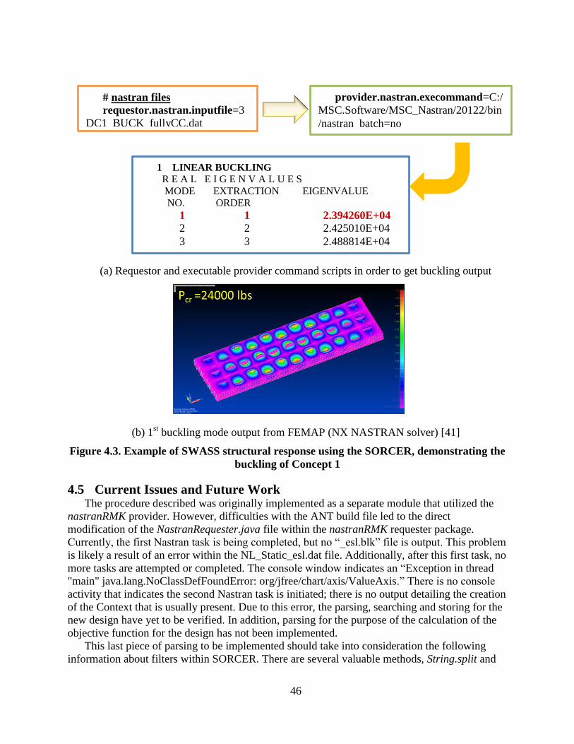
46
provider.nastran.execommand=C:/
MSC.Software/MSC_Nastran/20122/bin
/nastran batch=no
(a) Requestor and executable provider command scripts in order to get buckling output
(b) 1st buckling mode output from FEMAP (NX NASTRAN solver) [41]
Figure 4.3. Example of SWASS structural response using the SORCER, demonstrating the
buckling of Concept 1
4.5 Current Issues and Future Work The procedure described was originally implemented as a separate module that utilized the
nastranRMK provider. However, difficulties with the ANT build file led to the direct
modification of the NastranRequester.java file within the nastranRMK requester package.
Currently, the first Nastran task is being completed, but no “_esl.blk” file is output. This problem
is likely a result of an error within the NL_Static_esl.dat file. Additionally, after this first task, no
more tasks are attempted or completed. The console window indicates an “Exception in thread
"main" java.lang.NoClassDefFoundError: org/jfree/chart/axis/ValueAxis.” There is no console
activity that indicates the second Nastran task is initiated; there is no output detailing the creation
of the Context that is usually present. Due to this error, the parsing, searching and storing for the
new design have yet to be verified. In addition, parsing for the purpose of the calculation of the
objective function for the design has not been implemented.
This last piece of parsing to be implemented should take into consideration the following
information about filters within SORCER. There are several valuable methods, String.split and
# nastran files
requestor.nastran.inputfile=3
DC1_BUCK_fullyCC.dat
1 LINEAR BUCKLING
R E A L E I G E N V A L U E S
MODE EXTRACTION EIGENVALUE
NO. ORDER
1 1 2.394260E+04
2 2 2.425010E+04
3 3 2.488814E+04

47
regx, within NastranOutput.java a class within the nastranRMK provider package. Currently,
this class is configured to parse static and dynamic aeroelastic results and place them into a
NastranObject object. This method is the best candidate to be extended for the purposes of this
project. Additionally, in the BasicFileFilter class is the .getFields method which allows parsing
of bulk data with a comma or fixed field length. Modification to allow the input of the proper
delimiter could make this method viable as well. For further reference, the package containing all
basic filters is located in the directory “iGrid/modules/sorcer/src/sorcer/vfe/filter/.” With this
information concerning filters and resolution of the previously stated error, this module can
likely be completed, tested and committed to the registry in the near future.
4.6 Conclusion This project sought to highlight the advantages of the SORCER environment by
implementing Ricciardi’s Nonlinear Aeroelastic Scaling procedure within the SORCER
environment. Though the module to perform this analysis is not completely finished, the
advantages of SORCER are still apparent. A large library of modules for most aerospace
applications already exists. Built in filters and similar methods provide reading and writing
assistance for a variety of file types and formats. Making full use of the already established and
functioning modules and examples is recommended for a beginning user; most only require a
few changes in the property files to allow provider and requester to be run from one’s machine.
If there is existing source code that can be modified to fit user needs, always modify before
attempting to create a module from scratch. At the very least, one can fall back upon the
serviceProvider_Requester_Template package located in the directory
“iGrid/modules/engineering/apps/.” With these resources and the necessary background
knowledge, most should be able to create and utilize the SORCER environment.
The most difficult part of implementing or simply using existing modules within SORCER
was locating them. Neither the package explorer nor navigator tabs within Eclipse allowed for
easy navigation or search. This problem was only compounded by the manual which often had
blank sections (Java Native Access sections) and was far too technical for a typical engineer’s
entry level of knowledge. Additionally, the wealth of presentations in the notes section were
helpful, but often had large amounts of crossover material and required significant time to comb
through to find useful information. The SORCER environment would benefit greatly from a
centralized index. At the least, the index could include all modules currently available and
functioning along with a short description of its purpose or abilities. A longer description which
described methods or filters developed within the module would also be appreciated. The most
helpful would be instructions of what the user needs to provide or alter. For example, the
readME.txt document included in the module titled “nastran” under “requester/docs” was very
helpful. It is a short paragraph that informs the user of what must be supplied. Ideally, both the
index and every module in the “docs” folder would have a similar paragraph. If such an index
were to be appended to a complete manual which can provide more in depth information for
more experienced user, the SORCER environment would become more accessible to all users.
4.7 Tutorial Links Stanford’s Introduction to Computer Science: Programming Methodology:
<http://see.stanford.edu/see/courseinfo.aspx?coll=824a47e1-135f-4508-a5aa-866adcae1111>
Eclipse Online Tutorial:
<http://eclipsetutorial.sourceforge.net/totalbeginnerlessons.html>

48
Chapter 5 Conclusions and Recommendations
Conclusions
The SWASS was configured by multiphysics modeling to quantify the variation in structural
and electromagnetic performance. This study was accompanied with trade studies involving
structural parameters such as panel thickness, composite laminate layup, stiffener size, shape and
spacing, as well as waveguide parameters such as slot size, and spacing. The achievements are
summarized as follows.
Formulated an integrated multidisciplinary design optimization (MDO) problem statement
that incorporates the multiple objectives of minimizing structural mass and maximizing EM
beam intensity, while satisfying structural constraints on strength and stiffness and EM
constraints on EM beam width, direction and actuating power. Solved the EM sub-problem
initially using RSM.
Finite difference sensitivity calculations were implemented for the aforementioned SWASS
configurations to confirm the extent to which optimality conditions were satisfied by the
approximate optimal designs found using RSM. The computed sensitivities in gradient-based
optimization methods were used to hone in on locally optimal solutions.
Structural design and optimization of the four novel SWASS design concepts were
performed. Classical composite plate theory was employed to construct the equivalent plate
model accompanying smeared effect of slots. For higher fidelity, 3D plate FEM models were
developed for computational cost savings, while maintaining accuracy. The 3D models were
validated against experiments. Computational models and source for SWASS design
optimization were delivered that are compatible and functions with Service ORiented
Computing EnviRonment (SORCER).
Recommendations
In order to advance the multiple structural and EM performances, we propose an integrated
approach to a technology solution for SWASS:
(1) Formulate the parameterization scheme for SWASS design that enhances the combined
electromagnetic and structural performance. This will lead designers to direct the development
by requests of AFRL.
(2) Develop an analytical/numerical methodology that will enable predictions of the complex
radiation patterns. The new methodology, based on a mathematical framework for establishing
and unifying the existing solutions, will compute numerically the multiobjective optimal
problems.
(3) Develop software that integrates low and high complexity design and optimization. The
software shall be appropriate for use by SWASS developers and accommodate progressive
design by use of the SORCER consistent with the system-level design requests.

49
Acknowledgement This material is based on research sponsored by the Air Force Research Laboratory under the
agreement number FA8650-09-2-3938. The U.S. Government is authorized to reproduce and
distribute reprints for governmental purposes notwithstanding any copyright notation thereon.
Regarding the SORCER, the authors would like to thank all those who offered assistance to
this project both at Virginia Tech and at AFRL. Special thanks are due to the following: Scott
Burton of AFRL for all the help debugging, Dr. Raymond Kolonay of AFRL for the valuable
insight on filters, Anthony Ricciardi for providing background on ESL and his process and
Nathan Love who provided the Stanford tutorial.

50
List of References
1. Paul, D., Kelly, L., Venkayya, V., and Hess, T., Evolution of U.S. military aircraft
structures technology. Journal of Aircraft, 2002. 39(1): p. 18-29.
2. Callus, P.J., Conformal Load-Bearing Antenna Structure for Australian Defence Force
Aircraft. 2007: Australia. p. 50p.
3. Lockyer, A.J., Alt, K.H., Coughlin, D.P., Durham, M.D., Kudva, J.N., Goetz, A.C., and
Tuss, J. Design and development of a conformal load-bearing smart-skin antenna:
overview of the AFRL Smart Skin Structures Technology Demonstration (S3TD). in Smart
Structures and Materials 1999: Industrial and Commercial Applications of Smart
Structures Technologies, 2-4 March 1999. 1999. USA: SPIE-Int. Soc. Opt. Eng.
4. Alt, K.H., Lockyer, A.J., Coughlin, D.P., Kudva, J.N., and Tuss, J. Overview of the
DoD's RF Multifunction Structural Aperture (MUSTRAP) Program. in Smart Structures
and Materials 2001: Smart Electronics and MEMS, 5-7 March 2001. 2001. USA: SPIE-
Int. Soc. Opt. Eng.
5. Smallwood, B.P., Canfield, R.A., and Terzuoli Jr, A.J. Structurally integrated antennas
on a joined-wing aircraft. in 44th Structural Dynamics, and Materials Conference. 2003.
Norfolk, VA, United states: American Inst. Aeronautics and Astronautics Inc.
6. Seong Ho, S., Soon Young, E., and Woonbong, H., Development of a smart-skin phased
array system with a honeycomb sandwich microstrip antenna. Smart Materials and
Structures, 2008. 17(Copyright 2008, The Institution of Engineering and Technology): p.
035012 (9 pp.).
7. Skolnik, M.I., Radar handbook. 1990, New York: McGraw-Hill.
8. Stimson, G.W., Introduction to Airborne Radar (2nd Edition). SciTech Publishing.
9. List of Radars. cited 04-19-2010; Available from:
http://en.wikipedia.org/wiki/List_of_radars.
10. Collin, R.E., Foundations for Microwave Engineering (2nd Edition). Wiley-IEEE Press.
11. Balanis, C.A., Antenna Theory - Analysis and Design (3rd Edition). 2005: John Wiley &
Sons.
12. Callus, P.J., Novel Concepts for Conformal Load-Bearing Antenna Structure. 2008:
Australia. p. 111p.
13. Johnson, R.C., Antenna Engineering Handbook (3rd Edition). 1993: McGraw-Hill.
14. Bushnell, D., Theoretical basis of the PANDA computer program for preliminary design
of stiffened panels under combined in-plane loads. Computers and Structures, 1987.
27(Copyright 1988, IEE): p. 541-63.
15. Changyi Su, H.K., Todd Hubing, Overview of Electromagnetic Modeling Software, in
25th Annual Review of Progress in Applied Computational Electromagnetics 2009:
Monterey, California.
16. RF Module User's Guide. 2010, COMSOL Multiphysics.
17. EMSS, FEKO User's Manual. 2013, EM Software & Systems-S.A. (Pty) Ltd.
18. CST MICROWAVE STUDIO cited 04-05-2010; Available from: https://www.cst.com/.
19. ANSYS HFSS. cited 04-05-2010; Available from: http://www.ansys.com/.
20. edaboard. cited 04-05-2010; Available from: http://www.edaboard.com/.
21. E. Johansson, N.K.-W., C. Wikstrom, and S. Wold L. Ericksson, Design of experiments:
principles and applications. 2000: Umetrics Academy.

51
22. Canfield, R.A., Multipoint cubic surrogate function for sequential approximate
optimization. Structural and Multidisciplinary Optimization, 2004. 27(5): p. 326-336.
23. Kolonay, R.M. and Sobolewski, M., Grid Interactive Service-Oriented Programming
Environment, in 11th ISPE International Conference on Concurrent Engineering:
Research and Applications (CE2004). 2004: Beijing, China. p. 90-102.
24. Soblewski, M. SORCER: Computing and metacomputing intergrid. in ICEIS 2008. Tenth
International Conference on Enterprise Information Systems, 12-16 June 2008. 2008.
Madeira, Portugal: Institute for Systems and Technologies of Information, Control and
Communication.
25. Ha, T. and Canfield, R.A. Design Optimization of a WR-90 Slotted Waveguide Antenna
Stiffened Structures in 52nd AIAA/ASME/ASCE/AHS/ASC Structures, Structural
Dynamics and Materials Conference, April 4, 2011 - April 7, 2010. 2011. Denver, CO,
United states: American Institute of Aeronautics and Astronautics Inc.
26. Callus, P.J., Novel Concepts for Conformal Load-Bearing Antenna Structure. 2008,
Defense Science and Technology Organization, Aeronautical and Maritime Research
Laboratory, P.O. Box 4331, Melbourne, Victoria, 3001, Australia. p. 94.
27. Sabat, J.W. and Palazotto, A.N., Structural performance of composite material for a
slotted waveguide antenna stiffened structure under compression. Composite Structures,
2013. 97( ): p. 202-210.
28. Kim, W., Canfield, R.A., Baron, W., Tuss, J., and Miller, J. Modeling and Simulation of
Slotted Waveguide Antenna Stiffened Structures. in 19TH INTERNATIONAL
CONFERENCE ON COMPOSITE MATERIALS. 2013. Montreal, Canada: .
29. Volakis, J.L., Antenna engineering handbook. 2007, New York: McGraw-Hill.
30. Balanis, C.A., Advanced engineering electromagnetics. 1989, New York: Wiley.
31. Elliott, R.S., Antenna theory and design. 2003, Hoboken, N.J.: John Wiley & Sons.
32. MATLAB, Optimization ToolboxTM User’s Guide. 2012.
33. ModelCenter, ModelCenter 8.0 Help. 2008, Phoenic Integration, Inc.
34. Eriksson, L., Johansson, E., Kettaneh-Wold, N., Wikström, C., and Wold, S., Design of
Experiments: Principles and Applications. 2000: Umetrics Academy.
35. Myers, R.H.M., Douglas C.; Anderson-Cook, Christine M., Response surface
methodology : process and product optimization using designed experiments. 2009,
Hoboken, N.J.: Wiley.
36. Kim, W., Ha, T., Canfield, R.A., Baron, W., and Tuss, J., Radio Frequency Optimization
of Slotted Waveguide Antenna Stiffened Structure In preparation.
37. Knutsson, L., Brunzell, S., and Magnusson, H. Mechanical design and evaluation of a
slotted CFRP waveguide antenna. in Fifth International Conference on Composite
Materials, ICCM-V. 1985. San Diego, CA, USA: Metallurgical Soc Inc.
38. Timoshenko, S. and Woinowsky-Krieger, S., Theory of plates and shells. 1959, New
York: McGraw-Hill.
39. Gürdal, Z., Haftka, R.T., and Hajela, P., Design and optimization of laminated composite
materials. 1999, New York: Wiley.
40. Reddy, J.N., Mechanics of laminated composite plates and shells : theory and analysis.
2nd ed. 2004, Boca Raton: CRC Press.
41. FEMAP 10.3. 2011, Siemens Inc.
42. MSC Nastran Quick Reference Guide 2012, in 2012, MSC Software.

52
43. Ricciardi, A.P., Canfield, R.A., Patil, M.J., and Lindsley, N. Nonlinear aeroelastic
scaling of a joined-wing aircraft. in 53rd AIAA/ASME/ASCE/AHS/ASC Structures,
Structural Dynamics and Materials Conference, April 23, 2012 - April 26, 2012. 2012.
Honolulu, HI, United states: American Institute of Aeronautics and Astronautics Inc.
44. Ricciardi, A.P., Eger, C.A.G., Canfield, R.A., and Patil, M.J. Nonlinear aeroelastic
scaled model optimization using equivalent static loads. in 54th
AIAA/ASME/ASCE/AHS/ASC Structures, Structural Dynamics and Materials Conference,
April 8, 2013 - April 11, 2013. 2013. Boston, MA, United states: American Institute of
Aeronautics and Astronautics Inc.
45. Park, G.-J., Shin, M.-K., and Park, K.-J., Optimization of structures with nonlinear
behavior using equivalent loads. Computer Methods in Applied Mechanics and
Engineering, 2007. 196(4-6): p. 1154-67.
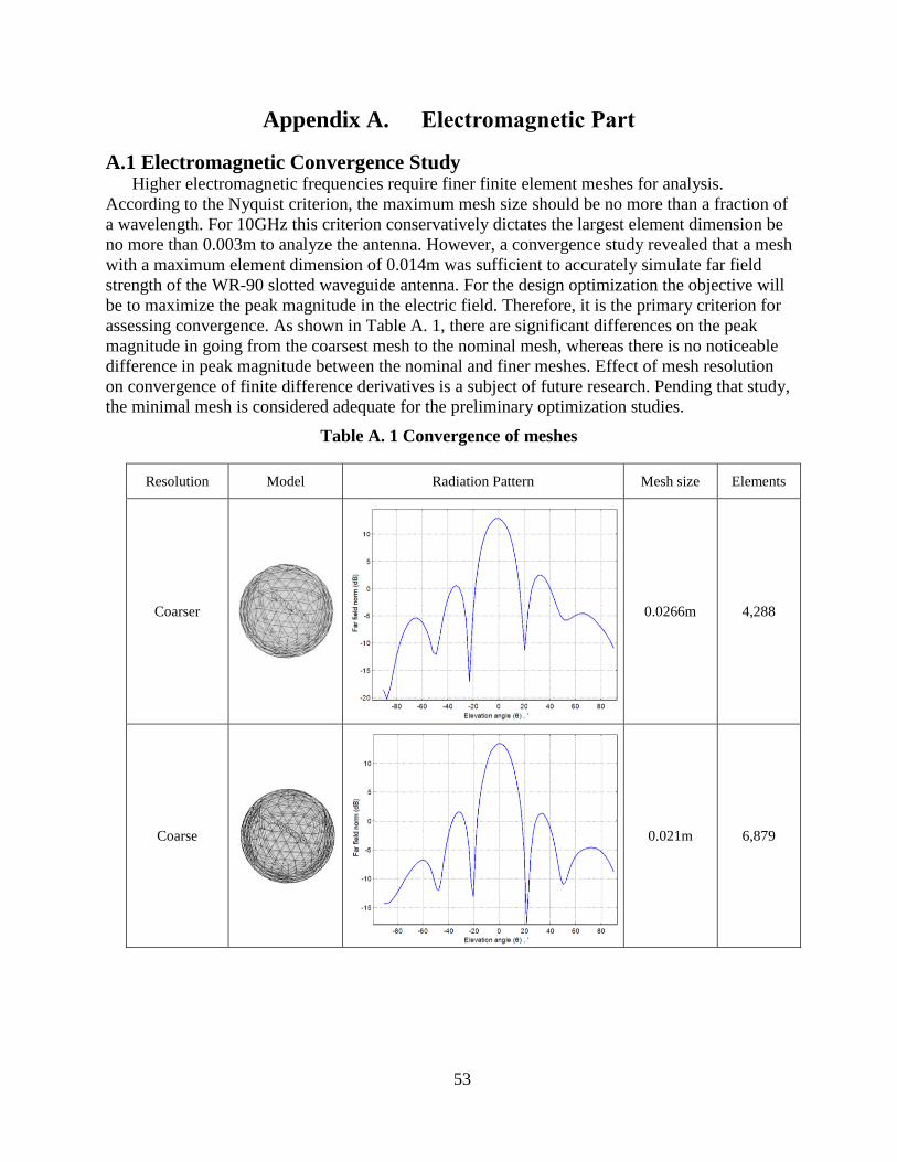
53
Appendix A. Electromagnetic Part
A.1 Electromagnetic Convergence Study Higher electromagnetic frequencies require finer finite element meshes for analysis.
According to the Nyquist criterion, the maximum mesh size should be no more than a fraction of
a wavelength. For 10GHz this criterion conservatively dictates the largest element dimension be
no more than 0.003m to analyze the antenna. However, a convergence study revealed that a mesh
with a maximum element dimension of 0.014m was sufficient to accurately simulate far field
strength of the WR-90 slotted waveguide antenna. For the design optimization the objective will
be to maximize the peak magnitude in the electric field. Therefore, it is the primary criterion for
assessing convergence. As shown in Table A. 1, there are significant differences on the peak
magnitude in going from the coarsest mesh to the nominal mesh, whereas there is no noticeable
difference in peak magnitude between the nominal and finer meshes. Effect of mesh resolution
on convergence of finite difference derivatives is a subject of future research. Pending that study,
the minimal mesh is considered adequate for the preliminary optimization studies.
Table A. 1 Convergence of meshes
Resolution Model Radiation Pattern Mesh size Elements
Coarser
0.0266m 4,288
Coarse
0.021m 6,879

54
Nominal
0.014m 12,807
Fine
0.0112m 21,205
Finer
0.0077m 51,642
Extra fine
0.0049m 201,412

55
A.2 Types of Rectangular Waveguide Standards
Table A. 2. Rectangular waveguide standards
Frequency
band
Waveguide
standard
Frequency
limit (GHz)
Dimensions
Width Height
(inches)
Dimensions
Width Height (m)
F WR-159 4.90–7.05 1.590 0.795 0.04039 0.02019
C WR-137 5.85–8.20 1.372 0.622 0.03485 × 0.01580
H WR-112 7.05–10.0 1.122 0.497 0.02850 × 0.01262
X WR-90 8.20–12.4 0.900 0.400 0.02286 × 0.01016
Ku WR-62 12.4–18.0 0.622 0.311 0.01580 × 0.07900
K WR-51 15.0–22.0 0.510 0.255 0.01295 × 0.00648
K WR-42 18.0–26.5 0.420 0.170 0.01067 × 0.00432
Ka WR-28 26.5–40.0 0.280 0.140 0.00711 × 0.003556

56
Appendix B. Structural Part
B.1 Buckling Analysis of Non-slotted and Slotted Waveguide Tubes
Figure B. 1. Comparison of non-slotted and slotted waveguide tubes.
Concept 1 Concept 2 Concept 3 Concept 40
10
20
30
40
50
60
Four design concept
Cri
tical
bu
ckli
ng
(kip
)
Non-slotted
Slotted

57
(a) Concept 1
(b) Concepts 2 & 3
(c) Concept 4
Figure B. 2. Buckling modes of non-slotted and slotted waveguide tubes.

58
B.2 Interlaminar Shear Stresses
(a) Concept 1
(a) Initial design
(b) Post-optimization
Figure B. 3. Concept 1: Interlaminar shear stress curves. The post-optimization curves
satisfy the interlaminar shear stress requirements at the design load of 12,000 lbf (see
Chapter 3).
-1.5 -1 -0.5 -0.2 0 0.2 0.5 1
x 104
0
12,000
20,000
30,000
40,000
Interlaminar shear stress [psi]
Co
mp
ressiv
e lo
ad
[lb
f]
yz
, 5-6 layer (fully CC)
xz
, 5-6 layer (fully CC)
yz
, 5-6 layer (loosely CC)
xz
, 5-6 layer (loosely CC)
Inter. shear stress limit
Inter. shear stress limit
-2000 -1000 0 1000 20000
12,000
20,000
30,000
Interlaminar shear stress [psi]
Co
mp
ressiv
e lo
ad
[lb
f]
yz
, 6-7 layer (loosely CC)
xz
, 6-7 layer (loosely CC)
Inter. shear stress limit
Inter. shear stress limit

59
(b) Concept 2
(a) Initial design
(b) Post-optimization
Figure B. 4. Concept 2: Interlaminar shear stress curves.
-4000 -3000 -2000 -1000 0 1000 2000 3000 4000 5000 6000 70000
12,000
20,000
30,000
40,000
Interlaminar shear stress [psi]
Co
mp
ressiv
e lo
ad
[lb
f]
yz
, 5-6 layer (fully CC)
xz
, 5-6 layer (fully CC)
yz
, 5-6 layer (loosely CC)
xz
, 5-6 layer (loosely CC)
Inter. shear stress limit
Inter. shear stress limit
-2000 -1000 0 1000 20000
12,000
20,000
30,000
Interlaminar shear stress [psi]
Co
mp
ressiv
e lo
ad
[lb
f]
yz
, 6-7 layer (loosely CC)
xz
, 6-7 layer (loosely CC)
Inter. shear stress limit
Inter. shear stress limit

60
(c) Concept 3
(a) Initial design
(b) Post-optimization
Figure B. 5. Concept 3: Interlaminar shear stress curves.
-3000 -2000 -1000 0 1000 2000 3000 4000 5000 60000
12,000
20,000
30,000
Interlaminar shear stress [psi]
Co
mp
ressiv
e lo
ad
[lb
f]
yz
, 6-7 layer (fully CC), non-load-bearing
xz
, 6-7 layer (fully CC), non-load-bearing
yz
, 6-7 layer (loosely CC), non-load-bearing
xz
, 6-7 layer (loosely CC), non-load-bearing
Inter. shear stress limit
Inter. shear stress limit
-2000 -1000 0 10000
12,000
20,000
30,000
Interlaminar shear stress [psi]
Co
mp
ressiv
e lo
ad
[lb
f]
yz
, 7-8 layer(loosely CC), non-load-bearing
xz
, 7-8 layer (loosely CC), non-load-bearing
Inter. shear stress limit
Inter. shear stress limit

61
(d) Concept 4
(a) Initial design
(b) Post-optimization
Figure B. 6. Concept 4: Interlaminar shear stress curves.
-3000 -2000 -1000 0 1000 2000 30000
12,0000
20,000
30,000
Interlaminar shear stress [psi]
Co
mp
ressiv
e lo
ad
[lb
f]
yz
, 6-7 layer (fully CC), non-load-bearing
xz
, 6-7 layer (fully CC), non load-bearing
yz
, 6-7 layer (loosely CC), non-load-bearing
xz
, 6-7 layer (loosely CC), non-load-bearing
Inter. shear stress limit
Inter. shear stress limit
-3000 -2000 -1000 0 1000 2000 30000
5,000
12,000
20,000
Interlaminar shear stress [psi]
Co
mp
ressiv
e lo
ad
[lb
f]
yz
, 7-8 layer (loosely CC), non-load-bearing
xz
, 7-8 layer (loosely CC), non-load-bearing
Inter. shear stress limit
Inter. shear stress limit