final report for serdp project rc-1649: advanced … · rc-1649: advanced chemical measurements of...
TRANSCRIPT

PNNL-23025
Prepared for the U.S. Department of Energy under Contract DE-AC05-76RL01830
Final Report for SERDP Project RC-1649: Advanced Chemical Measurements of Smoke from DoD-prescribed Burns TJ Johnson RJ Yokelson SK Akagi IR Burling DR Weise SP Urbanski CE Stockwell J Reardon EN Lincoln LTM Profeta A Mendoza MDW Schneider RL Sams SD Williams CE Wold DWT Griffith M Cameron JB Gilman C Warneke JM Roberts P Veres WC Kuster J de Gouw April 2014


PNNL-23025
Final Report for SERDP Project RC-1649: Advanced Chemical Measurements of Smoke from DoD-prescribed Burns
TJ Johnson RJ Yokelson SK Akagi IR Burling DR Weise SP Urbanski CE Stockwell J Reardon EN Lincoln LTM Profeta A Mendoza MDW Schneider RL Sams SD Williams CE Wold DWT Griffith M Cameron JB Gilman C Warneke JM Roberts P Veres WC Kuster J de Gouw April 2014 Prepared for the United States Department of Energy under Contract DE-AC05-76RL01830 and the Strategic Research and Development Program (SERDP) as Project RC-1649 Pacific Northwest National Laboratory Richland, Washington 99352

REPORT DOCUMENTATION PAGE Form Approved
OMB No. 0704-0188 Public reporting burden for this collection of information is estimated to average 1 hour per response, including the time for reviewing instructions, searching existing data sources, gathering and maintaining the data needed, and completing and reviewing this collection of information. Send comments regarding this burden estimate or any other aspect of this collection of information, including suggestions for reducing this burden to Department of Defense, Washington Headquarters Services, Directorate for Information Operations and Reports (0704-0188), 1215 Jefferson Davis Highway, Suite 1204, Arlington, VA 22202-4302. Respondents should be aware that notwithstanding any other provision of law, no person shall be subject to any penalty for failing to comply with a collection of information if it does not display a currently valid OMB control number. PLEASE DO NOT RETURN YOUR FORM TO THE ABOVE ADDRESS. 1. REPORT DATE 18-OCT-2013
2. REPORT TYPE: Final Report
3. DATES COVERED (Oct 2008 – Oct 2013)
4. TITLE AND SUBTITLE Final Report for SERDP Project RC-1649: Advanced Chemical Measurements of Smoke from DoD-prescribed Burns
5a. CONTRACT NUMBER 5b. GRANT NUMBER 5c. PROGRAM ELEMENT NUMBER SERDP RC-1649
6. AUTHOR(S) T.J. Johnson, R.J. Yokelson, S.K. Akagi, I.R. Burling, D.R. Weise, S.P. Urbanski, C.E. Stockwell, E.N. Lincoln, L.T.M. Profeta, A. Mendoza, M.D.W. Schneider, R.L. Sams, S.D. Williams C.E. Wold, D.W.T. Griffith, M. Cameron, J.B. Gilman, C. Warneke, J.M. Roberts, P. Veres, W.C. Kuster, J. de Gouw
5d. PROJECT NUMBER: RC-1649
5e. TASK NUMBER 5f. WORK UNIT NUMBER 7. PERFORMING ORGANIZATION NAME(S) AND ADDRESS(ES)
8. PERFORMING ORGANIZATION REPORT NUMBER
Pacific Northwest National Laboratory, PO Box 999, Richland, WA 99352
PNNL-23025
9. SPONSORING / MONITORING AGENCY NAME(S) AND ADDRESS(ES) 10. SPONSOR/MONITOR’S ACRONYM(S) Strategic Environmental Research and Development Program
SERDP 4800 Mark Center Drive, Suite 17D03 Alexandria, VA 22350-3605 11. SPONSOR/MONITOR’S REPORT NUMBER(S) 12. DISTRIBUTION / AVAILABILITY STATEMENT Unlimited Distribution 13. SUPPLEMENTARY NOTES
14. ABSTRACT Project RC-1649, “Advanced Chemical Measurement of Smoke from DoD-prescribed Burns” was undertaken to use advanced instrumental techniques to study in detail the particulate and vapor-phase chemical composition of the smoke that results from prescribed fires used as a land management tool on DoD bases, particularly bases in the southeastern U.S. The statement of need (SON) called for “(1) improving characterization of…fuel consumption” and “(2) improving characterization of air emissions …under both flaming and smoldering conditions with respect to ... volatile organic compounds, heavy metals, and reactive gases.” The measurements and fuels were from several bases throughout the southeast (Camp Lejeune, Ft. Benning, and Ft. Jackson) and were carried out in collaboration and conjunction with projects 1647 (models) and 1648 (particulates, SW bases).
15. SUBJECT TERMS
16. SECURITY CLASSIFICATION OF: Unclassified
17. LIMITATION OF ABSTRACT
18. NUMBER OF PAGES
19a. NAME OF RESPONSIBLE PERSON Timothy J. Johnson
a. REPORT unclassified
b. ABSTRACT unclassified
c. THIS PAGE unclassified
None 294
19b. TELEPHONE NUMBER (include area code) 509-372-6058
Standard Form 298 (Rev. 8-98) Prescribed by ANSI Std. Z39.18

iii
ABSTRACT
Objectives: Project RC-1649, “Advanced Chemical Measurement of Smoke from DoD-prescribed Burns” was undertaken to use advanced instrumental techniques to study in detail the particulate and vapor-phase chemical composition of the smoke that results from prescribed fires used as a land management tool on DoD bases, particularly bases in the southeastern U.S. The statement of need (SON) called for “(1) improving characterization of fuel consumption” and “(2) improving characterization of air emissions under both flaming and smoldering conditions with respect to volatile organic compounds, heavy metals, and reactive gases.” The measurements and fuels were from several bases throughout the southeast (Camp Lejeune, Ft. Benning, and Ft. Jackson) and were carried out in collaboration and conjunction with projects 1647 (models) and 1648 (particulates, SW bases).
Technical Approach: We used an approach that featured developing techniques for measuring biomass burning emission species in both the laboratory and field and developing infrared (IR) spectroscopy in particular. Using IR spectroscopy and other methods, we developed emission factors (EF, g of effluent per kg of fuel burned) for dozens of chemical species for several common southeastern fuel types. The major measurement campaigns were laboratory studies at the Missoula Fire Sciences Laboratory (FSL) as well as field campaigns at Camp Lejeune, NC, Ft. Jackson, SC, and in conjunction with 1648 at Vandenberg AFB, and Ft. Huachuca. Comparisons and fusions of laboratory and field data were also carried out, using laboratory fuels from the same bases.
Results: The project enabled new technologies and furthered basic science, mostly in the area of infrared spectroscopy, a broadband method well suited to biomass burn studies. Advances in hardware, software and supporting reference data realized a nearly 20x improvement in sensitivity and now provide quantitative IR spectra for potential detection of ~60 new species and actual field quantification of several new species such as nitrous acid, glycolaldehyde, α-/β-pinene and D-limonene. The new reference data also permit calculation of the global warming potential (GWP) of the greenhouse gases by enabling 1) detection of their ambient concentrations, and 2) quantifying their ability to absorb IR radiation.
RC-1649 delivered measurements of fuel consumption (FC) on DoD bases. RC-1649’s main product was hundreds of the best possible measurements of EF for a very broad suite of both trace gases and particulate species from the many fires. The EF were based on measurements at the FSL laboratory and three different southeastern DoD sites. The chief deliverable for each effort was a comprehensive table of emission factors (EF), with the associated tables for the given ecosystem and fire type. The list of species measured in this project is the most extensive smoke characterization achieved to date and is presented in extensive tables of EF, including broken out by vegetation type, e.g. semiarid shrublands, pine understory, etc. Emission ratios (ER) to carbon monoxide (CO) were also derived: These can be used to estimate downwind levels or photochemical changes for certain species by coupling with data from other CO monitors. Multiple measurements of in-plume chemical transformations were also made via airborne sampling. We also made good progress measuring O3 formation and some progress on secondary organic aerosol (SOA) formation. We made the first measurements of initial black carbon (BC) and BC coating rates with non-filter-based techniques for a suite of U.S. prescribed fires, biomass burning BC gets coated much faster (< 1 h) than BC from other sources such as diesel trucks. This affects climate assessments because the coatings increase the absorption of solar radiation by a lensing effect, but they also increase the BC solubility. Increased solubility means the BC has a greater ability to reduce cloud droplet sizes, which causes atmospheric cooling. The coating also increases the rate of removal in the

iv
atmosphere, reducing both the lifetime that the BC can warm the atmosphere and the likelihood of transport to sensitive snow/ice-covered regions.
Many key trace gases (also PM2.5) were measured using nearly identical FTIR-based systems for the laboratory and field fires. By using the same systems we can make a fairly direct comparison of the lab and field data for a suite of many species that includes both organic and inorganic gases, as well as compounds associated with both the flaming and smoldering phases. Comparisons were made knowing that the fire emission factors depend on modified combustion efficiency, i.e. flaming v. smoldering combustion, and ecosystem type. We have confirmed that studying laboratory biomass fires can significantly increase our understanding of wildland fires, especially when laboratory and field results are carefully combined and compared. Much of the unlofted emissions are produced by smoldering combustion making lab studies of great value at characterizing smoldering-phase emissions. A suggestion for future research is the need to develop methods that allow safe real-time fuel consumption monitoring in the field or at least intermittent samples starting shortly after flaming has died down.
Benefits: The greatest benefit can be paraphrased as having “improved characterization of air emissions under both flaming/smoldering conditions for volatile organic compounds and gases.” The analyses presented here provide a set of emission factors for modeling prescribed fire smoke photochemistry and air quality impacts that go far beyond what was previously available. The new set of EF includes data for hazardous air pollutants and numerous precursors for the formation of ozone and secondary aerosol, all useful for model predictions of the amount of smoke produced by prescribed burns. For example, the SC studies also saw faster secondary O3 formation in smoke plumes that mixed with urban emissions, which suggests avoiding smoke plume interaction with sources of NO2 such as from urban areas (e.g. rush-hour traffic or power plants). We also observed the generation of terpene oxidation products in downwind plumes for the first time, as well as fast formation of large amounts of gas-phase organic acids observed post emission. This demonstrates that the plume evolution is strongly influenced by as-yet unidentified species. It now seems unlikely that managers will have to allow for high amounts of SOA when forecasting downwind impacts of their burns. For a few species some EF values were much higher when measured from ground by fixed-position (open-path IR) methods than when measured by actively locating smoke on the ground or in air. This indicates that active sampling methods could be biased in some cases. Careful co-deployment of the roving sampling equipment with the static open path measurement is needed to ensure that the differences are not instrumental. We believe that the airborne IR measurements may best represent overall fire emissions in terms of global model input, but in terms of best representing the combustion-generated gases and respirable particles (including many toxins and carcinogens) to which a person on the fireline is exposed, a fixed open-path system, by virtue of its position on the perimeter, may give better assessment of smoke exposure affecting personnel deployed on containment lines. However, our ground-based IR samplers are also relevant to estimating exposure for personnel who actively engage in extinguishing point sources, e.g. smoldering stumps.

v
Acknowledgments
We would like to thank our sponsors at the Strategic Environmental Research and Development Program (SERDP) for their ongoing support of this project. In particular we would like to thank our program manager for Resource Conservation project RC-1649, Dr. John Hall for his steadfast support that allowed us to accomplish a very interesting project. We would also like to thank the many members of the Technical Advisory Committee (TAC) that made many fruitful suggestions over the course of the project, including planning the “pseudo-wildfire” that ultimately became the Ft. Jackson campaign.
We would like to thank our many collaborators that also made the project so successful, including collaborators at the National Oceanographic and Atmospheric Administration (NOAA), the National Center for Atmospheric Research (NCAR), Colorado State University, the Pacific Northwest National Laboratory (PNNL), the United States Forest Service (USFS) as well as at the University of California Riverside (UCR) and the Georgia Institute of Technology.
The team also thanks several individuals for their assistance in the preparation of this comprehensive report including Ms. Elizabeth Skagen, Mrs. Dawn Johnson and Ms. Krista Archibald. Their dedication and persistence at preparing such a large document is truly appreciated.


vii
Acronyms and Abbreviations
ABS Absorbance (-log(I/Io)) AFB Air Force Base AFTIR Airborne Fourier Transform Infrared Spectrometer AGU American Geophysical Union AI Analog Input AIMMS Aircraft Integrated Meteorological Measurement System AMS Aerosol Mass Spectrometry AP-42 AP-42 Compilation of Air Pollution Emission Factors (EPA) AQ Air Quality ARCTAS Arctic Research of the Composition of the Troposphere from Aircraft and Satellites BEHAVE Fire Behavior Prediction and Fuel Modeling System BB Biomass Burning BC Black Carbon BLM Bureau of Land Management CDC Center for Disease Control CH2CHCHO Acrolein CH3COOH Acetic Acid CH3OH Methanol CH4, Methane CL Combustion Laboratory CL Camp Lejeune (also MCBCL) CLS Classical Least Squares CO Carbon Monoxide CO2 Carbon Dioxide DAID Delayed Aerial Ignition Device DCERP Defense Coastal/Estuarine Research Program (at Camp Lejeune) DoD U.S. Department of Defense DOE U.S. Department of Energy EC Elemental Carbon EF Emission Factor(s) EFPM2.5 Extra-fine Particulate Matter < 2.5 µm EPA Environmental Protection Agency EPA-CMAQ Environmental Protection Agency – Community Multi-scale Air Quality ER Emission Ratios FB Fort Benning FC Fuel Consumption FHA Fort Huachuca FHL Fort Hunter Liggett FID Flame-ionization Detector FEPS Fire Emission Product Simulation (software) FRAMES FRAgments in Managed EcosystemS web site www.nrs.fs.fed.us FSINFO National Forest Service Library catalog FSL U.S. Forest Service Missoula Fire Sciences Laboratory FTIR Fourier Transform Infrared GA Georgia GA Glycolaldehyde GAO Government Accounting Office GC Gas Chromatography

viii
GC-FID Gas Chromatography with Flame Ionization Detection GC-MS Gas Chromatography - Mass Spectrometry GWP Global Warming Potential H2O Water HAPs Hazardous Air Pollutants HCHO Formaldehyde HCOOH Formic Acid HCl Hydrogen Chloride HCN Hydrogen Cyanide HITRAN HIgh Resolution TRANsmission Molecular Absorption Database HONO or HNO2 Nitrous Acid HPHC Harmful and Potentially Harmful Constituents of Tobacco Smoke IOP Intensive Observation Period IR Infrared IVOC Intermediate Volatility Organic Compound LaFTIR Land-based Fourier Transform Infrared Spectrometer MALT Multiple Atmospheric Layer Transmission (software program) MCBCL Marine Corps Base Camp Lejeune MCE Modified Combustion Efficiency MCT Mercury Cadmium Telluride (infrared detector) MM Molecular Mass MODIS Moderate Resolution Imaging Spectroradiometer MVK Methyl Vinyl Ketone N2O Nitrogen Dioxide NBII National Biological Information Infrastructure NC North Carolina NDIR Non-dispersive Infrared (Spectroscopy) NEMR Normalized Excess Mixing Ratio NFDRS National Fire Danger Rating System NH3 Ammonia NIFC National Interagency Fire Center NIOSH National Institute of Occupational Safety and Health NI-PT-CIMS Negative Ion-Proton Transfer-Chemical Ionization Mass Spectrometer NMHC Non-methane Hydrocarbon NMOC Non-methane Organic Carbon NO Nitric Oxide NO2 Nitrogen Dioxide NOx Nitrogen Oxides (NO and NO2 combined) N2O Nitrous Oxide NOAA National Oceanic and Atmospheric Administration NPS National Park Service NSF National Science Foundation O2 Oxygen O3 Ozone OA Organic Aerosol OC Organic Carbon OH Hydroxyl radical OP-FTIR Open path – Fourier Transform Infrared (spectroscopy) OSCAR Quantitative Infrared Evaluation Software OSHA Occupational Safety and Health Administration OVOC Oxygenate Volatile Organic Compound

ix
PAN Peroxyacetyl Nitrate PEL Permissible Exposure Limit PF Prescribed Fires PILS Particle Into Liquid Sampler PIT-MS Proton-transfer Ion-Trap Mass Spectrometer PLS Partial Least Squares PM Particulate Matter PM2.5 Particulate Matter 2.5 µm and smaller PNNL Pacific Northwest National Laboratory PREFIT/REFIT Infrared data (pre-)processing program PTR-MS Proton transfer – Mass Spectrometer QCL Quantum Cascade Laser RSC Residual Smoldering Combustion SERDP Strategic Environmental Research and Development Program SMA Smoke Management Authorities SMP Smoke Management Plan SO2 Sulfur Dioxide SOA Secondary Organic Aerosol SON Statement of Need SP2 Single Particle Soot Photometer STEL Short Term Exposure Limit SVOC Semivolatile Organic Compound TAC Technical Advisory Committee ToF-MS Time-of-Flight Mass Spectrometry TWA Time-weighted Average UCR University of California at Riverside U.S. United States USFS United States Forest Service VAFB Vandenberg Air Force Base VOC Volatile Organic Compounds WAS Whole Air Sampling WF Wildfire WFEFD Wildland Fuels Emission Factor Database WSOC Water – Soluble Organic Carbon


xi
Contents
ABSTRACT .......................................................................................................................................... iii Acknowledgments ................................................................................................................................. v Acronyms and Abbreviations ............................................................................................................... vii 1.0 Chapter 1 ..................................................................................................................................... 1
Introduction to the Study of Chemical Composition of Smoke from Prescribed Fires on Department of Defense [DoD] bases in the Southeastern United States ......................... 1
1.1 Biomass Burning ............................................................................................................. 1 1.2 Fire and Prescribed Fire on DoD Bases .......................................................................... 2 1.3 Prescribed Fire versus Wildfire ....................................................................................... 4 1.4 Emission Ratios and Emission Factors ........................................................................... 7 1.5 Infrared Spectroscopy as Tool for Measuring Biomass Burning .................................... 8 1.6 Overarching RC-1649 Program Objectives..................................................................... 9
2.0 Chapter 2 ..................................................................................................................................... 12 Experimental Plan and Coordination .......................................................................................... 12 2.1 Introduction and Overall Program Structure ................................................................... 12 2.2 Derivation of Emission Factors ....................................................................................... 14 2.3 Chemical Analysis of Smoke—Utilization of IR Spectroscopy ..................................... 15 2.4 Advanced Infrared Spectrometer for Smoke Analysis .................................................... 15
2.4.1 Infrared Spectral Analysis Software—MALT .................................................. 16 2.4.2 Infrared Reference Spectra— Expanded PNNL Database ................................ 17
2.5 Characterization of Fuels ................................................................................................ 18 2.6 Laboratory Burn Experiments ......................................................................................... 20 2.7 Field Burn Experiments—Camp Lejeune, Fort Benning (1648, AFV, Huachuca) ........ 21 2.8 Fusion of Laboratory and Field Experiments .................................................................. 22 2.9 Compilation and Creation of Emission Factors Database ............................................... 23 2.10 Field Burn Experiments—High Intensity Burns on Long Unburnt Stands at Fort
Jackson ............................................................................................................................ 24 3.0 Chapter 3 ..................................................................................................................................... 26
Infrared Spectroscopy for Gas-phase Biomass Burning Detection: Implementation of an FTIR Spectrometer for Smoke Measurements ................................................................ 26
3.1 Infrared Measurements at the Fire Sciences Laboratory ................................................. 26 3.2 FTIR Spectrometer and Software Implementation at the FSL Laboratory ..................... 27 3.3 FTIR Spectrometer Implementation for Airborne Measurements .................................. 32
4.0 Chapter 4 ..................................................................................................................................... 33 MALT Software for Evaluation of Biomass Burning Infrared Spectra ...................................... 33 4.1 The MALT Program ........................................................................................................ 33
4.1.1 Fundamentals of Infrared Spectral Analysis ..................................................... 33
xii
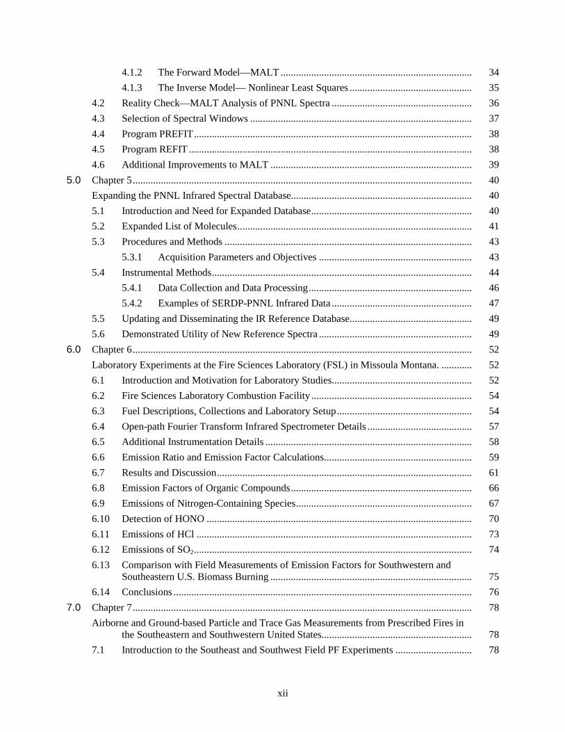
4.1.2 The Forward Model—MALT ........................................................................... 34 4.1.3 The Inverse Model— Nonlinear Least Squares ................................................ 35
4.2 Reality Check—MALT Analysis of PNNL Spectra ....................................................... 36 4.3 Selection of Spectral Windows ....................................................................................... 37 4.4 Program PREFIT ............................................................................................................. 38 4.5 Program REFIT ............................................................................................................... 38 4.6 Additional Improvements to MALT ............................................................................... 39
5.0 Chapter 5 ..................................................................................................................................... 40 Expanding the PNNL Infrared Spectral Database....................................................................... 40 5.1 Introduction and Need for Expanded Database ............................................................... 40 5.2 Expanded List of Molecules ............................................................................................ 41 5.3 Procedures and Methods ................................................................................................. 43
5.3.1 Acquisition Parameters and Objectives ............................................................ 43 5.4 Instrumental Methods ...................................................................................................... 44
5.4.1 Data Collection and Data Processing ................................................................ 46 5.4.2 Examples of SERDP-PNNL Infrared Data ....................................................... 47
5.5 Updating and Disseminating the IR Reference Database ................................................ 49 5.6 Demonstrated Utility of New Reference Spectra ............................................................ 49
6.0 Chapter 6 ..................................................................................................................................... 52 Laboratory Experiments at the Fire Sciences Laboratory (FSL) in Missoula Montana. ............ 52 6.1 Introduction and Motivation for Laboratory Studies....................................................... 52 6.2 Fire Sciences Laboratory Combustion Facility ............................................................... 54 6.3 Fuel Descriptions, Collections and Laboratory Setup ..................................................... 54 6.4 Open-path Fourier Transform Infrared Spectrometer Details ......................................... 57 6.5 Additional Instrumentation Details ................................................................................. 58 6.6 Emission Ratio and Emission Factor Calculations .......................................................... 59 6.7 Results and Discussion .................................................................................................... 61 6.8 Emission Factors of Organic Compounds ....................................................................... 66 6.9 Emissions of Nitrogen-Containing Species ..................................................................... 67 6.10 Detection of HONO ........................................................................................................ 70 6.11 Emissions of HCl ............................................................................................................ 73 6.12 Emissions of SO2 ............................................................................................................. 74 6.13 Comparison with Field Measurements of Emission Factors for Southwestern and
Southeastern U.S. Biomass Burning ............................................................................... 75 6.14 Conclusions ..................................................................................................................... 76
7.0 Chapter 7 ..................................................................................................................................... 78 Airborne and Ground-based Particle and Trace Gas Measurements from Prescribed Fires in
the Southeastern and Southwestern United States........................................................... 78 7.1 Introduction to the Southeast and Southwest Field PF Experiments .............................. 78

xiii
7.2 Experimental Details ....................................................................................................... 79 7.2.1 Site Descriptions ............................................................................................... 79 7.2.2 Airborne Fourier Transform Infrared Spectrometer (AFTIR) .......................... 84 7.2.3 Particulate matter and nephelometry ................................................................. 85 7.2.4 Land-based Fourier Transform Infrared Spectrometer (LaFTIR) ..................... 86 7.2.5 Airborne and Ground-based Sampling Protocols.............................................. 86
7.3 Emission Ratio and Emission Factor Calculations .......................................................... 87 7.4 Results and Discussion .................................................................................................... 88 7.5 Emissions from Understory Fires in Temperate Coniferous Forests .............................. 90 7.6 Emissions from Chaparral Fires ...................................................................................... 94 7.7 Coupled Airborne and Ground-based Measurements ..................................................... 97 7.8 Comparison of Emission Factors (EF) with Compiled Reference Data for
Extratropical Forests ....................................................................................................... 102 7.9 Preliminary Comparison of Field and Laboratory Results .............................................. 103 7.10 Conclusions ..................................................................................................................... 105
8.0 Chapter 8 ..................................................................................................................................... 107 Coupling Field and Laboratory Measurements to Estimate the Emission Factors of
Identified and Unidentified Trace Gases for Prescribed Fires ........................................ 107 8.1 Introduction ..................................................................................................................... 107 8.2 Emissions Measured in the Laboratory and Field Campaigns ........................................ 111
8.2.1 Emissions Measured during Large-scale Laboratory Burning of Biomass ....... 111 8.2.2 Emissions Measured by Airborne and Ground-based Sampling of Field
Fires .................................................................................................................. 114 8.2.3 Fuel Consumption Measurements on Field Fires .............................................. 115
8.3 Data Reduction Approach ............................................................................................... 116 8.4 Results and Discussion .................................................................................................... 119
8.4.1 Comparing the Emissions from Field Fires in Different Fuel/Vegetation Types ................................................................................................................. 119
8.4.2 Comparison of Emission Factors Measured in the Lab and the Field .............. 121 8.4.3 Emission Factors for Prescribed Fires in Temperate Ecosystems ..................... 125 8.4.4 Some Fundamental Characteristics of Fresh Smoke Revealed by Full Mass
Scans ................................................................................................................. 136 8.4.5 Gas-phase Hazardous Air Pollutants Present in Initial Prescribed Fire
Smoke ............................................................................................................... 138 8.4.6 Particle Elemental Carbon Emission Factors and Metal Profiles ..................... 139 8.4.7 Field Measurements of Fuel Consumption on Prescribed Fires ....................... 140 8.4.8 Relevance of Laboratory Fires and Context for this Work ............................... 143
8.5 Conclusions ..................................................................................................................... 144 9.0 Chapter 9 ..................................................................................................................................... 146
Compilation and Creation of Emission Factors Database ........................................................... 146

xiv
9.1 Introduction ..................................................................................................................... 146 9.2 Methods ........................................................................................................................... 146 9.3 Characteristics of the WFEFD ........................................................................................ 148 9.4 Archiving WFEFD .......................................................................................................... 149 9.5 Literature Evaluated for Emissions Data ......................................................................... 152
9.5.1 Database Literature Sources .............................................................................. 152 9.5.2 Additional Literature Evaluated ........................................................................ 155
10.0 Chapter 10 ................................................................................................................................... 169 Biomass Burning Study at Fort Jackson: Atmospheric Emissions and the Effects of High
Intensity Burns on Unmanaged Stands versus the Emissions from Fires Lit During the Wet Season on Frequently Burned Stands ................................................................ 169
10.1 Introduction ..................................................................................................................... 169 10.2 Site Descriptions ............................................................................................................. 172 10.3 Airborne Instrumentation ................................................................................................ 175
10.3.1 Airborne Fourier Transform Infrared Spectrometer (AFTIR) .......................... 175 10.3.2 Whole Air Sampling (WAS) Canisters ............................................................. 176 10.3.3 Other Airborne Measurements .......................................................................... 176
10.4 Ground-based Instrumentation: ....................................................................................... 177 10.4.1 Land-based Fourier Transform Infrared Spectrometer (LAFTIR) .................... 177 10.4.2 Open-path FTIR Spectrometer (OP-FTIR) ....................................................... 177
10.5 Calculation of Excess Mixing Ratios, Normalized Excess Mixing Ratios (NEMRs), Emission Ratios (ERs), and Emission Factors (EFs) ...................................................... 179
10.6 Airborne and Ground-based Sampling Approach ........................................................... 180 10.7 Results and Discussion: Initial Emissions ....................................................................... 183 10.8 Brief Comparison to Similar Work ................................................................................. 192 10.9 Observation of Large Initial Emissions of Terpenes ....................................................... 193 10.10 C3-C4 Alkynes ................................................................................................................. 199 10.11 NH3 .................................................................................................................................. 200 10.12 HCN ................................................................................................................................ 201 10.13 Nitrous Acid (HONO) ..................................................................................................... 203 10.14 Sulfur Containing Species 10.14 ..................................................................................... 203 10.15 Plume Aging .................................................................................................................... 204
10.15.1 Ozone ................................................................................................................ 205 10.15.2 Methanol ........................................................................................................... 207 10.15.3 Formaldehyde.................................................................................................... 208
10.16 Open Path Fourier Transform Infrared (OP-FTIR) Studies ............................................ 210 10.16.1 OP-FTIR Initial Emissions ................................................................................ 210 10.16.2 FTIR Comparison (OP-FTIR, LAFTIR and AFTIR) ........................................ 212 10.16.3 OP-FTIR Comparisons with the Literature ....................................................... 216

xv
10.16.4 Estimating Fire-line Exposure to Air Toxics Using the OP-FTIR Results ....... 217 10.17 Conclusions – Ft. Jackson Study ..................................................................................... 220
11.0 Chapter 11 ................................................................................................................................... 223 Conclusions and Implications for Implementation/Future Research .......................................... 223 11.1 Overview and Summary of Project RC-1649 Results ..................................................... 223 11.2 Advancement of Enabling Technologies and Fundamental Science via RC-1649 ......... 225 11.3 Effects of Prescribed Fire Effluents on Climate Change ................................................. 226 11.4 Synopsis of Lab- versus Field-Measurements and Data Fusion ..................................... 229 11.5 Relevance of findings to land managers .......................................................................... 232 11.6 Suggestions for Future Research and Improved Sampling Schemes .............................. 234

xvi
Figures
1.1 Area burned by wildfire in the U.S. is currently on a rising trend; The historical burned area for the western U.S. sheds light on the burned area trend ................................. 4
1.2 Actual number of acres burned in non-prescribed fires per year for the southern U.S. ........ 5 1.3 Smoke spectrum of the lofted emissions acquired by airborne FTIR is the upper trace
and the smoke spectrum of the RSC emissions acquired by land-based FTIR is the lower trace ............................................................................................................................. 7
2.1 Overview of the project outline including task numbers ...................................................... 14 2.2 A graphical display of the effects of the MALT fitting algorithm ........................................ 16 2.3 Photograph of fuel harvesting at Camp Lejeune for burns conducted at the FSL in
February 2009 ....................................................................................................................... 19 2.4 Evidence of the capability to realistically simulate fires at the FSL combustion facility
for the flaming and smoldering phases of Vandenberg AFB fuels ....................................... 20 2.5 Left: the USFS Twin Otter aircraft. Center: the infrared spectrometer system and
PM instruments in cabin. Right: view from Twin Otter just before entering a smoke plume .................................................................................................................................... 21
2.6 Left: Sampling burning stump emissions with LaFTIR instrument on 30 October 2011. Right: An absorbance spectrum (black) of the fatwood emissions sampled on 30 October ........................................................................................................................ 25
3.1 Schematic of the FTIR coupling to the Fire Sciences laboratory in Missoula ...................... 27 3.2 FTIR, transfer optics, cell entrance and field mirror ............................................................. 28 3.3 Screenshot of the OSCAR software main screen .................................................................. 29 3.4 New Matrix FTIR spectrometer is shown atop the blue table and coupled to the FSL
chimney with the D-mirrors on opposite side of the chimney .............................................. 30 3.5 Signal-to-noise plot of the new dedicated IRCube spectrometer as compared to the
previous laboratory or airborne systems ............................................................................... 31 3.6 Original Midac FTIR spectrometer and coupled White cell used for the airborne
FTIR (AFTIR) measurements ............................................................................................... 32 4.1 A typical MALT fit to the spectral window used to retrieve CO, CO2 and N2O
mixing ratios in smoke .......................................................................................................... 37 4.2 Example of time series of species measured by the FTIR during one fire using the
software programs PREFIT and REFIT................................................................................ 39 5.1 Photographs of IFS 66v spectrometers and gas dissemination systems ............................... 45 5.2 Infrared spectral curve of growth for tetralin displaying 5 of 17 acquired spectra ............... 46 5.3 Composite 298 K infrared spectrum of isovaleraldehyde from 10 individual
measurements ........................................................................................................................ 47 5.4 Composite 298 K infrared spectrum of 2-vinylpyridine from 11 separate
measurements. The y-axis is quantitative and corresponds to an optical depth of 1 ppm-meter ...................................................................................................................... 48
5.5 Absorption spectra of ground samples normalized to the CO absorption band centered at 2143 cm-1 ......................................................................................................................... 50
xvii
5.6 The reference spectra of glycolaldehyde, along with NH3, H2O, and HONO were used to fit smoke spectra in the region of the GA ν10 band near 861 cm-1 .................................... 51
6.1 Schematic of the Fire Lab and photo of a simulation fire in progress .................................. 54 6.2 Time series of selected species measured by the SERDP-built OP-FTIR system,
with strong evidence of emission of several organics during the smoldering phase ............ 61 6.3 Emission factors plotted as a function of modified combustion efficiency for carbon-
containing gas-phase species measured by OP-FTIR for the southeastern and southwestern U.S. fuels......................................................................................................... 65
6.4 Dependence of EF(NOx) on fuel nitrogen content and MCE for chipped understory hardwood, 1-year rough and 2-year rough from Camp Lejeune ........................................... 66
6.5 Contribution of gas-phase nitrogen-containing species to nitrogen balance......................... 69 6.6 Spectral confirmation of the presence of HONO in laboratory biomass fires ...................... 70 6.7 ΔHONO/ΔNOx molar emission ratios for various fuel types .............................................. . 71 6.8 Molar emission ratio of ΔHONO/ΔNOx as a function of altitude for various studies .......... 72 6.9 HCl emission factors by fuel type. See Table 6.1 for fuel descriptions ................................ 73 6.10 Evolution of excess SO2 as a function of excess CO2 and as a function of CO for a
typical fire ............................................................................................................................. 75 6.11 Emission factors for fuels representing various land management strategies at Camp
Lejeune .................................................................................................................................. 76 7.1 Location of the IA and ME prescribed burns at Camp Lejuene ........................................... 81 7.2 Understory fuels observed in the IA and ME prescribed burns at Camp Lejuene ................ 82 7.3 Photograph of the AFTIR system installed in the Twin Otter for Lejeune campaign .......... 84 7.4 Photograph of the LaFTIR in back of pickup sampling burning stumps and burning
live trees on 1 March 2010 at Camp Lejeune ....................................................................... 86 7.5 Emission factors as a function of MCE for the conifer forest understory burns of this
study ...................................................................................................................................... 91 7.6 Emission factors as a function of MCE for chaparral and oak savanna fires of this study
as well as Radke et al. (1991) and Hardy et al. (1996) ......................................................... 96 7.7 Emission factors as measured from both the airborne and ground-based FTIR for the
ME burn of Camp Lejeune, 1 March 2010 ........................................................................... 98 7.8 IR spectra of ground samples normalized to the CO absorption band centered at 2143
cm-1 ....................................................................................................................................... 100 7.9 Comparison of airborne and ground-based emission factors with the recommendations
of Andreae and Merlet (2001) ............................................................................................... 103 7.10 Lower panel –comparison of the average molar ΔHONO/ΔNOx ratios for the various
fuel types studied in this work (airborne) and the laboratory study of Burling et al. (2010). Upper panel – average sum of the molar emission factors of HONO and NOx ....... 104
8.1 Emission factor for acetic acid versus modified combustion efficiency ............................... 108 8.2 The plot shows the EF of vapor-phase methanol vs. MCE from Brazilian forest fires ........ 108 8.3 Time series for CO, CO2, and methanol for an example burn of coastal sage scrub ............ 112 8.4 Comparison of EF versus MCE from the lab and the field fires for smoldering
compounds and PM2.5 for pine understory and semiarid shrubland ...................................... 122

xviii
8.5 Comparison of EF versus MCE from the lab and the field fires for flaming compounds and HCN for pine understory (left column) and semiarid shrubland .................................... 123
9.1 Breakdown of sources of emissions data contained in WFEFD database ............................ 149 9.2 Emissions data distribution by U.S. Forest Service Regions, and Canada ........................... 150 9.3 Screenshot of GUI Format of WFEFD ................................................................................. 151 10.1 Detailed burn maps of Block 6, Block 9b, and Block 22b PFs at Ft. Jackson ..................... 173 10.2 Photos of understory vegetation typical of long-unburnt longleaf pine stands burned
at Ft. Jackson in November 2011 .......................................................................................... 174 10.3 Photograph of the OPAG-22 spectrometer and receiver telescope in the field;
Photograph of sender and receiver telescopes separated by an optical path of ~30 m ......... 178 10.4 Photographs of two examples of the fuels that contributed to residual smoldering
combustion emissions that were sampled by ground-based FTIR and WAS: a live tree base, and dead/down debris ........................................................................................... 180
10.5 Overview of all flight tracks for the Twin Otter aircraft. “RF” indicates research flight ..... 181 10.6 Detailed flight tracks and AFTIR downwind sample locations during RF03 and RF04,
which sampled the Block 9b fire at Fort Jackson on 1 November 2011 ............................... 182 10.7 Detailed flight tracks and AFTIR downwind sample locations during RF07 and RF08
on 7 and 8 November, sampling the Georgetown and Francis Marion fires, respectively ... 182 10.8 Emission ratio plots of ΔCH4/ΔCO from the airborne FTIR multipass cell and
independent RSC targets on the ground from Blocks 6 and 9b, respectively ....................... 184 10.9 Comparison of emission factors from this work with North Carolina work from
airborne and ground-based platforms ................................................................................... 193 10.10 Emission factors of monoterpenes and isoprene measured in this work from ground-
based and airborne platforms ................................................................................................ 197 10.11 C3-C4 alkyne emission factors as a function of MCE from the fires in this study
measured from airborne and ground-based platforms .......................................................... 200 10.12 EF(NH3) as a function of MCE for the South Carolina pine burns of this study
measured from both airborne and ground-based platforms .................................................. 201 10.13 Comparison of ΔHCN/ΔCO study-average emission ratios measured from airborne,
ground-based, and laboratory platforms from five North American studies in pine- forest fuels ............................................................................................................................. 202
10.14 HCN fire-averaged emission factors as a function of MCE for pine/conifer fuel types measured from airborne, ground-based, and laboratory platforms ....................................... 203
10.15 ΔO3/ΔCO NEMR vs. time since emission ............................................................................ 206 10.16 ΔO3/ΔCO vs. time since emission from this study, Yokelson et al. [2009], and Akagi
et al. [2012] ........................................................................................................................... 207 10.17 ΔCH3OH/ΔCO vs. time since emission ................................................................................ 208 10.18 ΔHCHO/ΔCO vs. time since emission ................................................................................. 209 10.19 MCE and excess CO time series from OP-FTIR on the three Fort Jackson fires ................. 211 10.20 Side-by-side comparison of fire-averaged emission factors between the LAFTIR,
OP-FTIR, and AFTIR FTIRs employed during the Fort Jackson campaign ........................ 213 10.21 Emission factors measured by the OP-FTIR, LAFTIR, and AFTIR from the three
Fort Jackson fires: Block 6, Block 9b, and Block 22b ......................................................... 215

xix
10.22 Comparison of emission factors from this work and Wooster et al. (2011) ......................... 216 11.1 Two consecutive infrared spectra of HNCO source output and PNNL reference
spectrum as used to quantify the mixing ratio of isocyanic acid during the 2009 Fire Sciences Lab burns ............................................................................................................... 226
11.2 Plot from PNNL database showing the effects of strong IR cross sections ε(λ) values ....... 228 11.3 Comparison of EF versus MCE from the laboratory and the field fires for smoldering
compounds and PM2.5 for pine understory and semiarid shrubland ...................................... 230

xx
Tables
3.1 Final optimized data collection parameters for data collection using the Matrix IRCube spectrometer for the FSL laboratory and other burns .............................................................. 31
4.1 Retrieved amounts of trace gases by MALT analysis of PNNL reference spectra .................. 37 4.2 Summary of the windows selected for the lab fire analyses .................................................... 38 5.1 List of proposed compounds for IR spectra suggested as part of the biomass burning
IR spectral database ................................................................................................................. 43 5.2 Experimental and Acquisition Parameters associated with the PNNL SERDP database
of infrared reference spectra .................................................................................................... 44 6.1 Summary of vegetation burned and fuel elemental analysis .................................................... 56 6.2 Fuel bed properties for southeastern fuel types burned in laboratory experiment ................... 57 6.3 Instrumentation employed for fire lab simulations fires in February 2009.............................. 59 6.4 Emission factors of gas-phase species for southeastern U.S. and additional fuels .................. 63 6.5 Emission factors of gas-phase species for southwestern U.S.fuels .......................................... 64 7.1 Fire name, location, date, fuels, and size for fires sampled in this study ................................. 80 7.2 Estimated fuel moisture content and fire behavior indices from the 1988 National Fire
Danger Rating System for the prescribed burns at Camp Lejuene and Ft. Jackson ................ 83 7.3 Airborne emission factors and MCE for conifer forest understory burns ................................ 89 7.4 Airborne EF and MCE for chaparral and Emory oak savanna burns in the southwestern
U.S. .......................................................................................................................................... 90 7.5 Statistics for the linear regression of EF as a function of MCE for conifer forest
understory burns and the semi-arid burns of the southwest ..................................................... 92 7.6 Ground-based modified combustion efficiency (MCE) and emission factors for the
2010 Camp Lejeune fires ......................................................................................................... 99 8.1 Summary of the comparison of emission factors measured in the lab and field between
different ecosystems in the field .............................................................................................. 120 8.2 Best estimate emission factors for four types of fire: prescribed fires in semiarid
shrubland and pine-forest understory, and burning coniferous canopy or organic soils .......... 135 8.3 Calculation of some lumped category emission factors in g kg-1 and indicated mass
ratios or percentages ................................................................................................................ 136 8.4 The list of compounds identified in this study that are also considered either hazardous
air pollutants or harmful and potentially harmful constituents in tobacco smoke ................... 139 8.5 Prescribed fire fuel consumption measurements from 1997, 2010, and 2011 for
southeastern U.S. and 2009-2010 for southwestern U.S. ......................................................... 142 9.1 Wildland fire emissions information contained in the Wildland Fuels Emission Factor
Database ................................................................................................................................... 147 9.2 Frequency of occurrence of selected smoke emissions components in the WFEFD ............... 148 10.1 Fire name, location, date, fuels description, size, atmospheric conditions, and burn
history of fires sampled in this Ft. Jackson campaign ............................................................. 174 10.2 Ground-based fuels sampled by LAFTIR and WAS from Blocks 6, 9b, and 22b at
Fort Jackson, SC ...................................................................................................................... 180

xxi
10.3 Ground-based and airborne emission factors and MCE for all South Carolina burns ............. 188 10.4 Statistics for the linear regression of EF as a function of MCE for combined ground-
based and airborne fire-average measurements ....................................................................... 191 10.5 Airborne and ground-based emission ratios of measured terpenes from South Carolina
fires, shown in order of abundance .......................................................................................... 195 10.6 Fire-averaged MCEs and emission factors measured by OP-FTIR for each of the three
pine understory burns at Ft. Jackson ........................................................................................ 210 10.7 Emission factors and MCE for select compounds measured during “early” and “late”
blocks by OP-FTIR .................................................................................................................. 214 10.8 Average TWA and peak exposures measured in this work and other studies and
recommended TWA and peak exposures................................................................................. 218


1
1.0 Chapter 1
Introduction to the Study of Chemical Composition of Smoke from Prescribed Fires on Department of Defense [DoD] bases in the Southeastern United States
1.1 Biomass Burning
Over half of the world’s population employs biomass burning for cooking, heating, lighting, land clearing, fertilizing soils, improving grazing, or other uses [Crutzen and Andreae, 1990]. In developing countries biomass burning is widely-practiced and widely accepted [Hall et al., 1994 Reddy et al., 1997]. As a result, fires are a large source of trace gases and carbonaceous fine particles and they are a major influence on global climate [Andreae and Merlet 2001]. In contrast, in the U.S., biomass burning is practiced by a relatively small number of land managers and much of the public questions the need for burning. However, nationally, “no burning” is not an option as long-term fire suppression merely increases the risk of more-damaging wildfires as described below [Mutch et al., 1994; GAO, 1998]. In fact, the benefits of fire are numerous, including: reduction of hazardous understory fuels; disposal of logging debris; improving access, grazing, and appearance; providing habitat for endangered plant and animal species, and maintaining suitable military training grounds [Wade et al. 1989]. A major challenge for land managers is to garner the benefits of fire without unacceptable air quality impacts. Smoke management is the tool used to achieve this end [Hardy et al. 2001]. The science underlying smoke management is to couple the best available measurements of fuel consumption and emission factors with dispersion models to estimate impacts downwind from a proposed burn and compare the predicted air quality to air quality standards. A proposed burn is then either permitted or canceled: There is little margin for error. Burns from industrial and vegetative sources alone combine to put much of the U.S. near noncompliance for PM2.5 and ozone (O3, a secondary pollutant). In addition, in the United States much of the summertime CO comes from unplanned wildfires in Alaska and Canada [Wotawa et al., 2000]. Only with the best possible data and models can smoke management hope to succeed and preserve the public tolerance for prescribed fire.
Biomass burning is thus a significant global source of trace gases and particles in the atmosphere and has strong impacts on both the chemical composition and radiative balance of the atmosphere [Crutzen and Andreae, 1990]. In the United States, from 1998-2008 the statistical summary prepared by the National Interagency Fire Center which includes the 5 federal wildland agencies and some states suggests that the annual average number of reported wild and prescribed fires was ~80,000 and 14,000, respectively. Also, the average area burned was ~2.6 Mha and 0.9 Mha annually for wild and prescribed fires, respectively (U.S. National Interagency Fire Center, http://www.nifc.gov/fire_info/fire_stats.htm). In 2012, a national survey indicated that prescribed fire use is much more extensive than the NIFC statistics reveal. 2.6 Mha in the southeastern U.S. was burned for forestry objectives in 2011 with an additional 1.5 Mha for agricultural purposes. Nationally, an estimated 3.2 Mha and 5.0 Mha were burned for forestry and agricultural resource objectives, respectively [Melvin, 2012]. In short, prescribed burning of biomass is a commonly used land management tool, with benefits including the reduction of wildfire hazards, improvement of wildlife habitats, removal of harvest debris, and improved access [Biswell, 1999; Wade and Lunsford, 1989]. Many fire-adapted ecosystems depend on the regular occurrence of fire for survival.

2
For biomass burning, the amount of emissions of any compound is affected by many factors, including the combustion processes of the fire (e.g. flaming or smoldering) and also the fuel chemistry, moisture, and geometry (Andreae and Merlet, 2001). The gas-phase emissions from biomass burning are dominated by water vapor (H2O) and carbon dioxide (CO2), but also include significant amounts of many other compounds such as carbon monoxide (CO), nitric oxide (NO), nitrogen dioxide (NO2), methane (CH4), ammonia (NH3), and a multitude of non-methane organic compounds (NMOC) of which oxygenated volatile organic compounds (OVOC) comprise a large fraction [Christian et al., 2003; Christian et al., 2004]. These NMOC may contribute to photochemical ozone [O3] production and secondary organic aerosol [SOA] formation. Gas-phase nitrous acid [HONO] has also been observed in biomass burning plumes both in the laboratory [Keene et al., 2006; Roberts et al., 2010] and in the field [Yokelson et al., 2007a; Yokelson et al., 2009]. While HONO is an important photolytic source of hydroxyl [OH] radicals, the mechanisms of HONO formation are not fully understood [Kleffmann, 2007; Stutz et al., 2010], though HONO has been observed as a direct emission from combustion processes [Finlayson-Pitts and Pitts [2000] and references therein]. It is clear that more research is needed to understand the chemical composition of biomass burning effluents, and their effects on the atmosphere [Crutzen and Andreae, 1990, Hall et al., 1994]
1.2 Fire and Prescribed Fire on DoD Bases
Most DoD bases are in ecosystems that co-evolved with fire as a major natural influence. In the eastern United States, most of the lands managed by DoD are in the southeastern U.S., which was historically dominated by a long-leaf pine savanna maintained by frequent, natural, growing season fires. A lack of fire allows hardwood encroachment that threatens endangered species and limits military training. In addition, in the Southeast, fuel accumulates many times faster than in the rest of the U.S. Thus, only four to six fire-free years can cause a major fuel buildup that makes wildfires more difficult to control and a bigger source of emissions when they do burn [Wade et al., 1989; Hardy et al., 2001; Dept. of Defense Wildland Fire Management Policy Working Group, 1997]. For safety reasons, most of the prescribed fires are now carried primarily during the dormant season (March-May) [www.lejeune.usmc.mil/emd/forestry/suppression.htm ]. Another southeastern U.S. land management concern is the pocosin and other wetland ecosystems: Pocosin is a dense shrub/pine ecosystem that is extremely flammable during drought. It features intense fire behavior when ignited and the fires can be problematic to suppress.
Prescribed burning of wetlands may be shortened in some cases because they are often flooded on a seasonal basis. But removing fire from these ecosystems causes an unnatural buildup of fuels that increases the severity of wildfires, threatens endangered species, and can severely limit DoD training objectives. Thus, carefully planned prescribed fires (PF) have now become a vital land management tool for the DoD (e.g. bases in pine savanna often burn the understory on a ~three year cycle). However, as population increases near the bases, so does the potential that smoke from a prescribed fire might cause undesired air quality impacts for local or regional residents. Moreover, some bases are in areas that are already near non-compliance with federal standards for ozone and fine particles (PM2.5) even before PF are considered. The responsibility for protecting air quality lies mostly with state-level smoke management authorities who ultimately approve or disallow PF. The smoke management team considers the requested burn location and size and combines that with their best estimates of the fuel consumption (FC, mass of fuel burned per unit area), emission factors (EF, mass of pollutant emitted per mass of fuel burned), and smoke dispersion (based on expected injection altitude and forecast winds). A major

3
problem in the whole permitting/PF cycle is that all the necessary estimates were highly uncertain, and in some cases measurements of such data were either few or non-existent for DoD PF. This lack of data contributes a large uncertainty to the air quality predictions and the critical PF programs steered by those predictions.
In 2008, the Strategic Environmental Research and Development Program (SERDP) therefore initiated three projects to characterize smoke chemistry and transport associated with prescribed burns on U.S. DoD lands. The projects focused on prescribed burns in chaparral and Madrean oak woodlands in the southwestern United States and pine forests in the southeastern U.S. Detailed measurements of gaseous and particulate emissions were made in both laboratory and field experiments. The work we describe here has accurately measured both the fuel consumption and the EF of particles and numerous gases, specifically for wildland fuels common on DoD bases. These results promote more accurate air quality predictions, benefiting both the DoD and neighboring communities. This is especially true for DoD PF for which there were very few measurements of any of the above parameters. Post-emission transport and the chemical evolution of smoke were also measured so as to be simulated with photochemical models [Alvarado and Prinn, 2009; Byun and Schere, 2006]. In the laboratory component, fuels representative of vegetation commonly managed by prescribed burning on several southeastern U.S. and southwestern U.S. DoD bases were collected and burned under controlled conditions at the U.S. Forest Service (USFS) Fire Sciences Laboratory in Missoula, Montana. The emissions from these laboratory burns were analyzed with large suite of state-of-the-art instrumentation. The data from these controlled laboratory burns were ultimately synthesized with data from actual field measurements (both airborne and ground-based) of prescribed burns of the same fuels on DoD bases. Thus, the overarching deliverable of our research has been to derive emission factors of the gas-phase species, measured predominantly by infrared spectroscopy in both the laboratory and field.
From the standpoint of producing results directly used by DoD and various smoke management authorities, the main features of SERDP project RC-1649 (as well as RC-1647 and RC-1648) were the intensive observation periods (IOPs), i.e. the laboratory and field experiments. The first of these was an experiment for measuring EF for simulated DoD fires in the USFS large-scale combustion lab using a powerful array of atmospheric chemistry instruments. Specifically, an array of fuels collected from DoD sites in the southeastern and southwestern U.S. during early 2009 were realistically reassembled at the Missoula Fire Lab and burned in a series of 77 fires during February and March, 2009. During each fire, we measured the smoke (and fuel) composition with a comprehensive suite of advanced instrumentation from SERDP projects, as well as from multiple collaborators. Measurements included: filter sampling of particles by numerous complementary collection techniques followed by analyses of metals, ions, and elemental and organic carbon; real-time particle chemistry by aerosol mass spectrometer, particles into liquid samplers, and electrospray mass spectrometry, particle size distribution (including ultrafine nanoparticles) and concentration by numerous complementary techniques; as well as trace gas analysis by open-path Fourier transform infrared, OP-FTIR, and other techniques. The lab fire results are stratified into EF by fuel type (i.e. 1-year rough, pocosin, etc.) and the same was done for the final recommended EF. As detailed below, the lab fires also produced many interesting results, such as the fact that significant amounts of nitrous acid (HONO) were observed by different methods and the results were in excellent agreement with each other. Also, for example, the infrared spectrometer system observed unusually elevated concentrations of hydrochloric acid (HCl) and SO2 from multiple fuels. The second and third observation periods were both field experiments and tried to determine the emission factors

4
from fires typical of the Southeast, representing both prescribed fire (Lejeune 2010) and wildfire (Jackson, 2011).
1.3 Prescribed Fire versus Wildfire
The motivation for both the prescribed fire (EF) and wildfire (WF) studies was that as our RC-1649 program matured, several members of the Technical Advisory Committee (TAC) had suggested trying to better understand the (emission) differences between prescribed fire and wildfire scenarios. This motivation can be understood as follows: Prescribed fire is a widely-used, effective method to reduce forest understory fuel loads and may be needed frequently on the most productive forest sites (e.g. every one to three years). In the southern U.S., several million acres of forest land are treated annually with prescribed fire for multiple resource management objectives. As discussed, the reduced fuel loads are beneficial for many reasons: They minimize the danger of wildfire, improve land access for training, improve forest health, and help to maintain naturally occurring fire-adapted ecosystems. Land managers conduct these burns following guidelines that try to minimize smoke impacts on nearby populated areas. The two main strategies to avoid smoke impacts are: (1) burning when the atmospheric conditions will both vigorously loft the emissions and direct them away from the populated areas, and (2) burning when the fuels are just dry enough to consume the desired amount of fuel (usually 1-3 days after rain), but before the site is so dry that large amounts of forest floor material smolder for prolonged periods, or worse yet, high fire intensity damages the forest overstory.
However, prolonged smoldering after convection from the site has ceased has been defined as “residual smoldering combustion” and is responsible for most of the negative air quality impacts of prescribed fire (e.g. smoke exposure complaints, visibility-limited highway accidents, etc.). Rarely have prescribed fires resulted in major damage to the overstory in what is termed a “stand replacement fire.” One case is the Cerro Grande fire near Los Alamos, New Mexico, which jumped control lines during unexpected high winds in May of 2000 and was finally controlled partly because it burned into an area where the fuel loads had been reduced by previous burning. Wildfires (WF), in contrast, normally burn when “fire danger” is at high levels and forest floor moisture is at a minimum. This often results in significant amounts of RSC and/or stand-replacement fires. Wildfires are typically infrequent on any given site, but when they do occur, they often burn very large amounts of fuel and there are usually few or no options for reducing smoke impacts on populated areas.
Figure 1.1 A) Area burned by wildfire in the U.S. is currently on a rising trend. B) The historical burned area for the western U.S. sheds light on the burned area trend. From 1916-1956 burned area decreased largely due to improved fire suppression which led to increased fuel loading and more intense fires that have been difficult to control even with improved infrastructure. All data from www.nifc.gov. In 2011, 26 x 105 ha were burned in the southeastern region of the U.S. by prescribed fire [Melvin, 2012].

5
Despite the above-mentioned benefits of prescribed fires (PF) over wildfire, PF can occasionally affect air quality, which needs to be recognized and understood. The possibility of unwanted impacts leads to strict regulation of PF (usually by county or state health authorities) and frequent questions by portions of the public as to the value of PF. The justification for prescribed fire is largely based on common sense: All biomass is flammable and eventually the accumulated biomass in any ecosystem is exposed to fire. Experience in the U.S. shows that initial successes in “fire suppression” resulted in greater fuel buildups and consequently fires that are more difficult to control. In fact, the average annual burned area is larger now than before the modern fire suppression era (see Figure 1.1 and Figure 1.2). Thus, the choice land managers face appears to be between two options: option one—prescribed burning of small increments of understory re-growth on a frequent basis with good dispersion, or option two—infrequent, but uncontrolled, burning of massive quantities of biomass with few possibilities to limit population exposures, and also potential damage to watersheds, soil fertility, timber, etc.
Figure 1.2 Actual number of acres burned in non-prescribed fires per year for the southern U.S. http://gacc.nifc.gov/sacc/predictive/intelligence/SA_YTD_firegraphs.jpg. The data for 2010 are for approximately one-half year.
All the above considerations make it appear unwise to oppose a careful, professionally-supervised prescribed fire program, but the justification is based largely on common sense “conventional wisdom”, and the long term trade-offs between the options are difficult to quantify. Only recently have a few ecosystem models addressed some aspects of these trade-offs. For example, one modeling study suggested that the prescribed fire scenario (option 1) leads to more long-term carbon sequestration than option 2. Wiedinmyer et al. [2011] and other current model studies use literature estimates of fuel consumption for the various options. However, fuel consumption data for option 2 (intense fires) is limited and more data of this type were needed. Even less understood is the potential for differences in the chemical composition of the smoke generated by prescribed vs. wild-fires. Given the above descriptions of how these fires behave, the motivation for studying both PF and wildfire can be rephrased in more specific terms: “Is the smoke generated by RSC, high fuel loadings, or “stand replacement” fires chemically different from the smoke generated by lower intensity combustion of above-ground understory fuels at average loadings?” Many corollaries go with this question: If the smoke is different; does it evolve differently in the atmosphere or have different health (physiological) effects on the humans exposed to it? In addressing the question of whether wildfire (WF) and prescribed fire (PF) smoke compositions are different, it can be useful to frame the discussion in terms of six of the major “criteria” pollutants of concern to the EPA namely: CO, O3, NOx, SO2, PM2.5, and lead. Fires emit the first five and the first four are coincidentally measured by FTIR (vide infra).

6
PM2.5 is also a criteria pollutant that can be estimated fairly accurately in fresh smoke from light-scattering measured with the nephelometer on board the Twin Otter, but this is a minimal measurement. Additional PM2.5 can be formed downwind from gas-phase precursors such as NMOC (forms secondary organic aerosols - SOA), NH3 (forms ammonium), SO2 (forms sulfate), and NOx (forms nitrate) and all these precursors are measured by FTIR. The ability to speciate the PM2.5 into the major components such as black carbon (BC), organic aerosol (OA), SOA, chloride, nitrate, ammonium, and sulfate allows a much better assessment of its effects on the global radiation balance and climate. BC absorbs radiation and tends to warm the atmosphere, while OA and the other constituents tend to scatter radiation and cool the climate. If the BC becomes coated by SOA its absorption increases significantly. The inorganic species contribute strongly to the particle solubility and activity as cloud condensation nuclei. But all the particle species, including BC, can cause strong negative climate forcing by influencing cloud droplet size distributions [Reid et al., 2005].
The importance of speciating the PM2.5 should not be underestimated: Because BC is a short-lived climate forcer, the EPA plans to focus on curtailing its emissions. Simply measuring BC might give the impression that BC emitted by fires is “low-hanging fruit” for the mitigation of global warming. In fact, the organic carbon (OC) that is co-emitted with BC by fires causes short-term cooling. The OC/BC ratio for biomass burning is typically 8:1, so curtailing burning to reduce BC would likely have the opposite effect of that intended. The single-particle soot photometer (SP2) is often used to measure BC emissions.
Early work by our project (2009 and 2010) showed that smoke from PF and WF can be significantly different. Such evidence of large differences arose from our ongoing analysis of FTIR spectra acquired in the air and on the ground during the spring 2010 field campaign. In Figure 1.3, the upper traces of parts a – c show different spectral regions of an airborne IR spectrum of smoke generated by the main combustion scenario associated with prescribed fires at an actual prescribed fire at Camp Lejeune in North Carolina on 1 March 2010. Figure 1.3 parts a – c (lower traces) also show the same portions of the IR spectrum, but acquired with our ground-based system and of smoke generated by the minimal amount of RSC that occurred during the same prescribed burn. The spectra are dramatically different. In the airborne spectra, all the species are identified and are familiar compounds associated with biomass burning. We also see high levels of isoprene in the ground-based spectra, but it is absent in the aircraft spectra. There are high NH3 levels in the airborne data, but it is below detection limits in the ground-based data. Figure 1.3b shows that the airborne spectra also have strong peaks due to formaldehyde [HCHO], which are absent from the ground-based spectra. Ammonia and formaldehyde have been seen in ground-based spectra from burning other fuels, but were absent in our limited sampling of RSC in North Carolina southern pine stands. Figure 1.3 shows that the ratio of ethylene and acetylene to CO2 was at least ten times higher in the RSC smoke than in the lofted smoke entrained in the convection column, where the latter should represent nearly all PF smoke. Again, WF smoke could have a much larger fraction [perhaps 50%] of the RSC smoke.

7
Figure 1.3 Smoke spectrum of the lofted emissions acquired by airborne FTIR is the upper trace and the smoke spectrum of the RSC emissions acquired by land-based FTIR is the lower trace. The spectra show that the smoke composition from the two types of combustion can be dramatically different as discussed in the text. The RSC emissions are expected to be much more abundant in wildfires than prescribed fires.
These preliminary findings show a large difference in the suite of NMOC in the lofted and unlofted emissions, which then suggests that a significant chemical difference could exist between WF- and PF-smoke and post-emission O3 production; based on the different RSC contributions expected for these two fire types. Other differences may exist for other emissions or due to combustion in different fuel loadings (larger for WF). Differences may also occur if comparing stand replacement fires to fires that leave the overstory largely unaffected. These PF vs. WF considerations led to an extension of the study by conducting a campaign to analyze smoke constituents from a southeastern U.S. stand that had not been exposed to PF treatment (over 50-year recorded history) and was also burned under dry conditions, i.e. more representative of a true wildfire. This was the motivation for the 2011 Fort Jackson campaign in South Carolina as detailed in Chapter 10.
1.4 Emission Ratios and Emission Factors
During the course of our studies, we consistently report reported both emission ratios [ER] and emission factors [EF]. Excess mixing ratios above background (denoted as ΔX for any species “X”) were calculated for most measurement methods by subtraction of a 60-second average mixing ratio measured prior to the ignition of the fire. Excess mixing ratios were integrated over the whole fire for emission factor and mass balance calculations. Fire-integrated molar emission ratios, ER(X/Y), for species X relative to species Y (usually CO2 or CO), were calculated by:
(1.1)
Emission ratios can be computed for any point in time during a fire [Yokelson et al., 1996], but in this paper we present only fire-integrated emission ratios.
Since the emissions from the various combustion processes [e.g. flaming and smoldering] are different, a useful quantity describing the relative amount of flaming or smoldering combustion is the modified combustion efficiency, MCE, defined as [Yokelson et al., 1996]:

8
(1.2) Higher MCE values indicate more flaming and lower MCE more smoldering combustion. As with emission ratios, MCE can be computed for any point in time during a fire [Yokelson et al., 1996], but here we present only fire-integrated MCE for comparison to fire-integrated emissions.
Fire-integrated emission factors, EF[X] [grams of species X emitted per kilogram dry fuel burned] were calculated by the carbon mass-balance method [Yokelson et al., 1999]:
(1.3) where Fc is the carbon mass fraction of the fuel determined experimentally; MWX is the molecular weight of species X, 12 is the atomic mass of carbon and CX/CT is the number of moles emitted of species X divided by the total number of moles of carbon emitted, given by the following:
(1.4)
where NCj is the number of carbons in species j. Since the majority of the carbon mass [>98-99%] is in the compounds CO2, CO, and CH4 [all of which were measured by OP-FTIR] by considering only the carbon-containing compounds that are detected by the OP-FTIR in the mass balance approach inflates the emission factors by ~1-2% [Yokelson et al., 2007b].
We note that these emission factors EF are the “standard” input to most smoke models, but depend strongly on many parameters such as fuel type, fuel moisture, humidity, burn conditions, etc. The EF are applicable to both gas-phase and particulate-phase species.
1.5 Infrared Spectroscopy as Tool for Measuring Biomass Burning
A most useful technique for the measurement of gas-phase emission factors from biomass burning is open-path Fourier transform infrared [OP-FTIR] spectroscopy. An advantage of OP-FTIR is that the open-path nature of the measurement produces no sampling or storage artifacts, and all compounds are measured simultaneously and path-integrated through the same air parcel. That is OP-FTIR is well suited to measure gases in smoke since it largely eliminates artifacts associated with point sampling, sample storage, and chemical interferences. Other techniques employed for smoke analysis have produced large overestimates of toxic species that led to unjustified concerns about wildland fire. The unique spectral features of the species measured means the technique is resistant to interference and provides unambiguous compound identification. Moreover, OP-FTIR has high temporal resolution for monitoring of dynamic processes related to emissions of biomass fires [Yokelson et al., 1996].
Open path FTIR spectroscopy also provides the possibility to simultaneously measure a wide range of chemical species in smoke with good sensitivity (ppb levels) and high temporal resolution (1-2 sec)
COCOCOMCE
∆+∆∆
=2
2
( )T
XXc C
CMWFkggXEF ×××=12
1000)/(
∑=
∆
∆×
∆∆
=n
j
jj
T
X
COC
NC
COX
CC
1 2
2

9
without the need and uncertainty of sampling the smoke through closed volumes. Since virtually all gases (except notably N2 and O2) absorb infrared light, open-path infrared [IR] spectroscopy is able to quantify most reactive and stable compounds at mixing ratios at or above a few ppbv, depending mostly on spectrometer sensitivity. The only prerequisite is that the IR measurements are based on IR reference spectra that must be acquired in special laboratories with exacting quality control. As part of this project we have therefore expanded the existing PNNL IR database of reference spectra to include more than 50 species associated with the DoD-prescribed burns. Detection of such species is thus enabled.
To further take advantage of such possibilities with IR, in the early stages of the work we developed and deployed a new IR system that is faster and more accurate than those previously available. Open path FTIR measurements of smoke have been made at the fire lab since the early 1990s, firstly during a visiting campaign by Griffith [Griffith, 1991] and subsequently with a dedicated FTIR analyzer [Yokelson et al, 1999]. The new and enhanced sensitivity FTIR spectrometer was key to the laboratory measurements and was dedicated to the existing open path optical system used for cross-stack quantitation of the gas-plume analytes in the FSL combustion facility as described in Chapter 6. The new instrument was later removed from the stack and deployed as the airborne FTIR for the Fort Jackson field study in 2011.
1.6 Overarching RC-1649 Program Objectives
The overarching motivation for the work undertaken by this project RC-1649 was originally summarized in the statement of need by “(1) improving characterization of fuel consumption” and (2) “improving characterization of air emissions under both flaming and smoldering conditions with respect to volatile organic compounds, heavy metals, and reactive gases.” The goal was to provide DoD and civilian smoke managers with the best possible measurements of FC and EF for a broad suite of gases and particulate species emitted by fires on various DoD sites. This should help maximize the use of PF without exceeding air quality standards.
Thus, the research summarized in this report has focused on providing state-of-the-art measurements of fuel consumption (FC) on DoD bases and the best possible measurements of emission factors (EF) for a very broad suite of trace gases and particulate species. Measurements were made at the U.S. Forest Service Missoula Fire Sciences Laboratory (FSL) and at three selected DoD sites or areas, some in conjunction with projects RC-1648 and 1647. A comprehensive table of FC and EF were produced specifically for DoD-relevant ecosystems such as longleaf pine savanna, pine-oak forest, and organic soils. The emission ratios (ER) to carbon monoxide (CO) that we measured can be used to estimate downwind levels or photochemical changes in these species by coupling with data from municipal CO monitors. Measurements of chemical transformations in plumes were also made. The FC and EF data were compared to the available data for natural wildfires to better estimate the benefits of prescribed fire vs. wildfire. The combination of better model input and improved model validation helped decrease situations where the gases and particles emitted by DoD-prescribed burns exceed standards for regulated species, as well as reduce the incidence of burns being inappropriately cancelled. A best effort by DoD to characterize such emissions using state-of-the-art technology should help foster goodwill with the relevant civilian communities.
10
As detailed in the following chapters, the research has quantified the emissions of multiple particulate and gas-phase species emitted by prescribed burns at DoD bases. The measurements have included two distinct research modalities:
1. Three to five burns each for 6 important fuel types (21 total) were carried out at the Fire Sciences Laboratory in Missoula. The fuels for these burns were carefully selected through DoD liaisons to be representative of the ecosystems managed by DoD throughout the Southeast. Five of these burns were selected in conjunction with RC-1647. An additional 49 fuel beds of southwestern fuel types were burned as part of the collaborative effort with RC-1648. The FSL combustion facility has a unique capacity to accurately simulate wildland fires and make emissions measurements that are free of the artifacts that can occur in smaller burning facilities.
2. Airborne and ground-based field measurements were made (at the source and downwind) on DoD-prescribed burns in the southeastern U.S. with simultaneous fuel characterization. The measurements described in objectives 1 and 2 probe both the flaming and smoldering emissions and feature advanced instrumentation that minimizes the sampling and storage artifacts common in smoke analysis.
To achieve measurement objectives 1 and 2 require several integral, broadly-useful technical advances were undertaken. These include:
– Constructing a faster and more accurate infrared spectrometer for the FSL and field measurements,
– Expanding and automating the software algorithm that extracts the gas-phase concentrations from the infrared spectra of smoke, including for the new spectrometer. It is known that IR is capable of quantifying dozens of species, but the data analysis is time-consuming and must be streamlined, and
– Expanding the Pacific Northwest National Laboratory IR database to incorporate numerous key species emitted by DoD biomass burning, notably hazardous air pollutants [HAPs] from the burns.
We note that the ecosystems found at/near Camp Lejeune and Ft. Jackson served as good proxies for the ecosystems that dominate DoD bases throughout the southern U.S. (e.g. Fort Bragg, Eglin AFB, etc.). Fuel moisture, fuel geometry, and fuel consumption were determined at Camp Lejeune for key ecosystems (e.g., pine savanna, pine-oak forest, and organic soils). Fuels were harvested and realistically configured at the large-scale burning facility in the Missoula Fire Sciences Laboratory (FSL) for a series of fires to measure the EF, and emission ratios (ER) to carbon monoxide (CO) and particulate matter (PM) for numerous compounds. The FSL is at ~3300 above sea level; this results in a slightly lower ambient pressure (~659 vs. 760 Torr at sea level), but the effect on combustion is miminal: the mixing ratio of oxygen remains the same regardless of pressure and the combustion efficiency has been measured to be comparable to that observed in the field. The emissions were measured primarily via infrared spectroscopy, but also using nephelometry, filters, mass spectrometry, and chromatography. The EF can be used for state-of-the-art plume modeling for downwind concentrations. The ER allow downwind concentrations to be estimated for numerous compounds by comparison to downwind measurements of CO/PM in affected communities or by comparison with CO and/or PM predicted by dispersion models.

11
However, while laboratory and ground-based measurements are clearly useful, airborne measurements are the best way to probe post-emission chemical transformations in smoke [Goode et al. 2000; Yokelson et al. 2003; Hobbs et al., 2003]. Aircraft are needed to enable sampling both at the source and at any arbitrary downwind location during the brief lifetime (several hours) of a typical PF plume. Tethered balloons or mobile ground-based labs do not provide the flexibility to cope with the spatial extent or uncertainty in plume location associated with real fires. We have found that aircraft measurements of post-emission chemistry are ideal for photochemical model validation [Tabazadeh et al., 2004, Trentmann et al., 2005], and airborne sampling offers the best chance to probe the possible effects of salt spray on smoke plume aerosol formation. Aircraft are also the only efficient way to sample a reasonable number of fires in the field to validate laboratory measurements. Although we have found that laboratory EF agree well with near-source airborne EF, the high expense of airborne work is best reserved for limited validation and probing downwind chemistry. The airborne experiments using the USFS Twin Otter were thus carefully planned (Chapters 7 and 10) to harvest as much plume transformation data as possible.
In summary, the benefits of our work include: better model input data for fuel loading, fuel consumption, and fuel moisture [acquired in the field]; better emission factors [model input] acquired mostly in the Missoula large-scale combustion facility; and better downwind plume data with which to challenge and/or validate smoke chemistry and dispersion models. The outline for the project organization is summarized in Chapter 2, specifics about some of the key technologies used are found in Chapter 3 to 5, and the details results of the studies are found in Chapters 6 to 10.

12
2.0 Chapter 2
Experimental Plan and Coordination
2.1 Introduction and Overall Program Structure
As discussed in Chapter 1, the overarching objective of project RC-1649 is to improve predictions of smoke production, smoke dispersion, and air quality impacts that might result from DoD PF. Concrete objectives are to carry out state-of-the-art measurements of fuel consumption, emission factors, and smoke dispersion to derive improved EF and better predictions. SERDP and DoD are cognizant that prescribed fires represent the only cost-effective way to prevent the buildup of fuel that threatens endangered species, increases the severity of wildfires, and, very importantly, can limit DoD in its ability to meet its training objectives. Since, however, the smoke from a PF may also cause undesired air quality impacts for local or regional residents, SERDP and DoD are thus motivated to better understand the chemical composition of the smoke, both for the gas-phase and particulate species. Better understanding the smoke composition in terms of the emission factors (EF) as described above will help smoke management authorities (e.g. base foresters) better understand the requested burn location and size and combine that with their best predictions of the fuel consumption (FC, mass of fuel burned per unit area), emission factors (EF, grams of pollutant per mass of fuel burned), and smoke dispersion (based on expected injection altitude and forecast winds).
As discussed, the SERDP statement of need specifically calls for “(1) improving characterization of…fuel consumption” and “(2) improving characterization of air emissions …under both flaming and smoldering conditions with respect to ... volatile organic compounds, heavy metals, and reactive gases.” This RC-1649 project has strived to provide state-of-the-art measurements of fuel consumption (FC) on DoD bases and has generated hundreds of the best possible measurements of emission factors (EF) for a very broad suite of trace gases and particulate species. The measurements were made both at the U.S. Forest Service Missoula Fire Sciences Laboratory (FSL) (Chapter 6) as well as at two different DoD sites (described in Chapters 7 and 10) as part of RC-1649 as well as at three other sites in collaboration with RC-1647 and RC-1648. A comprehensive table of EF produced specifically for DoD-relevant ecosystems such as longleaf pine (Pinus palustris) savanna, pine-oak (Pinus spp., Quercus spp.) forest, and organic soils has been generated (Chapter 9). The emission ratios (ER) to carbon monoxide (CO) were also measured and can be used to estimate downwind levels or photochemical changes in these species by coupling with data from municipal CO monitors. Measurements of chemical transformations in plumes have also been made. The EF data have been compared to the available data for natural wildfires to better estimate the benefits of prescribed fire vs. wildfire (Chapters 8 and 11). The combination of better model input and improved model validation should help decrease situations where the gases and particles emitted by DoD-prescribed burns exceed standards for regulated species, as well as reduce the incidence of burns being inappropriately cancelled.
In terms of technical focus points, the research project has quantified the emissions of multiple particulate and gas-phase species emitted by prescribed burns at DoD bases. The measurements included two different types of core research that we term the “intense observation periods (IOPs)”. These include:
1. EF measurements made at the Fires Sciences Laboratory in Missoula during 2009 together with projects RC-1647 and 1648. Typically, five to six burns each were carried out for 15 different fuel

13
types. The fuels for these burns were carefully selected through DoD liaisons to be representative of the ecosystems managed by DoD throughout the southeastern U.S. The FSL facility has a unique capacity to accurately simulate wildland fires and make emissions measurements that are free of the artifacts that can occur in smaller burning facilities. This is detailed in Chapter 6.
2. Airborne and ground-based field measurements were conducted (at the source and downwind) on DoD-prescribed burns in the eastern U.S. with simultaneous careful characterization of the fuels. This includes fires measured in spring of 2010 at Camp Lejeune (Chapter 7), as well high-intensity burns in 2011 on Fort Jackson stands that had not previously been exposed to PF (Chapter 10). The measurements in both these field experiments probed both the flaming and smoldering emissions and feature advanced instrumentation that minimizes the sampling and storage artifacts common in smoke analysis, as well as probes aerosol formation effects in presence of salt spray.
The measurements described in objectives 1 and 2, however, required several integral, broadly-useful technical advances that are best characterized as enabling technologies. These include:
– Constructing a faster, more sensitive and more accurate infrared spectrometer for the FSL and field measurements. The same spectrometer was in fact used in the Fort Jackson experiments. Its development is described below in Chapter 3.
– Expanding and automating the software algorithm (MALT) that extracts the gas-phase concentrations from the infrared spectra of smoke, including for the new spectrometer. It is known that IR is capable of quantifying dozens of species, but the data analysis was previously time-consuming and had to be streamlined. This is described in the ensuing Chapter 4.
– Expanding the Pacific Northwest National Laboratory IR database to incorporate numerous key species emitted by DoD biomass burning, notably hazardous air pollutants (HAPs) from the burns. This work is described in Chapter 5.
The measurement phases were thus conducted to quantify fuel consumption in the field, emission factors in the lab and field, and smoke dispersion in the field. The main advantage of the laboratory component was its ability to use advanced instruments that are not easily field-deployable, e.g. certain types of mass spectrometers. Both the laboratory and field components featured specialized, remote-sensing instrumentation optimized for quantifying reactive species. The goal was to quantify the emissions of multiple particulate and gas-phase species emitted by prescribed burns at DoD bases with the three measurement phases described in Chapters 6, 7, and 10. The execution structure as to how the outlined tasks are linked to one another is depicted in Figure 2.1. The figure is an overview of the project outline: The boxes in black outline represent the work due to the blended proposals and efforts including RC-1647 (Prof. Odman) and RC-1648 (Drs. Miller and Cocker). Many other scientists and collaborators have participated in both the laboratory and field experiments using other funding sources. For the blended proposal projects, these are the projects of Prof. Odman (RC-1647) to whom we provided all the EF and FC data from the lab and field burns in southeastern U.S. fuels for incorporation into his regional air quality model. Also as part of this collaboration, Jim Reardon obtained several fuel samples from Fort Benning in Georgia for the FSL burns of February 2009. These burns provided EF for Fort Benning fuels (Pinus taeda, P. echinata, P. elliottii, P. palustris) that are otherwise not available, as RC-1647 has a limited experimental scope. We also note that while Lejeune and Benning are both southeastern, U.S. bases, there may be differences in the EF, as the understories in these two ecosystems differ significantly. The second collaboration was with Dr. Miller, Dr. Cocker and co-workers at UCR (RC-1648). Both 1649
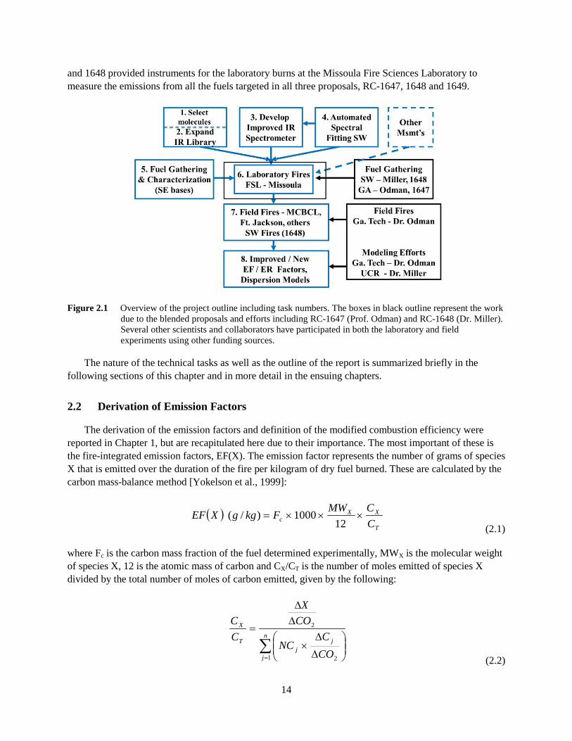
14
and 1648 provided instruments for the laboratory burns at the Missoula Fire Sciences Laboratory to measure the emissions from all the fuels targeted in all three proposals, RC-1647, 1648 and 1649.
Figure 2.1 Overview of the project outline including task numbers. The boxes in black outline represent the work due to the blended proposals and efforts including RC-1647 (Prof. Odman) and RC-1648 (Dr. Miller). Several other scientists and collaborators have participated in both the laboratory and field experiments using other funding sources.
The nature of the technical tasks as well as the outline of the report is summarized briefly in the following sections of this chapter and in more detail in the ensuing chapters.
2.2 Derivation of Emission Factors
The derivation of the emission factors and definition of the modified combustion efficiency were reported in Chapter 1, but are recapitulated here due to their importance. The most important of these is the fire-integrated emission factors, EF(X). The emission factor represents the number of grams of species X that is emitted over the duration of the fire per kilogram of dry fuel burned. These are calculated by the carbon mass-balance method [Yokelson et al., 1999]:
(2.1)
where Fc is the carbon mass fraction of the fuel determined experimentally, MWX is the molecular weight of species X, 12 is the atomic mass of carbon and CX/CT is the number of moles emitted of species X divided by the total number of moles of carbon emitted, given by the following:
(2.2)
( )T
XXc C
CMWFkggXEF ×××=12
1000)/(
∑=
∆
∆×
∆∆
=n
j
jj
T
X
COC
NC
COX
CC
1 2
2
15
where NCj is the number of carbons in species j.
Research over the last 20 years [Yokelson et al., 1996] has shown that the emissions, both gas-phase and particulate, are significantly different for the various combustion processes or fire phases, i.e. flaming vs. smoldering. A useful quantity describing the relative amount of flaming vs. smoldering combustion has been defined as the modified combustion efficiency, MCE, given by
(2.3)
Higher MCE values indicate more flaming and lower MCE more smoldering combustion. As with emission ratios, MCE can be computed for any point in time during a fire, but here we present only fire-integrated MCE for comparison to fire-integrated emissions.
2.3 Chemical Analysis of Smoke—Utilization of IR Spectroscopy
The best measurements of fire EF in recent years have employed infrared (IR) spectroscopy. Open-path or careful extractive IR measurements can avoid most interferences and sampling artifacts as well as all storage artifacts [Griffith et al., 1991; Goode et al. 1999, 2000; Yokelson et al. 1996, 1999, 2003a, b]. Since virtually all chemicals absorb infrared light, IR spectroscopy is one of the most comprehensive techniques available. Other techniques typically target only a few compounds and often produce erroneous results in complex mixtures (such as smoke) due to chemical interference or chemical transformation during sampling/storage. For example, conventional techniques caused big overestimates of the hazardous air pollutants ozone and acrolein in smoke [Pitts et al., 1976; Reinhardt et al., 1994], while [relatively harmless] ammonia and acetic acid were underestimated [Yokelson, 1999]. However, as described in Chapter 1, OP-FTIR is one of the few techniques (along with e.g. mass spectrometry) that allows for the simultaneous measurement of a wide range [dozens, or even hundreds] of chemical species in smoke with reasonable sensitivity (to the ppb level). The method also provides good temporal resolution (as fast as 1 sec) without the added unknown of sampling the smoke through closed volumes or letting the reactive species come in contact with various surfaces.
To take full advantage of IR detection, several enabling technologies were developed. These are outlined in turn, and in some cases discussed in later chapters.
2.4 Advanced Infrared Spectrometer for Smoke Analysis
One of the essential accomplishments that enabled many advances to the science was that we developed and deployed a new IR system that is faster and more accurate than that previously available. The new and enhanced sensitivity FTIR spectrometer was a key to the success of the laboratory measurements. It was a dedicated system and was interfaced to the existing open path mirror system. It was used for cross-stack quantitation of the gas-plume analytes in the FSL combustion facility and it specifics are described in Chapter 3. The new instrument was in the early stages dedicated to the existing open path optical system used for cross-stack quantitation of the gas-plume analytes in the FSL combustion facility (Chapter 3 and Chapter 6). The new instrument was designed and installed under the direction of Prof. Griffith at the University of Wollongong in Australia. The new spectrometer features an interferometer with a flex-pivot mechanism that moves about its own center of mass and is therefore more
COCOCOMCE
∆+∆∆
=2
2

16
robust against shock, shear, or jolts. This led to lower-noise spectra and consequently better detection limits.
2.4.1 Infrared Spectral Analysis Software—MALT
In addition to the hardware described in Chapter 3, the quantitative analysis spectral software was automated and online algorithms were also developed to provide real-time analysis of complex gas mixtures as described in Chapter 4. The latter represents a benchmark improvement, because previously each compound was analyzed separately in a careful, laborious but extremely time-consuming manner. The collected spectra are analyzed after the measurements with the newer faster software to quantify the numerous other trace gas species that are seen in the spectra. Among its principal advantages are that numerous species can be determined simultaneously and that calibration gases are not required, only reference data. Both the hardware and software development accomplished in this project represent an enormous cost savings over a standard FTIR system as far more information (Chapters 6 to 10) has been delivered in far less time. The software is termed MALT and stands for Multiple Atmospheric Layer Transmittance, and is described in detail in Chapter 4 and [Griffith, 1996]. Succinctly put, MALT is a program to retrieve concentrations of trace gases in air or smoke from their FTIR spectra. In the MALT method, spectral regions or “windows” containing peaks of interest are identified, and reference spectra (recorded in other laboratories) are used to account for all the gases absorbing in these windows. The reference spectra are coupled into a model that also fully accounts for minor differences between our OP-FTIR and the reference instrument. The model is run iteratively until a set of gas concentrations that best fits the OP-FTIR smoke spectrum is obtained. An example is seen in Figure 2.2 where CO, CO2, N2O and H2O have been quantified. In this figure, the red trace is the measured experimental spectrum of a Fort Jackson fire, the blue trace (nearly indistinguishable under the red trace) is that fitted to it by MALT, and the green trace above is the residual.
Figure 2.2 A graphical display of the effects of the MALT fitting algorithm. In this case, the algorithm has accurately identified and quantified CO, CO2, H2O and N2O. The simulated spectrum is an optimized composite of the four reference spectra. The residual is at top.

17
Fully automated, the program takes less than one second per analyte spectrum. For smoke, we have shown that results obtained in this fashion agree quantitatively over a wide range of concentrations with reference methods for numerous species such as CO2 and CH3OH [Christian et al., 2004]. So long as the reference data are available, the approach requires no lengthy calibration phase, and is capable of determining many gas species simultaneously, even if their absorption bands overlap. To calculate the contribution of each absorbing species in any spectral region, however, we require quantitative reference spectra such as those in the PNNL library (Chapter 5). Typically, the MALT method provides a precision of better than 1% and absolute accuracies within a few percent for a wide range of species. An example of how a measured broadband experimental infrared spectrum can be used to derive the concentrations of multiple analytes is presented in Figure 2.2.
During the course of the RC-1649 project we made some critical improvements to MALT that have accelerated the program and improve the accuracy of quantifying our smoke measurements:
1. Modifications to the MALT spectral model were required to account for differences between the pressure and temperature of the reference spectra (1013 hPa, 23ºC) and ambient conditions in the IFSL measured spectra (ca. 900 hPa, 20-70ºC), and differences in the buffer gases (air vs. N2).
2. Spectral regions were optimized for the analysis of each new target species.
3. For species where both HITRAN and PNNL reference data are available (e.g. CO2, CO, CH4, NO, NO2, HCN and others), systematic comparisons were carried out and the accuracy assessed.
4. New spectra of species generated in the PNNL library (Chapter 5) were imported into MALT.
5. All spectral analyses were incorporated into both online (i.e., real-time) and offline automated spectral analysis procedures to provide automated analysis of sets of spectra for all desired gases.
2.4.2 Infrared Reference Spectra— Expanded PNNL Database
As described in the previous sections, the only prerequisite to using the new dedicated IR spectrometer and the associated MALT software for analysis for the IR spectra is the availability of infrared reference spectra with which these laboratory and field data can be evaluated. Such reference spectra must be acquired in special laboratories using vetted procedures with exacting quality control. As part of the present project we have thus expanded the existing PNNL IR database of reference spectra to include more than 50 species associated with the DoD-prescribed burns, enabling detection of such gases.
The PNNL infrared spectral library was first created in 2000 and was sponsored by the U.S. Department of Energy for monitoring energy production gases as well as for homeland security applications. While the library contains hundreds of atmospheric species of common interest (e.g. H2O, SO2, NOx, freons, CH3OH) as well as some species known to be products of biomass burning such as alkenes, NH3, HCHO and CH3COOH, the IR database was not funded by DOE as a general tool for atmospheric chemistry or biomass burning science. As a consequence, a major task of RC-1649 was to expand the database to include those species thought to be, or likely to be, found in biomass burning smoke plumes. As detailed in Chapter 5, the species were carefully selected, and more than 50 additional reference spectra were recorded. The protocols, methodologies, and list of spectra are also summarized in Chapter 5.

18
2.5 Characterization of Fuels
Fuel loading and consumption, at any site can be measured by complete weighing of the biomass pre- and post-fire. However, an intensive fuel inventory for every management unit is impractical. The approach used during the Camp Lejeune and Fort Jackson campaigns was to sample the range of fuel loading and fuel consumption associated with different vegetation and environmental conditions [Hessburg et al., 2000]. This increases our understanding of the fuel and fire behavior dynamics. Fuel inputs in the current burning permit program are normally based on undocumented regional estimates or fuel models developed for fire behavior and fire danger rating models [Ottmar and Sandberg 2001]. The actual fuel loadings of proposed burn areas might vary significantly from the available estimates and the use of inaccurate loadings is an important management concern. Burning with higher loadings than reported may produce greater emissions than expected and result in unanticipated health and safety issues. In contrast, reporting higher loadings than actually present might unnecessarily prevent burning or restrict the amount of acres permitted to burn. Reducing burn size results in increased per acre costs.
Three vegetation communities with frequent fire return intervals were characterized in this study using fuel gathering methods. Fuel sampling units were selected from those scheduled for treatment under the current Prescribed Burning Prioritization model in use at Lejeune. Longleaf pine savanna communities have low live fuel loadings dominated by oak and wiregrass (Aristida stricta), significant loads of pine needle litter, and low amounts of down dead woody fuel. In contrast, High or Tall Pocosin shrub-dominated communities have fuel loadings that are dominated by a significant live fuel component, and leaf litter, duff, and suspended 1- and 10-hour fuels. Also of interest are vegetation communities with above average fuel loadings due to fire suppression activities, typically dominated by a pine overstory with a hardwood mid/understory and are expected to have an increased proportion of suspended-dead and down-dead fuels.
The available fuels depend strongly on the type of vegetation community. Standard sampling methods were therefore adapted to address differences in productivity and fuel structure. Fuel loading was estimated in several categories: herbaceous fuel; litter and duff; and suspended or down, dead, woody fuel. Down dead woody fuel was further stratified into 1 hour, 10 hour, 100 and 1000 hour classes. These classes correspond to the standard moisture time lag classes used in the National Fire Danger Rating System, BEHAVE, fire behavior model and other fire modeling programs.

19
Figure 2.3 Photograph of fuel harvesting at Camp Lejeune for burns conducted at the FSL in February 2009. The harvest shows at typical 1-meter-square plot being harvested for a pocosin sample.
Pre- and post-burn fuel loading measurements were conducted following standard sampling procedures [Brown 1974, Lutes 2000]. Owing to the fuel structure differences and spatial variability, a combination of transect and fixed area sampling techniques were needed to fully quantify the fuel loadings. Pre- and post-burn sampling of live fuel, suspended dead fuel, and litter/duff on all sites were measured using paired one-square meter plots. Pre-burn samples were collected from one of the plots, oven dried and weighed. Post-burn fuels were measured on the paired, previously untouched meter plot. Because of the spatial variation associated with burning litter and duff, consumption of these fuels will also be measured using ‘duff pins’, i.e. metal rods inserted into the soil that serve as a reference for pre- and post-burn litter and duff depth measurements. An example is seen in Figure 2.3 for the 2009 FSL burns and the fuels gathered at Camp Lejeune by Jim Reardon and three Forest Service colleagues. In the figure, the harvest is a standard 1 meter square plot for a pocosin sample. During the harvest multiple fuel types were collected including: One year rough (10 samples), Two year rough (15 samples), Pocosin (15 samples), Untreated (22 samples) and Treated (10 samples). No attempts were made to estimate the necessary sample size to achieve a specified level of sample error because of large sample variability and the impracticality of collecting such a large sample given the limited access to the burn sites. The number of samples collected per fuel type is similar to that used to develop fuel loading information for photo series [e.g. Ottmar and Vihnanek, 2000]. Our ability to sample fuels at Ft. Jackson was even more limited.
Because the collection, drying and weighing of large amounts of down dead woody fuel is impractical, the loading of these fuels was estimated using the planar transect inventory method [Brown 1974]. The estimation of fuel/acre is based on the number of intersections of the down-woody (time lag) classes along the transect length. Fuel volume is converted to weight by the specific gravity of sound wood. Down woody fuel consumption was estimated by the post-burn measurement of the transects. In collaboration with Dr. Odman, we also characterized fuels from Fort Benning, with a somewhat different

20
understory. Representative fuel samples of each vegetation type were collected and shipped overnight for burning in the combustion lab at the FSL in Missoula; more details of the burns are found in Chapter 6.
2.6 Laboratory Burn Experiments
The Missoula FSL combustion laboratory is the world’s largest controlled-environment, biomass-burning facility. Because of the available space, the actual fuels in the field can be carefully documented and sampled, followed by a proper spatial reassembly in the FSL. Only here has it been demonstrated that natural fires are realistically simulated [Yokelson et al., 1999; Christian et al., 2003], as seen for fuels from Vandenberg AFB burning in Figure 2.4. Other combustion facilities typically do not provide sufficient space for a realistic configuration of the fuels, which often lay tightly bunched in a pile, thus affecting the combustion process. Once smoke is produced in these smaller facilities, it is often stored at unnaturally elevated temperatures that promote formation of dioxins [Gullet and Touati, 2003] and other air toxics - or it is transformed through excessive contact with metal surfaces. Although the importance of sampling real fires in the field is obvious (especially for probing downwind chemistry), accomplishing representative sampling of field fires is very challenging [Yokelson, 2003]. Thus, there are important advantages to sampling at the FSL: (1) Airborne and ground-based field sampling methods can overestimate the emissions from flaming and smoldering combustion, respectively [Bertschi et al. 2003], but in the FSL lab all the smoke produced from the entire burn is sampled. (2) 2000 kg of instrumentation, including open-path IR and other instruments, can be quickly deployed to allow for comprehensive measurements at relatively low cost [Christian et al., 2003]. (3) Burns are readily scheduled and not subject to costly delays from weather, for example. (4) Emissions can be measured for “pure” flaming or smoldering combustion phases, which is useful in scaling predictions.
Figure 2.4 Evidence of the capability to realistically simulate fires at the FSL combustion facility for the flaming and smoldering phases of Vandenberg AFB fuels
As discussed, open path-Fourier transform infrared (OP-FTIR) spectroscopy is a key technique used at the Fire Sciences lab. Since the measurement is based on passing IR radiation through the smoke, the plume gases are measured in real time without having to come in repeated contact with the surface of any storage or analytical device Thus, OP-FTIR is completely free of sampling and storage artifacts. At the FSL, the OP-FTIR measures completely across the sampling stack ~15 m above the fuel bed. The fuels from Camp Lejeune and Fort Benning were carefully reassembled in the burn facility based on photographs and mass/acre measurements. Burns and measurements were observed by Reardon, Becker,
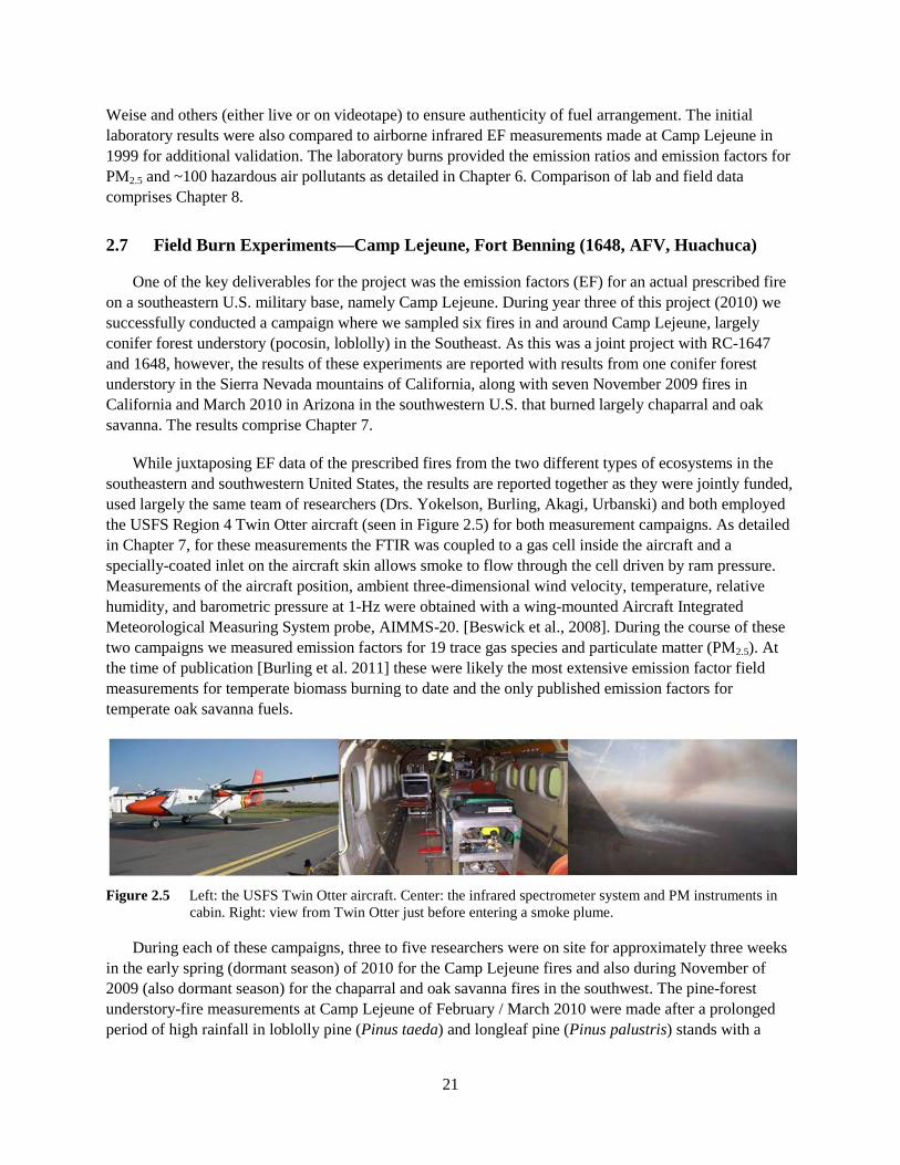
21
Weise and others (either live or on videotape) to ensure authenticity of fuel arrangement. The initial laboratory results were also compared to airborne infrared EF measurements made at Camp Lejeune in 1999 for additional validation. The laboratory burns provided the emission ratios and emission factors for PM2.5 and ~100 hazardous air pollutants as detailed in Chapter 6. Comparison of lab and field data comprises Chapter 8.
2.7 Field Burn Experiments—Camp Lejeune, Fort Benning (1648, AFV, Huachuca)
One of the key deliverables for the project was the emission factors (EF) for an actual prescribed fire on a southeastern U.S. military base, namely Camp Lejeune. During year three of this project (2010) we successfully conducted a campaign where we sampled six fires in and around Camp Lejeune, largely conifer forest understory (pocosin, loblolly) in the Southeast. As this was a joint project with RC-1647 and 1648, however, the results of these experiments are reported with results from one conifer forest understory in the Sierra Nevada mountains of California, along with seven November 2009 fires in California and March 2010 in Arizona in the southwestern U.S. that burned largely chaparral and oak savanna. The results comprise Chapter 7.
While juxtaposing EF data of the prescribed fires from the two different types of ecosystems in the southeastern and southwestern United States, the results are reported together as they were jointly funded, used largely the same team of researchers (Drs. Yokelson, Burling, Akagi, Urbanski) and both employed the USFS Region 4 Twin Otter aircraft (seen in Figure 2.5) for both measurement campaigns. As detailed in Chapter 7, for these measurements the FTIR was coupled to a gas cell inside the aircraft and a specially-coated inlet on the aircraft skin allows smoke to flow through the cell driven by ram pressure. Measurements of the aircraft position, ambient three-dimensional wind velocity, temperature, relative humidity, and barometric pressure at 1-Hz were obtained with a wing-mounted Aircraft Integrated Meteorological Measuring System probe, AIMMS-20. [Beswick et al., 2008]. During the course of these two campaigns we measured emission factors for 19 trace gas species and particulate matter (PM2.5). At the time of publication [Burling et al. 2011] these were likely the most extensive emission factor field measurements for temperate biomass burning to date and the only published emission factors for temperate oak savanna fuels.
Figure 2.5 Left: the USFS Twin Otter aircraft. Center: the infrared spectrometer system and PM instruments in
cabin. Right: view from Twin Otter just before entering a smoke plume.
During each of these campaigns, three to five researchers were on site for approximately three weeks in the early spring (dormant season) of 2010 for the Camp Lejeune fires and also during November of 2009 (also dormant season) for the chaparral and oak savanna fires in the southwest. The pine-forest understory-fire measurements at Camp Lejeune of February / March 2010 were made after a prolonged period of high rainfall in loblolly pine (Pinus taeda) and longleaf pine (Pinus palustris) stands with a

22
history of frequent prescribed fire [see Chapter 7, also Burling et al., 2011]. However, both the Southwest and Southeast field campaigns were extremely successful: Having the researchers on site for extended periods allowed sampling of multiple fire plumes despite complications due to weather, airspace considerations, fire permits, etc. The instrumentation aboard the aircraft (Chapter 7) was effectively the same for both campaigns, and also similar to the arsenal of instruments used in the combustion lab (Chapter 6) studies with notable exception of the proton transfer mass spectrometer (PTR-MS). In addition to the airborne Fourier Transform infrared spectrometer (AFTIR), a land-based rolling mobile infrared spectrometer (LaFTIR) was also employed to measure the emissions from smoldering organic soils and duff since they are typically unlofted [Bertschi et al. 2003]. Both the airborne and ground-based analytical methods were used to characterize as much of the scenario as possible, including canisters followed by gas chromatographic analysis. We further coordinated our field data collection efforts with Dr. Odman (1647) such that the data from Camp Lejeune were made available to help incorporate the flame front data into a regional model. These results are all found in Chapter 7.
2.8 Fusion of Laboratory and Field Experiments
The core research program was based on a broad experimental program focused on biomass burning that involved several phases. As discussed, the first of these was the laboratory phase at the FSL at Missoula in which vegetative fuels commonly consumed in prescribed fires were collected in the southeastern and southwestern U.S. and burned in a series of 71 fires in winter 2009. In those fires the particulate matter (PM2.5) emissions were measured by gravimetric filter sampling with subsequent analysis for elemental carbon (EC), organic carbon (OC), and 38 elements. The trace gas emissions were measured by an open-path Fourier transform infrared (OP-FTIR) spectrometer, proton-transfer-reaction mass spectrometry (PTR-MS), proton-transfer ion-trap mass spectrometry (PIT-MS), negative-ion proton-transfer chemical-ionization mass spectrometry (NI-PT-CIMS), and gas chromatography with MS detection (GC-MS). 204 trace gas species (mostly non-methane organic compounds -NMOC) were identified and quantified with the above instruments. Many of the 182 species quantified by the GC-MS had rarely, if ever, been measured in smoke before.
The second phase of the experiments, outlined in the section above, focused largely on the two field experiments, both in the southwestern U.S. (Fort Huachuca, Vandenberg AFB) and in the Southeast (Camp Lejeune). In this second, or “field” phase of the program, airborne and ground-based sampling were made of the emissions from prescribed fires that were mostly located in the same land management units from where the fuels for the lab fires were collected. A broad variety, but smaller number of species (21 trace gas species and PM2.5) was measured on 14 fires in chaparral and oak savanna in the southwestern U.S., as well as pine forest understory in the southeastern U.S. and Sierra Nevada mountains of California.
As a separate follow-on study that used the data from the above two sets of studies, we were asked to investigate whether the laboratory measurements of emission factors (EF) are in fact useful both for modeling and to examine the representativeness of such data for actual “field emission factors”. That is to say, while the FSL laboratory offers more equipment, more complete analysis and other advantages, questions remain as to representativeness of laboratory data for “real” field data. This study was set to answer those questions. The abbreviated form of the results was actually somewhat surprising: The lab EF/field EF ratio for the pine understory fuels was not statistically different from 1.0, on average. However, our laboratory EF values for “smoldering compounds” emitted from the semi-arid southwestern

23
U.S. fuels should likely be increased by a factor of ~2.7 to better represent field fires. Based on the lab/field comparison, we detailed emission factors for 358 pyrogenic species (including unidentified species) for 4 broad fuel types: pine understory, semi-arid shrublands, coniferous canopy, and organic soil. Clearly, the analysis involves many subtleties: Details of this data comparison or “data fusion” study are summarized in Chapter 8, as well as in a recent literature publication [Yokelson et al., 2013].
2.9 Compilation and Creation of Emission Factors Database
At the start of Year Two of the project, SERDP technical advisory committee (TAC) observed that the projects RC-1647, 1648 and 1649 had produced a prodigious number of relatively small data files; a white paper was submitted for an effort to better harvest, organize, compile, and make accessible to base managers the emissions data, in particular the emission factors (EF) that had been recorded to date. Some scientists asked for an FTP site for common access, but others wanted to be able to search for data files and publications by a user-defined set of parameters. Some scientists viewed the resource as a means of exchanging data while the project was being worked on, others viewed the data sharing site as a means of assembling an archive of data collected by these activities. The white paper proposed a research effort entailing a system which could accept, categorize, and search for arbitrary files, be they files from instruments, spreadsheets, or word processor documents. A straw-man design for the parameters used to search for files was presented, with the understanding that the parameter definitions could be further refined as needed at a later time.
In the same white paper, work was proposed to do a literature review of sorts to collect and organize historical information on the same topic as the present research activities, i.e. the laboratory and field studies currently underway. The result of this literature review would not be a survey article, as is normally the case. One possible outcome of this activity involved collecting files from historical investigations (e.g., spreadsheets, data files, scanned PDFs of previous papers) and classifying them with a similar or identical system to the one used for the current investigation. Another possible outcome of this activity was to have humans read the collected papers and extract relevant information into some common and easily comparable form; in either case the resultant product was to “create a database” of EF. The database has since been created, by compiling data from the several current studies, as well as “mining” both the open and grey literature for previously published reports of biomass burning data, emission factors in particular. Concern over the fate of the compiled emission factors was expressed during subsequent IPRs. Utility (ease of use) of the database was also raised as a concern
In terms of hosting the database, the FRAMES (Fire Research and Management Exchange System) website ( http://frames.gov ) was first suggested by Dr. Roger Ottmar of the Forest Service, also a member of the Technical Advisory Committee. The goal of the web site was well aligned with overall project objectives of RC-1648 and RC-1649. From their web site: “The goal of FRAMES is to provide a systematic method of exchanging information and transferring technology between wildland fire researchers, managers, and other stakeholders in order to make wildland fire documents, data, tools, and other information resources easy to find, access, distribute, compare, and use.” Also FRAMES is sponsored by several (long-term) agencies, including key USG agencies: the USFS, NPS, NBII, Joint Fire Science Program, BLM as well as the Universities of Montana and Idaho. The FRAMES site allows both static and dynamic interaction and met all the criteria. An initial web site was developed (http://www.frames.gov/partner-sites/serdp/serdp-befd). The WFEFD web site contains background information on the project, point of contact information, supporting literature metadata, and 2

24
downloadable formats of the WFEFD, a basic Microsoft Excel 2007 format and a prototype GUI Microsoft Excel format. After concerns were raised at the 2012 IPR about FRAMES as the permanent host, i.e. a reticence as to the long-term maintenance and support of the database, additional sites were considered. While the FRAMES site continues to be active, the contract with FRAMES was discontinued; the site is no longer being supported. An EPA repository was considered but is not currently being pursued due to the extensive quality assurance work that will have to be performed prior to the database being loaded onto the site. The QA work is not currently funded nor does it seem appropriate for a compilation of previously acquired data, much of it compiled decades ago by researchers no longer active.
As of the writing of this report, a final host site has not been found, but other host sites are being considered. The Forest Service data archive has recently been contacted and the initial response from David Rugg, the Forest Service National Research Data Archivist indicated that this would be an appropriate repository. This site will accommodate downloading of the data for use by interested persons. Once the metadata are compiled for the database, it will be uploaded and made available as a citable database. In addition to the Excel spreadsheet, the data will be available in a comma-separated (.csv) format and copies of the original references will be provided in Adobe page description format (.pdf).
2.10 Field Burn Experiments—High Intensity Burns on Long Unburnt Stands at Fort Jackson
As compared to the 2009 and 2010 (Southwest and Southeast, respectively) campaigns, the team of researchers assembled for the November 2011 Fort Jackson campaign, however, was greatly expanded as Prof. Sonia Kreidenweis and five colleagues from Colorado State University joined the campaign, using separate funding, as did Dr. Brian Gullet and five colleagues from the Environmental Protection Agency (EPA) based in North Carolina. The Pacific Northwest National Laboratory and other university researchers also brought additional instruments and staff using separate funding. In total, 22 scientists participated in the Jackson campaign, along with ~one dozen base forestry personnel. As compared to the other studies, a major feature of the Jackson research was to expand the scope of measurements to include: (1) emissions data for fires that burned in forest stands with a broader range of management histories, as well as in additional important fuel types, (2) post-emission plume evolution data on days with different solar insolation and on a day with significant mixing of urban and fire emissions, and (3) addressing all these topics with a significantly expanded suite of instrumentation. These were some of the contradistinctions to the Lejeune study: Through collaboration with the U.S. Army’s Fort Jackson in the Sandhills region of South Carolina we were able to sample emissions from understory fires in longleaf pine stands that had not been recently subjected to any fires in 50+ years. The lower historical frequency of prescribed fire contributed to denser stands with relatively more hardwoods, litter, and shrubs in the understory fuels. Further, the fires reported here occurred during the fall 2011 prescribed fire season before the region had fully recovered from a prolonged summer drought. The study thus significantly increased the range of conditions under which prescribed fire emissions were measured.
The suite of instruments used was also radically increased at Fort Jackson. The Montana team again fielded both the airborne (AFTIR) and land-based (LaFTIR) infrared instruments, as seen in Figure 2.6. In addition to FTIR and WAS airborne instruments, Prof. Kreidenweis’s team added several other (airborne) instruments that were part of this campaign, including a single particle soot photometer (SP2) for measurement of refractory black carbon [Stephens et al., 2003], a particle-into-liquid sampler-total

25
organic carbon [PILS-TOC, Weber et al., 2001] analyzer to detect water-soluble organic carbon (WSOC), and a high resolution time-of-flight aerosol mass spectrometer (AMS) to measure the mass concentration at STP for the major non-refractory particle species including organic aerosol (OA), non-sea salt chloride, nitrate, sulfate, and ammonium. [Drewnick et al., 2005; Canagaratna et al., 2007]. Also, a Picarro cavity ring-down spectrometer measured H2O, CO2, CO, and CH4 during flight. Ratioing the particle data to the Picarro CO measurements allowed synthesis of the particle data with the AFTIR and WAS trace gas measurements on the aircraft.
Figure 2.6 Left: Sampling burning stump emissions with LaFTIR instrument on 30 October 2011. Right: An
absorbance spectrum (black) of the fatwood emissions sampled on 30 October. Most of the sharp features are due to CO, CO2 or H2O vapor. Reference spectra of monoterpene species α-pinene (red) and β-pinene (blue) are shown for comparison.
During these Fort Jackson studies trace gas emission factors were measured from seven prescribed fires using a total of three Fourier transform infrared spectrometer (FTIR) systems and whole air sampling (WAS) into canisters followed by gas-chromatographic analysis. A total of 97 trace gas species were reported from both airborne and ground-based sampling platforms, making this one of the most detailed field studies of fire emissions to date. In terms of results (detailed in Chapter 10) the measurements include the first reported emission factors for a suite of monoterpene compounds emitted via distillation of plant tissues during actual fires. The first quantitative FTIR observations of limonene in smoke were reported along with an expanded suite of monoterpenes measured by WAS including α-/β-pinene, limonene, camphene, 4-carene, and myrcene. (See for example spectra in Figure 2.6). The known chemistry of the monoterpenes and their measured abundance of ~0.40% of CO (molar basis), ~3.9% of non-methane organic compounds (NMOCs, molar basis), and ~21% of organic aerosol (mass basis), suggested that the large fluxes impacted post-emission formation of ozone (O3), aerosols, and small organic trace gases such as methanol and formaldehyde in the sampled plumes. In general, the speciation of the emitted gas-phase NMOCs was surprisingly different from that observed in the pine forests of Camp Lejeune. It is likely that the slightly different ecosystems, time of year, and variability of the terpene precursors all contributed to the variability in plume chemistry observed in this study and in the literature. The ΔHCN/ΔCO emission ratio, however, was fairly consistent at 0.90 ± 0.06% for airborne fire measurements in coniferous-dominated ecosystems, further confirming the value of HCN as a biomass burning indicator/tracer. Further results of the Fort Jackson study, including comparison to the other field studies are detailed in Chapter 10.

26
3.0 Chapter 3
Infrared Spectroscopy for Gas-phase Biomass Burning Detection: Implementation of an FTIR Spectrometer for Smoke Measurements
3.1 Infrared Measurements at the Fire Sciences Laboratory
The best measurements of fire EF in recent years have employed infrared (IR) spectroscopy. Open-path or careful extractive IR measurements can avoid most interferences and sampling artifacts as well as all storage artifacts [Griffith et al., 1991; Goode et al. 1999, 2000; Yokelson et al. 1996, 1999, 2003a, b]. Since virtually all chemicals absorb infrared light, IR spectroscopy is one of the most comprehensive techniques available. Other techniques typically target only a few compounds and often produce erroneous results in complex mixtures (such as smoke) due to chemical interference or chemical transformation during the sampling or storage procedures. For example, conventional techniques caused large overestimates of the hazardous air pollutants ozone and acrolein in smoke [Pitts et al., 1976; Reinhardt et al., 1994], while (relatively harmless) ammonia and acetic acid were underestimated [Yokelson, 1999].
As detailed in Chapter 6, and seen also in Figure 3.1 below, the Missoula Fire Sciences Laboratory (FSL) combustion lab is the world’s largest controlled-environment, biomass-burning facility. Because of the available space, the actual fuels in the field can be carefully documented and sampled, followed by a proper spatial reassembly in the FSL. Only here has it been demonstrated that natural fires are realistically simulated [see Figure 1 of Yokelson et al., 1999 or Christian et al., 2003]. Other combustion facilities typically do not provide sufficient space for a realistic configuration of the fuels, which often lay tightly bunched in a pile, thus affecting the combustion process. Once smoke is produced in these smaller facilities, it is often stored at unnaturally elevated temperatures that promote formation of dioxins [Gullet and Touati, 2003] and other air toxics—or it is transformed through excessive contact with metal surfaces. Although the importance of sampling real fires in the field is obvious (especially for probing downwind chemistry), accomplishing representative sampling of field fires is still very challenging [Yokelson, 2003]. Thus, there are important advantages to sampling at the FSL: (1) Airborne and ground-based field sampling methods can overestimate the emissions from flaming and smoldering combustion, respectively [Bertschi et al. 2003], but in the FSL lab all the smoke produced during the entire course of the burn is sampled. (2) 2000 kg of instrumentation, including open-path IR and other instruments, can be quickly deployed to allow for comprehensive measurements at relatively low cost [Christian et al., 2003, see also in Figure 3.1]. (3) Burns are readily scheduled and not subject to costly delays from weather, for example. (4) Emissions can be measured for “pure” flaming or smoldering combustion phases, which is useful in scaling predictions.
This chapter describes the construction and implementation of the SERDP-funded FTIR spectrometer at the Fire Sciences Laboratory (see also Chapter 6). The same spectrometer was later removed from the FSL configuration seen in also in Figure 3.1 and was then deployed in the Fort Jackson 2011 field campaign, as described below in Chapter 10.

27
Figure 3.1 Schematic of the FTIR coupling to the Fire Sciences laboratory in Missoula. The spectrometer beam is
passed back and forth across the chimney diameter using reflective mirrors to achieve an optical path of tens of meters. The cell spans the stack ~ 15 m above the fires at the Fire Science Lab.
3.2 FTIR Spectrometer and Software Implementation at the FSL Laboratory
As discussed in earlier chapters, open path FTIR spectrometry provides the possibility to simultaneously measure a wide range of chemical species in smoke with good sensitivity (ppb levels) and high temporal resolution (1-2 sec) without the need and uncertainty of sampling the smoke through closed volumes and tubing where wall effects may alter the sample. Open path FTIR measurements of smoke have been made at the fire lab since the early 1990s, firstly during a visiting campaign by Griffith [Griffith, 1991] and subsequently with a dedicated FTIR analyzer [Yokelson et al, 1999].
A key to the laboratory measurements (Chapter 6) was a new and greatly improved FTIR spectrometer dedicated to the existing open path optical system used for cross-stack quantitation of the gas-plume analytes in the FSL combustion facility (Figure 3.1 and Figure 3.2). The new instrument was one of the deliverables of FY09 and its design, construction, and testing were all under the direction of Prof. Griffith at the University of Wollongong in Australia. The spectrometer features an interferometer with a flex-pivot mechanism that moves about its own center of mass and is therefore more robust against shock, shear, or jolts. This leads to lower-noise spectra and consequently better detection limits. In addition, quantitative analysis of the spectra was automated and made online so as to provide real-time analysis of complex gas mixtures. The latter represents a benchmark improvement, because previously each compound was analyzed separately in a careful, laborious, and very time-consuming manner. The new system is thus ideal for rapid analysis of complex, variable gas mixtures such as a smoke plume and this proved necessary for timely delivery of comprehensive results.

28
Figure 3.2 FTIR, transfer optics, cell entrance and field mirror. Most of cell is not seen in the photograph. The
cell spans the stack ~ 15 m above the fires at the Fire Science Lab as seen in the cartoon of Figure 3.1
As see in Figure 3.1, the IR radiation from the new spectrometer was coupled to an open-path multipass cell installed across the FSL stack on the platform 15 m above the fuel bed. The multipass design reflects the beam back and forth across the stack and provides a selectable total path length of ~3 to 100 m inside the plume, providing detection limits of approximately 5-20 ppbv for most species.
The project also included not only the spectrometer and optics, but also automation software customized to collect the spectra continuously and analyze the spectra for several trace gases, enabling these key species to be monitored in real time during each burn. The new automation system also continuously logs important variables such as temperature, pressure, and stack air flow (up to 16 channels). The acquired spectra are also analyzed after the measurements with the faster software to quantify the numerous other trace gas species that were seen in the spectra. The spectral analysis technique is described in the following chapter. Among its principal advantages are that numerous species can be determined simultaneously and calibration gases are not required, only reference data. Both the hardware and software development embodied in the new system represent enormous cost savings versus a standard FTIR as more information is delivered in much less time, a savings of many person-years over the course of the project.
The custom-created Wollongong software (OSCAR) automates the continuous and automated collection of spectra, spectrum analysis to retrieve concentrations in the sample, and logging of concentrations and 8 AI channels of ancillary data. A screenshot of the main OSCAR screen is shown in Figure 3.3.

29
Figure 3.3 Screenshot of the OSCAR software main screen. Top left: control panel. Top right: real-time analyzed
concentrations. Bottom left: Bruker OPUS window (spectrometer operation). Bottom right: logged analogue input (AI) channels.
In terms of hardware, the original dedicated system at the FSL was installed in ~1996 and was built by IRanalysis Inc. around an open path White cell mounted across the stack ~ 15 m above the fuel bed, and employed a Midac FTIR interferometer. In the intervening years FTIR technology and interferometers have improved markedly and in this project the Midac system was replaced by the Bruker IRcube spectrometer customized for the purpose, and is seen in Figure 3.2. The IRcube was a configured to our specification with 0.5 cm-1 maximal resolution, non-hygroscopic ZnSe beamsplitter and window optics, and a liquid nitrogen cooled mercury-cadmium-telluride (MCT) detector. It is compatible with the automated OSCAR software from the University of Wollongong that allowed fast continuous monitoring of smoke composition in the open path cell across the stack, and later in the aircraft-mounted closed path White cell.
The initial design and specification (output optics, detector selection, beamsplitter and window materials, etc.) of the FTIR spectrometer was a collaborative effort involving Griffith, Yokelson and Johnson. The interferometer has an f/10 convergent output to match the existing White cell. The White cell (IR analysis, Anaheim, California) is a custom built open path design with 1.6 m base path to match the stack width, a 250 mm diameter field mirror and two 160 mm diameter objective mirrors. The FTIR is mechanically coupled to the White cell via a plate mounted to the cell base rails, as shown in Figure 3.2, right photograph. The IR beam is coupled in and out of the cell via 2 pairs of flat mirrors in a periscope arrangement that allows maximizing optical throughput.
To facilitate the installation at Montana the existing open-path White cell with its mirrors and base rails was first shipped from Missoula to Wollongong, Australia in spring 2008, so as to be interfaced to the new dedicated spectrometer. This included the Wollongong automation software “OSCAR” and its 8

30
channels of analogue input (AI) which are logged with each spectrum as described above. After an initial coupling of the cell with the new FTIR verified the system performance in Australia, the complete system (White cell coupled to spectrometer) was then shipped back to Montana where it was reassembled by SERDP-supported postdoc Dr. Ian Burling. Burling also purchased auxiliary sensors to monitor the sample temperature, pressure, etc. via the AI logger. In December 2008, the University of Montana hosted a visit by Graham Kettlewell of Wollongong who assisted in installing and programming these sensors with the Wollongong-provided data logger, and provided training in operation of the spectrometer and software. The spectrometer as mounted on the FSL green FSL stack is shown in Figure 3.4
Figure 3.4 New Matrix FTIR spectrometer is shown atop the blue table and coupled to the FSL chimney (left
frame) with the D-mirrors on opposite side of the chimney (right frame, behind cardboard piece).
In January 2009, we optimized operating parameters for data acquisition for the planned laboratory fires as described in Chapter 6. Since smoke composition can change rapidly, especially during the early flaming phases, and with a general need to capture the fast changes in composition, we required a time resolution better than 2 sec. This was achieved with maximum duty cycle by allowing the spectrometer to free-run, collecting each spectrum in 1.5 sec (4 co-added interferogram scans at 0.67 cm-1 resolution) without real-time analysis of the spectra (which would require several seconds per spectrum). Despite the short averaging time the spectrometer achieved excellent signal: noise ratios (typically 1800:1 root-mean-square, or rms), and ran reliably with negligible data loss throughout the entire laboratory operation. However, the fast data collection required that pressures and temperatures required for spectral analysis had to be logged independently at 1 Hz, rather than the normal practice via the spectrometer control program. We therefore wrote software (the program Prefit) to automatically interpolate the logged pressures and temperatures to the spectrum collection times, and then analyzed the spectra from each fire in up to 20 spectral windows in one post-collection processing step (program REFIT, described in Ch. 4). During the actual 2009 FSL fires the spectral data were transferred by internet to Wollongong where they were processed overnight (Missoula time) that provided preliminary analyses and feedback relevant to the next day’s measurements. The spectral analysis of the data is described in Chapter 4 and the FSL laboratory fires are detailed in Chapter 6.

31
Parameter Value
Resolution 0.67 cm-1 (0.9/L)
Scans co-added per spectrum 4
Time per spectrum 1.5 sec
Mirror speed 80 kHz
Duty cycle > 95%
Spectral range 400-4000 cm-1
Signal:noise (rms) ~1800:1
Table 3.1 Final optimized data collection parameters for data collection using the Matrix IRCube spectrometer for the FSL laboratory and other burns.
After careful selection and optimization, the final operating parameters and performance for the February 2009 lab measurements are summarized in Table 3.1. The totality of these parameters represents enormous improvement in many aspects of using infrared spectroscopy for detection of gas-phase biomass burning compounds. In particular, a plot that demonstrates the greatly improved signal-to-noise is seen in Figure 3.5. In this plot the ordinate represents the signal/noise ratio for the new dedicated Bruker IRCube instrument as compared to the instrument originally deployed.
Figure 3.5 Signal-to-noise plot of the new dedicated IRCube spectrometer as compared to the previous laboratory
or airborne systems.
Notably, the markedly improved signal-to-noise ratio, coupled with high spectral resolution translated directly into the team being able to detect multiple new compounds that previously had not been detected in biomass burning. In the ensuing chapters we will discuss specific molecules, for example, HONO,

32
glyoxal, glycolaldehyde, whose detection was enabled only by the improved sensitivity of this system and the availability of the new reference spectra. All these aspects are recognized as important in terms of biomass burning effluents, health concerns, as well as in the formation of secondary organic aerosols (SOA).
3.3 FTIR Spectrometer Implementation for Airborne Measurements
For the fieldwork studies of Fort Jackson, South Carolina fires that took place in November of 2011, the same Bruker IRcube FTIR described above was detached from the FSL chimney and instead interfaced to the existing closed path White cell used in the USFS Twin otter research aircraft. Figure 3.6 shows the aircraft spectrometer with the older Midac FTIR unit, which was replace by the Bruker IRcube for the Fort Jackson studies. For the earlier burns in both the southwest (Fort Huachuca and Vandenberg AFB) as well as the studies in the Southeast (MCB Camp Lejeune) the spectrometer system, the airborne system used the older Midac spectrometer seen in Figure 3.6.
Figure 3.6 Original Midac FTIR spectrometer and coupled White cell used for the airborne FTIR (AFTIR)
measurements. The spectrometer is seen at left, the detector housed in the red Dewar and the glass White cell at right.
That system had been used on previous airborne campaigns and was largely in the same configuration as seen in the figure above. As compared to the Midac data acquisition parameters, however, the Bruker IRCube used many parameters that were similar, but with two notable exceptions: The IRCube had vastly superior signal/noise ratios as already described. But also, the original Midac data were acquired at slightly higher resolution of 0.5 cm-1 as the Midac system only offers discrete “power of 2” values for the desired spectral resolution: 0.5, 1.0, 2.0, 4.0, 8.0 cm-1 etc. due to the dated software. The Midac system for airborne collection (the Airborne FTIR, or AFTIR) has already been described in detail by Yokelson et al. [1999] and Goode et al. [2000].
33
4.0 Chapter 4
MALT Software for Evaluation of Biomass Burning Infrared Spectra
4.1 The MALT Program
4.1.1 Fundamentals of Infrared Spectral Analysis
The quantitative analysis of gas phase Fourier transform infrared (FTIR) spectra such as those described in Chapters 3 and also in Chapters 6 to 10, can be problematic if suitable calibration or reference spectra of target gases are not available or difficult to obtain. For example, in open-path FTIR spectroscopy there is no sample cell and no possibility to collect reference spectra under the same measurements conditions as the unknown air spectra. Also, for either trace species or reactive impurities, such as water vapor in otherwise pure gases, quantitative standards can be difficult to prepare and/or store. One approach to this problem was to use quantitative reference library spectra as a basis for calibration, but such spectra are seldom collected under the same conditions (pressure, temperature, resolution, and instrumental lineshape) as the unknown, so accuracy can be reduced. Library reference spectra are usually combined with chemometric methods such as Classic Least Squares (CLS) or Partial Least Squares (PLS) or their variants. These methods are based on Beer’s Law and assume a linear relationship between absorbance and the amount of absorber. For the common case of low resolution spectrometers (resolution ≥ 0.5 cm-1) and spectra at atmospheric pressure or below, Beer’s Law linearity fails even for moderate absorbances [Anderson and Griffiths, 1975] and only the weaker-absorbing parts of the spectrum can be used for quantitative analysis.
One approach to the acquisition of reference spectra is to calculate them from a database of absorption line parameters and a computational model ([Griffith, 1996], henceforth G96). This allows reference spectra at any desired temperature, pressure or instrumental condition to be synthesized, but accuracy depends on the underlying spectral line parameters, and the accuracy of the computational model, because the calculated spectra may not accurately represent imperfections in measured spectra from a real-world, imperfect spectrometer. Nevertheless, this approach typically achieves accuracy better than 5% accuracy and significantly better precision or repeatability.
The non-linearity of Beer’s Law for moderate and strong absorption can be avoided by replacing the chemometric approach based on Beer’s Law with an iterative non-linear least squares fitting method which makes no assumptions of linearity between absorbance and amount of absorber. We used this approach for the quantitative analysis of smoke FTIR spectra.
The computational approach to the retrieval of quantitative information from FTIR spectra has two distinct parts: the forward model, which computes the IR spectrum of a gas mixture given its composition and the instrument parameters, and the inverse model, which finds the set of absorber amounts and instrument parameters which best fit the measured spectrum. Because of measurement noise, the inverse result is not unique, and we could only seek the most probable result given the measured spectrum.

34
4.1.2 The Forward Model—MALT
The forward model is MALT, (Multiple Atmospheric Layer Transmittance), which is described in detail in G96, and only a summary is given here. There are three major steps in the forward calculation:
1. Calculate the spectrum of absorption coefficients αi(ν) for each absorber i in the sample at unit amount (= concentration x pathlength) and at the pressure and temperature of the sample. For gases for which absorption line parameters are available (such as those in HITRAN [Rothman et al., 2005]), the database provides the positions, strengths, widths, and their temperature dependences for each absorption line. The contribution to the molecular absorption coefficient from each absorption line k is the delta-function representing the line at frequency ν0, scaled by its strength Si,k and convolved with a Voigt lineshape, itself the convolution of a pressure-dependent Lorentzian lineshape due to molecular collisions (pressure broadening) and a temperature-dependent Gaussian lineshape due to the random distribution of molecular speeds (Doppler broadening):
, 0( ) ( , ) ( , , )i i k
kS T V P Tα ν ν ν ν= − ⋅ ⊗∑
(4.1)
where V represents the Voigt lineshape.
For some species of interest, HITRAN or other line parameters were not available. In such cases we could use a good quality measured quantitative reference spectrum, scaled to unit amount, as the spectrum of absorption coefficients αi(ν) provided the resolution of the reference spectrum was higher than that of the sample to be analyzed. The pressure and temperature at which the reference spectrum is recorded should ideally be the same as that of the unknown sample, although this requirement can be relaxed in many cases of larger molecules with only broad spectral structure and small temperature and pressure dependence. Such spectra were available from both the Pacific Northwest National Laboratory (PNNL) and NIST [Sharpe et al., 2004, Johnson et al. 2010]. These spectra were available at 0.112 cm-1 resolution (1/maximum optical path difference) with standard amounts of 1 ppm-m at 296 K and 1 atm pressure, mostly recorded at 5º, 25º and 50 ºC. In this work we used the PNNL library extensively. It has been expanded as part of this work (see Chapter 5) for detection of new species.
2. Calculate the true transmittance of the combined sample of all absorber gases, i.e. the transmittance without influence or degradation from any instrument function. The optical depth τ(ν) is the sum over all absorbers of the absorption coefficients scaled by the relevant absorber amounts:
( ) ( ) ( )i i i
i iaτ ν τ ν α ν= = ⋅∑ ∑
(4.2)
where the amount ai is the product of the concentration ci and the pathlength L. The true transmittance T(ν) is then
( )( )T e τ νν −= (4.3)
3. Calculate the transmittance Tmeas(ν) as measured by the relevant FTIR spectrometer. Tmeas(ν) is the convolution of the true transmittance T(ν) with the instrument lineshape function (ILS)

35
( ) ( )measT T ILSν ν= ⊗ (4.4)
The ILS has many possible contributions including those in an ideal spectrometer (resolution, apodization, field of view) and those from a real spectrometer which can never be perfectly aligned and exhibits line shifts, broadening and asymmetry (for example due to loss of modulation efficiency, phase errors, off-axis alignment and zero offsets). The contributions to the ILS are described in detail in [Griffiths 1996] and implemented as options in MALT.
4. The final step in the calculation of the measured transmittance is to scale the spectrum by a polynomial of arbitrary order to account for a continuum level which may not be unity and may be wavenumber-dependent.
2
0 1 2( ) ( ) ( ...)measT T ILSν ν ρ ρ ν ρ ν= ⊗ ⋅ + ⋅ + ⋅ + (4.5)
4.1.3 The Inverse Model— Nonlinear Least Squares
The determination of component concentrations and ILS parameters from measured spectra is an inverse problem without a unique solution because of the presence of noise in the spectra. We therefore sought a set of concentrations and instrument parameters which minimized a cost function, normally the mean square residual difference between the measured and calculated spectra.
In Griffith 1996, K-matrix or Classic Least Squares was the inverse method. This has limitations, especially with non-ideal ILS, which can be avoided by using a non-linear least squares approach as used in this work. The calculated transmittance is fitted directly to the measured transmittance spectrum while optimizing the selected parameters – we write the transmittance forward model as
( ) ( , ) ( )calcT fν ν ε ν= +a,b (4.6)
where Tcalc(ν) is the calculated transmittance spectrum, f is the forward model, a is a vector of fixed parameters of the model (e.g. HITRAN parameters, pathlength, pressure, temperature) and b a vector of parameters to be fitted - component amounts, ILS parameters and continuum coefficients. We again seek the most probable set of parameters b, which is equivalent to minimizing the least squares cost function
2 2 2( ( ) ( )) /meas calcT T νν
χ ν ν ε= −∑ (4.7)
The spectrum is fitted in transmittance because there is no requirement for linearity between f and the parameters b, and the weights ε can be ignored if the noise is constant across the spectrum and normally distributed. Thus all points in the spectrum can be used in the analysis, regardless of the strength of the absorption. Because f is not linear in the parameters b, the approach to minimizing χ2 must be iterative and we follow the commonly used Levenberg-Marquardt algorithm [Press et al., 1992] to follow an efficient path to the minimum. The algorithm works as follows:
1. From the fixed parameters a and an initial estimate of the parameters to be fitted b0 , calculate the transmittance from the forward model MALT, Eq. (7) Calculate χ2 and the derivatives of χ2 with

36
respect to b at b0. This requires evaluation of ( ) /f ν∂ ∂b for each frequency ν and each parameter of b.
2. Use the Levenberg-Marquardt algorithm to determine the next best estimate of b, bi
3. Return to step 1. and iterate steps 1 - 3 until χ2 ceases to improve within a predetermined convergence criterion.
4. Once convergence is reached, the best estimates of the fitted parameters are the current values of b. The standard errors of the elements of b are calculated from the diagonal elements of the covariance matrix.
The non-linear least squares method has a number of advantages over the CLS:
– By avoiding Beer’s linearity assumption, the entire spectrum is utilized, not just regions of weak absorption. The retrieval [Niple, 1980] is most sensitive for values ~40-50%T.
– In transmittance all spectral points have the same noise and therefore contribute equally to the residual sum of squares. (On an absorbance scale, noise increases with absorbance and the residual sum of squares should be appropriately weighted [Haaaland, 2001].
– The ILS components such as spectral shift, linewidths and asymmetry can be fitted simultaneously with the concentrations, resulting in better fit residuals and more accurate retrievals. (ILS parameters can also be fixed during the χ2 minimization if desired.)
The non-linear least squares procedure takes only a few seconds to fit a typical spectral region of several hundred frequencies.
4.2 Reality Check—MALT Analysis of PNNL Spectra
In the analysis of smoke it was necessary to use both HITRAN and PNNL-based absorption cross sections at the same time for different species. The MALT user input was adapted to simplify the use of PNNL reference spectra. To validate the software, we used MALT to analyze PNNL reference spectra of gases which are also available in HITRAN and may be of interest in the biomass burning study. Table 3.1Table 4.1 compares amounts of trace gases determined by MALT-analysis of PNNL reference spectra for which the nominal amount is 1.0 ppm-m. In most common cases the agreement is better than 1 to 2%. This is actually smaller than the estimated uncertainty values (3 to 7%) in the reference data intensity values [Johnson et al. 2006].

37
Species MALT fit / ppm-m (nominal) 1.0 ppm-m)
Difference
CO2 0.985 -1.5% CO 0.994 -0.6% N2O 0.984 1.6% CH4 0.989 -1.1% NO 1.001 +0.1% NO2 0.992 -0.8% NH3 0.999 -0.1% SO2 0.909 -9.1% HCl 0.988 -1.2%
Table 4.1 Retrieved amounts of trace gases by MALT analysis of PNNL reference spectra.
4.3 Selection of Spectral Windows
In March 2009, after the first round of fire lab burns, Dr. Ian Burling visited the University of Wollongong and we systematically selected and optimized spectral regions (so-called “spectral windows”) optimized for each of the target gases. Figure 4.1 shows an example of a typical fit to the window used to retrieve CO2, CO and N2O from smoke spectra.
In Figure 4.1 the experimentally measured spectrum is seen as the red trace, the fitted spectrum (using the MALT algorithm as described above) is seen as the blue trace. In this case the fitted spectrum matches the experimental spectrum almost perfectly. The green trace at the top of the plot is the residual spectrum (i.e. experimental minus fit). The residual spectrum is often a good indicator as to species that were (inadvertently) not included in the fit spectrum. After subtraction of atmospheric backgrounds, the CO/CO2 ratio for this sample is approximately 0.6%
Figure 4.1 A typical MALT fit to the spectral window used to retrieve CO, CO2 and N2O mixing ratios in smoke.
The red spectrum is the measured spectrum, overlaying the blue best-fitted, calculated spectrum. The green trace above is the difference (residual) between the measured and fitted spectra
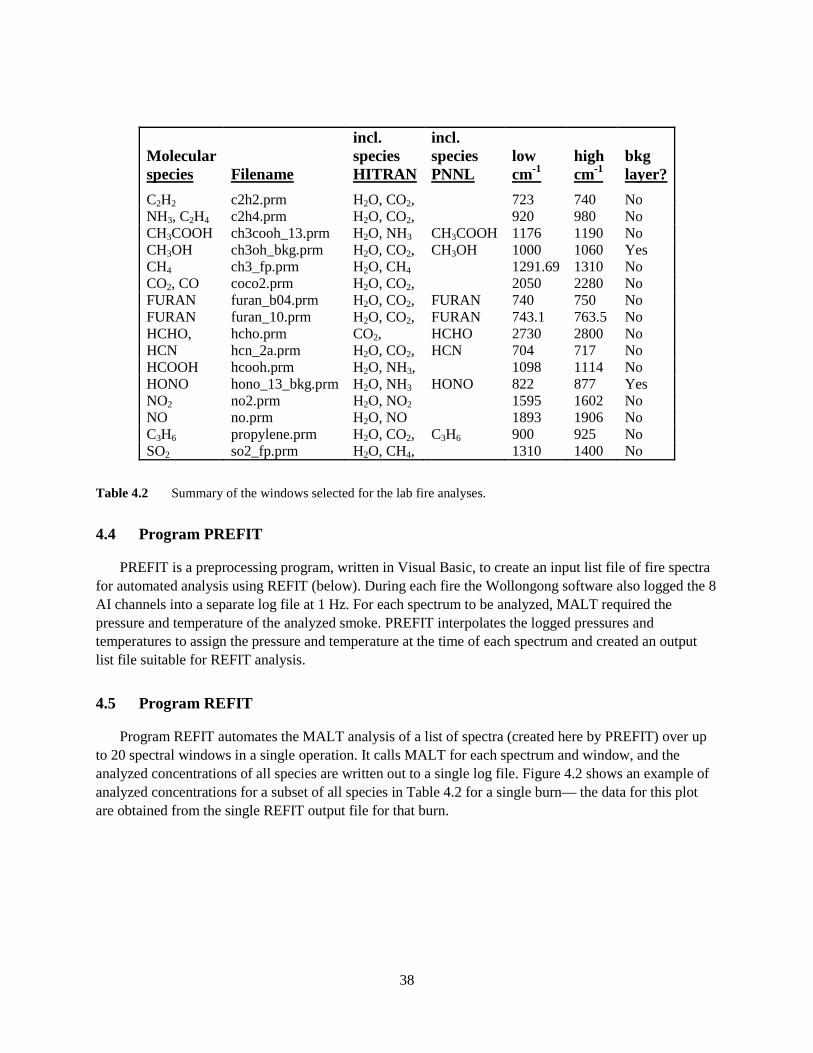
38
Molecular species Filename
incl. species HITRAN
incl. species PNNL
low cm-1
high cm-1
bkg layer?
C2H2 c2h2.prm H2O, CO2,
723 740 No NH3, C2H4 c2h4.prm H2O, CO2,
920 980 No
CH3COOH ch3cooh_13.prm H2O, NH3 CH3COOH 1176 1190 No CH3OH ch3oh_bkg.prm H2O, CO2,
CH3OH 1000 1060 Yes
CH4 ch3_fp.prm H2O, CH4 1291.69 1310 No CO2, CO coco2.prm H2O, CO2,
2050 2280 No
FURAN furan_b04.prm H2O, CO2,
FURAN 740 750 No FURAN furan_10.prm H2O, CO2,
FURAN 743.1 763.5 No
HCHO,
hcho.prm CO2,
HCHO 2730 2800 No HCN hcn_2a.prm H2O, CO2,
HCN 704 717 No
HCOOH hcooh.prm H2O, NH3,
1098 1114 No HONO hono_13_bkg.prm H2O, NH3 HONO 822 877 Yes NO2 no2.prm H2O, NO2 1595 1602 No NO no.prm H2O, NO 1893 1906 No C3H6 propylene.prm H2O, CO2,
C3H6 900 925 No
SO2 so2_fp.prm H2O, CH4,
1310 1400 No Table 4.2 Summary of the windows selected for the lab fire analyses.
4.4 Program PREFIT
PREFIT is a preprocessing program, written in Visual Basic, to create an input list file of fire spectra for automated analysis using REFIT (below). During each fire the Wollongong software also logged the 8 AI channels into a separate log file at 1 Hz. For each spectrum to be analyzed, MALT required the pressure and temperature of the analyzed smoke. PREFIT interpolates the logged pressures and temperatures to assign the pressure and temperature at the time of each spectrum and created an output list file suitable for REFIT analysis.
4.5 Program REFIT
Program REFIT automates the MALT analysis of a list of spectra (created here by PREFIT) over up to 20 spectral windows in a single operation. It calls MALT for each spectrum and window, and the analyzed concentrations of all species are written out to a single log file. Figure 4.2 shows an example of analyzed concentrations for a subset of all species in Table 4.2 for a single burn— the data for this plot are obtained from the single REFIT output file for that burn.

39
Figure 4.2 Example of time series of species measured by the FTIR during one fire using the software programs
PREFIT and REFIT.
4.6 Additional Improvements to MALT
During the SERDP 1649 project we made some critical improvements to MALT that accelerated and improved the accuracy of the smoke quantification measurements. These included:
1. Modifications to the MALT spectral model to account for differences between the pressure and temperature of the reference spectra (1013 hPa, 23ºC) and ambient conditions in the IFSL measured spectra (~900 hPa, 20-70ºC), and differences in the buffer gases (air v. N2).
2. Spectral regions were optimized for the analysis of each new target species.
3. New spectra of species generated in the PNNL library (Chapter 5) were imported into MALT.
4. All spectral analyses were incorporated into both online (real-time) and offline automated spectral analysis procedures to provide automated analysis of sets of spectra for all gases.
40
5.0 Chapter 5
Expanding the PNNL Infrared Spectral Database1
5.1 Introduction and Need for Expanded Database
As discussed in Chapters 3 and 4, one prerequisite to using the new dedicated IR spectrometer and the associated MALT software for analysis for the IR measurements is having at hand the IR reference spectra with which the laboratory and field data can be evaluated. Such reference spectra must be acquired in special laboratories using vetted procedures with exacting quality control. As part of the work we have therefore expanded the existing PNNL IR database of reference spectra to include more than 50 species associated with the DoD-prescribed burns. Detection of such species is thus enabled.
Originally, the PNNL infrared spectral library was created between 2000 and 2007 and was sponsored by the U.S. Department of Energy (DOE) for monitoring energy production gases as well as for homeland security applications [Johnson et al. 2002, Sharpe et al. 2004]. The data are for broadband sensors, either passive or active, that detect gas emissions associated with many types of energy production (coal, gas, nuclear) along with numerous environmental pollutants and toxic industrial chemicals (TICs). Three important characteristics of the spectroscopic data are: 1) they have a large spectral frequency range (minimum span of 600 to 6,500 cm-1); 2) the spectra are quantitative on the y-axis corresponding to 1.0 ppm-m at 1 atmosphere and 296 K; and 3) the spectral resolution is high, 0.11 cm-1, effectively the narrowest linewidths that would be encountered when monitoring near the earth’s surface due to the ~760 Torr pressure broadening. The database has applications beyond passive and active broadband monitoring: For example, since the data are quantitative, the integrated band strengths can be used to quantify absolute line intensities in high resolution low-pressure gas studies. The spectra are also useful for instructional purposes, e.g. in courses teaching spectroscopy.
Since any measurement is likely to involve a multitude of both biogenic (NH3, CO2, H2O, CH4) and anthropogenic (CO, SOx, NOy, freons, mineral acids…) interferents, the list of molecules contained in that DOE database had grown large (>400 compounds). However, one category of molecules that had not been specifically targeted in the DOE database was gases emitted by vegetation fires. While fire has been used for most of human history, biomass burning has only been studied by atmospheric chemists since ~1979 [Crutzen et al.], but interest has increased greatly since that time. Biomass burning includes landscape scale fires, but also small indoor fires used for cooking food that are a major atmospheric source due to their large numbers [Bertschi et al. 2003]. Recent estimates [Yokelson et al, 2008] of the total amount of biomass burned globally are approximately 5 to 7 Pg C/year. In the United States and other countries prescribed fire is used as land management tool (e.g. on military installations as discussed in Chapter 2 as well as on timber production lands) to manage hazardous fuels to minimize the impact of wildfires, and promote desirable stand characteristics; many stands are burned on a three- to four-year rotation. Thus, quantitative information was needed to study the impact of the trace gas and particle emissions on human health and atmospheric chemistry. 1 Some of the material in this chapter has already been reported as an open literature publication. Please see T.J. Johnson, L.T.M. Profeta, R.L. Sams, D.W.T. Griffith and R.J. Yokelson, 2010, “An Infrared Spectral Database for Detection of Gases Emitted by Biomass Burning,” Vibrational Spectroscopy, vol. 53, pp. 97-102,

41
Based on such considerations, an example of one class of compounds that warranted inclusion in the database is terpenes, hemi-terpenes, retenes, and related species: While isoprene was in the original PNNL database, we added several molecules such as limonene, the carenes, pinenes, pyrene, myrcene, etc. Along with isoprene, such unsaturated compounds are well known to be emitted directly by plants, but also produced by the heating of vegetation [Yokelson et al. 2008, Yokelson et al. 1996]. Related compounds whose IR spectra were included are oxidation products of these species, namely alcohols, aldehydes, ketones, and ethers. The oxidation of terpenes and hemi-terpenes (such as isoprene) is a dominant process known to create a wide variety of carbonyl compounds, some of which continue on to react with OH or further oxidize in the atmosphere [Finlayson-Pitts and Pitts, 2000]. Isoprene has a median concentration of up to ~2 ppbv in wooded areas of the southeastern U.S., and those levels rise as isoprene is released during biomass burning, thereby increasing the number of reactive carbonyl compounds subsequently created in the atmosphere. Specific examples of additional spectra that were needed include pentanal, glyoxal, methylglyoxal, diacetyl, 1-penten-3-ol, 2-pentanone, guaiacol, etc. The relevance of such compounds, including their role as potential precursors in the formation of secondary organic aerosols (SOA) was discussed for example by Yokelson et al. [2008] as well as in Pankow [1994].
5.2 Expanded List of Molecules
Based on the above considerations it was clear that while the DOE library contained hundreds of atmospheric species of common interest (e.g. H2O, SO2, NOx, freons, CH3OH), as well as some species known to be products of biomass burning such as alkenes, NH3, HCHO and CH3COOH, the IR database was not originally funded by DOE as a general tool for atmospheric chemistry nor biomass burning science. As a consequence, the parallel works of Profs. Griffith, Yokelson, and others had identified that many important burn-generated chemical species were not in the PNNL database that were needed to derive realistic EF for important fire-emitted gases. Many techniques have proven useful for quantifying the gases emitted by biomass burning (BB). Examples include whole air sampling in canisters followed by GC analysis for hydrocarbons and FTIR and mass spectrometry for on-line measurements of the hydrocarbons, other volatile organic compounds (VOC), and inorganic species [Yokelson et al., 2007]. These studies had shown that typically 60 to 80% of the non-methane organic compound (NMOC) emissions from biomass burning are in the form of the more reactive oxygenated VOC (OVOC). [Yokelson et al., 2008], most of which were not in the PNNL database.
Acquiring the reference spectra of such species at the state-of-the-art PNNL spectroscopy laboratory ultimately enabled this project to obtain fast, accurate IR measurements of those species. A first major task of the RC-1649 research project was therefore to augment the PNNL infrared library with the reference spectra of ~50 new species, with initial suggestions originally coming according to three main criteria:
1. Known initial burning emissions for which high-quality IR spectra are not available (e.g. acetol).
2. Known or suspected photochemical products of the initial burn-generated species, for example methyl vinyl ketone and methacrolein as oxidation products of isoprene.
3. HAPs that are regulated by the EPA and are suspected of being emitted by fires.
An example of a HAP addressed by criterion 3 includes vinyl phenol, which was detected in smoke by GC/MS techniques that are subject to severe interference problems. A preliminary search for vinyl

42
phenol in IR spectra of biomass burning smoke (using a generic reference spectrum) was negative [Christian et al., 2004], and this was therefore recognized as an example of the dearth of a needed spectrum.
We recognized, however, that many of the molecules found in BB plumes, however, already had spectra in the PNNL [Johnson et al., 2002], HITRAN [Rothman et al. 2009] or GEISA [Jacquinet-Husson et al. 2008] databases. For example, many common BB gases such as CO, CO2, H2O, NO and NO2 etc. are in most IR databases due to their ubiquitous occurrence in the atmosphere. Other species were already in the PNNL database due to their role as pollutants (e.g. SO2, H2SO4, HNO3 etc.) or as biogenic emissions that could interfere in the analysis of pollutants (e.g. isoprene, methacrolein, formaldehyde). It was estimated that 40 to 50 BB emission reference spectra already existed, and could be quantified by IR spectroscopy. But it was also anticipated that even more (particularly OVOCs) might be observed if reference spectra were available. The first step was to down-select from the above wish list and identify what compounds needed to be added to the database, the main criterion being that they are known or suspected BB emissions or smoke plume photochemistry products. Ultimately, by IR or other methods, it was necessary to derive as many emission factors (EF, that is, g emitted compound per kg dry biomass burned) for different types of fuels, conditions, etc. as possible.
Identification of actual candidates therefore relied on a literature search: To finalize the list, four concrete selection criteria were used: 1) The species had been seen in a BB plume by non-IR methods or was expected to occur based on known chemistry; 2) The species was expected to have reasonably strong IR absorption in the 1,300 to 700 cm-1 fingerprint region (e.g. species such as elemental Hg or CBr4 would be ruled out); 3) The species had a vapor pressure >~0.01 Torr or a boiling point of < 250 to 300 C, so that it was both amenable to laboratory measurement and would not immediately condense in a BB plume; 4) The species could be reactive in the atmosphere, but must have been sufficiently stable in an N2 bath gas in the lab (minutes to hours) so the measurement could actually be completed. The final list of proposed species is shown in Table 5.1, with the pink “x” behind the name indicating it was completed, i.e. its spectrum recorded and added to the spectral library.

43
Table 5.1 List of proposed compounds for IR spectra suggested as part of the biomass burning IR spectral
database. A pink “x” after the entry means it was completed.
5.3 Procedures and Methods
5.3.1 Acquisition Parameters and Objectives
The methodologies used to collect the data for this library have been previously described [Johnson et al., 2002, 2005 Sharpe et al. 2004, Foster et al. 2004]. Many of the salient features of the IR database are summarized in Table 5.2 below. The most important aspects are that the data are in fact quantitative, with each resultant spectrum derived from 10 or more individual quantitative measurements, the resolution is quite high, and that the data are carefully calibrated on both the wavelength and intensity axes.

44
Table 5.2 Experimental and Acquisition Parameters associated with the PNNL SERDP database of infrared
reference spectra.
5.4 Instrumental Methods
The spectrometers used were two Bruker IFS 66v/S vacuum benches; vacuum spectrometers eliminate spectral interference from H2O and CO2 lines and provide more intensity stability. We have documented all relevant parameters associated with both data acquisition and data processing in earlier papers; the reader is directed to these references for greater detail [Johnson et al., 2002, 2005 Sharpe et al. 2004, Foster et al. 2004]. Briefly, however, each system uses a glow bar source, a germanium on KBr beamsplitter, a mid-band photoconductive mercury cadmium telluride (MCT) detector, and a second aperture system (vide infra). For species of moderate to high volatility, a fixed 19.96 cm cell is used in the standard compartment and the vapor phase mixtures are generated by passive vaporization followed by filling with N2 ballast gas. For low volatility liquids whereby only small gas-phase mixing ratios can be achieved, a long-path White cell (set to 8.05 meters) is used to increase the path and an active disseminator is used to quantitatively and actively generate the gas mixtures [Johnson et al. 2006]. The disseminator dispenses the liquid at a fixed volume rate from a syringe pump onto a heated surface where it is flash vaporized on a stainless steel surface, and eluted with N2 gas from a calibrated mass flow controller. Photographs of the spectrometers and analyte handling systems can be seen in Figure 5.1.

45
Figure 5.1 Photographs of IFS 66v spectrometers and gas dissemination systems. The static system gas manifold
is at left, the active disseminator system at right.
We note that both the PNNL spectrometers were modified to redress two artifacts that give rise to photometric errors; both phenomena arise at the aperture [Johnson et al. 2002]. One of these is the “warm aperture” problem, [Johns, 1995] whereby at high resolution the cooled (MCT) detector sees not only source radiation through the aperture hole, but also the aperture annulus, which is near or above room temperature. The metal annulus therefore effectively serves as a warm blackbody source. These blackbody rays do not satisfy the resolution condition since they enter the interferometer as off-axis rays; the effect in spectral space is a distorted absorption line shape that shows a “tailing” to red frequencies. The second artifact [Johnson et al. 2002] is caused by light that has already been modulated by the interferometer returning toward the source and being reflected by the reflective polished metal surface on the back of the aperture (wheel) to re-enter the interferometer and be modulated again. This “double modulation” produces an optical 2f alias that can add spurious signals and distort intensities at all wavelengths. The PNNL spectrometers have both been modified to remove these two effects by adding a second focal plane with aperture after the interferometer that mimics the optical speed of the original system. The light seen by the detector from the back of the second aperture is not modulated, and as a DC signal is filtered away by the Fourier transform. To minimize well-known MCT nonlinearity problems we have used a software correction [Keens and Simon, 1990] from the spectrometer manufacturer that functions independent of the electronic bandwidth to compensate for the MCT’s nonlinear conversion of photons to signal, especially near the interferogram centerburst.
Because many of the analytes for the SERDP project were liquids, the experimental setup used to record their spectra is shown at right in Figure 5.1. Typically, 0.5 ml of the liquid was loaded into a gas-tight 500 microliter syringe and placed into the syringe pump. The syringe needle was inserted into the septum contained in the Swagelok tee. Single-channel background (I0) spectra were recorded while flowing only N2. Several different single-channel sample spectra (I) were recorded while the syringe pump liquid disseminator and mass flow system were both operating and stabilized. A minimum of 10 different concentrations were acquired by setting the syringe pump injection rate to various flow values. Spectral acquisition did not begin until a constant signal was observed on the real-time display of the FTIR. The flow rate was held at a stable value for the duration of each measurement. The gas flowed into a long-path White cell, where the IR beam interrogated the gas stream, absorbing at characteristic IR frequencies for each species. The wavelength axis was routinely calibrated using 165 individual rotational-vibrational lines of CO and N2O gases at low pressure to achieve a wavelength precision of better than 0.003 cm-1.

46
5.4.1 Data Collection and Data Processing
The PNNL data averaging scheme used a weighting mechanism that corrects for Beer’s law nonlinearity deviations. The absorbance was scaled to a calibrated value (1.0 ppm-m at 296 K, 1 atm) by using careful methods for measuring the optical pathlength, as well as periodic intensity calibrations using known absorbers, commonly isopropyl alcohol (2-propanol). In the PNNL data analysis method (Sharpe et al. 2004; Johnson et al. 2002), a composite spectrum was derived from a series of measurements, and in the series each spectrum corresponds to a different concentration-path length burden. In fact, each composite spectrum represents a series of >10 individual measurements at 298.1 K, with the different measurements covering a large range (often > 2 orders of magnitude) of analyte burdens, each burden pressurized with pure N2 to one atmosphere. An example of the concept, showing only 5 of the 17 actual measurements burdens is seen in Figure 5.2 for the species tetralin (1,2,3,4-tetrahydronaphthalene).
Figure 5.2 Infrared spectral curve of growth for tetralin displaying 5 of 17 acquired spectra.
The final fitted spectrum is in fact derived by fitting a Beer’s Law plot at each wavelength channel to the individual burdens. To account for any of several different nonlinearity phenomena in the A = f(P) fit, the individual burdens were, in addition, weighted according to T2 (where T = I/Io). All values with T < 0.025 (i.e., absorbance A > 1.6) were simply weighted with zero in the fit. This multiple burden with weighted data approach retains several advantages over any single measurement or few measurements: First, multiple measurements greatly enhance the signal-to-noise ratio (SNR). Second, the high burden measurements enhance the SNR for the weak bands that might not exceed the noise floor in any measurement designed to keep the strong bands on scale. Third, for the strong bands, the weighting mechanism brings out better fidelity to account for Beer’s Law saturation effects, detector nonlinearity effects, or other phenomena that cause nonlinear results. The fitting process was applied to the data such as those graphically displayed in Figure 5.2. The slope of the fitted line at any given wavelength channel gave the value for the absorption coefficient at this spectral position. The slope at each spectral bin was computed for all spectral bins, resulting in the absorption coefficient vector (spectrum). The composite spectrum was then converted to units of (ppm)-1m-1 and normalized for a gas number density corresponding to 296 K, assuming ideal gas behavior (PV = nRT).

47
5.4.2 Examples of SERDP-PNNL Infrared Data
Table 5.1 also summarizes the current status of the biomass burning infrared database in terms of those species completed through December 2012. This includes whether the species were measured using the static system with passive evaporation or the flow system with the active disseminator. As discussed below, all measured IR spectra are digitally available at nwir.pnl.gov, including the metadata associated with each file. The associated metadata files also indicate whether the data were recorded on either of two systems, with the lower volatility samples being reserved for the flow disseminator – white cell system. Extensive other data about the sample and spectroscopy are also found in the metadata files.
While this report will not discuss all the results, Figure 5.3 presents a typical result of the IR spectrum for a gas species associated with burning effluents, namely the quantitative broadband IR spectrum of 3-methyl-1-butanal (a.k.a. isovaleraldehyde). Isovaleraldehyde is a flavoring agent and occurs naturally in oils (lavender, peppermint) as well as coffee extract. It is also suspected to be in biomass burning plumes as it has been observed as a (photo-) oxidation product of isoprene and other terpenes via methacrolein [Duane et al. 2002, Liu et al. 2009]. The spectrum is seen to contain multiple bands in the longwave infrared (LWIR), as well as the C-H stretching region (midwave IR) that can all be used for identification.
Figure 5.3 Composite 298 K infrared spectrum of isovaleraldehyde from 10 individual measurements. The y-axis
is quantitative and corresponds to an optical depth of 1 ppm-meter
As is typical of ketones and aldehydes, [Socrates 1994] the most intense band in the spectrum arises from the carbonyl stretching frequency in the ~1730 cm-1 domain, in this case 1746.1 cm-1 for isovaleraldehyde. For atmospheric remote sensing applications, however, such bands are sometimes of limited utility due to interference from the ro-vibrational lines of the water ν2 bending mode. However, the spectrum is seen to contain multiple relatively strong bands in the longwave infrared, as well as the C-H stretching region (midwave IR) that can all be used for identification. As is typical for hydrocarbons and moderately substituted hydrocarbons, the C-H stretching region provides many strong bands in the 2,800 to 3,100 cm-1 domain. While such broad C-H bands can provide good sensitivity and can thus be useful for gas-phase monitoring, in the absence of any rotational structure they provide little specificity: Essentially every hydrocarbon, including most substituted species, has the typical broad C-H stretching features at these wavelengths, though for isovaleraldehyde the peak at 2967.37 cm-1 is sharp (pseudo Q-branch width ~2.9 cm-1) providing some specificity. Of greater utility, however, is the sharp doublet at 2712.7 and 2704.3 cm-1. This is a somewhat unusual region for such a strong absorption; it corresponds to one of the two fundamental C-H stretching modes involving the aldehyde carbon, and this mode is in Fermi resonance with the first overtone of the C-H bending vibration [Silverstein and Webster 1998]. The other aldehyde C-H stretching mode occurs at a characteristic value of 2818.16 cm-1 [Socrates 1994]. The 2712 and 2704 peaks occur at frequencies low enough to avoid interference from the water O-H

48
stretching modes, but at frequencies greater than the R-branch lines of the CO2 ν3 asymmetric stretch in the 2350 cm-1 region.
As an example of a different class of compounds, Figure 5.4 presents a typical result for the broadband IR spectrum of 2-vinylpyridine (also known as α-vinylpyridine). In terms of sources, 2-vinylpyridine known primarily as an industrial compound, mostly used in tire manufacturing as a tire cord and belt additive. It is also a known component of tobacco smoke [Eatough et al. 1989] and is thus suspected to be emitted in biomass burning. Its reactions with the common atmospheric oxidants either O3 or the OH radical are known to produce 2-pyridinecaboxaldehyde and formaldehyde [Tuazon et al. 1993]. The IR spectrum contain multiple strong bands in the longwave infrared between 700 and 1,300 cm-1, and many of these bands (or all in combination) are well suited for atmospheric monitoring.
Figure 5.4 Composite 298 K infrared spectrum of 2-vinylpyridine from 11 separate measurements. The y-axis is
quantitative and corresponds to an optical depth of 1 ppm-meter.
The 2-vinylpyridine spectrum is seen to contain multiple longwave IR bands, as well as in the midwave infrared C-H stretching region, all of which can all be used for identification. One feature of the vinyl pyridine spectrum of note, however, is common to dozens of species in the PNNL gas-phase database, especially for the aromatic molecules, namely that the compound has (multiple) very sharp Q-branches, often associated with ring or conjugated bond modes. These are seen in the inset of Figure 5.4. While 2-vinylpyridine is of no or low symmetry (Cs point group due to the mirror symmetry in the plane of the molecule, assuming no free torsion motion about the ring-vinyl C-C bond), the spectrum still exhibits several very sharp, well-resolved Q-branches. For example, the peaks at 938.93 cm-1 and 741.20 cm-1 exhibit Q-branch linewidths of only 0.72 and 0.68 cm-1 FWHM, respectively. Such peaks are clearly useful for broadband (FT) infrared monitoring. Equally important, such sharp Q-branches are especially amenable to infrared laser monitoring. External cavity quantum cascade lasers (QCLs) can now tune in frequency upwards of 200 cm-1. Even without external cavity tuning, modern QCLs can readily tune 5 cm-1 by varying the temperature or current [Taubman et al. 2004]. This implies that modern IR laser systems together with the observed sharp features can provide ultrasensitive (ppt-level) detection of such species even in open path systems with the species pressure-broadened to atmospheric pressure. Due to the intrinsically sharp absorption lines, the resulting specificity is very high, and due to the inherent brightness of the lasers systems (vis-à-vis thermal sources) the sensitivity can be orders of magnitude higher, though only over a limited spectral range. Because such systems could be constructed as open-path systems, greater path lengths could be achieved without extractive degradation of the compounds.

49
5.5 Updating and Disseminating the IR Reference Database
PNNL continues to deliver its spectral database of broadband infrared reference spectra that has been expanded to include spectra of those gas-phase species associated with biomass burning. Table 5.1 contains those species that were measured and as part of the PNNL SERDP infrared database. The table does not include the many dozens of biomass burning gases that are already included in the PNNL reference database such as alkanes, alkenes, aromatics; MVK, etc. The complete contents of both databases can be found at https:\\nwir.pnl.gov. This web site is maintained by PNNL and the data are free to the public.
5.6 Demonstrated Utility of New Reference Spectra
During the course of the project approximately 55 new species were continually added to the IR database. As will be discussed in Chapters 6 to 10, unassigned absorption features can nevertheless remain in the residual spectra after performing MALT analysis on spectra collected from biomass burning smoke. For example, Yokelson et al. [1996] and Burling et al. [2011] noted large, IR spectral features in smoke similar to C10 absorption, suggesting possible large emissions of monoterpenes. Using the newly added, optimized limonene spectral window, we reported the first quantitative FTIR observations of a monoterpene (limonene) in smoke from field fires in 2011 [Burling et al. 2011]. Limonene is a dominant monoterpene that is especially susceptible to oxidation, providing a quick, direct route to forming low-vapor pressure oxidation products that are likely to form a disproportionate amount of secondary organic aerosol (SOA) relative to other monoterpenes [Lane et al., 2008; Maksymuik et al., 2009; Fry et al., 2011]. As seen in Figure 5.5 the sample of smoke from the smoldering base of a damaged, live tree was characterized by much higher hydrocarbon emissions than the dead stump samples, including very high isoprene and 1,3‑butadiene emissions even though it burned with the highest MCE of samples at this site. For illustration purposes, a reference spectrum for the figure (dark blue trace in Figure 5.5) was composed by adding equal mixing ratios of the three terpene species α–pinene, β-pinene and D-limonene.

50
Figure 5.5 Absorption spectra of ground samples normalized to the CO absorption band centered at 2143 cm-1.
Samples s1-s3 are of smoldering emissions from dead stumps while samples s5 is combustion occurring at the base of a living tree. The blue reference spectrum is a linear sum of 3 equal parts of reference spectra of the monoterpene species α-pinene, β-pinene, and D-limonene.
In addition to limonene, we measured several other compounds in the field that had been recently added to the PNNL spectral database, including phenol, 2-methylfuran, glyoxal, and glycolaldehyde. Glycolaldehyde (GA, 2-hydroxyethanal, C2H4O2) is a semi-volatile molecule of atmospheric importance, recently proposed as a precursor in the formation of aqueous-phase secondary organic aerosol [Pankow, 1994]. Extensive work was performed to identify the unknown species that are notoriously difficult to measure. For example, glycolaldehyde is difficult to measure mainly due to interferences in mass spectrometry (mass 60), its “sticky” behavior in gas chromatography, and its propensity to both dimerize and condense. Infrared spectroscopy has been used occasionally over the past 30 years to measured GA, although our literature search suggested that there were few atmospheric measurements and vibrational assignments for GA were incomplete or unsatisfactory. The IR cross-sections used in previous works [Yokelson et al., 1997; Bertschi et al., 2003; Christian et al., 2004] were later shown to be incorrect via comparison to our new reference spectrum. Thus recognizing the importance of this reactive organic molecule, we tried to better assess its source term as derived for biomass burning, particularly for fuel types and ecosystems not previously studied.
Using the vetted protocols described above we not only measured its quantitative spectrum, but also completed the first assignment of all fundamental vibrational modes and derived quantitative IR absorption band strengths using both neat and pressure-broadened GA vapor. [Johnson et al., 2013]. Our derived intensities agreed well with the few previously published values. More importantly, using the reference ν10 band Q-branch at 860.51 cm-1, we determined GA mixing ratios in biomass burning plumes generated by both the field and laboratory burns of fuels from the southeastern and southwestern U.S., including the first field measurements of glycolaldehyde in smoke. As seen in the example of Figure 5.6, the reference spectra of glycolaldehyde (GA), NH3, H2O, and HONO were used to fit smoke spectra in the region of the GA ν10 band near 861 cm-1. The displayed smoke spectrum was acquired from an

51
airborne FTIR smoke sample from a prescribed burn at Vandenberg Air Force Base, California on 5 November 2009. The GA reference spectrum is in blue with upward-facing peaks. The upper two traces (downward peaks) represent the experimental spectrum (red) and fit thereto (blue) with the residual (measured minus fitted) shown as the top trace.
Figure 5.6 The reference spectra of glycolaldehyde, along with NH3, H2O, and HONO were used to fit smoke
spectra in the region of the GA ν10 band near 861 cm-1. The smoke spectra were acquired from a prescribed burn at Vandenberg Air Force Base, California on 5 November 2009. The GA reference spectrum is in blue with upward-facing peaks. The upper two traces (downward peaks) represent the experimental spectrum (red) and fit thereto (blue) with the residual (measured minus fitted) shown as the top trace.
In that study, the GA emission factors were anti-correlated with modified combustion efficiency, thus confirming release of GA from smoldering combustion. The GA emission factors (g of GA emitted per kg dry biomass burned on a dry mass basis) had a low dependence on fuel type consistent with the production mechanism being pyrolysis of cellulose. GA was emitted at 0.23 ± 0.13% of CO from field fires and we calculated that it accounted for ~18% of the aqueous-phase SOA precursors that we were able to measure.
While there are several more examples, this section of the report has documented two clear-cut cases where it was only the availability of the reference spectra in the PNNL database that made discovery of such species possible in the biomass burning plumes. Spectral analysis continues to look for more such cases in our field spectra.

52
6.0 Chapter 6
Laboratory Experiments at the Fire Sciences Laboratory (FSL) in Missoula Montana.2
6.1 Introduction and Motivation for Laboratory Studies
As outlined in the introduction, most DoD bases are in ecosystems that co-evolved with fire as a major natural influence. Removing fire from these ecosystems causes an unnatural buildup of fuels that increases the severity of wildfires, threatens endangered species, and can severely limit DoD training objectives. Thus, carefully planned prescribed fires (PF) have become a vital land management tool for DoD (e.g. bases in pine savanna often burn the understory on a ~three year cycle). However, as population increases near the bases, so does the potential that smoke from a prescribed fire might cause undesired air quality impacts for local or regional residents. Moreover, some bases are in areas that are already near non-compliance with federal standards for ozone and fine particles (PM2.5) even before PF are considered. Responsibility for protecting air quality lies mostly with state-level smoke management authorities who ultimately approve or disallow PF. The smoke management team considers the requested burn location and size and combines that with their best estimates of the fuel consumption (FC, mass of fuel burned per unit area), emission factors (EF, mass of pollutant emitted per mass of fuel burned), and smoke dispersion (based on expected injection altitude and forecast winds). A major problem in the whole permitting/PF cycle, however, is that all the necessary estimates are highly uncertain. This is especially true for DoD PF for which there are few measurements of any of the above parameters.
In terms of results of greatest relevance to be directly used by DoD and various smoke management authorities, the main deliverables of SERDP project RC-1649 (in conjunction with RC-1647 and RC-1648) were generated in the three intensive observation periods (IOPs) in both the laboratory and field experiments. The first of these was an experiment for measuring EF for simulated DoD fires in the USFS large-scale combustion lab using a powerful array of atmospheric chemistry instruments. Specifically, an array of fuels were collected from DoD sites in the southeastern and southwestern U.S. during early 2009 and were burned at the Missoula Fire Sciences Laboratory (FSL) and burned in a series of 77 fires during February and March of 2009.
While field measurements are essential to characterize smoke from real fires, laboratory studies such as those described in this chapter offer many advantages [Yokelson et al., 2008]. More extensive instrumentation can be utilized in laboratory fire studies—and since smoke concentrations tend to be
2 Much of the material in this chapter has already been reported as an open literature publication. Please see “Laboratory measurements of trace gas emissions from biomass burning of fuel types from the southeastern and southwestern United States,” by Burling, I. R., Yokelson, R. J., Griffith, D.W.T., Johnson, T. J., Veres, P., Roberts, J.M., Warneke, C., Urbanski, S.P., Reardon, J., Weise, D.R., Hao, W.M., and de Gouw, J.:, Atmos. Chem. Phys., 10, 11115-11130, doi:10.5194/acp-10-11115-2010, (2010). We also acknowledge contributions from Patrick Veres, James M. Roberts, Carsten Warneke and Joost de Gouw of NOAA, Shawn P. Urbanski and James Reardon of the U.S Forest Service for these experiments and results. We appreciate the efforts of Joey Chong, Bonni Corcoran, Amy Olson, Violet Holly, Signe Leirfallom, and Emily Lincoln to harvest the fuels and assemble the fuel beds for this study. The cooperation of Dan Ardoin and personnel at Vandenberg AFB, Jeff Minetti and personnel at Fort Hunter-Liggett, Andrew Leiendecker and personnel at Fort Huachuca, and Danny Becker, Susan Cohen, Wayne Gray at Camp Lejeune as well as Gary Curcio (NC Forest Service) is greatly appreciated.

53
higher, more species can be quantified. Also, in a laboratory experiment, all the smoke during the entire course of a fire can be sampled, so that emission factors can be determined with high accuracy, whereas field measurements are typically limited to sampling a much smaller fraction of the total smoke (see following chapter). Characterization and measurement of the composition of fuels and the conditions under which they are burned is easier in the laboratory. In the laboratory component described here, fuels representative of vegetation commonly managed by prescribed burning on several southeastern and southwestern DoD bases were collected and burned under controlled conditions at the U.S. Forest Service (USFS) Fire Sciences Laboratory in Missoula, Montana. The emissions from these laboratory burns were analyzed with a large suite of state-of-the-art instrumentation. The data from these controlled laboratory burns were synthesized with data from actual field measurements (both airborne and ground-based) of prescribed burns of the same fuels on DoD bases. The objective of the present study was to derive emission factors of the gas-phase species measured by OP-FTIR in the laboratory.
During each fire, we measured the smoke (and fuel) composition with a comprehensive suite of advanced instrumentation from SERDP projects as well as multiple collaborators. Measurements included: filter sampling of particles by numerous complementary collection techniques. This was followed by analyses of metals, ions, and elemental and organic carbon; real-time particle chemistry by aerosol mass spectrometer, particles-into-liquid samplers, and electrospray mass spectrometry; particle size distribution (including ultrafine nanoparticles); concentration by numerous complementary techniques; and trace gas analysis by open-path FTIR and other techniques.
During these experiments the smoke emissions were measured primarily an open-path Fourier transform infrared (OP-FTIR) spectrometer for measurement of gas-phase species. The OP-FTIR detected and quantified 19 gas-phase species in these fires: CO2, CO, CH4, C2H2, C2H4, C3H6, HCHO, HCOOH, CH3OH, CH3COOH, furan, H2O, NO, NO2, HONO, NH3, HCN, HCl, and SO2. Emission factors for these species are presented for each vegetation type burned. The lab fire results are already stratified into EF by fuel type (i.e. one-year rough, pocosin, etc.) and the same will be done for the final recommended EF.
There were several interesting results as described below, but two observations of particular note were that 1) both OP-FTIR and the NI-PT-CIMS observed significant amounts of nitrous acid (HONO) and were in excellent agreement with each other. The HONO was emitted during the flaming phase and was critical to smoke chemistry as it is a precursor for rapid formation of OH, which is the main species that removes pollutants from the atmosphere. Gas-phase HONO was detected in the smoke from all fires; the HONO emission factors ranged from 0.15 to 0.60 g kg-1 and were higher for the southeastern U.S. fuels. The fire-integrated molar emission ratios of HONO (relative to NOx) ranged from approximately 0.03 to 0.20, with higher values also observed for the southeastern U.S. fuels. Also, 2) The OP-FTIR system observed unusually elevated concentrations of hydrochloric acid (HCl) and SO2 from multiple fuels. Twenty-two, previously-unmeasureable organic acids were detected in the fire smoke and over 300 VOC were detected by the NOAA GC-MS. The majority of non-methane organic compound (NMOC) emissions detected by OP-FTIR were oxygenated volatile organic compounds (OVOCs) with the total identified OVOC emissions constituting 61±12% of the total measured NMOC on a molar basis. These OVOC may undergo photolysis or further oxidation contributing to ozone formation. Elevated amounts of gas-phase HCl and SO2 were also detected during flaming combustion, with the amounts varying greatly depending on location and vegetation type, the highest HCl emission factors were all located in the coastal regions, although HCl was also observed from fuels farther inland. HCl emission factors were

54
generally higher for the southwestern fuels, particularly those found in the chaparral biome in the coastal regions of California. These results are detailed below.
The relationship between EF and MCE for species measured in the same fuel types in the field will be compared to the lab relationship. If the equations are similar then we will use the lab-fire-based equations for species measured only in the lab to calculate the recommended EF for the species at the field-average MCE. If the equations are not similar, alternate methods of using lab data to derive EF appropriate for field fires have been described by Yokelson and other workers.
6.2 Fire Sciences Laboratory Combustion Facility
The layout of the combustion facility at the FSL is shown in Figure 6.1 and has been described in significant detail elsewhere [Christian et al., 2003]. Briefly, the combustion facility is a large chamber measuring 12.5 m × 12.5 m × 22 m high. As seen in Figure 6.1, a 1.6 m diameter exhaust stack with a 3.6 m diameter inverted funnel opening extends from ~2 m above the floor to the top of the chamber. Outside air is conditioned for temperature and relative humidity and slightly pressurizes the combustion chamber. This air is vented through the stack and entrains the emissions from fires burning directly beneath the funnel. A large sampling platform supporting the OP-FTIR and the majority of the instrumentation surrounds the stack 17 m above the fuel bed. Temperature and mixing ratios are constant across the width of the stack at the height of the sampling platform [Christian et al., 2003; Christian et al., 2004], providing a well-mixed sample. The fuel bed consisted of an aluminum frame with a wire grid.
Figure 6.1 Schematic of the Fire Lab and photo of a simulation fire in progress. The fires were
videotaped/archived for future fire behavior reference.
6.3 Fuel Descriptions, Collections and Laboratory Setup
Team member Jim Reardon (who is a USFS wildland fuels expert) met with SERDP representative Susan Cohen, base forester Danny Becker, and the DCERP team in the spring of 2008. Also during 2008, Reardon and Becker identified numerous sites that were scheduled to be treated with prescribed fire at

55
Camp Lejeune and Fort Benning during the spring 2010 field campaign. As described in the next chapter, Camp Lejeune burned mostly areas that have been “masticated” (i.e. mechanically chipped) followed by one or two years of re-growth before burning. This re-growth is commonly referred to as “one or two year rough.” Therefore, USFS crew that was hired, trained, paid, and led by Jim Reardon sampled the total fuel loading on numerous examples of one and two year rough and a few wetland (Pocosin) sites. This occurred during November 2008 and was documented with a CD of digital photographs. During January of 2009, fuels were collected from each site at Camp Lejeune and Fort Benning and shipped to Montana where they were dried and weighed by component (e.g. leaves, twigs, branches by diameter class, etc.). The “fuel loading” as a function of each fuel component’s characteristic “time-lag class” (essentially the drying rate) was also completed in early 2009. As part of our collaboration with RC-1648, D. Weise et al. perfected their fuel sampling technique for southwestern fuels and tested their framework for reconstructing realistic fuel beds. Weise et al. sent the same personnel that sampled the fuels at the Southwest sites to Missoula to rebuild the beds and ignite the fires for the smoke measurements. The southeastern U.S. fuels were also reconstructed by the sampling personnel; the fire constructing crew was experienced with southeastern U.S. forestry but also had the CD of photos as an aid. All the fuels burned in each lab fire were sub-sampled and analyzed for moisture content as well as C, H, N, S, and Cl content. The measurement of actual fuel consumption during the actual PF was carried out in concert with the spring 2010 field EF measurements (detailed in the following chapters).
Samples representing fuels commonly managed by prescribed burning were collected in January 2009 from Camp Lejeune, North Carolina. and Fort Benning, Georgia in the southeastern U.S., and Fort Hunter-Liggett, California, Vandenberg Air Force Base California, and Fort Huachuca, Arizona in the southwestern U.S. The species composition and other details of the samples burned in this study are listed in Table 6.1. We briefly describe the fuels here starting with the Southeast. Pocosin (fuel code in tables and figures is “poc”) is a dense shrub/pine complex that is extremely flammable during drought (Wendel et al, 1962). The pocosin site was a mix of fetterbush (Lyonia lucida) and gallberry (Ilex glabra). The understory hardwood (“uh”) samples were mostly understory red (Persea borbonia) and loblolly bays (Gordonia lasianthus) and some red maple (Acer rubrum). Some of the samples from Camp Lejeune represented different stages after mechanical fuel treatment and/or burning at that location. The chipped understory hardwood (“cuh”) samples were mostly larger diameter red maple, red bay and loblolly bay that had been recently mechanically masticated. Our samples were of the smaller diameter pieces (less than ~5 cm) of various lengths (up to ~30 cm) as these are the components that were most likely to burn in a prescribed fire. The “one-year rough” (“1yr”) and “two-year rough” (“2yr”) samples refer to understory regrowth one and two years after burning and they were dominated by a mix of gallberry, fetterbush and graminoids (grasses). The Fort Benning samples (“lit”) were litter from various aged stands of the four major southern pine species (longleaf, loblolly, shortleaf (Pinus echinata), and slash (P. elliottii).

56
Table 6.1 Summary of vegetation burned and fuel elemental analysis.
The southwestern samples from California were of six types of the dense, evergreen chaparral shrub complex common in much of California. The various types are shown in Table 6.1 along with their fuel codes. Chaparral covers roughly 2.5 million hectares and is known for its intense crown fires, which can impact urban areas [Keeley and Davis, 2007]. The Fort Huachuca samples from Arizona were from plant communities of the Sonoran Desert and the Madrean archipelago (sky islands) and consisted of masticated mesquite (Prosopis velutina) and desert broom (Baccharis sarothroides) (“mes”), oak savanna (Emory oak (Quercus emoryi) and Lehmann lovegrass, (Eragrostis lehmanniana) “oas”), and oak woodland (Emory oak and pointleaf manzanita (Arctostaphylos pungens), “oaw”). We also burned additional samples including a duff sample (“duf”) from a black spruce (Picea mariana) forest in Alaska , as well as Englemann spruce (“spr,” Picea engelmannii) branches, and ponderosa pine (Pinus ponderosa) needles (“ppn”) from Montana.
After collection, the fuel samples were sent to the FSL and stored for three to four weeks before burning in the laboratory. The fuel samples were re-assembled in the combustion chamber based on site photographs and fuel loading measurements. With the exception of the pine litter, masticated mesquite, and chipped understory hardwood fuel types, these fuels tend to have a vertical orientation in the natural setting where wind and slope often improve heat transfer and fire propagation. We initially attempted to burn the southwestern fuels in this orientation, but had limited success so the remaining southwestern fuels were oriented horizontally while maintaining a realistic mass per area so that the fire carried better. Nearly all of the fires were ignited with a propane torch. Data points corresponding to ignition were omitted from the analysis. All burns were filmed to enable subsequent re-examination of the fire behavior. The carbon and nitrogen content of the fuels were measured by the University of Idaho; Analytical Sciences Laboratory and fuel content results are shown in the right-most columns of Table 6.1. Oven-dry mass and fuel consumption data for the southwestern fuel types are reported in [Hosseini et al, 2010]. The oven-dry mass and fuel moisture data for the southeastern fuel types can be found in Table 6.2. Fuel bed properties for southeastern fuel types burned in laboratory experiment. Some fuel beds

57
were extinguished after sufficient data had been collected to produce consistent emission factors but before the fuel bed self-extinguished. This affects the consumption amount that is presented in Table 6.2. The table is based on the remaining mass when the burn was put out. Attempting to correlate consumption with fuel moisture for these data should not be done. The loading for the 1 and 2 year rough fuel types compares well with published loadings for 1 and 2 year roughs under longleaf pine [Ottmar and Vihnanek, 2000]. The pocosin loading compares favorably with loading for high pocosin and high brush fuel types [Ottmar and Vihnanek, 2000; Wendel et al 1962] as does the understory hardwood fuel type. Loading for the chipped understory hardwood fuel type is similar to that reported by Glitzenstein et al [2006] depending on which 10 hr fuel loading is used and within the range of the experimental fuel beds used by Kreye et al [2013].
Fuel code Mass (g) σ Moisture content (%) σ Consumption
(%) Loading
(tons/acre) 1yr 666 49 21.7 6.2 92 3.0 2yr 723 120 25.4 6.6 82 3.2 cuh 2672 382 5.6 1.5 95 11.9 uh 2019 702 12.4 10.7 65 9.0 poc 4627 505 12.1 9.1 58 20.7 lit 1180 253 4.6 1.4 72 5.3
Table 6.2. Fuel bed properties for southeastern fuel types burned in laboratory experiment.
6.4 Open-path Fourier Transform Infrared Spectrometer Details
The most useful technique for the measurement of gas-phase emissions from biomass burning in those experiments was an open-path Fourier transform infrared (OP-FTIR) spectroscopy as described in previous chapters. An advantage of OP-FTIR is that it is able to quantify most reactive and stable compounds at mixing ratios at or above a few ppbv. In addition, the open-path nature of the measurement produces no sampling or storage artifacts, and all compounds are measured simultaneously and path-integrated through the same air parcel. The unique spectral features of the species measured means the technique is resistant to interference and provides unambiguous compound identification. Also, OP-FTIR provides high temporal resolution for monitoring of dynamic processes related to emissions of biomass fires [Yokelson et al., 1996].
The open-path Fourier transform infrared (OP-FTIR) instrument consisted of a Bruker Matrix-M IR Cube spectrometer and a thermally stabilized open-path White cell. The 58.0 m path length White cell was positioned on the sampling platform approximately 17 m above the fuel bed so that the open path spanned the full diameter of the stack directly in the rising emissions stream. We performed several tests to determine the best spectrometer sampling options, including measurement duty cycle, sample frequency, and spectral resolution. Ultimately, spectra were acquired every 1.5 seconds (four co-added interferograms in 1.5 seconds, with duty cycle > 95%) at a spectral resolution of 0.67 cm-1 beginning several minutes prior to the fire and continuously until the end of the fire. A pressure transducer and two temperature sensors were located adjacent to the optical path and their outputs were logged on the computer and used for spectral analysis.
58
The acquired IR spectra were analyzed for carbon dioxide (CO2), carbon monoxide (CO), methane (CH4), ethyne (C2H2), ethene (C2H4), propene (C3H6), formaldehyde (HCHO), formic acid (HCOOH), methanol (CH3OH), acetic acid (CH3COOH), furan (C4H4O), water (H2O), nitric oxide (NO), nitrogen dioxide (NO2), nitrous acid (HONO), ammonia (NH3), hydrogen cyanide (HCN), hydrogen chloride (HCl), and sulfur dioxide (SO2). Mixing ratios were obtained by multi-component fits to selected sections of the mid-IR transmission spectra with a synthetic calibration non-linear least-squares method [Griffith, 1996; Yokelson et al., 2007a] utilizing both the HITRAN [Rothman et al., 2009] spectral database and reference spectra recorded at Pacific Northwest National Laboratory (PNNL) [Sharpe et al., 2004; Johnson et al., 2006; Johnson et al., 2010]. The species above accounted for nearly all the features observed in the smoke spectra. A comparison of our experimental smoke spectra to published reference spectra confirmed that several compounds that have been detected in past smoke studies by FTIR, such as ethane, glycolaldehyde, carbonyl sulfide, isoprene, and 1-butene were not present in detectable quantities.
6.5 Additional Instrumentation Details
In addition to the OP-FTIR, gas-phase measurements were also performed by (1) two proton-transfer-reaction mass spectrometers (PTR-MS) for measurement of non-methane organic compounds (NMOC) [de Gouw and Warneke, 2007], (2) proton-transfer ion trap-mass spectrometry (PIT-MS) [Warneke et al., 2005] for NMOC, (3) negative-ion proton-transfer chemical-ionization mass spectrometry (NI-PT-CIMS) [Veres et al., 2008] for detection of organic and inorganic acids, (4) gas chromatography mass spectrometry (GC-MS) for NMOC [Goldan et al., 2004], (5) canister sampling followed with analysis by gas chromatography flame ionization detection (GC-FID) [Hao et al., 1996] for low molecular weight hydrocarbons, (6) LICOR CO2 analyzer, and (7) TECO CO analyzer. Due to platform space and load restrictions, one PTR-MS and the GC-MS were housed in a control room adjacent to the combustion chamber and connected to the stack by a long Teflon sampling line. Together these additional instruments provided measurements of approximately one hundred additional trace gases. To characterize the particle emissions, several instruments located on the platform measured size distributions, number, mass, and composition. Full descriptions and results from the other individual instruments are published elsewhere [Hosseini et al., 2013; Roberts et al., 2010; Veres et al., 2010; Warneke et al., 2011].
During each fire, we measured the smoke (and fuel) composition with the most comprehensive suite of advanced instrumentation ever deployed in an atmospheric chemistry project (Table 6.3). The massive scale of this effort was made possible by collaboration with the two other SI projects (RC-1648 focused on southwestern fuels and RC-1647 focused on the fuels from Fort Benning); participation of a large team from NOAA that was funded by NSF; and no-cost contributions from NIOSH, PNNL and others. The measurements included: filter sampling of particles by numerous complementary collection techniques followed by analyses of metals, ions, and elemental and organic carbon; real-time particle chemistry by aerosol mass spectrometry, particle-into-liquid samplers, and electrospray mass spectrometry, particle size distribution (including ultrafine nanoparticles) and concentration by numerous complementary techniques; and trace gas analysis by our SERDP-funded, specially-built, open-path FTIR, a newly-invented negative ion proton transfer chemical ionization mass spectrometer (NI-PT-CIMS), the only existing PIT-MS, as well as GC, GC-MS, PTR-MS, and NDIR (See Table 6.3).
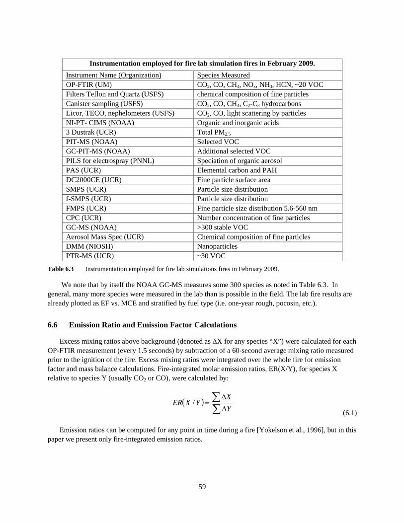
59
Table 6.3 Instrumentation employed for fire lab simulations fires in February 2009.
We note that by itself the NOAA GC-MS measures some 300 species as noted in Table 6.3. In general, many more species were measured in the lab than is possible in the field. The lab fire results are already plotted as EF vs. MCE and stratified by fuel type (i.e. one-year rough, pocosin, etc.).
6.6 Emission Ratio and Emission Factor Calculations
Excess mixing ratios above background (denoted as ΔX for any species “X”) were calculated for each OP-FTIR measurement (every 1.5 seconds) by subtraction of a 60-second average mixing ratio measured prior to the ignition of the fire. Excess mixing ratios were integrated over the whole fire for emission factor and mass balance calculations. Fire-integrated molar emission ratios, ER(X/Y), for species X relative to species Y (usually CO2 or CO), were calculated by:
(6.1)
Emission ratios can be computed for any point in time during a fire [Yokelson et al., 1996], but in this paper we present only fire-integrated emission ratios.
( )∑∑
∆
∆=
YX
YXER /
Instrumentation employed for fire lab simulation fires in February 2009. Instrument Name (Organization) Species Measured OP-FTIR (UM) CO2, CO, CH4, NOx, NH3, HCN, ~20 VOC Filters Teflon and Quartz (USFS) chemical composition of fine particles Canister sampling (USFS) CO2, CO, CH4, C2-C3 hydrocarbons Licor, TECO, nephelometers (USFS) CO2, CO, light scattering by particles NI-PT- CIMS (NOAA) Organic and inorganic acids 3 Dustrak (UCR) Total PM2.5 PIT-MS (NOAA) Selected VOC GC-PIT-MS (NOAA) Additional selected VOC PILS for electrospray (PNNL) Speciation of organic aerosol PAS (UCR) Elemental carbon and PAH DC2000CE (UCR) Fine particle surface area SMPS (UCR) Particle size distribution f-SMPS (UCR) Particle size distribution FMPS (UCR) Fine particle size distribution 5.6-560 nm CPC (UCR) Number concentration of fine particles GC-MS (NOAA) >300 stable VOC Aerosol Mass Spec (UCR) Chemical composition of fine particles DMM (NIOSH) Nanoparticles PTR-MS (UCR) ~30 VOC

60
Since the emissions from the various combustion processes (e.g. flaming and smoldering) are different, a useful quantity describing the relative amount of flaming or smoldering combustion is the modified combustion efficiency, MCE, defined as [Yokelson et al., 1996]:
(6.2)
Higher MCE values indicate more flaming whereas lower MCE indicates more smoldering combustion. As with emission ratios, MCE can be computed for any point in time during a fire [Yokelson et al., 1996], but here we present only fire-integrated MCE for comparison to fire-integrated emissions.
Fire-integrated emission factors, EF(X) (grams of species X emitted per kilogram dry fuel burned) were calculated by the carbon mass-balance method [Yokelson et al., 1999]:
(6.3)
where Fc is the carbon mass fraction of the fuel determined experimentally; MWX is the molecular weight of species X, 12 is the atomic mass of carbon and CX/CT is the number of moles emitted of species X divided by the total number of moles of carbon emitted, given by the following:
(6.4)
where NCj is the number of carbons in species j. Since the majority of the carbon mass (>98-99%) is in the compounds CO2, CO, and CH4 (all of which were measured by OP-FTIR) by considering only the carbon-containing compounds that are detected by the OP-FTIR in the mass balance approach inflates the emission factors by ~1-2% [Yokelson et al., 2007b].
As noted in Table 6.3 many of these instruments measured 20-300 compounds and thus a massive data set was obtained. A typical data stream from the SERDP-funded OPFTIR is shown in Table 6.3. Of particular interest, the third and fourth frames show the results of high concentrations of several organics during the smoldering phase.
COCOCOMCE
∆+∆∆
=2
2
( )T
XXc C
CMWFkggXEF ×××=12
1000)/(
∑=
∆
∆×
∆∆
=n
j
jj
T
X
COC
NC
COX
CC
1 2
2

61
Figure 6.2 Time series of selected species measured by the SERDP-built OP-FTIR system, with strong evidence
of emission of several organics during the smoldering phase.
6.7 Results and Discussion
The arrangement of the fuel on the bed significantly affected fuel consumption. At the beginning of the experiment, we arranged the ‘chs’ fuel type vertically as found in nature, but the fire failed to spread, resulting in average consumption of 30% for this fuel type. Next, three of the ‘cea’ fuel beds were burned vertically with consumption ranging from 3% to 52% and three were burned horizontally with consumption ranging from 77% to 93%. The fuel beds for the remaining southwestern fuel types were arranged horizontally which greatly increased fuel consumption to ~90%. The two replicates with the lowest fuel consumption, the vertically oriented ‘cea’ (3% fuel consumption) and ’chs’ (9.5%), were not included since the smoke from the biomass of these two burns was difficult to distinguish from the ignition sources. While there may be a correlation between emission factors and fuel consumption, we do not have enough data to probe the correlation statistically. The southeastern U.S. has higher annual rainfall and higher biomass production than the southwestern U.S., which can lead to denser fuel beds with more efficient heat transfer when the fuel is burned. Thus, most of our replicated Southeast fuel beds burned well even in a vertical orientation.

62
We sampled a total of 77 fires (71 from southeastern and southwestern U.S. fuel beds) at the FSL combustion facility in February 2009. Figure 6.2 shows temporal profiles for the excess mixing ratios of 18 gas-phase compounds measured by OP-FTIR for a complete fire. Immediately after ignition, the fire was characterized by a rapid, large increase in CO2 (lower panel) corresponding to vigorous flaming, followed by a slower increase in CO from smoldering combustion. As is typical for these types of fires, there was often no clear distinction between flaming and smoldering but rather a mix of the two processes as the convective updraft from the heat produced by flaming can entrain emissions from smoldering combustion as the flame travels horizontally along the fuel bed [Urbanski et al., 2009; Yokelson et al., 1996]. Those species measured by the OP-FTIR associated with flaming combustion include CO2, NO, NO2, HCl, SO2, and HONO, while those associated with smoldering combustion include CO, CH4, NH3, C3H6, CH3OH, CH3COOH, and C4H4O (furan). As seen in the figure, the species C2H2, C2H4, HCOOH, and HCHO were associated with both flaming and smoldering combustion [Lobert et al., 1991; Yokelson et al., 2008].
Fire-integrated emission factors and emission ratios to CO and CO2 were determined for all fires. We use mass-based EF and molar ER in this discussion when appropriate for comparison purposes. The fire-integrated emission factors for all fuels sampled in this study are shown in Table 6.4 for the southwestern fuels and Table 6.5 for the southeastern U.S. fuels, respectively. These are averages of the replicate samples (three to six replicate measurements for each fuel type, see Table 6.1). More than 100 other NMOC and inorganic acids were also measured along with the particle emissions, and are reported separately (including Roberts et al. [2010], Veres et al. [2010] and Warneke et al. [2011]). These additional NMOC are often reactive and very important in plume chemistry, even though they have only a small effect on the carbon mass balance. A summary of all emission factors, based on both the lab and field measurements will be presented elsewhere.

63
Table 6.4 Emission factors1 (g kg-1) of gas-phase species for southeastern U.S. and additional fuels.

64
Table 6.5 Emission factors1 (g kg-1) of gas-phase species for southwestern U.S.fuels.

65
Figure 6.3 Emission factors (g kg-1) plotted as a function of modified combustion efficiency (MCE) for carbon-
containing gas-phase species measured by OP-FTIR for the southeastern and southwestern U.S. fuels. The quantities in brackets represent the 1σ standard error of the slope and y-intercept. Also shown here are the lines of best fit from several studies (black line – this study; red line - Yokelson et al. [2003]; green line - McMeeking et al. [2009]; blue line - Christian et al. [2003]. The blue lines for HCOOH in the lower left plot are unpublished results from the data of Christian et al. [2003] for African fuels (dotted line) and Indonesian fuels (dashed line).

66
Figure 6.4 Dependence of EF(NOx) on fuel nitrogen content and MCE for chipped understory hardwood, 1-year
rough and 2-year rough from Camp Lejeune. a) EF(NOx) as a function of fuel nitrogen content and MCE. b) EF(NOx) normalized by fuel nitrogen content as a function of MCE.
Despite the deployment of a full range of state-of-the-art instrumentation we were also able to show rigorously that only about one-half of the mass of VOC present in smoke could be identified at this time. As discussed below, approximately half the peaks that can be assigned to a particular compound and are indicated as such according to the color scheme in the legend. The peaks are due to the NMOC present in smoke and it can be seen that most of the mass of the NMOC remains to be identified. Recent studies show that including a reasonable estimate of the amount of unknown compounds significantly improves the predictions of smoke models. Both the identified and unidentified VOC have potential to contribute to the formation of significant amounts of secondary organic aerosol.
6.8 Emission Factors of Organic Compounds
We first present a comparison of the EFs for the organic species as a function of MCE for the southeastern and southwestern U.S. fuels with several other studies that have readily available EF regression data as a function of MCE. The NMOC EFs we measured are shown as a function of MCE in Figure 6.3. We also compare our data to the previous studies of McMeeking et al. [2009] (green line), Yokelson et al. [2003] (red line), and Christian et al. [2003] (blue line) where available. McMeeking et al. [2009] describe results from a laboratory study involving similar fuel types to those burned in our study. The Yokelson et al. [2003] study was an aircraft study of nascent plumes in Africa while Christian et al. [2003] was a laboratory study of African and Indonesian fuels.
Methane is the most abundant hydrocarbon emitted from biomass burning [Urbanski et al., 2009]. The fit for EF(CH4) as a function of MCE is nearly identical to that presented in Yokelson et al. [2003]. Our EF results for ethyne (acetylene, C2H2) are not well correlated with MCE. Several data points show little dependence on MCE and several show increasing EF as MCE decreases. This may be a consequence of the fact that C2H2 can be produced by both flaming and smoldering combustion [Lobert, 1991]. For

67
ethene, with the exception of a single point our data fall near a line similar to those of Yokelson et al. [2003] and Christian et al. [2003]. The regression line for propene, with an R2 of 0.50, has a lower slope and intercept than that of McMeeking et al. [2009].
Biomass burning is an important source of oxygenated volatile organic compounds (OVOC). All oxygenated organic species detected by OP-FTIR show a linear dependence on MCE characteristic of smoldering combustion, with R2 ranging from 0.58 to 0.73. Our EFs agree quite well with results previously published in the literature. Our emission factors for HCOOH show a reasonable correlation with MCE (R2 = 0.66). Note that the HCOOH emission factors of Christian et al. [2003], Yokelson et al. [1999] and Yokelson et al. [2003] in Figure 6.3 and Table 6.5 have been lowered by a factor of 2.1 due to previous underestimation of the HCOOH absorption line parameters [Perrin and Vander Auwera, 2007]. From Table 6.4 and Table 6.5, with the exception of the understory hardwood sample of Camp Lejeune, the HCOOH emission factors are higher for the southeastern U.S. fuel types than the southwestern fuels (see also Veres et al. [2010]).
Warneke et al. [2011] reported that 25 – 50% of the mass of NMOC detectable by PTR-MS and PIT-MS remains unidentified by any technique in these fires. With the OP-FTIR, which has roughly equal sensitivity to non-methane hydrocarbons (NMHC) and OVOC, we report only three NMHC species: C2H2, C2H4, and C3H6, with all other NMHC species being below the detection limits. Table 6.3 and Table 6.4 also show the total OP-FTIR-identified gas-phase, NMOC, and OVOC molar emission ratios with respect to CO2. The contribution of total OVOC species to the total NMOC ranged from 39 to 79%, with a study average of 61%. On average, the southeastern U.S. fuels had a higher OVOC/NMOC ratio than the southwestern (69% and 56%, respectively). When the OP-FTIR data were combined with PTR-MS and PIT-MS [Warneke et al., 2011] the OVOC/NMOC ratio remains essentially unchanged: 70% and 58% for the southeastern and southwestern U.S. fuels, respectively. The low molecular weight OVOC species measured by OP-FTIR (HCHO, HCOOH, CH3OH, and CH3COOH) account for approximately 75% of the identified OVOC on a molar basis. Whole air sampling combined with pre-concentration and GC analysis can provide lower detection limits for NMHC than FTIR. In Yokelson et al. [2008], when PTR-MS and whole-air sampling were co-deployed with FTIR there was enhanced capability to detect non-methane hydrocarbon (NMHC) species and the OVOC/NMOC ratio observed was ~80% in the smoke from the burning of various tropical fuels. The NMHC compounds, particularly the unsaturated species, are important in plume chemistry due to their high reactivity with OH, while OVOC react with OH and can also undergo photolysis [Singh et al., 1995].
6.9 Emissions of Nitrogen-Containing Species
Biomass burning is an important atmospheric source of reactive nitrogen species, primarily NH3 and NOx (= NO + NO2). In addition, other gas-phase nitrogen emissions include N2, HONO, nitrous oxide (N2O), HCN, acetonitrile (CH3CN) and isocyanic acid (HNCO). CH3CN and HCN are likely emitted almost exclusively by fires and may be useful as biomass burning marker compounds [Crounse et al., 2009; de Gouw et al., 2003, Li et al., 2000; Yokelson et al., 2007b].
The emissions of the nitrogen-containing species observed here are dependent on the fuel nitrogen content. For example, the emission factors of NOx as a function of both MCE and fuel nitrogen content are shown in Figure 6.4a for selected samples from Camp Lejeune. NOx is a component of flaming combustion so it was expected to have a higher EF with increasing MCE. Figure 6.4a shows that

68
EF(NOx) actually decreased with increasing MCE but increased with increasing fuel nitrogen content. Figure 6.4b shows the correlation of MCE with EF(NOx) normalized to fuel nitrogen, which is consistent with NOx being produced by flaming combustion. From the figure, EF(NOx) appears to be driven more by fuel nitrogen content than MCE, a finding consistent with other studies [Andreae and Merlet, 2001; McMeeking et al., 2009]. A similar dependence of emissions of carbon-containing compounds on fuel carbon content is unlikely to be significant due to the low variability in fuel carbon content among the samples. For all samples in this study, the fuel nitrogen content varied from 0.44% to 1.3% (~300% variation) while the carbon content varied from 48.5% to 55% (~13% variation). Also, when known, the carbon fraction of the fuel is accounted for in the EF calculation. This result shows that emission factors of compounds containing other elements (e.g. N, S, Cl) may be highly dependent on the elemental composition of the fuel.
For the reactive nitrogen species, NOx and NH3, Goode et al. [1999], Goode et al. [2000], and McMeeking et al. [2009] plotted ΔNH3/ΔNOx vs. MCE compiled from several studies. While our results are similar to those of Goode et al. [2000] and the Flame 2 points of McMeeking et al. [2009], there is a large amount of scatter among the compiled data.
Using the measured nitrogen content of the fuels, we calculated the fire-integrated fraction of the fuel nitrogen accounted for by each species measured by OP-FTIR. Two other species not measured by OP-FTIR were included in this nitrogen-balance calculation. While acetonitrile (CH3CN) has strong spectral features, it is not measurable by OP-FTIR under these atmospheric conditions due to the spectral overlap of very strong water lines. However, CH3CN was measured by PTR-MS [Warneke et al., 2011] and is included in this discussion. We also included isocyanic acid (HNCO), observed during flaming combustion by NI-PT-CIMS [Roberts et al., 2010; Veres et al., 2010]. Considering those gases measured by the OP-FTIR as well as CH3CN and HNCO and knowledge of the nitrogen content of the fuels, we present the results of the nitrogen balance in Figure 6.5, which shows the fraction of the species emitted compared to the available fuel nitrogen as a function of fuel type. The contribution of all these measured gas-phase species accounts for 16% to 43% of the total fuel nitrogen, depending on fuel type.

69
Figure 6.5 Contribution of gas-phase nitrogen-containing species to nitrogen balance. The inclusion of modified
combustion efficiency (MCE) shows an anticorrelation between total accountable nitrogen and MCE. Error etimates for the indivicual species are found in Tables 6.4 and 6.5 and tend to be (fractionally) smaller for gases such as NO and HONO, but larger for species such as NH3 and HCN.
From Figure 6.5, the fractional contributions of NH3, HCN, CH3CN, and HNCO are higher and more variable for the samples of the southeastern U.S. fuels. The HCN fraction ranges from ~0.4 - 6% for the southeastern U.S. fuels and is < 0.33% for the southwestern fuels. It is highest for the pine litter samples of Fort Benning— the sample with the lowest average MCE. In general, the contribution of HONO also appears to be higher for the southeastern U.S. fuels. Although N2O was definitely observed by our OP-FTIR instrument it is not included in this calculation due to difficulties with quantification at our selected spectral resolution in smoke, where it is masked by the presence of very high CO and CO2. However, previous FTIR work at higher resolution suggests that N2O is a minor product [Griffith et al., 1991]. Based on the N2O emission data from Andreae and Merlet [2001], Griffith et al. [1991], and Hao et al. [1991], we estimated that the N2O contribution to the nitrogen balance would be roughly < 1 – 3% of the fuel nitrogen.
From Figure 6.5, there is a loose correlation between the unaccounted nitrogen and MCE (r = -0.71). Gas-phase molecular nitrogen (N2) typically represents a significant fraction of the nitrogen emissions from biomass burning [Kuhlbusch et al., 1991], especially from flaming combustion. Using the data of Kuhlbusch et al. [1991], Goode et al. [1999] estimated a N2 emission fraction (compared to the nitrogen content of the fuel) of 36±13% for MCE values near 0.91 and 45±5% for MCE values around 0.95, the typical range of MCE values observed in our study. By including the MCE-dependent contribution of N2, we account for approximately 60 to 77% of all fuel nitrogen.
Ionic nitrogen species in the particulate-phase (NH4+, NO3
-, NO2-) were expected to be a minor
component of the nitrogen balance. McMeeking et al. [2009] observed NO3- emission factors ranging
from 0.01 to 2.9 g NO3- kg-1 dry fuel (0.002 to 0.65 g N kg-1) with a study average of 0.2±0.4 g NO3
- kg-1 dry fuel (0.05±0.09 g N kg-1) and this work included several vegetation types similar to our study. In fact, they found particulate-phase NO3
- to be insignificant for the chaparral fuel type. Their value for

70
particulate-phase NH4+ was 0.1±0.1 g NH4
+ kg-1 dry fuel (0.08±0.08 g N kg-1). For the chaparral fuels used in our study, this is roughly equivalent to <1% of the fuel nitrogen.
Although we determined the nitrogen content of the ash, the mass of the ash was not determined for all fires. For several of the burns, the lighter ash was often entrained and lofted with the smoke up the stack or was deposited off the fuel bed. Lobert et al. [1991] found that the ash nitrogen accounted for 9.94% of the fuel nitrogen by weight on average, with a wide range of 1.75 – 46.0%, while Kuhlbusch et al. [1996] observed that 26±11% of the fuel nitrogen remained in the ash.
We accounted for roughly 16 to 43% of the available fuel nitrogen as gaseous emissions of NOx, NH3, HONO, HCN, CH3CN, and HNCO. Most of the remainder of the nitrogen was likely emitted as N2 while some nitrogen remained in the ash. The many other gas-phase nitrogen species in smoke likely account for only a small fraction of the fuel nitrogen.
6.10 Detection of HONO
Gas-phase nitrous acid (HONO) was observed in these fires by NI-PT-CIMS (peak at m/z 46) [Roberts et al., 2010; Veres et al., 2011] and then confirmed by analysis of the OP-FTIR spectra. Our confirmation of the presence of HONO is illustrated in Figure 6.6, which shows the residual OP-FTIR spectrum after removal of the other species that absorb in the same spectral region, excluding HONO. This experimental residual spectrum is compared to a quantitative HONO reference spectrum from the PNNL-SERDP quantitative IR database [Sharpe et al., 2004; Johnson et al., 2010]. An in-depth intercomparison of the HONO results from these two measurement techniques is published elsewhere [Roberts et al., 2010; Veres et al., submitted]. For all these fires, the two techniques agreed within 20%, well within the associated instrumental uncertainties.
Figure 6.6 Spectral confirmation of the presence of HONO in laboratory biomass fires. The upper spectrum is the
residual of an actual OP-FTIR spectrum after quantification and subtraction of all species that absorb in this spectral region with HONO omitted from the fit. The lower blue trace is the HONO reference absorption spectrum provided by Pacific Northwest National Laboratories [Sharpe et al., 2004], de-resolved to match the OP-FTIR resolution. (There are a few water peaks remaining in the residual spectrum due to its variability and high concentration).
Since HONO can be formed on surfaces, we briefly examined the possibility of heterogeneous formation of HONO on the walls of the stack. Due to constraints on the maximum flow rate up the stack

71
on days when the outside air temperature was lower than -5°C, some fires were sampled with roughly 3 times lower flow rate up the stack. This low flow rate increased the residence time within the stack from approximately 5 seconds to 17 seconds for those fires. Analysis of the HONO results as a function of flow rate showed no flow rate dependence suggesting that heterogeneous gas/wall reactions were likely not a large source of HONO in this experiment.
HONO is emitted during flaming combustion, as can be seen in Figure 6.2 since it is co-emitted with CO2. To account for the variability in the nitrogen content of the fuels, it is useful to compare the emission ratio of ΔHONO to ΔNOx, which is also emitted during the flaming phase. Figure 6.7 shows the results of the OP-FTIR analysis for the fire-integrated emission ratio of ΔHONO/ΔNOx. Of the western fuels, the chamise/scrub oak showed the highest ΔHONO/ΔNOx ratios. In general, the fuels from the Southeast (Camp Lejeune) have higher ΔHONO/ΔNOx emission ratios and as seen also in Table 6.4 and Table 6.5, the highest HONO emission factors. The study-wide HONO emission factors ranged from 0.15 to 0.60 g HONO kg-1 dry fuel or 1.0±0.6% of the fuel nitrogen. It is difficult to assess a trend of ΔHONO/ΔNOx for the various fuel types since the emissions may depend on many factors, such as fuel nitrogen content, moisture content, MCE, and the components of the vegetation that were consumed in a particular fire (e.g. leafy or woody material). The ΔHONO/ΔNOx ratios range from 0.025 to 0.20. The large error bars for some of the points on the graph are due to variability from fire-to-fire and do not signify a measurement error.
Figure 6.7 ΔHONO/ΔNOx molar emission ratios for various fuel types. The fuel types are ordered from west to
east from left to right. MCE (circles) and fuel nitrogen content fraction (squares) are shown in the upper portion of the plot. See Table 6.1 for fuel descriptions.
HONO has been measured previously from biomass burning, both in a laboratory study of southern Africa biomass fires [Keene et al., 2006] and in the field [Yokelson et al., 2007a; Yokelson et al., 2009] during airborne experiments in Brazil and in the Yucatan Peninsula of Mexico. Keene et al. [2006]

72
observed ΔHONO/ΔNOx ratios (50th percentile) for African samples of grass (0.048), shrubs (0.23), branches (0.067), and litter (0.11). Figure 6.8 shows the results from these studies as a function of altitude, a rough proxy for plume age in this case. The point representing the Keene et al. (2006) study is the average of those fuel types similar to ours (grass, litter, shrubs, and branches). The ΔHONO/ΔNOx results in our study are lower on average than those of the laboratory study of Keene et al. [2006] but are of similar magnitude. Keene et al. [2006] also sampled emissions from agricultural waste, charcoal, and dung burning with ΔHONO/ΔNOx values of 0.11, 0.068, and 0.30, respectively. The differences in ΔHONO/ΔNOx ratios of these two studies are likely due to a dependence on fuel type. The trend of the data points for those samples taken at higher altitudes in Figure 6.8 shows a decrease in ΔHONO/ΔNOx as altitude increases, although it should be noted that some of these data points correspond to different fires of different fuel types. For the Caltech CIMS samples of the crop residue fire #2 [Yokelson et al., 2009] there is a definite decreasing trend in ΔHONO/ΔNOx as altitude increases, signifying loss of HONO likely due to rapid photolysis as these airborne measurements were made during midday hours. The HONO could actually be decreasing more rapidly than shown since NOx is also being lost by conversion into the relatively non-reactive NOy compounds such as HNO3 and peroxyacetyl nitrate (PAN).
Figure 6.8 Molar emission ratio of ΔHONO/ΔNOx as a function of altitude for various studies. The error bars
represent the 1σ standard deviation. Note that the data of our study and that of Keene et al. (2006) are laboratory studies but are offset here for clarity. The data point for Keene et al. (2006) was recalculated including only their data for the grass, shrub, litter, and branch fuel types.
Several recent studies have modeled photochemical O3 production in young plumes [Trentmann et al., 2005; Alvarado and Prinn, 2009; Alvarado et al., 2009]. These models better replicated the experimentally observed rapid formation of O3 by including a source of HONO as a source of OH. HONO rapidly photolyzes to form OH and NO with a daytime photolytic lifetime on the order of 10 to 20 minutes [Finlayson-Pitts and Pitts, 2000]. The mechanisms of in situ atmospheric HONO formation, including in smoke plumes, are not fully understood. It is most often thought of as a product of

73
heterogeneous reactions involving NO2 and water [Gherman et al., 2007]. For example, some of the proposed heterogeneous formation mechanisms of HONO include formation on soot aerosol particles [Kalberer et al., 1999; Kleffmann et al., 1999; Stadler and Rossi, 2000], humic acid aerosol [Stemmler et al., 2007] and secondary organic aerosol [Bröske et al., 2003]. In contrast, our study suggests that HONO is also a direct combustion product, which is also consistent with earlier work on other combustion sources [Finlayson-Pitts and Pitts, 2000]. These data will be useful in future models to better simulate the secondary processes within biomass burning plumes such as ozone and aerosol formation.
6.11 Emissions of HCl
A commonly observed species in our study was gas-phase HCl. Hydrogen chloride was observed during flaming combustion, and from observations of the fire videos, its emission appears correlated to flaming combustion of leafy material. Chloride plays a role in many aspects of plant metabolism including photosynthesis in the green portions of a plant which are principally foliage. The chloride content of biomass is extremely variable (0.009-20 g kg-1 dry weight) [Table 4 of Lobert et al., 1999; Marschner 1986]. The emission factors for HCl (EF(HCl)) are shown in Figure 6.9 by fuel location and type and as expected they vary greatly (a factor of ~ 200) from ~0.002±0.007 to 0.397±0.164 g/kg with one fuel type (AK duff) being below the detection limit. The error bars are the (1σ) fire-to-fire variation for each fuel type. From the figure, the highest EF(HCl) were observed for those vegetation types containing leafy components which is consistent with the video evidence for production of HCl during leaf combustion in these fires.
Figure 6.9 HCl emission factors by fuel type. See Table 6.1 for fuel descriptions
Some of the variation in EF(HCl) depended on whether foliage was burned. Keene et al. [2006] also reported highly variable EF(HCl) ranging from 0.005 (litter) to 0.188 (grass) g/kg. To our knowledge, these two studies represent all of the available emission factor measurements for HCl from biomass burning. Andreae and Merlet [2001] list EF for global biomass burning for only one chlorine-containing compound, which is methyl chloride (CH3Cl). Lobert et al. [1999] assumed CH3Cl was the main Cl-

74
containing emission from biomass burning in their global reactive chlorine emissions inventory and did not include biomass burning emissions of HCl in that study. The EF(CH3Cl) recommended by Andreae and Merlet [2001] range from 0.01-0.075 g/kg and are similar to the lower half of EF(HCl) measured in our work and that of Keene et al. [2006]. CH3Cl was not measured by OP-FTIR in this study due to its weak absorbance and overlap with strong H2O and CO2 lines, but CH3Cl data for these fires from the GC-MS may be available for comparison to HCl in future papers. Finally, we note that recent work shows that the interaction of HCl and NOx (a major biomass burning emission) can lead to reactive products that could impact O3 formation [Raff et al., 2009; Thornton et al., 2010].
Chloride is supplied to plants from several sources, including the soil, rain, and air pollution [Marschner 1986]. Since several of the fuels burned in this study are located in coastal regions, deposition of marine aerosol was also a likely source impacting the emissions of HCl when the vegetation burned [McKenzie et al., 1996]. However, the Vandenberg AFB fuels California sage and manzanita, co-located at approximately 4.3 km from the coast, and coastal sage scrub and maritime chaparral, co-located at roughly 9 km from the coast, showed large differences in EF(HCl) for the co-located species. The same effect is observed in the two Fort Hunter-Liggett fuels (‘cea’, ‘chs’) both co-located approximately 11.6 km from the coast. These results imply an additional dependence on the specific characteristics of the individual plant species comprising the fuel types and their burning behavior or potentially other localized Cl sources. With two of the sites in this study, Fort Huachuca and Fort Benning, being located far inland, soil storage and precipitation are the likely Cl sources at these locations.
6.12 Emissions of SO2
Sulfur dioxide was also emitted with significant emission factors in these fires, exclusively as a flaming combustion product. The emission factors for SO2 observed in this study are comparable to those compiled by Andreae and Merlet [2001], or slightly higher. As with HCl, EF(SO2) is highly variable and dependent on the fuel type and burning behavior. Sulfur, designated a plant macronutrient, is primarily taken up by higher plants from the soil in the form of sulfate. Atmospheric gas-phase SO2 [Marschner, 1986] and carbonyl sulfide (COS) [Stimler et al., 2010] are taken up through leaf stomata and used by aerial portions of the plant. Leaves have the highest sulfur content in plants [Lorenzini and Panicucci, 1994]. While SO2 has been established previously as a product of flaming combustion [Andreae and Merlet, 2001; Yokelson et al., 1996], EF(SO2) decreases with increasing MCE with a linear fit of EF(SO2) = -12.40(±1.43) × MCE + 12.548(±1.35) with an R2 value of 0.55. The inverse dependence of SO2 on MCE in our study was also observed by Sinha et al. (2003) and is likely due to different sulfur content in the fuels, in a manner similar to that of the fuel nitrogen dependence described previously. For example, in our study, the fuel type sampled at Fort Benning (pine litter) burned with the lowest MCE yet the SO2 emission factor was highest.

75
Figure 6.10 Evolution of excess SO2 as a function of excess CO2 (top graph) and as a function of CO (bottom
graph) for a typical fire
Figure 6.10 shows the instantaneous excess SO2 mixing ratio as a function of excess CO2 and CO over time for a single fire. From this figure it is obvious that SO2 is directly correlated to CO2 and not correlated to CO indicating that SO2 is a flaming combustion product [Lobert et al., 1991]. A possible explanation for the loop trajectory of SO2 as a function of CO2 observed in Figure 6.10 is that at the beginning of flaming combustion (CO2 increases with time), the vegetation components containing the higher sulfur content burn first (leaves, for example) and completely, then as flaming combustion diminishes (CO2 decreases with time) the lower sulfur components of vegetation burn.
6.13 Comparison with Field Measurements of Emission Factors for Southwestern and Southeastern U.S. Biomass Burning
There have been emission factors previously measured in the field for CO, CO2, NOx, NH3, a few hydrocarbons, PM2.5, and PM10, for chaparral, but the technology at the time did not permit measurement of EFs for OVOC, and many of the gaseous compounds that can be identified by OP-FTIR. We determined the average EFs for all species belonging to chaparral (all California species sampled here) as well as the averages for all fuels collected from Fort Huachuca Table 6.5. Also shown in Table 6.5 are the airborne EF measurements of chaparral burns from Radke et al. [1991]. The average chaparral MCE for these two data sets is very similar, but the emission factors are in general lower for our laboratory data. Some of the chaparral fires sampled by Radke et al. [1991] were located at the San Dimas Experimental Forest which has been shown to be significantly impacted by nitrogen deposition of local air pollution [Riggan et al., 1985; Fenn et al., 1996]. The impact of urban pollution on the California sites in our study is likely minimal. These differences will be further assessed elsewhere with the benefit of data from our airborne field measurements.
Our laboratory EFs from Camp Lejeune fuels show significant differences with the airborne field measurements of EF from Camp Lejeune reported by Yokelson et al. [1999], which are also shown in Table 6.4. The fuels in the latter study were impacted by hurricanes. Our recent field study provided

76
many more airborne EF from Camp Lejeune and similar ecosystems nearby, which were not impacted by hurricanes and will be considered along with the lab work in a separate publication.
Figure 6.11 Emission factors for fuels representing various land management strategies at Camp Lejeune. MCE
(unitless) and fuel nitrogen content (%) are shown on the same scale. The nitrogen content of the understory hardwood sample was not determined. Error etimates for the indivicual species are found in Tables 6.4 and 6.5 and tend to be (fractionally) smaller for gases such as NO and HONO, but larger for species such as NH3 and HCN.
It is also possible to compare our results with the very limited amount of previous work on the impact of fuel treatments on emissions. Four of the samples at Camp Lejeune represent fuel treatments typically utilized at this base (understory hardwood (baseline, no treatment), chipped understory hardwood, one- and two-year rough regrowth). Figure 6.11 shows the emission factors for selected gas-phase species for each of these Camp Lejeune fuel types arranged in descending order of MCE. From this figure, one general trend is that the NMOC EFs increase as MCE decreases. The chipped understory hardwood samples burned with the highest MCE and had the lowest EFs for all NMOC. Hardy et al. [1996] also found that fuel mastication in the chaparral ecosystem resulted in fires burning with higher MCE and lower EF(NMOC). However, the EF(NMOC) are consistently much larger for the 1 and 2 year regrowth than for the untreated fuels.
6.14 Conclusions
We investigated the gas-phase emissions from burning samples of the fuels typically managed with prescribed fire on military bases in the southeastern and southwestern U.S. We reported emission factors for the many gas-phase species measured by OP-FTIR. The emission factors show large fuel composition and regional dependences, particularly when comparing the southwestern versus the southeastern U.S. fuel types. Of particular interest, was the observation of elevated amounts of HONO in the initial emissions of all fires we sampled. Emission factors for HONO ranged from 0.15 to 0.60 g kg-1 and ΔHONO/ΔNOx ranged from 0.025 to 0.20 depending on fuel type burned. The HONO emissions

77
observed here could represent a significant source of OH in the plume, contributing to rapid formation of aerosol and O3 as the plume ages.
Significant emissions of NMOC were measured by OP-FTIR, and the majority were the oxygenated volatile organic compounds, HCHO, CH3OH, CH3COOH with molar OVOC/NMOC ratios of 56% and 69% for the southwestern and southeastern U.S. fuels, respectively. The emission factors of these compounds were similar to previously published results. The non-methane hydrocarbon species measured here are important due to their reactions with oxidants in the plume. The significance of the large amounts of OVOC is that in addition to oxidation reactions, for many of these compounds photolysis is also important. Photolysis of these OVOC can make them an important source of additional oxidants in the plume [Singh et al., 1995].
We measured emission factors for several nitrogen-containing species, NO, NO2, NH3, HCN, and HONO. Emission factors for these compounds were dependent on MCE, and fuel nitrogen content. These compounds accounted for approximately 16 to 43% of the fuel nitrogen, with the fraction unaccounted for dependent on MCE. Most of the nitrogen not accounted for likely is emitted as molecular N2, a dominant nitrogen product of flaming combustion [Kuhlbusch et al., 1991] or remains in the ash.
Elevated amounts of HCl were observed for many of the fuel types sampled here. The HCl emission factors were highly variable and in general higher in the coastal regions (Fort Hunter-Liggett, Vandenberg AFB, Camp Lejeune) but we also observed significant emissions for fuels obtained at sites much farther inland (Fort Huachuca, Fort Benning).
SO2 was observed as a flaming compound from these fires. However, our SO2 emission factors decreased with increasing MCE suggesting this emission factor was most strongly influenced by fuel sulfur content. This is analogous to the dependence of the nitrogen-containing emissions on fuel nitrogen content.
78
7.0 Chapter 7
Airborne and Ground-based Particle and Trace Gas Measurements from Prescribed Fires in the Southeastern and Southwestern United States1
7.1 Introduction to the Southeast and Southwest Field PF Experiments
As outlined in Chapter 2, the research efforts most relevant to the DoD and smoke management authorities consists of the three intensive observation periods comprising both laboratory and field experiments. The first of these was an experiment for measuring EF for simulated DoD fires in the USFS large-scale combustion lab as presented in Chapter 6. The second and third, however, involved field measurements actually conducted during prescribed burns at DoD sites in the southeastern U.S. (and in conjunction with RC-1648) southwestern U.S. Chapter 10 describes the results from the third IOP, measurements made from prescribed fires on old-growth stands at Fort Jackson after a drought period in 2011. This chapter discusses results from the second IOP, our prescribed burn field experiments conducted at Marine Corps Base Camp Lejeune during the Southeast wet season of early 2010; results are also discussed from RC-1648 for prescribed fires measured during the southwest dormant season, namely fires studied during November 2009 at Vandenberg AFB in California and Fort Huachuca, Arizona. At Camp Lejeune, Fort Benning and other areas of the Southeast, many fire-adapted ecosystems depend on the regular occurrence of fire for survival [Keeley et al., 2009]. In such ecosystems, land managers may implement relatively frequent prescribed burning (every two to four years) of small amounts of biomass under conditions with favorable atmospheric dispersion. Due to such PF and natural occurrences, the temperate regions of the southeastern and southwestern U.S. thus experience both wildfires and prescribed burning. The relative proportion of prescribed burns, however, differs significantly between the two regions: even though the annual average area burned by wildfire in the southeastern U.S. was 479,000 ha for 2001 to 2010, another approximately 650,000 ha were burned by prescribed fires [NIFC, 2011]. As pointed out previously, an estimated 2,600,000 ha were burned in the southeastern U.S. in 2011 for forestry resource objectives (Melvin 2012). Wildfire activity was similar in the southwestern U.S. (New Mexico, Arizona, and southern California), where on average 364,000 ha burned annually over 2001 to 2010 [NIFC, 2011]. However, prescribed fire has been employed much less in the southwest. The National Interagency Fire Center reported a 10-year average of only 77,000 ha [NIFC, 2011] in the southwest, only about 1/10 of the annual prescribed burning average in the southeastern U.S.
The contribution of these U.S. temperate burning emissions is relatively small on the global scale [van der Werf et al., 2010]. Such burns, however, have the potential to impact local visibility and local and regional air quality, and emissions data from these regions are therefore necessary for land managers to devise appropriate prescribed burning strategies. Comprehensive field measurements of emissions from biomass burning in these regions are relatively scarce. For field measurements of biomass burning emissions an airborne measurement platform is usually required for sampling flaming combustion emissions due to the lofting of smoke from convection created by high flame temperatures. In an airborne study, Yokelson et al. [1999] measured 10 of the most common trace gas emissions from a wildfire and 1 Much of this work has been published in the literature and is reproduced here in report format. For the publication, please see, “Airborne and Ground-based Measurements of the Trace Gases and Particles Emitted by Prescribed Fires in the Southeastern and Southwestern United States,” by I.R. Burling, R.J. Yokelson, S.K. Akagi, S.P Urbanski, C.E. Wold, D.W.T. Griffith, T.J. Johnson, J. Reardon, D.R. Weise, Atmos. Chem. Phys., 11, 12197-12216, (2011).

79
two prescribed fires in North Carolina. In other airborne field studies, Cofer et al. [1988], Hegg et al. [1988] and Radke et al. [1991] measured the emissions of a limited number of chemical species from burning of chaparral that was impacted by deposition of nitrogenous compounds from adjacent urban areas. Hardy et al. [1996] measured smoke emissions from chaparral fires in southern California using instrumentation suspended from a cable directly over the fires. They reported emission factors (EF) for particulate matter (PM), CO, CO2, CH4, and total non-methane hydrocarbons (NMHC) by combustion process (i.e. flaming, smoldering).
In this chapter we present the smoke emissions data from the field measurements conducted during prescribed fires burning similar fuels to those collected for the laboratory phase described in the previous chapter. We also include smoke measurements of the lofted emissions from aircraft measurements and the RSC emissions using ground-based instruments that were conducted on the same fires. Such comprehensive, simultaneous measurements are rare and especially informative. A detailed comparison between the laboratory measurements of Chapter 6 and the preset field measurements, including all instrumentation, is discussed in Chapter 8 and is also published in the open literature in a detailed study as to the considerations necessary to merge filed and laboratory BB data.
7.2 Experimental Details
All fires in this study were sampled from the air using a U.S. Forest Service Twin Otter aircraft outfitted for atmospheric chemistry research as described below and in Chapter 3. Some of the fires were also sampled from the ground using equipment such as the LaFTIR (land-based Fourier Transform Infrared) spectrometer. We sampled a total of 14 prescribed fires and the key fire parameters (e.g. location, fuel types, area burned) are summarized for each fire in Table 7.1. Note that the area reported for the Test Fire Grant A, Grant block A and Grant block B fires in the table should be 8, 55 and 53 ha, respectively.
7.2.1 Site Descriptions
The three Grant burns of 5 November and 11 November 2009 were located on Vandenberg Air Force Base (VAFB) in California. The vegetation burned consisted of coastal sage scrub (black sage (Salvia mellifera), California goldenbush (Ericameria ericoides), and California sagebrush (Artemisia californica) intermixed with large areas of grass in unit block A. Block B was essentially maritime chaparral composed of ceanothus (Ceanothus impressus, Ceanothus cuneatus), black sage, chamise (Adenostoma fasciculatum), manzanita (Arctostaphylos rudis, Arctostaphylos purissima) and coast live oak (Quercus agrifolia), with much less grass. A test fire was performed on a small isolated section of block A on 5 November Due to high dead fuel moisture, this fire did not carry well and was suspended after 8 ha burned. Subsequent fair weather dried the fuels and the remaining 55 ha burned readily on the morning of 11 November Block B (~53 ha) was then burned during the afternoon of 11 November The small (~10 ha) Atmore burn on the morning of 18 November was carried out as a training exercise for the Ventura County Fire Department in unsheltered coastal sage scrub fuels. The 17 November Williams prescribed fire was located on a hillside near Buellton, California and burned 81 ha of California sage scrub chaparral, intermixed with coyote brush (Baccharis pilularis), black sage, and coast live oak. More details on the Williams fire fuels and meteorology are given elsewhere [Akagi, 2011a]. Due mostly to air-space restrictions, the Williams fire was also the only fire out of the 14 for which the post-emission plume evolution could be measured. The results of those extensive measurements are also reported separately by

80
Akagi et al. [2011a]. In all, five fires in fuels classified as “chaparral” were sampled. Another important biotic community in semi-arid areas of the southwestern U.S. is Madrean oak woodland [Brown 1982]. We sampled one large prescribed fire in an oak savanna (the T2 burn, ~356 ha) at the perimeter of Fort Huachuca, Arizona on 29 March 2010. The site was on an east-facing slope in the foothills of the Huachuca Range and had open canopy dominated by Emory oak (Quercus emoryii) with a few alligator–bark junipers (Juniperus deppeana) and grass (Eragrostis lehmannii). Most of the fuel consumption was in the grass component of the fuel complex, estimated at ca. 87%.
Table 7.1 Fire name, location, date, fuels, and size for fires sampled in this study. The area burned by Test fire Grant A, Grant block A, and Grant block B were incorrect in this published table and should be 8, 55, and 53 ha, respectively.
In this chapter we also report the emissions from eight prescribed understory fires in coniferous forests. In all cases, only the understory burned in these fires. We sampled the Turtle and Shaver prescribed fires on 10 November 2009 located in a midmontane forest in the Sierra National Forest of California, east of Fresno. The Turtle prescribed burn was conducted in the mixed conifer phase dominated by sugar pine (Pinus lambertiana) and ponderosa pine (Pinus ponderosa) with California

81
black oak (Quercus kelloggii), California incense cedar (Calocedrus decurrens), and white fir (Abies concolor) and a shrub understory of deerbrush (Ceanothus integerrimus), buckbrush (Ceanothus cuneatus), and probably greenleaf manzanita (Arctostaphylos patula). This fire was ignited using the DAID (Delayed Aerial Ignition Device) system which drops plastic balls containing potassium permanganate injected with ethylene glycol from a helicopter. The Shaver prescribed burn overstory was dominated by ponderosa pine and California incense cedar with scattered sugar pine and California black oak. The understory was dominated by dense thickets of whiteleaf manzanita (Arctostaphylos viscida), bearclover (Chamaebatia foliolosa), with white fir and California incense cedar regeneration. Due to mountain pine beetle activity and previous lack of fire, accumulated dead and downed woody fuels exceeded 28 kg m-2. We also sampled the smoke from six prescribed fires in pine-dominated forests in the coastal lowlands of North Carolina during February and March of 2010. The 11 February fire at Camp Lejeune (IA plot) had a moderate density coniferous overstory of loblolly pine and burned understory fuels, which consisted mainly of fetterbush shrubs , with some herbaceous fuels (Figure 7.1 Location of the IA and ME prescribed burns at Camp Lejuene.). This unit had been burned ~two–three years prior and had light fuel loadings. In addition, due to high fuel moisture, helicopter ignition using the DAID system was required. The second Camp Lejeune fire was on 1 March 2010 (ME plot) and burned through a sequence of several fuel types beginning with 1) an area of recently masticated fuels, resprouted fetterbush shrubs and understory hardwoods including red maple and sweetgum (Liquidambar styraciflua), followed by 2) an untreated moderate density understory (red bay , red maple, gallberry , and fetterbush) with a moderate density loblolly pine overstory, and finally, 3) an area of one-two yr. regrowth of small shrubs of fetterbush and swamp titi (Cyrilla racemiflora) with grasses. Photos of the Camp Lejeune understory fuels are seen in Figure 7.2.
Figure 7.1 Location of the IA and ME prescribed burns at Camp Lejuene.
Comparisons between fires are commonly based on fire behavior characteristics (Andrews et al, 2011) or the expected/observed fire effects (Sikkink and Keane, 2012). Fire behavior is a function of a broad range of factors including fuel loading, fuel bed structure, weather and topography. Flame length can be used as a metric of fire intensity. Flame lengths are often used in combination with rate of spread to gauge the effectiveness of suppression techniques (“hauling chart”). While flame length is sensitive to a number of factors; by itself it is not necessarily the best predictor of the fire environment in which these emissions were created. Although numerous studies focussed on the thermal decomposition of surface fuels during pyrolysis, we are unaware of any work that directly links this work with the fire environment

82
in the field and emission factors. The present work modifies emission factors through the MCE which is based measurements within the plume or the stack during laboratory conditions.
Figure 7.2 Understory fuels observed in the IA (left) and ME (middle) prescribed burns at Camp Lejuene. Plot
ME also included an area of masticated fuels with two years of post-treatment sprout regrowth (right). The National Fire Danger Rating System (NFDRS) [Deeming et al. 1977, Burgan 1988] is an alternative that can be used to compare the burns conducted in North Carolina with the burns at Fort Jackson. The NFDRS integrates constant and variable factors which affect the initiation, spread and difficulty of control of wildfires and is often expressed as several indices. The Spread Component (SC) reflects of the rate of spread of a headfire. The keys inputs into the SC are wind speed, slope and fine fuel moisture. The Energy Release Component reflects the available energy (BTU) per unit area (square foot) within the flaming front at the head of a fire. Fuel moisture of the large 1000 hr fuels is the key input into the ERC calculations. The Burning Index is a combination of the SC and the ERC and reflects how fast the fire will spread (SC) and how much energy will be produced (ERC). Because Ft. Jackson does not have a weather station with a sufficient record to determine the climatology of the fire danger indices (recommended 10 years), the Carolina Sandhills NWR Station (NESDIS 8376C5F2) was used for determining applicable percentile values for Ft. Jackson as it had a more complete and relevant historical database (Table XX). The Sandy Run RAWS (Remote Automated Weather Station, ID MCLJN7) has a sufficient length data record to calculate fire danger indices. NFDRS fuel model D Southern Rough was used to compare burning conditions between Ft. Jackson and Camp Lejuene. According to Deeming et al (1977), “this fuel model is specifically for the palmetto-gallberry understory-pine association of the southeast coastal plains. It can also be used for the so-called ‘low pocosins’ where Fuel Model O might be too severe. This model should only be used in the Southeast because of the high moisture of extinction associated with it.” The use of this fuel model at Fort Jackson located in the sandhills of South Carolina reflects the fuel accumulation in the burn units resulting from long term fire exclusion in these longleaf stands. Photos of the understory fuels at Ft. Jackson can be found in Figure 10.2. Comparisons of the data from the Fort Jackson and Camp Lejuene burns show the air temperatures were higher at the time of burning at Fort Jackson while wind speeds were comparable. The NFDRS predictions show lower fire danger indices at the time of the Fort Jackson burn but also show lower dead fuel moistures contents. The apparent inconsistency between the fire danger and the fuel moisture can be attributed to the time of year during which the burns these were conducted. The burns at Camp Lejuene were conducted in February and March. At that time of year the live woody moisture content is normally at its lowest and these fuels would be expected to actively support burning. In contrast the burns at Fort Jackson were conducted in late October and Early November. At that time of year after the end of the growing season the live woody fuel moistures are normally still high and the fuels at this time would be expected to moderate fire behavior.

83
Table 7.2 Estimated fuel moisture content and fire behavior indices from the 1988 National Fire Danger Rating System for the prescribed burns at Camp Lejuene and Ft. Jackson. See text for explanation of the indices.
Firing patterns at both Camp Lejuene and Ft. Jackson were selected to add extra ‘intensity’. The February burn was conducted in a two year rough unit (IA). Helicopter ignition using the DAID system was used to add extra intensity on this burn in part to compensate for the short burning window that day and the wet conditions of the understory vegetation. Because this unit was adjacent to a main transportation corridor, Base Forester Danny Becker wanted all lighting to be completed by midafternoon to minimize the effects on traffic. The same was true of the March burn (ME) but we had a more favorable wind direction. In contrast, the March burn was conducted on a larger unit with mixed fuel types ( masticated and unmasticated fuels) using hand ignition. Wide strips were used on the edge of the unit to generate sufficient flame and intensity to carry the fire through wetter and denser fuel conditions in the interior of the burn unit. When we looked at the emissions data from the March burn we found no difference in the emissions from the beginning of the burn (initially dominated by the masticated fuels) and the transition into the untreated heavier fuels in the interior of the unit.The two prescribed fires on 12 February (Little Florida Burns 1 and 2) were conducted by the Nature Conservancy. The first unit had been logged and contained mostly wiregrass in the interior with a longleaf and pond pine (Pinus serotina) perimeter with a gallberry understory. Some of the fuels and soil were saturated with water. The second fire was adjacent to the first and consumed the moderate density gallberry understory of a longleaf and pond pine forest. The Bear Pen fire on 15 February was conducted to maintain a grass airstrip and also reduce surrounding loblolly pine forest understory vegetation. Due to strong winds, the smoke from this burn stayed close to the ground and only a limited number of samples of low concentration could be obtained. The Holly Shelter prescribed fire was carried out on 5 March 2010. The unit occupied a sand ridge and some adjacent low-lying areas. The overstory was dominated by loblolly pine. An aircraft maintenance issue limited us to acquiring four low concentration smoke samples early in the fire. Thus, pine litter was the primary fuel burned during our aircraft sampling and shrub consumption was limited during the airborne sampling of this fire.

84
Ground-based sampling of the smoke from RSC using our mobile ground-based instrument was possible on two of the North Carolina (NC) fires described above: the ME fire at Camp Lejeune (1 March) and the Holly Shelter fire (5 March). The fuels consumed by RSC in these two fires were quite different, allowing us to sample a range of RSC emissions. At the ME fire the RSC samples reflected consumption of large diameter stumps, dead and downed wood, and a live scarred tree. The RSC samples at Holly Shelter were smoke generated mostly by burning pine litter and some small shrubs.
Given the reliance on MODIS (the Moderate Resolution Imaging Spectroradiometer) for fire detection and burned area mapping, we report on the sensor’s detection of the prescribed fires in this study (Table 7.1). Five of the 14 fires registered MODIS fire detections. Of the nine fires that were not detected by MODIS, seven were ignited and burned under cloud cover that likely obscured observation and another was ignited after the last daytime satellite overpass. The collection 5 MODIS burned area product [MCD45, Roy et al., 2008] did not register any of the fires in our study. Overall, this is likely attributable to the fact that many of the fires were understory burns or were of a size comparable to the nominal resolution of the MODIS burned area product (25 ha pixel). The large (1050 ha) Turtle Fire was apparently not detected due to snowfall following the burn. The MODIS burned area product flagged the area encompassing the Turtle Fire as obscured by snow or high aerosol and in fact, the Assistant Fire Management Officer involved with the Turtle burn reported that the area received about 2.5 cm of accumulated snow the day following the burn [Gonzalez, 2009].
7.2.2 Airborne Fourier Transform Infrared Spectrometer (AFTIR)
The AFTIR on the Twin Otter has been described in Chapter 3 and by Yokelson et al. [2007b] but with improved optical stability due to the replacement of the adjustable closed-path tripled White cell with a new, permanently aligned (78 m path), closed-path, uncoated, doubled, White cell and new, simplified transfer optics. The MIDAC spectrometer electronics were upgraded with an improved interferometer mirror-drive board, and a higher resolution dual analog-to-digital converter for data acquisition. The AFTIR detection limits ranged from 1–10 ppbv for most species for a one-minute averaging time. A photograph of the AFTIR system as installed on the Twin Otter is seen in Figure 7.3.
Figure 7.3 Photograph of the AFTIR system installed in the Twin Otter for Lejeune campaign. Other equipment is as indicated, along with scientists Ian Burling and Shawn Urbanski.

85
Ram air was collected through a forward-facing halocarbon wax coated inlet installed on the top of the aircraft. Immediately inside the aircraft, this inlet was connected to a 25 mm diameter perfluoroalkoxy (PFA) tube to direct the air through the White cell. Fast-acting, electronically activated valves located at the cell inlet and outlet were used to temporarily store the smoke sample within the cell to allow co-adding scans for increased sensitivity. The sampling procedure is thus somewhat analogous to grab sampling. The averaged grab sample spectra were analyzed either as single-beam spectra for those species with significant background concentrations [water (H2O), carbon dioxide (CO2), carbon monoxide (CO), and methane (CH4)] or transmission spectra referenced to an appropriate background spectrum, for the following gases with negligible background signals: ethyne (C2H2), ethene (C2H4), propene (C3H6), formaldehyde (HCHO), formic acid (HCOOH), methanol (CH3OH), acetic acid (CH3COOH), furan (C4H4O), glycolaldehyde (HOCH2CHO), phenol (C6H5OH), hydrogen cyanide (HCN), nitrous acid (HONO), ammonia (NH3), peroxyacetyl nitrate (CH3COONO2) and ozone (O3). The mixing ratios were obtained by multi-component fits to selected regions of the spectra with a synthetic calibration non-linear least-squares method as discussed in Chapter 4, also [Burling et al., 2010; Griffith, 1996; Yokelson et al., 2007a] utilizing both the HITRAN [Rothman et al., 2009] and PNNL [Johnson et al., 2010] spectral databases. NO and NO2 were analyzed by peak integration of selected regions of their corresponding spectral features. The species above accounted for most of the features observed in the smoke spectra. For NH3 only, we corrected for losses on the cell walls as described in Yokelson et al. [2003]. The PAN and O3 results are discussed elsewhere [Akagi et al., 2011a] as these are primarily products of plume aging.
7.2.3 Particulate matter and nephelometry
A large-diameter, fast-flow inlet adjacent to the AFTIR inlet supplied sample air for a Radiance Research Model 903 integrating nephelometer that measured bscat at 530 nm every two seconds. As discussed in [Yokelson et al., 2007b], gravimetric (filter-based) measurements of the mass of particles with an aerodynamic diameter < 2.5 µm (PM2.5) were compared to bscat measurements during 14 fires in pine forest fuels burned in the U.S. Forest Service Missoula fire simulation facility. This yielded a linear relationship between bscat and PM2.5 in μg m-3 of standard temperature and pressure air (273 K, 1 atm), which we applied in this work for fresh smoke samples:
( ) ( ))2(1190020880035.2 σµ ±×=−
scatbmgPM (7.1)
This conversion factor is similar to the 250,000 measured by Nance et al. [1993] for smoke from Alaskan wildfires in coniferous fuels, which they showed was within ±20% of the factors determined in other studies of biomass burning smoke. In addition, an earlier study in the Missoula fire simulation facility, with fires in a larger variety of wildland fuels, found that the conversion factor of 250,000 reproduced gravimetric particle mass measurements within ±12% [Trent et al., 2000]. The nephelometer inlet also provided sample air for a non-dispersive infrared instrument (NDIR, LI-COR Model 6262) that provided continuous measurements of CO2 every two seconds. The PM2.5 for each plume penetration was integrated and compared to the integrated CO2 from the LI-COR to yield mass emission ratios of PM2.5 to CO2. The Twin Otter was also equipped with a single-particle soot-photometer (SP2, Droplet Measurement Technologies) and a compact time-of-flight aerosol mass spectrometer (c-ToF-AMS, Aerodyne, Inc.) for the California flights only.

86
7.2.4 Land-based Fourier Transform Infrared Spectrometer (LaFTIR)
Ground-based FTIR measurements of RSC were performed with our battery-powered mobile FTIR system [Christian et al., 2007]. The optical bench is based on the same unmodified spectrometer (MIDAC 2500) and detector (Graseby FTIR-M16) as our airborne system but with a smaller, vibration isolated multipass White cell (Infrared Analysis, Inc. 16-V; 9 m pathlength) and a more compact geometry. Outside air was drawn through a 3 m section of 0.635 cm Teflon bellows tubing attached to a telescoping rod into the cell by a downstream diaphragm pump. A pair of manual Teflon shutoff valves allowed trapping the sample in the cell for signal averaging. Temperature and pressure inside the cell were monitored in real time (Minco TT176 RTD, MKS Baratron 722A, respectively). Due to the shorter pathlength and other factors, the instrument detection limits ranged from ~50–200 ppb for most gases (Christian et al., 2007). However, this is generally sufficient for most species as much higher concentrations are sampled than in the lofted smoke (e.g. >100 ppm of CO in the ground-based samples as opposed to 1-15 ppm CO in the airborne samples). The samples were typically held in the cell for several minutes for signal averaging. The resulting stored spectrum was the average of 100 interferograms. The spectral quantification method was the same as that used in the AFTIR analysis, but with the additional quantification of 1,3-butadiene (C4H6) and isoprene (C5H8) gases. Several compounds that were observed in the AFTIR system (HCOOH, phenol, GA, PAN, NO, NO2, and HONO) were below the detection limits of the ground-based system. A photograph of the land-based FTIR system with its inlet “wand” sampling flaming stumps during the spring 2010 PF at Camp Lejeune is seen in Figure 7.4 below.
Figure 7.4 Photograph of the LaFTIR in back of pickup sampling burning stumps and burning live trees on 1 March 2010 at Camp Lejeune.
7.2.5 Airborne and Ground-based Sampling Protocols
During flight, the nephelometer, NDIR LI-COR, and the AFTIR were normally operated continuously in background air with similar time resolutions (~0.5 - 1 Hz). At many key locations, the AFTIR acquired grab samples of background air. We acquired airborne smoke samples for most of the duration of the fire – from ignition until the smoke was no longer lofted. To measure the initial emissions from the fires, we sampled smoke less than several minutes old by penetrating the column of smoke 150–1000 m from the flame front. The goal was to sample smoke that had already cooled to the ambient temperature since the

87
chemical changes associated with smoke cooling are not explicitly included in most atmospheric models. This approach sampled smoke before most of the photochemical processing, which is explicitly included in most models. The NDIR CO2 and nephelometer ran continuously while penetrating the plume. The AFTIR was used to acquire grab samples in the smoke plumes. More than a few kilometers downwind from the source, smoke samples are usually already “photochemically aged” and better for probing post-emission chemistry than estimating initial emissions [Trentmann et al., 2003]. Our work considered only the fresh smoke samples. Excess concentrations in the smoke plume grab samples were obtained from subtraction of background grab samples taken just outside the plume at a similar pressure and time.
After the initial flame front had passed through an area of the unit and flame-induced convection was no longer lofting the emissions, numerous spot sources of thick white smoke were typically observed contributing to a dense ground-level layer of smoke often confined below the canopy. The ground-based sampling consisted of acquiring FTIR snapshots of the emissions from as many scattered point sources as were accessible. A few sources were sampled multiple times to quantify their variability. The prescribed fires described in this work were purposely ignited under conditions where high surface fuel moistures would limit prolonged RSC so the production of smoke from the sources we sampled gradually decayed to insignificant levels within several hours.
7.3 Emission Ratio and Emission Factor Calculations
For chemical species quantified from the analysis of single-beam spectra, excess mixing ratios above background (denoted as ΔX for species “X”) were calculated for each FTIR grab sample by subtraction of background values for those species. The transmission spectra intrinsically use ambient air as the reference spectrum, so the mixing ratios calculated from fitting of these spectra are already excess values. Since we collected grab samples of the fresh smoke for nearly the entire duration of the fire, fire-average molar emission ratios (ER) were determined from the linear fit of a plot of ΔX vs. ΔY (where Y is CO or CO2) for each fire with the intercept forced to zero [Yokelson et al., 1999]. For those compounds that were measured with high signal-to-noise (e.g. CO, CH3OH, etc.) the standard error in the slope reflects the natural variation in ER (and subsequently EF) over the course of the fire. For these compounds the variability in the airborne samples was typically <10%. For those compounds measured with low signal-to-noise (e.g. phenol) or for those fires where we obtained a limited number of grab samples from the aircraft (Bear Pen, Atmore, Shaver) the uncertainty is significantly larger than the natural variability. Since the emissions from flaming and smoldering processes are different, a useful quantity describing the relative amounts of flaming or smoldering combustion is the modified combustion efficiency (MCE), defined in Chapter 2 and originally by Yokelson et al., [1996] as:
COCOCOMCE
∆+∆∆
=2
2
(7.2)
Higher MCE values indicate more flaming combustion, i.e. more oxidation, whereas lower MCE values reflect more smoldering conditions, i.e. less complete oxidation.
Emission factors, EF(X) (grams of species X emitted per kilogram dry fuel burned) were calculated by the carbon mass-balance method [Burling et al., 2010; Nelson Jr., 1982]. We assumed a carbon mass fraction (Fc) of 50% for the fuels burned here, an estimate based on the comprehensive work of Susott et al. [1996] and on measurements of similar fuel types [Burling et al., 2010; Ebeling and Jenkins, 1985].

88
The actual fuel carbon percentage likely varied from this by less than a few percent. For the similar fuel types investigated by Burling et al. [2010], the percentages ranged from 48 to 55% carbon by mass. Emission factors scale linearly with the assumed fuel carbon fraction. We also assumed a particulate carbon mass fraction of 68.8% in our calculation of the total moles of carbon emitted [Ferek et al., 1998]. Since the majority of the carbon mass (>98-99%) is represented by the compounds CO2, CO, and CH4 (all of which were measured by FTIR); considering only the carbon-containing compounds that are detected by the FTIR in the mass balance approach only inflates the emission factors by ~1-2% [Yokelson et al., 2007b].
7.4 Results and Discussion
The fire-average MCE and emission factors are shown in Table 7.3 and Table 7.4 for the airborne samples of conifer forest understory and southwestern semi-arid fuels, respectively. The conifer forest understory fires include all NC fires and also the Shaver and Turtle fires of California. The semi-arid southwestern burns include the California chaparral fires and also the Arizona oak savanna fire. For the airborne samples all emission factors are based on measurements made in smoke within a few kilometers of the fire. As the emissions of any particular species are often dependent on MCE, we also show the slope, y-intercept and correlation coefficients for the plots of EF(X) as a function of MCE for the two fuel types in Table 7.5. Those chemical species with negative slope (anti-correlated with MCE) are typically associated with smoldering combustion while those with positive slope (correlated with MCE) are usually products of flaming. This may not hold for those chemical species containing elements other than carbon, hydrogen or oxygen, as the emissions of those species can also depend strongly on the elemental composition of the fuel.

89
Table 7.3 Airborne emission factors (g kg-1) and MCE for conifer forest understory burns.

90
Table 7.4 Airborne EF (g kg-1) and MCE for chaparrala and Emory oak savanna burns in the southwestern U.S.
7.5 Emissions from Understory Fires in Temperate Coniferous Forests
All the fires sampled in North Carolina and the Turtle and Shaver fires in California were in forests with a coniferous (mostly pine) overstory, but burned mostly shrubs and grasses in the understory. As seen in Table 7.3, the airborne sampling of all the fires in North Carolina revealed similar fire-average MCE (0.949±0.006). The emission factors for the two Camp Lejeune burns (IA and ME) were quite similar for all emitted species with the exception of NO2. Although the ME burn was an overlapping sequence of different fuel types and treatments, the emission ratios were fairly consistent over time during this burn and thus are all considered as part of the same fire. This may have occurred because the smoke was mixed enough to make it impossible to distinguish the smoke from each individual fuel. The two California fires both burned at lower MCE, allowing us to better assess the EF dependence on MCE. Table 7.3 shows the fire-average and study-average emission factors as measured from the airborne sampling platform for the individual fires of this fuel type. We also show the EF for each chemical species at the average MCE of all our conifer forest understory burns based on the line of best fit (red line) of Figure 7.5 and the fit statistics of Table 7.5 to compensate for any MCE differences for those species that were not detected in all fires. For comparison purposes, Table 7.3 also shows the study-

91
average emissions factors for three other airborne studies of coniferous forest fires in rural areas: Radke et al. [1991] measured particulate and trace gas emissions from one prescribed and two wildfires in northwestern U.S. coniferous fuels, possibly reflecting some consumption of canopy fuels. Due to the large intra-fire uncertainties in the Radke et al. [1991] coniferous emissions, we compare only to their average and standard deviation of the mean in the following discussion. Yokelson et al. [1999] reported EF for two prescribed understory fires at Camp Lejeune in pine forests in 1997. Finally, Yokelson et al. [2011] sampled fires in pine-oak forests in rural Mexico: about half of their fires were deforestation fires and thus consumed significant amounts of large diameter logs.
Figure 7.5 Emission factors (g kg-1) as a function of MCE for the conifer forest understory burns of this study (red circles). We also show the North Carolina pine forest understory data of Yokelson et al. [1999], rural Mexico pine-oak data of Yokelson et al. [2011], and Radke et al. [1991]. We show only the average and standard deviation of the Radke et al. [1991] data due to the variability.
A range of study-average MCE was observed in the studies of coniferous forest fires. Our study average MCE was 0.936. Yokelson et al. [1999] observed slightly lower MCE (0.926) for their NC fires, Radke et al. [1991] report 0.919, and Yokelson et al. [2011], 0.908. Since EF and MCE both depend on the flaming to smoldering ratio, some variation in EF between studies occurs because fires with different

92
average flaming to smoldering ratios were sampled. Thus, when possible, we compare the fits of EF vs. MCE between studies.
Table 7.5 Statistics for the linear regression of EF as a function of MCE for conifer forest understory burns and the semi-arid burns of the southwest (chaparral and oak savanna). Values in parentheses represent one standard deviation (1σ).
Methane is the most abundant organic gas-phase emission from biomass burning and its emission from fires has a significant impact on the global levels of this greenhouse gas [Simpson et al., 2006]. Our fire-average EF(CH4) for U.S. conifer understory burns was 3.02 g kg-1 at an average MCE of 0.936 and all EF lie close to the regression line (R2=0.94) of EF(CH4) vs. MCE (Figure 7.5). Yokelson et al. [1999] observed an average EF(CH4) of 4.46 g kg-1, which is consistent with our EF(CH4) vs. MCE fit. The EF(CH4) data points of Yokelson et al. [2011] and Radke et al. [1991] also lie close to our fit. Methane and methanol are the two species for which all the airborne measurements in temperate conifer forests (U.S. and Mexico) lay near the same EF vs. MCE fit (Figure 7.5).
The NMHC species measured in these studies tend to exhibit more variability both between and within studies. Ethyne has a slightly positive correlation with MCE, while appearing weakly anti-correlated with MCE in Yokelson et al. (2011). This is not surprising since C2H2 is mostly produced by flaming combustion but can also be produced by smoldering combustion. Due to variability in its emissions the dominant correlation with flaming may only be more evident when a wider range of MCE is considered (e.g. Figure 3 in Yokelson et al., 2008). For ethene, the North Carolina EF(C2H4) from Yokelson et al. (1999) lies on our regression line (Figure 7.5). On the other hand, the EF(C2H4) values for Mexican pine forest fires by Yokelson et al. [2011] are much more scattered and lower than those observed in the US perhaps partly due to fuel differences. Our EF(C3H6) as a function of MCT (Table 7.5) is well represented by a straight line with an R2 of 0.95. With the exception of C2H2, all hydrocarbons measured here were observed to be consistent with emission from smoldering combustion.
93
Biomass burning is also a significant source of oxygenated volatile organic compounds (OVOC) [Yokelson et al., 1999] which strongly influence the atmosphere as a source of oxidants [Singh et al., 1995] and also impact photochemical ozone production [Trentmann et al., 2005] and secondary organic aerosol (SOA) formation in aging biomass burning plumes [Aiken et al., 2008; Hennigan et al., 2008; Yokelson et al., 2009]. In our study, we detected the more volatile low molecular weight species. For example, formaldehyde, an air toxin, an oxidant in cloud droplets, and an important precursor of photochemical O3 production, is emitted by biomass burning and was detected by our AFTIR. The fire-average EF(HCHO) for the two Camp Lejeune burns in this study were remarkably similar, with values of 1.28 and 1.27 g kg-1 (MCE = 0.944 and 0.946) for the IA and ME burns (respectively), even though these were burns of slightly different fuels and occurred several weeks apart. The average EF(HCHO) for all conifer forest understory fires in our study was 1.51 g kg-1. In comparison, Yokelson et al. (1999) obtained an average value for EF(HCHO) at Camp Lejeune of 2.25 g kg-1. Using our EF(HCHO) vs. MCE regression (Figure 7.5 and Table 7.5) to calculate an EF at the Yokelson et al. [1999] MCE yields an EF(HCHO) value of 1.7 g kg-1, a value slightly lower than that of Yokelson et al. [1999]. With the exception of one fire at low MCE, the EF[HCHO] data for Mexican pine forest fires [Yokelson et al., 2011] are consistent with this trend.
For formic acid vapor, Yokelson et al. [1999] reported EF(HCOOH) measured at Camp Lejeune of 1.17 g kg-1. Dividing their EF(HCOOH) by 2.1 to reflect recent improvements in the absorption line parameters for HCOOH [Perrin and Vander Auwera, 2007] yields a corrected EF(HCOOH) of 0.56 g kg-1. This EF is still much higher than our present conifer understory fire-averaged value of EF(HCOOH) of 0.094 g kg-1 (0.12 g kg-1 at MCE of 0.926) and the difference may be due to the presence of a larger component of logs (caused by hurricane blowdown in 1996) in the understory during the 1997 measurements. Four of the six EF(HCOOH) values measured in rural Mexican pine forest fires (Yokelson et al., 2011) are fairly close to our fit line, but two are much higher. The high Mexican EF measurements were on deforestation fires in Chiapas and so also probed emissions from fuels that contained more large downed logs. As noted above, for methanol the EF from all studies lie close to the fit for our data. For CH3COOH, the other measurement at Camp Lejeune lies close to the line, but two of the three Mexico EF lie well below, with only one of the low EF being from a deforestation fire.
Glycolaldehyde is a small organic with two functional groups and also a precursor for production of several of the above compounds including formaldehyde, formic acid, and glyoxal [Butkovskaya, 2006]. Moreover, hydroxyl radical- initiated aqueous photo-oxidation of glycolaldehyde may yield low volatility products leading to secondary organic aerosol formation [Perri, 2009]. Glycolaldehyde has previously been observed as a product of smoldering combustion in studies of laboratory biomass fires [e.g. Yokelson et al., 1997]. Out of the 14 fires we sampled, the highest value of EF(HOCH2CHO) (1.17 g kg-1) was observed in the Shaver fire, the conifer forest understory fire with the lowest MCE (0.885). We observed good anti-correlation of EF(HOCH2CHO) with MCE for our conifer forest understory burns (R2=0.86). These observations represent the first field measurements of glycolaldehyde emissions from fires.
We also report field measurements of furan and phenol emissions from temperate coniferous forest fires. The atmospheric impact of fire emissions of these species was discussed by Bertschi et al. [2003] and Mason et al. [2001]. In addition, phenol is of interest as a precursor for aqueous phase SOA. Our airborne EF for phenol and furan for conifer forest fires are within 12% and 33% [respectively] of the EF measured from the air for tropical forest fires [Yokelson et al., 2008]. Those authors observed much higher emissions of these species from ground-based field measurements of RSC; as discussed below.

94
Ammonia is the most abundant alkaline gas in the atmosphere and is important in neutralizing acidic species in particulate matter [Seinfeld and Pandis, 1998]. Yokelson et al. [1999] observed an EF(NH3) of 0.56 g kg-1 at Camp Lejeune, which is identical to our average value for US conifer forest fires. Our fit predicts an EF(NH3) of 0.76 g kg-1 (within 25%) at the Yokelson et al. [1999] MCE of 0.926. While our study and those of Yokelson et al. [1999] and Radke et al. [1991] are all consistent with our EF(NH3) vs. MCE fit, three of the five EF(NH3) observed by Yokelson et al. [2011] in Mexico lie below our line with two of these three being deforestation fires Figure 7.5. Although NH3 is a product of smoldering combustion, its emissions are also dependent on the nitrogen content of the vegetation, which although unknown in these studies, tends to be lower in woody biomass (e.g. logs) than in foliage.
Biomass burning particulate matter (PM2.5) is mostly composed of organic aerosol, a product of smoldering combustion [Reid et al., 2005]. In our study, the MCE and EF(PM2.5) of the North Carolina burns were fairly similar for all burns with the exception of the Bear Pen fire of 15 February 2010 with an EF(PM2.5) more than double the next highest value despite having similar MCE. This fire was influenced by very strong surface winds, keeping the smoke close to the ground, making airborne sampling difficult. These strong winds may have influenced EF(PM2.5). Ward and Hardy (1991) speculate that high intensity fire may result in decreased combustion efficiency because the zone of complete mixing of gaseous fuel and oxygen moves farther from the solid fuel causing the products of incomplete combustion (particles) to increase. We offer no explanation to describe how the strong winds may have influenced EF(PM2.5). With the exception of this fire, the EF(PM2.5) as a function of MCE are all close to the line of best fit. In the other airborne study of U.S. coniferous forest fires that reports EF(PM), Radke et al. (1991) report an average EF(PM3.5) that lies close to our fit. In general, EF(PM3.5) was not expected to differ greatly from EF(PM2.5) since most of the PM emitted in biomass burning smoke is below 1 µm [Reid et al., 2005]. Five of the six EF(PM2.5) points of Yokelson et al. [2011] from Mexico are 10-50% below our best-fit line and one (at the lowest MCE) is well below our line. However, the study averages for Mexican pine forest fires (11.3±4.1 g kg-1) and our conifer forest understory fires (14.1±7.6 g kg-1) are within 20%. The fractional standard deviation in the average of the Mexican values is lower, but the Mexican emission factors are actually less correlated with MCE. This could reflect the more diverse fuels and the unregulated nature of the Mexican fires.
In general, our emission factors for all organic species are well-represented by a straight line as a function of MCE (Figure 7.5 and Figure 7.6). Of the nitrogen-containing species, NH3 and HCN are well anti-correlated with MCE while the flaming combustion products NOx and HONO [Roberts et al., 2010; Veres et al., 2010] are fairly well-correlated. In addition to MCE, the emissions of these species will also depend on the nitrogen content of the fuels, which is unknown in this study.
7.6 Emissions from Chaparral Fires
There has been relatively little previous field work investigating the emissions from chaparral fires. Hardy et al. [1996] (tower-based) and Radke et al. [1991] (aircraft) published emission factors for a limited number of trace gas species and particulate matter for prescribed chaparral fires. Another important fire-adapted ecosystem in the semi-arid southwestern U.S. is oak savanna. While not consumed in the Arizona oak savanna fire, several species of Arctostaphylos occur in both Madrean oak woodland and in California chaparral as well as the understory of the two coniferous fires sampled in the Sierra Nevada. To our knowledge, there are no previous field measurements of the emissions from fires in this land cover type. We present our emission factors for all the California chaparral fires and the Arizona oak

95
savanna fire in Table 7.4. We also show the study average EF for all these southwestern fires as a group. Including the oak savanna fire with the chaparral fires is justified here because the emission factors for the oak savanna are mostly consistent with the regression lines of EF vs. MCE (with the exceptions of HCOOH, CH3COOH, and NO2 as discussed below) which are driven almost completely by the chaparral fires (Figure 7.6). For comparison purposes, we also show study average EF for two other field studies of chaparral fires in Table 7.4. Graphs of EF as a function of MCE for selected chemical species that were also measured in the previous field studies are shown in Figure 7.6 and the linear regression fit statistics for all species measured in this study are shown in Table 7.5.
The chaparral fires of the studies we compare to burned with similar flaming and smoldering fractions. The average MCE for our five chaparral burns plus one oak savanna fire was 0.935±0.017, spanning a range from 0.903 to 0.950, while the average MCE of the Radke et al. [1991] and Hardy et al. [1996] studies were 0.946 and 0.925, respectively. The EF(CH4) in our study are well described as a linear function of MCE (R2=0.98) as seen in Figure 7.6. The EF(CH4) points of Radke et al. (1991) and Hardy et al. (1996) also lie close to this regression line. Our EF(C2H2) plot shows little correlation with MCE for reasons discussed earlier. The EF(C2H2) study average of Radke et al. (1991) agrees very well with our data as seen in Figure 7.6. The EF(C3H6) points of our study and Radke et al. (1991) are both close to the line of best fit of our study. Hardy et al. (1996) did not speciate individual NMHC and instead reported an EF(NMHC) for the chaparral fires observed in their study. Their average EF(NMHC) was 9.36±6.9 g kg-1. Since we only measured three NMHC species, our EF(NMHC) of 4.05±0.96 g kg-1 is lower but within the uncertainty.

96
Figure 7.6 Emission factors (g kg-1) as a function of MCE for chaparral (coastal sage scrub and maritime chaparral) and oak savanna fires of this study as well as Radke et al. (1991) and Hardy et al. (1996) (interior chaparral). Regression statistics are shown in Table 7.4. NH3 was measured in only two of the three chaparral fires of Radke et al. (1991). The MCE and EF(NH3) are based on these two fires (MCE=0.934). The PM of Radke et al. (1991) is of PM3.5.
The linear regression fits for the OVOC species are strongly influenced by the Grant B fire, which burned at the lowest MCE of the chaparral fuels. For HCHO (Figure 7.6), with the exception of the Grant B burn, EF(HCHO) is anti-correlated with MCE (indicating smoldering) but inclusion of the Grant B point essentially removes the anti-correlation of EF(HCHO) with MCE. This effect also occurs for HCOOH (Figure 7.6) and to a lesser extent CH3COOH. Because of the sensitivity to the low MCE point, the possibility exists that acquisition of more data at low MCE would significantly change the fit. The EF(CH3OH) and EF(C4H4O) vs. MCE show good agreement for all the fires with the line of best fit (R2=0.76 and 0.90, respectively).
Radke et al. [1991] also measured the nitrogen-containing species NOx and NH3. Our average EF(NOx as NO) (2.03±0.78 g kg-1) is less than half that of Radke et al. [1991] (5.1±1.37 g kg-1). The higher EF(NOx as NO) of Radke et al. [1991] is not surprising since some of the chaparral fires sampled

97
by Radke et al. were located in the San Dimas Experimental Forest which is significantly impacted by nitrogen deposition associated with the urban air pollution generated in the nearby Los Angeles airshed [Hegg et al., 1987]. Hegg et al. [1987] compared their nitrogen emissions from San Dimas chaparral fires to the nitrogen emissions from fires in coniferous slash in rural areas of the U.S. and suggested that the enhanced nitrogen emissions from the San Dimas fires could be due to nitrogen deposition. However, they could not rule out the possibility that fuel differences contributed to the observed differences in emissions (e.g. different ability to support active nitrogen fixation or variable foliage consumption between the various plant species). Here we directly confirm that the NOx emissions from our rural chaparral fires are significantly lower than the reported NOx emissions from urban-impacted chaparral fires. Recently, Yokelson et al. [2011] showed that NOx emissions from rural pine-forest fires were half those from pine forest fires adjacent to the Mexico City metropolitan area. The data in this paper also confirm the lower NOx emissions from rural pine forest fires. The impact of urban deposition on nearby open burning could be important to include in some model applications since NOx emissions also strongly impact the post-emission formation of ozone and SOA [Alvarado and Prinn, 2009; Grieshop et al., 2009; Trentmann et al., 2005].
For ammonia, the EF vs. MCE plot of our data has an excellent R2 (0.99) and EF(NH3) is strongly anti-correlated with MCE. The average EF(NH3) of Radke et al. (1991) lies close to our best fit line (Figure 7.6). The average value shown by Radke et al. [1991] (also shown in Hegg et al., 1988) obscures the fact that these authors actually observed highly variable NH3 emissions for their Lodi 1 and Lodi 2 chaparral fires. These two burns were of similar fuel types but were burned several months apart so the difference in NH3 emissions was attributed to different environments, particularly fuel and soil moisture. The fire with the higher EF(NH3) was impacted by recent rainfall (Hegg et al., 1988). The authors speculated that the high fuel moisture from the recent rainfall moderated soil heating (pyrolysis) which favored NH3 over NOx emission, since NOx is a flaming combustion product. In contrast, in this work the Grant Block A fires actually emitted more NH3 after drying for six days (i.e. compare the NH3 emission factors from the 5 November and 11 November Block A burns in Table 7.4). Certainly, much greater fuel changes could occur in several months than in one week and it is also possible that the rainfall noted by Hegg et al. [1988] constituted a deposition event. An important point is that given the very large number of environmental variables that can impact fire emissions, it can be very difficult to isolate the impact of any one variable on the emissions from real fires.
The EF(PM2.5) values of Hardy et al. [1996] lie close to our best fit line (Figure 7.6) and they observed an average EF(PM2.5) of 9.0±1.6 g kg-1 (at an average MCE of 0.925), which is similar to our study-average EF(PM2.5) for the southwestern burns of 7.67±1.27 g kg-1. In contrast, the average EF(PM3.5) of Radke et al. [1991] was much higher at 15.9 g kg-1 despite a higher average MCE of 0.946 (Figure 7.6). This value is much higher than our observed EF(PM2.5) although the Radke observed large intrafire variability for the Lodi 2 fire (EF = 23.0±19.6 g kg-1).
7.7 Coupled Airborne and Ground-based Measurements
For the Holly Shelter and ME prescribed fires we sampled both the lofted emissions with the Twin Otter aircraft and the unlofted emissions with our ground-based FTIR system as seen in Figure 7.4. The ground-based ME samples were from smoldering and weakly-flaming combustion of stumps, while those at the Holly Shelter site were of smoldering and weakly-flaming litter and shrubs. When present, the flame lengths for the sampled combustion were only ~5-8 cm and too small to create a convection

98
column. In both cases the combustion sampled from the ground was dominated overall by smoldering and contributed to a dense, ground-level layer of smoke. We therefore classify this as residual smoldering combustion per Bertschi et al. [2003].
Figure 7.7 Emission factors (g kg-1) as measured from both the airborne and ground-based FTIR for the ME burn of Camp Lejeune, 1 March 2010. AB=airborne, RSC = ground-based sampling.
The ground-based measurements of RSC emissions from the ME site are shown in Figure 7.7 and Table 7.6. The data in Figure 7.7 show a comparison of the EF from the airborne FTIR and the ground-based samples, with the dead stump samples (samples 1-4) averaged together and the sample from the base of the living tree (sample 5) as a separate data series. These stump samples were nearly pure smoldering, with lower MCEs than the smoke sampled from the airborne platform. The nitrogen-containing emissions associated with flaming combustion, namely NO, NO2 and HONO, were not detected in the ground-based samples, while gas-phase NH3 and HCN which are nitrogen-containing emissions that can be produced by smoldering were observed in these samples. The sample-to-sample variability in emission factors among the dead stump samples was fairly low for each species measured. With the exception of C2H2, which can be a product of both flaming and smoldering combustion, the ground-based RSC EF for the other hydrocarbon species were ~1.5 to 65 times higher than the airborne EF. A similar trend is observed for the oxygenated volatile organic species (OVOC), with higher emissions from the RSC samples than the airborne. Two species clearly detected in the ground-based emissions that were not observed in the airborne samples were the unsaturated hydrocarbons 1,3-butadiene and isoprene.

99
Table 7.6 Ground-based modified combustion efficiency (MCE) and emission factors (g kg-1) for the 2010 Camp Lejeune fires.
The sample of smoke from the smoldering base of a damaged, live tree was characterized by much higher hydrocarbon emissions than the dead stump samples, including very high isoprene and 1,3-butadiene emissions even though it burned with the highest MCE of samples at this site. Isoprene is emitted from plants and can increase as a biological response to thermal or other stress [Sharkey et al., 2008]. Isoprene is also a product of the combustion of many biomass fuels [Yokelson, 2008]. In the samples characterized by detectable isoprene or 1,3-butadiene, there were also several very large unidentified spectral features characteristic of monoterpene infrared absorption. Figure 7.8 shows spectra of RSC for stump samples 1-3 and 5 (the live tree). These spectra have all been normalized to the CO absorbance band centered at 2143 cm-1. All the sharp features in these spectra have been identified. We first note the C-H stretch region between 2700 and 3100 cm-1 where all molecules with a C-H bond absorb. C1 and C2 hydrocarbons have resolved rotational lines while C4 and larger NMHCs or OVOCs typically tend to have broad continuum absorptions peaking near ~2965 cm-1. Our RSC spectra show a continuum maximizing near 2930 cm-1, which is characteristic of monoterpene species such as limonene and α- and β-pinene. The monoterpene-like feature is highest for the emissions from the living tree base, which also had the highest isoprene and hydrocarbon emissions. The feature at ~900 cm-1, which is characteristic of isoprene and 1,3-butadiene absorption, cannot be fully explained by absorption of these two species alone. As suggested by Figure 7.8, it appears that monoterpenes are also absorbing in this region. We have thus generated a synthetic reference spectrum that is 33% each of α-pinene, β-pinene and D-limonene, which nicely matches the “residual” non-structured absorption of the four spectra, especially S5, smoke from the live tree.

100
Figure 7.8 IR spectra of ground samples normalized to the CO absorption band centered at 2143 cm-1. Samples s1-s3 are of smoldering emissions from dead stumps while sample s5 is combustion occurring at the base of a living tree. The reference spectrum is a linear sum of three equal parts of the monoterpene species, α-pinene, β-pinene, and D-limonene.
Monoterpenes are present in significant levels in the Pinus genus and are a common constituent of a tree’s response to injury or disease [Paine et al., 1987] and may be introduced into the gas phase (distilled) by the heat from a fire. It is possible that incomplete combustion or pyrolysis of these monoterpenes accounts for some of the extremely high emissions of lower molecular mass hydrocarbons from the burning live tree. It is also possible that the live sample was actually what is known as “fatwood”, which is wood that is naturally impregnated with terpene-containing resin. Regardless, all the unsaturated hydrocarbons measured in these RSC samples are highly reactive and could lead to ozone and SOA formation [Alvarado and Prinn, 2009].
We explore the potential impact of the emissions sampled from the ground on the total emissions from the fires in our study. The total fire emission factor, EFTOT, for any emitted species will be a combination of EF from both the lofted and the RSC emissions according to the following [Bertschi et al., 2003]:

101
ABABRSCRSCTOT FEFFEFEF ×+×= (7.3)
where EFRSC and EFAB are the emission factors from RSC and lofted (airborne) emissions, respectively. FRSC and FAB are the fractions of total fuel consumption during RSC and the fraction of total emissions that are entrained in the lofted plume, respectively.
The strategies adopted by land managers for prescribed burning are designed to minimize both the amount of RSC and its impact on local populations [Hardy et al., 2001]. So although the RSC emission factors may be high (EFRSC of Eq. 3), the fraction of fuel consumption by RSC (FRSC of Eq. 3) is usually small for most prescribed fires. This fraction is uncertain however and is the subject of future measurements. For now, adopting a modest FRSC estimate of 5% for prescribed fires, we estimate the impact that including RSC has on the fire-average emission factors for our Camp Lejeune ME burn. Setting FRSC and FAB to 5% and 95%, respectively, and taking EFRSC from the average of the dead stump samples only, the following species showed significant increases: CO (EFAB = 62.6, EFTOT = 70.9 g kg-1), CH4 (EFAB = 1.69, EFTOT = 2.47 g kg-1), C3H6 (EFAB = 0.27, EFTOT = 0.38 g kg-1), CH3OH (EFAB = 0.63, EFTOT = 0.82 g kg-1), furan (EFAB = 0.12, EFTOT = 0.18 g kg-1). With just a 5% contribution from RSC to the total emissions, the emission factors of several species increase by up to 32% for those species measured in both the ground and airborne platforms for this fire. The effect we have calculated does not consider the emissions from the smoldering, damaged live tree because we do not have information to estimate the relative weight this sample should have in calculating EFRSC. Since most of these emission factors are even higher from this sample, the contribution of RSC to EFTOT would be even greater when including these measurements.
Due to the hazards associated with fire sampling, the FAB and FRSC are difficult to determine. In contrast to the minimal amount of RSC assumed for prescribed fires, wildfires normally burn when “fire danger” is at high levels and moisture content of dead forest floor and coarse woody fuels moisture is at a minimum [Deeming et al., 1978]. More, larger diameter fuels are consumed when their fuel moisture is low which may influence the amount of RSC. Based on the emission factors as measured from the air and ground for the ME fire, the flaming compounds that were measured in the airborne smoke but were not measured from the ground (e.g. NOx, HONO) would be overestimated by up to a factor dependent on FRSC if only airborne sampling was performed. On the other hand, as seen in Figure 7.7, those smoldering compounds with significant RSC emissions would be underestimated (e.g. CO, CH4, C2H4, CH3OH) or not predicted at all (1,3-butadiene, isoprene) if ground-based measurements of RSC were not considered. This case only considers the burning of the understory and RSC from the ME fire. Wildfires often can burn canopy fuels (crown fires) and can also result in different emissions [Cofer et al., 1998] than understory burns due to the intense nature of a crown fire.
The Holly Shelter ground samples represented burning pine litter and shrubs. The NC winter of 2010 had high rainfall, and so high fuel moisture likely explains why emissions from these fuels contributed to RSC at this site rather than mostly flaming combustion as is typically the case for litter and foliage. Under conditions closer to the long-term average, or allowing time for the fuels to dry, consumption of the shrubs and at least the surface of the litter layer would likely have contributed to the lofted emissions, although it should be noted that the conditions for this fire were adequate for the fuel management goals. Although the average MCE of the ground samples at this site was lower than the average MCE of the airborne samples, the ground-based emission factors are actually fairly similar to the airborne emission factors. The emission factors from all the Holly Shelter airborne and ground-based samples are relatively

102
similar for each species across a wide range of MCE with the exception of Sample 4. Sample 4 had the highest EF(HCN) and EF(NH3) (nearly 10 times the next highest) but also the lowest EF(HCHO), nearly a factor of three lower than the next lowest sample. These emissions had much lower EF values for CH4 and many other species than from the RSC at the Camp Lejeune location.
7.8 Comparison of Emission Factors (EF) with Compiled Reference Data for Extratropical Forests
The emission factors from this study are also being incorporated into an up-to-date compilation of global biomass burning emission factors [Akagi et al., 2011b]. In addition to the Akagi et al. [2011b] emission factor compilation there are also compilations by Urbanski et al. [2009b] and Andreae and Merlet [2001]. We briefly compare our results with a previous emission factor compilation by Andreae and Merlet, [2001] (herein referred to as AM2001), which is widely used in models. We compare the average of our temperate conifer forest understory fires, as well as our ground-based emission factors from the ME fire to the extratropical forest data of AM2001. The ground-based data only include the dead stump samples. Figure 7.9 shows the ratio of our emission factors to those of AM2001 for those species reported in both. For the ratios we used the range of our emission factors (represented by the upper and lower bounds of the bars) as well as the average EF. Since our EF were dependent on MCE, this should partially compensate for any differences due to different MCE. We sampled six temperate conifer forest fires of high MCE (0.942-0.957) and only two of lower MCE (0.885-0.913), thus our average values of Figure 7.9 favor the lower values of the range for the smoldering compounds for the airborne measurements.
From the figure, for most species the range of our airborne results is consistent with the EF values of AM2001, although average values are typically lower than AM2001 possibly due to the MCE effects discussed previously. Some notable exceptions are HCOOH, phenol and HCN. Our average airborne EF(HCOOH) is roughly 30 times lower than AM2001, although it should be noted that about a factor of two can be attributed to the fact that much of the data used in AM2001 was based on the now outdated HCOOH spectral parameters (see Sect. 7.5). The airborne EF(phenol) ranges from 14 to 220 times higher (off-scale on Figure 7.9) than that for AM2001. Phenol is potentially important as a precursor to SOA formation through aqueous-phase processing (Sun et al., 2010). Similarly our EF(HCN) is 3 to 5.5 times higher than AM2001.

103
Figure 7.9 Comparison of airborne and ground-based emission factors with the recommendations of Andreae and Merlet (2001) (AM2001). For our data, the upper and lower bounds of the bars represent the range of our data, while the line inside the bar represents the average EF.
On the other hand, for the ground-based samples our emission factors are much higher than AM2001 for the smoldering compounds, with the exception of CH3COOH (~3 times lower than AM2001) and NH3. This is important as researchers who may be modeling the impacts of smoke from residual smoldering combustion would be underestimating most of the emissions without specific RSC emission inventories.
7.9 Preliminary Comparison of Field and Laboratory Results
Chapter 8 presents a detailed comparison and synthesis of the results from the laboratory and field work of this project. Here we briefly summarize some of the main differences: Two chemical species were observed in the laboratory fires that burned fuels collected from the sites of the prescribed fires sampled in this work (Burling et al., 2010), but were not observed in the actual prescribed fires. Gas-phase sulfur dioxide (SO2) and hydrochloric acid (HCl) were observed during flaming combustion in the laboratory fires, but were below the detection limits for the airborne field measurements. Based on the typical ΔSO2/ΔCO2 emission ratios observed in the laboratory experiments (e.g. Figure 2 of Burling et al., 2010) and the ΔCO2 measured in our airborne experiments, SO2 is expected to be below the detection limit in the airborne samples due to the lower smoke concentrations. Based on the same reasoning, extending the ΔHCl/ΔCO2 emission ratios observed in the lab to the measured airborne CO2 should yield detectable HCl concentrations. However, HCl is well known as a sticky gas readily adhering to system surfaces (Johnson et al., 2003; Komazaki et al., 2002; Webster et al., 1994). While our inlet was coated with a halocarbon wax to minimize surface losses the lack of HCl detection was likely due to sampling losses on our airborne and ground-based (inlet) systems, whereas the laboratory system of Burling et al. [2010] utilized an open path spectrometer and would not suffer from such effects.

104
Figure 7.10 Lower panel –comparison of the average molar ΔHONO/ΔNOx ratios for the various fuel types studied in this work (airborne) and the laboratory study of Burling et al. (2010). Upper panel – average sum of the molar emission factors of HONO and NOx (in mol kg-1).
Gas-phase nitrous acid (HONO) is an important source of the hydroxyl radical (OH) and affects the photochemistry of aging plumes [Alvarado and Prinn, 2009; Trentmann et al., 2005]. HONO was observed from the air in all fires with the exception of the Bear Pen and Holly Shelter fires in North Carolina (the two fires with limited sampling) confirming recent observations with similar fuels in the laboratory fires of Burling et al. [2010] and Veres et al. [2010]. HONO was below the detection limit in the ground-based samples. The ΔHONO/ΔNOx (ppb/ppb or mol/mol) ratios ranged from 0.077 to 0.22 for the fires sampled from the air. Although HONO has been observed as a product of flaming combustion (Burling et al., 2010), and we observed a positive correlation between EF(HONO) and MCE, EF(HONO) is also dependent on the nitrogen-content of the fuels, which while known in the Burling et al. [2010] laboratory study, is unknown for the present field experiments. In Figure 7.10 we compare the ΔHONO/ΔNOx from the laboratory study of Burling et al. [2010] to the airborne samples in this work. We group these fires according to location and fuel type. Comparing the field ΔHONO/ΔNOx emission ratios with those from the laboratory experiments of Burling et al. [2010] (lower panel of Figure 7.10) we obtain: conifer forest understory (0.130±0.045(1σ) airborne, 0.109±0.039 lab); oak woodland (0.0806 airborne, 0.036±0.008 lab); chaparral (0.189±0.039 airborne, 0.064±0.034 lab). Thus, our field ΔHONO/ΔNOx values are systematically higher than the lab values of Burling et al. [2010] although the enhancement is not statistically significant for the conifer forest understory fires. The upper panel of Figure 7.10 shows the sum of the molar EF for NOx (as NO) and HONO, in mol kg-1 and their relative contributions to the sum for the same fuel types. Compared to the laboratory data in Burling et al. [2010], we observed higher values for molar EF(HONO) and lower values for molar EF(NOx as NO) yet the sums

105
of these two are similar between the respective laboratory and field fires. These differences may be due to HONO formation via heterogeneous reaction of NOx on smoke particles early in the plume before photolysis, leading to higher HONO (and lower NOx) in the airborne samples. The laboratory samples of Burling et al. [2010] were a few seconds old while the airborne samples considered in this work were in all cases several minutes old. However, the particle and water concentrations were often higher and the skies often more overcast for the conifer forest understory burns so the differences in these ratios may instead reflect subtle differences in fuel type or burning conditions. Regardless of the lab/field differences, both the laboratory and field experiments clearly confirm that HONO is a major oxidant source in biomass burning plumes.
7.10 Conclusions
In the field studies described here we measured emission factors for 19 trace gas species and particulate matter (PM2.5) from 14 prescribed fires in chaparral and oak savanna in the southwestern U.S., as well as conifer forest understory in the southeastern U.S. and Sierra Nevada mountains. The emission factors as a function of MCE of known smoldering trace gases for the conifer forest understory fires of California and North Carolina were well-represented by linear regression with R2 ranging from 0.80-0.98. With the exception of one fire, EF(PM2.5) were also well-represented by a straight line (R2=0.61). We also compared the emission factors with the limited previous field measurements of similar fuel types. In general, our results agreed well with measurements of Yokelson et al. [1999] who measured the emissions from fires of conifer forest understories in the same southeastern U.S. region. The emission factors for fires in rural pine-oak fires in Mexico [Yokelson et al., 2011] were more scattered due possibly to the unregulated and less-controlled nature of the latter fires or differences in the fuel environments.
Whereas the emission factors for the conifer forest understory chemical species showed excellent correlation (or anti-correlation) with MCE, for several of the emissions from chaparral fires the EF relation with MCE was strongly influenced by the single burn at low MCE (Grant B). This was particularly true for the oxygenated species HCHO, HCOOH, CH3COOH and phenol. The emission factors of CH4, C3H6, CH3OH, furan, and NH3 as a function of MCE had high correlation coefficients (>0.76). Compared to the limited previous field work on the emissions from burning of chaparral fuels, our gas-phase emission factors agreed well. Our EF(PM2.5) values agreed well with Hardy et al. [1996], but were in general lower than the widely scattered EF(PM) of Radke et al. [1991]. We also present the first field measurements of the biomass burning emissions of glycolaldehyde, a possible precursor for aqueous phase secondary organic aerosol formation. We also measured the emissions of phenol, another aqueous phase secondary organic aerosol precursor. Our data confirm previous observations that urban deposition can impact the NOx emission factors and thus subsequent plume chemistry.
For two fires we were able to measure the mixed flaming and smoldering emissions from the aircraft in the smoke plume above the fire while also measuring the emissions at ground level that were produced by residual smoldering combustion after the flame front passed. The RSC from the Camp Lejeune ME burn consisted of high emissions of hydrocarbon and OVOC species associated with low-MCE, pure smoldering emissions. The smoke from residual smoldering combustion was characterized by emission factors for hydrocarbon and oxygenated organic species that were up to 10 times higher than in the lofted plume, specifically we measured significant emissions of 1,3-butadiene and isoprene in the RSC smoke, species that were below detection limits in the lofted smoke. The RSC from the base of a live tree had very high hydrocarbon emission factors, including the highest 1,3-butadiene and isoprene of all ground-

106
based samples. The ground-based samples from the Holly Shelter burn were probably less typical of RSC due to the low burn intensity at this site. Although these samples burned had a range of MCE values, in general, the ground-based EF were similar to the airborne EF at this site. Better estimates of the fuel consumption contributing to the different dispersion regimes will be needed to fully utilize these emissions data. We plan to explore the contribution of RSC to the total emission factor in an upcoming study in late 2011 including ground and airborne measurement of a higher intensity prescribed fire in a pine stand in the southern U.S.
Gas-phase nitrous acid (HONO) was measured in all fires, confirming the recent laboratory observations of HONO from burns of similar fuel types [Burling et al., 2010; Roberts et al., 2010; Veres et al., 2010]. The ΔHONO/ΔNOx ratios observed in our airborne experiment are in general higher than those measured in the laboratory study of Burling et al. [2010]. On the other hand, the molar sums of HONO and NOx were similar for the laboratory study and our work suggesting possible further production of HONO from NOx during the several minutes from emission to measurement from the airborne platform. The possibility of other N-bearing species as biomass burning effluents warrants further study.

107
8.0 Chapter 8
Coupling Field and Laboratory Measurements to Estimate the Emission Factors of Identified and Unidentified Trace Gases for Prescribed Fires1
8.1 Introduction
Each time that we couple air, ground, and laboratory data, such as those in Chapters 6 and 7, into defensible recommendations it becomes a unique experience so the course of the effort cannot be predicted precisely a priori. This is partly because the ecosystem and fire characteristics differ, the goals of those using fire for land management differ, and the types of data that can be gathered differ. But in general, past exercises have given us insight into useful approaches and taught us some guiding principles: An example of a difference for the SERDP data set, not relevant to our past work with tropical fires, is that air quality restrictions influence the ignition dates, time of day, and firing pattern that land managers use so they can both burn and maintain control of the production and dispersion of smoke.
In this chapter we summarize six major guiding principles that we have applied to our data from multiple platforms (lab, air, and ground). This process vetted the more extensive laboratory data so it could be used with confidence in conjunction with the field data and more effectively address the overall SERDP study objectives. These principles are not necessarily described in order of importance or operation:
Principle 1: When available, field results trump laboratory results for predicting emissions of real fires.
Field measurements quantify the emissions from real fires, but it has so far not been possible to deploy every type of useful instrument on a prescribed burn. The Missoula combustion lab provided an opportunity to deploy the field instruments and additional important instruments on simulated fires that gave us insights into real fires when analyzed carefully. The first step in a careful analysis was to find the mathematical function (or procedure) that maps the laboratory mean to the field mean for compounds measured in both experiments, along with a calculable uncertainty. The simplest function would of course be multiplication by a constant, “ideally” unity, but experience shows that seldom happens. In the past, we have attempted different procedures to map laboratory data to field data. These “mapping functions” have ranged from the relatively simple (Figure 8.2 from Yokelson et al. 2008) to the relatively complex (Figure 8.1, originally from Christian et al., 2003). Once the function is selected, it can be applied to the laboratory mean EFs for the compounds that were not measured in the field. This provides predictions of the emissions of these compounds from real fires, along with some idea of the accuracy. Further, for fuel types that we burned in the laboratory but were unable to sample in the field (such as pocosin), we explored using the mapping function for the most similar ecosystem. In this chapter we initially intended to directly compare laboratory and field data for a large number of highly-specific fuel
1Much of the material in this chapter has already been reported in the open literature. Please see “Coupling field and laboratory measurements to estimate the emission factors of identified and unidentified trace gases for prescribed fires,” by Yokelson, R. J., Burling, I. R., Gilman, J. B., Warneke, C., Stockwell, C. E., de Gouw, J., Akagi, S. K., Urbanski, S. P., Veres, P., Roberts, J. M., Kuster, W. C., Reardon, J., Griffith, D. W. T., Johnson, T. J., Hosseini, S., Miller, J. W., Cocker III., D. R., Jung, H., and Weise, D. R., Atmos. Chem. Phys,. 13, 89-116, (2013).

108
types, but found that comparisons were only useful at the regional ecosystem level as described later. One final point is that our approach was empirical: If the laboratory data and the field data were not the same we may not know the cause, but the empirical treatment ensured that the laboratory data were useful as described above.
Figure 8.1 (from Christian, 2003). Emission factor for acetic acid versus modified combustion efficiency (MCE).
In this study, the lab fires tended to burn at higher MCE than the field fires, but both data sets produced similar regression equations for EF vs. MCE when comparing the five VOC measured in both the lab and the field (one example shown). Thus, we used the EF vs. MCE relationship from the lab to predict EF at the field average MCE for species not measured in the field. The estimated uncertainty of this procedure was ±16% on average.
Figure 8.2 The plot shows the EF of vapor-phase methanol vs. MCE from Brazilian forest fires. The data from
the various platforms agreed well within the small range of MCE where they overlapped, but the approach we used to connect platforms for our Africa study was not the best performing synthesis method. For reasons discussed in detail in section 3.2 of Yokelson et al. (2008), a series of equations was used to connect data from various platforms with fractional uncertainties for various compounds ranging from 10-45%.
Lab EF = -47.329x + 46.877 R 2 = 0.7248
Field EF = -45.327x + 45.031 R 2 = 0.9314
0.0
1.0
2.0
3.0
4.0
0.90 0.92 0.94 0.96 0.98 1.00 MCE
EF CH 3
COOH (g/kg)
Lab EF Field EF Lab data Field data
Field study avg. MCE=0.938

109
Principle 2: Since fires can be measured in the field from either the ground or air, the data from the two platforms need to be properly weighted with respect to each other.
Typically the earliest emissions produced by a fire are entrained in a column driven by vigorous flaming. Once flaming has ceased, or smoldering continues at a great distance from the flames, the emissions are no longer lofted (we call this residual smoldering combustion, or RSC). Airborne sampling is the best way to sample the lofted emissions while ground-based sampling must obviously suffice for the unlofted RSC emissions. In the tropics, in the absence of air quality restrictions, or in wildfires globally, RSC can be associated with a large part of the total emissions (40-80%) and these emissions often differ significantly from the lofted emissions (Turetsky et al., 2011). Thus, information on the relative amount of lofted and unlofted emissions was needed to predict the overall emissions or the initial ground level impacts. Discussions with our fuel experts suggest that RSC is uncommon in the chaparral fuels of the southwestern U.S. (as we anticipated) and avoidable in the southeastern U.S. fuels. Thus, land managers in the southeastern U.S. go to great lengths to keep the RSC component well under 5%. We did not realize this initially, and thus included a strong program of ground-based emissions measurements in the southeastern U.S., which in retrospect were not used for estimating emissions from southeastern prescribed fires. However, according to our fuels experts, in wildfires in the Southeast the RSC component can easily be 50%. This suggests that our ground-based data could be used to examine wildfire/prescribed fire trade-offs for the Southeast by computing (following Yokelson et al., 2003) a set of emission factors (EF) for each fire type as follows:
EF(PF) = EF(air)
EF(WF) = .5EF(air) + 0.5EF(ground)
where PF is for prescribed fire, WF for wild fire
Since the ground-based EF are generally higher for pollutants produced by smoldering combustion (i.e. nearly all pollutants except NOx), this analysis may suggest that the wildfires produce more pollutants per unit mass of fuel burned. Literature data suggests WF also burn more mass of fuel per unit area (Campbell et al., 2007). Coupling these two effects could suggest a significant difference between the two types of fires and support the continued use of properly controlled PF. Stated in another way, if prescribed fire is not used on a site and that causes the site to later burn during a wildfire, there could be a substantial “emissions penalty”. We feel this point is important to note, but have not completed the actual analysis.
Principle 3: An essential early step in the analysis is to determine the proper species resolution with which to present the EF data as a function of fuel type.
If two separate fuel types have similar enough emissions it may make sense to combine them. That is to say, it may simply be adding unnecessary complexity to retain separate species categories in some cases. In addition, if land managers typically burn certain combinations of our categories we may be able to produce weighted averages of our original categories that better reflect real fires that are common in practice. Some of the relevant questions we considered at the outset and resolved include:
1. Are there statistically significant differences in EF for laboratory fires in different fuel types? We found that within the southeastern or southwestern U.S. region that the means trace gas emission factors for the different fuel types did not vary by more than the uncertainty in the mean. However,

110
certain metals found in the fine particle emissions were present in highly fuel specific amounts. Thus we analyzed the metal/PM emissions at a higher level of fuel specificity than used for the trace gases.
2. If so, are the differences between fuel types seen in laboratory fires confirmed by differences between the same fuel types in field fires? We were surprised to find that the trace gas emissions from real southeastern and southwestern prescribed fires were quite similar. The lab results failed to mimic this and so were adjusted as described later in this chapter.
3. Could we map any fuel-dependent trends we saw in the laboratory fires into reasonable predictions for how fuels affect the emissions from real fires? We only saw fuel dependent trends clearly for metals and provided an in-depth analysis of this.
Principle 4: Consideration of advanced data integration challenges.
1. The sheer volume of data was an issue for the laboratory project. Between the four NOAA instruments, PNNL PILS-electrospray, UM-FTIR, USFS, UCR we had information for more than 350 gas-phase compounds for the 71 laboratory fires, as well as extensive data on the chemical constituents of the particles.
2. One-hundred eighty two important new compounds were measured by the NOAA GC-MS during the laboratory studies. These measurements consist of five to six minute long grab samples that were typically timed for the peak emission output during fires that actually lasted up to an hour or more. It was not straightforward how to best compare concentrations with different temporal integration limits. We addressed this issue successfully using internal standards as described in this chapter in detail.
3. One result from the participation of the NOAA team during the laboratory experiments was to show that only about 28-75% by mass of the emitted organic gases can be identified with current technology. We have already shown that these unidentified species play an important role in plume chemistry (Trentmann et al., 2005) and so it is critical to measure their abundances even if they have not been chemically identified. In order to present the estimate as an emission factor we need to know the number of carbon atoms in each unidentified species. From the NOAA mass spectrometers we know the molecular mass (MM) of these unidentified species and we developed a simple algorithm to relate the MM to the number of carbons.
Principle 5: It needs to be clear in our laboratory vs. field analyses and synthesis paper(s) that many of the initial emissions will rapidly evolve due to photochemistry.
In general, many outcomes are possible for smoke evolution and it is not possible to measure them all. It is thus paramount to have a validated smoke model that can generate accurate predictions for a variety of processing scenarios. Unfortunately, it is difficult to locate aging smoke plumes and sample them in sufficient detail to constrain a photochemical model. During our southwest field campaign we were fortunate to sample a burn in chaparral fuels adjacent to VAFB carried out by the Santa Barbara County Fire Department. This fire fortuitously provided us with the opportunity to track the smoke chemical evolution for 60 km or 4.5 hours as described elsewhere (Akagi et al., 2012a).
Principle 6: We shall note and discuss any findings of special atmospheric significance.

111
An important final step for the project is to distill, analyze, and fuse final data from both the field and laboratory studies and summarize the major finding with atmospheric significance – as detailed here.
To our knowledge this is the most comprehensive measurement of biomass burning emissions to date and it should enable improved representation of smoke composition in atmospheric models. The results support a recent estimate of global NMOC emissions from biomass burning that is much higher than widely used estimates and they provide important insights into the nature of smoke. 31–72% of the mass of gas-phase NMOC species was attributed to species that we could not identify. These unidentified species are not represented in most models, but some provision should be made for the fact that they will react in the atmosphere. In addition, the total mass of gas-phase NMOC divided by the mass of co-emitted PM2.5 averaged about three (range ~2.0-8.7). About 35-64% of the NMOC were likely semivolatile or of intermediate volatility. Thus, the gas-phase NMOC represent a large reservoir of potential precursors for secondary formation of ozone and organic aerosol. For the single lab fire in organic soil about 28% of the emitted carbon was present as gas-phase NMOC and ~72% of the mass of these NMOC was unidentified, highlighting the need to learn more about the emissions from smoldering organic soils. The mass ratio of total NMOC to “NOx-as-NO” ranged from 11 to 267, indicating that NOx-limited O3 production would be common in evolving biomass burning plumes. The fuel consumption per unit area was 7.0 ± 2.3 Mg ha-1 and 7.7 ± 3.7 Mg ha-1 for pine-understory and semiarid shrubland prescribed fires, respectively. Finally, we note that this chapter focuses on synthesizing a diverse array of instrumental data to calculate model input such as emission factors and fuel consumption and interpret the significance of the results. This synthesis did not, however, involve all the results from this series of studies. For example, Akagi et al. [2012a] studied the post-emission chemical evolution of the smoke from one prescribed fire. A fifth, separate field campaign was completed in fall 2011 with a greatly expanded suite of measurements in which the initial emissions were measured from seven fires and the smoke evolution was measured on four of these fires. The smoke plumes in the fall 2011 campaign were sometimes mixed with urban emissions. The fall 2011 results from Fort Jackson are presented in Chapter 10.
8.2 Emissions Measured in the Laboratory and Field Campaigns
A complete description of the fires and instrumentation employed in this extensive series of studies is beyond the scope of this report, but full details are available in the many references cited in the summary.
8.2.1 Emissions Measured during Large-scale Laboratory Burning of Biomass
As detailed in Chapter 6, the lab fires mainly consisted of 3-6 replicate runs for 15 major fuel types relevant to U.S. prescribed burns as shown in Table 1 of Burling et al. (2010). The lab fires also included four that measured the emissions from fresh, green, coniferous canopy fuels; one of burning organic soil; and one of garbage burning. There was very little food waste in the garbage burning simulation and lower emissions of nitrogen-containing species compared to field measurements (Christian et al., 2010), but the data are still useful for non-nitrogen species. A diagram of the U.S. Forest Service combustion lab where the fires were burned is shown in Chapter 3 and 6. We measured the mixing ratios of the trace gases in the smoke on the sampling platform ~17 m above the fires. Open-path FTIR and fire-integrated filter sampling were performed on all the fires and the GC-MS and the three CIMS were deployed on 66 of the 71 total burns. An example showing some of the real time and grab sampled data collected during a typical fire is provided in Figure 8.3. The top panel of shows a few of the species measured on the sampling platform during Fire #32. The CO2 rises first at ignition followed quickly by CO once the flame front moves and smoldering develops. The flaming-dominated period is shaded yellow. As smoldering

112
increases NMOC levels increase represented here by methanol, which was measured by three of the real time instruments. The GC-MS grab sample time and the GC-MS methanol mixing ratio are also indicated.
Figure 8.3 (top) Time series for CO, CO2, and methanol for an example burn of coastal sage scrub (Fire #32). The yellow shading indicates the flaming-dominated period. The purple shading indicates the GC-MS sample acquisition time for this particular fire. (middle) A comparison of all other methanol measurements to the OP-FTIR methanol for Fire #32. (bottom) NMOC to methanol emission ratios (ER) as measured by the PIT-MS during the GC-MS sample acquisition time versus the ER determined by the PIT-MS during the entire fire for Fire #32.
For the laboratory fires, the instruments that measured in real-time included the OP-FTIR and the three CIMS instruments. The CIMS had Teflon sample lines that were either heated or fast-flow. The validity of combining the open-path and point-sampled measurements was previously demonstrated by Christian et al. (2004) who showed that the smoke in the facility is well mixed under the conditions we employed. The OP-FTIR system (see Chapters 3 and 6) provided mixing ratios every 1.5 seconds for carbon dioxide (CO2), carbon monoxide (CO), methane (CH4), ethyne (C2H2), ethene (C2H4), propene (C3H6), formaldehyde (HCHO), formic acid (HCOOH), methanol (CH3OH), acetic acid (CH3COOH),

113
furan (C4H4O), water (H2O), nitric oxide (NO), nitrogen dioxide (NO2), nitrous acid (HONO), ammonia (NH3), hydrogen cyanide (HCN), hydrogen chloride (HCl), and sulfur dioxide (SO2). The NI-PT-CIMS instrument used to measure organic and inorganic acids is described in more detail by Roberts et al. (2010) and Veres et al. (2010a). The NI-PT-CIMS provided measurements every 5 s of HCOOH, HONO, isocyanic acid (HNCO), acrylic acid, glycolic acid, pyruvic acid, and resorcinol (1,3-benzenediol plus 1,2-benzenediol). On a few fires the NI-PT-CIMS interrupted the real-time monitoring to run a mass scan from m/z 10 to 225. The PTR-MS instrument for NMOC measurements is described in more detail in Warneke et al. (2011) and de Gouw and Warneke (2007). The PTR-MS was operated in selected ion mode providing mixing ratios every 6 s for CH3OH; acetonitrile; acetaldehyde; acetone; the sum of CH3COOH and other MM60 species; the sum of isoprene, furan, and other MM68 species; species with MM70; the sum of methylethyl ketone and other MM72 species; benzene; toluene; C8-aromatics; C9-aromatics; naphthalene; C10-aromatics; monoterpenes; C11-aromatics; and MM204. The PIT-MS instrument, which is similar to a PTR-MS instrument, is described in detail by Warneke et al. [2005; 2011]. The PIT-MS performed full mass scans up to MM213 every 6 s that overlapped/confirmed many of the known, or multi-species, mass signals on the PTR-MS and also provided data for >150 additional mass channels. Examples of these full mass scans can be seen in Warneke et al. [2011]. Significant signal was detected at nearly every unit MM during all or most fires up to MM213 though the signal levels tended to decrease from MM ~135 upward except for a group of larger peaks near MM204 observed mainly during smoldering combustion [Warneke et al., 2011]. Thus, the emissions of species with MM > 213 were likely negligible, although one substantial peak was seen at MM220 in at least some NI-PT-CIMS full mass scans [Figure 4 in Veres et al., 2010a]. The PIT-MS was also used to analyze grab samples of smoke from each fire by GC-PIT-MS as an aid in identifying the compounds appearing on some m/z. Much of the ion signal in the full mass scans by the PIT-MS remained unassigned to a specific compound even after considering the OP-FTIR, GC-MS, NI-PT-CIMS, and GC-PIT-MS data. Thus, the PIT-MS scans are the primary basis of our estimate of the ratio of unidentified/identified emissions as detailed later in this chapter.
Grab sampling of the emissions was performed using the GC-MS, which contributed most of the species identification. Depending on the duration of the fire, one to three grab samples were acquired for 20-300 seconds each at a constant flow rate of 1.2 mL s-1 from a Teflon fast-flow transfer line. The GC-MS was used to sample various segments of the fires with the overall goal being to probe the most intense periods that produce the bulk of the emissions. In each grab sample 182 individual NMOC were identified by their retention time and mass spectral fragmentation pattern as described by Gilman et al. [2012].
Fire-integrated sampling was performed with three particle filter sampling systems [hereafter FS1, FS2, UCR] that simultaneously drew stack air through dielectric tubing to a cyclone or impactor, then onto Teflon or quartz filters. The cyclones/impactor cut-offs were aerodynamic diameter ≤ 2.5 µm (FS1, UCR) and ≤ 3.5 µm (FS2), but the great majority of the fine particle mass is expected to be below 1 micron in diameter (Reid et al., 2005) and thus we take the results from all three channels as measurements of PM2.5. During the majority of burns, FS2 was loaded with Teflon filters while FS1 was loaded with quartz filters. UCR collected Teflon and quartz filters for all burns. Teflon filters were analyzed gravimetrically to determine total PM2.5 mass loading. The majority of FS2 filters and one UCR Teflon filter for each fuel type were analyzed with X-ray Fluorescence (XRF), which provided mass loadings of chlorine, bromine, silicon, sulfur, phosphorus, and metals spanning the atomic number range 11-82 (Na-Pb). The UCR quartz filters were analyzed for organic carbon (OC) and elemental carbon (EC) using thermal/optical analysis. Complete details of the laboratory particle measurement and analysis

114
methods for total PM2.5, XRF, and OC/EC can be found in Hosseini et al. [2012]. Other particle characterization measurements are published elsewhere and not discussed further here [Chang-Graham et al., 2011; Hosseini et al., 2010; 2012; Qi et al., 2012].
8.2.2 Emissions Measured by Airborne and Ground-based Sampling of Field Fires
On the 14 prescribed fires in the field campaigns a closed-cell airborne FTIR (AFTIR) system was used to measure the following 21 gases: H2O, CO2, CO, CH4, C2H2, C2H4, C3H6, HCHO, HCOOH, CH3OH, CH3COOH, furan (C4H4O), glycolaldehyde (HOCH2CHO), phenol (C6H5OH), NO, NO2, HONO, HCN, NH3, peroxyacetyl nitrate (PAN, CH3C(O)OONO2) and ozone (O3) as described in Chapter 7. There are a few minor differences between the suite of FTIR species detected in the lab and field fires. O3 and PAN are generated photochemically in the downwind smoke (Akagi et al., 2012a, see Chapter 10), and they would not be expected in the lab fire smoke since it was only ~5-10 s old. Phenol and glycolaldehyde were also measured by AFTIR in the field, but not by OP-FTIR in the lab fires. In addition, the phenol emissions measured by AFTIR in the field were two to four times larger than the phenol emissions measured in the lab by PTR-MS. Lignin is probably the pyrolysis precursor for much of the phenol emissions from biomass fires and phenol may have been undetected by OP-FTIR in the lab fires because of less consumption of rotten wood [Yokelson et al., 1997; Hyde et al., 2011]. Two species were only detected by OP-FTIR in the lab fires. SO2 (a flaming compound) was detected at low levels in lab fire smoke and if it had been produced at similar emission ratios to CO2 in the field fires it would have been below our detection limit in the less concentrated smoke encountered from an airborne platform. HCl (a flaming compound) was observed in the lab fires at an ER to CO2 that would have been detectable in the field smoke samples. Its absence in the field could potentially reflect losses on the closed Pyrex cell used in the field. Closed cell FTIR successfully detected HCl emitted by garbage burning in Mexico, but the levels were much higher and the cell was coated with Teflon [Christian et al., 2010; Johnson et al., 2003].
The method for measuring PM2.5 differed between the lab experiments and the airborne field measurements. The airborne field measurements of PM2.5 were based on gravimetrically-calibrated light-scattering measurements and they were likely accurate to ± 20% [Burling et al., 2011]. In a comparison on one of the field fires [Akagi et al., [2012a], the sum of organic aerosol, chloride, ammonium, nitrate, sulfate, and black carbon measured on the aircraft by an aerosol mass spectrometer (AMS) and single particle soot photometer (SP2) was in qualitative agreement with the PM2.5 inferred from the light-scattering, but the PM2.5 also contained metals not measureable by the AMS or SP2. Thus the lab/field comparison for PM2.5 is informative, but not as direct as for gases.
On two of the prescribed fires in North Carolina and on three more fires in South Carolina in 2011 (see Chapter 10) we were able to use ground-based FTIR to measure a suite of gases emitted by residual smoldering combustion (RSC). RSC can be loosely defined as combustion producing emissions that are not lofted by flame-induced convection. RSC emissions have high general importance because they can account for much or most of the ground-level air quality impacts and fuel consumption by some wildfires [Greene et al., 2007; Hyde et al., 2011; Turetsky et al., 2011]. However, land managers strive to avoid RSC when carrying out prescribed burns and RSC did not consume a significant part of the fuels on the prescribed fires in this study. Thus, the RSC results are not included in the retrospective analysis in this paper.

115
8.2.3 Fuel Consumption Measurements on Field Fires
The available fuels for wildland fire depend strongly on the type of vegetation community. Standard sampling methods recognize these differences and allow fuel loading to be estimated in several categories: foliage; herbaceous fuel; litter and duff; and suspended or down, dead, woody fuel. Down, dead, woody fuel is further stratified into 1 h, 10 h, 100 h, and 1000 h time lag classes, which describe how quickly the fuels equilibrate with ambient relative humidity (Deeming et al., 1978). The time lag classes correlate fairly well with size. For instance 1 hr fuels tend to be < 0.64 cm in diameter and 1000 hr fuels tend to be > 5 cm in diameter. The duff and larger down, dead, woody fuel tend to be consumed by smoldering or residual smoldering combustion (Bertschi et al., 2003), while the foliage, herbaceous fuels (grasses), and litter tend to be consumed by flaming combustion. In this suite of studies, due to fuel structure differences and spatial variability, pre- and post-burn fuel loading measurements were conducted with a combination of transect and fixed area sampling techniques (Brown, 1974; Lutes et al., 2006).
For the shrub-dominated southwestern sites, transects 10 m long containing 10 1 m2 subplots were used to sample canopy fuels. Vegetative fuel loading was estimated using destructive sampling on 20% of the transect subplots and visually estimated on 100% of the subplots. Ratio estimation (Thompson 2002) was used to relate the mass of the destructive sample estimate to the visual estimate. A total of 30 transects were installed and permanently marked. Fuel bed height, height to the base of the fuel canopy, and species composition were measured on all 300 subplots. The destructive sample was separated into <0.63 cm and 0.63 – 2.54 cm diameter classes and wet weights were determined in the field. Two moisture content samples for each fuel size class were collected and subsequently dried in the laboratory. The fuel moisture content was averaged for each size class at each subplot and the dry mass was estimated from the wet field weight. Fuel loadings were summarized by transect and then by fuel type. The oak savanna sites were sampled differently. In the oak savanna, grass and litter samples were collected and dry mass was determined. Grass height was measured. Ratio estimation was used to estimate grass loading, woody loading < 2.54 cm, and percentage of dead fuels.
For the southeastern U.S. sites, pre- and post-burn live fuel, suspended dead fuel, and litter and duff on all sites was measured using paired one-square meter plots. Pre-burn samples were collected from one of the plots, oven dried, and weighed. Post-burn fuels were measured on the paired, previously untouched plot. Because of the spatial variation associated with burning litter and duff, consumption of these fuels was also measured using “duff” pins, which are metal rods inserted into the soil to serve as a reference for pre- and post-burn litter and duff depth measurements. The point measurements of consumption based on duff pins were applied to the pre-burn litter and duff loadings to estimate total duff and litter consumption.
Because the collection, drying, and weighing of large amounts of down, dead woody fuel is impractical, the loading of down-woody (time lag) classes was estimated using the planar transect inventory method (Brown, 1974). This method is based on the number of intersections of the various classes along the transect length. Fuel volume is converted to weight by the specific gravity of sound wood. Down woody fuel consumption was then estimated by difference with the post-burn measurement of the same transects.

116
8.3 Data Reduction Approach
In our study we present some new fuel consumption data, but the main focus is a retrospective analysis of the previously published trace gas and PM2.5 emissions data. The present analysis is intended to synthesize the suite of studies and derive a consistent set of emission factors for all the species measured based on the carbon mass balance method (Yokelson et al., 1996; 1999). The carbon mass balance method is based on the assumptions that all the carbon in the burned fuel is volatilized and detected and that the fraction of carbon in the fuel is known. With these assumptions, if the three main carbon-containing emissions CO2, CO, and CH4 are among the quantified emissions and the fuel carbon content is known or can be estimated from the literature, it is straightforward to convert a measured partitioning of carbon emitted as various species into reasonably accurate emission factors (an exception for the smoldering organic soil is discussed later). The implementation of the carbon mass balance method to retrieve emission factors from airborne field measurements was presented in full detail by Yokelson et al. (1999) and its application to the current series of field studies was described in Chapters 6 and 7. The implementation of the carbon mass balance method to retrieve emission factors from laboratory fire data was described in full by Yokelson et al. (1996) and its use to calculate emission factors from the 2009 lab OP-FTIR data was described in Chapter 6.
Specifically, in this chapter we use the carbon mass balance method to calculate a new, much larger set of lab-fire emission factors where the total carbon now includes the carbon in the particles and the carbon in the many additional gas-phase species measured by GC-MS and the CIMS instruments. Our calculation is similar to that described in Chapter 6, except that the inclusion of more carbon-containing species implies that each individual compound reported previously by those authors now accounts for a slightly smaller fraction of the total carbon. That in turn generates a small decrease in the EF compared to those previously reported in Chapter 6. Key details of the calculation are given next.
We used OP-FTIR (Chapter 3) as the primary data source for the species it quantified. This is because the OP-FTIR system had the highest time resolution, has no sample line losses, and it measures all its species simultaneously (including the three most abundant carbon-containing species (CO2, CO, and CH4)) on the same cross-stack sample volume throughout each fire. CO2, CO, and CH4 usually account for > ~97-98% of the total carbon emitted. For each of the other instruments we selected one species in common with the OP-FTIR to serve as an internal standard for a calculation of the emission ratio (ER). In step one of the EF calculation, the grab sample or fire-integrated emissions of species measured by GC-MS, PIT-MS, and PTR-MS were converted to ER to CH3OH and the fire-integrated emissions of species measured by NI-PT-CIMS were converted to ER to HCOOH. When 2-3 GC-MS grab samples were obtained from a fire we used the average of all the grab samples. Excellent agreement between the OP-FTIR and other instruments for the two reference species was demonstrated previously: CH3OH [Christian et al., 2004; Karl et al., 2007; Warneke et al., 2011] and HCOOH [Veres et al., 2010a]. The excellent agreement between the instruments for CH3OH in this work is also shown in Figure 8.3, which helps visualize the data integration process. The middle panel of Figure 8.3 shows the mixing ratios for CH3OH from PTR-MS, PIT-MS and the GC-MS plotted against the OP-FTIR CH3OH. Three points below the 1:1 line acquired during the spike seen in the top panel likely reflect some timing uncertainty, but minimally impact the fire-integrated methanol. Clearly, all four instruments agreed well on CH3OH justifying its selection as an internal standard. The bottom panel of Figure 8.3 shows a test for possible bias due to the GC-MS grab samples targeting the concentrated emissions. The ERs to CH3OH for all the PIT-MS species were calculated for the GC-MS sample time and compared to the PIT-MS ERs to CH3OH calculated for the whole fire. The orthogonal regression slope of 1.15 ± 0.02 (not shown)

117
indicates that the GC-MS ERs to CH3OH for the other 181 NMOC measured by the GC-MS may have been biased slightly upward on Fire #32. However, a similar comparison for the PTR-MS species on Fire #16 suggested a ~3% downward bias could have occurred for the GC-MS ERs to CH3OH on that fire. For the study as a whole no significant bias in the GC-MS ERs to CH3OH was detected (Gilman et al. 2012).
In step two of the EF calculation, all the ERs to CH3OH and HCOOH were converted to ERs to CO by multiplying with the OP-FTIR fire-integrated CH3OH or HCOOH ERs to CO. In step three of the EF calculation, after all species (including unidentified species) were expressed as ERs to CO, we then calculated emission factors (EF) using the carbon mass balance method. Several aspects of implementing step three are discussed in the following paragraphs.
The assumptions of the carbon mass balance method are satisfied most rigorously if we account for all the emitted carbon including that in unidentified species. Since the amount of carbon in the unidentified species is unknown we estimated it based on the properties of the identified species. We found empirically that a plot of the number of carbon atoms versus molecular mass for the identified species emitted by the lab fires was well fit with a line (Eqn. 8.1):
n = 0.0824 × MM – 1.38 (r2, 0.912) (8.1)
In Equation 8.1, MM is the molecular mass of an identified species and n is the number of carbon atoms in the identified species. The predictions of Equation 8.1 have increasing certainty with increasing mass and most of the unidentified species are at higher mass. We used Equation 8.1 to estimate the number of carbon atoms in each unidentified species as part of our carbon mass balance.
A major goal of the analysis described here was thus to generate a reasonably complete estimate of NMOC that does not overlook unidentified species. In many cases, the OP-FTIR or NI-PT-CIMS real-time data or the GC-PIT-MS or GC-MS grab samples suggested an identity for part or all of the signal observed at a MM by the PIT-MS, but a rigorous “assignment” of a mass peak requires calibration with standards and consideration of possible fragments [Veres et al., 2010b]. In the current analysis our goal is a rough, unbiased estimate of the fraction of the total signal on the PIT-MS that was accounted for by species quantified on other instruments. This is important so as to avoid two gross errors: (1) double-counting when most of the PIT-MS signal could be accounted for by species identified on other instruments, or (2) overlooking an important contribution from an unassigned mass channel when only a small fraction of the PIT-MS signal could have been due to species measured on other instruments. When the other instrument was GC-MS, it is important to acknowledge that grab sampling and fire-integrated, real-time sampling probe different periods of a dynamic mixture. A simple estimate of the uncertainty this contributes to a synthesis of these two different types of sampling can be obtained from the variability when 2-3 GC-MS grab samples were obtained in the same fire. For a selection of ~20 GC-MS species generally measured with high signal to noise, the coefficient of variation was approximately 50%. However, as discussed above, the grab sampling procedure used by the GC-MS did not introduce a bias in our results. The two potential errors mentioned above could also have a small impact on the calculation of total carbon and the EF. Thus, to minimize the errors while producing our estimates with a reasonable effort, we sorted all the ER to CO for identified and unidentified species by increasing mass to facilitate comparisons and then applied two filters to the unidentified species.
Filter 1: If the total unidentified contribution at a mass measured by the PIT-MS was more than twice the sum of the identified species measured at that same mass by other instruments, then we retained both
118
the unidentified MM and the identified species at that mass. A more rigorous treatment would make a small downward adjustment to the unidentified contribution to reflect that some of it was known, but this correction would be time-consuming and inexact due to the different sampling approaches. Consequently, application of filter 1 alone would tend to slightly overestimate the total NMOC.
Filter 2: If the total unidentified contribution at a mass as measured by the PIT-MS was less than twice the sum of the species identified by other instruments, then we deleted the unidentified PIT-MS contribution at that mass. (This is only approximately equivalent to considering the peak “assigned.”) Filter 2 alone would tend to underestimate total NMOC and thus, offset the error introduced by Filter 1.
We briefly give some examples of the application of these filters next. After sorting by mass we noted that the study-average ER to CO for propyne (MM40) measured by GC-MS was actually larger than the study-average ER to CO for “unidentified mass 40” measured by PIT-MS. This can be due to the lack of a calibration of the PIT-MS with propyne. For purposes of this study only, we eliminated the PIT-MS MM40 data and retained the GC-MS propyne data. This effectively informally assigns MM40 to propyne, but a rigorous assignment would require calibrating the PIT-MS with propyne and eliminating other MM40 candidates including fragments. The unidentified MM42 via PIT-MS was about double the OP-FTIR propylene, however we retained only the latter. The remainder of the MM42 signal on the PIT-MS is likely from fragments of several NMOC (e.g. acetone and acetic acid). In similar fashion, the PIT-MS unassigned MM43 was deleted while we retained the NI-PT-CIMS HNCO, which was only slightly larger on average for the study. On both MM68 and MM72, the PIT-MS amount was somewhat larger than the sum of identified species and we eliminated the PIT-MS contribution. On these two channels, the PTR-MS amount was in good agreement with the PIT-MS amount and also somewhat larger than the sum of identified species. For these two channels only we computed the additional, unspecified PTR-MS contribution and show it for illustrative purposes. On the other hand, the only identified species at MM114 was n-octane, which was observed by GC-MS. The ER to CO for n-octane was only ~2-16 % of the ER to CO for MM114 measured by the PIT-MS. In addition, octanes are very poorly detected by PIT-MS and thus the much larger PIT-MS MM114 ER almost certainly reflects a very large contribution of species other than octanes, but with the same mass. Therefore, we retained both entries. The case where the unidentified contribution detected by PIT-MS was much larger than the sum of the identified species was far more common in the lab fires as a whole. The PIT-MS or PTR-MS amounts at MM 106, 120, and 134 had already been assigned to C8, C9, and C10 aromatics, respectively and they consistently agreed well with the sum of individual aromatic species measured at those MM by GC-MS. Thus, we retained only the individual GC-MS species. A few cases were ambiguous in that the PIT-MS amount was more than double the sum of identified species for some fuel types, but equivalent or even smaller for other fuel types. In those cases we retained all the information. In summary, given the inherent uncertainties and complex, variable data, the methodology used to handle overlapping information should yield reasonable results. One other factor affecting the accuracy of our estimates is difficult to assess. An unknown, probably small, amount of gas-phase NMOC were present in the smoke, but could not be detected by any of the instruments we employed. For example, NMOC with proton affinity below that of water that were not quantified by the FTIR, NI-PT-CIMS, or GC-MS. The presence of compounds undetected by any instrument is minimized by the complementary nature of GC-MS and proton-transfer MS since “sticky” compounds that are difficult to detect by GC-MS usually have high proton affinity.

119
8.4 Results and Discussion
There is a 1:1 correspondence at very high specificity between the fuels in some of the fires sampled in the field with the fuels burned in some of the lab fires. For instance, on 11 November, 2009, the Block A fire sampled from the air in the morning and the Block B fire sampled from the air the afternoon were in “coastal sage scrub” and “maritime chaparral” fuel types, respectively (see Chapter 7). Fuels were collected from both of those land management units and burned in the lab five times each. However, the mean EF for these two fuel types did not differ by more than one standard deviation for most compounds in the lab fires. A more general issue is that fifteen different specific prescribed fire fuel types were burned in the lab, but only 14 prescribed fires could be sampled in the field studies. Also, many of the field fires burned several of the lab fuel types either simultaneously or in rapid succession. Thus, we cannot support an analysis of the field data at the same level of fuel-specificity as the lab fires.
8.4.1 Comparing the Emissions from Field Fires in Different Fuel/Vegetation Types
We aggregated our field results into two less detailed vegetation/fuel categories: pine understory fires (n = 8) and semiarid shrubland fires (n = 6). The comparison is instructive and is shown in Table 8.1. The last column in Table 8.1 shows that, with the exception of a few species such as NH3 or PM2.5, the average emission factors measured in the field from the two different major ecosystems were actually fairly similar to each other in this study. This may be surprising because it is well documented that fire emissions are highly variable and there appear to be reproducible differences between the EF for e.g., savanna fires and tropical deforestation fires [Akagi et al., 2011]. One way to rationalize the above observations is to postulate that the fuel or vegetation type may not always be a major factor controlling the trace gas emissions of wildland fires. Stated differently, we can consider the possibility that the fuel type may sometimes be less important than the environmental conditions under which the fire occurs. For instance, in a study of 56 wildland fires in Mexico, Yokelson et al. [2011] found that wind speed, deposition of air pollution, season, etc., might be major factors driving EF variability. However, we recognize that in some other studies (or with a larger sample size) the vegetation community could show an effect on the emissions more clearly than we observed in this study. It is also well-accepted that terrestrial vegetation communities are associated with a range of environmental conditions under which prescribed fires are safest to implement or wildfires are most likely to propagate. Thus ecosystems are tightly coupled to other drivers of fire behavior and emissions [Greene et al., 2007; Keeley et al, 2009]. The environmental conditions may also be a major factor influencing the post-emission smoke evolution as discussed by Akagi et al. [2012a]. Despite the relative insensitivity of our field trace gas EF to the major ecosystem type, we did find that classification by the major ecosystem type was useful in comparing the lab EF to field EF as detailed next.

120
Table 8.1 Summary of the comparison of emission factors measured in the lab and field between different ecosystems in the field.

121
8.4.2 Comparison of Emission Factors Measured in the Lab and the Field
The ability to deploy more instrumentation on the lab fires allowed many more important species to be measured than was possible on the field fires. These additional species, including the unidentified ones, could significantly influence the post-emission smoke plume chemistry if they were present in similar amounts in the smoke from field fires [Trentmann et al., 2005; Alvarado and Prinn, 2009]. Thus, it is important to explore how well the EFs measured on lab fires represent the EFs for field fires. Sixteen trace gas species were measured by a similar FTIR-based approach on both the lab and field fires and PM2.5 was also measured on both the lab and field fires. This allows us to make a fairly direct comparison of the lab and field data for a suite of 17 species that includes both organic and inorganic gases and flaming and smoldering compounds. In making the comparison, we recognize that fire emission factors depend on the “modified combustion efficiency” (MCE, in this case fire-integrated ∆CO2/(∆CO2+∆CO)), a proxy for the relative amount of flaming and smoldering combustion as discussed elsewhere [Christian et al., 2003; Yokelson et al., 2008]. Thus, for a precise comparison we plotted the lab and field EF versus MCE for all 17 species measured in both the lab and field. Each plot compared all the EF from all the lab and field fires together on the same graph for one of the two major ecosystem types (pine-understory and semiarid shrublands). The lab EF were computed via the carbon mass balance method using just the FTIR species for this comparison to avoid a small downward bias on the lab EF. We show typical examples of these plots in Figure 8.4 and Figure 8.5.

122
Figure 8.4 Comparison of EF versus MCE from the lab and the field fires for smoldering compounds and PM2.5 for pine understory (left column) and semiarid shrubland (right column). The “Grd” (green symbols) indicate data for residual smoldering combustion provided for context. The emission factors vs. MCE are for the species methane, methanol, formaldehyde and PM2.5, respectively, top to bottom.

123
Figure 8.5 Comparison of EF versus MCE from the lab and the field fires for flaming compounds and HCN for pine understory (left column) and semiarid shrubland (right column). The emission factors vs. MCE are for the species NOx (NO and NO2), nitrous acid, ethyne and hydrocyanic acid, respectively, top to bottom.

124
We focus first on the lab/field comparison for methane and gas-phase NMOC produced primarily by smoldering combustion (e.g. CH3OH and HCHO) in the top three rows of Figure 8.4. For all three of these species (and others not shown) there is clearly good agreement between the lab and field for the pine-understory fuels (left column), but a large offset to lower EF in the lab for the semiarid shrubland fuels (right column). We speculate that the offset to lower EF for smoldering compounds from the lab semiarid shrubland fires could have partly resulted from lower fuel moisture in the lab fuels as discussed in more detail in the following sections. PM2.5 emissions also tend to increase with lower MCE similar to the smoldering NMOC as shown in the bottom row of Figure 8.4. However, in the case of PM2.5, the EF for pine-understory fuels are offset to significantly lower values for the lab fires and the EFPM2.5 for semiarid shrubland fuels agree fairly well at lower MCEs when measured in the lab or field.
For the three flaming compounds measured in both the lab and field there was good agreement between the lab and field for both ecosystems. This is illustrated with the plots for NOx, HONO, and C2H2 in the top three rows of Figure 8.5. HCN is an important biomass burning tracer that was associated with smoldering combustion or both smoldering and flaming combustion in past studies (Akagi et al., 2011). In this study HCN was strongly associated with smoldering combustion in both the lab and field for both ecosystems as shown by its increasing EF at lower MCE (bottom row Figure 8.5). The lab/field comparison for HCN was also similar to the comparison shown for smoldering compounds in Figure 8.4.
The plots for the pine-understory fuels in Figure 8.4 and Figure 8.5 also show the RSC EF measured from the ground (Chapter 7) for context and because of the potential high contribution of RSC to air quality impacts and wildfire emissions that we noted earlier. The RSC measurements are of individual smoldering fuel elements rather than a blended convection column and thus do not normally fit the pattern established by airborne measurements (discussed in Chapter 10). For context and relevance to wildfires, we also present the lab EF we obtained for fires in coniferous canopy fuels and organic soils in this chapter. However, the RSC EF shown in Figure 8.4 and Figure 8.5 are not included in the lab/field comparisons in this chapter since RSC did not contribute strongly to the prescribed fire emissions in this study.
The lab/field plot-based comparison is systematically summarized in Table 8.1 for all 17 species measured in both the lab and field using two different mathematical approaches employed previously in the literature and briefly described next. In Christian et al. [2003] the lab EFs for smoldering compounds for African savanna fuels were systematically smaller than the field EFs because the lab fires burned at higher MCE. Thus, they plotted the lab EF versus MCE and used a linear fit to calculate EFs at the average MCE measured in the field on African savanna fires. This approach yielded lab-based projections that were within 15% of the field values, on average, as shown in Figure 3 and Table 3 of Christian et al. (2003). In contrast, Yokelson et al. (2008) compared lab and field results for tropical deforestation fires and obtained the lowest error of prediction by simply multiplying the lab results by the average field/lab ratio.
In Table 8.1 we show the results of treating our current lab and field EF with both approaches previously used to transform lab EF to field EF. Specifically, columns 5, 6, 11, and 12 show the predictions of the lab MCE-based equation adjacent to how those predictions compare to the field data for the pine and semi-arid ecosystems, respectively. Columns 7 and 13 show the lab/field EF ratios for the two ecosystems. The inverse of the average ratio for each ecosystem is the simple correction factor in the

125
approach employed by Yokelson et al., (2008). CO and CO2 predictions from the lab equations fitting EF to MCE are not included in Table 8.1, because MCE is defined in terms of CO and CO2. The ratio of the lab-average EFCO2 to the field-average EFCO2 is also not included in Table 8.1 because this quantity will always be near unity and inflate an assessment of the average agreement for the data set as a whole. For the pine-understory fuels, for both “mapping” approaches, the average value shown at the bottom of Table 8.1 is close to one, but that good agreement reflects some offset of positive and negative errors. Most noticeably, a large lab value for formic acid is offset by small lab values for HCN and PM2.5. However, in general the EF based on the lab equation is within 30% of the field-average EF for 8 of the 14 smoldering species and the lab average EF is within 30% of the field-average EF for 9 of the 14 species considered. The lab-average EFs are, on average, 110 ± 60 % of the field-average EFs suggesting that a relatively un-biased estimate of the field average EF can be obtained simply and directly from the lab-average EF with about 50% uncertainty on average. Although the equation-based approach appears to work “perfectly” on average, no statistically significant increase in accuracy results from applying the more complex equation-based mapping approach to the pine-understory data. As a result we suggest that the lab-average EF presented for ~330 additional smoldering species for pine understory fuels can be used directly to estimate the EF for these species from field fires in pine-understory fuels.
For semiarid shrubland fuels, the lab-based equations predict field EFs closer to the EFs measured on the field fires than simply using the lab average EFs. However, both approaches require subsequently applying a large normalization factor to get good agreement and have essentially equal error of prediction. Thus, applying an equation and then a normalization factor, rather than just applying a normalization factor to the lab average EFs for over 300 compounds does not add enough accuracy to justify the added complexity. As a result, we suggest that dividing the lab EFs for smoldering compounds by 0.37 (see the bottom of column 13) or, equivalently, multiplying by 2.7 is the preferred way to predict the EFs expected in the field for semiarid shrubland fires. The normalization factor is large, but we note that applying this factor makes the EF for the lab semiarid shrubland fires closer to the EF for the lab pine-understory fires, which recovers the small EF dependence on ecosystem that was observed in the field.
8.4.3 Emission Factors for Prescribed Fires in Temperate Ecosystems
In Table 8.2 we present our best estimate of the emission factors for PM2.5 and all the trace gas species measured in this series of studies (including unidentified species) for prescribed fires in pine forest understory and semiarid shrubland and fires in coniferous canopy fuels and organic soils. The EFs in Table 8.2 were generated by applying simple selection rules to the lab emissions data and the field emissions data in Table 8.1. In Table 8.2 we selected the average emission factor for a species that was measured on the field fires during the four field deployments for all the species that were measured in the field. We used the average lab fire EFs when no field measurements were made of that species. For the semiarid shrubland fires, the lab EFs for smoldering compounds were multiplied by 2.7 to better represent field fire emissions as discussed above. In practice, this affected all the lab data used from the semiarid shrubland category except alkynes higher than C2H2 (detailed in Chapter 10) and SO2, HCl, and HNCO, which were not measured in the field and were identified as flaming species in the lab study by their temporal correlation with CO2 [Burling et al., 2010; Roberts et al., 2010]. In a more complex calculation, the field EF for both pine-understory and shrubland fires would be decreased by 1-5% to account for the addition of more total carbon in the form of species measured only in the lab, but we have ignored that unwieldy, statistically insignificant potential adjustment here. For the coniferous canopy fuels and organic soil all the data are lab data.

126
Semiarid Shrublands
Pine-forest Understory
Coniferous Canopy Organic Soil
Species MM avg(stdev) avg(stdev) avg(stdev) MCE
0.935(0.017) 0.936(0.025) 0.925(0.036) 0.850
Methane (CH4) 16 3.69(1.36) 3.01(2.43) 3.27(1.42) 7.50 Ammonia (NH3) 17 1.5(1.43) 0.499(0.692) 0.936(0.538) 2.67
UnknownPIT_MM25 25 5.09E-3(3.98E-3) 5.10E-3(5.44E-3) 4.09E-3(2.31E-3) 0.0226 Ethyne (C2H2) 26 0.213(0.041) 0.298(0.067) 0.433(0.251) 0.0969
Hydrogen Cyanide (HCN) 27 0.749(0.255) 0.592(0.133) 0.181(0.14) 1.36 Carbon Monoxide (CO) 28 73.8(18.4) 72.2(26) 85.3(38.3) 129
Ethene (C2H4) 28 1.01(0.2) 1.16(0.28) 1.56(0.76) 1.43 Nitric Oxide (NO) 30 0.771(0.242) 0.88(0.34) 1.74(0.19) 0.559
NOx as NO 30 2.18(0.78) 2.55(0.41) 2.40(1.47) 0.674 Formaldehyde (HCHO) 30 1.33(0.2) 1.51(0.52) 1.32(0.61) 1.88
Ethane (C2H6) 30 0.48(0.61) 0.541(0.707) 0.417(0.237) 1.339 Methanol (CH3OH) 32 1.35(0.4) 1.05(0.98) 0.99(0.667) 3.24
Hydrochloric Acid (HCl) 36 0.134(0.149) 0.0643(0.0656) 0.0477(0.0295) - Propyne (C3H4) 40 0.0283(0.0384) 0.0253(0.0218) 0.0696(0.0738) 0.0424
Acetonitrile_PTR (CH3CN) 41 0.146(0.074) 0.132(0.091) 0.139(0.061) 0.739 Propylene (C3H6) 42 0.532(0.216) 0.405(0.277) 0.497(0.228) 1.22
Isocyanic Acid_NI-PT-CIMS (HNCO) 43 0.0815(0.0486) 0.0905(0.0519) 0.168(0.143) 0.271 Carbon Dioxide (CO2) 44 1674(38) 1668(72) 1670(128) 1147
Acetaldehyde_PTR (CH3CHO) 44 0.563(0.401) 0.687(0.514) 0.792(0.402) 2.70 Propane (C3H8) 44 0.889(2.067) 0.293(0.245) - 0.797
UnknownPIT_MM45 45 0.0923(0.0488) 0.102(0.076) 0.083(0.0193) 0.495 Nitrogen Dioxide (NO2) 46 2.58(1.05) 2.68(0.35) 1.01(0.61) 0.176 Formic Acid (HCOOH) 46 0.0775(0.0859) 0.0943(0.0868) 0.216(0.18) 0.733 Ethanol (CH3CH2OH) 46 0.0553(0.051) 0.156(0.23) 0.0416(0.0209) 0.495 Nitrous Acid (HONO) 47 0.535(0.142) 0.506(0.155) 0.421(0.203) 0.0280 UnknownPIT_MM48 48 0.0114(0.0091) 0.0157(0.0145) 0.0147(0.0063) 0.137 UnknownPIT_MM49 49 1.92E-3(3.09E-3) 2.47E-3(2.32E-3) 2.28E-3(2.83E-3) 0.0251 UnknownPIT_MM50 50 8.07E-3(4.53E-3) 9.47E-3(7.05E-3) 7.50E-3(4.20E-3) 0.0909 1,3-Butadiyne (C4H2) 50 5.82E-3(6.58E-3) 8.98E-4(8.91E-4) 5.37E-3(8.58E-3) 9.04E-3 UnknownPIT_MM51 51 7.32E-3(6.76E-3) 3.50E-3(3.40E-3) 4.56E-3(1.60E-3) 0.0208 UnknownPIT_MM52 52 8.46E-3(4.26E-3) 6.65E-3(8.67E-3) 0.0133(0.0082) 0.0342
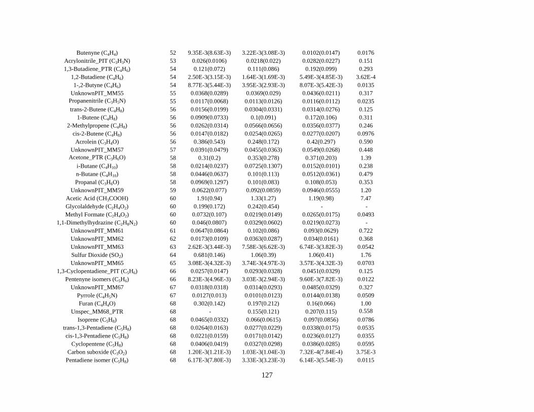
127
Butenyne (C4H4) 52 9.35E-3(8.63E-3) 3.22E-3(3.08E-3) 0.0102(0.0147) 0.0176 Acrylonitrile_PIT (C3H3N) 53 0.026(0.0106) 0.0218(0.022) 0.0282(0.0227) 0.151 1,3-Butadiene_PTR (C4H6) 54 0.121(0.072) 0.111(0.086) 0.192(0.099) 0.293
1,2-Butadiene (C4H6) 54 2.50E-3(3.15E-3) 1.64E-3(1.69E-3) 5.49E-3(4.85E-3) 3.62E-4 1-,2-Butyne (C4H6) 54 8.77E-3(5.44E-3) 3.95E-3(2.93E-3) 8.07E-3(5.42E-3) 0.0135
UnknownPIT_MM55 55 0.0368(0.0289) 0.0369(0.029) 0.0436(0.0211) 0.317 Propanenitrile (C3H5N) 55 0.0117(0.0068) 0.0113(0.0126) 0.0116(0.0112) 0.0235 trans-2-Butene (C4H8) 56 0.0156(0.0199) 0.0304(0.0331) 0.0314(0.0276) 0.125
1-Butene (C4H8) 56 0.0909(0.0733) 0.1(0.091) 0.172(0.106) 0.311 2-Methylpropene (C4H8) 56 0.0262(0.0314) 0.0566(0.0656) 0.0356(0.0377) 0.246
cis-2-Butene (C4H8) 56 0.0147(0.0182) 0.0254(0.0265) 0.0277(0.0207) 0.0976 Acrolein (C3H4O) 56 0.386(0.543) 0.248(0.172) 0.42(0.297) 0.590
UnknownPIT_MM57 57 0.0391(0.0479) 0.0455(0.0363) 0.0549(0.0268) 0.448 Acetone_PTR (C3H6O) 58 0.31(0.2) 0.353(0.278) 0.371(0.203) 1.39
i-Butane (C4H10) 58 0.0214(0.0237) 0.0725(0.1307) 0.0152(0.0101) 0.238 n-Butane (C4H10) 58 0.0446(0.0637) 0.101(0.113) 0.0512(0.0361) 0.479 Propanal (C3H6O) 58 0.0969(0.1297) 0.101(0.083) 0.108(0.053) 0.353
UnknownPIT_MM59 59 0.0622(0.077) 0.092(0.0859) 0.0946(0.0555) 1.20 Acetic Acid (CH3COOH) 60 1.91(0.94) 1.33(1.27) 1.19(0.98) 7.47 Glycolaldehyde (C2H4O2) 60 0.199(0.172) 0.242(0.454) - - Methyl Formate (C2H4O2) 60 0.0732(0.107) 0.0219(0.0149) 0.0265(0.0175) 0.0493
1,1-Dimethylhydrazine (C2H8N2) 60 0.046(0.0807) 0.0329(0.0602) 0.0219(0.0273) - UnknownPIT_MM61 61 0.0647(0.0864) 0.102(0.086) 0.093(0.0629) 0.722 UnknownPIT_MM62 62 0.0173(0.0109) 0.0363(0.0287) 0.034(0.0161) 0.368 UnknownPIT_MM63 63 2.62E-3(3.44E-3) 7.58E-3(6.62E-3) 6.74E-3(3.82E-3) 0.0542 Sulfur Dioxide (SO2) 64 0.681(0.146) 1.06(0.39) 1.06(0.41) 1.76 UnknownPIT_MM65 65 3.08E-3(4.32E-3) 3.74E-3(4.97E-3) 3.57E-3(4.32E-3) 0.0703
1,3-Cyclopentadiene_PIT (C5H6) 66 0.0257(0.0147) 0.0293(0.0328) 0.0451(0.0329) 0.125 Pentenyne isomers (C5H6) 66 8.23E-3(4.96E-3) 3.03E-3(2.94E-3) 9.60E-3(7.82E-3) 0.0122
UnknownPIT_MM67 67 0.0318(0.0318) 0.0314(0.0293) 0.0485(0.0329) 0.327 Pyrrole (C4H5N) 67 0.0127(0.013) 0.0101(0.0123) 0.0144(0.0138) 0.0509 Furan (C4H4O) 68 0.302(0.142) 0.197(0.212) 0.16(0.066) 1.00
Unspec_MM68_PTR 68 - 0.155(0.121) 0.207(0.115) 0.558 Isoprene (C5H8) 68 0.0465(0.0332) 0.066(0.0615) 0.097(0.0856) 0.0786
trans-1,3-Pentadiene (C5H8) 68 0.0264(0.0163) 0.0277(0.0229) 0.0338(0.0175) 0.0535 cis-1,3-Pentadiene (C5H8) 68 0.0221(0.0159) 0.0171(0.0142) 0.0236(0.0127) 0.0355
Cyclopentene (C5H8) 68 0.0406(0.0419) 0.0327(0.0298) 0.0386(0.0285) 0.0595 Carbon suboxide (C3O2) 68 1.20E-3(1.21E-3) 1.03E-3(1.04E-3) 7.32E-4(7.84E-4) 3.75E-3
Pentadiene isomer (C5H8) 68 6.17E-3(7.80E-3) 3.33E-3(3.23E-3) 6.14E-3(5.54E-3) 0.0115

128
UnknownPIT_MM69 69 0.0372(0.0436) 0.0413(0.0336) 0.0529(0.0294) 0.420 Cyclopentane (C5H10) 70 8.20E-4(9.93E-4) 2.39E-3(2.45E-3) 1.58E-3(1.10E-3) 0.0119
1-Pentene (C5H10) 70 0.0177(0.0199) 0.0265(0.0275) 0.0325(0.0285) 0.0832 2-Methyl-1-Butene (C5H10) 70 9.66E-3(1.25E-2) 1.16E-2(1.17E-2) 0.0124(0.0083) 0.0256
trans-2-Pentene (C5H10) 70 0.0132(0.0163) 0.0121(0.0121) 0.0165(0.0109) 0.0333 Methacrolein (C4H6O) 70 0.0426(0.0471) 0.0458(0.0381) 0.0803(0.0666) 0.102
Methylvinylketone (MVK, C4H6O) 70 0.227(0.328) 0.221(0.172) 0.302(0.196) 0.421 Crotonaldehyde (C4H6O) 70 0.182(0.238) 0.209(0.167) 0.193(0.109) 0.494
3-Methyl-1-Butene (C5H10) 70 3.28E-3(3.87E-3) 4.44E-3(5.18E-3) 2.69E-3(2.59E-3) 0.0103 cis-2-Pentene (C5H10) 70 0.0315(0.0274) 0.0446(0.0412) 0.041(0.027) 0.0487
2-Methyl-2-Butene (C5H10) 70 0.0147(0.0081) 0.0306(0.0293) 0.0261(0.0167) 0.0269 2,5-Dihydrofuran (C4H6O) 70 0.0153(0.0259) 3.81E-3(9.82E-3) 1.27E-3(2.54E-3) -
UnknownPIT_MM71 71 0.0311(0.0307) 0.0458(0.0398) 0.0612(0.0329) 0.3853 Acrylic Acid_NI_PT_CIMS (C3H4O2) 72 9.74E-3(3.10E-2) 0.0388(0.0276) 0.0443(0.0403) 0.153
Unspec_MM72 _PTR 72 3.04E-2(2.08E-2) 0.0874(0.0689) 0.101(0.067) 0.191 2,2-Dimethylpropane (C5H12) 72 1.24E-4(1.61E-4) 3.60E-4(7.47E-4) 1.89E-4(2.19E-4) 4.97E-3
i-Pentane (C5H12) 72 8.63E-3(1.31E-2) 2.73E-2(3.58E-2) 7.32E-3(5.40E-3) 0.136 n-Pentane (C5H12) 72 0.0172(0.0239) 0.0368(0.0408) 0.0225(0.018) 0.212 n-Butanal (C4H8O) 72 0.0226(0.0264) 0.0241(0.0216) 0.0313(0.0182) 0.114
Methyl Ethyl Ketone (MEK, C4H8O) 72 0.105(0.143) 0.121(0.112) 0.118(0.062) 0.422 2-Methylpropanal (C4H8O) 72 0.0439(0.0519) 0.043(0.048) 0.0256(0.0199) 0.0924 Tetrahydrofuran (C4H8O) 72 1.59E-3(1.31E-3) 4.98E-4(5.74E-4) 1.74E-3(1.02E-3) 6.37E-3
UnknownPIT_MM73 73 0.0412(0.0551) 0.0575(0.0515) 0.0791(0.0497) 0.645 UnknownPIT_MM74 74 0.228(0.17) 0.345(0.323) 0.547(0.408) 3.33
Ethyl Formate (C3H6O2) 74 0.0126(0.0072) 9.91E-3(1.03E-2) 7.87E-3(5.40E-3) 0.0239 1-Butanol (C4H10O) 74 0.208(0.268) 0.098(0.118) 0.0292(0.016) 1.18
Methyl Acetate (C3H6O2) 74 0.259(0.139) 0.17(0.135) 0.0996(0.058) 0.277 UnknownPIT_MM75 75 0.0177(0.0399) 0.0223(0.0243) 0.0405(0.0223) 0.470
Glycolic Acid_NI_PT_CIMS (C2H4O3) 76 4.55E-3(6.68E-3) 0.038(0.039) 0.0184 0.0904 UnknownPIT_MM76 76 0.0158(0.0098) 0.0327(0.0299) 0.0337(0.016) 0.443 UnknownPIT_MM77 77 0.0312(0.0143) 0.0246(0.0182) 0.022(0.0094) 0.201 Benzene_PTR (C6H6) 78 0.451(0.287) 0.184(0.17) 0.617(0.591) 0.586
Divinylacetylene (C6H6) 78 6.81E-3(5.51E-3) 2.61E-3(2.05E-3) 9.16E-3(6.40E-3) 0.0158 UnknownPIT_MM79 79 0.0409(0.0418) 0.032(0.0329) 0.0457(0.0296) 0.420 UnknownPIT_MM80 80 0.361(0.206) 0.352(0.279) 0.765(0.47) 0.907
Methyl Cyclopentadiene ( isomer 1, C6H8) 80 5.73E-3(5.25E-3) 9.00E-3(1.20E-2) 0.0146(0.0119) 0.0282 Methyl Cyclopentadiene ( isomer 2, C6H8) 80 5.39E-3(5.59E-3) 9.11E-3(1.21E-2) 0.0141(0.0152) 0.0309
Hexenyne (C6H8) 80 6.19E-3(4.45E-3) 3.73E-3(4.74E-3) 0.011(0.0085) 0.0208 UnknownPIT_MM81 81 0.0467(0.0588) 0.0397(0.0341) 0.0641(0.0442) 0.455

129
1-Methylpyrrole (C5H7N) 81 0.0119(0.0194) 3.44E-3(4.51E-3) 3.70E-3(5.12E-3) 0.0147 UnknownPIT_MM82 82 0.203(0.171) 0.243(0.198) 0.356(0.23) 2.91
3-Methylfuran (C5H6O) 82 0.0129(0.0099) 0.0207(0.0173) 0.0291(0.014) 0.0725 cis-1,3-Hexadiene (C6H10) 82 1.89E-3(1.52E-3) 2.01E-3(2.01E-3) 1.67E-3(6.41E-4) 4.46E-3
trans-1,3-Hexadiene (C6H10) 82 3.73E-3(2.27E-3) 4.37E-3(3.83E-3) 5.92E-3(3.57E-3) 7.65E-3 1-Methylcyclopentene (C6H10) 82 0.0117(0.0069) 0.016(0.0154) 0.0185(0.0116) 0.0194
Cyclohexene (C6H10) 82 0.0116(0.0101) 0.0114(0.0095) 0.015(0.0103) 0.0153 Other C6H10 (isomer_1) 82 1.50E-3(1.62E-3) 1.05E-3(1.07E-3) 1.91E-3(2.06E-3) 1.42E-3 Other C6H10 (isomer_2) 82 1.71E-3(1.39E-3) 1.90E-3(1.77E-3) 3.60E-3(2.60E-3) 3.64E-3 Other C6H10 (isomer_3) 82 0.0155(0.0131) 0.0107(0.0103) 0.0204(0.0125) 0.0162 2-Methylfuran (C5H6O) 82 0.159(0.1) 0.213(0.211) 0.199(0.1) 0.537 Other C6H10 (isomer_4) 82 2.94E-3(3.03E-3) 4.35E-3(4.57E-3) 4.38E-3(3.47E-3) 8.01E-3 Other C6H10 (isomer_5) 82 1.31E-3(1.52E-3) 2.04E-3(2.07E-3) 2.44E-3(1.76E-3) 3.85E-3
1-Methylpyrazole (C4H6N2) 82 5.09E-3(4.56E-3) 6.27E-3(5.94E-3) 6.56E-3(4.17E-3) 0.0276 Cyclopentenone (C5H6O) 82 0.0748(0.0994) 0.304(0.414) 0.172(0.13) 0.201
UnknownPIT_MM83 83 0.0552(0.0812) 0.0615(0.0534) 0.078(0.049) 0.934 1-Methylcyclopentane (C6H12) 84 4.54E-3(6.39E-3) 5.66E-3(6.84E-3) 2.64E-3(1.99E-3) 0.0151
Pentenone_PIT (C5H8O) 84 0.231(0.233) 0.335(0.29) 0.474(0.328) 3.78 2-Methyl-1-Pentene (C6H12) 84 0.0674(0.0643) 0.0603(0.0512) 0.084(0.063) 0.117
1-Hexene (C6H12) 84 0.0673(0.0561) 0.0622(0.0547) 0.0842(0.0637) 0.0114 Cyclohexene (C6H12) 84 1.74E-3(2.31E-3) 2.42E-3(2.20E-3) 9.75E-4(6.65E-4) 5.68E-3
Hexenes (sum of 3 isomers, C6H12) 84 0.0571(0.0312) 0.063(0.0696) 0.0935(0.0708) 9.60E-3 cis-2-Hexene (C6H12) 84 0.0147(0.0115) 0.0204(0.0259) 0.0271(0.0154) 5.46E-3
Cyclopentanone (C5H8O) 84 0.0834(0.0425) 0.138(0.147) 0.13(0.079) 0.199 2-Methyl-2-Butenal (C5H8O) 84 5.91E-3(5.11E-3) 8.15E-3(7.91E-3) 6.96E-3(4.24E-3) 0.0230
UnknownPIT_MM85 85 0.0466(0.0867) 0.0481(0.0439) 0.0695(0.0436) 0.768 UnknownPIT_MM86 86 0.249(0.166) 0.367(0.305) 0.513(0.318) 3.27
2,2-Dimethylbutane (C6H14) 86 4.41E-5(7.79E-5) 5.12E-5(1.21E-4) - 2.36E-3 n-Hexane (C6H14) 86 9.23E-3(1.26E-2) 2.11E-2(2.62E-2) 0.0143(0.0115) 0.110
2,3-Butadione (C4H6O2) 86 0.146(0.179) 0.19(0.166) 0.217(0.134) 0.694 3-Methylpentane (C6H14) 86 3.18E-3(5.30E-3) 4.91E-3(6.28E-3) 1.14E-3(7.84E-4) 0.0142
2-Methylbutanal (C5H10O) 86 0.0422(0.0464) 0.0445(0.0547) 0.025(0.0216) 0.0920 3-Methyl-2-Butanone (C5H10O) 86 0.0228(0.0239) 0.0284(0.027) 0.0196(0.0116) 0.0390
2-Pentanone (C5H10O) 86 0.0524(0.0597) 0.0378(0.0337) 0.0314(0.0185) 0.0966 3-Pentanone (C5H10O) 86 0.03(0.0249) 0.0293(0.0278) 0.0238(0.013) 0.0647
Vinyl Acetate (C4H6O2) 86 3.29E-4(9.88E-4) - 1.05E-3(2.10E-3) - Methyl Acrylate (C4H6O2) 86 8.45E-3(4.82E-3) 7.74E-3(5.46E-3) 8.83E-3(5.98E-3) 0.0454
2,3-Dihydro-1,4-Dioxin (C4H6O2) 86 2.53E-3(4.32E-3) 2.32E-3(2.72E-3) 4.16E-3(3.98E-3) 0.0158 UnknownPIT_MM87 87 0.0286(0.0402) 0.0326(0.029) 0.0497(0.0258) 0.449

130
Pyruvic Acid_NI_PT_CIMS (C3H4O3) 88 8.87E-3(1.12E-2) 0.0189(0.0218) 0.0128(0.0141) 0.269 UnknownPIT_MM88 88 0.0593(0.0476) 0.12(0.114) 0.141(0.093) 0.906
Methyl Propanoate (C4H8O2) 88 9.82E-3(1.24E-2) 4.77E-3(4.59E-3) 4.14E-3(2.25E-3) 2.42E-3 UnknownPIT_MM89 89 9.93E-3(1.19E-2) 1.67E-2(1.50E-2) 2.28E-2(1.08E-2) 0.286 UnknownPIT_MM90 90 0.0218(0.0225) 0.0311(0.0261) 0.0486(0.0269) 0.789 UnknownPIT_MM91 91 0.0256(0.0207) 0.0239(0.0184) 0.0256(0.0099) 0.215
Toluene_PTR (C6H5CH3) 92 0.174(0.127) 0.141(0.121) 0.249(0.118) 0.488 Heptadiyne (isomer 1, C7H8) 92 2.03E-3(2.16E-3) 1.63E-3(1.80E-3) 3.91E-3(2.91E-3) 5.23E-3 Heptadiyne (isomer 2, C7H8) 92 2.41E-3(2.28E-3) 3.54E-4(5.33E-4) 4.96E-3(4.49E-3) 1.57E-3
UnknownPIT_MM93 93 0.0477(0.0723) 0.0388(0.0357) 0.0543(0.0381) 0.684 Phenol (C6H5OH) 94 0.453(0.192) 0.335(0.377) - -
UnknownPIT_MM94 94 - - 0.424(0.346) 2.08 Methyl Diazine (isomer 1, C5H6N2) 94 0.0105(0.0056) 0.0139(0.0131) 0.013(0.0067) 0.0435 Methyl Diazine (isomer 2, C5H6N2) 94 9.24E-3(1.20E-2) 6.23E-3(5.34E-3) 5.32E-3(9.95E-4) 8.96E-3 Methyl Diazine (isomer 3, C5H6N2) 94 2.21E-3(3.05E-3) 3.29E-3(5.85E-3) 4.90E-3(3.52E-3) -
UnknownPIT_MM95 95 0.0962(0.1441) 0.0776(0.0746) 0.111(0.08) 0.982 UnknownPIT_MM96 96 0.456(0.507) 0.613(0.593) 0.812(0.619) 8.72 2-Ethylfuran (C6H8O) 96 9.38E-3(7.36E-3) 1.36E-2(1.45E-2) 0.0156(0.0074) 0.0482
1-Methylcyclohexene (C7H12) 96 6.99E-3(4.81E-3) 9.87E-3(9.63E-3) 8.30E-3(5.50E-3) 0.0104 2,5-Dimethylfuran (C6H8O) 96 0.0208(0.0141) 0.0346(0.0364) 0.0358(0.0216) 0.0763
3-Furaldehyde (C5H4O2) 96 0.0118(0.0087) 0.0214(0.0217) 0.0142(0.0093) 0.0588 2-Furaldehyde (C5H4O2) 96 0.279(0.249) 0.521(0.562) 0.266(0.179) 0.647
Cyclopentenedione (C5H4O2) 96 6.84E-3(8.33E-3) 0.012(0.016) 9.50E-3(8.30E-3) 0.0189 UnknownPIT_MM97 97 0.0928(0.1799) 0.0822(0.0787) 0.12(0.09) 1.45 UnknownPIT_MM98 98 0.185(0.23) 0.292(0.26) 0.4(0.301) 3.32
1-Heptene (C7H14) 98 0.0524(0.049) 0.047(0.0434) 0.0566(0.0399) 0.0881 1-Methylcyclohexane (C7H14) 98 2.81E-3(3.45E-3) 4.42E-3(4.42E-3) 2.26E-3(1.56E-3) 8.57E-3
UnknownPIT_MM99 99 0.0338(0.055) 0.0471(0.0424) 0.0676(0.0493) 0.591 UnknownPIT_MM100 100 0.143(0.128) 0.285(0.267) 0.386(0.265) 2.12
n-Hexanal (C6H12O) 100 0.0163(0.0173) 0.0257(0.0278) 0.0166(0.0122) 0.159 n-Heptane (C7H16) 100 0.0211(0.0241) 0.027(0.0279) 0.0168(0.0138) 0.0481
Methyl Methacrylate (C5H8O2) 100 0.0326(0.0271) 0.0374(0.0329) 0.0272(0.0153) 0.0759 3-Hexanone (C6H12O) 100 0.033(0.0289) 0.0308(0.0267) 0.0352(0.0231) 0.0536 2-Hexanone (C6H12O) 100 0.0153(0.0172) 0.0134(0.0127) 0.0106(0.0077) 9.67E-3 UnknownPIT_MM101 101 0.0265(0.0344) 0.0398(0.0362) 0.0532(0.0352) 0.548 UnknownPIT_MM102 102 0.104(0.101) 0.174(0.163) 0.227(0.172) 1.73
Methyl Butanoate (C5H10O2) 102 2.68E-3(1.93E-3) 0.0157(0.0358) 2.94E-3(1.59E-3) 4.20E-3 Ethynyl Benzene (C8H6) 102 0.0526(0.0776) 6.55E-3(5.70E-3) 0.0163(0.0198) 0.0425 UnknownPIT_MM103 103 0.0807(0.0657) 0.0692(0.0421) 0.0865(0.0598) 0.989

131
Benzenenitrile (C7H5N) 103 0.0557(0.0392) 0.0596(0.0609) 0.0308(0.0221) 0.101 UnknownPIT_MM104 104 0.0711(0.0516) 0.0697(0.0581) 0.11(0.07) 0.720
Styrene (C8H8) 104 0.0881(0.1051) 0.0491(0.0386) 0.0783(0.0747) 0.117 UnknownPIT_MM105 105 0.03(0.0278) 0.0238(0.0217) 0.0402(0.0173) 0.262 Ethylbenzene (C8H10) 106 0.0401(0.0507) 0.0385(0.04) 0.0396(0.0294) 0.104 m,p-Xylene (C8H10) 106 0.0692(0.0742) 0.0978(0.1049) 0.111(0.08) 0.178
o-Xylene (C8H10) 106 0.0308(0.0369) 0.0343(0.0372) 0.0308(0.0176) 0.101 Benzaldehyde (C7H6O) 106 0.243(0.398) 0.194(0.181) 0.155(0.093) 0.583 UnknownPIT_MM107 107 0.0428(0.0558) 0.0342(0.0285) 0.0539(0.0383) 0.626 UnknownPIT_MM108 108 0.226(0.297) 0.162(0.138) 0.348(0.279) 2.60
2-Ethylpyrazine (C6H8N2) 108 4.14E-3(3.23E-3) 6.95E-3(7.03E-3) 6.72E-3(3.82E-3) 0.0212 UnknownPIT_MM109 109 0.0569(0.1257) 0.0427(0.0383) 0.0765(0.0595) 0.724
Resorcinol_NI_PT_CIMS (C6H6O2) 110 0.189(0.197) 1.37(1.24) 1.15(1.04) 2.69 UnknownPIT_MM110 110 0.172(0.29) 0.242(0.218) 0.472(0.41) 4.86
Octadiene (C8H14) 110 0.0231(0.0154) 0.0284(0.0252) 0.0308(0.0173) 0.0503 UnknownPIT_MM111 111 0.0392(0.0685) 0.0414(0.0413) 0.0898(0.0755) 0.867 UnknownPIT_MM112 112 0.138(0.179) 0.268(0.259) 0.397(0.32) 3.06
1-Octene (C8H16) 112 0.0522(0.0531) 0.0476(0.0476) 0.0388(0.0273) 0.0867 UnknownPIT_MM113 113 0.0348(0.0488) 0.0477(0.0468) 0.0744(0.0588) 0.677 UnknownPIT_MM114 114 0.116(0.159) 0.215(0.21) 0.299(0.231) 2.35
n-Octane (C8H18) 114 0.019(0.0205) 0.024(0.0237) 0.0125(0.0088) 0.0390 UnknownPIT_MM115 115 0.0307(0.0386) 0.0465(0.04) 0.0663(0.0508) 0.548 UnknownPIT_MM116 116 0.139(0.205) 0.175(0.158) 0.34(0.255) 2.13
Indene (C9H8) 116 0.0305(0.0292) 0.0204(0.0198) 0.0333(0.0369) 0.0506 UnknownPIT_MM117 117 0.0407(0.0547) 0.0355(0.0299) 0.0592(0.0379) 0.486
Benzofuran_PIT (C8H6O) 118 0.103(0.102) 0.0874(0.0736) 0.167(0.113) 0.908 Indane (C9H10) 118 8.70E-3(6.85E-3) 7.11E-3(6.13E-3) 6.39E-3(3.70E-3) 0.0102
1-Propenylbenzene (C9H10) 118 4.60E-3(4.95E-3) 2.38E-3(2.66E-3) 3.82E-3(2.66E-3) 1.16E-3 alpha-Methylstyrene (C9H10) 118 4.69E-3(2.89E-3) 3.39E-3(3.34E-3) 6.23E-3(4.82E-3) 3.89E-3
3-Methylstyrene (C9H10) 118 0.02(0.0128) 0.0169(0.0171) 0.022(0.016) 0.0342 2-Methylstyrene (C9H10) 118 0.0135(0.0093) 0.01(0.0101) 0.011(0.0071) 0.0194
2-Propenylbenzene (C9H10) 118 5.95E-3(4.77E-3) 5.99E-3(5.80E-3) 6.03E-3(3.61E-3) 8.69E-3 4-Methylstyrene (C9H10) 118 6.21E-3(4.64E-3) 8.49E-3(9.25E-3) 7.66E-3(3.90E-3) 0.0134 UnknownPIT_MM119 119 0.0315(0.036) 0.0238(0.0223) 0.0587(0.0386) 0.577
1-Ethyl-3-,4-Methylbenzene (C9H12) 120 0.0163(0.0183) 0.0228(0.0238) 0.0323(0.0264) 0.0433 1,2,4-Trimethylbenzene (C9H12) 120 0.0166(0.0209) 0.0242(0.0254) 0.0212(0.0134) 0.0555
1-Ethyl-2-Methylbenzene (C9H12) 120 0.0111(0.0094) 9.71E-3(1.04E-2) 9.50E-3(6.20E-3) 0.0122 1,2,3-Trimethylbenzene (C9H12) 120 0.0183(0.0138) 0.0314(0.0366) 0.0231(0.0196) 0.0291
Isopropylbenzene (C9H12) 120 6.08E-3(4.42E-3) 6.03E-3(6.05E-3) 8.08E-3(7.33E-3) 6.43E-3

132
n-Propylbenzene (C9H12) 120 9.60E-3(6.30E-3) 1.05E-2(9.64E-3) 8.60E-3(6.20E-3) 0.0124 1,3,5-Trimethylbenzene (C9H12) 120 0.0143(0.016) 0.0139(0.0147) 0.0104(0.0064) 0.0212
UnknownPIT_MM121 121 0.0343(0.0504) 0.0317(0.0273) 0.0676(0.0501) 0.525 UnknownPIT_MM122 122 0.114(0.145) 0.129(0.11) 0.332(0.272) 2.02 UnknownPIT_MM123 123 0.0442(0.0643) 0.0487(0.0479) 0.0954(0.0624) 1.13 UnknownPIT_MM124 124 0.139(0.227) 0.216(0.203) 0.465(0.406) 5.10
Nonadiene (C9H16) 124 2.06E-3(2.25E-3) 3.37E-3(3.45E-3) 4.80E-3(3.10E-3) - UnknownPIT_MM125 125 0.0425(0.076) 0.0401(0.0391) 0.118(0.089) 2.93 UnknownPIT_MM126 126 0.116(0.195) 0.151(0.143) 0.28(0.223) 2.74
1-Nonene (C9H18) 126 0.0103(0.0083) 0.012(0.0135) 0.0117(0.0082) 0.0230 UnknownPIT_MM127 127 0.04(0.041) 0.0368(0.0336) 0.0806(0.0602) 0.725
Naphthalene_PTR (C10H8) 128 0.173(0.097) 0.199(0.182) 0.286(0.19) 0.815 Nonane (C9H20) 128 0.013(0.0164) 0.0143(0.0159) 9.20E-3(7.70E-3) 0.0225
UnknownPIT_MM129 129 0.0564(0.0478) 0.0528(0.0481) 0.0998(0.0712) 0.834 UnknownPIT_MM130 130 0.0844(0.1141) 0.116(0.111) 0.225(0.175) 1.87
1-,3-Methyl Indene (C10H10) 130 1.43E-3(1.13E-3) 1.90E-4(4.92E-4) 2.49E-3(2.25E-3) 1.75E-3 1,2-Dihydronaphthalene (C10H10) 130 6.83E-3(4.60E-3) 6.87E-3(8.79E-3) 7.83E-3(4.84E-3) 6.44E-3 1,3-Dihydronaphthalene (C10H10) 130 7.39E-3(4.65E-3) 7.88E-3(9.53E-3) 0.01(0.0057) 7.24E-3
UnknownPIT_MM131 131 0.0374(0.0555) 0.0305(0.0276) 0.0587(0.0419) 0.387 UnknownPIT_MM132 132 0.126(0.168) 0.0988(0.085) 0.24(0.19) 1.33
1-Butenylbenzene (C10H14) 132 2.49E-3(2.57E-3) 2.69E-3(4.86E-3) 4.22E-3(2.15E-3) 1.92E-3 Methylbenzofuran (isomer 4, C9H8O) 132 8.72E-4(2.62E-3) - 2.66E-3(3.95E-3) -
Ethylstyrene (C10H12) 132 4.34E-3(3.49E-3) 3.95E-3(5.65E-3) 5.66E-3(3.55E-3) 2.10E-3 1-Methyl-1-Propenylbenzene (C10H12) 132 0.0321(0.0551) 0.0142(0.0172) 0.0131(0.0106) 5.23E-3 Methylbenzofuran (isomer 1, C9H8O) 132 0.0121(0.0076) 0.0135(0.0156) 0.0114(0.0041) 0.0235 Methylbenzofuran (isomer 2, C9H8O) 132 0.019(0.0118) 0.0229(0.0284) 0.0187(0.0064) 0.0380 Methylbenzofuran (isomer 3, C9H8O) 132 0.0324(0.026) 0.0323(0.0418) 0.0222(0.0073) 0.0517
UnknownPIT_MM133 133 0.0675(0.1622) 0.033(0.0303) 0.0659(0.0508) 0.357 p-Cymene (C10H14) 134 0.117(0.323) 0.056(0.075) 0.0509(0.0519) 0.059
C10H14 non-aromatic (e.g., hexahydronaphthalene) 134 2.39E-3(2.19E-3) 3.54E-3(5.04E-3) 4.84E-3(3.26E-3) - Isobutylbenzene (C10H14) 134 5.06E-3(5.18E-3) 7.89E-3(9.35E-3) 7.31E-3(5.61E-3) 7.55E-3
Methyl-n-Propylbenzene (isomer 1, C10H14) 134 4.38E-3(3.50E-3) 8.70E-3(1.02E-2) 6.99E-3(4.40E-3) 2.45E-3 Methyl-n-Propylbenzene (isomer 2, C10H14) 134 3.69E-3(2.96E-3) 7.41E-3(8.61E-3) 5.39E-3(3.45E-3) 1.73E-3
n-Butylbenzene (C10H14) 134 6.61E-3(6.03E-3) 1.19E-2(1.34E-2) 9.90E-3(6.52E-3) 0.0131 1,4-Diethylbenzene (C10H14) 134 1.54E-3(2.03E-3) 2.72E-3(4.86E-3) 5.68E-3(3.50E-3) 1.76E-3
Ethyl Xylene (isomer 1, C10H14) 134 6.29E-3(6.11E-3) 8.76E-3(1.18E-2) 7.31E-3(4.06E-3) 2.68E-3 Ethyl Xylene (isomer 2, C10H14) 134 4.12E-3(4.10E-3) 4.77E-3(5.98E-3) 4.54E-3(2.71E-3) 1.88E-3
UnknownPIT_MM135 135 0.0432(0.0663) 0.0395(0.0378) 0.18(0.161) 0.526 Monoterpenes_PTR (C10H16) 136 0.146(0.083) 0.253(0.238) 0.619(0.46) 0.695

133
beta-Pinene (C10H16) 136 0.0133(0.0258) 0.0182(0.0238) 0.053(0.0574) 0.0915 D-Limonene (C10H16) 136 0.0249(0.0227) 0.0665(0.0884) 0.277(0.425) 0.0848
Myrcene (C10H16) 136 0.0102(0.0095) 5.51E-3(5.99E-3) 0.0437(0.0665) 0.0355 3-Carene (C10H16) 136 0.0189(0.0403) 0.0179(0.0242) 0.0513(0.0765) 0.0226
gamma-Terpinene (C10H16) 136 5.33E-3(2.52E-3) 4.81E-3(7.48E-3) 0.0109(0.0123) 3.93E-3 Terpinolene (C10H16) 136 6.80E-3(3.17E-3) 7.51E-3(1.06E-2) 0.0114(0.0158) 6.69E-3 alpha-Pinene (C10H16) 136 0.0163(0.0295) 0.0518(0.0884) 0.272(0.429) 0.0837 Camphene (C10H16) 136 9.46E-3(1.53E-2) 2.66E-2(5.49E-2) 0.039(0.0529) 0.0812
iso-Limonene (C10H16) 136 2.87E-4(8.60E-4) 5.76E-3(6.72E-3) 7.37E-3(7.69E-3) 1.80E-3 UnknownPIT_MM137 137 0.0316(0.0481) 0.0462(0.046) 0.172(0.15) 0.737 UnknownPIT_MM138 138 0.0789(0.1041) 0.16(0.156) 0.325(0.265) 3.55 UnknownPIT_MM139 139 0.0257(0.0357) 0.0277(0.0284) 0.0611(0.0499) 0.676 UnknownPIT_MM140 140 0.0572(0.0842) 0.0749(0.0678) 0.148(0.117) 1.22
1-Decene (C10H20) 140 0.0125(0.011) 0.0174(0.02) 0.0227(0.0142) 0.0218 UnknownPIT_MM141 141 0.0252(0.0298) 0.0305(0.0279) 0.0453(0.0301) 0.556 UnknownPIT_MM142 142 0.108(0.163) 0.115(0.098) 0.254(0.196) 2.25
n-Decane (C10H22) 142 0.0148(0.0207) 0.0131(0.0154) 8.68E-3(6.85E-3) 0.0265 UnknownPIT_MM143 143 0.0308(0.0553) 0.0374(0.0328) 0.0629(0.0509) 0.681 UnknownPIT_MM144 144 0.102(0.25) 0.195(0.209) 0.271(0.231) 3.88 UnknownPIT_MM145 145 0.0276(0.0513) 0.0294(0.0264) 0.0583(0.0446) 0.550 UnknownPIT_MM146 146 0.0764(0.1249) 0.0773(0.0673) 0.192(0.149) 1.26 UnknownPIT_MM147 147 0.024(0.0463) 0.0191(0.018) 0.0528(0.04) 0.378
C11 Aromatics_PTR 148 0.0547(0.0331) 0.0844(0.0722) 0.105(0.07) 0.228 UnknownPIT_MM149 149 0.0227(0.0436) 0.0232(0.022) 0.0558(0.0389) 0.376 UnknownPIT_MM150 150 0.0565(0.0795) 0.0894(0.0873) 0.216(0.174) 1.59 UnknownPIT_MM151 151 0.0215(0.0322) 0.0237(0.0221) 0.0575(0.0406) 0.418 UnknownPIT_MM152 152 0.0792(0.079) 0.0976(0.0929) 0.274(0.207) 2.29 UnknownPIT_MM153 153 0.0356(0.0374) 0.0282(0.021) 0.0779(0.0511) 0.574 UnknownPIT_MM154 154 0.0675(0.0923) 0.0614(0.0496) 0.148(0.1) 1.13 1-Undecene (C11H22) 154 0.0136(0.0125) 0.0222(0.0301) 0.0203(0.0096) 0.0364
UnknownPIT_MM155 155 0.0206(0.0335) 0.0151(0.015) 0.0447(0.0285) 0.340 UnknownPIT_MM156 156 0.0638(0.1101) 0.0589(0.0478) 0.146(0.11) 1.20 n-Undecane (C11H24) 156 0.0189(0.02) 0.0287(0.0353) 0.014(0.0078) 0.0429
UnknownPIT_MM157 157 0.0183(0.0356) 0.0149(0.0154) 0.0333(0.0215) 0.257 UnknownPIT_MM158 158 0.0363(0.0641) 0.0428(0.0397) 0.09(0.063) 0.623 UnknownPIT_MM159 159 0.0139(0.0301) 0.0128(0.0156) 0.0242(0.0149) 0.225 UnknownPIT_MM160 160 0.0372(0.0788) 0.0392(0.0387) 0.0994(0.0766) 0.846 UnknownPIT_MM161 161 0.0131(0.0341) 9.18E-3(1.27E-2) 0.0365(0.0267) 0.326 UnknownPIT_MM162 162 0.0375(0.0819) 0.0466(0.0399) 0.112(0.088) 1.11

134
UnknownPIT_MM163 163 8.51E-3(2.69E-2) 0.0104(0.0115) 0.0312(0.0208) 0.253 UnknownPIT_MM164 164 0.0284(0.0485) 0.0423(0.0391) 0.114(0.08) 0.942 UnknownPIT_MM165 165 0.0112(0.0202) 9.60E-3(1.16E-2) 0.0299(0.019) 0.240 UnknownPIT_MM166 166 0.0271(0.0413) 0.0301(0.0301) 0.0917(0.0627) 0.700 UnknownPIT_MM167 167 0.016(0.0274) 0.0126(0.0096) 0.0354(0.0242) 0.362 UnknownPIT_MM168 168 0.0504(0.081) 0.0347(0.0286) 0.125(0.071) 0.747 UnknownPIT_MM169 169 0.0165(0.0313) 8.29E-3(9.87E-3) 0.0344(0.0198) 0.314 UnknownPIT_MM170 170 0.0333(0.0791) 0.0306(0.0268) 0.0819(0.0582) 0.624 UnknownPIT_MM171 171 0.015(0.0326) 7.82E-3(8.37E-3) 0.0204(0.0139) 0.155 UnknownPIT_MM172 172 0.0252(0.0495) 0.0358(0.0338) 0.0524(0.0428) 0.396 UnknownPIT_MM173 173 9.54E-3(2.28E-2) 5.22E-3(7.33E-3) 0.0124(0.0112) 0.157 UnknownPIT_MM174 174 0.0304(0.0711) 0.0296(0.0293) 0.0557(0.0465) 0.527 UnknownPIT_MM175 175 9.19E-3(3.06E-2) 7.90E-3(9.28E-3) 0.0157(0.0109) 0.176 UnknownPIT_MM176 176 0.0189(0.0526) 0.0194(0.0195) 0.0551(0.0437) 0.501 UnknownPIT_MM177 177 7.09E-3(2.04E-2) 4.78E-3(7.85E-3) 0.0209(0.0122) 0.131 UnknownPIT_MM178 178 0.019(0.0466) 0.016(0.015) 0.0681(0.0444) 0.376 UnknownPIT_MM179 179 8.55E-3(3.60E-2) 4.52E-3(5.58E-3) 0.0315(0.0196) 0.104 UnknownPIT_MM180 180 0.0137(0.0379) 0.0111(0.0137) 0.0435(0.0236) 0.383 UnknownPIT_MM181 181 8.55E-3(2.37E-2) 6.13E-3(1.10E-2) 0.0227(0.011) 0.260 UnknownPIT_MM182 182 0.0243(0.0475) 0.0167(0.0178) 0.0648(0.0411) 0.531 UnknownPIT_MM183 183 8.70E-3(2.53E-2) 5.05E-3(4.86E-3) 0.015(0.0092) 0.114 UnknownPIT_MM184 184 0.0142(0.041) 0.0156(0.018) 0.0448(0.0303) 0.327 UnknownPIT_MM185 185 5.65E-3(2.07E-2) 3.67E-3(6.91E-3) 0.0099(0.0115) 0.120 UnknownPIT_MM186 186 0.0116(0.0383) 0.0119(0.0135) 0.0318(0.0233) 0.345 UnknownPIT_MM187 187 4.86E-3(1.92E-2) 2.46E-4(5.54E-3) 0.0119(0.0103) 0.120 UnknownPIT_MM188 188 0.0149(0.05) 0.0153(0.0142) 0.0302(0.0323) 0.356 UnknownPIT_MM189 189 4.85E-3(3.19E-2) 6.18E-3(8.40E-3) 7.71E-3(1.13E-2) 0.203 UnknownPIT_MM190 190 0.0131(0.053) 0.0154(0.0164) 0.0365(0.0337) 0.334 UnknownPIT_MM191 191 8.84E-3(3.35E-2) 4.56E-3(9.08E-3) 0.0132(0.0104) 0.120 UnknownPIT_MM192 192 9.50E-3(2.86E-2) 4.60E-3(8.33E-3) 0.0238(0.0156) 0.295 UnknownPIT_MM193 193 2.26E-3(1.99E-2) 7.74E-4(1.02E-2) 8.10E-3(8.90E-3) 0.135 UnknownPIT_MM194 194 6.19E-3(2.61E-2) 6.79E-3(1.21E-2) 0.0191(0.0119) 0.209 UnknownPIT_MM195 195 6.74E-3(1.88E-2) 4.81E-3(9.40E-3) 0.0138(0.009) 0.146 UnknownPIT_MM196 196 0.0121(0.0333) 9.34E-3(1.21E-2) 0.0334(0.0262) 0.324 UnknownPIT_MM197 197 4.49E-3(2.13E-2) 3.04E-3(6.63E-3) 9.20E-3(1.06E-2) 0.183 UnknownPIT_MM198 198 3.86E-3(2.05E-2) 7.38E-3(9.91E-3) 0.0234(0.0214) 0.262 UnknownPIT_MM199 199 2.08E-3(1.79E-2) - 0.0103(0.0051) 0.131 UnknownPIT_MM200 200 3.29E-3(1.84E-2) 7.78E-3(1.21E-2) 0.0216(0.0161) 0.160 UnknownPIT_MM201 201 4.80E-3(1.99E-2) 2.22E-3(8.58E-3) 4.60E-3(9.30E-3) 0.122

135
UnknownPIT_MM202 202 7.55E-3(3.19E-2) 0.014(0.0189) 0.0186(0.0122) 0.258 UnknownPIT_MM203 203 3.85E-3(3.19E-2) 4.53E-3(1.46E-2) 0.0128(0.0076) 0.138
Sesquiterpenes_PIT (C15H24) 204 0.0167(0.014) 0.0502(0.0758) 0.0448(0.0251) 0.0949 UnknownPIT_MM205 205 9.44E-3(3.70E-2) 0.0232(0.0386) 0.0197(0.0189) 0.344 UnknownPIT_MM206 206 5.45E-3(1.81E-2) 8.24E-3(1.26E-2) 0.0118(0.0132) 0.224 UnknownPIT_MM207 207 7.02E-3(1.68E-2) 1.52E-3(8.22E-3) 0.0154(0.0102) 0.121 UnknownPIT_MM208 208 8.02E-3(1.46E-2) 4.07E-3(1.05E-2) 0.0132(0.0163) 0.128 UnknownPIT_MM209 209 5.26E-3(1.94E-2) 1.89E-3(1.01E-2) 0.0117(0.0107) 0.0775 UnknownPIT_MM210 210 8.78E-3(1.99E-2) 3.88E-3(9.93E-3) 0.0174(0.0139) 0.210 UnknownPIT_MM211 211 8.55E-3(3.06E-2) 2.00E-3(1.12E-2) 0.0149(0.0143) 0.234 UnknownPIT_MM212 212 2.05E-3(1.05E-2) - 7.38E-3(1.08E-2) 0.0942 UnknownPIT_MM213 213 3.12E-4(3.52E-3) 7.75E-4(3.16E-3) 1.34E-3(3.82E-4) 3.45E-3
PM2.5
7.06(1.5) 13.6(7.5) 7.44(5.83) 20.6 Table 8.2 Best estimate emission factors (g kg-1) for four types of fire: prescribed fires in semiarid shrubland and pine-forest understory, and burning
coniferous canopy or organic soils. (See text for discussion.)

136
8.4.4 Some Fundamental Characteristics of Fresh Smoke Revealed by Full Mass Scans
Important impacts of NMOC on smoke plume chemistry include the potential to contribute to O3 and secondary aerosol formation. In broad terms, oxidation of NMOCs in the presence of NOx generates both O3 and secondary organic aerosol (SOA). In general, oxidation of the lower MM NMOCs (volatile organic compounds (VOCs)) tends to generate CO and CO2 as end products and HOx as an intermediate that converts NO to NO2, which photolyzes to produce O3. However, the larger VOCs can also be oxidized to more soluble or less volatile compounds (semivolatile organic compounds or intermediate volatility organic compounds, SVOC and IVOC, respectively). Subsequent oxidation or cooling of IVOC and SVOC can generate O3 and SOA on various time-scales [Finlayson-Pitts and Pitts, 2000]. The SVOC and IVOC already present in fresh emissions are perhaps more likely to contribute to SOA on shorter time scales: e.g. during the several hours that many biomass burning plumes exist as coherent isolated entities in the boundary layer (or in smog chamber experiments) [Yokelson et al., 2009; Hennigan et al., 2011]. Thus, estimating or modeling the potential for smoke photochemistry to generate O3 or secondary particle mass requires realistic estimates of the relative amounts of total VOC, IVOC, SVOC, NOx, etc., in fresh smoke and the chemical behavior of the species in these categories. In Table 8.3 we address the question of relative amounts by computing estimates of the lumped categories mentioned above that take unidentified species into account. We also show ratios between these lumped categories and/or NOx and PM2.5 for each of the four fuel types in our broad classification scheme.
Semiarid
Shrublands Pine
Understory
Average Pine & Shrub
Coniferous Canopy
Organic Soil Quantity or Ratio
PM2.5 7.06 13.55 10.31 7.44 20.60
NOx "as NO" 2.18 2.55 2.37 2.40 0.67
ΣNMOC 25.24 27.64 26.44 34.45 178.89
Σ(IVOC+SVOC) 8.71 11.26 9.99 17.10 114.78
ΣUnidentified NMOC 7.81 8.62 8.21 16.20 129.29
ΣNMOC/PM2.5 3.58 2.04 2.81 4.63 8.68
Σ(IVOC+SVOC)/PM2.5 1.23 0.83 1.03 2.30 5.57
Σ(IVOC+SVOC)/ΣNMOC 0.35 0.41 0.38 0.50 0.64
ΣNMOC/"NOx as NO" 11.58 10.84 11.21 14.35 267.00
Percent NMOC Unidentified 31 31 31 47 72
Table 8.3 Calculation of some lumped category emission factors in g kg-1 and indicated mass ratios or
percentages (see text for category definitions).
Table 8.3 shows an average NMOC/PM2.5 ratio for our two main fuel types of about three with higher values up to about nine possible for organic soil. The gas-phase NMOC to condensed-phase organic aerosol (OA) ratio would be higher since biomass burning PM2.5 is typically about 60-80% OA (Reid et al., 2005). It is also of interest to estimate the IVOC and SVOC fraction of the gas-phase NMOC to roughly assess the potential amount of SOA production on the time scale of a few hours. Definitions of SVOC and IVOC are not straightforward or identical for all users of these terms. For instance, the EU and USEPA broadly classify SVOC as compounds with boiling points above 250º and 200º C, respectively, but the USEPA includes phenol as an SVOC despite it having a boiling point of 182º C. In a review

137
article on SVOC, Weschler and Nazaroff [2008] adopt a working definition of SVOC as having vapor pressure lower than 10 Pa at room temperature. We note that toluene is well established as an OA precursor and so we have based a crude estimate of the total intermediate and semivolatile gas-phase organic compounds (IVOC+SVOC) as the sum of species at or above the mass of toluene. With this arbitrary choice, for both main fuel types (i.e. pine understory and semiarid shrubland), we estimate that ~38% of the mass of total NMOC fall in the intermediate to semi volatile range and that IVOC+SVOC are roughly equal in abundance to initial PM2.5. If we assume OA is 70% of PM2.5 and a SOA yield of 40% for the IVOC and SVOC, then OA could increase by ~60% on short time scales just from the co-emitted IVOC and SVOC alone. This is not unreasonable and a little below the highest level of SOA formation observed to date in real biomass burning plumes (e.g. factor of two in Yokelson et al., 2009). It’s not likely that maximum SOA would occur in all plumes (e.g. a small initial decrease in OA was observed by Akagi et al. (2012a)) dependent on factors such as dilution rate, temperature, humidity, oxidant levels, etc. Investigating the complex factors governing plume evolution is the province of plume evolution measurements and models. Here we simply provide a realistic estimate of the amount of precursors that includes rarely measured species or those that are presently unidentified. We also note that higher precursor/OA ratios are suggested by Table 8.3 for the coniferous canopy and organic soil fuels which are thought to be relatively more important in wildfires.
Secondary inorganic aerosol (SIA) could be formed primarily from nitrogen containing gases (NH3 to ammonium and NOx to nitrate) and SO2 (to sulfate). The emissions of these precursor gases are heavily dependent on fuel chemistry with foliage and crop residue having elevated levels. In this study the emission factors of the NH3, NOx, and SO2 sum to about 4 g kg-1 compared to a generic EFPM2.5 of ~10 g kg-1, suggesting that SIA should not be neglected in smoke plume models. Substantial SIA has been measured in the field in biomass burning plumes [Yokelson et al., 2009; Alvarado et al., 2010; Akagi et al., 2012a].
The initial NMOC/NOx mass ratio is ~11 for the two main fuel types investigated in both the lab and field with much higher values (~267) observed in the lab for smoldering organic soil. Since NOx is rapidly converted to PAN and particle nitrate downwind [Yokelson et al., 2009; Alvarado et al., 2010; Akagi et al., 2012a] it is likely that O3 formation would be NOx-limited over most of the lifetime of smoke plumes in the absence of mixing with additional NOx sources (see next chapter). Low NOx levels also favor SOA formation when biomass burning smoke is photochemically aged in chamber experiments [e.g. Grieshop et al., 2009].
The prospects for fully mechanistic modeling of smoke plumes and the adequacy of using only known, measured species can be assessed from Table 8.3 as well. For the two main fuel types ~31% of the NMOC mass is unidentified and ~72% of the mass of NMOC is unidentified for the one lab fire in smoldering Alaskan organic soil. In addition, the majority of unidentified NMOC are in our “IVOC+SVOC” category suggesting the need to model SOA with semi-empirical approaches for some time to come [Robinson et al., 2007].
Two important examples of how this data set could improve modeling of global biomass burning are described next. (1) Peat combustion is a major global type of biomass combustion especially in El-Niño years (Page et al., 2002; Akagi et al., 2011). In that light, we note that our laboratory smoldering organic soil fire had the largest PM2.5 emissions (20.6 g kg-1), the largest EFNMOC (179 g kg-1), the largest ratio of NMOC to PM2.5 (~8.7), and the largest fraction of NMOC in our “IVOC+SVOC” category (0.64). This fuel type may have very high potential for SOA, but it is also the least well characterized. Table 8.2 and

138
Table 8.3 provide important new emissions data for smoldering organic soils, but also highlight the need for further study of this source. (2) Akagi et al. [2011] estimated global NMOC emissions from biomass burning using only previously available information. Their estimate of total EFNMOC (including unmeasured species) for temperate forests of 23.7 g kg-1 (their Table S4) is close to the total EFNMOC measured in this work for the pine-forest understory fires (~27.6 g kg-1). Akagi et al. [2011] derived an estimate of total EFNMOC of 97.3 g kg-1 for peatland fires, which is actually well below the value of 179 g kg-1 measured for smoldering organic soils in this work. The global NMOC estimate of Akagi et al. [2011] was 4-7 times larger than some previous estimates of organic trace gas emissions from fires that ignored oxygenated organic compounds and unidentified species, but it is strongly supported by this work suggesting that global model runs with much larger NMOC emissions per unit mass of biomass burned are needed.
8.4.5 Gas-phase Hazardous Air Pollutants Present in Initial Prescribed Fire Smoke
The health effects of smoke constituents are an important aspect of understanding the impact of prescribed burning. A number of compounds that were measured in this study appear on the USEPA list of hazardous air pollutants (HAPS) [U.S. EPA, 2005] and many are also on the USFDA list of harmful and potentially harmful constituents of tobacco smoke (HPHC) [U.S. FDA, 2012]. The list of compounds identified in this study common to each list is given in Table 8.4. Isocyanic acid (HNCO) is not on either list, but has been connected to smoke-related health effects through detailed biochemical studies [Wang et al., 2007]. A previous publication noted this connection and pointed out the need for additional research on this compound [Roberts et al, 2011]. The exposure to toxic compounds in the initial smoke produced by prescribed fires was estimated using the EFs Table 8.2 of this chapter. Alternatively, Sharkey et al. [1997] coupled a few literature measurements of emission ratios to CO for air toxics in smoke with measurements of wildland firefighter exposure to CO to estimate firefighter exposure to those air toxics and then compared that with permissible exposure limits as set by NIOSH or OSHA. Following that approach a more comprehensive assessment of firefighter exposure is now available based on the data we present in Table 8.2 coupled with measurements of CO on the perimeter of South Carolina prescribed fires [Akagi et al., 2012c]. We note however, that comparisons to exposure limits for individual species ignore possible synergistic effects of multiple pollutants acting in concert [Menser and Heggestad, 1966]. Further, additional air toxics could be present among the unidentified species and the mix of air toxics evolves rapidly as smoke ages since e.g. 1,3-butadiene has a lifetime of several hours while substantial PAN and O3 can form in smoke plumes on similar time scales [Akagi et al., 2012a; Gregg et al., 2003]. A reasonable assessment of smoke health effects would also necessarily include consideration of the health effects of the particles [Pope and Dockery, 2006]. Since smoke could affect health via numerous, poorly understood, coupled mechanisms, empirical studies that relate exposure to health outcomes are also valuable for assessing risk [Rappold et al., 2011]. In summary, a complete assessment of smoke health effects is clearly beyond the scope of this paper, but the data in Table 8.4 contribute to such an effort.

139
Compound Molecular Wt. EPA HAP FDA HPHC Ammonia 17 No Yes Hydrogen Cyanide 27 Yes Yes Formaldehyde 30 Yes Yes Methanol 32 Yes No Hydrochloric Acid 36.5 Yes No Acetonitrile 41 Yes No Acetaldehyde 44 Yes Yes Acrylonitrile 53 Yes Yes 1,3-Butadiene 54 Yes Yes Acrolein 56 Yes Yes Propionaldehyde 58 Yes Yes Acetone 58 No Yes 1,1-Dimethylhydrazine 60 Yes No Furan 68 No Yes Crotonaldehyde 70 No Yes Acrylic Acid 72 Yes No Methyl Ethyl Ketone 72 No Yes Benzene 78 Yes Yes Vinyl Acetate 86 Yes Yes Hexane 86 Yes No Toluene 92 Yes Yes Phenol 94 Yes Yes Methyl Methacrylate 100 Yes No Styrene 104 Yes Yes Xylenes 106 Yes No Ethylbenzene 106 Yes Yes Catechol 110 Yes Yes Naphthalene 128 Yes Yes
Table 8.4 The list of compounds identified in this study that are also considered either hazardous air pollutants (EPA) or harmful and potentially harmful constituents in tobacco smoke (FDA).
8.4.6 Particle Elemental Carbon Emission Factors and Metal Profiles
Extrapolation of laboratory PM measurements to field fires in the natural environment should consider MCE, fuel chemistry, and potential differences in the condensation rates of SVOC (and possibly inorganics) due to the different dilution/cooling environments experienced by emissions in the lab and in a natural setting. In our laboratory burns, the average EC/TC (TC = EC + OC) ratio measured for the semiarid shrubland fuels was much larger than that measured for the pine-forest understory fuels, 0.44 ± 0.15 vs. 0.13 ± 0.11, and initially seems quite high compared to field studies. For example, the review of

140
Reid et al. (2005) reports EC/TC of 0.04 – 0.30 for fires in grass/savanna and temperate forest fuels. However, our EC/TC result for these fuels is in agreement with the laboratory study of McMeeking et al. (2009) who measured an EC/TC of 0.53 for chaparral and desert fuels. In our lab burns [Hosseini et al., 2012] and in McMeeking et al. [2009], EF for OC and total PM2.5 were found to be inversely dependent on MCE, while particulate-phase EF for EC, metals, and other elements showed little correlation. These findings suggest the discord with field observations could stem in part from higher MCE in the lab experiments. Akagi et al. [2012a] made field measurements of aerosol OC and EC or black carbon (BC) from one of the same semiarid shrubland fuel types we sampled in the lab as part of the series of studies synthesized in this paper. Their study measured a fire-average refractory BC (rBC) to TC (where TC is taken as rBC + OC) ratio of 0.26 (at MCE = 0.933) for a prescribed fire in central California chaparral. The two studies quantify the main types of carbonaceous aerosol differently, but it is worth noting that extrapolation of our laboratory EFOC to an MCE of 0.933 (using the lab EFOC versus MCE relationship reported in Hosseini et al. [2012]) predicts EFOC = 4.31 g kg-1, which when combined with our mean lab chaparral shrubland EFEC of 1.02 g kg-1 provides EC/TC = 0.19, similar to the rBC/TC reported by Akagi et al. [2012a].
Emissions of K, Cl, and Na varied greatly across sites. Chaparral fuels from Vandenberg Air Force Base (VAFB) and Fort Hunter-Liggett (FHL) had the largest EFK, EFCl, and EFNa and the Southeast fuels had the smallest, while EFCl and EFK for the oak savanna fuels at Fort Huachuca fell in the middle. Particulate emissions of inorganic constituents are expected to depend heavily on fuel chemistry [Kabata-Pendias, 2010], and we found that differences in K, Cl, and Na emissions can be explained largely by the chemical composition of the fuels [see Hosseini et al., 2012]. Both the location of origin and the vegetation community comprising the fuel beds influenced the chemical composition of fuels and the emissions. Despite being in the same region, EF for K, Cl, Na, and Br were significantly higher at VAFB compared to FHL. Given that VAFB is on the coast, while FHL is ~10 km inland, this difference may reflect a strong gradient in sea-salt deposition. These findings suggest that PM source apportionment studies that use these elements as source category tracers (e.g. K for biomass burning and K and Cl for sea-salt) may face additional difficulties in quantifying the contribution of fires to PM pollution in California.
We believe the lab measured EF for EC, metals, and other elements are relevant to prescribed burning at the respective Department of Defense sites. However, the EFOC and EFPM2.5 are likely low due mostly to the relatively high MCE of the lab burns (especially for the semiarid shrubland fuels). Therefore, the mass fractions of the emissions composed of EC or metals implied by the lab EF are almost certainly higher than would occur on field fires.
8.4.7 Field Measurements of Fuel Consumption on Prescribed Fires
Table 8.5 presents all the available fuel consumption measurements from the prescribed fires in the pine-forest understory during the two North Carolina 2010 field campaigns (at or near Camp Lejeune), the 2009 chaparral fires at Vandenberg Air Force Base, the 2010 oak savanna fire at Fort Huachuca, and the 2011 pine-forest understory fires at Fort Jackson, SC (the emissions data for the Fort Jackson fires are presented separately in Chapter 10). Due to last-minute site access, the pre-fire fuel loading measurements at Fort Jackson were incomplete. In addition, at Fort Jackson, the pre- and post-fire transects for dead and down woody fuels were not statistically different. The 2010-2011 pine-forest understory data is supplemented with the fuel consumption measured on two prescribed fires in 1997 at Camp Lejeune,

141
where the fuel loads were impacted by hurricane blowdown [Yokelson et al., 1999]. In principle, the 2010 and 2011 data can be compared to each other and the 1997 data. However, there are some differences in vegetation and the fuel consumption measured on the 2010 burns was during an unusually wet spring, while the measured fuel consumption in the fall 2011 burns was after several months of drought. In the simplest analysis, a generic fuel consumption of ~7.0 ± 2.3 (1σ) Mg ha-1 can be retrieved from this data for modeling pine understory prescribed fires. In similar fashion, a generic fuel consumption of ~7.7 ± 3.7 (1σ) Mg ha-1 can be retrieved from this data for modeling semiarid shrubland prescribed fires. Both of these prescribed fire fuel consumption estimates can be compared to reports of much higher fuel consumption on wildfires (e.g. ~38 Mg ha-1, Campbell et al., 2007; 20-70 Mg ha-1 (Cofer et al., 1988); 50-100 Mg ha-1 via RSC alone in Turetsky et al., 2011).

142
Year Date Location Fuel Type Fuel Moisture Pre-fire Total Fuel Total Fuel Consumed Fuel Consumption
dd-mon LT % (dry weight) Mg ha-1 Mg ha-1 %
1997a 14-Apr Camp Lejeune pine-understory nm 9.0 5.6 62
1997a 26-Apr Camp Lejeune pine-understory nm 11.0 nm nm
2010b 11-Feb Camp Lejeune pine-understory nm 8.47 .893 11
2010b 1-Mar Camp Lejeune pine-understory nm 16.8 10.2 61
2011c 30-Oct Fort Jackson pine-understory nm nm 8.6 nm
2011c 1-Nov Fort Jackson pine-understory nm 8.5 5.7 67
2011c 2-Nov Fort Jackson pine-understory nm 11.9 4.7 40
SE U.S. Field Average: nm 11.4(3.3) 6.95(2.32) 48(23)
2009d Feb-Mar Lab SE U.S. Lab Average: 17.6(14.6) 20.9(15.4) 14.9(10.1) 76(17)
2009b 11-Nov Vandenberg coastal sage scrub 67 12.6 7.9 63
2009b 11-Nov Vandenberg maritime chaparral 67 15.6 11.3 72
2010b 29-Mar Fort Huachuca oak savanna 58(12) 8.8 3.8 43
SW U.S. Field Average: 64(5) 12.6(3.5) 7.67(3.67) 59(15)
2009d Feb-Mar Lab SW U.S. Lab
Average: 14(9.1) 27.5(6.55) 23.0(9.86) 82(26)
aAdditional site and emissions data in Yokelson et al., (1999). bThis work, Camp Lejeune (loblolly pine) and SW as shown with additional details in Burling et al., (2011), SW fuel from RC-1648 final report. cThis work, Fort Jackson (longleaf pine) with emissions data in Akagi et al. (2012b). dThis work, lab data with additional details in Burling et al. (2010).
Table 8.5 Prescribed fire fuel consumption measurements from 1997, 2010, and 2011 for southeastern U.S. and 2009-2010 for southwestern U.S.

143
8.4.8 Relevance of Laboratory Fires and Context for this Work
It is worthwhile to briefly examine the level of agreement we observed between the lab and field fires in a broader context and to consider the possible impact of the major differences between lab and field fires. To put our comparison results in context, we note that the high level of agreement for smoldering compounds emitted by pine-understory fires applies specifically to this work; in which pine understory fuels were sampled in January 2009, burned in lab fires in February 2009, and then compared to field fires sampled in February-March of 2010. In the 2011 field work, carried out under different environmental conditions during the fall prescribed fire season in the southeastern U.S., significantly higher EF were observed for all NMOC in pine understory fuels (see Chapter 10). Thus, while we apparently simulated the emissions from the southeastern U.S. spring prescribed fire burning season reasonably well, the total variability in emissions over the course of a full year is a separate issue discussed in Chapter 10. In addition, the poor agreement observed for smoldering compounds in semiarid shrubland fuels is for a scenario where the fuels were sampled in January 2009, burned in the lab in February 2009, and compared to field fires sampled in November of 2009. A possible factor in this comparison could be the atmospheric river that impacted our field study sites in California on 13-14 October of 2009 (http://www.usgs.gov/newsroom/article.asp?ID=2327). Up to 53 cm per day of rain impacted the region. The abnormal moisture made it difficult for land managers to ignite fires and probably contributed to fuel consumption that was lower than average for prescribed fires in chaparral ecosystems. In Table 8.5 the average fuel consumption for our November 2009 chaparral fires of 7.7 ± 3.7 Mg ha-1 is lower than the average fuel consumption measurements we find for chaparral prescribed fires in the literature: 24.5 Mg ha-1 [Hardy et al., 1996], 15 Mg ha-1 [Ottmar et al., 2000]. However, we don’t know if the weather and low fuel consumption impacted the emissions since the EF we measured in California in November 2009 actually agreed well with the EF measured on other chaparral fires that had higher fuel consumption [Burling et al., 2011]. Thus, the field fires have higher relevance, but the variability in field EF is not well-known and the impact of environmental changes on emissions is complex and not well understood.
An obvious difference between field and laboratory fires is the ubiquitous presence of wind in the field to assist fire propagation. Spread rates measured in the field are typically 0.2-1.6 m s-1 for grass fires [Shea et al., 1996; Stocks et al., 1996], 0.06-0.23 m s-1 for chamise and mixed chaparral fires [Chandler 1963], and 0.01-0.05 m s-1 for prescribed understory fires [Yokelson et al., 1999]. On a one meter fuel bed in the lab, spread rates this high would lead to fires that last only ~0.6-100 s. In the lab fires reported here we initially oriented the fuels in a natural vertical position at loadings consistent with literature values, but only the pine understory fuels burned well in this arrangement. To get greater than approximately 10% fuel consumption for the semiarid shrubland fuels in the lab (in the absence of wind) it was necessary to stack them horizontally. The fuel moisture was also different between the lab and field. Live fuel moistures were 40-70% for semiarid shrubland fuels in the field and the lab fuels burned at 18 ± 15% and 14 ± 9.1% for the pine understory and semiarid shrubland fuels, respectively. The overall fuel consumption in the lab (field) was 15 ± 10 (7.0 ± 2.3) Mg ha-1 and 23 ± 10 (7.7 ± 3.7) Mg ha-1 for pine-understory and semiarid shrubland, respectively. Thus, our pine-understory lab fires had a total fuel consumption that was closer to what we observed in the field, but the fuel consumption on our lab semiarid shrubland fires was still close to the literature average for field fires. Another difference between field and lab fires is that the plume temperatures measured on the sampling platform in the lab were sometimes briefly at temperatures as high as 330 K, whereas the coolest plume samples in the field were as low as 280K. Huffman et al., (2009) found that about 20-25% of biomass burning organic aerosol

144
could be volatilized by a sustained 50°C increase in a thermodenuder. However, aerosol, as noted above, is predominantly a smoldering species and most of the aerosol in the lab fires was measured when the smoke plume was near room temperature. Thus, it is unlikely that temperature differences caused significant lab/field differences. After a detailed consideration of the relevant data we conclude that the fuel moisture differences between the lab and field may contribute the most to observed differences, but that the lab data, after normalization for the semiarid shrubland fuels, provide a useful representation of the somewhat variable emissions from field fires.
8.5 Conclusions
We present a detailed retrospective analysis of a series of studies that included measurements of biomass burning trace gas emissions with the most comprehensive selection of instrumentation to date as well as measurements of fine particle emissions, selected particle species (including elemental carbon), and biomass fuel consumption per unit area on prescribed fires. We have confirmed that studying laboratory biomass fires can significantly increase our understanding of wildland fires, especially when laboratory and field results are carefully combined and compared. The analysis presented here provides a set of emission factors (Table 8.2) for modeling prescribed fire smoke photochemistry and air quality impacts that is greatly expanded beyond what was previously available. The new set of emission factors includes data for hazardous air pollutants (Table 8.4) and numerous precursors for the formation of ozone and secondary aerosol. New measurements of the mass of fuel consumed per unit area are presented in Table 8.5 that should be useful for model predictions of the amount of smoke produced by prescribed burns. Profiles of the elemental composition of prescribed fire particulate matter are presented that can be used to estimate prescribed fire contribution to ambient PM2.5 [Reff et al., 2009]. The results of this series of studies can be applied most confidently to understanding springtime pine-understory prescribed fires in the southeastern U.S. and to a lesser extent to prescribed fires in semiarid shrublands of the southwestern U.S.. Representing prescribed fire emissions in models with similar confidence for other seasons and for other areas [e.g. Alves et al., 2010] or for wildfires will require more work as will understanding the factors driving variability in emissions.
Several important conclusions about biomass burning in general resulted primarily from the full mass scans performed on the lab fire emissions. For instance, the organic carbon initially contained in the gas phase is typically about four times greater than the organic carbon contained in the particle phase. Much of this gas-phase organic carbon has potential to partition to the particles through various secondary organic aerosol formation processes [Robinson et al., 2007]. In fact, a few studies have documented the OA evolution in isolated, wildland biomass burning plumes. A small loss of OA was observed in one study [cool-dry plume - Akagi et al., 2012a] while an increase in OA by more than a factor of two was observed in another [warm-wet plume – Yokelson et al., 2009]. Less direct field measurements and lab studies also show variable outcomes as discussed elsewhere [de Gouw and Jimenez, 2009; Hennigan et al., 2011; Akagi et al. 2012a] and more work is needed to understand typical SOA yields for biomass burning and the forces controlling the variability. Meanwhile this study provides an estimate of the amount of gas-phase organic precursors that includes a more quantitative assessment of the large contribution of unidentified organic trace gases than was previously available. In addition, including the unidentified species in a calculation of the NOx/NMOC ratio; and recognizing the rapid, post-emission conversion of NOx to PAN and other species (also documented in these studies) suggests that O3 formation in biomass fire plumes will usually be NOx-limited. Similarly, OA evolution would normally occur under low-NOx conditions.

145
The studies were primarily focused on quantitative measurement of the NMOC emissions, yet they confirm that up to ~72% of the NMOCs emitted by some fuel types are unidentified using current technology. The unidentified species are likely to be at least as reactive as the identified species and some provision for their presence should improve photochemical models. However, given the lack of quantitative knowledge of the properties of the unidentified species, they can only be recognized in models in qualitative fashion. Thus we have a potentially unsettling clash between a quantitative and qualitative theme, which will persist until instrumental advances eliminate this issue. Meanwhile this work advances our knowledge of identified species so they can be treated more rigorously and it quantifies the relative abundance of unidentified species so they can be represented in models at realistic levels. Some smoke photochemistry models have already incorporated unidentified species in a fashion that is roughly consistent with our measurements of their relative abundance including Trentmann et al., [2005] and Alvarado and Prinn [2009]. Both those studies noted improved model simulations of formation of ozone or organic aerosol when provision for the unidentified species was added. Ongoing efforts to better characterize the chemistry and oxidation products of the species that were identified in this work [Gilman et al., 2012] should improve models and also allow us to make a more-informed estimate of the properties of the remaining unidentified species. Identifying a greater fraction of the NMOC and better estimates of the properties of those species that remain unidentified can be addressed via new analytical techniques as they become available. For example, high resolution mass spectrometry could advance the elemental analysis of the organic trace gases and examine the effects of oxidation, temperature, and humidity on full mass scans.

146
9.0 Chapter 9
Compilation and Creation of Emission Factors Database
9.1 Introduction
At the 2009 interim project review (IPR) for projects RC-1647, 1648 and 1649, there was discussion surrounding emission factors for southern fuel types and applicability of laboratory results to field conditions. There was concern expressed over the age of the fuels used in the laboratory experiment particularly in the southern U.S. An issue faced by prescribed burners in the southern U.S. is the air quality impacts that may result if prescribed fire intervals increase. Emission factor information for southern fuels was perceived as missing or being limited in nature. As a result of the discussion, a white paper proposed that previously published emission factors for southern fuel types and other fuel types be “mined” from the published and “gray” literature and then compiled into a format useful for fire managers. The compilation would include the new emission factors generated as a result of the work of the three projects. The proposal was funded in late 2009. After some preliminary exploration and attempts to organize the data, it was decided that a spreadsheet containing all pertinent information (metadata) would be the easiest format to use. The spreadsheet format supports simple sorting by column attributes that will enable a user to sift quickly through the information to find potentially useful emission factors. This activity consisted largely of extracting information from tables in proceedings papers, Forest Service publications, final reports, and journal articles found during the extensive literature review. The master spreadsheet was identified as the Wildland Fuels Emission Factor Database (WFEFD) and currently contains 702 entries identifying individual experiments (file WFEFD_Master_V20.xls).
9.2 Methods
In terms of data sources, real emissions characterization from prescribed burns began in the southern United States in the mid-1970s and in California and Arizona only in the 1980s. We focused solely on emission factors from fuels in the U.S. Most of the work was conducted by the USDA Forest Service and its cooperators, often supported by the EPA. Much of the literature search took place at the Missoula Fire Sciences Laboratory’s archive as well as other USFS archives. Many of the reports and documents were collected from the personal archive of key scientist Darold E. Ward and in gray literature contained within the National Forest Service Library and other Government Depository Libraries. Annual administrative reports citing presentations and accomplishments of the Fire Chemistry research work unit at the Southern Forest Fire Laboratory provided some of the references. Knowledge of the names of scientists involved in smoke research for the Forest Service was used to search through the FSINFO database which is the library catalog for the National Forest Service Library.
Once the reports/manuscripts were located, they were read to determine if they contained original data or simply reported previously published data. Each emission factor and all of the pertinent information associated with its measurement such as method, emissions type, fire type, fuel type, location, laboratory/field, etc. were extracted and put into the WFEFD. While previous emission factor compilations [Andreae and Merlet 2001, Akagi et al. 2010] exist, emission factors of interest to U.S. fire and air managers have often been categorized as “extratropical forests”. This classification combines emission factors from fuels in boreal and temperate forests. Similarly, these compilations lump emissions

147
information from grass fuels into “savanna” and shrub fuels into “shrublands”. Because the diversity of vegetation types that are managed with fire in the U.S. is high, the database contains the plants within the fuel type to genus and species if possible. Each original report was then scanned and converted into a .pdf document for storage.
The oldest reports date back to the 1960s, with the first reported CO and CO2 emission factors dating from the late 60s [Bovee et al., 1969]. It was not until the early 1980s that significant amounts of emissions data for wildland fire were reported [Nelson et al., 1980 & 1982, Clements et al., 1980 &1984, Ward et al., 1982 &1984]. In total, 230 references were located and evaluated (Section 8.5). Emissions information for 118 smoke components from 51 of the reviewed references are currently contained in WFEFD version 21 (Section 9.5, Table 9.1).
Table 9.1 Wildland fire emissions information contained in the Wildland Fuels Emission Factor Database

148
Smoke emissions component Number Smoke emissions component Number CO carbon monoxide gas 442 CH3Cl methyl chloride gas 22 CO2 carbon dioxide gas 396 EC flaming elemental carbon 19 CH4 methane gas 261 HCl hydrogen chloride gas 16 PM total particulate matter 189 EC/TC elemental-C to total-C 15 C2H2 acetylene gas 183 O3 ozone gas 12 C3H6 propene gas 166 OCS carbonyl sulfide 12 PM2.5 particulate matter 2.5
153 Na+ sodium ion 12
NOx (as NO) Total NOx gas 134 CF2Cl2 dichlorodifluoromethane gas 11 NH3 ammonia gas 124 EC smoldering elemental carbon 11 C2H4 ethene gas 122 C2H4O2 glycolaldehyde gas 10 C2H6 ethane gas 108 2 cyclopenten-1-one 10 C3H8 propane gas 96 3-furaldehyde 10 NO nitric oxide gas 88 5-methyl-2-furaldehyde 10 OC organic carbon 83 C5H8 isoprene gas 9 EC elemental carbon 82 acetol 9 CH3OH methanol vapor 78 3- oxobutanoic acid, methyl ester 9 CH3COOH acetic acid vapor 75 2-methylphenol (o-cresol) 9 NO2 nitrogen dioxide gas 70 3- and/or 4-methylphenol (m/p-cresol) 9 HCHO formaldehyde vapor 65 2-methoxyphenol (guaiacol) 9 Non-Methane Hydrocarbon 63 2-methoxy-4-methylphenol 9 HCOOH formic acid vapor 61 4-hydroxy-3-methoxy-benzaldehyde
9
SO2 sulfur dioxide gas 57 vinyl acetate 9 NH4
+ 55 propanoic acid 9 C4H4O furan vapor 54 2-acetylfuran 8 THC tetrahydrocannabinol 54 benzo(a)pyrene 8 HCN hydrogen cyanide
53 C4H6 1, 3 Butadiene gas 7
C3H4 propyne gas 52 (5H)-furanone 7 NO3
- 44 C3H4O acrolein gas 6 PM10 particulate matter 10µm 42 C6H6 benzene gas 6 N2O nitrous oxide gas 39 2-furnmethanol 5 PM2 particulate matter 2 µm 39 γ-butyrolactone 5 K+ potassium ion 39 crotonic acid 5 TSP trisodium phosphate 37 butyric acid 5 PM3.5 particulate matter 3.5
37 Pyridine 5
PM48 particulate matter 48
33 benzonitrile 5 Cl- chloride ion 33 PM10 flaming particulate matter 10 µm 4 SO4
2- 33 PM10 smoldering particulate matter 10
4 NO3
- 32 o-hydroxybenzaldehyde 4 HONO nitrous acid vapor 30 benzoic acid 3 N-C4 27 pyruvic aldehyde 3 C6H6O phenol vapor 24 hexamethylenetetramine 3
Table 9.2 Frequency of occurrence of selected smoke emissions components in the WFEFD (version 21).
9.3 Characteristics of the WFEFD
The following description of WFEFD is not exhaustive, but is intended to provide an idea as to the information contained in the database. Reported fire sizes from which emissions were measured range from 0.2 to 38000 ha (0.5 to 93,800 acres). Fuel carbon content ranges from 30 to 68 % and nitrogen
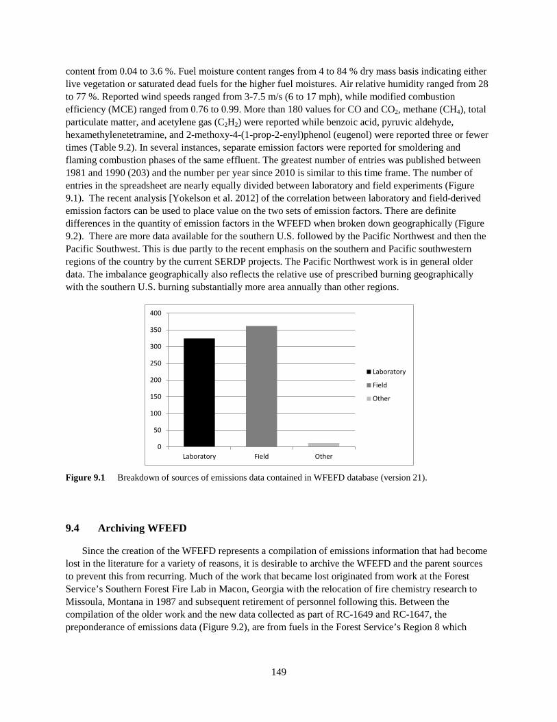
149
content from 0.04 to 3.6 %. Fuel moisture content ranges from 4 to 84 % dry mass basis indicating either live vegetation or saturated dead fuels for the higher fuel moistures. Air relative humidity ranged from 28 to 77 %. Reported wind speeds ranged from 3-7.5 m/s (6 to 17 mph), while modified combustion efficiency (MCE) ranged from 0.76 to 0.99. More than 180 values for CO and CO2, methane (CH4), total particulate matter, and acetylene gas (C2H2) were reported while benzoic acid, pyruvic aldehyde, hexamethylenetetramine, and 2-methoxy-4-(1-prop-2-enyl)phenol (eugenol) were reported three or fewer times (Table 9.2). In several instances, separate emission factors were reported for smoldering and flaming combustion phases of the same effluent. The greatest number of entries was published between 1981 and 1990 (203) and the number per year since 2010 is similar to this time frame. The number of entries in the spreadsheet are nearly equally divided between laboratory and field experiments (Figure 9.1). The recent analysis [Yokelson et al. 2012] of the correlation between laboratory and field-derived emission factors can be used to place value on the two sets of emission factors. There are definite differences in the quantity of emission factors in the WFEFD when broken down geographically (Figure 9.2). There are more data available for the southern U.S. followed by the Pacific Northwest and then the Pacific Southwest. This is due partly to the recent emphasis on the southern and Pacific southwestern regions of the country by the current SERDP projects. The Pacific Northwest work is in general older data. The imbalance geographically also reflects the relative use of prescribed burning geographically with the southern U.S. burning substantially more area annually than other regions.
Figure 9.1 Breakdown of sources of emissions data contained in WFEFD database (version 21).
9.4 Archiving WFEFD
Since the creation of the WFEFD represents a compilation of emissions information that had become lost in the literature for a variety of reasons, it is desirable to archive the WFEFD and the parent sources to prevent this from recurring. Much of the work that became lost originated from work at the Forest Service’s Southern Forest Fire Lab in Macon, Georgia with the relocation of fire chemistry research to Missoula, Montana in 1987 and subsequent retirement of personnel following this. Between the compilation of the older work and the new data collected as part of RC-1649 and RC-1647, the preponderance of emissions data (Figure 9.2), are from fuels in the Forest Service’s Region 8 which
0
50
100
150
200
250
300
350
400
Laboratory Field Other
Laboratory
Field
Other

150
covers the states south of the Mason-Dixon line from the Atlantic Ocean to the Big Thicket region of eastern Texas.
Figure 9.2 Emissions data distribution by U.S. Forest Service Regions, and Canada
Some of the key features that we wish the host site to have are: 1) longevity, 2) ease of use, and 3) ideally, that the potential users have some prior familiarity with the site. Regarding 1) longevity, it is clearly important that the web site will not simply vanish as a given program ends or as certain personnel move to other positions. This can seldom be guaranteed, but should be sought if possible. The second criterion is 2) ease of use. This criterion can be somewhat more difficult to define as each software, and software advocate, clearly emphasizes its pros but seldom its cons. In this instance it was also considered who the user clientele will be. While some individuals will be USFS employees, others will be DoD, many others will be state or local base managers and foresters. It was thus decided that any host or frame site should be as non-agency specific as possible, e.g. one that is open access.
After some consultation with potential users, specifically Dr. Roger Ottmar, it was first decided to consider the Fire Research and Management Exchange System (or FRAMES) web site to host the data (http://frames.gov, but the original site page is no longer active due to site migration). Dr. Ottmar considered this a particularly good choice as they (the USFS) are already using FRAMES to post their data from the RxCADRE burns. The goal of the web site is well aligned with overall project objectives of RC-1648 and RC-1649. From the web site: “The goal of FRAMES is to provide a systematic method of exchanging information and transferring technology between wildland fire researchers, managers, and other stakeholders in order to make wildland fire documents, data, tools, and other information resources easy to find, access, distribute, compare, and use.” Clearly this is what is desired in relation to this project. The FRAMES web site is also sponsored by several (long-term) agencies, including key USG agencies: the USFS, NPS, NBII, Joint Fire Science Program, BLM as well as the Universities of Montana and Idaho.
The FRAMES site allows both static and dynamic interaction and met all the criteria. An initial web site was developed (http://www.frames.gov/partner-sites/serdp/serdp-befd/). The WFEFD web site contains background information on the project, point of contact information, supporting literature metadata, and two downloadable formats of the WFEFD, a basic Microsoft Excel 20075 format and a 5 The use of trade names is provided for informational purposes only and does not constitute endorsement by the U.S. Department of Agriculture.

151
prototype GUI Microsoft Excel format (Figure 9.3). After concerns were raised at the 2012 IPR about FRAMES as the permanent host, additional sites were considered. While the FRAMES site continues to be active, the contract with FRAMES was discontinued; and the site is no longer being supported. An EPA repository was considered but is not currently being pursued due to the extensive quality assurance work that would have to be performed prior to the database being loaded onto the site. The QA work is not currently funded nor does it seem appropriate for a compilation of old data, most of which is no longer possible.
Figure 9.3 Screenshot of GUI Format of WFEFD.
The Forest Service data archive was therefore contacted as a potential host. The initial response from David Rugg, the Forest Service National Research Data Archivist indicated that this would be an appropriate repository. This site will accommodate downloading of the data for use by interested persons. Once the metadata are compiled for the database, it will be uploaded and made available as a citable database. In addition to the Excel spreadsheet, the data will be available in a comma-separated (.csv) format and copies of the original references will be provided in Adobe page description format (.pdf). The WFEFD has been submitted to the Forest Service archive where it is now being evaluated.
The FS Archives meets the outlined criteria, could be active quickly and has built-in security features that neither FRAMES or the EPA have. The FS Archives has three levels of security to choose from: 1) Open Access - data products have publicly available metadata documents and data that are readily accessible via the selected dissemination mechanism (e.g., download, optical media, on-line database). The Open Access—Data Use Agreement is anonymously agreed to by anyone acquiring data from this repository. 2) Monitored Access— data products have metadata documents that are publicly accessible, but users must agree to the Monitored Access - Data Use Agreement and register with the Forest Service before data are released. Data authors are provided with contact information for data users and planned use(s) of the data product. Collection of this information has been approved by OMB (Approval Number 0596-0210) in accordance with the Paperwork Reduction Act. 3) External— data products have publicly

152
available metadata documents through this archive. Data products are accessible via links to an external archive. The Monitored Access option would allow the designated point of contact to monitor who and how the WFEFD is being used. While the FS Archives is open to the public there is some concern that people outside of the U.S. Forest Service agency may not be familiar with it.
9.5 Literature Evaluated for Emissions Data
9.5.1 Database Literature Sources
Andreae, M. O. et al: Emission of Trace Gases and Aerosols from Biomass Burning, Global Biogeochemical Cycles, Vol. 15. No. 4: 955-966, 2001, DATABASE ID: 193
Babbitt, R.E. et al: Smoke From Western Wildfires, 1994, Proceedings of the 1994 Annual Meeting of Interior West Fire Council, 1994, DATABASE ID: 101
Bertschi, Isaac, et al: Trace Gas and Particle Emissions from Fires in Large-Diameter and Belowground Biomass Fuels, Journal of Geophysical Research, Vol. 108, No. D13, 8472, 2003, DATABASE ID: 121
Bovee, Harley et al: The Study of Forest Fire Atmospheric Pollution, USFS 4040 (4000) Interim Report 68-1, 1969, DATABASE ID: 4
Burling, I.R. et al: Laboratory Measurements of Trace Gas Emissions from Biomass Burning of Fuel Types from the Southeastern and Southwestern United States, Atmospheric Chemistry and Physics, Vol 10: 11115-11130, 2010, DATABASE ID: 172
Burling, I.R. et al: Airborne and Ground-based Measurements of the Trace Gases and Particles Emitted by Prescribed Fires in the United States, Atmospheric Chemistry and Physics, Vol 10: 12197-12216, 2011, DATABASE ID: 173
Chen, L.-W. A. et al: Emissions from Laboratory Combustion of Wildland Fuels: Emission Factors and Source Profiles, Environmental Science & Technology, Vol. 41, No. 12, 2007, DATABASE ID: 197
Chen, L.-W. A. et al: Moisture Effects on Carbon and Nitrogen Emission from Burning of Wildland Biomass, Atmospheric Chemistry and Physics Discussions, 10, 7985-8007, 2010, DATABASE ID: 182
Clements, Hubert B. et al: Nitrogen Oxides from Burning Forest Fuels Examined by Thermogravimetry and Evolved Gas Analysis, Thermochimica Acta, 35: 133-139, 1980, DATABASE ID: 144
Clements, Hubert B. et al: A Microcombustion Method to Measure Forest Fuel Emissions, Journal of Fire Sciences, VOL. 2: 260-275, 1984, DATABASE ID: 42
Fritschen, Leo et al: Slash Fire Atmospheric Pollution, USDA Forest Service Research Paper PNW-97, 1970, DATABASE ID: 150
Goode, Jon G. et al: Trace Gas Emissions from Laboratory Biomass Fires Measured by Open-Path Fourier Transform infrared Spectroscopy: Fires in Grass and Surface Fuels, Journal of Geophysical Research Vol. 104, No. D17: 21237-21245, 1999, DATABASE ID: 118

153
Goode, Jon G. et al: Measurements of Excess O3, CO2, CO, CH4, C2H4, C2H2, HCN, NO, NH3, HCOOH, CH3COOH, HCHO, and CH3OH in 1997, Journal of Geophysical Research, 2000, DATABASE ID: 119
Hardy, Colin C. et al: PM2.5 Emissions from a Major Wildfire using A GIS: Rectification of Airborne Measurements, Pacific Northwest International Section of the Air and Waste Management Association Annual Meeting, Bellevue, Washington, 1992, DATABASE ID: 87
Hays, Michael D. et al: Speciation of Gas-Phase and Fine Particle Emissions from Burning of Foliar Fuels, Environmental Science & Technology Vol. 36, No. 11, 2002, DATABASE ID: 143
Hegg, Dean et al: Emissions of Some Trace Gases From Biomass Fires, 82nd Annual Meeting and Exhibition Anaheim, California, 1989, DATABASE ID: 63
Hennigan, C. J. et al: Chemical and Physical Transformations of Organic Aerosol from the Photo-oxidation of Open Biomass Burning in an Environmental Chamber, Atmospheric Chemistry and Physics, 11, 7669-7686, 2011, DATABASE ID: 203
Laursen, Krista K. et al: Some Trace Gas Emissions from North American Biomass Fires with as Assessment of Regional and Global Fluxes from Biomass Burning, Journal of Geophysical Research Vol. 97, No.D18:20687-20701, 1992, DATABASE ID: 88
Long, Russell W. et al: Continuous Determination of Fine Particulate Matter Mass the Salt Lake City Environmental Monitoring Project: A Comparison of Real-Time and Conventional TEOM Monitor Result, Journal of the Air &Waste Management Association 55:1839-1846, 2005, DATABASE ID: 152
Mazzoleni, Lynn R. et al: Emissions of Levoglucosan, Methoxy Phenols, and Organic Acids from Prescribed Burns, Laboratory Combustion of Wildland Fuels, and Residential Wood Combustion, Environmental Science & Technology, Vol. 41, No. 7, 2007, DATABASE ID: 194
McKenzie, Lisa M. et al: Quantification of Major Components Emitted from Smoldering Combustion of Wood, Atmospheric Environment Vol. 28, No.20:3285-3292, 1994, DATABASE ID: 103
McKenzie, Lisa M. et al: Measurement and Modeling of Air Toxins from Smoldering Combustion of Biomass, Environmental Science & Technology, Vol. 29, No. 8 , 1995, DATABASE ID: 106
McMahon, Charles K. et al: Polynuclear Aromatic Hydrocarbons in Forest Fire Smoke, Carcinogenesis, Vol. 3 Polynuclear Aromatic Hydrocarbons, 1978, DATABASE ID: 146
McMahon, Charles K. et al: Characteristics of Forest Fuels, Fires and Emissions, 76th Annual Meeting of the Air Pollution Control Association, 1983, DATABASE ID: 39
McMeeking, Gavin R. et al: Emissions of Trace Gases and Aerosols During the Open Combustion of Biomass in the Laboratory, Journal of Geophysical Research D, Vol. 114 D19210, (2009)
Mickler, Robert A. , et al: Development and Demonstration of Smoke Plume, Fire Emissions, and Pre-and Post-prescribed Fire Models on North Carolina Coastal Plain Forest Ecosystems, The Fire

154
Environment Innovations, Management, and Policy, Conference Proceedings , 2007, DATABASE ID: 142
Nelson, Ralph M. et al: Backfire Particulate Emissions and Byram's Fire Intensity, Forest Service Note SE- 290, 1980, DATABASE ID: 26
Nelson, Ralph M. et al: Flame Characteristics for Fires in Southern Fuels, Forest Service Research Paper SE-205, 1990, DATABASE ID: 148
Nelson, Ralph M. et al: An Evaluation of the Carbon Balance Technique for Estimating Emission Factors and Fuel Consumption in Forest Fires, 72nd Annual Meeting of the Air Pollution Control Association, 1982, DATABASE ID: 130
Patterson, E. M. et al: Absorption Properties and Graphitic Carbon Emission Factors of Forest Fire Aerosols, Geophysical Research Letters, Vol. 13, No. 1: 129-132, 1986, DATABASE ID: 53
Radke, L. F. et al: Airborne Studies of Particles and Gases from Forest Fires, Journal of the Air Control Association, Vol. 28, No. 1, 1978, DATABASE ID: 154
Radke, L. F. et al: Airborne Measurements on Smokes from Biomass Burning, Aerosols and Climate, Eds. Peter V. Hobbs and M. Patrick McCormick, A. Deepak Publishing , 1988, DATABASE ID: 59
Radke, L. F. et al: Airborne Monitoring and Smoke Characterization of Prescribed Fires on Forest Lands in Western Washington and Oregon: Final Report, General Technical Report PNW-GTR-251, 1990, DATABASE ID: 149
Radke, L. F. et al: Airborne Observations of Biomass Fires, Final Report to the National Institute of Standards and Technology, 1990, DATABASE ID: 139
Radke, L. F. et al: Particulate and Trace Gas Emissions from Large Biomass Fires in North America, Global Biomass Burning: Atmospheric, Climate, and Biospheric Implications. Cambridge, Massachusetts: MIT Press, 1991, DATABASE ID: 80
Tangren, Charles D. et al: Scattering Coefficient and Particulate Matter Concentration in Forest Fire Smoke, Journal of the Air Pollution Control Association Vol. 32 No. 7, 1982, DATABASE ID: 132
Urbanski, Shawn P. et al: Chemical Composition of Wildland Fire Emissions, Chapter 4, Developments in Environmental Science, vol. 8: 79-107, 2009, DATABASE ID: 181
Ward, Darold E. et al: A Sampling System for Measuring Emissions from West Coast Prescribed Fire, Annual General Meeting Air Pollution Control Association, Pacific Northwest International Section, Vancouver, BC. 1982, DATABASE ID: 35
Ward, Darold E. et al: Laboratory Measurements of Carbonyl Sulfide and Total Sulfur Emissions from Open Burning of Forest Biomass, 75th Annual Meeting of the Air Pollution Control Associations, New Orleans, Louisiana , 1982, DATABASE ID: 36

155
Ward, Darold E. et al: Measurement of Smoke from Two Prescribed Fires in the Pacific Northwest, 75th Annual Meeting of the Air Pollution Control Associations, New Orleans, Louisiana, 1982, DATABASE ID: 37
Ward, Darold E. et al: Advances in the Characterization and Control of Emissions from Prescribed Fires, 77th Annual Meeting of the Air Pollution Control Association, San Francisco, California, 1984, DATABASE ID: 46
Ward, Darold E. et al: Emission Factors for Particles from Prescribed Fires By Region in the United States, APCA/EPA International Specialty Conference, San Francisco, California: pp. 372-386, 1988, DATABASE ID: 61
Ward, Darold E. et al: Emissions From Prescribed Burning of Chaparral, Annual Meeting of the Air and Waste Management Association, Anaheim, California, 1989, DATABASE ID: 66
Ward, Darold E. et al: Air Toxic Emissions from Burning of Biomass Globally- Preliminary Estimates, 85th Annual Meeting and Exhibition Air and Waste Management, Kansas City, Missouri, 1992, DATABASE ID: 91
Ward, Darold E. et al: Emission Factor Measurement for Two Fires in British Columbia Compared with Results for Oregon and Washington, Proceedings Pacific Northwest International Section of the Air and Waste Management Association Annual Meeting, Bellevue, Washington, 1992, DATABASE ID: 94
Ward, Tony J. et al: The Missoula Valley Semivolatile and Volatile Organic Compound Study: Seasonal Average Concentrations, Journal of the Air &Waste Management Association 55:1007-1013, 2005, DATABASE ID: 151
Weise, David R. et al: Burning California Chaparral- an Exploratory Study of Some Common Shrubs and Their Combustion Characteristics, International Journal Wildland Fire 1(3):153-158, 1991, DATABASE ID: 86
White, Jerry D. et al: Emission Rates of Carbon Monoxide, Particulate Matter, and Benzo(a)Pyrene from Prescribed Burning of Fine Southern Fuels, Southeastern Forest Experiment Station Research Note SE-346, 1987, DATABASE ID: 180
Yokelson, Robert J. et al: Open-Path Fourier Transform Infrared Studies of Large Scale Laboratory Biomass Fires, Journal of Geophysical Research Vol. 101, No. D15: 21067-2080, 1996, DATABASE ID: 112
Yokelson, Robert J. et al: Emissions of Formaldehyde, Acetic Acid, Methanol, and other Trace Gases from Biomass Fires in North Carolina Measured by Airborne Fourier Transform Infrared Spectroscopy, Journal of Geophysical Research, Vol. 104, No. D23: 30109-30125, 1999, DATABASE ID: 134
9.5.2 Additional Literature Evaluated
Achtemeier, G. L. et al: Measurements of Moisture in Smoldering Smoke and Implications for Fog, International Journal Wildland Fire, 15, 517-252, 2006, DATABASE ID: 210

156
Akagi, S. K. et al: Emission Factors for Open and Domestic Biomass Burning for Use in Atmospheric Models, Atmospheric Chemistry and Physics Discussions, 10, 2010, DATABASE ID: 202
Akagi, S. K. et al: Evolution of Trace Gases and Particles Emitted by a Chaparral Fire in California, Atmospheric Chemistry and Physics, 12, 1397-1424, 2012, DATABASE ID: 204
Akagi, S. K. et al: Measurements of Reactive Trace Gases and Variable O3 Formation Rates in Some South Carolina Biomass Burning Plumes, Atmospheric Chemistry and Physics Discussion, 12, 25255-25328, 2012, DATABASE ID: 228
Alvarado, M. J. et al: Formation of Ozone and Growth of Aerosols in Young Smoke Plumes from Biomass Burning: 1. Lagrangian Parcel Studies, Journal of Geophysical Research, Vol. 114, D09306, 2009, DATABASE ID: 211
Anderson, Iris C. et al: Enhanced Biogenic Emissions of Nitric Oxide and Nitrous Oxide Following Surface Biomass Burning, Journal of Geophysical Research, Vol. 93: p 3893-3898, 1988, DATABASE ID: 62
Bankston, C.P. et al: Aspects of the Mechanisms of Smoke Generation by Burning Materials, Combustion and Flame 41: 273-292 , 1981, DATABASE ID: 28
Bissonnette, Luc R. , et al: Lidar Remote Sensing in Atmospheric and Earth Sciences , Twenty-First International Laser Radar Conference, 2002, DATABASE ID: 122
Bond, T. C. et al: A Technology-based Global Inventory of Black and Organic Carbon Emissions from Combustion, Journal of Geophysical Research, Vol. 109, D14203, 2004, DATABASE ID: 212
Boubel, Richard W. et al: Emissions from Burning Grass Stubble and Straw , Journal of the Air Pollution Control Association, Vol. 19, No. 7, 1969, DATABASE ID: 3
Brown, Alexander L. et al: Chemical Analysis of Solids and Pyrolytic Vapors from Wildland Trees, Energy & Fuels, Vol. 17: p. 1022-1027, 2003, DATABASE ID: 157
Brown, James K. et al: Comparisons of Particulate Emissions and Smoke Impacts from Presettlement, Full Suppression, and Prescribed Natural Fire Periods in the Selway-Bitterroot Wilderness, Int. J. Wildland Fire 4(3): 143-155, 1994, DATABASE ID: 102
Burchard, John K. et al: Significance of Particulate Emissions, Journal of the Air Pollution Control Association Vol. 25, No. 2, 1975, DATABASE ID: 15
Campbell, J. et al: Pyrogenic Carbon Emission from a Large Wildfire in Oregon, United States, Journal of Geophysical Research, Vol. 112, G04014, 2007, DATABASE ID: 229
Carpenter, Alan B. et al: Leaf Burning as a Significant Source of Urban Air Pollution, Journal of the Air Pollution Control Association Vol. 27, No.6, 1977, DATABASE ID: 21

157
Carroll, John J. et al: The Dependence of Open Field Burning Emissions and Plume Concentrations on meteorology, Field Conditions and Ignition Technique, Atmospheric Environment Vol. 11: 1037-1050, 1977, DATABASE ID: 22
Carter, M. C. et al: Prescribed Burning and Productivity in Southern Pine Forests: A Review, Forest Ecology and Management, 191, 93-109, 2004, DATABASE ID: 230
Chen, L.-W. A. et al: Particle Emissions from Laboratory Combustion of Wildland Fuels: In situ Optical and Mass Measurements, Geophysical Research Letters, Vol. 33, L04803, 2006, DATABASE ID: 195
Christian, T.J. et al: Comprehensive Laboratory Measurements of Biomass-Burning Emissions: 1. Emissions from Indonesian, African and other fuels, Journal of Geophysical Research, Vol. 108, No.D23, 2003, DATABASE ID: 123
Christian, T.J. et al: Comprehensive Laboratory Measurements of Biomass-Burning Emissions: 2. First Intercomparison of Open-Path FTIR, PTR-MS, and GC-MS/FID/ECD, Journal of Geophysical Research Vol. 109, D02311, doi:10.1029/2003JD003874, 2004, DATABASE ID: 124
Cofer III, Wesley R. et al: Automated Analyzer for Aircraft Measurements of Atmospheric Methane and Total Hydrocarbons, Rev. Sci. Instrum., Vol. 52, No. 10, 1981, DATABASE ID: 29
Cofer III, Wesley R. et al: Particulate Emissions from a Mid-Latitude Prescribed Chaparral Fire, Journal of Geophysical Research, Vol. 93, No. D5: 5207-5212, 1988, DATABASE ID: 56
Cofer III, Wesley R. et al: Trace Gas Emissions from a Mid-Latitude Prescribed Chaparral Fire, Journal of Geophysical Research, Vol. 93, No. D2: 1653-1658, 1988, DATABASE ID: 57
Cofer III, Wesley R. et al: Trace Gas Emissions from Burning Florida Wetlands, Journal of Geophysical Research, VOL. 95, NO. D2: p 1865-1870, 1990, DATABASE ID: 183
Cofer III, Wesley R. et al: Crown Fire Emissions of CO2, CO, H2, CH4, and TNMHC from a Dense Jack Pine Boreal Forest Fire, Geophysical Research Letters, Vol. 25, No. 21, P3919, 1998, DATABASE ID: 213
Core, J.E. et al: Slash Burning Particulate Impact Analysis in Oregon's Willamette Valley, Nat. Council for Air and Stream Improvement Conference, 1979, DATABASE ID: 129
Daniels, Anders et al: Prediction of Air Pollution Concentrations from Agricultural Burning, 68th Annual Meeting of the Air Pollution Control Association, Boston, Massachusetts, 1975, DATABASE ID: 158
Darley, Ellis F. et al: Air Pollution from Forest and Agricultural Burning, Spring Meeting Western States Section, 1972, DATABASE ID: 6
Edgerton, S.A. et al: Estimates of Air Pollution from Backyard Burning, Journal of the Air Pollution Control Association Vol. 34, No. 6, 1984, DATABASE ID: 43

158
Edye, Leslle A. et al: Analysis of Condensates from Wood Smoke: Components Derived from Polysaccharides and Lignins, Environmental Science & Technology, Vol. 2, No.6, 1991, DATABASE ID: 75
EPA: Seminar Publication Pollution Control in the Forest Products Industry, Northwest Forestry Burning, Chapter 3, 1979, DATABASE ID: 23
Evans, John S. et al: An Inventory of Particulate Emissions from Open Sources, Journal of the Air Pollution Control Association, 1980, DATABASE ID: 25
Feldstein M. et al: The Contribution of the Open Burning of Land Clearing Debris to Air Pollution, Journal of the Air Pollution Contract Association Vol. 13, No. 11, 1963, DATABASE ID: 1
Ferguson, S.A. et al: Modeling Emissions for Prescribed Burning, 12th conference on Fire and Forest Meteorology, 1993, DATABASE ID: 135
Ferrare, Richard A. et al: Satellite Measurements of Large-Scale Air Pollution: Measurements of Forest Fire Smoke, Journal of Geophysical Research, Vol. 95, No.D7:9911-9925, 1990, DATABASE ID: 70
Franklin, Scott E. et al: Prescribed Fire in Southern California: Managing Conflicts of Public Safety and Air Quality, Air and Waste Management Association 8th Annual Meeting, 1989, DATABASE ID: 71
Gerstle, R.W. et al: Atmospheric Emissions From Open Burning, Journal of the Air Pollution Contract Association Vol. 17, No. 5, 1967, DATABASE ID: 2
Grieshop, A. P. et al: Laboratory Investigation of Photochemical Oxidation of Organic Aerosol from Wood Fires 2: Analysis of Aerosol Mass Spectrometer Data, Atmospheric Chemistry and Physics, 9, 2227-2240, 2009, DATABASE ID: 216
Griffith, David W. T, et al: FTIR Remote Sensing of Biomass Burning Emissions of CO₂, CO, CH4, CH2O, NO, NO2, NH3, and N2O, Global Biomass Burning: Atmospheric, Climatic, and Biospheric Implications, 1991, DATABASE ID: 74
Hall, J. Alfred et al: Forest Fuels, Prescribed Fire, And Air Quality, Pacific Northwest Forest and Range Experiment Station Forest Service, 1972, DATABASE ID: 7
Hao, Wei Min et al: Emissions of N2O from the Burning of Biomass in an Experimental System, Geophysical Research Letters, Vol. 18, 999-1002, 1991, DATABASE ID: 224
Hao, Wei Min et al: Emissions from Burning Forest Fuels: Development of a Model, Conversion of Utilization of Waste Materials, 1996, DATABASE ID: 109
Hardy, Colin C. et al: Emission Factors for Particulate Matter by Phase of Combustion from Prescribed Burning, Air Pollution Control Association Pacific Northwest International Section 1986 Annual meeting, 1986, DATABASE ID: 52

159
Hardy, Colin C. et al: Guidelines for Estimating Volume, Biomass, and Smoke Production for Piled Slash, General Technical Report Pacific Northwest Research Station: PNW-GTR-364, 1996, DATABASE ID: 160
Hardy, Colin C. et al: Smoke Emissions from Prescribed Burning of Southern California Chaparral, Research Paper Pacific Northwest Research Station: PNW-RP-486, 1996, DATABASE ID: 159
Hardy, Colin C. et al: A Database for Spatial Assessments of Fire Characteristics, Fuel Profiles and PM10 Emissions, Journal of Sustainable Forestry Vol. 11, No. 1/2, pp. 229-244, 2000, DATABASE ID: 125
Hartman, M.W. et al: Literature Review and Survey of Emissions from Residential Wood Combustion and their Impact, Research and Development Literature Review EPA A-600/2-85-047, 1985, DATABASE ID: 147
Hegg, Dean et al: Ammonia Emissions from Biomass Burning, Geophysical Research Letters, Vol. 15, No. 4: 335-337, 1988, DATABASE ID: 161
Hegg, Dean et al: Nitrogen and Sulfur Emissions from the Burning of Forest Products Near Large Urban Areas, Journal of Geophysical Research, Vol. 92, No. D12, 1987, DATABASE ID: 190
Hileman, Bette et al: Biomass Burning: Environment Hurt More than Thought, C&EN: March 26, 1990: 4-5, 1990, DATABASE ID: 73
Hosseini, S. et al: Particle Size Distributions from Laboratory-Scale Biomass Fires Using Fast Response Instruments, Atmospheric Chemistry and Physics, 10, 8065-8076, 2010, DATABASE ID: 217
Hudson, James G. et al: Water Nucleation Properties of Chaparral Fire Aerosol Particles, 82nd Annual Meeting and Exhibition Anaheim, California, 1989, DATABASE ID: 76
Jenkins, Bryan M. et al: Quantitative Assessment of Gaseous and Condensed Phase Emissions from Open Burning of Biomass in a Combustion Wind Tunnel, Global Biomass Burning: Atmospheric, Climatic, and Biospheric Implications , 1991, DATABASE ID: 77
Jenkins, Bryan M. et al: Wind Tunnel Modeling of Atmospheric Emission from Agricultural Burning: Influence of Operating Configuration on Flame Structure and Particle Emission Factor for a Spreading-Type fire, Environment Science Technology Vol. 27, No. 9, 1993, DATABASE ID: 95
Jenkins, Bryan M. et al: Emissions of Polycyclic Aromatic Hydrocarbons (PAH) from Biomass Burning, ACS 209th Annual National Meeting, 1995, DATABASE ID: 104
Jenkins, Bryan M. et al: Emission Factors for Polycyclic Aromatic Hydrocarbons from Biomass Burning, Environmental Science & Technology Vol. 30, No. 8: pp. 2462-2469, 1996, DATABASE ID: 178
Johnson, T. J. et al: An Infrared Spectral Database for Detection of Gases Emitted by Biomass Burning, Vibrational Spectroscopy, 53, 97-102, 2010, DATABASE ID: 218
Kasischke, E. S. et al: Influences of Boreal Fire Emissions on Northern Hemisphere Atmospheric Carbon and Carbon Monoxide, Global Biogeochemical Cycles. Vol. 19, GB1012, 2005, DATABASE ID: 214

160
Khalil, M.A.K. et al: Gaseous Tracers for Sources of Regional Scale Pollution, Journal of the Air Pollution Control Association, 1985, DATABASE ID: 48
Knight, J. A. et al: Characterization of Fuels and Products of Burning Experiments of Forestry Materials, Final Report Research Project Southern Forest Fire Laboratory No. A-1626, 1975, DATABASE ID: 201
Komarek, E.V. et al: The Ecology of Smoke Particulates and Charcoal Residues from Forest and Grassland Fires: A Preliminary ATLAS, Miscellaneous Publication No. 3, 1973, DATABASE ID: 9
Lahm, Peter W. et al: The Future of Prescribed Fire in the West Considering PM-10 Standards and Other Air Quality Programs, AWMA/EPA Specialty Conference PM-10 Standards and Non-Traditional Particulate Source Controls Session 3: Prescribed Burning in Agriculture and Land Management, , DATABASE ID: 137
Lamb, B. et al: Isoprene Emission Fluxes Determined by an Atmospheric Tracer Technique, Atmospheric Environmental Vol. 20, No. 1, pp. 1, 1986, DATABASE ID: 198
LeBel, P.J. et al: Nitric Acid and Ammonia Emissions From a Mid-Latitude Prescribed Wetlands Fire, Geophysical Research Letters, Vol. 15, No. 8: pp. 792-795, 1988, DATABASE ID: 162
Lee, Sangil et al: Gaseous and Particulate Emissions from Prescribed Burning in Georgia, Environmental Science & Technology Vol. 39, No 23: pp. 9049-9056, 2005, DATABASE ID: 179
Lee, Taehyoung, et al: Chemical Smoke Marker Emissions During Flaming and Smoldering Phase of Laboratory Open Burning of Wildland Fuels, Aerosol Science and Technology, 44: i-v, 2010, DATABASE ID: 208
Levin, E. J. T. et al: Biomass Burning Smoke Aerosol Properties Measured During Fire Laboratory at Missoula Experiments (FLAME), Journal of Geophysical Research, Vol. 115, D18210, 15 PP., 2010, DATABASE ID: 207
Levine, Joel S. et al: The Effects of Fire on Biogenic Soil Emissions of Nitric Oxide and Nitrous Oxide, Global Biogeochemical Cycles, Vol. 2. No. 4: 445-449, 1988, DATABASE ID: 58
Levine, Joel S. et al: The Effects of Fire on Biogenic Emissions of Methane and Nitric Oxide from Wetlands, Journal of Geophysical Research, Vol. 95, No.D2:1853-1864, 1990, DATABASE ID: 72
Levine, Joel S. et al: Biomass Burning A Driver for Global Change, Environmental Science & Technology Vol. 29, No. 3, 1995, DATABASE ID: 105
Lobert, J. M. et al: Importance of Biomass Burning in the Atmospheric Budgets of Nitrogen-containing Gases, Nature Vol. 346: pp. 552-554, 1990, DATABASE ID: 163
Lobert, J. M. et al: Experimental Evaluation of Biomass Burning Emissions: Nitrogen and Carbon Containing Compounds, Global Biomass Burning: Atmospheric, Climatic, and Biospheric Implications pp. 289-304, 1991, DATABASE ID: 164

161
Mack, L. A. et al: Optical Closure Experiments for Biomass Smoke Aerosols, Atmospheric Chemistry and Physics, 10, 9017-9026, 2010, DATABASE ID: 206
Mallory, William R. et al: Chemicals in Vapors of Smoldering Wood Fires, Forest Science Vol. 22, No.1: 81-83, 1976, DATABASE ID: 18
Mason, Sherri A. et al: Complex Effects Arising in Smoke Plume Simulations due to Inclusion of Direct Emissions of Oxygenated Organic Species from Biomass Combustion, Journal of Geophysical Research, Vol. 106, No.D12:12527-12539, 2001, DATABASE ID: 120
McMahon, Charles K. et al: Some Chemical and Physical Characteristics of Emissions from Forest Fires, Presented at 69th Annual Meeting of the Air Pollution Control Association, Portland, OR, 1976, DATABASE ID: 175
McMahon, Charles K. et al: Combustion Characteristics and Emissions from Burning Organic Soils, Presented at 73rd Annual Meeting of the Air Pollution Control Association, Montreal, Quebec, 1980, DATABASE ID: 176
McMahon, Charles K. et al: Combustion Process in Wildland Fuels Research Project, USDA Forest Service Southern Forest Fire Laboratory Research Progress Report 1980-1985, 1985, DATABASE ID: 145
McMahon, Charles K. et al: Organic Compounds in the Particulate Matter from Burning Organic Soils, Environmental Impacts of Natural Emissions, APCA Specialty Conference, South Atlantic Section Air Pollution Control Association, Research Triangle Park, NC, 1985, DATABASE ID: 49
Miller, P. et al: Shrubland Management Effects on Air Quality, Scrublands in California: Literature Review and Research Needed for Management, Chapter 10, 1984, DATABASE ID: 44
Montgomery, Tami A. et al: Continuous Infrared Analysis of N2O in Combustion Products, JAPCA Vol. 39, No. 5, 1989, DATABASE ID: 64
Naeher, Luke P. et al: Real-time and time-integrated PM2.5 and Co from Prescribed Burns in Chipped and Non-Chipped Plots: Firefighter and Community Exposure and Health Implications, Journal for Exposure Science and Environmental Epidemiology 16, 351-361, 2006, DATABASE ID: 177
Nance, David J. et al: Airborne Measurements of Gases and Particles from an Alaskan Wildfire, Journal of Geophysical Research Vol. 98, No.D8: 14873-14882, 1993, DATABASE ID: 155
Nelson, Ralph M. et al: An Evaluation of the Carbon Balance Technique for Estimating Emission Factors and Fuel Consumption in Forest Fires, 72nd Annual Meeting of the Air Pollution Control Association, 1982, DATABASE ID: 130
Nikolov, N. et al: Impact of Wildland Fires and Prescribed Burns on Ground Level Ozone Concentration, Review of Current Science Concepts and Analytical Approaches, NIFC, DATABASE ID: 220
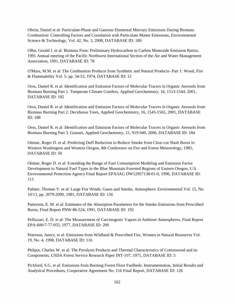
162
Obrist, Daniel et al: Particulate-Phase and Gaseous Elemental Mercury Emissions During Biomass Combustion: Controlling Factors and Correlation with Particulate Matter Emissions, Environmental Science & Technology, Vol. 42, No. 3, 2008, DATABASE ID: 189
Olbu, Gerald J. et al: Biomass Fires: Preliminary Hydrocarbon to Carbon Monoxide Emission Ratios, 1991 Annual meeting of the Pacific Northwest International Section of the Air and Water Management Association, 1991, DATABASE ID: 78
O'Mara, M.M. et al: The Combustion Products from Synthetic and Natural Products- Part 1: Wood, Fire & Flammability Vol. 5: pp. 34-53, 1974, DATABASE ID: 12
Oros, Daniel R. et al: Identification and Emission Factors of Molecular Tracers in Organic Aerosols from Biomass Burning Part 1. Temperate Climate Conifers, Applied Geochemistry, 16, 1513-1544, 2001, DATABASE ID: 185
Oros, Daniel R. et al: Identification and Emission Factors of Molecular Tracers in Organic Aerosols from Biomass Burning Part 2. Deciduous Trees, Applied Geochemistry, 16, 1545-1565, 2001, DATABASE ID: 188
Oros, Daniel R. et al: Identification and Emission Factors of Molecular Tracers in Organic Aerosols from Biomass Burning Part 3. Grasses, Applied Geochemistry, 21, 919-940, 2006, DATABASE ID: 184
Ottmar, Roger D. et al: Predicting Duff Reduction to Reduce Smoke from Clear-cut Slash Burns in Western Washington and Western Oregon, 8th Conference on Fire and Forest Meteorology, 1985, DATABASE ID: 50
Ottmar, Roger D. et al: Extending the Range of Fuel Consumption Modeling and Emission Factor Development to Natural Fuel Types in the Blue Mountain Forested Regions of Eastern Oregon, U.S. Environmental Protection Agency Final Report EPA/IAG DW12957138-01-0, 1996, DATABASE ID: 111
Palmer, Thomas Y. et al: Large Fire Winds, Gases and Smoke, Atmospheric Environmental Vol. 15, No. 10/11, pp. 2079-2090, 1981, DATABASE ID: 156
Patterson, E. M. et al: Estimates of the Absorption Parameters for the Smoke Emissions from Prescribed Burns, Final Report PNW-86-524, 1991, DATABASE ID: 192
Pellizzari, E. D. et al: The Measurement of Carcinogenic Vapors in Ambient Atmospheres, Final Report EPA-600/7-77-055, 1977, DATABASE ID: 200
Peterson, Janice, et al: Emissions from Wildland & Prescribed Fire, Women in Natural Resources Vol. 19, No. 4, 1998, DATABASE ID: 116
Philpot, Charles W. et al: The Pyrolysis Products and Thermal Characteristics of Cottonwood and its Components, USDA Forest Service Research Paper INT-107, 1971, DATABASE ID: 5
Pickford, S.G. et al: Emissions from Burning Forest Floor Fuelbeds: Instrumentation, Initial Results and Analytical Procedures, Cooperative Agreement No. 116 Final Report, DATABASE ID: 126
163
Prakash, C.B. et al: Studies on Air Emissions from the Combustion of Wood-Waste, Combustion Science and Technology Vol. 6:81-88, 1972, DATABASE ID: 8
Radke, L. F. et al: Hydrocarbon and Biomass Fuel Fire Field Tests, Proceedings of the Smoke/Obscurants Symposium XIV Vol. II CRDEC-CR-092, 1990, DATABASE ID: 127
Radke, L. F. et al: Prescriptions for Biomass Fire Smoke Reductions, 11th Conference on Fire and Forest Meteorology, 1991, DATABASE ID: 81
Rasmussen, R. A. et al: Carbonyl Sulfide and Carbon Disulfide from the Eruptions of Mount St. Helens, Science, Vol. 215, pp. 665 -667, 1982, DATABASE ID: 79
Real, E. et al: Processes Influencing Ozone Levels in Alaskan Forest Fire Plumes During Long-range Transport Over the North Atlantic, Journal of Geophysical Research, Vol. 112, D10S41, 2007, DATABASE ID: 221
Reid, J. S. et al: A Review of Biomass Burning Emissions Part II: Intensive Physical Properties of Biomass Burning Particles, Atmospheric Chemistry and Physics, 5, 799-825, 2005, DATABASE ID: 219
Reinhardt, Timothy E. et al: Factors Affecting Methyl Chloride Emissions from Forest Biomass Combustion, Environmental Science & Technology Vol. 29, No. 3, 1995, DATABASE ID: 107
Roberts, J. M. et al: Measurement of HONO, HNCO, and Other Inorganic Acids by Negative-ion Proton-transfer Chemical-ionization Mass Spectrometry (NI-PT-CIMS): Application to Biomass Burning Emissions, Atmospheric Measurement Techniques, 3, 981-990, 2010, DATABASE ID: 205
Robinson, Marin S. et al: Chemical Speciation of PM2.5 Collected During Prescribed Fires of the Coconino National Forest near Flagstaff, Arizona, Journal of the Air &Waste Management Association 54:1112-1123, 2004, DATABASE ID: 153
Sampson, R. Neil, et al: Wildfire and Carbon Emissions, 1993, DATABASE ID: 96
Sandberg, David V. et al: An Approach to Predicting Slash Fire Smoke, Tall Timber Fire Ecology Conference No. 15, Portland, OR, 1974, DATABASE ID: 13
Sandberg, David V. et al: Slash Fire Intensity and Smoke Emissions, Third National Conference on Fire and Forest meteorology of the American Meteorological Society and the Society of American Foresters, 1974, DATABASE ID: 11
Sandberg, David V. et al: Emissions From Slash Burning and The Influence of Flame Retardant Chemicals, Journal of the Air Pollution Control Association, Vol. 25, No. 3, 1975, DATABASE ID: 16
Sandberg, David V. et al: Effects of Fire on Air, National Fire Effects Workshop, 1978, DATABASE ID: 138
Sandberg, David V. et al: Air Quality Considerations in Using Prescribed Fire for Weed Control, John S. Wright Forestry Conference, Weed Control in Forest Management, Purdue University, 1981, DATABASE ID: 30

164
Sandberg, David V. et al: Air Quality Protection Aspects of Forestry Management, National Council of the Paper Industry for Air and Stream Improvement Technical Bulletin No. 390, 1982, DATABASE ID: 165
Sandberg, David V. et al: Research Leads to Less Smoke from Prescribed Fires, Northwest Forest Fire Council 1983 Annual Meeting, Olympia, WA, 1983, DATABASE ID: 166
Sandberg, David V. et al: Scheduling Prescribed Fires for Wetter Periods Reduces Air Pollutant Emissions, 8th Conference on Fire and Forest Meteorology, Society of American Foresters: pp. 132-138 , 1985, DATABASE ID: 51
Sandberg, David V. et al: Prescribed Fire Versus Air Quality in 2000 in the Pacific Northwest, General Technical Report PSW-101, presented at the Symposium on Wildland Fire 2000, Lake Tahoe, California, 1987, DATABASE ID: 55
Sandberg, David V. et al: Emission Reduction for Prescribed Burning, APCE/EPA International Specialty Conference: Transaction PM-10: Implementation of Standards, 1988, DATABASE ID: 40
Sandberg, David V. et al: Progress in Reducing Emissions from Prescribed Forest Burning in Western Washington and Western Oregon, Report Unknown, 1988, DATABASE ID: 60
Sandberg, David V. et al: Emissions Inventories for SIP Development, Report Unknown, Appendix D, August 15, 1997, 1997, DATABASE ID: 167
Sexton, Ken et al: Photochemical Ozone Formation in Urban and Point-Source Plumes, Environ. Sci. Technol.: 224-227, 1983, DATABASE ID: 41
Southerland, James H. et al: Emission Inventories and Air Quality Management, Air Pollution Control Association Specialty Meeting, 1982, DATABASE ID: 33
Spichtinger, N. et al: Boreal forest fires in 1997 and 1998: a Seasonal Comparison using Transport Model Simulations and Measurement Data, Atmospheric Chemistry and Physics, 4, 1857-1868, 2004, DATABASE ID: 215
Susott, Ronald A. et al: Fire Dynamics and Chemistry of Large Fires, Final Report Defense Nuclear Agency, IACRO 89-903, 1990, DATABASE ID: 140
Susott, Ronald A. et al: The Measurement of Trace Emissions and Combustion Characteristics for a Mass Fire, Global Biomass Burning: atmospheric, Climatic, and Biospheric Implications, 1991, DATABASE ID: 82
Tamanini, Francesco et al: A New Experimental Technique for Measuring the Burning Rate and Product Yield in Fire Plumes, Fall Technical Meeting, Eastern Section, The Combustion Institute, Princeton University, 1980, DATABASE ID: 133
Trentmann, J. et al: Chemical Processes in a Young Biomass-Burning Plume, Journal of Geophysical Research, Vol. 108, 4705, 2003, DATABASE ID: 222

165
Tsao, Rushung et al: Analysis of Smoke Aerosols from Nonflaming Combustion by Pyrolysis/Mass Spectrometry with Pattern Recognition , Analytical Chemistry, Vol. 56, No. 3, 1984, DATABASE ID: 45
Unknown, Emissions from Forestry Burning, Pollution Control in the Forest Products Industry, Chapter 3 Northwest Forestry Burning: pp. 7-10, 1979, DATABASE ID: 168
Verburg, P. et al: Nutrient Emissions from Prescribed Fire in the Lake Tahoe Basin: Implications from Field and Laboratory Observations, Desert Research Institute Report, 2009, DATABASE ID: 186
Veres, P. et al: Development and Validation of a Portable Gas Phase Standard Generation and Calibration System for Volatile Organic Compounds, Atmospheric Measurement Techniques, 3, 683-691, 2010, DATABASE ID: 226
Vose, James M. et al: Emissions from Forest Burning in the Southeastern United States: Application of a Model Determining Spatial and Temporal Fire Variation, Biomass Burning and Global Change Volume 2, The MIT Press, 1996, DATABASE ID: 196
Wade, Dale D. et al: An Analysis of the Air Force Bomb Range Fire, USDA Forest Service Research paper SE-105, 1973, DATABASE ID: 10
Waggoner, Alan P. et al: Airborne Observations of Emissions from the Clearwater Biomass Fires, 1992, DATABASE ID: 89
Waggoner, Alan P. et al: Airborne Observations of Emissions from the Clearwater Biomass Fires using Lidar, Pacific Northwest International Section of the Air and Waste Management Association Annual Meeting, 1992, DATABASE ID: 90
Walsh, George W. et al: Emission Standards of Particulates, Journal of the Air Pollution Control Association, Vol. 25, No. 2, 1975, DATABASE ID: 17
Ward, Darold E. et al: An Update on Particulate Emissions from Forest Fires, 69th Annual Meeting of the Air Pollution Control Association, Portland, Oregon, 1976, DATABASE ID: 20
Ward, Darold E. et al: Georgia Rural Air Quality: Effect of Agricultural and Forestry Burning, Journal of the Air Pollution Control Association, Vol. 26, No. 3, 1976, DATABASE ID: 19
Ward, Darold E. et al: Forest Fire Smoke Plume Documentation, 72nd Annual Meeting of the Air Pollution Control Association, Cincinnati, Ohio, 1979, DATABASE ID: 24
Ward, Darold E. et al: Particulate Matter Emission Factor Modeling For Fires in Southeastern Fuels, Sixth Conference Fire and Forest Meteorology Soc. Am. For., Seattle, Washington, 1980, DATABASE ID: 131
Ward, Darold E. et al: Particulate Matter Production from Cylindrical Laminar Diffusion Flames, Western States Section the Combustion Institute 1980 Fall Meeting, 1980, DATABASE ID: 27

166
Ward, Darold E. et al: Measurement of Smoke from Prescribed Fires in The Pacific Northwest, Annual General Meeting Air Pollution Control Association, Pacific Northwest International Section, Vancouver, BC, 1982, DATABASE ID: 34
Ward, Darold E. et al: Particulate Matter Emissions for Fires in the Palmetto-Gallberry Fuel Type, Forest Science Vol. 29, No. 4:761-770, 1982, DATABASE ID: 38
Ward, Darold E. et al: Source-Strength Modeling of Particulate Matter Emissions from Forest Fires, 76th Annual Meeting of the Air Pollution Control Association, Atlanta, GA, 1983, DATABASE ID: 169
Ward, Darold E. et al: Prescribed Fire Smoke Management Guide, National Wildfire Coordinating Group 420-1: Chapter II, 1985, DATABASE ID: 170
Ward, Darold E. et al: Characteristic Emissions of Smoke from Prescribed Fires for Source Apportionment, Air Pollution Control Association Pacific Northwest International Section 23rd Annual Meeting: pp. 160-167, 1986, DATABASE ID: 54
Ward, Darold E. et al: Air Toxic and Fireline Exposure, 10th Conference on Fire and Forest Meteorology, 1989, DATABASE ID: 69
Ward, Darold E. et al: Factors Influencing the Emissions of Gases and Particulate Matter from Biomass Burning, Third International Symposium of Fire Ecology, Freiburg University, Germany, 1989, DATABASE ID: 187
Ward, Darold E. et al: Organic and Elemental Profiles for Smoke from Prescribed Fires, Receptor Models in Air Resources management: Transaction of an International Specialty Conference of the Air & Waste Management Association 1988 Feb; San Francisco. Pittsburgh, Pennsylvania: Air & Waste Management Association: 299-321, 1989, DATABASE ID: 67
Ward, Darold E. et al: Factors Influencing the Emissions of Gases and Particulate Matter from Biomass Burning, Fire in the Tropical Biota, Ecological Studies, Vol. 84, 1990, DATABASE ID: 68
Ward, Darold E. et al: Field Characterization of Smoke Emissions from Biomass Fires Using Computer-Controlled Measurement Techniques, 11th Conference on Fire and Forest Meteorology, Missoula, Montana: p 494-502, 1991, DATABASE ID: 85
Ward, Darold E. et al: Managing Smoke and Maintaining Air Quality Standards, Course: Smoke Management, Lesson: Biomass Consumption and Emissions Production, 1991, DATABASE ID: 141
Ward, Darold E. et al: Projections of Emission From Burning of Biomass for Use in Studies of Global Climate and Atmospheric Chemistry, Annual Meeting of the Air and Waste Management Association, Vancouver, BC , 1991, DATABASE ID: 84
Ward, Darold E. et al: Smoke Emissions from Wildland Fires, Environmental International, Vol. 17: 117-134, 1991, DATABASE ID: 83

167
Ward, Darold E. et al: Characterization of the Combustion Process and Atmospheric Inputs from Biomass Burning: Global Scales, Fire in Pacific Northwest Ecosystems: Exploring Emerging Issues, 1992, DATABASE ID: 92
Ward, Darold E. et al: Emissions Measurement from Biomass Fires: A Comparative Evaluation of Methods and Results, Fire in the Environment: Its Ecological, Climatic and Atmospheric Chemical Importance, 1992, DATABASE ID: 93
Ward, Darold E. et al: An Inventory of Particulate Matter and Air Toxic Emissions from Prescribed Fires in the United States for 1989, Air and Waste Management Association 86th Annual Meeting, 1993, DATABASE ID: 65
Ward, Darold E. et al: Emissions Measurements from Vegetation Fires: A Comparative Evaluation of Methods and Results, Fire in the Environment: The Ecological, Atmospheric, and Climatic Importance of Vegetation Fires, 1993, DATABASE ID: 98
Ward, Darold E. et al: Particulate Matter and Air Toxic Emissions from Wildland Fires, Intermountain Research Station Report, 1993, DATABASE ID: 128
Ward, Darold E. et al: Particulate Matter and Trace Gas Emissions from the Canyon Creek Fire of 1988, 12th conference on Fire and Forest Meteorology, 1993, DATABASE ID: 99
Ward, Darold E. et al: Smoke Emissions from Ponderosa Pine Fuels Exposed to a Variety of Fire Histories and Site Preparation Treatments, USDA Forest Service Arizona Burns Final Report, 1993, DATABASE ID: 191
Ward, Darold E. et al: A Study of Emissions of Air Pollutants from Biomass Fires in the United States a Progress Report, 1995, DATABASE ID: 108
Ward, Darold E. et al: Progress in Smoke Characterization and Modeling, AIFM International Conference: Transboundary Pollution and the Sustainability of Tropical Forests: Towards Wise Forest Fire Management, 1996, DATABASE ID: 110
Ward, Darold E. et al: Review of Smoke Components, Health Hazards of Smoke Recommendations of the Consensus Conference, 5100 Fire, 1997, DATABASE ID: 199
Ward, Darold E. et al: Particulate Source Strength Determination for Low-Intensity Prescribed Fires, DATABASE ID: 209
Warneke, C. et al: VOC Identification and Inter-comparison from Laboratory Biomass Burning using PTR-MS and PIT-MS, International Journal of Mass Spectrometry, 303, 6-14, 2011, DATABASE ID: 225
Westerberg, H. et al: Hydrocarbon Production and Photochemical Ozone Formation in Forest Burn Plumes, Journal of the Air Pollution Control Association Vol. 31, No. 6, 1981, DATABASE ID: 31

168
White, Jerry D. et al: A Simplified Determination of Benzo[A]Pyrene in Particulate Matter from Prescribed Burning, USDA Forest Service Southern Forest Fire Laboratory Report, 1981, DATABASE ID: 32
White, Jerry D. et al: The Ratio of Benzo(A) Pyrene to Particulate Matter in Smoke from Prescribed Burning , EPA Proceedings: National Symposium on Recent Advances in Pollutant Monitoring of Ambient Air and Stationary Sources, 1984, DATABASE ID: 47
Worden, H. et al: Airborne Infrared Spectroscopy of 1994 Western Wildfires, Journal Unknown, 1994, DATABASE ID: 171
Yamate, George, et al: Emissions Inventory from Forest Wildfires, Forest Managed Burns, and Agricultural Burns, EPA-450/3-74-062, 1974, DATABASE ID: 14
Yokelson, Robert J. et al: An Evaluation of Some Trace Gas Measurement Strategies for Biomass Burning and the Resulting Recommendations, 1993, DATABASE ID: 100
Yokelson, Robert J. et al: Emissions from Smoldering Combustion of Biomass Measured by Open-Path Fourier Transform Infrared Spectroscopy , Journal of Geophysical Research Vol. 102, No. D15:18865-18977, 1997, DATABASE ID: 113
Yokelson, Robert J. et al: Smoke Chemistry Measurements by Airborne Fourier Transform Infrared Spectroscopy (AFTIR), IGAC International Symposium on Atmospheric Chemistry and Future Global Environment , 1997, DATABASE ID: 114
Yokelson, Robert J. et al: Trace Gas Emissions from Specific Biomass Fire-Types, START Synthesis Workshop on Greenhouse Gas Emission, Aerosols and Land Use and Cover Change in Southeast Asia , 1997, DATABASE ID: 115
Yokelson, Robert J. et al: Spectroscopic Studies of Biomass Fire Emissions, 13th Fire and Forest Meteorology Conference, 1998, DATABASE ID: 117
Yokelson, Robert J. et al: Evaluation of Adsorption Effects on Measurements of Ammonia, Acetic Acid, and Methanol, Journal of Geophysical Research, Vol. 108, 4649, 2003, DATABASE ID: 223
Yokelson, Robert J. et al: Coupling Field and Laboratory Measurements to Estimate the Emission Factors of Identified and Unidentified Trace Gases for Prescribed Fires, Atmospheric Chemistry and Physics Discussion, 12, 21517-21578, 2012, DATABASE ID: 227

169
10.0 Chapter 10
Biomass Burning Study at Fort Jackson: Atmospheric Emissions and the Effects of High Intensity Burns on Unmanaged Stands versus the Emissions from Fires Lit During the Wet
Season on Frequently Burned Stands6
10.1 Introduction
As described in Chapter 1, prescribed fires are necessary to help minimize the danger of wildfire, improve land access for training, improve forest health, and help maintain naturally occurring fire-adapted ecosystems. However, as detailed in Chapter 7, the emissions from prescribed fire can significantly impact local-regional air quality. The two main strategies to avoid smoke impacts are: (1) burning when the atmospheric conditions will both vigorously loft the emissions and direct them away from the populated areas, and (2) burning when the fuels are just dry enough to consume the desired amount of fuel (usually one to three days after rain), but before the site is so dry that large amounts of forest floor material smolder for prolonged periods, or worse yet, fire intensity damages the overstory.
Prolonged smoldering after convection from the site has ceased has been defined as “residual smoldering combustion” and is responsible for most of the negative air quality impacts of prescribed fire (e.g. smoke exposure complaints, visibility-limited highway accidents, etc.). Seldom do prescribed fires result in major damage to the overstory in what is termed (for most habitats) a stand replacement fire. [There are exceptions to this e.g. Florida scrub burns where stand replacement is the objective.] One case is the Cerro Grande fire near Los Alamos, New Mexico, where PF jumped the control lines during unexpected high winds in May 2000 and was finally controlled partly because it burned into an area where the fuel loads had been reduced by previous burning. Wildfires (WF), in contrast, normally burn when fire danger is at high levels and forest fuel moisture is at a minimum. This often results in significant amounts of RSC and/or stand-replacement fires. Wildfires are typically infrequent on any given site, but when they do occur, they often burn very large amounts of fuel and there are usually few or no options for reducing smoke impacts on populated areas. High fire danger is associated with high atmospheric pressure, which in turn may promote subsidence inversions and increased smoke impacts at the surface.
Despite the above-mentioned benefits of prescribed fires (PF), they can occasionally affect air quality, which needs to be recognized and understood. The possibility of unwanted impacts leads to strict regulation of PF (usually by county or state health authorities) and frequent questions by portions of the public as to their value. Such considerations make it appear unwise to oppose a careful, professionally-supervised PF program, but the justification is based largely on common sense and conventional wisdom, thus the long term trade-offs between the options are difficult to quantify. Even less understood is the potential for differences in the chemical composition of the smoke generated by prescribed- versus wild- 6 Much of the material in this chapter has already been reported as an open literature publication. Please see “Measurements of reactive trace gases and variable O3 formation rates in some South Carolina biomass burning plumes,” by Akagi, S. K., Yokelson, R. J., Burling, I. R., Meinardi, S., Simpson, I., Blake, D. R., McMeeking, G. R., Sullivan, A., Lee, T., Kreidenweis, S., Urbanski, S., Reardon, J., Griffith, D. W. T., Johnson, T. J. and Weise, D. R., Atmos. Chem. Phys., 13, 1141-1165, (2013).

170
fires. Given the above descriptions of how these fires behave, the question can be rephrased in more specific terms: “Is the smoke generated by RSC, high fuel loadings, or stand replacement fires chemically different from the smoke generated by lower intensity combustion of above-ground understory fuels at average loadings?” Many corollaries go with this question: If the smoke is different; does it evolve differently in the atmosphere or have different health (physiological) effects on the humans exposed to it?
This chapter describes a simple, three-prong research effort to further investigate the differences between WF and PF smoke chemistry and fuel consumption. In this research we investigated trace-gas emission factors from three pine-understory PFs in South Carolina conducted during the fall of 2011 that simulated high-intensity burns. During these experiments we looked at the differences in smoke emissions between fires occurring on land that is managed with frequent PF as opposed to higher intensity prescribed fires in stands with older fuels, i.e. on land where fire had not yet been reintroduced. The major features of this study were to expand the scope of measurements to include: (1) emissions data for fires that burned in forest stands with a broader range of management histories and additional important fuel types, (2) post-emission plume evolution data on days with different solar insolation and on a day with significant mixing of urban and fire emissions, and (3) addressing all these topics with a significantly expanded suite of instrumentation. The fuels included mature pine stands not previously subjected to PF and were lit following a period of sustained drought.
The suite of instruments was significantly expanded for the final field deployment reported in this chapter. The early Spring 2010 emissions data were produced by airborne and ground-based Fourier transform infrared spectrometers (AFTIR and LAFTIR, respectively) and an airborne nephelometer to estimate PM2.5 (particulate matter < 2.5 microns in diameter). In the work reported here, the trace gas measurements were supplemented by whole air sampling (WAS) on the ground and in the air, and an additional open-path FTIR spectrometer on the ground. Specifically, we report the first emission factor measurements made using a fixed open-path gas analyzer Fourier transform infrared (FTIR) system. We compared these emission factors with those obtained using a roving, point sampling, land-based FTIR and an airborne FTIR that were deployed on the same fires. We also compared to emission factors measured by a similar open-path FTIR system deployed on savanna fires in Africa. The particulate measurements featured a large suite of instruments to be described in detail in companion publications. In this chapter we report measurements obtained by AFTIR, LAFTIR, and WAS, which sampled trace gases in either well-lofted or initially unlofted emissions.
The previous pine-forest understory-fire measurements in this study (see Chapter 7) had been made in coastal North Carolina in February and March of 2010 after a prolonged period of high rainfall in intensively managed loblolly pine (Pinus taeda) and longleaf pine (Pinus palustris) stands. More specifically, the units had been treated with PF, mechanical fuel reduction, or logged within the last one to five years so that the understory reflected less than five years of re-growth. Through collaboration with the U.S. Army’s Fort Jackson in the Sandhills region of South Carolina, we were able to sample emissions from pine-forest understory fires in longleaf pine stands that had not been logged or burned by wild or prescribed fires in more than 50 years. The lower historical frequency of disturbance factors contributed to denser stands with relatively more hardwoods, litter, and shrubs in the understory fuels. Further, the fires reported here occurred during the Fall 2011 PF season, before the region had fully recovered from a prolonged summer drought. Thus, this study significantly increased the range of germane fuel and environmental conditions for which PF emissions have been measured. Extensive plume evolution data could not be acquired during the Camp Lejeune Spring 2010 PF measurements in pine-forest understory fires, due primarily to air-space restrictions. In contrast, in this study we had access

171
to the downwind plume for four of the seven fires and measured photochemical changes on one day with thick cloud cover and on three days with high solar insolation that included one day when the fire emissions mixed with the urban plume from the Columbia, South Carolina metropolitan area.
The data suggest that the method in which the smoke is sampled can strongly influence the relative abundance of the emissions that are observed. The airborne FTIR probed the bulk of the emissions, which were lofted in the convection column and the downwind chemistry, while the roving ground-based point sampling FTIR measured the contribution of individual residual smoldering combustion fuel elements scattered throughout the burn site. The open-path FTIR provided a ~30 m fixed path-integrated sample of emissions produced directly upwind mixed with emissions that were redirected by wind gusts, or right after ignition and before the adjacent plume achieved significant vertical development. It typically probed two distinct combustion regimes: “flaming-like” (immediately after adjacent ignition) and “smoldering-like”, denoted early and late, respectively. The calculated emission factors from open-path varied depending on the calculation method or from fire to fire given the changing MCE and dynamics over the duration of a typical burn. The emission factors from all three instruments can be plotted versus modified combustion efficiency for those chemical species that have emissions that are not highly fuel dependent (e.g. CH4 and CH3OH), and fit to a single consistent trend. The trend suggests that differences between the systems for these species may be mainly due to the unique mix of flaming and smoldering that each system sampled. For other more fuel-dependent species, the different fuels sampled also likely contributed to platform differences in emission factors. The path-integrated sample of the ground-level smoke layer adjacent to the fire provided by the open-path measurements is important as a first estimate for fire-line exposure to smoke for wildland fire personnel. We provide a table of estimated fire-line exposures for numerous known air toxics based on synthesizing results from several studies. Our data suggest that peak exposures are more likely to challenge permissible exposure limits for WF personnel than shift-average exposures.
One of the most interesting results (detailed later in this chapter) was the observation of monoterpenes produced by heating vegetative fuels during field fires. We report the first emission factors for a suite of monoterpenes, including the first quantitative FTIR observations of limonene in smoke along with an expanded suite of monoterpenes measured by WAS including α-pinene, β-pinene, limonene, camphene, 4-carene, and myrcene. The known chemistry of the monoterpenes and their measured abundance of 0.4-27.9% of non-methane organic compounds (NMOCs) and ~21% of organic aerosol (mass basis) suggests that they impacted secondary formation of O3, aerosols, and small organic trace gases such as methanol and formaldehyde in the sampled plumes in first few hours after emission. The variability in the initial terpene emissions in the South Carolina fire plumes was high and, in general, the speciation of the initially emitted gas-phase NMOCs was 13 to 195% different from that observed in a similar study in nominally similar pine forests in North Carolina ~20 months earlier. It is likely that differences in stand structure and environmental conditions contributed to the high variability observed within and between these studies. Other important results include the consistency of the ΔHCN/ΔCO emission ratio compared with previous airborne fire measurements in other coniferous-dominated ecosystems. The mean for these studies was 0.90±0.06%, further confirming the value of HCN as a biomass burning tracer. These results also support the finding that C3-C4 alkynes may be of use as biomass burning indicators on the time-scale of hours to a day. We also report the downwind chemical evolution of the plume on four of the fires and significant O3 formation (ΔO3/ΔCO from 10 to 90%) occurred in all of these plumes within two hours.

172
10.2 Site Descriptions
The three prescribed fires were conducted on 30 October, 1 November, and 2 November 2011 (referred to as Blocks 6, 9b, and 22b fires, respectively) and were located on the U.S. Army’s Fort Jackson base northeast of Columbia, South Carolina. Fort Jackson is located at 34.05o N latitude and -80.83o E and lies at the inner edge of the South Carolina coastal plain, approximately 175 km northwest from the Atlantic Ocean. Fort Jackson is in the Sandhills ecosystem, which supports a distinctive type of vegetation. The Sandhills form a belt that runs southwest to northeast across South Carolina of sands of varying depth with a high content of pure silica [Porcher and Rayner, 2001]. These deep sands support a distinctive type of vegetation, with the overstory vegetation described as a combination of two native southern pine species, namely longleaf pine (Pinus palustris) and loblolly pine (Pinus taeda), as well as turkey oak (Quercus laevis). In low density pine areas the understory has a diverse herbaceous layer with extensive wiregrass (Aristida sp.) and turkey oak regeneration. The longleaf pine-wiregrass subtype depends on fire, either natural or prescribed, for maintenance. The needle-litter and wiregrass can carry fire quite well and the mature longleaf pines are fire resistant. In high density pine areas associated with fire exclusion there is high degree of canopy closure, which results in less understory vegetation and relatively more duff/litter composed primarily of pine needles. Conversely, in the low density pine areas, there was sufficient sunlight to allow the understory growth of the turkey oak and other deciduous and herbaceous vegetation, mostly grasses. In Block 9b (burned on 1 November) there was significant growth of sparkleberry (Vaccinium arboreum) intermixed with the mature pine stands. Table 10.1 (partially reproduced from [Akagi et al., 2013]) provides fuels, weather, size, location, etc. for the seven PFs sampled in this study. As mentioned, Fort Jackson plots were specifically selected to include stands with significant understory growth, i.e. little or no recent prescribed burn history. The Sandhills vegetation community typically is burned every five to ten years to maintain forest health and also provide suitable army training grounds (www.dnr.sc.gov/cwcs/pdf/habitat/SandhillsHabitat.pdf), but the plots burned in this study were specifically selected to include stands with no recent PF (Blocks 6, 9b, and 22b, which had not been burned since 1957, 1956, and 2003, respectively). The burn plots, ignition sites and positions of the OPAG spectrometer are seen in Figure 10.1. Significant areas within Blocks 6 and 22b were dominated by hardwood vegetation typical of the Sandhills region. While Block 9f was exclusively natural longleaf pine, Block 22b also included a small drainage with the bottomland hardwood type (Figure 10.1). Forest type maps of the three blocks burned at Fort Jackson, South Carolina. Block 9b was principally longleaf pine while Block 6 and 22b contained significant quantities of scrub oak and other hardwood trees and understory typical of unburned longleaf pine stands. Note that the hardwood understory adjacent to the fire line in Figure 10.2. The older stand conditions at Fort Jackson, to some extent, serve as a living model of the fuel conditions expected if PF programs were further restricted across the South. Based on the fuel and fuel moisture conditions presented in Chapter 7, we can not conclude that the burns at Ft. Jackson were “higher intensity” burns that approached “wildfire” intensities. We can conclude that the fires were likely similar in behavior due to fuel moisture similarities. Both locations used firing patterns designed to burn the areas more quickly than would be burned with a single ignition source as would occur during a wildfire. While both sets of fires were prescribed, the Fort Jackson fires thus provide a contrast to the fires sampled earlier in this series of studies by Burling et al. [2011], which occurred on regularly burned sites during a wet spring.
173
Figure 10.1 Detailed burn maps of Block 6, Block 9b, and Block 22b PFs at Ft. Jackson. In upper panels, the
location of the OP-FTIR is shown as a blue circle, where fire was first lit shown by an orange circle. Fires were typically lit along firebreaks in a continuous line with the “fire origin” indicated by an orange dot representing where the fireline was initiated. Lower panel shows forest type maps.

174
Figure 10.2 Photos of understory vegetation typical of long-unburnt longleaf pine stands burned at Ft. Jackson in Nov 2011. Note the significant shrub
component and accumulated pine litter.
Table 10.1 Fire name, location, date, fuels description, size, atmospheric conditions, and burn history of fires sampled in this Ft. Jackson campaign.

175
10.3 Airborne Instrumentation
The airborne platform used was a USFS Region 4 Smoke-Jumpers Twin Otter N141Z, which had been customized with inlets, power, and racks for our research and was used successfully in our previous SERDP projects. The suite of airborne instruments was significantly expanded for the final field deployment reported here, making this one of the most detailed field studies of fire emissions to date. Airborne and ground-based instruments used at Fort Jackson are described in detail below.
10.3.1 Airborne Fourier Transform Infrared Spectrometer (AFTIR)
The main research instrument on the Twin Otter was the University of Montana (UM) airborne FTIR (AFTIR), which underwent major upgrades in 2008-2009 and performed well in the recently completed sampling of DoD PF at Camp Lejeune and elsewhere. The AFTIR was similar in concept to AFTIR instruments flown from 1997-2010 and has been previously described in Chapter 3 and Chapter 6. The FTIR was operated at a spectral resolution of 0.67 cm-1 (slightly lower than 0.5 cm-1 used previously) and four spectra were co-added every 1.5 seconds with a duty cycle > 95%. The f-matched exit beam from the FTIR was directed into a closed-path doubled White cell (IR Analysis, Inc.) permanently aligned at 78 m. The exit beam from the cell was focused onto a mercury cadmium telluride (MCT) detector. A forward-facing halocarbon wax coated inlet 25 mm opening 30 cm above the top of the leading edge of the aircraft cabin ceiling directed ram air into a 25 mm diameter perfluoroalkoxy (PFA) tube coupled to the White cell. The noise level for the four co-added spectra was 4 × 10⁻⁴ absorbance units, which allowed CO and CH4 to be measured in near “real time” with about 3-5 ppb peak-to-peak noise. Peak-to-peak noise for CO2 operating in this manner was about 1 ppm. The temporal resolution with the valves open was limited by the cell 1/e exchange time of about 5-10 s at typical Twin Otter sampling speeds of ~40-80 m s-1. Fast-acting, electronically activated valves located at the cell inlet and outlet allowed flow through the cell to be temporarily halted so that more scans of grab samples could be averaged to increase spectrometer sensitivity. Averaging ~100 scans (150 s) of a “grab sample” reduced peak-to-peak noise to 3 × 10⁻⁵ absorbance units, providing, for example, a methanol detection limit better than ~400 pptv (SNR = 1). At times we averaged scans obtained with the control valves open, which gave SNRs dependent on the time to transect the plume. AFTIR sensitivity is also impacted by interference from water vapor, which is highly variable. In general, due in large part to this project, the sensitivity has improved up to a factor of ~30× depending on the spectral region, since the first prototype AFTIR system was flown in 1997 to 2006. Detection limits for the compounds we report other than CO2 (see below) ranged from hundreds of ppt to 10 ppb for NO and NO2, where the gain in SNR was partially canceled by the decreased resolution.
The averaged sample spectra were analyzed either directly as single-beam spectra, or as transmission spectra referenced to an appropriate background spectrum, via multi-component fits to selected frequency regions with a synthetic calibration non-linear least-squares method (Chapter 4) As an exception to the fitting process, NO and NO2 only were analyzed by integration of selected peaks in the absorbance spectra. In all, the following gases were quantified and accounted for most of the features observed in the smoke spectra: water vapor (H2O), carbon dioxide (CO2), carbon monoxide (CO), methane (CH4), nitric oxide (NO), nitrogen dioxide (NO2), ammonia (NH3), hydrogen cyanide (HCN), nitrous acid (HONO), peroxyacetyl nitrate (PAN, CH3C(O)OONO2), ozone (O3), glycolaldehyde (HOCH2CHO), ethylene (C2H4), acetylene (C2H2), propylene (C3H6), limonene (C10H16), formaldehyde (HCHO), 1,3-butadiene (C4H6), methanol (CH3OH), furan (C4H4O), phenol (C6H5OH), acetic acid (CH3COOH), and formic acid

176
(HCOOH). Spectra were analyzed in regions of typically 10-200 cm-1 width, with each region targeting one or more trace gases. Table 10.1 summarizes all species reported and the spectral analysis regions from which they were retrieved. Typical precision (repeatability) of measurements is < 1% for dominant species such as CO2, CO and CH4, but accuracy may be a few percent, varying from species to species; Smith et al. (2011) provide a detailed analysis of the accuracy of OP-FTIR measurements. Detection limits for trace species are typically 1-10 ppb. Since all species are retrieved from the same spectrum at the same time, emission ratios can be determined for any pair of species at each spectrum time step (usually ~134 s). For NH3 only, we corrected for losses on the cell walls as described in Yokelson et al. [2003a].Excess mixing ratios for any species X in the plumes (denoted ΔX, the mixing ratio of species X in a plume minus its mixing ratio in background air measured before the fire) were obtained directly from the transmission spectra or by difference between the appropriate single beam retrievals for H2O, CO2, CO, and CH4 in the plume and pre-fire.
10.3.2 Whole Air Sampling (WAS) Canisters
WAS canisters were filled both from the Twin Otter and on the ground to measure an extensive suite of gases, mostly non-methane organic compounds (NMOCs). Sampling was manually controlled and the evacuated canisters were filled to ambient pressure in ~10-20 s in background air or in various smoke plumes. In the aircraft, the canisters were filled directly from the AFTIR multipass cell via a dedicated PFA valve and connecting tube after the IR signal averaging was complete. On the ground, the WAS samples were obtained in more dilute portions of the plumes than sampled by LAFTIR since the subsequent pre-concentration step could otherwise cause a non-linear detector response [Hanst et al., 1975; Simpson et al., 2011]. We collected four WAS canisters from the ground and four from the air (one background and three smoke samples per platform per fire) on each of the first three fires (Block 6, Block 9b, and Block 22b). All 24 canisters were sent to UC-Irvine for immediate analysis of 89 gases: CO2, CH4, CO, carbonyl sulfide (OCS), dimethyl sulfide (DMS), and 83 NMOCs by gas chromatography (GC) coupled with flame ionization detection (FID), electron capture detection (ECD), and quadrupole mass spectrometer detection (MSD). Every peak of interest on every chromatogram was individually inspected and manually integrated. The GC run times were extended to target quantification of limonene. Other prominent peaks in the chromatograms were observed, assigned, and quantified for species not in the suite of compounds usually analyzed by UC-Irvine, including 2-propenal, 2-methylfuran and butanone.
10.3.3 Other Airborne Measurements
In addition to the AFTIR and WAS measurements, there were several other airborne instruments including a single particle soot photometer (SP2) for measurement of refractory black carbon at STP (rBC, μg sm-3, 273 K, 1 atm) [Stephens et al., 2003], a particle-into-liquid sampler-total organic carbon [PILS-TOC, Weber et al., 2001] analyzer to detect water-soluble organic carbon (WSOC), and a high resolution time-of-flight (HR-ToF) aerosol mass spectrometer (AMS) to measure the mass concentration (μg sm-3) for the major non-refractory particle species including organic aerosol (OA), non-sea salt chloride, nitrate, sulfate, and ammonium. Measurements of aircraft position, wind velocity, temperature, relative humidity, and barometric pressure at 1-Hz were obtained with a wing-mounted Aircraft Integrated Meteorological Measuring System probe (AIMMS-20, Aventech Research, Inc.) [Beswick et al., 2008]. A Picarro cavity ring-down spectrometer measured H2O, CO2, CO, and CH4 at 0.5 Hz during flight. Ratioing the particle data to the Picarro CO measurements allowed synthesis of the particle data with the AFTIR and WAS trace gas measurements on the aircraft.

177
10.4 Ground-based Instrumentation:
10.4.1 Land-based Fourier Transform Infrared Spectrometer (LAFTIR)
Ground-based FTIR measurements are important for capturing point sources of residual smoldering combustion (RSC) smoke. In addition to WAS canisters, measurements of ground-based smoke were made using a battery-powered FTIR system [Christian et al., 2007] that can be wheeled across difficult terrain to sample remote sites. The vibration-isolated LAFTIR optical bench holds a MIDAC 2500 spectrometer, an MCT detector, and a White cell (Infrared Analysis, Inc.) aligned at 11.35 m pathlength. Sample air was drawn into the cell by an onboard pump through several meters of 1/4-inch PFA tubing. Two manual PFA shutoff valves allowed trapping of the sample in the cell to collect signal averaged spectra. Temperature and pressure inside the White cell were monitored and logged in real time on the on-board system laptop. Several upgrades to the FTIR originally described by Christian et al. [2007] included improvements to the electronics, source optics, and the data acquisition software (Essential FTIR, http://www.essentialftir.com/index.html). The LAFTIR was operated at 0.50 cm-1 and three scans were co-added every 1.15 seconds (with a duty cycle of about 38%). Smoke or background samples were typically held in the cell for several minutes while ~100-200 spectra were collected at ~1 Hz. The spectral quantification method was similar to that used in the AFTIR analysis. Signal averaged, grab sample, single beam spectra were analyzed directly for H2O, CO2, CO, and CH4 and referenced to appropriate background spectra to analyze for the following gases: NH3, HCN, C2H2, C2H4, C3H6, HCHO, CH3OH, CH3COOH, C6H5OH, C4H4O, C10H16, and C4H6. We corrected for NH3 losses on the White cell walls during storage, which increased the LAFTIR NH3 retrievals in this study by about 40% on average. Due mostly to a shorter pathlength (compared to the AFTIR system, see previous section), the LAFTIR detection limits ranged from ~50-200 ppb for most gases. This was sufficient for detection of many species since much higher concentrations were sampled on the ground than in the lofted smoke. Comparisons to the NIST-traceable standards for CO, CO2, and high levels of CH4 were usually within 1 to 2%. Background level calibrations for CH4 had weaker signals and up to 6% uncertainty, but that does not introduce significant error into the excess amounts in most cases. Several compounds observed by the AFTIR system (formic acid, glycolaldehyde, PAN, O3, NO, NO2, and HONO) were below the detection limits of the ground-based system. Finally, in several LAFTIR spectra a prominent peak was seen at 882.5 cm-1 that we could not assign.
10.4.2 Open-path FTIR Spectrometer (OP-FTIR)
The measurements of unlofted smoke were also made using a Bruker OPAG-22 open-path Fourier transform infrared spectrometer (Figure 10.3), This instrument provided a key asset in sampling smoke that was neither the lofted (flaming) smoke as sampled from the aircraft, nor from an individual flaming entity (stump, tree) on the ground, but rather sampled a mixture of both flaming and smoldering smoke along the fire line, similar to what a firefighter may experience. These results are described below.
The OPAG-22 is a tripod-mounted, field-portable FTIR system that can be used to record passive or active infrared absorption spectra through the atmosphere or gas plumes at distances across distances on the order of tens to hundreds of meters. In the present configuration at Fort Jackson it was used in an active configuration with an unmodulated SiC glowbar source and sender telescope at one end of the light path and the FTIR-telescope system at the other. This type of configuration with a remotely located source is often termed bistatic. The source was powered (~20 W) using a 12.6 V DC automobile battery.

178
Overnight charging was sufficient to run the system the following day for the duration of the fire. The source brightness temperature was approximately 1200 °C. The SiC source was mounted at the focal point of an f/4 Newtonian telescope with a 150 mm (6 inch) clear aperture. The telescope projected a collimated, broadband IR beam to a 150 mm receiver telescope coupled to the OPAG-22 spectrometer. Path lengths of 29.3-32.2 m were used to optimize infrared intensity and pathlength Figure 10.3b. The OP-FTIR was located on the portion of the fireline and measured smoke associated initially with the backing fires used to create the “black line” buffers commonly used in prescribed fires (Waldrop and Goodrick, 2012).
On the receiving end, the OPAG spectrometer is powered by two large automobile batteries ganged in serial to provide ~24 Volts DC; the power consumption is 40 W. The spectrometer's normal field of view is 30 milliradians but was reduced to 10 mrad via the use of 150 mm 3:1 reducing telescope attached to the OPAG entrance window (Figure 10.3a). The instrument has an optical throughput of 0.0082 steradian cm2 and f/# of 0.9. It has an AR-coated zinc selenide entrance window, a zinc selenide beamsplitter, and uses a closed cycle, cryogenically-cooled MCT as its IR detector. The detector uses a proprietary software correction for detector nonlinearity [Keens]. The spectrometer's interferometer uses dual retroreflecting cube corner mirrors in an inverted pendulum mechanism. This allows for a rugged interferometer that is not prone to wear and does have to be constantly realigned, and is relatively field-rugged as the interferometer moves entirely about its center of mass, thus less susceptible to jolt along the drive axis.
Figure 10.3 (a) Photograph of the OPAG-22 spectrometer and receiver telescope in the field. (b) Photograph of
sender and receiver telescopes separated by an optical path of ~30 m.
The instrument's maximum resolution is 0.5 cm-1 and can record eight spectra/second at a resolution of 4 cm-1 using the MCT detector. Its noise equivalent ΔT is, for a single spectrum, 0.02 K at 1000 cm-1 with a background temperature of 30 C. The instrument's noise equivalent radiance for a single spectrum is 0.033 mW/(m2 steradian cm-1) at 30 C and 1000 cm-1. The OPAG 22 is also equipped with two internal blackbodies that can be moved in front of the instrument's entrance window, but these were not used. Instead, after aligning the two telescopes, an external blackbody was placed in front of the sender telescope to record a blackbody spectrum each day. Spectra were recorded at a resolution of 1.5 cm-1 using double-sided forward-backward interferograms at 35 kHz modulation velocity. Data were collected for approximately 134 s per spectrum (50 co-added scans) to increase the signal-to-noise ratio. This typically allowed two or three spectra during the strong flaming phase. After aligning the telescopes, an ambient emission spectrum was recorded with the source turned off. This spectrum accounts for emission from the ambient-temperature environment which is modulated by the interferometer and detected in the FTIR spectra, and was subtracted from all measured glow bar spectra before analysis. After collection, data were Fourier transformed using the Mertz phase correction with boxcar (i.e. no) apodization.

179
Ratioing to background was used only in spectral regions where the continuum spectrum of the source-telescope-interferometer system was complex and could not be well fitted by the analysis procedure. The background spectrum was also used to characterize the composition of the pre-fire atmosphere. Analysis of the OPAG spectra was by iterative non-linear least-squares fitting of the measured spectra by calculated spectra as described in previous work [Griffith, 1996; Yokelson et al., 2007a; Burling et al., 2011, Griffith et al., 2012]. The calculated spectra are based on HITRAN [Rothman et al., 2009] and Pacific Northwest National Laboratory [Sharpe et al. 2004; Johnson et al., 2006, 2010] spectral databases, and include the effects of environmental pressure and temperature as well as the instrument lineshape and resolution.
10.5 Calculation of Excess Mixing Ratios, Normalized Excess Mixing Ratios (NEMRs), Emission Ratios (ERs), and Emission Factors (EFs)
Excess mixing ratios for FTIR species were calculated following the procedure in Chapter 6. Excess mixing ratios for WAS species were obtained by subtracting WAS background values from plume values. The normalized excess mixing ratio (NEMR) is calculated for all instruments by dividing ΔX by the excess mixing ratio of a long lived plume tracer ΔY, usually ΔCO or ΔCO2, measured in the same sample. The NEMR can be measured anywhere in the plume. NEMRs collected at the source of a fire are equivalent to an initial molar emission ratio (ER) at the time of measurement. ER have two important uses: (1) since the CO or CO2 tracers dilute at the same rate as the other species, differences between the ERs and the NEMRs measured downwind can sometimes help quantify post-emission chemical changes. (2) The ER can be used to calculate emission factors (EFs). Details of these two uses are described below.
In this study, downwind data were only collected in the aircraft and the ER obtained while the aircraft was sampling the source did not follow clear, time-dependent trends. Thus we combined all the source samples from each fire to compute a single fire-averaged initial emission ratio (and 1-σ standard deviation) for each fire. The fire-averaged ER were subsequently used both to calculate fire-averaged EF and as our best estimate of the starting conditions in the plumes. We computed the fire-averaged ERs from the slope of the linear least-squares line with the intercept forced to zero when plotting ΔX against ΔY for all X/Y pairs from the fire. The intercept is forced to zero because the background concentration is typically well known and variability in the plume can affect the slope and intercept if the intercept is not forced. This method heavily weights the large excess mixing ratios that may reflect higher rates of fuel consumption and data that have higher signal-to-noise. FTIR and WAS excess mixing ratios were combined in the calculation of ERs if a species was measured by both techniques.
For any carbonaceous fuel, source ERs can be used to calculate emission factors (EFs), which are expressed as grams of compound emitted per kilogram of biomass burned (on a dry weight basis). This procedure was detailed earlier in Chapter 6. This method is most accurate when the mass fraction of carbon in the fuel is precisely known and all the burnt carbon is volatilized and detected. Based on literature values for similar fuels [Susott et al., 1996; see Ch. 6] we assumed a carbon fraction of 0.50 by mass on a dry weight basis for fuels burned in this campaign. The actual fuel carbon fraction was likely within 5 to 10% of this value. Note that EFs scale linearly with the assumed fuel carbon fraction. Total emitted carbon in this study was determined from the sum of the carbon from AFTIR species and WAS species. This sum could underestimate the actual total carbon by 1 to 2% due to unmeasured carbon, which would lead to a slight, across-the-board overestimate of our calculated EFs of 1 to 2% [Akagi et al., 2011].

180
10.6 Airborne and Ground-based Sampling Approach
The Fort Jackson prescribed burns (Blocks 6, 9b, and 22b) were part of a collaboration with the forestry staff at the base. The LAFTIR ground-based sampling protocol was similar to that described in Chapter 7. Background samples were acquired before the fire and the burns were ignited in the late morning or early afternoon. Ground-based sampling access was sometimes precluded during ignition, but sampling access then continued through late afternoon until each fire was effectively out. During post-ignition access, numerous point sources of residual smoldering combustion (RSC) smoke were sampled by the mobile LAFTIR system minutes to hours after passage of a flame front. The spot sources of white smoke, mainly produced from pure smoldering combustion, included smoldering stumps, fallen logs, litter layers, etc., and they contributed to a dense smoke layer usually confined below the canopy. Point sources were usually sampled repeatedly to quantify their variability. Four WAS canisters were collected on the ground for each Fort Jackson fire (one WAS canister was always collected prior to ignition as a background along with three sampled RSC point sources, also sampled by LAFTIR system). Table 10.2 shows the RSC fuel types sampled on the ground for the Fort Jackson fires and Figure 10.4 shows two of these fuels.
Fuel Type # of Sites # of LAFTIR Samples # of WAS Samples
Dead/down debris 8 13 3 Stump 4 4 2
Live tree base 2 5 - Litter 4 4 -
Fatwood 2 6 1 Slash pile 1 4 -
Table 10.2 Ground-based fuels sampled by LAFTIR and WAS from Blocks 6, 9b, and 22b at Fort Jackson, SC.
Figure 10.4 Photographs of two examples of the fuels that contributed to residual smoldering combustion
emissions that were sampled by ground-based FTIR and WAS: (a) a live tree base, and (b) dead/down debris.
For the airborne measurements, mid-morning take-offs enabled us to sample the pre-fire background and then the initial emissions and adjacent backgrounds for as long as the fire produced a convection column that exceeded several hundred meters in height. To measure the initial emissions from the fires,

181
we sampled smoke less than several minutes old by penetrating the smoke column 150 to several thousand meters from the flame front. The goal was to sample smoke that had already cooled to the ambient temperature since any chemical changes associated with smoke cooling are not explicitly included in most atmospheric models. This approach also sampled smoke before most photochemical processing, which is explicitly included in most models. Afternoon flights were conducted to complete sampling of the initial emissions if necessary and to search for and sample the downwind plume (Figure 10.5, Figure 10.6, Figure 10.7).
Figure 10.5 Overview of all flight tracks for the Twin Otter aircraft. “RF” indicates research flight. Flight dates are
shown in Table 10.3 except for RF06, which sampled urban emissions. “Hotspots” are MODIS thermal anomalies from 30 October to 10 November Of the seven fires sampled in this study, only the pine plantation fire was detected as a satellite hotspot. Due to a GPS malfunction, the 10 November flight track is at 2-min resolution.

182
Figure 10.6 Detailed flight tracks and AFTIR downwind sample locations during RF03 (pink) and RF04 (brown),
which sampled the Block 9b fire at Fort Jackson on 1 November 2011. (The hotspot that appears to intersect RF03 is actually from the pine plantation fire sampled on 2 November)
Figure 10.7 Detailed flight tracks and AFTIR downwind sample locations during RF07 (red) and RF08 (black) on
7 and 8 Nov, sampling the Georgetown and Francis Marion fires, respectively.

183
The plumes diluted rapidly mostly in the top half of a somewhat hazy boundary layer due to variable winds (mixed layer extended to ~1100 m above mean sea level (a.m.s.l.)). Thus, of the Fort Jackson fires, it was only possible to locate the downwind plume and obtain quality downwind data on the Block 9b fire (1 Nov, research flights number 3 and 4; RF03 and RF04 in Figure 10.6, respectively). The prevailing winds on 1 November directed the plume through the Columbia metropolitan area and directly over an airport and a natural gas power plant; thus mixing of burn smoke with fossil fuel emissions was unavoidable. The plume from the Block 22b fire directly entered a large restricted area and could not be subsequently re-sampled. However, while searching for the downwind plume we located a fire on a pine plantation about 40 km south of Columbia (Table 10.1). The pine plantation fire generated a Geostationary Satellite System (GOES) hotspot from 13:02:00-17:15:00 LT, so our samples at ~16:42 LT were collected towards the end of this fire. This was the only fire in this study detected as a hotspot by GOES or Moderate Resolution Imaging Spectroradiometer (MODIS) satellites.
After the burns at Fort Jackson, we sampled additional fires throughout South Carolina on 7, 8, and 10 November (Georgetown, Francis Marion, and Bamberg Fires, respectively). Due to transit time the Twin Otter typically arrived after the fire had been in progress for 0.5 to 1.0 hours (ground-based sampling was not feasible due to long travel times and short notice). The airborne sampling of these fires initially focused on the source emissions. After ~1-1.5 hours of repeatedly sampling the source, we would then cross the plume at increasingly large downwind distances until it could not be differentiated from background air. We then repeated the crossing pattern in reverse order or returned directly to the source approximately along the plume center-line depending on conditions (Figure 10.7). The plumes from these three fires also diluted rapidly in the boundary layer to form broad “cone-shaped” plumes under the influence of light and variable winds. Estimated times since emission, or smoke ages, were calculated for all the downwind samples by first calculating the average wind speed from the AIMMS-20 for incremental altitude bins of 100 m a.m.s.l. The smoke sample distance from the plume source was then divided by the average wind speed at the sample altitude, as shown in Equation 10.1. The majority of the uncertainty is in the wind speed variability, which was typically ~28%.
)s m altitude, sample(at speed Wind(m) source from distance SampleEmission Since Time 1-=
(10.1)
10.7 Results and Discussion: Initial Emissions
As mentioned above, FTIR and WAS samples were combined in the calculation of fire-average emission ratios for species measured by both techniques from airborne and ground-based platforms. Good agreement (within 20%) was observed when ERs were calculated by each technique independently (Figure 10.8). The majority of ER plots show strong correlation with CO as the reference species. However, the LAFTIR ground-based measurements showed greater scatter compared to airborne measurements, because the individual contributions from different fuel elements were measured separately rather than blended together in a convection column [Bertschi et al., 2003]. This increased scatter simply reflects real variability and not a decreased quality in the measurement of ERs. The fire-averaged and platform-based study average emission factors for all species measured are shown in Table 10.3. Measurements were obtained from both airborne and ground-based platforms for all Fort Jackson fires (Blocks 6, 9b, and 22b). Only airborne data were collected for the remaining four fires. WAS cans were collected for the Fort Jackson burns and the 2 November Pine Plantation burn. Organic aerosol (OA) was measured by the AMS for five of the seven fires, and detailed AMS results will be presented in a

184
complementary work. Up to 97 trace gas species were quantified by FTIR and WAS from both airborne and ground-based platforms, possibly the most comprehensive suite of trace gas species measured in the field for biomass burning fires to date.
Figure 10.8 Emission ratio plots of ΔCH4/ΔCO from (a) the airborne FTIR multipass cell and (b) independent
RSC targets on the ground (LAFTIR) from Blocks 6 and 9b, respectively. Red circles denote samples collected by FTIR and blue circles denote samples that were collected by WAS on the indicated fires.
Emission factors for most species depend on the flaming to smoldering ratio, or MCE, and for this reason Table 10.4 shows linear regression statistics of EFs as a function of MCE for all fires sampled in this study. A negative slope denotes higher EF at lower MCE and that the compound is likely emitted by smoldering combustion (e.g. CH3OH). Conversely, a positive slope, indicating higher EF with increasing MCE, is normally observed for compounds produced mainly by flaming combustion (e.g. NOx). Some species show poor correlation with MCE, indicating that other factors are dominating the variability in EF (e.g. phenol). Differences in fuel composition (e.g. %N) can also mask the dependence of EFs on MCE [Bertschi et al., 2003; Christian et al., 2007; McMeeking et al., 2009; see Chapter 6]. Additionally, some compounds can be emitted by both flaming and smoldering combustion, such as C2H2. Ethyne showed a strong positive correlation with MCE in Yokelson et al. [2008] but a weak positive correlation with MCE (see Chapter 7), while other studies (Chapters 6 and 8) report a weak negative correlation with MCE. Numerous variables affect emissions and the predictive power of any one variable or small group of variables is limited.

185
Ground-based Airborne
Fire Name Block
6 Block
9b Block 22b Average
Ground EF
± 1σ
Block 6, RF01/02
Block 9b, RF03/04
Block 22b, RF05
Pine Plantation,
RF05
Georgetown, RF07
Francis Marion,
RF08
Bamberg, RF09 Average
Airborne EF
± 1σ
Date 30 Oct 2011
1 Nov 2011
2 Nov 2011
30 Oct 2011
1 Nov 2011
2 Nov 2011
2 Nov 2011
7 Nov 2011
8 Nov 2011
10 Nov 2011
MCE 0.876 0.858 0.789 0.841 0.046
0.932 0.919 0.935 0.904 0.938 0.933 0.957 0.931 0.016
FTIR Speciesa Carbon Dioxide (CO2) 1554 1496 1305 1452 130
1674 1643 1679 1606 1696 1686 1739 1675 42
Carbon Monoxide (CO) 140 158 222 173 43
78 92 74 109 72 78 49 79 19 Methane (CH4) 5.20 11.50 10.34 9.01 3.35
1.74 2.08 2.01 6.66 2.22 1.88 2.02 2.66 1.77
Acetylene (C2H2) 0.25 0.22 0.14 0.20 0.06
0.35 0.24 0.20 0.28 0.73 0.43 0.45 0.38 0.18 Ethylene (C2H4) 0.89 1.53 1.25 1.22 0.32
1.21 1.23 0.94 1.34 1.62 1.27 0.60 1.17 0.32
Propylene (C3H6) 0.40 1.02 1.00 0.81 0.35
0.55 0.70 0.51 0.84 0.29 0.54 0.23 0.52 0.21 Formaldehyde (HCHO) 1.79 2.42 2.51 2.24 0.39
1.87 2.11 1.70 1.98 2.13 1.97 1.36 1.87 0.27
Methanol (CH3OH) 2.35 6.42 3.60 4.12 2.09
1.18 1.45 1.16 2.09 0.53 1.08 0.90 1.20 0.49 Acetic Acid (CH3COOH) 1.03 3.84 2.42 2.43 1.41
1.24 0.75 1.25 1.85 2.33 1.60 2.82 1.69 0.71
Phenol (C6H5OH) 0.11 0.18 0.16 0.15 0.04
0.23 0.21 0.12 0.53 bdlb bdl bdl 0.27 0.18 Furan (C4H4O) 0.44 1.60 0.86 0.97 0.59
0.20 0.20 0.11 0.54 bdl bdl bdl 0.27 0.19
Hydrogen Cyanide (HCN) 0.95 0.85 1.12 0.98 0.14
0.74 0.82 0.84 0.18 0.94 0.68 0.42 0.66 0.27 Ammonia (NH3) 0.05 0.23 0.33 0.20 0.15
0.11 0.13 0.14 0.13 bdl 0.06 bdl 0.11 0.03
1,3-Butadiene (C4H6) 0.10 0.15 0.09 0.11 0.03
0.26 0.32 0.26 0.24 0.19 0.28 bdl 0.26 0.04 Isoprene (C5H8)c 0.08 0.02 0.15 0.08 0.06
0.18 0.14 0.14 0.11 - - - 0.14 0.03
Limonene (C10H16) 2.58 bdl 5.36 3.97 1.97
1.62 2.84 1.65 0.09 bdl 1.20 bdl 1.48 0.99 Formic Acid (HCOOH) Bdl bdl bdl - -
0.08 0.09 0.11 0.03 bdl 0.08 bdl 0.08 0.03
Glycolaldehyde (C2H4O2) Bdl bdl bdl - -
0.41 0.10 0.31 0.60 0.69 0.24 bdl 0.39 0.22 Nitrous Acid (HONO) Bdl bdl bdl - -
0.40 bdl 0.38 bdl 0.34 0.60 bdl 0.43 0.12
Nitric Oxide (NO) Bdl bdl bdl - -
0.37 0.28 0.28 bdl bdl 0.23 0.41 0.32 0.07 Nitrogen Dioxide (NO2) Bdl bdl bdl - -
2.21 1.30 1.58 1.89 bdl 1.52 1.83 1.72 0.32
Nitrogen Oxides (NOx as NO) Bdl bdl bdl - -
1.63 1.03 1.25 1.23 bdl 1.17 1.53 1.31 0.23
WAS species Carbonyl Sulfide (OCS) 0.011 0.017 0.338 0.122 0.187
0.010 0.011 0.014 0.006 - - - 0.010 0.003
Dimethyl Sulfide (DMS, C2H6S) 0.007 0.011 0.078 0.032 0.040
0.011 0.004 0.010 0.008 - - - 0.008 0.003 Ethane (C2H6) 0.503 2.033 5.632 2.723 2.633
0.261 0.347 0.324 1.026 - - - 0.489 0.359
Propyne (C3H4) 0.018 0.009 0.031 0.019 0.011
0.057 0.059 0.048 0.061 - - - 0.056 0.006 1-Butyne (C4H6) 0.001 0.001 0.002 0.001 0.001
0.005 0.005 0.005 0.008 - - - 0.006 0.002

186
2-Butyne (C4H6) 0.001 0.001 0.003 0.002 0.001
0.003 0.003 0.003 0.007 - - - 0.004 0.002 1,2-Propadiene (C3H4) 0.005 0.002 0.008 0.005 0.003
0.016 0.015 0.013 0.017 - - - 0.015 0.002
Propane (C3H8) 0.171 0.544 1.692 0.802 0.793
0.081 0.115 0.116 0.299 - - - 0.153 0.099 i-Butane (C4H10) 0.012 0.026 0.169 0.069 0.087
0.007 0.007 0.011 0.016 - - - 0.010 0.005
n-Butane (C4H10) 0.032 0.122 0.431 0.195 0.209
0.020 0.033 0.033 0.058 - - - 0.036 0.016 1-Butene (C4H8) 0.066 0.200 0.478 0.248 0.210
0.105 0.118 0.122 0.182 - - - 0.131 0.034
i-Butene (C4H8) 0.063 0.150 0.603 0.272 0.290
0.073 0.079 0.090 0.111 - - - 0.088 0.017 trans-2-Butene (C4H8) 0.026 0.099 0.212 0.112 0.093
0.021 0.028 0.029 0.061 - - - 0.035 0.018
cis-2-Butene (C4H8) 0.020 0.081 0.166 0.089 0.073
0.017 0.021 0.022 0.052 - - - 0.028 0.016 i-Pentane (C5H12) 0.005 0.011 0.074 0.030 0.039
0.005 0.009 0.008 0.007 - - - 0.007 0.002
n-Pentane (C5H12) 0.014 0.054 0.218 0.095 0.108
0.014 0.019 0.021 0.022 - - - 0.019 0.003 1-Pentene (C5H10) 0.013 0.060 0.123 0.065 0.055
0.028 0.032 0.035 0.024 - - - 0.030 0.005
trans-2-Pentene (C5H10) 0.009 0.034 0.078 0.040 0.035
0.011 0.012 0.013 0.026 - - - 0.016 0.007 cis-2-Pentene (C5H10) 0.005 0.018 0.039 0.021 0.017
0.006 0.008 0.007 0.016 - - - 0.009 0.004
3-Methyl-1-Butene (C5H10) 0.009 0.011 0.055 0.025 0.026
0.012 0.014 0.013 0.016 - - - 0.014 0.002 2-Methyl-1-Butene (C5H10) 0.013 0.029 0.096 0.046 0.044
0.015 0.018 0.018 0.027 - - - 0.019 0.005
Methyl Acetate (C3H6O2) 0.017 0.062 0.128 0.069 0.056
bdl bdl 0.003 0.026 - - - 0.015 0.016 2-Methyl-2-Butene (C5H10) 0.010 0.036 0.169 0.071 0.085
0.022 0.022 0.025 0.025 - - - 0.024 0.002
1,3-Pentadiene (C5H8) 0.007 0.022 0.046 0.025 0.020
0.022 0.016 0.023 0.031 - - - 0.023 0.006 1-Heptene (C7H14) 0.011 0.061 0.100 0.057 0.045
0.026 0.022 0.036 0.015 - - - 0.025 0.009
1-Octene (C8H16) 0.012 0.064 0.122 0.066 0.055
0.021 0.022 0.026 0.018 - - - 0.022 0.003 Cyclopentene (C5H8) 0.021 0.043 0.145 0.070 0.066
0.043 0.043 0.051 0.042 - - - 0.045 0.004
n-Hexane (C6H14) 0.010 0.046 0.128 0.062 0.060
0.008 0.015 0.013 0.012 - - - 0.012 0.003 n-Heptane (C7H16) 0.005 0.042 0.082 0.043 0.039
0.006 0.015 0.009 0.005 - - - 0.008 0.005
n-Octane (C8H18) 0.004 0.032 0.071 0.036 0.034
0.004 0.022 0.006 0.000 - - - 0.008 0.010 Nonane (C9H20) 0.004 0.025 0.073 0.034 0.035
0.003 0.063 0.008 bdl - - - 0.025 0.033
n-Decane (C10H22) 0.007 0.021 0.053 0.027 0.024
bdl 0.077 bdl bdl - - - 0.077 - 2,3-Dimethylbutane (C6H14) 0.001 0.002 0.011 0.005 0.005
bdl bdl bdl bdl - - - - -
2-Methylpentane (C6H14) 0.006 0.010 0.071 0.029 0.036
0.004 0.010 0.006 0.006 - - - 0.007 0.002 3-Methylpentane (C6H14) 0.001 0.003 0.012 0.005 0.006
0.002 0.005 0.002 0.003 - - - 0.003 0.001
Benzene (C6H6) 0.268 0.429 1.712 0.803 0.791
0.251 0.254 0.284 0.345 - - - 0.283 0.043 Toluene (C6H5CH3) 0.515 0.283 0.938 0.579 0.332
0.164 0.204 0.190 0.237 - - - 0.199 0.031
Ethylbenzene (C8H10) 0.064 0.039 0.112 0.072 0.037
0.035 0.061 0.026 0.032 - - - 0.039 0.016 p-Xylene (C8H10) 0.017 0.034 0.092 0.048 0.039
0.027 0.050 0.022 0.024 - - - 0.031 0.013
m-Xylene (C8H10) 0.112 0.074 0.555 0.247 0.267
0.054 0.009 0.070 0.062 - - - 0.049 0.027 o-Xylene (C8H10) 0.026 0.043 0.146 0.071 0.065
0.021 0.042 0.022 0.016 - - - 0.025 0.011

187
Styrene (C8H8) 0.059 0.031 0.101 0.064 0.035
0.043 0.035 0.042 0.040 - - - 0.040 0.003 i-Propylbenzene (C9H12) 0.006 0.013 bdl 0.009 0.005
bdl bdl bdl 0.002 - - - 0.002 -
n-Propylbenzene (C9H12) 0.012 0.010 0.072 0.031 0.035
0.004 0.008 0.004 0.003 - - - 0.005 0.002 3-Ethyltoluene (C9H12) 0.157 0.016 0.293 0.155 0.139
0.028 0.046 0.023 0.018 - - - 0.029 0.012
4-Ethyltoluene (C9H12) 0.122 0.010 0.121 0.084 0.064
0.008 0.021 0.014 0.009 - - - 0.013 0.006 2-Ethyltoluene (C9H12) 0.010 0.015 0.027 0.017 0.009
0.017 0.015 0.008 0.001 - - - 0.010 0.007
1,3,5-Trimethylbenzene (C9H12) 0.016 0.010 0.048 0.024 0.020
0.025 0.046 0.009 bdl - - - 0.027 0.019 1,2,4-Trimethylbenzene (C9H12) 0.053 0.040 0.280 0.124 0.135
0.072 0.109 0.055 0.049 - - - 0.071 0.027
1,2,3-Trimethylbenzene (C9H12) 0.052 0.019 0.429 0.167 0.228
0.037 0.090 0.042 0.019 - - - 0.047 0.030 p-Cymene (C10H14) 0.288 bdl 0.977 0.632 0.487
bdl bdl bdl 0.002 - - - 0.002 -
α-Pinene (C10H16) 1.677 0.026 6.248 2.650 3.223
0.086 0.103 0.069 0.117 - - - 0.094 0.021 β-Pinene (C10H16) 0.200 0.091 0.657 0.316 0.301
0.062 0.061 0.052 0.033 - - - 0.052 0.013
4-Carene (C10H16) 0.101 bdl 0.174 0.137 0.052
0.014 0.010 0.006 0.008 - - - 0.009 0.004 Camphene (C10H16) 0.427 bdl 0.657 0.542 0.163
0.023 bdl bdl 0.007 - - - 0.015 0.011
Myrcene (C10H16) 0.068 bdl 0.105 0.086 0.026
bdl bdl bdl 0.008 - - - 0.008 - Acetonitrile (CH3CN) 0.032 0.060 1.127 0.406 0.624
bdl bdl 0.032 bdl - - - 0.032 -
Acrylonitrile (C3H3N) 0.011 0.022 0.049 0.027 0.020
0.045 0.029 0.092 0.049 - - - 0.054 0.027 2-Methylfuran (C5H6O) 0.172 0.515 1.251 0.646 0.551
0.094 0.109 0.126 0.286 - - - 0.153 0.089
2-Ethylfuran (C6H8O) 0.008 0.029 0.072 0.036 0.033
0.007 0.006 0.005 0.017 - - - 0.009 0.006 2,5-Dimethylfuran (C6H8O) 0.045 0.125 0.413 0.194 0.194
0.020 0.019 0.036 0.049 - - - 0.031 0.014
Acetaldehyde (CH3CHO) 0.531 0.987 3.120 1.546 1.382
0.602 0.506 0.803 0.651 - - - 0.641 0.124 n-Butanal (C4H8O) 0.015 0.037 0.092 0.048 0.040
0.015 0.030 0.045 0.041 - - - 0.032 0.013
2-Methylpropanal (C4H8O) 0.015 0.039 0.289 0.115 0.152
0.011 0.018 0.040 0.017 - - - 0.021 0.013 3-Methylbutanal (C5H10O) 0.028 0.050 0.309 0.129 0.156
0.016 0.031 0.037 0.019 - - - 0.026 0.010
Acrolein (C3H4O) 0.144 0.296 0.977 0.472 0.443
0.185 0.287 0.410 0.409 - - - 0.323 0.108 Methacrolein (C4H6O) 0.036 0.034 0.172 0.081 0.079
0.041 0.033 0.038 0.042 - - - 0.039 0.004
2-Furaldehyde (C5H4O2) 0.012 0.028 0.161 0.067 0.082
0.067 0.032 0.135 0.035 - - - 0.067 0.048 Acetone (C3H6O) 0.409 1.052 3.182 1.548 1.451
0.545 0.344 0.740 0.974 - - - 0.651 0.269
Methyl ethyl ketone (C4H8O) 0.083 0.293 0.592 0.323 0.256
0.068 0.085 0.108 0.133 - - - 0.098 0.028 Methyl vinyl ketone (C4H6O) 0.062 0.146 0.374 0.194 0.161
0.024 0.050 0.109 0.047 - - - 0.058 0.036
3-Methyl-2-Butanone (C5H10O) 0.014 0.048 0.124 0.062 0.056
0.013 0.016 0.005 0.010 - - - 0.011 0.005 3-Methyl-3-buten-2-one (C5H8O) 0.079 0.129 0.511 0.240 0.236
0.017 0.039 0.050 0.030 - - - 0.034 0.014
Ethanol (CH3CH2OH) 0.006 0.016 0.036 0.019 0.016
0.013 bdl 0.022 0.012 - - - 0.016 0.006 Nitromethane (CH3NO2) 0.028 0.060 0.132 0.073 0.053
0.128 0.081 0.151 0.139 - - - 0.125 0.031
Organic Aerosol (OA)d - - - - -
- 8.28 10.32 - 6.45 7.76 5.40 7.64 1.87 ΣMonoterpenes 5.05 0.12 13.20 6.12 6.61
1.81 3.01 1.77 0.27 - 1.20 - 1.61 1.00
ΣTerpenes 5.12 0.14 13.35 6.21 6.67
1.98 3.15 1.91 0.37 - 1.20 - 1.72 1.03

188
Table 10.3 Ground-based and airborne emission factors (g kg-1) and MCE for all South Carolina burns.
ΣNMOC 18.06 27.37 57.12 34.18 20.40 13.94 15.35 14.38 16.93 9.44 9.37 6.78 12.31 3.76 a Species measured by both FTIR and WAS (when available) are: CO, CO2, CH4, CH3OH, C2H4, C2H2, C3H6, furan, 1,3-butadiene, and limonene. b bdl = below detection limit. c EF(isoprene) for airborne data collected 30 Oct - 2 Nov provided by WAS.
d OA measurements provided by AMS.

189
Slope Y-Intercept R2 # Samples FTIR Species Methane (CH4) -65.01 (12.65) 63.34 (11.45) 0.77 10 Acetylene (C2H2) 2.07 (0.96) -1.54 (0.87) 0.37 10 Ethylene (C2H4) -1.50 (2.06) 2.55 (1.87) 0.06 10 Propylene (C3H6) -4.12 (1.28) 4.34 (1.16) 0.57 10 Formaldehyde (HCHO) -4.97 (1.58) 6.48 (1.43) 0.55 10 Methanol (CH3OH) -25.72 (8.39) 25.33 (7.60) 0.54 10 Acetic Acid (CH3COOH) -5.49 (6.36) 6.88 (5.76) 0.09 10 Phenol (C6H5OH) 0.53 (1.20) -0.26 (1.07) 0.04 7 Furan (C4H4O) -6.65 (3.40) 6.47 (3.02) 0.43 7 Hydrogen Cyanide (HCN) -2.75 (1.67) 3.24 (1.51) 0.25 10 Ammonia (NH3) -1.48 (0.45) 1.47 (0.41) 0.64 8 1,3-Butadiene (C4H6) 1.32 (0.38) -0.97 (0.35) 0.63 9 Isoprene (C5H8) 0.26 (0.43) -0.11 (0.38) 0.07 7 Limonene (C10H16) -25.8 (8.23) 25.3 (7.41) 0.66 7 Formic Acid (HCOOH) -1.78 (0.67) -1.57 (0.62) 0.70 5 Glycolaldehyde (C2H4O2) -0.84 (8.63) 1.17 (8.00) 0.00 6 Nitrous Acid (HONO) -25.7 (25.7) 24.5 (24.0) 0.33 4 Nitric Oxide (NO) 3.56 (2.31) -3.02 (2.16) 0.44 5 Nitrogen Dioxide (NO2) 1.90 (9.02) -0.05 (8.39) 0.01 6 Nitrogen Oxides (NOx as NO) 6.99 (5.42) -5.19 (5.04) 0.29 6
WAS species Carbonyl Sulfide (OCS) -2.00 (0.57) 1.83 (0.51) 0.71 7 Dimethyl Sulfide (DMS, C2H6S) -0.43 (0.12) 0.40 (0.11) 0.70 7 Ethane (C2H6) -34.95 (6.09) 32.47 (5.42) 0.87 7 Propyne (C3H4) 0.25 (0.14) -0.18 (0.13) 0.39 7 1-Butyne (C4H6) 0.032 (0.017) -0.025 (0.015) 0.42 7 2-Butyne (C4H6) 0.012 (0.016) -0.007 (0.014) 0.09 7 1,2-Propadiene (C3H4) 0.071 (0.038) -0.052 (0.034) 0.41 7 Propane (C3H8) -10.32 (1.784) 9.59 (1.67) 0.86 7 i-Butane (C4H10) -1.00 (0.24) 0.93 (0.22) 0.78 7 n-Butane (C4H10) -2.59 (0.53) 2.40 (0.47) 0.83 7 1-Butene (C4H8) -2.26 (0.63) 2.19 (0.56) 0.72 7 i-Butene (C4H8) -3.26 (0.82) 3.06 (0.73) 0.76 7 trans-2-Butene (C4H8) -1.23 (0.23) 1.16 (0.21) 0.85 7 cis-2-Butene (C4H8) -0.97 (0.18) 0.91 (0.16) 0.85 7 i-Pentane (C5H12) -0.42 (0.12) 0.39 (0.10) 0.72 7 n-Pentane (C5H12) 1.28 (0.30) 1.18 (0.26) 0.79 7 1-Pentene (C5H10) -0.60 (0.17) 0.58 (0.15) 0.71 7 trans-2-Pentene (C5H10) -0.43 (0.09) 0.40 (0.08) 0.80 7 cis-2-Pentene (C5H10) -0.20 (0.05) 0.19 (0.04) 0.78 7 3-Methyl-1-Butene (C5H10) -0.248 (0.085) 0.238 (0.076) 0.63 7 2-Methyl-1-Butene (C5H10) -0.49 (0.12) 0.47 (0.11) 0.76 7

190
Methyl Acetate (C3H6O2) -0.87 (0.16) 0.80 (0.14) 0.90 5 2-Methyl-2-Butene (C5H10) -0.90 (0.26) 0.84 (0.23) 0.70 7 1,3-Pentadiene (C5H8) -0.14 (0.09) 0.15 (0.08) 0.34 7 1-Heptene (C7H14) -0.49 (0.16) 0.47 (0.14) 0.65 7 1-Octene (C8H16) -0.67 (0.16) 0.64 (0.14) 0.78 7 Cyclopentene (C5H8) -0.58 (0.23) 0.57 (0.21) 0.55 7 n-Hexane (C6H14) -0.77 (0.16) 0.72 (0.14) 0.83 7 n-Heptane (C7H16) -0.50 (0.11) 0.47 (0.10) 0.81 7 n-Octane (C8H18) -0.42 (0.11) 0.39 (0.10) 0.75 7 Nonane (C9H20) -0.32 (0.22) 0.31 (0.20) 0.34 6 n-Decane (C10H22) 0.09 (0.41) -0.04 (0.35) 0.02 4 2,3-Dimethylbutane (C6H14) -0.12 (0.01) 0.10 (0.01) 0.99 3 2-Methylpentane (C6H14) -0.40 (0.11) 0.37 (0.10) 0.74 7 3-Methylpentane (C6H14) -0.055 (0.020) 0.053 (0.018) 0.59 7 Benzene (C6H6) -9.03 (2.22) 8.52 (1.98) 0.77 7 Toluene (C6H5CH3) -4.95 (0.96) 4.75 (0.85) 0.84 7 Ethylbenzene (C8H10) -0.48 (0.15) 0.47 (0.13) 0.68 7 p-Xylene (C8H10) -0.38 (0.15) 0.37 (0.13) 0.56 7 m-Xylene (C8H10) -3.16 (0.79) 2.93 (0.70) 0.76 7 o-Xylene (C8H10) -0.76 (0.19) 0.72 (0.17) 0.76 7 Styrene (C8H8) -0.36 (0.13) 0.37 (0.11) 0.62 7 i-Propylbenzene (C9H12) -0.23 (0.07) 0.21 (0.06) 0.92 3 n-Propylbenzene (C9H12) -0.42 (0.10) 0.39 (0.09) 0.78 7 3-Ethyltoluene (C9H12) -1.67 (0.51) 1.57 (0.45) 0.68 7 4-Ethyltoluene (C9H12) -0.73 (0.32) 0.69 (0.29) 0.50 7 2-Ethyltoluene (C9H12) -0.10 (0.05) 0.10 (0.05) 0.41 7 1,3,5-Trimethylbenzene (C9H12) -0.11 (0.15) 0.12 (0.13) 0.12 6 1,2,4-Trimethylbenzene (C9H12) -1.20 (0.50) 1.16 (0.45) 0.53 7 1,2,3-Trimethylbenzene (C9H12) -2.26 (0.77) 2.11 (0.69) 0.63 7 p-Cymene (C10H14) -8.34 (0.44) 7.57 (0.38) 1.00 3 α-Pinene (C10H16) -38.49 (9.92) 35.35 (8.82) 0.75 7 β-Pinene (C10H16) -3.84 (0.88) 3.57 (0.78) 0.79 7 4-Carene (C10H16) -1.22 (0.18) 1.14 (0.16) 0.92 6 Camphene (C10H16) -4.78 (1.36) 4.46 (1.19) 0.86 4 Myrcene (C10H16) -0.74 (0.34) 0.69 (0.29) 0.83 3 Acetonitrile (CH3CN) -7.64 (3.41) 6.92 (2.95) 0.72 4 Acrylonitrile (C3H3N) 0.15 (0.22) -0.09 (0.19) 0.09 7 2-Methylfuran (C5H6O) -7.55 (1.24) 7.06 (1.10) 0.88 7 2-Ethylfuran (C6H8O) -0.43 (0.08) 0.40 (0.07) 0.86 7 2,5-Dimethylfuran (C6H8O) -2.53 (0.47) 2.35 (0.42) 0.85 7 Acetaldehyde (CH3CHO) -15.52 (4.11) 14.80 (3.65) 0.74 7 n-Butanal (C4H8O) -0.37 (0.15) 0.37 (0.14) 0.54 7 2-Methylpropanal (C4H8O) -1.65 (0.47) 1.52 (0.41) 0.71 7 3-Methylbutanal (C5H10O) -1.77 (0.46) 1.64 (0.41) 0.75 7 Acrolein (C3H4O) -3.91 (1.65) 3.86 (1.46) 0.53 7 Methacrolein (C4H6O) -0.80 (0.25) 0.77 (0.22) 0.67 7 2-Furaldehyde (C5H4O2) -0.36 (0.47) 0.39 (0.42) 0.10 7 Acetone (C3H6O) -16.26 (4.34) 15.46 (3.86) 0.74 7

191
Table 10.4 Statistics for the linear regression of EF as a function of MCE for combined ground-based and airborne fire-average measurements. Values in parentheses represent 1-σ standard deviation.
Methyl ethyl ketone (C4H8O) -3.39 (0.64) 3.21 (0.57) 0.85 7 Methyl vinyl ketone (C4H6O) -2.06 (0.49) 1.94 (0.44) 0.78 7 3-Methyl-2-Butanone (C5H10O) -0.76 (0.13) 0.71 (0.12) 0.86 7 3-Methyl-3-buten-2-one (C5H8O) -3.10 (0.60) 2.87 (0.53) 0.84 7 Ethanol (CH3CH2OH) -0.11 (0.08) 0.12 (0.07) 0.34 6 Nitromethane (CH3NO2) 0.16 (0.39) -0.04 (0.35) 0.03 7

192
10.8 Brief Comparison to Similar Work
It is of interest to compare both the airborne and ground-based emission factors in this work to EFs from the North Carolina coastal fires described in Chapter 7 (Figure 10.8). In the minimally-detailed global vegetation schemes in common use, both the work in Chapter 7 and this work measured EFs in temperate forest, and, more specifically, both studies measured EFs for prescribed fires burning in the understory of pine forests in the southeast U.S. However, there are some differences between the fires in our South Carolina study and the fires in North Carolina. The North Carolina fires occurred in the lower Coastal Plain and the fuel beds were composed of pine needles, masticated woody vegetation, and hardwood trees and shrubs, some of which were evergreen.The fuel beds in the South Carolina study were from sand hill sites which included drainages with hardwood vegetation. The primary understory fuels were pine needles and understory hardwood vegetation. While there were definite differences in species composition of the understory vegetation, the physical characteristics of the foliage and branches as related to combustion were not greatly different. Foliage on the xeric Sandhill sites has similar morphological characteristics to plants on sandy soils in the lower coastal plain.. However, the burning conditions differed appreciably between the two deployments. The NC fire emissions were measured after an exceptionally wet spring, while the SC fires were sampled in the fall after a prolonged drought. Multiple factors likely contributed to the differences between these two studies [Korontzi et al., 2003] and the effect of individual factors cannot be resolved from the available data. However, taken together, the two campaigns cover a more complete range of relevant environmental and fuel conditions and provide a much-improved picture of the mean and natural variability for EFs for prescribed fires within a fairly narrowly defined ecosystem classification. Our South Carolina study-average MCE from airborne sampling was 0.931 ± 0.016, which is almost within 1-σ standard deviation of the average airborne MCE for the North Carolina conifer forest understory burns (0.948 ± 0.006). Of the 17 species (besides CO2 and CO) measured from the aircraft in both studies, only six compounds have EFs that agree within 35%. We observed 52% less NOx in South Carolina, along with 22 and 33% lower EF(HONO) and EF(NH3), respectively (Figure 10.9a). The fuels burned in the North Carolina fires likely included more foliage, which typically has a high N content compared to litter [Susott et al., 1996]. As clearly seen in Figure 10.9a there are real differences between the measured NOx levels in the two locales, with the NC fires observing nearly 2x the levels seen in the SC fires. There are several possible causes for this including 1) the litter dominated South Carolina fuels vs. the North Carolina live fuels suggesting seasonal differences in emissions of N-based species due to vegetation dormancy, 2) a lack of evergreen vegetation in sandhills versus flatwoods, or 3) excessive O3 production in the SC fires, the ozone titrating out the NO.
In contrast to the N-containing species, airborne EFs for all non-methane hydrocarbons (NMHCs) and oxygenated volatile organic compounds (OVOCs) were much higher in South Carolina. We can also compare the ground-based measurements from the two studies. Ground-based sampling of SC fires resulted in an MCE of 0.841 ± 0.046, very similar to the 0.838 ± 0.055 MCE measured in NC. EF(CO) and EF(CO2) agreed within 4%, and EF(CH4) agreed within 30%. However, large differences were observed for most of the other 11 compounds measured in both studies. We report 73-97% lower EFs in SC for all NMHCs that were measured in both studies (C2H2, C2H4, C3H6, 1,3-butadiene, and isoprene), which is the opposite of the EF(NMHC) comparison for the airborne measurements. We also observe 13-78% higher EFs in the SC ground-based samples for all the OVOCs measured in both studies (HCHO, CH3OH, CH3COOH, and C4H4O), which mimics the airborne comparison (Figure 10.9b). The ground-

193
based EF(NMHC) from South Carolina, despite being lower than the ground-based EF(NMHC) in North Carolina, are higher than all EF(NMHC) measured in laboratory burns of southeast pine litter (see Chapter 6). However, the MCE for the laboratory litter fires (0.894 ± 0.017) was higher than both the North Carolina and South Carolina ground-based MCEs. This brief overview makes it clear that large differences can be observed even in study-average emission factors for nominally similar ecosystems, most likely due in part to inherent large variability in the natural environment: weather, fuels, etc.
Figure 10.9 Comparison of emission factors from this work (red) with North Carolina work (Chapter 7) (blue)
from (a) airborne and (b) ground-based platforms.
10.9 Observation of Large Initial Emissions of Terpenes
Terpenes—hemiterpenes (isoprene), monoterpenes (C10H16), and sesquiterpenes (C15H24)—are emitted by plants in response to injury, disease, and other reasons [Paine et al., 1987; Guenther et al., 2006]. Isoprene is synthesized by plants and then immediately emitted, but it is also a combustion product that is, for instance, emitted in high quantities by smoldering peat [Christian et al., 2003]. In contrast, monoterpenes can be stored for months in plant tissue. A fraction of the synthesized monoterpenes are

194
emitted immediately following synthesis, but the highest concentration of these compounds immediately adjacent to the plant is only a few ppb under normal conditions [Bouvier-Brown et al., 2009]. However, very large concentrations of monoterpenes may be emitted into the gas phase (or boiled off via distillation) due to exposure to heat from fires [Simpson et al., 2011]. Thus, the absolute mixing ratios of terpenes in relatively undiluted fire emissions can exceed several ppmv and are much greater than the mixing ratios of these compounds from natural vegetative emissions.
The initial emissions of terpenes from biomass burning have been measured several times previously. Isoprene EF have been measured for some biomass fuels [Christian et al., 2003; Yokelson et al., 2007; Akagi et al., 2011; Simpson et al., 2011]. Additionally, Yokelson et al. [1996] and South Carolina work presented in Chapter 7 noted large, IR spectral features in smoke similar to monoterpene absorption, suggesting possible large emissions of monoterpenes. Simpson et al. [2011] reported large EFs for two monoterpenes, α-pinene and β-pinene, as measured by WAS from Canadian boreal forest fires during the Artic Research of the Composition of the Troposphere from Aircraft and Satellites (ARCTAS) campaign. In this chapter we present the first quantitative FTIR observations of a monoterpene (limonene) in smoke along with an expanded suite of monoterpenes measured by WAS including α-pinene, β-pinene, limonene, camphene, 4-carene, and myrcene– some for the first time from field fires. Our measured fire-averaged ERs of these monoterpenes (and isoprene) from the ground-based and airborne platforms are shown in order of abundance in Table 10.5 In the South Carolina smoke plumes, limonene and α-pinene are the most abundant monoterpenes measured from both the airborne and ground-based platforms, with limonene mixing ratios observed as high as 8.4 ppm.

195
Airborne Fire Name Block 6 Block 9b Block 22b Pine
Plantation Georgetown Francis
Marion Bamberg Average
Airborne ER
± 1σ Date 30 Oct 2011
1 Nov 2011
2 Nov 2011
2 Nov 2011
7 Nov 2011 8 Nov 2011
10 Nov 2011
Limonene 4.30E-03 6.38E-03 4.60E-03 1.78E-04 bdla 3.19E-03 bdl 3.73E-03 2.29E-03 Isoprene 9.44E-04 6.20E-04 7.83E-04 3.96E-04 - - - 6.86E-04 2.34E-04 α-Pinene 2.27E-04 2.30E-04 1.92E-04 2.20E-04 - - - 2.17E-04 1.73E-05 β-Pinene 1.63E-04 1.37E-04 1.44E-04 6.14E-05 - - - 1.26E-04 4.47E-05 Camphene 6.05E-05 bdl bdl 1.26E-05 - - - 3.66E-05 3.39E-05 4-Carene 3.68E-05 2.32E-05 1.56E-05 1.51E-05 - - - 2.27E-05 1.01E-05 Myrcene bdl bdl bdl 1.46E-05 - - - 1.46E-05 -
ΣMonoterpenes 4.79E-03 6.77E-03 4.95E-03 5.01E-04 - 3.19E-03 - 4.04E-03 2.35E-03 ΣTerpenes 5.73E-03 7.39E-03 5.73E-03 8.97E-04 - 3.19E-03 - 4.59E-03 2.55E-03 ΣNMOC 1.14E-01 1.02E-01 1.20E-01 1.02E-01 1.05E-01 8.85E-02 1.02E-01 1.05E-01 9.94E-03
Ground-based Fire Name Block 6 Block 9b Block 22b Average
Ground ER
± 1σ Date 30 Oct 2011
1 Nov 2011
2 Nov 2011
Limonene 3.78E-03 bdl 4.97E-03 4.37E-03 8.41E-04 α-Pinene 2.46E-03 3.37E-05 5.78E-03 2.76E-03 2.89E-03 Camphene 6.26E-04 bdl 6.09E-04 6.18E-04 1.25E-05 β-Pinene 2.93E-04 1.19E-04 6.09E-04 3.40E-04 2.48E-04 Isoprene 2.23E-04 6.52E-05 2.79E-04 1.89E-04 1.11E-04 4-Carene 1.47E-04 bdl 1.61E-04 1.54E-04 9.83E-06 Myrcene 9.89E-05 bdl 9.68E-05 9.78E-05 1.48E-06
ΣMonoterpenes 7.40E-03 1.52E-04 1.22E-02 6.59E-03 6.08E-03 ΣTerpenes 7.62E-03 2.18E-04 1.25E-02 6.78E-03 6.19E-03 ΣNMOC 7.17E-02 1.20E-01 1.32E-01 1.08E-01 3.19E-02 a bdl = below detection limit
Table 10.5 Airborne and ground-based emission ratios of measured terpenes from South Carolina fires, shown in order of abundance.

196
Our study-averaged ER(Δα-pinene/ΔCO) was more than 12 times higher in our ground-based measurements than in our airborne measurements (the Block 9b fire was an exception, where ER(Δα-pinene/ΔCO) on the ground was ~7 times lower than airborne). In contrast, the study-average ER(Δlimonene/ΔCO) was only lower by a factor of 1.2 in the air (Table 10.5). The α-pinene rate constants with respect to OH, O3, and NO3 are slower than those of limonene with these oxidants, suggesting that the much lower α-pinene/limonene ratio in lofted smoke that reached the aircraft is not due to atmospheric oxidation. We suggest that α-pinene may be preferentially released from fuels that burn largely by RSC (duff, dead-down woody fuels, etc.) and thus is relatively more abundant in smoke that was poorly lofted in this study. The Δisoprene/ΔCO ER was ~3.6 times greater in the lofted emissions sampled from the air, suggesting that RSC fuels may produce lower isoprene to CO ratios than the fuels that typically produce the bulk of lofted smoke [fine fuels, Akagi et al., 2011].
Figure 10.10 shows EFs (g kg-1) of monoterpenes and isoprene measured in this work. In light of the above fuel-specific observations, it is of interest to further compare our terpene EFs with the α-pinene, β-pinene and isoprene EFs for boreal forest fires in Alberta, Canada measured by Simpson et al. [2011]. Simpson et al. [2011] did not include limonene or other monoterpenes in their analysis due to the long analytical run-times required for the additional compounds. The sum of study-averaged α- and β-pinene EFs from this work was 2.97 ± 3.24 g kg-1 and 0.146 ± 0.249 g kg-1 for the ground-based and airborne measurements, respectively. In comparison, the sum of α- and β-pinene EFs obtained during the airborne study of Simpson et al. [2011] had an intermediate value of 1.53 ± 0.13 g kg-1 and was obtained at an intermediate MCE of 0.90. Boreal forests often have a much greater loading of dead-down woody fuels (due in part to slower decomposition) than temperate forests, and so relatively more of the emissions from these fuels may have been entrained in the lofted emissions sampled by Simpson et al. [2011]. A higher contribution from the dead/down woody fuels would also be consistent with lower isoprene EFs of Simpson et al. (2011) (0.074 ± 0.017; Figure 10.10). It should not be assumed, however, that unlofted smoke will always have lower abundance of isoprene than lofted smoke since a very high isoprene EF was observed by Christian et al. [2003] for smoldering peat. Finally, given that large EFs were observed for both α- and β-pinene in the ARCTAS campaign, it is likely that high levels of additional terpenes were also present in the ARCTAS samples that were not measured.

197
Figure 10.10 Emission factors (g kg-1) of monoterpenes and isoprene measured in this work from ground-based
(blue) and airborne (red) platforms. Molecular structures are shown below each compound. We compare with data from Simpson et al. [2011] who measured α-pinene, β-pinene and isoprene only from an airborne platform (orange). Error bars represent the 1-σ standard deviation in EF.
We first assess the role of the dominant terpenes in daytime downwind VOC production in our biomass burning plumes. One important potential daytime oxidant– O3– was depleted in the freshest smoke via rapid reaction of background O3 (~50–80 ppb) with NO emitted by the fire. Thus, the reaction of limonene with OH would initially be the main daytime oxidation pathway forming low molecular weight products including methanol, formaldehyde, and acetone [Muller et al., 2005; Holzinger et al., 2005]. α-Pinene, the second most abundant monoterpene measured, reacts with OH to ultimately produce low molecular weight products such as acetone, formaldehyde, formic acid, and acetic acid [Capouet et al., 2004]. Oxidation of terpenes via OH will be the main oxidation pathway for terpenes until O3 levels rebound in the plume, which can happen in as little as 0.5 h, at which time oxidation by both O3 and OH become important reaction channels for the remaining terpenes. For limonene and α-pinene, we can estimate how long these species would remain in the plume given the elevated OH concentrations often found in biomass burning plumes [5 × 10⁶ to 1 × 10⁷ molec cm-3, Hobbs et al., 2003; Yokelson et al., 2009]. Assuming a pseudo first-order decay of limonene and α-pinene with respect to OH [kOH+limonene = 1.7 × 10⁻¹⁰ cm3 molec-1 s-1, kOH+α-pinene = 5.3 × 10⁻¹¹ cm3 molec-1 s-1; Bouvier-Brown et al., 2009] we estimate that 99% of limonene and α-pinene will have reacted within 0.8–1.6 h and 2.5–4.9 h following emission, respectively, with the higher [OH] estimate corresponding to faster monoterpene loss. As discussed later in this Chapter, O3 can rebound to 80–100 ppb in as little as 1 h following emission (e.g. O3 levels can be well above background despite dilution of the plume). This suggests that there will typically be some unreacted limonene and α-pinene remaining in the plume once O3 recovers to significant levels. At an estimated O3 mixing ratio of 80–100 ppb 1 h after emission, 19–32% and 9–16% of the remaining limonene and α-pinene, respectively, would be due to oxidation via the O3 channel [kO3+limonene = 2.0 × 10⁻¹⁶ cm3 molec-1 s-1, kO3+α-pinene = 8.4 × 10⁻¹⁷ cm3 molec-1 s-1; Bouvier-Brown et al., 2009], making reaction with O3 (and its byproducts) important though likely secondary to the OH reaction. Limonene reaction with O3 has been shown to produce secondary photoproducts such as formic and acetic acid, acetaldehyde, methanol, formaldehyde, and acetone [Lee et al., 2006; Walser et al., 2007;

198
Pan et al., 2009] dependent on limonene and ozone levels. Recent work suggests the oxidation of α-pinene with O3 produces low molecular weight byproducts including formaldehyde, acetaldehyde, formic acid, acetone, and acetic acid [Lee et al., 2006]. Monoterpene ozonolysis also produces OH, with OH molar yields of 0.86, 0.7-0.85, and 1.15 for limonene, α-pinene, and myrcene, respectively [Finlayson-Pitts and Pitts, 2000]. Thus, reaction via the O3 channel would generate OH, increasing the oxidative capacity of the plume and encouraging further plume evolution. High levels of OH lead to increased O3 formation which may help explain the high O3 formation rates observed during this campaign. The small molecule oxidation products of the other monoterpenes measured in this work (such as β-pinene and myrcene) following oxidation by OH and O3 are similar to those products already listed and include formaldehyde, formic and acetic acid, acetaldehyde, and acetone [Lee et al., 2006]. Evidence of downwind growth in several of these VOCs has been previously observed in biomass burning plumes [Jost et al., 2003; Holzinger et al., 2005; Karl et al., 2007; Akagi et al., 2011]. While much effort has gone into understanding and identifying monoterpene products, there is still considerable carbon mass tied up in unidentified species [Lee et al., 2006]. In summary, since both the oxidant levels and the initial emissions of terpenes are highly variable in biomass burning plumes, we expect this to contribute to high variability in post-emission VOC production.
We also briefly explore the oxidation products of terpenes at night when reaction via ozone and NO3 becomes more favorable. Most commonly in wildfires, especially boreal forest fires, it is sometimes the case that much of the fuel is consumed at night by smoldering or even flaming combustion that is perhaps promoted by nighttime frontal passage [Vermote et al., 2009; Turetsky et al., 2011]. In this circumstance, some of the NOx may be tied up as NO3 [Tereszchuk et al., 2011] promoting the reactions of terpenes and NO3, which produce formaldehyde, nitric acid (HNO3), and large organic nitrates and aldehydes, where the latter two products have oxidation products that are not well studied [Fry et al., 2011]. Assuming generic O3 and NO3 nighttime mixing ratios of 35 ppb and 5 ppt, respectively [Finlayson-Pitts and Pitts, 2000; Vrekoussis et al., 2004], about 90% of the monoterpenes in smoke would react with NO3 and the remainder mostly with O3. Production of alkyl nitrates from NO3 oxidation of fire-generated monoterpenes may tie up NOx for long-distance transport and may also change the composition of secondary aerosol. In summary, most prescribed fires burn mostly during the day and most of the terpenes generated will be oxidized by OH. However, some fires produce smoke at night that probably has higher monoterpene content and most of those monoterpenes would be oxidized by NO3.
Considerable work has been done to investigate SOA yields from monoterpene oxidation [Griffin et al., 1999; Saathoff et al., 2009; Fry et al., 2011]. While SOA formation via nucleation processes has been observed, the more common path for SOA formation occurs via condensation of gas-phase oxidation products onto pre-existing aerosol, given the ubiquitous presence of condensation surfaces in the atmosphere [Hamilton et al., 2011]. Limonene, the dominant monoterpene, is especially susceptible to oxidation with two C=C double bonds (a.k.a. reactive sites, Figure 10.10), providing a quick, direct route to forming low-vapor pressure oxidation products that are likely to form a disproportionate amount of SOA relative to other monoterpenes [Lane et al., 2008; Maksymuik et al., 2009; Fry et al., 2011]. In a biomass burning plume, extremely high amounts of NMOCs, and organic and inorganic aerosol are simultaneously released creating numerous surface sites for condensation in a highly oxidizing plume environment [OH concentrations can reach 107 cm3 molec-1 s-1; Hobbs et al., 2003; Yokelson et al., 2009]. Most research regarding SOA formation from terpenes has been performed in controlled laboratories and/or photochemical chambers where variables such as seed aerosol or oxidant concentration can be varied. Extrapolating chamber results to atmospheric conditions is not simple [Holzinger et al., 2010], but
199
our confirmation of high levels of limonene and other terpenes in smoke plumes could help explain some of the variability in SOA production observed in fire smoke plumes to date [Saathoff et al., 2009; Hennigan et al., 2011]. It was possible to measure both the sum of monoterpenes by FTIR and/or WAS and the initial OA by AMS on three fires, which yielded mass ratios (Σmonoterpenes/OA g g-1) of 0.17, 0.15, and 0.36 (Table 10.3). The average Σmonoterpenes/OA ratio measured in this work was 21% on a mass basis and monoterpenes contributed to only 13.9% of NMOC on a mass basis. Monoterpenes will not convert 100% to SOA, and OA evolution in biomass burning plumes may lead to small decreases in OA, or increases up to a factor of ~3 [Hennigan et al., 2011]. Thus, unless terpenes are emitted in much greater quantities from other fuel types they likely do not contribute to most of the total variability observed in SOA. Because monoterpenes have 10 carbon atoms (Figure 10.10), their oxidation could potentially contribute to a larger share of the variability observed in production of smaller OVOCs downwind [Jacob et al., 2002; Jost et al., 2003; Holzinger et al., 2005; Yokelson et al., 2008, 2009; Pan et al., 2009; Holzinger et al., 2010].
10.10 C3-C4 Alkynes
A recent study was able to assign CO and other air-quality-relevant species observed in the Mexico City area to either biomass burning or urban emissions by assuming that nearly all the HCN was emitted by biomass burning, while ethyne was emitted by both urban sources and fires, but with different ratios to CO [Crounse et al., 2009]. Ethyne is emitted in higher proportion to CO by urban sources than by fires and the ethyne from biomass burning is usually produced mostly by flaming combustion [Lobert et al., 1991; Yokelson et al., 2008], with a slower reaction rate with OH than most other hydrocarbons resulting in an atmospheric lifetime of ~10-14 days [Crounse et al., 2009]. Because of its emission from multiple combustion sources, ethyne is not an ideal tracer for any one source. Simpson et al. [2011] reported that other alkynes such as propyne have so far only been detected from biomass burning in widespread WAS measurements, making them of interest as possible biomass burning indicators despite having a relatively short lifetime of ~2 days. Our study-average ER(Δpropyne/ΔCO) of (4.51 ± 0.50) × 10-4 from the airborne-based platform is 2.5 times greater than the ER(Δpropyne/ΔCO) reported by Simpson et al. [2011] (1.8 ± 0.8 × 10⁻⁴) at a lower MCE suggesting more smoldering combustion in their study and that propyne may be emitted primarily by flaming combustion. We also observed the emission of higher alkynes (e.g. 1+2-butynes) from all the South Carolina fires by WAS, which further suggests their potential use as biomass burning tracers. Finally, Figure 10.11 shows that the three C3-C4 alkynes detected in this work are positively correlated with MCE and thus, like ethyne, are mostly produced by flaming combustion.

200
Figure 10.11 C3-C4 alkyne emission factors (g kg-1) as a function of MCE from the fires in this study measured
from airborne and ground-based platforms. The positive correlation of EF with MCE suggests that these alkynes (propyne, 1-butyne, and 2-butyne) are emitted chiefly by flaming combustion processes
10.11 NH3
NH3 is the most abundant alkaline gas in the atmosphere and is important in neutralizing acidic species in particulate matter [Seinfeld and Pandis, 1998]. Biomass burning is an important NH3 source [Crutzen and Andreae, 1990] and biomass burning emissions of NH3 are typically strongly negatively correlated with MCE, meaning it is primarily emitted from smoldering combustion. We compare our EF(NH3) from both the air and ground with other EF(NH3) from biomass burning studies of similar fuel types (Figure 10.12). A general pattern emerges that the airborne EF(NH3) decrease going from California to Mexico to North Carolina to South Carolina and the ground-based EF(NH3) decrease from North Carolina to South Carolina. Thus, the SC EF(NH3) are systematically lower than observed in other studies of understory fires in pine-dominated forests. Other factors besides MCE can affect ammonia emissions, the most important being the nitrogen content of vegetation. The nitrogen content tends to be lower in woody biomass (e.g. logs) compared to foliage [Susott et al., 1996; see Chapter 7]. While the N content of fuels sampled in this work is unknown, this could explain why the ground-based samples (often of smoldering logs/stumps) had EF(NH3) that were generally lower than the airborne data regression relationship would predict.

201
Figure 10.12 EF(NH3) (g kg-1) as a function of MCE for the South Carolina pine burns of this study (diamonds)
measured from both airborne (red) and ground-based (blue) platforms. Error bars (1-σ) are included for data from this work (error bars from other works are included when available). We also show airborne and ground-based measurements in similar fuels from NC (Chapter 8) (squares), airborne data from Mexican pine-oak forests (Chapter 8) (red circles), and pine litter laboratory data (Chapter 6) (green). Negative correlations of EF(NH3) vs. MCE for ground-based (blue line) and airborne (red line) measurements are also shown.
10.12 HCN
HCN is produced from the pyrolysis of amino acids and is now widely recognized as a useful biomass burning tracer [Li et al., 2003; Crounse et al., 2009]. We compare the ER(ΔHCN/ΔCO) from this work to other works in similar fuels, including pine-forest understory burns (Chapter 7), Mexican rural pine-oak forests (Chapter 8), Canadian boreal forests [Simpson et al., 2011], and U.S. pine litter from Georgia (Chapter 6, Figure 10.13). We also include ERs from some very different, but globally important fuel types, including savanna fires from Africa [Yokelson et al., 2003b], tropical evergreen deforestation fires from Brazil [Yokelson et al., 2007], peatland [Akagi et al., 2011], and fires in tropical dry forest [Yokelson et al., 2009]. The study means for the airborne measurements of ER(ΔHCN/ΔCO) shown in Figure 10.13 all fall within the range 0.0063 to 0.0095. The ground-based and lab measurements are lower than this range with the exception of the ER(ΔHCN/ΔCO) from peatland fires, which, at 0.03 ± 0.036, is more than three times larger than the other values [Akagi et al., 2011]. In both this work and our NC work, lower HCN emission ratios are observed from a ground-based versus airborne platform when sampling the same fires.

202
Figure 10.13 Comparison of ΔHCN/ΔCO study-average emission ratios (mol/mol) measured from airborne (red),
ground-based (blue), and laboratory (green) platforms from five North American studies in pine-forest fuels (leftmost bars). We also show four ER(ΔHCN/ΔCO) in other fuel types for comparison. Error bars (1-σ) are included for all data. The large variation shown for peat is due to a very large value for Indonesian peat that is included in the calculation.
Overall, the airborne and ground-based EF(HCN) show a strong negative correlation with MCE suggesting that HCN is released from smoldering combustion over a wide range of MCEs (0.85-0.96) (Figure 10.14). This high negative correlation is seen in results from pine-forest organic soils collected from Montana, U.S. and the Northwest Territories, Canada [Bertschi et al., 2003]. By contrast, airborne EF(HCN) measured in some other studies of non-pine ecosystems are more or less independent of MCE [Yokelson et al., 2003b]. Also note in Figure 10.14 that the four or five outliers are ground-based data, which may be probing emissions from a different mix of the overall fuel complex. The similarity of study-averaged ERs shown in Figure 10.13 and the observation that fire-averaged MCE usually fall in the range of 0.90 – 0.94 (Figure 10.14) confirm that HCN is a useful tracer for the lofted emissions that account for much of the smoke generated by many fires around the world. However, the larger scatter at low MCE in Figure 10.14 suggests that HCN may be a better tracer for smoke that is lofted and transported as opposed to smoke that drifts at ground level. Finally, the variability in HCN emissions is magnified when considering a broader range of fuel types. For instance, there are very large EF(HCN) emissions from peat, while Christian et al. [2010] report that HCN was below FTIR detection limits when sampling cooking fire emissions in both Mexico and Africa.

203
Figure 10.14 HCN fire-averaged emission factors (g kg-1) as a function of MCE for pine/conifer fuel types
measured from airborne (red), ground-based (blue), and laboratory (green) platforms. Error bars (1-σ) are included for data from this work (error bars from other works are included when available). The data show a general negative correlation with MCE, however, ground-based data alone have higher variability and less MCE dependence
10.13 Nitrous Acid (HONO)
HONO is an important precursor for OH radicals in the atmosphere [Bröske et al., 2003]. Photolysis is the primary daytime fate of HONO and it forms OH and NO within 10-20 minutes [Schiller et al., 2001]. Given the importance of OH as a key atmospheric oxidant, photolysis of HONO could significantly affect the photochemistry of some aging plumes [Alvarado and Prinn, 2009]. HONO is now recognized as a major flaming combustion product from fires that has been measured in both lab and field experiments [Trentmann et al., 2005; Keene et al., 2006; Yokelson et al., 2007, 2009; works of Chapters 6 and 7]. In SC, HONO was detected by AFTIR during four of the seven fires. The measureable ΔHONO/ΔNOx molar ratios ranged from 0.158 to 0.329 with an average of 0.226 ± 0.091, which is greater than ratios obtained from both laboratory (0.109 ± 0.039) and airborne (0.130 ± 0.045) measurements of fires in pine-forest understory fuels (Chapter 7). The high ΔHONO/ΔNOx ratios observed for some SC fires confirm that HONO can be a significant part of the initial NOy.
10.14 Sulfur Containing Species 10.14
Carbonyl sulfide (OCS) is a known emission from biomass burning and its long tropospheric lifetime of two to seven years [Xu et al., 2002] makes it a major non-volcanic source of sulfur to the upper atmosphere [Blake et al., 2004]. OCS is ultimately oxidized to SO2, which is usually the main S-containing species emitted by fires [Akagi et al., 2011], but SO2 was not measured in this work. We report an OCS ground-based emission factor of 0.122 ± 0.187 (Table 10.3). The large standard deviation is primarily due to the very high EF measured from the Block 22b fire, which was approximately 20 times greater than EFs measured from Block 6 or Block 9b. We report an average airborne OCS emission factor of 0.010 ± 0.003. Simpson et al. (2011) report EF(OCS) of 0.029 ± 0.007 from Canadian boreal forest

204
fires, which are almost three times higher than our airborne EF(OCS) and obtained at lower MCE. Yokelson et al. [1997] measured a high EF(OCS) of 1.63 ± 3.01 from boreal peat in the lab. OCS is negatively correlated with MCE (Table 10.4) making it primarily a smoldering emission. Analogous to nitrogen, sulfur emissions are highly dependent on fuel sulfur content so the variable EFs reported in literature are not unreasonable. We also observed dimethyl sulfide emissions and report EF(DMS) of 0.032 ± 0.040 (ground-based) and 0.008 ± 0.003 (airborne). Dimethyl sulfide has a much shorter lifetime [~1 day, Lenschow et al., 1999] compared to OCS, and is quickly oxidized to compounds like SO2 during daylight hours. Simpson et al. [2011] report EF(DMS) of 0.0023 ± 0.0012, which is significantly lower than what was observed in this work. Like the OCS data, we note strong negative correlation with MCE (Table 10.4), confirming emission of DMS from smoldering and RSC.
10.15 Plume Aging
Complex, highly variable photochemistry can cause large changes in smoke composition within minutes after its initial emission. The photochemistry is strongly influenced by variable factors such as temperature, time of day, humidity, cloud cover, dilution rates, and potential changes in concentration and speciation of the initial emissions at the fire source. There are also numerous other chemical and physical processes that can affect fresh smoke as it begins to mix with ambient air, such as mixing with biogenic and/or anthropogenic emissions, cloud processing, coagulation, and gas-to-particle conversion [Reid et al., 1998]. In this work we present downwind smoke measurements that help isolate how photochemical processes and a few other factors affect plume chemistry.
Plume aging data were collected from the aircraft on four fires: Block 9b (1 Nov), Georgetown (7 Nov), Francis Marion (8 Nov), and Bamberg (10 Nov). However, the useable data from this study were strongly limited by the extremely fast dilution rate of the plumes. For context, in plume aging measurements from a California chaparral fire named the Williams Fire, ΔCO values of ~350-937 ppb were observed after 4.5 h of plume aging. In plume aging measurements in South Africa (the Timbavati Fire), ΔCO values of 549-644 ppb were observed after almost an hour of aging [Hobbs et al., 2003]. Jost et al. [2003] measured CO levels averaging 417 ppb after approximately 2 h of aging in a Namibian biomass burning plume, where the plume’s extent was defined as the region with CO mixing ratios exceeding 400 ppb. In contrast, in the South Carolina plumes we typically observed an excess CO of ~25 ppb after just 1-1.5 h of aging, except on the Block 9b and Francis Marion fires, which had a few downwind ΔCO near 100 ppb, which is still relatively low. In fact, ΔCO from the Bamberg fire was often less than 50 ppb in the source smoke and only one source sample had ΔCO > 250 ppb, which shows the effect of rapid dilution even at the source. A consequence of this rapid dilution is a downwind SNR often 30-40 times lower in South Carolina than at the Williams Fire or Timbavati Fire. Low ΔCO of 25 ppb in downwind samples approaches the uncertainty (natural variability) in background CO (typically 5-6 ppb), and most NMOC species are only present at ~2 ± 1% of CO so they are near or below our AFTIR detection limit of ~1 ppb for most species. In summary, we obtained good downwind CO and O3 data in all downwind plumes, but with the exception of methanol and formaldehyde on the Block 9b and Francis Marion fires, downwind AFTIR NMOC mixing ratios were near or below our limit of detection and prevent us from presenting well-supported conclusions. Many other species such as CH3COOH and PAN were measured downwind and consistently increased in the downwind smoke, however, due to the high uncertainty in the NEMRs we do not report the data. The WAS technique is more sensitive than AFTIR, but we were only able to obtain one downwind WAS sample. Also worth noting is the high background CO during this study. Whereas the Williams Fire and Timbavati Fire were in remote locations and had

205
relatively low background CO levels of ~100 ppb, the South Carolina fires show average background CO mixing ratios of 170-250 ppb and were sometimes located near major urban centers, suggesting the presence of urban emissions and the inevitability of biomass burning/fossil fuel (BB/FF) mixing scenarios.
Another concern was identifying which downwind samples were pseudo-Lagrangian. We estimated the emission time of each downwind sample by subtracting the calculated time since emission from the time the downwind sample was collected. If the aircraft was sampling the source of the fire at the estimated emission time of the downwind sample and the plume was well-mixed at the source, we then have initial ERs that represent the starting chemistry of the downwind sample and it was classified as pseudo-Lagrangian. Further, for each fire in South Carolina, the ERs did not exhibit significant increasing or decreasing trends during our source sampling period so we took the fire-averaged ER as our best guess of the starting ER for all pseudo-Lagrangian downwind samples. When a sample was emitted before or after we were at the source, the fire-averaged ER is still our best guess at the appropriate ER to compare to the downwind NEMRs, but that guess is less strongly supported because of the greater possibility that the initial smoke chemistry was different when we were not sampling the source. To make this distinction in confidence clear, all downwind samples from all flights that were pseudo-Lagrangian are shown as solid circles and those samples that were emitted when we were not sampling at the fire source are considered non-Lagrangian and shown as open circles in Figure 10.15, Figure 10.17, and Figure 10.18. Additionally, in these figures simplified trends in NEMR are shown as linear trend lines for some fires because they empirically fit the data. We do not suggest that these linear relationships can be rigorously derived from the complex, often unknown, underlying chemistry.
10.15.1 Ozone
In Figure 10.15 we show downwind ozone data from the Block 9b, Georgetown, Francis Marion, and Bamberg fires (on 1 Nov, 7 Nov, 8 Nov, and 10 Nov, respectively). Our most aged plume samples were collected from the Block 9b fire. Conditions were favorable for ozone formation with clear skies. Although variability in the ΔO3/ΔCO NEMR is high on this day (e.g. a 15-90% range at 1.5 h), pseudo-Lagrangian and non-Lagrangian points basically follow the same trend suggesting about 70% ΔO3/ΔCO after 2.5 h, which is the fastest ozone formation that has been measured in a biomass burning plume to our knowledge. An additional feature of interest from the Block 9b fire is the low initial NOx ER to CO (~0.01). Ozone production in biomass burning plumes is normally NOx limited downwind and so low initial NOx would suggest minimal O3 formation downwind. However, the Block 9b plume, though clearly composed primarily of biomass burning smoke, was sampled downwind after transport over a region including part of the metropolitan Columbia area (population ~748,000), a large natural gas power plant, and an airport (Figure 10.6). The Fort Jackson base may have some significant NOx sources and certainly non-fire NOx sources would have been encountered once the smoke plume reached the location of the power plant (when the Block 9b smoke had aged approximately 1 h). Our “raw” ΔNOx/ΔCO levels seemed to surge at the location of the power plant, but unfortunately the NOx values were near or below our detection limit due to rapid dilution and so ΔNOx/ΔCO plume aging data is not presented here. The sole downwind WAS canister was collected just upwind of the power plant and was unfortunately not optimum for estimating the extent of mixing. Nonetheless, we believe that the plume mixed with air that contained fresh NOx from fossil fuel sources and that the rapid ozone formation we observed was due in part to BB/FF mixing. Lee et al. [2008] and Jacob et al. [2010] have also reported an increase in ozone formation rates when biomass burning emissions are mixed with urban emissions.

206
Figure 10.15 ΔO3/ΔCO NEMR vs. time since emission (h). Airborne measurements were collected up to ~2.5 h
downwind. All the South Carolina fires that we were able to collect downwind data on are shown: Block 9b (1 Nov, red), Georgetown (7 Nov, orange), Francis Marion (8 Nov, blue), and Bamberg (10 Nov, green). The y-intercept of the trend lines is forced to the average ΔO3/ΔCO NEMR at time t=0 h for each given fire. Solid circles reflect data that were Lagrangian while open circles labeled “non-L” represent non-Lagrangian samples collected on that respective day.
The Georgetown and Francis Marion fires were on sunny days and in rural areas with no obvious sources of fossil fuel emissions to mix with. We observed up to ~1.5% ΔO3/ΔCO in less than 30 min and increases to 8% in 50 min if non-Lagrangian samples are considered. This formation rate is considerably slower than that observed from the Block 9b fire, but similar to the O3 formation rate observed in tropical plumes in Africa and Mexico [Yokelson et al., 2003b; Yokelson et al., 2009]; and it is also over 4 times faster than the ~10% ΔO3/ΔCO observed in 4.5 h in the Williams Fire (Akagi et al., 2012). The Bamberg fire smoke plume had the slowest ozone formation of our South Carolina fires with less than 10% ΔO3/ΔCO after 2 h. This fire was on a cloudy day with no notable BB/FF plume mixing, two factors which likely slowed down plume photochemistry. Ozone destruction dominated over ozone formation resulting in a net loss of ozone during the first 30-45 min of plume aging. This is likely due to the rapid reaction of ozone with NO or possibly with NMOCs such as terpenes. While this is the slowest O3 formation observed in South Carolina, we note that the ΔO3/ΔCO at the end of the aging measurements was similar to that observed in the Williams Fire.
Figure 10.16 compares the first few hours of ozone formation in South Carolina with two other studies discussed above: in the 2009 Williams Fire we observed ΔO3/ΔCO NEMR increases up to ~10% of CO over the course of 4.5 h, and Yokelson et al. [2009] measured a rapid increase in ΔO3/ΔCO to ~15% in less than 1 h from a plume in the Yucatan. In context, O3 formation is probably ubiquitous in tropical biomass burning plumes, but O3 destruction, as well as formation at many different rates, can occur in extratropical plumes. For example, de Gouw et al. [2006] saw little to no O3 formation in Alaskan plumes, while Goode et al. [2000] observed an ozone rise to 9% in ~2 h in an Alaskan plume, and Hobbs et al. [1996] reported 1.5% ΔO3/ΔCO in 30 min in a plume in the Pacific Northwest. Nine plumes from boreal wildfires that were 6-15 days old were sampled in the Azores in 2004 and 8 of the plumes had ΔO3/ΔCO ranging from 9% to 89% [Val Martin et al., 2006; Lapina et al., 2006]. The

207
ΔO3/ΔCO NEMRs observed in the Azores are similar to the NEMRs observed in our South Carolina work, but we observed the ΔO3/ΔCO levels in ~2.5 h compared with 6 to 15 days. Our study-average ΔO3/ΔCO is ~60% in 2.5 h. As mentioned above, the highest ozone formation rates observed in South Carolina are likely linked to mixing with urban emissions, a plume mixing scenario that is expected to be widespread globally. Measurements of secondary production of O3 and other species in biomass burning plumes from ground stations, aircraft, and remote sensing are all important for validating models and assessing the contribution of biomass burning to tropospheric O3 [Fishman et al., 2003; Sudo and Akimoto, 2007; Wu et al., 2007].
Figure 10.16 ΔO3/ΔCO vs. time since emission from this study (red), Yokelson et al. [2009] (blue), and Akagi et al.
[2012] (orange).
10.15.2 Methanol
In previous pseudo-Lagrangian measurements of biomass burning plume evolution the methanol to CO ratio was stable or slowly decreased [e.g. Goode et al., 2000] in the first few hours. In non-Lagrangian measurements mixed results have been obtained. ΔCH3OH/ΔCO decreased rapidly in a cloud-processed biomass burning plume [Yokelson et al., 2003b; Tabazadeh et al., 2004]. In contrast, Holzinger et al. [2005] measured NEMRs for ΔCH3OH/ΔCO and ΔC3H6O/ΔCO in biomass burning plumes several days old that were enhanced by factors of 2-6 and 2-14, respectively, above their estimate of the literature average ERs for these species. In this study, in both fires with sufficient downwind SNR (Block 9b and Francis Marion burns), we observe a post-emission increase in ΔCH3OH/ΔCO, which confirms that methanol may sometimes be the oxidation product of co-emitted NMOC. The rates of methanol formation downwind are variable (Figure 10.17). The Block 9b fire shows a ΔCH3OH/ΔCO increase from 0.013 to ~0.024 over 2 h following emission, an increase of a factor of 1.7. The Lagrangian and non-Lagrangian data support the same general linear trend (though with high scatter), which suggests that the source ERs were relatively stable over most of the fire lifetime. On the Francis Marion fire we observed an even larger increase in ΔCH3OH/ΔCO: from 0.012 up to ~0.030 within the first half hour, or an increase by a factor of 2.4. Taken together with past work, these new South Carolina results suggest that post-emission

208
trends in methanol are highly variable and likely due to large differences in the initial emissions of precursors. Specifically, in this study, the rapid methanol increases could stem in part from the oxidation of monoterpenes, which may have been emitted at higher than average levels in the South Carolina fires (see Chapter 8). If all the initial monoterpenes measured from the Francis Marion fire reacted to form methanol, we would observe an increase in ΔCH3OH/ΔCO of ~0.032, compared to the observed increase in ΔCH3OH/ΔCO of ~0.018. While it is highly unlikely that ~56% of monoterpene photo-oxidation products end up as methanol, there are sufficient monoterpene emissions to cause a large part of the increase in ΔCH3OH/ΔCO. Furthermore, the initial total amount of monoterpenes from Francis Marion quoted above was due solely to limonene, as other monoterpenes were not measured on this fire, but were likely present (AFTIR could only specifically retrieve limonene). Thus, we would expect the actual ER(Σmonoterpenes/CO) to be significantly higher. In summary, while the mechanism for methanol formation remains speculative, this work confirms that secondary production can sometimes be significant compared with primary emission. Secondary production of methanol, if common, would suggest a larger biomass burning contribution to the global methanol budget, but clearly biogenic emissions would still be the dominant source [Jacob et al., 2005].
Figure 10.17 ΔCH3OH/ΔCO vs. time since emission (h). Airborne measurements were collected up to ~2.5 h
downwind. Fires on which we were able to collect downwind data with good SNR, Block 9b (1 Nov, red) and Francis Marion (8 Nov, blue), are included here. The y-intercept of the trend lines is forced to the average ER(CH3OH) at time t=0 for each fire. Solid circles reflect data that were considered Lagrangian while open circles labeled “non-L” represent non-Lagrangian samples collected on that respective day. Vertical error bars reflect instrument uncertainty in methanol (500 ppt).
10.15.3 Formaldehyde
We also observed large increases in ΔHCHO/ΔCO within ~2 h following emission in South Carolina (Figure 10.18). On the Block 9b fire ΔHCHO/ΔCO increased from 0.022 to 0.075 (a factor of 3.5) in just under 2.5 h. On the Francis Marion fire we observed an immediate, sharp increase in ΔHCHO/ΔCO from
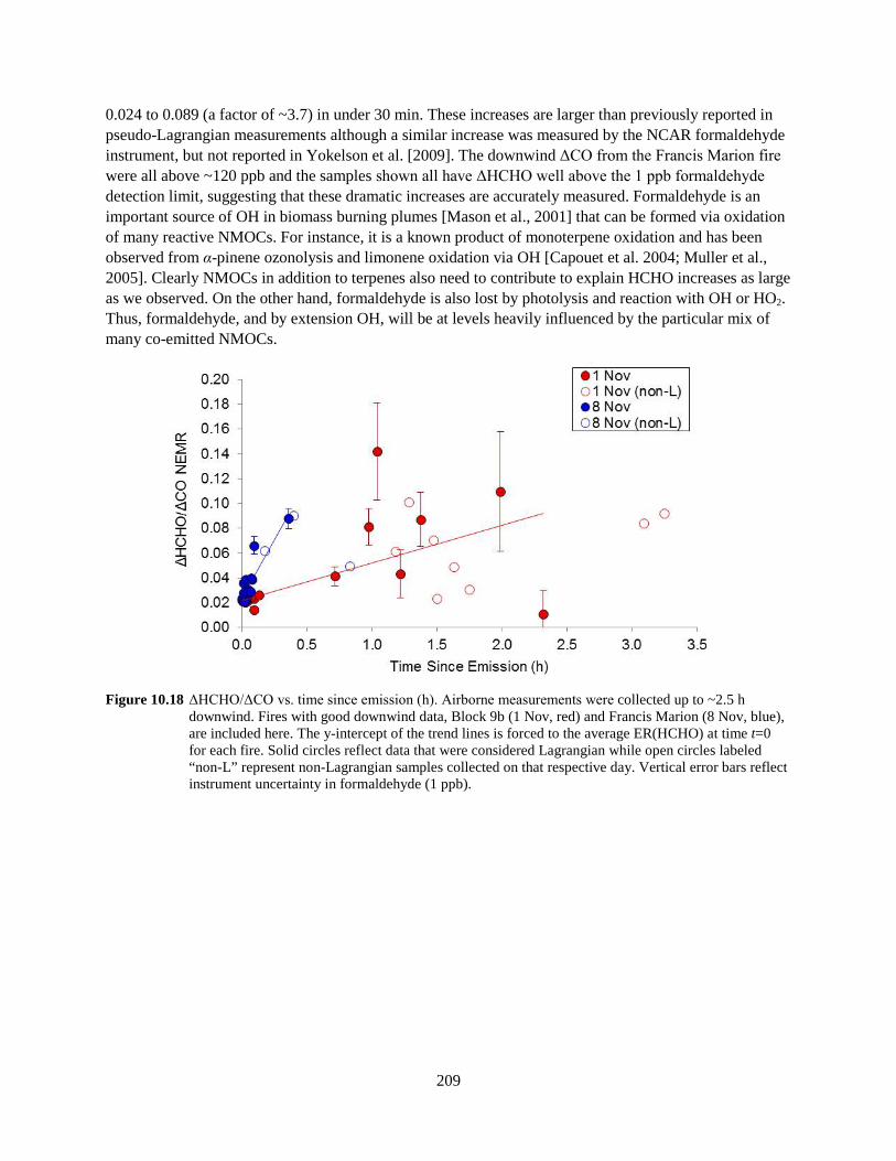
209
0.024 to 0.089 (a factor of ~3.7) in under 30 min. These increases are larger than previously reported in pseudo-Lagrangian measurements although a similar increase was measured by the NCAR formaldehyde instrument, but not reported in Yokelson et al. [2009]. The downwind ΔCO from the Francis Marion fire were all above ~120 ppb and the samples shown all have ΔHCHO well above the 1 ppb formaldehyde detection limit, suggesting that these dramatic increases are accurately measured. Formaldehyde is an important source of OH in biomass burning plumes [Mason et al., 2001] that can be formed via oxidation of many reactive NMOCs. For instance, it is a known product of monoterpene oxidation and has been observed from α-pinene ozonolysis and limonene oxidation via OH [Capouet et al. 2004; Muller et al., 2005]. Clearly NMOCs in addition to terpenes also need to contribute to explain HCHO increases as large as we observed. On the other hand, formaldehyde is also lost by photolysis and reaction with OH or HO2. Thus, formaldehyde, and by extension OH, will be at levels heavily influenced by the particular mix of many co-emitted NMOCs.
Figure 10.18 ΔHCHO/ΔCO vs. time since emission (h). Airborne measurements were collected up to ~2.5 h
downwind. Fires with good downwind data, Block 9b (1 Nov, red) and Francis Marion (8 Nov, blue), are included here. The y-intercept of the trend lines is forced to the average ER(HCHO) at time t=0 for each fire. Solid circles reflect data that were considered Lagrangian while open circles labeled “non-L” represent non-Lagrangian samples collected on that respective day. Vertical error bars reflect instrument uncertainty in formaldehyde (1 ppb).

210
10.16 Open Path Fourier Transform Infrared (OP-FTIR) Studies
10.16.1 OP-FTIR Initial Emissions
Fire-average MCEs and emission factors measured by OP-FTIR for each fire are shown in Table 10.6. The MCEs across all fires showed minimal variability with a fire-average of 0.912 ± 0.004. The fire-averaged MCEs from the LAFTIR (0.842 ± 0.046) and AFTIR (0.929 ± 0.008) indicate larger contributions from smoldering and flaming combustion, respectively. The intermediate OP-FTIR MCE suggests that measured smoke was a mixture of both smoldering emissions and flaming emissions that happened to cross the OP-FTIR path.
Block 6 Block 9b Block 22b Average Std dev MCE
0.917 0.911 0.909 0.912 0.004
Species Formula Carbon Dioxide CO2 1652.8 1642.5 1645.3 1646.9 5.3 Carbon Monoxide CO 94.8 102.1 104.9 100.6 5.2 Methane CH4 2.62 2.70 2.72 2.68 0.05 Ethylene C2H4 1.67 1.58 1.69 1.65 0.06 Ammonia NH3 0.54 0.38 1.22 0.71 0.45 Hydrogen Cyanide HCN 2.11 0.78 - 1.44 0.94 Formaldehyde HCHO 2.31 2.48 2.69 2.49 0.19 Acetic Acid CH3COOH 2.96 3.88 2.76 3.20 0.60 Formic Acid HCOOH 0.40 0.38 0.31 0.36 0.04 Methanol CH3OH 2.09 2.00 1.88 1.99 0.11 Acetylene C2H2 0.81 0.15 - 0.48 0.46 Carbonyls as glyoxala C2H2O2 1.60 2.01 - 1.80 0.29 Furan C4H4O - 0.48 - 0.48 -
Sum NMOC 11.83 12.96 9.34 12.46 0.21 aThe residual spectrum from 2820 to 2850 cm-1 contained features similar to glyoxal, but shifted by several wavenumbers. The feature may have been due to a mixture of oxygenated compounds (most likely carbonyls), but was analyzed using the glyoxal IR cross-section.
Table 10.6 Fire-averaged MCEs and emission factors (g kg-1) measured by OP-FTIR for each of the three pine understory burns at Ft. Jackson.

211
Fire-average EFs are important when assessing overall fire behavior, characteristics of a fire, or when comparing to other fire-average literature EF. That being said, the evolution of the OP-FTIR-measured EF is also useful to inform the comparison to EF measured from other platforms. The drop in the MCE values over the duration of the Ft. Jackson fires suggest that the EF computed for “early” and “late” time blocks (see Figure 10.19) would be mainly indicative of flaming- and smoldering-dominated combustion, respectively. It should be noted that not all fires have a fast transition between high and low MCE [Yokelson et al., 1996] and the division between “early” and “late” can be indistinct. However, this informal separation is useful when considering how burned fuels, sampled emissions, and flaming vs. smoldering combustion can change over the course of the OP-FTIR measurements and how that impacts comparison to other platforms. For the Block 6 fire, “early” was defined from the first OP-FTIR sample (at the fire start 12:38:25 LT) until 13:47:00 LT when a noticeable drop in MCE (or increase in ∆CO/∆CO2, Figure 10.19, shown in dark blue, lower trace) is observed. This signifies changes in the composition of the sampled smoke from mostly flaming combustion to more smoldering combustion.
Figure 10.19 MCE (black) and excess CO (ppm, blue) time series from OP-FTIR on the three Fort Jackson fires. Above the time series, AFTIR (green), LAFTIR (red), and OP-FTIR (blue) sampling time frames are shown to denote the start and end of measurement collection and when the peak intensity signal was observed from a given measurement platform. “Early” and “late” periods of OP-FTIR sampling are denoted in orange and light blue, respectively.

212
10.16.2 FTIR Comparison (OP-FTIR, LAFTIR and AFTIR)
It is of interest to compare the emission factors from all three FTIRs employed during the Fort Jackson burns as each FTIR had a different spatial and temporal perspective on the overall combustion emissions. Figure 10.20 shows a side-by-side comparison of OP-FTIR, LAFTIR, and AFTIR fire-averaged emission factors from the Fort Jackson fires. The fire-averaged MCEs were 0.842 ± 0.046, 0.912 ± 0.004, and 0.929 ± 0.008 for the LAFTIR, OP-FTIR, and AFTIR platforms, respectively. These MCEs make sense given the different mixtures of smoke sampled by each instrument. Additionally, we observe a trend for some smoldering species whose emissions depend more strongly on MCE than fuel type (e.g. CH4, CH3OH, furan) – namely: EF(LAFTIR)>EF(OP-FTIR)>EF(AFTIR), which is consistent with the trend in FTIR fire-averaged MCEs. For other compounds whose emissions are typically more fuel dependent, an EF(OP-FTIR)>EF(LAFTIR)>EF(AFTIR) trend was observed (e.g. CH3COOH, HCHO, NH3), except for EF(C2H2) (a flaming compound) where EF(AFTIR) was greater than EF(LAFTIR). Some of the EF that were higher for OP-FTIR were higher despite an intermediate MCE and they are also known as sticky compounds that are hard to sample in closed-cell systems (NH3 and CH3COOH). Incomplete cell passivation may contribute some of the difference, but losses on cell walls were corrected for in both closed cell FTIR systems and they were not that large when Yokelson et al. (2003) compared AFTIR and OP-FTIR systems under controlled conditions for the same well-mixed smoke samples. Thus, the higher EF for some species may largely be due to sampling emissions from different fuels. The latter idea is supported by the fact that EFs for HCHO, C2H2, and C2H4, which do not suffer from wall losses, are also higher in OP-FTIR than the closed cell systems. In addition the NH3 EF agree well for all the systems on some fires (Block 9b). Fuel differences also likely explain some internal inconsistency in the OP-FTIR results. For instance, on the block 9b fire, the EF for NH3 and CH3OOH are twice as large for the early “flaming dominated” OP-FTIR samples as they are for the later “smoldering dominated samples; despite the fact that these compounds are well-known to be smoldering emissions. The OPAG may be relatively more influenced by recirculated emissions from burning canopy fuels early in the fire. Part of any difference in fuels probed by the two ground-based systems can likely be traced to the sampling procedure of the LAFTIR, which is based on seeking and sampling sources of visible white smoke. Glowing combustion also occurs during RSC and produces high levels of some compounds, but little visible smoke (Figure 3 in Yokelson et al., 1997).

213
Figure 10.20 Side-by-side comparison of fire-averaged emission factors between the LAFTIR (red), OP-FTIR (blue), and AFTIR (green) FTIRs employed during the Fort Jackson campaign.

214
Table 10.7 Emission factors and MCE for select compounds measured during “early” and “late” blocks by OP-
FTIR. Fire-averaged emission factors (g kg-1) from the LAFTIR and AFTIR (Akagi et al., 2013) are also shown.
Emission factors for “early” and “late” smoke measured from the Fort Jackson fires are shown in Table 10.7. CO had the largest EF range, with EF(CO) “late” being almost twice as large as EF(CO) “early”. As mentioned above, we see higher EF for some smoldering compounds like methane and methanol late in the fire associated with lower MCE, but mixed somewhat anomalous results likely rooted in fuel differences for other species such as: ammonia, ethylene, acetic acid, formaldehyde, and formic acid. We also represent data in Table 10.7 as a bar chart (Figure 10.21). Methane and methanol EF appear to follow a decreasing step-wise trend from smoldering-dominant to flaming-dominant platforms,

215
correlating with low to high MCE. Trends are not so straightforward for EF(C2H4) , EF(CH3COOH), or EF(NH3) whose emissions typically depend more on fuels.
Figure 10.21 Emission factors (g kg-1) measured by the OP-FTIR, LAFTIR (red), and AFTIR (green) from the three Fort Jackson fires: (a) Block 6, (b) Block 9b, and (c) Block 22b. The OP-FTIR EF have been broken down into “late” (blue) and “early” (orange).
The extent to which EF correlates with MCE for a given species is best shown by EF vs. MCE plots (Figure 10.11), where a strong negative correlation of EF with increasing MCE is seen for species like CH4 and CH3OH. The EF that appear to deviate from the trend-line are OP-FTIR EF sampled late in the fire’s progression (OP-FTIR “late”), especially for EF(CH4). Nonetheless, we observe reasonable correlation across different instruments and time periods. Burling et al. [2011] report strong correlations (high R2 values) for these same compounds when comparing airborne measurements in temperate conifer forests from U.S. and Mexico, suggesting EF(CH4) and EF(CH3OH) versus MCE relationship is fairly robust across studies in similar fuel types.

216
10.16.3 OP-FTIR Comparisons with the Literature
We can compare the OP-FTIR EF with those from a study that employed a similar open-path FTIR to measure biomass burning emissions from South African savanna fires [Wooster et al., 2011]. The fire-averaged MCEs or ΔCO/ΔCO2 from Wooster et al. (0.913 ± 0.026, 0.095) are similar to those in this work (0.912 ± 0.052, 0.095). This similarity in fire-average MCE or ΔCO/ΔCO2 is surprising considering pine-understory and savanna fuels are intrinsically quite different and have been measured from airborne platforms at different MCE and ΔCO/ΔCO2 (0.931± 0.016 (0.074) and 0.944 ± 0.012 (0.059) respectively, [Akagi et al., 2011; 2013]. Savannas are usually dominated by fine fuels that burn at high combustion efficiency [Akagi et al., 2011] and do not often include large diameter fuels that are highly susceptible to prolonged smoldering. Temperate pine understory ecosystems often have more dead/down debris and below-ground fuels like organic soils that tend to burn by smoldering and/or RSC although that is minimized in prescribed fires. The Wooster et al. [2011] fires were not sampled by an airborne platform, thus, we cannot compare both OP-FTIR and AFTIR MCEs between the studies. Consideration of the MCE observations noted to this point suggests some tentative conclusions: 1) a larger amount of smoldering emissions may be entrained in the lofted plume from pine-understory burns than for savanna fires, reducing the comparative MCE measured from an aircraft, 2) Measured MCEs likely depend on both fuels and the measurement platform, and 3) open-path measurements of fire MCE are likely also sensitive to wind gusts, changes in wind direction, and the duration of the measurements. Thus, fire-averaged MCEs from the OP-FTIR may or may not be the best indicator of fire-average combustion behavior. Additional measurements collected from different platforms are needed to verify these speculations.
Figure 10.22 Comparison of emission factors from this work (blue) and Wooster et al. (2011) (red). EF from this
work have been slightly recalculated using a similar mass balance of carbon as dictated by measured species from Wooster et al. (2011).
We can also compare emissions for several overlapping species other than MCE from this work and Wooster et al. [2011] (Figure 10.22). Emission factors from this work are all within the natural variability of those reported by Wooster et al. [2011], except for NH3. Multiple factors can affect ammonia emissions, the most important being the nitrogen content of the fuel. Measurements in Wooster et al. [2011] were acquired at Kruger National Park where elephant dung is a major fuel component. Dung is known to have a high nitrogen content compared with other main fuel types [Christian et al., 2007; Keene

217
et al. 2006]. While the N content of fuels sampled in this work and in Wooster et al. is unknown, this is one explanation that could justify why EF(NH3) was significantly higher in Wooster et al. [2011].
10.16.4 Estimating Fire-line Exposure to Air Toxics Using the OP-FTIR Results
We think it is likely that the AFTIR measurements may best represent overall fire emissions. However, it is also likely that the OP-FTIR, by virtue of its position on the fire perimeter gives the least biased assessment of smoke exposure affecting personnel deployed on fire containment lines where smoke is flowing over the control line during “black-lining” operations. The LAFTIR samples are also probably relevant to estimating exposure for personnel who actively engage in extinguishing point sources of the type sampled by LAFTIR. Smoke can affect human health via numerous, complex, and poorly understood mechanisms. Firefighters, burn managers, and other wildland fire personnel are subjected to a complex mixture of combustion-generated gases and respirable particles that includes toxic and carcinogenic compounds. Wood smoke contains at least five chemical groups that are classified as known human carcinogens by the International Agency for Research on Cancer (IARC), along with other species classified by the IARC as probable or possible human carcinogens, and at least 26 chemicals listed by the U.S. EPA as hazardous air pollutants [Naeher et al., 2007]. Adverse health effects caused by smoke emitted during a fire can include upper respiratory symptoms [Swiston, 2008], neurological symptoms, and potentially cancer (though previous studies have not yet found a strong link between the two, [Demers et al., 1994]). Only a few studies in the literature have evaluated occupational exposure to smoke among firefighters [Materna et al., 1992; Reinhardt and Ottmar, 1997; Reinhardt and Ottmar, 2004].
In many countries, laws and guidelines have been established to help reduce exposures to potentially harmful levels of toxins and to prevent work-related injury and illness. Average concentrations over time and peak, or maximum exposures, are both of concern. In the U.S., the Occupational Safety and Health Administration (OSHA) set legal exposure limits in the U.S. known as permissible exposure limits (PELs) and short-term exposure limits (STELs) for each of these cases, respectively. A PEL is a time-weighted average (TWA) concentration given an 8-h exposure while a STEL addresses the exposure over a 15-30 minute period of maximum exposure during a given work shift and is designed to control peak exposures of fast-acting toxins. Ceiling limits are also used to regulate exposure to chemicals that may have immediate effects. While OSHA exposure limits are enforceable by law, the National Institute of Occupational Safety and Health (NIOSH) provide exposure guidelines analogous to those from OSHA. NIOSH is part of the Centers for Disease Control and Prevention (CDC) and was established at the same time as OSHA to provide Recommended Exposure Limits, or RELs, as TWA concentrations for an 8-h or 10-h workday. NIOSH also reports STELs as a 15-min maximum exposure. NIOSH limits, being guidelines, are often more conservative than those enforced by OSHA [Sharkey, 1997]. For example, the benzene NIOSH TWA REL (8-h) (0.1 ppm) is 10 times lower than the OSHA TWA PEL (8-h) (1 ppm) and the NIOSH STEL (15-min) (1 ppm) is five times lower than the OSHA STEL (5 ppm) for the same compound. In addition to NIOSH, another set of guidelines is reported by the American Conference of Industrial Hygienists (ACGIH) to assist in the control of health hazards. The ACGIH sets exposure limits known as Threshold Limit Values (TLVs) for chemical substances. The ACGIH TLV is the an 8-h TWA, the TLV STEL is a 15-min maximum exposure, and the ceiling limit, TLV C, is the absolute exposure limit not to be exceeded at any time. For the purposes of this analysis we often report a range when more than one exposure limit is available.

218
Measuring fire-line exposures to various toxins present in smoke in order to compare to e.g. OSHA, NIOSH, or ACGIH exposure limits, is not simple. Fire intensity, fuel composition, and weather conditions are constantly changing and directly affect the fire dynamics and smoke dilution occurring in the work environment (Sharkey, 1997). Different fire types also pose different conditions; several studies have shown that exposures to pollutants were higher among firefighters at prescribed fires than at wildfires [Reinhardt and Ottmar, 2004; Sharkey, 1997]. In addition to fire type, smoke exposure also varies by work activity, e.g. direct attack on prescribed fire ranks high, while activities such as lighting and mop up often result in lower but still significant exposures [Reinhardt and Ottmar, 2004]. Reinhardt and Ottmar (2004) found that CO concentration and smoke exposure were dependent on ambient wind speed for certain job tasks, especially direct attack. For the typical morning prescribed burn, increasing afternoon winds may increase smoke distribution and risk of smoke overexposure for some workers. Various measurement techniques, including electronic dosimeters, liquid chromatography, gas chromatography/flame ionization detection (FID) have been employed to measure different species. This work is the first to assess fire-line exposure using the open-path FTIR technique.
CO (ppm) HCHO (ppm) Average TWA exposures OP-FTIR (burn-average)a,b 6.351 0.147c Reinhardt and Ottmar (2004) (burn-average, 50th percentile)d 6.9 0.075
Reinhardt and Ottmar (2004) (burn-average, 90th percentile)d 23 0.18
Recommended TWA (8-h average) exposure range 25-50e 0.016 - 0.75f
Peak exposures OP-FTIR (max)a,g 32.16 0.825 LAFTIR (max)a,g 641.6 7.665 Reinhardt and Ottmar (2004) (max) >179 1.460 Recommended STEL (15-min) peak exposure range 200h 0.1 - 2.0i aReported as excess mixing ratios. Absolute values will be slightly higher to account for background concentrations. bThe time at the prescribed burns averaged 4:13 h (range ~4-5 h) cSince we do not report HCHO measured from the start to end of the Fort Jackson fires, this value was estimated as ER(HCHO/CO)×OP-FTIR (burn-average) ΔCO. dThe time at the prescribed burns averaged 7 h (range 2-13 h) eLow and high CO values represent ACGIH TWA TLV and OSHA TWA PEL, respectively. fLow and high HCHO values represent NIOSH TWA REL and OSHA TWA PEL, respectively. gPeak exposures represent the average maximum peak exposure from the three different fires measured. hNIOSH ceiling and OSHA STEL (5-min) iLow and high values represent NIOSH STEL and OSHA STEL, respectively.
Table 10.8 Average TWA and peak exposures measured in this work and other studies and recommended TWA and peak exposures.
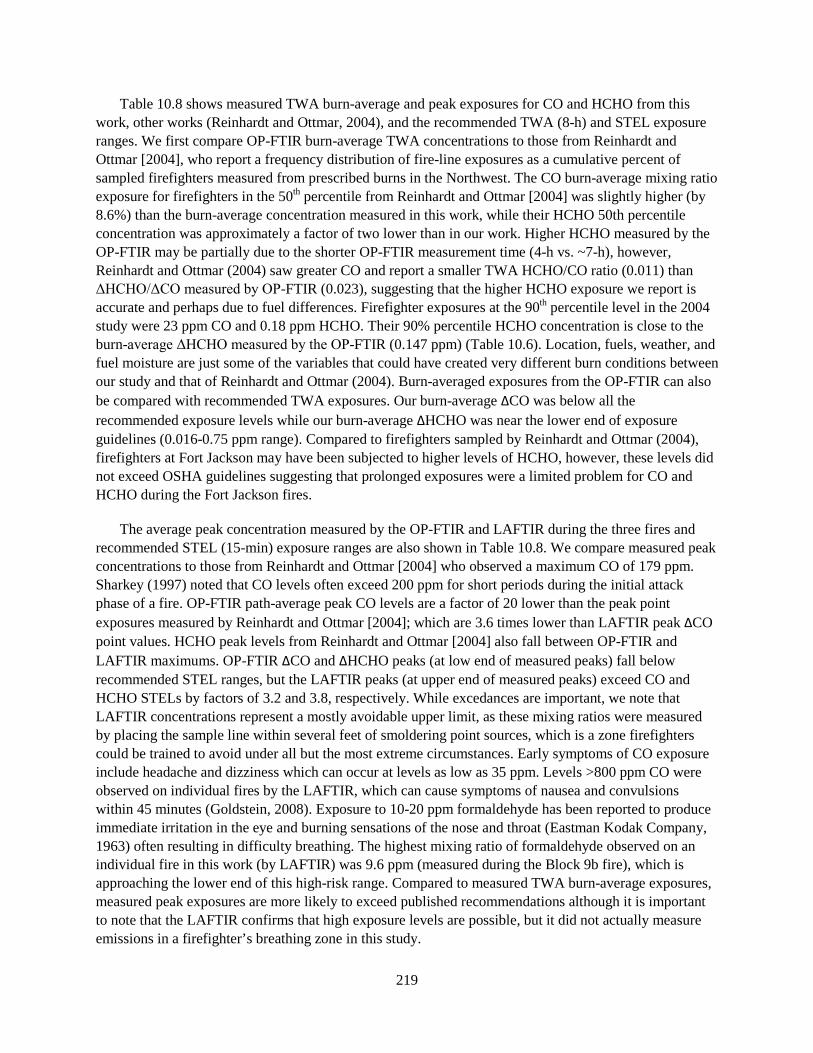
219
Table 10.8 shows measured TWA burn-average and peak exposures for CO and HCHO from this work, other works (Reinhardt and Ottmar, 2004), and the recommended TWA (8-h) and STEL exposure ranges. We first compare OP-FTIR burn-average TWA concentrations to those from Reinhardt and Ottmar [2004], who report a frequency distribution of fire-line exposures as a cumulative percent of sampled firefighters measured from prescribed burns in the Northwest. The CO burn-average mixing ratio exposure for firefighters in the 50th percentile from Reinhardt and Ottmar [2004] was slightly higher (by 8.6%) than the burn-average concentration measured in this work, while their HCHO 50th percentile concentration was approximately a factor of two lower than in our work. Higher HCHO measured by the OP-FTIR may be partially due to the shorter OP-FTIR measurement time (4-h vs. ~7-h), however, Reinhardt and Ottmar (2004) saw greater CO and report a smaller TWA HCHO/CO ratio (0.011) than ΔHCHO/ΔCO measured by OP-FTIR (0.023), suggesting that the higher HCHO exposure we report is accurate and perhaps due to fuel differences. Firefighter exposures at the 90th percentile level in the 2004 study were 23 ppm CO and 0.18 ppm HCHO. Their 90% percentile HCHO concentration is close to the burn-average ΔHCHO measured by the OP-FTIR (0.147 ppm) (Table 10.6). Location, fuels, weather, and fuel moisture are just some of the variables that could have created very different burn conditions between our study and that of Reinhardt and Ottmar (2004). Burn-averaged exposures from the OP-FTIR can also be compared with recommended TWA exposures. Our burn-average ΔCO was below all the recommended exposure levels while our burn-average ΔHCHO was near the lower end of exposure guidelines (0.016-0.75 ppm range). Compared to firefighters sampled by Reinhardt and Ottmar (2004), firefighters at Fort Jackson may have been subjected to higher levels of HCHO, however, these levels did not exceed OSHA guidelines suggesting that prolonged exposures were a limited problem for CO and HCHO during the Fort Jackson fires.
The average peak concentration measured by the OP-FTIR and LAFTIR during the three fires and recommended STEL (15-min) exposure ranges are also shown in Table 10.8. We compare measured peak concentrations to those from Reinhardt and Ottmar [2004] who observed a maximum CO of 179 ppm. Sharkey (1997) noted that CO levels often exceed 200 ppm for short periods during the initial attack phase of a fire. OP-FTIR path-average peak CO levels are a factor of 20 lower than the peak point exposures measured by Reinhardt and Ottmar [2004]; which are 3.6 times lower than LAFTIR peak ΔCO point values. HCHO peak levels from Reinhardt and Ottmar [2004] also fall between OP-FTIR and LAFTIR maximums. OP-FTIR ΔCO and ΔHCHO peaks (at low end of measured peaks) fall below recommended STEL ranges, but the LAFTIR peaks (at upper end of measured peaks) exceed CO and HCHO STELs by factors of 3.2 and 3.8, respectively. While excedances are important, we note that LAFTIR concentrations represent a mostly avoidable upper limit, as these mixing ratios were measured by placing the sample line within several feet of smoldering point sources, which is a zone firefighters could be trained to avoid under all but the most extreme circumstances. Early symptoms of CO exposure include headache and dizziness which can occur at levels as low as 35 ppm. Levels >800 ppm CO were observed on individual fires by the LAFTIR, which can cause symptoms of nausea and convulsions within 45 minutes (Goldstein, 2008). Exposure to 10-20 ppm formaldehyde has been reported to produce immediate irritation in the eye and burning sensations of the nose and throat (Eastman Kodak Company, 1963) often resulting in difficulty breathing. The highest mixing ratio of formaldehyde observed on an individual fire in this work (by LAFTIR) was 9.6 ppm (measured during the Block 9b fire), which is approaching the lower end of this high-risk range. Compared to measured TWA burn-average exposures, measured peak exposures are more likely to exceed published recommendations although it is important to note that the LAFTIR confirms that high exposure levels are possible, but it did not actually measure emissions in a firefighter’s breathing zone in this study.

220
Thus far we have limited our discussion of air toxins to CO and HCHO, though many others exist. Exposure to the other air toxins not measured by the OP-FTIR can, in most cases, be estimated using published normalized excess mixing ratios (ΔX/ΔCO, or NEMR, where “X” is an air toxin whose ratio to CO in smoke was measured in another study) multiplied by the OP-FTIR burn-average CO. Exposure estimates have previously been derived this way by Austin [2008] who used published emission factors and ceiling limits to calculate hazard ratios. We use a slightly different approach: we estimate TWA and peak exposures of high risk compounds using a recent comprehensive set of pine-understory prescribed fire emission ratios from Yokelson et al. [2013] and multiply those ER by the OP-FTIR burn-average and peak ΔCO. For air toxins measured both by OP-FTIR and Yokelson et al. [2013] we can test this approach by comparing calculated versus measured exposures (for HCHO, CH3OH, NH3, Table 10.7). In most cases the calculated EMR were lower than the measured EMR concentrations (by up to 59%), except for HCHO and NH3 measured by the LAFTIR; e.g., the greatest deviation from 1 was the calculated/measured value of 6.60 for the NH3 LAFTIR peak exposure. Given such a high ratio it is likely that this estimation technique is less applicable for some N-containing compounds since their emissions may vary more between studies (Burling et al., 2011). It is also important to note that the emissions data from Yokelson et al. (2013) are for pine understory prescribed fires that burned under different fuel conditions than the fires that the OP-FTIR sampled at Fort Jackson (prescribed fires that were lit after a wet spring versus old growth stands lit after a prolonged drought) [Akagi et al., 2013]. Thus, when emission ratios from other studies are used to estimate smoke exposures there is significant uncertainty. Excluding the high calculated NH3 value mentioned above, the average calculated/measured ratio and 1-σ standard deviation is 0.70 ± 0.37. Despite high variability, this method can be useful approach to estimate exposures for unmeasured compounds of interest.
In this work, measured OP-FTIR TWA fire line mixing ratios and calculated fire line mixing ratios based on OP-FTIR CO did not violate recommended exposure limits for any individual species. Combined exposure limits were also not violated but were more likely to approach recommended limits. Peak mixing ratios measured by the LAFTIR violated STELs for CO and HCHO and calculated peak exposures based on LAFTIR peak CO levels were higher than the STELs for acrolein and HCN. These compounds are some of the more serious irritants and carcinogens that the fire-line may be exposed to. While peak exposures were often observed during initial attack in a study of wildland firefighters [Sharkey, 1997], we show that smoldering combustion measured after the flame front has passed through an area could cause problematic exposures if not carefully avoided. This work agrees with previous works that shift-average TWA exposures may be less of a problem than peak exposures [Sharkey, 1997; Reinhardt and Ottmar, 2004; Austin, 2008], however, combined TWA exposures must be considered for a more realistic assessment of fire-line risk.
10.17 Conclusions – Ft. Jackson Study
The final phase of our study of southeastern U.S. PF emissions succeeded in greatly expanding the range of weather and fuel conditions probed and the scope of smoke chemistry measurements collected. Our previous work measured the PF emissions in intensively managed loblolly pine stands during a wet spring (February-March 2010). The new results reported in this chapter include emissions measurements for relatively undisturbed longleaf pine stands during a dry fall (October-November 2011). The emission factors (EF) measured in 2011 differ by ~13 to 195% from the EF measured in 2010 for numerous organic and N-containing species, even though both phases of the study were conducted in ecosystems that are nominally the same in many simplified global vegetation schemes. Thus, taken together, the 2010

221
and 2011 results now give a much improved picture of the mean and variability in emissions for prescribed fires in southeastern U.S. pine-forest understory fuels. However, much work would be needed to develop an ability to predict the emissions a priori from individual fires of this type with uncertainties significantly smaller than the range in EF we observed.
The expanded suite of measurements produced emission factors for 97 trace gas species from seven PFs— from both airborne and ground-based platforms. The measurements include fire-averaged emission factors for a large suite of terpene compounds emitted by wildland fires for the first time. Limonene and α-pinene were the dominant terpenes emitted. β-Pinene, 4-carene, myrcene, camphene, and isoprene were also measured and the sum of monoterpenes accounted for 0.4-27.9% of initial NMOC mass and equaled ~21% of OA mass. An assessment of likely smoke plume photochemistry indicates that monoterpenes emitted by fires would react mainly with OH during the day and NO3 at night. The known photochemistry of the terpenes and their measured initial abundance suggests that they contributed to our observations of secondary formation of small organic trace gases in the first few hours of post-emission plume aging. For example, we report the first pseudo-Lagrangian measurements of methanol formation in the downwind plumes (an approximate doubling) and also the largest post-emission increases in formaldehyde published to date (an approximate tripling). The observed monoterpenes are known precursors of methanol and formaldehyde, but the large amount of secondary VOCs suggests that other NMOCs, both measured and unmeasured, also acted as precursors. If secondary methanol production in biomass burning plumes is common, then the global methanol source from biomass burning should be scaled upwards. In contrast to the high variability in NMOC emissions, the ΔHCN/ΔCO emission ratio fell within a fairly narrow range that included the ΔHCN/ΔCO ratio for fires in many other ecosystems. This further confirms the value of HCN as a biomass burning indicator/tracer. Our results also support an earlier finding that C3-C4 alkynes may be of use as biomass burning indicators on the time-scale of hours to a day. It was possible to measure the photochemical production of ozone in four of the plumes. Slower O3 production was observed on a cloudy day with low co-emissions of NOx and the fastest O3 production was observed on a sunny day when the plume almost certainly incorporated significant additional NOx by passing over the Columbia, South Carolina metropolitan area. In the mixed BB/FF plume ΔO3/ΔCO reached levels of 10-90% within one hour and total O3 was as high as 104 ppb. With population increasing both in the southeastern U.S. and in developing countries where biomass burning is common, the aggressive ozone increase in mixed emissions could be an increasingly significant public health issue.
We have measured biomass burning trace gas emissions from three prescribed fires at Fort Jackson, South Carolina using an open-path FTIR. The fires were unique in that they occurred on stands that had not burned by prescribed fire in many years and had recently been subject to drought. The OP-FTIR provided a ~30 m, path-integrated sample of smoldering emissions produced upwind and also sampled flaming emissions that were redirected by wind gusts, or right after adjacent ignition and before the local flame front caused significant vertical column development. We compared OP-FTIR-based fire-average emission factors (EF) with fire-average EF measured on the same fires by a roving, land-based FTIR (LAFTIR) and an airborne FTIR (AFTIR) reported by Akagi et al. [2013]. We observe a consistent trend for smoldering species that are not highly fuel dependent (i.e. CH4, CH3OH), where EF(LAFTIR)>EF(OP-FTIR)>EF(AFTIR).We observed a decrease in MCE between the “early” and “late” phases of the OP-FTIR measurements indicative of a shift from flaming-dominated (immediately after adjacent ignition) to smoldering dominated combustion. Emission factors were also calculated separately for these “early” and “late” time blocks to illustrate the temporal change in local combustion and facilitate a more detailed comparison with other EF measurements made on the same fires, but from

222
other platforms. Specifically, Often “early” OP-FTIR EF were most similar to EF(AFTIR) while “late” OP-FTIR EF were most similar to EF(LAFTIR), which is not surprising given the MCE dependence of these species. For other species there was large scatter in the fire-to-fire and species-to-species comparisons, suggesting that the various platforms preferentially sampled the emissions from different fuels. Overall, data from the three FTIR sampling methods employed showed that the method in which the smoke was sampled strongly influenced the relative abundance of the emissions that were observed. We also compare our pine-understory fire EF to EF measured on African savanna fires by a system similar to the OP-FTIR. The EF were very similar between the two studies despite the fact that the fires burned in very different ecosystems, fuel types, weather conditions, etc. This provides further evidence that MCE and trace gas EFs can be highly dependent on measurement platform. The airborne FTIR fire-averaged measurements likely best represented the overall fire emissions in terms of global modeling, but results from the OP-FTIR should be best-suited to estimate fire-line exposures and health risks. Average and peak OP-FTIR mixing ratios and peak LAFTIR mixing ratios were compared to recommended TWA and peak guidelines put forth by OSHA, NIOSH, and ACGIH. We also estimated TWA and peak exposures for many high risk toxins not measured in this work by ratioing NEMR from another more comprehensive study to our real fire line CO data. This is an important approach to estimating exposures since it would be difficult to deploy large amounts of advanced instrumentation on a fire line. TWA individual and combined estimated exposures were not in excedance of recommended guidelines although measured and calculated LAFTIR peak mixing ratios violated STELs for four compounds: CO, HCHO, acrolein, and HCN. Finally, our data support previous findings that peak exposures are more likely to challenge permissible exposure limits than average exposures, suggesting it is important for wildland fire personnel to avoid concentrated smoldering smoke to minimize their risk of overexposure.

223
11.0 Chapter 11
Conclusions and Implications for Implementation/Future Research
11.1 Overview and Summary of Project RC-1649 Results
Project RC-1649, “Advanced Chemical Measurement of Smoke from DoD-prescribed Burns” originated in fiscal year 2008 in order to undertake exactly that objective, namely to use advance instrumental techniques to study in detail the particulate and vapor-phase chemical composition of the smoke that results from using prescribed fire as a land management tool on DoD bases. The measurements and fuels were from several bases throughout the United States, particularly bases in the southeastern U.S. for project RC-1649. More specifically, the SERDP statement of need (SON) originally called for “(1) improving characterization of…fuel consumption” and “(2) improving characterization of air emissions …under both flaming and smoldering conditions with respect to ... volatile organic compounds, heavy metals, and reactive gases.” The work was carried out in collaboration and conjunction with projects RC-1647 and RC-1648.
To briefly summarize our results, the RC-1649 project has delivered state-of-the-art measurements of fuel consumption (FC) on DoD bases and has generated hundreds of the best possible measurements of emission factors (EF) for a very broad suite of trace gases and particulate species. While there were hundreds of measurements of dozens of different vapor-phase and particulate species, we note that the experiments encompassed both laboratory measurements at the U.S. Forest Service Missoula Fire Sciences Laboratory (FSL) (Chapter 6) as well as at two different DoD sites (described in Chapters 7 and 10) as part of RC-1649 as well as at three other sites in collaboration with RC-1647 and RC-1648. The chief deliverable for each effort has been a comprehensive table of emission factors (EF), with the associated tables for the given ecosystem and fire type found in these chapters. A more comprehensive table of EF produced specifically for DoD-relevant ecosystems such as longleaf pine savanna, pine-oak forest, and organic soils has been generated (Ch. 9). The emission ratios (ER) to carbon monoxide (CO) were also measured, and can be used to estimate downwind levels or photochemical changes in the associated species by coupling with data from either municipal or handheld CO monitors. Multiple measurements of chemical transformations in plumes have also been made, largely via airborne sampling.
This report and the associated publications represent thousands of EF results from the different types of fires on various ecosystems, as well as different types of measurements using different types of instruments. To try to oversimplify these many results would be dangerous, and the reader is recommended to study the many results either in turn, or specific to those cases or fuel types that are of immediate interest. Nevertheless, some general observations and conclusions can be drawn from the many studies represented here: The list of species measured in this project is the most extensive smoke characterization achieved to date. This large body of data has been presented in an extensive table of emission factors (EF, Table 8.2, and also in Yokelson et al., [2013]). Table 8.2 breaks out the vegetation types in four main categories: semiarid shrublands, pine forest understory, coniferous canopy fuels, and organic soils. The amount of sampling upon which the data are based was extensive, including both our laboratory and field experiments through 2010 for the first two vegetation types. For the latter two vegetation types (coniferous canopy and organic soils) the EF are based solely on simulated fires in the Missoula combustion facility. Field sampling of those fire types (coniferous canopy and smoldering

224
soils) is thus a likely priority for future work since those fuels are also important on DoD managed wetlands and in wildfires. The EF for less frequently burned stands are also among the most comprehensive fire data ever published (Chapter 10, also Akagi et al., [2013]). The EF from Yokelson et al. [2013] (also Chapter 8), and Akagi et al. (Chapter 10) have been coupled in a freely available EF database on the web maintained by the National Center for Atmospheric Research (NCAR), and represent a truly major effort by multiple scientists supported by several agencies. We note that these studies also provided the most rigorous estimate to date of the abundance of emissions that could not be identified with the technology available when the RC-1649 project started in 2009.
Plume evolution achievements included the first measurement of how fast black carbon (BC) emitted by fires develops a coating [Chapter 10, Akagi et al., 2012]. The biomass burning BC was mostly coated within one hour as opposed to the several days typically required for the process whereby BC is emitted by diesel engines. This is extremely important in terms of climate change, because the coatings increase the absorption of solar radiation by a lensing effect, but they also increase the BC solubility. Increased solubility means the BC has a greater ability to reduce cloud droplet sizes, which causes atmospheric cooling. The coating also greatly increases the rate of removal in the atmosphere, which reduces the lifetime that the BC can warm the atmosphere and the chances of transport to sensitive snow/ice covered regions such as the Arctic [Akagi et al., 2012].
Another key plume aging result discussed in Chapter 10 and in Akagi et al., [2012] was the finding that the PM/CO ratio decreased with initial plume aging due most likely to evaporation of organic gases from the smoke aerosol. This is in stark contrast to fossil fuel emission where a huge increase (factor of five to ten) increase in PM/CO is seen after emission due to secondary aerosol formation (SOA). In an earlier study [Yokelson et al., 2009] we had observed SOA-driven increases in PM/CO in a Mexican biomass burning plume. We hypothesize that the different outcomes are due to the different post emission environments and this could have smoke management implications. However, the EF database, particularly for aged plumes, is not large yet and understanding SOA in BB plumes remains a priority for future research. Some of this research was accomplished in the South Carolina campaign, but the analysis and publication has been delayed due to a team member departing the research program to take a faculty position in Korea. Nevertheless, we note that two important plume aging results from the 2011 South Carolina study (Chapter 10) are already published in the open literature: 1) We observed faster secondary ozone formation in smoke plumes that mixed with urban emissions [Akagi et al., 2013]. This has obvious smoke management implications. We also observed 2) the generation of terpene oxidation products in downwind plumes for the first time. This is of importance to validate smoke models and may not have immediate smoke management implications. Fast formation of large amounts of gas-phase organic acids was also observed post emission by Akagi et al. [2012]. This is important mainly as a demonstration that the plume evolution is strongly influenced by the currently unidentified species. The chemistry of the known precursor species cannot account for the observation in models and thus this finding provides evidence of the importance of continuing to target improved speciation of the initial emissions.
To recapitulate, the statement of need originally called for “(1) improving characterization of…fuel consumption” and “(2) improving characterization of air emissions …under both flaming and smoldering conditions with respect to ... volatile organic compounds… and reactive gases.” As discussed, we have made the most progress on measuring initial emissions and ozone formation, measuring dozens of gases as has been detailed in Chapters 6, 7 and 10, but with the most remaining work to be done in the area of SOA. In particular, the most relevant progress is perhaps in the area of black carbon. We made the first measurements of initial BC and BC coating rates with modern non-filter-based techniques for domestic

225
fires in US. Largely as part of the SERDP-funded studies, but also in conjunction with the JFSP-funded projects, we have a research paper in progress that compares the new method (single particle soot photometer (SP2)) with older filter-based elemental carbon (EC) determinations.
11.2 Advancement of Enabling Technologies and Fundamental Science via RC-1649
In addition to the many accomplishments that directly address the SON, namely the determination of a multitude of emission factors that are summarized in 11.4 and 11.5, the project has also effected many accomplishments in terms of both enabling new technologies and also advancing fundamental science. Most of the enabling capabilities work has been in the field of Fourier Transform Infrared spectroscopy (FTIR). The RC-1649 project has made great advances in the hardware, chemometric software and supporting reference data aspects of this important branch of physical and atmospheric chemistry. Infrared spectroscopy is one of very few methods for remote sampling of gases; it offers both high precision and good sensitivity without sampling artifacts. The FTIR and optics systems that were developed and implemented have been detailed in Chapter 3. For both the FSL laboratory measurements as well as the field experiments, a factor of nearly 20x improvement in sensitivity has been recognized as documented in Figure 3.5. This marked increase in signal-to-noise ratio has translated directly into more species being detected with greater accuracy and greater sensitivity. The increased sensitivity and selectivity has been further augmented by improvements to the MALT software (Chapter 4) that allowed faster determination of gas-phase mixing ratios, also with improved sensitivity. These combined improvements have together allowed additional species to be detected and allowed for more reliable determinations of emission factors, both in terms of sensitivity and precision.
Another area where we have seen large accomplishment for enabling technologies is in expansion of the infrared spectral database. The project has recorded the quantitative IR spectra of more than 60 new chemical species (cf. Chapter 5). These new spectra have enabled several collaborative studies in basic physical science, as evidenced by the papers by Profeta [2011], Johnson et al. [2013], or Williams et al. [2013]. More importantly, the new quantitative spectra allow analyte detection via either broadband FTIR methods [Johnson et al., 2010] or via more sensitive infrared laser spectroscopy methods such as those using quantum cascade IR lasers, e.g. Taubman et al. [2004]. In terms of this project the availability of the newly generated reference data has translated directly into the detection and quantification of several new species that heretofore had not been observed with IR spectroscopy in biomass burning. We have compiled a database of quantitative infrared spectra that determine for each gaseous species the absorption cross section ε as a function of wavelength. These data are being used to help determine the concentrations (C) of many different species by using the Beer-Lambert Law (absorption, A = εCl, where l is the optical path length) to determine the spatially and temporally resolved concentrations C of various molecules. While IR spectroscopy can readily derive the gas-phase concentrations, quantitative reference data are necessary. As detailed in Chapters 6 to 10, some of the newly observed species include classes such as terpenes, hemi-terpenes and the associated oxygenated volatile organic compounds (OVOCs) and oxidation products. Specific examples include lab and field measurements of species such as glyoxal (C2H2O2), Glycolaldehyde (C2H4O2), nitrous acid HONO, isocyanic acid (HNCO), α-pinene, β-pinene, D-limonene, phenol as well as others. An example of such newly derived observations is seen below in Figure 11.1 for the case of isocyanic acid which is taken from the paper by Roberts et al. [2010]. This release of HNCO during PF burning and its potential health effects led to subsequent publication in the Proc. National Academy of Sciences [2011].

226
Figure 11.1 Two consecutive infrared spectra of HNCO source output (red, blue) and PNNL reference spectrum
(black) as used to quantify the mixing ratio of isocyanic acid during the 2009 Fire Sciences Lab burns.
The detection of these several new species using infrared spectroscopy has lent credence to the technique as one of the few methods for portable, sensitive and specific method for remote detection of vapor-phase biomass burning effluents. In many of these cases, the detection of the new species (e.g. Figure 11.1) can be directly attributed to the availability of the reference spectra in the library. Just as a fingerprinting method is only as valuable as the entries in the fingerprint database, the detection capabilities of the IR method are only as effective as the number of entries in its library; further expansion of the infrared library as well as infrared field methods, particularly those using laser spectroscopy, are thus suggested as future courses of research.
11.3 Effects of Prescribed Fire Effluents on Climate Change The global warming potential (GWP) of greenhouse gases, namely their ability to warm the earth’s atmosphere, is directly proportional to two key factors: 1) their concentration or mixing ratio in the atmosphere - which can have certain temporal and spatial variabilities - as well as 2) their ability to absorb infrared radiation, especially between 5 and 200 µm (2,000 to 50 cm-1) the wavelengths where the earth is known to act as a “pseudo - blackbody” emitter. Of particular importance is the 7 to 13 µm longwave infrared (LWIR) window [Forster et al., 2007]. Any radiation emitted by the earth that is not re-radiated all the way into deep space is absorbed by atmospheric gases or aerosols and warms the earth’s atmosphere. Any gas that contributes to this phenomenon is by definition a greenhouse gas.
It has recently been recognized that, while counterintuitive, reducing pollution may in some cases actually contribute to global warming [e.g. Arneth et al., 2009]. The present research project on the emissions from DoD prescribed fires directly addresses these issues and trade-offs: The main greenhouse gases in the Earth's atmosphere are water vapor, carbon dioxide, methane, nitrous oxide, and ozone [Forster et al., 2007]. The first three are directly emitted by fires, whereas ozone is formed

227
photochemically in smoke plumes [Yokelson et al., 2009]. Fires are the second largest source of CO2 globally (after fossil fuel combustion), but biomass burning within the US is not a major national CO2 source [Forster et al., 2007]. Methane, the third most important greenhouse gas is emitted by fires at about 1% of CO2, but has stronger infrared absorption coefficients. [Yokelson et al. 2008)]. However, methane’s comparative importance to CO2 is higher due to its global warming potential (GWP, as discussed in Forster et al., 2007). The GWP mentioned above is a quantitative measure of how much a molecule contributes to warming relative to a molecule of CO2. The GWP depends on the following factors, each of which is quantified: (1) the strength of absorption of infrared radiation by a given species, (2) the spectral location of its absorbing wavelengths, and (3) the atmospheric lifetime of the species. Because the GWP depends on the atmospheric lifetime it also depends on the time horizon for which it is calculated. The accepted standard set by the UN is 100 years. Since CH4 has a 100 year GWP of 12, its contribution to warming is then about 12% of that of CO2 even though its emissions are only 1% as large.
As mentioned, biomass burning is a known major source of both particles and atmospheric trace gases, including the five species just discussed and thus affects climate. Contributions from in situ or remote sensing measurements acquired from laboratory-, ground-, air-, or space-based platforms and modeling at many scales are all critical to assess the climate effects of PF, as is the proper coupling of these studies. As discussed in the previous section, advances in infrared spectroscopy in RC-1649 have greatly increased the ability to detect to several species on multiple platforms. The advances made, however, not only increase the ability to detect certain BB gases in terms of general EF, but also provide two distinct methods that help determine a gas’s global warming potential (GWP), and thus its effect on climate. The first arises because in order to know the global warming impact of any gas, it is necessary to quantify how much of it is in the atmosphere. The methods described here, in particular the improved infrared detection as along with the freely distributed reference data, benefits not only to the RC-1649 project, but many atmospheric research efforts. The IR spectra that have been derived by the project can be used in a multitude of ways, but the most important of these is that the data can be used to quantify concentrations of molecules from both in situ measurements as well as from airplanes, satellites, etc. In particular, using several methods, but especially infrared spectroscopy, we have reported the EF of hundreds of species, and the IR database can be still further used to quantify concentrations of dozens more new potential GHG species whose atmospheric burdens are heretofore still unknown.
During the course of the RC-1649 project we measured the EF in 77 lab fires and approximately 25 field fires for both CO2 and CH4 and we also obtained a rare measurement of the rate of ozone formation in one smoke plume (Chapter 6, 7 and 10). As a concrete example we have also measured many other trace gas emissions during the project in both the lab and field that affect climate. We also measured CO EF for 77 lab and ~25 field fires CO is emitted at about 10% of CO2, but has a low GWP because it has no absorptions in the 7-13 micron window and because its atmospheric lifetime is only 1-6 months. However, CO is the main sink for OH, which also determines the CH4 lifetime. Thus more CO in the atmosphere will increase the CH4 lifetime and consequently the CH4 GWP.
Importantly, we have also measured EF for dozens of non-methane organic compounds (NMOC. The individual NMOC are typically emitted at less than 10-50% of CH4. The NMOC also have much shorter lifetimes than CH4 (e.g. hours to weeks instead of years as for CH4) and thus lower GWPs. An example is propane which has a GWP of 3. However, the sum of all NMOC emitted will be larger than the CH4 emissions and so the direct effect on climate of NMOC is not negligible. Further, the NMOC GWP are larger if calculated on a shorter horizon and thus controlling the emissions of short lived species such as NMOC (or black carbon) may provide a rapid climate benefit [Unger et al., 2010]. The NMOC also affect

228
climate through three indirect effects (1) they consume OH, (2) they contribute to ozone formation, and (3) they can contribute to secondary formation of aerosol, which has climate effects described in part 4. Globally, fires are the second largest source of NMOC after vegetation [Yokelson et al., 2008]. We also measured EF for NOx for all 91 fires studies in this project. NOx has several indirect climate effects of which the most important is its role as the sole precursor to tropospheric ozone [Forster et al., 2007]. Thus, while the chemistry is complicated and interwoven, the SERDP funded 1649 studies have greatly helped characterize the emission of many trace gases that are key players, both as greenhouse gases themselves, as well as affecting the concentrations of other greenhouse gases.
The second manner in which the project has contributed to better understanding climate change science is that the PNNL IR data can be used to compute the quantitative infrared extinction coefficients that determine the relative ability of gases to contribute to the greenhouse effect; i.e. new global warming potentials can be calculated for many species for first time. As discussed above in points (1) and (2), in order to know how much of the Earth’s infrared radiation is absorbed (A) in the Earth’s atmosphere, one needs to know the concentration of that species (C) (by whatever analytical method) and its infrared extinction coefficient ε as related by Beer’s law A(λ) = ε(λ)Cl. Regardless of whether the gas concentration C is quantified by IR spectroscopy, mass spectrometry or any other technique, the efficacy of a gas at absorbing infrared radiation at certain wavelengths is a key factor in determining its global warming potential. The quantitative PNNL database spectra provide the extinction coefficients ε(λ) as function of wavelength λ that are used by the atmospheric modelers to determine the global warming potential. While at first blush it would seem there are many available reference spectra, in fact there is a real dearth of quantitative values. [Commercial suppliers have hundreds of thousands of such spectra, but most have an “arbitrary” y-axis.] There are but a few other sources of quantitative infrared data such as the HITRAN molecular database, which typically have very high spectral resolution but quantitative cross sections for only a limited number of species; e.g. the HITRAN database has data for just 42 different molecules. These include mostly smaller molecules such as CO, CO2, NH3 and so on, but essentially none of the volatile organic compounds (VOCs) or oxygenated-VOCs (OVOCs) that have recently been demonstrated to be key effluents of biomass burning phenomena, such at the 60+ molecules associate with PF recently added to the PNNL database.
Figure 11.2 Plot from PNNL database showing the effects of strong IR cross sections ε(λ) values. While CO2 is a powerful GHG due to its high concentration, species such as butadiene could also be powerful climate forcers due to stronger cross-sections. In this plot butadiene is seen to have IR absorption coefficients more than 100x stronger than CO2 (species plotted with 1 ppm concentrations in left frame).

229
An example of how the infrared cross sections are understood in relation to their GWP can be seen in Figure 11.2. Some gases such as CF4 or 1,3-butadiene may have relatively low atmospheric concentrations, but have enormous IR cross sections in key “spectral windows” which can increase their global warming potentials. In the longwave infrared plot shown above, the butadiene is seen to have infrared absorption coefficients more than 100x stronger than CO2 (both species plotted with 1 ppm concentrations in left frame). The new IR cross section data allows us to answer these questions for the first time. While other factors also must be accounted for including atmospheric lifetime, because of this SERDP project and the original PNNL database, the total number of spectra that are now available to use in GWP calculations is now nearly 600 different species. These infrared cross-section data are publicly available at nwir.pnl.gov. Such data offer the only means by which one calculate the global warming potential of a particle or gaseous species: it is recommended to continue to expand such studies to better understand climate change.
11.4 Synopsis of Lab- versus Field-Measurements and Data Fusion
It is clear that ultimately one would want to be able to measure as many field fires as possible in order to obtain the most realistic emission factors as possible, not only for different chemical species but for different ecosystems, fuel types, fuel conditions etc., as well as to better distinguish ground-based versus airborne emissions. Due to the enormous expense and logistical challenges of field work, this is obviously not possible. The alternative is to thus conduct many laboratory fires, and compare and couple the emission factors derived in the laboratory so as to be able to correlate them to those of field EF. The greatest advantage of lab studies over field work is that one can readily deploy more instrumentation on the lab fires allowed many more important species to be measured than was possible on the field fires. Such additional species, including the unidentified ones, could significantly influence the post-emission smoke plume chemistry if they were present in similar amounts in the smoke from field fires [Trentmann et al., 2005; Alvarado and Prinn, 2009]. It is thus important to explore how well the EFs measured on laboratory fires as described in Chapter 6 can represent the EFs for field fires.
As described in chs. 6-8, many key trace gases have been measured using a nearly identical FTIR-based approach on both the lab and field fires, as was PM2.5. By removing the uncertainty that arises for measurements made with different types of instruments, using the same technique allows us to make a fairly direct comparison of the lab and field data for a suite of many species that includes both organic and inorganic gases, as well as compounds associated with both flaming and smoldering phases. We have made comparisons knowing that the fire emission factors depend on the modified combustion efficiency, a proxy for the relative amount of flaming v. smoldering combustion. As shown in Chapter 8 and re-plotted as Figure 11.3 we have the lab and field EF versus MCE for key species measured in both the laboratory and field. Each plot compared all the EF from all the lab and field fires together on the same graph for one of the two major ecosystem types (pine-understory and semiarid shrublands). The lab EFs were computed via the carbon mass balance method using just the FTIR species for this comparison to avoid a small downward bias on the lab EF. Typical examples are found in Chapter 8 and in Figure 11.3.

230
Figure 11.3 Comparison of EF versus MCE from the laboratory and the field fires for smoldering compounds and PM2.5 for pine understory (left column) and semiarid shrubland (right column). The “Grd” (green symbols) indicate data for residual smoldering combustion provided for context. The emission factors vs. MCE are for the species methane, methanol, formaldehyde and PM2.5, respectively, top to bottom.
In this example, we focus first on the lab/field comparison for methane and gas-phase NMOC produced primarily by smoldering combustion (e.g. CH3OH and HCHO) in the top three rows of Figure 11.3. For all three of these species (and others not shown) there is clearly good agreement between the lab and field for the pine-understory fuels (left column), but a large offset to lower EF in the lab for the semiarid shrubland fuels (right column). We speculate that the offset to lower EF for smoldering compounds from the lab semiarid shrubland fires could have partly resulted from lower fuel moisture in the lab fuels as discussed in Chapter 8. PM2.5 emissions also tend to increase with lower MCE similar to the smoldering NMOC as shown in the bottom row of Figure 11.3. However, in the case of PM2.5, the EF for pine-understory fuels are offset to significantly lower values for the lab fires and the EFPM2.5 for semiarid shrubland fuels agree fairly well at lower MCEs when measured in the lab or field.
The plots for the pine-understory fuels in Figure 11.3 also show the RSC EF measured from the ground (chapter 7) for context and because of the potential high contribution of RSC to air quality

231
impacts and wildfire emissions that we noted earlier. The RSC measurements are of individual smoldering fuel elements rather than a blended convection column and thus do not normally fit the pattern established by airborne measurements (discussed in chapter 10). In Table 8.1 we showed the results of treating our current lab and field EF with both approaches previously used to “transform” lab EF to field EF. Specifically, columns 5, 6, 11, and 12 showed the predictions of the lab MCE-based equation adjacent to how those predictions compare to the field data for the pine and semi-arid ecosystems, respectively. Columns 7 and 13 show the lab/field EF ratios for the two ecosystems. The inverse of the average ratio for each ecosystem is the simple correction factor in the approach employed by Yokelson et al., [2008]. As discussed in Chapter 8, the lab-average EFs are, on average, 110 ± 60 % of the field-average EFs suggesting that a relatively un-biased estimate of the field average EF can be obtained simply and directly from the lab-average EF with about 50% uncertainty on average. Although the equation-based approach appears to work “perfectly” on average, no statistically significant increase in accuracy results from applying the more complex equation-based mapping approach to the pine-understory data. As a result we suggest that the lab-average EF presented for ~330 additional smoldering species for pine understory fuels can be used directly to estimate the EF for these species from field fires in pine-understory fuels.
For semiarid shrubland fuels, the lab-based equations predict field EFs a bit closer to the EFs measured on the field fires than simply using the lab average EFs. However, both approaches require subsequently applying a large normalization factor to get good agreement and have essentially equal error of prediction. Thus, applying an equation and then a normalization factor, rather than just applying a normalization factor to the lab average EFs for over 300 compounds does not add enough accuracy to justify the added complexity. As a result, we suggest that dividing the lab EFs for smoldering compounds by 0.37 (see the bottom of column 13) or, equivalently, multiplying by 2.7 is the preferred way to predict the EFs expected in the field for semiarid shrubland fires. The normalization factor is large, but we note that applying this factor makes the EF for the lab semiarid shrubland fires closer to the EF for the lab pine-understory fires, which recovers the small EF dependence on ecosystem that was observed in the field.
An obvious difference between field and laboratory fires is the ubiquitous presence of wind in the field to assist fire propagation. Spread rates measured in the field are typically 0.2-1.6 m s-1 for grass fires (Shea et al., 1996; Stocks et al., 1996), 0.06-0.23 m s-1 for chamise and mixed chaparral fires [Chandler 1963], and 0.01-0.05 m s-1 for prescribed understory fires (Yokelson et al., 1999). On a one meter fuel bed in the lab, spread rates this high would lead to fires that last only ~0.6-100 s. In the lab fires reported here we initially oriented the fuels in a natural vertical position at loadings consistent with literature values, but only the pine understory fuels burned well in this arrangement. To get greater than approximately ten percent fuel consumption for the semiarid shrubland fuels in the lab (in the absence of wind) it was necessary to stack them horizontally. The fuel moisture was also different between the laboratory and field. Live fuel moistures were 40-70% for semiarid shrubland fuels in the field and the lab fuels burned at 18 ± 15% and 14 ± 9.1% for the pine understory and semiarid shrubland fuels, respectively. The overall fuel consumption in the lab (field) was 15 ± 10 (7.0 ± 2.3) Mg ha-1 and 23 ± 10 (7.7 ± 3.7) Mg ha-1 for pine-understory and semiarid shrubland, respectively. Thus, our pine-understory lab fires had a total fuel consumption that was closer to what we observed in the field, but the fuel consumption on our lab semiarid shrubland fires was still close to the literature average for field fires. Another difference between field and lab fires is that the emissions measured on the sampling platform in the lab were sometimes briefly at temperatures as high as 330 K, whereas the coolest plume samples in the field were

232
as low as 280K. Huffman et al., (2009) found that about 20-25% of biomass burning organic aerosol could be volatilized by a sustained 50°C increase in a thermodenuder. However, aerosol, as noted above, is predominantly a smoldering species and most of the aerosol in the lab fires was measured when the smoke plume was near room temperature. Thus it is unlikely that temperature differences caused significant lab/field differences. After a detailed consideration of the relevant data we conclude that the fuel moisture differences between the lab and field may contribute the most to observed differences, but that the lab data, after normalization for the semiarid shrubland fuels, provide a useful representation of the somewhat variable emissions from field fires.
As was detailed in Chapter 8 we have presented a retrospective analysis of a series of studies that included measurements of biomass burning trace gas emissions with the most comprehensive selection of instrumentation to date as well as measurements of fine particle emissions, selected particle species (including elemental carbon), and biomass fuel consumption per unit area on prescribed fires. We have confirmed that studying laboratory biomass fires can significantly increase our understanding of wildland fires, especially when laboratory and field results are carefully combined and compared. The analysis presented here provides a set of emission factors (Table 8.2) for modeling prescribed fire smoke photochemistry and air quality impacts that is greatly expanded beyond what was previously available. The new set of emission factors includes data for hazardous air pollutants (Table 8.4) and numerous precursors for the formation of ozone and secondary aerosol. New measurements of the mass of fuel consumed per unit area are presented in Table 8.5 that should be useful for model predictions of the amount of smoke produced by prescribed burns. Profiles of the elemental composition of prescribed fire particulate matter are presented that can be used to estimate prescribed fire contribution to ambient PM2.5 (Reff et al., 2009). The results of this series of studies can be applied most confidently to understanding springtime pine-understory prescribed fires in the southeastern US and to a lesser extent to prescribed fires in semiarid shrublands of the southwestern US.
11.5 Relevance of findings to land managers
This section summarizes the relevance of our findings to land managers, particularly in the context of managers that must use PF as a tool while still meeting air quality standards and safety and/or health and environmental considerations. It thus comprises a set of non-binding recommendations for guidance and tools that relate to the use of emission factors derived as a course of these studies as related to human health as well environmental effects. Due in part to the research reported here, it now seems unlikely that smoke managers will have to allow for high amounts of SOA when forecasting downwind impacts of their burns (Chapter 10, also Akagi et al., [2012]). It also seems likely that ozone production could be minimized by avoiding smoke plume interaction with sources of NO2 such as urban areas (especially on weekdays, e.g. due to automobile traffic) or active power plants as discussed in Chapter 10.6 and 10.15, as well as [Akagi et al., 2013]. It will also be possible to develop more accurate smoke chemistry models using the better initial emissions data we have provided. The process of model improvement is already underway on several fronts. One of the key deliverables of the project was a set of emission factors for prescribed fires in temperate ecosystems that could be used by base managers. In Table 8.2 we presented our best estimate of the emission factors for PM2.5 and all the trace gas species measured in this series of studies (including unidentified species) for prescribed fires in pine forest understory and semiarid shrubland and fires in coniferous canopy fuels and organic soils. The EFs in Table 8.2 were generated by applying simple selection rules to the lab emissions data and the field emissions data in Table 8.1. In Table 8.2 we

233
selected the average emission factor for a species that was measured on the field fires during the four field deployments for all the species that were measured in the field. We used the average lab fire EFs when no field measurements were made of that species. For the semiarid shrubland fires, the lab EFs for smoldering compounds were multiplied by 2.7 to better represent field fire emissions as discussed above. In practice, this affected all the lab data used from the semiarid shrubland category except alkynes higher than C2H2 (detailed in chapter 10) and SO2, HCl, and HNCO, which were not measured in the field and were identified as flaming species in the lab study by their temporal correlation with CO2 [Burling et al., 2010; Roberts et al., 2010].
Secondary inorganic aerosol (SIA) could be formed primarily from nitrogen containing gases (NH3 to ammonium and NOx to nitrate) and SO2 (to sulfate). The emissions of these precursor gases are heavily dependent on fuel chemistry with foliage and crop residue having elevated levels. In this study the emission factors of the NH3, NOx, and SO2 sum to about 4 g kg-1 compared to a generic EFPM2.5 of ~10 g kg-1, suggesting that SIA should not be neglected in smoke plume models. Substantial SIA has been measured in the field in biomass burning plumes [Alvarado et al., 2010; Akagi et al., 2012a].
The prospects for fully mechanistic modeling of smoke plumes and the adequacy of using only known, measured species can be assessed from Table 8.3 as well. For the two main fuel types ~31% of the non-methane organic carbon (NMOC) mass is unidentified and ~72% of the mass of NMOC is unidentified for the one lab fire in smoldering Alaskan organic soil. In addition, the majority of unidentified NMOC are in our “IVOC+SVOC” category suggesting the need to model SOA with semi-empirical approaches for some time to come [Robinson et al., 2007]. Two important examples of how this data set could improve modeling of global biomass burning are described next. (1) Peat combustion is a major global type of biomass combustion especially in El-Niño years [Page et al., 2002; Akagi et al., 2011]. We note that our laboratory smoldering organic soil fire had the largest PM2.5 emissions (20.6 g kg-1), the largest emission factor for NMOC, EFNMOC (179 g kg-1), the largest ratio of NMOC to PM2.5 (~8.7), and the largest fraction of NMOC in our “IVOC+SVOC” category (0.64). This fuel type may have very high potential for SOA, but it is also the least well characterized. Table 8.2 and Table 8.3 provide important new emissions data for smoldering organic soils, but also highlight the need for further study of this source. (2) Akagi et al. [2011] estimated global NMOC emissions from biomass burning using only previously available information. Their estimate of total EFNMOC (including unmeasured species) for temperate forests of 23.7 g kg-1 (their Table S4) is close to the total EFNMOC measured in this work for the pine-forest understory fires (~27.6 g kg-1). Akagi et al. (2011) derived an estimate of total EFNMOC of 97.3 g kg-1 for peatland fires, which is actually well below the value of 179 g kg-1 measured for smoldering organic soils in this work. The global NMOC estimate of Akagi et al. [2011] was 4-7 times larger than some previous estimates of organic trace gas emissions from fires that ignored oxygenated organic compounds and unidentified species, but it is strongly supported by this work suggesting that global model runs with much larger NMOC emissions per unit mass of biomass burned are needed.
As shown in our work, the lifetime of BC emitted by fires is likely much shorter than the lifetime of BC emitted by industrial sources. When one also factors in other recent findings there is very little reason to suspect that reducing prescribed fire in the US will be of any value in preserving snow and ice in the Arctic. Only surface level BC hastens snow melt and the BC at upper levels actually helps cool the surface and shield the snow and ice. Our HYSPLIT trajectories showed that much of the BC from US prescribed fire emissions is removed by precipitation and what does make it to the Arctic is primarily at high altitudes. Recent work by Stohl et al. [2013] shows that oil and gas flaring actually accounts for 42% of surface level BC in Arctic and that much of the rest is from seasonally adjusted wood burning for home
234
heating in Europe. http://www.atmos-chem-phys-discuss.net/13/9567/2013/acpd-13-9567-2013.html. Similarly, BC on snow in Finland was also likely underestimated due to ignoring residential wood-burning: http://www.atmos-chem-phys.net/13/4033/2013/acp-13-4033-2013.html. When one also factors in the long-time, widespread knowledge that fire aerosol has a net cooling effect because OC/BC in biomass fire emissions is >>1 it becomes clear that the impact of US prescribed fires on the Arctic is likely minimal.
In terms of best representing the conditions to which a firefighter or person on the fireline is exposed, we think it is likely that the AFTIR measurements as discussed in Chapter 10 may best represent overall fire emissions. However, it is also likely that the OP-FTIR, by virtue of its position on the fire perimeter gives the least biased assessment of smoke exposure affecting personnel deployed on fire containment lines. The LAFTIR samples are also probably relevant to estimating exposure for personnel who actively engage in extinguishing point sources of the type sampled by LAFTIR. Smoke can affect human health via numerous, complex, and poorly understood mechanisms. Firefighters, burn managers, and other wildland fire personnel are subjected to a complex mixture of combustion-generated gases and respirable particles that includes toxic and carcinogenic compounds. Wood smoke contains at least five chemical groups that are classified as known human carcinogens by the International Agency for Research on Cancer (IARC), along with other species classified by the IARC as probable or possible human carcinogens, and at least 26 chemicals listed by the U.S. EPA as hazardous air pollutants [Naeher et al., 2007]. Adverse health effects caused by smoke emitted during a fire can include upper respiratory symptoms [Swiston, 2008], neurological symptoms, and potentially cancer (though previous studies have not yet found a strong link between the two, Demers et al., 1994). Only a few studies in the literature have evaluated occupational exposure to smoke among firefighters [Materna et al., 1992; Reinhardt and Ottmar, 1997; Reinhardt and Ottmar, 2004].
In terms of open-path monitoring being a viable and reproducible method to assess “fireline smoke,” we have also compared emissions for several overlapping species from this work and that of Wooster et al. [2011], as discussed in Chapter 10. Emission factors from this work are all within the natural variability of those reported by Wooster et al., except for NH3. Multiple factors can affect ammonia emissions, the most important being the nitrogen content of the fuel. Measurements in Wooster et al. [2011] were acquired at Kruger National Park where elephant dung is a major fuel component. Dung is known to have a high nitrogen content compared with other main fuel types [Christian et al., 2007; Keene et al. 2006]. While the N content of fuels sampled in this work and in Wooster et al. is unknown, this is one explanation that could justify why EF(NH3) was significantly higher in their work.
11.6 Suggestions for Future Research and Improved Sampling Schemes
One of the key conclusions of any research project are suggestions for relevant future research, and the case of RC-1649 in particular is to suggest data collection and sampling schemes so as to enhance and standardize future efforts to characterize fire emissions that account for ground versus aerial, field versus laboratory data, flaming versus smoldering emissions, and pre- and post-burn vegetation assessments to characterize consumption. We note that subsequent to the RC-1649 project, further lab-fire measurements with chaparral and coniferous canopy fuels with FTIR, high resolution mass spectrometry and two-dimensional gas chromatography were completed with NSF funding in October and November of 2012. The latter two techniques represent new, still more advanced technology for identifying previous unknowns that likely have a large effect on post-emission plume evolution. Based on what we have

235
learned in the late 2012 studies, these instruments could be excellent candidates for field deployments in future studies and enhance the RC-1649 measurements.
Another key question that seeks answers both for current and for future research is the advantages and disadvantages, as well as systematic biases associated with ground versus airborne sampling, which correlates with the sampling of the smoldering vs. flaming smoke, respectively, as well as the pre-/post-burn fuel measurements. In our studies as reported in Chapter 10, as well as in [Akagi et al., 2013b] we found that EF for NH3 and a few other species were much higher when measured from ground by static (open-path) methods than when measured by actively locating smoke on the ground or in air. This indicates that active sampling could be biased in general. A careful co-deployment of the roving sampling equipment with the static open path measurement is needed to ensure that the differences are not instrumental. Better comparison of the actively sampled sources to the measured total fuel consumption is also needed both for the completed studies and future studies. One key unknown is the real fraction of unlofted emissions produced by prescribed fires. The unlofted emissions are usually ignored in emission factor estimates except under unusual circumstances such as boreal forest fires that feature a high loading of downed heavy fuels [Akagi et al., 2011]. However, the OP-FTIR EF for some species were almost ten times what was measured in the aircraft. Thus, even a five or ten percent fraction of unlofted emissions could have a significant impact on overall emissions for some species [Bertschi et al., 2003]. Much of the unlofted emissions are produced by smoldering combustion making lab studies of value in separating the emissions from flaming and smoldering. A key result of our five-year biomass burning study is that future research is needed to develop methods that allow safe real-time fuel consumption monitoring in the field or at least intermittent samples starting shortly after flaming has died down.
Laboratory and field measurements of prescribed fire on identical fuels are discussed in Chapters 6 and 7, respectively; the comparison or fusion of such the same data is addressed at length in Chapter 8. A takeaway message of the laboratory vs. field measurements consideration is that we continue to see a very important role for lab fire studies, especially as a test bed for new smoke measurement technology, and for those instances where either the expense or logistical barriers preclude extensive and expensive field work. In terms of testing and vetting new technologies, we have recently completed FLAME-4 in the fall of 2012, which was far more complex than the SERDP laboratory study reported in Chapter 6. We are already planning FLAME-5. SERDP participation in these future lab-based studies would be welcome, as would sponsorship of future field campaigns. Airborne field studies will continue to be the only way to develop a detailed standard of the evolution of real smoke under realistic aging conditions. Since real smoke aging occurs under such a wide variety of conditions, developing this understanding will take a fair amount of time and resources. Cloud processing and nighttime smoke chemistry are particularly poorly known and are clearly worthy of further research efforts. Both are obviously relevant to the DoD mission as the prescribed burns often last for days, and the flaming phase typically involved significant lofting of the smoke plume, and thus the associated cloud chemistry.


237
Appendix A
Literature Cited
Abel, S.J., Haywood, J.M., Highwood, E.J., Li, J., and Buseck, P.R. 2003. “Evolution of biomass burning aerosol properties from an agricultural fire in southern Africa,” Geophys. Res. Lett., 30, 1783, (2003).
Achtemeier, G.L. 2006. “Measurements of moisture in smoldering smoke and implications for fog,” Int. J. Wildland Fire, 15, 517-525, (2006).
Aiken, A.C., DeCarlo, P.F., Kroll, J.H., Worsnop, D.R., Huffman, J.A., Docherty, K.S., Ulbrich, I.M., Mohr, C., Kimmel, J.R., Sueper, D., Sun, Y., Zhang, Q., Trimborn, A., Northway, M., Ziemann, P.J., Canagaratna, M.R., Onasch, T.B., Alfarra, M.R., Prevot, A.S.H., Dommen, J., Duplissy, J., Metzger, A., Baltensperger, U. and Jimenez, J.L. 2008. “O/C and OM/OC Ratios of Primary, Secondary, and Ambient Organic Aerosols with High-Resolution Time-of-Flight Aerosol Mass Spectrometry,” Environ. Sci. Technol., 42, 4478-4485, (2008).
Akagi, S.K., Craven, J., Taylor, J., McMeeking, G.R., Yokelson, R.J., Burling, I.R., Urbanski, S., Wold, C.E., Seinfeld, J.H., Coe, H. and Alvarado, M.J. 2011a. “Evolution of trace gases and particles in smoke from a chaparral fire in California,” Atmos. Chem. Phys. Discuss, 11, 22483-22544, (2011).
Akagi, S.K., Yokelson, R.J., Wiedinmyer, C., Alvarado, M.J., Reid, J.S., Karl, T., Crounse, J.D., and Wennberg, P.O. 2011. “Emission factors for open and domestic biomass burning for use in atmospheric models,” Atmos. Chem. Phys., 11, 4039-4072, (2011).
Akagi, S.K., Yokelson, R.J., Wiedinmyer, C., Alvarado, M.J., Reid, J.S., Karl, T., Crounse, J.D., and Wennberg, P.O. 2011. “Emission factors for open and domestic biomass burning for use in atmospheric models,” Atmos. Chem. Phys., 11, 4039-4072, (2011).
Akagi, S.K., Yokelson, R J., Burling, I.R., Meinardi, S., Simpson, I., Blake, D.R., McMeeking, G.R., Sullivan, A., Lee, T., Kreidenweis, S., Urbanski, S., Reardon, J., Griffith, D.W.T., Johnson, T.J., and Weise, D.R. 2012b. “ Measurements of reactive trace gases and variable O3 formation rates in some South Carolina biomass burning plumes,” Atmos. Chem. Phys. Discuss., 12, 25255-25328, (2012).
Akagi, S.K., Burling, I.R., Johnson, T.J., Cameron, M., Griffith, D.W.T., Mendoza, A., Weise, D.R., Reardon, J., Maitland, J., and Yokelson, R.J. 2012c. “Field measurements of trace gases emitted by prescribed fires in southeastern US pine forests using an open-path FTIR system,” submitted to Atmospheric Chemistry and Physics Discussions, (2012).
Akagi, S.K., Craven, J.S., Taylor, J.W., McMeeking, G.R., Yokelson, R.J., Burling, I.R., Urbanski, S.P., Wold, C.E., Seinfeld, J.H., Coe, H., Alvarado, M.J., and Weise, D.R. 2012. “Evolution of trace gases and particles emitted by a chaparral fire in California,” Atmos. Chem. Phys., 12, 1397-1421, (2012).
Akagi, S.K., Yokelson, R.J., Burling, I.R., Meinardi, S., Simpson, I.J., Blake, D.R., McMeeking, G.R., Sullivan, A., Lee, T., Kreidenweis, S., Urbanski, S., Reardon, J., Griffith, D., Johnson, T.J., and Weise,

238
D.R. 2013. “Measurements of reactive trace gases and variable O3 formation rates in some South Carolina biomass burning plumes,” Atmos. Chem. Phys., 13, 1141-1165, (2013).
Alvarado, M.J., and Prinn, R.G. 2009. “Formation of ozone and growth of aerosols in young smoke plumes from biomass burning: 1. Lagrangian parcel studies,” J. Geophys. Res., 114, D09306, (2009).
Alvarado, M.J., Wang, C., and Prinn, R.G. 2009. “Formation of ozone and growth of aerosols in young smoke plumes from biomass burning: 2. Three-dimensional Eulerian studies,” J. Geophys. Res., 114, 11186, (2009).
Alvarado, M.J., Logan, J.A., Mao, J., Apel, E., Riemer, D., Blake, D., Cohen, R.C., Min, K.-E., Perring, A.E., Browne, E.C., Wooldridge, P.J., Diskin, G.S., Sachse, G.W., Fuelberg, H., Sessions, W.R., Harrigan, D.L., Huey, G., Liao, J., Case-Hanks, A., Jimenez, J.L., Cubison, M.J., Vay, S.A., Weinheimer, A.J., Knapp, D.J., Montzka, D.D., Flocke, F.M., Pollack, I.B., Wennberg, P.O., Kurten, A., Crounse, J., St. Clair, J.M. St., Wisthaler, A., Mikoviny, T., Yantosca, R.M., Carouge, C.C., and Le Sager, P. 2010. “Nitrogen oxides and PAN in plumes from boreal fires during ARCTAS-B and their impact on ozone: an integrated analysis of aircraft and satellite observations,” Atmos. Chem. Phys., 10, 9739–9760, (2010).
Alves, C.A., Gonçalves, C., Pio, C.A., Mirante, F., Caseiro, A., Tarelho, L., Freitas, M.C., and Viegas, D.X. 2010. “Smoke emissions from biomass burning in a Mediterranean shrubland,” Atmos. Environ., 44, 3024-3033, (2010).
Anderson, R.J., and Griffiths, P.R. 1975. “Errors in absorbance measurements in infrared Fourier transform spectrometry because of limited instrument resolution,” Analytical Chemistry, 47, 2339-2347, (1975).
Andreae, M.O., and Merlet, P. 2001. “Emission of trace gases and aerosols from biomass burning,” Global Biogeochem. Cycles, 15, 955-966, (2001).
Andrews, P.L., Heinsch, F.A., Schelvan, L. 2011. “How to generate and interpret fire characteristics charts for surface and crown fire behavior.” Gen. Tech. Rep. RMRS-GTR-253. Fort Collins, CO: U.S. Department of Agriculture, Forest Service, Rocky Mountain Research Station.
Arneth, A., Unger, N., Kulmala, M., and Andreae, M.O. 2009. “Perspectives: Clean the air, heat the planet?” Science, 326, 672-673, (2009).
Austin, C. 2008. “Wildland firefighter health risks and respiratory protection.” Institut de recherche Robert Sauvé en santé et en sécurité du travail (IRSST), Report R-572, (2008).
Benscoter, B.W., Thompson, D.K., Waddington, J.M., Flannigan, M.D., Wotton, B.M., de Groot, W.J., and Turetsky, M.R. 2011. “Interactive effects of vegetation, soil moisture and bulk density on depth of burning of thick organic soils,” Int. J. Wildland Fire, 20, 418-429, (2011).
Bertschi, I.T., Yokelson, R.J., Ward, D.E., Christian, T.J., Hao, W.M., 2003. “Trace gas emissions from the production and use of domestic biofuels in Zambia measured by open-path Fourier transform infrared spectroscopy,” J. Geophys. Res. 108 8469, (2003).

239
Bertschi, I.T., Yokelson, R.J., Ward, D.E., Babbitt, R.E., Susott, R.A., Goode, J.G., and Hao, W.M. 2003. “Trace gas and particle emissions from fires in large diameter and belowground biomass fuels,” J. Geophys. Res. 108, 8472, (2003).
Beswick, K.M., Gallagher, M.W., Webb, A.R., Norton, E.G., and Perry, F. 2008. “Application of the Aventech AIMMS20AQ airborne probe for turbulence measurements during the Convective Storm Initiation Project,” Atmos. Chem. Phys., 8, 5449–5463, (2008).
Biswell, H.H. 1989. Prescribed burning in California wildlands vegetation management, University of California Press, Berkeley, CA, 255, (1989).
Blake, N.J., Streets, D.G., Woo, J.-H., Simpson, I.J., Green, J., Meinardi, S., Kita, K., Atlas, E., Fuelberg, H.E., Sachse, G., Avery, M.A., Vay, S.A., Talbot, R.W., Dibb, J.E., Bandy, A.R., Thornton, D.C., Rowland, F.S., and Blake, D.R. 2004. “Carbonyl sulfide and carbon disulfide: Large-scale distributions over the western Pacific and emissions from Asia during TRACE-P, z,” J. Geophys. Res., 109, (2004).
Bond, T.C., Streets, D.G., Yarber, K.F., Nelson, S.M., Woo, J.-H., and Klimont, Z. 2004. “A technology-based global inventory of black and organic carbon emissions from combustion,” J. Geophys. Res., 109, (2004).
Bouvier-Brown, N.C., Holzinger, R., Palitzsch, K., Goldstein, A.H. 2009. “Large emissions of sesquiterpenes and methyl chavicol quantified from branch enclosure measurements,” Atmos. Environ., 43, 389-401, (2009).
Bracewell, R.N. 1986. The Fourier Transform and its applications, McGraw Hill, New York, (1986).
Bradshaw, L.S., Deeming, J.E., Burgan, R.E., and Cohen, J.D. 1984. “The 1978 National Fire-Danger Rating System: Technical Documentation,” Gen. Tech. Rep., USDA Forest Service, Ogden, UT., (1984).
Bröske, R., Kleffmann, J., and Wiesen, P. 2003. “Heterogeneous conversion of NO2 on secondary organic aerosol surfaces: A possible source of nitrous acid (HONO) in the atmosphere?” Atmos. Chem. Phys., 3, 469-474, (2003).
Brown, D.E. 1982. “The Biotic Communities of the American Southwest - United States and Mexico.” Desert Plants, 4:1-341. Reprinted and revised 1994 as Biotic Communities: Southwestern United States and Northwestern Mexico, University of Utah Press, Salt Lake City, Utah, pp. 342 ff., (1982).
Brown, J.K. 1974. “Handbook for inventorying down woody material,” General Technical Report INT-16, U.S. Department of Agriculture, Forest Service Intermountain Forest and Range Experiment Station, Ogden, UT, 23, (1974).
Burgan, Robert E. 1988. 1988 Revisions to the 1978 National Fire-Danger Rating System . Res. Pap. SE-273. Asheville, NC: U.S. Department of Agriculture, Forest Service, Southeastern Forest Experiment Station. 144 p
Burling, I.R., Yokelson, R.J., Griffith, D.W.T., Johnson, T.J., Veres, P., Roberts, J.M., Warneke, C., Urbanski, S.P., Reardon, J., Weise, D.R., Hao, W.M., and de Gouw, J. 2010. “Laboratory measurements

240
of trace gas emissions from biomass burning of fuel types from the southeastern and southwestern United States,” Atmos. Chem. Phys., 10, 11115-11130, (2010).
Burling, I.R., Yokelson, R.J., Akagi, S.K., Urbanski, S.P., Wold, C.E., Griffith, D.W.T., Johnson, T.J., Reardon, J., and Weise, D.R. 2011. “Airborne and ground-based measurements of the trace gases and particles emitted by prescribed fires in the United States,” Atmos. Chem. Phys., 11, 12197-12216, (2011).
Butkovskaya, N.I., Pouvesle, N., Kukui, A., and Le Bras, G. 2006. “Mechanism of the OH-Initiated Oxidation of Glycolaldehyde over the Temperature Range 233−296 K,” J. Phys. Chem. A, 110, 13492-13499, (2006).
Byun, D., and Schere, K.L. 2006. “Review of the Governing Equations, Computational Algorithms, and Other Components of the Models-3 Community Multiscale Air Quality (CMAQ) Modeling System,” Applied Mechanics Reviews, 59, 51-77, 2006.
Campbell, J., Donato, D., Azuma, D., and Law, B. 2007. “Pyrogenic carbon emissions from a large wildfire in Oregon, United States,” J. Geophys. Res., 112, 04014, (2007).
Capouet, M., Peeters, J., Noziere, B., and Muller, J.-F. 2004. “Alpha-pinene oxidation by OH: simulations of laboratory experiments,” Atmos. Chem. Phys., 4, 2285-2311, (2004).
Carter, M.C., and Foster, C.D. 2004. “Prescribed burning and productivity in southern pine forests: a review,” Forest Ecology and Management, 191, 93-109, (2004).
Chandler, C.C., Storey, T.G., and Tangren, C.D. 1963. “Prediction of fire spread following nuclear explosions.” USDA Forest Service Research Paper PSW-RP-5, Pacific Southwest Forest and Range Experiment Station, Berkeley, CA, (1963).
Chang-Graham, A.L., Profeta, L.T.M., Johnson, T.J., Yokelson, R.J., Laskin, A., and Laskin, J. 2011. “A case study of water soluble metal containing organic constituents of biomass burning aerosol,” Environ. Sci. Technol., 45, 1257–1263, (2011).
Christian, T.J., Kleiss, B., Yokelson, R.J., Holzinger, R., Crutzen, P.J., Hao, W.M., Saharjo, B.H., and Ward, D.E. 2003. “Comprehensive laboratory measurements of biomass-burning emissions: 1. Emissions from Indonesian, African, and other fuels,” J. Geo. Res., 108, 4719, (2003).
Christian, T.J., Kleiss, B., Yokelson, R.J., Holzinger, R., Crutzen, P.J., Hao, W.M., Shirai, T., and Blake, D.R. 2004. “Comprehensive laboratory measurements of biomass-burning emissions: 2. First intercomparison of open-path FTIR, PTR-MS, and GC-MS/FID/ECD,” J. Geophys. Res., 109, D02311, (2004).
Christian, T.J., Yokelson, R.J., Carvalho, J.A., Griffith, D.W.T., Alvarado, E.C., Santos, J.C., Neto, T.G.S., Veras, C.A.G. and Hao, W.M. 2007. “The tropical forest and fire emissions experiment: Trace gases emitted by smoldering logs and dung from deforestation and pasture fires in Brazil,” J. Geophys. Res., 112, D18308, (2007).
241
Christian, T.J., Yokelson, R.J., Cárdenas, B., Molina, L.T., Engling, G., and Hsu, S.-C. 2010. “Trace gas and particle emissions from domestic and industrial biofuel use and garbage burning in central Mexico,” Atmos. Chem. Phys., 10, 565-584, (2010).
Cochrane, M.A., Moran, C.J., Wimberly, M.C., Baer, A.D., Finney, M.A., Beckendorf, K.L., Eidenshink, J., and Zhu, Z. 2012. “Estimation of wildfire size and risk changes due to fuels treatments,” Int. J. of Wildland Fire, 21, 357-367, (2012).
Cofer, W.R., Levine, J.S., Riggan, P.J., Sebacher, D.I., Winstead, E.L., Shaw, E.F., Brass, J.A., and Ambrosia, V.G. 1988. “Trace gas emissions from a mid-latitude prescribed chaparral fire,” J. Geophys. Res., 93, 1653-1658, (1988).
Cofer, W.R., Winstead, E.L., Stocks, B.J., Goldammer, J.G., and Cahoon, D.R. 1998. “Crown fire emissions of CO2, CO, H2, CH4, and TNMHC from a dense Jack pine boreal forest fire,” Geophys. Res. Lett., 25, 3919-3922, (1998).
Crounse, J.D., DeCarlo, P.F., Blake, D.R., Emmons, L.K., Campos, T.L., Apel, E.C., Clarke, A.D., Weinheimer, A.J., McCabe, D.C., Yokelson, R.J., Jimenez, J.L., and Wennberg, P.O. 2009. “Biomass burning and urban air pollution over the central Mexican plateau,” Atmos. Chem. Phys., 9, 4929-4944, (2009).
Crutzen, P.J., Heidt, L.E., Krasnec, J.P., Pollock, W.H., Seiler, W. 1979 “Biomass burning as a source of atmospheric gases CO, H2, N2O, NO, CH3Cl, and COS,” Nature, 282, 253-256, (1979).
Crutzen, P.J., and Andreae, M.O. 1990. “Biomass Burning in the Tropics: Impact on Atmospheric Chemistry and Biogeochemical Cycles,” Science, 250, 1669-1678, (1990).
de Gouw, J.A., Warneke, C., Parrish, D.D., Holloway, J.S., Trainer, M., and Fehsenfeld, F.C. 2003. “Emission sources and ocean uptake of acetonitrile (CH3CN) in the atmosphere,” J. Geophys. Res., 108, 4329, (2003).
de Gouw, J.A., Warneke, C., Stohl, A., Wollny, A.G., Brock, C.A., Cooper, O.R., Holloway, J.S., Trainer, M., Fehsenfeld, F.C., Atlas, E.L., Donnelly, S.G., Stroud, V., and Lueb, A. 2006. “Volatile organic compounds composition of merged and aged forest fire plumes from Alaska and western Canada,” J. Geophys. Res., 111, D10303, (2006).
de Gouw, J., and Warneke, C. 2007. “Measurements of volatile organic compounds in the earth's atmosphere using proton-transfer-reaction mass spectrometry,” Mass Spectrom. Rev., 26, 223-257, (2007).
de Gouw, J., and Jimenez, J.L. 2009. “Organic aerosols in the Earth’s atmosphere,” Environ. Sci. Technol., 43, 7614-7618, (2009).
Deeming, J.E., Burgan, R.E., and Cohen, J.D. 1978. “The 1978 National Fire-Danger Rating System,” Gen. Tech. Rep. INT-39, USDA Forest Service, Ogden, UT., (1978).

242
Demers, P.A., Checkoway, H., Vaughan, T.L., Weiss, N.S., Heyer, N.J., and Rosenstock, L. 1994. “Cancer incidence among firefighters in Seattle and Tacoma, Washington (United States),” Cancer Causes and Control, 5, 129-135, (1994).
Department of Defense Wildland Fire Management Policy Working Group, 1997 found on web at: https://www.denix.osd.mil/denix/Public/Library/OSH-Fire/fire.html (1997).
Duane M., Poma, B., Rembges, D., Astorga C., and Larsen, B.R. 2002, “Isoprene and its degradation products as strong ozone precursors in Insubria, Northern Italy” Atm. Env. 36, 3867-3879, (2002).
Eatough, D.J., Benner, C.L., Bayona, J.M., Richards, G., Lamb, J.D., Lee, M.L., Lewis, E.A., Hansen, L.D. 1989. “Chemical Composition of Environmental Tobacco Smoke. 1. Gas-Phase Acids and Bases,” Env. Sci. Tech. 23 679-687 (1989).
Ebeling, J.M., and Jenkins, B.M. 1985. “Physical and chemical properties of biomass fuels,” Trans. ASAE, 28, 898-902, (1985).
EPA: Compendium of Methods for the Determination of Inorganic Compounds in Ambient Air, Report by the U.S. Environmental Protection Agency, Cincinnati, OH, Report number EPA/625/R-96/010a, Chapter IO-5, (1999).
EPA, (Environmental Protection Agency) The Clean Air Act Amendments of 1990 List of Hazardous Air Pollutants, available at: http://www.epa.gov/ttn/atw/orig189.html , modified, (2005).
Feilberg, K.L., Griffith, D.W.T., Johnson, M.S., and Nielsen, C.J. 2005. “The 13C and D Kinetic Isotope Effects in the Reaction of CH4 with Cl,” International Journal of Chemical Kinetics, 37, 110-118, (2005).
Fenn, M.E., Poth, M.A., and Johnson, D.W. 1996. “Evidence for nitrogen saturation in the San Bernardino Mountains in southern California,” For. Ecol. Manage., 82, 211-230, (1996).
Ferek, R.J., Reid, J.S., Hobbs, P.V., Blake, D.R., and Liousse, C. 1998. “Emission factors of hydrocarbons, halocarbons, trace gases and particles from biomass burning in Brazil,” J. Geophys. Res., 103, 32107-32118, (1998).
Finlayson-Pitts B.J. and Pitts, J.N. Jr. 2000. “Chemistry of the upper and lower atmosphere,” Academic Press, San Diego, USA, 1040, 583 (2000).
Fishman, J., Fakhruzzaman, K., Cros, B., and Nganga, D. 1991. “Identification of widespread pollution in the Southern Hemisphere deduced from satellite analyses,” Science, 252, 1693–1696, (1991).
Fishman, J., Wozniak, A.E., and Creilson, J.K. 2003. “Global distribution of tropospheric ozone from satellite measurements using the empirically corrected tropospheric ozone residual technique: Identification of the regional aspects of air pollution,” Atmos. Chem. Phys., 3, 893–907, (2003).
Forster, P. et al.: “Changes in Atmospheric Constituents and in Radiative Forcing, in Climate Change 2007: The Physical Science Basis. Contribution of Working Group I to the Fourth Assessment Report of the Intergovernmental Panel on Climate Change,” edited by S.D. Solomon, M. Qin, Z. Manning, M.

243
Chen, K.B. Marquis, M.T. Avery, and H.L. Miller, Cambridge University Press, Cambridge, United Kingdom and New York, NY, USA, 2007.
Foster, N.S., Thompson, S.E., Valentine, N.B., Amonette, J.E., Johnson, T.J. 2004. “Identification of sporulated and vegetative bacteria using statistical analysis of Fourier transform mid-infrared transmission data,” Appl. Spectroscopy. 58, 203-211 (2004).
Frankenberg, C., Meirink, J.F., Bergamaschi, P., Goede, A.P.H., Heimann, M., Körner, S., Platt, U., van Weele, M., and Wagner, T. 2005. “Satellite chartography of atmospheric methane from SCIAMACHY on board ENVISAT: Analysis of the years 2003 and 2004,” J. Geophys. Res. Atm. 111, D07303, (2005).
Fry, J.L., Kiendler-Scharr, A., Rollins, A.W., Brauers, T., Brown, S.S., Dorn, H.-P., Dube, W.P., Fuchs, H., Mensah, A., Rohrer, F., Tillmann, R., Wahner, A., Wooldridge, P.J., and Cohen, R.C. 2011. “SOA from limonene: role of NO3 in its generation and degradation,” Atmos. Chem. Phys., 11, 3879-3894, (2011).
GAO: “Western National Forests: Catastrophic wildfires threaten resources and communities,” A report by the U.S General Accounting Office, report number GAO/T-RCED-98-273. 28 September 1998. Available on the web at: www.gao.gov/archive/1998/rc98247t.pdf (1998).
Gherman, T., Venables, D.S., Vaughan, S., Orphal, J., and Ruth, A.A. 2007. “Incoherent broadband cavity-enhanced absorption spectroscopy in the near-ultraviolet: Application to HONO and NO2,” Environ. Sci. Technol., 42, 890-895, (2007).
Giglio, L., Descloitres, J., Justice, C.O. and Kaufman, Y.J. 2003. “An Enhanced Contextual Fire Detection Algorithm for MODIS,” Remote Sens. Environ., 87, 273-282, (2003).
Giglio, L., Loboda, T., Roy, D.P., Quayle, B. and Justice, C.O. 2009. “An active-fire based burned area mapping algorithm for the MODIS sensor,” Remote Sens. Environ., 113, 408-420, (2009).
Gilman, J.B., Kuster, W.C., Goldan, P.D., Veres, P., Roberts, J.M., Warneke, C., de Gouw, J.A., Burling, I.R., and Yokelson, R.J. 2012. “Characterization of volatile organic compounds (VOCs) and other trace gases measured in controlled laboratory biomass burns of fuel types common to the United States,” in preparation, (2012).
Glitzenstein, J.S., Streng, D.R., Achtemeier, G.L., Naeher, L.P., Wade, D.D. 2006. “Fuels and fire behavior in chipped and unchipped plots: Implications for land management near the wildland/urban interface,” For. Ecol. Man., 236, 18-29, (2006)
Goldan, P.D., Kuster, W.C., Williams, E., Murphy, P.C., Fehsenfeld, F.C., and Meagher, J. 2004. “Nonmethane hydrocarbon and oxy hydrocarbon measurements during the 2002 New England Air Quality Study,” J. Geophys. Res., 109, (2004).
Goldstein, M. 2008. “Carbon monoxide poisoning,” J. of Emergency Nursing, 34, 538–542, (2008).
Gonzalez, T. 2009. Personal communication. Fuels AFMO, High Sierra Ranger District, Sierra National Forest, November 17, 2009.

244
Goode, J.G., Yokelson, R.J., Susott R.A., and Ward, D.E. 1999. “Trace Gas Emissions from Laboratory Biomass Fires Measured by Open-path Fourier Transform Infrared Spectroscopy: Fires in Grasses and Surface Fuels,” J. Geo. Res. 104, 21237, (1999).
Goode, J.G., Yokelson, R.J., Ward, D.E., Susott, R.A., Babbitt, R.E., Davies, M.A., and Hao, W.M. 2000. “Measurements of Excess O3, CO2, CO, CH4, C2H4, C2H2, HCN, NO, NH3, HCOOH, CH3COOH, HCHO and CH3OH in 1997 Alaskan Biomass Burning Plumes by Airborne Fourier Transform Infrared Spectroscopy (AFTIR),” J. Geo. Res. 105, 22147-22166, (2000).
Gosz, J.R., Clifford, N.D., and Risser, P.G. 1988. “Long-path FTIR measurement of atmospheric trace gas concentrations,” Ecology, 69, 1326-1330, (1988).
Greene, D.F., MacDonald, S.E., Hauessler, S., Domenicano, S., Noel, J., Jayen, K., Charron, I., Gauthier, S., Hunt, S., Gielau, E.T., Bergeron, Y., and Swift, L. 2007. “The reduction of organic-layer depth by wildfire in the North American boreal forest and its effect on tree recruitment by seed,” Can. J. For. Res., 37, 1012–1023, (2007).
Gregg, J.W., Jones, C.G., and Dawson, T. E. 2003. “Urbanization effects on tree growth in the vicinity of New York City,” Nature, 424, 183-187 (2003).
Grieshop, A.P., Donahue, N.M., and Robinson, A.L. 2009. “Laboratory investigation of photochemical oxidation of organic aerosol from wood fires 2: analysis of aerosol mass spectrometer data,” Atmos. Chem. Phys., 9, 2227-2240, (2009).
Griffin, R.J., Cocker III, D.R., and Seinfeld, J.H. 1999. “Estimate of global atmospheric organic aerosol from oxidation of biogenic hydrocarbons,” Geophys. Res. Lett., 26, 17, 2721-2724, (1999).
Griffith, D.W.T., Mankin, W.G., Coffey, M.T., Ward, D.E., and Riebau, A. 1991. “FTIR remote sensing of biomass burning emissions of CO2, CO, CH4, CH2O, NO, NO2, NH3, and N2O,” in: Global Biomass Burning: Atmospheric, Climatic, and Biospheric Implications, edited by: Levine, J.S., MIT Press, Cambridge, MA, 230-239, (1991).
Griffith, D.W.T., “Synthetic Calibration and Quantitative Analysis of Gas-Phase FT-IR Spectra,” Appl. Spec. 50, 59-70, (1996).
Griffith D.W.T., and Jamie, I.M. 2000. “FTIR Spectrometry in atmospheric and trace gas analysis” in Encyclopedia of Analytical Chemistry – Applications, Theory and Instrumentation, R.A. Meyers, Editor. John Wiley and Sons, Ltd. Chichester, England, (2000).
Griffith, D.W.T., Esler, M.B., Steele, L.P., and Reisinger, A. 2003. “Non-linear least squares: High precision quantitative analysis of gas-phase FTIR Spectra,”, Proc. 2nd International Conference on Advanced Vibrational Spectroscopy, 23-29 August 2003, Nottingham, United Kingdom, p. 153, (2003).
Griffith, D. W.T., Deutscher, N.M., Caldow, C.G.R., Kettlewell, G., Riggenbach, M., and Hammer, S. 2012. “A Fourier transform infrared trace gas analyser for atmospheric applications,” Atmos. Meas. Techn., 5, 2481-2498, (2012).

245
Guenther, A., Karl, T., Harley, P., Wiedinmyer, C., Palmer, P.I., and Geron, C. 2006. “Estimates of global terrestrial isoprene emissions using MEGAN (Model of Emissions of Gases and Aerosols from Nature),” Atmos. Chem. Phys., 6, 3181-3210, (2006).
Gullett, B.K., and Touati, A. 2003. “PCDD/F emissions from forest fire simulations,” Atmospheric Environment, 37, 803-813, (2003).
Haaland, D.M., and Melgaard, D.K. 2001. “New classical least-squares/partial least-squares hybrid algorithm for spectral analyses,” Appl. Spectroscopy, 55, 1-8, (2001).
Hall, D.O., Rosillo-Calle, F., and Woods, J. 1994. “Biomass utilization in households and industry: Energy use and development,” Chemosphere, 29, 1099-1119, (1994).
Hamilton, J.F., Rami Alfarra, M., Wyche, K.P., Ward, M.W., Lewis, A.C., McFiggans, G.B., Good, N., Monks, P.S., Carr, T., White, I.R., and Purvis, R.M. 2011. “Investigating the use of secondary organic aerosol as seed particles in simulation chamber experiments,” Atmos. Chem. Phys., 11, 5917-5929, (2011).
Hanst, P. L., Spiller, L.L., Watts, D.M., Spence, J.W., and Miller, M.F. 1975. “Infrared measurements of fluorocarbons, carbon tetrachloride, carbonyl sulfide and other atmospheric trace gases,” J. of the Air Pollution Control Association, 25, 1220-1226, (1975).
Hao, W.M., Scharffe, D., Lobert, J.M., and Grutzen, P.J. 1991. “Emissions of N2O from the burning of biomass in an experimental system,” Geophys. Res. Lett., 18, 999-1002, (1991).
Hao, W.M., Ward, D.E., Olbu, G., and Baker, S.P. 1996. “Emissions of CO2, CO, and hydrocarbons from fires in diverse African savanna ecosystems,” J. Geophys. Res., 101, 23577-23584, (1996).
Hardy, C.C., Conard, S.G., Regelbrugge, J.C., and Teesdale, D.R. 1996. “Smoke emissions from prescribed burning of southern California chaparral,” USDA Forest Service, Portland, OR, Research paper number PNW-RP-486, 37, (1996).
Hardy, C.C., Ottmar, R.D., Peterson, J.L., Core, J.E., and Seamon, P. 2001. “Smoke management guide for prescribed and wildland fire: 2001 edition,” National Wildfire Coordination Group, Boise, ID available on web at: http://www.treesearch.fs.fed.us/pubs/5388, (2001).
Hegg, D.A., Radke, L.F., Hobbs, P.V., Brock, C.A., and Riggan, P.J. 1987. “Nitrogen and sulfur emissions from the burning of forest products near large urban areas,” J. Geophys. Res., 92, 14701-14709, (1987).
Hegg, D.A., Radke, L.F., Hobbs, P.V., and Riggan, P.J. 1998. “Ammonia emissions from biomass burning,” Geophys. Res. Lett., 15, 335-337, (1988).
Hennigan, C.J., Sullivan, A.P., Fountoukis, C.I., Nenes, A., Hecobian, A., Vargas, O., Peltier, R.E., Case Hanks, A.T., Huey, L.G., Lefer, B.L., Russell, A.G., and Weber, R.J. 2008. “On the volatility and production mechanisms of newly formed nitrate and water soluble organic aerosol in Mexico City,” Atmos. Chem. Phys., 8, 3761-3768, (2008).

246
Hennigan, C.J., Miracolo, M.A., Engelhart, G.J., May, A.A., Presto, A.A., Lee, T., Sullivan, A.P., McMeeking, G.R., Coe, H., Wold, C.E., Hao, W.-M., Gilman, J.B., Kuster, W.C., de Gouw, J., Schichtel, B.A., Collett, J.L. Jr., Kreidenweis, S.M., and Robinson, A.L. 2011. “Chemical and physical transformations of organic aerosol from the photo-oxidation of open biomass burning emissions in an environmental chamber,” Atmos. Chem. Phys., 11, 7669–7686, (2011).
Heringa, M.F., DeCarlo, P.F., Chirico, R., Tritscher, T., Dommen, J., Weingartner, E., Richter, R., Wehrle, G., Prévôt, A.S.H., and Baltensperger, U. 2011. “Investigations of primary and secondary particulate matter of different wood combustion appliances with a high-resolution time-of-flight aerosol mass spectrometer,” Atmos. Chem. Phys., 11, 5945–5957, (2011).
Hessburg, P.F., Smith, B.G., Salter, R.B., Ottmar, R.D., and Alvarado, E. 2000. “Recent Changes (1930s-1990s) in Spatial Patterns of Interior Northwest Forests,” Forest Ecol. Mgmt., 136(1-3), 53-58, (2000).
Hobbs, P.V., Reid, J.S., Herring, J.A., Nance, J.D., Weiss, R.E., Ross, J.L., Hegg, D.A., Ottmar, R.D., and Liousse, C. 1996. “Particle and trace-gas measurements in smoke from prescribed burns of forest products in the Pacific Northwest,” Paper presented at the Biomass Burning and Global Change, Vol. 1, New York, USA, (1996).
Hobbs, P.V., Sinha, P., Yokelson, R.J., Christian, T.J., Blake, D.R., Gao, S., Kirchstetter, T.W., Novakov, T., and Pilewskie, P. 2003. “Evolution of gases and particles from a savanna fire in South Africa,” J. Geophys. Res., 108, (2003).
Holzinger, R., Williams, J., Salisbury, G., Klüpfel, T., de Reus, M., Traub, M., Crutzen, P.J., and Lelieveld, J. 2005. “Oxygenated compounds in aged biomass burning plumes over the Eastern Mediterranean: evidence for strong secondary production of methanol and acetone,” Atmos. Chem. Phys., 5, 39-46, (2005).
Holzinger, R., Williams, J., Herrmann, F., Lelieveld, J., Donahue, N.M., and Rockmann, T. 2010. “Aerosol analysis using a Thermal-Desorption Proton-Transfer-Reaction Mass Spectrometer (TD-PTR-MS): a new approach to study processing of organic aerosols,” Atmos. Chem. Phys., 10, 2257-2267, (2010).
Hosseini, S., Li, Q., Cocker, D., Weise, D., Miller, A., Shrivastava, M., Miller, J.W., Mahalingam, S., Princevac, M., and Jung, H. 2010. “Particle size distributions from laboratory-scale biomass fires using fast response instruments,” Atmos. Chem. Phys., 10, 8065-8076, (2010).
Hosseini, S., Urbanski, S., Dixit, P., Li, Q., Burling, I., Yokelson, R., Johnson, T.J., Shrivastava, M.K., Jung, H., Weise, D., Miller, W., and Cocker III, D. 2012. “Laboratory characterization of PM emissions from combustion of wildland biomass fuels,” submitted to J. Geophys. Res., (2012).
Hoy, J., and Isern, T. 1995. “Bluestem and tussock fire and pastoralism in the Flint Hills of Kansas and the tussock grasslands of New Zealand,” Great Plains Q., 15, 169–184, (1995).
Huffman, J.A., Docherty, K.S., Aiken, A.C., Cubison, M.J., Ulbrich, I.M., DeCarlo, P.F., Sueper, D., Jayne, J.T., Worsnop, D.R., Ziemann, P.J., and Jimenez, J.L. 2009. “Chemically-resolved aerosol volatility measurements from two megacity field studies,” Atmos. Chem. Phys., 9, 7161-7182, (2009)

247
Hyde, J.C., Smith, A.M.S., Ottmar, R.D., Alvarado, E.C., and Morgan, P. 2011. “The combustion of sound and rotten coarse woody debris: a review,” Int. J. Wildland Fire, 20, 163-174, (2011).
Jacob, D.J., Field, B.D., Jin, E.M., Bey, I., Li, Q., Logan, J.A., Yantosca, R.M., and Singh, H.B. 2002. “Atmospheric budget of acetone,” J. Geophys. Res., 107(D12), 4110, (2002).
Jacob, D.J., Field, B.D., Li, Q., Blake, D.R., de Gouw, J., Warneke, C., Hansel, A., Wisthaler, A., Singh, H.B., and Guenther, A. 2005. “Global budget of methanol: Constraints from atmospheric observations,” J. Geophys. Res., 110, D08303 (2005).
Jacob, D.J., Crawford, J.H., Maring, H., Clarke, A.D., Dibb, J.E., Emmons, L.K., Ferrare, R.A., Hostetler, C.A., Russell, P.B., Singh, H.B., Thompson, A.M., Shaw, G.E., McCauley, E., Pederson, J.R., and Fisher, J.A. 2010. “The Arctic Research of the Composition of the Troposphere from Aircraft and Satellite (ARCTAS) mission: Design, execution, and first results,” Atmos. Chem. Phys., 10, 5191–5212, (2010).
Jacquinet-Husson N., et al. 2008. “The GEISA spectroscopic database: Current and future archive for earth and planetary studies,” J. Quant. Spectroscopy. Radiat. Transf., 109, 1043-1059, (2008).
Johns, J.W. 1995. “Thermal artifacts in mid- to far-IR FT spectroscopy,” in Fourier Transform Spectroscopy: New Methods and Applications, Vol. 4, 26 OSA Technical Digest Series, Optical Society of America, Washington, D.C., (1995).
Johnson, T.J., Sams, R.L., Blake, T.A., Sharpe S.W., and Chu, P.M. 2002. “Removing Aperture-Induced Artifacts from FTIR Intensity Values,” Appl. Op., 41, 2831-2839, (2002).
Johnson, T.J., Disselkamp, R.S., Su, Y.-F., Fellows, R.J., Alexander, M.L., and Driver, C.J. 2003. “Gas-Phase Hydrolysis of SOCl2 at 297 and 309 K: Implications for Its Atmospheric Fate,” J. Phys. Chem. A, 107, 6183-6190, (2003).
Johnson, T.J., Roberts, B.A., Kelly, J.F. 2004. “Semi-active infrared remote sensing: A practical prototype and field comparison,” Appl. Opt. 43, 638-650 (2004).
Johnson, T.J., Valentine, N.B., and Sharpe, S.W. 2005. “Mid-infrared versus far-infrared (THz) relative intensities of room-temperature Bacillus spores,” Chem. Phys. Lett., 403, 152-155 (2005).
Johnson, T.J., Masiello, T., and Sharpe, S.W. 2006. “The quantitative infrared and NIR spectrum of CH2I2 vapor: vibrational assignments and potential for atmospheric monitoring,” Atmos. Chem. Phys., 6, 2581-2591, (2006).
Johnson, T.J., Sharpe, S.W., Covert, M.A. 2006. “A disseminator for rapid, selectable and quantitative delivery of low-and semi-volatile liquid species to the vapor phase.” Rev. Sci. Instr., 77: 094103, (2006). Also erratum thereto: Johnson T.J., Sharpe S.W., and Covert M.A. Rev. Sci. Instr., 78: 019902, (2007).
Johnson T.J., Sams, R.L., Burton, S.D., and Blake, T.A. 2009. “Absolute Integrated Intensities of Vapor-phase Hydrogen Peroxide (H2O2) in the Mid-infrared at Atmospheric Pressure,” Analytical and Bioanalytical Chemistry, 395, 377-386 (2009).

248
Johnson, T.J., Williams, S.D., Su, Y.-F., Valentine, N.B. 2009. “The Infrared Spectra of Bacillus Bacteria Part II: Sporulated Bacillus-the Effect of Vegetative Cells and Contributions of Calcium Dipicolinate Trihydrate, CaDP•3H2O,” Appl. Spectroscopy., 63, 908-915, (2009).
Johnson, T.J.; Profeta, L.T.M.; Sams, R.L.; Griffith, D.W.T.; Yokelson, R.J. 2010. “An Infrared Spectral Database for Detection of Gases Emitted by Biomass Burning,” Vib. Spectroscopy. 53, 97-102, (2010).
Johnson, T.J.; Sams, R.L.; Profeta, L.T.M.; Akagi, S.K.; Burling, I.R.; Yokelson, R.J.; Williams, S.D. 2013. “Quantitative IR Spectrum and Vibrational Assignments for Glycolaldehyde Vapor: Glycolaldehyde Measurements in Biomass Burning Plumes,” in press, Journal of Physical Chemistry A, (2013).
Jordan, C.F. 1985. Nutrient Cycling in Tropical Forest Ecosystems, John Wiley, New York, (1985).
Jost, C., Trentmann, J., Sprung, D., Andreae, M.O., McQuaid, J.B., and Barjat, H. 2003. “Trace gas chemistry in a young biomass burning plume over Namibia: observations and model simulations,” J. Geophys. Res., 108, 8482, (2003).
Kabata-Pendias, A. 2010. Trace Elements in Soils and Plants, 4th ed., CRC Press, Boca Raton, FL, USA, 548, (2010).
Kalberer, M., Ammann, M., Arens, F., Gäggeler, H.W., and Baltensperger, U. 1999. “Heterogeneous formation of nitrous acid (HONO) on soot aerosol particles,” J. Geophys. Res., 104, 13825-13832, (1999).
Karl, T.G., Christian, T.J., Yokelson, R.J., Artaxo, P., Hao, W.M., and Guenther, A. 2007. “The tropical forest and fire emissions experiment: Method evaluation of volatile organic compound emissions measured by PTR-MS, FTIR, and GC from tropical biomass burning,” Atmos. Chem. Phys., 7, 5883–5897, (2007).
Karl, T.G., Christian, T.J., Yokelson, R.J., Artaxo, P., Hao, W.M., and Guenther, A. 2007. “Volatile organic compound emissions from tropical biomass burning investigated using PTR-MS, FTIR, and GC,” in preparation for J. Geophys. Res. (2007).
Keeley, J.E., and Davis, F.W. 2007. Chaparral, in: Terrestrial Vegetation of California, 3rd ed.,edited by: Barbour, M., Keeler-Wolf, T., and Schoenherr, A.A., University of California Press, Los Angeles, 339-366, (2007).
Keeley, J.E., Aplet, G.H., Christensen, N.L., Conard, S.G., Johnson, E.A., Omi, P.N., Peterson, D.L., and Swetnam, T.W. 2009. “Ecological foundations for fire management in North American forest and shrubland ecosystems,” Department of Agriculture, U.S. Forest Service general technical report number PNW–GTR–779, Portland, Oregon, (2009).
Keene, W.C., Lobert, J.M., Crutzen, P.J., Maben, J.R., Scharffe, D.H., Landmann, T., Hély, C., and Brain, C. 2006. “Emissions of major gaseous and particulate species during experimental burns of southern African biomass,” J. Geophys. Res., 111, (2006).

249
Keens, A., Simon, A. 1990. US Patent #4,927,269, “Correction of Non-linearities in Detectors in Fourier Transform Spectroscopy,” May 22, (1990).
Kleffmann, J., Becker, K.H., Lackhoff, M., and Wiesen, P. 1999. “Heterogeneous conversion of NO2 on carbonaceous surfaces,” Phys. Chem. Chem. Phys., 1, 5443-5450, (1999).
Kleffmann, J. 2007. “Daytime sources of nitrous acid (HONO) in the atmospheric boundary layer,” ChemPhysChem, 8, 1137-1144, (2007).
Komazaki, Y., Hashimoto, S., Inoue, T. and Tanaka, S. 2002. “Direct collection of HNO3 and HCl by a diffusion scrubber without inlet tubes,” Atmos. Environ., 36, 1241-1246, (2002).
Korontzi, S., Ward, D.E., Susott, R.A., Yokelson, R.J., Justice, C.O., Hobbs, P.V., Smithwick, E.A.H., and Hao, W.M.: 2003. “Seasonal variation and ecosystem dependence of emission factors for selected trace gases and PM2.5 for southern African savanna fires,” J. Geophys. Res., 108, 4758, (2003).
Kreye, J. K., Kobziar L.N., Zipperer W.C. 2013. “Effects of fuel load and moisture content on fire behaviour and heating in masticated litter-dominated fuels.” Int. J. Wildl. Fire, 22, 440–445, (2013).
Kuhlbusch, T.A.J., Andreae, M.O., Cachier, H., Goldammer, J.G., Lacaux, J.P., Shea, R., and Crutzen, P.J. 19996. “Black carbon formation by savanna fires: Measurements and implications for the global carbon cycle,” J. Geophys. Res., 101, 23651-23665, (1996).
Kuhlbusch, T.A., Lobert, J.M., Crutzen, P.J., and Warneck, P. 1991. “Molecular nitrogen emissions from denitrification during biomass burning,” Nature, 351, (1991).
Lane, P.N.J., Sheridan, G.J., Noske, P.J., Sherwin, C.B. 2008. “Phosphorus and nitrogen exports from SE Australian forests following wildfire,” Journal of Hydrology, 361, 186–198, (2008).
Lapina, K., Honrath, R.E., Owen, R.C., Val Martin, M., and Pfister, G. 2006. “Evidence of significant large-scale impacts of boreal fires on ozone levels in the midlatitude Northern Hemisphere free troposphere,” Geophys. Res. Lett., 33, L10815, (2006).
Laskin, A., Smith, J.S., Laskin, J. 2009. “Molecular characterization of nitrogen-containing organic compounds in biomass burning aerosols using high-resolution mass spectrometry,” Environ. Sci. Technol. 43, 3764-3771, (2009).
Lee, A., Goldstein, A.H., Kroll, J.H., Ng, N.L., Varutbangkul, V., Flagan, R.C., and Seinfeld, J.H. 2006. “Gas-phase products and secondary aerosol yields from the photooxidation of 16 different terpenes,” J. Geophys. Res., 111, D17305, (2006).
Lee S., Liu, W., Wang, Y., Russell, A., and Edgerton, E.S. 2008. “Source Apportionments of PM2.5: Comparing PMF and CMB Results for 4 Southeast US Sites,” Atmos. Environ., 42, 4126-4137, (2008).
Lenschow, D., Paluch, I., Bandy, A., Thornton, D., Blake, D., and Simpson, I. 1999. “Use of a mixed-layer model to estimate dimethylsulfide flux and application to other trace gas fluxes,” J. Geophys. Res., 104, 16275-16295, (1999).
250
Li, Q., Jacob, D.J., Bey, I., Yantosca, R.M., Zhao, Y., Kondo, Y., and Notholt, J. 2000 “Atmospheric hydrogen cyanide (HCN): biomass burning source, ocean sink?” Geophys. Res. Lett., 27, 357-360, (2000).
Li, Q., Jacob, D.J., Yantosca, R.M., Heald, C.L., Singh, H.B., Koike, M., Zhao, Y., Sachse, G.W., and Streets, D.G. 2003. “A global three-dimensional model analysis of the atmospheric budgets of HCN and CH3CN: Constraints from aircraft and ground measurements,” J. Geophys. Res., 108, 8827, (2003).
Lindinger, W., Jordan, A., and Hansel, A. 1998. “Proton-transfer-reaction mass spectrometry (PTR–MS): on-line monitoring of volatile organic compounds at pptv levels,” Chem. Soc. Rev., 27, 347-375, (1998).
Liu, Y., El Haddad, I., Scarfogliero, M., Nieto-Gligorovski, L., Temime-Roussel, B., Quivet, E., Marchand, N., Picquet-Varrault, B., Monod, A. 2009. “In-cloud processes of methacrolein under simulated conditions – Part 1: Aqueous phase photooxidation,” Atmos. Chem. Phys., 9, 5093-5105, (2009).
Lobert, J.M., Scharffe, D.H., Hao, W.M., Kuhlbusch, T.A., Seuwen, R., Warneck, P., and Crutzen, P.J. 1991. Experimental evaluation of biomass burning emissions: Nitrogen and carbon containing compounds, in: Global Biomass Burning: Atmospheric, Climatic, and Biospheric Implications, edited by: Levine, J.S., MIT Press, Cambridge, MA 289-304, (1991).
Lobert, J.M., Keene, W.C., Logan, J.A., and Yevich, R. 1999. “Global chlorine emissions from biomass burning: Reactive Chlorine Emissions Inventory,” J. Geophys. Res., 104, 8373-8389, (1999).
Lorenzini, G., and Panicucci, A. 1994. “Is sulfur accumulation in sulfur dioxide-exposed plants related to biomass reduction?” Bull. Environ. Contam. Toxicol., 52, 802-809, (1994).
Lutes, D.C., Keane, R.E., Carratti, J.F, Key, C.H, Benson, N.C, Sutherland, S., and Ganji, L.J. 2006. “FIREMON: Fire Effects monitoring and inventory system,”, U.S. Department of Agriculture, Forest Service general technical report number RMRS GTR-164-CD, Rocky Mountain Research Station, Fort Collins CO, compact disk, (2006).
Maksymiuk, C.S., Gayahtri, C., Gil, R.R., and Donahue, N.M. 2009. “Secondary organic aerosol formation from multiphase oxidation of limonene by ozone: mechanistic constraints via two dimensional heteronuclear NMR spectroscopy,” Phys. Chem. Chem. Phys., 11, 7810–7818, (2009).
Marschner, H. 1986. Mineral Nutrition of Higher Plants, Academic Press, San Diego, CA, 674, (1986).
Mason, S.A., Field, R.J., Yokelson, R.J., Kochivar, M.A., Tinsley, M.R., Ward, D.E., and Hao, W.M. 2001. “Complex effects arising in smoke plume simulations due to inclusion of direct emissions of oxygenated organic species from biomass combustion,” J. Geophys. Res., 106, 12527-12539, (2001).
Materna, B.L., Jones, J.R., Sutton, P.M., Rothman, N., and Harrison, R.J. 1992. “Occupational exposures in California wildland firefighting,” Am. Ind. Hyg. Assoc. J., 53, 69-76, (1992).
Mauderly, J.L. and Samet, J.M. 2009. “Is there evidence for synergy among air pollutants in causing health effects?” Environ. Health Perspect. 117, (2009).

251
McKenzie, L.M., Ward, D.E., and Hao, W.M. 1996. Chlorine and Bromine in the biomass of tropical and temperate ecosystems, in: Biomass Burning and Global Change, edited by: Levine, J.S., MIT Press, Cambridge, MA, 2412-2248, (1996).
McMeeking, G.R., Kreidenweis, S.M., Baker, S., Carrico, C.M., Chow, J.C., Collett, J.L., Jr., Hao, W.M., Holden, A.S., Kirchstetter, T.W., Malm, W.C., Moosmüller, H., Sullivan, A.P., and Wold, C.E. 2009. “Emissions of trace gases and aerosols during the open combustion of biomass in the laboratory,” J. Geophys. Res., 114, D19210, (2009).
McMeeking, G.R., Kreidenweis, S.M., Lunden, M., Carrillo, J., Carrico, C.M., Lee, T., Herckes, P., Engling, G., Day, D.E., Hand, J., Brown, N., Malm, W.C., and Collett Jr., J.L. 2006. “Smoke-impacted regional haze in California during the summer of 2002,” Agr. Forest Meteorology, 137, 25–42, (2006).
McMeeking, G.R., Lee, T., Taylor, J.W., Craven, J.S., Burling, I.R., Sullivan, A.P., Akagi, S., Collett, J.L., Jr., Flynn, M., Coe, H., Urbanski, S., Seinfeld, J.H., Yokelson, R.J., and Kreidenweis, S.M. 2012. “Aerosol emissions from prescribed fires in the United States: A synthesis of laboratory and aircraft measurements,” to be submitted to J. Geophys. Res. D. (2013).
McMeeking, G., Yokelson, R.L.et al, “A study to compare lab and field BC measurements and recommend best EFBC for biomass burning.” In preparation, (2013).
Melvin, M.A. 2012. “National prescribed fire use survey report,” Coalition of Prescribed Fire Councils, Inc., technical report number 01-12, 1-19, (2012).
Menser, H.A. and Heggestad, H.E. 1996. “Ozone and sulfur dioxide synergism: Injury to tobacco plants,” Science, 153, 424-425, (1966).
Muller, J.-F., Capouet, M., Wallens, S., and Stavrakou, T., Vinckier, C., Vankerckhoven, H., Van den Bergh, V., Coeckerberghs, H., Compernolle, F., Peeters, J., Vereecken, L., Fantechi, G., Hermans, I., Coeck, C., Nguyen, T.L., Jacobs, P., Arijs, E., Amelynck, C., and Schoon, N. 2005. “Anthropogenic and biogenic influences on the oxidation capacity of the atmosphere,” Belgian Science Policy Office, SPSDII report, (2005).
Mutch, R.W. 1994. “Fighting fire with prescribed fire: A return to ecosystem health,” J. Forestry, 92, 31-33, (1994).
Naeher, L.P., Achtemeier, G.L., Glitzenstein, J.S., Streng, D.R. and Macintosh, D. 2006. “Real-time and time-integrated PM2.5 and CO from prescribed burns in chipped and non-chipped plots: firefighter and community exposure and health implications,” J. Expos. Sci. Environ. Epidemiol., 16, 351-361, (2006).
Naeher, L.P., Brauer, M., Lipsett, M., Zelikoff, J.T., Simpson, C.D., Koenig, J.Q., and Smith, K.R. 2007. “Wood smoke health effects: A review,” Inhalation Toxicology, 19, 67-106, (2007).
Nance, J.D., Hobbs, P.V., Radke, L.F. and Ward, D.E. 1993. “Airborne measurements of gases and particles from an Alaskan wildfire,” J. Geophys. Res., 98, 14873-14882, (1993).

252
Nelson Jr., R.M. 1982. “An evaluation of the carbon balance technique for estimating emission factors and fuel consumption,”, United States Department of Agriculture, Forest Service, Southeastern Forest Experiment Station, Research Paper SE-231, Asheville, NC, (1982).
NIFC: Geographic Area Coordination Center (GACC) Template, National Interagency Fire Center. Available at www.predictiveservices.nifc.gov/intelligence/2007_statssumm/2007Stats&Summ.html, (2007).
Niki, H.; Maker, P.D., Savage, C.M. and Breitenbach, L.P. 1981. “An FTIR Study of Mechanisms for the HO Radical Initiated Oxidation of C2H4 in the Presence of NO: Detection of Glycolaldehyde,” Chem. Phys. Lett., 80, 499-503, (1981).
Niple, E. 1980. “Non-linear Least-Squares Analysis of Atmospheric Absorption Spectra,” Applied Optics, 19, 3481-3490, (1980).
Oppenheimer, C., and Kyle, P.R. 2007. “Probing the magma plumbing of Erebus volcano, Antarctica, by open-path FTIR spectroscopy of gas emissions,” J. Volcanol. Geoth. Res., 1, 743-754, (2007).
Ottmar, R.D., Vihnanek, R.E. 2000. Stereo photo series for quantifying natural fuels. Volume VI: Longleaf pine, pocosin, and marshgrass in the Southeast United States. PMS 835. Boise, ID: National Wildfire Coordinating Group, National Interagency Fire Center. 85 p. (2000).
Ottmar, R.D., Vihnanek, R.E., Regelbrugge, J.C. 2000. Stereo photo series for quantifying natural fuels, Volume IV: pinyon-juniper, sagebrush, and chaparral types in the southwestern United States, PMS 833. National Wildfire Coordinating Group, National Interagency Fire Center, Boise, ID., 97 p..
Ottmar, R.D., and Sandberg, D.V. 2001. “Wildland Fire in Eastern Oregon and Washington,” Northwest Science, 75, 46-54, (2001).
Page, S.E., Siegert, F., Rieley, J.O., Boehm, H.D.V., Jaya, A., and Limin, S. 2002. “The amount of carbon released from peat and forest fires in Indonesia during 1997,” Nature, 420, 61-65, (2002).
Paine, T.D., Blanche, C.A., Nebeker, T.E., and Stephen, F.M. 1987. “Composition of loblolly pine resin defenses: comparison of monoterpenes from induced lesion and sapwood resin,” Can. J. For. Res., 17, 1202-1206, (1987).
Pan, X., Underwood, J.S., Xing, J.-H., Mang, S.A., and Nizkorodov, S.A. 2009. “Photodegradation of secondary organic aerosol generated from limonene oxidation by ozone studied with chemical ionization mass spectrometry,” Atmos. Chem. Phys., 9, 3851-3865, (2009).
Pankow, J.F. 1994. “An absorption-model of gas-particle partitioning of organic-compounds in the atmosphere,” Atmospheric Environment, 28, 185-188, (1994).
Park, R.J., Jacob, D.J., and Logan, J.A. 2007. “Fire and biofuel contributions to annual mean aerosol concentrations in the United States,” Atmos. Environ., 41, 7389–7400, (2007).
Perri, M.J., Seitzinger, S., and Turpin, B.J. 2009. “Secondary organic aerosol production from aqueous photooxidation of glycolaldehyde: Laboratory experiments,” Atmos. Environ., 43, 1487-1497, (2009).
253
Perrin, A., and Vander Auwera, J. 2007. “An improved database for the 9 µm region of the formic acid spectrum,” J. Quant. Spectrosc. Rad. Transfer, 108, 363-370, (2007).
Pfister, G.G., Emmons, L.K., Hess, P.G., Honrath, R., Lamarque, J.-F., Val Martin, M., Owen, R.C., Avery, M.A., Browell, E.V., Holloway, J.S., Nedelec, P., Purvis, R., Ryerson, T.B., Sachse, G.W., and Schlager, H. 2006. “Ozone production from the 2004 North American boreal fires,” J. Geophys. Res., 111, D24S07, (2006).
Pitts Jr., J.N., McAfee, J.M., Long, W.D., and Winer, A.M. 1976. “Long-path infrared spectroscopic investigation of ambient concentrations of the 2% neutral buffered potassium iodide method for determination of ozone,” Environ. Sci. Technol., 10, 787, (1976).
Pope, C.A.III and Dockery, D.W. 2006. “Health effects of fine particulate air pollution: lines that connect,” J. Air Waste Manage., 56, 709-742, (2006).
Porcher, R.D., and Rayner, D.A. 2001. A guide to the wildflowers of South Carolina, Univ. of South Carolina Press, Columbia, South Carolina, 2001.
Press, W.H., Teukolsky, S.A., Vetterling, W.T., and Flannery B.P. 1992. Numerical Recipes, Cambridge University Press, Cambridge, United Kingdom, (1992).
Profeta, L.T.M.; Sams, R.L.; Johnson, T.J.; Williams, S.D. 2011. “Quantitative Infrared Intensity Studies of Vapor-Phase Glyoxal, Methylglyoxal, and 2,3-Butanedione (Diacetyl) with Vibrational Assignments.” J. Phys. Chem. A, 115, 9886–9900, (2011).
Qi, L., Hosseini, S., Jung, H., Weise, D., Miller, W., Cocker, D., and Huang, H. 2012. “Chemical characterization of particle emissions from controlled burns of biomass fuels using a high resolution time-of-flight aerosol mass spectrometer,” in preparation, Atmos. Chem. Phys. Discuss., (2012).
Radke, L.F., Hegg, D.A., Hobbs, P.V., Nance, J D., Lyons, J.H., Laursen, K.K., Weiss, R.E., Riggan, P.J., and Ward, D.E. 1991. “Particulate and trace gas emissions from large biomass fires in North America, in: Global Biomass Burning: Atmospheric,” Climatic, and Biospheric Implications, edited by: Levine, J. S., MIT Press, Cambridge, MA, 209-224, (1991).
Raff, J.D., Njegic, B., Chang, W.L., Gordon, M.S., Dabdub, D., Gerber, R.B., and Finlayson-Pitts, B.J. 2009. “Chlorine activation indoors and outdoors via surface-mediated reactions of nitrogen oxides with hydrogen chloride,” Proc. Natl. Acad. Sci. USA, 106, 13647-13654, (2009).
Rappold, A.G., Stone, S.L., Cascio, W.E., Neas, L.M., Kilaru, V.J., Carraway, M.S., Szykman, J.J., Ising, A., Cleve, W.E., Meredith, J.T., Vaughan-Batten, H., Deyneka, L., and Devlin. R.B. 2011. “Peat bog wildfire smoke exposure in rural North Carolina is associated with cardiopulmonary emergency department visits assessed through syndromic surveillance,” Environmental Health Perspectives, 119(10), 1415-1420, (2011).
Reddy, A.K.N., Williams, R.H., and T.B. Johansson, T.B. 1997. “Energy after Rio: Prospects and Challenges,” United Nations Development Program, New York, (1997).

254
Reff, A., Bhave, P.V., Simon, H., Pace, T.G., Pouliot, G.A., Mobley, D., and Houyoux, M. 2009. “Emissions inventory of PM2.5 trace elements across the United States,” Environ. Sci. Technol., 43, 5790–5796, (2009).
Reid, J.S., Hobbs, P.V., Ferek, R.J., Martins, J.V., Blake, D.R., Dunlap, M.R., and Liousse, C. 1998. “Physical, chemical, and radiative characteristics of the smoke dominated regional hazes over Brazil,” J. Geophys. Res., 103, 32059-32080, (1998).
Reid, J.S., Koppmann, R., Eck, T.F., and Eleuterio, D.P., “A review of biomass burning emissions part II: intensive physical properties of biomass burning particles,” Atmos. Chem. Phys., 5, 799-825, (2005).
Rein, G., Cohen, S. and Simeoni, A. 2009. “Carbon emissions from smouldering peat in shallow and strong fronts,” Proceedings of the Combustion Institute, 32, 2489-2496, (2009).
Reinhardt, T.E., Hanneman, A., and Ottmar, R. 1994. “Smoke exposure at prescribed burns.” Final report to USDA Forest Service, Pacific Northwest Research Station and University of Washington, Department of Environmental Heath, (1994).
Reinhardt, T.E., and Ottmar, R.D. 1997. “Smoke exposure among wildland firefighters: A review and discussion of current literature,” U.S. Department of Agriculture, Forest Service, Pacific Northwest Research Station Report number PNW-GTR-373, Portland, OR, (1997).
Reinhardt, T.E., and Ottmar, R.D. 2004. “Baseline measurements of smoke exposure among wildland firefighters,” J. Occupational and Environ. Hygiene, 1, 593-606, (2004).
Riggan, P.J., Lockwood, R.N., and Lopez, E.N. 1985. “Deposition and processing of airborne nitrogen pollutants in Mediterranean-type ecosystems of southern California,” Environ. Sci. Technol., 19, 781-789, (1985).
Rinsland C.P., Coheur P.F., Herbin H., Clerbaux C., Boone, C., Bernath, P, Chiou, L.S. 2007. “Detection of elevated tropospheric hydrogen peroxide (H2O2) mixing ratios in atmospheric chemistry experiment (ACE) subtropical infrared solar occultation spectra,” J. Quant. Spectr. Rad. Transf. 107, 340-348, (2007).
Roberts, J.M., Veres, P., Warneke, C., Neuman, J.A., Washenfelder, R.A., Brown, S.S., Baasandorj, M., Burkholder, J.B., Burling, I.R., Johnson, T.J., Yokelson, R.J., and de Gouw, J. 2010. “Measurement of HONO, HNCO, and other inorganic acids by negative-ion proton-transfer chemical-ionization mass spectrometry (NI-PT-CIMS): application to biomass burning emissions,” Atmos. Meas. Tech. Discuss., 3, 301-331, (2010).
Roberts, J.M., Veres, P.R., Cochran, A.K., Warneke, C., Burling, I.R., Yokelson, R.J., Lerner, B., Holloway, J.S., Fall, R., and de Gouw, J. 2011. “Isocyanic acid in the atmosphere: Sources, concentrations and sinks, and potential health effects,” Proc. Nat. Acad. Science, 108, 8966-8971, (2011).
Robinson, A.L., Donahue, N.M., Shrivastava, M.K., Weitkamp, E.A., Sage, A.M., Grieshop, A.P., Lane, T.E., Pierce, J.R., and Pandis, S.N. 2007. “Rethinking organic aerosols: Semivolatile emissions and photochemical aging,” Science, 315(5816), 1259–1262, (2007).

255
Rothman, L.S., et al. 2005, The HITRAN 2004 molecular spectroscopic database, Journal of Quantitative Spectroscopy & Radiative Transfer, 96, 139-204, (2005).
Rothman, L.S., Gordon, I.E., Barbe, A., Benner, D.C., Bernath, P.F., Birk, M., Boudon, V., Brown, L.R., Campargue, A., Champion, J.P., Chance, K., Coudert, L.H., Dana, V., Devi, V.M., Fally, S., Flaud, J.M., Gamache, R.R., Goldman, A., Jacquemart, D., Kleiner, I., Lacome, N., Lafferty, W.J., Mandin, J.Y., Massie, S.T., Mikhailenko, S.N., Miller, C.E., Moazzen-Ahmadi, N., Naumenko, O.V., Nikitin, A.V., Orphal, J., Perevalov, V.I., Perrin, A., Predoi-Cross, A., Rinsland, C.P., Rotger, M., Simecková, M., Smith, M.A.H., Sung, K., Tashkun, S.A., Tennyson, J., Toth, R.A., Vandaele, A.C., and Vander Auwera, J. 2009. “The HITRAN 2008 molecular spectroscopic database,” J. Quant. Spectrosc. Radiat. Transfer, 110, 533-572, (2009).
Roy, D.P., Boschetti, L., Justice, C.O., and Ju, J. 2008. “The collection 5 MODIS burned area product - Global evaluation by comparison with the MODIS active fire product,” Remote Sens. Environ., 112, 3690-3707, (2008).
Saarinen, P., and Kaupinnen, J. 1992. “Spectral line-shape distortions in Michelson interferometers due to off-focus radiation sources,” Appl. Opt., 31, 2353-2359, (1992).
Saathoff, H., Naumann, K.–H., Mohler, O., Jonsson, A.M., Hallquist, M., Kiendler-Scharr, A., Mentel, T.F., Tillmann, R., and Schurath, U. 2009. “Temperature dependence of yields of secondary organic aerosols from the ozonolysis of α-pinene and limonene,” Atmos. Chem. Phys., 9, 1551-1577, (2009).
Sawa, Y., Matsueda, H., Tsutsumi, Y., Jensen, J.B., Inoue, H.Y., and Makino, Y. 1999. “Tropospheric carbon monoxide and hydrogen measurements over Kalimantan in Indonesia and northern Australia during October, 1997,” Geophys. Res. Lett., 26, 1389-1392, (1999).
Schäfer, K., Jahn, C., Utzig, S., Flores-Jardines, E., Harig, R., and Rusch, P. 2005. Remote measurement of the plume shape of aircraft exhausts at airports by passive FTIR spectrometry, in: Remote Sensing of Clouds and the Atmosphere IX, edited by: K. Schäfer, A. Comeron, M. Carleer, R.H. Picard, N. Sifakis, Proc. SPIE, Bellingham, WA, US, 5571, 334-344, (2005).
Schiller, C.L., Locquiao, S., Johnson, T.J. and Harris, G.W. 2001. “Atmospheric measurements of HONO by tunable diode laser absorption spectroscopy,” J. Atmos. Chem., 40, 275-293, (2001).
Schmid, B., Redemann, J., Russell, P.B., Hobbs, P.V., Hlavka, D.L., McGill, M.J., Holben, B.N., Welton, E.J., Campbell, J.R., Torres, O., Kahn, R.A., Diner, D.J., Helmlinger, M.C., Chu, D.A., Robles-Gonzalez, C., and de Leeuw, G. 2003. “Coordinated airborne, spaceborne, and ground-based measurements of massive thick aerosol layers during the dry season in southern Africa,” J. Geophys. Res., 108, 8496, (2003).
Seinfeld, J.H. and Pandis, S.N. 1998. Atmospheric Chemistry and Physics - From Air Pollution to Climate Change, John Wiley & Sons, New York, (1998).
Sharkey, B., (Ed.). 1997. “Health hazards of smoke: Recommendations of the April 1997 consensus conference,” USDA Forest Service, Missoula Technology and Development Center Report 9751-2836-MTDC, 84, Missoula, Montana, US, (1997).

256
Sharkey, T.D., Wiberley, A.E., and Donohue, A.R. 2008. “Isoprene emission from plants, Why and how,” Annals of Botany - London, 101, 5-18, (2008).
Sharpe, S.W., Johnson, T.J., Chu, P.M., Kleimeyer, J., and Rowland, B. 2003. “Quantitative Infrared Spectra of Vapor Phase Chemical Warfare Agents,” SPIE Proc., 5058, 19-27 (2003).
Sharpe, S.W., Johnson, T.J., Sams, R.L., Chu, P.M., Rhoderick, G.C., and Johnson, P.A. 2004. “Gas-phase databases for quantitative infrared spectroscopy,” Appl. Spectrosc., 58, 1452-1461, (2004).
Shea, R.W., Shea, B.W., Kauffman, J.B., Ward, D.E., Haskins, C.I., and Scholes, M.C. 1996. “Fuel biomass and combustion factors associated with fires in savanna ecosystems of South Africa and Zambia,” J. Geophys Res., 101, 23551-23568, (1996).
Shindell, D.T., Faluvegi, G., Koch, D.M., Schmidt, G.A., Unger, N., and Bauer, S.E. 2009. “Improved attribution of climate forcing to emissions,” Science, 326, 716-718, (2009).
Sikkink, Pamela G.; Keane, Robert E. 2012. “Predicting fire severity using surface fuels and moisture.” Res. Pap. RMRS-RP-96. Fort Collins, CO: U.S. Department of Agriculture, Forest Service, Rocky Mountain Research Station. 37 p, (2012).
Silverstein, R.M., and Webster, F.X. 1998. Spectrometric Identification of Organic Compounds. 6th Edition, John Wiley & Sons, Inc., Hoboken, N.J. 94, (1998).
Simpson, I.J., Rowland, F.S., Meinardi, S., and Blake, D.R. 2006. “Influence of biomass burning during recent fluctuations in the slow growth of global tropospheric methane,” Geophys. Res. Lett., 33, L22808, (2006).
Simpson, I.J., Akagi, S.K., Barletta, B., Blake, N.J., Choi, Y., Diskin, G.S., Fried, A., Fuelberg, H.E., Meinardi, S., Rowland, F.S., Vay, S.A., Weinheimer, A.J., Wennberg, P.O., Wiebring, P., Wisthaler, A., Yang, M., Yokelson, R.J., and Blake, D.R. 20110 “Boreal forest fire emissions in fresh Canadian smoke plumes: C1–C10 volatile organic compounds (VOCs), CO2, CO, NO2, NO, HCN and CH3CN,” Atmos. Chem. Phys. 11, 6445-6463, (2011).
Singh, H.B., Kanakidou, M., Crutzen, P.J., and Jacob, D. 1995. “High concentrations and photochemical fate of oxygenated hydrocarbons in the global troposphere,” Nature, 378, 50-54, (1995).
Sinha, P., Hobbs, P.V., Yokelson, R.J., Bertschi, I.T., Blake, D.R., Simpson, I.J., Gao, S., Kirchstetter, T.W., and Novakov, T. 2003. “Emissions of trace gases and particles from savanna fires in southern Africa,” J. Geophys. Res., 108, 8487, (2003).
Smith, T.E.L., Wooster, M.J., Tattaris, M. and Griffith, D.W.T. 2011. “Absolute accuracy evaluation and sensitivity analysis of OP-FTIR NLS retrievals of CO2, CH4 and CO over concentrations ranging from those of ambient atmospheres to highly polluted plumes,” Atmos. Meas. Techn., 4, 97-116, (2011).
Socrates, G., Infrared Characteristic Group Frequencies, 2nd Ed., J. Wiley, Chichester, United Kingdom (1994).

257
Stadler, D., and Rossi, M.J. 2000. “The reactivity of NO2 and HONO on flame soot at ambient temperature: The influence of combustion conditions,” Phys. Chem. Chem. Phys., 2, 5420-5429, (2000).
Steinhart, J.S., and Steinhart, C.E.: Energy use in the U.S. food system, Science, 184, 307-316, (1971).
Stemmler, K., Ndour, M., Elshorbany, Y., Kleffmann, J., D'Anna, B., George, C., Bohn, B., and Ammann, M. 2007. “Light induced conversion of nitrogen dioxide into nitrous acid on submicron humic acid aerosol,” Atmos. Chem. Phys., 7, 4237-4248, (2007).
Stephens, M., Turner, N., and Sandberg, J. 2003. “Particle identification by laser-induced incandescence in a solid-state laser cavity,” Appl. Opt., 42, 3726–3736, (2003).
Stimler, K., Montzka, S.A., Berry, J.A., Rudich, Y., and Yakir, D. 2010. “Relationships between carbonyl sulfide (COS) and CO2 during leaf gas exchange,” New Phytol., 186, 869-878, (2010).
Stocks, B.J., van Wilgen, B.W., Trollope, W.S.W., McRae, D.J., Mason, J.A., Weirich, F., and Potgieter, A.L.F. 1996. “Fuels and fire behavior dynamics on large-scale savanna fires in Kruger National Park, South Africa,” J. Geophys. Res., 101, 23541–23550, (1996).
Stutz, J., Oh, H.-J., Whitlow, S.I., Anderson, C., Dibb, J.E., Flynn, J.H., Rappenglück, B., and Lefer, B. 2010. “Simultaneous DOAS and mist-chamber IC measurements of HONO in Houston, TX,” Atmos. Environ., 44, 4090-4098, (2010).
Sudo, K., and Akimoto, H. 2007. “Global source attribution of tropospheric ozone: Long-range transport from various source regions,” J. Geophys. Res. 112, D12302, (2007).
Sun, Y.L., Zhang, Q., Anastasio, C., and Sun, J. 2010. “Insights into secondary organic aerosol formed via aqueous-phase reactions of phenolic compounds based on high resolution mass spectrometry,” Atmos. Chem. Phys., 10, 4809-4822, (2010).
Susott, R.A., Olbu, G.J., Baker, S.P., Ward, D.E., Kauffman, J.B., and Shea, R.W. 1996. Carbon, hydrogen, nitrogen, and thermogravimetric analysis of tropical ecosystem biomass, in: Global biomass burning: Atmospheric, climatic, and biospheric implications, edited by: J.S. Levine, 249-259, MIT Press, Cambridge, MA, (1996).
Swiston, J.R., Davidson, W., Attridge, S., Li, G.T., Brauer, M., and van Eeden, S.F. 2008. “Wood smoke exposure induces a pulmonary and systemic inflammatory response in firefighters,” Eur. Respir. J., 32, 129-138, (2008).
Tabazadeh, A., Yokelson, R.J., Singh, H.B., Hobbs, P.V., Crawford, J.H., and Iraci, L.T. 2004. “Heterogeneous chemistry involving methanol in tropospheric clouds,” J. Geophys. Res. Lett., 31, (2004).
Taubman, M.S., Myers, T.L., Cannon, B.D., Williams, R.M. 2004. “Stabilization, injection and control of quantum cascade lasers, and their application to chemical sensing in the infrared,” Spectrochimica Acta A, Molec. Biomol. Spectr. 60, 3457-3468, (2004).

258
Tereszchuk, K.A., González Abad, G., Clerbaux, C., Hurtmans, D., Coheur, P.-F., and Bernath, P.F. 2011. “ACE-FTS measurements of trace species in the characterization of biomass burning plumes,” Atmos. Chem. Phys., 11, 12169-12179, (2011).
Thompson, S.K. 2002. Sampling, 2nd ed., John Wiley, New York, (2002).
Thornton, J.A., Kercher, J.P., Riedel, T.P., Wagner, N.L., Cozic, J., Holloway, J.S., Dubé, W.P., Wolfe, G.M., Quinn, P.K., Middlebrook, A.M., Alexander, B., and Brown, S.S. 2010. “A large atomic chlorine source inferred from mid-continental reactive nitrogen chemistry,” Nature, 464, 271-274, (2010).
Trent, A., Davies, M.A., Fisher, R., Thistle, H., and Babbitt, R. 2010. “Evaluation of optical instruments for real-time, continuous monitoring of smoke particulates,” USDA Forest Service, Missoula Technology and Development Center technical report number 0025-2860-MTDC, Missoula, MT., (2000).
Trentmann, J., Andreae, M.O., and Graf, H.-F. 2003. “Chemical processes in a young biomass-burning plume,” J. Geophys. Res., 108, 4705, (2003).
Trentmann, J., Yokelson, R.J., Hobbs, P.V., Winterrath, T., Christian, T.J., Andreae, M.O., and Mason, S.A. 2005. “An analysis of the chemical processes in the smoke plume from a savanna fire,” J. Geophys. Res., 110, (2005).
Tuazon, E.C., Arey, J., Atkinson, R., and Aschmann, S.M. 1993. “Gas-phase reactions of 2-vinylpyridine and styrene with OH and NO3 radicals and O3,” Env. Sci. Tech. 27, 1832-1841, (1993).
Turetsky, M.R., Kane, E.S., Harden, J.W., Ottmar, R.D., Manies, K.L., Hoy E., and Kasischke, E.S. 2011. “Recent acceleration of biomass burning and carbon losses in Alaskan forests and peatlands,” Nature Geoscience, 4, 27–31, (2011).
United States FDA, Harmful and Potentially Harmful Constituents in Tobacco Products and Tobacco Smoke: Established List. Available at http://www.fda.gov/TobaccoProducts/GuidanceComplianceRegulatoryInformation/ucm297786.html, 2012.
Unger, N., Bond, T.C., Wang, J.S., Koch, D.M., Menon, S., Shindell, D.T., and Bauer, S. 2010. “Attribution of climate forcing to economic sectors,” Proc. Natl. Acad. Sci., 107, 3382-3387, (2010).
Urbanski, S.P., Salmon, J.M., Nordgren, B.L., and Hao, W.M. 2009a. “A MODIS direct broadcast algorithm for mapping wildfire burned area in the western United States,” Remote Sens. Environ., 113, 2511-2526, (2009). Urbanski, S.P., Hao, W.M., and Baker, S. 2009b. “Chemical composition of wildland fire emissions,” in Wildland Fires and Air Pollution, edited by A. Bytnerowicz, M. Arbaugh, A. Riebau, and C. Andersen, Elsevier Science, New York, pp. 79-107, (2009).
Val Martín, M., Honrath, R.E., Owen, R.C., Pfister, G., Fialho, P., and Barata, F. 2006. “Significant enhancements of nitrogen oxides, black carbon, and ozone in the North Atlantic lower free troposphere resulting from North American boreal wildfires,” J. Geophys. Res., 111, D23S60, (2006).

259
van der Werf, G.R., Randerson, J.T., Giglio, L., Collatz, G.J., Mu, M., Kasibhatla, P.S., Morton, D.C., DeFries, R.S., Jin, Y., and van Leeuwen, T.T. 2010. “Global fire emissions and the contribution of deforestation, savanna, forest, agricultural, and peat fires (1997–2009),” Atmos. Chem. Phys., 10, 11707-11735, (2010).
Veres, P., Roberts, J.M., Warneke, C., Welsh-Bon, D., Zahniser, M., Herndon, S., Fall, R., and de Gouw, J. 2008. “Development of negative-ion proton-transfer chemical-ionization mass spectrometry (NI-PT-CIMS) for the measurement of gas-phase organic acids in the atmosphere,” Int. J. Mass Spectrom., 274, 48-55, (2008).
Veres, P., Gilman, J.B., Roberts, J.M., Kuster, W.C., Warneke, C., Burling, I.R., and de Gouw, J. 2010. “Development and validation of a portable gas phase standard generation and calibration system for volatile organic compounds,” Atmos. Meas. Tech., 3, 683-691, (2010).
Veres, P., Roberts, J.M., Burling, I.R., Warneke, C., de Gouw, J., and Yokelson, R.J. 2010. “Measurements of gas-phase inorganic and organic acids from biomass fires by negative-ion proton-transfer chemical-ionization mass spectrometry,” J. Geophys. Res. D, 115, D23302, (2010).
Vermote, E., Ellicott, E., Dubovik, O., Lapyonok, T., Chin, M., Giglio, L., and Roberts, G. 2009. “An approach to measure global biomass burning emissions of organic and black carbon from MODIS fire Radiative power,” J. Geophys. Res., 114, D18205, (2009).
Vrehoussis, M., Kanakidou, M., Mihalopoulos, N., Crutzen, P.J., Lelieveld, J., Perner, D., Berresheim, H., and Baboukas, E. 2004. “Role of the NO3 radicals in oxidation processes in the eastern Mediterranean troposphere during the MINOS campaign,” Atmos. Chem. Phys., 4, 169-182, (2004).
Wade, D.D., and Lunsford, J.D. 1989. “A guide for prescribed fire in southern forests,” USDA Forest Service Technical Publication R8-TP-11, (1989).
Waldrop, T.A. and Goodrick, S. L. “Introduction to prescribed fires in Southern ecosystems,” USDA Forest Service Science Update SRS-054, (2012)
Walser, M.L., Park, J., Gomez, A.L., Russell, A.R., and Nizkorodov, S.A. 2007. “Photochemical aging of secondary organic aerosol particles generated from the oxidation of d-limonene,” J. Phys. Chem. A, 111, 1907–1913, (2007).
Wang, Z., Nicholls, S.J., Rodriguez, E.R., Kummu, O., Hörkkö, S., Barnard, J., Reynolds, W.F., Topol, E.J., DiDonato, J.A., and Hazen, S.L. 2007. “Protein carbamylation links inflammation, smoking, uremia, and atherogenesis,” Nature Medicine, 13, 1176-1184, (2007).
Ward, D.E., and Radke, L.F. 1993. “Emissions measurements from vegetation fires: A comparative evaluation of methods and results,” in Fire in the Environment: The Ecological, Atmospheric and Climatic Importance of Vegetation Fires, Crutzen, P.J. and Goldammer, J.G. (Editors), John Wiley, New York, 53-76, (1993).
Warneke, C., Kato, S., de Gouw, J.A., Goldan, P.D., Kuster, W.C., Shao, M., Lovejoy, E.R., Fall, R., and Fehsenfeld, F.C. 2005. “Online Volatile Organic Compound Measurements Using a Newly Developed Proton-Transfer Ion-Trap Mass Spectrometry Instrument during New England Air Quality

260
StudyIntercontinental Transport and Chemical Transformation 2004: Performance, Intercomparison, and Compound Identification,” Environ. Sci. Technol., 39, 5390-5397, (2005).
Warneke, C., Roberts, J.M., Veres, P., Gilman, J., Kuster, W.C., Burling, I., Yokelson, R.J., de Gouw, J.A. 2011. “VOC identification and inter-comparison from laboratory biomass burning using PTR-MS and PIT-MS,” Int. J. Mass Spectrom. Ion Proc., 303, 6-14, (2011).
Weber, R.J., Orsini, D., Daun, Y., Lee, Y.-N., Klotz, P.J., and Brechtel, F. 2001. “A Particle-into-Liquid collector for rapid measurement of aerosol bulk chemical composition,” Aerosol Sci. Technol., 35, 718–727, (2001).
Webster, C.R., May, R.D., Trimble, C.A., Chave, R.G., and Kendall, J. 1994. “Aircraft (ER-2) laser infrared absorption spectrometer (ALIAS) for in-situ stratospheric measurements of HCI, N2O, CH4, NO2, and HNO3,” Appl. Opt., 33, 454-472, (1994).
Wendel, G.W., Storey, T.G., Byram, G.M. 1962. “Forest fuels on organic and associated soils in the Coastal Plain of North Carolina.” Station Paper SFES-SP-144. Asheville, NC: USDA-Forest Service, Southeastern Forest Experiment Station. 50 p. http://treesearch.fs.fed.us/pubs/42401, (1962).
Weschler, C.J., and Nazaroff, W.W. 2008. “Semivolatile organic compounds in indoor environments,” Atmos. Environ., 42, 9018–9040, (2008).
Wiedinmyer, C., and Hurteau, M.D. 2010. “Prescribed fire as a means of reducing forest carbon emissions in the Western United States,” Environ. Sci. Technol., 44, 1926–1932, (2010).
Wiedinmyer, C., Akagi, S.K., Yokelson, R.J., Emmons, L.K., Al-Saadi, J.A., Orlando, J.J., and Soja, A.J. 2011. “The Fire INventory from NCAR (FINN): a high resolution global model to estimate the emissions from open burning,” Geosci. Model Dev., 4, 625-641, (2011).
Williams, S.D., Johnson, T.J., Sharpe, S.W., Yavelak, V., Oates, R.P., and Brauer, C.S. 2013. “Quantitative Vapor-phase IR Intensities and DFT Computations to Predict Absolute IR Spectra based on Molecular Structure: I. Alkanes.” Submitted to Journal of Quantitative Spectroscopy and Radiative Transfer, (2013).
Wooster, M.J., Freeborn, P.H., Archibald, S., Oppenheimer, C., Roberts, G.J., Smith, T.E.L., Govender, N., Burton, M., and Palumbo, I. 2011. “Field determination of biomass burning emission ratios and factors via open-path FTIR spectroscopy and fire radiative power assessment: Headfire, backfire and residual smoldering combustion in African savannahs,” Atmos. Chem. Phys., 11, 11591-11615, (2011).
Wotawa, G., and Trainer, M. 2000. “The influence of Canadian forest fires on pollutant concentrations in the United States,” Science, 288, 324-328, (2000).
Wu, S., Mickley, L.J., Jacob, D.J., Logan, J.A., Yantosca, R.M., and Rind, D. 2007. “Why are there large differences between models in global budgets of tropospheric ozone?” J. Geophys. Res., 112, D05302, (2007).
Xu, X., Bingemer, H.G., and Schmidt, U. 2002 “The flux of carbonyl sulfide and carbon disulfide between the atmosphere and a spruce forest,” Atmos. Chem. Phys., 2, 171-181, (2002).

261
Yokelson, R.J., Griffith, D.T.W., and Ward, D.E. 1996. “Open-path Fourier transform infrared studies of large-scale laboratory biomass fires,” J. Geophysical Research, 101, 21067-21080. (1996).
Yokelson, R.J., Griffith, D.W.T., Burkholder, J.B. and Ward, D.E. 1996. “Accuracy and advantages of synthetic calibration of smoke spectra,” in Optical Remote Sensing for Environmental and Process Monitoring, Air Waste Manage. Association, Pittsburgh, PA, pp. 365–376, (1996).
Yokelson, R.J., Susott, R.A., Ward, D.E., Reardon J., and Griffith, D.W.T. 1997. “Emissions from Smoldering Combustion of Biomass Measured by Open-path Fourier transform infrared spectroscopy (AFTIR), J. Geophysical Research, 102, D15 18865-18877, (1997).
Yokelson, R.J., Goode, J.G., Ward, D.E., Susott, R.A., Babbitt, R.E., Wade, D.D., Bertschi, I., Griffith, D.W.T., and Hao, W.M. 1999. “Emissions of formaldehyde, acetic acid, methanol & other trace gases from biomass fires in North Carolina measured by airborne Fourier transform infrared spectroscopy (AFTIR),” J. Geophysical Research, 104, 30109-30125, (1999).
Yokelson, R.J., Christian, T.J., Bertschi, I.T., and Hao, W.M. 2003. “Evaluation of adsorption effects on measurements of ammonia, acetic acid, and methanol,” J. Geophys. Res., 108, 4649, (2003).
Yokelson, R.J., Bertschi, I.T., Christian, T.J., Hobbs, P.V., Ward, D.E., and Hao, W.M. 2003. “Trace gas measurements in nascent, aged, and cloud processed smoke from African savanna fires by airborne Fourier transform IR spectroscopy,” J. Geo. Res., 108, 8478, (2003).
Yokelson, R.J., Karl, T., Artaxo, P., Blake, D.R., Christian, T.J., Griffith, D.W.T., Guenther, A., and Hao, W.M. 2007. “The tropical forest and fire emissions experiment: Overview and airborne fire emission factor measurements,” Atmos. Chem. Phys. 7, 5175-5196, (2007).
Yokelson, R.J., Urbanski, S.P., Atlas, E.L., Toohey, D.W., Alvarado, E.C., Crounse, J.D., Wennberg, P.O., Fisher, M.E., Wold, C.E., Campos, T.L., Adachi, K., Buseck, P.R., and Hao, W.M. 2007b. “Emissions from forest fires near Mexico City,” Atmos. Chem. Phys., 7, 5569-5584, (2007).
Yokelson, R.J., Christian, T.J., Karl, T.G., and Guenther, A. 2008. “The tropical forest and fire emissions experiment: Laboratory fire measurements and synthesis of campaign data,” Atmos. Chem. Phys., 8, 3509-3527., (2008)
Yokelson, R.J., Crounse, J.D., DeCarlo, P.F., Karl, T., Urbanski, S., Atlas, E., Campos, T., Shinozuka, Y., Kapustin, V., Clarke, A.D., Weinheimer, A., Knapp, D.J., Montzka, D.D., Holloway, J., Weibring, P., Flocke, F., Zheng, W., Toohey, D., Wennberg, P.O., Wiedinmyer, C., Mauldin, L., Fried, A., Richter, D., Walega, J., Jimenez, J.L., Adachi, K., Buseck, P.R., Hall, S.R., and Shetter, R. 2009. “Emissions from biomass burning in the Yucatan,” Atmos. Chem. Phys., 9, 5785-5812, (2009).
Yokelson, R.J., Burling, I.R., Urbanski, S.P., Atlas, E.L., Adachi, K., Buseck, P.R., Wiedinmyer, C., Akagi, S.K., Toohey, D.W., and Wold, C.E. 2011. “Trace gas and particle emissions from open biomass burning in Mexico,” Atmos. Chem. Phys., 11, 6787-6808, (2011).
Yokelson, R.J., Burling, I.R., Urbanski, S.P., Atlas, E.L., Adachi, K., Buseck, P.R., Wiedinmyer, C., Akagi, S.K., Toohey, D.W., Wold, C.E. 2011. “Trace Gas and Particle Emissions from Open Biomass Burning in Mexico,” Atmos. Chem. Phys., 11(14), 6787-6808 (2011).

262
Yokelson, R.J., Burling, I.R., Gilman, J., Warneke, C., Stockwell, C.E., de Gouw, J., Akagi, S.K., Urbanski, S.P., Veres, P., Roberts, J.M., Kuster, W., Reardon, J., Griffith, D.W.T., Johnson, T.J., and Weise, D.R. 2013. “Coupling field and laboratory measurements to estimate the emission factors of identified and unidentified trace gases for prescribed fires,” Atmos. Chem. Phys., 13, 89-116, (2013).

263
Appendix B
List of Scientific / Technical Publications for RC-1649
B.1 Articles in Peer-reviewed journals
2013 Publications Aurell, J., Gullett, B.K., “Emission factors from aerial and ground measurements of field and laboratory forest burns in the southeastern U.S.: PM2.5, black and brown carbon, VOC, and PCDD/PCDF.” Environ. Sci. Technol. 47, 8443−8452, (2013). Brauer C.S., Johnson T.J., Blake T.A., Sams R.L. “Quantitative measurement of integrated band intensities of isoprene and formaldehyde.” J. Quant. Spectr. Rad. Transf., manuscript in preparation (2013).
Brauer C.S., Johnson T.J., Blake T.A., Sams R.L. “Quantitative intensity studies of three gas-phase monoterpenes in the IR: α-pinene, β-pinene, and d-limonene.” J. Quant. Spectr. Rad. Transf, in preparation.
Akagi, S.K., Burling, I.R., Mendoza, A., Johnson, T.J., Cameron, M., Griffith, D.W.T., Paton-Walsh, C., Weise, D.R., Reardon, J., Yokelson, R.J., “Field measurements of trace gases emitted by prescribed fires in southeastern U.S. pine forests using an open-path FTIR system,” in press, Atmos. Chem. Phys., (2013). Kuster, W.C., Gilman, J.B., Goldman, P.D., Warneke, C., de Gouw, J., Veres, P.R., Burling, I.R., Yokelson, R.J.: “Measurements of volatile organic compounds (VOCs) from biomass combustion–emission ratios, OH reactivities and SOA precursors,” manuscript in preparation, (2013). Williams, S.D., Johnson, T.J., and Brauer, C.S.: “Quantitative vapor-phase MIR intensities of ortho- meta- and para-xylene, with vapor phase FIR and liquid Raman spectra and vibrational assignments,” manuscript in preparation (2013). Yokelson, R.J., Burling, I.R., Gilman, J.B., Warneke, C., Stockwell, C.E., de Gouw, J., Akagi, S.K., Urbanski, S.P., et al.: “Coupling field and laboratory measurements to estimate the emission factors of identified and unidentified trace gases for prescribed fires,” Atmos. Chem. Phys., 13, 89-116, (2013). Johnson, T.J., Sams, R.L., Profeta, L.T.M., Akagi, S.K., Burling, I.R., Yokelson, R.J., Williams, S.D., “Quantitative IR spectrum and vibrational assignments for glycolaldehyde vapor: glycolaldehyde measurements in biomass burning plumes,” J. Phys. Chem. A, 117, 4096-4107, (2013). Akagi, S., Yokelson, R.J., Burling, I.R., Meinardi, S., Simpson, I., Blake, D.R., McMeeking, G., Sullivan, A., Lee, T., Kreidenweis, S., Urbanski, S., Reardon, J., Griffith, D.W.T., Johnson, T.J. and Weise, D.R.: “Measurements of reactive trace gases and variable O3 formation rates in some South Carolina biomass burning plumes,” Atmospheric Chemistry & Physics 13, 1141-1165, (2013). Williams, S.D., Johnson, T.J., Sharpe, S.W., Yavelak, V., Oats R.P. and Brauer, C.S.: “Quantitative vapor-phase IR intensities and DFT computations to predict absolute IR spectra based on molecular structure: I. alkanes,” J. Quant. Spectr. Rad. Transf. 129, 298–307, (2013).

264
Lincoln, E., Hao, W.M., Weise, D.R., Johnson, T.J. “Wildland Fire Emission Factors Database,” submitted to USDA Forest Service, National Research Data Archive, Rocky Mountain and PSW Research Stations, Missoula, MT, Riverside, CA. Hosseini, S., Urbanski, S., Dixit, P., Li, Q., Burling, I.R., Yokelson, R.J., Johnson, T.J., Shrivastava, M. K., Jung, H., Weise, D., Miller, W. and Cocker III, D.: “Laboratory characterization of PM emissions from combustion of wildland biomass fuels,” J. Geophys. Res. D, 118, 1-16, (2013).
2012 Publications Akagi, S.K., Craven, J.S., Taylor, J.W., McMeeking, G.R., Yokelson, R.J., Burling, I.R., Urbanski, S.P., Wold, C.E., Seinfeld, J.H., Coe, H., Alvarado, M.J., and Weise, D.R.: “Evolution of trace gases and particles emitted by a chaparral fire in California,” Atmos. Chem. Phys., 12, 1397-1421, (2012).
2011 Publications Akagi, S.K., Yokelson, R.J., Wiedinmyer, C., Alvarado, M.J., Reid, J.S., Karl, T., Crounse, J.D., and Wennberg, P.O.: “Emission factors for open and domestic biomass burning for use in atmospheric models,” Atmos. Chem. Phys., 11, 4039-4072, (2011). Wiedinmyer, C., Akagi, S.K., Yokelson, R.J., Emmons, L.K., Al-Saadi, J.A., Orlando, J.J. and Soja, A.J.: “The fire INventory from NCAR (FINN): a high resolution global model to estimate the emissions from open burning,” Geosci. Model Dev., 4, 625-641, (2011). Warneke, C., Roberts, J.M., Veres, P., Gilman, J., Kuster, W.C., Burling, I.R., Yokelson, R.J. and de Gouw, J.A.: “VOC identification and inter-comparison from laboratory biomass burning using PTR-MS and PIT-MS,” Int. J. Mass Spectrom. Ion Proc., 303, 6-14, (2011). Roberts, J.M., Veres, P.R., Cochran, A.K., Warneke, C., Burling, I.R., Yokelson, R.J., Lerner, B., Holloway, J.S., Fall, R., and de Gouw, J. “Isocyanic acid in the atmosphere: Sources, concentrations and sinks, and potential health effects,” Proc. Nat. Acad. Science USA, 108, 8966-8971, (2011). Chang-Graham, A.L., Profeta, L.T.M., Johnson, T.J., Yokelson, R.J., Laskin, A. and Laskin, J.: “A case study of water soluble metal containing organic constituents of biomass burning aerosol,” Environ. Sci. Technol., 45, 1257–1263, (2011). Profeta, L.T.M., Sams, R.L., Johnson, T.J and Williams, S.D.: “Quantitative infrared studies of vapor-phase glyoxal, methylglyoxal and 2,3-butanedione (diacetyl) with vibrational assignments,” Journal of Physical Chemistry A, 115, 9886-9900, (2011). Burling, I.R., Yokelson, R.J., Akagi, S.K., Urbanski, S.P., Wold, C.E., Griffith, D.W.T., Johnson, T.J., Reardon, J., and Weise, D.R.: “Airborne and ground-based measurements of the trace gases and particles emitted by prescribed fires in the United States,” Atmos. Chem. Phys., 11, 12197-12216, (2011). Yokelson, R.J., Burling, I.R., Urbanski, S.P., Atlas, E.L., Adachi, K., Buseck, P.R., Wiedinmyer, C., Akagi, S.K., Toohey, D.W., and Wold, C.E.: “Trace gas and particle emissions from open biomass burning in Mexico,” Atmos. Chem. Phys., 11, 6787-6808, (2011).
2010 Publications

265
Veres, P., Gilman, J.B., Roberts, J.M., Kuster, W.C., Warneke, C., Burling, I.R. and de Gouw, J.: “Development and validation of a portable gas-phase standard generation and calibration system for volatile organic compounds,” Atmos. Meas. Tech., 3, 683-691, (2010). Burling, I.R., Yokelson, R.J., Griffith, D.W.T., Johnson, T.J., Veres, P., Roberts, J.M., Warneke, C., Urbanski, S.P., Reardon, J., Weise, D.R., Hao, W.M., and de Gouw, J.: “Laboratory measurements of trace gas emissions from biomass burning of fuel types from the southeastern and southwestern United States,” Atmospheric Chemistry and Physics, 10(22), 11115-11130, (2010). Roberts, J.M., Veres, P., Warneke, C., Neuman, J.A., Washenfelder, R.A., Brown, S.S., Baasandorj, M., Burkholder, J.B., Burling, I.R., Johnson, T.J., Yokelson, R.J., and de Gouw, J.: “Measurement of HONO, HNCO, and other inorganic acids by negative-ion proton-transfer chemical-ionization mass spectrometry (NI-PT-CIMS): application to biomass burning emissions,” Atmos. Meas. Tech., 3, 981-990, (2010). Veres, P., Roberts, J. M., Burling, I. R., Warneke, C., de Gouw, J., and Yokelson, R. J.: “Measurements of gas-phase inorganic and organic acids from biomass fires by negative-ion proton-transfer chemical-ionization mass spectrometry (NI-PT-CIMS),” J. Geophys. Res. D, 115, D23302, (2010). Veres, P., Roberts, J.M., Burling, I.R., Warneke, C., de Gouw, J., and Yokelson, R.J.: “Measurements of gas-phase inorganic and organic acids from biomass fires by negative-ion proton-transfer chemical-ionization mass spectrometry,” J. Geophys. Res., 115, D23302, (2010). Johnson T.J., Profeta, L.T.M., Sams, R.L., Griffith, D.W.T. and Yokelson, R.L.: “An infrared spectral database for detection of gases emitted by biomass burning,”Vib. Spectroscopy, 53, 97-102, (2010).
Christian, T. J., Yokelson, R. J., Cárdenas, B., Molina, L. T., Engling, G., and Hsu, S.-C.: “Trace gas and particle emissions from domestic and industrial biofuel use and garbage burning in central Mexico,” Atmos. Chem. Physics, 10(2), 565-584, (2010).
2009 Publications
Neto, T.G.S., Carvalho J.A. Jr., Veras C.G., Alvarado E.C., Gielow R., Lincoln E.N., Christian T.J., Yokelson R. and Santos, J.C.: “Biomass consumption and CO2, CO and main hydrocarbon gas emissions in an Amazonian forest clearing fire,” Atmos. Environ., 43, 438-446, (2009).
Crounse, J.D., DeCarlo, P.F., Blake, D.R., Emmons, L.K., Campos, T.L., Apel, E.C., Clarke, A.D., Weinheimer, A.J., McCabe, D.C., Yokelson, R.J., Jimenez, J.L., and Wennberg, P.O.: “Biomass burning and urban air pollution over the central Mexican plateau,” Atmos. Chem. Phys., 9, 4929-4944, (2009).
Johnson T.J., Sams, R.L., Burton, S.D., and Blake, T.A.: “Absolute integrated intensities of vapor-phase hydrogen peroxide (H2O2) in the mid-infrared at atmospheric pressure,” Analytical and Bioanalytical Chemistry, 395(2):377-386, (2009).
Yokelson, R.J., Crounse, J.D., DeCarlo, P.F., Karl, T., Urbanski, S.P., Atlas, E., Campos, T., Shinozuka, Y., Kapustin, V., Clarke, A. D., Weinheimer, A., Knapp, D. J., et al.: “Emissions from biomass burning in the Yucatan,” Atmos. Chem. Phys., 9, 5785-5812, (2009).

266
2008 Publications
Yokelson, R.J., Christian, T.J., Karl, T.G. and Guenther, A.: “The tropical forest and fire emissions experiment: Laboratory fire measurements and synthesis of campaign data,” Atmos. Chem. Phys., 8, 3509-3527, (2008).
B.2 Conference and Symposium Presentations and Abstracts
2013 Presentations and Abstracts Brauer C.S., Johnson T.J., Blake T.A., Sams R.L.: “Quantitative measurement of integrated band intensities of isoprene and formaldehyde.” To be presented by C.S. Brauer at the 68th International Symposium on Molecular Spectroscopy, Columbus, OH on 17 June 2013.
Brauer C.S., Johnson T.J., Blake T.A., Sams R.L.: “Quantitative intensity studies of three gas-phase monoterpenes in the infrared: α-pinene, β-pinene and d-limonene.” To be presented by C.S. Brauer at the 68th International Symposium on Molecular Spectroscopy, Columbus, OH on 17 June 2013. Akagi S.K., Yokelson, R.J., Burling, I.R., Johnson, T.J., Weise, D.R., Reardon, J. and Urbanski, S.P.: “Smoke emissions from prescribed burns in long-unburned longleaf pine forests.” Presented by T.J. Johnson at 4th Annual Fire Behavior and Management Conference, Raleigh, NC on 19 February 2013. Akagi S.K., Yokelson, R.J., Burling, I.R., Johnson, T.J., Weise, D.R., Reardon, J. and Urbanski, S.P.: “Smoldering smoke as a source of terpenes, hemiterpenes and OVOCs.” Presented by D.R. Weise at International Smoke Symposium, Adelphi, MD on 22 October 2013.
2012 Presentations and Abstracts Akagi S.K., Yokelson, R.J., Burling, I.R., Johnson, T.J., Weise, D.R., Reardon, J. and Urbanski, S.: “First look at smoke emissions from prescribed burns in long-unburned longleaf pine forests.” Presented by T.J. Johnson at 5th International Fire & Ecology Conference, Portland, OR on 4 December 2012. Johnson T.J., Sams, R.L., Schneider, M.D.W., Profeta, L.T.M., Sharpe, S.W., Burling, I.R., Akagi, S.K., Yokelson, R.J. and Griffith, D.W.T.: “A quantitative infrared database for trace gas detection: Applications to prescribed-fire biomass burns at select US military bases.” Presented by T.J. Johnson at Appalachian State University on 16 April 2012.
2011 Presentations and Abstracts Williams S.D., Johnson, T.J., Profeta, L.T.M. and Sams, R.L.: “Comparison of selected quantum chemistry methods for simulation of anharmonic effects in IR spectra of gas-phase molecules.” Presented by S.D. Williams at 241st ACS National Meeting at Anaheim, CA on 28 March 2011. Yokelson R.J., Burling, I.R. Akagi, S.K., Craven, J.S., Urbanski, S.P., Warneke, C.P., Crounse, J.D., de Gouw, J.A., Gilman, J., Johnson, T.J., Weise, D.R., Reardon, J., Jiminez, J.L, Kuster, B. Roberts, J.J., Veres, P., Weinheimer, A.J., Wennberg, P.O., Flocke, F.M., Campos, T. and Mauldin, L.: “Biomass burning: Space-based detection efficiency, differences between ground-based and airborne measurements, evolution of trace gases and particles.” Presented by R.J. Yokelson at Gordon Research Conference on Atmospheric Chemistry, West Dover, VT on 27 July 2011.

267
Burling, I.R., Akagi, S.K., Yokelson, R.J., Urbanski, S.P., Reardon, J.R, Mendoza, A., Johnson, T.J., Maynard, T., Weise, D.R. and Maitland, J.: “Smoke composition results from high-intensity fires in unmanaged forest stands at Ft. Jackson SC.” Presented by T.J. Johnson at SERDP Symposium on 30 November 2011.
2010 Presentations and Abstracts Johnson T.J.: “Advanced chemical measurement of smoke from DoD-prescribed burns,” Presented by T.J. Johnson at DOE Review Meeting on 7 May 2010. Johnson T.J., Sams, R.L., Profeta, L.T.M., Sharpe, S.W., Burling, I.R., Yokelson, R.J., Griffith, D.W.T.: “A quantitative infrared database for trace gas detection: Applications to biomass burning studies.” Presented by T.J. Johnson at Max Planck Institute for Atmospheric Chemistry on 27 September 2010. Burling, I.R., Yokelson, R.J., Akagi, S.K., Urbanski, S.P., Warnecke, C., Veres, P., Roberts, J.M., Gilman, J., Kuster, W.C., Griffith, D.W.T., Johnson, T.J. and Weise, D.R.: “Results from a large, multiplatform study of trace gas and particle emissions from biomass burning." Presented by T.J. Johnson at SERDP Symposium, Washington DC, on 2 December 2010. Lincoln E.N., Hao, W.M., Yokelson, R.J., Burling, I.R., Miller, J.W., Weise, D.R. and Johnson, T.J.: “Fire emissions database for prescribed fire managers,” Presented by E.N. Lincoln at American Geophysical Union Meeting, San Francisco, CA on 14 December 2010. Burling I.R., Yokelson, R.J., Akagi, S.K., Johnson, T.J., Griffith, D.W.T., Urbanski, S.P., Taylor, J.W. Craven, J.S., McMeeking, G.M., Roberts, J.M., Warneke, C. Veres, P., de Gouw, J., Gilman, J., Kuster, W.C., Hao, W.M. , Weise, D.R., Coe, H. and Seinfeld, J.H., “First results from a large, multi-platform study of trace gas and particle emissions from biomass burning.” Presented by I.R. Burling at American Geophysical Union Fall Meeting, San Francisco, CA on 13 December 2010.
2009 Presentations and Abstracts
Burling I.R., Yokelson, R.J., Griffith, D.W.T., Roberts, J.M., Veres, P., Warneke, C., Johnson, T.J., Profeta, L.T.M. and Urbanski, S.P.: “Laboratory investigation of trace gas emissions from biomass burning on DoD Bases.” Presented by T.J. Johnson at SERDP Symposium on 2 December 2009.
Burling, I.R., Yokelson, R.L., Griffith, D.W.T., Roberts, J.M., Veres, P., Warneke, C., Johnson, T.J., Profeta, L.T.M., and Urbanski, S.P., “Laboratory investigation of trace gas emissions from biomass burning on DoD Bases,” Presented by Ian Burling at the 2009 AGU Fall Meeting, San Francisco, CA on 16 December 2009.
Griffith, D.W.T. “Atmospheric IR spectroscopy and climate change,” Presented by D.W.T. Griffith at ICAVS-5: 5th International Conference on Advanced Vibrational Spectroscopy, Melbourne, Australia, 14 July 2009.
Johnson T.J., Profeta, L.T.M., Sharpe S.W., Sams, R.L, Yokelson R.L. and Griffith, D.W.T.: “Quantitative vapor-phase infrared spectra for detection of gases emanating from prescribed burns and other biogenic sources.” Presented by T.J. Johnson at International Conference on Advanced Vibrational Spectroscopy 5 (ICAVS5), Melbourne, Australia on 15 July 2009.

268
Hosseini S.E., Li, Q., Miller, A., Cocker, D.R., Sharivastava, M., Weise, D.R., Hao, W.M., Yokelson, R.J., Jung, H.J. and Johnson, T.J.: “Chemical and physical characterization of wood smoke under controlled conditions.” Presented by S.E. Hosseini at 2009 Fall Technical Meeting Western States Section of the Combustion Institute, 27 October 2009.
Johnson T.J., Blake, T.A., Sams, R.L., and Burton, S.D.: “Absolute infrared cross sections of gas-phase H2O2 using Fourier transform mid-infrared spectroscopy,” Presented by T.A. Blake and published in OSA Conference Fourier Transform Spectroscopy, Vancouver, BC, Canada, on 18 April 2009.
Kuster, W.C., Gilman, J.B., Goldan, P.D., Warneke, C., de Gouw, J., Veres, P.R., Burling, I.R., Yokelson, R.J., “Measurements of volatile organic compounds (VOCs) from biomass combustion – emission ratios, OH Reactivities and SOA Precursors” Presented by W.C. Kuster at the 2009 AGU Fall Meeting , San Francisco, CA on 16 December 2009.
Profeta L.T.M., Sams, R.L., and Johnson, T.J.: “Using quantitative vapor-phase infrared spectra for detection of gaseous emissions from biomass burning.” Presented by L. Profeta at the Federation of Analytical Chemistry and Spectroscopy Societies Conference, Louisville, KY, on 19 October 2009.
Roberts J.M., Veres, P., Warneke, C., Burling, I.R., Johnson, T.J., Yokelson, R.L., Baasandorj, M., Burkholder, J., Washenfelder, R., Brown, S, and de Gouw, J.: “Measurement of inorganic acids in burning biomass by negative ion proton transfer chemical ionization mass spectrometry, (NI-PT-CIMS).” Presented by J.M. Roberts at the Gordon Research Conference on the Atmospheric Chemistry, Waterville Valley, NH on 24 August 2009.
Veres, P., Roberts, J.M., Burling, I.R., Warneke, C., de Gouw, J., Yokelson, R.J., “Measurement of gas-phase inorganic and organic acids from biomass fires by negative-ion proton-transfer chemical-ionization mass spectrometry (NI-PT-CIMS),” Presented by P. Veres at the 2009 AGU Fall Meeting, San Francisco, CA on 16 December 2009.
Yokelson, R.J., Christian, T., Burling, I.R., Karl, T., Guenther, A., Fried, A., Campos, T., Weinheimer, A, Tabazadeh, A., Blake, D., Atlas, E., Wennberg, P., Crounse, J., DeCarlo P., Jimenez, J., Hobbs, P.V., Trentmann, J., Artaxo, P. Molina, L., Toohey D., Buseck, P., Adachi, K., Griffith, D.W.T., Warneke, C., de Gouw, J., Johnson, T.J., Cocker, D. and Urbanski, S.P.: “Recent measurements of biomass burning emissions and plume chemistry.” Presented by R.J. Yokelson at 4th GEOS-Chem. Scientific and User's Meeting, Cambridge, MA on 8 April 2009.
Johnson T.J., Blake, T.A., Sams, R.L. and Burton, S.D.: “Absolute infrared cross-sections of gas-phase H2O2 using Fourier transform mid-infrared spectroscopy.” Presented by Thomas A. Blake at Fourier Transform Spectroscopy Conference, Vancouver BC, Canada on 29 April 2009.
Yokelson R.J.: “The nature and fate of gas-phase fire emissions” presented by R.J. Yokelson at Gordon Research Conference “Frontiers in Atmospheric Chemistry,” Waterville Valley, NH on 25 August 2009.
2008 Presentations and Abstracts
Johnson T.J., Sharpe, S.W., Sams, R.L., Yokelson, R.G., and Griffith, D.W.T.: “Quantitative Infrared Spectra for Monitoring Vapor-phase Species from Prescribed Fires & other Biogenic Sources.” Presented by T.J. Johnson at SERDP Symposium & Workshop on 1 December 2008.

269
This page intentionally left blank.
