final report - major project - map

Malicious Activity Prediction for Public

Surveillance using Real-Time Video

Acquisition

A Project Report

submitted by

Abhilash Dhondalkar (11EC07)

Arjun A (11EC14)

M. Ranga Sai Shreyas (11EC42)

Tawfeeq Ahmad (11EC103)

under the guidance of

Prof. M S Bhat

in partial fulfilment of the requirements

for the award of the degree of

BACHELOR OF TECHNOLOGY

DEPARTMENT OF ELECTRONICS AND COMMUNICATION

ENGINEERING

NATIONAL INSTITUTE OF TECHNOLOGY KARNATAKA

SURATHKAL, MANGALORE - 575025

April 15, 2015

ABSTRACT

Criminal activity is on the rise today, from petty crimes like pick pocketing, to major

terrorist activities like the 26/11 attack among many others, posing a threat to the safety

and well-being of innocent citizens. The aim of this project is to implement a solution to

detect and predict criminal activities for real time surveillance by sensing irregularities

like suspicious behaviour, illegal possession of weapons and tracking convicted felons.

Visual data has been gathered, objects such as faces and weapons has been recognised

and techniques like super-resolution and multi-modal approaches towards semantic de-

scription of images has been applied to enhance the video, and to categorise the unusual

activity if detected. A key phrase coherent to the description of the scene inherently

detects the occurrence of all such activities and a record of such descriptions is stored

in a database corresponding to individuals. Neural networks are implemented to further

associate the activities with actual unlawful behaviour.

i

TABLE OF CONTENTS

ABSTRACT i

1 Introduction 1

1.1 Problem definition . . . . . . . . . . . . . . . . . . . . . . . . . . . . . 1

1.2 Previous work . . . . . . . . . . . . . . . . . . . . . . . . . . . . . . . . 1

1.3 Motivation . . . . . . . . . . . . . . . . . . . . . . . . . . . . . . . . . . 2

1.4 Overview . . . . . . . . . . . . . . . . . . . . . . . . . . . . . . . . . . . 3

2 Super Resolution 4

2.1 Introduction . . . . . . . . . . . . . . . . . . . . . . . . . . . . . . . . . 4

2.2 Certain Formulations . . . . . . . . . . . . . . . . . . . . . . . . . . . . 5

2.2.1 Recursive Least Squares . . . . . . . . . . . . . . . . . . . . . . 5

2.2.2 Spatial Domain Methods . . . . . . . . . . . . . . . . . . . . . . 6

2.2.3 Projection and Interpolation . . . . . . . . . . . . . . . . . . . . 6

2.2.4 Iterative Methods . . . . . . . . . . . . . . . . . . . . . . . . . . 6

2.3 Mathematical Model . . . . . . . . . . . . . . . . . . . . . . . . . . . . 7

2.3.1 Forward Model . . . . . . . . . . . . . . . . . . . . . . . . . . . 8

2.3.2 Inverse Model . . . . . . . . . . . . . . . . . . . . . . . . . . . . 15

2.4 Advantages of our solution . . . . . . . . . . . . . . . . . . . . . . . . . 18

2.5 Motion Estimation . . . . . . . . . . . . . . . . . . . . . . . . . . . . . 20

2.5.1 Approach used . . . . . . . . . . . . . . . . . . . . . . . . . . . 21

ii

2.5.2 Combinatorial Motion Estimation . . . . . . . . . . . . . . . . . 21

2.5.3 Local Motion . . . . . . . . . . . . . . . . . . . . . . . . . . . . 23

3 Face Detection and Recognition 25

3.1 Introduction . . . . . . . . . . . . . . . . . . . . . . . . . . . . . . . . . 25

3.2 Face detection . . . . . . . . . . . . . . . . . . . . . . . . . . . . . . . . 25

3.2.1 Computation of features . . . . . . . . . . . . . . . . . . . . . . 26

3.2.2 Learning Functions . . . . . . . . . . . . . . . . . . . . . . . . . 28

3.3 Recognition using PCA on Eigen faces . . . . . . . . . . . . . . . . . . 30

3.3.1 Introduction to Principle Component Analysis . . . . . . . . . . 32

3.3.2 Eigen Face Approach . . . . . . . . . . . . . . . . . . . . . . . . 32

3.3.3 Procedure incorporated for Face Recognition . . . . . . . . . . . 33

3.3.4 Significance of PCA approach . . . . . . . . . . . . . . . . . . . 34

3.4 Results . . . . . . . . . . . . . . . . . . . . . . . . . . . . . . . . . . . . 35

4 Object Recognition using Histogram of Oriented Gradients 37

4.1 Introduction . . . . . . . . . . . . . . . . . . . . . . . . . . . . . . . . . 37

4.2 Theory and its inception . . . . . . . . . . . . . . . . . . . . . . . . . . 37

4.3 Algorithmic Implementation . . . . . . . . . . . . . . . . . . . . . . . . 38

4.3.1 Gradient Computation . . . . . . . . . . . . . . . . . . . . . . . 38

4.3.2 Orientation Binning . . . . . . . . . . . . . . . . . . . . . . . . 39

4.3.3 Descriptor Blocks . . . . . . . . . . . . . . . . . . . . . . . . . . 39

4.3.4 Block Normalization . . . . . . . . . . . . . . . . . . . . . . . . 40

4.3.5 SVM classifier . . . . . . . . . . . . . . . . . . . . . . . . . . . . 40

4.4 Implementation in MATLAB . . . . . . . . . . . . . . . . . . . . . . . 41

4.4.1 Cascade Classifiers . . . . . . . . . . . . . . . . . . . . . . . . . 42

iii

4.5 Results . . . . . . . . . . . . . . . . . . . . . . . . . . . . . . . . . . . . 42

5 Neural Network based Semantic Description of Image Sequences using

the Multi-Modal Approach 44

5.1 Artificial Neural Networks . . . . . . . . . . . . . . . . . . . . . . . . . 44

5.1.1 Introduction . . . . . . . . . . . . . . . . . . . . . . . . . . . . . 45

5.1.2 Modelling an Artificial Neuron . . . . . . . . . . . . . . . . . . . 46

5.1.3 Implementation of ANNs . . . . . . . . . . . . . . . . . . . . . . 49

5.2 Convolutional Neural Networks - Feed-forward ANNs . . . . . . . . . . 50

5.2.1 Overview . . . . . . . . . . . . . . . . . . . . . . . . . . . . . . 50

5.2.2 Modelling the CNN and it’s different layers . . . . . . . . . . . . 51

5.2.3 Common Libraries Used for CNNs . . . . . . . . . . . . . . . . 53

5.2.4 Results of using a CNN for Object Recognition . . . . . . . . . 53

5.3 Recurrent Neural Networks - Cyclic variants of ANNs . . . . . . . . . . 54

5.3.1 RNN Architectures . . . . . . . . . . . . . . . . . . . . . . . . . 54

5.3.2 Training an RNN . . . . . . . . . . . . . . . . . . . . . . . . . . 57

5.4 Deep Visual-Semantic Alignments for generating Image Descriptions - CNN

+ RNN . . . . . . . . . . . . . . . . . . . . . . . . . . . . . . . . . . . 59

5.4.1 The Approach . . . . . . . . . . . . . . . . . . . . . . . . . . . . 59

5.4.2 Modelling such a Network . . . . . . . . . . . . . . . . . . . . . 61

5.5 Results . . . . . . . . . . . . . . . . . . . . . . . . . . . . . . . . . . . . 67

6 Database Management System using MongoDB for Face and Object

Recognition 68

6.1 Introduction . . . . . . . . . . . . . . . . . . . . . . . . . . . . . . . . . 68

6.2 CRUD Operations . . . . . . . . . . . . . . . . . . . . . . . . . . . . . 69

iv

6.2.1 Database Operations . . . . . . . . . . . . . . . . . . . . . . . . 69

6.2.2 Related Features . . . . . . . . . . . . . . . . . . . . . . . . . . 70

6.2.3 Read Operations . . . . . . . . . . . . . . . . . . . . . . . . . . 71

6.2.4 Write Operations . . . . . . . . . . . . . . . . . . . . . . . . . . 72

6.3 Indexing . . . . . . . . . . . . . . . . . . . . . . . . . . . . . . . . . . . 74

6.3.1 Optimization . . . . . . . . . . . . . . . . . . . . . . . . . . . . 74

6.3.2 Index Types . . . . . . . . . . . . . . . . . . . . . . . . . . . . . 75

6.4 Results . . . . . . . . . . . . . . . . . . . . . . . . . . . . . . . . . . . . 78

7 Final Results, Issues Faced and Future Improvements 80

7.1 Final Algorithm . . . . . . . . . . . . . . . . . . . . . . . . . . . . . . . 80

7.2 Results . . . . . . . . . . . . . . . . . . . . . . . . . . . . . . . . . . . . 80

7.3 Issues Faced . . . . . . . . . . . . . . . . . . . . . . . . . . . . . . . . . 90

7.4 Future Improvements . . . . . . . . . . . . . . . . . . . . . . . . . . . . 90

7.5 Timeline . . . . . . . . . . . . . . . . . . . . . . . . . . . . . . . . . . . 91

v

LIST OF FIGURES

2.1 Image Clarity Improvement using Super Resolution . . . . . . . . . . . 4

2.2 Forward Model results . . . . . . . . . . . . . . . . . . . . . . . . . . . 15

2.3 Under-regularized, Optimally regularized and Over-regularized HR Image 17

2.4 Plot of GCV value as a function of λ . . . . . . . . . . . . . . . . . . . 18

2.5 Super resolved images using the forward-inverse model . . . . . . . . . 18

2.6 Image pair with a relative displacement of (8/3, 13/3) pixels . . . . . . 21

2.7 Images aligned to the nearest pixel (top) and their difference image (bot-

tom) . . . . . . . . . . . . . . . . . . . . . . . . . . . . . . . . . . . . . 22

2.8 Block diagram of Combinatorial Motion Estimation for case k . . . . . 22

3.1 Example rectangle features shown relative to the enclosing window . . . 26

3.2 Value of Integral Image at point (x,y) . . . . . . . . . . . . . . . . . . . 27

3.3 Calculation of sum of pixels within rectangle D using four array references 27

3.4 First and Second Features selected by ADABoost . . . . . . . . . . . . 30

3.5 Schematic Depiction of a Detection cascade . . . . . . . . . . . . . . . 30

3.6 ROC curves comparing a 200-feature classifier with a cascaded classifier

containing ten 20-feature classifiers . . . . . . . . . . . . . . . . . . . . 31

3.7 1st Result on Multiple Face Recognition . . . . . . . . . . . . . . . . . 35

3.8 2nd Result on Multiple Face Recognition . . . . . . . . . . . . . . . . . 35

4.1 Malicious object under test . . . . . . . . . . . . . . . . . . . . . . . . . 41

4.2 HOG features of malicious object . . . . . . . . . . . . . . . . . . . . . 41

vi

4.3 Revolver recognition results . . . . . . . . . . . . . . . . . . . . . . . . 42

4.4 Results for recognition of other malicious objects . . . . . . . . . . . . 43

5.1 An Artificial Neural Network consisting of an input layer, hidden layers

and an output layer . . . . . . . . . . . . . . . . . . . . . . . . . . . . . 46

5.2 An ANN Dependency Graph . . . . . . . . . . . . . . . . . . . . . . . . 47

5.3 Two separate depictions of the recurrent ANN dependency graph . . . 48

5.4 Features obtained from the reduced STL-10 dataset by applying Convolu-

tion and Pooling . . . . . . . . . . . . . . . . . . . . . . . . . . . . . . 54

5.5 An Elman SRNN . . . . . . . . . . . . . . . . . . . . . . . . . . . . . . 56

5.6 Generating a free-form natural language descriptions of image regions . 60

5.7 An Overview of the approach . . . . . . . . . . . . . . . . . . . . . . . 61

5.8 Evaluating the Image-Sentence Score . . . . . . . . . . . . . . . . . . . 64

5.9 Diagram of the multi-modal Recurrent Neural Network generative model 66

6.1 A MongoDB Document . . . . . . . . . . . . . . . . . . . . . . . . . . . 69

6.2 A MongoDB Collection of Documents . . . . . . . . . . . . . . . . . . . 70

6.3 Components of a MongoDB Find Operation . . . . . . . . . . . . . . . 71

6.4 Stages of a MongoDB query with a query criteria and a sort modifier . 72

6.5 Components of a MongoDB Insert Operation . . . . . . . . . . . . . . . 73

6.6 Components of a MongoDB Update Operation . . . . . . . . . . . . . . 73

6.7 Components of a MongoDB Remove Operation . . . . . . . . . . . . . 74

6.8 A query that uses an index to select and return sorted results . . . . . 75

6.9 A query that uses only the index to match the query criteria and return

the results . . . . . . . . . . . . . . . . . . . . . . . . . . . . . . . . . . 75

6.10 An index on the ”score” field (ascending) . . . . . . . . . . . . . . . . . 76

vii

6.11 A compound index on the ”userid” field (ascending) and the ”score” field

(descending) . . . . . . . . . . . . . . . . . . . . . . . . . . . . . . . . . 77

6.12 A Multikey index on the addr.zip field . . . . . . . . . . . . . . . . . . 77

6.13 Finding an individual’s image using the unique ID . . . . . . . . . . . . 78

6.14 Background Data corresponding to each individual . . . . . . . . . . . 79

7.1 Result 1 - Malicious Object Recognition using HOG Features . . . . . . 81








7.9 Result 1 - Semantic description of images using Artificial Neural Networks 84










7.19 Result 1 - Super Resolution - Estimate of SR image . . . . . . . . . . . 89

viii

7.20 Result 2 - Super Resolution - SR image . . . . . . . . . . . . . . . . . . 89

7.21 Result - Multi-Face and Malicious Object Recognition . . . . . . . . . . 90

7.22 Timeline . . . . . . . . . . . . . . . . . . . . . . . . . . . . . . . . . . . 92

ix

LIST OF TABLES

x

CHAPTER 1

Introduction

Criminal activity can easily go unnoticed; more so if the criminal is experienced. This

has led to multiple disasters in the past. With terrorist attacks shaking up the whole

country, it is the need of the hour to deploy technology to aid in prevention of further

tragedies like the Mumbai local train blasts and the 9/11 attack.

1.1 Problem definition

Terrorists usually aim at disrupting the economy of a nation as an effective assault since

they are the strength of any nation. Usually, they target high concentrations of people

that provide ample scope for large scale destruction. A large number of access points with

few or no inspection procedures compound security problems. The Mumbai suburban

railway alone has suffered 8 blasts and 368 people are believed to have died as a result so

far. The 9/11 attacks was one of the most terrifying incidents in world history, that most

researchers have dedicated their lives in this fight against terrorism through development

of such stochastic models to counteract this effect.

Besides facilitating travel and mobility for the people, a nation’s economy is hugely

dependent on the road and transit systems. Hence, apart from terrorizing people, sab-

otaging them has an ulterior motive of causing economic damage, and paralysing the

country.

This projects aims to accomplish the target of identifying and predicting suspicious

activity in public transport systems like trains and buses, by acquiring visual data and

applying machine learning to classify and identify criminal activity.

1.2 Previous work

Camera software, dubbed Cromatica, was being developed at Londons Kingston Univer-

sity to help improve security on public transport systems but it could be used on a wider

scale. It works by detecting differences in the images shown on the screen. For exam-

ple, background changes indicate a crowd of people and congestion. If there is a lot of

movement in the images, it could indicate a fight. The software could detect unattended

bags, people who are loitering and also detect if someone is going to commit suicide by

throwing themselves on the track. The biggest advantage of Cromatica is that is allows

the watchers to sift the evidence more efficiently. It alerts the supervisor about suspicious

activity and draws his attention to that detail. No successful indigenous attempts were

made to make similar systems in India.

A team led by the University of Alabama looked at computer models to forecast future

terrorist attacks. A four step process was used in this research. Researchers reviewed the

behaviour signatures of terrorists on 12000 attacks between 2003 and 2007 to calculate

the relativistic probabilities of future attacks on various target types. The four steps were:

Create a database of past attacks, identify trends in attacks, determine correlation in the

attacks and use analysis to calculate probabilities of future attacks. The purpose was to

provide officers with information which could be used in planning, but it did not give any

live alarm and was not based on real time monitoring which dampened the chances of

catching terrorists before the attack.

1.3 Motivation

The main idea for this project was inspired from the hit CBS Network TV series Person

of Interest, wherein a central machine receives live feeds from the NSA to sort out rele-

vant and irrelevant information with matters involving national security. After the 9/11

attacks, the United States Government gave itself the power to read every e-mail and

listen to every cell phone with numerous attempts to pinpoint terrorists from the general

population before they could act. Attempts like AbleDanger, SpinNaker and TIA have

been redacted, but have been assumed as failures. However, their biggest failure was bad

Public Resource - the public wanted to be protected, but they just didn’t want to know

how. Thus, we hope to build on that aspect of ensuring public safety through continuous

surveillance.

Furthermore, the 26/11 attacks in Mumbai really shook the country. It was sickening

to watch innocent civilians die for no logical reason. This project provides us with an

opportunity to begin to create something that has the potential to benefit not only the

country, but everyone around the world. And it could be one of the first moves in the

2

war against terrorism, which was one of the critical issues that had been addressed by

the Indian Prime Minister in his recent visit to the United States.

We are implementing a project similar to previous attempts to detect criminal activity,

but with more advanced prediction methods. Moreover, no successful attempt at the

hardware level has been made in India so far.

1.4 Overview

We have presented the material shown below based on the work we have completed in

each field over the past three months. Chapter 2 details our work on super-resolution

using the simplest mathematical models - the forward and inverse models. Results have

been included in the chapter for each step and the entire model was written and tested

on software. Chapter 3 focusses on our work in face detection and recognition, using

the classical Viola-Jones algorithm and Principal Component Analysis using Eigen faces.

Multiple faces have been recognised in an image and the emphasis now is to shift towards

a larger set of images and video-based recognition. Chapter 4 briefs our work on the

detection and recognition of objects based on Histogram of Oriented Gradients. Chapter 5

talks about our current work on a deep visual-semantic alignment of images and sentences

to describe scenes in a video using the Multi-Modal Neural Network based approach.

Chapter 6 talks about the database management system that we have developed for this

project using MongoDB. Finally, Chapter 7 outlines our results at the end of our work

for the past 7 months, the problems we faced and how our prototype can be improved

upon.

3

CHAPTER 2

Super Resolution

2.1 Introduction

The goal of super-resolution, as the name suggests, is to increase the resolution of an

image. Resolution is a measure of frequency content in an image: high-resolution (HR)

images are band-limited to a larger frequency range than low-resolution (LR) images. In

the case of this project, we need to extract as much information as possible from the

image and as a result, we look at this technique. However, the hardware for HR images

is expensive and can be hard to obtain. The resolution of digital photographs is limited

by the optics of the imaging device. In conventional cameras, for example, the resolution

depends on CCD sensor density, which may not be sufficiently high. Infra-red (IR) and

X-ray devices have their own limitations.

Figure 2.1: Image Clarity Improvement using Super Resolution

Super-resolution is an approach that attempts to resolve this problem with software

rather than hardware. The concept behind this is time-frequency resolution. Wavelets,

filter banks, and the short-time Fourier transform (STFT) all rely on the relationship

between time (or space) and frequency and the fact that there is always a trade-off in

resolution between the two.

In the context of super-resolution for images, it is assumed that several LR images

(e.g. from a video sequence) can be combined into a single HR image: we are decreasing

the time resolution, and increasing the spatial frequency content. The LR images cannot

all be identical, of course. Rather, there must be some variation between them, such

as translational motion parallel to the image plane (most common), some other type of

motion (rotation, moving away or toward the camera), or different viewing angles. In

theory, the information contained about the object in multiple frames, and the knowledge

of transformations between the frames, can enable us to obtain a much better image of

the object. In practice, there are certain limitations: it might sometimes be difficult or

impossible to deduce the transformation. For example, the image of a cube viewed from a

different angle will appear distorted or deformed in shape from the original one, because

the camera is projecting a 3-D object onto a plane, and without a-priori knowledge of

the transformation, it is impossible to tell whether the object was actually deformed. In

general, however, super-resolution can be broken down into two broad parts: 1) registra-

tion of the changes between the LR images, and 2) restoration, or synthesis, of the LR

images into a HR image; this is a conceptual classification only, as sometimes the two

steps are performed simultaneously.

2.2 Certain Formulations

Tsai and Hunag were the first to consider the problem of obtaining a high-quality image

from several down-sampled and translationally displaced images in 1984. Their data

set consisted of terrestrial photographs taken by Land-Sat satellites. They modelled

the photographs as aliased, translationally displaced versions of a constant scene. Their

approach consisted in formulating a set of equations in the frequency domain, by using

the shift property of the Fourier transform. Optical blur or noise were not considered.

Tekalp, Ozkan and Sezan extended Tsai-Huang formulation by including the point spread

function of the imaging system and observation noise.

2.2.1 Recursive Least Squares

Kim, Bose, and Valenzuela use the same model as Huang and Tsai (frequency domain,

global translation), but incorporate noise and blur. Their work proposes a more com-

putationally efficient way to solve the system of equations in the frequency domain in

the presence of noise. A recursive least-squares technique is used. However, they do not

5

address motion estimation (the displacements are assumed to be known)due to the pres-

ence of zeroes in the Point Spread Function. The authors later extended their work to

make the model less sensitive to errors by the total least squares approach, which can be

formulated as a constrained minimization problem. This made the solution more robust

with respect to uncertainty of motion parameters.

2.2.2 Spatial Domain Methods

Most of the research done on super-resolution today is done on spatial domain methods.

Their advantages include a great flexibility in the choice of motion model, motion blur and

optical blur, and the sampling process. Another important factor is that the constraints

are much easier to formulate, for example, Markov random fields or projection onto

convex sets (POCS).

2.2.3 Projection and Interpolation

If we assume ideal sampling by the optical system, then the spatial domain formulation

reduces essentially to projection on a HR grid and interpolation of non-uniformly spaced

samples (provided motion estimation has already been done). A comparison of HR recon-

struction results with different interpolation techniques can be found. Several techniques

are given: nearest-neighbour, weighted average, least-squares plane fitting, normalized

convolution using a Gaussian kernel, Papoulis-Gerchberg algorithm, and iterative recon-

struction. It should be noted, however, that most optical systems cannot be modelled as

ideal impulse samplers.

2.2.4 Iterative Methods

Since super-resolution is a computationally intensive process, it makes sense to approach

it by starting with a ”rough guess” and obtaining successfully more refined estimates.

For example, Elad and Feuer use different approximations to the Kalman filter and anal-

yse their performance. In particular, recursive least squares (RLS), least mean squares

(LMS), and steepest descent (SD) are considered. Irani and Peleg describe a straight-

forward iterative scheme for both image registration and restoration, which uses a back-

6

projection kernel. In their later work, the authors modify their method to deal with

more complicated motion types, which can include local motion, partial occlusion, and

transparency. The basic back-projection approach remains the same, which is not very

flexible in terms of incorporating a-priori constraints on the solution space. Shah and

Zakhor use a reconstruction method similar to that of Irani and Peleg. They also propose

a novel approach to motion estimation that considers a set of possible motion vectors for

each pixel and eliminate those that are inconsistent with the surrounding pixels.

2.3 Mathematical Model

We have created a unified framework from developed material which allowed us to for-

mulate HR image restoration as essentially a matrix inversion, regardless of how it is

implemented numerically. Super-resolution is treated as an inverse problem, where we

assumed that LR images are degraded versions of a HR image, even though it may not

exist as such. This allowed us to put together the building blocks for the degradation

model into a single matrix, and the available LR data into a single vector. The formation

of LR images becomes a simple matrix-vector multiplication, and the restoration of the

HR image a matrix inversion. Constraining of the solution space is accomplished with

Tikhonov regularization. The resulting model is intuitively simple (relying on linear al-

gebra concepts) and can be easily implemented in almost any programming environment.

In order to apply a super-resolution algorithm, a detailed understanding of how images

are captured and of the transformations they undergo is necessary. In this section, we

have developed a model that converts an image that could be obtained with a high-

resolution video camera to low-resolution images that are typically captured by a lesser-

quality camera. We then attempted to reverse the process to reconstruct the HR image.

Our approach is matrix-based. The forward model is viewed as essentially construction

of operators and matrix multiplication, and the inverse model as a pseudo-inverse of a

matrix.

7

2.3.1 Forward Model

Let X be a HR gray-scale image of size Nx×Ny. Suppose that this image is translationally

displaced, blurred, and down-sampled, in that order. This process is repeated N times.

The displacements may be different each time, but the down-sampling factors and the

blur remain the same, which is usually true for real-world image acquisition equipment.

Let d1, d2...dN denote the sequence of shifts and ’r’ the down-sampling factor, which may

be different in the vertical and horizontal directions, i.e. there are factors rx, ry. Thus,

we obtained N shifted, blurred, decimated versions (observed images) Y1, Y2...YN of the

original image.

The ”original” image, in the case of real data, may not exist, of course. In that case,

it can be thought of as an image that could be obtained with a very high-quality video

camera which has a (rx, ry) times better resolution and does not have blur, i.e. its Point

Spread Function is a delta function.

To be able to represent operations on the image as matrix multiplications, it is neces-

sary to convert the image matrix into a vector. Then we can form matrices which operate

on each pixel of the image separately. For this purpose, we introduce the operator vec,

which represents the lexicographic ordering of a matrix. Thus, a vector is formed from

vertical concatenation of matrix columns. Let us also define the inverse operator mat,

which converts a vector into a matrix. To simplify the notation, the dimensions of the

matrix are not explicitly specified, but are assumed to be known.

Let x = vec(X) and yi = vec(Yi), i = 1...N be the vectorized versions of the original

image and the observed images, respectively. We can represent the successive transfor-

mations of x - shifting, blurring, and down-sampling - separately from each other.

Shift

A shift operator moves all rows or all columns of a matrix up by one or down by one.

The row shift operator is denoted by Sx and the columns shift by Sy. Consider a sample

matrix

8

Mex =

1 4 7

2 5 8

3 6 9

After a row shift in the upward direction, this matrix becomes

mat(Sxvec(Mex)) =

2 5 8

3 6 9

0 0 0

Note that the last row of the matrix was replaced by zeros. Actually, this depends on

the boundary conditions. In this case, we assume that the matrix is zero-padded around

the boundaries, which corresponds to an image on a black background. Other boundary

conditions are possible, for example the Dirichlet boundary, when there is no change

along the boundaries, i.e. the image’s derivative on the boundary is zero. Another case

is the Neumann boundary condition, where the entries outside the boundary are replicas

of those inside. Column shift is defined analogously to the row shift.

Most operators of interest in this thesis have block diagonal form: the only non-

zero elements are contained in sub-matrices along the main diagonal. To represent this,

let us use the notation diag(A,B,C, .....) to denote the block-diagonal concatenation of

matrices A,B,C... Furthermore, most operators are composed of the same block repeated

multiple times. Let diag(rep(B, n)) mean that the matrix B is diagonally concatenated

with itself n times. Then the row shift operator can be expressed as a matrix whose

diagonal blocks consist of the same sub-matrix B :

B =

0(nx−1)×1 Inx−1

01×1 01×(nx−1)

The shift operators have the form:

Sx(1) = diag(rep(B, ny))

Sy(1) =

0nx(ny−1)×nx Inx(ny−1)

0nx×nx 0nx×nx(ny−1)

9

Here and thereafter, In denotes an identity matrix of size n. 0nx×ny denotes a zero

matrix of size nx × ny. The total size of the shift operator is nxny × nxny. The notation

Sx(1), Sy(1) simply means that the shift is by one row or column, to differentiate it from

the multi-pixel shift to be described later.

As an example, consider a 3× 2 matrix M. Its corresponding row shift operators is:

Sx(1) =

0 1 0 0 0 0

0 0 1 0 0 0

0 0 0 0 0 0

0 0 0 0 1 0

0 0 0 0 0 1

0 0 0 0 0 0

It is apparent that this shift operator consists of diagonal concatenation of a block B

with itself, where

B =

0 1 0

0 0 1

0 0 0

For the column shift operator,

Sy(1) =

0 0 0 1 0 0

0 0 0 0 1 0

0 0 0 0 0 1

0 0 0 0 0 0

0 0 0 0 0 0

0 0 0 0 0 0

For a shift in the opposite direction (the shifts above were assumed to be down

and to the right), the operators just have to be transposed. So, Sx(−1) = S ′x(1) and

Sy(−1) = S ′y(1).

Shift operators for multiple-pixel shifts can be obtained by raising the one-pixel shift

operator to the power equal to the size of the desired shift. Thus, the notation Sx(i),

Sy(i) denotes the shift operator corresponding to the displacement (dix, diy) between the

10

frames i and i-1, where Si = Sx(dix)Sy(diy). As an example, consider the shift operators

for the same matrix as before, but now for a 2-pixel shift:

Sx(2) = S2x(1) =

0 0 1 0 0 0

0 0 0 0 0 0

0 0 0 0 0 0

0 0 0 0 0 1

0 0 0 0 0 0

0 0 0 0 0 0

The column shift operator in this case would be an all-zero matrix, since the matrix it

is applied to only has two elements itself. However, it is clear how multiple-shift operators

can be constructed from single-shift ones. It should be noted that simply raising a matrix

to a power may not work for some complicated boundary conditions, such as the reflexive

boundary condition. In such a case, the shift operators need to be modified for every

shift individually, depending on what the elements outside the boundary are assumed to

be.

Blur

Blur is a natural property of all image acquisition devices caused by the imperfections

of their optical systems. Blurring can also be caused by other factors, such as motion

(motion blur) or the presence of air (atmospheric blur), which we do not consider here.

Lens blur can be modelled by convolving the image with a mask (matrix) corresponding to

the optical system’s PSF. Many authors assume that blurring is a simple neighbourhood-

averaging operation, i.e. the mask consists of identical entries equal to one divided by

the size of the mask. Another common blur model is Gaussian. This corresponds to the

image being convolved with a two-dimensional Gaussian of size Gsize×Gsize and standard

deviation σ2. Since blurring takes place on the vectorized image, convolution is replaced

by matrix multiplication. In general, to represent convolution as multiplication, consider

a Toeplitz matrix of the form

11

T =

t0 t−1 .. t2−n t1−n

t1 t0 t−1 .. t2−n

: : : : :

tn−2 .. t1 t0 t−1

tn−1 tn−2 .. t1 t0

where negative indices were used for convenience of notation.

Now define the operation T = toeplitz(t) as converting a vector t = [t1−n, ...t−1, t0, t1, ..tn−1]

(of length 2∗n−1) to the form shown above, with the negative indices of t corresponding

to the first row of T and the positive indices to the first column, with t0 as the corner

element.

Consider a kxky × kxky matrix T of the form

T =

T0 T−1 .. T1−ky

T1 T0 T−1 :

: : : T−1

Tky−1 .. T1 T0

where each block Tj is a kx× kx Toeplitz matrix. This matrix is called block Toeplitz

with Toeplitz blocks (BTTB). Finally, two-dimensional convolution can be converted to

an equivalent matrix multiplication form:

t ∗ f = mat(Tvec(f))

where T is the kxky × kxky BTTB matrix of the form shown above with Tj =

toeplitz(t.,j). Here t.,j denotes the j th column of the (2kx − 1) × (2ky − 1) matrix

t.

The blur operator is denoted by H. Depending on the image source, the assumption

of blur can be omitted in certain cases. The results obtained for the blur model are as

shown below. Blur has been treated as a Gaussian signal in this case.

Downsampling

The two-dimensional down-sampling operator discards some elements of a matrix while

leaving others unchanged. In the case of downsampling-by-rows operator, Dx(rx), the

12

first row and all rows whose numbers are one plus a multiple of rx are preserved, while all

others are removed. Similarly, the downsampling-by-columns operator Dy(ry) preserves

the first column and columns whose numbers are one plus a multiple of ry, while removing

others. As an example, consider the matrix

Mex =

1 5 9 13 17 21 25

2 6 10 14 18 22 26

3 7 11 15 19 23 27

4 8 12 16 20 24 28

Suppose rx = 2. Then we have the downsampled-by-rows matrix

mat(Dxvec(Mex)) =

1 5 9 13 17 21 25

3 7 11 15 19 23 27

Suppose ry = 3. Then we have the downsampled-by-columns matrix

mat(Dyvec(Mex)) =

1 13 25

2 14 26

3 15 27

4 16 28

Matrices can be downsampled by both rows and columns. In the above example,

mat(DxDyvec(Mex)) =

1 13 25

3 15 27

It should be noted that the operations of downsampling by rows and columns com-

mute, however, the downsampling operators themselves do not. This is due to the re-

quirement that matrices must be compatible in size for multiplication. If the Dx operator

is applied first, its size must be SxSy

rx× SxSy. The size of the Dy operator then must be

SxSy

rxry× SxSy

rx. The order of these operators, once constructed, cannot be reversed. Of

course, we could choose to construct any operator first.

We noticed that the downsampling-by-columns operator (Dy) is much smaller that

the downsampling-by-rows operator (Dx). This is because Dy will be multiplied not with

the original matrix M, but with the smaller matrix Dxvec(Mex), or Mex that has already

been downsampled by rows.

13

Data Model-Conclusions and Results

The observed images are given by:

yi = DHSix, i = 1, .....N

where D = DxDy and Si = Sx(dix)Sy(diy).

If we define a matrix Ai as the product of downsampling, blurring, and shift matrices,

Ai = DHSi

then the above equation can be written as yi = Aix, i = 1, ....., N

Furthermore, we can obtain all of the observed frames with a single matrix multi-

plication, rather than N multiplications as above. If all of the vectors yi are vertically

concatenated, the result is a vector y that represents all of the LR frames. Now, the

mapping from x to y is also given by the vertical concatenation of all matrices Ai. The

resulting matrix A consists of N block matrices, where each block matrix Ai operates

the same vector x. By property of block matrices, the product Ax is the same as if all

vectors yi were stacked into a single vector. Hence,

y = Ax

The above model assumes that there is a single image that is shifted by different

amounts. In practical applications, however, that is not the case. In the case of our

project, we are interested in some object that is within the field of view of the video

camera. This object is moving while the background remains fixed. If we consider only a

few frames (which can be recorded in a fraction of a second), we can define a ”bounding

box” within which the object will remain for the duration of observation. In this work,

this ”box” is referred to as the region of interest (ROI). All operations need to be done

only with the ROI, which is much more efficient computationally. It also poses the

additional problem of determining the object’s initial location and its movement within

the ROI. These issues will be described in the section dealing with motion estimation.

Results for the complete forward model is presented here. Shown below are 3 such

observations.

14

Figure 2.2: Forward Model results

Also, although noise is not explicitly included in the model, the inverse model formula-

tion (described next), assumes that additive white Gaussian (AWGN) noise, if present,

can be attenuated by a regularizer, and the degree of attenuation is controlled via the

regularization parameter.

2.3.2 Inverse Model

The goal of the inverse model is to reconstruct a single HR frame given several LR

frames. Since in the forward model the HR to LR tranformation is reduced to matrix

multiplication, it is logical to formulate the restoration problem as matrix inversion.

Indeed, the purpose of vectorizing the image and constructing matrix operators for image

transformations was to represent the HR-to-LR mapping as a system of linear equations.

First, it should be noted that this system may be under-determined. Typically, the

combination of all available LR frames contains only a part of the information in the

HR frame. Alternatively, some frames may contain redundant information (same set of

pixels). Hence, straightforward solution of the form x = A−1y is not feasible. Instead,

we could define the optimal solution as the one minimizing the discrepancy between the

observed and the reconstructed data in the least squares sense. For under-determined

systems, we could also define a solution with the minimum norm.

However, it is not practical to do so because it is known not known in advance whether

the system will be under-determined. The least-squares solution works in all cases. Let

us define a criterion function with respect to x:

J(x) = λ||Qx||22 + ||y − Ax||22

where Q is the regularizing term and λ its parameter. The solution can then be defined

as

x = arg(minx(J(x))

We can set the derivative of the function to optimize equal to the zero vector and solve

the resulting equation:

15

∂J(x)∂x

= 0 = 2λQ′Qx− 2A′(y − Ax) = 0

x = (A′A+ λQ′Q)−1A′y

We can now see the role of the regularizing term. Without it, the solution would have

a term (A′A)−1. Multiplication by the downsampling matrix may cause A to have zero

rows or zero columns, making it singular. This is intuitively clear, since down-sampling

is an irreversible operation. The above expression would be non-invertible without the

regularizing term, which ”fills in” the missing values.

It is reasonable to choose Q to be a derivative-like term. This will ensure smooth tran-

sitions between the known points on the HR grid. If we let ∆x, ∆y to be the derivative

operators, we can write Q as

Q =

∆x

∆y

Then

Q′Q =

∆x

∆y

′ (∆x ∆y

)= ∆2

x + ∆2y = L

where L is the discrete Laplacian operator. The Laplacian is a second-derivative term,

but for discrete data, it can be approximated by a single convolution with a mask of the

form 0 −1 0

−1 4 −1

0 −1 0

The operator L performs this convolution as matrix multiplication. It has the form

shown below (blanks represent zeroes). For simplicity, this does not take into account

the boundary conditions. This should only affect pixels that are on the image’s edges,

and if they are relevant, the image can be extended by zero-padding.

L =

4 −1 0 0 .. −1 0 0 ..

−1 4 −1 0 0 .. −1 0 0 ..

0 −1 4 −1 0 0 .. −1 0 0

: :

−1 −1 4 −1 −1

0 −1 −1 4 −1 :

0 0 −1 −1 4 −1 :

0 0 0 : : : : :

16

Figure 2.3: Under-regularized, Optimally regularized and Over-regularized HR Image

The remaining question is how to choose the parameter λ. There exist formal methods for

choosing the parameter, such as generalized cross-validation (GCV) or the L-curve, but it

is not necessary to use them in all cases: the appropriate value may be selected by trial and

error and visual inspection, for example. A larger λ makes the system better conditioned,

but this new system is farther away from the original system (without regularization).

Under the no blur, no noise condition, any sufficiently small value of λ (that makes the

matrix numerically invertible) will produce almost the same result. In fact, the difference

will probably be lost during round-off, since most gray-scale image formats quantize

intensity levels to a maximum of 256. When blur is added to the model, however, λ

may need to be made much larger, in order to avoid high-frequency oscillations (ringing)

in the restored HR image. Since blurring is low-pass filtering, during HR restoration,

the inverse process, namely, high-pass filtering, occurs, which greatly amplifies noise. In

general, deblurring is an ill-posed problem. Meanwhile, without blurring, restoration is

in effect a simple interleaving and interpolation operation, which is not ill-conditioned.

Three HR restoration of the same LR sequences are shown above, with different values

of the parameter λ. The magnification is by a factor of 2 in both dimensions, and the

assumed blur kernel is 3× 3 uniform. The image on the left was formed with, λ = 0.001,

and it is apparent that it is under-regularized: noise and motion artefacts have been

amplified as a result of de-blurring. For the image on the right, λ= 1 was used. This

17

Figure 2.4: Plot of GCV value as a function of λ

resulted in an overly smooth image, with few discernible details. The center image is

optimal, with λ = 0.11 as found by GCV. The GCV curve is shown in the next figure.

With de-blurring, there is an inevitable trade-off between image sharpness and the level

of noise.

Results of this mathematical approach on super-resolution has been presented here. An

estimate and the super-resolved image are obtained as shown.

Figure 2.5: Super resolved images using the forward-inverse model

2.4 Advantages of our solution

The expression for x produces a vector, which after appropriate reshaping, becomes a

HR image. We are interested in how close that restored image resembles the ”original”.

As mentioned before, in realistic situations the ”original” does not exist. The properties

of the solution, however, can be investigated with existing HR images and simulated LR

18

images (formed by shifting, blurring, and down-sampling).

Let us define an error metric that formally measures how different the original and the

reconstructed HR images are:

ε = ||x−x||2||x||2

A smaller ε corresponds to a reconstruction that is closer to the original. Clearly, the

quality of reconstruction depends on the number of available LR frames and the relative

motion between these frames. Suppose, for example, that the down-sampling factor in

one direction is 4 and the object moves strictly in that direction at 4 HR pixels per frame.

Then, in the ideal noiseless case, all frames after the first one will contain the same set

of pixels. In fact, each subsequent frames will contain slightly less information, because

at each frame some pixels slide past the edge. Now supposed the object’s velocity is 2

HR pixels per frame. Than the first two frames will contain unique information, and the

rest will be duplicated. The reconstruction obtained with the only the first two frames

will be as good as that using many frames.

In the proposed solution, if redundant frames are added, the error as defined before will

stay approximately constant. In the case of real imagery, this has the effect of reducing

noise due to averaging. Generally speaking, the best results are obtained when there are

small random movements of the object in both directions (vertically and horizontally).

Even if the object remains in place, such movements can obtained by slightly moving the

camera.

Under the assumption of no blur and no noise, it can also be shown that there exists a

set of LR frames with which almost perfect reconstruction is possible. LR frames can

be thought of as being mapped onto the HR grid. If all points on the grid are filled,

the image is perfectly reconstructed. Suppose, for example, that the original HR image

is down-sampled by (2,3) (2 by rows and 3 by columns). Suppose the first LR frame is

generated by downsampling the HR image with no motion, i.e. its displacement is (0, 0).

Then the set of LR frames with the following displacements is sufficient for reconstruction:

(0, 0), (0, 1), (0, 2)

(1, 0), (1, 1), (1, 2)

In general, for downsampling by (rx, ry), all combinations of shifts from 0 to rx and 0 to

ry are necessary to fully reconstruct the image. If the estimate value is used, the error

19

defined by ε will be almost zero. The very small residual is due to the presence of the

regularization term and boundary effects.

2.5 Motion Estimation

Accurate image registration is essential in super-resolution. As seen previously, the matrix

A depends on the relative positions of the frames. It is well-known that motion estimation

is a very difficult problem due to its ill-posedness, the aperture problem, and the presence

of covered and uncovered regions. In fact, the accuracy of registration is in most cases

the limiting factor in HR reconstruction accuracy. The following are common problems

that arise in estimating inter-frame displacements:• Local vs Global Motion (motion field rather than a single motion vector): If the

camera shifts and the scene is stationary, the relative displacement will be global(the whole frame shifts). Typically, however, there are individual objects movingwithin a frame, from leaves of a tree swaying in the wind to people walking or carsmoving.

• Non-linear motion: Most motion that can be observed under realistic conditions isnon-linear, but the problem is compounded by the fact observed 2-D image is onlya projection of the 3-D world. Depending on the relative position of the cameraand the object, the same object can appear drastically different. If simple affinetransformations, such as rotations on a plane, can theoretically be accounted for,there is no way to deal with changes in the object’s shape itself, at least in non-stereoscopic models.

• The ”correspondence problem” and the ”aperture problem”, described in imageprocessing literature: These arise when there are not features in an object beingobserved to uniquely determine motion. The simplest example would be an objectof uniform color moving in front of the camera, so that its edges are not visible.

• The need to estimate motion with sub-pixel accuracy: It is the sub-pixel motionthat provides additional information in every frame, yet it has to be estimated fromLR data. The greater the desired magnification factor, the inner the displacementsthat need to be differentiated.

• The presence of noise: Noise is a problem because it changes the gray level valuesrandomly. To a motion-estimation algorithm, it might appear as though each pixelin a frame moves on its own, rather than uniformly as a part of a rigid object.

We do not want to delve into the mathematics of the gradient constraint equations (the

constraint here occurs as a result of continuity in optical flow), the Euler - Lagrange

equations, sum of squared differences, spatial cross-correlation and phase correlation, but

rather look at the approach we have taken to estimate motion between adjacent frames.

20

Figure 2.6: Image pair with a relative displacement of (8/3, 13/3) pixels

2.5.1 Approach used

The approach used in this project is to estimate the integer-pixel displacement using phase

correlation, then align the images with each other using this estimate, and finally compute

the subpixel shift by the gradient constraint equation. The figure below shows two aerial

photographs with a shift of (8, 13), down-sampled by 3 in both directions. The output of

the phase-correlation estimator was (3, 4), which is (8, 13)/3 rounded to whole numbers.

The second image was shifted back by this amount to roughly coincide with the first one.

Note that the images now appear to be aligned, but not identical, as can be seen from the

difference image. Now the relative displacement between them is less than one pixel, and

the gradient equation can be used. It yields (−0.2968, 0.2975). Now, adding the integer

and the fractional estimate, we obtain (3, 4) + (−0.2968, 0.2975) = (2.7032, 4.2975). If

this amount is multiplied by 3 and rounded, we obtain (8, 13). Thus we see that the

estimate is correct.

2.5.2 Combinatorial Motion Estimation

Registration of LR images is a difficult task, and its accuracy may be affected by many

factors, as stated before. Moreover, it is also known that all motion estimators have

inherent mathematical limitations, and in general, all of them are biased. The idea is to

consider different possibilities for the motion vectors, and pick the best one. Since for real

data, we do not know what a good HR image should like like, we define the best possibility

as the one that best fits the LR data in the mean-square sense. So, having computed an

21

Figure 2.7: Images aligned to the nearest pixel (top) and their difference image (bottom)

Figure 2.8: Block diagram of Combinatorial Motion Estimation for case k

22

HR image with a given set of motion vectors, we generate synthetic LR images from it

and calculate the discrepancy between them and the real LR images. The same procedure

is repeated, but with different motion vectors, and the motion estimate that yields the

minimum discrepancy is chosen. The schematic for this approach is presented above.

Suppose we have N LR frames and N − 1 corresponding motion vectors - one for each

pair of adjacent frames. The vector for the shift between the first and the second frame is

d1,k, between the second and the third d2,k, etc. The subscript k indicates that the motion

vectors are not unique and we are considering one of the possibilities. Based on these vec-

tors, we can generate both the HR image Xk and the LR images Y1,k, Y2,k........YN,k, where

the circumflex is used to distinguish them from the real LR images Y1,k, Y2,k, ......YN,k (it

is assumed that the up-sampling/down-sampling factor is constant for all k). The LR

images can be converted into vector form, yl,k = vec(Yl,k) and yl,k = vec(Yl,k). The error

(discrepancy) between the real and synthetic data is defined as

εk = Σl=1toN−1||yl,k−yl,k||2||yl,k||2

Evaluating this equation for several motion estimates, we can choose the one that results

in the smallest ε.

2.5.3 Local Motion

Up until now, it has been assumed that the motion is global for the whole frame. Some-

times this is the case, for example when a camera is shaken randomly and the scene is

static. In most cases, however, we are interested in tracking a moving object or objects.

Even if there is a single object, it is usually moving against a relatively stationary back-

ground. One solution in this case is to extract the part of the frame that contains the

object, and work with that part only. One problem with that approach is the boundary

conditions. As described before, the model assumes that as the object shifts and part

of it goes out of view, the new pixels at the opposite end are filled according to some

predetermined pattern, e.g. all zeroes or the values of the previous pixels. In reality, of

course, the pixels on the object’s boundary do not change to zero when it shifts. This

discrepancy does not cause serious distortions as long as the shifts are small relative to

the object size. If all shifts are strictly subpixel, i.e. none exceeds one LR pixel from

the reference frame, at most the edge pixels will be affected. However, as the shifts get

larger, a progressively larger area around the edges of HR image is affected.

One solution is to create a ”buffer zone” around the object and process this whole area.

23

This is the region of interest (ROI). In this case, when the object’s movement is modelled

with shift operators, it is the surrounding area that gets replaced with zeroes, not the

object itself. Since only the object moves, and the area around it is stationary, and we are

treating all of ROI as moving globally, the result will be a distortion in the ”buffer zone”.

However, we can disregard this since we are only interested in the object. In effect, the

”buffer zone” serves as a placeholder for the object’s pixels. It needs to be large enough

to contain the object in all frames if the information about the object is to be preserved

in its entirety. The only problem may be distinguishing between the ”buffer zone” and

the object (i.e. the object’s boundaries) in the HR image, but this is usually apparent

visually.

24

CHAPTER 3

Face Detection and Recognition

3.1 Introduction

Face detection and recognition forms a very important part of detecting malicious activity

and preventing mishaps. If a registered offender enters the field of view of the camera, the

system should detect and recognise the person as a criminal, and alert the authorities.

This will enable identifying criminals in a public place, tracking convicted felons, and

also to catch wanted criminals. The camera detects faces, and checks the database of

criminal information available with the system to see whether any of the faces detected

belong to one of the criminals.

3.2 Face detection

Detecting faces in a picture may seem very natural to the human mind, but it is not so for

a computer. Face detection can be regarded as a specific case of object-class detection.

In object-class detection, the task is to find the locations and sizes of all objects in an

image that belong to a given class. Examples include upper torsos, pedestrians, and cars.

There are various algorithms and methodologies available to enable a computer to detect

faces in an image.

Face-detection algorithms focus on the detection of frontal human faces. It is analogous to

image detection in which the image of a person is matched bit by bit. Image matches with

the image stores in database. Any facial feature changes in the database will invalidate

the matching process. Face detection was performed in this project using the classical

Viola-Jones algorithm to detect people’s faces.

The Viola-Jones algorithm describes a face detection framework that is capable of pro-

cessing images extremely rapidly while achieving high detection rates. There are three

key contributions. The first is the introduction of a new image representation called

the ”Integral Image” which allows the features used by the detector to be computed very

quickly. The second is a simple and efficient classifier which is built using the ”AdaBoost”

learning algorithm to select a small number of critical visual features from a very large

set of potential features. The third contribution is a method for combining classifiers

in a ”cascade” which allows background regions of the image to be quickly discarded

while spending more computation on promising face-like regions. A set of experiments in

the domain of face detection is presented. Implemented on a conventional desktop, face

detection proceeds at 15 frames per second. It achieves high frame rates working only

with the information present in a single gray scale image.

3.2.1 Computation of features

The face detection procedure in the Viola-Jones algorithm classifies images based on the

value of simple features. Features can act to encode ad-hoc domain knowledge that is

difficult to learn using a finite quantity of training data. Thus, the feature-based system

operates much faster than a pixel-based system. Features used in this algorithm are

reminiscent of Haar Basis functions. More specifically, three kinds of features are used.

The value of a two-rectangle feature is the difference between the sums of the pixels within

two rectangular regions. The regions have the same size and shape and are horizontally

or vertically adjacent. A three-rectangle feature computes the sum within two outside

rectangles subtracted from the sum in a center rectangle. Finally a four-rectangle feature

computes the difference between diagonal pairs of rectangles.

Figure 3.1: Example rectangle features shown relative to the enclosing window

Rectangle features can be computed very rapidly using an intermediate representation

for the image which we call the integral image. The integral image can be computed from

an image using a few operations per pixel. The integral image at location x, y contains

the sum of the pixels above and to the left of x, y, inclusive:

inew(x, y) = Σx′≤x,y′≤yi(x, y)

26

Figure 3.2: Value of Integral Image at point (x,y)

where inew(x, y) is the integral image and i(x, y) is the original image.

Using the integral image any rectangular sum can be computed in four array references.

Figure 3.3: Calculation of sum of pixels within rectangle D using four array references

Clearly the difference between two rectangular sums can be computed in eight references.

Since the two-rectangle features defined above involve adjacent rectangular sums they

can be computed in six array references, eight in the case of the three-rectangle features,

and nine for four-rectangle features.

Rectangle features are somewhat primitive when compared with alternatives such as

steerable filters. Steerable filters, and their relatives, are excellent for the detailed analysis

of boundaries, image compression, and texture analysis. While rectangle features are also

sensitive to the presence of edges, bars, and other simple image structure, they are quite

coarse. Unlike steerable filters, the only orientations available are vertical, horizontal and

27

diagonal. Since orthogonality is not central to this feature set, we choose to generate a

very large and varied set of rectangle features. This over-complete set provides features

of arbitrary aspect ratio and of finely sampled location.

Empirically it appears as though the set of rectangle features provide a rich image rep-

resentation which supports effective learning. The extreme computational efficiency of

rectangle features provides ample compensation for their limitations.

3.2.2 Learning Functions

AdaBoost

Given a feature set and a training set of positive and negative images, any number of

machine learning approaches could be used to learn a classification function.

Boosting refers to a general and provably effective method of producing a very accurate

prediction rule by combining rough and moderately inaccurate rules of thumb. The

”AdaBoost” algorithm, introduced in 1995 by Freund and Schapire is one such boosting

algorithm. It does this by combining a collection of weak classification functions to form

a stronger classifier. The simple learning algorithm, with performance lower than what

is required, is called a weak learner. In order for the weak learner to be boosted, it is

called upon to solve a sequence of learning problems. After the first round of learning, the

examples are re-weighted in order to emphasize those which were incorrectly classified by

the previous weak classifier. The ”AdaBoost” procedure can be interpreted as a greedy

feature selection process.

In the general problem of boosting, in which a large set of classification functions are com-

bined using a weighted majority vote, the challenge is to associate a large weight with

each good classification function and a smaller weight with poor functions. ”AdaBoost”

is an aggressive mechanism for selecting a small set of good classification functions which

nevertheless have significant variety. Drawing an analogy between weak classifiers and

features, ”AdaBoost” is an re-weighted to increase the importance of misclassified sam-

ples. This process continues and at each step the weight of each week learner among

other learners is determined.

We assume that our weak learning algorithm (weak learner) can consistently find weak

classifiers (rules of thumb which classify the data correctly at better than 50%). Given

this assumption ,we can use adaboost to generate a single weighted classifier which cor-

rectly classifies our data at 99%-100%. The adaboost procedure focuses on difficult data

28

points which have been misclassified by the previous weak classifier. It uses an optimally

weighted majority vote of weak classifier. The data is re-weighted to increase the impor-

tance of misclassified samples. This process continues and at each step the weight of each

week learner among other learners is determined.

The algorithm is given below with an example. Let H1 and H2 be 2 weak learners in a

process where neither H1 nor H2 is a perfect learner, but Adaboost combines them to

make a good learner. The algorithm steps are given below -

1. Set all sample weights equal, to find H1 to maximize the sum of yih(xi).

2. Perform reweighing to increase the weight of the misclassified samples.

3. Find the next H to maximize the sum of yih(xi).Find the weight of this classifier,let it br α.

4. Go to step 2.

The final classifier will be sgn(X(i = 1 : t)αθ(X)).

Cascading

A cascade of classifiers is constructed which achieves increased detection performance

while radically reducing computation time. Smaller, and therefore more efficient, boosted

classifiers can be constructed which reject many of the negative sub-windows while de-

tecting almost all positive instances. Simpler classifiers are used to reject the majority of

sub-windows before more complex classifiers are called upon to achieve low false positive

rates.

Stages in the cascade are constructed by training classifiers using ”AdaBoost”. Starting

with a two-feature strong classifier, an effective face filter can be obtained by adjusting the

strong classifier threshold to minimize false negatives. Based on performance measured

using a validation training set, the two-feature classifier can be adjusted to detect 100% of

the faces with a false positive rate of 50%. The performance can be increased significantly,

by adding more layers to the cascade structure. The classifier can significantly reduce

the number of sub-windows that need further processing with very few operations.

The overall form of the detection process is that of a degenerate decision tree, what we

call a ”cascade”. A positive result from the first classifier triggers the evaluation of a

second classifier which has also been adjusted to achieve very high detection rates. A

positive result from the second classifier triggers a third classifier, and so on. A negative

29

Figure 3.4: First and Second Features selected by ADABoost

outcome at any point leads to the immediate rejection of the sub-window. The structure

of the cascade reflects the fact that within any single image an overwhelming majority of

sub-windows are negative. As such, the cascade attempts to reject as many negatives as

possible at the earliest stage possible.

Figure 3.5: Schematic Depiction of a Detection cascade

The user selects the maximum acceptable rate for ’false positives’ and the minimum

acceptable rate for ’detections’. Each layer of the cascade is trained by ’AdaBoost’ with

the number of features used being increased until the target detection and false positive

rates are met for this level. If the overall target false positive rate is not yet met then

another layer is added to the cascade.

3.3 Recognition using PCA on Eigen faces

A facial recognition system is a computer application for automatically identifying or

verifying a person from a digital image or a video frame from a video source. One of

30

Figure 3.6: ROC curves comparing a 200-feature classifier with a cascaded classifier con-taining ten 20-feature classifiers

the ways to do this is by comparing selected facial features from the image and a facial

database. Traditionally, some facial recognition algorithms identify facial features by

extracting landmarks, or features, from an image of the subject’s face. For example,

an algorithm may analyse the relative position, size, and/or shape of the eyes, nose,

cheekbones, and jaw. These features are then used to search for other images with

matching features. Other algorithms normalize a gallery of face images and then compress

the face data, only saving the data in the image that is useful for face recognition. A probe

image is then compared with the face data. One of the earliest successful systems is based

on template matching techniques applied to a set of salient facial features, providing a

sort of compressed face representation.

Popular recognition algorithms include Principal Component Analysis using Eigen-Faces,

Linear Discriminate Analysis, Elastic Bunch Graph Matching using the Fisher-face al-

gorithm, the Hidden Markov model, the Multi-linear Subspace Learning using tensor

representation, and the neuronal motivated dynamic link matching. We have chosen the

most basic algorithm, PCA using Eigen-Faces.

31

3.3.1 Introduction to Principle Component Analysis

Principal Component Analysis is a widely used technique in the fields of signal process-

ing, communications, control theory and image processing. In the PCA approach, the

component matching relies on original data to build Eigen Faces. In other words, it builds

M eigenvectors for an N ×M matrix. They are ordered from the largest to the lowest,

where the largest eigenvalue is associated with the vector that finds the most variance in

the image. An advantage of PCA to other methods is that 90% of the total variance is

contained in 5-10% of the dimensions. To classify an image we find the eigenface with

smallest Euclidean distance from the input face.

Principle component analysis aims to catch the total variation in the set of training faces,

and to explain the variation by a few variables. In fact, observation described by a few

variables is easier to understand than one defined by a huge number of variables and

when many faces have to be recognized the dimensionality reduction is important. The

other main advantage of PCA is that, once you have found these patterns in the data, you

compress the data reducing the number of dimensions without much loss of information.

3.3.2 Eigen Face Approach

Calculation of Eigen Values and Eigen Vectors

The eigen vectors of a linear operator are non-zero vectors which, when operated on by

the operator, result in a scalar multiple of them. The scalar is then called the eigenvalue

(λ) which is associated with the eigenvector(X). Eigen vector is a vector that is scaled by

a linear transformation. It is a property of a matrix. When a matrix acts on it, only the

vector magnitude is changed not the direction.

AX = λX

where A is a vector function.

From above equation we arrive at the following equation

(A− λI)X = 0

where I is an N × N identity matrix. This is a homogeneous system of equations, and

from fundamental linear algebra, we know that a non-trivial solution exists if and only if

|(A− λI)| = 0

32

When evaluated, the determinant becomes a polynomial of degree n. This is known as

the characteristic equation of A, and the corresponding polynomial is the characteristic

polynomial. The characteristic polynomial is of degreen. If A is an n × n matrix, then

there are n solutions or n roots of the characteristic polynomial. Thus there are n

eigenvalues of A satisfying the the following equation.

AXi = λXi

where i=1,2,3...

If the eigenvalues are all distinct, there are n associated linearly independent eigenvectors,

whose directions are unique, which span an n dimensional Euclidean space. In the case

where there are r repeated eigenvalues, then a linearly independent set of n eigenvectors

exist, provided the rank of the matrix (A−λI) is rank n− r. Then, the directions of the

r eigenvectors associated with the repeated eigenvalues are not unique.

3.3.3 Procedure incorporated for Face Recognition

Creation Of Face Space

From the given set of M images we reduce the dimensionality to M’. This is done by

selecting the M eigen faces which have the largest associated eigen values. These eigen

faces now span an M -dimensional which reduces computational time. To reconstruct the

original image from the eigen faces, we would have to build a kind of weighted sum of

all eigen faces (Face Space) with each eigen face having a certain weight. This weight

specifies, to what degree the specific feature (eigen face) is present in the original image.

If we use all the eigen faces extracted from original images, we can reconstruct the original

images from the eigen faces exactly. But we can also use only a part of the eigenfaces.

Then the reconstructed image is an approximation of the original image. By considering

the important or more prominent eigen faces, we can be assured that there is not much

loss of information in the rebuilt image.

Calculation of Eigen Values

The training set of images are given as input to find eigenspace. The difference of these

images is represented by covariance matrix. The eigen values of all the vectors are found

out using the co-variance matrix which is centred around the mean. The eigen vectors of

the co-variance matrix is calculated using an in built matlab function. The eigen values

33

are then sorted and stored and the most dominant eigen vectors are extracted. Based on

the dimensionality we give,the number of eigen faces is decided.

Training of Eigen Faces

A database of all training and testing images is created. We give the number of training

samples and all those images are then projected over our eigen faces, where the difference

between the image and the centred image is calculated. The new image T is transformed

into its eigenface components (projected into ’face space’) by a simple operation,

wk = µkT (T − ψ) k = 1, 2....M′

The weights obtained above form a vector ΩT = [w1, w2, w3, ...wM ] that describes the

contribution of each eigen face in representing the input face image. The vector may

then be used in a standard pattern recognition algorithm to find out which of a number

of predefined face class, if any, best describes the face.

Face Recognition Process

The above process is applied to the test image and all the images in the training set. The

test image and the training images are projected over the eigen faces. The differentials

on the various axes for the projected test images over the projected training images is

found out, and based on these results, the Euclidean distance is calculated. Based on the

various Euclidean results calculated, we find the least of them all and the corresponding

class of the training images is given. The recognition index is then divided by total

number of trained images to give the recognized ”class” of the image.

3.3.4 Significance of PCA approach

In PCA approach, we are reducing the dimensionality of face images and are enhanc-

ing the speed for face recognition. We can choose only M’ Eigenvectors with highest

Eigenvalues. Since, the lower Eigenvalues does not provide much information about face

variations in corresponding Eigenvector direction, such small Eigenvalues can be neglected

to further reduce the dimension of face space. This does not affect the success rate much

and is acceptable depending on the application of face recognition. The approach using

Eigen-faces and PCA is quite robust in the treatment of face images with varied facial

expressions as well as directions. It is also quite efficient and simple in the training and

34

recognition stages, dispensing low level processing to verify the facial geometry or the

distances between the facial organs and their dimensions. However, this approach is sen-

sitive to images with uncontrolled illumination conditions. One of the limitations of the

eigen-face approach is in the treatment of face images with varied facial expressions and

with glasses.

3.4 Results

Figure 3.7: 1st Result on Multiple Face Recognition

Figure 3.8: 2nd Result on Multiple Face Recognition

We were able to recognise multiple faces correctly using this algorithm based on Viola-

Jones detection and Eigen Face based PCA. We restricted ourselves to only a small group

of people, and we will need to have a large amount of faces for effective judgement of the

35

results we obtained. We have trained 14 faces (samples) till now and the corresponding

results are shown in Chapter 7. After facial recognition, we assign a UID tag to each

person (Similar to SSN or Aadhar Number) and then viewing his entire history by porting

data through queries on a database established using MongoDB.

36

CHAPTER 4Object Recognition using Histogram of Oriented

Gradients

4.1 Introduction

Object recognition, in computer vision, is the task of finding and identifying objects in an

image or video sequence. Humans recognize a multitude of objects in images with little

effort, despite the fact that the image of the objects may vary somewhat in different view

points, in many different sizes and scales or even when they are translated or rotated.

Objects can even be recognized when they are partially obstructed from view. This task

is still a challenge for computer vision systems. Many approaches to the task have been

implemented over multiple decades. In the case of our project, we need to recognise

malicious objects, such as guns, bombs, knives, etc. and this clearly showcases the fact

that we need a comprehensive approach in this area of study. We accomplish this task of

object recognition using the Histogram of Oriented Gradients.

Histogram of Oriented Gradients (HOG) are feature descriptors used in computer vision

and image processing for the purpose of object detection. The technique counts occur-

rences of gradient orientation in localized portions of an image. This method is similar

to that of edge orientation histograms, scale-invariant feature transform descriptors, and

shape contexts, but differs in that it is computed on a dense grid of uniformly spaced

cells and uses overlapping local contrast normalization for improved accuracy.

4.2 Theory and its inception

Navneet Dalal and Bill Triggs, researchers for the French National Institute for Re-

search in Computer Science and Control (INRIA), first described Histogram of Oriented

Gradient descriptors in their June 2005 CVPR paper. In this work they focused their

algorithm on the problem of pedestrian detection in static images, although since then

they expanded their tests to include human detection in film and video, as well as to a

variety of common animals and vehicles in static imagery.

The essential thought behind the Histogram of Oriented Gradient descriptors is that

local object appearance and shape within an image can be described by the distribution

of intensity gradients or edge directions. The implementation of these descriptors can be

achieved by dividing the image into small connected regions, called cells, and for each cell

compiling a histogram of gradient directions or edge orientations for the pixels within the

cell. The combination of these histograms then represents the descriptor. For improved

accuracy, the local histograms can be contrast-normalized by calculating a measure of

the intensity across a larger region of the image, called a block, and then using this value

to normalize all cells within the block. This normalization results in better invariance to

changes in illumination or shadowing.

The HOG descriptor maintains a few key advantages over other descriptor methods.

Since the HOG descriptor operates on localized cells, the method upholds invariance to

geometric and photometric transformations, except for object orientation. Such changes

would only appear in larger spatial regions. Moreover, as Dalal and Triggs discovered,

coarse spatial sampling, fine orientation sampling, and strong local photometric normal-

ization permits the individual body movement of pedestrians to be ignored so long as

they maintain a roughly upright position. The HOG descriptor is thus particularly suited

for human detection in images.

4.3 Algorithmic Implementation

4.3.1 Gradient Computation

The first step of calculation in many feature detectors in image pre-processing is to ensure

normalized color and gamma values. As Dalal and Triggs point out, however, this step

can be omitted in HOG descriptor computation, as the ensuing descriptor normalization

essentially achieves the same result. Image pre-processing thus provides little impact on

performance. Instead, the first step of calculation is the computation of the gradient

values. The most common method is to simply apply the 1-D centered, point discrete

derivative mask in one or both of the horizontal and vertical directions. Specifically, this

method requires filtering the color or intensity data of the image with the following filter

kernels:

[−1, 0, 1] and [−1, 0, 1]T

Dalal and Triggs tested other, more complex masks, such as 3 × 3 Sobel masks (Sobel

operator) or diagonal masks, but these masks generally exhibited poorer performance in

human image detection experiments. They also experimented with Gaussian smoothing

before applying the derivative mask, but similarly found that omission of any smoothing

38

performed better in practice.

4.3.2 Orientation Binning

The second step of calculation involves creating the cell histograms. Each pixel within

the cell casts a weighted vote for an orientation-based histogram channel based on the

values found in the gradient computation. The cells themselves can either be rectangular

or radial in shape, and the histogram channels are evenly spread over 0 to 180 degrees or 0

to 360 degrees, depending on whether the gradient is unsigned or signed. Dalal and Triggs

found that unsigned gradients used in conjunction with 9 histogram channels performed

best in their human detection experiments. As for the vote weight, pixel contribution

can either be the gradient magnitude itself, or some function of the magnitude; in actual

tests the gradient magnitude itself generally produces the best results. Other options for

the vote weight could include the square root or square of the gradient magnitude, or

some clipped version of the magnitude.

4.3.3 Descriptor Blocks

In order to account for changes in illumination and contrast, the gradient strengths must

be locally normalized, which requires grouping the cells together into larger, spatially

connected blocks. The HOG descriptor is then the vector of the components of the

normalized cell histograms from all of the block regions. These blocks typically overlap,

meaning that each cell contributes more than once to the final descriptor. Two main

block geometries exist: rectangular R-HOG blocks and circular C-HOG blocks. R-HOG

blocks are generally square grids, represented by three parameters: the number of cells

per block, the number of pixels per cell, and the number of channels per cell histogram.

In the Dalal and Triggs human detection experiment, the optimal parameters were found

to be 3×3 cell blocks of 6×6 pixel cells with 9 histogram channels. Moreover, they found

that some minor improvement in performance could be gained by applying a Gaussian

spatial window within each block before tabulating histogram votes in order to weight

pixels around the edge of the blocks less. The R-HOG blocks appear quite similar to the

scale-invariant feature transform descriptors; however, despite their similar formation,

R-HOG blocks are computed in dense grids at some single scale without orientation

alignment, whereas SIFT descriptors are computed at sparse, scale-invariant key image

points and are rotated to align orientation. In addition, the R-HOG blocks are used in

39

conjunction to encode spatial form information, while SIFT descriptors are used singly.

C-HOG blocks can be found in two variants: those with a single, central cell and those

with an angularly divided central cell. In addition, these C-HOG blocks can be described

with four parameters: the number of angular and radial bins, the radius of the center

bin, and the expansion factor for the radius of additional radial bins. Dalal and Triggs

found that the two main variants provided equal performance, and that two radial bins

with four angular bins, a center radius of 4 pixels, and an expansion factor of 2 provided

the best performance in their experimentation. Also, Gaussian weighting provided no

benefit when used in conjunction with the C-HOG blocks. C-HOG blocks appear similar

to Shape Contexts, but differ strongly in that C-HOG blocks contain cells with several

orientation channels, while Shape Contexts only make use of a single edge presence count

in their formulation.

4.3.4 Block Normalization

Dalal and Triggs explore four different methods for block normalization. Let v be the

non-normalized vector containing all histograms in a given block, ||v||k be its k-norm for

k = 1, 2 and e be some small constant (the exact value, hopefully, is unimportant). Then

the normalization factor can be one of the following:

L2-norm: f = v√||v||22+e2

L2-hys: L2-norm followed by clipping (limiting the maximum

values of v to 0.2) and renormalizing L1-norm: f = v||v||1+e L1-sqrt: f =

√v

||v||1+e

In addition, the scheme L2-Hys can be computed by first taking the L2-norm, clipping

the result, and then renormalizing. In their experiments, Dalal and Triggs found the

L2-Hys, L2-norm, and L1-sqrt schemes provide similar performance, while the L1-norm

provides slightly less reliable performance; however, all four methods showed very signif-

icant improvement over the non-normalized data.

4.3.5 SVM classifier

The final step in object recognition using Histogram of Oriented Gradient descriptors

is to feed the descriptors into some recognition system based on supervised learning.

The Support Vector Machine classifier is a binary classifier which looks for an optimal

hyperplane as a decision function. Once trained on images containing some particular

object, the SVM classifier can make decisions regarding the presence of an object, such

as a human being, in additional test images. In the Dalal and Triggs human recognition

40

tests, they used the freely available SVMLight software package in conjunction with their

HOG descriptors to find human figures in test images.

4.4 Implementation in MATLAB

Figure 4.1: Malicious object undertest

Figure 4.2: HOG features of maliciousobject

VL Feat Toolbox is used to compute the HOG features of an image. In our project, we

wish to recognize malicious weapons such as guns, revolvers, knives, etc. Fortunately,

we were able to train the object detector using a set of 82 images of revolvers with their

HOG features. The images were obtained from the Caltech-101 dataset. We then took

a few iamges from the WikiPedia page for different kinds of guns and rifles, and then

trained them as well. Also, we took weapon samples from quite a few popular TV series

and movies like Person of Interest, The Wire, The A-Team and Pulp Fiction to name a

few.

To train the revolver model, the MATLAB function ’trainCascadeObjectDetector’ was

used with the set of images as the dataset. The model was trained using HOG features

with a 10 stage cascade classifier. Also a set of 50 negative images were also provided to

train the model for revolver detection.

To test this trained model, we used the ’CascadeObjectDetector’ with the trained model

as an input to the function. This method is available in the Computer Vision Toolbox in

MATLAB.

41

4.4.1 Cascade Classifiers

Cascading is a particular case of ensemble learning based on the concatenation of sev-

eral classifiers, using all information collected from the output from a given classifier as

additional information for the next classifier in the cascade. Unlike voting or stacking

ensembles, which are multi-expert systems, cascading is a multi-stage one. The first

cascading classifier is the face detector of Viola and Jones (2001).

Cascade classifiers are susceptible to scaling and rotation. Separate cascade classifiers

have to be trained for every rotation that is not in the image plane and will have to

be retrained or run on rotated features for every rotation that is in the image plane.

Cascades are usually done through cost-aware ADAboost. The sensitivity threshold can

be adjusted so that there is close to 100% true positives and some false positives. The

procedure can then be started again, until the desired accuracy/computation time is

desired.

4.5 Results

We were able to obtain the following results for various revolvers after training them over

the CalTech101 data set. Since HOG is an in-plane based feature extractor, a test image

with a gun that is out of plane cannot be recognised. So, for each of these out of plane

angles, the revolver must be trained.

Figure 4.3: Revolver recognition results

The above results only show the case of revolvers as malicious objects. There are other

42

negatives too in the directory based calls, to provide for negative samples. We have

also recognised many other malicious objects over the past December as indicated in the

timeline - knives, rifles, shotguns, pistols, etc. The results for the same are presented

below.

Figure 4.4: Results for recognition of other malicious objects

Chapter 7 once again details the prediction of a malicious activity based on the presence

or absence of a malicious object and we shall revisit the results obtained using HOG

features in that chapter.

43

CHAPTER 5Neural Network based Semantic Description of

Image Sequences using the Multi-Modal Approach

This chapter describes our attempt at the prediction of a malicious activity by using

Multi-modal Recurrent Neural Networks that describe images with sentences. The idea

is to generate a linguistic model to an image and then compare the sentence thus obtained

with a set of pre-defined words that describe malicious/ criminal activity to detect an

illegal activity. If an activity of such malicious intent is detected, we proceed with the

techniques described before to check if the person who is engaged in the physical activity

has a registered weapon under his name and we then check his past criminal records by

checking the appropriate fields in the database.

This line of work was recently featured in a New York Times article and has been the sub-

ject of multiple academic papers from the research community over the last few months.

We are currently implementing the models proposed by Vinyals et al. from Google (CNN

+ LSTM) and by Karpathy and Fei-Fei from Stanford (CNN + RNN). Both models take

an image and predict its sentence description with a Recurrent Neural Network (either

an LSTM or an RNN). To understand what each of these high ”funda” technical terms

even mean, a background knowledge is needed on what is an artificial neural network and

how it has been incorporated into our project.

To understand the gravity of the work we have done here, there was a necessity for

developing a strong foundation in artificial neural networks, a subject that we had to go

through thoroughly from scratch as part of this major project. After going through a few

basic points in the flow of a neural network, we introduce what a Convolutional Neural net

is, how it is used in image classification and then look at the Recurrent Neural Network

for semantic description. We then clubbed the two using the multi-modal approach.

5.1 Artificial Neural Networks

In machine learning, artificial neural networks (ANNs) are a family of statistical learning

algorithms inspired by biological neural networks (the central nervous systems of animals,

in particular the brain) to estimate functions that can depend on a large number of

inputs and are generally unknown. Artificial neural networks are generally presented

as systems of interconnected ”neurons” which can compute values from inputs, and are

capable of machine learning as well as pattern recognition thanks to their adaptive nature.

For example, a neural network for handwriting recognition is defined by a set of input

neurons which may be activated by the pixels of an input image. After being weighted

and transformed by a function (determined by the network’s designer), the activations of

these neurons are then passed on to other neurons. This process is repeated until finally,

an output neuron is activated. This determines which character was read.

Like other machine learning methods - systems that learn from data - neural networks

have been used to solve a wide variety of tasks that are hard to solve using ordinary

rule-based programming, including computer vision, one of which is activity recognition.

5.1.1 Introduction

In an Artificial Neural Network, simple artificial nodes, known as ”neurons”, ”neurodes”,

”processing elements” or ”units”, are connected together to form a network which mim-

ics a biological neural network. A class of statistical models may commonly be called

”Neural” if they possess the following characteristics:• consist of sets of adaptive weights, i.e. numerical parameters that are tuned by a

learning algorithm, and

• are capable of approximating non-linear functions of their inputs

The adaptive weights are conceptually connection strengths between neurons, which are

activated during training and prediction.

Neural networks are similar to biological neural networks in performing functions collec-

tively and in parallel by the units, rather than there being a clear delineation of subtasks

to which various units are assigned. The term ”neural network” usually refers to models

employed in statistics, cognitive psychology and artificial intelligence. Neural network

models which emulate the central nervous system are part of theoretical and computa-

tional neuroscience.

In modern software implementations of artificial neural networks, the approach inspired

by biology has been largely abandoned for a more practical approach based on statis-

tics and signal processing. In some of these systems, neural networks or parts of neural

networks (like artificial neurons) form components in larger systems that combine both

adaptive and non-adaptive elements. While the more general approach of such systems

is more suitable for real-world problem solving, it has little to do with the traditional

45

Figure 5.1: An Artificial Neural Network consisting of an input layer, hidden layers andan output layer

artificial intelligence connectionist models. What they do have in common, however, is

the principle of non-linear, distributed, parallel and local processing and adaptation. His-

torically, the use of neural networks models marked a paradigm shift in the late eighties

from high-level (symbolic) artificial intelligence, characterized by expert systems with

knowledge embodied in if-then rules, to low-level (sub-symbolic) machine learning, char-

acterized by knowledge embodied in the parameters of a dynamical system.

5.1.2 Modelling an Artificial Neuron

Neural network models in AI are usually referred to as artificial neural networks (ANNs);

these are simple mathematical models defining a function f : X → Y or a distribution

over X or both X and Y , but sometimes models are also intimately associated with a

particular learning algorithm or learning rule. A common use of the phrase ANN model

really means the definition of a class of such functions (where members of the class are

obtained by varying parameters, connection weights, or specifics of the architecture such

as the number of neurons or their connectivity).

46

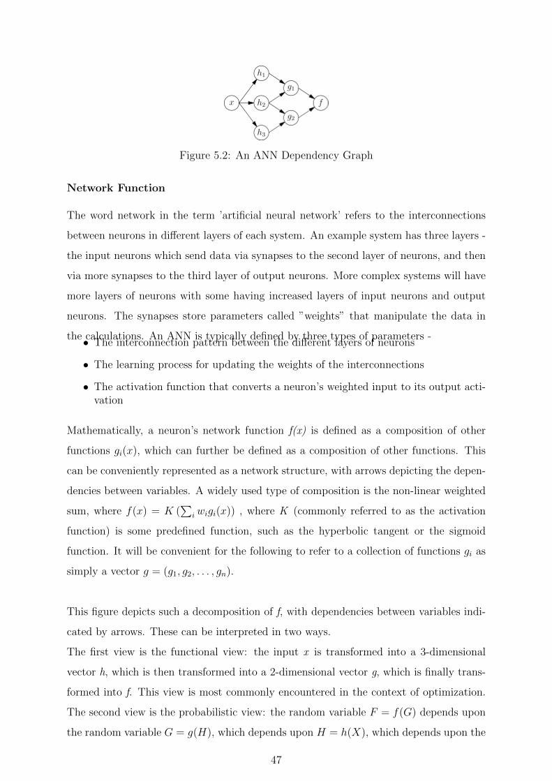
Figure 5.2: An ANN Dependency Graph

Network Function

The word network in the term ’artificial neural network’ refers to the interconnections

between neurons in different layers of each system. An example system has three layers -

the input neurons which send data via synapses to the second layer of neurons, and then

via more synapses to the third layer of output neurons. More complex systems will have

more layers of neurons with some having increased layers of input neurons and output

neurons. The synapses store parameters called ”weights” that manipulate the data in

the calculations. An ANN is typically defined by three types of parameters -• The interconnection pattern between the different layers of neurons

• The learning process for updating the weights of the interconnections

• The activation function that converts a neuron’s weighted input to its output acti-vation

Mathematically, a neuron’s network function f(x) is defined as a composition of other

functions gi(x), which can further be defined as a composition of other functions. This

can be conveniently represented as a network structure, with arrows depicting the depen-

dencies between variables. A widely used type of composition is the non-linear weighted

sum, where f(x) = K (∑

iwigi(x)) , where K (commonly referred to as the activation

function) is some predefined function, such as the hyperbolic tangent or the sigmoid

function. It will be convenient for the following to refer to a collection of functions gi as

simply a vector g = (g1, g2, . . . , gn).

This figure depicts such a decomposition of f, with dependencies between variables indi-

cated by arrows. These can be interpreted in two ways.

The first view is the functional view: the input x is transformed into a 3-dimensional

vector h, which is then transformed into a 2-dimensional vector g, which is finally trans-

formed into f. This view is most commonly encountered in the context of optimization.

The second view is the probabilistic view: the random variable F = f(G) depends upon

the random variable G = g(H), which depends upon H = h(X), which depends upon the

47

Figure 5.3: Two separate depictions of the recurrent ANN dependency graph

random variable X. This view is most commonly encountered in the context of graphical

models.

The two views are largely equivalent. In either case, for this particular network archi-

tecture, the components of individual layers are independent of each other (e.g. the

components of g are independent of each other given their input h). This naturally

enables a degree of parallelism in the implementation.

Networks such as the previous one are commonly called feedforward, because their graph

is a directed acyclic graph. Networks with cycles are commonly called recurrent. Such

networks are commonly depicted in the manner shown at the top of the figure, where f

is shown as being dependent upon itself. However, an implied temporal dependence is

not shown.

Learning

What has attracted the most interest in neural networks is the possibility of learning.

Given a specific task to solve, and a class of functions F , learning means using a set of

observations to find f ∗

in F which solves the task in some optimal sense. This entails defining a cost function

C : F → R such that, for the optimal solution f ∗, C(f ∗) ≤ C(f) ∀ f ∈ F i.e., no solution

has a cost less than the cost of the optimal solution.

The cost function C is an important concept in learning as it is a measure of how far

away a particular solution is from an optimal solution to the problem to be solved.

Learning algorithms search through the solution space to find a function that has the

smallest possible cost. For applications where the solution is dependent on some data,

the cost must necessarily be a function of the observations, otherwise we would not be

modelling anything related to the data. It is frequently defined as a statistic to which

only approximations can be made. As a simple example, consider the problem of finding

the model f , which minimizes C = E [(f(x)− y)2], for data pairs (x, y) drawn from some

distribution D. In practical situations we would only have N samples from D and thus,

48

for the above example, we would only minimize C = 1N

∑Ni=1(f(xi)− yi)2. Thus, the cost

is minimized over a sample of the data rather than the entire data set.

When N → ∞ some form of online machine learning must be used, where the cost is

partially minimized as each new example is seen. While online machine learning is often

used when D is fixed, it is most useful in the case where the distribution changes slowly

over time. In neural network methods, some form of online machine learning is frequently

used for finite datasets.

Choosing a Cost Function and Learning Algorithms

While it is possible to define some arbitrary ad-hoc cost function, frequently a partic-

ular cost will be used, either because it has desirable properties (such as convexity) or

because it arises naturally from a particular formulation of the problem (e.g., in a proba-

bilistic formulation the posterior probability of the model can be used as an inverse cost).

Ultimately, the cost function will depend on the desired task.

Training a neural network model essentially means selecting one model from the set of

allowed models (or, in a Bayesian framework, determining a distribution over the set of

allowed models) that minimizes the cost criterion. There are numerous algorithms avail-

able for training neural network models; most of them can be viewed as a straightforward

application of optimization theory and statistical estimation. Most of the algorithms

used in training artificial neural networks employ some form of gradient descent, using

back-propagation to compute the actual gradients. This is done by simply taking the

derivative of the cost function with respect to the network parameters and then changing

those parameters in a gradient-related direction. Evolutionary methods, gene expression

programming, simulated annealing, expectation-maximization, non-parametric methods

and particle swarm optimization are some commonly used methods for training neural

networks and these are beyond the scope of what we are implementing here.

5.1.3 Implementation of ANNs

Perhaps the greatest advantage of ANNs is their ability to be used as an arbitrary function

approximation mechanism that ’learns’ from observed data. However, using them is not so

straightforward, and a relatively good understanding of the underlying theory is essential.• Choice of model: This will depend on the data representation and the application.

Overly complex models tend to lead to problems with learning.

• Learning algorithm: There are numerous trade-offs between learning algorithms.

49

Almost any algorithm will work well with the correct hyperparameters for trainingon a particular fixed data set. However, selecting and tuning an algorithm fortraining on unseen data requires a significant amount of experimentation.

• Robustness: If the model, cost function and learning algorithm are selected appro-priately the resulting ANN can be extremely robust.

With the correct implementation, ANNs can be used naturally in online learning and

large data set applications. Their simple implementation and the existence of mostly

local dependencies exhibited in the structure allows for fast, parallel implementations in

hardware.

5.2 Convolutional Neural Networks - Feed-forward

ANNs

A Convolutional neural network (or CNN) is a type of feed-forward artificial neural net-

work where the individual neurons are tiled in such a way that they respond to overlapping

regions in the visual field. Convolutional networks were inspired by biological processes

and are variations of multilayer perceptrons which are designed to use minimal amounts

of preprocessing. In this major project, this approach is used to classify objects and faces

in image sequences.

5.2.1 Overview

When used for image recognition, convolutional neural networks (CNNs) consist of mul-

tiple layers of small neuron collections which look at small portions of the input image,

called receptive fields. The results of these collections are then tiled so that they overlap

to obtain a better representation of the original image; this is repeated for every such

layer. Because of this, they are able to tolerate translation of the input image. Convo-

lutional networks may include local or global pooling layers, which combine the outputs

of neuron clusters. They also consist of various combinations of convolutional layers and

fully connected layers, with point-wise non-linearity applied at the end of or after each

layer. It is inspired by biological process. To avoid the situation that there exist billions

of parameters if all layers are fully connected, the idea of using a convolution operation

on small regions, has been introduced. One major advantage of convolutional networks

is the use of shared weight in convolutional layers, which means that the same filter

50

(weights bank) is used for each pixel in the layer; this both reduces required memory size

and improves performance.

Some time-delay neural networks also use a very similar architecture to convolutional

neural networks, especially those for image recognition and/or classification tasks, since

the ”tiling” of the neuron outputs can easily be carried out in timed stages in a manner

useful for analysis of images.

Compared to other image classification algorithms, convolutional neural networks use

relatively little pre-processing. This means that the network is responsible for learning

the filters that in traditional algorithms were hand-engineered. The lack of a dependence

on prior-knowledge and the existence of difficult to design hand-engineered features is a

major advantage for CNNs.

5.2.2 Modelling the CNN and it’s different layers

When doing propagation, the momentum and weight decay are introduced to avoid much

oscillation during stochastic gradient descent.

Convolutional Layer

Unlike a hand-coded convolution kernel (Sobel, Prewitt, Roberts), in a convolutional

neural net, the parameters of each convolution kernel are trained by the backpropagation

algorithm. There are many convolution kernels in each layer, and each kernel is replicated

over the entire image with the same parameters. The function of the convolution operators

is to extract different features of the input. The capacity of a neural net varies, depending

on the number of layers. The first convolution layers will obtain the low-level features,

like edges, lines and corners. The more layers the network has, the higher-level features

it will get.

ReLU Layer

ReLU is the abbreviation of Rectified Linear Units, which is a name for neurons using

the non-saturating activation function f(x) = max(0, x), also called the positive part. It

is used to increase the non-linear properties of a network as well as the decision function

without affecting the receptive fields of the convolution layer.

There are many other used functions to increase nonlinearity, for example the saturating

hyperbolic tangent f(x) = tanh(x), f(x) = |tanh(x)|, and the sigmoid function f(x) =

51

(1 + e−x)−1. The advantage of ReLU compared to tanh units is that with it, the neural

network trains several times faster.

Pooling Layer

In order to reduce variance, pooling layers compute the maximum or average value of a

particular feature over a region of the image. This will ensure that the same result will

be obtained, even when image features have small translations. This is an important

operation for object classification and detection.

Dropout Layer

Since a fully connected layer occupies most of the parameters, over-fitting can happen

easily. The dropout method is introduced to prevent over-fitting. Dropout also signifi-

cantly improves the speed of training. This makes model combination practical, even for

deep neural nets. Dropout is performed randomly. In the input layer, the probability

of dropping a neuron is between 0.5 and 1, while in the hidden layers, a probability of

0.5 is used. The neurons that are dropped out, will not contribute to the forward pass

and back propagation. This is equivalent to decreasing the number of neurons. This will

create neural networks with different architectures, but all of those networks will share

the same weights.

The biggest contribution of the dropout method is that, although it effectively generates

2n neural nets, with different architectures (n =number of ”droppable” neurons), and

as such, allows for model combination, at test time, only a single network needs to be

tested. This is accomplished by performing the test with the un-thinned network, while

multiplying the output weights of each neuron with the probability of that neuron being

retained (i.e. not dropped out).

Loss Layer

It can use different loss functions for different tasks. Softmax loss is used for predicting

a single class of K mutually exclusive classes. Sigmoid cross-entropy loss is used for

predicting K independent probability values in [0,1]. Euclidean loss is used for regressing

to real-valued lables [-inf,inf]

52

5.2.3 Common Libraries Used for CNNs

The following libraries are very commonly used for the creation and application of CNNs

in object recognition.• Caffe: Caffe (replacement of Decaf) has been the most popular libraries for Convo-

lutional neural networks. It is created by the Berkeley Vision and Learning Center(BVLC). The advantages are that it has cleaner architecture and faster speed. Itsupports both CPU and GPU, easily switching them. It is developed in C++, andhas python and Matlab wrappers. In the developing of caffe, protobuf is used tomake researchers tune the parameters easily as well as adding or removing layers.

• Torch7 (www.torch.ch)

• OverFeat

• Cuda-convnet

• MatConvnet

• Theano: written in python, using scientific python

5.2.4 Results of using a CNN for Object Recognition

As an exercise, we looked at implementing a convolutional neural network for the problem

statement given in the Stanford UFLDL Tutorial. It involved the modification of the

cnnConvolve.m and cnnPool.m codes for the extraction of features on 8X8 patches of

a reduced STL-10 dataset by applying convolution and pooling. The reduced STL-10

dataset comprised of 64x64 images from 4 classes (aeroplane, car, cat, dog) We wrote

the code in Python using Scipy, Numpy and Matplotlib and is currently bounded by the

MIT License (MIT).

For compiling the code, we had to download the data files - ′stlT rainSubset.mat′,

′stlTestSubset.mat′, ′optparam.npy′, ′zcawhite.npy′ and ′meanpatch.npy′ and the code

file ′convolutionalNeuralNetwork.py′ and place them in the same folder. We ran the

′convolutionalNeuralNetwork.py′ code in the command line. We first got an image of

the learned Sparse Auto-Encoder Linear Weights as suggested in the ′output.png′, the

code for which was written by us. The data files ′optparam.npy′, ′zcawhite.npy′ and

′meanpatch.npy′ were also obtained using the same code that we wrote and the results

for the same are shown above. The code took around an hour to execute on an I-5

processor.

53

Figure 5.4: Features obtained from the reduced STL-10 dataset by applying Convolutionand Pooling

5.3 Recurrent Neural Networks - Cyclic variants of

ANNs

A recurrent neural network (RNN) is a class of artificial neural network where connections

between units form a directed cycle. This creates an internal state of the network which

allows it to exhibit dynamic temporal behaviour. Unlike feed-forward neural networks,

RNNs can use their internal memory to process arbitrary sequences of inputs. Each of

these RNNs have their own associates architectures and we will be highlighting a few of

these here. We will then highlight the training methods for such a network and then talk

about modelling such networks.

5.3.1 RNN Architectures

Fully Recurrent Network

This is the basic architecture developed: a network of neuron-like units, each with a

directed connection to every other unit. Each unit has a time-varying real-valued activa-

tion. Each connection has a modifiable real-valued weight. Some of the nodes are called

input nodes, some output nodes, the rest hidden nodes. Most architectures below are

special cases.

For supervised learning in discrete time settings, training sequences of real-valued input

vectors become sequences of activations of the input nodes, one input vector at a time.

At any given time step, each non-input unit computes its current activation as a non-

linear function of the weighted sum of the activations of all units from which it receives

54

connections. There may be teacher-given target activations for some of the output units

at certain time steps. For example, if the input sequence is a speech signal correspond-

ing to a spoken digit, the final target output at the end of the sequence may be a label

classifying the digit. For each sequence, its error is the sum of the deviations of all target

signals from the corresponding activations computed by the network. For a training set

of numerous sequences, the total error is the sum of the errors of all individual sequences.

Algorithms for minimizing this error are mentioned in the section on training algorithms

below.

In reinforcement learning settings, there is no teacher providing target signals for the

RNN, instead a fitness function or reward function is occasionally used to evaluate the

RNN’s performance, which is influencing its input stream through output units connected

to actuators affecting the environment. Again, compare the section on training algorithms

below.

Elman Networks and Jordan Networks

This special case of the basic architecture above was employed by Jeff Elman. A three-

layer network is used (arranged vertically as x, y, and z in the illustration), with the

addition of a set of ”context units” (u in the illustration). There are connections from

the middle (hidden) layer to these context units fixed with a weight of one. At each time

step, the input is propagated in a standard feed-forward fashion, and then a learning rule

is applied. The fixed back connections result in the context units always maintaining a

copy of the previous values of the hidden units (since they propagate over the connections

before the learning rule is applied). Thus the network can maintain a sort of state,

allowing it to perform such tasks as sequence-prediction that are beyond the power of a

standard multilayer perceptron.

Jordan networks, due to Michael I. Jordan, are similar to Elman networks. The context

units are however fed from the output layer instead of the hidden layer. The context

units in a Jordan network are also referred to as the state layer, and have a recurrent

connection to themselves with no other nodes on this connection. Elman and Jordan

networks are also known as ”simple recurrent networks” (SRN).

Long Short Term Networks

The Long short term memory (LSTM) network, developed by Hochreiter and Schmid-

huber is an artificial neural net structure that unlike traditional RNNs doesn’t have the

55

Figure 5.5: An Elman SRNN

56

vanishing gradient problem (compare the section on training algorithms below). It works

even when there are long delays, and it can handle signals that have a mix of low and

high frequency components. LSTM RNN outperformed other methods in numerous ap-

plications such as language learning and connected handwriting recognition and this is

precisely why we are using this architecture for associating a description for our images.

Continuous Time RNNs

A continuous time recurrent neural network (CTRNN) is a dynamical systems model of

biological neural networks. A CTRNN uses a system of ordinary differential equations to

model the effects on a neuron of the incoming spike train. CTRNNs are more computa-

tionally efficient than directly simulating every spike in a network as they do not model

neural activations at this level of detail.

For a neuron i in the network with action potential yi the rate of change of activation is

given by:

τiyi = −yi + σ(∑n

j=1wjiyj −Θj) + Ii(t)

where:

τi : Time constant of post-synaptic node yi : Activation of post-synaptic node yi : Rate

of change of activation of post-synaptic node wji : Weight of connection from pre to

post-synaptic node σ(x) : Sigmoid of x e.g. σ(x) = 1/(1 + e−x) yj : Activation of

pre-synaptic node Θj : Bias of pre-synaptic node Ii(t) : Input (if any) to node

CTRNNs have frequently been applied in the field of evolutionary robotics, where they

have been used to address, for example, vision, co-operation and minimally cognitive

behaviour.

5.3.2 Training an RNN

Gradient Descent

To minimize total error, gradient descent can be used to change each weight in propor-

tion to the derivative of the error with respect to that weight, provided the non-linear

activation functions are differentiable. Various methods for doing so were developed by

Paul Werbos, Ronald J. Williams, Tony Robinson, Jrgen Schmidhuber, Sepp Hochreiter,

Barak Pearlmutter, and others.

57

The standard method is called ”backpropagation through time” or BPTT, and is a gen-

eralization of back-propagation for feed-forward networks, and like that method, is an

instance of Automatic differentiation in the reverse accumulation mode or Pontryagin’s

minimum principle. A more computationally expensive online variant is called ”Real-

Time Recurrent Learning” or RTRL, which is an instance of Automatic differentiation

in the forward accumulation mode with stacked tangent vectors. Unlike BPTT this al-

gorithm is local in time but not local in space.

There also is an online hybrid between BPTT and RTRL with intermediate complexity,

and there are variants for continuous time. A major problem with gradient descent for

standard RNN architectures is that error gradients vanish exponentially quickly with the

size of the time lag between important events. The Long short term memory architecture

together with a BPTT/RTRL hybrid learning method was introduced in an attempt to

overcome these problems.

Global Optimization Methods

Training the weights in a neural network can be modelled as a non-linear global opti-

mization problem. A target function can be formed to evaluate the fitness or error of a

particular weight vector as follows: First, the weights in the network are set according to

the weight vector. Next, the network is evaluated against the training sequence. Typi-

cally, the sum-squared-difference between the predictions and the target values specified

in the training sequence is used to represent the error of the current weight vector. Arbi-

trary global optimization techniques may then be used to minimize this target function.

The most common global optimization method for training RNNs is genetic algorithms,

especially in unstructured networks.

Initially, the genetic algorithm is encoded with the neural network weights in a predefined

manner where one gene in the chromosome represents one weight link, henceforth; the

whole network is represented as a single chromosome. The fitness function is evaluated as

follows: 1) each weight encoded in the chromosome is assigned to the respective weight

link of the network ; 2) the training set of examples is then presented to the network

which propagates the input signals forward ; 3) the mean-squared-error is returned to the

fitness function; 4) this function will then drive the genetic selection process.

There are many chromosomes that make up the population; therefore, many different

neural networks are evolved until a stopping criterion is satisfied. A common stopping

58

scheme is: 1) when the neural network has learnt a certain percentage of the training

data or 2) when the minimum value of the mean-squared-error is satisfied or 3) when the

maximum number of training generations has been reached. The stopping criterion is

evaluated by the fitness function as it gets the reciprocal of the mean-squared-error from

each neural network during training. Therefore, the goal of the genetic algorithm is to

maximize the fitness function, hence, reduce the mean-squared-error.

Other global (and/or evolutionary) optimization techniques may be used to seek a good

set of weights such as Simulated annealing or Particle swarm optimization.

5.4 Deep Visual-Semantic Alignments for generating

Image Descriptions - CNN + RNN

After having clearly understood how CNNs and RNNs work, we looked towards describ-

ing our image sequences and using a certain set of key words to monitor a malicious

activity. Our current work is on the alignment of such visual and semantic data for

describing images using the multi-modal approach. The model that we are trying to

implement leverages datasets of images and their sentence descriptions to learn about

the inter-modal correspondences between text and visual data. Our approach is based

on a combination of Convolutional Neural Networks over image regions, bidirectional

Recurrent Neural Networks over sentences, and a structured objective that aligns the

two modalities through a multi-modal embedding. We then describe a Recurrent Neural

Network architecture (the LSTM architecture discussed earlier) that uses the inferred

alignments to learn to generate novel descriptions of image regions. We are looking

to demonstrate the effectiveness of our alignment model with ranking experiments on

Flickr8K, Flickr30K and MSCOCO datasets.

5.4.1 The Approach

A quick glance at an image is sufficient for a human to point out and describe an immense

amount of details about the visual scene. However, this remarkable ability has proven to

be an elusive task for our visual recognition models. The majority of previous work in

visual recognition has focused on labelling images with a fixed set of visual categories,

and great progress has been achieved in these endeavours. However, while closed vocab-

ularies of visual concepts constitute a convenient modelling assumption, they are vastly

59

Figure 5.6: Generating a free-form natural language descriptions of image regions

restrictive when compared to the enormous amount of rich descriptions that a human

can compose.

Some pioneering approaches that address the challenge of generating image descriptions

have been developed. However, these models often rely on hard-coded visual concepts

and sentence templates, which imposes limits on their variety. Moreover, the focus of

these works has been on reducing complex visual scenes into a single sentence, which we

consider as an unnecessary restriction.

In the next few weeks, we strive to take a step towards the goal of generating dense, free-

form descriptions of images as shown in the above figure. The primary challenge towards

this goal is in the design of a model that is rich enough to reason simultaneously about

contents of images and their representation in the domain of natural language. Addition-

ally, the model should be free of assumptions about specific hard-coded templates, rules

or categories and instead rely primarily on training data. The second, practical challenge

is that datasets of image captions are available in large quantities on the internet, but

these descriptions multiplex mentions of several entities whose locations in the images

are unknown.

Our core insight is that we can leverage these large image-sentence datasets by treating

the sentences as weak labels, in which contiguous segments of words correspond to some

particular, but unknown location in the image. Our approach is to infer these alignments

and use them to learn a generative model of descriptions. Concretely, the ideas are

two-fold:• We develop a deep neural network model that infers the latent alignment betweensegments of sentences and the region of the image that they describe. The modelis supposed to associate the two modalities through a common, multi-modal em-bedding space and a structured objective. We will validate the effectiveness of thisapproach on image-sentence retrieval experiments.

60

Figure 5.7: An Overview of the approach

• We then look towards introducing a multi-modal Recurrent Neural Network archi-tecture that takes an input image and generates its description in text. We trainthe model on the inferred correspondences and evaluate its performance on a newdataset of region-level annotations.

5.4.2 Modelling such a Network

The ultimate goal of our model is to generate descriptions of image regions. During

training, the input to our model is a set of images and their corresponding sentence

descriptions as shown in the above figure. We first present a model that aligns segments

of sentences to the visual regions that they describe through a multi-modal embedding.

We then treat these correspondences as training data for our multi-modal Recurrent

Neural Network model which learns to generate the descriptions.

Learning to Align Visual and Language data

Our alignment model assumes an input dataset of images and their sentence descriptions.

The key challenge to inferring the association between visual and textual data is that

sentences written by people make multiple references to some particular, but unknown

locations in the image. For example, in the above figure, the words Tabby cat is leaning

refer to the cat, the words wooden table refer to the table, etc.

We would like to infer these latent correspondences, with the goal of later learning to

generate these snippets from image regions. We build on the basic approach of Karpathy

et al., who learn to ground dependency tree relations in sentences to image regions as part

of a ranking objective. We look towards the use of bidirectional recurrent neural networks

to compute word representations in the sentence, dispensing of the need to compute

dependency trees and allowing unbounded interactions of words and their context in the

sentence. We also substantially simplify their objective and show that both modifications

improve ranking performance.

We first describe neural networks that map words and image regions into a common,

multimodal embedding. Then we introduce our objective, which learns the embedding

61

representations so that semantically similar concepts across the two modalities occupy

nearby regions of the space.

The idea and the mathematics behind the model are currently being looked into and a

preliminary analysis of the same has been presented below:

Representing Images

Following prior work, we observe that sentence descriptions make frequent references to

objects and their attributes. Thus, we follow the method of Girshick et al. to detect

objects in every image with a Region Convolutional Neural Network (RCNN). The CNN

is pre-trained on ImageNet and fine tuned on the 200 classes of the ImageNet Detection

Challenge. To establish fair comparisons to Karpathy et al., we use the top 19 detected

locations and the whole image and compute the representations based on the pixels Ib

inside each bounding box as follows:

v = Wm[CNNθc(Ib)] + bm

where CNN(Ib) transforms the pixels inside the bounding box Ib into 4096-dimensional

activations of the fully connected layer immediately before the classifier. The CNN pa-

rameters θc contain approximately 60 million parameters and the architecture closely

follows the network of Krizhevsky et al. The matrix Wm has dimensions h× 4096, where

h is the size of the multi-modal embedding space (h currently ranges from 1000-1600

in our experiments). Every image is thus represented as a set of h-dimensional vectors

vi|i = 1...20

Representing Sentences

To establish the inter-modal relationships, we would like to represent the words in the

sentence in the same h-dimensional embedding space that the image regions occupy. The

simplest approach might be to project every individual word directly into this embedding.

However, this approach does not consider any ordering and word context information in

the sentence. An extension to this idea is to use word bi-grams, or dependency tree

relations as previously proposed. However, this still imposes an arbitrary maximum size

of the context window and requires the use of Dependency Tree Parsers that might be

trained on unrelated text corpora.

To address these concerns, we look towards using a bidirectional recurrent neural network

(BRNN) to compute the word representations. In our setting, the BRNN takes a sequence

of N words (encoded in a 1-of-k representation) and transforms each one into an h-

dimensional vector. However, the representation of each word is enriched by a variably-

62

sized context around that word. Using the index t = 1....N to denote the position of a

word in a sentence, the form of the BRNN we are looking to use is as follows:

xt = Wwπt

et = f(Wext + be)

hft = f(et +Wfhft−1 + bf )

hbt = f(et +Wbhbt+1 + bb)

st = f(Wdhft + hbt + bd)

Here, πt is an indicator column vector that is all zeros except for a single one at the

index of the tth word in a word vocabulary. The weights Ww specify a word embedding

matrix that we initialize with a 300-dimensional word2vec weights and keep fixed in

our experiments due to over-fitting concerns. Note that the B-RNN consists of two

independent streams of processing, one moving left to right (hft ) and the other right to

left (hbt). The final h-dimensional representation st for the tth word is a function of both

the word at that location and also its surrounding context in the sentence. Technically,

every st is a function of all words in the entire sentence, but our empirical finding is that

the final word representations (st) align most strongly to the visual concept of the word

at that location (πt). Our hypothesis is that the strength of influence diminishes with

each step of processing since st is a more direct function of πt than of the other words in

the sentence.

We learn the parameters We,Wf ,Wb,Wd and the respective biases be, bf , bb, bd. A typical

size of the hidden representation in our experiments ranges between 300-600 dimensions.

We set the activation function f to the rectified linear unit (ReLU), which computes

f : x→ max(0, x).

Alignment Objective

We have described the transformations that map every image and sentence into a set

of vectors in a common h-dimensional space. Since our labels are at the level of entire

images and sentences, our strategy is to formulate an image-sentence score as a function

of the individual scores that measure how well a word aligns to a region of an image.

Intuitively, a sentence-image pair should have a high matching score if its words have a

63

Figure 5.8: Evaluating the Image-Sentence Score

confident support in the image. In Karpathy et al., they interpreted the dot product vTi st

between an image fragment i and a sentence fragment t as a measure of similarity and

used these to define the score between image k and sentence l as:

Skl = Σt∈glΣi∈gkmax(0, vTi st)

Here, gk is the set of image fragments in image k and gl is the set of sentence fragments

in sentence l. The indices k, l range over the images and sentences in the training set.

Together with their additional Multiple Instance Learning objective, this score carries the

interpretation that a sentence fragment aligns to a subset of the image regions whenever

the dot product is positive. We found that the following reformulation simplifies the

model and alleviates the need for additional objectives and their hyper-parameters:

Skl = Σt∈glmaxi∈gkvTi st

Here, every word st aligns to the single best image region. As we show in the experiments,

this simplified model also leads to improvements in the final ranking performance. As-

suming that k = l denotes a corresponding image and sentence pair, the final max-margin,

structured loss remains:

C(θ) = Σk[Σlmax(0, Skl − Skk + 1) + Σlmax(0, Slk − Skk + 1)]

This objective encourages aligned image-sentences pairs to have a higher score than mis-

aligned pairs, by a margin.

Decoding text segment alignments to images

64

Consider an image from the training set and its corresponding sentence. We can interpret

the quantity vTi st as the un-normalized log probability of the tth word describing any of the

bounding boxes in the image. However, since we are ultimately interested in generating

snippets of text instead of single words, we would like to align extended, contiguous

sequences of words to a single bounding box. Note that the nave solution that assigns

each word independently to the highest-scoring region is insufficient because it leads to

words getting scattered inconsistently to different regions.

To address this issue, we treat the true alignments as latent variables in a Markov Random

Field (MRF) where the binary interactions between neighbouring words encourage an

alignment to the same region. Concretely, given a sentence with N words and an image

with M bounding boxes, we introduce the latent alignment variables aj ∈ 1...M for

j = 1...N and formulate an MRF in a chain structure along the sentence as follows:

E(a) = Σj=1...NψUj (aj) + Σj=1..N−1ψ

Bj (aj, aj+1)

ψUj (aj = t) = vTi st

ψBj (aj, aj+1) = βπ[aj = aj+1]

Here, β is a hyperparameter that controls the affinity towards longer word phrases. This

parameter allows us to interpolate between single-word alignments (β = 0) and aligning

the entire sentence to a single, maximally scoring region when β is large. We minimize

the energy to find the best alignments a using dynamic programming. The output of this

process is a set of image regions annotated with segments of text.

Idea of a Multi-Modal RNN for generating descriptions

In this section, we assume an input set of images and their textual descriptions. These

could be full images and their sentence descriptions, or regions and text snippets as dis-

cussed in previous sections. The key challenge is in the design of a model that can predict

a variable-sized sequence of outputs. In previously developed language models based on

Recurrent Neural Networks (RNNs), this is achieved by defining a probability distribu-

tion of the next word in a sequence, given the current word and context from previous

time steps. We explore a simple but effective extension that additionally conditions the

generative process on the content of an input image. More formally, the RNN takes the

image pixels I and a sequence of input vectors (x1, ..., xT ). It then computes a sequence

65

Figure 5.9: Diagram of the multi-modal Recurrent Neural Network generative model

of hidden states (h1, ..., ht) and a sequence of outputs (y1, ..., yt) by iterating the following

recurrence relation for t = 1toT :

bv = Whi[CNNθc(I)]

ht = f(Whxxt +Whhht1 + bh + bv)

yt = softmax(Wohht + bo)

In the equations above, Whi, Whx, Whh, Woh and bh, bo are a set of learnable weights

and biases. The output vector yt has the size of the word dictionary and one additional

dimension for a special END token that terminates the generative process. Note that we

provide the image context vector bv to the RNN at every iteration so that it does not

have to remember the image content while generating words.

RNN Training

The RNN is trained to combine a word (xt), the previous context (ht1) and the image

information (bv) to predict the next word (yt). Concretely, the training proceeds as follows

(refer the above figure): We set h0 = 0, x1 to a special START vector, and the desired

label y1 as the first word in the sequence. In particular, we use the word embedding for

the as the START vector x1. Analogously, we set x2 to the word vector of the first word

and expect the network to predict the second word, etc. Finally, on the last step when

xT represents the last word, the target label is set to a special END token. The cost

function is to maximize the log probability assigned to the target labels.

RNN Testing

The RNN predicts a sentence as follows: We compute the representation of the image bv,

set h0 = 0, x1 to the embedding of the word the, and compute the distribution over the

first word y1. We sample from the distribution (or pick the argmax), set its embedding

vector as x2, and repeat this process until the END token is generated.

66

Optimization

We use the Stochastic Gradient Descent with mini-batches of 100 image-sentence pairs

and momentum of 0.9 to optimize the alignment model. We cross-validate the learning

rate and the weight decay. We also use drop-out regularization in all layers except in

the recurrent layers. The generative RNN is more difficult to optimize, partly due to

the word frequency disparity between rare words, and very common words (such as the

END token). We achieved the best results using RMSprop, which is an adaptive step

size method that scales the gradient of each weight by a running average of its gradient

magnitudes.

5.5 Results

We are working towards achieving image description using the Flickr8k, Flickr30k and

MSCOCO Datasets. The MSCOCO checkpoint model describes our test images the

best, and hence we finalised on using the same model to test other images too to predict

sentences. However, the time complexity for extracting the features and running the

neural network was really huge. The time for calculation of CNN features for a batch

of 10 images was approximately 25 seconds while running on a normal CPU. We are

estimating that running the same neural network on a GPU would reduce computational

resources and hence, computational time by at least 2 times the speed on CPU due to

parallel architectures. However, we were unable to run in on the GPU because we didn’t

have the resources. Also, the RNN takes a further 5 seconds to process to generate

linguistic equivalents of the image.

67

CHAPTER 6Database Management System using MongoDB for

Face and Object Recognition

Our database management system was developed as part of the facial and object recog-

nition portion of our project using MongoDB. The idea behind implementing such a

database is to sort through all the data through proper indexing of material for each

person. MongoDB is an open-source document database that provides high performance,

high availability, and automatic scaling. A record in MongoDB is a document, which is

a data structure composed of field and value pairs. MongoDB documents are similar to

JSON objects. The values of fields may include other documents, arrays, and arrays of

documents.

6.1 Introduction

It is often said that technology moves at a blazing pace. Its true that there is an ever

growing list of new technologies and techniques being released. However, weve long been

of the opinion that the fundamental technologies used by programmers move at a rather

slow pace. One could spend years learning little yet remain relevant. What is striking

though is the speed at which established technologies get replaced. Seemingly overnight,

long-established technologies find themselves threatened by shifts in developer focus.

The first thing we ought to do is explain what is meant by NoSQL. Its a broad term that

means different things to different people. Personally, we use it very broadly to mean a

system that plays a part in the storage of data. Put another way, NoSQL (again, for us), is

the belief that your persistence layer isnt necessarily the responsibility of a single system.

Where relational database vendors have historically tried to position their software as a

one-size-fits-all solution, NoSQL leans towards smaller units of responsibility where the

best tool for a given job can be leveraged. So, your NoSQL stack might still leverage a

relational database, say MySQL, but itll also contain Redis as a persistence lookup for

specific parts of the system as well as Hadoop for your intensive data processing. Put

simply, NoSQL is about being open and aware of alternative, existing and additional

patterns and tools for managing your data.

You might be wondering where MongoDB fits into all of this. As a document-oriented

database, MongoDB is a more generalized NoSQL solution. It should be viewed as an

Figure 6.1: A MongoDB Document

alternative to relational databases. Like relational databases, it too can benefit from

being paired with some of the more specialized NoSQL solutions.

6.2 CRUD Operations

MongoDB provides rich semantics for reading and manipulating data. CRUD stands

for create, read, update, and delete. These terms are the foundation for all interactions

with the database. MongoDB stores data in the form of documents, which are JSON-like

field and value pairs. Documents are analogous to structures in programming languages

that associate keys with values (e.g. dictionaries, hashes, maps, and associative arrays).

Formally, MongoDB documents are BSON documents. BSON is a binary representation

of JSON with additional type information. In the documents, the value of a field can be

any of the BSON data types, including other documents, arrays, and arrays of documents.

MongoDB stores all documents in collections. A collection is a group of related documents

that have a set of shared common indexes. Collections are analogous to a table in

relational databases.

6.2.1 Database Operations

Query

In MongoDB a query targets a specific collection of documents. Queries specify criteria,

or conditions, that identify the documents that MongoDB returns to the clients. A query

may include a projection that specifies the fields from the matching documents to return.

You can optionally modify queries to impose limits, skips, and sort orders.

69

Figure 6.2: A MongoDB Collection of Documents

Data Modification

Data modification refers to operations that create, update, or delete data. In MongoDB,

these operations modify the data of a single collection. For the update and delete oper-

ations, you can specify the criteria to select the documents to update or remove.

6.2.2 Related Features

Indexes

To enhance the performance of common queries and updates, MongoDB has full support

for secondary indexes. These indexes allow applications to store a view of a portion of

the collection in an efficient data structure. Most indexes store an ordered representation

of all values of a field or a group of fields. Indexes may also enforce uniqueness, store

objects in a geo-spatial representation, and facilitate text search.

Replica Set Read Preference

For replica sets and sharded clusters with replica set components, applications specify

read preferences. A read preference determines how the client direct read operations to

the set.

Write Concern

Applications can also control the behaviour of write operations using write concern.

Particularly useful for deployments with replica sets, the write concern semantics allow

clients to specify the assurance that MongoDB provides when reporting on the success

70

Figure 6.3: Components of a MongoDB Find Operation

of a write operation.

Aggregation

In addition to the basic queries, MongoDB provides several data aggregation features. For

example, MongoDB can return counts of the number of documents that match a query,

or return the number of distinct values for a field, or process a collection of documents

using a versatile stage-based data processing pipeline or map-reduce operations.

6.2.3 Read Operations

Read operations, or queries, retrieve data stored in the database. In MongoDB, queries

select documents from a single collection. Queries specify criteria, or conditions, that

identify the documents that MongoDB returns to the clients. A query may include a

projection that specifies the fields from the matching documents to return. The projection

limits the amount of data that MongoDB returns to the client over the network.

Query Interface

For query operations, MongoDB provides a db.collection.find() method. The method

accepts both the query criteria and projections and returns a cursor to the matching

documents. We can optionally modify the query to impose limits, skips, and sort orders.

The following diagram highlights the components of a MongoDB query operation:

Query Statements

Consider the following diagram of the query process that specifies a query criteria and

a sort modifier: In the diagram, the query selects documents from the users collection.

Using a query selection operator to define the conditions for matching documents, the

query selects documents that have age greater than (i.e. $ gt)18. Then the sort() modifier

sorts the results by age in ascending order.

71

Figure 6.4: Stages of a MongoDB query with a query criteria and a sort modifier

6.2.4 Write Operations

A write operation is any operation that creates or modifies data in the MongoDB instance.

In MongoDB, write operations target a single collection. All write operations in MongoDB

are atomic on the level of a single document. There are three classes of write operations

in MongoDB: insert, update, and remove.

Insert (Create) operations add new data to a collection. Update operations modify ex-

isting data, and remove operations delete data from a collection. No insert, update, or

remove can affect more than one document atomically. For the update and remove op-

erations, you can specify criteria, or conditions, that identify the documents to update

or remove. These operations use the same query syntax to specify the criteria as read

operations. MongoDB allows applications to determine the acceptable level of acknowl-

edgement required of write operations.

Insert (Create)

In MongoDB, the db.collection.insert() method adds new documents to a collection. The

following diagram highlights the components of a MongoDB insert operation:

Update

In MongoDB, the db.collection.update() method modifies existing documents in a collec-

tion. The db.collection.update() method can accept query criteria to determine which

documents to update as well as an options document that affects its behaviour, such as

the multi option to update multiple documents. The following diagram highlights the

72

Figure 6.5: Components of a MongoDB Insert Operation

Figure 6.6: Components of a MongoDB Update Operation

components of a MongoDB update operation:

Default Update Behaviour: By default, the db.collection.update() method updates

a single document. However, with the multi option, update() can update all documents

in a collection that match a query. The db.collection.update() method either updates

specific fields in the existing document or replaces the document. When performing

update operations that increase the document size beyond the allocated space for that

document, the update operation relocates the document on disk. MongoDB preserves

the order of the document fields following write operations except for the following cases:• The id field is always the first field in the document.

• Updates that include renaming of field names may result in the reordering of fieldsin the document.

In version 2.6, MongoDB actively attempts to preserve the field order in a document.

Before version 2.6, MongoDB did not actively preserve the order of the fields in a docu-

ment.

Update Behavior with the upsert Option: If the update() method includes upsert:

true and no documents match the query portion of the update operation, then the update

operation creates a new document. If there are matching documents, then the update

operation with the upsert: true modifies the matching document or documents.

By specifying upsert: true, applications can indicate, in a single operation, that if no

matching documents are found for the update, an insert should be performed.

73

Figure 6.7: Components of a MongoDB Remove Operation

Remove (Delete)

In MongoDB, the db.collection.remove() method deletes documents from a collection.

The db.collection.remove() method accepts a query criteria to determine which doc-

uments to remove. The following diagram highlights the components of a MongoDB

remove operation:

6.3 Indexing

Indexes support the efficient execution of queries in MongoDB. Without indexes, Mon-

goDB must scan every document in a collection to select those documents that match

the query statement. These collection scans are inefficient because they require mongod

to process a larger volume of data than an index for each operation.

Indexes are special data structures that store a small portion of the collections data set

in an easy to traverse form. The index stores the value of a specific field or set of fields,

ordered by the value of the field. Fundamentally, indexes in MongoDB are similar to

indexes in other database systems. MongoDB defines indexes at the collection level and

supports indexes on any field or sub-field of the documents in a MongoDB collection. If

an appropriate index exists for a query, MongoDB can use the index to limit the number

of documents it must inspect. In some cases, MongoDB can use the data from the index

to determine which documents match a query. The following diagram illustrates a query

that selects documents using an index.

6.3.1 Optimization

Create indexes to support common and user-facing queries. Having these indexes will

ensure that MongoDB only scans the smallest possible number of documents. Indexes

can also optimize the performance of other operations in specific situations:

74

Figure 6.8: A query that uses an index to select and return sorted results

Figure 6.9: A query that uses only the index to match the query criteria and return theresults

Sorted Results

MongoDB can use indexes to return documents sorted by the index key directly from the

index without requiring an additional sort phase.

Covered Results

When the query criteria and the projection of a query include only the indexed fields,

MongoDB will return results directly from the index without scanning any documents or

bringing documents into memory. These covered queries can be very efficient.

6.3.2 Index Types

MongoDB provides a number of different index types to support specific types of data

and queries.

75

Figure 6.10: An index on the ”score” field (ascending)

Default id

All MongoDB collections have an index on the id field that exists by default. If appli-

cations do not specify a value for id the driver or the mongod will create an id field

with an ObjectId value. The id index is unique, and prevents clients from inserting two

documents with the same value for the id field.

Single Field

In addition to the MongoDB-defined id index, MongoDB supports user-defined indexes

on a single field of a document. Consider the following illustration of a single-field index:

Compound Index

MongoDB also supports user-defined indexes on multiple fields. These compound indexes

behave like single-field indexes; however, the query can select documents based on addi-

tional fields. The order of fields listed in a compound index has significance. For instance,

if a compound index consists of userid : 1, score : −1, the index sorts first by userid and

then, within each userid value, sort by score. Consider the following illustration of this

compound index:

Multikey Index

MongoDB uses multikey indexes to index the content stored in arrays. If you index a field

that holds an array value, MongoDB creates separate index entries for every element of

the array. These multikey indexes allow queries to select documents that contain arrays

by matching on element or elements of the arrays. MongoDB automatically determines

whether to create a multikey index if the indexed field contains an array value; you do

76

Figure 6.11: A compound index on the ”userid” field (ascending) and the ”score” field(descending)

Figure 6.12: A Multikey index on the addr.zip field

not need to explicitly specify the multikey type. Consider the following illustration of a

multikey index:

Geospatial Index

To support efficient queries of geospatial coordinate data, MongoDB provides two special

indexes: 2d indexes that uses planar geometry when returning results and 2sphere indexes

that use spherical geometry to return results.

Text Indexes

MongoDB provides a text index type that supports searching for string content in a

collection. These text indexes do not store language-specific stop words (e.g. the, a, or)

and stem the words in a collection to only store root words.

77

Figure 6.13: Finding an individual’s image using the unique ID

Hashed Indexes

To support hash based sharding, MongoDB provides a hashed index type, which indexes

the hash of the value of a field. These indexes have a more random distribution of values

along their range, but only support equality matches and cannot support range-based

queries.

6.4 Results

We have currently established a working database that contains the necessary documents

for each person. Their images are stored as a document of 2-D arrays. A screen-shot

of scripting on the database environment ”RoboMongo” has been provided below. They

showcase the image document of each person as well as their respective background data.

78

Figure 6.14: Background Data corresponding to each individual

79

CHAPTER 7

Final Results, Issues Faced and Future Improvements

7.1 Final Algorithm

The algorithm to detect a malicious activity based on real time video acquisition has been

implemented. It is pretty straightforward and simple. We first acquire the video and

process only one frame in a span of 10 frames so that we give enough time for the frame

to get processed. We then detect the presence of a malicious object using HOG features

as suggested in Chapter 4 and then further if a malicious activity is not detected, we go

towards the implementation of the multi-modal approach towards semantic description of

images. Then, we made a conditional statement that if a malicious activity is detected,

we perform super-resolution on the set of next 10 frames and then appropriate facial

recognition. Once the bearer involved in the malicious activity is recognised we refer to

his database and check his records and some parameters - like whether he has a registered

weapon with him, his previous conflicts/ arrests and other history parameters. Each of

these individual parts in the algorithm have been described in detail in various chapters

and the final set of results have once again been presented below.

The computational time and resources for obtaining the above set of results were varied

for different sets of test videos and thus there is a need to develop a scoring function that

tells us how confident the machine is in predicting the outcome - which is highlighted by

the BLEU score.

7.2 Results

The following were the results that we obtained for object detection in a video. We found

that the HOG is the best suited algorithm to detect malicious objects such as guns, rifles

and knives. The results for the same are presented thus.

Figure 7.1: Result 1 - Malicious Object Recognition using HOG Features


81




82




83

Figure 7.9: Result 1 - Semantic description of images using Artificial Neural Networks


The malicious object recognition is the most primary work in our project, but given

that it’s accuracy is limited to in-plane rotation of the object under test, we also looked

into the possibility of semantic description of images using the multi-modal approach.

The results for these descriptions along with their corresponding BLEU scores have been

presented.

84



85



86



87



88

Figure 7.19: Result 1 - Super Resolution - Estimate of SR image

Figure 7.20: Result 2 - Super Resolution - SR image

Given that, a malicious activity has occurred based on the comparison of the generated

sentence with a set of keywords, we then perform super-resolution on the image because

the clarity of the camera we used during the testing stage was only 0.5MP and there was

a necessity for the same. This was because, even though there were faces in the video,

they weren’t detected and a result it called for the inclusion of this technique to introduce

more features into the image. The results for the super resolved image for a set of 10

frames together in a video are shown.

Once the sequence of images were super-resolved, we proceed with face detection and

recognition using the classical Viola-Jones algorithm and Eigen Faces approach. The

results for multiple faces in a still camera have been presented thus. The accuracy of the

89

Figure 7.21: Result - Multi-Face and Malicious Object Recognition

algorithm however is the only issue, but this is one of the best suited algorithms to detect

and recognise faces. The results are shown.

7.3 Issues Faced

The following were the issues that we faced while working on the entire project.• Failure of Dynamic Sparse Coding technique: We tried to look towards creating

a spatio-temporal approach to create clusters of like objects together and thenclassify actions based on the clusters created. However, we found that it was timeconsuming and highly resource intensive.

• Installation of Caffe and MatCaffe: While doing so, one of the configuration filedetails had to be changed from the norm, to get the library properly installed.

• Installation of MATLAB driver for MongoDB: As highlighted before, we had towrite our own piece of code to port MATLAB with the ROBOMongo environment.

• Object Recognition using the HOG features is restricted to in-plane rotation of themalicious object and is usually difficult to train such objects which are out-of-plane.

• One more issue was that we had very few action datasets to work with for activityprediction, so, we were somewhat forced to go ahead with the sentence descriptionmethodology since we felt it would be more feasible.

7.4 Future Improvements

The final goal for this project is to implement ”The Machine” from the hit TV series,

Person of Interest; but we have just come up with a software prototype for now to

classify and detect abnormalities in public surveillance systems. As depicted in the TV

series, it takes 7 years of dedicated work to come up with the ultimate master! Future

improvements for this project could include the following -• Implementing and integrating multiple cameras and tracking each individual

90

• Using Action banks to train images for which many more datasets need to beconsidered

• Training our own set of images using Karpathy’s model on a GPU and then usingthe multi-modal approach for semantic image description

• The same idea can extended to speech forensics while incorporating speech alongwith images

The following plan shows our final status of our project with reference to what was

planned before.

7.5 Timeline

After a feedback from the mentor and the evaluators in the first evaluation, we decided to

make a timeline and at least adhere to the desired goals. We hope to achieve the dream

goal, but based on various constraints, we expect to complete the desired goals presented.

91

Figure 7.22: Timeline

92

REFERENCES

[1] http://news.bbc.co.uk/2/hi/science/nature/1953770.stm

[2] http://www.wired.com/2008/02/predicting-terr/

[3] TGPM: Terrorist Group Prediction Model for Counter Terrorism, Abhishek Sachan

and Devshri Roy, Computer Science Maulana Azad National Institute of Technology

Bhopal, India

[4] Super Resolution Techniques by Martin Vetterli and group at LCAV, EPFL

[5] MAROB (Minorities at Risk Organizational Behaviour) Database for Verification

[6] Computational Analysis of Terrorist Groups: Lashkar-e-Taiba, V.S. Subrahmanian,

Aaron Mannes, Amy Sliva, Jana Shakarian, John Dickerson, University of Maryland

[7] Terrorist Organization Behavior Prediction Algorithm Based on Context Subspace,

Anrong Xue, Wei Wang, and Mingcai Zhang, School of Computer Science and

Telecommunication Engineering, Jiangsu University

[8] IMDB - Person of Interest, CBS Network

[9] IMDB - Source Code, Summit Entertainment

[10] A Spatial Clustering Method With Edge Weighting for Image Segmentation, Nan

Li, Hong Huo ; Yu-ming Zhao ; Xi Chen ; Tao Fang, Dept. of Automation, Shanghai

Jiao Tong Univ., Shanghai, China

[11] Machine Learning in Multi-frame Image Super-resolution, Lyndsey C Pickup,

Robotics Research Group, Department of Engineering Science, University of Oxford

[12] Super-resolution in image sequences, Andrey Krokhin, Department of Electrical and

Computer Engineering, Northeastern University, Boston, Massachusetts

[13] Efficient Activity Detection with Max-Subgraph Search, Chao-Yeh Chen and Kristen

Grauman, University of Texas at Austin

93

[14] Detecting Unusual Activity in Video, Hua Zhong, Carnegie Mellon University, Jianbo

Shi Mirk Visontai, University of Pennsylvania

[15] Online Detection of Unusual Events in Videos via Dynamic Sparse Coding, Bin Zhao,

Carnegie Mellon University, Li Fei-Fei, Stanford University, Eric P. Xing, Carnegie

Mellon University

[16] Human Activity Clustering for Online Anomaly Detection, Xudong Zhu, Zhijing Liu,

Juehui Zhang, University of Xidian, Xi’an, China

[17] Human Activity Detection and Recognition for Video Surveillance, Wei Niu, Jiao

Long, Dan Han, and Yuan-Fang Wang, Department of Computer Science, University

of California

[18] Group Event Detection for Video Surveillance, Weiyao Lin, Ming-Ting Sun, Radha

Poovendran, University of Washington, Seattle, USA, Zhengyou Zhang, Microsoft

Coop., Redmond, USA

[19] A Constrained Probabilistic Petri Net Framework for Human Activity Detection

in Video, Massimiliano Albanese, Rama Chellappa, Vincenzo Moscato, Antonio Pi-

cariello, V. S. Subrahmanian, Pavan Turaga, Octavian Udrea

[20] Activity Understanding and Unusual Event Detection in Surveillance Videos Chen

Change Loy, Queen Mary University of London

[21] Unsupervised learning approach for abnormal event detection in surveillance video

by revealing infrequent patterns, Tushar Sandhan and Jin Young Choi, Seoul Na-

tional University,Tushar Srivastava and Amit Sethi, Indian Institute of Technology,

Guwahati

[22] Co-clustering documents and words using Bipartite Spectral Graph Partitioning,

Inderjit S. Dhillon, Department of Computer Sciences, University of Texas, Austin

[23] Knowledge Discovery By Spatial Clustering Based on Self-Organizing Feature Map

and a Composite Distance Measure, Limin Jiao, Yaolin Liu, School of Resource and

Environment Science, Wuhan University

[24] Deep Visual-Semantic Alignments for Generating Image Descriptions by Andrej

Karpathy and Li Fei-Fei, Department of Computer Science, Stanford University

94