Final report on the 6th Tropical Ecology Field Course

Venezuela 2012

Instytut Nauk o Środowisku Uniwersytetu Jagiellońskiego (INoS UJ)

Muzeum Zoologiczne Uniwersytetu Jagiellońskiego (MZ UJ)

Instituto Venezolano de Investigaciones Científicas (IVIC)

Museo del Instituto de Zoología Agrícola Francisco Fernández Yépez (MIZA)

Kraków – Caracas – Maracay

1

Respiration rates of large sized Arthropoda

of tropical cloud forest, Venezuela

Andrzej Antoł1, Lucyna Walkowicz2

1 Faculty of Biology and Earth Sciences, Jagiellonian University, Kraków, Poland

22 Faculty of Biology and Earth Sciences, Jagiellonian University, Kraków, Poland

Report submitted in partial fulfilment of the requirements for the course “Tropical ecology –

field course” (WBNZ-850), at the Faculty of Biology and Earth Sciences, Jagiellonian

University, 2012.

Abstract

Metabolic levels of large cloud forest invertebrates: diplopods, cricets, opilionids

(undefined species), a harlequin beetle (Acrocinus longimanus) and another large cerambycid

beetle (not determined) were measured as CO2 production rates. Diplopods have lower

metabolic rates than insects (crickets and beetles). The exponent of allometric regression to

body mass amounted to 0.6352 and was lower than literature values for Diplopoda. Simple

respiration chamber equipped with CO2 diffusion sensor (a soil respirometer) proved to be

reliable and useful for metabolic rate measurements in large invertebrates at field conditions.

Key words: Diplopoda, Cerambycidae, Orthoptera, respiration, cloud forest

2

1. Introduction

Metabolic rates of invertebrate are studied in connection with the effects of body mass

and age (Hack 1997, Reichle 1967), photoperiod (Boccardo and Penteado 1997), temperature

(Webb and Telford 1994), etc. Some studies were done only to measure metabolic rates and to

find some interspecies differences (Brueggl 1992) or body mass allometry (Frears et al.

1996). Only few of them were done in tropical areas (Frears et al. 1996, Webb and Telford,

1994, Boccardo and Penteado, 1997. Few comparative studies of metabolic rates in various

taxa of Arthropoda have been made (e.g. Frears et al. 1996). None of the studies published so

far included the gigantic tgropical species belonging to the common taxa. On the other hand,

litter and soil dwelling arthropods, including Millipedes, as detrivores have a great influence

on soil litter respiration (Brueggl 1992, Kaneko 1999).

The aim of study was to measure the metabolic rates of large Diplopoda, common in

montane cloud forest, to find allometric relation to body mass and to compare them with

other Arthropoda occurring in the same ecosystem at the same time. Additionally, this

attempt was aimed at testing the field soil respirometer as a possible tool to measure

metabolic rates of individual, large sized invertebrates at field conditions.

2. Study area and methods

2.1. Study locality

The animals were collected in cloud forest in the neighborhood of Rancho Grande Biological

Station in Henri Pittier National Park, , Cordillera de la Costa, Venezuela (10° 21' N, 67° 41'

W; Fig. 1). In the forest and also in old buildings of biological station the animals was quite

abundant.

3

.

Fig. 1. Situation of Rancho Grande Biological Station (A) in Henri Pittier National Park,

Cordillera de la Costa, Venezuela

2.2. Animals studied

In the forest and in the vicinity of buildings 18 large (body mass>4 g) individuals of a

single species of Diplopoda, Pselaphognatha (species not determined, Fig. 2) . Additionally,

six individuals of large Orthoptera (crickets, species not determined, Fig. 3), five individuals

of large Opilionida (not determined, Fig. 4), 3 individuals of Acrocinus longimanus

(Coleoptera, Ceramnbycide, Fig.5) and one individual of another large beetle from the same

family (not determined).

4

Fig.2. Diplopoda Fig.3. Orthoptera

Fig. 4. Opilionida Fig. 5. Acrocinus longimanus

2.3. Procedures

All animals were weighed using electronic pocket balance PS500X (Voltcraft) with

the accuracy of 0.01 g.

Metabolic rates were measured in terms of CO2 production using a closed system with

VAISALA GMP 343 diffusion CO2 analyser. Animals were placed in a 3.2 l chamber and the

increase of CO2 concentration in the chamber was recorded on a computer in one-second

5

intervals. The measurements lasted usually for 12 minutes. The temperature in laboratory

varied slighty around 21°C (it was impossible to control temperature inside the chamber). The

rate of CO2 production by the animal was computed as a regression slope of the CO2

concentration increase in the chamber (Fig. 6). Concentration values were recalculated into

CO2 productions rates (ml CO2/h) taking into account the volume of the chamber. Assuming

RQ = 1 (Webb and Telford, 1994), CO₂ production rate is exact equivalent of oxygen

consumption.

Respiration of each individual diplopod was measured three times at intervals of at

least one day. The individuals were identified by the body mass, which varied only slightly

between replications. In further analysis average respiration value and average body weight

for each individual were used.

In other animals metabolic rates were measured only once in each individual. In the

case of Opilionida measurements were made in 3 individuals of similar body mass, put

together into the chamber.

Almost all measurements was done in the evening (when majority of animals begin

their activity). Other studies showed that consumption of O2 by crickets was not affected by

time of day (Hack, 1997).

For statistical analysis Microsoft Exel and Statistica were used.

3. Results

3.1 Regression between time and concentration of CO2

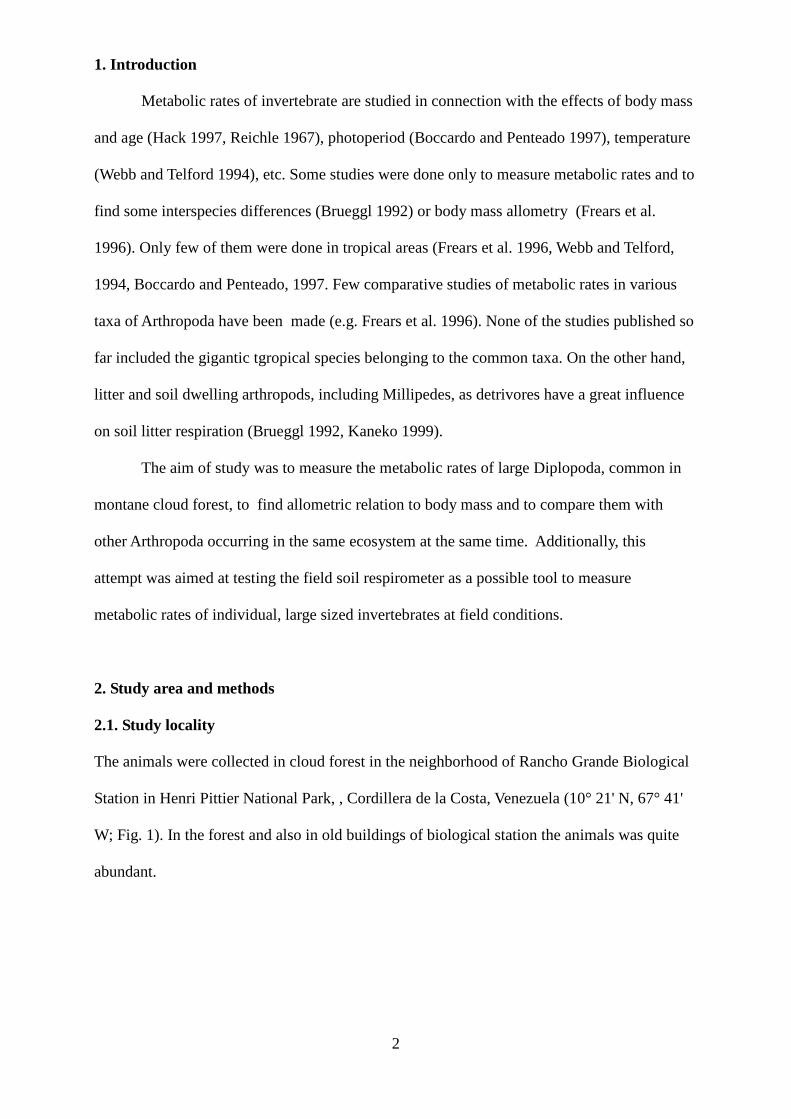
The regressions were significant with R2 value varying between 0.6534 and 0.9934,

most often R2 > 0.9 (Fig. 6).

6

Fig.6. Example of a single measurement record illustrating the linear increase of CO2

concentration [ppm] in the chamber during measurement The slope coefficient of the

regression represents metabolic rate of the animal. The intercept, as expected, did not differ

from the CO₂ concentration in ambient atmosphere (ppm).

3.2. Average respiration rates

Average values of respiration for all taxa studied are given in Table 1.

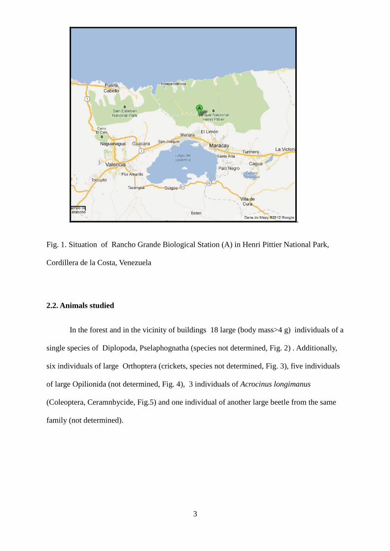
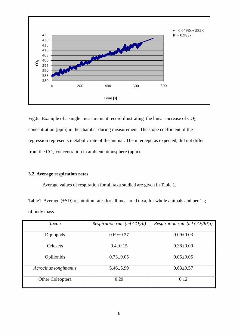
Table1. Average (±SD) respiration rates for all measured taxa, for whole animals and per 1 g

of body mass.

Taxon Respiration rate (ml CO2/h) Respiration rate (ml CO2/h*g)

Diplopods 0.69±0.27 0.09±0.03

Crickets 0.4±0.15 0.38±0.09

Opilionids 0.73±0.05 0.05±0.05

Acrocinus longimanus 5.46±5.99 0.63±0.57

Other Coleoptera 0.29 0.12

7

3.3. Relation between body mass and respiration rate

For Diplopoda the relation body mass vs. respiration rate was significant (R2 =

0.5824) and regression equation on log transformed data was:

y = -0.7625 + 0.6352 x; r = 0.7632; p=0.0002 (Fig. 7),

where x – log(body mass, g), y – log(metabolic rate, mlCO2/h), or:

Y = 0.1728 X0.6352,

where X – body mass (g), Y – metabolic rate (mlCO2/h).

The respiration rates of each individual was averaged also the body mass. Outliers

were removed from analysis. On the averaged data the allometric regression was made.

Fig.7. Allometric relation between body mass and respiration in Diplopoda

4. Discussion

4.1. Validation of the results

The use of soil respirometry apparatus to measure metabolic rates of individual proven

to be quite satisfactory. The exact linearity and narrow confidence limits of regressions of

8

CO2 concentration increase in time, with intercept not differing from expected concentration,

allow for a reliable estimate of the respiration rates. Less satisfactory was the measuring

protocol. The field conditions did not allow for precise control of ambient temperature nor to

record the animals’ behavior, therefore the effects of the locomotor activity could not be

taken into account.

4.2. Allometry of metabolism in Diplopoda

Value of exponent in allometric regression equation (0.6352) departs from value 0.75

reported as a general approximation for large poikiloterm and homeoterms (Reichle, 1967),

and also from the value 0.73 estimated for metabolism of various arthropods taxa, including

Myriapoda (Frears et al., 1996). The respiration rate of large Diplopoda differs from that of

small ones studied in Alps (Brueggl 1992).

4.3. Comparision between various invertebrate taxa

The paucity of does not allow to calculate allometric regression and uniformly

compare all taxa studied. However, if plotted on a graph (Fig. 8) our results show that large

Diplopoda have lower respiration rates than the other taxa studied. Among the arthropods

investigated here, the highest metabolic rates (at their body size) achieved cerambycid

beetles, particularly the Harlequin beetle (A.l), whereas the crickets and Opilionidas

demonstrated relatively low metabolic rates.

Other studies showed that centipeds have lower respiration rate than other

poikiloterms (Webb and Telford, 1994), however yet another comparision showed no

statistically significant differences of respiration rate between millipedes, spiders, ants and

beetles. (Frears et al., 1996).

Because the chamber used here was not transparent, it was not possible to observe the

activity of studied animals during measurement. Only in case of Harlequin beetle it can be

heard that animal was actively moving inside the chamber and this is the case of the

9

extremely high metabolic rate in one specimen (Fig. 8).

Fig. 8. Comparison between metabolic rates in various taxa of arthropods studied, with regard

to body mass.

Conclusions

(1). Diplopoda have lower respiration rate than cerambycid beetles and cricket studied.

(2). The exponent of allometric function among large Diplopoda is smaller than

literature value for small Diplopoda.

(3) The method of measurement with closed chamber and diffusion CO2 analyser

proved to be reliable and useful in harsh field conditions, when applied animals (in case of

Diplopoda) weighing more than 3 g or Orthoptera more than 1g. In further research

transparent chamber should be used to observe the activity of animals.

Acknowledments

The authors want to thank Prof. dr hab. January Weiner for help during the field work

and preparing the report.

10

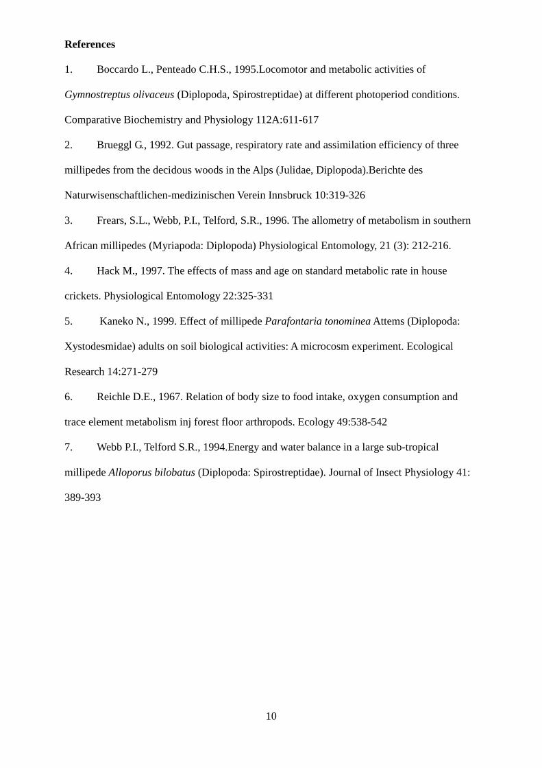
References

1. Boccardo L., Penteado C.H.S., 1995.Locomotor and metabolic activities of

Gymnostreptus olivaceus (Diplopoda, Spirostreptidae) at different photoperiod conditions.

Comparative Biochemistry and Physiology 112A:611-617

2. Brueggl G., 1992. Gut passage, respiratory rate and assimilation efficiency of three

millipedes from the decidous woods in the Alps (Julidae, Diplopoda).Berichte des

Naturwisenschaftlichen-medizinischen Verein Innsbruck 10:319-326

3. Frears, S.L., Webb, P.I., Telford, S.R., 1996. The allometry of metabolism in southern

African millipedes (Myriapoda: Diplopoda) Physiological Entomology, 21 (3): 212-216.

4. Hack M., 1997. The effects of mass and age on standard metabolic rate in house

crickets. Physiological Entomology 22:325-331

5. Kaneko N., 1999. Effect of millipede Parafontaria tonominea Attems (Diplopoda:

Xystodesmidae) adults on soil biological activities: A microcosm experiment. Ecological

Research 14:271-279

6. Reichle D.E., 1967. Relation of body size to food intake, oxygen consumption and

trace element metabolism inj forest floor arthropods. Ecology 49:538-542

7. Webb P.I., Telford S.R., 1994.Energy and water balance in a large sub-tropical

millipede Alloporus bilobatus (Diplopoda: Spirostreptidae). Journal of Insect Physiology 41:

389-393

1

Soil respiration in mountain forests of the Henri Pittier National Park. Małgorzata Boho1, Melanie Renard2 1Faculty of Biology and Earth Sciences. Jagiellonian University: biology and geology 2Faculty of Biology and Earth Sciences. Jagiellonian University: Project ERASMUS at the Institute of Zoology Report submitted in partial fulfillment of the requirements for the course “Tropical ecology – field course” (WBNZ-850), at the Faculty of Biology and Earth Sciences, Jagiellonian University. Abstract: Soil respiration was measured in four different locations at the elevations of 760, 1174, 1201, 1514 m a.s.l., representing various types of tropical mountain forests and cloud forests near Rancho Grande, in the Henri Pittier National Park, Venezuela. Respiration rates differed between sites, ranging from 0.402 to 0.658 g CO2 m-2h-1, with the maximum at the lowest locality. Repeated measurements at one site demonstrated high spatial and temporal variation of respiration rates. Key words: soil respiration, tropical cloud forests Introduction

The CO₂ emission from the soil is an important component of carbon fluxes in forest ecosystems; a detailed knowledge of soil respiration is necessary to cope with environmental and economic issues of today. Soil respiration is a sum of o two processes: root respiration (autotrophic respiration) and litter decomposition by soil organisms (heterotrophic respiration). Numerous studies have shown that many factors affect soil respiration. In temperate regions, temperature is the main factor of variability of CO₂ emission from the soil (Fang, 1998). In the tropics, due to small temperature amplitudes at the ground level, this factor has little influence, but soil moisture and topography are important factors in soil respiration (Pargade, 2000). Some factors act specifically on the autotrophic component of the phenomenon as density and size of the roots (Janssens, 1998). The tropical forests are relatively poorly studied in that respect although they an important sink of carbon.

The aim of this study was make a preliminary investigation in situ in order to get some insight into the patterns of variation of soil respiration in tropical montane forests in connection with the planned more advanced research project in collaboration between the Jagiellonian University and the Central University of Venezuela. It included a preliminary selection of study sites and testing the field equipment. Materials and Methods

The study was conducted in the National Park Henry Pittier, Cordillera de la Costa (near Maracay, Aragua State, Venezuela) in the area surrounding the biological station Rancho Grande (coordinates : N10°20’58,1” W67°41’03,3”). The station is situated at 1180 m a.s.l and is surrounded by four different vegetation types (semi-deciduous forest, tropical cloud forest transitional, cloud forest sensu stricto and high elevation tropical cloud forest; Huber 1986). The climate is defined as a mountain wet tropical one. The annual temperatures fluctuate around 20°C the whole year with low

2

amplitude (averages : 18.4°C in January, 21°C in July). The annul precipitations ranges from 1650 to 1850 mm, depending on local elevation and exposition (Huber 1986).

Four study sites were established: (1) “La Toma “ – close to the station, coordinates

N10˚20’55”, W67˚40’55” , elevation 1201 m a.s.l., “Cumbre” (Peak of the Cumbre de Rancho Grande; N10˚21’20”, W67˚41’20”, 1514 m a.s.l.), “Portachuelo” (close to Portachuelo Pass; N10˚20’47”, W67˚41’18”, 1174 m a.s.l.) and “Guamita” (Guamita valley; N10˚20’20”, W67˚39’18”, 760 m a.s.l.). The sites La Toma and Portachuelo are located at approximately the same elevation, but differ in exposition: Portachuelo is exposed to N – NE, while La Toma to S – SW, therefore, they differ in vegetation type. Portachuelo may be regarded a typical cloud forest, while La Toma area was classified by Huber (1986) to cloud forest transitional. “Cumbre” represent high elevation cloud forest, and Guamita is a semi-evergreen forest, with distinctly different vegetation.

At La Toma and Portachuelo linear transects were marked out with 20 and 22 measuring stations at 1 m distance. Due to logistic problems a similar transect at Guamita included only 7 measuring stations. At the hilltop of Cumbre, 17 measuring points were randomly selected within appr. 50 m radius from the coordinates indicated, with different slopes and exposition.

At each study site except La Toma respiration neasurements were done only once (Cumbre: July 11, Portachuelo: July 10, Guamita: July 12, 2012); at La Toma measurements were repeated 4 times (July 6, 8, 10 and 14), with measuring chamber placed each time exactly in the same spot.

To measure soil respiration, we used a plastic chamber of the volume of 3.2 l, covering soil surface of 240.2 cm2 and CO2 concentration sensor Vaisala GMP343, linked to a computer (Fig.1), recording CO2 concentration in the chamber at 1 sec intervals. Measurements lasted usually for 2-3 min. To each record a linear regression was fitted, the slope coefficient of which represented the rate of CO2 concentration increase, which subsequently was recalculated into g CO2 × m-2 × h-1 using appropriate data on chamber dimensions.

Soil temperature was measured at the depth 5 cm using digital thermometer GTH 175/PT (Greisinger electronic) with accuracy of 0.1˚C.

Fig. 1 Soil respirometer: chamber with the Vaisala GMP 343 CO2 sensor, interface, and computer.

3

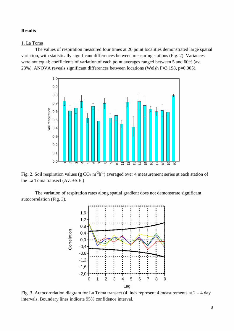
Results 1. La Toma

The values of respiration measured four times at 20 point localities demonstrated large spatial variation, with statistically significant differences between measuring stations (Fig. 2). Variances were not equal; coefficients of variation of each point averages ranged between 5 and 60% (av. 23%). ANOVA reveals significant differences between locations (Welsh F=3.198, p=0.005).

Fig. 2. Soil respiration values (g CO2 m-2h-1) averaged over 4 measurement series at each station of the La Toma transect (Av. ±S.E.) The variation of respiration rates along spatial gradient does not demonstrate significant autocorrelation (Fig. 3). Fig. 3. Autocorrelation diagram for La Toma transect (4 lines represent 4 measurements at 2 – 4 day intervals. Boundary lines indicate 95% confidence interval.

1 2 3 4 5 6 7 8 9 10 11 12 13 14 15 16 17 18 19 20

0,0

0,1

0,2

0,3

0,4

0,5

0,6

0,7

0,8

0,9

1,0

Soi

l res

pira

tion

0 1 2 3 4 5 6 7 8 9Lag

-2,0-1,6-1,2-0,8-0,40,00,40,81,21,6

Cor

rela

tion

4

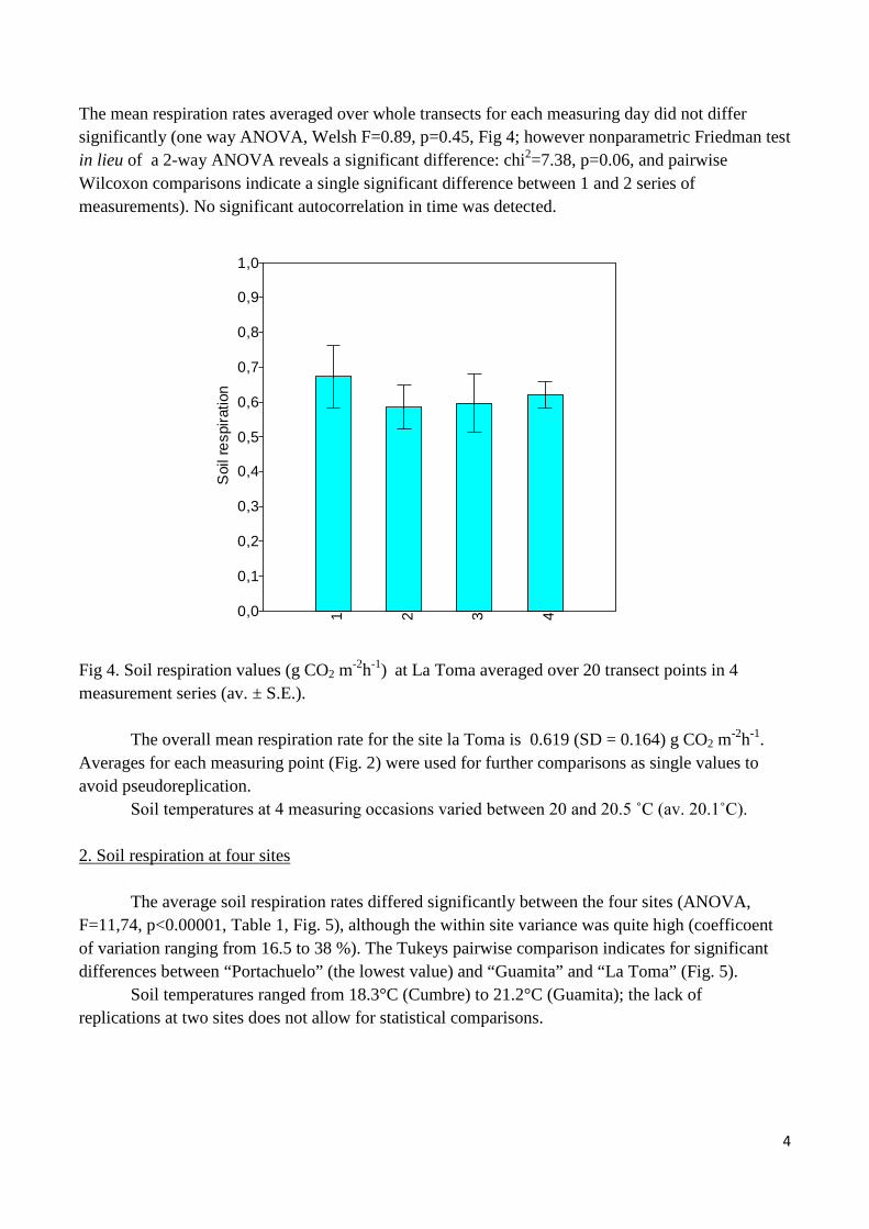
The mean respiration rates averaged over whole transects for each measuring day did not differ significantly (one way ANOVA, Welsh F=0.89, p=0.45, Fig 4; however nonparametric Friedman test in lieu of a 2-way ANOVA reveals a significant difference: chi2=7.38, p=0.06, and pairwise Wilcoxon comparisons indicate a single significant difference between 1 and 2 series of measurements). No significant autocorrelation in time was detected. Fig 4. Soil respiration values (g CO2 m-2h-1) at La Toma averaged over 20 transect points in 4 measurement series (av. ± S.E.). The overall mean respiration rate for the site la Toma is 0.619 (SD = 0.164) g CO2 m-2h-1. Averages for each measuring point (Fig. 2) were used for further comparisons as single values to avoid pseudoreplication.

Soil temperatures at 4 measuring occasions varied between 20 and 20.5 ˚C (av. 20.1˚C). 2. Soil respiration at four sites The average soil respiration rates differed significantly between the four sites (ANOVA, F=11,74, p<0.00001, Table 1, Fig. 5), although the within site variance was quite high (coefficoent of variation ranging from 16.5 to 38 %). The Tukeys pairwise comparison indicates for significant differences between “Portachuelo” (the lowest value) and “Guamita” and “La Toma” (Fig. 5). Soil temperatures ranged from 18.3°C (Cumbre) to 21.2°C (Guamita); the lack of replications at two sites does not allow for statistical comparisons.

1 2 3 40,0

0,1

0,2

0,3

0,4

0,5

0,6

0,7

0,8

0,9

1,0

Soi

l res

pira

tion

5

Table 1. Average values of soil respiration at four sites studied.

SITE CUMBRE GUAMITA PORTACHUELO LaTOMA Altitude [m] 1514 760 1174 1201

Soil temperature [°C] 18.3 21.2 19.5 20.1

S.D. 0.76 0.25 Respiration [g CO2 m-2h-1]

n 16 7 22 20 Mean 0.524 0.658 0.402 0.619 S.D. 0.134 0.153 0.152 0.102 S.E. 0.033 0.058 0.033 0.023 Min 0.349 0.442 0.153 0.416 Max 0.757 0.865 0.722 0.794

Fig. 5. Soil respiration (g CO2 m-2h-1); site averages ± 95% confidence intervals. Letters above the bars indicate homogenous groups.

CU

MBR

E

GU

AMIT

A

RTA

CH

UE

LaTO

MA0,0

0,1

0,2

0,3

0,4

0,5

0,6

0,7

0,8

0,9

1,0

Soi

l res

pira

tion

abc ac b a

6

Discussion The soil temperature decreases linearly with elevation a.s.l. as it can be expected (Fig. 6). The soil temperature elevation gradient is 0.38 deg per 100 m, i.e. less than it usually assumed for air at maximum humidity (0.6 deg/100m). However, the soil respiration rates do not fully with temperature pattern (Fig. 7), as it could have been predicted from the usual exponential dependence of soil respiration rates on temperature (Luo and Zhou, 2006). The lowest soil respiration was recorded at Portachuelo, the highest at Guamita (Table 1, Fig. 7). Fig 6. Soil temperature at different elevations a.s.l. Fig. 7. Soil respiration as related to soil temperature (exponential regression fitted).

y = 0,0712e0,1026x R² = 0,3165

0,35

0,4

0,45

0,5

0,55

0,6

0,65

0,7

18 18,5 19 19,5 20 20,5 21 21,5

Soil

resp

iratio

n [g

CO

2 m-2

g-1 ]

Soil temperature [°C]

7

The exponential regression fitted to these data yields the exponent 0.1026, which can be translated in a Q10 value of 2.79. When excluding the outlying data point for Portachuelo, the exponential regression fits almost exactly to the remaining three points (R2 = 0.986), with the exponent and Q10 values equal 0.0795 and 2.21, respectively. These figures are close to those reported for soil respiration data in various climates (Luo and Zhou 2006). Respiration rates measured in montane and cloud forests of cordillera de la Costa at one point of annual season appear relatively high, as compared to the generalized data published so far for moist tropical forests. E.g., Luo and Zhou 2006 give the value of 1260 g CO2 m-2year-1 (i.e. 0.14 g CO2 m-2h-1) for tropical moist forests. A study performed during one season only (1985/86), at Loma de Hierro (N10˚8’20” , W67˚8’30”, 1350 m a.s.l., about 70 km east from Rancho Grande), using soil respiration estimation by chemical absorption, revealed that the soil respiration demonstrated high variation (av. 0.369 ± 0.180 g CO2 m-2 h-1); a few others single estimates of soil respiration from the same region were similarly varied (La Cumbre de Choroni: 0.346 g CO2 m-2 h-1, Rancho Grande: 0.195 g CO2 m-2 h-1; Medina and Zelwer 1972; after Monedero and Gonzalez 1995), but no attempt was made to explain the sources of this variation. Our measurement at La Toma site, with four replication, also demonstrate high variation, both in time and in space. Although some pattern of differences between transect points is significant, indicating for existing repeatability of soil respiration rates measured at the same spot over time, it is much less distinct and less stable than analogous patterns in temperate forests in Poland (Matkowska et al., unpubl.). Conclusions 1. Soil temperature decreases with elevation. 2. Soil respiration differs between the sites located at various elevations, with the highest rate at the lowest and the warmest site. 3. Respiration values are close to previously reported for adjacent areas and similar forest types. 4. Soil respiration dependence on temperature seems to conform with general predictions (Q10 = 2.2) but more data with longer temperature gradients and covering the whole year are needed. 5. The closed soil respirometry system based on Vaisala GMP 343 CO₂ probe, with a closed chamber, and portable computer proved to be useful and dependable in field conditions.

8

Literature Fang C., Moncrieff J. B., Gholz H. L., Clark K. L. 1998: Soil CO2 efflux and its spatial variation in a Florida slash pine plantation. Plant and soil. 205 : 135-146. Huber O. (Ed.), 1986: La Selva Nublada de Rancho Grande, Parque National „Henri Pittier”: El Ambiente Fisico, Ecologia Vegetal y Anatomia Vegetal. Fondo Editorial Acta Científica Venezolana. Seguros Anauca C.A., Caracas. Janssens I. A. ; Barigah S. T. ; Ceulemans R.. 1998: Soil CO2 efflux in different tropical vegetation types in French Guiana. Ann. For. Sciences. 55 : 671-680. Luo Y., Zhou X., 2006. Soil respiration and the environment. Elsevier, Amsterdam. 316 pp. Medina E., Zelwer M., 1972. Soil respiration in tropical plant communities. In. P.M. Golley, F.B. Golley (eds.) Tropical ecology with an emphasis on organic production. University of Georgia, Athens. Monedera C., González V., 1995. Producción de hojarasca y decomposición en una selva nublada del ramal interior de la Cordillera de la Costa, Venezuela (Litterfall and decomposition in a cloud forest of the Cordillera de la Costa, Venezuela). Ecotropics 8 (1-2): 1-14. Pargade J.. 2000: Analyses des variations spatio-temporelles du flux de CO2 d’un sol forestier mesuré par la méthode dynamique. DEA de Biologie Forestière. Université H. Poincaré. Nancy. INRA Bordeaux. Zimmermann M.. Bird M.I.. 2012 Temperature sensitivity of tropical forest soil respiration increase along an altitudinal gradient with ongoing decomposition. Geoderma 187-188: 8-15

1

Daily activity of leaf cutting ants Acromyrmex coronatus.

Katarzyna Jabłońska

Wiktoria Kowalińska

Faculty of Chemistry, Jagiellonian University: Environmental protection

Report submitted in partial fulfillment of the requirements for the course “Tropical ecology – field course” (WBNZ-850), at the Faculty of Biology and Earth Sciences, Jagiellonian University.

Abstract

Daily activity patterns, average velocity and the amount of biomass carried by ants

Acromyrmex coronatus were studied in montane cloud forest in Henri Pitter National

Park, Venezuela. The most intense activity was recorded in the morning and in the middle

of the day on the 24 hours active path and before midnight on the path used only in the

night. The velocity of ants averaged to 0.03 m/sec, and varied with direction of moving,

maximum of 0.059 m/sec on vertical path down – hardly with a load. The wet biomass

delivered to the nest was estimated at 3.26 kg/day (dry mass content 23.81%).

Key words: Acromyrmex coronatus, biomass, activity patterns

1. Introduction

Attini of the genus Acromyrmex comprise twenty six leaf cutting ants species, described

from throughout the Neotropics (Hölldobler and Wilson, 1990). They are endemic to

South and Central America and southern parts of North America. They cut fresh

vegetation, which is processed and used as a substrate for their fungus symbiont

(Klingenberg et al., 2007). Leaf cutting ants may cause deforestation and strongly affect

forest succession on abandoned land (Moutinho et al., 2003). Genus Acromyrmex is the

most serious agricultural pest of tropical and subtropical America, causing enormous

economic damage to the neotropic agriculture industry (cf. Cherrett 1986, after Wirth R.,

Herz H., Beyschlag W., Holldobler B., 2007). The aim of this study was to monitor the 24

hours activity of ants carrying plant material to determine their average velocity, and to

estimate the amount of plant biomass transported into the nest.

2

2. Materials and methods

2.1. Study area

The project was realized in the field station “Rancho Grande” belonging to the Faculty of

Agronomy, Central University of Venezuela, Maracay. Rancho Grande is situated in

mountain cloud forest in the Henri Pittier National Park of Aragua, in north central

Venezuela (10° 21' N. Lat., 67° 41' W. Long). The study was done in July 2012, during a

wet season.

The nest of Acromyrmex is located closely to the walls of Rancho Grande field station.

We found two active paths. One of them was active 24 hours and ran upon the wall, 9

meters up, to the birds’ feeder. On this path ants used unusual type of food – mainly

watermelon, banana and mango, and occasionally the leaves and flowers of Tabebuia

chrysantha, a tree growing nearly. The second path was used only during night and ran on

the trunk of Tabebuia tree, where the ants carried almost exclusively Tabebuia leaves as a

load.

2.2. Data collection and analysis

2.2.1. Activity pattern

To determine 24 hours activity of Acromyrmex ants, we have recorded ants on their path

during 10 minutes using a movie camera. This allowed to count ants moving in both

directions in the same time period. The ants were counted on two paths: on the wall and

on the tree trunk. To estimate the time of opening and closing the night path we checked

the time of first ascending and last descending and repeated this observation three times.

2.2.2. Average velocity

The velocity of ants in different places was measured by using the timer and measuring

tape. We made 10 measurements of velocity of ants on the 1 meter distance, for every

type of the path: on the tree (in both directions- up and down), on the wall (vertical path-

both directions, horizontal path). To compare the velocities of ants measured per one

meter distance and on the long path (on the wall), we measured the length of the path

from birds feeder to the nest (15.9 m). Then we used nail polish to mark the ants at the

3

starting point and measured the time of the arrival of the marked individuals at the end of

the way. We included the information about type of path, direction of moving

(horizontal/vertical) and load during measurement velocity on the long day path.

2.2.3. Biomass carried

To determine the weight of wet and dry biomass carried we collected 10 samples of 10

pieces of leaves Tabebuia from the path on the tree. We weighed all wet leaves together

on the electronic portable balance (Voltcraft PS500X with the accuracy of 0.01 g). We

dried the biomass by careful heating and using silica gel to achieve dry mass weight. The

calculated weight of single piece of leaf, multiplicated by the number of ants per time

period, yielded the quantity of biomass delivered in kilograms per day.

We used “Statistica” and Microsoft Excel programs for statistical analyses.

3. Results

3.1 Activity patterns

The highest activity of ants on the both paths, was observed in the night, before midnight

(Fig. 1.). At 11 p.m., we counted 536 ants per 10 minutes, and it was the highest number

of ants in this period. After midnight a significant decline was observed (Fig. 1.). At 6

a.m., only a very small number of individuals was noticed.

On the path on the wall, the quantity of ants was the highest in the morning and in the

middle of the day. In the night, their activity was stable, but not high. (Fig. 2.).

During night path observation, ants started to be active about 18:00 p.m. (average from

three measurements) and they stopped their activity about 05:30 a.m. The highest activity

of ants on tree was observed before midnight (Fig. 3.).

3.2 Average velocity

The highest velocity of ants, was observed down the wall, despite loading. The lowest

velocity had ants ascending. The results from the path on the tree and on the wall did not

differ significantly (Fig. 4.)

4

Statistical analyses show significant differences (p<0.005) for directions of moving.

Average velocity of ants moving on the horizontal path on the wall was statistically

different from the velocity of ants ascending and descending, on the both paths – on

the tree and on the wall (Tab. 1). Type of path was statistically different only for the

path on the tree, for the ants moving horizontally and ascending on the wall (Tab. 1.).

Comparing average velocity on short distance to long distance shows that average

velocity on long distance was lower than on the short, but that there is no statistically

significant difference between the two speeds.

Average velocity on short distance (1 meter) amounts 0.03 +/- 0.005 m/s.

Average velocity on long distance (15.9 meters) amounts 0.025 +/- 0.005 m/s.

3.3. Biomass carried

Wet mass of 100 pieces of leaves was 2.52 g, thus one piece was on average 0.0252 g.

The dry mass of 100 pieces of leaves was 0.60 g., what gives the mass of 0.006 g per

piece.

4. Discussion

4.1. Activity patterns

Location of ants nest (close to the station) made it possible to measure 24 hr activity

pattern of ants. We have accurate data from the whole day and night. The most intense

activity of Acromyrmex sp., recorded in the morning and in the middle of the day on

the path on the wall is probably caused by unusual feeding system (feeding by people,

mainly fruits). On the tree before midnight a lot of ants were climbing up the tree to

get pieces of Tabebuia’s leaves. During our observation a social behavior was visible.

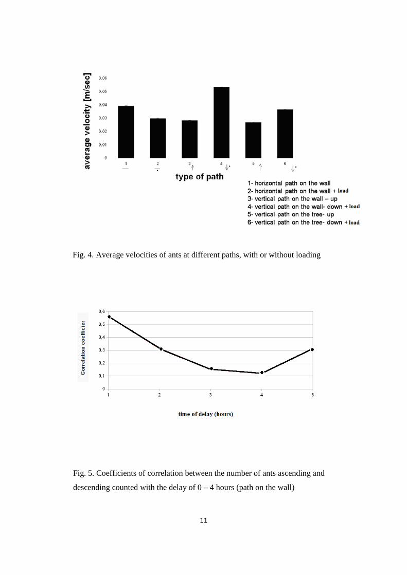
The graph of correlation coefficient between number of ants ascending and descending

with the delay of 0 – 4 hours (path on the wall) shows, that ants on the wall need about

one hour to ascent and descent. Some ants descent after two hours (Fig. 5.) The ants

5

on the tree needed one hour to go up and down, so they require less time than ants on

wall. Probably they have shorter way (Fig. 6).

4.2. Average velocity

Contrary our expectations, loading did not influence the velocity – ants with load or

without it had similar speed (comparison on the same type of path; Fig. 4, Tab. 1). The

velocity depends the most on the direction of moving - vertical or horizontal (Fig. 4,

Tab. 1). The highest velocity occurs down the. The small statistical difference occurs

between the speed on the different type of the path (Fig. 4, Tab. 1.). The comparison

short and long distance velocity show that velocity from whole path (from feeder to

the nest) is lower, but not statistically different. This may be caused by the nail polish

used to mark the ants which coul affect the behavior.

4.3. Biomass carried

Ants deliver 3.26 kg of biomass/day, dry mass constitute 23.81% of biomass, thus per

1 day ants are delivering 0.78 kg of dry mass. Recalculated average mass of the load

for the whole year (assuming identical activity in all seasons and that there are no

other paths) it gives about 1189.9 kg of wet biomass or 284.7 kg of dry mass of plant

material. On the base of previous research (Soszka and Zieliński, 2010), we assume

that wet biomass of fruits from birds’ feeder, amount 31 kg/year, thus gives 1220.9

kg/year of wet biomass carrying from the both paths. They found only one path (24

hours active path on the wall with unusual type of foods) and they did not measured

wet biomass from path on the tree. Comparing the result from previous year on Atta

sp. (Grzech and Grucza, 2008), the biomass of leaves carried into the nest by the ants

Atta cephalotes), we can see similar amount of wet biomass - 1182 kg/year and 390

kg/year of dry mass of plant, delivered to the nest of Atta cephalotes. Differences

could be caused by the methods - they were observing ants only in the daytime, and no

data are available about the possible night activity of Atta. We can suppose that if the

study would be 24h the results could be different. In our studies we tried to estimate

influence on vegetation by leaf cutting ants, thinking mainly about direct effects

caused by defoliation. Colony of Acromyrmex coronatus ants can cause serious

damage, due to significant amount of using biomass. But ants may have also indirect

impact on vegetation. Injuries caused to leaves open the possibility of infection by

6

fungi, bacteria and viruses. On the other hand, indirect effects include soil nutrient

enrichment from nest refuse dumps and transferring nutrient to upper soil layers

(Weber 1972).

Acknowledgments

We would like to thank Professor January Weiner from Jagiellonian University for his

invaluable knowledge and professional advices during our project. Special thanks to

the IVIC staff for support and guidance during this course. We wish to thank dr hab.

Krzysztof Wiąckowski for sharing his experience and guidance.

5. References

Grzech U., Grucza K. (2008). The biomass of leaves carried into the nest by the ants

Atta cephalotes . Raports from Tropical Ecology Field Course WBNZ-850, 2008:

http://wko.uj.edu.pl/tropiki/Raporty/2008_Reports.pdfww.e

Hőlldobler B., Wilson E. O., (1990). The Ants. Harvard University Press, Cambridge.

Klingenberg C., Brandao C. R. F., Engels W., (2007). Primitive nest architecture and

small monogynous colonies in basal Attini inhabiting sandy beaches of southern

Brazil. Studies on Neotropical Fauna and Environment, 42: 121-126.

Laskowski R., Pyrcz T., Weiner J. (2012) Guide for common plants and Animals of

Venezuela; Institute of Eniviromental Sciences, Jagiellonian University, Kraków.

Mountinho P., Nepstad D.C., Davidson E.A. (2003). Influence of leaf – cutting ant

nests on secondary forest growth and soil properties in Amazonia, Ecology, 84 : 1265-

1276.

Soszka A., Piotr Zieliński P. (2010) Foraged biomass of the Leaf-Cutter Ants Atta

Cephalotes and Acromyrmex coronatus: findings from research undertaken at the field

station of Rancho Grande in Henri Pittier National Park, Venezuela. Raports from

Tropical Ecology Field Course WBNZ-850, 2010:

http://wko.uj.edu.pl/tropiki/Raporty/2010_Reports.pdfww.e

7

Wirth R., Herz H., Beyschlag W., Holldobler B. (2007) Herbivory rate of leaf-cutting

ants in a tropical moist forest in Panama at the population and ecosystem scales.

Biotropica, 39: 482-488.

Weber N. A., (1972). Gardening ants. The attines. American Philosophical Society,

Philadelphia. 146 pp.

8

Appendix

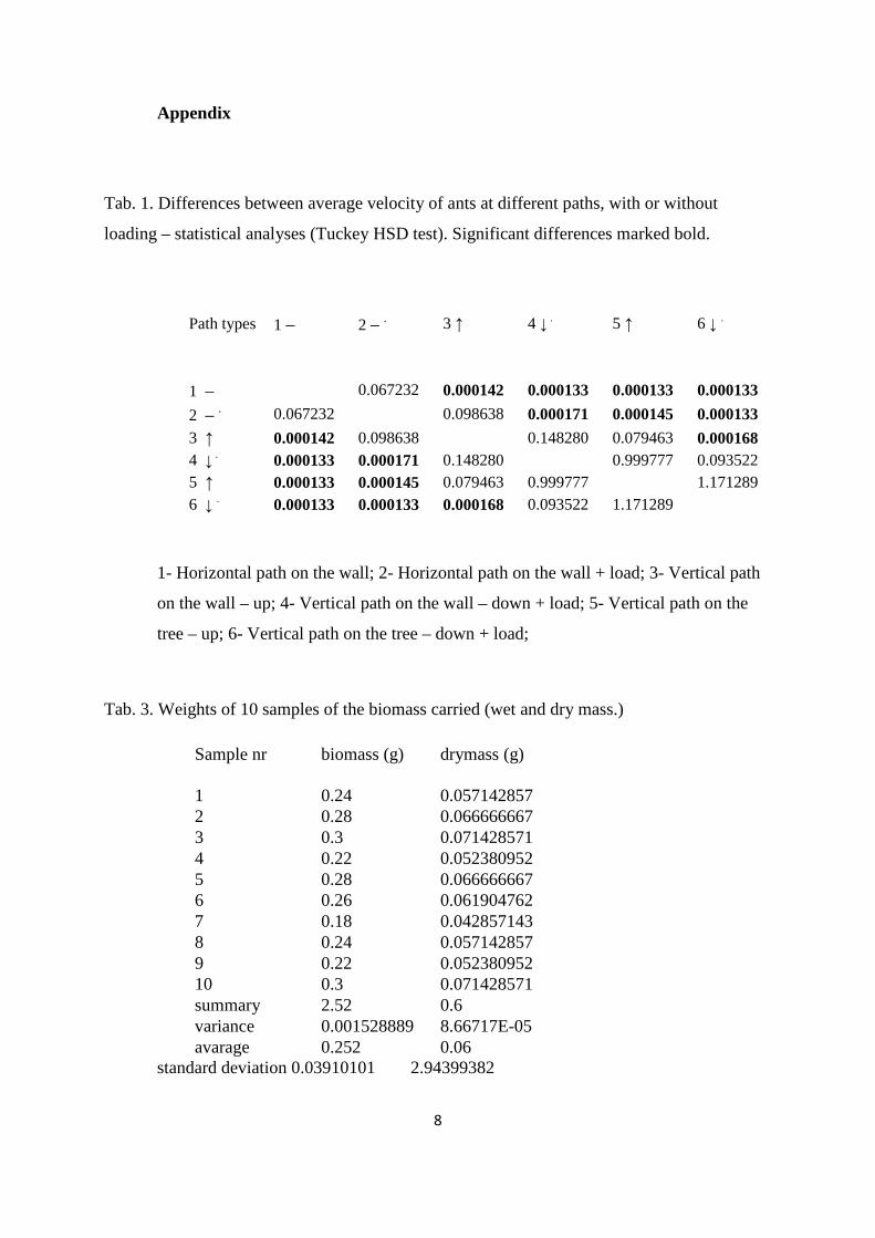
Tab. 1. Differences between average velocity of ants at different paths, with or without

loading – statistical analyses (Tuckey HSD test). Significant differences marked bold.

Path types 1 –

2 – .

3 ↑

4 ↓ .

5 ↑

6 ↓ .

1 – 0.067232 0.000142 0.000133 0.000133 0.000133 2 – . 0.067232 0.098638 0.000171 0.000145 0.000133 3 ↑ 0.000142 0.098638 0.148280 0.079463 0.000168 4 ↓ . 0.000133 0.000171 0.148280 0.999777 0.093522 5 ↑ 0.000133 0.000145 0.079463 0.999777 1.171289 6 ↓ . 0.000133 0.000133 0.000168 0.093522 1.171289

1- Horizontal path on the wall; 2- Horizontal path on the wall + load; 3- Vertical path

on the wall – up; 4- Vertical path on the wall – down + load; 5- Vertical path on the

tree – up; 6- Vertical path on the tree – down + load;

Tab. 3. Weights of 10 samples of the biomass carried (wet and dry mass.)

Sample nr

biomass (g)

drymass (g)

1 0.24 0.057142857 2 0.28 0.066666667 3 0.3 0.071428571 4 0.22 0.052380952 5 0.28 0.066666667 6 0.26 0.061904762 7 0.18 0.042857143 8 0.24 0.057142857 9 0.22 0.052380952 10 0.3 0.071428571 summary 2.52 0.6 variance 0.001528889 8.66717E-05 avarage 0.252 0.06

standard deviation 0.03910101 2.94399382

9

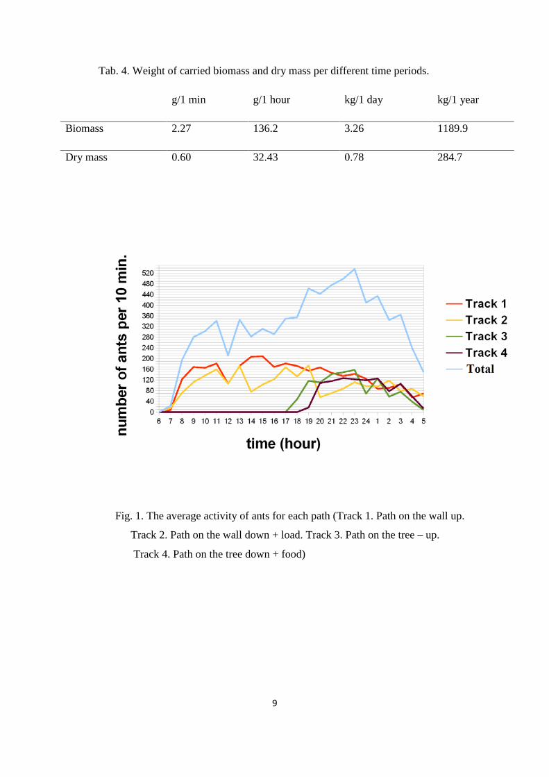
Tab. 4. Weight of carried biomass and dry mass per different time periods.

g/1 min g/1 hour kg/1 day kg/1 year

Biomass 2.27 136.2 3.26 1189.9

Dry mass 0.60 32.43 0.78 284.7

Fig. 1. The average activity of ants for each path (Track 1. Path on the wall up.

Track 2. Path on the wall down + load. Track 3. Path on the tree – up.

Track 4. Path on the tree down + food)

10

Fig. 2. Average activity of ants on the wall- 24h observation

(Track 1. Path on the wall - up. Track 2. Path on the wall - down)

Fig. 3. Average activity of ants on the tree - night observation

(Track 1. Path on the tree - up. Track 2. Path on the tree - down)

11

Fig. 4. Average velocities of ants at different paths, with or without loading

Fig. 5. Coefficients of correlation between the number of ants ascending and

descending counted with the delay of 0 – 4 hours (path on the wall)

12

Fig. 6. Coefficients of correlation between the number of ants ascending and

descending counted with the delay of 0 – 4 hours (path on the tree)

1

Light regime preferences in selected plants of neotropical cloud forest.

Karol Szurdak1. Sylwia Buczek2

1Faculty of Biology and Earth Sciences. Jagiellonian University: biology and geology 2Faculty of Biology and Earth Sciences. Jagiellonian University: biology Report submitted in partial fulfillment of the requirements for the course Tropical ecology – field course (WBNZ-850) at the Faculty of Biology and Earth Sciences. Jagiellonian University. 2012.

Abstract

The observations done at three open sites and three shadow sites in a montane cloud forest

(Cordillera de la Costa. Venezuela) show that the abundance and species composition of epiphyte

communities on trees depend on the amount of light available.

Comparative measurements of the amount of sunlight reaching leaves’ surface of two

species of Heliconia show that H. bihai prefers more sunny places than H. revoluta.

Key words: light regime. epiphytes. Heliconia sp.

Introduction

The tropics are warm because the sun’s radiation falls more directly. However. cloudiness

and higher water vapor content of the air reduce the amount of solar radiation reaching the forest

canopy. As the availability of light can limit plant growth. it is interesting to learn how the

tropical forest plants adapt to light regime [1.2].

Epiphytes are plants which grow above the ground surface. They are not rooted in the soil.

By growing on other plants. the epiphytes can reach positions where there is more light available

or where they can avoid competition for light [3.4.5]. What is important. epiphytes use their host

plants only as platforms [1.3]. Majority plants use solar radiation as source of energy for

photosynthesis. and also to regulate their process of growth and development. Despite their high

local diversity and abundance. epiphytes grow relatively slowly [6]. Slow growth is probably

caused by poor and irregular availability of water and nutrients. The light intensity is another

ecological factor influencing plant growth [6]. On the other hand. high irradiance will lead to

increased temperature which may influence the plant growth due to overheating and desiccation.

2

As the epiphytes do not have direct access to moisture. they reduce their water loss on several

ways. Many epiphytes close their stomata during the day. Orchids contain bulbous stems in

which they store water. Bromeliads form of their leaves a kind of a water container. Some groups

of plants. such as ferns. Bromeliaceae (Fig.1) and Orchidaceae are particularly abundant in

neotropical epiphyte communities [3-5].

Light availability in tropical forests varies at different heights. It looks differently deep in

the forest, on the forest floor, than in the canopy above. Plant of the understory may differ in light

preferences, some grow well in the shade. while most grow best in sunny places and in open

areas. For instance, it has been reported that Heliconia bihai is growing in conditions with full

sun to 40% shade [7] while other species may do well in shadow. Heliconia bihai (Fig.2) and

Heliconia revoluta (Fig.3) are perennial herbs typically growing taller than 1.5 m, characterized

by long. curved inflorescences. and colorful bracts surrounding little flowers, adapted to avian,

especially hummingbird pollination [3.4]. Heliconia’s bihai inflorescences are standing up (Fig.

2),. constituting water tanks protecting their seeds against insects and a source of water for

animals. In contrast, H. revoluta has the inflorescences reversed, hanging down (Fig. 3). The

species are sympatric, but they may differ with habitat preferences.

The goals of this study were: (1) to check if the abundance and species composition of epiphyte

communities depend on light regime, and (2) to estimate the light regime preferences of two

related plants species: H. bihai and H. revoluta differ.

Fig. 1. A group of Bromeliaceae epiphytes. Photo was made in La Toma area.

3

Fig. 2. Heliconia bihai.

Fig. 3. Heliconia revoluta.

4

Materials and methods

The present study was carried out in the northern part of Venezuela in Cordillera de la

Costa, Parque Nacional Henri Pittier. The studies were carried out at the biological field station

Rancho Grande and its closest surroundings: the path called “La Toma” and education pathway

called “Sendero Andrew Field”.

Epiphytes

The research sites (three exposed and three shadowed ones) were selected, marked in the

field and their position was recorded using a GPS. At each of these sites three to six trees with

epiphytes were chosen for detailed scrutiny. Using binoculars, the morphotaxa of epiphytes were

determined. We have taken into account the following morphotaxa: ferns, Araceae,

“Philodendron”, Vriesea plathynema – “big” Bromeliaceae, “small” Bromeliaceae, Rhipsalis sp.,

Epifilum sp., Vanilla sp., Orchidaceae.

Plants of understory

Seven clusters of Heliconia revoluta and seven of Heliconia bihai were selected and

marked in the Sendero Andrew Fields and La Toma. Intensity of light was measured immediately

at the surface of leaves, during two days 9th and 10th of July.

All statistical analyses were performed with Statistica.

Protocol

Alltogether, nine series of measurements of light intensity at selected stations for

epiphytes were done in various times of day. Measurements were made at a distance of 6-10

meters from the observed trees, in one special point at each site. All measurements were done

with luxmeter MS-1300

During the measurements the cloud cover was observed and recorded. using arbitrary

numerical scale of discrete degrees (Tab.1). Since the measurements were done at various

cloudiness, and at various day hours, a standardization of the light intensity was attempted. To

that purpose to each degree of cloudiness we have attached an index of the average reduction of

light intensity (Tab.2), involving also the time of the day when measurements in situ were done.

5

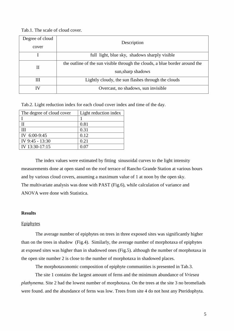
Tab.1. The scale of cloud cover.

Degree of cloud

cover Description

I full light, blue sky, shadows sharply visible

II the outline of the sun visible through the clouds, a blue border around the

sun,sharp shadows

III Lightly cloudy, the sun flashes through the clouds

IV Overcast, no shadows, sun invisible

Tab.2. Light reduction index for each cloud cover index and time of the day.

The degree of cloud cover Light reduction index I 1 II 0.81 III 0.31 IV 6:00-9:45 0.12 IV 9:45 - 13:30 0.21 IV 13:30-17:15 0.07

The index values were estimated by fitting sinusoidal curves to the light intensity

measurements done at open stand on the roof terrace of Rancho Grande Station at various hours

and by various cloud covers, assuming a maximum value of 1 at noon by the open sky.

The multivariate analysis was done with PAST (Fig.6), while calculation of variance and

ANOVA were done with Statistica.

Results

Epiphytes

The average number of epiphytes on trees in three exposed sites was significantly higher

than on the trees in shadow (Fig.4). Similarly, the average number of morphotaxa of epiphytes

at exposed sites was higher than in shadowed ones (Fig.5). although the number of morphotaxa in

the open site number 2 is close to the number of morphotaxa in shadowed places.

The morphotaxonomic composition of epiphyte communities is presented in Tab.3.

The site 1 contains the largest amount of ferns and the minimum abundance of Vriesea

plathynema. Site 2 had the lowest number of morphotaxa. On the trees at the site 3 no bromeliads

were found. and the abundance of ferns was low. Trees from site 4 do not host any Pteridophyta.

6

also they have 2-4 epiphytes from morphotaxon Bromeliaceae. Site 5 contains the largest number

of individuals of Araceae. The trees of site 6 contain the largest number of Bromeliacea (Tab.3).

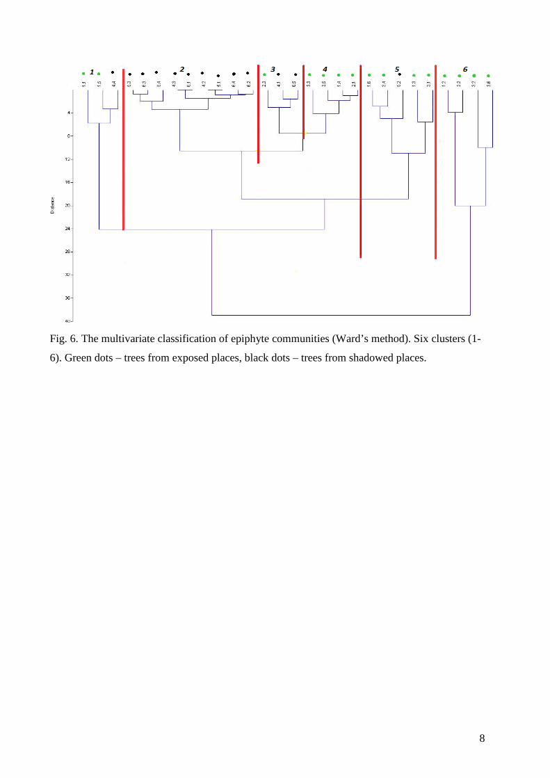
The multivariate cluster analysis classified the epiphyte communities into six clusters

(Fig.6). with a clear segregation of communities in shadowed sites (cluster 2) and those from

exposed localities (clusters 4. 5.6).

The results of light intensity measurements at epiphyte sites did not give a clear pattern.

The average light intensity values (raw) did not differ significantly between the open and the

shadowed sites. The standardization with the model including cloud cover only did reduce the

intra group variance (Tab. 4). but the averages for the sites defined as open and shadowed did

not differ statistically in average light intensities.

Plants of understory

The average light intensities measured at the stands of the both Heliconia species differed

statistically (Fig.7). with H. revoluta preferring darker sites.

7

0

5

10

15

20

25

30

35

40

1 2 3 1 2 3

num

ber o

f epi

phyt

es

11

Fig. 4. The average numbers of epiphytes on trees in three open and three dark sites (green –

open sites. blue – dark sites). Average ± SD.

0

1

2

3

4

5

6

7

8

1 2 3 1 2 3

Fig. 5. The average numbers of morphotaxa of epiphytes at each site (pink – open sites; violet –

dark sites). Average ± SD.

8

Fig. 6. The multivariate classification of epiphyte communities (Ward’s method). Six clusters (1-

6). Green dots – trees from exposed places, black dots – trees from shadowed places.

9

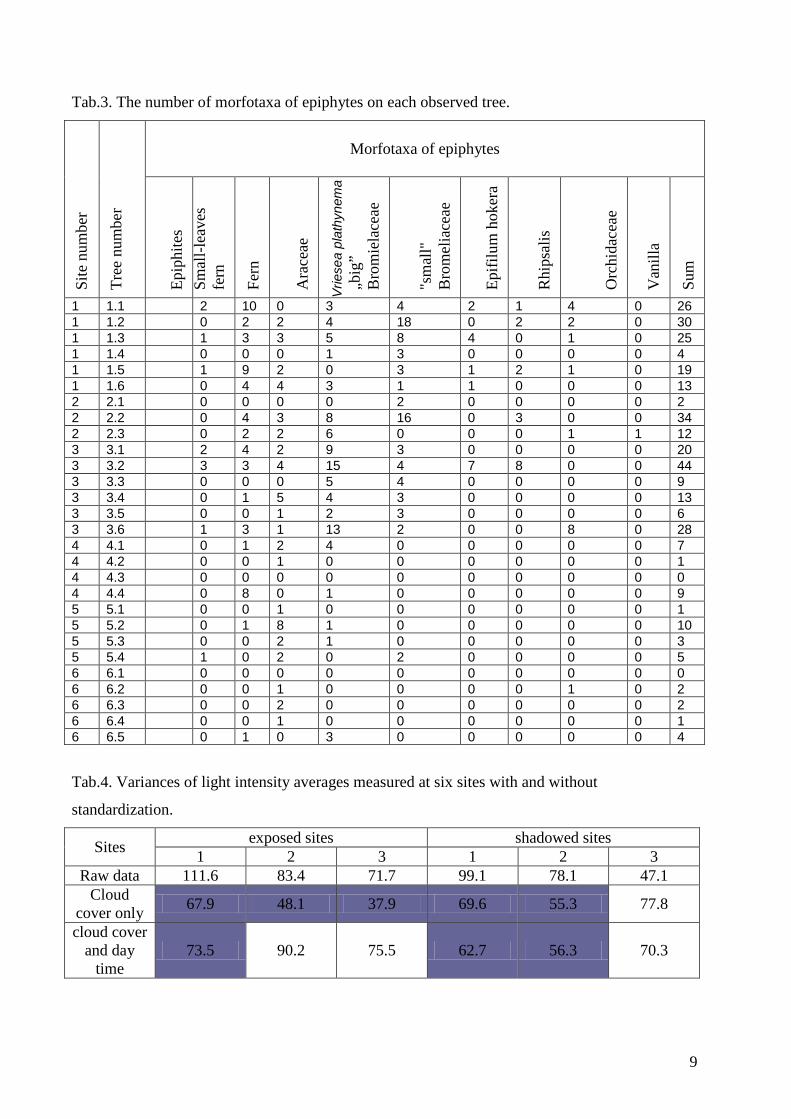
Tab.3. The number of morfotaxa of epiphytes on each observed tree. Si

te n

umbe

r

Tree

num

ber

Morfotaxa of epiphytes Ep

iphi

tes

Smal

l-lea

ves

fern

Fern

Ara

ceae

Vrie

sea

plat

hyne

ma

„big

” B

rom

iela

ceae

"sm

all"

B

rom

elia

ceae

Epifi

lum

hok

era

Rhi

psal

is

Orc

hida

ceae

Van

illa

Sum

1 1.1 2 10 0 3 4 2 1 4 0 26 1 1.2 0 2 2 4 18 0 2 2 0 30 1 1.3 1 3 3 5 8 4 0 1 0 25 1 1.4 0 0 0 1 3 0 0 0 0 4 1 1.5 1 9 2 0 3 1 2 1 0 19 1 1.6 0 4 4 3 1 1 0 0 0 13 2 2.1 0 0 0 0 2 0 0 0 0 2 2 2.2 0 4 3 8 16 0 3 0 0 34 2 2.3 0 2 2 6 0 0 0 1 1 12 3 3.1 2 4 2 9 3 0 0 0 0 20 3 3.2 3 3 4 15 4 7 8 0 0 44 3 3.3 0 0 0 5 4 0 0 0 0 9 3 3.4 0 1 5 4 3 0 0 0 0 13 3 3.5 0 0 1 2 3 0 0 0 0 6 3 3.6 1 3 1 13 2 0 0 8 0 28 4 4.1 0 1 2 4 0 0 0 0 0 7 4 4.2 0 0 1 0 0 0 0 0 0 1 4 4.3 0 0 0 0 0 0 0 0 0 0 4 4.4 0 8 0 1 0 0 0 0 0 9 5 5.1 0 0 1 0 0 0 0 0 0 1 5 5.2 0 1 8 1 0 0 0 0 0 10 5 5.3 0 0 2 1 0 0 0 0 0 3 5 5.4 1 0 2 0 2 0 0 0 0 5 6 6.1 0 0 0 0 0 0 0 0 0 0 6 6.2 0 0 1 0 0 0 0 1 0 2 6 6.3 0 0 2 0 0 0 0 0 0 2 6 6.4 0 0 1 0 0 0 0 0 0 1 6 6.5 0 1 0 3 0 0 0 0 0 4

Tab.4. Variances of light intensity averages measured at six sites with and without

standardization.

Sites exposed sites shadowed sites 1 2 3 1 2 3

Raw data 111.6 83.4 71.7 99.1 78.1 47.1 Cloud

cover only 67.9 48.1 37.9 69.6 55.3 77.8

cloud cover and day

time 73.5 90.2 75.5 62.7 56.3 70.3

10

0

500

1000

1500

2000

2500

3000

Heliconia revoluta Heliconia bihai

Leve

l of s

unsh

ine

[lux]

Fig.7. Average light intensities measured at leaves’ surfaces of Heliconia revoluta and Heliconia

bihai. Average ± SD.

Discussion

The observations made on epiphytes indicate that the different morphotaxa of epiphytes

prefer exposed and sunny sites. The abundance and diversity was the highest in the open sites.

The intensity of sunlight is very variable. To offset the rapid changes in light intensity

measurements we used arbitrary scale of cloud cover and attempted a further correction factor

accounting for the changes in sunlight intensity with diurnal cycle. However, this attempts failed.

This may be related to insufficient number of measurements at various times of the day an cloud

cover, and also to the distances between measuring points and the actual situation of epiphytes on

the trees.

In the second part of our study. we checked if Heliconia bihai prefers more sites with

higher light intensity than Heliconia revoluta. As in this case we can measure level of sunlight

directly on leaves’ surface. the results are more reliable.

Conclusions:

(1) the biodiversity and abundance of epiphytes differ depending on light regime. However

methods and equipment used for measuring level of light concerning the epiphytes on the

trees was inadequate.

11

(2) We proved that Heliconia bihai prefers lighter places than Heliconia revoluta

Acknowledgements

We would like to thank prof. January Weiner for advices during field work and help with statistical analyses.

References

1. Primarck R. and Corlett R.. (2005). Tropical rain forests: An ecological and

Biogeographical Comparison. Blackwell Publishing.

2. Ruzana Adibah M.S. and Ainuddin A.N. (2011) Epiphytic plants responses to light and

water stress. Asian Journal of Plant Scences 2: 97 – 107.

3. Kricher J. (1999). A neotropical companion. Princeton university press. Second edition

4. Luttge U. et al. (1989). Vascular plants as epiphytes: evolution and ecophysiology.

Springer-Verlag.

5. Forsyth A. and Miyata K.. (1995) Tropical Nature. Touchstone.

6. Laube S. and Zotz G. (2003) Which abiotic factors limit vegetative growth in a vascular

epiphyte? Functional Ecology 17: 598 – 604.

7. Rodriguez S.M. et al.. (2011). Plant–pollinator interactions and floral convergence in two

species of Heliconia from the Caribbean Islands. Oecologia 167: 1075 – 1083.