final research report international standard development of virtual cmm (coordinate ... ·...

NEDO International Joint Research Project (FY 1999 - FY 2001) Final Research Report International Standard Development of Virtual CMM (Coordinate Measuring Machine)

temperature measurement task &strategy

long term stability

software forevaluation ofmeasurement

kinematic anddynamic effects

hysteresis,lag of control loop,bending by acceleration

point setsof completemeasurements(i points)

uncertainty influences

basic axis geometry

probingprocess

probe changinguncertainty (random)

directional errorcharacteristic(systematic)

single pointprobinguncertainty(random)

simulate measurement with all points,run entire simulated measurement n times estimated

uncertaintyof result(n · i ) points

expansion

bending

drift

resultregular evaluationby CMM software

realmeasurement

measuringtask,strategy i mesured points

simulation ofmeasurement

compare n times

statisticalevaluation:

Research Coordinator Kiyoshi Takamasu

(The University of Tokyo, JAPAN) May 2002

Table of Contents

1. Preface ································································································· 1

2. Team Members····················································································· 2

3. Summary of Research of NEDO VCMM Team····································· 3

3.1 Establishment of Virtual CMM Methods···························································3

3.2 Activities of NEDO VCMM Team ·····································································6

4. Research Reports by Members ·························································· 23

4.1 Research Report by the University of Tokyo, Japan······································23

4.2 Research Report by Tokyo Denki University, Japan······································29

4.3 Research Report by National Metrology Institute of Japan ···························34

4.4 Research Report by Physicalish-Technishe Bundesanstalt,

Germany ······································································································38

4.5 Research Report by National Measurement Laboratory,

CSIRO, Australia····························································································42

5. Collaboration Reports of Research Projects······································· 46

5.1 Comparison Measurement on Prototype Hole Plate ·····································46

5.2 VCMM Installation and Verification at NMIJ···················································51

5.3 Calculating CMM Measurement Uncertainty with OzSim ······························67

5.4 Discussion on Ball Plate Measurement at PTB ·············································87

5.5 Collaboration Report on Two New Hole-Plate Measurement ························88

5.6 Collaboration Plan on Workpiece Measurements··········································94

5.7 Activities on ISO/TC 213/WG 10 ·································································103

6. Publication List ················································································· 147

7. Published Papers ············································································· 159

Published Papers by The University of Tokyo ·············································160

Published Papers by Tokyo Denki University ··············································304

Published Papers by National Metrology Institute of Japan ························369

Published Papers by Physicalish-Technishe Bundesanstalt························444

Published Papers by National Measurement Laboratory ····························554

NEDO VCMM-Team: 1. Preface

1

1. Preface

Recently, CMMs (Coordinate Measuring Machines) are widely used in the mechanical industry to measure three dimensional sizes, positions and forms of machine parts. The CMMs are indispensable instrument specially in the automobile industry for developing new automobiles, evaluation of the mechanical parts and molds, safety tests and environmental tests. On the other hand, all instruments should be calibrated and traceable to the international standards for corresponding to ISO9000 series and ISO14000 series. However, there is no good calibration method for CMMs. It is mainly because the CMM has complicated constructions and the three-dimensional positions of many measured points have to be used in coordinate metrology. In this research, the newly calibration method for CMMs and the international traceability system will be developed using the concept of the Virtual CMM. Then, the standard of the Virtual CMM method will be issued as the international standard in ISO/TC 213/WG 10 (Coordinate Measuring Machine). Furthermore, the international calibration system will be established. In the Virtual CMM method, the geometrical model of the CMM is implemented in the computer system. Using this model, the errors of measurement and the uncertainty of measurements by the CMM are estimated by the Virtual CMM method. The effects of dissemination such as CMMs diffusion, the international standard development in the measurement of machine parts and so on are expected. In the NEDO VCMM Project, we have achieved the following results:

The fundamental concept of VCMM method was established through the collaboration projects and three meetings of VCMM-team.

VCMM method was widely disseminated to industry through three VCMM workshops and collaboration with many companies.

The basic concept of ISO 15530 part 4 was decided and the new draft based on VCMM method was completed.

The round robin measurements of the prototype hall-plate and new hall-plates for evaluating VCMM method were done.

The round robin measurement of the practical workpiece started for evaluating VCMM method in practical situation.

NEDO VCMM-Team: 2. Team Members

2

2. Team Members

Research Coordinator

Kiyoshi Takamasu (UT: The University of Tokyo: Japan)

Accounting Coordinator

Ryoshu Furutani (TDU: Tokyo Denki University: Japan)

Research Team Members

Tomizo Kurosawa (NMIJ: National Metrology Institute of Japan: Japan)

Toshiyuki Takatsuji (NMIJ: National Metrology Institute of Japan: Japan)

Franz Wäldele (PTB: Physicalish-Technishe Bundesanstalt: Germany)

Heinrich Schwenke (PTB: Physicalish-Technishe Bundesanstalt: Germany)

Nicholas Brown (NML: CSIRO National Measurement Laboratory: Australia)

Esa Jaatinen (NML: CSIRO National Measurement Laboratory: Australia)

NEDO VCMM-Team: 3. Summary of Research

3

3. Summary of Research of NEDO VCMM Team

3.1 Establishment of Virtual CMM Methods

Introduction

Importance of coordinate measuring machines (CMM) in the industry is increasing quickly. For example, as for the production system based on "Geometrical Product Specification (GPS)" to advance it with ISO/TC 213 as well, it is the technology which becomes a key as the only coordinate measuring machines to measure the geometrical specifications of the complicated machine parts.

On the other hand, as a result that the machine calibration technology such as the automobile industry becomes global, the way of calibration and evaluation of uncertainty are necessary as to make traceability. It aims at the international standardization of this field through the international joint research to cope with such flow.

Purpose of NEDO VCMM Team

1. The theoretical examination of the virtual CMM technique is done for the evaluation of uncertainty of the coordinate measuring machine.

2. It participates in the meeting of ISO/TC 213/WG 10, and work for the international standardization is done.

3. International comparison is carried out about the hall plate with three research organizations of German standard laboratory (PTB) and Australian standard laboratory (NML) and Japanese standard laboratory (NMIJ).

4. One dimensional ball plate is made as a new gauge to calibrate a coordinate measuring machine.

5. The foundation experiments of VCMM are done with PTB, NML and NMIJ in cooperation.

Activities Conditions

1. The round robin measurement of the prototype and two new type hall plate has be started after the round robin measurement of PTB hall plate in 1999-2001.


4

2. Many members participated in the five conferences of ISO/TC 213/WG 10 in 1999-2002, and argument for the draft of the ISO 15530 part 4 was done. And, the preparation of the new draft was done as this result.

3. Three workshops of VCMM in Japan and Australia were held in 2000-2002.

4. The sub-group meeting related to the ISO 15530 part 4 of ISO/TC 213/WG 10 was held in Japan and Australia on 2000 and 2002 was held. There were a member of VCMM and participation of NIST (U.S. standard laboratory) and NIM (a standard Chinese laboratory) in the sub-group meeting.

5. Round robin measurement of the new practical workpiece has started to estimate the uncertainty of the workpiece on February, 2002.

Results

1. The fundamental concept of ISO 15530 part 4 was decided and the new draft which was based on the concept was completed due to the activities of ISO to in 2002. It will be discussed at the conference of ISO/TC 213/WG 10 of Canada (Ottawa) in September, 2002.

2. The conclusion of each laboratory is coming out in the round robin measurement of the new type hall plate which has been done from 2001. As for this result, the benefit as expected does a detailed examination from now on.

3. The round robin measurement of the practical workpiece was started in 2002. This round robin measurement will continue after the project is ended.

Consideration

1. The international standard for the uncertainty evaluation which is the purpose of this research team of the coordinate measuring machine developed very much. As for the technique of virtual CMM, it found that it was useful enough for uncertainty evaluation of the measurement.

2. Moreover, a result of calibration corresponded very well by the international comparison of the new type hall plate, and each other's calibration ability was confirmed.

3. The round robin measurement of the practical workpice is started, and important results can be expected.


5

Future Schedule

1. It confirmed that our collaborative researches such as the round robin measurements would continued.

2. The prospect when standardization in ISO will be done in 2003 was settled.


6

3.2 Activities of NEDO VCMM Team

We made the following activities of NEDO VCMM Team. Please refer each research report for specified project.

1. Kick-off Meeting at PTB on Nov 1999: (Refer: 3.2.1 Draft Agenda and Resolution on Kich-off Meeting)

All members joined the kick-off meeting. Discussion on targets of the project. Discussion on budget and schedule for 1999, 2000 and 2001.

2. International Comparison of a Prototype Hole Plate:

(Refer: 5.1 Comparison Measurement on Prototype Hole Plate) Measurements of the hole plate at PTB, NML and NMIJ on Dec 1999 to Feb 2000.

3. ISO/TC 213/WG 10 Meeting in USA on Jan 2000:

(Refer: 5.7 Activities on ISO/TC 213/WG 10) 4 members attended the meeting. Discussion on simulation methods for ISO 15530-4 Start of ISO 15530-4 development.

4. NEDO-VCMM Workshop at UT on March 2000:

(Refer: 3.2.4 1st VCMM Workshop at the University of Tokyo) 4 members presented their works related to VCMM project. 40 attendances from Japanese Universities and Industries.

5. Collaborate experiments at NMIJ on March 2000:

(Refer: 5.2 VCMM Installation and Verification at NMIJ) 6 members joined the collaborate experiments. Install VCMM software. Basic experiments using VCMM software.

6. Discussion on Ball Plate Measurement at PTB on April 2000:

(Refer: 5.4 Discussion on Ball Plate Measurement at PTB) 3 members joined the collaborate experiments.

7. Collaborate experiments at NML on July 2000:

(Refer: 5.3 Calculating CMM Measurement Uncertainty with OzSim) Install VCMM software


7

Development and verification of OzSim 8. Annual meeting at NMIJ on 2000-8-28

(Refer: 3.2.2 Draft Agenda and Resolution of Annual Meeting 2000) All members joined the annual meeting. Discussion on budget and schedule for FY2000 and FY2001.

9. NEDO-VCMM 2nd Workshop at NMIJ on 2000-8-28:

(Refer: 3.2.5 2nd VCMM Workshop at NMIJ) 6 members presented their works related to VCMM project. 70 attendances from Japanese Universities and Industries.

10. Laboratories and Factories Visiting by NEDO-VCMM team on 2000-8-29 -

2000-8-31 Visit to NMIJ laboratories Visit to TSK factory Visit to Mitutoyo factory

11. International Comparison of Two Hole Plates for NMIJ and NML:

(Refer: 5.5 Collaboration Report on Two New Hole-Plate Measurement) Measurements of the hole plate at PTB and NRLM in FY2001. This collaboration will continue in FY2002.

12. ISO/TC 213/WG 10 Meeting

(Refer: 5.7 Activities on ISO/TC 213/WG 10) 2000-9-20 - 9-22 at Milan, Italy 2001-1:15 - 1:17 at Bordeaux, France 2001-9-19 - 9-21 at Vitoria, Spain 2002-2-6 - 2-8 at Madrid, Spain Some members attended the meetings. Discussion on simulation methods for ISO 15530-4

13. Final Meeting at NML on 2002-2-25

(Refer: 3.2.3 Draft Agenda and Resolution of Annual Meeting 2002) All members except Prof. Wäldele joined the annual meeting. Discussion on the research report for FY2001 and final report.


8

14. NEDO-VCMM 3rd Workshop at Melbourne on 2002-2-26: (Refer: 3.2.6 VCMM 3rd Workshop)

6 members presented their works related to VCMM project. 50 attendances from Australian Industries.

15. ISO/TC 213/WG 10, ISO 15530-4 Working Group Meeting at NML on 2002-3-1:

(Refer: 5.7 Activities on ISO/TC 213/WG 10) Discussion on new draft of ISO 15530-4


9

3.2.1 Draft Agenda and Resolution on Kick-off Meeting on 1999-11-24/25

Date/Time Course of events

1999-11-24 09:00h-09:15h

1. Opening of the meeting 2. Roll call of experts 3. Approval of the draft agenda (doc. NEDO-VCMM N 1) 4. Appointment of the resolutions editing committee

1999-11-24 09:15h-09:45h

5. Status report of NEDO-VCMM team (doc. NEDO-VCMM N 2, N 3, N 4 and N )

1999-11-24 09:45h-11:00h

6. Introduction of research of all members (doc. NEDO-VCMM N 5)

1999-11-24 11:00h-12:00h

1999-11-24 13:00h-15:00h

7. Targets of the project and the role of each member (doc. NEDO-VCMM N 6)

1999-11-24 15:00h-16:00h

8. Budget (doc. NEDO-VCMM N 7)

1999-11-24 16:00h-17:30h

9. Schedule for 1999, 2000 and 2001 (doc. NEDO-VCMM N 8)

1999-11-25 9:00h-12:00h

10. Presentations on VCMM

1999-11-25 13:00h-14:00h

11. Presentations on Online-VCMM

1999-11-25 14:00h-16:00h

12. Visit to the laboratory related to VCMM

1999-11-25 16:00h-17:30h

13. Any other business 14. Adoption of resolution 15. Closure of meeting

NEDO-VCMM team Virtual Coordinate

Measuring Machine

NEDO-VCMM N 1 1999-11-24

Draft agenda for the kickoff meeting of

NEDO-VCMM team 1999-11-24/25

Braunschweig, Germany


10


11


12

3.2.2 Draft Agenda and Resolution of Annual Meeting at NMIJ on 2000-8-28


2000-8-28 09:15h-09:30h

Welcome 1. Opening of the meeting 2. Roll call of experts 3. Approval of the draft agenda (doc. NEDO-VCMM N 16) 4. Appointment of the resolutions editing committee

09:30h-10:00h 5. Status report of NEDO-VCMM team (doc. NEDO-VCMM N 17) Kick-off meeting: 1999-11-24,25 (doc. NEDO-VCMM N 9 and N

15) Workshop at UT: 2000-3-6 (doc. NEDO-VCMM N 26) Collaborate research at NRLM: 2000-3-7, 8 (doc.

NEDO-VCMM N 18) Collaborate research at NML: 2000-7 (doc. NEDO-VCMM N

19) Research report for FY1999 (doc. NEDO-VCMM N 20) Other report form each member

10:00h-10:30h 6. Schedule and budget for FY2000 (doc. NEDO-VCMM N 23) Renewal application for FY2000 (doc. NEDO-VCMM N 21) Budget plan for FY2000 (doc. NEDO-VCMM N 22)

10:30h-11:00h 7. Discussion on targets of ISO 15530-4 (also discuss on 2000-8-29)

11:00h-11:30h 8. Schedule for FY 2001 (doc. NEDO-VCMM N 25)

11:30h-11:45h 9. Any other business 10. Adoption of resolution 11. Closure of meeting


Measuring Machine

NEDO-VCMM N 16 2000-8-28

Draft agenda for the annual meeting of

NEDO-VCMM team 2000-8-28

Tsukuba, Japan


13


14


15

3.2.3 Draft Agenda and Resolution of Final Meeting at Melbourne on 2002-2-25


2002-2-25 09:15h-09:30h

Welcome 1. Opening of the meeting 2. Roll call of experts 3. Approval of the draft agenda (doc. NEDO-VCMM N 28)

09:30h-10:00h 4. Status report of NEDO-VCMM team (doc. NEDO-VCMM N 32) Annual meeting: 2000-8-28 at NRLM, Tsukuba 2nd Workshop at NRLM, Tsukuba: 2000-8-28 (doc.

NEDO-VCMM N 26) Collaborate research for the hole plate measurements started

on FY2001 Research report for FY2000 (doc. NEDO-VCMM N 29) Renewal application for FY2001 (doc. NEDO-VCMM N 30) Other report form each member

10:00h-10:30h 5. Budget for FY2001 (doc. NEDO-VCMM N 31) Budget plan for FY2001

10:30h-12:00h 6. Discussion on final report format and contents (doc. NEDO-VCMM N34)

Research report for FY2001 Final report of NEDO VCMM team

Lunch

13:30h-15:00h 7. Discussion on future plans Collaborate research on workpieces measurements (doc.

NEDO-VCMM N 35) Collaborations after NEDO project Asia-Oceania collaboration on coordinate metrology

15:00h-15:30h 8. Discussion on targets of ISO 15530-4 (also discuss on 2002-3-1)

15:30h-16:30h 9. Any other business 10. Closure of meeting


Measuring Machine

NEDO-VCMM N 28 2002-2-25

Draft agenda for the annual meeting of NEDO-VCMM team

2002-2-25 Melbourne, Australia


16


17


18

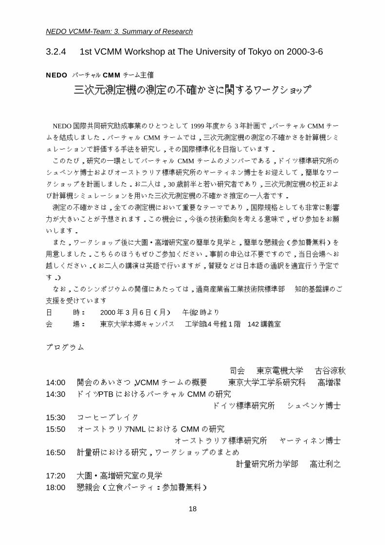
3.2.4 1st VCMM Workshop at The University of Tokyo on 2000-3-6 NNEEDDOO ババーーチチャャルル CCMMMM チチーームム主主催催

三三次次元元測測定定機機のの測測定定のの不不確確かかささにに関関すするるワワーーククシショョッッププ

NEDO 国際共同研究助成事業のひとつとして 1999 年度から 3 年計画で，バーチャル CMM チー

ムを結成しました．バーチャル CMM チームでは，三次元測定機の測定の不確かさを計算機シミ

ュレーションで評価する手法を研究し，その国際標準化を目指しています．

このたび，研究の一環としてバーチャル CMM チームのメンバーである，ドイツ標準研究所の

シュベンケ博士およびオーストラリア標準研究所のヤーティネン博士をお迎えして，簡単なワー

クショップを計画しました．お二人は，30 歳前半と若い研究者であり，三次元測定機の校正およ

び計算機シミュレーションを用いた三次元測定機の不確かさ推定の一人者です．

測定の不確かさは，全ての測定機において重要なテーマであり，国際規格としても非常に影響

力が大きいことが予想されます．この機会に，今後の技術動向を考える意味で，ぜひ参加をお願

いします．

また，ワークショップ後に大園・高増研究室の簡単な見学と，簡単な懇親会（参加費無料）を

用意しました．こちらのほうもぜひご参加ください．事前の申込は不要ですので，当日会場へお

越しください．（お二人の講演は英語で行いますが，質疑などは日本語の通訳を適宜行う予定で

す．）

なお，このシンポジウムの開催にあたっては，通商産業省工業技術院標準部知的基盤課のご

支援を受けています

日時： 2000 年 3 月 6 日（月）午後 2 時より

会場：東京大学本郷キャンパス工学部 14 号館 1 階 142 講義室

プログラム

司会東京電機大学古谷涼秋 14:00 開会のあいさつ，VCMM チームの概要東京大学工学系研究科高増潔 14:30 ドイツ PTB におけるバーチャル CMM の研究ドイツ標準研究所シュベンケ博士 15:30 コーヒーブレイク 15:50 オーストラリア NML における CMM の研究オーストラリア標準研究所ヤーティネン博士 16:50 計量研における研究，ワークショップのまとめ計量研究所力学部高辻利之 17:20 大園・高増研究室の見学 18:00 懇親会（立食パーティ：参加費無料）


19

講師紹介

Dr. Heinrich Schwenke ドイツ標準研究所（Physikalisch-Technische Bundesanstalt）

1995 年 TU Braunschweig で修士 "Design of a Spindelless Instrument for the Roundness

Measuring of Ultraprecision Ball"

1999 年 PhD "Assessing Measurement Uncertainties by Simulation in Dimensional Metrology"

1995 年より PTB で CMM キャリブレーション，マイクロマシン用センサの開発，シミュレーシ

ョン法による CMM の不確かさ解析の研究に従事，現在は，Head of Coordinate Metrology Section．

Dr. Esa Jaatinen

オーストラリア標準研究所（National Metrology Laboratory）

1990 年 University of Queensland を卒業

1994 年 Australian National University で PhD "Nonlinear Optics"

1994 年より NML にて波長標準の開発と研究に従事，現在は CMM の理論的な研究および CMM

の幾何誤差とボールプレートの干渉法による校正を担当．


20

3.2.5 2nd VCMM Workshop at NMIJ on 2000-8-28 NNEEDDOO ババーーチチャャルル CCMMMM チチーームム主主催催

第第 22 回回三三次次元元測測定定機機のの測測定定のの不不確確かかささにに関関すするるワワーーククシショョッッププ

NEDO 国際共同研究助成事業のひとつとして 1999 年度から 3 年計画で，バーチャル CMM チー

ムを結成しました．バーチャル CMM チームでは，三次元測定機の測定の不確かさを計算機シミ

ュレーションで評価する手法を研究し，その国際標準化を目指しています．

3 月には，研究の一環としてドイツ標準研究所のシュベンケ博士およびオーストラリア標準研

究所のヤーティネン博士をお迎えして，第 1 回ワークショップを東京大学で開催しました．今回

は，やはりバーチャル CMM チームのメンバーである，ドイツ標準研究所のベルデル博士，シュ

ベンケ博士，オーストラリア標準研究所のブラウン博士および特別に米国標準研究所のシャカル

ジ博士をお迎えして，第 2 回ワークショップをつくば国際会議場｢エポカルつくば｣で開催いたし

ます．

講演者は，すべて三次元測定機の校正および計算機シミュレーションを用いた三次元測定機の

不確かさ推定の一人者です．計量研究所を含めた 4 つの主要標準研究所から三次元測定機関係の

責任者が集まり，今後の国際規格の動向などの紹介と議論を行います．測定の不確かさは，全て

の測定機において重要なテーマであり，国際規格としても非常に影響力が大きいことが予想され

ます．この機会に，今後の技術動向を考える意味で，ぜひ参加をお願いします．事前の申込は不

要ですので，当日会場へお越しください．（講演は英語で行いますが，質疑などは日本語の通訳を

適宜行う予定です．）

なお，このシンポジウムの開催にあたっては，通商産業省工業技術院標準部知的基盤課のご

支援を受けています．

講演者紹介

Dr. Franz Wäldele Head of Department “Measuring Instruments Technology” ドイツ標準研究所（PTB）長さ測定関係の責任者

Dr. Heinrich Schwenke Head of Coordinate Metrology Section ドイツ標準研究所（PTB）三次元測定関係の責任者

Dr. Nickolas Brown Leader, Length Standards Project オーストラリア標準研究

所（NML） APMP の長さ関係の責任

者

Dr. Craig Shakarji Manufacturing System Integration Division 米国標準研究所（NIST） ISO 15530-3（シミュレー

ション法）のグループリー

ダー


21

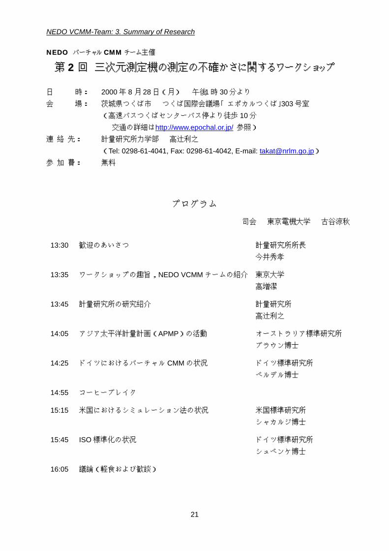
NNEEDDOO ババーーチチャャルル CCMMMM チチーームム主主催催

第第 22 回回三三次次元元測測定定機機のの測測定定のの不不確確かかささにに関関すするるワワーーククシショョッッププ日時： 2000 年 8 月 28 日（月）午後 1 時 30 分より会場：茨城県つくば市つくば国際会議場｢エポカルつくば｣ 303 号室（高速バスつくばセンターバス停より徒歩 10 分交通の詳細は http://www.epochal.or.jp/ 参照）連絡先：計量研究所力学部高辻利之（Tel: 0298-61-4041, Fax: 0298-61-4042, E-mail: [email protected]）参加費：無料

プログラム

司会東京電機大学古谷涼秋

13:30 歓迎のあいさつ計量研究所所長今井秀孝

13:35 ワークショップの趣旨，NEDO VCMM チームの紹介東京大学高増潔

13:45 計量研究所の研究紹介計量研究所高辻利之

14:05 アジア太平洋計量計画（APMP）の活動オーストラリア標準研究所

ブラウン博士

14:25 ドイツにおけるバーチャル CMM の状況ドイツ標準研究所ベルデル博士

14:55 コーヒーブレイク

15:15 米国におけるシミュレーション法の状況米国標準研究所シャカルジ博士

15:45 ISO 標準化の状況ドイツ標準研究所シュベンケ博士

16:05 議論（軽食および歓談）


22

3.2.6 3rd VCMM Workshop at Melbourne on 2002-2-26

NEDO VCMM-Team: 4. Research Reporst by Members

23

4. Research Report by Members

4.1 Research Report by the University of Tokyo Kiyoshi Takamasu, The University of Tokyo

During the NEDO VCMM project (time from 1999-2002), the theoretically study and research for Virtual CMM method has been done at the University of Tokyo. We established the basic theories for estimating the uncertainty of measurement in coordinate metrology. The main work items have been:

- Establishment of concept of feature-based metrology for estimating the uncertainty of measurements in coordinate metrology.

- Establishment of evaluation method for effect of unknown systematic errors

1. Establishment of concept of feature-based metrology

1.1 Introduction

In coordinate metrology, an associated feature is calculated from a measured data set on a real feature by CMM (Coordinate Measuring Machine). Then, the associated features are compared with the nominal features which are indicated on a drawing (see figure 1). In this data processing, the features are primal targets to calculate, to evaluate and to process. Consequently, this process is called as “Feature-Based Metrology”.

Nominal feature

Real feature

Extracted feature

Associated feature

Nominal derived feature

Extracted derived feature

Associated derived feature

Figure 1. Data processing flow in feature based metrology

1.2 Uncertainty of feature

The uncertainty of each measured point is defined by error analysis of CMM and probing system, and the results of profile measurement on each feature. From the uncertainty of measured point, the uncertainty of measured feature can be calculated statistically using following equations.

Equation (1) shows an observation equation, a regular equation and a least squares solution, where A is Jacobian matrix, p is a parameter vector and S is an error matrix.

NEDO VCMM-Team: 4. Research Reports by Members

24

dSAASApdSAApSA

Apd

11

11

)( :solution squaresleast :equationreguler

:equationn observatio

−−

−−

=

=

=

tt

tt (1)

Using the propagation law of error to least squares method, the error matrix of parameter Sp, and the error matrix of observation Sm are calculated as equations (2) and (3) respectively. The matrices Sp and Sm indicate the variations of the parameters and the values of observation equations at each position.

11p )( −−= ASAS t (2)

tpAASS =m (3)

Figure 2 shows an example of error analysis form twelve measured points on a flat plane. Middle plane is least squares plane, the upper and the lower planes are the upper and the lower limits of confidential zone of feature respectively. We note that the upper and the lower limits of confidential zone is equal to the range of the uncertainty of measured feature. Using equation (3), the uncertainty at the position out of measuring range also can be calculated.

Measured points

Least squares

Confidential zone

2

−2

0

Z Y

X

Figure 2. Confidential zone of measure plane; number of measured points is 12 and standard deviation of each measured point is 1.0.

1.3 Conclusions and future works

In this research, we have placed basic concept of feature based metrology which is used in coordinate metrology and constructed the data processing flow of it using CMM. From theoretical analysis, we reach the following conclusions:

1. least squares method is suited to calculate the geometric parameters and the uncertainty of features,

2. simple (low degree) model is fitted to the model of feature in the condition of feature based metrology,


25

3. calculation method of the uncertainty of feature is presented using least squares method and statistical evaluation,

4. calculation method of the uncertainty of related feature is also presented.

The future works in feature based metrology as follows: 1. how to define uncertainty of each measured point in CMM, 2. how to select the model of each feature; evaluating function of selection, 3. how to evaluate of the results of measurement; how to compare geometric

parameters and tolerancing, 4. how to decide the strategy of measurement using feature based metrology.

2. Establishment of evaluation method for effect of unknown systematic errors 2.1 Introduction In this research, the effects of systematic errors are theoretically analyzed to estimate the uncertainties in feature-based metrology. The center position error and the diameter error of the ball probe are taken up for the examples of the effects of systematic errors. These errors are occurred from the random errors of probing in calibration process and propagate as unknown systematic errors to the uncertainties of measured parameters such as the center position and the diameter of a measured circle.

Figure 3 shows the model for the theoretical analysis. Firstly, diameter and center position of a probe ball are calibrated by measuring a reference circle. The diameter of the reference circle is calibrated with the uncertainty sc. After the calibration, a measured circle is measured by the ball probe with random measured error sp.

When the only random errors are put in the consideration and n measured points are probed uniformly on the measured circle, the uncertainties of measured diameter and center position of the measured circle can be calculated as equations (4), (5), (6) and (7) using equations (2) and (3). Where the position of probed point is displayed by ti and ri in figure 4.

11

2

2

2

)( −−=

= ASAP t

dydxd

ydyxy

xdxyx

sssssssss

(4)

=

=10

01

0

02

2

2

OO p

p

p

ss

sS (5)

−−−

−−−

=

21sincos

21sincos 11

nn tt

tt

MMMA (6)


26

=

2

2

2

400

020

002

p

p

p

sn

sn

sn

P (7)

Calibration of center position and diameter of ball

X

Y

Ball probe

Ball probe

Measurement of center position and diameter of circle

Measured circle

Reference circle

Ball probe

Measured circle

ti

ri

X

Y

Figure 3. Model for calibration of ball probe and Figure4. Measured positions by angle ti

measurement of circle

2.2 Unknown systematic errors From the calibration process of the ball probe, the unknown systematic errors of diameter and center position of the ball probe are occurred. The effect of these unknown systematic errors is not same as the effect of the random errors.

2.2.1 Unknown systematic errors from diameter of ball probe Figure 5 displays the influences of uncertainty of the diameter of the ball probe for the step measurement and size measurement. The uncertainty of diameter effects the only size measurement. Figure 6 and equation (8) show the measuring errors dr1 and dr2 from diameter errors on the measured circle. The variance and the covariance from diameter errors are shown in equation (9), where cd is diameter error. In this case the error matrix of the parameters is calculated as equation (10).

2

2

22

11

dpdr

dpdr

+=

+= (8)

4

42

212

222

221

d

dp

cs

csss

=

+== (9)


27

+

=

22

2

2

400

020

002

dp

p

p

csn

sn

sn

P (10)

Normal vector

Step Size

Ball probe

X

Y

dr1 = p1 + d/2

Measured circle

dr2 = p2 + d/2Ball probe

Figure 5. Effect of diameter errors of ball probe Figure 6. Correlation of two measured on step dimension and size dimension points by effects from diameter error

2.2.2 Unknown systematic errors from center position of ball probe Figure 7 displays the influences of uncertainty of center position of the ball probe. Figure 8 and equation (11) show the measuring errors dr1 and dr2 from center position errors on the measured circle. The variance and the covariance from center position errors are shown in equation (12), where cx is center position error.

222

111

sincossincos

tdytdxdrtdytdxdr

+=+=

(11)

)cos(

sinsincoscos

sincos

212

212

2122

12

21

221

2222

21

ttc

ttcttcs

ctctcss

x

yx

xyx

−=

+=

=+==

(12)

dx

dy dr

X

Y t

Ball probe

Measured object

dr1

X

Y

t1 − t2

dr2

Measuredobject

Ball probe


28

Figure 7. Effect of center position errors of ball Figure 6. Correlation of two measured probe points by center position errors

2.3 Conclusions In this research, we theoretically analyzed the effects of the unknown systematic errors in feature-based metrology. The center position error and the diameter error of the ball probe are occurred from the random errors of probing in calibration process. These errors propagate as unknown systematic errors to the uncertainties of measured parameters such as the center position and the diameter of a measured circle. The method to calculate the error matrix was derived when the center position and the diameter of the circle are measured.

Using this method, the uncertainties of the measured parameters can also be calculated in the complex measuring strategy. The series of simulations for this method in statistical way directly implies that the concept and the basic data processing method in this paper are useful to the feature based metrology.


29

4.2 Research Report by Tokyo Denki University

Ryoshu FURUTANI, Tokyo Denki University

1 Introduction Virtual CMM was a hot topics in a working group 10 in ISO/TC213 in 1998. At that moment, ISO/TC213/WG10 concentrated to finalize the document ISO 10360 series, which described verification and reverification test of CMM. In WG10, we discussed how to estimate the uncertainty of CMM measurement and determined the following document series. 15530-1: Terms 15530-2: Expert Judgment 15530-3: Substitution Method 15330-4: Simulation Method 15330-5: Historical Estimation 15530-6: Estimation using Uncalibrated objects. In these documents, only 15530-3 and 15530-4 seemed to estimate the uncertainty of CMM measurement. This was our feeling. When the simulation method would be on the table in WG10, we would have to decide to support it or not. However nobody knew the details of simulation method. So we had selected the VCMM as one of possible simulation method and proposed the collaborated research work to PTB. Now ISO/TC213/WG10 continues the process to issue the ISO 15530-4. 2 Purpose Our purpose was 1) understanding the details of VCMM. 2) understanding How VCMM estimate the uncertainty of measurement. 3 Result 3.1 Translation of document of VCMM

We translated the document “Traceability of Coordinate Measurements According to the Method of the Virtual Measuring Machine” to Japanese. In the process of translation, we discussed the technical details and we could understand the details of VCMM. After understanding the details of VCMM, we had two new questions.


30

1) The estimated uncertainty by VCMM is adequate or not ? 2) It is difficult to build simulation software(VCMM) or not? To make these questions clear, I had built VCMM software by myself. 3.2 Building VCMM Software

In Simulation software, it is most import to determine what type of the model can be handled. Generally, the model of CMM are following, 1) including geometrical errors 2) including dynamic behaviors 3) including temperature effects 4) including probing effects. In our simulation method, we did not want to add any additional sensors to CMM. So we could not handle 3). The model 2) requires more the calibrated artifacts and information of errors. Finally we could handle only geometrical errors and probing effects. In this simulation software, we had implemented two kind of probing effects, which are the random probing effects and the spherical harmonics probing effects. The traditional probing system of CMM has the spherical harmonics probing effects. The geometrical errors were extracted by KALKOM, which is a software for extracting the geometrical errors from measurement result of the ball/hole plate. It can extract only the geometrical errors and can not extract any uncertainty of geometrical errors. The simulation software was described in Matlab script language. The implementation of simulation software was not more difficult than understanding the details. 3.3 Execution of simulation software

The simulation software requires the definition of CMM, measuring program and measured points. The definition of CMM are kinematical model of CMM, geometrical errors of CMM and probing effects as above section. The measuring program are dependent on the workpiece. The measured points are dependent on the

% Plane 100 100 100 0 0 -1 200 200 100 0 0 -1 0 200 100 0 0 -1 100 300 100 0 0 -1 % Circle 100 100 100 0 -1 0 200 200 100 1 0 0

Figure 1 Example of measured points


31

actual measurements. In this implementation, the measured points, the measuring program are stored in the files. Figure 1 shows an example of measured points. Each line means one measured point. First three values mean x,y,z coordinate of measured points. Next three points mean the probing vector of measured points. This information is used to distinguish the inner circle and the outer circle and so on. The beginning of % means the comment line. Figure 2 shows an example of measuring program. This line means measuring circle by

cmm_circle(64,[[0,0,0];[0,0,1]])

;

Figure 2 Example of measuring program

%%%%%%%%%%%%%%%%%%%%%%%%%%%%%%%%%%%%%%%%%%%%%%%%% % VCMM Report Date:21-Feb-2002 % VCMM Version: dickson tuned on 25-02-2001 %%%%%%%%%%%%%%%%%%%%%%%%%%%%%%%%%%%%%%%%%%%%%%%%%% % Configulation % Cmm: cmm_falcio % Probe:probe_ph10 % Errors:TDU-BALL\TDU-result.exc %%%%%%%%%%%%%%%%%%%%%%%%%%%%%%%%%%%%%%%%%%%%%%%%%% % VCMM Options % Probe:Harmonics + Random Error % CMM Geometric Deviation:Deviation % CMM Uncertainty:No Uncertaity % Interpolation:Linear Interpolation %%%%%%%%%%%%%%%%%%%%%%%%%%%%%%%%%%%%%%%%%%%%%%%%%% % VCMM Command: meas_command_1 % VCMM Points: meas_points_1 % Number of Simulation:10 %%%%%%%%%%%%%%%%%%%%%%%%%%%%%%%%%%%%%%%%%%%%%%%%%% res_1:cmm_circle(64,[[0,0,0];[0,0,1]]) ;

Measurand 0.000000 0.000000 0.000000 11.281400 0.000000 0.000000 0.000000 Mean 0.011394 -0.001181 0.000000 11.281555 0.011394 -0.001181 0.000000 Uncertainty 0.011601 0.001374 0.000000 0.000311 0.011601 0.001374 0.000000 Sigma 0.000104 0.000096 0.000000 0.000078 0.000104 0.000096 0.000000

Figure 3 Example of output from simulation software


32

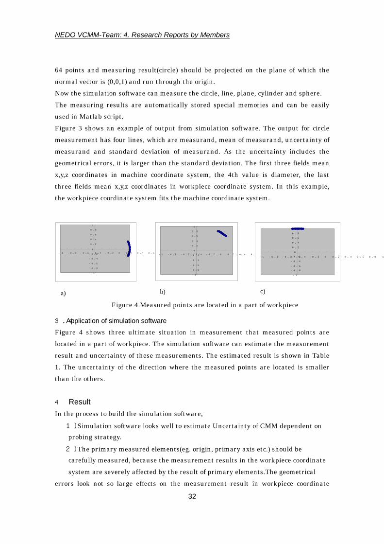
64 points and measuring result(circle) should be projected on the plane of which the normal vector is (0,0,1) and run through the origin. Now the simulation software can measure the circle, line, plane, cylinder and sphere. The measuring results are automatically stored special memories and can be easily used in Matlab script. Figure 3 shows an example of output from simulation software. The output for circle measurement has four lines, which are measurand, mean of measurand, uncertainty of measurand and standard deviation of measurand. As the uncertainty includes the geometrical errors, it is larger than the standard deviation. The first three fields mean x,y,z coordinates in machine coordinate system, the 4th value is diameter, the last three fields mean x,y,z coordinates in workpiece coordinate system. In this example, the workpiece coordinate system fits the machine coordinate system.

3.4 Application of simulation software

Figure 4 shows three ultimate situation in measurement that measured points are located in a part of workpiece. The simulation software can estimate the measurement result and uncertainty of these measurements. The estimated result is shown in Table 1. The uncertainty of the direction where the measured points are located is smaller than the others. 4 Result In the process to build the simulation software,

1) Simulation software looks well to estimate Uncertainty of CMM dependent on probing strategy. 2) The primary measured elements(eg. origin, primary axis etc.) should be carefully measured, because the measurement results in the workpiece coordinate system are severely affected by the result of primary elements.The geometrical

errors look not so large effects on the measurement result in workpiece coordinate

-1

-0.8

-0.6

-0.4

-0.2

0

0.2

0.4

0.6

0.8

1

-1 -0.8 -0.6 -0.4 -0.2 0 0.2 0.4 0.6 0.8 1

a)

-1

-0.8

-0.6

-0.4

-0.2

0

0.2

0.4

0.6

0.8

1

-1 -0.8 -0.6 -0.4 -0.2 0 0.2 0.4 0.6 0.8 1

b)

-1

-0.8

-0.6

-0.4

-0.2

0

0.2

0.4

0.6

0.8

1

-1 -0.8 -0.6 -0.4 -0.2 0 0.2 0.4 0.6 0.8 1

c)

Figure 4 Measured points are located in a part of workpiece


33

system, because the output in workpiece coordinate system is calculated from the difference between the coordinates of two objects and the errors are localized.

c)

b)

a)

0.153357 0.155764 0.018935 unc.

3.027374 -0.966708 0 measurand

0.101738 0.079618 0.075418 unc.

2.333673 -0.341425 0.280714 measurand

0.026785 0.004527 0.019993 unc.

1.716762 0 0.783095 measurand diameter y x

Table 1 Estimated result when the measured points are located in a part of workpiece


34

4.3 Research Report by National Metrology Institute of Japan

AIST, NMIJ, T. Kurosawa and T. Takatsuji 1. Introduction

In order to assess the uncertainty of the coordinate measurement based on simulation methods, the characteristics of the target coordinate measuring machine (CMM) should be evaluated with an aid of a calibrated gauge in advance. The uncertainty of the calibration of the gauge contributes to the uncertainty of the coordinate measurement directly; hence it is important to calibrate the gauge accurately and with traceability.

Taking advantage of the fact that the AIST is a national metrology institute responsible for national standard, we were going to take part in this international project and contribute to the standardization of the simulation method mainly by calibrating the gauges.

Main research items are analysis of calibration uncertainty of a ball plate using gauge blocks, development and calibration of a ball step gauge, international comparison of gauges, international comparison of the measurement of workpieces, and so on. In the following sections, these research items will be explained.

2. Analysis of calibration uncertainty of a ball plate using gauge blocks

The characteristic of the target CMM, which is used in the simulation method, is normally evaluated using a ball plate or a hole-plate. The ball plate is a steel plate in which steel or ceramic spheres are buried on grid positions as shown in figure 1, and the positions of the spheres should be calibrated accurately.

The ball plate is calibrated using a CMM. At the last step of the calibration procedure, the measurement values are compared with the measurement values of the gauge blocks and compensated to keep the traceability to the length standard.

We found that the probing error of the CMM is involved in the calibration

Figure 1 Ball plate


35

result in this compensation procedure; therefore we proposed a method of using multiple gauge blocks to avoid this problem. This method was theoretically investigated to show its validity, and its efficiency in the calibration of the ball plate was demonstrated. Detail of this method is explained in the references.

3. Development and calibration of a ball step gauge

Although the ball plate can be calibrated with the aid of gauge blocks as explained above, it is ideal to transfer the length standard from a subsidiary gauge, which has the same shape as the ball plate, to the ball plate.

Hence a ball step gauge was developed as shown in figure 2, which has one-dimensional shape of the ball plate. The ball step gauge has H-shaped cross-section and the spheres are aligned in its neutral plane. Owing to this structure the ball step gauge is rigid against deformation due to heat or mechanical stress.

Additionally the subsidiary gauge should be directly calibrated from the laser, which is the length standard. An interferometric stepper enables to do so; hence it is one of the ideal gauges as a subsidiary gauge used for the calibration of the ball plate. Detail of the ball step gauge is explained in the references.

4. International comparison of the

calibration of the gauges

Only one way of checking the validity of the calibration of the gauges is an international comparison. Not only the AIST as a Japanese national metrology institute (NMI) but the PTB as a German NMI and the NML as an Australian NMI took part in this project. All of these laboratories are top-level NMIs in the world. The result of the international comparison carried out by these three NMIs is sufficient to prove the validity of the calibration of the gauges.

Three laboratories have their own hole-plates as shown in figure 3. These three hole-

Figure 2 The ball step gauge and the interferometric stepper


36

plates were measured by three laboratories; i.e. each hole-plate was measured three times. The result of this comparison will be reported in sections c and g. Good results have been obtained in all measurements, and it indicates the capability of the calibration of the three laboratories. Additionally the uncertainty of the calibrated values of the hole-plates is small enough to use for characterizing the geometrical error of the CMM.

5. International comparison of the

measurement of the workpieces

Although the title of this project is VCMM, we have been researching on simulation methods for assessing the uncertainty of coordinate measurement. Many simulation methods including VCMM are currently available. In this project, Prof. Furutani and Dr. Jaatinen made their original simulation methods.

We made two sample workpieces and planed an international comparison using the workpieces to observe the difference of various simulation methods. Details of the international comparison will be explained in section h.

Currently the sample workpieces are being circulated in participant laboratories.

6. Other activities

On March 2000, a part of the members gathered in National Research Laboratory of Metrology (NRLM, former institute of AIST) in Japan, and performed a joint experiment on the characterization of the geometrical errors of the CMM and VCMM.

Dr. Takatsuji visited PTB on April 2000 and exchanged the information about the calibration of geometrical gauges.

Dr. Kurosawa organized the second project meeting held in Japan on July 2000.

Figure 3 The hole-plate


37

Taking advantage of this opportunity, he also organized the workshop for Japanese industries to disseminate the simulation methods and advertise the project. Dr. Takatsuji played a role of an assistant.

Dr. Takatsuji has attended the ISO meeting several times and put an effort to standardize the simulation method.

Both Dr. Kurosawa and Dr. Takatsuji attend monthly project meeting held in Japan to have discussions and exchange information on the simulation methods.

Both of them attended many international and domestic conferences.

7. Conclusions

With the support of NEDO, the simulation methods have been more popular in these three years and its standardization is progressed. It is a matter of time to become a formal ISO standard. We would like to express our greatest gratitude to NEDO.


38

4.4 Research Report by Physicalish-Technishe Bundesanstalt

Franz Waldele, Heinrich Schwenke, PTB, Germany

During the time from 1999-2002 the development and dissemination of the Virtual CMM has been one of the key activities of the laboratory for CMM at PTB. In this time, we made significant progress both in the technical development and the proliferation to industry. The following report summarizes the main activities within and outside the NEDO project and lists the main achievements. The main work items have been:

Work items within the NEDO project:

- Standardization of the VCMM

- Establishment of an International Network on CMM research

- Installation of the VCMM in Japan and Australia

- Comparison of Hole Plate calibrations

- Manufacturing of primary Hole Plate standards for NMIJ and CSIRO

- Dissemination of VCMM methods to the scientific and industrial community

Work items concerning the Virtual CMM outside the NEDO project:

- Establishment of a calibration service for prismatic parts based on the VCMM

- Improvement of VCMM software routines

- Development of new software tools for the VCMM

- Preparation of Quality Manuals and procedures for the Virtual CMM

In the following these work items are shortly summarized.

Standardization of the VCMM During the project, a draft for an international standard for uncertainty calculation based on simulation has been prepared and made a priority work item for the ISO group TC213/WG10. The task force consists of two NEDO


39

members and a delegate from the US. In several productive meetings the general concept was developed and a comprehensive draft was produced and extensively discussed in ISO. Additionally, an national German guideline VDI 2617-7 was produced and already published as a draft.

Establishment of an International Network on CMM research In several meetings in Germany, Japan and Australia a close international network for CMM research has been established. Workshops, presentations and discussions not only resulted in an effective professional know-how transfer, but also in a very good personal relationship between the NEDO members, which will be a solid base for future collaborations. This network already produced important contacts on the field of laser trackers for CMM calibration and on internet based monitoring of CMMs.

Installation of the VCMM in Japan and Australia Calibration of the CMMs in NMIJ and CSIRO were performed and the VCMM was installed at both laboratories. First measurements have been performed which delivered promising results. The staff in both laboratories was trained in the calibration of CMM using ball plates, the operation of the Virtual CMM and in the scientific background.

Comparison of Hole Plate calibrations Comparison of Hole Plate calibrations have been performed between NMIJ, CSIRO and PTB. The results document the ability of all laboratories to perform calibration of Hole Plates within their stated uncertainties. During the project, NMIJ and CSIRO have optimized their calibration procedures to a very high degree of confidence. The results of the comparison were documented in a report.

Manufacturing of primary Hole Plate standards for NMIJ and CSIRO In collaboration of the NEDO members with the German company SCHOTT two state-of-the-art Hole Plate Standards have been manufactured. These Hole Plates have and unprecedented surface quality and long term stability. They will serve as primary standards for NMIJ and CSIRO.


40

Dissemination of VCMM methods to the scientific and industrial community During a number of seminars and workshops on three continents the VCMM method was disseminated to the scientific and industrial community. Many publications and conference contributions have been made concerning the VCMM. The publications are documented and supplied as an addendum to this final report.

Establishment of an calibration service for prismatic parts based on the VCMM One of the major achievements in the national context is the establishment of a calibration service in the German industry based on the VCMM. Eight private laboratories have calibrated their CMMs according to this method and have installed the VCMM to produce task related uncertainty statements. Not less than 10 000 measurements of different parameters on different objects employing different probing strategies have been performed to validate the method. The results confirm the feasibility and correctness of the approach. For the end of 2002, the accreditation of 6 laboratories within the DKD (German Calibration Service) is scheduled.

Improvement of VCMM software routines The simulation routines have been improved concerning completeness, handling, and transparency. Two new uncertainty contributors have been included and verified: Relative probe calibration uncertainty and surface roughness contribution. The simulation core now produces detailed debug information files. The interfaces to the manufacturers software have been extended. The manufacturers have improved the integration of the VCMM routines significantly. The operation is simplified.

Development of a new software tool for the VCMM A new software tool has been developed to improve the generation and the management of the VCMM input data, the so called “VCMM Tool”. It can visualize the input data including all geometric uncertainty contributors and


41

helps the user to generate input data by specialized “assistants”. Furthermore, this tool can perform simulations of length measurements on a specific CMM to generate a global “accuracy parameter” of the machine. The new tool contributes to an increased transparency of the method and makes the generation of new uncertainty scenarios a lot easier.

Production of Quality Manuals and procedures for the Virtual CMM As an important prerequisite for the implementation of the virtual CMM in quality systems the procedures and quality manuals have been prepared and discussed with our industrial partners. These procedures are now compulsory for workpiece calibrations in PTB and have been a template for the documentation in the DKD laboratories.


42

4.5 Research Report by National Measurement Laboratory, CSIRO

Nicholas Brown, Esa Jaatinen, CSIRO, NML, Australia

Functions and responsibilities CSIRO’s responsibility for maintaining the nation’s primary physical standards is identified in two Acts of Parliament, the Science and Industry Research Act 1949 and the National Measurement Act 1960. Under the Science and Industry Research Act 1949, CSIRO is required to establish, develop and maintain standards of measurement of physical quantities and, in relation to those standards: (i) to promote their use; (ii) to promote, and participate in, the development of calibration with respect to them; and (iii) to take any other action with respect to them that the Executive thinks fit. Under the National Measurement Act 1960, the Organisation shall maintain, or cause to be maintained: (i) such standards of measurement as are necessary to provide means by which measurement of physical quantities for which there are Australian legal units of measurement may be made in terms of those units; and (ii) such standards of measurement (not being Australian primary standards of measurement) as it considered desirable to maintain as Australian secondary standards. The Organisation's responsibilities are discharged through NML. Current Research Activities 1. Development of a Virtual Coordinate Measuring Machine with NMIJ

(Japan) and PTB (Germany). 2. New Microwave frequency standard based on Laser-Cooled 171Yb+ Ions 3. New high-accuracy deadweight pressure standard 4. Development of a new current Quantized Hall Resistance


43

Development of a Virtual Coordinate Measuring Machine/ new measurement techniques. Software has been developed at NML to determine CMM uncertainties using a different approach to the Virtual CMM software developed at PTB in Germany. This is called OzSim and uses a simpler approach to the VCMM software but can be applied to more complex situations. It has shown good agreement with the VCMM results. New probing techniques are being investigated to compare mechanical probing with laser interferometry. This is important for traceability. The probe position is monitored with a laser interferometer as the probe approaches the contact surface and after contact. Elastic changes are observed and are being investigated to allow “zero force” probing. A web page has been established to provide information on the VCMM work and can be found at (http://www.metrologu.asn.au/cmmgroup.htm) Recent publications:

• "Temperature of Laser-Cooled 171Yb+ Ions and Application as a

Microwave Frequency Standard" - R.B. Warrington, P.T.H. Fisk, M.J. Wouters and M.A. Lawn

MSA Conference, Gold Coast, 2-4 October 2001 • “A New Facility at NML for the Development of Reference Gas Mixtures as

a Part of the Australian Metrology Infrastructure” – G de Groot, M Arnautovich, S Rennie and L Besley

• “International Metrology – Recent Developments in Mutual Recognition of National Metrology Institutes” – G Sandars

• “Optimizing CMM Measurement Processes by Calculating the Uncertainty” – E Jaatinen, R Yin, M Ghaffari and N Brown

• “Uncertainty Estimation for a Novel Pendulum” – R Cook and W Giardini


44

• “Static Torque Instrument Calibration” – I Bentley (NATA) and J Man

• “Algorithm and Uncertainty of AC-DC Transfer Measurements” – I Budovsky

• “Development of a Cryogenic Comparator System at NML” – B Pritchard

• “Measurement of Temperature, Humidity and Pressure Coefficients of Zener-Based Voltage Standards” – R Frenkel

• “Automation of a Pressure Controlled Heatpipe for Use as a Thermometer Calibration Enclosure” – M Ballico

• “Calibration of Thermometers for Hygrometry in a Temperature-Controlled Chamber” – K Chahine, N Bignell and E Morris

• “A Miniature Copper Point Crucible for Thermocouple Calibration” – M Ballico, F Jahan and S Meszaros

• “The NML-Australian Definition of the Kelvin” – M Ballico and K Nguyen

• “The Piston Cylinder Pressure Gauge” – W Giardini and B Triwiwat

• “A New Solid Density Standard with a Relative Uncertainty of 1 in 107” – K Fen, E Jaatinen, B Ward and M Kenny

• “A Comparison of Roundness Measurements Between Australia and Indonesia” – A Baker

• “How Well Can We Provide Uncertainties for CMM Measurements?” – R Yin, E Jaatinen, M Ghaffari and N Brown

• “Uncertainty Analysis of the Chemical Composition of Reference Gas Mixtures Created by the Gravimetric Method” – M Arnautovich, G de Groot and L Besley

• “Facility at NML to Provide Traceability for Low-Frequency EMC Tests” – G Hammond and I Budovsky

• “The Measurement of RF-DC Difference 1 MHz to 100 MHz” – S Grady

• “Propagation of Correlations Down the Traceability Chain” – J Gardner

• “Thermal Effects in Small Sonic Nozzles” – N Bignell, Y Choi (KRISS, Korea)

• “Automation of Calibration in Hygrometry” – K Chahine

• Bruce Warrington presented a paper entitled “A Microwave Frequency Standard based on Laser-cooled 171Yb+ Ions” at the 6th Symposium on


45

Frequency Standards and Metrology, St Andrews, Scotland, during the week 10-14 Sept.

• Yi Li presented two papers at the 12th International Symposium on High Voltage Engineering in Bangalore, India (20-24 August), entitled , "Frequency Composition of Lightning Impulses and K-Factor Filtering" –

• Y Li and J Rungis, and “The Contribution of Software to the Uncertainty of Calibrations of Calibration Pulse Generators” – T McComb and Y Li.

Seminars / Workshops

• Calculation of Measurement Uncertainty using the Monte Carlo Method:

Seminar at PTB, Germany, 17-18 June 2001

• N. Brown “The NML team and what we can provide for industry”, CMM traceability & the Virtual CMM- A workshop for industry held in Melbourne on 26 February 2002

NEDO VCMM-Team: 5. Collaboration Reports

46

5. Collaboration Reports 5.1 Comparison measurement on prototype Hole Plate

Heinrich Schwenke, PTB Scope PTB provided a calibrated prototype Zerodur Hole Plate as part of the NEDO project to allow both NRLM and NML to determine their CMM measuring capabilities. The plate was first sent to NML, where it was measured over a period of two weeks from the 28th of January 2000 to the 9th of February 2000 before being shipped to Japan, where it was measured during the following month. The plate is 450 mm x 450 mm x 31.1 mm and its serial number is PTB 5.32 3/97. The last PTB calibration sticker is 3319. There are fifty-six holes in the plate and all of them have a nominal diameter of 30 mm. The holes are arranged in rows and columns that are parallel to defined 'U' and 'V' orthogonal axes on the plate. The spacing of the holes in the two outer rows and two outer columns is 40 mm but twice that (80 mm) for the holes in the inner rows and columns. No calibration values were supplied with the plate.

Photo Hole Plate


47

Results The measured coordinates of NML and NRML were send to PTB and a comparison of calibration values was performed at PTB. Figure 2 and 3 show the results.

Figure 1: Direct comparison X-coordinate

Figure 2: Direct comparison Y-coordinate

-0.0008

-0.0006

-0.0004

-0.0002

0.0000

0.0002

0.0004

0.0006

0 50 100 150 200 250 300 350 400 450

X-Coordinate

Dev

iatio

n NMIJ-PTBCSIRO-PTBCSIRO-NMIJ

-0.0012

-0.0010

-0.0008

-0.0006

-0.0004

-0.0002

0.0000

0.0002

0.0004

0.0006

0.0008

0 50 100 150 200 250 300 350 400 450

Y-Coordinate

Dev

iatio

n NRLM-PTBCSIRO-PTBNRLM-CSIRO


48

-50

0

50

100

150

200

250

300

350

-50 0 50 100 150 200 250 300 350 400 450 500

Y (m

m)

X (mm)

14. May. 2002 16:31

scal

e of

dev

iatio

ns0.

0004

Programm TRANSFORM

Figure 3: Comparison CSIRO-PTB after best fit in orientation

-50

0

50

100

150

200

250

300

350

-50 0 50 100 150 200 250 300 350 400 450 500

Y (m

m)

X (mm)

15. May. 2002 13:16

scal

e of

dev

iatio

ns0.

0004

Programm TRANSFORM

Figure 4: Comparison NMIJ-PTB after best fit in orientation


49

Comparing the data, the following observations have been made:

1. The difference between CSIRO and PTB in coordinates was within a range of 1.2 µm

2. The difference between NMIJ and PTB in coordinates was within a range of 0.5 µm

3. The difference between NMIJ and PTB partly is due to a scale error in the X and Y axis

To verify observation Nr. 3, a comparison between the NMIJ and PTB data was made with a scalefactor in X an Y separately optimized by a best fit algorithm. Figure 5 shows the residual errors. The maximum error after scale adjustment is 0.22 µm !

-50

0

50

100

150

200

250

300

350

-50 0 50 100 150 200 250 300 350 400 450 500

Y (m

m)

X (mm)

14. May. 2002 16:35

scal

e of

dev

iatio

ns0.

0004

Programm TRANSFORM

Figure 5: Comparison NMIJ-PTB after best fit in orientation and scalefaktor in X and Y

Conclusion The deviation observed are within the expected range. Especially the good agreement between NMIJ and PTB after adjustment of the scalefactors shows the general potential of Zerodur Hole Plates and the respective calibration procedure.


50

Annex 1: Frequency distribution of observed deviations after best fit of data in orientation

Frequency Distribution Deviation X Frequency Distribution Deviation Y

The evaluation marked with * was performed with a best fit optimization of the scalefactors in X and Y separately (see Figure 5).

CSIRO-PTB (X)

0123456789

10

-0.8

-0.7

-0.6

-0.5

-0.4

-0.3

-0.2

-0.1 0 0.1 0.2 0.3 0.4 0.5 0.6 0.7 0.8

Deviation /µm

Freq

uenc

y

NMIJ-PTB (X)

0

2

4

6

8

10

12

-0.8

-0.7

-0.6

-0.5

-0.4

-0.3

-0.2

-0.1 0 0.1 0.2 0.3 0.4 0.5 0.6 0.7 0.8

Deviation /µm

Freq

uenc

y

NMIJ-PTB* (X)

0

5

10

15

20

25

-0.8

-0.7

-0.6

-0.5

-0.4

-0.3

-0.2

-0.1 0 0.1 0.2 0.3 0.4 0.5 0.6 0.7 0.8

Deviation /µm

Freq

uenc

y

CSIRO-PTB (Y)

0

2

4

6

8

10

12

-0.8

-0.7

-0.6

-0.5

-0.4

-0.3

-0.2

-0.1 0 0.1 0.2 0.3 0.4 0.5 0.6 0.7 0.8

Deviation / µmFr

eque

ncy

NMIJ-PTB (Y)

0

2

4

6

8

10

12

-0.8

-0.7

-0.6

-0.5

-0.4

-0.3

-0.2

-0.1 0 0.1 0.2 0.3 0.4 0.5 0.6 0.7 0.8

Deviation /µm

Freq

uenc

y

NMIJ-PTB* (Y)

02468

101214161820

-0.8

-0.7

-0.6

-0.5

-0.4

-0.3

-0.2

-0.1 0 0.1 0.2 0.3 0.4 0.5 0.6 0.7 0.8

Deviation /µm

Freq

uenc

y


51

5.2 VCMM Installation and Verification at NMIJ Heinrich Schwenke, PTB

Time: March 6th –10th , 2000 Target Calibration of Coordinate Measuring Machine Leitz PMM 866 at NMIJ, installation and verification of the VCMM software on a Quindos VMS system. Participating NEDO project members Dr. Kurosawa, NMIJ; Prof. Takamasu, Tokyo University; Prof. Furutani, Tokyo Denki University; Dr. Takatsuji, NMIJ; Dr. Osawa, NMIJ; Dr. Jaatinen, CSIRO; Dr. Schwenke, PTB.

Research team at NMIJ in March 2000 Guests Mr. Enomoto, NIDEK TOSOK Corp.; Dr. Abbe, Mitutoyo Corp. Work items

1. Calibration of CMM using a Hole Plate and the software KALKOM 2. Installation of VCMM Software 3. Comparison measurements on simple artifacts 4. Scientific exchange on calibration of CMM using lasertrackers


52

Calibration of CMM using a Hole Plate Using a PTB Zerodur Hole Plate the PMM 866 was fully calibrated. We determined all 21 kinematic parameters and generated an input file for the VCMM with the residual errors of the CMM. The residual errors that we measured are documented in Annex 1. While the observed linear errors can be contributed to the non-ideal temperature compensation, some rotational errors were found to be significant:

- Pitch of the X-axis (XRY): 8 µrad - Yaw of X-axis (XRZ): 5 µrad - Pitch of Y-axis: 6 µrad - Roll of z-axis: 8 µrad

All other kinematic errors have been found to be well compensated. Additionally, the environmental conditions were estimated by temperature data recorded by NMIJ. Probe tests have been performed to determine the appropriate base characteristic for simulation. Installation of VCMM Software The installation of the VCMM software was performed in cooperation with Mr. Enomoto from NIDEK TOSOK Coperation (Japan), who was trained for that task by the Brown&Sharpe Company in Wetzlar (Germany). After first simulations with synthetic test files have been successful, we generated specific input-files for the CMM at NMIJ. Comparison measurements on simple artifacts After minor problems concerning the VCMM software installation had been solved, we performed tests on simple artifacts like gauge blocks and ring gauges. We varied measurement strategy and probe configuration to see the impact on the measurement uncertainty statement produced by the VCMM software. The result showed good agreements with the expectations. E.g. the uncertainty of diameter measurement increased dramatically, when decreasing the probed sector on the ring gauge. Annex 2 shows the results for the coordinates and the diameter of a ring gauge. This verification showed the general functioning of the installed software, even if the operation of the software was very difficult at that time and many careful considerations had to be made by the operator. In this context it has to be mentioned, that the current version (Last update 20.4.2002) of Quindos XP using the Virtual CMM driver significantly improved the simplicity of operation. The installation and the first test have been the prerequisite for further experiments concerning the VCMM at NMIJ.


53

Scientific exchange on calibration of CMM using lasertrackers Since NMIJ and PTB both work on using lasertrackers for CMM calibration, some interesting discussion concerning this matter took place. Both sides benefited from the ideas and solutions presented.

Annex 1: Results of CMM calibration with Hole Plates (Residual geometric errors)


54


55


56


57


58


59


60


61


62


63


64


65

Annex 2: Results of first verification measurements on ring gauges

X-Coordinate

-0.008

-0.006

-0.004

-0.002

0

0.002

0.004

0.006

0.008

1 2 3 4

y

x

y

x

y

x

y

x180 90 40 20

Y-Coordinate

-0.005

-0.003

-0.001

0.001

0.003

0.005

0.007

1 2 3 4

y

x

y

x

y

x

y

x180 90 40 20


66

Diameter

62.905

62.91

62.915

62.92

62.925

62.93

62.935

62.94

1 2 3 4

y

x

y

x

y

x

y

x180

90 40 20


67

5.3 Calculating CMM Measurement Uncertainty with OzSim

Esa Jaatinen, NML, CSIRO, Australia

from CTIP Technical Memorandum TIPP1312, March 2001

Introduction

Determining CMM measurement uncertainty

OzSim - The Australian simulation method

Measurement uncertainty

Pros and cons of simulating measurements

Estimating the uncertainty in the coordinates of a measured point

Modeling the CMM measurement

Implementing OzSim

Examples

Uncertainty of the origin and radius of a circle

Uncertainty in the angles that characterize a plane

Uncertainty of the origin and radius of a sphere

Information obtained from the uncertainty calculation

Calculating the uncertainty of a helical gear measured to a DIN standard

Conclusion


68

Introduction

A CMM does not directly measure geometric features such as distances, angles or diameters. Instead it measures the coordinates of a set of points on the surface of an artefact and then combines them to evaluate the desired geometric feature. So unlike Vernier calipers which directly measures the diameter of a cylinder, a CMM measurement requires some processing of the combination of measured values to produce an estimate of the diameter. Clearly then, the outputs from a CMM measurement will depend on the way in which this processing is performed (the algorithm), and the properties of the points chosen to sample the surface of the artefact. In this report we discuss how the probing strategy used to sample the artefact's surface affect the results of a CMM measurement, and how the measurement uncertainty is a powerful tool for reflecting this. This we do by using a simple simulation method, called OzSim, to estimate the CMM's measurement uncertainty for tasks with different sampling strategies. The measurement of four different tasks are discussed, a plane, circle, sphere and a helical gear. For the first three, the measurement uncertainty could be determined by alternative methods allowing for a comparison with those generated by OzSim.

Determining CMM measurement uncertainty

Estimating the uncertainty for a CMM measurement is a difficult task. Just how do you determine the uncertainty in the tooth angle of a helical gear, or the co-linerarity of the axes of two partial cylinders, from the coordinates of the points measured on the artefacts surface? While there is no one method that works for all CMM tasks, there are specific situations in which an uncertainty can be provided. A CMM can be used as a comparator, where corrections and an uncertainty for a test gauge are obtained from the measurement of a master gauge. The weakness of this method is the requirement of a calibrated master gauge - an artefact that exists for a limited number of tasks. Another approach is to identify all major sources of uncertainty and calculate the overall uncertainty by combining the contributions. However, this can only be done for relatively simple tasks and even then requires a high level of expert knowledge to assess the contributions and prepare the uncertainty budget. A new promising alternative has emerged that calculates uncertainties for CMM measurements that does not depend on task. Leading European and American national measurement institutes have developed simulation methods that can be used to estimate the uncertainty of any CMM measurement. Put simply, the entire measurement process is theoretically modeled to produce a computer simulation of the real CMM. Given the same input data, this simulator will mimic the real CMM and deliver similar outputs. This allows the effect that uncertainties in the input parameters, such as the work-piece temperature, have on the measurement to be evaluated. And because the technique is independent of the type of measurement, it works for even the most complicated tasks.

OzSim - The Australian simulation method

OzSim is NML's simulation method for determining CMM uncertainty. Its operating philosophy is similar to other simulation methods but some assumptions are incorporated that simplify its application. The price paid for this simplicity is an increase in the measurement uncertainty making OzSim unreliable for applications where uncertainties at the tenth of a micrometer level are desired. So while the approach cannot be used for some of the high accuracy tasks encountered at national measurement institutes, it is more than adequate for tasks requiring uncertainties at the 0.5 µm level or larger.


69

Measurement uncertainty A CMM measurement occurs when a probing event triggers the CMM to take readings of its three orthogonal scales. Errors in probing, the scale reading or the CMM itself, lead to each measured coordinate departing from the true coordinate of the actual point. Therefore, the measurement of each coordinate is characterized by a region of uncertainty that has a particular likelihood of encompassing the true value. Expanding this to three dimensions, produces an ellipsoid of likelihood centred on the measured point. This is shown graphically for the two dimensional case in figure 1.

Figure 1: The region around a measured point where there is particular likelihood of finding the actual point.

If a second measurement of the same point is made with the CMM a different estimate of the coordinates of the actual point is obtained. Repeating measurements provides additional information and combining them with the first measurement gives a better estimate of the coordinates of the actual point. A CMM produces a value for a desired geometric feature by combining a number of measured points. For example, consider the simple two dimensional situation of deducing the diameter of a circle from a number of probed points on its 'surface'. This is achieved by fitting an appropriate ideal surface (ie circle) to the measured points. The diameter of the circle is then simply that of the fitted circle. This scenario is shown in figure 2. If the measurement of the points were repeated, a different diameter will be obtained because of the uncertainty in the coordinates of the measured points. Ultimately, if the measurements were performed many times then a distribution of diameter values would be produced. This distribution gives the probability that a particular diameter is measured, and is characterized by a mean value and distribution width or variance. Figure 3 shows an example of a distribution that can occur.

X

Y

measured point 1

actual point

measured point 2


70

Figure 2: Finding the diameter of a circle by fitting a theoretical circle to a set of measured points on its surface.

Figure 3: Probability distribution produced by multiple measurements of the diameter. The parameter dA is the actual diameter.

The mean value of the probability distribution gives an estimate of the diameter and the width of the distribution provides an estimate of the uncertainty. Therefore, by simply repeating the measurement many times an estimate of the uncertainty can be obtained. Note however, this assumes that all systematic effects have been corrected for.

Pros and cons of simulating measurements One problem with performing multiple repeats of a measurement is the time involved. A single CMM measurement run can take many hours to complete, so clearly, it would take far too long to do the 100 or so runs required for good statistics. This is true of even relatively simple CMM tasks.

Diameter

Prob

abili

ty

2σ

dA

_ d

X

Y

d1

d2

measurement set 1

measurement set 2


71

A much quicker alternative is to model the entire CMM measurement procedure and simulate the many repeat measurements required on a computer. The artefact is measured once and the measured points and their uncertainties are used as the input parameters to the model. Each simulated measurement run generates new coordinates for each of the points by randomly selecting values from the probability distributions defined by the measured points and their uncertainties. These new point coordinates are then used to evaluate a simulated value for the geometric feature of interest. Figure 4 shows this process for the simple two-dimensional example of the circle.

Figure 4: Multiple measurements of the circle's diameter simulated by randomly varying the measured point values throughout their uncertainty range.

The simulation is repeated until the required number of iterations have been performed to sufficiently map out the probability distribution for the geometric feature (eg. the diameter of the circle), and it is the width of this distribution that gives an estimate of the uncertainty in the parameter. There is one important difference between the results generated by repeating the actual measurements and those by simulating them. When repeat measurements are made the mean value for a geometric feature is obtained from the resulting distribution, whereas when the measurements are simulated, the mean value is fixed to be equal to the value given by the initial measurement. For example, the mean diameter of the circle in figure 2 comes from calculating the mean of the diameters from all the measurements.

∑=i

idd

But when the repeat measurements are simulated, we perform one actual measurement and assume that the measured diameter is the mean diameter. The difference can be seen by comparing figures 2 and 4. For both figures, assume that the ellipsoids around the measured points encompass the regions where there is a 95% likelihood of finding the true coordinates of the points. From figure 4 we see that the ellipsoids around the initial measured points also have a 95% likelihood of encompassing the coordinates of all the simulated points. But this is

X

Y

_ d

dsim1


72

not true for the repeated measurement runs shown in figure 2. Here the ellipsoid around each measured point has a 95% chance of encompassing the true coordinate values but does not necessarily have a 95% chance of containing a repeat measurement of the point. One consequence of this is that while a simulation method can give information about the shape and width of the probability distribution of a feature, it cannot reveal anything about the distribution's mean value. Information about the mean value can only be obtained from further actual measurements. The problem with assuming the mean of the simulated point distribution to be equal to the initially measured value is that it leads to an underestimate of the uncertainty. The initial measurement is just one of a distribution of possible outcomes and could be a poor estimate of the actual value. In a worse case scenario, the measured point could deviate from the actual point by its uncertainty. This would then mean that the half of simulated points would also be bad estimates of the actual point as they depart by more than the uncertainty. The OzSim simulation method avoids this by expanding the uncertainties of the initial measured points by a factor of 3. This ensures that there is at least a 95% chance of any repeat measured point being contained within the distribution used to generate the simulated points. Figure 5 shows this graphically.

Figure 5: A. is the distribution obtained if the measurement were repeated many times. B. is the distribution centred on the first measurement value. C. is the distribution of B. expanded so that at least 95% of all distribution A. lies within it.

Estimating the uncertainty in the coordinates of a measured point Among the important parameters required by a simulation method are the uncertainties of the coordinates of a measured point. These uncertainties result from errors in the probing of the CMM, errors in reading of scales and departures of the CMM measurement frame from a truly orthogonal Cartesian frame. In general these errors are not constant and result in coordinate uncertainties that depend on the location of the point within the measurement volume. For high accuracy requirements, where uncertainties less than 0.5 µm are desired, then a full characterization of all error sources must be done. This is a complicated procedure taking a high level of understanding of the CMM usually only obtained through many years experience experimenting with CMM error sources. The PTB have developed procedures to do this by devoting many years of research into this specific area. However, if these ultra-high levels of accuracies are not required then a significant time saving can be gained with some simplifying assumptions.

Coordinate value

Prob

abili

ty

A. Distribution formed by repeat measurements

C. Distribution used to generate simulated points

B. Distribution centred on 1st measured point


73

One of these is to assume a simple relationship for the coordinate uncertainty. One common form of such a relationship is,

22 ).( Xaax xlx +=∆ Where X is the distance from a reference point and ax and axl are constants. As a starting point the constants in this relationship can be obtained from the manufacturers specification sheet that is issued with each CMM. Of course if subsequent work has been performed with the CMM to give a more accurate picture of the way in which the coordinate uncertainty varies throughout the volume then that should be used.

Modeling the CMM measurement The measured points and their uncertainties are the input parameters to the simulation model that mimics the behaviour of the CMM. In order for the model to produce reliable uncertainty estimates it is vital that the model processes the measured coordinates in exactly the same way as what the CMM does. Therefore, the model must use exactly the same fitting algorithm as the one used by the CMM even if a superior one exists. In most cases the fitting algorithm used by the CMM is a least squares fit, where the sum of the square of the deviation of the points from a best fitted theoretical surface is minimized. Verification of the model is relatively straightforward as the outputs from the model should be exactly the same as that obtained from the CMM, when both use the same measured points as inputs.

Implementing OzSim Once a CMM measurement task has been modeled and estimates for the uncertainties for the measured points are obtained a simulation can take place. All the input data is placed in an Excel™ spreadsheet as are the fitting equations required to produce the values for the desired geometric features. At this stage the input parameters to the equations are the coordinates of the points initially measured with the CMM and the outputs are the same as that given by the CMM. At this stage the uncertainty in the measured points has no effect. This same spreadsheet is then opened under Risk™, an Excel™ add-on application. Risk™ is a simulation package that allows a spreadsheet cell to contain a distribution of values rather than a single fixed value. Therefore, in our spreadsheet we replace the coordinates of the measured points with a distribution of values centred on the measured value, and that has a width given by three times the uncertainty. When the simulation is run, every calculation on the sheet is performed 100 times and on each cycle, Risk™ selects a value for the measurement points from their defined probability distributions. Once the simulation is completed a distribution of output values is obtained for each geometric feature of interest. These distributions have mean values determined by the initial measured points, and have widths that can be used to calculate the uncertainty in those values.

Examples

Four examples were performed to demonstrate the concept. The first three are of simple geometric objects, a circle, a sphere and a plane. The results from OzSim in these three instances were compared against the more sophisticated VCMM developed by the PTB. The fourth example is for a helical gear. No comparison was possible for this object due to its complexity.


74

Uncertainty of the origin and radius of a circle The CMM was used to measure the radius and origin of a circle on the inside of a 35 mm cylindrical gauge in a plane perpendicular to its axis. Two different measurement strategies were used, both sampling the surface at 10 points. The first sampling strategy probes the surface within 2 mm of the reference point on the defined 'x' axis, and therefore, only covers a limited fraction of the available surface. The second strategy has all 10 points evenly spaced around the entire circle. Both strategies are shown in figure 6.

Figure 6: The two sampling strategies used to measure the circle.

The fitting algorithm used in OzSim was based on performing a least squares fit of the measured points to a circle as given by:

220

1

20

2 ))()(( YyXxR i

N

ii −−−−=∆ ∑

=

Here R is the radius of the cyle, X0 is the x coordinate of the origin, Y0 is the y coordinate of the origin. These three parameters are then chosen so that ∆ is a minimum. It can be shown that ∆ is a minimum when: X0=ikNik‚i=1Nyixi2y{‚i=1Nxiyi−ik‚i=1Nxi2y{ik‚i=1Nyiy{‚i=1Nxiyi−ik‚i=1Nyiy{ik‚i=1Nxiyiy{‚i=1Nyi2+ik‚i=1Nxi3y{ikik‚i=1Nyiy{2−N‚i=1Nyi2y{+ik‚i=1Nyiy{2‚i=1Nxiyi2−Nik‚i=1Nyi2y{‚i=1Nxiyi2+Nik‚i=1Nxiyiy{‚i=1Nyi3+ik‚i=1Nxiy{ik−‚i=1Nyixi2‚i=1Nyi+ik‚i=1Nxi2y{‚i=1Nyi2+ik‚i=1Nyi2y{2−ik‚i=1Nyiy{‚i=1Nyi3y{y{ìik2ik−2ik‚i=1Nxiy{ik‚i=1Nyiy{‚i=1Nxiyi+Nik‚i=1Nxiyiy{2+ik‚i=1Nxiy{2‚i=1Nyi2+ik‚i=1Nxi2y{ikik‚i=1Nyiy{2−N‚i=1Nyi2y{y{y{

Y

X

Y

X

A B


75

Y0 =

−ik2ikik‚i=1N xiy{‚i=1N yi− N‚i=1N xi yiy{ ikik‚i=1N xiy{ ik‚i=1N xi2+‚i=1N yi2y{ −Nik‚i=1N xi3 +‚i=1N xiyi2y{y{ +

2ikik‚i=1N xiy{2− N‚i=1N xi2y{ ikN‚i=1N yi xi2−ik‚i=1N xi2y{‚i=1N yi −ik‚i=1N yiy{‚i=1N yi2 +N‚i=1N yi3y{y{ ìik−4ikik‚i=1N xiy{‚i=1N yi− N‚i=1N xi yiy{2 −4ikik‚i=1N xiy{2− N‚i=1N xi2y{ ik−ik‚i=1N yiy{2+ N‚i=1N yi2y{y{

R= X02+ Y0

2−2X0⁄i=1N xi

N+⁄i=1N xi

2

N−2Y0⁄i=1N yi

N+⁄i=1N yi

2

N Mathematical software packages such as Mathematica™ and MathCad™ can greatly assist in obtaining these expressions. These equations are then be placed into the Excel™ spreadsheet to obtain values for R, X0 and Y0 for the two data sets that came from the two different sampling strategies. Each data value is entered as the mean value of a normal distribution with a standard deviation equal to three times the standard uncertainty in the coordinate. Our knowledge of the CMM enables us to express this as

22 ).6.0(2.0 Dxi +=∆ µm (where D is in m) (1)

For this example D is always less than 50 mm so the length dependent term is negligible. The Risk™ simulation was then run with these parameters. The results of the simulation are shown in figures 7 and 8. Also shown in these figures are the results obtained from the more sophisticated simulation model, the VCMM, developed by the PTB. The VCMM is much more detailed in its determination of the coordinate uncertainty but other than that the general philosophy is the same.

Figure 7: The diameter of the circle. Cases 1 and 2 are the results when sampling strategy A are used, while cases 3 and 4 show the results with sampling strategy B.

34.734.8

34.935.0

35.135.2

1 2 3 4

(mm

)

OzSim

VCMM


76

Figure 8: The x coordinate of the circle's origin. Cases 1 and 2 are the results when sampling strategy A are used, while cases 3 and 4 show the results with sampling strategy B.

The results show that OzSim is producing similar mean values to that calculated by the CMM which implies that the algorithm used by OzSim is correct. Also, the magnitude of the uncertainties produced by OzSim are virtually the same as those obtained with the VCMM, giving confidence that the simulations are operating as they should. Note that the values and uncertainties for the y coordinate of the origin are not shown as both the VCMM and OzSim gave similar results for both sampling strategies. This is expected as both sampling strategy A and B give a good determination of Y0.

Uncertainty in the angles that characterize a plane The CMM was used to measure the angles that define the plane on top of the 35 mm cylindrical gauge that is perpendicular to the axis. Two different measurement strategies were used, both sampling the surface at 10 points. The first sampling strategy probes the surface within 2 mm of the reference point. The second strategy has all 10 points evenly spaced around the entire surface. Both strategies are shown in figure 9.

Figure 9: The two sampling strategies used to measure the plane.

The fitting algorithm used in OzSim was based on performing a least squares fit of the measured points to a plane as given by:

2

1))...(1( WzVyUx ii

N

ii ++−=∆ ∑

=

Here U is the cosine of the angle between the normal of the plane and the x axis, V is the cosine of the angle between the normal of the plane and the y axis, W is the cosine of the angle between the normal of the plane and the z axis. These three parameters are chosen so that ∆ is a minimum. It can be shown that ∆ is a minimum when:

-0.1000

-0.0500

0.0000

0.0500

1 2 3 4

(mm

)VCMM

OzSim

X

Y

Z

X

Y

Z A B


77

U= −ikik‚i=1N yi2y{ ik‚i=1N ziy{2 −2ik‚i=1N yi

y{ ik‚i=1N ziy{‚i=1N yizi + Nik‚i=1N yizi

y{2+ ik‚i=1N yiy{2‚i=1N zi

2− Nik‚i=1N yi2y{‚i=1N zi

2y{ ìik−‚i=1N yi2 ik‚i=1N ziy{‚i=1N xizi+

ik‚i=1N xi yiy{ ik‚i=1N ziy{‚i=1N yi zi+ik‚i=1N yi

y{ ik‚i=1N xi ziy{‚i=1N yizi−ik‚i=1N xiy{ ik‚i=1N yizi

y{2−ik‚i=1N yiy{ ik‚i=1N xi yiy{‚i=1N zi2 + ik‚i=1N xi

y{ ik‚i=1N yi2y{‚i=1N zi2y{

V=ikikik‚i=1N xiy{‚i=1N zi − N‚i=1N xizi

y{‚i=1N yizi+ik‚i=1N xi yiy{ ik−ik‚i=1N ziy{2+ N‚i=1N zi

2y{ +ik‚i=1N yiy{ ikik‚i=1N ziy{‚i=1N xizi −

ik‚i=1N xiy{‚i=1N zi2y{y{ ìikik‚i=1N yizi

y{ ik−‚i=1N yi‚i=1N xi zi+ik‚i=1N xi

y{‚i=1N yi ziy{ + ik‚i=1N yi2y{ ikik‚i=1N ziy{‚i=1N xi zi− ik‚i=1N xiy{‚i=1N zi

2y{ +ik‚i=1N xiyiy{ ik−‚i=1N zi‚i=1N yi zi+

ik‚i=1N yiy{‚i=1N zi2y{y{

W =ikik‚i=1N xiy{ ik‚i=1N yi2y{‚i=1N zi+

ik‚i=1N yiy{2‚i=1N xi zi− N ik‚i=1N yi2y{‚i=1N xi zi + N

ik‚i=1N xi yiy{‚i=1N yi zi −ik‚i=1N yiy{ ikik‚i=1N xi yiy{‚i=1N zi + ik‚i=1N xi

y{‚i=1N yi ziy{y{ ìikik‚i=1N yiziy{ ikik‚i=1N yi

y{‚i=1N xi zi − ik‚i=1N xiy{‚i=1N yiziy{ +ik‚i=1N yi

2y{ ik−‚i=1N zi‚i=1

N

xi zi +ik‚i=1N xiy{‚i=1N zi

2y{ +ik‚i=1N xiyiy{ ikik‚i=1N zi

y{‚i=1N yi zi − ik‚i=1N yiy{‚i=1N zi2y{y{

The expression for the coordinate uncertainty is the same as that for the circle given in equation 1. Again the length dependent term is negligible because the distances involved are less than 100 mm. The results of the Risk™ simulation are shown in figures 10 and 11. Also shown in these figures are the results obtained with the VCMM.

Figure 10: The angle of the plane normal with the x axis. Cases 1 and 2 are the results when sampling strategy A are used, while cases 3 and 4 show the results with sampling strategy B.

89.9950

90.0000

90.0050

90.0100

90.0150

1 2 3 4

(deg

ree)

VCMM

OzSim


78

Figure 11: The angle of the plane normal with the y axis. Cases 1 and 2 are the results when sampling strategy A are used, while cases 3 and 4 show the results with sampling strategy B.

The results again show that OzSim is producing similar mean values as calculated by the CMM which implies that the algorithm used in OzSim is correct. Also, the magnitude of the uncertainties produced by OzSim are virtually the same as that obtained with the VCMM, giving confidence that the simulations are operating as they should.

Uncertainty of the origin and radius of a sphere The CMM was used to measure the radius and origin of the 25 mm diameter calibration sphere. Two different measurement strategies were used, both sampling the surface at 10 points. The first sampling strategy probes the surface within 2 mm of the reference point on the defined 'z' axis, and therefore, only covers a limited fraction of the available surface. The second strategy has all 10 points evenly spaced around the entire sphere. Both strategies are shown in figure 12.

Figure 12: The two sampling strategies used to measure the plane.

The fitting algorithm used in OzSim was based on performing a least squares fit of the measured points to a sphere as given by:

220

20

1

20

2 ))()()(( ZzYyXxR ii

N

ii −−−−−−=∆ ∑

=

89.9950

90.0000

90.0050

90.0100

1 2 3 4

(deg

ree)

VCMM

OzSim

Z

Y

A

X

Z

Y

B

X


79

Here R is the radius of the sphere, X0 is the x coordinate of the origin, Y0 is the y coordinate of the origin, and Z0 is the z coordinate of the origin. These three parameters are chosen so that ∆ is a minimum. It can be shown that ∆ is a minimum when:

X0 → −ikik−ik2ik‚i=1N yi

y{ ‚i=1

N

zi− 2N‚i=1

N

yi ziy{2 + ik2ik‚i=1N yi

y{2− 2N‚i=1N yi2y{ ik2ik‚i=1N zi

y{2− 2N‚i=1N zi2y{y{ikik2ik‚i=1N zi

y{2− 2N‚i=1N zi2y{ ik−‚i=1N xi‚

i=1

N

xi2 +N‚

i=1

N

xi3−

ik‚i=1N xiy{ ‚i=1

N

yi2 + N‚

i=1

N

xiyi2 −

ik‚i=1N xiy{‚i=1N zi

2+ N‚i=1

N

xi zi2y{ −ik2ik‚i=1N xi

y{ ‚i=1

N

zi −2N‚i=1

N

xiziy{ikN‚i=1N zixi

2+ N‚i=1

N

zi yi2−

ik‚i=1N xi2y{‚i=1N zi−

ik‚i=1N yi2y{‚i=1N zi−

ik‚i=1N ziy{ ‚i=1

N

zi2+ N‚

i=1

N

zi3y{y{ −ik−ik2ik‚i=1N xi

y{‚i=1N zi− 2N‚i=1

N

xi ziy{ ik2ik‚i=1N yi

y{‚i=1N zi− 2N‚i=1

N

yi ziy{ +ik2ik‚i=1N xi

y{ ‚i=1

N

yi −2N‚i=1

N

xiyiy{ ik2ik‚i=1N zi


y{2− 2N‚i=1N zi2y{ ikN‚i=1N yi xi

2−ik‚i=1N xi

2y{ ‚i=1

N

yi −ik‚i=1N yi

y{ ‚i=1

N

yi2 +N‚

i=1

N

yi3−

ik‚i=1N yiy{ ‚i=1

N

zi2 + N‚

i=1

N

yizi2y{−ik2ik‚i=1N yi

y{ ‚i=1

N

zi −2N‚i=1

N

yiziy{ikN‚i=1N zixi

2+ N‚i=1

Nzi yi

2−ik‚i=1N xi

2y{‚i=1N zi−ik‚i=1N yi

2y{‚i=1N zi−ik‚i=1N zi

y{ ‚i=1

Nzi2+ N‚

i=1

Nzi3y{y{y{ ìik−ik−ik2ik‚i=1N xi

y{‚i=1N zi− 2N‚i=1

N

xiziy{ ik2ik‚i=1N yi

y{‚i=1N zi− 2N‚i=1

N

yiziy{ +ik2ik‚i=1N xi

y{ ‚i=1

N

yi −2N‚i=1

N


y{2− 2N‚i=1N zi2y{y{^2+ik−ik2ik‚i=1N xi

y{‚i=1N zi− 2N‚i=1

N

xi ziy{2 +ik2ik‚i=1N xi

y{2− 2N‚i=1

N

xi2y{ ik2ik‚i=1N zi

y{2 −2N‚i=1

N

zi2y{y{ik−ik2ik‚i=1N yi

y{‚i=1N zi− 2N‚i=1

N

yi ziy{2 +ik2ik‚i=1N yi


y{2 −2N‚i=1N zi2y{y{y{


80

Y0 → −ik−ik−ik2ik‚i=1N xi

y{‚i=1N zi− 2N‚i=1

N

xi ziy{ ik2ik‚i=1N yi

y{‚i=1N zi− 2N‚i=1

N

yi ziy{ +ik2ik‚i=1N xi

y{ ‚i=1

N

yi −2N‚i=1

N



y{2− 2N‚i=1N zi2y{ ik−‚i=1N xi‚

i=1

N

xi2 +N‚

i=1

N

xi3−

ik‚i=1N xiy{ ‚i=1

N

yi2 + N‚

i=1

N

xiyi2 −


2+ N‚i=1

N

xi zi2y{ −ik2ik‚i=1N xi

y{ ‚i=1

N

zi −2N‚i=1

N

xiziy{ikN‚i=1N zixi

2+ N‚i=1

N

zi yi2−




N

zi2+ N‚

i=1

N

zi3y{y{ +ik−ik2ik‚i=1N xi

y{‚i=1N zi− 2N‚i=1

N


y{2− 2N‚i=1

N


y{2 −2N‚i=1

N

zi2y{y{ikik2ik‚i=1N zi

y{2− 2N‚i=1N zi2y{ ikN‚i=1N yi xi

2−ik‚i=1N xi

2y{ ‚i=1

N

yi −ik‚i=1N yi

y{ ‚i=1

N

yi2 +N‚

i=1

N

yi3−

ik‚i=1N yiy{ ‚i=1

N

zi2 + N‚

i=1

N

yizi2y{−ik2ik‚i=1N yi

y{ ‚i=1

N

zi −2N‚i=1

N

yiziy{ikN‚i=1N zixi

2+ N‚i=1

Nzi yi

2−ik‚i=1N xi

2y{‚i=1N zi−ik‚i=1N yi

2y{‚i=1N zi−ik‚i=1N zi

y{ ‚i=1

Nzi2+ N‚

i=1

Nzi3y{y{y{ ìik−ik−ik2ik‚i=1N xi

y{‚i=1N zi− 2N‚i=1

N

xiziy{ ik2ik‚i=1N yi

y{‚i=1N zi− 2N‚i=1

N

yiziy{ +ik2ik‚i=1N xi

y{ ‚i=1

N

yi −2N‚i=1

N


y{2− 2N‚i=1N zi2y{y{^2+ik−ik2ik‚i=1N xi

y{‚i=1N zi− 2N‚i=1

N


y{2− 2N‚i=1

N


y{2 −2N‚i=1

N

zi2y{y{ik−ik2ik‚i=1N yi

y{‚i=1N zi− 2N‚i=1

N

yi ziy{2 +ik2ik‚i=1N yi




81

Z0 →

−ik−ik−ik2ik‚i=1N xi

y{ ‚i=1

Nyi −2N‚

i=1

Nxiyi

y{ ik2ik‚i=1N xiy{ ‚i=1

Nzi −2N‚

i=1

Nxizi

y{+ ik2ik‚i=1N xiy{2− 2N‚i=1N xi

2y{ ik2ik‚i=1N yiy{ ‚i=1

Nzi −

2N‚i=1

N

yiziy{y{ ik−ik2ik‚i=1N xi

y{‚i=1N yi− 2N‚i=1

N

xi yiy{ ik−‚i=1N xi‚

i=1

N

xi2+ N‚

i=1

N

xi3−ik‚i=1N xi

y{ ‚i=1

N

yi2 +N‚

i=1

N

xiyi2−


2+ N‚i=1

N

xi zi2y{ + ik2ik‚i=1N xi

y{2 − 2N‚i=1N xi2y{ikN‚i=1N yixi

2−ik‚i=1N xi

2y{‚i=1N yi−ik‚i=1N yi

y{‚i=1N yi2+ N‚

i=1

N

yi3−

ik‚i=1N yiy{‚i=1N zi

2+ N‚i=1

N

yi zi2y{y{ +ik−ik2ik‚i=1N xi

y{‚i=1N yi− 2N‚i=1

N

xi yiy{2 +ik2ik‚i=1N xi

y{2− 2N‚i=1N xi2y{ ik2ik‚i=1N yi

y{2 −2N‚i=1N yi2y{y{ik−ik2ik‚i=1N xi

y{‚i=1N zi− 2N‚i=1

Nxi zi

y{ ik−‚i=1N xi‚i=1

Nxi2+ N‚

i=1

Nxi3−

ik‚i=1N xiy{‚i=1N yi

2+

N‚i=1

N

xiyi2−


2+ N‚i=1

N

xi zi2y{ + ik2ik‚i=1N xi

y{2− 2N‚i=1N xi2y{ikN‚i=1N zixi

2+ N‚i=1

N

zi yi2−




N

zi2+ N‚

i=1

N

zi3y{y{y{ ìik−ik−ik2ik‚i=1N xi

y{‚i=1N yi− 2N‚i=1

N

xiyiy{ ik2ik‚i=1N xi

y{‚i=1N zi− 2N‚i=1

N

xiziy{ +ik2ik‚i=1N xi


y{‚i=1N zi− 2N‚i=1

N

yiziy{y{^2+ik−ik2ik‚i=1N xi

y{‚i=1N yi− 2N‚i=1

N

xi yiy{2 +ik2ik‚i=1N xi


y{2 −2N‚i=1N yi2y{y{ik−ik2ik‚i=1N xi

y{‚i=1N zi− 2N‚i=1

N


y{2− 2N‚i=1N xi2y{ ik2ik‚i=1N zi


R= X0

2+ Y02+Z0

2−2X0⁄i=1N xi

N+⁄i=1N xi

2

N−2Y0⁄i=1N yi

N+⁄i=1N yi

2

N−2Z0⁄i=1N zi

N+⁄i=1N zi

2

N Needless to say, that Mathematica™ helped significantly to derive these expressions. The expression for the coordinate uncertainty is the same as that for the circle given in equation 1. Again the length dependent term is negligible because the distances involved are less than 100 mm. The results of the Risk™ simulation are shown in figures 13 and 14. Also shown in these figures are the results obtained with the VCMM.


82

Figure 13: The diameter of the sphere. Cases 1 and 2 are the results when sampling strategy A are used, while cases 3 and 4 show the results with sampling strategy B.

Figure 14: The z coordinate of the origin of the sphere. Cases 1 and 2 are the results when sampling strategy A are used, while cases 3 and 4 show the results with sampling strategy B.

The results again show that OzSim is producing similar mean values as calculated by the CMM which implies that the algorithm used in OzSim is correct. Also, the magnitudes of the uncertainties produced by OzSim are virtually the same as that obtained with the VCMM, giving confidence that the simulations are operating as they should.

Information obtained from the uncertainty calculation A number of conclusions can be drawn from the examples given for the simple artefacts of the sphere, circle and plane. Firstly, by direct comparison with the VCMM, it appears that the algorithms and simulator used by OzSim operate correctly. Further confidence of this is drawn by the way that the mean values and their uncertainties overlap for the two different sampling strategies for most of the measured geometric features (see figures 7, 8, 10, 11, 13 and 14). For example, the mean value of the sphere diameter measured with a poor sampling strategy shown in figure 13, differs by 12 µm from the expected value, but this is within the 40 µm uncertainty region calculated for that strategy. This is true for all the geometric features measured in the three examples except for the angles that the plane makes to the two axes (figures 10 and 11). Figures 10 and 11 demonstrate one of the limitations of the simulation method. The method can calculate uncertainties produced by the many error sources arising from an imperfect CMM and its environment, however, it does not take into account the uncertainty contribution that arises from the workpiece itself. In our example of the measurement of the plane we used a plane that was not ideal (ie large form error). As a result the uncertainty we calculated for the measurement was too small because it does not include the form error. To rectify this the

24.96

24.98

25.00

25.02

25.04

1 2 3 4(m

m)

VCMM

OzSim

-0.015

-0.010-0.005

0.0000.005

0.010

1 2 3 4

(mm

)

VCMM

OzSim


83

total uncertainty should be calculated by assuming that the CMM uncertainty and the form uncertainty are independent, and adding them using the standard root-sum-square method. eg.

22formsimtot ∆+∆=∆

Other uncertainties such as those associated with workpiece temperature should be included in evaluating the coordinate uncertainty (equation 1) and taken into the simulation. The results from the three examples also clearly show the usefulness of calculating the measurement uncertainty. The operator of the CMM has a major influence on the output result by choosing the measurement strategy. In our examples a poor choice of strategy produced a poorer result, which is reflected by a larger uncertainty. As our examples are relatively simple, the results are more or less intuitive, as is the choice of the 'better' probing strategy. However, that is not always the case as will be seen in the next example of the helical gear. For complicated tasks the measurement uncertainty is a helpful tool in deciding upon the appropriate measurement strategy - one that achieves the desired accuracy level for the feature of interest using the minimum number of probing points and therefore time.

Calculating the uncertainty of a helical gear measured to a DIN standard A customer wanted the parameters and their uncertainties of a helical gear measured to a German DIN standard. The Quindos application used by our CMM has the necessary procedures to perform the measurement, however, the VCMM version that we possess is not able to calculate the uncertainties. This is because of the huge data manipulation that must be performed to transform the data in order to evaluate the parameters. The points on the involute helical gear must be either wound from the involute for the profile measurements, or from the base cylinder for the trace measurements. Both require intensive number crunching to do the task. Figure 15 shows two plane projections of a single tooth involute helical gear.

Figure 15: The Plan View and approximate End Elevation of a single tooth involute helical gear. This example shows a right-handed involute and a right-handed helix.

ξ

rb

r γ

θ

X

Y

X

Z

βrb


84

The surface of the involute helical gear is defined by:

b

rbpji r

TanSinrjizjArcTani

)()).(....())(.(,

ββγγξθ −+−+=

where

12

2

−=br

rγ , b

rb

rTanr

Tan)(.

)(ββ = , and rp is the probe radius

The German DIN standard for helical gears evaluates the departure of the measured points from the theoretical surface for tooth trace and tooth profile measurements. A tooth trace measurement attempts to trace along the length of a tooth (ie. vary z) while keeping the distance from the gear axis a constant (ie. r = constant). While in a profile measurement, the involute shape is of interest so r is varied while z is kept constant. For both types of measurements the departure from the ideal surface is characterized by parameters defined in the DIN standard. For the trace measurement the parameters are defined as shown in figure 16.

Figure 16: The definitions of some of the parameters in the DIN standard characterizing a trace measurement of a helical tooth.

These parameters are described as:

1 for a right-handed involute

-1 for a left-handed involute i =

1 for a right-handed helix

-1 for a left-handed helix j =

ffβ fHβ Fβ

Lβ - length of tooth

Le - evaluation range best fit line

Dep

artu

re fr

om id

eal s

urfa

ce


85

Fβ - is the total tooth trace error fHβ - is the tooth trace error ffβ - is the tooth longitudinal error Another parameter, the helix angle error, fβ, is given by:

)(..2 2 ββ

β CosLf

fe

H≈

The DIN parameters for profile measurements are: Fα - is the total profile error fHα - is the profile angle error ffα - is the profile form error These parameters are defined in exactly the same way as the trace parameters and are obtained by substituting α for β in figure 16. For both types of measurement the departure from the ideal surface is found by evaluating;

)](..[)](.([. , βγγθθ SinrrArcTaniSinr pbmeasjimeas +−+−=∆ The gear measured had seven teeth, each having a right and left handed involute surface. All teeth were right-handed helices. Table 1 and table 2 show the DIN trace and profile parameters, respectively, as calculated by the CMM and also those calculated by OzSim for one of the gear's teeth. The table also shows the uncertainties calculated by OzSim using the uncertainty expression given in equation 1.

Right Involute Left Involute DIN Parameter CMM OzSim U95% CMM OzSim U95%

fHβ 7.4 7.4 ± 1.0 16.5 16.4 ± 1.4 Fβ 4.2 4.1 ± 1.0 8.4 8.4 ± 1.4 ffβ 1.8 1.8 ± 0.9 0.9 1.0 ± 0.8 fβ 0.6 0.6 ± 0.1 1.3 1.3 ± 0.1

Table 1: Shows the trace DIN parameters calculated for one of the gear's teeth. The

evaluation range was 20 mm and the tooth face width is 40 mm. All units are µm except for f where the units are µrad.

Right Involute Left Involute DIN

Parameter CMM OzSim U95% CMM OzSim U95%

fHα -1.2 -1.1 ± 0.4 -1.4 -1.1 ± 0.4 Fα 5.0 4.6 ± 1.1 4.4 4.3 ± 1.0 ffα 4.7 5.0 ± 1.0 3.9 4.2 ± 1.2

Table 2: Shows the profile DIN parameters calculated for one of the gear's teeth. The

evaluation range was 1.5 mm and the involute width is 2 mm. All units are µm.


86

These two tables show that OzSim is giving results that are comparable to the CMM, implying that the algorithms used are correct. No such comparison is possible with the uncertainties as no alternative calculation exists. However, a number of measurements of the gear were performed and the standard deviation of the DIN parameters from their mean values were found to be approximately one third of the uncertainty ranges given in tables 1 and 2. This gives some confidence that the calculated uncertainties are at least in the ball park of what is expected.

Conclusion

The OzSim simulation method for calculating CMM measurement uncertainty was described. OzSim uses commercially available software packages to derive the fitting algorithms and to perform the Monte-Carlo simulation. A simple expression is used for the uncertainty of the measured point coordinates. All CMM related error sources that contribute to the measurement uncertainty are combined into a single entity used by the simulation. The probability distribution used to simulate any point coordinate is expanded by a factor of 3 to ensure that it encompasses at least 95% of the total population of possible measured coordinates. This expansion is necessary because a value from a single CMM measurement is used as the mean value for the distribution that generates the simulated points, instead of a true measured mean. The simplifying assumptions used in OzSim make the approach valid for tasks that have uncertainty requirements of 0.5 µm or larger. The results from OzSim agreed well with those calculated by the CMM and the VCMM for various simple geometric surfaces. These examples also highlight the usefulness of measurement uncertainties to a CMM user in identifying suitable sampling strategies. OzSim was used to calculate the parameters that characterize an involute helical gear according to the German DIN standard, and their uncertainties. The OzSim mean values were similar to those calculated by the CMM, indicating that the algorithm used to evaluate the parameters was correct. No comparison of the OzSim calculated uncertainties could be made as an alternative to calculate uncertainties was not available. However, the standard deviations of repeat measurements were found to be of the order of the calculated uncertainties giving confidence to the validity of the process.


87

5.4 Discussion on ball plate measurement at PTB

T. Takatsuji, NMIJ

On April 2001, Dr. Takatsuji visited PTB together with Dr. Osawa, who is a colleague in AIST, and had a discussion on the calibration of ball plates and hole-plates.

PTB has started calibration service of these gauges and therefore has a lot of experience and skills. Additionally in Germany traceability system of geometrical gauges has already been established.

The calibration of these gauges is performed in two steps. Firstly the geometrical pattern of the balls (holes) is measured using the CMM, and secondly the standard of the length is transferred using gauge blocks or a laser interferometer. Since the standard of the length is transferred in the second step, we don’t have to be careful for the temperature condition in the first step.

In the first step, the geometrical pattern of the gauges is measured by means of the reversal method which is commonly used in many national metrological institutes (NMIs).

In the second step, the laser interferometer is an ideal tool to transfer the standard of the length, because the laser is closer to the standard of the length than the gauge blocks. Nevertheless PTB, AIST, and a few NMIs are making use of the laser interferometer. Both PTB and AIST are using interferometric CMMs. The largest difference between the two is the position of the mirror used in the interferometer. In PTB system a corner cube mirror is placed on the moving table, whereas in AIST system a plane mirror is fixed on the measuring probe. The AIST method is more ideal from the point of the view of metrology, since it has shorter measuring loop than the PTB’s. On the contrary the AIST method demands finer laser alignment and the compensation of the inclination of the mirror.

Measurement results obtained using different method showed good agreement, and it will be shown in section g in detail.


88

5.5 Collaboration Report on Two New Hole-Plate Measurement

T. Takatsuji, NMIJ

The hole-plate is one of the most appropriate gauges used for characterizing the geometrical error of the CMM. The number of the measurement is minimized when a hole-plate of the same size of the measuring volume of the CMM is used.

NML and AIST own the same model CMMs made by Leitz Company. PTB made two identical hole-plate of 600 mm × 600 mm, which fit to the measuring volume of the CMMs. To minimize influence of the heat, these were made of low thermal expansion glass Zerodur.

The hole-plates were calibrated by PTB, and then by AIST again. Currently these are being calibrated by NML, and the result will be obtained shortly.

The results by PTB and AIST agree each other within almost 0.01 �m. This value is far smaller than the uncertainty of the calibration. This comparison verified the ability of the calibration of PTB and AIST. In addition, the influence of the different measurement system between PTB and AIST was proved to be negligible. The AIST system may achieve the best calibration; on the other hand the PTB system is more appropriate for daily calibration task.

1. Calibration Object The calibration objects are two Zerodur hole-plates with 44 holes. The serial number of these objects are PTB5.32-01/01 and PTB5.32-01/02. The measurands are the coordinates of the hole centers. The coordinate system is defined by hole 1 (x = 0, y = 0), hole 12 (y = 0) and the plane of the plate (z = 0).


89

Fig. 1 Calibration Object

2. Calibration Method The plates were measured in four orientations using a coordinate measuring machine (CMM). The CMM is a Leitz PMM12106. The coordinates of holes are measured by th CMM using swing round method. Reference to the unit of length was achieved by calibrating the center distances in the two hole rows 1-12 and 1-33 with interferometric measurements.

Fig. 2 Calibration by CMM


90

3. Measurement conditions The temperatures during the reversal measurements were 20 °C ± 0.4 °C and during the interferometry measurements 20 °C ± 0.2 °C. The measurement results are valid for 20 °C. For corrections of the thermal expansion, we used αscale = 8.3E-6 [/K] for scale and αhole-plate = 0.05E-6 [/K] for hole-plate. 4. Measurement results The measurement results are listed on page 2 and 3. 5. Measurement uncertainty The expanded uncertainty for the coordinates of holes is: [µm; L:m] coverage factor (k = 2)

Table 1 Measurement results of PTB 5.32-01/01

Hole Number X [mm] Y [mm] 1 0.0000 0.0000 2 50.0014 -0.0003 3 100.0011 0.0012 4 150.0007 0.0022 5 200.0025 0.0018 6 250.0201 0.0105 7 300.0179 0.0123 8 350.0061 0.0036 9 400.0041 0.0015 10 450.0035 0.0039 11 500.0072 -0.0022 12 550.0043 0.0000 13 -0.0004 50.0027 14 550.0054 50.0019 15 -0.0008 100.0048 16 550.0074 100.0057 17 -0.0005 150.0078 18 550.0111 150.0076

( )22 25.025.02 LU +×=


91

19 -0.0003 200.0115 20 550.0113 200.0107 21 -0.0031 250.0136 22 550.0131 250.0139 23 -0.0150 300.0001 24 550.0010 299.9995 25 -0.0154 350.0021 26 550.0017 350.0017 27 -0.0167 400.0048 28 550.0042 400.0057 29 -0.0181 450.0100 30 550.0036 450.0092 31 -0.0183 500.0109 32 550.0034 500.0121 33 -0.0172 550.0151 34 49.9955 550.0096 35 99.9977 550.0116 36 150.0029 550.0126 37 200.0000 550.0157 38 250.0082 550.0141 39 300.0076 550.0119 40 350.0029 550.0188 41 400.0031 550.0183 42 450.0045 550.0176 43 500.0050 550.0158 44 550.0042 550.0133

Table 2 Measurement results of PTB 5.32-01/02

Hole Number X [mm] Y [mm] 1 0.0000 0.0000 2 49.9960 -0.0010 3 99.9961 0.0002 4 149.9991 0.0003


92

5 200.0021 0.0021 6 250.0226 0.0088 7 300.0157 0.0087 8 350.0022 0.0007 9 400.0011 -0.0022 10 450.0002 -0.0015 11 500.0001 -0.0004 12 549.9997 0.0000 13 -0.0012 50.0017 14 550.0007 50.0037 15 0.0005 100.0042 16 550.0055 100.0061 17 -0.0010 150.0064 18 550.0075 150.0095 19 -0.0010 200.0057 20 550.0108 200.0107 21 0.0081 250.0111 22 550.0128 250.0145 23 -0.0103 299.9949 24 550.0098 299.9991 25 -0.0083 349.9937 26 550.0123 349.9987 27 -0.0094 399.9955 28 550.0143 400.0005 29 -0.0083 449.9996 30 550.0131 450.0027 31 -0.0089 499.9991 32 550.0157 500.0028 33 -0.0088 550.0007 34 49.9978 550.0039 35 100.0026 550.0067 36 150.0068 550.0067 37 200.0070 550.0079 38 250.0133 550.0072 39 300.0134 550.0019


93

40 350.0156 550.0091 41 400.0173 550.0097 42 450.0180 550.0077 43 500.0203 550.0059 44 550.0222 550.0020


94

5.6 Collaboration Plan on Workpiece Measurements

T. Takatsuji, NMIJ

VCMM must be one of the best simulation methods, which takes many error sources into account in detail. It, however, requires demanding preparing measurements and therefore cannot be said to be very simple. Simpler simulation methods are easy to use, however these likely to deliver overestimating measurement uncertainty. An economical point of view should be considered on the selection of the methods.

In this project, Prof. Furutani made a simulation method using MatLab software and Dr. Jaatinen did using Visual Basic software. Although these two are simpler than VCMM, these still can be useful under specific conditions. To check the validity and usefulness of these methods, we planned an international comparison. Two sample workpieces (see Fig. 1) which are similar to actual industrial objects were made and circulated in members of the project. To observe the influence of the material, one was made of brass and other low thermal expansion steel. Each member measures them and assesses the measurement uncertainty. As a result, sample workpieces are measured using different CMMs and the measurement uncertainties are assessed by different simulation methods.

The workpieces were designed and the protocol (see Protocol of measuring the workpiece) of the international comparison was made by AIST. Currently the sample workpieces are being measured in NML and then will be circulated in participant laboratories.

This experiment will identify the uncertainty contributors which at least should be considered in the simulation methods, and the results will be reflected on the ISO standard.


95

Fig. 1 Workpiece for Workpiece Measurement

Fig. 2 Measurement of Workpiece by CMM

4020

⑮CIR_20(1) 40 ⑥SPH_1 ③CIR_8(2) ⑧CYL_2

⑦CYL_1

⑤CON _1

① CIR_38

④CIR_8(3)

⑨PLA_1

②CIR_8(1)

Measurement

Plane Number Object Form Object Name

1 1 Circle CIR_38

1 2 Circle CIR_8(1)

1 3 Circle CIR_8(2)

1 4 Circle CIR_8(3)

1 5 Cone CON_1

1 6 Sphere SPH_1

1 7 Cylinder CYL_1

1 8 Cylinder CYL_2

1 9 Plane PLA_1

⑩ CIR(6)

⑪ CIR(7)

⑫ CIR(8) ⑫ CIR_12

⑩ CYL_3

⑪CYL_4

⑭PLA_2

⑬ CIR_14

⑲PLA_5⑱CIR_20(2)

Measurement

Plane NumberObject Form Object Name

2 10 Cylinder CYL_3

2 11 Cylinder CYL_4

2 12 Circle CIR_12

2 13 Circle CIR_14

2 14 Plane PLA_2

3 15 Circle CIR_20(1)

4 16 Cylinder CYL_5

4 17 Cylinder CYL_6

5 18 Circle CIR20_(2)

5 19 Plane PLA_5

⑰CYL_6 50

65

45

φ12

⑯CYL_5

Protocol of measuring the workpiece 22/ Mar. /’02 AIST

---Workpiece information--- Thermal expansion coefficient: Steel (Lex 5) 0.5E–6 (/K) Brass 18.18E–6 (/K) ---Probe configuration--- Use Star Probe system (5 styli) ( Diameter =3 ㎜, Length =40 ㎜)

X Z

Y

1

2 3 4

5 plane 1

plane 2

plane 3

plane 4

plane 5

Fig. 1 Workpiece and probe configuration

---Plane Number--- Plane Number are shown in fig. 1 ---Stylus Number information--- Stylus Number 1 is used of the measurement of the plane 1 Stylus Number 2 is used of the measurement of the plane 4 Stylus Number 3 is used of the measurement of the plane 5 Stylus Number 4 is used of the measurement of the plane 2 Stylus Number 5 is used of the measurement of the plane 3

---BUILD COORDINATE SYSTEM--- *** First orientation *** Measure three points on the plane 1 (stylus 1) The surface normal vector is used for spatial orientation Measure two points on the plane 3 (stylus 1 *Don’t mistake direction) The axis vector is used for planer orientation Measure one point on the plane 2 (stylus 1) Element for Spatial alignment, axis of spatial alignment Z Element for Planar alignment, axis of planar alignment X Intersection of the plane and the axis and the point is origin of the direction of the coordinate *** Second orientation (automatically)*** Measure six or more points on the plane 1 (stylus 1) The surface normal vector is used for spatial orientation (show fig.2) Measure six or more points on the plane 2 (stylus 4) The surface normal vector is used for planer orientation (show fig.2) Measure six or more points on the plane (stylus 5) Element for Spatial alignment, axis of Spatial alignment Z Element for Planar alignment, axis of Planar alignment -X Intersection of the three planes is origin of the direction of the coordinate ○Measurement：(for plane 1; stylus 1) 1. Measurement circle CIR_38 Measure 8 points in Z = -5 ㎜ plane Evaluate center position X, Y, Diameter, Roundness

2. Measurement circle CIR_8(1)~(3) Measure 8 points in Z = -5 ㎜ plane Create a circle (PCD_50) using CIR_8(1)~(3) Evaluate concentricity between CIR_38 and PCD_50 3. Measurement cone CON_1 Measure 16 points in Z = -3 ~ -13 ㎜ plane Evaluation parameters are position X, Y, Z and position of the apex of the Cone, angle of the axis with respect to the Z axis

Y axis

Z axis

X Axis

plane 4

plane 3

plane 2

plane 5

plane 1

Fig.2 coordinate system

4. Measurement sphere SPH_1 *Measure sphere SPH_1 in 5 points and evaluate diameter, center position X, Y, Z *Measure sphere SPH_1 in 25 points and evaluate sphericity 5. Measurement cylinder CYL_1, CYL_2 Measure cylinder CYL_1 (Z=12.5, 17.5), CYL_2 (Z=12, 14.5) in two planes. For each plane, measure 8 points. so that 16 points are measured for CYL_1, CYL_2. Evaluate cylindricality, diameter, X, Y, Z 6. Measurement plane PLA_1 Measure 16 points transform RE_PLA_TOP to PLA_1 (for QUINDOS user) (for plane 2; stylus 4) 7. Measurement cylinder CYL_3, CYL_4 Measure cylinder CYL_3 (X=2, 10), CYL_4 (X=2, 10) in two planes For each plane, measure 8 points, so that 16 points are measured for CYL_3, CYL_4. Evaluate cylindricality, diameter, X, Y, Z 8. Measurement circle CIR_12, CIR_14 Measure 8 points in x=5 ㎜ plane Evaluate center position Y, Z Evaluate distance between the center position of CIR_12 and the center position of CIR_14 9. Measurement plane PLA_2 Measure 16 points transform RE_PLA_MX to PLA_2 (for QUINDOS user) Evaluate angle between PLA_1 and PLA_2 (for plane 4; stylus 2) 10. Measurement cylinder CYL_5 Measure cylinder CYL_5 (X=98, 88) in two planes For each plane, measure 8 points, so that 16 points are measured for CYL_5. Evaluate cylindricality, diameter, X, Y, Z Evaluate concentricity between CYL_3 and CYL_5

CYL_1

10 ㎜

19 ㎜

Top Plane

CYL_2

10 ㎜

16 ㎜

Top Plane

Fig. 3 Cylinder information

(for plane 5; stylus 3) 11. Measurement plane PLA_5 Measure 16 points on plane 5. Estimate flatness Estimate angle between PLA_1 and Pla_5 12. Measurement circle CIR_20(2) Measure eight points in Y=156 ㎜ plane Evaluate center position X, Z (for plane 3; stylus 5) 13. Measurement circle CIR_20(1) Measure eight points in Y=5 ㎜ plane Evaluate center position X, Z Evaluate concentricity between CIR_20(1) and CIR_20(2)

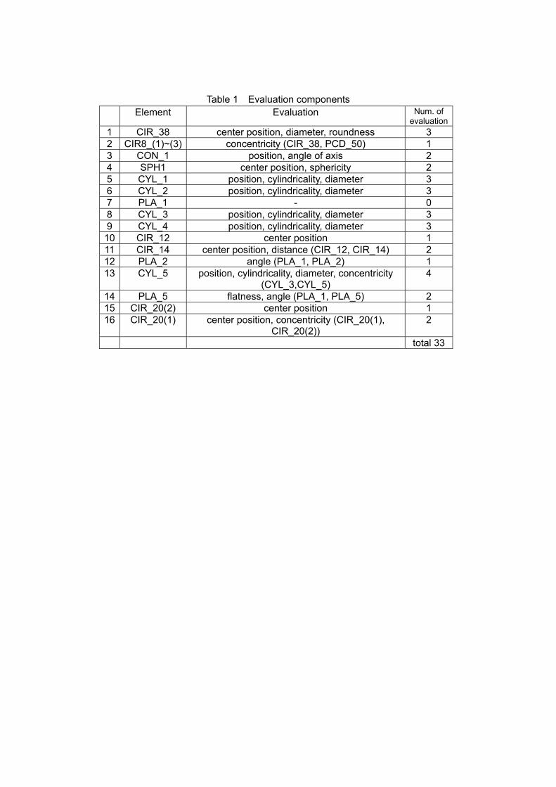
Table 1 Evaluation components Element Evaluation Num. of

evaluation 1 CIR_38 center position, diameter, roundness 3 2 CIR8_(1)~(3) concentricity (CIR_38, PCD_50) 1 3 CON_1 position, angle of axis 2 4 SPH1 center position, sphericity 2 5 CYL_1 position, cylindricality, diameter 3 6 CYL_2 position, cylindricality, diameter 3 7 PLA_1 - 0 8 CYL_3 position, cylindricality, diameter 3 9 CYL_4 position, cylindricality, diameter 3

10 CIR_12 center position 1 11 CIR_14 center position, distance (CIR_12, CIR_14) 2 12 PLA_2 angle (PLA_1, PLA_2) 1 13 CYL_5 position, cylindricality, diameter, concentricity

(CYL_3,CYL_5) 4

14 PLA_5 flatness, angle (PLA_1, PLA_5) 2 15 CIR_20(2) center position 1 16 CIR_20(1) center position, concentricity (CIR_20(1),

CIR_20(2)) 2

total 33


103

5.7 Activities on ISO/TC213/WG10

Ryoshu Furutani, Tokyo Denki University

1 Background of ISO/TC213 The homepage of ISO/TC213 says the scope and the task. 1.1 Scope Standardization in the field of geometrical product specifications (GPS) i.e. macro- and microgeometry specifications covering dimensional and geometrical tolerancing, surface properties and the related verification principles, measuring equipment and calibration requirements including the uncertainty of dimensional and geometrical measurements. The standardization includes the basic layout and explanation of drawing indications (symbols). 1.2 Task of ISO/TC213 Dimensioning and tolerancing leave a lot to be desired! I.e. the technical drawings are not unambiguous. Experience shows that the average costs involved amount to as much as 20% of the production turnover. The reason is not that the designer does not know what he or she wants, or that the workshop does not know how to comply with the drawing. The reason is lack of effective communication, resulting in misunderstanding from idea to the real thing. The poor communication arises from the fact that the parties do not know the "grammar" of the drawing and in particular from the fact that the available standards have not adequately kept pace with development. The technical drawing serves its purpose only if it is unique and results in the production of one single type of identical products with one single type of functional characteristics. The designer is responsible for ensuring that the technical drawing is unambiguous. The standardizers are responsible for ensuring that the designer has available to him the proper tools - namely the standards. There is an apparent need for improving the communication between the designer and the workshop. Several elements of the communication can be improved:


104

1. The human understanding and knowledge of the symbol language used on the drawing which expresses the functional characteristics of the workpiece by means of geometry. 2. Drawings shall be made more precise and unique which means that they shall specify all requirements that are essential for the function. 3. A complete, highly developed, systematic and standardized "language" is needed to express and translate the function of the workpiece into geometrical requirements on the drawing. Other geometrical characteristics, such as form, orientation, location and run-out and the macro and micro geometrical form characteristics of surfaces, are quite another story. These characteristics cannot be controlled during the process as they usually depend on parameters which cannot be controlled during the process. It is often the choice and order of the process and the material which have a decisive influence. Today the resulting deviations are relatively larger than the dimensional deviations, the difference being greater than before - the deviations are in fact so considerable that they obstruct the function of the workpiece as well as dimensioning and tolerancing. Deviations of form must consequently be limited to a higher degree than before by means of tolerances to ensure correct function of the workpiece and the relevance to dimensioning and tolerancing. The situation is that a marked shift has taken place between dimensional deviations and deviations of form, orientation, location and run-out. The problem is that the way of drawing and tolerancing has not changed. The ISO dimensioning and tolerancing system is based on the old ISA system which dates back to the 1940s, the ISO roughness system is from the 1950s. And because the ISO dimensioning and tolerancing system works only on theoretically correct workpieces - and not if deviations of form occur - the result is a drawing which does specify sufficiently precisely what is required of the geometry to obtain the desired function. As a consequence, far too much is left to the (random) decisions of other departments within the organization than the design/engineering department. It is therefore perfectly permissible to maintain the following: a) It is not the designer who decides the end function of the workpiece; b) It is the measuring and gauging people who decide the end function of the


105

workpiece by their (random) choice of measuring methods and equipment or the function is decided by the software integrated into the equipment; c) Where coincidence reigns, quality cannot be controlled; d) Subcontractors are at a loss. 1.3 Structure of ISO/TC213 ISO/TC213 had 11 Advisory Groups and 14 Working Groups. Some AG and WG had completed their missions and disbanded as shown in Table 1 and Figure 1.

Figure 1 Structure of ISO/TC213


106

Table 1 Advisory Groups and Working Groups of ISO/TC213

Advisory Groups Working Groups AG 1 Strategic planning

WG 1 Roundnes, Cylindricity, Straightness, Flatness

AG 2 Final auditing standards team

WG 2 Datums and datums systems

AG 3 Disbanded, transferred into WG 14

WG 3 Reference temperature


WG 4 Uncertaity

AG 5 Disbanded, work postponed

WG 5 Disbanded, task completed


WG 6 General requirements for GPS-measuring equipment


WG 7 ISO/DIS 2692

AG 8 Disbanded, transferred into AG 2

WG 8 Disbanded, task completed

AG 9 GPS-extraction techniques

WG 9 Dimensional and geometrical tolerancing for castings


WG 10 Coordinate measuring machines

AG 11 Underlying global concepts

WG 11 Disbanded, transferred into WG 6

WG 12 Size

WG 13 Disbanded

WG 14 Vertical GPS principles


107

2 Status ISO/TC213/WG10 have two major tasks. 1) ISO 10360-series:Acceptance and reverification tests for Coordinate Measuring

Machines 2) 2)ISO 15530-series: Techniques of Determining the Uncertainty of Measurement

in Coordinate Metrology The whole ISO 10360-Series were issued in 1999 and 2000. The parts of ISO 15530 are 15530-1: Terms 15530-2: Expert Judgment 15530-3: Substitution Method 15330-4: Simulation Method 15330-5: Historical Estimation 15530-6: Estimation using Uncalibrated objects. The 15530-3 will be issued as Technical Specifications as soon as Dr. Schwenke will give it some examples. The 15530-4 and -6 are now on the status of working draft. The project leader of the task force for ISO 15530-4 is Dr.Shakarji(NIST) and the members of the task force are Dr.Schwenke(PTB) and Prof.Takamasu(UT). We have had the task force meeting every WG10 and anual NEDO meeting in Tsukuba and Sydney since 1999. The concept of ISO 15530-4 have been presented every WG10 meeting since 1999. So, All experts from member bodies are familiar with the concept of simulation method. Most of them are considering ISO 15530-4 is similar test procedure to ISO 10360-6. The task force prepared following documents and had discussed, WG10N409 in Milan, in September 2000 WG10N424 in Bordeaux, in January 2001 WG10N454 in Madrid, in February 2002 N37-Annex-1(Our documents), in February 2002 Through the discussion of the task force meeting,

Test 1 and Test 2 were clearly distinguished. How to evaluate the simulation software, Test 1, is physical test.


108

We will plan the developing Test 1 first. 3 Future WG10 will have the meeting in September,2002 in Otawa and in January,2003 in Mexico. In both meeting, ISO 15530-4 will be presented according to the resolution in NEDO annual meeting in Sydney. We will continue to support Dr.Shakarji and make ISO 15530-4 be issued as soon as possible. Attached Documents:

ISO/TC 213/WG 10 N 409, Revision: September, 2000 Working Draft International Standard ISO/ 15530-4 Geometrical Product Specifications (GPS) - Techniques of Determining the Uncertainty of Measurement in Coordinate Metrology - Part 4: Estimating Task-Specific Measurement Uncertainty Using Simulation

ISO/TC 213/WG 10 N 424, Revision: January 2001

Working Draft International Standard ISO/ 15530-4 Geometrical Product Specifications (GPS) - Techniques of Determining the Uncertainty of Measurement in Coordinate Metrology - Part 4: Estimating Task-Specific Measurement Uncertainty Using Simulation

ISO/TC 213/WG 10 N 454, Revision: September 2001

Working Draft ISO/WD 15530-4 Geometrical Product Specifications (GPS) - Techniques of Determining the Uncertainty of Measurement in Coordinate Metrology - Part 4: Estimating Task-Specific Measurement Uncertainty Using Simulation

Some Conclusions at the NEDO Meeting in Sydney (1-Mar.-2002)

ISO/TC 213/WG 10 N 409 Revision: September, 2000 Note: This working draft is in an early form. Working Draft International Standard ISO/ 15530-4

Geometrical Product Specifications (GPS) - Techniques of Determining the Uncertainty of

Measurement in Coordinate Metrology - Part 4: Estimating Task-Specific Measurement Uncertainty

Using Simulation

Preliminary remark

For coordinate measuring machines (CMMs) used to control tolerances, the task-specific

uncertainties of measurement according to ISO 14253-1 must be taken into account when tests for

conformity/non-conformity are carried out. Knowledge of the uncertainty of measurement thus is of

utmost importance. Up to the present, there have been only a few procedures which allow the

task-specific uncertainty of measurement to be stated.

For simple measuring devices, this uncertainty can be estimated by an uncertainty budget

according to the recommendations of the Guide to the Expression of Uncertainty in Measurement

(GUM). However, in the case of CMM, the formulation of a classical uncertainty budget is,

impossible for the majority of the measurement tasks due to the complexity of the measuring

process.

Alternate methods can be used to determine the task-specific uncertainty of coordinate

measurements. One of them, which estimates the uncertainty by numerical simulation of the

measuring process allowing for uncertainty influences is described in the present standard.

1. Scope

It is the objective of the present standard to describe general conditions for the uncertainty

determination by simulation for specific measurement tasks carried out on CMMs, taking into

account the measuring device, the environment, the measurement strategy and the object. The

standard is to unify the general procedure without restricting the possibilities of the technical

realization. A procedure for verification and evaluation of the simulation package is included.

Measures are recommended which increase the procedure's transparency for the user, and

methods described which the user may apply to monitor it.

The sheet is not aimed at defining new parameters for the general evaluation of the accuracy of

measurement. The functional capability of the CMMs is taken for granted, agreement with

specifications is checked on the basis of sheets 1 - 6 of VDI 2617 and of the ISO series of

standards 10360.

2. Procedure

2.1 Principle

The functional principle is based on a computer-aided mathematical model of the measuring

process. In this model, the measuring process is represented from the measurand to the

measurement result, taking important influence quantities into account. In the simulation, these

influences are varied within their possible or assumed range of values (described by probability

distributions), and the measuring process is repeatedly simulated, using combinations of the

spectrum of all states considered possible. The uncertainty is determined from the variation of the

final result. This procedure is compatible with the fundamental principles of the internationally valid

Guide to the Expression of Uncertainty in Measurement (GUM).

2.2 Elements of the procedure

2.2.1 Uncertainty contributors

The measuring process on a CMM is subject to a great number of uncertainty contributors that

affect the measurement result. The following quantities (not complete) may contribute to the

uncertainty of the measurement result when measurements are carried out on a CMM:

• Geometry • Hysteresis • Long-term variation • Clamping

• Temperature • Dynamics • Specimen • ....

• Contacting system • Elasticity • Dirt

When the uncertainty of a measuring process is evaluated, these influence quantities must be

recognised and their effect on the measurement result described by a model.

2.2.2 Model

The model of the measuring process describes the mathematical relationship between the input

quantities (measurand and influence quantities) and the output measurement result. The

simulation procedure does not require that the model be described by a closed mathematical

expression. Numerical algorithms, such as the calculation of derived features or filtering of

measurement points can, therefore, be included in the model. This makes the simulation

procedure particularly suitable for complex measuring processes like coordinate measurements.

The model of the measurement on a CMM can be described by a signal flow chart, in which the

quantities influencing the measuring process are plotted. Figure 1 shows such a signal flow chart.

workpiece probing

strategy

geometry scales

evaluation

temperature

form errors

clamping

numr of points,

distribution,

prob.direction

geometric,

hystereses

dynamic effects

temp. gradients.

temperature

scale factor

non-linearities

algorithm,

precision

result

task

random errors

systematic

Figure 1: Measurement on a coordinate measuring machine represented in the form of a

signal flow chart

2.2.3 Simulator

With the aid of the simulator, all influence quantities are varied within their assumed probability

distribution and numerical calculation of the measurement result is repeatedly carried out. The

random values are generated in the assumed probability distributions by random number

generators which are to furnish approximately uncorrelated sequences of numbers.

2.2.4 Evaluation

By evaluation, the uncertainty of measurement is determined from the simulated measurement

results. The result of the evaluation of the simulation should be a statement in the form ±U which

describes the uncertainty range of the measurement result with a specified confidence level (cf.

also GUM).

2.3 Realisation

The simulation can be integrated into a control and evaluation software of a CMM (on-line) or

implemented as an independent system on an external computer (off-line). Both variants are

covered by this standard.

2.4 Limits of the procedure

The input quantities are estimated on the basis of best knowledge. The input quantities and their

uncertainties must, therefore, be well known. Usually, not all possible uncertainty influences are

taken into account in the model. Influence quantities which have not been considered are to be

estimated by other procedures and added to the total uncertainty.

3 Requirements and information to be provided by the manufacturer

3.1 Uncertainty contributors

The manufacturer of the simulation software must explicitly indicate which uncertainty contributors

(cf. 2.2.1) have been taken into account in his software and which information is required from the

user. In particular, the manufacturer should specify by means of this checklist, which uncertainty

contributors the software claims to take into account:

Influence Factors

CMM Types : � moving bridge � moving table � horizontal arm � gantry etc…

� Rotary Tables

CMM Errors: � static machine geometry errors � dynamic machine geometry errors � part loading effects � Non 20 C temperature � spatial gradients � temporal gradients � algorithm software accuracy � hysteresis Probe Types: � contact touch trigger � contact analog � non-contact optical Probe Errors: � probe response (lobing) � multiple styli � multiple probe � articulating head � styli/probe changing � scanning Nominal Parts: � circles � planes � sphere � cylinder � splines etc. GD&T: � datum ref frames � form � size � location � orientation Real Part Effects: � surface roughness � waviness � form error � non 20 C temp � spatial gradients � temporal gradients � contamination � fixturing Operator Effects: � sampling strategies, i.e. the number and location of points in the

workpiece coordinate system � workpiece position and orientation in machine coordinate system � other operator effects…

The manufacturer shall state what measurements or other quantities are needed to characterize

the CMM and its environment in order for the software to produce uncertainty statements (3.7).

The following contributors must at least be taken into account:

• The geometrical deviations of the CMM

• Deviations of the contacting system

• Influences of temporal and spatial temperature gradients on specimen and CMM

[Note: The details of which items should be on this list are yet to be determined]

3.2 Model

The model of the measuring process must take the most important principles of coordinate

measurement into account. Processing of the coordinates of the measurement points and

evalution of the geometrical quantities are to be modelled as integral parts of the measuring

process. The result must be a task-specific statement of the uncertainty for the final result of a

measurement.

The essential features of the model must be documented. Transparency of the model increases

the user's confidence in the statement of the uncertainty. Documentation of model and procedure

should be sufficient to enable the user to furnish proof of a statement of uncertainty in compliance

with the standards. This is important in particular in connection with the requirements of ISO 9000

foll. requiring the documentation of the procedure used for the uncertainty determination.

3.3 Simulator

The manufacturer shall describe how the influence quantities are varied. As a rule, the probability

distribution should be documented.

3.4 Statistical evaluation

The manufacturer must document how the uncertainties are derived from the simulated samples.

3.5 Statement of the uncertainty

It must be ensured that the statement of the uncertainty complies with the internationally valid

principles of the expression of the uncertainty (GUM). This includes the statement of a confidence

level or a coverage factor. The combined standard uncertainty may be indicated in addition to the

expanded uncertainty.

3.6 Operating conditions

Each factor “checked” in the declarations section (3.1) implies that the simulation software will

appropriately address this issue over a specified range of conditions. (For example, “non-standard

temperature” might be defined as homogenous temperature in space and time, within the limits of

15 °C to 30 °C.) The software manufacturer shall specify these ranges defining the spectrum of

measurement tasks and the environmental conditions for which the simulation is valid. Examples

of these ranges to be specified includes but is not limited to:

• Permissible part spectrum (e.g. exclusion of flexible sheet-metal parts, a minimum arc length for

circles, maximum cone apex angles, etc.)

• Permissible task spectrum (e.g. exclusion of scanning or form measurement)

• Permissible temperature range

• Permissible temporal temperature gradients dT/dt

• Permissible spatial temperature gradients dT/dx

• Other permissible environmental conditions

Within the scope of these restrictions, computer-aided verification and evaluation can be

performed, as well as the user checks, both described in section 5.

3.7 Input Quantities and How They Are Obtained

Along with the declarations described in section (3.1), the simulation software manufacturer must

specify in detail (or reference appropriate documents) what input quantities are required to

characterise the measurement system and how these quantities are obtained. These are the

values that are used by the simulation software to characterize the CMM, the environment,

operator effects etc. (Operator effects might be assessed from gauge repeatability and

reproducibility studies i.e., GR&R; analysis of variance, i.e. ANOVA; and from expert judgement,

i.e. "type B estimation").

4 Determination of the task-specific uncertainty of measurement The parameters of the simulated measurement which are important from the metrological point of

view should be as similar as possible to those of the real measurement. The standard uncertainty

of a measurement result y is composed of

- the uncertainty usim determined by the simulation, and

- the uncertainties ui from the influence quantities which have not be taken into account in

the simulation and have been manually estimated.

The combined standard uncertainty is then calculated with

∑+= 22isimges uuu . (1)

With the aid of coverage factors, this standard uncertainty can be brought to the desired

confidence level. As a rule, the following is valid

gesges uU ⋅= 2 (2)

for a confidence level of 95%. If the uncertainty stated by the simulation already is an expanded

uncertainty Usim, the simulated uncertainty usim is to be calculated by division with the respective

coverage factor.

5 Verification and Evaluation of Simulation Software

5.1 Principle The verification and evaluation of simulation software consists of two parts: A computer-aided

verification and evaluation procedure and a test using a physical object covering the whole system

composed of CMM, evaluation software and simulation software. The first is conducted only once

on a specific software release, while the latter is conducted multiple times on each software/CMM

combination.

5.2 Computer-Aided Verification and Evaluation (CVE)

This procedure uses computer simulation to verify and evaluate the simulation software. The

concept is to simulate a measuring instance, based on the claims in the declarations section (3.1).

Since the measuring instance is simulated and thus fully known in the CVE process, the error of

the simulated measurement can be found. The software under test produces an uncertainty

statement for this measurement and a simple comparison can determine if the error of the

simulated measurement was contained in the uncertainty region reported by the software under

test. This procedure can be repeated hundreds of times with varying conditions and statistics can

be determined regarding how often the errors of measurement were contained within their

corresponding reported uncertainty ranges.

5.2.1 Creation of a Simulated Measuring Instance used in CVE

When a CMM probes, there is generally a difference between the target contact point and the

measured point, this difference being a vector. So a simulated measuring instance can be created

by defining a vector field over the measuring volume of the CMM. That is, associated with each

point in the CMM’s measuring volume is a vector that represents the difference between the target

contact point and the simulated measured point.

For the purposes of CVE, the declarations section (3.1) determines what influences the

definition of the vector field. For instance, if hysterisis is claimed in section (3.1) then the vector

associated with a particular point on one query would, in general, be different than on a

subsequent query. If part form errors are included in the declarations section (3.1) then the vector

associated with a particular point would depend on the placement of the part in the measuring

volume. This allows for testing the software’s reported uncertainties without combining them with

other uncertainties.

5.2.2 Creation of Input Quantities

The declarations section includes the indication of the input quantities required by the software

(3.1, 3.7). These input quantities might arise from probes of special calibrated workpieces.

Appropriate input quantities can be obtained as follows: A simulated measuring instance can be

created in accordance with the specifications of the manner in which input quantities are obtained

(3.1, 3.7). Note, these conditions might be different than the ranges given in the checklist (e.g. the

input quantities might be measured close to 20°C, while the software allows for measurements

over a wider temperature range.) The target contact points used in the procedure to determine

input quantities are provided to the testing body and the testing body returns the corresponding

measured contact points from the simulated measuring instance. The software under test must be

able to exchange this information.

5.2.3 CVE Testing

The CVE testing proceeds as shown in the following diagram given as a illustrative example using

point-to-point length measurements:

CMM Population

Create U Statement

Calculate Pt-PtLength Error

Perform CMM Assessment

Create Pt-Pt Length

Compare: |E| < U ?

Select One CMM

Are 95% of Lengths Successful?

Success Statistics

Yes = “successful” No = “unsuccessful”

Repeat process with new length

Pass / Fail Statistics

Yes = “Pass” this CMM No = “Fail” this CMM

Report % CMMs Pass & Lengths Successful

Repeat process with new CMM

5.2.4 Reporting CVE Results

CVE results consist of the following information:

• The percent of time true value lies in uncertainty interval; e.g. for "good" software the threshold

might be 95%.

• The average amount of over-estimation of uncertainty, i.e. when the true value is contained

within the uncertainty interval, on average how far is it from the nearest uncertainty interval

limit.

• The average amount of under-estimation of uncertainty, i.e. when the true value is outside the

uncertainty interval, on average how far is it from the nearest uncertainty interval limit.

5.3 Verification Using a Calibrated Workpiece

In addition to the CVE, this procedure provides verification for a specific task for a specific

software/CMM combination. Here, the statement of the uncertainty is checked by a test covering

the whole system composed of CMM, evaluation software, and simulation software. The test is

based on real measurements performed on calibrated objects. Each object permitted according to

section 3.5 may be used. The object must have been calibrated by an independent procedure. In

the Annex, an object and a procedure are given as an example, and show a number of

measurement tasks to be simulated and which can also be calibrated with sufficient accuracy by

independent procedures. For the measurement of such an object it is recommended to vary also

the measurement strategy (position and orientation of the test object, distribution of measurement

points) in order to check the influence on the measurement uncertainty stated.

The following test objects may also be used: gauge blocks, step gauges, ball plates and other

standards. However any specific object is only suited to a limited extent to test the statements of

task-specific uncertainty.

5.3.1 Procedure

The measurements on the calibrated test objects are carried out on the real CMM for which the

uncertainty of measurement is to be determined. The real measurement results y are calculated

and the related task-specific uncertainties of measurement Uges determined by simulation.

5.3.2 Calculation of the test result

Performing a number of measurements on calibrated objects, the coverage of the uncertainty

ranges is checked. A statement of uncertainty will be plausible if:

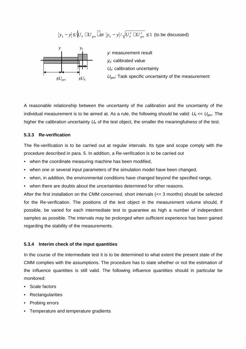
( )geskk UUyy +≤− or 1/ 22 ≤+− geskk UUyy (to be discussed)

y yk

±Uk±Uges

y: measurement result

yk: calibrated value

Uk: calibration uncertainty

Uges: Task specific uncertainty of the measurement

A reasonable relationship between the uncertainty of the calibration and the uncertainty of the

individual measurement is to be aimed at. As a rule, the following should be valid: UK << Uges. The

higher the calibration uncertainty UK of the test object, the smaller the meaningfulness of the test.

5.3.3 Re-verification The Re-verification is to be carried out at regular intervals. Its type and scope comply with the

procedure described in para. 5. In addition, a Re-verification is to be carried out

• when the coordinate measuring machine has been modified,

• when one or several input parameters of the simulation model have been changed,

• when, in addition, the environmental conditions have changed beyond the specified range,

• when there are doubts about the uncertainties determined for other reasons.

After the first installation on the CMM concerned, short intervals (<= 3 months) should be selected

for the Re-verification. The positions of the test object in the measurement volume should, if

possible, be varied for each intermediate test to guarantee as high a number of independent

samples as possible. The intervals may be prolonged when sufficient experience has been gained

regarding the stability of the measurements.

5.3.4 Interim check of the input quantities In the course of the intermediate test it is to be determined to what extent the present state of the

CMM complies with the assumptions. The procedure has to state whether or not the estimation of

the influence quantities is still valid. The following influence quantities should in particular be

monitored:

• Scale factors

• Rectangularities

• Probing errors

• Temperature and temperature gradients

The input quantities should preferably be monitored by the procedures usually applied in

coordinate measurement technology.

Annex

l

A Br B

Ac

d

b b

Figure A-1: Test cylinder for verification of the simulation

Symbol Brief description of the feature

I Distance of end faces

d Diameter of a cylinder

r Rectangularity deviations of the end faces with respect to a cylinder axis

c Coaxiality of the cylinder axes

(b) Reference length for the measurement of coaxiality and rectangularity according to ISO 1101 (no feature)

1

3 4

2

B CA

x

z

y

Figure A-2: Positions of the test cylinder in the measurement volume and probe configurations.

ISO/TC 213/WG 10 N 424 Revision: January 2001 Working Draft International Standard ISO/ 15530-4



Using Simulation

Preliminary remark

For coordinate measuring machines (CMMs) used to control tolerances, the task-specific


conformity/non-conformity are carried out. Knowledge of the uncertainty of measurement thus is of

utmost importance. Up to the present, there have been only a few procedures which allow the

task-specific uncertainty of measurement to be stated.

For simple measuring devices, this uncertainty can be estimated by an uncertainty budget


(GUM). However, in the case of CMM, the formulation of a classical uncertainty budget is,


process.

Alternate methods can be used to determine the task-specific uncertainty of coordinate

measurements. One of them, which estimates the uncertainty by numerical simulation of the

measuring process allowing for uncertainty influences is described in the present standard.

1. Scope

It is the objective of the present standard to describe general conditions for the uncertainty

determination by simulation for specific measurement tasks carried out on CMMs, taking into

account the measuring device, the environment, the measurement strategy and the object. The

standard is to unify the general procedure without restricting the possibilities of the technical

realization. A procedure for verification and evaluation of the simulation package is included.

Measures are recommended which increase the procedure's transparency for the user, and

methods described which the user may apply to monitor it.

The sheet is not aimed at defining new parameters for the general evaluation of the accuracy of

measurement. The functional capability of the CMMs is taken for granted, agreement with

specifications is checked on the basis of sheets 1 - 6 of VDI 2617 and of the ISO series of

standards 10360.

2. Procedure

2.1 Principle

The functional principle is based on a computer-aided mathematical model of the measuring

process. In this model, the measuring process is represented from the measurand to the

measurement result, taking important influence quantities into account. In the simulation, these

influences are varied within their possible or assumed range of values (described by probability

distributions), and the measuring process is repeatedly simulated, using combinations of the

spectrum of all states considered possible. The uncertainty is determined from the variation of the

final result. This procedure is compatible with the fundamental principles of the internationally valid

Guide to the Expression of Uncertainty in Measurement (GUM).

2.2 Elements of the procedure

2.2.1 Uncertainty contributors

The measuring process on a CMM is subject to a great number of uncertainty contributors

(Section 3.1) that affect the measurement result. When the uncertainty of a measuring process is

evaluated, these influence quantities must be accounted for, recognizing that, in general, the

simulator accounts for only some of these influence quantities.

2.2.2 Model

The model of the measuring process describes the mathematical relationship between the input

quantities (measurand and influence quantities) and the output measurement result. The

simulation procedure does not require that the model be described by a closed mathematical

expression. Numerical algorithms, such as the calculation of derived features or filtering of

measurement points can, therefore, be included in the model. This makes the simulation

procedure particularly suitable for complex measuring processes like coordinate measurements.

The model of the measurement on a CMM can be described by a signal flow chart, in which the

quantities influencing the measuring process are plotted. Figure 1 shows such a signal flow chart.

workpiece probing

strategy

geometry scales

evaluation

temperature

form errors

clamping

numr of points,

distribution,

prob.direction

geometric,

hystereses

dynamic effects

temp. gradients.

temperature

scale factor

non-linearities

algorithm,

precision

result

task

random errors

systematic


signal flow chart

2.2.3 Simulator

With the aid of the simulator, all influence quantities (within its scope) are varied within their

assumed probability distribution and numerical calculation of the measurement result is repeatedly

carried out. The random values are generated in the assumed probability distributions by random

number generators which are to furnish approximately uncorrelated sequences of numbers.

2.2.4 Evaluation

By evaluation, the uncertainty of measurement is determined from the simulated measurement

results. The result of the evaluation of the simulation should be a statement in the form ±U which

describes the uncertainty range of the measurement result with a specified confidence level (cf.

also GUM).

2.3 Realisation

The simulation can be integrated into a control and evaluation software of a CMM (on-line) or



2.4 Limits of the procedure

The input quantities are estimated on the basis of best knowledge. The input quantities and their

uncertainties must, therefore, be well known. Usually, not all possible uncertainty influences are

taken into account in the model. Influence quantities which have not been considered are to be

estimated by other procedures and added to the total uncertainty.

3 Requirements and information to be provided by the manufacturer

3.1 Uncertainty contributors

The manufacturer of the simulation software must explicitly indicate which uncertainty contributors

(cf. 2.2.1) have been taken into account in the software and which information is required from the

user. In particular, the manufacturer should specify by means of this checklist, which uncertainty


Influence Factors


� Rotary Tables




the CMM and its environment in order for the software to produce uncertainty statements (3.7).






3.2 Model

The model of the measuring process must take the most important principles of coordinate

measurement into account. Processing of the coordinates of the measurement points and

evaluation of the geometrical quantities are to be modelled as integral parts of the measuring

process. The result must be a task-specific statement of the uncertainty for the final result of a

measurement.

The essential features of the model must be documented. Transparency of the model increases

the user's confidence in the statement of the uncertainty. Documentation of model and procedure

should be sufficient to enable the user to furnish proof of a statement of uncertainty in compliance

with the standards. This is important in particular in connection with the requirements of ISO 9000

foll. requiring the documentation of the procedure used for the uncertainty determination.

3.3 Simulator

The manufacturer shall describe how the influence quantities are varied. As a rule, the probability

distribution should be documented.

3.4 Statistical evaluation

The manufacturer must document how the uncertainties are derived from the simulated samples.

3.5 Statement of the uncertainty

It must be ensured that the statement of the uncertainty complies with the internationally valid

principles of the expression of the uncertainty (GUM). This includes the statement of a confidence

level or a coverage factor. The combined standard uncertainty may be indicated in addition to the

expanded uncertainty.

3.6 Operating conditions

Each factor “checked” in the declarations section (3.1) implies that the simulation software will















3.7 Input Quantities and How They Are Obtained

Along with the declarations described in section (3.1), the simulation software manufacturer must







4 Determination of the task-specific uncertainty of measurement The parameters of the simulated measurement which are important from the metrological point of





the simulation and have been estimated by other appropriate means.


∑+= 22isimges uuu . (1)






coverage factor.

5 Verification and Evaluation of Simulation Software

5.1 Principle The verification and evaluation of simulation software consists of two parts: TEST 1: A thorough,

general software test covering a wide range of capabilities of the simulation software, and TEST 2:

a test using a physical object on a specific implementation of the software on a particular CMM

and covering the whole system composed of CMM, evaluation software, and simulation software.

TEST 1 is conducted only once on a specific software release, while TEST 2 is conducted multiple

times on each software/CMM combination.

TEST 1 • Performed only once for a given release of the software. • Performed by software supplier along with testing bodies. • Rigorous test covering many measurands • Can be done using either computer-aided verification and

evaluation or by extensive physical testing

TEST 2 Performed by the user in conjunction with a particular CMM

Software distribution



TEST 2 • Performed for every combination of software and CMM • Performed by user without the need for a testing body • Faster, easier, and not as exhaustive as TEST 1 • Must be done using physical testing

5.2 TEST 1

(DRAFT NOTE: Currently this standard only describes the computer-aided verification and

evaluation (CVE) for test 1. An alternate means for achieving TEST 1 by using extensive physical

measurements is being investigated.)










5.2.1 Creation of a Simulated Measuring Instance used in CVE

When a CMM probes, there is generally a difference between the target contact point and the






definition of the vector field. For instance, if hysteresis is claimed in section (3.1) then the vector






5.2.2 Creation of Input Quantities

The declarations section includes the indication of the input quantities required by the software










5.2.3 CVE Testing

The CVE testing should be performed over the entire spectrum of measurands for which the

software is claimed to be valid. The CVE testing proceeds as shown in the following diagram given

as a illustrative example using point-to-point length measurements:

5.2.4 Reporting CVE Results

CVE results consist of the following information:


might be 95%.



limit.



CMM Population

Create U Statement

Calculate Pt-PtLength Error

Perform CMM Assessment

Create Pt-Pt Length

Compare: |E| < U ?

Select One CMM

Are 95% of Lengths Successful?

Success Statistics







5.3 Verification Using a Calibrated Workpiece

In addition to the CVE, this procedure provides verification for a specific task for a specific



based on real measurements performed on calibrated objects. Any object permitted according to




independent procedures. For the measurement of such an object it is recommended to also vary



The following test objects may also be used: gauge blocks, step gauges, ball plates, ball bars and

other standards. However any specific object is only suited to a limited extent to test the

statements of task-specific uncertainty.

5.3.1 Procedure



and the related task-specific uncertainties of measurement Uges are determined by simulation.

5.3.2 Calculation of the test result

Performing a number of measurements on calibrated objects, the coverage of the uncertainty


1/ 22 ≤+− geskk UUyy

y yk

±Uk±Uges








5.3.3 Re-verification

The Re-verification is to be carried out at regular intervals. Its type and scope comply with the











5.3.4 Interim check of the input quantities In the course of the intermediate test it is to be determined to what extent the present state of the



monitored:

• Scale factors


• Probing errors




Annex

l

A Br B

Ac

d

b b




d Diameter of a cylinder

r Rectangularity deviations of the end faces with respect to a cylinder axis

c Coaxiality of the cylinder axes


1

3 4

2

B CA

x

z

y


1

ISO/TC 213/WG 10 N 454 Revision: September 2001 Working Draft ISO/WD 15530-4



Using Simulation

Preliminary remark

For coordinate measuring machines (CMMs) used to inspect tolerances, the task-specific


conformity/non-conformity are carried out. Thus knowledge of the uncertainty of measurement is of

utmost importance. Up to the present, there have been only a few procedures that allow the task-

specific uncertainty of measurement to be stated.

For simple measuring devices this uncertainty can be estimated by an uncertainty budget


(GUM). However, in the case of a CMM, the formulation of a classical uncertainty budget is


process.

Alternate methods that are consistent with the GUM can be used to determine the task-specific

uncertainty of coordinate measurements. One of them, which estimates the uncertainty by

numerical simulation of the measuring process allowing for uncertainty influences, is described in

this standard.

1. Scope It is the objective of this standard to describe testing procedures for the evaluation of task specific

uncertainty determination by simulation for specific measurement tasks carried out on CMMs,

taking into account the measuring device, the environment, the measurement strategy and the

object. The standard is to unify the general procedures without restricting the possibilities of the

technical realization. A procedure for verification and evaluation of the simulation package is

included. Measures are recommended that increase the procedure's transparency for the user,

and methods are described that the user may apply to monitor it.

The standard is not aimed at defining new parameters for the general evaluation of the

accuracy of CMM measurements. The functional capability of the CMMs is taken for granted, as

agreement with specifications is checked on the basis of sheets 1 - 6 of VDI 2617 and of the ISO

series of standards 10360.

2

2. Terminology: (To be defined; descriptions are given when used first) Influence Quantity

Input Quantity

Uncertainty Evaluating Software (UES)

Uncertainty Evaluating Software Evaluation (UESE)

Uncertainty Evaluating Software Implementation Test (UESIT)

Computer-aided Verification and Evaluation (CVE)

3. Overview The generation of task specific uncertainty statements for CMM measurements is a complex

issue. To allow CMM users to easily create uncertainty statements, CMM suppliers and other third

party companies have developed Uncertainty Evaluating Software (UES). UES is based on a

computer-aided mathematical model of the measuring process. In this model, the measuring

process is represented from the measurand to the measurement result, taking important influence

quantities into account. In the simulation, these influences are varied within their possible or

assumed range of values (described by probability distributions), and the measuring process is

repeatedly simulated, using possible combinations of the influence quantities. The uncertainty is

determined from the variation of the final result. This procedure is compatible with the fundamental

principles of the internationally valid Guide to the Expression of Uncertainty in Measurement

(GUM). The details of the UES are often hidden in complied computer code making it difficult for

the user to assess the reliability of the calculated uncertainty statements. This standard sets forth

terminology and testing procedures for both the UES supplier and the CMM user to communicate

and quantify the capability of UES.

This standard divides the problem into three major parts. The first part (section 4) is the

declaration of influence quantities. The declarations identify which influence quantities, along with

their ranges of values, the UES can account for in its uncertainty evaluation. For example, some

UES can include the effects of using multiple styli during a CMM measurement, while others

cannot. Similarly, some UES can include the effects of temporal or spatial temperature gradients,

while others cannot. The purpose of the declaration section is to clearly identify to the CMM user

what influence quantities, and their ranges of values, the UES will consider in its uncertainty

evaluation. This will allow the user to be able to make informed decisions. Purchasing a UES

product with limited capabilities that do not include some influence quantities present during the

CMM measurements requires the CMM user to independently evaluate these unaccounted-for

influence quantities and combine them appropriately with those that are evaluated by the UES in

order to produce a GUM compliant uncertainty statement.

3

The second part describes the testing procedure for the uncertainty evaluating software evaluation

(UESE). The UESE is performed by a testing body and is only conducted once for each version of

the UES. The UESE is a major evaluation that tests the UES for its ability to produce appropriate

uncertainty statements under any combination of influence quantities permitted in the declaration

section.

The third part describes the final test which is performed by the CMM user on a particular CMM.

This Uncertainty Evaluating Software Implementation Test (UESIT) checks that the UES and its

associated input values are correctly installed and working properly. The UESIT may also detect a

large uncertainty source that is not taken into account by the UES but is present in the CMM

system.

4.0 Elements of the UES The simulation can be integrated into a control and evaluation software of a CMM (on-line) or



4.1 Uncertainty Contributors

The measuring process of a CMM is subject to a great number of uncertainty contributors

(influence quantities) that affect the measurement result. When the uncertainty of a measuring

process is evaluated using the UES, these influence quantities must be accounted for, recognizing

that, in general, the UES accounts for only some of these influence quantities.

4.2 UES Model The model of the measuring process employed by the UES describes the mathematical

relationship between the input quantities (measurand and influence quantities) and the output

measurement result. The UES does not require that the model be described by a closed

mathematical expression. Numerical algorithms, such as the calculation of derived features or

filtering of measurement points can, therefore, be included in the model. This makes UES

particularly suitable for complex measuring processes like coordinate measurements. The model

used by UES of the measurement on a CMM can be described by a flow chart, in which the

quantities influencing the measuring process are plotted. Figure 1 shows a typical flow chart.

4

workpiece probing

strategy

geometry scales

evaluation

temperatureform errorsclamping

numr of points,distribution,

prob.direction

geometric,hystereses

dynamic effectstemp. gradients.

temperaturescale factor

non-linearities

algorithm,precision

result

task

random errors

systematic


flow chart

Usually, not all possible uncertainty influences are taken into account in the model. Influence

quantities which have not been considered are to be estimated by other procedures and added to

the total uncertainty as follows: 4.3 Determination of the task-specific uncertainty of measurement The parameters of the simulated measurement which are important from the metrological point of





the simulation and have been estimated by other appropriate means.


�+= 22isimges uuu . (1)






coverage factor.

5

4.4 Requirements and information to be provided by the manufacturer 4.4.1 Influence Quantities The manufacturer of the UES shall explicitly declare which influence quantities (cf. 2.2.1) have

been taken into account in the software, and what information is required from the user. In

particular, the manufacturer should specify by means of this checklist, which uncertainty


Declaration of Influence Quantities


� Rotary Tables




the CMM and its environment in order for the UES to produce uncertainty statements (3.7).






4.4.2 Operating conditions Each factor “checked” in the declarations section (3.1) implies that the simulation software will



6













4.4.3 Input Quantities and How They Are Obtained Along with the declarations described in section (3.1), the simulation software manufacturer must







4.4.4 Additional UES Requirements • The manufacturer shall describe how the influence quantities are varied. As a rule, the

probability distribution should be documented.

• The manufacturer must document how the uncertainties are derived from the simulated

samples.

• The essential features of the model must be documented. Transparency of the model

increases the user's confidence in the statement of the uncertainty. Documentation of model

and procedure should be sufficient to enable the user to furnish proof of a statement of

uncertainty in compliance with the standards. This is important in particular in connection with

the requirements of ISO 9000 foll. requiring the documentation of the procedure used for the

uncertainty determination.

• The result of the evaluation of the simulation should be a statement in the form ±U which

describes the uncertainty range of the measurement result with a specified confidence level

(cf. also GUM).

• It must be ensured that the statement of the uncertainty complies with the internationally valid

principles of the expression of the uncertainty (GUM). This includes the statement of a

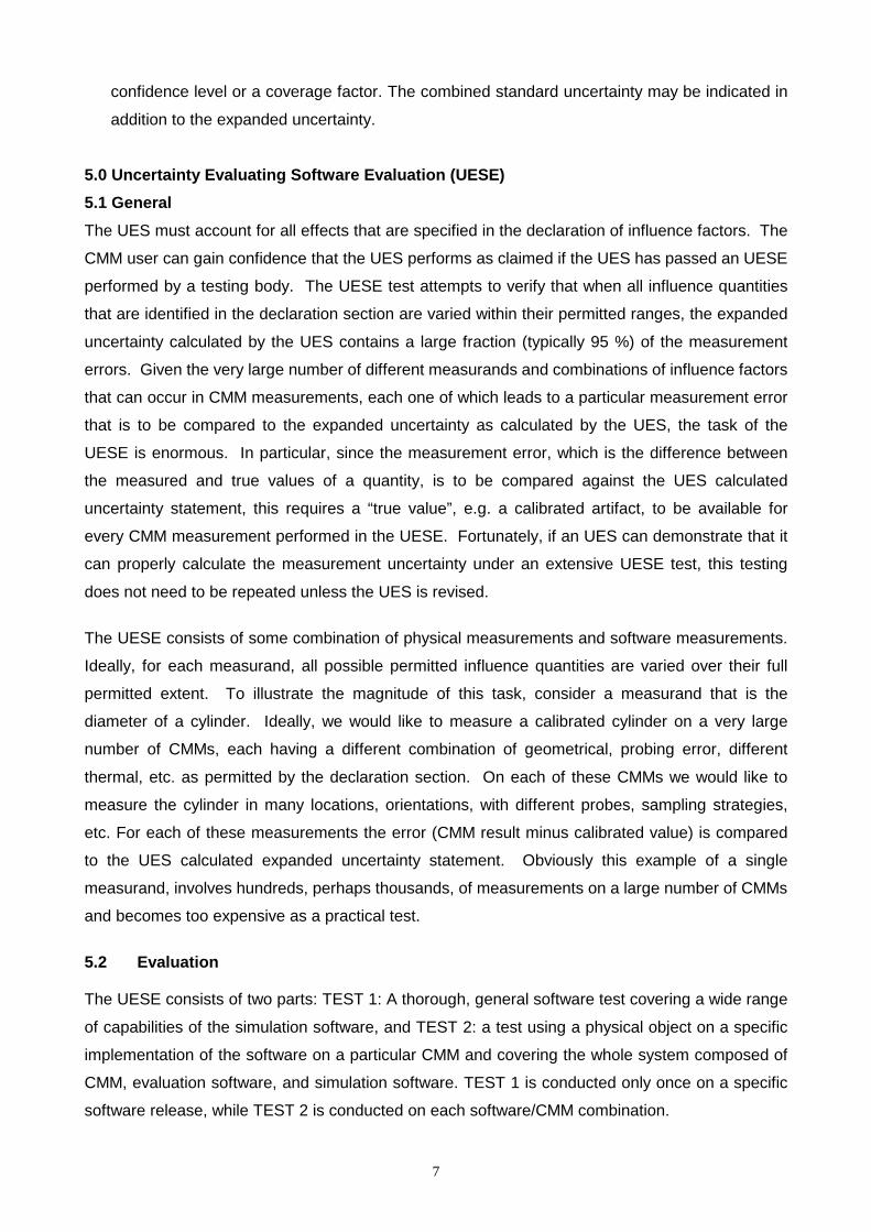
7

confidence level or a coverage factor. The combined standard uncertainty may be indicated in

addition to the expanded uncertainty.

5.0 Uncertainty Evaluating Software Evaluation (UESE) 5.1 General The UES must account for all effects that are specified in the declaration of influence factors. The

CMM user can gain confidence that the UES performs as claimed if the UES has passed an UESE

performed by a testing body. The UESE test attempts to verify that when all influence quantities

that are identified in the declaration section are varied within their permitted ranges, the expanded

uncertainty calculated by the UES contains a large fraction (typically 95 %) of the measurement

errors. Given the very large number of different measurands and combinations of influence factors

that can occur in CMM measurements, each one of which leads to a particular measurement error

that is to be compared to the expanded uncertainty as calculated by the UES, the task of the

UESE is enormous. In particular, since the measurement error, which is the difference between

the measured and true values of a quantity, is to be compared against the UES calculated

uncertainty statement, this requires a “true value”, e.g. a calibrated artifact, to be available for

every CMM measurement performed in the UESE. Fortunately, if an UES can demonstrate that it

can properly calculate the measurement uncertainty under an extensive UESE test, this testing

does not need to be repeated unless the UES is revised.

The UESE consists of some combination of physical measurements and software measurements.

Ideally, for each measurand, all possible permitted influence quantities are varied over their full

permitted extent. To illustrate the magnitude of this task, consider a measurand that is the

diameter of a cylinder. Ideally, we would like to measure a calibrated cylinder on a very large

number of CMMs, each having a different combination of geometrical, probing error, different

thermal, etc. as permitted by the declaration section. On each of these CMMs we would like to

measure the cylinder in many locations, orientations, with different probes, sampling strategies,

etc. For each of these measurements the error (CMM result minus calibrated value) is compared

to the UES calculated expanded uncertainty statement. Obviously this example of a single

measurand, involves hundreds, perhaps thousands, of measurements on a large number of CMMs

and becomes too expensive as a practical test.

5.2 Evaluation The UESE consists of two parts: TEST 1: A thorough, general software test covering a wide range

of capabilities of the simulation software, and TEST 2: a test using a physical object on a specific

implementation of the software on a particular CMM and covering the whole system composed of

CMM, evaluation software, and simulation software. TEST 1 is conducted only once on a specific

software release, while TEST 2 is conducted on each software/CMM combination.

8

5.2.1 TEST 1 (DRAFT NOTE: Currently this standard briefly describes only the computer-aided verification and

evaluation (CVE) for test 1. An alternate means for achieving TEST 1 by using extensive physical

measurements is being investigated.)










5.2.1.1 Creation of a Simulated Measuring Instance used in CVE When a CMM probes, there is generally a difference between the target contact point and the



TEST 1 • Performed only once for a given release of the software. • Performed by software supplier along with testing bodies. • Rigorous test covering many measurands • Can be done using either computer-aided verification and

evaluation or by extensive physical testing

TEST 2 Performed by the user in conjunction with CMM-1

Software distribution



TEST 2 • Performed for every combination of software and CMM • Performed by user without the need for a testing body • Faster, easier, and not as exhaustive as TEST 1 • Must be done using physical testing

9




definition of the vector field. For instance, if hysteresis is claimed in section (3.1) then the vector






5.2.1.2 Creation of Input Quantities The declarations section includes the indication of the input quantities required by the software










5.2.1.3 CVE Testing The CVE testing should be performed over the entire spectrum of measurands for which the

software is claimed to be valid. The CVE testing proceeds as shown in the following diagram:

10

5.2.1.4 Reporting CVE Results CVE results consist of the following information:


might be 95%.



limit.



5.2.2 Verification Using a Calibrated Workpiece In addition to the CVE, this procedure provides verification for a specific task for a specific



based on real measurements performed on calibrated objects. Any object permitted according to




independent procedures. For the measurement of such an object it is recommended to also vary

CMM Population

Create U Statement

Calculate Meas. Error

Perform CMMAssessment

Create Measurement

Compare: |E| < U ?

Select One CMM

Are 95% of Meas. Successful?

Success Statistics







11



The following test objects may also be used: gauge blocks, step gauges, ball plates, ball bars and

other standards. However any specific object is only suited to a limited extent to test the

statements of task-specific uncertainty.

5.2.2.1 Procedure



and the related task-specific uncertainties of measurement Uges are determined by simulation.

5.2.2.2 Calculation of the test result Performing a number of measurements on calibrated objects, the coverage of the uncertainty


1/ 22 ≤+− geskk UUyy

y yk

±Uk±Uges








5.2.2.3 Re-verification The Re-verification is to be carried out at regular intervals. Its type and scope comply with the











12

5.2.2.4 Interim check of the input quantities In the course of the intermediate test it is to be determined to what extent the present state of the



monitored:

• Scale factors


• Probing errors




13

Annex

l

A Br B

Ac

d

b b




D Diameter of a cylinder

R Rectangularity deviations of the end faces with respect to a cylinder axis

C Coaxiality of the cylinder axes


1

3 4

2

B CA

x

z

y


International Joint Research Grant Nedo-VCMM team

NEDO-VCMM N37 - 1

We agree on the general concept of the 15530-4 standard, seeing the main open question is that of the details of Test 1. We also agreed that publication of the standard should not be needlessly delayed. Test 1 can and should be useful for increasing confidence in uncertainty evaluating software. Still open for Test 1 are issues of the use of software testing, hardware testing, or a combination of these two (possible by using the decomposition method) We agreed that we would proceed with physical testing for Test 1 unless we find ourselves compelled to look to computer aided evaluation. We plan to proceed with developing a Test 1 type procedure for evaluating the ability of the software under test to reflect various sampling strategies using physical testing. This should serve as a starting example. We will try to incorporate this procedure, along with other modifications into a new 15530-4 draft for the next WG 10 meeting. Currently we will proceed with the thought that Test 1 would be performed by an NMI. Thus the test designed should reflect the resources and possibilities of an NMI unless we are compelled to consider possibilities beyond NMIs. The 15530-4 task force would like to thank the attendees of this NEDO meeting for their excellent and kind input.

NEDO-VCMM team

Virtual Coordinate Measuring Machine

NEDO-VCMM N37-Annex-1

25-Feb-2002

Some Conclusions at the NEDO Meeting in Sydney (1-Mar.-2002)

NEDO VCMM-Team: 6. Publication List

147

6. Publication List

6.1 Publication List by The University of Tokyo (pp. 160 - 303)

Journal Papers

1) Kiyoshi Takamasu, Ryoshu Furutani, Shigeo Ozono: Basic Concept of Feature-Based Metrology, Measurement, 26 (3), 1999, pp. 151-156.

2) 阿部誠，高増潔，大園成夫，沢辺雅二：空間座標の比較測定による CMM の

構成（第 1 報）－パラメトリックエラーモデルの構成とそのシミュレーショ

ン－，精密工学会誌，66（3），2000，pp. 483-488．

3) 高増潔，阿部誠，古谷涼秋，大園成夫：形体計測における不確かさの見積り

（第 1 報）－校正作業で生じる系統誤差の寄与－，精密工学会誌，67（1），2001，pp. 91-95

4) 阿部誠，高増潔，大園成夫：空間座標の比較測定による CMM の校正（第 2報）－パラメトリックエラー推定値の信頼性－，精密工学会誌，66（4），2000，pp. 578-582

5) G.Olea, N. Plitea, K. Takamasu: Kinematical Analysis and Simulation of a New Parallel Mechanism for Robotics’ Application, Advances in Robot Kinematics, Kluwer Academic Publishers, 2000, pp. 403-410

6) 阿部誠，高増潔，大園成夫：座標比較による CMM 校正システムの開発（第 1報）－試作システムの構成とその基本的な評価－，精密工学会誌，67（4），2001，638-643

7) 阿部誠，高増潔，大園成夫：座標比較による CMM 校正システムの開発（第 2報）－校正の信頼性の統計的な評価－，精密工学会誌，67（6），2001，976-981

8) M. Fujiwara, A. Yamaguchi, K. Takamasu and S. Ozono: Evaluation of Stages of Nano-CMM, Initiatives of precision engineering at the beginning of a millennium (edited by Ichiro Inasaki), Kluwer Academic Publishers (Netherlands), 2001, 634-638

9) Sato, M. Hiraki, K. Takamasu and S. Ozono: Calibration of 2-DOF Parallel Mechanism, Initiatives of precision engineering at the beginning of a millennium (edited by Ichiro Inasaki), Kluwer Academic Publishers (Netherlands), 2001, 734-738


148

Proceedings (International Conference)

1) Kiyoshi Takamasu, Masahiko Hiraki, Kazuhiro Enami, Shigeo Ozono: Development of Nano-CMM and Parallel-CMM - CMM in the 21th Century -, Int. Dimensional Metrology Workshop, 1999.

2) K. Takamasu, R. Furutani, S. Ozono: Statistical Evaluation of Minimum Zone Method in Coordinate Metrology, IMEKO-XV World Congress, 1999, pp. 101-106.

3) M. Hiraki, N. Yoshikawa, K. Takamasu, S. Ozono: Development of 3 DOF Parallel-CMM, IMEKO-XV World Congress, 1999, pp. 123-128.

4) K. Takamasu, M. Fujiwara, H. Naoi, S. Ozono: Friction Drive System for Nano-CMM, Proc. Mechatronics 2000, 2000, pp. 565-568

5) M. Abbe, K. Takamasu, S. Ozono: Reliability of Parametric Error on Calibration of CMM, IMEKO-XVI World Congress, 2000, pp. 180-184

6) G. Olea, M. Hiraki, K. Takamasu, S. Ozono: Kinematics Analysis, Simulation and Design of a Parallel Mechanism with R-L Actuators, Proc. Parallel Kinematic Machines Int. Conf. 2000, 2000, pp. 297-305

7) K. Takamasu, M. Fujiwara, A. Yamaguchi, M. Hiraki and S. Ozono: Evaluation of Thermal Drift of Nano-CMM, Euspen2001（トリノ，2001 年 5 月）, 2001, 306-309

8) K. TAKAMASU, M. ABBE, R. FURUTANI and S. OZONO: Estimation of Uncertainty in Feature-Based Metrology, ISMTII2001（エジプト，2001 年 9 月）, 2001, 47-52

Proceedings (Domestic Conference)

1) 佐藤理，平木雅彦，高増潔，大園成夫，吉川暢広：パラレルメカニズムを用

いた三次元測定機の研究（第 9 報）－リニアスケールの搭載－，1999 年度精

密工学会秋季大会学術講演会講演論文集，1999，p. 346．

2) 高増潔：座標測定における計測の不確かさ，1999 年度精密工学会秋季大会学

術講演会講演論文集，1999，p. 438．

3) 阿部誠，高増潔，大園成夫：CMM 校正の不確かさに関する 1 考察（第 1 報）

－1 次元変位測定によるパラメトリックエラー推定値の信頼性－，1999 年度

精密工学会秋季大会学術講演会講演論文集，1999，p. 439．


149

4) 直居裕和，藤原正直，高増潔，大園成夫：nano-CMM の開発（第 9 報）－条

件変化に対する評価－，1999 年度精密工学会秋季大会学術講演会講演論文集，

1999，p. 633．

5) 西田玄，北田義博，平木雅彦，高増潔，大園成夫：ボール中心間距離の測定

（第 3 報）－球心位置決め機構の改良－，1999 年度精密工学会秋季大会学術

講演会講演論文集，1999，p. 635．

6) 藤原正直，直居裕和，高増潔，大園成夫：nano-CMM の開発－XY ステージの

評価－，第 5 回日本 IFToMM 会議シンポジウム，1999，pp. 69-72．

7) 佐藤理，平木雅彦，高増潔，大園成夫，吉川暢広：パラレルメカニズムを用

いた三次元測定機の研究（第 10 報）－設置パラメータの導入－，2000 年度

精密工学会春季大会学術講演会講演論文集，2000，p. 471．

8) 藤原正直，直居裕和，平木雅彦，高増潔，大園成夫：nano-CMM の開発（第

10 報）－Z ステージの開発－，2000 年度精密工学会春季大会学術講演会講演

論文集，2000，p. 609．

9) 西田玄，北田義博，平木雅彦，高増潔，大園成夫：ボール中心間距離の測定

（第 4 報）－球心位置決めの安定性－，2000 年度精密工学会春季大会学術講

演会講演論文集，2000，p. 615．

10) 阿部誠，高増潔，大園成夫：CMM 校正の不確かさに関する 1 考察（第 2 報）

－アーティファクトによる校正におけるパラメトリックエラー推定値の信頼

性－，2000 年度精密工学会春季大会学術講演会講演論文集，2000，p. 617．

11) 藤原正直，山口晃，高増潔，大園成夫：nano-CMM の開発（第 11 報）－ステ

ージの総合的評価－，2000 年度精密工学会秋季大会学術講演会講演論文集，

2000，p. 72

12) 佐藤理，石川博隆，平木雅彦，G. Olea，高増潔，大園成夫：パラレルメカニ

ズムを用いた三次元測定機の研究－測定機のキャリブレーション－，第 18 回

日本ロボット学会学術講演会，2000，pp. 303-304

13) 石川博隆，佐藤理，平木雅彦，高増潔，大園成夫：パラレルメカニズムを用

いた三次元測定機の校正―校正に用いる測定点の配置―，2001 年度精密工学

会春季大会学術講演会講演論文集，2001，p. 326

14) 山口晃，藤原正直，高増潔，大園成夫：nano- CMM の開発（第 12 報）―低

膨張材料を用いた nano- CMM の開発―，2001 年度精密工学会春季大会学術

講演会講演論文集，2001，p. 463

15) 佐野花枝，高増潔，大園成夫，阿部誠，古谷涼秋：形体計測における不確か


150

さの評価（第１報）―円形体の計測―，2001 年度精密工学会春季大会学術

講演会講演論文集，2001，p. 566

16) 山口晃，小林雅康，藤原正直，高増潔：nano-CMM の開発（第 12 報）－Z ス

テージの精度評価－，2001 年度精密工学会秋季大会学術講演会講演論文集（大

阪大，2001 年 9 月），2001，J32

17) 佐藤理，石川博隆，平木雅彦，高増潔：パラレルメカニズムを用いた三次元

測定機の校正－設置パラメータの同定－，2001 年度精密工学会秋季大会学術

講演会講演論文集（大阪大，2001 年 9 月），2001，L54

18) 高増潔，野坂健一郎，古谷涼秋，大園成夫：形体計測における不確かさの評

価（第 2 報）―形状偏差の影響―，2001 年度精密工学会秋季大会学術講演会

講演論文集（大阪大，2001 年 9 月），2001，N01

19) 佐藤理，石川博隆，高増潔，平木雅彦：パラレルメカニズムを用いた三次元

測定機の校正（第 3 報）－校正用非対称リンクセット－，2002 年度精密工学

会春季大会学術講演会講演論文集（東工大，2002 年 3 月），2002，J70

20) 藤原正直，山口晃，高増潔：nano-CMM の開発（第 14 報）－ステージ挙動の

三次元的測定－，2002 年度精密工学会春季大会学術講演会講演論文集（東工

大，2002 年 3 月），2002，O77

21) 阿部誠，高増潔：CMM 校正の不確かさに関する 1 考察（第 4 報）－幾何偏差

の空間的拘束の検討－，2002 年度精密工学会春季大会学術講演会講演論文集

（東工大，2002 年 3 月），2002，P05

22) 高増潔：不確かさと仕様の関係－JIS B 0641-1 への対応－，2002 年度精密工

学会春季大会学術講演会講演論文集（東工大，2002 年 3 月），2002，P50

23) 野坂健一郎，高増潔，古谷涼秋，大園成夫：形体測定における不確かさ評価

（第 3 報）－円形体の測定－，2002 年度精密工学会春季大会学術講演会講演

論文集（東工大，2002 年 3 月），2002，P51

Other Publications

1) 高増潔：三次元測定機の不確かさ推定方法とその国際規格化，機械と工具，

45（3），2001，pp. 66-70

2) 高増潔：光を応用した三次元形状計測，画像応用技術専門委員会報告，15（1），2000，pp. 25-34

3) 高増潔：測定の不確かさと三次元測定機東大精研会基礎講座，2001


151

4) 高増潔：バーチャル三次元測定機，計測と制御，40（11），2001，801-804


152

6.2 Publication List by Tokyo Denki University (pp. 304- 368)

Journal Papers

1) Sonko Osawa, Ryoshu Furutani, Kiyoshi Takamasu, Shigeo Ozono, Hidemitsu Asano: 3-D shape masurement by self-referenced pattern projection method, Measurement, 26(2) 2, 157- 166, 1999

2) Ryoshu FURUTANI and Kotaro KAMAHORA: Development of a new artifact for the calibration of large scale instruments, Measurement, 30(2), 139- 143, 2001

3) Ryoshu FURUTANI, Tomoyuki TAKAMOTO,Cho Young-Won, Development of High Sensitive Probe using optical displacement detector(1st Report)-Estimation of capability of sensitivity of planar displacement-, JSPE, 67(10), 1670- 1674, 2001

Proceedings (International Conference)

1) Ryoshu FURUTANI and Tomoyuki TAKAMOTO: High Sensitive Probe with Small Contact Force, IFTOMM'99, , 2063-2068, 1999

2) Ryoshu FURUTANI, Sonko OSAWA and Kei MATSUOKA:3D Profile Measurement in Small Range by Self-Referenced Pattern Projection Method, IMEKO World Congress XV, 137-142, 1999

3) R.Furutani,K.Matsuoka,S.Osawa:3D Profile Measurement of small object by self-referenced pattern projection method, 6th Automation 2000,89-93, 2000

4) R.Furutani,K.Matsuoka,K.Takamasu: Parameter Calibration for Self-Referenced Pattern Projection Method, Mechatronics 2000, 384-387, 2000

5) R.Furutani,:probe system for detecting small displacement, IMEKO World Congress XVI, 89-93, 2000

6) R.Furutani: High Sensitive Probe for CMM, ICARCV 2000,2000

7) R.Furutani, C.Young-Won: High Resolution Probe System for CMM, 2nd Euspen, , 246-249, 2001

8) Ryoshu FURUTANI: Dynamic characteristics of High Sensitive probe system, ISMTII-2001,2001


153

Proceedings (Domestic Conference)

1) 松岡啓，古谷涼秋:自己参照パターン投影による微小物体の計測（第３報）-パラメータキャリブレーションの自動化-, 1999 年度精密工学会秋季大会学術

講演会講演論文集, 396, 1999

2) Cho Young Won, 古谷涼秋，高本智行:三次元座標測定機用高感度プローブの開

発（第 4 報）-試作プローブの評価-, 1999 年度精密工学会秋季大会学術講演会

講演論文集, 436,1999

3) 下嶋賢，古谷涼秋，山浦真: 三次元測定機の動的挙動の解析（第２報）－装

置の精度向上と解析法の確立―, 2000 年度精密工学会秋季大会学術講演会講

演論文集, 73, 2000

4) Cho Young Won, 古谷涼秋: 三次元座標測定機用高感度プローブの開発（第 6報）-高剛性ヒンジの評価-, 2000 年度精密工学会秋季大会学術講演会講演論文

集, 74, 2000

5) 原慎一，Cho Young Won, 古谷涼秋: 高感度プローブの開発（第 7 報）振動特

性の評価, 2001 年度精密工学会春季大会学術講演会講演論文集, 465, 2001

6) 下嶋賢，古谷涼秋，大園成夫，平木雅彦，高増潔: 三次元測定機の不確かさ

推定に関する研究（第２報）－多関節型三次元測定機の幾何学誤差パラメー

タの算出と不確かさ推定－, 2002 年度精密工学会春季大会学術講演会講演論

文集, 745, 2002

7) 久米孝英，古谷涼秋: シミュレーションによる三次元座標測定機の測定の不

確かさ推定に関する研究, 2002 年度精密工学会春季大会学術講演会講演論文

集, 746, 2002


154

6.3 Publication List by National Metrology Institute of Japan (pp. 369 - 443)

Journal Papers

1) Toshiyuki Takatsuji, Sonko Osawa, and Tomizo Kurosawa, “Uncertainty analysis of calibration of geometrical gauges”, Precision Engineering, Vol.26, pp.24-29 (2002).

2) 大澤尊光, 高辻利之, 黒澤富蔵, “幾何学ゲージ持ち回り比較の問題－ボー

ルプレート２国間国際比較を通して－“, 精密工学会誌, Vol.67, No.2, pp.256-261 (2001).

3) 大澤尊光, 高辻利之, 黒澤富蔵, ステップゲージ校正用干渉式三次元測定機

の開発”, 精密工学会誌, Vol.68, No.5, pp.687-691 (2002).

4) Ruimin Yin, Toshiyuki Takatsuji, Sonko Osawa, Carl Sona, and Tomizo Kurosawa, “Initial performance check of NRLM’s CMM using NML’s 300 mm ball-plate”, Bulletin of NRLM, Vol.49, No.2, pp.153-157 (2000).

5) Sonko Osawa, Toshiyuki Takatsuji, Tomizo Kurosawa, and Anna Kapinska-Kiszko, “Joint experiments on the calibration of the ball-plate by Poland and Japan”, Bulletin of NRLM, Vol.49, No.4, pp.609-612 (2000).

6) Sonko Osawa, Toshiyuki Takatsuji, Hironori Noguchi, and Tomizo Kurosawa, “Development of a ball-step gauge and an interferometric stepper used for ball-plate calibration”, accepted for publication in Precision Engineering.

Proceedings

1) Sonko Osawa, Toshiyuki Takatsuji, and Tomizo Kurosawa, “Development of a new artifact to calibrate a ball plate”, Proceeding of IMEKO 2000, Wien, Austlia, pp.221-226 (2000).

2) 大澤尊光, 高辻利之, 黒澤富蔵, 野口宏徳, “一次元ボールプレートの開発”, 1999 年度精密工学会秋季大会学術講演会論文集, p.437 (1999).

3) 高辻利之, 大澤尊光, 黒澤富蔵, “ボールプレートの校正における不確かさに

ついて”, 1999 年度精密工学会秋季大会学術講演会論文集, p.440 (1999).

4) 大澤尊光, 高辻利之, 黒澤富蔵, 野口宏徳, “干渉測定による一次元ボールプレ

ートの値付け”, 2000 年度精密工学会秋季大会学術講演会論文集, p.616 (2000).

5) 高辻利之, 大澤尊光, 野口宏徳, 黒澤富蔵, “干渉三次元測定機によるステップ

ゲージの校正”, 2000 年度精密工学会春季大会学術講演会論文集, p.585 (2000).


155

6) 大澤尊光, 高辻利之, 黒澤富蔵, “幾何学ゲージ持ち回りの問題”, 2000 年度精

密工学会秋季大会学術講演会論文集, p.91 (2000).

7) 大澤尊光, 高辻利之, 黒澤富蔵, “ボールバー校正法と不確かさ”, 2001 年度精

密工学会春季大会学術講演会論文集, p.563 (2001).

8) 今澤宣幸, 高辻利之, 大澤尊光, 野口宏徳, 黒澤富蔵, “高精度ステップゲージ

測定機の開発”, 2001 年度精密工学会秋季大会学術講演会論文集, p.481 (2001).

9) 今澤宣幸, 大澤尊光, 高辻利之, 野口宏徳, 黒澤富蔵, “高精度ステップゲージ

測定機のプロービングと環境評価”, 2002 年度精密工学会春季大会学術講演会

論文集, p.718 (2002).

10) 大澤尊光, 高辻利之, 黒澤富蔵, “２次元幾何ゲージの校正とその不確かさ”, 2002 年度精密工学会春季大会学術講演会論文集, p.747 (2001).

11) 高辻利之, “幾何学量計測のトレーサビリティーと不確かさ”, 第 11 回三次元

工学研究会, パシフィコ横浜会議場, pp.21-28 (2000).

12) Toshiyuki Takatsuji, Sonko Osawa, Hironori Noguchi, and Tomizo Kurosawa, “A subsidiary gauge used in the calibration of ball-plates”, Proceeding of International Dimensional Metrology Workshop (IDW 2000), Knoxville, Tennessee, USA, no page number (2000).

Other Publications

1) 高辻利之, 大澤尊光, “幾何学量の標準”, O plus E, Vol.22, No.6, pp.700-704 (2000).

2) 高辻利之, “バーチャル CMM（３次元測定機）の国際標準化”, 計測と制御, Vol.40, No.7, pp.536-537 (2001).

3) 高辻利之, “テネシー訪問記”, JITA News, No.10, pp.8-10 (2000).

4) 高辻利之（匿名記事）, “バーチャル三次元測定機の国際標準化”, 工業技術, Vol.41, No.8, p.29 (2000).


156

6.4 Publication List by Physicalish-Technishe Bundesanstalt (pp. 444 - 553)

1) Heinrich Schwenke, Frank Härtig, Klaus Wendt, Franz Wäldele: Future Challenges in Co-ordinate Metrology: Addressing Metrological Problems for Very Small and Very Large Parts, IDW 2001 Conference, Knoxville, May 7-10, 2001

2) Kreis, R.; Franke, M.; Schwenke, H.; Wäldele, F.: Improving Traceability of Complex Measuring Systems in Industry by Internet-based Monitoring, Knoxville, April 2001.

3) R.G. Wilhelm, R. Hocken, H. Schwenke: Task Specific Uncertainty in Coordinate Measurement

4) Brand, U.; Yu, L.; Chang, C.; Lüllmann, H.; Schwenke, H.: Beginning of Operation and Optimisation of a 3D Micro Measuring Device,

5) Markus Bartscher, Konrad Busch, Matthias Franke, Heinrich Schwenke, Franz Wäldele: New artifacts for calibration of large CMMs, American Society for Precision Engineering, 2000 Proceedings Vol. 22, 361-364

6) H. Schwenke, B.R.L. Sievert, F. Wäldele, H. Kunzmann: Assessment of Uncertainties in Dimensional Metrology by Monte Carlo Simulation: Proposal of a Modular and Visual Software, Annals of CIRP Vol. 49/1/2000,

7) S. Cao, U. Brand, T. Kleine-Besten, W. Hoffmann, H. Schwenke, S. Bütefisch, S. Bättgenbach: Recent developments in dimensional metrology for microsystem components, Microsystem Technologies 8 (2002) 3-6

8) Franze Wäldele, Heinrich Schwenke: Bestimmen der Messunsicherheit durch Simulation - Das Virtuelle KMG

9) Heinrich Schwenke, Franz Wäldele: Das Virtuelle Koordinatenmessgerät - ein Schlüssel zur Rüchführung von Messungen in der Industrie, DKD aktuell

10) Franz. Wäldele, Heinrich Schwenke: Online-Ermittlung der Messunsicherheit mit dem Virtuellen Koordinatenmessgerät, DIN-Mitt, 79, 2000, Nr. 11, 797-803

11) K. Wendt, H. Schwenke, F. Wäldele, M. Krawczyk, K. Kniel: Error mapping of large CMMs by sequential multi-lateration using a laser tracker

12) Franz Wäldele, Heinrich Schwenke: R & D Activities of PTB in the Field of Coordinate Metrology, Prague, 21 June 2001


157

13) Frank Härtig, Franz Wäldele: Verzahnungsmessung auf KMG,

14) Heinrich Schwenke: Abschätzung von Meßunsicherheiten durch Simulation an Beispielen aus der Fertigungsmeßtechnik, PTB-Bericht


158

6.5 Publication List by National Measurement Laboratory (pp. 554 - 557)

1) E. Jaatinen, R. Yin, M. Ghaffari, and N. Brown: Optimizing CMM measurement processes by calculating the uncertainty

NEDO VCMM-Team: 7. Published Papers

159

7. Published Papers

Published Papers by The University of Tokyo (pp. 160 - 303)

Published Papers by Tokyo Denki University (pp. 304 - 368)

Published Papers by National Metrology Institute of Japan (pp. 369 - 443)

Published Papers by Physicalish-Technishe Bundesanstalt (pp. 444 - 553)

Published Papers by National Measurement Laboratory (pp. 554 - 557)