final thesis

BIOMASS ASPECT AND AIR VELOCITY MODELING FOR

COMBUSTION AND HEAT TRANSFER ENHANCEMENT IN

GRATE FIRED BOILER

By

J.Elamathi Raja

College of Engineering

University of Petroleum & Energy Studies

Dehradun

May, 2011

BIOMASS ASPECT AND AIR VELOCITY MODELING FOR COMBUSTION

AND HEAT TRANSFER ENHANCEMENT IN GRATE FIRED BOILER

A thesis to be submitted in partial fulfillment of the requirements for the Degree of

Master of Technology

(Energy Systems)

By

J.Elamathi Raja

Under the guidance of

……………………………….

Mr.Sanjay Dasrath Dalvi

Assistant Professor Senior Scale

Department Of Chemical Engineering

Approved

……………………………….

DR. Shrihari

Dean

College of Engineering

University of Petroleum & Energy Studies

Dehradun

May, 2011

CERTIFICATE

This is to certify that the work contained in this thesis titled “Biomass aspect and air velocity

modeling for combustion and heat transfer enhancement in grate fired boiler” has been

carried out by J.Elamathi Raja under my supervision and has not been submitted elsewhere for

a degree.

Mr.Sanjay Dasrath Dalvi



College of Engineering Studies

University of Petroleum and Energy Studies

Dehradun – 248 006

Acknowledgement

ACKNOWLEDGEMENT

I would like to solicit my earnest gratitude to my beloved Dean Dr. Shrihari, Department of

Chemical Engineering, College of Engineering Studies, University of Petroleum & Energy

Studies, Dehradun, who devised me this golden opportunity.

It’s my immense pleasure to thank my guide Mr. Sanjay Dasrath Dalvi, Assistant Professor

Senior Scale, Department of Chemical Engineering, for tracing out the field of combustion and

heat transfer and for his intend reference made during the course of study and valuable

suggestion offered for the successful completion of project and presentation within the

prescribed time.

I am in a position in expressing my gratefulness to Dr. Kamal Bansal, Professor, Department of

Electrical, Electronics & Instrumentation Engineering and Mrs. Madhu Sharma, Assistant

Professor Senior Scale, Department of Electrical, Electronics & Instrumentation Engineering for

their appraisal and acceptance made at the early stage of this project work.

I express my sincere thanks to University of Petroleum & Energy Studies for encouraging the

Master degree students to undergo six month project in the field of their interest.

I wish to place my deep sense of gratitude to my parents and family members for their

inspiration and support

J.Elamathi Raja

Contents

CONTENTS

SI.NO. Particulars Page No

Acknowledgement

List of tables

List of figures

Nomenclature

Abstract

I Introduction

II Review of Literature

III Model Development

IV Results and Discussion

V Summary and Conclusions

References

Annexure

LIST OF TABLES


1.1 Preferred pressure temperature combinations at inlet to steam

turbines

1.2 Recommended Flue Gas Temperatures at Furnace Outlet for

achieving Various superheat Steam Temperatures

3.1 Combustion Regime of biomass

3.2 Typical Value of Volumetric Heat Release Rate (q V ) in MW/m3

3.3 Typical Value of Upper Limit of qF in MW/m2

3.4 Recommended values of burner region heat release rate, qb

4.1 Burning rate and burning time of different wood piece size

4.3 Behavior of burning rate with impinging primary air pressure

4.4 Mass flow rate of flue gas

4.5 Flue gas composition by weight basis

4.6 The partial pressure ratio and molecular weight of flue gas species

4.7 Calculated property of flue gas for selected boiler design over wide

range of temperature

4.8 Fuel bed temperature Vs. Fuel bed heat release rate

4.9 Fuel bed density Vs. Heat release rate

4.10 Mean Beam Length for furnace dimension

4.11 Non-luminous radiative coefficient of flue gas

4.12 Primary Super Heater tube diameter Vs. Convective Coefficient

4.13 Boiler fuel loading Vs. Convective coefficient

4.14 Primary Super Heater internal tube diameter Vs. Internal Heat

transfer Coefficient

4.15 Boiler fuel loading Vs. Internal heat transfer coefficient

4.16 Boiler fuel loading Vs. Heat transfer to cavity wall

4.17 Pressure drop across fuel bed in grate with initial staged void value

4.18 Pressure drop across fuel bed in grate with varied void value with

respect to varying primary air velocity

4.19 Behavior of void fraction with respect to primary air velocity in fuel

bed

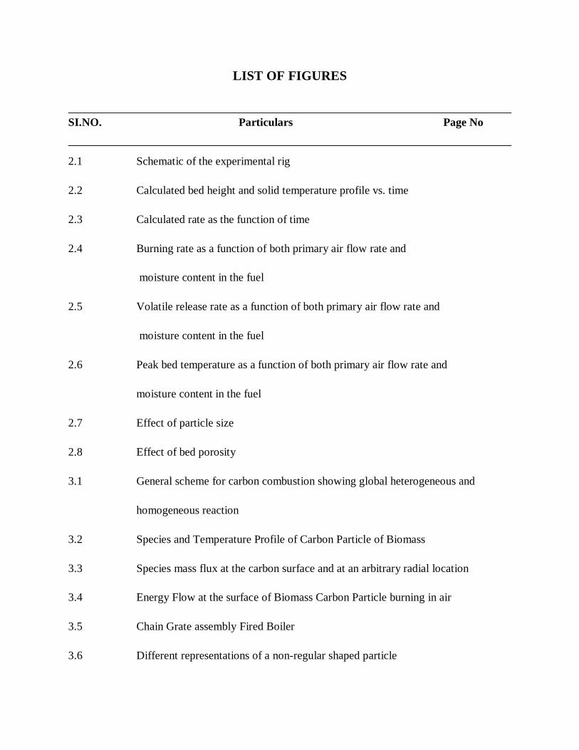
LIST OF FIGURES


2.1 Schematic of the experimental rig

2.2 Calculated bed height and solid temperature profile vs. time

2.3 Calculated rate as the function of time

2.4 Burning rate as a function of both primary air flow rate and

moisture content in the fuel

2.5 Volatile release rate as a function of both primary air flow rate and


2.6 Peak bed temperature as a function of both primary air flow rate and


2.7 Effect of particle size

2.8 Effect of bed porosity

3.1 General scheme for carbon combustion showing global heterogeneous and

homogeneous reaction

3.2 Species and Temperature Profile of Carbon Particle of Biomass

3.3 Species mass flux at the carbon surface and at an arbitrary radial location

3.4 Energy Flow at the surface of Biomass Carbon Particle burning in air

3.5 Chain Grate assembly Fired Boiler

3.6 Different representations of a non-regular shaped particle

4.1 Furnace different level

4.2 Two stage superheater - Primary and Secondary

4.3 Boiler Bank - Cross Flow (Typical)

4.4 Boiler Bank Screen (Typical)

4.5 Economizer

4.6 Behavior of particle burning time with respect to biomass size

4.7 Variation of burning rate as the function of biomass aspect and pressure

4.8 Least variation of heat release from bed with corresponding bed temperature

4.9 Fuel bed density Vs. Fuel bed heat release to near furnace wall

4.10 Variation of Non-luminous radiant coefficient with gas temperature

4.11 Primary super heater tube OD vs. Convective Coefficient

4.12 Behavior of convective coefficient with boiler fuel loading

4.13 Super Heater internal diameter Vs. Internal heat transfer coefficient

4.14 Behavior of Internal heat transfer coefficient with boiler fuel loading

4.15 Boiler fuel loading vs. Heat transfer to cavity wall

4.16 Pressure drop in fuel bed with initial staged void value of wood particle

4.17 Pressure drop in fuel bed with varying void value with respect to primary air

velocity

4.18 Bed void fraction Vs. Velocity of primary air

NOMENCLATURE

Symbol Abbreviation

PA Primary Air

dv Volume Diameter

ds Surface Diameter

dp Sieve Size

dsv Surface-Volume Diameter

Ø Sphericity

qv Heat Release Rate per unit volume

qF Heat Release Rate per Unit Cross Sectional Area

qb Heat Release Rate per Unit Wall Area of the Burner Region

Yo2,s Concentration of oxygen in particle surface

Yo2, ∞ Concentration of oxygen in away from surface

Ts Temperature at surface

T∞ Temperature away from surface,K

휗 Mass stoichiometric coefficient

Kc Kinetic rate constant coefficient (m/s)

ρD Productofdensityandmassdiffusitivity

Tsur Surroundings Temperature, K

Cpg Specific Heat of gas (J/Kg-K)

KB Burning Rate Constant, m2/s

푡 Burning time of biomass particle, s

Do Diameter of Biomass Particle, m

LHV Lower Heating Value of fuel, KJ/Kg

V Furnace Volume, m3

B Designed fuel consumption rate, Kg/s

F Cross sectional area of the furnace grate m2

Nu Nusselt Number

Re Reynolds Number

Pr Prandtl Number

휌 Average density of fuel bed in furnace

푇 Average temperature of fuel bed

퐾 Thermal conductivity of the flue gas in W/mo C

휇 Dynamic viscosity of flue gas in kg/ms

ℎ Non-Luminous Radiative Coefficient, KJ/m2h °C

푡 Gas temperature in ° C

MBL Mean beam length in m

Tw Log mean wall temperature in o K

KE Wall emissivity correction factor

D Outside diameter of tube in m

푡 Film temperature in o C

R Fire bed (grate) surface area, m2

H Surface area of heat transfer (water wall), m2

휀 Emissivity of bed

휀 Emissivity of wall

휀 Emissivity of furnace gas

푎 Absorptivity of furnace gas

휌 Pressure of species A

푁 Total number of moles of species A in the volume V

푝 Total pressure exerted by the gas mixture

∆ Pressure drop across fuel bed , N/m2 per m of fuel depth

휀 Void fraction in the bed

U Gas flow rate per unit cross section of the bed, m/s

Abstract

ABSTRACT

BIOMASS ASPECT AND AIR VELOCITY MODELING FOR COMBUSTION CUM

HEAT TRANSFER ENHANCEMENT IN GRATE FIRED BOILER

By

J.Elamathi Raja

Degree : Master of Technology

Guide : Mr.Sanjay Dasrath Dalvi



College of Engineering Studies

University of Petroleum and Energy Studies

Dehradun – 248 006

May, 2011

The biomass combustion in the furnace is depend on physical (Moisture content and

particle size) and chemical property (fuel composition) of fuel as well as furnace design and its

environment like mass flow rate of oxygen, particle residential time, temperature, turbulence and

velocity of combustion air. The mostly physical and chemical property of fuel cannot be greatly

controlled but the biomass particle size and the combustion velocity can be handled manually to

have the change in combustion behavior.

Also the heat transfer inside the furnace is the function of fuel combustion rate and

furnace components design parameters. The combustion rate of wide biomass aspect was

calculated whose result shows the burning rate increases with increase in pressure of impinging

primary air. The fuel bed heat release rate have minimal changes from 87.94 W/m2 K to 86.30

W/m2 K over wide range of the fuel bed temperature from 1900 K to 1200 K.

But when the fuel bed density vary from 800 to 500 Kg / m3, the heat release have wide

variation of about 92.8 W/m2 K to 77.27 W/m2 K. The Non-luminous radiative coefficient at

adiabatic flame temperature of wood (1627 o C) is 389.46 KJ/m2 h °C, but in actual it is about

257.92 KJ/m2 h °C at 1100 o C of fuel bed temperature.

The convective coefficient tends to increase about 15 -20 % (From 0.86 to 1 W/m2 o C)

with about 30 % reductions in OD of superheater (From 50.8 mm to 35 mm) and the maximum

heat absorption take place by heat radiation. The wood piece of 6 cm long and 3 cm diameter

have customized pressure drop between 3mm to 5 mm of WC per mm of fuel bed depth between

11 m/s to 15 m/s of air velocity which will result in enhanced combustion.

Key words: Biomass combustion; particle size; air velocity; fuel bed heat rate; Non-luminous

radiative coefficient; Convective coefficient; fuel bed pressure drop.

Introduction

CHAPTER I

INTRODUCTION

1.1 Biomass Combustion

Biomass combustion represents a possibility to lower regional emissions of the greenhouse

gas CO2, especially in countries with large wood resources. In India, potential of energy generation

through biomass is about 22000 MW out of which we achieved only 2437 MW (MNRE, 2010).

Despite the ecological advantages of renewable energies, a techno-economic optimization of the

combustion unit is necessary in order to make biomass-fired heating plant competitive with

fossil fuel-fired systems. The major goal of the development and optimization of biomass grate

furnaces is the reduction of investment and operating costs. This can be achieved by a compact

furnace design, an increased availability of the plant, by reduced emissions (CO and NOx) as well

as by reduced air and flue gas fluxes in the furnace. The design of biomass furnaces is still usually

based on experience and empirical data.

1.2 Grate boiler in glance

Boiler is the mean to have combustion of fuel & transferring the resulting energy of

combustion to working fluid called water which is converted in to steam after absorbing the

energy which again used for driving a mechanical device or process heat application. Grate fired

boiler are widely used in industrial application for its ability to handle high moisture content fuel

and wide range of fuel input. While operation of this boiler about 15 – 20% of energy is loosed

through heat along flue gas (7 to 10%), evaporation of water formed as a result of hydrogen

oxidation (7%) and surface radiation & unaccountable loss (2%) (BEE, 2005).

This study is about bringing down the energy loss in flue gas to maximum extent by

increased heat transfer of hot gas to working fluid & achieving complete combustion with least

excess air by experimenting the biomass combustion phenomena with different biomass aspect

(size) and combustion air velocity there by its effect on carbon burnout, excess air requirement,

residential time for particle combustion, heat release rate, composition of gas, distribution path of

hot gas within the furnace geometry and temperature distribution of hot gas is examined and

optimized biomass size & air velocity is chosen with respect to achieve less excess air

requirement, maximum heat release rate, maximum heat transfer between hot gas & water wall

tubes within furnace geometry. The effectiveness of biomass combustion mainly depends on its

particle size (exposed surface area) & mass flux of oxygen which have relation with its velocity.

So these two main factors are going to be analyzed in this study (Sridharan, 2008).

Grate fired boiler have to handle wide range of fuel with different bandwidth of moisture

content, so it’s necessary to establish the optimum size of biomass and combustion air velocity to

achieve maximum combustion efficiency. These grate boilers are characteristics with slow

response to load swing because of high fuel loading on grate. To overcome this problem detail

study upon various fuel factors (like Moisture content, particle size, mass flow rate of oxygen,

composition, residential time, velocity of combustion air) and its influence on combustion need

to be done. But invariably control of particle size and combustion air parameters are only left to

us to make regulation upon combustion. So these parameters are selected for the analysis.

1.3 Biomass power plant

The most efficient method of using bio-mass would be for power generation purposes.

The bio-mass boilers would produce steam which will be fed to steam turbine producing

electrical power. The steam turbines work on the Rankine Thermo Dynamic Cycle. Rankine

Cycle gives better efficiencies with the increase in pressure and temperature of the steam fed to

the turbine. The turbine designs have their own special features which make certain steam

temperature regimes attractive with certain specific steam pressure regimes. These ranges of

steam pressure and their corresponding ranges of steam temperature are given in Table 1.1.

Table 1.1 Preferred pressure temperature combinations at inlet to steam turbines

S.No Steam inlet pressure (ATA) Preferred steam inlet temperature (Deg C)

1 32 435

2 41 455

3 62 485

4 86 510 / 538

5 103 and above 538 / 635

It should always be desirable to go in for as high a steam pressure and temperature as

possible. However, going in for higher steam temperature for certain specific pressure values

have limitations with regard to boilers firing bio-mass fuels (Sridharan, 2008).

With higher steam temperatures and pressures, it becomes necessary that greater

percentage of total heat of steam generation be given in the super heater. It then becomes

necessary that the flue gasses leaving the furnace must have higher and higher temperatures, in

order to cater to this higher percentage of super heat requirements (Sridharan, 2008).

Table 1.2 Recommended Flue Gas Temperatures at Furnace Outlet for Achieving Various

Superheat Steam Temperatures

S.No Super heat steam temperature (o C) Required furnace exit gas temperature (o C)

1 Up to 380 o C Above 600 o C

2 380 – 420 o C Above 650 o C

3 420 – 480 o C Above 700 o C

4 480 – 520 o C Above 750 o C

5 520 – 540 o C Above 980 o C

It becomes evident from the Table 1.2 that the ash fusion characteristics of the bio-mass

fuel will have a definite influence on the allowable flue gas temperature on furnace outlet. The

flue gas temperatures at furnace outlets should be 100°C less than the ash fusion temperature.

This feature imposes restriction on the super heat temperature that can be achieved in a boiler

with a given bio-mass fuel. Most of the bio-mass fuels are therefore not amenable for super heat

temperature of 515°C and above. They are also non-amenable for adoption with re-heat cycles

The higher moisture content in the biomass fuels lead to higher moisture content in the

flue gas evolved. The non-luminous radiation characteristics of flue gas are greatly influenced by

the quantity of water content in them. Flue gasses with high water content give raise to higher

non-luminous radiation. The bio-mass fuel fired boilers should take this into consideration while

assessing the total heat transfer across various heating surfaces in such boilers.

The higher moisture content of flue gasses also lead to higher dew point of these flue

gasses. The low temperature heating surfaces in biomass fired boilers are therefore susceptible to

low temperature corrosion due to moisture. The design of air pre-heaters for biomass fired

boilers should take this aspect into account (Sridharan, 2008).

The biomass is a promising fuel alternative for power generation. Since, the biomass is

created by "Carbon fixation" the combustion of biomass is not disturbing the delicate "carbon di-

oxide balance" of the atmosphere. The adoption of bio-mass as a fuel for power generation

should therefore be encouraged.

1.4 Objectives

1. To optimize operational loading of boiler for enhancing boiler Combustion & heat transfer

2. Experimenting combustion with different biomass aspect cum combustion air velocity for

optimizing biomass size and primary air supply pressure

3. To study the radiative heat transfer and convective heat transfer from fuel bed and flue gas to

furnace water wall surface

4. To study the design of selected boiler components and its influence on heat transfer coefficient

Review of Literature

CHAPTER II

REVIEW OF LITERATURE

This chapter consists of previous work carried out in the field of biomass combustion

modeling with respect to primary air velocity, biomass size distribution and heat release rate and

their studies are categorized under the following subtopics.

2.1 Combustion of biomass in packed bed

2.2 Mathematical description of biomass and solid waste combustion on a packed bed

2.3 Experimental facilities

2.4 Bed height, solid temperature and reaction zone thickness vs. time

2.5 Process rates vs. time and combustion stages

2.6 Time-averaged burning rate vs. primary air flow rate and moisture level

2.7 Devolatilisation rate vs. primary air flow rate and moisture level

2.8 Char burning rate vs. primary air flow rate and moisture level



2.1 Combustion of biomass in packed bed

Combustion of biomass and municipal solid wastes can be accomplished in packed beds,

either static or moving. The design, operation and maintenance of such combustion equipment

require detailed understanding of the burning process inside the bed. There have been many

researches into packed bed combustion of solid fuels, mainly biomass and wastes during the last

two decades. The propagation of a reaction front in a packed bed for thermal conversion of

municipal waste and biomass was investigated by Gort (1995). The distribution of temperature

and gas composition in a bench-top packed bed burning simulated waste (SW) fuels has been

measured by Goh et al., (1999). Other researchers include Zakaria et al., (2000) who investigated

the reduction of NOx emission from the burning bed in a municipal solid waste incinerator and

Ro¨nnba¨ck et al., (2000) who studied experimentally the influence of primary airflow and

particle properties on the ignition front, its temperature and on the composition of the exiting

gases in a biomass fuel bed.

Measurements on medium or large-scale moving beds were also carried out by Sharifi

(1990) in which detailed measurements of waste properties, bed temperature and gas

composition profiles were reported. Measurements on gasification of waste materials in a

medium-scale grate system were done by Beckmann et al., (1997). The latest full scale

experiments on moving grates were reported by Thunman et al., (2001) and Yang et al., (2002).

However, there is still a lack of detailed and systematic theoretical study on the packed

bed burning of biomass and municipal solid wastes. The advantage of theoretical study lies in its

ability to reveal the detailed structure of the burning process inside a solid bed, such as reaction

zone thickness, combustion staging, gas emission and char burning characteristics, thus

contributing to better understanding and controlling of the process. These parameters are hard to

measure by conventional experimental techniques.

The authors have previously investigated the effects of fuel devolatilisation and moisture

level on the combustion of wood chips and incineration of simulated municipal solid wastes in a

packed bed by Yang et al., (2002) and it was found that the kinetic devolatilisation rate has

noticeable effects on the ignition time, peak flame temperature, CO and H2 emissions at the bed

top and the proportion of char burned in the final stage (char burning only) of the combustion;

and also a wetter fuel results in a thinner reaction zone in the bed. In this paper, the work is

extended to the effect of primary airflow rate for biomass and municipal solid wastes.

Primary airflow is employed as a major controlling parameter to maintain the stability of

the combustion and achieve the desired burning rate, temperature and gas composition. In this

paper, the same mathematical model as in previous work by Yang et al., (2002) is employed and

extensive calculations carried out to assess the combined influence of the primary airflow and

moisture level on the burning behavior of biomass and simulated municipal solid wastes in a

static bed. Limited experimental work was also done to validate the calculations. The current

research contributes to better understanding of the biomass and waste combustion processes

2.2 Mathematical description of biomass and solid waste combustion on a packed bed

Peters (2003) summarized the previous mathematical models on packed bed combustion.

Those models can be generally classified into four categories: continuous-medium models where

the solid bed was treated as a continuous medium; neighboring-layers models where the packed

bed above the grate was divided into four layers representing fuel, drying, pyrolysis and ash;

well stirred reactor models where the bed was simulated by a cascade of well-stirred reactors;

and the 1d + 1d model where a one-dimensional and transient single-particle model in spherical

coordinates was implemented in a transient one-dimensional fuel-bed model.

A packed bed, either stationary or moving, consists of numerous individual particles and

the gaps between them through which combustion air flows. Ideally, calculations should be made

both outside and inside the solid particles. But the shear number of the individual particles in the

bed prevents such delicate calculations to be performed on the whole bed due to an unrealistic

requirement for CPU speed and computer memory. In fact, the temperature profile inside a

particle is three-dimensional (not one-dimensional in respect of the radial distance) and this

further adds to the difficulty. In the light of this, in this study the whole bed is treated as a

continuous porous medium and numerical calculations are carried out by dividing the bed into

many cells. Inside each cell the concerned parameters (e.g. temperature, percentage of moisture,

carbon, etc.) are assumed uniform and by reducing the cell size (hence increasing the cell

number), calculation can be made on a size-scale much smaller than the fuel particles. For the

fuels used in this work (size around 12 mm), the Biot number is calculated as being around 1.0.

So no significant errors are expected to occur due to the non-isothermal behavior of the solids.

The solid fuel is assumed to consist of four components, moisture, volatile matter, fixed carbon

and ash (Yang et al., 2003).

The incineration process of solid wastes can be divided into four successive sub-

processes: evaporation of moisture from the solids, volatile release/char formation, burning of

the hydrocarbon volatiles in the gaseous space, and the combustion of char particles. The

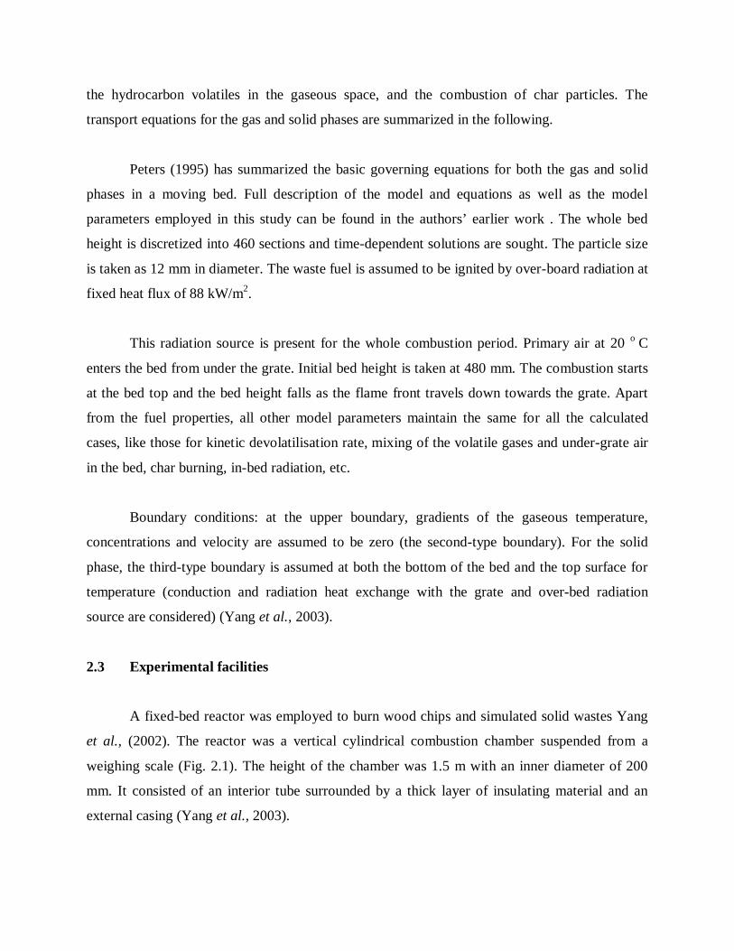
transport equations for the gas and solid phases are summarized in the following.

Peters (1995) has summarized the basic governing equations for both the gas and solid

phases in a moving bed. Full description of the model and equations as well as the model

parameters employed in this study can be found in the authors’ earlier work . The whole bed

height is discretized into 460 sections and time-dependent solutions are sought. The particle size

is taken as 12 mm in diameter. The waste fuel is assumed to be ignited by over-board radiation at

fixed heat flux of 88 kW/m2.

This radiation source is present for the whole combustion period. Primary air at 20 o C

enters the bed from under the grate. Initial bed height is taken at 480 mm. The combustion starts

at the bed top and the bed height falls as the flame front travels down towards the grate. Apart

from the fuel properties, all other model parameters maintain the same for all the calculated

cases, like those for kinetic devolatilisation rate, mixing of the volatile gases and under-grate air

in the bed, char burning, in-bed radiation, etc.

Boundary conditions: at the upper boundary, gradients of the gaseous temperature,

concentrations and velocity are assumed to be zero (the second-type boundary). For the solid

phase, the third-type boundary is assumed at both the bottom of the bed and the top surface for

temperature (conduction and radiation heat exchange with the grate and over-bed radiation

source are considered) (Yang et al., 2003).

2.3 Experimental facilities

A fixed-bed reactor was employed to burn wood chips and simulated solid wastes Yang

et al., (2002). The reactor was a vertical cylindrical combustion chamber suspended from a

weighing scale (Fig. 2.1). The height of the chamber was 1.5 m with an inner diameter of 200

mm. It consisted of an interior tube surrounded by a thick layer of insulating material and an

external casing (Yang et al., 2003).

Fig 2.1 Schematic of the experimental rig

The grate was located at the bottom of the chamber and consisted of a perforated plate

made from stainless steel, with approximately 700 holes of 2 mm diameter, representing 7%

open area.

Thermocouples were used to monitor the temperature of primary airflow, temperature

inside the bed at different height levels and temperature of the flue gases. There was a gas-

sampling probe inside the chamber at 430 mm above the grate. A gas burner was placed at a 458

angle toward the waste at 750 mm above the grate. The gas burner was used to initiate the

burning process of the waste sample and for maintaining the free-board combustor temperature

during the experiment. Primary air was fed from the bottom of the fixed-bed reactor through the

grate without preheating (Yang et al., 2003).

2.4 Bed height, solid temperature and reaction zone thickness vs. time

Fig. 2.2 shows the calculated bed height and solid temperature profile vs. time for the

combustion of SW containing 31% moisture in the bench-top incinerator. The initial bed height

is 480 mm above the grate and the primary air flow rate is 0.13 kg/m2 s. The inlet air temperature

is 15 o C. It is seen that the bed top begins to fall at t = 200 s as the local bed temperature rises

from room level to above 900 K.

Later the temperature at the bed top increases to 1300 K while the height of the bed

decreases linearly. From around t = 400 s, the bed-top temperature begins to fall to around 1100

K and remains at that level for a considerable time period. During this time, the height of the bed

continues to drop linearly. It is also seen that the flame front reaches the bottom of the bed (the

grate) at around t = 1100 s.

After that, the bed becomes very hot for a short period of time and the maximum

temperature goes up to 1500 K. This lasts about 200 s during which time the height of the bed

undergoes only a slight fall. Further on, the bed residual material cools down as the combustion

completes at t = 1450 s. It is also interesting to note the development of the reaction zone as time

goes on (Yang et al., 2003).

The thickness of the reaction zone is defined as the distance from the bed top downward

to where the bed temperature begins to rise from the original room temperature. Fig. 2.1 shows

that as the bed gets ignited from the top at around t = 100 – 200 s, the reaction zone thickness

increases quickly to about 14 mm or roughly one particle diameter.

Fig 2.2 Calculated bed height and solid temperature profile vs. time (SW, 30% moisture, initial

bed height = 480 mm, primary air = 0.13 kg/m2 s at 15 8C).

With the combustion proceeding, the reaction zone thickness increases and reaches a

maximum level of 96 mm or 8 times of the original particle diameter when the flame front

touches the bed bottom. After that, the reaction zone extends to the whole bed height for a while

before receding towards the bed top as the char burns out (Yang et al., 2003).

2.5 Process rates vs. time and combustion stages

Fig. 2.3 shows the corresponding calculated individual process rates as a function of time

for the case shown in Fig. 2.2. The individual process rates are for moisture evaporation,

devolatilisation and char combustion. Three stages are identified. The first is the initial or

ignition stage (t = 0 – 100 s) where only moisture evaporation occurs (Yang et al., 2003).

The moisture inside the solids is driven out at temperature of 100 o C by strong radiation

from the over-bed ignition source. When all the moisture in the top layer has been evaporated,

the local bed temperature then rises quickly to the onset point of devolatilisation (taken as 260 o

C or 533 K) at t = 100 s and the bed is ignited. There is a temporary fall in the moisture

evaporation rate just before the bed ignition. This is because the over-bed heat input to the

evaporation front inside the bed decreases as the front moves away from the bed top downward.

After that, the moisture evaporation rate recovers as the heat supply shifts from over-bed to the

newly established flame-front at the bed top (Yang et al., 2003).

Fig 2.3 Calculated rate as the function of time

(SW,30% moisture, initial bed height = 480 mm, primary air = 0.13 kg/m2 s at 15 0 C).

The primary burning stage starts after the bed gets ignited at t = 100 s and extends to

where both the moisture and the volatiles in the whole bed have been completely driven out at t =

1200 s. It takes over 70% of the total combustion time. During this period, moisture evaporation,

devolatilisation and char burning rates maintain a relatively constant level, respectively (the

formed char begins to burn at t = 200 s as the local solid temperature reaches a preset onset

temperature of 600 o C or 873 K). Towards the end of this primary stage, the devolatilisation rate

shows a sharp rise before falling to zero (Yang et al., 2003).

This is because all the moisture has evaporated at this point, causing an upsurge in the

bed temperature. The final stage of combustion follows where only char burning occurs. An

initial sharp increase in the char burning rate is shown and this is due to the increased O2

availability to the char burning (in the primary stage, most of the O2 is consumed by volatile gas

burning). The char burning rate falls gradually as time goes on until the whole combustion

process completes at t = 1500 s. The final stage comprises 20% of the total combustion time. Fig.

2.3 also shows the calculated total mass loss rate as a function of time compared to experimental

measurement. Agreement between the two is reasonably good. The total mass loss rate is a

summation of moisture evaporation, volatile release and char burning (Yang et al., 2003).

2.6 Time-averaged burning rate vs. primary air flow rate and moisture level

Fig. 2.4 shows the time-averaged burning rate on a dry basis as a function of primary air

flow rate at different moisture levels for SW, wood cubes and forest wastes. The particle size

ranged from 10 to 20 mm though for theoretical calculations it was fixed at 12 mm.

Experimental data, especially from Gort (1995) have clearly established the patterns for the

relationship between the burning rate and the air flow rate at different moisture levels.

However, a systematic theoretical calculation employing proper mathematical models

has not been done previously and the results shown here are intended to demonstrate the

reasonably good agreement between the modeling predictions and experimental measurements.

This gives validity for the following detailed. Theoretical analysis of the combustion processes.

The airflow rate spans a range from 0.03 to 0.6 kg/m2s without preheat (around 15 o C) and the

moisture level covers from 10 to 50% on a wet basis.

At a certain moisture level, the burning rate increases as the airflow rate increases until a

peak point is reached, beyond which a further increase in the air flow results in a fall in the

burning rate. This is defined as the critical air flow rate and reflects the balance between the

burning heat absorbed by the solids and the heat loss to the cooler gas stream from the particles.

Thus at lower air flow rates, more heat is generated than that carried away by the gas flow.

At higher flow rates, however, the heat carried away by the gas flow exceeds the heat

generated by combustion. The effect of moisture level in the fuel is obvious. At a fixed airflow

rate, drier fuels have higher burning rates while wetter fuels have lower burning rates. For

example, at 10% moisture the maximum burning rate obtainable (the peak point at the critical air

flow rate) by experiments was 0.07 kg/m2 s while at 50% moisture it was only 0.018 kg/m2 s,

nearly 4 times lower.

Fig 2.4 Burning rate as a function of both primary air flow rate and moisture content in the fuel.

The critical air flow rate corresponding to each of the peak burning rates is also affected

by the level of moisture. Calculations show that a drier fuel has a higher rate and a wetter fuel

has a lower one. Results of the theoretical calculation and the experiments can be compared.

Agreement is satisfactory to good in terms of the general trends. However, the calculated burning

rate is higher than the measured one at high primary air flow rates. This might be caused by the

channeling phenomenon at a high airflow rate in an actual bed. The local bed structure (porosity,

particle size distribution and the orientation of particles) cannot be made perfectly uniform in an

actual bed. The effect of such structure non-uniformity on the flow distribution inside the bed

can become significant at high flow rates and channeling occurs as a consequence, where some

of the combustion air would bypass the solids and flows out of the bed without reacting, thus

reducing the burning efficiency. The current mathematical models did not take the channeling

into account (Yang et al., 2003).

2.7 Devolatilisation rate vs. primary air flow rate and moisture level

Fig. 2.5 shows the calculated time-averaged devolatilisation rate as a function of both air

flow rate and moisture level. Similar trends to the situations of the burning rate are found for the

devolatilisation rate in relation to the change in the air flow rate. The moisture level also

demonstrates a strong effect and the drier the fuel, the higher its devolatilisation rate. For

example, the maximum devolatilisation rate for 10% of moisture is obtained as 0.08 kg/m2 s,

compared to only 0.028 for 40% of moisture.

The volatile release rate is a strong function of temperature. Drier fuels require less heat

for moisture evaporation and the reaction zone is thicker Yang et al., (2002). The moisture

evaporation front is moved away from the devolatilisation front so that less heat is transferred

from the devolatilisation zone downward to the moisture evaporation zone, resulting in a higher

temperature in the devolatilisation zone which enhances the devolatilisation rate.

2.8 Char burning rate vs. primary air flow rate and moisture level

There are two stages involving char burning, the primary stage and the final stage. In the

primary stage, the char burning rate is affected by both the primary air flow rate and the moisture

level in the fuel. It is seen that at any fixed moisture level greater than 10%, the char burning rate

in the primary stage rises as the primary air flow increases and reaches a peak point at the critical

air flow rate. After that the rate declines as the air flow is further increased.

This is in line with the total burning rate shown in Fig. 2.4. For the moisture level at

10%, however, the char burning rate undergoes a continuous rise as the primary air increases in

the whole covered range. The moisture level also affects the char burning rate in the primary

stage. Firstly, the critical air flow rate at which the char burning rate reaches a maximum shifts to

a greater value for a drier fuel. For example, the critical air rate is 0.2 kg/m2 s for 40% moisture,

but increases to 0.32 kg/m2 s for 20% moisture. Secondly, in the range where the air flow is

lower than the critical rate (at a given moisture level), a wetter fuel, surprisingly, has a higher

char burning rate than a drier fuel at the same air flow rate. This is not clear for the cases of 10

and 20% moisture, however (Yang et al., 2003).

.

Fig 2.5 Volatile release rate as a function of both primary air flow rate and moisture content

in the fuel. The moisture level ranges from 10 to 50% on a wet basis. The fuels are 12-

mm simulated wastes (SW). The over-bed radiation heat flux is fixed at 88 kW/m2.

It is also interesting to look at the percentages of char burned in the primary

and final stages. The amount of char burned in the final stage takes the balance. It is seen

that the percentage of char burned in the primary stage increases roughly linearly with increase

in the primary air flow (Yang et al., 2003).

At each moisture level, there is a critical air flow rate at and beyond which all the char is

burned in the primary stage and the final or the char-burning-only stage no longer exists. The

moisture effect is significant. The wetter the fuel, the higher the percentage of char burned in the

primary stage. For the wettest fuel, all the char is burned in the primary stage even at small air

flow rates. The char burning depends on three factors: the amount of formed char, the O2

availability and the temperature. The relationship between its rate and the primary air flow can

be explained in terms of those three factors. In the range of air flow smaller than the critical rate

(at a given moisture level), an increase in the air flow makes more O2 available to the char

burning. It also increases the devolatilisation rate as demonstrated in Fig. 2.5 (so more char is

produced) as well as the flame temperature (as shown later in Fig. 2.6).

When the air flow rate is further increased beyond the critical point, the flame

temperature undergoes no further increase (Fig. 2.6) and the devolatilisation rate starts to

decrease (Fig. 2.5) so less char is produced, though more air is available to the char burning. The

moisture effect can be explained in the following way (Yang et al., 2003).

Fig 2.6 Peak bed temperature as a function of both primary air flow rate and moisture content in

the fuel. The moisture level ranges from 10 to 50% on a wet basis. The fuels are 12 mm

simulated wastes (SW) unless indicated otherwise. The over-bed radiation heat flux is fixed at 88

kW/m2 for the calculations (Yang et al., 2003).

A wetter fuel reduces the devolatilisation rate and hence the O2 consumption by the

burning of the volatile gases. This makes more O2 from the air supply available to the char

burning in such a way that overweighs the effect caused by decreasing char formation, so the net

effect is an increase in the char burning rate compared to a drier fuel (Yang et al., 2003).


The particle size covered in the calculations ranges from 2 to 35 mm. Fig. 2.7(a) shows

the burning rate as a function of particle size at different primary air velocities. Generally, larger

particle size results in lower burning rate. For instance, 5 mm particles have a burning rate of

0.06 kg mK2 sK1 at a primary air velocity of PA3, which is 1.5 times of the burning rate with 30

mm particles at the same primary air velocity. One exception is for the particle sizes of 4 and 5

mm at the primary air velocity PA2 where the 5 mm particles demonstrate a higher burning rate

than the 4 mm particles. Fig. 2.7(b) shows the combustion stoichiometry as a function of particle

size. Generally, larger-size particles result in a higher air-to-fuel stoichiometric ratio or less

fuelrich combustion. For instance, 5 mm particles have an airto- fuel stoichiometric ratio of 0.49

at PA3 compared to the ratio being 0.74 with 30 mm particles at the same conditions.

One exception is for particle sizes of 4 and 5 mm at the primary air velocities PA2 and

PA3 where the 5 mm particles produce a slightly fuel-richer condition than the 4 mm particles.

Fig. 2.7(c) shows the bed-top gas composition as a function of particle size.For CO, the

volumetric percentage ranges from around 12 to 17% and larger particles have lower CO levels

at the bed top; for CH4, the volumetric percentage ranges from 5 to 9% and a noticeable change

in the relationship with the particle size is only obtained for particles smaller than 5 mm at PA1,

for particles smaller than 10 mm at PA2 and for particles smaller than 15 mm at PA3. Generally,

increasing particle size reduces the methane concentration at the bed top. For H2, the volumetric

percentage ranges from 1.5 to 7% and generally an increase in particle size results in higher

hydrogen concentration at the bed top (Yang et al., 2003).

Fig 2.7 Effect of particle size: (a) average burning rate; (b) combustion stoichiometry; (c) gas

composition at the bed top; (d) maximum solid temperature.

The primary air velocity has negligible effect on H2 when particles are smaller than 10

mm. It also has negligible effect on CO when particle size is greater than 20 mm. Fig. 2.7(d)

shows the maximum solid temperature inside the bed as a function of particle size. It is seen that

at PA1 the maximum solid temperature increases as particle size increases from 2 to 3 mm, then

drops down 30 K at 4 mm, rises again at 5 mm to the maximum level of 1270 K. Beyond 5 mm,

the general trend is decreasing solid temperature as particle size increases. At 35 mm, the

maximum solid temperature is 70 K lower than the peak value obtained at 5 mm.

At PA2, the maximum solid temperature pattern in relation to the particle size is similar

to the case of PA1, except that the absolute temperature level is about 50 K higher on the whole.

At PA3, the maximum solid temperature is obtained at 4 mm (1350 K) but falls to 1320 K at 5

mm. Over the range of 10–20 mm, the maximum solid temperature maintains a constant level of

1335 K.


Bed porosity depends on a number of factors, including particle size distribution, particle

shape, shaking or pressing of the bed, etc. A bed with a low porosity is called a compact bed and

a bed with a high porosity is called a loose bed. In this section, the initial bed porosity is

artificially changed while keeping all the other bed parameters the same. The porosity covers a

range of 0.35–0.75. Fig. 2.8(a) demonstrates the effect of bed porosity on the burning rate of the

bed. It is seen that the effect of bed porosity depends on the level of primary air velocity. At low

primary air velocities (PA1 and PA2), the general trend is decreasing burning rate as the bed

porosity increases, though in some ranges the burning rate may maintain a more or less constant

level (porosity 0.5–0.65 for PA1 and 0.65 onwards for PA2) (Yang Bin et al., 2005).

Fig 2.8 Effect of bed porosity: (a) average burning rate; (b) combustion stoichiometry; (c) gas

composition at the bed top; (d) maximum solid temperature

At increased primary air velocity (PA3), the maximum burning rate is obtained between

bed porosity of 0.45–0.55 and either a looser or denser bed would results in a lower burning rate.

However, similar to the situation of PA2, the burning rate keeps constant as the bed porosity

increases beyond 0.65. Fig. 2.8(b) demonstrates the combustion stoichiometry against the initial

bed porosity. Generally, the air-to-fuel stoichiometric ratio increases as the bed porosity

increases (Yang Bin et al., 2005).

But the air-to-fuel ratio keeps constant in some part along the range, i.e. bed porosity

from 0.5 to 0.65 for PA1 and from 0.65 onwards for PA2 and PA3. Fig. 2.8(c) shows the bed-top

gas composition as a function of bed porosity. For CO at PA1, very little change in its level is

shown for the whole range of porosity variation; for CO at PA2, the volumetric level in the flue

gases exiting the bed top falls in the range of 0.45–0.6 of the bed porosity, otherwise, it keeps a

constant value; for CO at PA3 the maximum level is obtained around a bed porosity of 0.45 and

either a looser or denser bed results in a lower CO concentration at the bed top. For CH4 at PA1

and PA2, the general trend is reducing concentration level as the bed porosity increases; for CH4

at PA3, the maximum level is obtained around the bed porosity of 0.5. It is also seen that the H2

concentration is not affected by either the bed porosity or the primary air velocity. Fig. 2.8(d)

demonstrates the maximum solid temperature against porosity variation (Yang Bin et al., 2005).

The pattern of variation depends on the primary air velocity. At the low air velocity of

PA1, the maximum solid temperature rises as the bed porosity rises from 0.35 to 0.45, but keeps

constant from 0.45 to 0.55, falls from 0.55 to 0.65 and then rises again from 0.65 onwards. At

PA2, however, a continuous increase in the solid temperature is obtained as the bed porosity

increases from the minimum to the maximum. For the situation of PA3, the solid temperature

increases with increasing bed porosity until the porosity reaches 0.65, followed then by a fall in

the maximum solid temperature as the bed porosity further increases (Yang Bin et al., 2005).

.

Model Development

CHAPTER III

MODEL DEVELOPMENT

In this chapter models and methodology used for determining the burning rate of biomass

and heat transfer in furnace is discussed under the following sub headings.

3.1 Biomass Combustion rate and burning time model

3.1.1 One film model

3.1.1.a Assumptions

3.1.1.b Overall mass and species conservation

3.1.1.c Energy Conservation Equation application for Biomass Particle

3.1.2 Particle Burning Time

3.2 Modeling of biomass combustion on grate

3.3 Characteristics of solid particle

3.3.1 Solid particles

3.3.2 Equivalent diameters

3.3.3 Volume Diameter (dv)

3.3.4 Surface Diameter (ds)

3.3.5 Sieve Size (dp)

3.3.6 Surface-Volume Diameter (dsv)

3.3.7 Sphericity (Ø)

3.3.8 Packing characteristics

3.4 Biomass Characterizations

3.5 Fundamental of Grate Fired Boiler Design and Operation

3.5.1 Combustion air system and temperature

3.5.2 Moving Grate Boiler Grate Design

3.5.3 Fuel Bed Thickness

3.5.4 Furnace Design

3.5.5 Firing Rate of Furnace

3.5.5. a Heat Release Rate per unit volume (qv)

3.5.5.b Heat Release Rate per Unit Cross Sectional Area (qF)

3.5.5.c Heat Release Rate per Unit Wall Area of the Burner Region (qb)

3.5.6 Furnace Depth

3.5.7 Furnace Height

3.5.8 Furnace Exit Gas Temperature

3.6 Heat and Mass Transfer in Furnace

3.6.1 Furnace Heat Transfer

3.6.2 Determining Heat Transfer Coefficient to the fuel particle in Fuel bed

3.6.3 Heat Transfer to the wall of the furnace near bed

3.6.4 Gas temperature at furnace exit

3.6.5 Determining flue gas property

3.6.6 Thermal Conductivity of flue gas

3.6.7 Determining Dynamic Viscosity of flue gas

3.6.8 Determining Non-luminous radiative coefficient

3.6.9 Determining Convective coefficient for cross flow

3.6.10 Radiative Heat Transfer

3.6.11 Mass Transfer

3.6.12 Diffusion mass transfer; molecular or eddy diffusion

3.6.13 Convective mass transfer: free or forced

3.6.14 Determining Velocity, concentration and flux of flue gas mixture

3.6.14.1 Concentrations

3.6.14.2 Velocities

3.6.14.3 Fluxes

3.7 Determining Pressure drop across bed of fuel in grate

3.1 Biomass Combustion rate and burning time model

Fig. 3.1 schematically shows the burning carbon surface within a reacting boundary

layer. At the surface carbon can be attacked by either O2, CO2 and H2O, depending primarily

upon the surface temperature, via the following global reaction

C + O2 = CO2 (3.1)

2C + O2 = 2 CO (3.2)

C + CO2 = 2CO (3.3)

C + H2O = CO + H2 (3.4)

Fig. 3.1 General scheme for carbon combustion showing global heterogeneous and homogeneous

reaction

The principle product at the carbon surface is CO. The CO diffuse away from the surface

through the boundary layer where it combine with the inward diffusion O2 according to the

following global homogeneous reaction

CO + ½ O2 = CO2 (3.5)

In principle, the problem of carbon oxidation could be solved by writing the appropriate

conservation equations for species, energy and mass, defining all of the elementary reaction steps

and then solving these equations subject to appropriate boundary condition at the surface and

free stream. The major complication to this scenario, however, is that the carbon surface is

porous and the detail nature of the surface changes as the carbon oxidation proceeds. Thus the

process of intraparticle diffusion plays the major role in combustion under certain condition.

Simplified model of carbon combustion rely on the global reactions and usually assumes

that the surface is impervious to diffusion. Depending upon the assumption made for both the

surface and gas phase chemistry, different scenario emerge which are generally classified as one

film, two film or continuous film models (Turns, 2000).

In the one film model there is no flame in the gas phase and the maximum temperature

occurs at the carbon surface. In the two film models, a flame sheet lies at some distance from the

surface, where the CO produced at the surface reacts with incoming O2 .In the continuous film

models, a flame zone is distributed within the boundary layer .rather than occurring in the sheet.

3.1.1 One film model

The one film model is quite simple to illustrate conveniently and clearly the combined

effects of heterogeneous kinetics and gas-phase diffusion. The two film model, although also still

quite simplified, is more realistic in that it shows the sequential production and oxidation of CO.

We then use these models to obtain estimates of carbon – char burning times (Turns, 2000).

The basic approach to the problem of carbon combustion is quite similar to treatment of

droplet evaporation expect the chemical reaction at the surface replaces evaporation. The burning

of single spherical carbon particle subject to the following assumption (Turns, 2000).

3.1.1.a Assumptions

1. Burning Process is Quasi – Steady

2. The biomass particle burns in a quiescent, infinite ambient medium that contain only oxygen

and inert gas such as nitrogen. There are other no interactions with others particle and the effect

of convections are ignored

3. At the particle surface the oxygen react with carbon particle to produce Carbon-di-oxide. In

general this reaction is not a particular good since carbon-di-oxide is preferred byproduct at

combustion temperature.

4. The gas phase consists of only O2, CO2 and inert gases. The O2 diffuses inward; react with

surface to form CO2, which then diffuse outward. The inert gas forms a stagnant layer as in the

Stefan Problem.

5.The gas phase Thermal Conductivity ,K, Specific Heat, Cp , and the product of density and

mass diffusivity ,ρD are all constant .Further more we assume that the Lewis Number is Unity,

i.e Le = k /( ρCpD) = 1.

6. The biomass particle is impervious to gas-phase species i.e. intra particle diffusion is ignored.

7. The particle is of uniform temperature and radiates as a gray body to the surroundings without

participation of the intervening medium (Turns, 2000).

Fig. 3.2 illustrate the basic model embodied by the above assumption ,showing how the

species mass fraction and temperature profile vary with the radial coordinates .Here we see that

the CO2 mass fraction is a maximum at the surface and is zero far from the particle surface. Later

we will see that if the chemical kinetics rate of O2 consumption is very fast, the oxygen

concentration at the surface, Yo2,s approaches zero. If the kinetics is zero, there will be an

appreciable concentration of O2 at the surface. Since we assume that there are no reaction

occurring in the gas phase and the entire heat rate occurs at the surface, the temperature

monotonically falls from a maximum at the surface, Ts to its value far from the surface, T∞.

Fig. 3.2 Species and Temperature Profile of Carbon Particle of Biomass assuming that CO2 is

only product of combustion at the Biomass Carbon Particle Surface.

Our primary objectives in the following analysis is to determine expression that allow

evaluation of the mass burning rate of the biomass carbon, mc and the surface temperature, Ts.

Intermediate variable of interest are the mass fraction of O2 and CO2 at the carbon surface. The

problem is straight forward and required dealing with only species and energy conservation.

3.1.1.b Overall mass and species conservation

The relationship among the three species mass fluxes,푚" , 푚" and 푚" is illustrated in

the Fig. 3.3. At the surface the mass flow of carbon must equal the difference between the

outgoing flow of CO2 and incoming flow of O2, i.e

푚" = 푚" −푚" (3.6)

Similarly at any arbitrary radial position, r, the next mass flux is the difference between the CO2

and O2 fluxes.

푚" = 푚" −푚" (3.7)

Since the mass flow rates of each species are constant with respect to both radial position (no

gas-phase reactions) and time (steady state), we have

푚" 4휋푟 = 푚" 4휋푟 (3.8)

or

푚" = 푚" = 푚" −푚" (3.9)

Thus, we see that the outward flow rate is just the carbon combustion rate, as expected. The CO2

and O2 flow rate can be related by the stoichiometry associated with the reaction at the surface

12.01 Kg C + 31.99 Kg O2 = 44.01 Kg CO2

Fig. 3.3 Species mass flux at the carbon surface and at an arbitrary radial location

On a per kg of carbon basis, we have

1푘푔퐶 + 휗 퐾푔푂 = (휗 + 1)퐾푔퐶푂

Where the mass stoichiometric coefficient is

휗 = 31.99퐾푔푂12.01퐾푔퐶 = 2.664

The subscript 1 is used to denote this coefficient applies to the one- film model. A different value

of the stoichiometric coefficient results for the two film model (Turns, 2000).

We can now relate the gas-phase species flow rates to the carbon burning rate:

푚푂 = 휗 푚 (3.10)

and

푚퐶푂 = (휗 + 1)푚 (3.11)

Thus the problem now is to find any one of the species flow rates. To do this, we can apply

Fick’s Law to express the conservation of O2

푚" = 푌 푚" + 푚" − 휌퐷 (3.12)

Recognizing that the mass fluxes are simply related to the mass flows as 푚 = 4휋푟 푚" and

substituting equation 3.10 and 3.11, taking care to account for the direction of the flows (inward

flow is negative, outward flow is positive) (Turns, 2000)

Equation 3.12 became, with some additional manipulation,

푚 = ( )

( )

(3.13)

The boundary condition that apply to the equation are

푌 (푟 ) = 푌 , 푠 (3.14.a)

and

푌 (푟 →∝) = 푌 ,∝ (3.14.b)

Having two boundary condition for our first order ordinary differential equation allows us to

determine an expression for mc, the eigenvalue of the problem. Separating equation 13.3 and

integrating between the two limits given by the equation 3.14a and b yields

푚 = 4휋푟 휌퐷퐼푛1 + 푌 ,∝/휗1 + 푌 , 푠/휗

Since 푌 ,∝ is treated as a given quantity, our problem would be solved if we knew the value of

푌 , 푠 , the oxygen mass fraction at the carbon surface (Turns, 2000).

We can determine the burning rate of biomass carbon by

푚c = (푌표2,∞− 0)푅푘푖푛 + 푅푑푖푓푓

Where,

푅푘푖푛 =1퐾 =

휗1푅푢푇푠4휋푟 푀푊 퐾 푃

휗1 = Stchiometricairrequirement, KgO /KgC

Ru = Universal Gas Constant (J/ kmol-K)

Ts = Surface Temperature, K

r = Radius of particle, m

MWmix = Molecular Weight (Kg/ kmol)

Kc = Kinetic rate constant coefficient (m/s)

P = Pressure (Pa)

푅푑푖푓푓 = 휗1 + 푌표2푠ρD4πrs

휗1 = Stchiometricairrequirement, KgO /KgC

푌표2푠 = 푂푥푦푔푒푛푚표푙푎푟푐표푛푐푒푛푡푟푎푡푖표푛

ρD = Productofdensity( )andmassdiffusitivity(m2/s)

r = Radius, m

Since Rdiff involves the unknown value of Yo2, s. Some iteration is still required in this

approach (Turns, 2000).

Table 3.1 Combustion Regime of biomass

Regime Rkin/Rdiff Burning Rate Law Condition of

Occurrence

Diffusionally

Controlled

<<1 mc = Yo2,∞/ Rdiff rs large,Ts high,

P high

Intermediate ~ 1 mc = Yo2,∞/ (RKin +

Rdiff )

-

Kinetically Controlled >> 1 mc = Yo2,∞/ RKin rs Small, Ts Low,

P Low

Rkin / Rdiff << 1.In this case ,the burning rate is said to be diffusionally controlled .

푅푅

= 휗1

휗1 + 푌02, 푠푅푢푇푠

푃푀푊

휌퐷푘푐 (

1푟

)

Turns, 2000 said that this ratio can be made small in several ways. First, Kc can be very

large; this implies a fast surface reaction. We also see that a large particle size, rs or high

pressure, P, has the same effect. Although the surface temperature appears explicitly in the

numerator of the equation. It effect is primarily through the temperature dependence of Kc

where Kc typically increase rapidly with temperature Since Kc = A exp (- EA/RuT).As a

result of burning being diffusionally controlled, we see that none of the chemical Kinetic

parameter influence the burning rate and the O2 concentration at the surface approaches zero.

The other limiting case, kinetically controlled combustion occurs when R kin / Rdiff >>

1.In this case, the Rdiff is small and the nodes YO2, s and YO2, ∞ are essential at the same value

i.e. concentration of O2 at the surface is large. Now the chemical Kinetic parameters control the

burning rate and the mass transfer parameter is unimportant. Kinetically controlled combustion

occurs when particle sizes are small, pressure low and temperature low (a low temperature cause

Kc to be small) (Turns, 2000).

3.1.1.c Energy Conservation Equation application for Biomass Particle

So far in our analysis we have treated the surface temperature Ts as a known parameter;

however this temperature cannot be any arbitrary value that depend energy conservation at the

particle surface. As we will see, the controlling surface energy balance depends strongly on the

burning rate i.e the energy and mass transfer processes are coupled (Turns,2000).

Fig. 3.4 Energy Flow at the surface of Biomass Carbon Particle burning in air

Above equation illustrate the various energy fluxes associated with the burning carbon surface.

Writing the surface energy balance yields.

푚̇ ℎ + 푚̇ ℎ − 푚̇ ℎ = 푄̇ + 푄̇ + 푄̇

Since we assume combustion occurs in steady state, there is no heat conducted in particle

interior, thus Qs-i = 0.

푚̇ ℎ = −푘 4휋푟 (푑푇푑푟

) + 휀 4휋푟 휎(푇 −푇 )

Where,

푚̇ = Mass Flowrate (Kg/s)

h = Enthalpy (J/Kg)

s = Surface

i = Interior

rad = radiation

Ts = Surface Temperature, K

Tsur = Surroundings Temperature, K

To obtain an expression for the gas-phase temperature gradient at the surface requires that we

write an energy balance within the gas phase and solve for the temperature distribution.

Where,

( ) = ̇ [( ) ( / ) ( / )

]

Where,

Z = Cpg / (4휋퐾푔)

Where,

Cpg = Specific Heat of gas (J/Kg-K)

T∞ = Freestream or Radiation Temperature

Ts = Surface Temperature

Rearranging, the final output will be

푚̇ ∆ℎ = 푚̇ 푐

⎣⎢⎢⎡ exp(

−푚̇ 푐4휋푘 푟 )

1 − exp(−푚̇ 푐4휋푘 푟 )⎦

⎥⎥⎤

(푇 − 푇 ) + 휀 4휋푟 휎(푇 − 푇 )

The above equation gives heat release rate of biomass carbon particle (Turns, 2000).

3.1.2 Particle Burning Time

For diffusion controlled burning, it is a simple matter to find particle burning time. The

particle diameter can be expressed as a function of time as follows (Turns, 2000)

퐷 (푡) = 퐷 −퐾 푧

Where the burning rate constant, KB is given by

퐾 = 8휌퐷휌푐 퐼푛(1 + 퐵)

Where,

KB = Burning Rate Constant, m2/s

Setting D = 0 in first equation, it gives the particle lifetime,

푡 = 퐷 /퐾

Where,

푡 = Burningtimeofbiomassparticle, s

Do = Diameter of Biomass Particle, m.

The transfer number B is either Bo, m or BCO2, m with the surface mass fractions set to

Zero. Thus far, our analyses have assumed a quiescent gaseous medium. To take in to account

the effect of a convective flow over a burning carbon particle, the film theory analysis is applied.

For diffusion controlled conditions with convection, the mass burning rate are augmented

by the factor Sh/2,where Sh is the Sherwood number and plays the same role for mass transfer

as the Nusselt number does for heat transfer. For unity Lewis number, Sh =Nu, thus

(푚 , ) = 푁푢2 (푚 )

3.2 Modeling of biomass combustion on grate

In modeling of grate fired furnaces, it is essential to develop a sub-model of grate bed

(in chemical engineering, grate bed also called fuel bed, fixed-bed or packed-bed), where the

interaction of the solid phase and the gas phase is very complicated Generally, a combustible

element in the fuel bed is heated primarily by radiation from the over-bed region and from the

burning fuel bed.

As its temperature rises, it loses its free moisture at 100 °C, pyrolyses at 260 °C, ignites

at 316 °C and then burns vigorously until either the oxygen surrounding the element is depleted

or all the element is devolatized, leaving a carbonaceous char.

The residual charred or partly charred element may undergo further pyrolysis, be

gasified by CO2 or H2O to yield CO or CO and H2, or be oxidized by free oxygen directly to

CO2.Figure 3.1 shows a typical grate fired furnace. In the heterogeneous grate bed, all the above

processes may be occurring simultaneously within a section of the bed, since neighboring fuel

elements vary widely in size and composition.

In addition, complexity is also introduced by the substantial temperature and

concentration gradients that may be present in the larger fuel elements.It seems convenient for

the purposes of bed modeling to divide the bed combustion mechanisms as physical process and

chemical process .

The physical process includes heating-up and drying of fuel particles, motion of

particles on the moving grate, and interaction between gas and solid phases, while the chemical

process includes pyrolysis and de volatilization of fuel particles and char gasification and

combustion (Wei Dong, 2000).

Fig. 3.5 Chain Grate assembly Fired Boiler

3.3 Characteristics of solid particle

A particle may be defined as a small object having a precise physical boundary in all

directions. The particle is characterized by its volume and interfacial surface in contact with the

environment (Prabir, 2006).

3.3.1 Solid particles

Solid particles are rigid and have a definite shape. A sphere is a natural choice to define a

particle, though most natural particles are not spherical. Hence, natural particles are

characterized by their degree of deviation from spherical shape, Sphericity, and an equivalent

diameter (Prabir, 2006).

.

3.3.2 Equivalent diameters

Let us take a non-spherical particle having a surface area S, and a volume V. Several

types of equivalent diameter of the particle can be defined to describe the particle, as shown in

Fig. 3.6. Four more frequently used definitions are (Prabir, 2006)

:

Fig.3.6 Different representations of a non-regular shaped particle

3.3.3 Volume Diameter (dv)

Volume diameter is the diameter of a sphere that has the same volume as the particle:

푑 = (6휋 × 푉표푙푢푚푒표푓푝푎푟푡푖푐푙푒) = (

6푉휋 )

3.3.4 Surface Diameter (ds)

Surface diameter is the diameter of a sphere that has the same external surface area as the

particle. Thus,

푑 = (푆푢푟푓푎푐푒푎푟푒푎표푓푝푎푟푡푖푐푙푒

휋 ) = (푆휋)

3.3.5 Sieve Size (dp)

Sieve size is the width of the minimum square aperture of the sieve through which the

particle will pass (Prabir, 2006).

3.3.6 Surface-Volume Diameter (dsv)

Surface-volume diameter is the diameter of a sphere having the same surface to volume

ratio as that of the particle:

6휋푑휋푑

= 푆푉

푑 = 6푆푉

3.3.7 Sphericity (Ø)

Sphericity describes the departure of the particle from a spherical shape. For example, a

spherical particle has a sphericity of 1.0.The relationship between the above sizes and the sieve

size dp can be derived through experiments for irregular particles and through calculations for

geometrically shaped particles (Prabir, 2006).

3.3.8 Packing characteristics

In a particulate mass, particles rest on each other due to the force of gravity to form a

packed bed. Depending on the shape of particles and packing characteristics, a certain volume of

space in between the particles remains unoccupied. Such space is called a void volume and is

specified as voidage or porosity, defined as

푉표푖푑푎푔푒, 휀 = 푃표푟표푠푖푡푦 = 푉표푖푑푉표푙푢푚푒

푉표푙푢푚푒표푓(푝푎푟푡푖푐푙푒푠 + 푉표푖푑푠)

The measurement of particle volume is simple, but the precise measurement of its surface

area is very difficult. This problem compounds when one attempts to define the Sphericity of a

mass of a large number of dissimilar particles. The packing characteristics of particles are

important parameters that depend on the particle’s shape and mode of packing. In some special

situations, such as in the vicinity of a sphere or a plane wall, the distribution of local voidage

becomes important. Unlike bulk voidage, it is not uniform or monotonically varying. It follows a

damped oscillatory pattern (Prabir, 2006).

3.4 Biomass Characterizations

Magasiner et al, 2001 says, The Maximum grate heat release rates are obtained when

burning a high proportion of the fuel in suspension. As fuel moisture increases piles tend to

form on the grate. These inhibit combustion. They can be prevented from forming by reducing

grate loading or by drying them by passing hot primary air through them. They cannot be dried

within a reasonable time scale by radiation from the furnace.

The grate heat release rate is a function of

Fuel moisture

Primary air temperature

Excess air required to complete combustion

Furnace temperature

Gas up-flow velocity

Particle terminal velocity

Furnace temperature and gas up-flow velocity are calculated from the knowledge of the

furnace geometry and fuel chemistry. The particle terminal velocity is a function of gas viscosity,

gas and particle densities and particle drag coefficient. In correctly designed furnaces having

proper over fire air systems, unburned carbon losses vary from 1 to 5% depending on fuel

moisture. Losses, as with excess air requirements, rise very steeply when fuel effective moisture

goes over 52% (Magasiner et al, 2001).

3.5 Fundamental of Grate Fired Boiler Design and Operation

An understanding of the combustion process for grate boiler can assist in evaluating

operating procedures and changes or additions to the installation which might improve

performance or lower certain emissions. A boiler should release the combustion energy evenly

over the entire grate surface. Then the controlling guideline for design is heat release/m2 of grate,

which when multiplied by the grate area results in the maximum input from fuel fed for a given

unit. Fuel should be spread evenly over the grate surface (Neil Johnson, 2002).

To achieve uniform combustion it is necessary to distribute the air uniformly through the

grates to release the energy under optimum combustion conditions. Stratification should be

reduced to a minimum so the oxygen content of the flue gases and the combustion temperatures

remain uniform and thus, the velocities rising in the furnace are also as uniform as possible.

A grate design that is highly resistant to air flow is desirable to achieve even air

distribution across the surface and even combustion conditions. Differential pressure across the

grates should be on the order of 2 inch to 3 inch of water column. Grates existing today are

probably of the continuous ash discharge type.

Intermittent dumping grates are probably no longer in existence except for small low ash

refuse burning applications due to the difficulty in meeting opacity requirements with

intermittent ash dumping. The continuous ash discharge grate types are the traveling grate and

vibrating grate types discharging the ashes off of the front end of the grate. A continuous ash

discharge grate will have virtually no ash at the rear and the ash bed depth will slowly increase as

the grate moves forward.

A desirable depth of ash discharging off of the front of the grates is 4" to 6". The increase

in ash depth from the rear to the front changes the resistance of the fuel bed plus the ash to the air

flow. Having a highly air resistant grate surface will minimize this affect (Neil Johnson,

2002).The physical features of grate boiler are produced in Annexure A.

3.5.1 Combustion air system and temperature

Since the goal of combustion on a grate fired boiler is to achieve even burning over the

entire active grate surface, it is necessary to obtain even air flow through the grates. Careful

attention should be paid to the design of the forced draft system supplying the plenum chamber

under the grates. Avoid changes in direction or other duct designs which might unbalance the

flow of air to the grates. A highly resistant grate which puts most of the resistance to air flow

across the grates rather than across the ash bed will materially aid the goal of even air

distribution (Neil Johnson, 2002).

When designing for bituminous or sub-bituminous coal, the air temperature can be either

ambient or preheated to a maximum air temperature of 177o C. Boilers designed to produce

steam for electrical generation will normally require both an economizer and an air heater for

maximum efficiency. Boilers designed for process and/or heating steam can be designed with

just an economizer to achieve the desired flue gas end temperature. If the moisture content of the

fuel exceeds 25%, preheated air is recommended. Therefore, lignite requires preheated air and,

because of the lower combustion temperature with the higher moisture, 205o C is permissible

The over fire air systems for grate has undergone major changes over the years. The very old

units had systems designed for 7.5 % to 10% of total air. Later units had systems capable of 15%

to 18% of total air supply (Neil Johnson, 2002).

Staging has been found to reduce the emissions of NOx. The amount of air that has been

used in these three level systems is approximately 35% of total air. This air must be delivered

with sufficient energy to produce turbulence and mix the burning fuel with oxygen to complete

combustion. The temperature of the over fire air can be either ambient or preheated. The choice

should be that of the boiler designer. It is essential to design the over fire air system with

sufficient static pressure to produce the required penetration into the combustion chamber for a

given nozzle size. Nozzle shape is very important for the most efficient utilization of the fan

energy. Units have been equipped with nozzle sizes up to 3 inches in diameter. Further test work

has shown that up to 30 inches static pressure is required to produce the needed energy for

penetration and good turbulence (Neil Johnson,2002).

3.5.2 Moving Grate Boiler Grate Design

David, 2010 said that the grate angle depend on fuel type particularly fuel moisture

content. The wetter the fuel, steeper the grate angle. Grate spacing is usually very close to allow

wood pellets and associated wood dust to be burned completely. Grate components contain up to

40% chromium to provide corrosive resistance. The wide tolerance of fuel type and particle size

can be used. It can accept fuel with moisture content up to 55%.Moving grate design will avoid

clinkering and blockages. The ceramic lining can be modified to cater for wetter or drier fuel and

it can burn all biomass type fuel. But the problems are, slow respond to load swing because of

high fuel loading on grate and slumber mode heat output can be up to 30% when burning wet

fuel. Long warm and cool down time associated because of significant thermal lining.

3.5.3 Fuel Bed Thickness

The correct fuel bed thickness for a plant depends on

a. Size and kind of fuel

b. How much ash it contain

c. Type of combustion equipment utilized

d. Boiler load

The optimum depth only can be gauged by experience. It is difficult to get good results of

combustion with fire bed less than 75mm (3in) thick, the primary air passing through the grate

will tend to create blow-holes resulting in uneven combustion and too much excess air.

Generally fire bed thickness is between 100 mm (4in) and 150 mm (6in) (NIFES, 1989).

3.5.4 Furnace Design

Kefa et al, 2000 said that there are two aspect of the design of a furnace. The fast part is

concern with the generation of heat; second part involves the absorption of heat inside the

furnace. The first part ensures that the designed amount of fuel can be burnt in the given furnace

volume, liberating the given amount of heat. Practical designs are based on a permissible firing

rate, which depend on number of factor; these are explained below. The second part ensures that

the enclosing furnace wall absorbs the required fraction of the generated heat.

3.5.5 Firing Rate of Furnace

Heat release rate and furnace exit gas temperature are some of the important parameters

used for the design of the furnace size. The following section presents methods for selection and

calculation of these parameters. Unlike volume in the circulating fluidized bed furnace, the

volume of the furnace is greatly influenced by the type of fuel fired (Prabir et al,2000). For each

type of fuel there is a special heat release rate. The furnace cross section area and height is

influenced by the type of fuel used.

The heat release rate is expressed on three different bases, furnace volume (qv), and

furnace cross section area (qF) and water wall area in the burner region (qb).

3.5.5. a Heat Release Rate per unit volume (qv)

The volumetric heat release rate (qv) is the amount of heat generated by the combustion of

fuel in a unit effective volume of the furnace (Louis et al,2000) .It is given as

푞 =퐵. 퐿퐻푉푉

퐾푊푚

Where,

B = Designed fuel consumption rate, Kg/s

V = Furnace Volume, m3

LHV = Lower Heating Value of fuel, KJ/Kg

A Proper choice of volumetric heat release rate will ensure that

- Fuel particle are burnt substantially

- The flue gas is cooled to the required safe temperature before leaving the furnace

This temperature is known as Furnace Exit Gas Temperature (FEGT), is critical for safe

operation of downstream heat exchanger surfaces.

For smaller boiler capacity (> 220 TPH Steam) a volumetric heat release rate, chosen on

the basis of complete combustion of fuel, is close to the chosen on the basis of cooling of flue

gas. However, that is not the case for larger capacity boiler because with increasing boiler

capacity, the area of the enclosing furnace wall does not increase at the same rate as does the

furnace volume. For example if the boiler capacity is doubled, the furnace height cannot be

doubled because of cost consideration. So the available furnace wall area would not be twice as

much. The volumetric heat release rate also depends on the ash characteristics, firing method and

arrangement of burner. Some typical values of qv are shown in table below.

Table 3.2 Typical Value of Volumetric Heat Release Rate (q V ) in MW/m3

Fuel Type Dry Bottom

Furnace

,qv(MW/m3)

Wet slagging bottom furnace ,qv (MW/m3)

Open Furnace Half open

furnace

Slagging pool

Anthracite 0.110 – 0.140 ≤0.145 ≤0.169 0.523 – 0.598

Semi Anthracite 0.116 – 0.163 0.151 - 0.186 0.163 – 0.198 0.523 – 0.698

Bituminous 0.14 – 0.20 -

Lignite 0.09 – 0.15 ≤0.186 ≤0.198 0.523 – 0.640

Wood 0.114 – 0.230 0.145 - 0.180 0.160 – 0.190 0.520 – 0.670

3.5.5.b Heat Release Rate per Unit Cross Sectional Area (qF)

This is the amount of heat released per unit cross section of the furnace. It is also at the

time called grate heat release rate (Kefa et al, 2000). It is given by

푞 = 퐵.퐿퐻푉퐹 퐾푊 푚

Where,

F = Cross sectional area of the furnace grate m2

The grate heat release rate ,qf, reflects the temperature level in the furnace to some degree. When

qf increases, the temperature in the burner region rises. Which helps stability of the flame but it

increases the possibility of slagging in the furnace. For small boiler (steam capacity < 220 TPH)

it is not essential to check qf because compared to the volume, the cross section area of the

furnace is very large. Since this is not the case for large capacity boiler, the qf must be carefully

chosen. Thus it depend on both the capacity of boiler and the softening temperature (ST) of the

fuel. Typical value of upper limit of qf value are given in table for a wide range of coal in boiler

up to 1500 TPH capacity. Beyond this capacity the limit of qf changes only marginally.

The volume of the furnace can be determined from the chosen value of q, while the height of the

furnace is calculated from the qf.

Table 3.3 Typical Value of Upper Limit of qF in MW/m2

Boiler Capacity

(TPH)

Upper Limit of qF in MW/m2

ST ≤ 1300 o C ST = 1300 o C ST ≥ 1300 o C

130 2.13 2.56 2.59

220 2.79 3.37 3.91

420 3.65 4.49 5.12

500 3.91 4.65 5.44

1000 4.42 5.12 6.16

1500 4.77 5.45 6.63

ST = Softening temperature of ash. o C

3.5.5.c Heat Release Rate per Unit Wall Area of the Burner Region (qb)

The burner region of the furnace is the zone of most intense heat (Prabir et al, 2000). So

this area is designed separately using a third type of heat release rate qb, called burner zone heat

release. It is based on the water wall area in the burner region. It is defined by

푞 = 퐵. 퐿퐻푉

2(푎 + 푏)퐻 퐾푊 푚

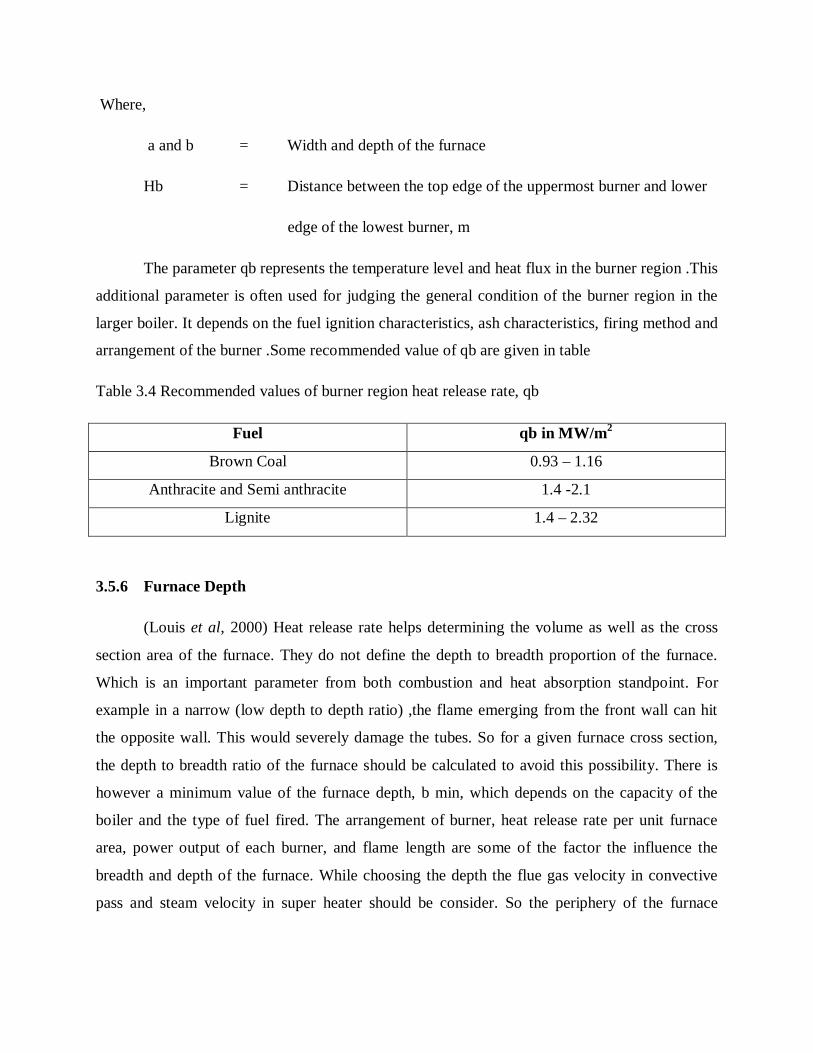
Where,

a and b = Width and depth of the furnace

Hb = Distance between the top edge of the uppermost burner and lower

edge of the lowest burner, m

The parameter qb represents the temperature level and heat flux in the burner region .This

additional parameter is often used for judging the general condition of the burner region in the

larger boiler. It depends on the fuel ignition characteristics, ash characteristics, firing method and

arrangement of the burner .Some recommended value of qb are given in table

Table 3.4 Recommended values of burner region heat release rate, qb

Fuel qb in MW/m2

Brown Coal 0.93 – 1.16

Anthracite and Semi anthracite 1.4 -2.1

Lignite 1.4 – 2.32

3.5.6 Furnace Depth

(Louis et al, 2000) Heat release rate helps determining the volume as well as the cross

section area of the furnace. They do not define the depth to breadth proportion of the furnace.

Which is an important parameter from both combustion and heat absorption standpoint. For

example in a narrow (low depth to depth ratio) ,the flame emerging from the front wall can hit

the opposite wall. This would severely damage the tubes. So for a given furnace cross section,

the depth to breadth ratio of the furnace should be calculated to avoid this possibility. There is

however a minimum value of the furnace depth, b min, which depends on the capacity of the

boiler and the type of fuel fired. The arrangement of burner, heat release rate per unit furnace

area, power output of each burner, and flame length are some of the factor the influence the

breadth and depth of the furnace. While choosing the depth the flue gas velocity in convective

pass and steam velocity in super heater should be consider. So the periphery of the furnace

should also consider the steam –water velocity through these tubes. It is essential important for

boiler pressure above 9.8 MPa.

3.5.7 Furnace Height

The furnace should be sufficiently high so that the flame does not hit the super heater

tubes. Height must exceed the minimum value, depending on the type of fuel used and capacity

of the boiler. The shorter the furnace height, the worse the natural circulation. Thus a minimum

furnace height also needed for the required degree of natural circulation(Louis et al, 2000).

3.5.8 Furnace Exit Gas Temperature

The furnace exit gas temperature (FEGT) is the important design parameter. It defines the

ratio of heat absorption by the radiant heating surface in the furnace and that by the convective

heating surfaces downstream of the furnace. This parameter is governed by both technical and

economical factor. A higher FEGT would make the furnace compact but the convective section

larger (Louis et al, 2000).

3.6 Heat and Mass Transfer in Furnace

It is important to study the heat and mass transfer to understand the energy performance

of furnace. The mass flow rate of flue gas ad its temperature decides the quantity of heat transfer

by convection and mass of fuel burning decides the Radiative heat transfer to the water wall.

3.6.1 Furnace Heat Transfer

Kumar, 2009 said that Heat conductivity coefficient is a physical parameter of substance.

In general, heat conductivity coefficient depends on temperature, pressure and substance. Heat

Transfer by conduction in flue gases occurs through transport of the kinetic energy of molecular

motion resulting from the random movement and collision of the molecules. From the concept of

kinetic theory, mean travel velocity V of the gas molecules is prescribed by the relation

푉 = 3퐺푇푀

Where,

V = Velocity of gas molecule (m/s)

G = Universal Gas Constant (8.314 Kg m2 / s2 mol K)

M = Molecular weight of the gas (Kg/ mol)

T = Absolute Temperature ( o K)

Thermal Conductivity is worked from the relation

푘 = 13 푉퐶

(푙휌)

Where,

푙 = Mean free path (average distance travelled by a molecule before

experiencing collision)

퐶 = Specific Heat at constant volume

휌 = Mass Density

Experimental investigation shows that with increase in pressure within the furnace the

gas density increases; while the mean free path diminishes in the inverse proportion. However

the product (푙휌) practically remains constant there by that thermal conductivity of gases does not

depend upon the pressure. An increase in thermal conductivity of mixture of gas (flue gas) with

rise in temperature may be attributed to an increase in mean travel velocity and specific heat at

elevated temperature. The increased agitations of gaseous molecules at elevated temperature also

results in greater frequency contact and an attendant increase in molecular exchange rate.

3.6.2 Determining Heat Transfer Coefficient to the fuel particle in Fuel bed

The overall gas-side heat transfer coefficient ho can be written as a sum of the

contributions of three components: particle convection or conduction hcond, gas convection

hconv, and radiation hrad ( Vernbanck, 1977).

ℎ = ℎ + ℎ + ℎ

For a gas passing at a superficial velocity V through a fixed bed with a large number of particles,

Gas convection may be calculated using the following equations

(푁푢) = ℎ 푑퐾 = 0.05푅 푃 푅 < 2000

(푁푢) = ℎ 푑퐾 = 0.18푅 푃 푅 > 2000

Where,

푅푒푦푛표푙푑푠푁푢푚푏푒푟,푅 = 휌푣푑휇

푃푟푎푛푑푡푙푁푢푚푏푒푟,푃 = 퐶 휇/퐾

This situation is different from one in which the whole bed of particles is involved in

exchanging heat with the fluidizing gas. At a low Reynolds number, the gas–particle heat

transfer coefficient on bulk solids in the bed is lower than that on single (isolated) particles. It

can be as much as three orders of magnitude below the single-particle heat transfer coefficient.

However, in coarse-particle beds the gas–particle heat transfer coefficients for both bulk solids

and isolated particles are closer.

3.6.3 Heat Transfer to the wall of the furnace near bed

Vernbanck, 1977 said that by analyzing data from commercially-operating boilers,

practicing engineers often develop and use rough but simple correlations for overall heat transfer

to the water wall h. One such empirical relation is

ℎ = 5휌 . 푇 . 푊/푚 퐾

Where,

휌 = Average density of fuel bed in furnace

푇 = Average temperature of fuel bed

3.6.4 Gas temperature at furnace exit

The model uses the combustion heat balance equation whereby the total net heat input

into the furnace equates the sum of the heat absorbed by the furnace walls and the heat carried by

the gases leaving the furnace (Vernbanck, 1977). The model uses the ambient air temperature as

its reference temperature, therefore the net heat input into the furnace per kilogram of fuel burnt

can be written as

퐻 = 퐻푒푎푡푖푛푓푢푒푙푏푢푟푛푡 + 퐻푒푎푡푖푛ℎ표푡푐표푚푏푢푠푡푖표푛푎푖푟

= 푁퐶푉 + 푚 (푐 푡 − 푐 푡 )

Where,

퐻 = Net heat input in the furnace in kJ/kg fuel burnt

NCV = Net calorific value of the fuel in kJ/kg

푚 = Hot combustion air flow in kg/kg fuel burnt

푐 = Specific heat of the air at 푡 in kJ/kg o C

푡 = Temperature of the hot air in °C

푐 = Specific heat of the ambient air in kJ/kg OC

푡 = Ambient air temperature in o C

The heat absorbed by the surrounding walls can be defined by the corrected Stefan-Boltzmann

equation and thus the following equation can be written

퐻 = 퐻푒푎푡푎푏푠표푟푏푒푑푏푦푓푖푟푛푎푐푒푤푎푙푙 + 퐻푒푎푐푎푟푟푖푒푑푏푦푡ℎ푒푔푎푠푙푒푎푣푖푛푔푡ℎ푒푓푢푟푛푎푐푒

= 20.53.퐹푟.퐵퐵푆퐴

푚 푇

100 ^4 −푇

100 ^4 + 푚 (푐 푡 −푐 푡 )

Where,

20.53 = Stefan-Boltzmann constant in kJ/h m2 °K4

Fr = correction factor for geometry and emissivity

(Dimensionless); (0.72 for wood)

BBSA = Total effective black body surface area of the furnace

in m2

푚 = Amount of fuel burnt in kg/h

푇 = Absolute temperature of the exit gas in o K

푇 = Absolute temperature of the furnace walls in o K

푚 = Mass of flue gas produced per kg fuel burnt in kg/kg

푐 = Specific heat of the gas at temperature t, in kJ/kg o C

푡 = Exit gas temperature in °C.

3.6.5 Determining flue gas property

Molar specific heats Cp, in kJ/(kmol K) at atmospheric pressure for various common

gases as a function of temperature ( Vernbanck, 1977) which can be determined from

퐶 = 푎 + 푏푇 + 푐푇 + 푑푇 퐾퐽/(푘푚표푙퐾)

Where,

T = Gas Temperature in o K

Value a,b,c and d are given in Annexure D.

3.6.6 Thermal Conductivity of flue gas

The thermal conductivity of the flue gas can be determined by the formula (Vernbanck, 1977).

퐾 = 퐾 × 푟 × 푍 × 1.085

Where,

퐾 = Thermal conductivity of the flue gas in W/moC

퐾 = Thermal conductivity of the flue gas component in W/moC

푟 = Volumetric fraction of the component in m3/m3

Z = 1 + 0.402푦 . (1− 푦)

y = Volumetric fraction of H20 in m3/m3

The volumetric fraction of the component is determined from the mass fraction of the

component, from:

푟 = 푚 × 푅푅

Where,

푟 = Volumetricfractionofthecomponentinm3/m3

푚 = Mass fraction of the component in kg/kg

푅 = Gas constant of the component in Nmlkg °C

RC0 2 = 188; R02 = 260; RH2 =4120; RS02 =130

RN2 = 297; RH20 = 462

푅 = Gas constant of flue gas Nm/KgoC

=푆푚 × 푅

푚 = Mass fraction of flue gas component in kg/kg

3.6.7 Determining Dynamic Viscosity of flue gas

Vernbanck, 1977 said that the dynamic viscosity of the flue gas can be determined from

휇 = ∑ 휇 .푚 / 푀∑푚 / 푀

Where,

휇 = Dynamic viscosity of flue gas in kg/ms

휇 = Dynamic viscosity of flue gas component in kg/ms

푀 = Molecular mass of flue gas component in kg/ kmol

3.6.8 Determining Non-luminous radiative coefficient

The presence of water vapour and carbon dioxide in the flue gas is important in boiler

calculations. They are selective radiators that both emit and absorb radiation in certain

wavelengths that are not visible, hence the term non-luminous. The nonluminous radiation is

dependent on gas temperature, the partial pressure of the gaseous constituents and the geometry.

The non-luminous coefficient can be calculated as shown below.

ℎ = ℎ × 퐾 × 퐾

Where,

ℎ = 4.1868푃

⎣⎢⎢⎢⎡푡 + 71.5 − 28.5

ln( 푥0.015625)푙푛2

1271.5− 28.5ln( 푥

0.015625)푙푛2 ⎦

⎥⎥⎥⎤퐾퐽/푚 ℎ 퐶

ℎ = Radiation coefficient in KJ/m2h °C

푡 = Gas temperature in °C

x = MBL X [PH (Pc + PH)]0.5

MBL = Mean beam length in m

PH = Partial pressure of H20

PC = Partial pressure of CO2

PX = ao + a1x + a2 x2 +a3 x3 + a4 x4+a5 x5

With:

ao = 10248755 a1 = 2590015

a2 = -5214298 a3 = 5838360

a4 = -3038581 a5 = 58109

Kt = Temperature correction factor

Where,

퐾 = × for wall temperature < 300 oC

= (0.73 × 푘 − 0.719) × ( ) .+ 1 for wall temperature between 300 & 600oC

Tg = Log mean temperature of gas in oK

Tw = Log mean wall temperature in oK

KE = Wall emissivity correction factor (taken = 1)

For the boiler model calculation, the total gas pressure can be considered to be

atmospheric. Hence, the partial pressures of the H20 and CO2 components can be taken equal to

their volumetric fractions (Vernbanck, 1977).

3.6.9 Determining Convective coefficient for cross flow

The convective coefficient for gas flow across a bundle of tubes on wall can be determined from

푁 = 퐾.푅 . 푃 .

or

ℎ = 퐾.퐷 . .퐺 . . 푐 . .휇 . .퐾 .

Where,

ℎ = Convective coefficient in W/m2 o C

K = 0.287 for in-line tube arrangement

= 0.32 for staggered tube arrangement

D = Outside diameter of tube in m

G = Flue gas mass flux in kg/m2s

c = Specific heat of flue gas in J/kg o C

µ = Dynamic viscosity of flue gas in kg/ms

k = Thermal conductivity of flue gas in W/m o C.

The properties of the flue gas are in this case determined for the film temperature, defined as

follows

푡 = 푡 + 푡

2

Where,

푡 = Film temperature in o C

푡 = Log mean wall temperature in o C

푡 = Log mean gas temperature in o C.

The formula is valid for turbulent flow with a Reynolds number greater than 2000 and for

tube banks at least 10 rows deep. An arrangement factor has to be applied to the result to adjust

for the geometry of the bank. This factor is dependent on the ratio between longitudinal, as well

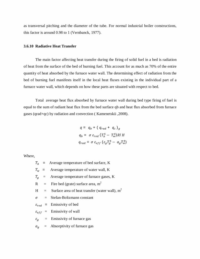
as transversal pitching and the diameter of the tube. For normal industrial boiler constructions,

this factor is around 0.98 to 1 (Vernbanck, 1977).

3.6.10 Radiative Heat Transfer

The main factor affecting heat transfer during the firing of solid fuel in a bed is radiation

of heat from the surface of the bed of burning fuel. This account for as much as 70% of the entire

quantity of heat absorbed by the furnace water wall. The determining effect of radiation from the

bed of burning fuel manifests itself in the local heat fluxes existing in the individual part of a

furnace water wall, which depends on how these parts are situated with respect to bed.

Total average heat flux absorbed by furnace water wall during bed type firing of fuel is

equal to the sum of radiant heat flux from the bed surface qb and heat flux absorbed from furnace

gases (qrad+qc) by radiation and convection ( Kamenetskii ,2008).

푞 = 푞 + (푞 + 푞 )

푞 = 휎휀 (푇 −푇 )푅/퐻

푞 = 휎휀 (휀 푇 −푎 푇 )

Where,

푇 =Average temperature of bed surface, K

푇 = Average temperature of water wall, K

푇 = Average temperature of furnace gases, K

R = Fire bed (grate) surface area, m2

H = Surface area of heat transfer (water wall), m2

휎 = Stefan-Boltzmann constant

휀 = Emissivity of bed

휀 = Emissivity of wall

휀 = Emissivity of furnace gas

푎 = Absorptivity of furnace gas

3.6.11 Mass Transfer

The mass balance of combustion air supplied and resultant combustion product can be

useful tool to quantify the energy transfer associated with the combustion products that evolved

in the furnace (D.S.Kumar, 2009)

The mass transfer operations can be classified in to the following categories;

(i) Diffusion mass transfer; molecular or eddy diffusion

(ii) Convective mass transfer: free or forced

(iii) Mass transfer by change of phase

Inside the furnace the mass transfer of gases are occurring through diffusion and convective mass

transfer. So we are not taken in to account of phase change mechanism.

3.6.12 Diffusion mass transfer; molecular or eddy diffusion

The molecular diffusion is the transport of matter on a microscopic level as a result of

diffusion from a region of high concentration in a system of a mixture of liquid or gases. The

diffusion mas transfer occurs when a substance diffuses through a layer of stagnant fluid. It is

independent of any convection within the system ( D.S.Kumar, 2009).

The molecular diffusion is further categorized in to;

- Ordinary diffusion resulting from concentration gradient; the diffusing substance moves

from a position of high concentration to one of low concentration.

- Thermal diffusion which may occur by virtue of temperature gradient

- Pressure diffusion resulting from hydrostatic pressure difference that provides the driving

potential

- Forces diffusion which results from the action of external forces

The eddy diffusion occurs when one of the diffusing fluids is in turbulent motion. The

eddying motion greatly increases the speed of the mass transfer as it is in additional to

molecular diffusion.

3.6.13 Convective mass transfer: free or forced

Mass transfer due to convection involves transfer between a moving fluid and a surface

or between two relatively immiscible moving fluids. The convective mass transfer depends both

on the transport properties and on the dynamic (laminar or turbulent) characteristics of the

flowing fluid.

3.6.14 Determining Velocity, concentration and flux of flue gas mixture

Some of the terms associated with different species in a multi-component mixture are

defined below for better understanding of the phenomenon of mass transfer (D.S.Kumar,2009).

3.6.14.1 Concentrations

The mass concentration or mass density 휌 of species A in a multicomponent mixture is

defined as the mass of species A per unit volume of the mixture.

휌 = 푚푎푠푠표푓푠푝푒푐푖푒푠퐴

푉표푙푢푚푒표푓푡ℎ푒푚푖푥푡푢푟푒

The mass concentration is quite often represented by the symbol C also. In that case 휌 = 퐶

The molar concentration or molar density represents the number of moles of species A per unit

volume of the mixture.

푛 = 푛푢푚푏푒푟표푓푚표푙푒푐푢푙푒푠표푓푠푝푒푐푖푒푠퐴

푉표푙푢푚푒표푓푡ℎ푒푚푖푥푡푢푟푒

Since the number of moles equal the mass divided by the molecular weight,

푛 = 푚푎푠푠표푓푠푝푒푐푖푒푠퐴

푉표푙푢푚푒표푓푡ℎ푒푚푖푥푡푢푟푒 × 1

푚표푙.푤푡.표푓푠푝푒푐푖푒푠퐴 = 휌푀

The mass fraction 휌∗ prescribes the ratio of mass concentration of species A to the total mass

density of the mixture

휌∗ =휌휌 =

퐶퐶

The mole fraction 푛∗ prescribes the ratio of number of moles of species A to the total number of

moles of the mixture.

푛∗ = 푛

푛 + 푛 = 푛푛

Where n is the molar density of the mixture, i.e., number of moles in the mixture per unit volume

By summation of fraction overs species,

휌∗ = 휌∗ + 휌∗

= 휌휌 +

휌휌 =

휌 + 휌휌 = 1

and

푛∗ = 푛∗ + 푛∗

= 푛푛 +

푛푛 =

푛 + 푛푛 = 1

Further,

푀 = 휌푛 =

휌 + 휌푛

= 푛 푀 + 푛 푀

푛

= 푛∗푀 + 푛∗ 푀

Thus the molecular weight of the mixture can be worked out by adding the molecular weights of

the individual species in proportion to their mole fractions.

For a gaseous phase, the concentrations are usually expressed in term of partial pressures.

Invoking the perfect gas law,

푝 푉 = 푁 퐺푇

The molar concentration is

푛 = 푁 푉 =

휌퐺푇

Where,

휌 = Pressure of species A

푁 = Total number of moles of species A in the volume V

T = Absolute temperature

G = Universal Gas Constant (G = 8314 Nm /Kg mol K)

Likewise the mole fraction for ideal gas is

푛∗ = 푛 푛 =

푝퐺푇

푝퐺푇

= 푝푝

Where,

푝 = Total pressure exerted by the gas mixture; 푝 = 푝 + 푝

3.6.14.2 Velocities

Each component/species of a multi – component mixture has a different mobility rate and

the bulk velocity of the mixture is computed either on mass – average or molar – average basis.

For a binary mixture of species A and B,

The mass-average velocity V mass is defined as

푉 = 휌 푉 + 휌 푉휌 + 휌

= 휌 푉 + 휌 푉

휌 = 휌∗푉 + 휌∗푉

The molar – average velocity V molar is defined as

푉 = 푛 푉 + 푛 푉푛 + 푛

=푛 푉 + 푛 푉

푛 = 푛∗푉 + 푛∗푉

3.6.14.3 Fluxes

The existence of different velocities and concentration causes flux of mass transfer. For

species A of the multi – component mixture,

Absolute flux = 휌 푉

Bulk motion flux = 휌 푉푚푎푠푠

Diffusion flux =

The quantity 푚푎퐴 represents mass flow per unit time.

The absolute flux of any constituent as seen by a stationary observer equals the sum of diffusion

flux and the bulk motion flux. That is,

휌 푉 = + 휌 푉

Accordingly the diffusion flux is,

푚퐴 = 휌 (푉 −푉 )

The diffusion flux is thus proportional to the difference is the velocity of component and the bulk

velocity. This velocity difference is called the diffusion velocity.

Therefore Mass-diffusion velocity of species A = 푉 −푉

Similarly on molar basis;

Molar-diffusion velocity = 푉 −푉

Diffusion flux = 푛 (푉 −푉 )

3.7 Determining Pressure drop across bed of fuel in grate

A fixed or packed bed refers to a bed of stationary particles residing on a perforated grid,

through which a gas flows. Here, the particles do not move relative to each other. When the gas

flows through a packed bed of solids it exerts a drag force on the particles, causing a pressure

drop across the bed. The pressure drop per unit height of a packed bed, ΔP/L of uniformly sized

particles, dp is correlated as (Prabir, 2006)

∆푃퐿 = 150

(1 − 휀)휀

휇푈(∅푑 ) + 1.75

(1− 휀)휀

휌 푈∅푑

Where

∆ = N/푚 permeteroffuelbeddepth

휀= Void fraction in the bed

∅ = Sphericity of bed solids

휇 = Dynamic Viscosity of gas, Kg/m s

휌 = Density of gas, Kg/m3

U = Gas flow rate per unit cross section of the bed, m/s

Results and Discussion

CHAPTER IV

RESULTS AND DISCUSSION

The results obtain from the model study on biomass burning rate, particle burning time,

heat release from fuel bed, flue gas property, convective and radiative heat transfer, flue gas exit

temperature and pressure drop across fuel bed are given in this chapter under the following major

subheadings. The discussions made on the results in the study are also presented here.

4.1 Selected boiler design

4.2 Biomass burning rate

4.3 Particle burning time

4.4 Heat Release Rate per unit volume (qv)

4.5 Heat Release Rate per Unit Cross Sectional Area (qF)

4.6 Flue Gas molecular Velocity

4.7 Stoichiometric air requirement for combustion

4.8 Property of flue gas

4.9 Heat release from fuel bed

4.10 Determining furnace wall temperature for selected boiler design

4.11 Non- Luminous Radiative Coefficient

4.12 Convective coefficient for cross flow

4.13 Determining internal heat transfer coefficient

4.14 Determining heat transfer to cavity wall

4.15 Radiative heat transfer

4.16 Pressure Drop across fuel bed

4.1 Selected boiler design

The steam Generator mainly consists of furnace, super heater, boiler bank, economizer

and air heater

4.1.1 Grate

Bio-mass is fed into furnace with the help of mechanical or pneumatic fuel feeders and

spreaders. Fuel burns on firing grate generating heat. Some of the fuel is burnt as soon as it

enters the furnace in air and is called suspension firing. This heat is absorbed by various boiler

heat transfer sections and used to convert water into steam. Depending up on the fuel type and

it's characteristics, a suitable grate is selected for firing purpose. There are various types of

Grates available like Travelling grate, chain grate, inclined water cooled grate, pin hole grate,

dumping grate, fixed grate..etc. Travelling Grate is widely used for high ash content fuels and

medium range boilers and traveling grate design is used in this study.

4.1.2 Furnace

Furnace is usually vertical and water tube type (Fig.4.1). Furnace water walls are either

membrane wall type or tangent tube wall or space tube type. Furnace absorbs major portion of

the heat generated during fuel combustion through radiation heat transfer. Proper residence time

is selected during furnace design in order to ensure that the fuel gets enough time to burn

completely inside the furnace. Boiler furnace parts include furnace bottom headers and top

headers on four walls connected with furnace wall tubes which absorb radiation in the furnace.

Headers are usually made up of carbon steel pipes and tubes are also of carbon steel. Furnace has

a provision for secondary air, fuel feeders. Furnace headers are connected to down comer pipes

from Lower drum (water drum). Furnace top headers are connected to Steam/water drum or Top

drum with the help of riser tubes/pipes thus completing the circuit. So water from lower drum

enters the furnace lower headers and then passes through furnace tubes absorbing heat. Part of

the water converts to steam on account of heat absorption and this two phase water/steam enters

furnace top headers. This steam and water mixture then enters Steam Drum through risers thus

completing the circuit. This process is called circulation and the term to describe this water to

steam ratio is called circulation ratio. In water tube boiler furnaces this ratio ranges from 15 to 25

in the case of natural circulation boilers. In assisted circulation or forced circulation boilers,

Fig. 4.1 Furnace different level

Fig. 4.2 Two stage superheater - Primary and Secondary

steam water mixture is circulated with the help of a pump unlike natural circulation boiler where

it happens because of density difference between steam and water. So forced circulation is

required for only high pressure boilers above 150 bar or so and the circulation ratio is much

lower and less than 10. In single drum boilers, the furnace is made very tall to absorb the

additional heat load required because of the absence of the boiler bank.

4.1.3 Boiler Bank

Boiler bank absorbs heat from hot gases through convection (Fig.4.3). Usually Boiler

bank is bulky as it has to absorb heat by convection at relatively low temperature. Most of the

grate fired boilers are of Bi-Drum construction where the lower drum is always filled with the

water and the upper drum is half full with water and the rest with steam. Both the drum are

connected by hundreds of tubes and sometimes thousands of tubes. Material of construction is

carbon steel for both the drums and tubes. Now-a-days single drum boilers are gaining popularity

as this expensive boiler bank can be avoided. Rotary soot blowers are provided to dust-off the

soot.

4.1.4 Superheater

Superheater is the prime section in any boiler (Fig. 4.2). Right design of the superheater

is very critical in the boiler. Superheater absorbs heat by direct radiation from furnace, by non-

luminous radiation and by convection. Superheater section is generally protected by furnace nose

in many industrial boilers. some superheaters, called platten type, kept directly hanging in the

furnace to absorb more heat. Superheater consists of Inlet outlet headers connected with

superheater coils. Inter-stage desuperheater / attemparetor is generally provided to control the

steam outlet temperature. Depending up on the steam temperature and resultant metal

temperature of the superheater coils either carbon steel or low alloy material is used.

Superheaters are also provided with steam or sonic soot soot blowers of retractable type.

4.1.5 Economizer

Economizer is used downstream of Boiler bank to preheat the feed water absorbing heat

from hot exhaust gases. Economizers are always water tube type. Bare tubes in Economizers are

widely used in Industrial boilers. Finned tubes are popular in HRSG applications. Economizers

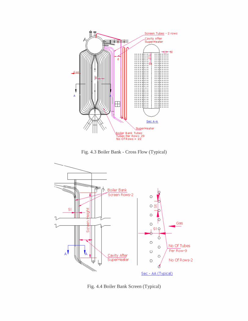
Fig. 4.3 Boiler Bank - Cross Flow (Typical)

Fig. 4.4 Boiler Bank Screen (Typical)

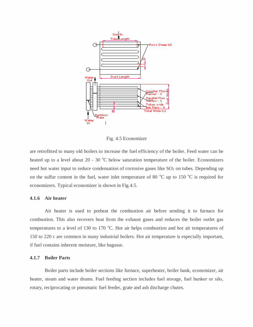
Fig. 4.5 Economizer

are retrofitted to many old boilers to increase the fuel efficiency of the boiler. Feed water can be

heated up to a level about 20 - 30 oC below saturation temperature of the boiler. Economizers

need hot water input to reduce condensation of corrosive gases like SO2 on tubes. Depending up

on the sulfur content in the fuel, water inlet temperature of 80 oC up to 150 oC is required for

economizers. Typical economizer is shown in Fig.4.5.

4.1.6 Air heater

Air heater is used to preheat the combustion air before sending it to furnace for

combustion. This also recovers heat from the exhaust gases and reduces the boiler outlet gas

temperatures to a level of 130 to 170 oC. Hot air helps combustion and hot air temperatures of

150 to 220 c are common in many industrial boilers. Hot air temperature is especially important,

if fuel contains inherent moisture, like bagasse.

4.1.7 Boiler Parts

Boiler parts include boiler sections like furnace, superheater, boiler bank, economizer, air

heater, steam and water drums. Fuel feeding section includes fuel storage, fuel bunker or silo,

rotary, reciprocating or pneumatic fuel feeder, grate and ash discharge chutes.

4.1.8 Highlighted design parameters of selected boiler

The main design parameters of the boiler are discussed here. Detail design of the boiler

components are produced in annexure.

4.1.8.a Boiler Rating

Steam Capacity (Actual) : 80 TPH

Steam Pressure (g) : 65 Kg/Cm2

Steam Outlet temperature : 485 Deg C

Water inlet temperature : 105 Deg C

Grate Type : Travelling

Furnace : Nose type

Furnace Wall : Membrane

Super Heater : Two Stages – Primary Counter, Secondary Parallel

Boiler Bank : Water Tube

Boiler Bank Flow : Cross Flow

Fuel Name : Wood

4.1.8.b Performance Detail

Efficiency(GCV) : 83.46

Efficiency(NCV) : 89.27

Gross Cal Value : 3,985.88 Kcal/Kg

Net Cal Value : 3,726.49 Kcal/Kg

Fuel Sensible Heat : 0.00 Kcal/Kg

Fuel Consumption : 17,054.88 Kg/hr

Gross Heat Input : 6.798 × 107 Kcal/ hr

Net Heat Input : 6.355×107 Kcal/ hr

Total Heat Load : 5.673×107 Kcal/ hr

Gas Flow : 1.290×105 Kg/ hr

FGR Flow : 0.000

Total DraftLoss(Gas) : 7.749X10 mm of WC

Boiler Heating Surface Area : 3,983.62 m2

4.1.8.c Furnace

Exit Gas Temp : 996.11 Deg C

Eff Proj Rad Surface(EPRS): 317.12 m2

Volumetric Heat Rel Rate : 192,926.44 Kcal/m3

Further design parameters and working parameters of primary, secondary super heaters,

boiler drum, boiler bank, boiler bank screen, economizer and air preheater are produced in

Annexure E which is designed using FIRE CAD Tool.

4.2 Biomass burning rate

Generally the biomass which are less than < 5 cm are used in boiler. The biomass size

more than these size will result in poor and prolonged combustion. For our study purpose the

wood aspects are iterated by starting with size equals 5cm diameter and then less.

Wood diameter = 5 Cm

Wood piece Length = 6 Cm

Particle temperature = 1800 K

Kinetic Rate constant ,Kc = 13.9 m/s

Assume molecular weight of gases at surface = 30 Kg / Kmol

Assume wood are in cylindrical shape

Volume of wood single piece = 휋푟 ℎ

=3.14 × 0.025 × 0.06

= 1.17× 10 푚

Surface area of wood piece = 2휋푟ℎ

= 2 × 3.14× 0.025× 0.06

= 9.42× 10 푚

Volume diameter (dv)

푑 = [6휋 × 푉표푙푢푚푒표푓푝푎푟푡푖푐푙푒]

= [ × 1.17 × 10 ]

= 0.060 m3

Surface diameter (ds)

푑 = [푆푢푟푓푎푐푒푎푟푒푎표푓푝푎푟푡푖푐푙푒

휋 ]

= [9.42× 10

휋 ]

= 0.0547푚

Sphericity (Ø)

푆푝ℎ푒푟푖푐푖푡푦(∅) = 푆푢푟푓푎푐푒푎푟푒푎표푓푎푠푝ℎ푒푟푒푤푖푡ℎ푡ℎ푒푣표푙푢푚푒푠푎푚푒푎푠푡ℎ푒푝푎푟푡푖푐푙푒

퐴푐푡푢푎푙푠푢푟푓푎푐푒푎푟푒푎표푓푡ℎ푒푝푎푟푡푖푐푙푒

= 휋푑푣푆

푆푝ℎ푒푟푖푐푖푡푦(∅) = 3.14 × (0.060)

9.42× 10 = 1.2

Spherical particle has a sphericity = 1

Since the wood is chopped in to smaller pieces which merely resembles cylindrical structure .So

its sphericity value is 1.2 which shows its deviation from spherical shape.

Since the wood shape doesn’t resembles spherical structure, assuming the mean diameter of the

selected wood as 5 cm for our study iteration.

Mean diameter of wood = 5 Cm

= 5 × 10-2 m

Density of gas by ideal gas law at surface temperature, ρ =

= 1013258315

30 1800

= 0.20 Kg / m3

Mass diffusivity is estimated using a value for CO2 in N2 from Annexure C, corrected to 1800 K

퐷 = (1800퐾293퐾 ) . × 1.6× 10

푚푠

= 2.4 × 10 -4 m2/s

Assuming Yo2,S = 0 for the time being

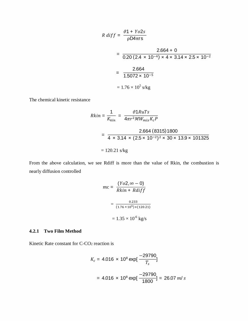
푅푑푖푓푓 = 휗1 + 푌표2푠ρD4πrs

= 2.664 + 0

0.20(2.4× 10 ) × 4 × 3.14 × 2.5 × 10

= 2.664

1.5072 × 10

= 1.76 × 105 s/kg

The chemical kinetic resistance

푅푘푖푛 =1퐾 =

휗1푅푢푇푠4휋푟 푀푊 퐾 푃

= 2.664(8315)1800

4 × 3.14× (2.5 × 10 ) × 30 × 13.9 × 101325

= 120.21 s/kg

From the above calculation, we see Rdiff is more than the value of Rkin, the combustion is

nearly diffusion controlled

푚c = (푌표2,∞− 0)푅푘푖푛 + 푅푑푖푓푓

= .( . × ) ( . )

= 1.35 × 10-6 kg/s

4.2.1 Two Film Method

Kinetic Rate constant for C-CO2 reaction is

퐾 = 4.016× 10 exp[−29790

푇 ]

= 4.016× 10 exp[−29790

1800 ] = 26.07푚/푠

The combustion rate can be expressed in term of surface CO2 Concentration

푚 = 4휋푟 퐾 푀푊 푀푊푀푊

푃푅 푇 푌 ,

= 4 × 3.14 × (2.5 × 10 ) × 26.07 × 12 × 30 × 101325

44.01 × 8315 × 1800

= 0.01133푌 , 퐾푔푠

Another equation which governs the burning rate is

푚 = 4휋푟 휌퐷ln(1 + 퐵)

= 4 × 3.14 × (2.5 × 10 ) × 0.2 × 1.57 × 10 ln(1 + 퐵)

= 9.85 × 10 ln(1 + 퐵)

퐵 =2푌표2훼 − 휗 − 1

휗 푌푐표2, 푠

휗 − 1 + (휗 − 1)휗 푌푐표2, 푠

= ( . ) .

.

. .. ,

= 0.466− 0.727푌푐표2,푠2.664 + 0.727푌푐표2,푠

Solving equation a,b,c iteratively. We start the iteration assuming YCO2,s is zero, the diffusion

controlled limit.

Table 4.1 shows the iteration results of two film model

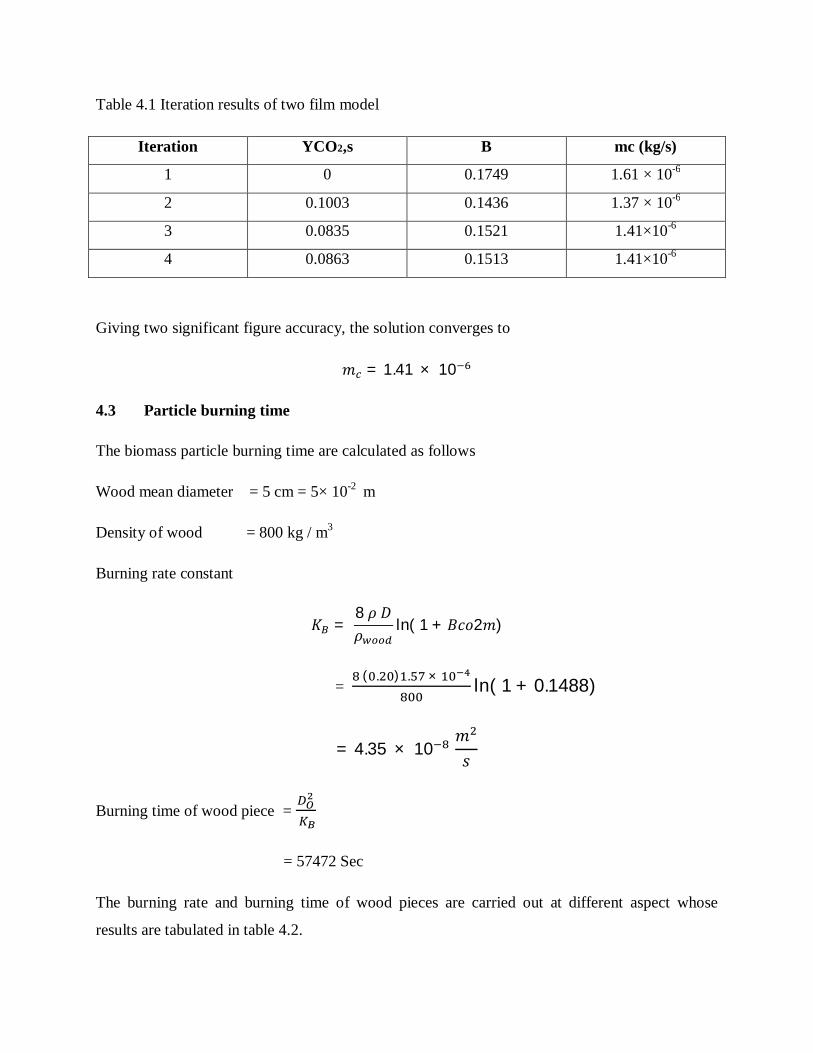
Table 4.1 Iteration results of two film model

Iteration YCO2,s B mc (kg/s)

1 0 0.1749 1.61 × 10-6

2 0.1003 0.1436 1.37 × 10-6

3 0.0835 0.1521 1.41×10-6

4 0.0863 0.1513 1.41×10-6

Giving two significant figure accuracy, the solution converges to

푚 = 1.41× 10

4.3 Particle burning time

The biomass particle burning time are calculated as follows

Wood mean diameter = 5 cm = 5× 10-2 m

Density of wood = 800 kg / m3

Burning rate constant

퐾 = 8휌퐷휌 ln(1 + 퐵푐표2푚)

= ( . ) . × ln(1 + 0.1488)

= 4.35 × 10 푚푠

Burning time of wood piece =

= 57472 Sec

The burning rate and burning time of wood pieces are carried out at different aspect whose

results are tabulated in table 4.2.

Table 4.2 Burning rate and burning time of different wood piece size

Mean diameter of

wood

Burning Rate, mc (Kg/s) Burning Time

One film model Two film model

5 cm 1.35 × 10-6 1.42 × 10-6 15.37 Hrs

4 cm 1.086 × 10-6 1.13 × 10-6 9.8 Hrs

3 cm 0.81 × 10-6 0.85 × 10-6 5.5 Hrs

2 cm 0.54 × 10-6 0.56 × 10-6 2.4 Hrs

1 cm 0.27 × 10-6 0.28 × 10-6 36.9 Minutes

5 mm 0.13 × 10-6 0.14 × 10-6 9.2 Minutes

4 mm 0.10 × 10-6 0.113 × 10-6 5.9 Minutes

3 mm 0.08 × 10-6 0.085 × 10-6 3.3 Minutes

2 mm 0.053 × 10-6 0.056 × 10-6 1.47 Minutes

1 mm 0.026 × 10-6 0.028 × 10-6 22.14 Seconds

It’s observed from the Fig.4.6 that the burning time of wood particle will be low when its aspect

is minimum.

Fig. 4.6 Behavior of particle burning time with respect to biomass size

0

10000

20000

30000

40000

50000

60000

0 1 2 3 4 5 6

Burn

ing

pero

id (S

econ

ds)

Particle diameter ( 10 -2 m)

The burning rate will greatly depend on the pressure of primary air imparting on the biomass

particle whose behavior at different striking pressure are charted below in table 4.3.

Table 4.3 Behavior of burning rate with impinging primary air pressure

It’s observed from the result of experimenting the burning rate at various range of

primary air pressure, the burning rate increase tremendously with respect to increase in pressure.

But as the aspect of biomass reduces, the steepness of burning rate curve begins to lower. So,

both the biomass aspect and primary air pressure have its own role in deciding the burning rate

of particle which is shown in Fig.4.7.

S.No Burning rate of biomass by one film model (× 10-6 Kg/s)

Diameter of wood particle

Pressure, atm 5 cm 4 cm 2 cm 3 cm 1 cm

1 1 1.35 1.08 0.81 0.54 0.27

2 4 5.43 4.34 3.25 2.17 1.08

3 6 8.14 6.51 4.88 3.25 1.62

4 8 10.86 8.68 6.51 4.34 2.16

5 10 13.57 10.86 8.14 5.42 2.70

6 12 16.29 13.03 9.77 6.51 3.24

7 14 19.01 15.20 11.40 7.59 3.79

8 16 21.72 17.37 13.03 8.68 4.33

9 18 24.44 19.55 14.65 9.76 4.87

10 20 27.15 21.72 16.28 10.85 5.41

11 22 29.87 23.89 17.91 11.93 5.95

12 26 35.30 28.24 21.17 14.10 7.04

13 28 38.02 30.41 22.80 15.11 7.58

14 30 40.73 32.58 24.43 16.27 8.12

Fig. 4.7 Variation of burning rate as the function of biomass aspect and pressure

4.4 Heat Release Rate per unit volume (qv)

The quantity of energy released per unit volume of selected boiler design is calculated as follows

푞 =퐵. 퐿퐻푉푉

퐾푊푚

Designed fuel consumption rate, B = 4.73 Kg/s

Furnace Volume, V = 4.48 m × 6.73 m × 12.08 m

= 364 .21 m3

Lower Heating Value of fuel, LHV = 15592 KJ/Kg

푞 =4.73× 15592

364.21 퐾푊푚

푞 = 202.49퐾푊푚

0

5

10

15

20

25

30

35

40

45

0 5 10 15 20 25 30 35

Burn

ing

rate

by

one

film

mod

el (

10 -6

Kg

/ s )

Pressure , atm

5 cm dia

4 cm dia

3 cm dia

2 cm dia

1 cm dia

4.5 Heat Release Rate per Unit Cross Sectional Area (qF)

The quantity of energy released from unit area of fuel bed is calculated as follows

푞 = 퐵.퐿퐻푉퐹 퐾푊 푚

Cross sectional area of the furnace grate, F = 6.73 × 4.48 m2

푞 = 4.73 × 155926.73× 4.48 퐾푊 푚

푞 = 2446 퐾푊 푚

4.6 Flue Gas molecular Velocity

The velocity of flue gas molecules and its existing velocity inside the furnace are calculated as

follows. Design velocities of boiler fluids are given in Annexure B.

Flue Gas Component Molecular Weight (Kg/Kmol)

CO2 44

N2 28

O2 32

H2O 18

Gas temperature = 1000 o C = 1273 K

Mean travel velocity by kinetic theory,

푉 = 3퐺푇푀

Where,

V = Velocity of gas molecule (m/s)

G = Universal Gas Constant (8.314 Kg m2 / s2 mol K)

M = Molecular weight of the gas (Kg/ mol)

T = Absolute Temperature ( o K)

Mean travel velocity of flue gas components

푉,퐶푂 = 3 × 8.314 × 1273

0.044

= 849.48 m/s

푉,푁 = 3 × 8.314 × 1273

0.028

= 1064.88 m/s

푉,푂 = 3 × 8.314 × 1273

0.032

= 996.10 m/s

푉,퐻 푂 = 3 × 8.314 × 1273

0.018

= 1328.13 m/s

Vmass = (0.31 × 849.48) + (0.61 × 1064.88) + (0.04 × 996.10) + (0.028 × 1328.13)

= 989.92 m/s

Actual velocity of flue gas inside the furnace is established below,

Volumetric flow rate of flue gas ( m3/s) = Furnace cross sectional area ( m2) × Velocity ( m/s )

119.60 m3/s = 30.20 m2 × Velocity

Velocity = 3.96 m/s

4.7 Stoichiometric air requirement for combustion

4.7.1 Wood Composition

Carbon : 45.6 %

Hydrogen : 4 %

Nitrogen : 0.5 %

Oxygen : 37.45 %

Sulphur : 0.07 %

Moisture : 9.33 %

Ash : 3.05 %

4.7.2 Carbon Combustion:

C+O2 =CO2

12kg C + 32 Kg O2 = 44 Kg O2

1 Kg C + 2.66 Kg CO2 = 3.6 Kg CO2

In 1 kg of fuel 0.45 kg of carbon presents

Therefore,

O2 required for carbon combustion = 2.66 × 0.45

= 1.197 Kg O2

CO2 produced as byproduct = 3.6 × 0.45

= 1.62 Kg CO2

4.7.3 Hydrogen Combustion:

2H2+O2 = 2H2O

1 kg H2 + 8 Kg O2 = 9 Kg H2O

In 1 Kg of wood 0.04 kg of hydrogen presents

O2 required for combustion of this hydrogen = 0.04 × 8

= 0.32 Kg O2

H2O Produced as byproduct = 9 × 0.04

= 0.36 Kg H2O

Since sulphur is negligible we are neglecting its combustion and we assume nitrogen reactivity is

nil at low temperature.

For 1 Kg of wood

Total O2 required = 1.197 + 0.32

= 1.517 Kg

O2 presents in the fuel = 0.37 Kg /Kg fuel

Therefore actual O2 required = 1.517 – 0.37

= 1.147 Kg

For obtaining 1 Kg of O2, amount of air required = 100/23

= 4.35 Kg

(Air by mass: 23% Oxygen, 77% Nitrogen)

For 1 Kg of fuel, air required = 4.35 × 1.147

= 4.98 Kg air

Amount of nitrogen in supplied air = 4.98 × 0.77

= 3.83 Kg N2

Amount of nitrogen in fuel = 0.5 %

Total nitrogen in byproduct = 3.83 + (0.5/100)

= 3.835 Kg N2

4.7.4 Excess Air

Let’s take excess air for wood = 30%

Stoichiometric air = 4.98 Kg

Now total air = 4.98 + (4.98 × 0.30)

= 6.47 Kg of air

Nitrogen mass in byproduct = 6.47 × 0.77

= 4.98 Kg N2

4.7.5 Summary of stoichiometric and excess air calculation

Total air required = 6.47 Kg air / Kg of fuel

Byproduct formation by burning of 1 Kg of fuel

CO2 = 1.62 Kg

H20 = 0.36 Kg

N2 = 4.98 Kg

Required actual fuel firing rate in boiler = 17055 Kg /hr

Mass flow of air = 17055 Kg/ hr × 6.47 Kg air /Kg fuel

= 110346 Kg air / hr

Mass flow rate of byproduct

CO2 = 1.62 × 17055 = 27629 Kg/hr

H2O = 0.36 × 17055 = 6140 Kg/hr

N2 = 4.98 × 17055 = 84934 Kg/hr

Table 4.4 shows the mass flow rate of flue gas for actual boiler operational condition

Table 4.4 Mass flow rate of flue gas

S.No Mass flow in combustion For unit mass of

wood

For actual fuel firing

rate (17055 Kg/hr)

1 Combustion air required (In) 6.47 Kg 110346 Kg / hr

2 CO2 (Out) 1.62 Kg 27629 Kg /hr

3 H20 (Out) 0.36 Kg 6140 Kg / hr

4 N2 (Out) 4.98 Kg 84934 Kg /hr

5 Excess O2(Out) - 5800 Kg/hr

While operation of boiler 20 % of combustion air is passed as primary air and 80 % of

remaining as secondary air. It is taken in account that, due to supply of excess air about 4 – 5%

of O2 is observed in flue gas exit.

Total mass flow of flue gas = Mass flow of CO2+H2O+N2+O2, Kg/hr

= 27629 + 6140 + 84934 +5800

= 124503 Kg/hr

The flue gas composition on the weight basis is shown in table 4.5

Table 4.5 Flue gas composition by weight basis

S.No Composition Calculation of % by weight % by weight

1. CO2 (27629/124503) × 100 22.19

2. H2O (6140 / 124503) × 100 4.93

3. N2 (4934 / 124503) × 100 68.2

4. O2 ( 5800 / 124503) × 100 4.65

4.8 Property of flue gas

It’s important to know the flue gas property which plays a basic role in heat transfer

mechanism. So the flue gas properties are calculated as follows

4.8.1 Determining molar concentration, mass density and average molecular weight of

flue gas

The average molecular weight of flue gas is independent of temperature, pressure exit in

the furnace but its proportional to percentage composition of species in flue gas. In case of mass

density and molar concentration of flue gas, it’s purely dependent factor of temperature and

pressure.

Table 4.6 The partial pressure ratio and molecular weight of flue gas species are

S.No Flue gas components Partial pressure ratio, δ Molecular Weight, MW

1. CO2 0.22 44

2. N2 0.68 28

3. O2 0.046 32

4. H2O 0.049 18

The calculation are carried out for 1037oC (1310 K) at 1 × 105 N/m2 furnace pressure.

Though slightly negative pressure is maintained inside the furnace, we are taking the

atmospheric pressure for convenient in calculation.

Molar Concentration of flue gas species are

푛 = 0.22 × 10

8314× 1310 = 2.02 × 10 퐾푔푚표푙/푚

푛 = 0.68 × 10

8314× 1310 = 6.24 × 10 퐾푔푚표푙/푚

푛 = 0.046× 10

8314× 1310 = 4.22× 10 퐾푔푚표푙/푚

푛 = 0.049 × 10

8314× 1310 = 4.49× 10 퐾푔푚표푙/푚

4.8.1.a Mass Density

휌 = 44 × 2.02× 10

= 0.0888 퐾푔 푚

휌 = 28 × 6.24 × 10

= 0.1747 퐾푔 푚

휌 = 32 × 4.22× 10

= 0.0135 퐾푔 푚

휌 = 18× 4.49× 10

= 8.082× 10 퐾푔 푚

Overall mass density 휌 = 휌 + 휌 + 휌 + 휌

= 0.0888 + 0.1747 + 0.0135 + 8.082 × 10 = 0.2850 퐾푔 푚

The mass fraction of flue gas components

휌∗ = 휌휌 =

0.08880.2850 = 0.31

휌∗ = 휌휌 =

0.17470.2850 = 0.61

휌∗ = 휌휌 =

0.01350.2850 = 0.04

휌∗ = 휌휌 =

8.08× 100.2850 = 0.028

4.8.1.b Average Molecular weight of flue gas

퐴 = ∑휑 × 푀푊

Where

퐴 =Avg molecular weight of flue gas

휑 = 푃푎푟푡푖푎푙푝푟푒푠푠푢푟푒표푓푓푙푢푒푔푎푠푠푝푒푐푖푒푠(휑 ,휑 ,휑 ,휑 )

푀푊 = 푀표푙푒푐푢푙푎푟푤푒푖푔ℎ푡표푓푓푙푢푒푔푎푠푠푝푒푐푖푒푠(푀푊 ,푀푊 ,푀푊 ,푀푊 )

퐴 = (0.22× 44) + (0.68× 28) + (0.046× 32) + (0.049× 18)

= 31.07

4.8.2 Adiabatic Flame Temperature of Wood

The adiabatic flame temperature of wood burning in air would be 1900 K. Hardly it

ranges between 1800 K to 1900 K depend deviation from equivalents ratio. The flame

temperature decreases as the equivalents ratio moves away from unity. The property of flue gas

is shown in the table 4.7.

Table 4.7 Calculated property of flue gas for selected boiler design over wide range of temperature

S.No Temperature oC

Molecular Weight

Density, Kg/m3

Enthalpy, Kcal/Kg

Specific Heat,

Kcal/Kg oC

Thermal Conductivity, Kcal/hr m oC

Viscosity, Cp

1 1700 31.24 0.1938 489.96 0.1775 0.0502 0.0612 2 1650 31.24 0.1987 473.98 0.1775 0.0494 0.0603 3 1600 31.24 0.2035 458.01 0.1773 0.0486 0.0594 4 1550 31.24 0.2083 442.05 0.1771 0.0477 0.0585 5 1500 31.24 0.2147 426.12 0.1768 0.0468 0.0575 6 1450 31.24 0.2211 410.22 0.1764 0.0464 0.0566 7 1400 31.24 0.2274 394.37 0.1759 0.0451 0.0556 8 1350 31.24 0.2339 378.56 0.1753 0.0442 0.0547 9 1300 31.24 0.2419 362.81 0.1746 0.0433 0.0537

10 1250 31.24 0.2499 347.12 0.1739 0.042 0.0526 11 1200 31.24 0.2579 331.51 0.1730 0.0413 0.0516 12 1150 31.24 0.2676 315.97 0.1721 0.0404 0.0506 13 1100 31.24 0.2772 300.53 0.1711 0.0394 0.0495 14 1050 31.24 0.2884 285.17 0.1703 0.0383 0.0484 15 1000 31.24 0.2996 269.93 0.1688 0.0373 0.0473 16 950 31.24 0.3108 254.79 0.1675 0.0360 0.0462 17 900 31.24 0.3253 239.76 0.1662 0.0352 0.0450 18 850 31.24 0.3397 224.86 0.1648 0.034 0.0438 19 800 31.24 0.3557 210.08 0.1634 0.032 0.0426 20 750 31.24 0.3710 195.45 0.1618 0.0318 0.0413 21 700 31.24 0.3910 180.95 0.1602 0.030 0.0400 22 650 31.24 0.4134 166.60 0.1583 0.028 0.0380 23 600 31.24 0.4350 152.42 0.1566 0.02819 0.0374 24 550 31.24 0.4631 138.39 0.1549 0.0264 0.0360 25 500 31.24 0.4935 124.52 0.1530 0.025 0.0345

4.9 Heat release from fuel bed

The heat release rate from biomass bed varies according to its temperature of combustion

and fuel bed density. The fuel bed density is decided by the size of the biomass i.e. fuel density

on bed is fix by the void fraction of biomass which is again the factor of size and the temperature

of combustion will be nearly equals to adiabatic flame temperature, but this temperature exist

only at fuel bed not at furnace wall because of heat loss from furnace surface.

Adiabatic temperature of wood = 1900 K (1627 o C)

Density of wood = 800 Kg / m3

Void fraction exits in fuel bed, ε = 0.87

Density of fuel bed at this void fraction = 700 Kg / m3

Heat release rate from fuel bed, ℎ = 5휌 . 푇 . 푊/푚 퐾

= 5× 700 0.391 × 1900 0.408

= 87.94 푊/푚 퐾

It’s impossible to say that the fuel bed will always retain the temperature near Adiabatic

Flame Temperature (AFT). As it varies according to heat loss to surrounding, the heat release

rate from bed is carries out at different temperatures deviate from AFT (Table 4.8).

Table 4.8 Fuel bed temperature Vs. Fuel bed heat release rate.

S.No Temperature of Bed Heat release from bed (W/m2 K)

1 1900 K 1627 o C 87.94

2 1850 K 1577 o C 87.84

3 1800 K 1527 o C 87.74

4 1700 K 1427 o C 87.54

5 1500 K 1227 o C 87.09

6 1300 K 1027 o C 86.59

7 1200 K 927 o C 86.30

From Fig.4.8 that over wide temperature difference between the fuel bed (i.e. 1900 K to 1200 K)

,the heat release rate from bed doesn’t vary greatly. So the only deciding factor of heat release

rate from fuel bed is average fuel bed density which depends on void fraction or size of fuel

selected. To study this phenomenon, calculations are carried out at different fuel bed density at

AFT whose results are tabulated in table 4.9.

Table 4.9 Fuel bed density Vs. Heat release rate

S.No Fuel bed density ,Kg/m3 Heat release from bed ( W/m2 K)

1 800 92.8

2 750 90.55

3 700 88.14

4 650 85.62

5 600 82.98

6 550 80.20

7 500 77.27

Fig.4.9 shows that as the fuel density goes down, the heat release rate also goes down

proportionally. So the particle size plays the key role in deciding heat rate from fuel bed. But as

the combustion proceed, the size of biomass piece starts shrinking. So the void fraction will

change which keeps the density of fuel bed vary .To maintain the density nearly constant in the

bed, the vibrating reciprocating system is provided in the furnace grate.

4.10 Determining furnace wall temperature for selected boiler design

It’s known from the selected boiler design that the exit gas temperature of furnace is

996.11 o C which can be used in FEGT energy balance equation of furnace to determine the

furnace wall temperature.

NCV of fuel = 3726.49 Kcal / kg

= 15592 KJ / Kg

푚 = 6.47 kg /kg of fuel

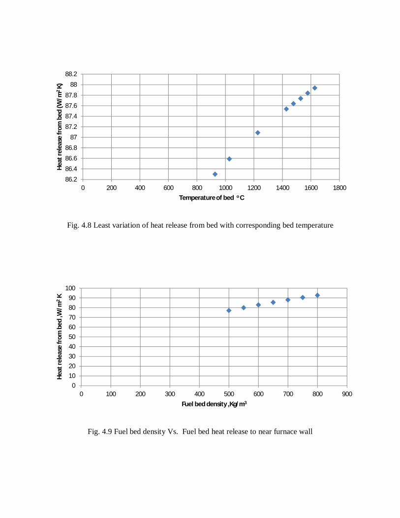
Fig. 4.8 Least variation of heat release from bed with corresponding bed temperature

Fig. 4.9 Fuel bed density Vs. Fuel bed heat release to near furnace wall

86.2

86.4

86.6

86.8

87

87.2

87.4

87.6

87.8

88

88.2

0 200 400 600 800 1000 1200 1400 1600 1800

Hea

t rel

ease

from

bed

(W/m

2 K)

Temperature of bed o C

0102030405060708090

100

0 100 200 300 400 500 600 700 800 900

Hea

t rel

ease

from

bed

,W/m

2 K

Fuel bed density ,Kg/m3

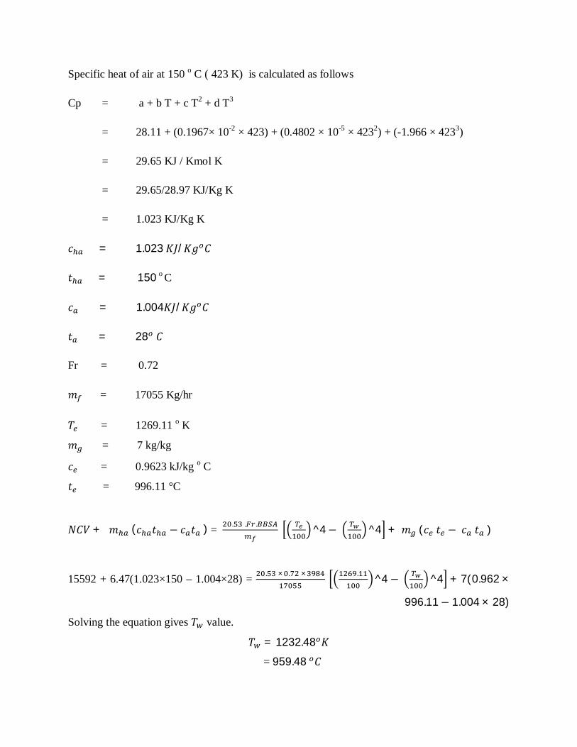
Specific heat of air at 150 o C ( 423 K) is calculated as follows

Cp = a + b T + c T2 + d T3

= 28.11 + (0.1967× 10-2 × 423) + (0.4802 × 10-5 × 4232) + (-1.966 × 4233)

= 29.65 KJ / Kmol K

= 29.65/28.97 KJ/Kg K

= 1.023 KJ/Kg K

푐 = 1.023퐾퐽/퐾푔 퐶

푡 = 150o C

푐 = 1.004퐾퐽/퐾푔 퐶

푡 = 28 퐶

Fr = 0.72

푚 = 17055 Kg/hr

푇 = 1269.11 o K

푚 = 7 kg/kg

푐 = 0.9623 kJ/kg o C

푡 = 996.11 °C

푁퐶푉 + 푚 (푐 푡 − 푐 푡 )= . . . ^4− ^4 + 푚 (푐 푡 −푐 푡 )

15592 + 6.47(1.023×150 – 1.004×28) = . × . × . ^4 − ^4 + 7(0.962 ×

996.11− 1.004 × 28)

Solving the equation gives 푇 value.

푇 = 1232.48 퐾

= 959.48 퐶

4.11 Non- Luminous Radiative Coefficient

The Non-luminous coefficient of flue gas is calculated as follows

Fluegastemperaturein°C, 푡 = 996.11 퐶

Mean Beam Length (MBL) calculation

MBL for selected boiler dimension can be obtain by choosing the appropriate dimension ratio

from table 4.10.

Table 4.10 Mean Beam Length for furnace dimension

S.no Dimensional Ratio (length, width, height in any ratio)

Mean Beam Length(MBL) ,L (m)

Rectangular Furnace

1 1-1-1 to 1-1-3

1-2-1 to 1-2-4

2/3 × (Furnace Volume) 1/3

2 1-1-4 to 1-1-infinite 1 × smallest dimension

3 1-2-5 to 1-2-8 1.3 × smallest dimension

4 1-3-3 to 1-infinite-infinite 1.8 × smallest dimension

Cylindrical furnace

5 d × d 2/3 × diameter

6 d × 2d to d× infinite 1 × diameter

Furnace geometry of selected boiler is

Depth = 4.48 m

Width = 6.73 m

Height = 12.08 m

Ratio of dimension: 1.12 – 1.68 – 3.02

Therefore, Mean Beam Length (MBL) = 2/3 (Furnace Volume) 1/3

= 2/3 (4.48 × 6.73 × 12.08) 1/3

= 4.76 m

PH = 0.049

PC = 0.22

x = MBL X [PH (Pc + PH)]0.5

= 4.76 × [0.049 (0.22 + 0.049)]0.5

PX = ao + a1x + a2 x2 +a3 x3 + a4 x4+a5 x5

= (10.24) + (259.0015 × 0.546) + (-521.4298 × 0.546 2 ) + (583.8360 ×

0.546 3) +(-303.85 × 0.546 4) + (58.10 × 0.546 5)

= 67.055

ℎ = 4.1868푃

⎣⎢⎢⎢⎡푡 + 71.5− 28.5

ln( 푥0.015625)푙푛2

1271.5− 28.5ln( 푥

0.015625)푙푛2 ⎦

⎥⎥⎥⎤퐾퐽/푚 ℎ 퐶

ℎ . = 4.1868× 67.055

⎣⎢⎢⎢⎡996.11+ 71.5 − 28.5

ln( 0.5460.015625)푙푛2

1271.5− 28.5ln( 0.546

0.015625)푙푛2 ⎦

⎥⎥⎥⎤

ℎ . = 229.877퐾퐽/푚 ℎ 퐶

Log mean temperature in oK, Tg = 1269.11 oK

Log mean wall temperature in oK, Tw = 1232.48 oK

Mean wall temperature in o C ,푡 = 959.48 퐶

퐾 = 126.11 − 1232.48

1269.11 − 573 ×996.11− 300

996.11− 959.48

= 2.186 (For wall temperature < 300 o C)

For existing wall temperature is 996.11 o C

= (0.73 × 푘 − 0.719) × ( ) .+ 1

= (0.73 × 2.186− 0.719) × ( ) .

.+ 1

= 1.00506

Taking wall emissivity correction factor = 1

ℎ = ℎ × 퐾 × 퐾

ℎ = 229.877× 1.00506× 1

= 231.88KJ/m2h °C

Non luminous Radiative coefficient is depend on flue gas temperature exist inside the

furnace. Above calculation is carried out at FEGT where there is wide gap exist between AFT

and FEGT. So let’s see the behavior of non-luminous Radiative coefficient within this

temperature range which is charted in table 4.11.

Table 4.11 Non-luminous radiative coefficient of flue gas

S.No Temperature of gas inside furnace Non-luminous Radiative coefficient

(KJ/m2h °C)

1 1627 o C 389.46

2 1500 o C 357.76

3 1400 o C 332.80

4 1300 o C 307.844

5 1200 o C 282.88

6 1100 o C 257.92

Its infer from the Fig.4.10 that there is considerable loss of non- luminous radiant coefficient

with loss in temperature from flue gas

Fig. 4.10 Variation of Non-luminous radiant coefficient with gas temperature

4.12 Convective coefficient for cross flow

The convective coefficient of membrane wall, boiler bank, boiler screen, super heaters

and economizer are calculated as follows

0

50

100

150

200

250

300

350

400

450

0 200 400 600 800 1000 1200 1400 1600 1800

Non

- lu

min

ous r

adia

tive

coef

ficie

nt

(KJ /

m2 h

o C)

Temperature of gas inside furnace , o C

4.12.1 Film temperature

The property of flue gas is determined at film temperature

Log mean wall temperature in o C , 푡 = 959.58 o C

Log mean gas temperature in o C,푡 = 1000 o C

Film temperature in o C , 푡 = .

= 980 o C

4.12.2 Flue gas mass flux

Total heating surface area of boiler = 3983.62 m2

Calculated flue gas mass flow rate is 124503 Kg/hr where fire cad design tool data is 129000

Kg/hr. So it is considered fire cad design tool data for calculation of flue gas mass flux.

Therefore, Flue gas mass flux, G = .

= 32.38

G = 8.9 × 10

4.12.3 Specific heat

Specific heat of flue gas, oC at 980 o C = 0.1688 Kcal / Kg o C

= 0.706 KJ /Kg o C

= 706 J / Kg o C

4.12.4 Thermal Conductivity

The thermal conductivity of flue gas at operating gas temperature is as follows

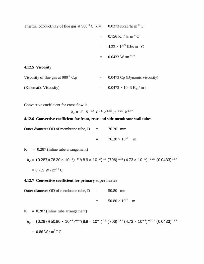
Thermal conductivity of flue gas at 980 o C, k = 0.0373 Kcal /hr m o C

= 0.156 KJ / hr m o C

= 4.33 × 10-5 KJ/s m o C

= 0.0433 W /m o C

4.12.5 Viscosity

Viscosity of flue gas at 980 o C,µ = 0.0473 Cp (Dynamic viscosity)

(Kinematic Viscosity) = 0.0473 × 10 -3 Kg / m s

Convective coefficient for cross flow is

ℎ = 퐾.퐷 . .퐺 . . 푐 . .휇 . . 푘 .

4.12.6 Convective coefficient for front, rear and side membrane wall tubes

Outer diameter OD of membrane tube, D = 76.20 mm

= 76.20 × 10-3 m

K = 0.287 (Inline tube arrangement)

ℎ = (0.287)(76.20 × 10 ) . (8.9 × 10 ) . (706) . (4.73 × 10 ) . (0.0433) .

= 0.739 W / m2 o C

4.12.7 Convective coefficient for primary super heater


= 50.80 × 10-3 m


ℎ = (0.287)(50.80 × 10 ) . (8.9 × 10 ) . (706) . (4.73 × 10 ) . (0.0433) .

= 0.86 W / m2 o C

4.12.8 Convective coefficient for secondary super heater


= 44.50 × 10 -3 m


ℎ = (0.287)(44.50 × 10 ) . (8.9 × 10 ) . (706) . (4.73 × 10 ) . (0.0433) .

= 0.9154 W / m2 o C

4.12.9 Convective coefficient for boiler bank screen


= 76.20 × 10 -3 m

K = 0.302 (Staggered tube arrangement)

ℎ = (0.302)(76.20 × 10 ) . (8.9 × 10 ) . (706) . (4.73 × 10 ) . (0.0433) .

= 0.77 W / m2 o C

4.12.10 Convective coefficient for Boiler bank


= 50.80 × 10 -3 m


ℎ = (0.287)(50.80 × 10 ) . (8.9 × 10 ) . (706) . (4.73 × 10 ) . (0.0433) .

= 0.86 W / m2 o C

4.12.11 Convective coefficient for economizer

Outer diameter OD of membrane tube, D = 50.80 mm = 50.80 × 10 -3 m


ℎ = (0.287)(50.80 × 10 ) . (8.9 × 10 ) . (706) . (4.73 × 10 ) . (0.0433) .

= 0.86 W / m2 o C

Over the range of wide temperature difference, the conductivity, viscosity and specific

heat remain constant. So the convective coefficient for cross flow highly dependent on mass flux

of flue gas and outer diameter of tube. But the outer diameter for existing boiler can’t be

changed; it has to handle at design stage itself. Here the mass flux of flue gas plays a critical role

in deciding the convective coefficient which is proportional to quantity of fuel fired.

The effect of tube diameter in convective coefficient is presented in table 4.12.

Table 4.12 Primary Super Heater tube diameter Vs. Convective Coefficient

S.No Tube OD for Primary Super Heater,

mm

(Inline arrangement)

Convective Coefficient, W/m2 o C

1 50.8 (actual OD) 0.86

2 50 0.87

3 49 0.88

4 47 0.89

5 45 0.91

6 40 0.95

7 35 1.0097

It’s observed from Fig.4.11 that with about 30 % reductions in OD of superheater, the convective

coefficient tends to increase about 15 -20 %. So these functional behaviors have to take care

while designing the OD of superheater for efficient energy transfer.

The effect of boiler fuel loading in convective coefficient is presented in table 4.13.

Table 4.13 Boiler fuel loading Vs. Convective coefficient

S.No Boiler fuel loading Mass flux of flue gas

(Kg/s m2)

Convective coefficient for

primary super heater

( W/m2 o C)

1 100% 8.9 × 10-3 0.86

2 95% 8.2 × 10-3 0.82

3 90% 7.7 × 10-3 0.79

4 85% 7.3 × 10-3 0.77

5 80% 6.9 × 10-3 0.75

6 70% 6.1 × 10-3 0.69

7 60% 5.3 × 10-3 0.63

8 50% 4.4 × 10-3 0.57

Fig.4.12 shows, till up to 80% boiler loading drop the rate of convective coefficient drop is

observed minimum. Beyond that steep fall of coefficient value is observed.

4.13 Determining internal heat transfer coefficient

ℎ = 0.023푑 . 푘 . 퐺 . 푐 . 휇 .

Thermal conductivity, k = 0.043 W/m o C

Gas mass flux, G = 8.9 ×10-3 Kg / m2s

Specific heat, c = 706 J /Kg o C

Dynamic Viscosity, µ = 4.73× 10-5 Kg/ m s

Internal heat transfer coefficient can be applicable only to super heater.

Fig. 4.11 Primary super heater tube OD vs. Convective Coefficient

Fig. 4.12 Behavior of convective coefficient with boiler fuel loading

0.84

0.86

0.88

0.9

0.92

0.94

0.96

0.98

1

1.02

0 10 20 30 40 50 60

Conv

ectiv

e Co

effic

net W

/m2

o C

Primary Super Heater tube OD,mm

0

0.1

0.2

0.3

0.4

0.5

0.6

0.7

0.8

0.9

1

0 20 40 60 80 100 120

Conv

ectiv

e Co

effic

ient

, W

/m2

o C

&

Mas

s Flu

x of

flue

gas

( ×

10-4

Kg

/ s m

2)

Boiler Fuel Loading %

Mass flux of flue gas

Convective Coefficient

4.13.1 Primary Super heater

OD = 50.80 mm

Tube thickness = 4 mm

Internal diameter, d = 50.80 – 4 = 46.8 mm

= 46.8 × 10-3 m

ℎ = 0.023(46.8× 10− 3) . (0.043) . (8.9 × 10− 3) . (706) . (4.73 × 10 − 5) .

= 0.10 W / m o C

4.13.2 Secondary Super heater

OD = 44.50 mm

Tube thickness = 4 mm

Internal diameter, d = 44.50 – 4 = 40.5 mm

= 40.5 × 10-3 m

ℎ = 0.023(40.5 × 10 − 3) . (0.043) . (8.9× 10 − 3) . (706) . (4.73 × 10− 5) .

= 0.112 W / m o C

Table 4.14 Primary Super Heater internal tube diameter Vs. Internal Heat transfer Coefficient

S.No Tube internal diameter for primary

super heater, mm

Internal heat transfer coefficient, W/m2 o C

1 46.8 (Existing) 0.108

2 45 0.109

3 44 0.110

4 43 0.110

5 42 0.111

6 40 0.112

The variation of internal heat transfer coefficient with tube internal diameter is shown in

table. It’s observed from fig that, with 15 % reduction in superheater OD, the internal heat

transfer coefficient raise only by about 3.6 %.So here it doesn’t cause much impact on heat

transfer mechanism which is shown in Fig 4.13.

The effect of boiler fuel loading in internal heat transfer coefficient is presented in table 4.15

Table 4.15 Boiler fuel loading Vs. Internal heat transfer coefficient


(Kg/s m2)

Internal heat transfer

coefficient , W/m2 o C

1 100 % 8.9 × 10-3 0.108

2 95 % 8.2 × 10-3 0.101

3 90 % 7.7 × 10-3 0.096

4 80 % 6.9 × 10-3 0.089

5 70 % 6.1 × 10-3 0.080

6 60 % 5.3 × 10-3 0.071

7 50 % 4.4 × 10-3 0.061

Here also till up to 80% boiler loading drop the rate of convective coefficient drop is

observed minimum. Beyond that steep fall of coefficient value is observed which is observed at

Fig.4.14.

4.14 Determining heat transfer to cavity wall

The heat transfer to cavity wall from flue gas is calculated as follows

Hydraulic diameter, Dh

= 4 × , ,

= 4 × . × . × = 0.36 m

Fig. 4.13 Super Heater internal diameter Vs. Internal heat transfer coefficient

Fig. 4.14 Behavior of Internal heat transfer coefficient with boiler fuel loading

0.1085

0.109

0.1095

0.11

0.1105

0.111

0.1115

0.112

0.1125

0.113

39 40 41 42 43 44 45 46 47 48

Inte

rnal

hea

t tra

nsfe

r coe

ffici

ent,W

/m2 o C

Primary Super Heater Internal diameter,mm

Flue gas mass flux, G = 32.38 Kg / hr m2

Dynamic Viscosity, µ = 4.73× 10-5 Kg/ m s

Specific heat, Cp = 0.706 KJ /Kg o C

ℎ = 0.161퐷 . 퐺 . 휇 . 푐

ℎ = 0.1610.36 . 32.38 . (4.73 × 10 − 5) . 0.706

= 0.30 KJ / h m2 o C

The effect of boiler loading on heat transfer to cavity wall is shown in table 4.16.

Table 4.16 Boiler fuel loading Vs. Heat transfer to cavity wall


(Kg / h m2)

Heat transfer to cavity wall

( KJ/h m2 o C)

1 100 % 32.38 0.30

2 95 % 29.52 0.28

3 90 % 27.72 0.27

4 85 % 26.28 0.26

5 80 % 25.09 0.25

6 70 % 21.96 0.22

7 60 % 19.11 0.20

8 50 % 15.84 0.17

Its observed that over 50% reduction in fuel loading of boiler, heat transfer to cavity wall

also drop to about 56.6% with undulation drop pattern observed in Fig.4.15.

Fig. 4.15 Boiler fuel loading vs. Heat transfer to cavity wall

4.15 Radiative heat transfer

The radiative heat transfer inside the furnace is established in following calculation, also

the convective heat transfer is included.

Average temperature of bed surface, 푇 = 1523 K (1250 o C)

Average temperature of water wall,푇 = 1232.48 K (959.48 o C)

Average temperature of furnace gases, 푇 = 1273 K (1000 o C)

Fuel bed area, R = 6.73 m × 4.48 m = 30.15 m2

Surface area of heat transfer (water wall), H = 3984 m2

Stefan-Boltzmann constant,휎 = 5.67 ×10-8 W/m2 K4

Emissivity of bed,휀 = 0.95

Emissivity of wall,휀 = 1

Emissivity of furnace gas,휀 = 0.45

Absorptivity of furnace gas,푎 = 0.2

4.15.a Radiation received by water wall tubes from fuel bed

푞 = 휎휀 (푇 −푇 )푅/퐻

0

0.05

0.1

0.15

0.2

0.25

0.3

0.35

0 20 40 60 80 100 120

Hea

t tra

msf

er to

cav

ity w

all,K

J/h

m2

o C

Boiler fuel loading %

= 5.67 × 10 × 0.95(1523 −1232.48 ) ×30.153984

= 1253 W / m2

4.15.b Radiation from flue gas

푞 = 휎휀 (휀 푇 −푎 푇 )

= 5.67 × 10 × 1 × (0.45× 1273 − 0.2 × 1232.48 )

= 40839.59 W /m2

4.15.c Convective heat transfer

Average convective heat transfer coefficient, h = 0.834 W / m2 o C

푞 = ℎ × (푇 −푇 )

= 0.834× (1000− 960)

= 33.36 W/m2

Total average heat flux absorbed by water wall = (1253 + 40839.59 + 33.36) W/m2

= 42125.95 W/m2

= 42.12 KW/m2

4.16 Pressure Drop across fuel bed

The pressure drop across the fuel bed is produced in following calculations

∆푃퐿 = 150

(1 − 휀)휀

휇푈(∅푑 ) + 1.75

(1− 휀)휀

휌 푈∅푑

For wood piece of size 6 cm long and 5 cm diameter

휀= 0.70

∅ = 1.23

휇 = 1.13 × 10-5 Kg/m s at 150 o C

휌 = 2.33 Kg/m3 for inlet air at 150 o C

U = 2 (m/s)

dp = 0.075 m

∆푃퐿 = 150

(1− 0.70)0.70

1.13× 10− 5 × 2(1.23× 0.075) + 1.75

(1 − 0.70)0.70

2.33 × 21.23 × 0.075

= 157.93 N/m2 per meter of fuel bed depth

(or)

= 15.73 mm of WC per meter of fuel bed depth

The pressure drop across the fuel bed in grate is calculated at wide range of primary air

velocity and whose results are tabulated in table 4.17.

Fig.4.16 shows with increase in velocity, the pressure drop across the fuel bed also

increase correspondingly which is due to the assumption that the void of the fuel bed will remain

constant throughout the combustion process, but in actual condition once the primary air started

supplying below the grate, due to its force of lifting, disturbance of fuel bed will occur which

will change the void fraction of bed with respect to supplying velocity. So the pressure drop also

change considerably, but here the pressure drop remains constant over the certain level of

primary velocity which is shown in fig due to fluidization effect caused which is shown in Fig.

4.17.

Fig.4.18 shows the variation of bed void fraction with respect to primary air velocity

Table 4.17 Pressure drop across fuel bed in grate with initial staged void value

Length

(cm)

Diameter

(cm)

Void, ε Pressure drop ΔP/L, mm of WC per meter of fuel bed height

Velocity ( m/s)

1 2 3 4 5 6 7 8 9 10 11 12 13 14 15

6

5 0.70 4 15.7 35.4 62.9 98.3 141 192 251 318 393 476 566 665 771 885

4 0.65 7.7 30.8 69.4 123 192 277 378 493 625 771 933 1111 1304 1512 1736

3 0.54 26 104 234 415 649 934 1272 1662 2103 2596 3141 3738 4387 5088 5840

2 0.45 92 370 830 1476 2305 3319 4516 5898 7464 9214 11149 13267 15576 18056 20727

1 0.30 1023 4040 9049 16052 25048 36037 49019 63999 80963 99924 120879 143827 168768 195702 224629

5 5 0.68 4.3 17.2 38.7 69 108 155 211 276 349 430 521 620 727 843 968

4 0.63 8.4 33 75 134 210 303 413 539 682 843 1020 1214 1424 1652 1896

4 4 0.50 21.2 85 190 338 530 761 1036 1354 1713 2115 2560 3046 3575 4146 4760

3 0.35 118 472 1060 1884 2944 4239 5769 7534 9535 11771 14243 16949 19891 23069 26481

3 3 0.30 183 733 1647 2928 4574 6586 8964 11707 14815 18290 22129 26335 30906 35843 41145

2 2 0.30 276 1100 2474 4395 6866 9884 13450 17566 22230 27442 33202 39511 46368 53775 61729

These are the pressure drop values across the bed with the assumption that the void volume will remain constant with respect to fuel

size. But in actual the void volume keeps changes with respect to superficial gas velocity i.e. inlet air velocity due to its fluidization

effect which is govern by the simple empirical relation

푉표푖푑, 휀 =푈 + 1푈 + 2

Table 4.18 Pressure drop across fuel bed in grate with varied void value with respect to varying primary air velocity

Length(cm)

Diameter (cm)

Pressure drop ΔP/L, mm of WC per meter of fuel bed height with varying voidage Velocity ( m/s)

1 2 3 4 5 6 7 8 9 10 11 12 13 14 15 6

5 5 10.6 15.8 20.7 25.5 30.2 34.8 39.4 44 48.6 53.2 57.7 62.3 66.8 71.3 4 7 14.3 21.2 27.9 34.3 41 47 53 59.3 65 72 78 84 90 96 3 10 21 31.2 41 50.3 60 69 78 87 96 105 114 123 132 141 2 17 36 54 70 87 102 118 114 150 165 180 196 211 227 242 1 44 92 135 177 218 258 298 338 377 416 455 494 533 572 610

5 5 5 10 15 19 24 28 33 37 42 46 50 54 59 63 67 4 7 14 20 26 32 38 44 50 55 62 67 73 79 85 91

4 4 6 13 19 24 30 35.5 41 46 52 57 63 68 73 79 84 3 9 18 27 36 44 52 60 68 76 84 92 100 107 155 123

3 3 8 17 25 33 40 47.3 54.6 62 69 76 83 91 98 105 112 2 2 11.9 25.1 37.2 48.7 60 71 82 92.8 103 114 125 136 147 157 168

The voidage will same for all the size of wood pieces because of equation governing the void value only with respect to velocity.

Table 4.19 Behavior of void fraction with respect to primary air velocity in fuel bed

Velocity ( m/s) 1 2 3 4 5 6 7 8 9 10 11 12 13 14 15

Void ,ε 0.66 0.75 0.80 0.83 0.85 0.87 0.88 0.90 0.90 0.91 0.92 0.92 0.93 0.93 0.94

Fig. 4.16 Pressure drop in fuel bed with initial staged void value of wood particle

Fig. 4.17 Pressure drop in fuel bed with varying void value with respect to primary air velocity

0

50000

100000

150000

200000

250000

0 2 4 6 8 10 12 14 16

ΔP p

er m

eter

of b

ed d

epth

,mm

of W

C

Velocity,m/s

Ø= 1.23/ε = 0.7

Ø= 1.14 / ε= 0.65

Ø = 1.04/ε = 0.54

Ø = 0.9 / ε= 0.45

Ø = 0.72 / ε= 0.3

Ø = 1.31 / ε= 0.68

Ø= 1.21 / ε= 0.63

Ø = 1.31 / ε= 0.5

Ø = 1.19 / ε= 0.35

Ø = 1.31 / ε= 0.3

Ø = 1.31 / ε= 0.3

0

100

200

300

400

500

600

700

0 2 4 6 8 10 12 14 16

ΔP p

er m

eter

of f

uel b

ed d

epth

, mm

of

WC

Velocity,m/s

Ø= 1.23

Ø= 1.14

Ø = 1.04

Ø = 0.9

Ø = 0.72

Ø = 1.31

Ø= 1.21

Ø = 1.31

Ø = 1.19

Ø = 1.31

Ø = 1.31

Fig. 4.18 Bed void fraction Vs. Velocity of primary air

Thus the velocity of primary air plays the important role in providing the turbulence to

the fuel bed which will results in enhanced combustion. So the customized pressure drop of

about 3mm to 5mm of WC of H2O per mm of fuel bed depth is maintained in order to ensure the

uniform air distribution and absence of blow holes created in the bed in grate.

00.10.20.30.40.50.60.70.80.9

1

0 2 4 6 8 10 12 14 16

Bed

Void

ε

Velocity of primary air , m/s

Summary and Conclusions

CHAPTER V

SUMMARY AND CONCLUSIONS

In this chapter the result obtained from the study are summarized and conclusion is drawn

based on the results.

At various range of primary air pressure, the burning rate increase tremendously with

respect to increase in pressure. But as the aspect of biomass reduces, the steepness of burning

rate curve begins to lower. So both the biomass aspect and primary air pressure have its own role

in deciding the burning rate of particle. For a particular size of biomass piece, the burning rate of

fuel in the boiler grate can be varied by increasing the impinging pressure of the primary air

which is achieved by passing the air from air box below the grate at various velocities. By doing

this, good turbulence is provided to fuel bed combustion which may result in less requirement of

excess air also.

Over wide temperature range of the fuel bed (i.e. 1900 K to 1200 K), the heat release rate

from bed doesn’t vary greatly i.e. the change is between 87.94 W/m2 K to 86.30 W/m2 K which is

very less difference. So the only deciding factor of heat release rate from fuel bed is average fuel

bed density which depends on void fraction or size of fuel selected where the change in heat

release is observed between 92.8 W/m2 K to 77.27 W/m2 K when the. fuel bed density vary from

800 to 500 Kg / m3

The Non-Luminous radiative coefficient is the way of heat transfer to super heater from

radiation of tri molecule especially H2O and CO2 in flue gas. It’s observed from the study that,

with maintaining the temperature of flue gas loss at considerable range, the effect of heat transfer

by non-luminous radiative coefficient is high. But, once the loss of heat from boiler surface is

high, considerable reduction in non-luminous radiative coefficient is observed which affects the

heat transfer especially in primary and secondary super heater. For a case at flue gas temperature

of 1627 o C the coefficient value is 389.46 KJ/m2 h °C, but when the temperature falls to 1100 o

C, the non-luminous coefficient value is 257.92 KJ/m2 h °C.

The convective coefficient tends to increase about 15 -20 % with about 30 % reductions

in OD of superheater and up to 80% boiler loading drop, the rate of convective coefficient drop

is observed minimum. Beyond that steep fall of coefficient value is observed.

The convective coefficient ranges from 0.86 to 1 W/m2 o C when the primary super heater

OD reduces from 50.8 mm to 35 mm and the same coefficient ranged between 0.86 to 0.57 W/m2 o C when the boiler fuel loading falls from 100% loading to 50 % loading.

From the study of internal heat transfer coefficient with tube internal diameter of primary

super heater. It’s observed that, with 15 % reduction in superheater OD, the internal heat transfer

coefficient raise only by about 3.6 %.So here it doesn’t have much impact on heat transfer

mechanism with respect to sizing of super heater tube. Also till up to 80% boiler loading drop,

the rate of convective coefficient drop is observed minimum. Beyond that steep fall of

coefficient value is observed.

The cavity wall heat transfer shows that over 50% reduction in fuel loading of boiler, heat

transfer to cavity wall also drop to about 56.6% with undulating drop pattern in heat transfer

mechanism. The heat transfer to cavity wall falls from 0.30 KJ/h m2 o C to 0.17 KJ/h m2 o C

when the boiler fuel loading reduces to 50 %.

Out of total heat absorbed by the water wall in the furnace, the radiative heat transfer

contributing the major percentage of heat transfer. The selected boiler design receives about

42.12 KW/m2 of water wall area out of which nearly 30-40 KW/m2 is received by heat radiation

maximum from flue gas and from fuel bed as well as flame.

With increase in velocity, the pressure drop across the fuel bed also increase

correspondingly which is due to the assumption that the void of the fuel bed will remain constant

throughout the combustion process, but in actual condition once the primary air started supplying

below the grate, due to its force of lifting, disturbance of fuel bed will occur which will change

the void fraction of bed with respect to supplying velocity. So the pressure drop also change

considerably, but here the pressure drop remains constant over the certain level of primary

velocity which is due to fluidization effect caused.

The velocity of primary air plays the important role in providing the turbulence to the

fuel bed which will results in enhanced combustion. So the standard pressure drop of about 3mm

to 5mm of WC per mm of fuel bed depth is maintained in order to ensure the uniform air

distribution and absence of blow holes created in the bed in grate.

For a case, the wood piece of 6 cm long and 3 cm diameter have well defined customized

pressure drop between 3mm to 5 mm of WC per mm of fuel bed depth between 11 m/s to 15 m/s

velocity. As the wood piece goes down from the above size (Say 2mm), the pressure drop across

the bed increases to about 60 mm of WC per mm of fuel bed at maximum velocity of 15 m/s. So

the particle size is chosen based on the estimated pressure drop to have the undisturbed

combustion on the furnace grate.

When the pressure drop is high, it shows that the wood pieces are loaded unevenly or

overloaded .Both the condition will result in reduction of turbulence on fuel particle which leads

to the deposition and cover up of ash on the fuel bed which may sometime lead to fall of fuel bed

temperature or even quench the fire at some portion of bed by blocking the passage of oxygen

for combustion and very minimal pressure drop also sometimes lead to blow holes creation or

quenching of flame on fuel bed.

The following recommendations are made for future work of research area

a. Fluidized combustion of biomass is the effective method than grate fired system. The

incorporation of the same system in grate fired boiler with charcoal as the fluidizing

medium will provide better combustion and overall improvement in grate boiler

performance with lower emission.

b. The above said fluidization principle can be look for adopting at batch feed grate fired

fuel bed .But even partial achievement of fluidization on fuel bed with charcoal as

medium may result in enhanced combustion.

c. The heat transfer coefficient determined in this study is based on the model

developed, but in actual these coefficient values will differ because of deposition of

ash and other minerals on the heating surface over the period of time. These heat

transfer barrier analysis have to consider in detail while designing and determining

the heat transfer mechanism inside the furnace.

References

REFERENCES

Report on “Renewable Energy in India: Progress, Vision and strategy” by Ministry of New and

Renewable Energy (MNRE), Govt of India; March 2011.

Energy efficiency in thermal utilities book II, Boiler, Chapter 2, Bureau of Energy Efficiency

(BEE) under Ministry of Power, Govt of India; 2005.

Sridharan S. Boiler for firing renewable fuels. Paper published in BEE; 2008.

Yang YB, Sharif VN ,Swithenbank J. Effect of air flow rate and fuel moisture on the burning

behaviours of biomass and simulated municipal solid wastes in packed beds. Fuel 83

(2004) 1553–1562;2004.

Yang YB, Ryu C,Khor A,Yates NE,Sharifi VN,Swithenbank J. Effect of fuel properties on

biomass combustion.Part II.Modelling approach-identification of controlling factor;2005.

Gort R. On the propagation of a reaction front in a packed bed: thermal conversion of municipal

waste and biomass. Academic Dissertation, University of Twente; 1995.

Goh YR, Siddall RG, Nasserzadeh V, Zakaria R, Swithenbank J, Lawrence D, Garrod N, Jones

B. Mathematical modelling of the waste incinerator burning bed. J Inst Energy 1998.

Goh YR, Lim CN, Chan KH, Zakaria R, Reynolds G, Yang YB, Siddall RG, Nasserzadeh V,

Swithenbank J. Mixing, modelling and measurements of incinerator bed combustion. The

Second International Symposium on Incineration and Flue Gas Treatment Technology,

Sheffield, UK; 4–6 July 1999.

Zakaria R, Goh Y, Yang Y, Lim C, Goodfellow J, Chan K, Reynolds G, Ward D, Siddall R,

Nasserzadeh V, Swithenbank J. Reduction of NOx emission from the burning bed in a

municipal solid waste incinerator. The Fifth European Conference on Industrial Furnaces

and Boilers, Espinho-Porto-Portugal; 11–14 April 2000.

Ro¨nnba¨ck M, Axell M, Gustavsson L. Combustion processes in a biomass fuel bed—

experimental results. Progree in Thermochemical Conversion, Tyrol, Austria; 17–22

September 2000.

Sharifi VN. Optimization study of incineration in a MSW incinerator with a vertical radiation

shaft. PhD Thesis. Sheffield University; 1990.

Beckmann M, Scholz R, Wiese C, Busch M, Peppler E. Gasification of waste materials in grate

systems. The Fourth European Conference on Industrial Furnaces and Boilers (INFUB),

Espinho-Porto-Portugal; 1–4 April 1997.

Thunman H, A ° mand L-E, Ghirelli F, Leckner B. Modelling and verifying experiments on the

whole furnace. In: Thunman H, editor. Principles and models of solid fuel combustion.

Go¨teborg, Sweden: Chalmers University of Technology; 2001.

Yang YB, Nasserzadeh V, Goodfellow J, Goh YR, Swithenbank J. Parameter study on the

incineration of municipal solid waste fuels in packed beds. J Inst Energy

2002;September.

Yang YB, Yamauchi H, Nasserzadeh V, Swithenbank J. Effects of fuel devolatilisation on the

combustion of wood chips and incineration of simulated municipal solid wastes in a

packed bed. Fuel 2001;82: 2205–21.

Peters B. Thermal conversion of solid fuels. WIT Press; 2003.

Shin D, Choi S. The combustion of simulated waste particles in a bed.Combust Flame

2000;121:167–80.

Adams T. A simple fuel bed model for predicting particulate emissions from a wood waste

boiler. Combust Flame 1980;39: 225–39.

Stapf M, Kircherer A, Kolb Th, Wo¨lfert A, Seifert H. Verbrennung im Drehrohrofen:

Modellierung, Betriebs—und Technikumsversuche. Volume 15 of VDI-Berichte 1313,

Du¨sseldorf: VDI-Verlag; 1997.

Beckmann M, Scholz R. Simplified mathematical model of combustion in stoker systems. The

Third European Conference on Industrial Furnaces and Boilers. Porto, Potrugal; 1995. p.

61–70.

Wurzenberger JC. A combined packed bed and single particle model applied to biomass

combustion. PhD thesis, Graz University of Technology; 2001. 19. Peters B. A detailed

model for devolatilization and combustion of waste material in packed beds. The Third

European Conference on Industrial Furnaces and Boilers (INFUB). Lisbon, Portugal; 18–

21 April 1995.

Thunman H, Leckner B. Ignition and propagation of a reaction front in cross-current bed

combustion of wet biofuels. Fuel 2001;80: 473–81.

Stephen R.Turn. An Introduction to Combustion - concept and application, Second Edition, The

Pennsylvania university, USA; McGraw-Hill; 2000.

Wei Dong, Design of advanced industrial furnaces using numerical modeling method, Royal

Institute of technology, Stockholm, Sweden, 2000.

Prabir Basu .Combustion and gasification in fluidized beds. Technical University of Nova Scotia,

Halifax, CRC/Taylor & Francis, 2006, ISBN 0849333962, 9780849333965.

N Magasiner , C Van Alphen , MB Inkson and BJ Misplon. Characterizing Fuels For Biomass -

Coal Fired Co-Generation. Proc S Afr Sug Technol Ass (2001) 75: page 285.

Neil Jhonson (2002). Fundamentals of Stoker Fired Boiler Design and Operation. CIBO

Emission Controls Technology Conference July 15 - 17, 2002

David Palmer (2010).Principles and fundamentals of biomass boiler system design .Carbon Trust

presentation March 17, 2010.

Boiler operators handbook. National Industrial Fuel Efficiency Service - NIFES (Great

Britain).Edition 2, revised, illustrated. Springer, 1989.ISBN 1853332852.

Prabir basu, Kefa cen,Louis Jestin. Boilers and burners: design and theory. Springer 2000.ISBN

0387987037

Kumar D.S, Heat and mass transfer text book,S.K .Kataria and Sons publication,Seventh edition

2009

H Vernbanck (1997). Development Of A Mathematical Model For Watertube Boiler Heat

Transfer Calculations. Proc S Afr Sug Technol Ass (1997) 71:166-171

B.Ya.Kamenetskii (2008).Calculation of heat transfer in boiler furnace during firing of fuel in a

bed.ISSN 0040-6015,Thermal engineering,2008,Vol.55,pp.442-445© Pleiades publishing

,Inc.,2008.

Annexure

ANNEXURE A

Physical features of Grate boiler

S.No Characteristics Values

1 Height of bed or fuel burning zone (m) 0.2

2 Superficial velocity (m/s) 1 – 2

3 Excess air (%) 20 – 30

4 Grate heat release rate ( MW/m2) 0.5 – 1.5

5 Fuel size (mm) 32 – 6

6 Turndown ratio 4:1

7 Combustion efficiency (%) 85 – 90

8 Overall voidage 0.4 – 0.5

9 Typical bed to surface heat transfer coefficient

(W/m2 K)

50 – 150

ANNEXURE B

Design Velocities: Range of Velocities Generally Used in Boilers

S.No Nature of Service Range of design velocity (m/s)

Air

1 Air Heater 5-25

2 Coal and airline ,pulverized coal 15 – 23

3 Compressed air line 7.5-10

4 Forced draft Ducts 7.5 – 18

5 Forced draft ducts, entrance to burner 7.5 – 10

6 Register grill 1.5 – 3

7 Ventilation duct 5 – 15

Flue gas

8 Air heater 5 – 25

9 Boiler back -pass 12- 25

10 Induced draft flues and breeching 10 -18

11 Stacks and chimneys 10 – 25

Steam lines

12 High pressure 40 – 60

13 Low pressure 60 – 75

14 Vacuum 100 – 200

15 Super heater 10 - 25

Water

16 Boiler circulation 0.35 – 3.5

17 Economizer tubes 0.75 – 1.5

18 Water line , general 2.5 – 40

ANNEXURE C

Binary diffusion coefficient at 1 atmosphere

S.No Substance A Substance B T(K) 푫푨푩ퟏퟎퟓ(풎

ퟐ

풔 )

1 Benzene Air 273 0.77

2 Carbon dioxide Air 273 1.38

3 Carbon dioxide Nitrogen 293 1.63

4 Cyclohexane Air 318 0.86

5 n- Decane Nitrogen 363 0.84

6 n-Dodecane Nitrogen 399 0.81

7 Ethanol Air 273 1.02

8 n-Hexane Nitrogen 288 0.757

9 Hydrogen Air 273 0.611

10 Methanol Air 273 1.32

11 Water Air 273 2.2

ANNEXURE D

Specific Heat of Gases

Substance Formula Molecular Weight

(Kg/Kmol)

a b (× 10-2) c (× 10-5) d (× 10-9) Temperature Range (K)

Nitrogen N2 28 28.9 -0.1571 0.8081 - 2.873 273 - 1800

Oxygen O2 32 25.48 1.520 -0.7155 1.312 273 – 1800

Air 28.97 28.11 0.1967 0.4802 - 1.966 273 – 1800

Hydrogen H2 2 29.11 - 0.1916 0.4003 - 0.8704 273 – 1800

Carbon monoxide CO 28 28.16 0.1675 0.5372 - 3.595 273 – 1800

Carbon dioxide CO2 44 22.26 5.981 - 3.507 7.469 273 – 1800

Water Vapor H20 18 32.24 0.1923 1.055 - 3.595 273 – 1800

Nitrous di oxide N2O 44 24.11 5.8632 - 3.562 10.58 273 – 1500

Nitrogen dioxide NO2 46 22.9 5.715 - 3.52 7.87 273 - 1500

Sulfur dioxide SO2 46 25.78 5.795 - 3.182 8.612 273 - 1800

ANNEXURE E

Design of Grate Fired Boiler using FIRE CAD Tool - Input Data

Furnace Design Details – Output Screen

Super Heater Design – Output Screen

Boiler Bank Screen Design – Output Screen

Boiler Bank Design – Output Screen

Economizer Design – Output Screen

Performance details of Furnace – Output Screen

final thesis

Documents

fuel bed heat release

fuel bed temperature

burning rate

calculated rate

primary air velocity

boiler fuel loading

fuel bed density

fuel bed list of figures