Final Year Project Report

Differential Evolution as anOptimization Method for the

Thomson Problem

Date: 23rd April 2012

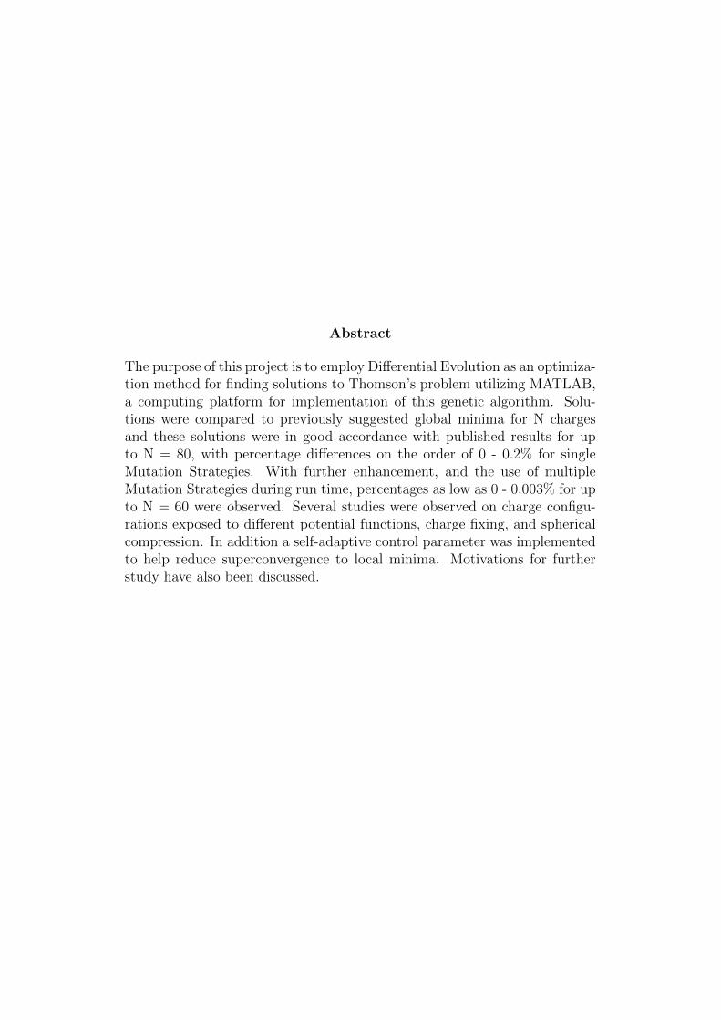
Abstract

The purpose of this project is to employ Differential Evolution as an optimiza-tion method for finding solutions to Thomson’s problem utilizing MATLAB,a computing platform for implementation of this genetic algorithm. Solu-tions were compared to previously suggested global minima for N chargesand these solutions were in good accordance with published results for upto N = 80, with percentage differences on the order of 0 - 0.2% for singleMutation Strategies. With further enhancement, and the use of multipleMutation Strategies during run time, percentages as low as 0 - 0.003% for upto N = 60 were observed. Several studies were observed on charge configu-rations exposed to different potential functions, charge fixing, and sphericalcompression. In addition a self-adaptive control parameter was implementedto help reduce superconvergence to local minima. Motivations for furtherstudy have also been discussed.

Contents

1 Introduction 3

2 Optimization Methods 52.1 Random Walks . . . . . . . . . . . . . . . . . . . . . . . . . . 52.2 Steepest Descent Method . . . . . . . . . . . . . . . . . . . . . 82.3 Simulated Annealing . . . . . . . . . . . . . . . . . . . . . . . 82.4 Genetic Algorithms . . . . . . . . . . . . . . . . . . . . . . . . 9

3 Theory of the Differential Evolution algorithm 113.1 Initialization . . . . . . . . . . . . . . . . . . . . . . . . . . . . 113.2 Mutation Algorithm . . . . . . . . . . . . . . . . . . . . . . . 143.3 Crossover Algorithm . . . . . . . . . . . . . . . . . . . . . . . 183.4 Selection Algorithm . . . . . . . . . . . . . . . . . . . . . . . . 203.5 Control Parameters . . . . . . . . . . . . . . . . . . . . . . . . 22

3.5.1 Weighting Functions . . . . . . . . . . . . . . . . . . . 223.5.2 Self-Adaptive Weighting . . . . . . . . . . . . . . . . . 23

4 Results 244.1 Comparison with Previous Results . . . . . . . . . . . . . . . 254.2 Comparison of Strategies . . . . . . . . . . . . . . . . . . . . . 304.3 Study of Charge Configurations . . . . . . . . . . . . . . . . . 364.4 Self Adaptive Weighting versus Manual Weighting . . . . . . . 434.5 Effects of Program Parameters on Convergence and Run time 464.6 Study of Compressed Spheres . . . . . . . . . . . . . . . . . . 504.7 Non-Coloumbic potentials . . . . . . . . . . . . . . . . . . . . 53

4.7.1 Squared and Cubed potentials . . . . . . . . . . . . . . 534.7.2 Lennard-Jones Potential . . . . . . . . . . . . . . . . . 55

4.8 Limitations and Further Error Analysis . . . . . . . . . . . . . 58

5 Conclusions 59

1

6 References 60

7 Appendix A 62

8 Appendix B 73

2

Chapter 1

Introduction

This project addresses the problem of finding the optimum, that is, theminimum energy configuration of N equal charges confined to the surface ofa sphere. The problem was first proposed by J.J. Thomson in 1904 [1] inrelation to his plum pudding model of the atom. The problem is of generalinterest not only to physicists but also to mathematicians, chemists andbiologists. The original problem, as defined by Thomson, concerns electronsinteracting through the Coulomb potential, however the scope of the problemhas been expanded to include power law potentials of the form;

U(r) =1

rn

Where n = 1 reduces to the Coulomb potential. Letting r1, r2, ... rNdefine the set of distinct position vectors confined to the unit sphere, thepotential function can now be described in the form;

U(r) =N∑

i,j=1,j>1

1

| ri − rj |(1.1)

With i and j both equal to integers; ri = [xi, yi, zi] and rj = [xj, yj, zj].There already exists a large literature on the Thomson problem. Early

work on the problem is described by Cohn [2]. A more recent survey isprovided by E. B. Saff and A. B. J. Kuijlaars, [3] with emphasis on the casewhere N is large. The Cambridge Cluster Database [4] provides a list ofexperimentally determined candidate solutions for n = 10 to 972 based onthe work of Wales and Ulker [5]

While numerous attempts have been made to find a general solution tothis problem, only special solutions have been found for cases where N is low.In many instances polyhedra have been used as geometric tools for describing

3

configurations, since the arrangement of points on a sphere can be visuallyrepresented by equivalent vertices of relevant polyhedra.[6]

Foppl found in 1912 solutions to a similar problem for up to N = 8 and10, 12 and 14 using spherical point systems but acknowledged that the N =4 case would fit a tetrahedron.[6][7] Later Fejes introduced another problem,essentially a variation of the Thomson problem where he sought to maximizethe minimum distance between N points on sphere.[8] This problem can bedescribed as a sphere packing problem, which seeks the largest diameterof N equal circles so that when placed on a sphere they do not overlap.Fejes proved an inequality which states there always exists two points witha distance less than or equal to;

d ≤

√4− csc2[ piN

6(N − 2)] (1.2)

Where d is the distance and for N = 3, 4, 6 and 12 eq(1.2) the inequalityholds. This inequality was also used to find N = 8 and N = 20 by H.Rutishauser. [8] Similar again to Fejes problem is Tammes problem whichis also a sphere packing problem only applied to pollen grains with poreconfigurations. [9] One of the main reasons why no general solution has beenfound is that configurations don’t rely solely on the symmetries of the sphere.As a result optimization techniques have been employed in order to find moreaccurate solutions [6][7][10][11].

Even though Thomson’s model of the atom has long been replaced byexperimentally more accurate models, the applications of his model haveproven useful in other scientific fields such as biology and chemistry. Com-putational methods can be extended with a modified Thomson problem tofinding atomic configurations for molecules, where atom locations correspondto the vertices of polyhedral structures in spherical molecules or likewisespherical viruses where capsid locations would correspond to the verticesinstead, for instance buckminsterfullerene or C60 would form a truncatedicosahedron if some strain element was included for the hybridisation of car-bon orbitals.[12][13][14] The problem can be further modified to show howpoint charges should arrange themselves under compression of the sphere toa disk (which will be shown in a later chapter) or even for elongated spheres.

This report investigates the solutions obtained via a Genetic algorithm,specifically Differential Evolution as outlined by Storn and Price [15] anda self adaptive Differential Evolution algorithm, the latter of which is aseemingly unreported method for finding solutions to the Thomson Prob-lem.[16][17]

4

Chapter 2

Optimization Methods

Many optimization techniques have previously been employed on the Thom-son problem. Weinrach et al used a Random Walks method on the Thomsonproblem in 1990.[18] A. M. Livshits and Yu. E. Lozovik previously used aSteepest Descent method. [19] S.C Kirkpatrick et al used Simulated Anneal-ing on the Thomson problem. [20] In 1975 John Holland outlined the basis forGenetic Algorithms which have subsequently been employed on the Thom-son problem. [21] In the following sections several optimisation techniques,previously applied to the Thomson problem, are briefly described.

2.1 Random Walks

Numerous optimisation methods were applied to Thomson’s problem duringthe second half of the 20th century, a simple technique is the random walksmethod as outlined by Weinrach et al. [18] When using this method for theThomson problem the objective function, (which will be generally referred toas the potential function in this paper), is sampled by randomly generatedposition vectors or points on the surface of a sphere, using a Monte Carlo(MC) method. MC methods are algorithms which use random numbers tosolve problems which are either deterministic or probabilistic in nature. Amajor limitation of the Random Walks method is that it has a ”greedy”selection criterion, in other words a ’trial’ vector with a lower objective func-tion is always accepted over the base vector, which is the vector that wasthe trial vector for the previous iteration. If the magnitude of a trial vectorconfined to a local minimum is too small then the trial vector will never havean objective function larger than the base vector, which in turn confines thesolution to that local minimum. Additionally this algorithm may be inhib-ited by its starting point; for instance in a case where the objective function

5

is multi-modal, the algorithm may converge to a local minimum as opposedto a global minimum, due to a local minima being sampled by the trial vectorfirst (see Figure 2.1)

Figure 2.1: Demonstrating with a non-specific objective function the localand global minima of the peaks function from MATLAB

6

Additionally a simple way of visualising the vectorization of this problemwould be to create a contour plane where the coloured contours define theoptimal fitness of the objective function. Here the position vectors randomlysample the objective plane (see figure 2.2)

Figure 2.2: Contour graph of Random Walks method. Red and yellow con-tour lines indicate regions of lower potential, while blue lines indicate regionsof higher potential. Vectors sample the contour plane randomly.

7

2.2 Steepest Descent Method

A. M. Livshits and Yu. E. Lozovik used a modified derivative based SteepestDescent method of iterating for finding solutions to Thomson’s problem. [19]The Steepest Descent method uses the gradient of the objective function tofind the nearest local minimum. In this example, once a pre-determinedconvergence criterion has been met, the program checks the stability of theconfiguration by generating a large amount of random movements, if theenergy continues to decrease the program starts again. T.Erber and G.MHockney [22] also used a steepest decent method for the Thomson problem.They noted that the number of metastable configurations grows exponentiallywith an increase in number of charges N and that the basin or catchmentregion for the global minimum is often small compared to those of otherminima.[22][23][24] This essentially leads not only to greater computing timesbut a greater chance of convergence to local minima.

2.3 Simulated Annealing

Simulated annealing (SA) gained its name from the concept of annealing,which is the process of cooling a molten substance in order to grow a crys-talline structure.[20] Global optimization methods such as SA enhance theprobability of points not being inadvertently confined to a local minima, mak-ing such methods more preferable to the previously mentioned multi-modalmethods. The SA algorithm retains all deviations in position which decreasethe potential of the system while allowing for some less optimal deviations.The probability of accepting less optimal configurations decreases with ev-ery evaluation. The Metropolis algorithm[25] is used to select which randomincrease in deviation should be accepted and is given by the equation;

θ = e−dβT

The algorithm looks and behaves similarly to the Boltzmann equation, thetemperature T decreases over a number of iterations and simulates the cool-ing of the system, d is the energy difference between the less optimal potentialand the current potential and β is a control factor. The analogy of annealingcan be extended; if the molten substance was cooled too fast the crystallinestructure would become disordered resulting in a local minimum, while cool-ing slowly would result in the true crystalline ground state being obtained,which is equivalent to the global minimum being found.[15]

8

2.4 Genetic Algorithms

Genetic algorithms, which are an offshoot of evolutionary algorithms, areglobal search algorithms or heuristics which can be used as optimizationmethods on problems such as the one suggested by Thomson. [15][21] Mostgenetic algorithms contain similar mechanisms to natural selection and genetheory and utilize biological concepts such as mutation, crossover, survival ofthe fittest, inheritance etc. in order to evolve towards better solutions. Thealgorithm typically starts with a population initialization of which randomlygenerated trial members or individuals are created. Each member makes upa population and for every generation the individual members are evaluatedusing an objective function to determine the fitness of each member. Ge-netic operators are then implemented in order to create future generationsby modifying members of the current population. (Mutation, Recombina-tion etc.). Modified members that have a higher fitness than members of thecurrent generation survive to the next generation (Selection). Populationscontinue evolve towards better solutions for the function to determine thefitness of each member and ultimately will converge on the best, or global,solution. Population sizes vary depending on the size and scope of the prob-lem. Sometimes ’seeding’ is used which places population members close towhere optimal solutions are predicted to exist. Each population is composedof trial solutions represented as strings or arrays of bits leading to a Binary orGray coding implementation to help better convergence. Genetic algorithmsare not entirely dependent on the use of bit strings and for variables in con-tinuous search spaces a real number representation is more instinctive. [26]Such a representation was first proposed by Storn and Price in their Differ-ential Evolution (DE) algorithm. [15] For the Thomson problem, DifferentialEvolution (DE) overcomes the need to program using binary numbers since itdeals with vectorization of real numbers. DE is a global optimization meta-heuristic which uses the same concepts as other genetic algorithms, mainlymutation, crossover and selection, all of which will be discussed in later sec-tions, to arrive at better solutions to an optimization problem.

9

A general schematic of how the various genetic operations are imple-mented in DE are described in figure 2.3.

Figure 2.3: Schematic of DE algorithm, at each stage the objective functionis evaluated for different sets of solution vectors.

This schematic will be referred to again when the genetic operations areexplained in detail in later sections.

Closely related to genetic algorithms and evolution strategies is Parti-cle Swarm Optimization (PSO) [27], which was developed for the Thomsonproblem by Andrei and Elena Bauta. This model is analogous to and basedon the social behaviour of bird flocking.

10

Chapter 3

Theory of the DifferentialEvolution algorithm

Differential evolution is used to find solutions to non-differential, nonlinearand multimodal functions. Randomly initialized vectors are created to makeup a population of potential solutions, which in turn ’evolve’ to find bet-ter solutions. For each iteration, referred to formally as generations in thispaper, new vectors are created by combining vectors from the current popu-lation in a process called Mutation. These new vectors are then mixed to apredetermined ’target’ vector in a process called Crossover. If the ’trial’ vec-tor created by these processes has a lower objective solution than previously,the ’trial’ vector is retained into the next generation in a process known asSelection. [28]

3.1 Initialization

In order to minimize computing time, the Cartesian coordinates are changedto spherical coordinates, which essentially means the potential function isdefined by two coordinates rather than three (The charges are coincided tobe confined to a unit sphere so, radius = 1 ). The variables are given as theangles theta and phi, where theta is the inclination angle with a range [0,π]and phi is the azimuthal angle measured in the equatorial plane with range[0,2π], then;

11

x = cosθsinφ

y = sinφsinθ

z = cosφ (3.1)

The potential function from eq(1.1) can be expressed in terms of x, y and zas;

U(x, y, z) =∑ 1√

(xi − xj)2 + (yi − yj)2 + (zi − zj)2

=∑ 1√

2− 2(xixj + yiyj + zizj)(3.2)

(Since r2 = x2 + y2 + z2 = 1). Substituting in eq(3.1) for x, y and z;

xixj = cosθicosθjsinφisinφj

yiyj = sinφisinφjsinθisinθj

zizj = cosφicosφj (3.3)

Using the trigonometric identity cos(A − B) = cosAcosB + sinAsinBwhere A = θi and B = θj

U(φ, θ) =∑ 1√

2− 2(cosφicosφj + sinφisinφjcos(θi − θj))(3.4)

This now gives the potential as a function of phi and theta. Before theDifferential Evolution algorithm begins, the first generation of charge config-urations is created. An array containing relevant information on the popula-tion of spheres is created, xi,D,N , where every sphere is given an index i whichrange from 1 to P, the total population number. Each sphere is appointedN point charges. The first charge on each sphere in the population, is heldat a fixed position while the positions of the remaining N-1 charges on eachsphere are randomly generated. The index D is either 1 or 2 and representsthe theta and phi coordinates of each charge respectively. The purpose of thefixed charge is to reference the position of other charges relative to the posi-tion of the fixed charge for all spheres or in other words each sphere has an

12

invariant point and allows for consistency when analysing charge positionson all spheres. The positions of the second (n = 2) charge up to the lastcharge (n = N) are created using a random number generator, which outputsa value from zero to one, multiplied by the upper bounds of the angle inquestion. However, due to the surface area of the sphere being proportionalto sinφdθdφ random points placed on the sphere will be concentrated nearthe poles. A correction is made in order to ensure that the charges are dis-tributed uniformly on the sphere. The initial population of charges is definedby;

xi,1,n = cos−1(2Randi,[0→1] − 1), i = 1, 2, 3..., P n = 2, 3, 4..., N.

xi,2,n = 2πRandi,[0→1], i = 1, 2, 3..., P n = 2, 3, 4..., N.

For n = 1 the fixed positions are xi,1,1 = π2

and xi,2,1 = 0, i.e. a point on theequator of the sphere.

The potential energy of each sphere in the population is then evaluatedfrom the potential function. It is important to note that for every subsequentgeneration the corresponding potential energy is evaluated for the chargedistribution on each sphere however the DE algorithm is used to determinethe charge distribution in subsequent generations.

13

3.2 Mutation Algorithm

From the second generation (i.e. the second iteration of the algorithm) on-ward the population of spheres is subjected to the DE algorithm. Mutationmixes the parameters of our position vectors from one generation to the nextby finding a weighted difference of the position vectors of two randomly se-lected charges and adding the resultant position vector to a third randomlychosen ’base’ vector creating a Mutation or ’trial’ vector (see figure 3.1).There are various types of Mutation strategies as outlined by Storn andPrice [15]. For the DE algorithm used in this work the following mutationstrategies were tested;

Strategy 1: - DE/rand/1Strategy 2: - DE/local − to− best/1Strategy 3: - DE/best/1withjitterStrategy 4: - DE/rand/1withper − vector − dither

The first strategy is known as DE/rand/1. Here three target vectorsXi,G from the current population are selected by randomly chosen indicesA,B and C and where A, B and C are all different indices, i.e. no two valuesare equal. XA,G is the base vector and XB,G and XC,G are called DifferentialVectors. The Mutation vector Vi,G, is calculated from;

Vi,G = XA,G + F (XB,G −XC,G) (3.5)

where F is a weighting function that controls the size of the resultantdifference vector, (XB,G −XC,G).

Strategies 4 is essentially a modified version of Strategy 1, given by;

Vi,G = XA,G + ((1− F )rand[0→1] + F )(XB,G −XC,G) (3.6)

For Strategy 2 additional differential vectors for the current best Xbest,G andcurrent member Xi,G are included such that;

Vi,G = XA,G + F (XB,G −XC,G) + F (Xbest,G −Xi,G) (3.7)

For strategy 3 the ’base’ vector is the current best vector Xbest,G.The size of any population has a lower limit of 4 or 5 depending on the

strategy outlined since the randomly chosen indices must be different.

14

The following diagram can be used to visualise the formation of the Mu-tation vector from eq(3.5);

Figure 3.1: Contour plot showing the Mutation operation using scheme 1.

15

The Pseudocode for strategies 1 and 3 are as follows;

Strategy 1:

%FM_pop are Trail_pop are arrays

%which contains coordinates for each charge

%F is the weighting

FOR each population member i

WHILE neither A or B or C are equal

pick random FM_pop[i,A];

pick random FM_pop[i,B];

pick random FM_pop[i,C];

END WHILE

FOR each charge k

IF calulation is within bounds(0-pi) or (0-2*pi) THEN

Trail_pop[i,k] = FM_pop[C,k] - F*(FM_pop[A,k] - FM_pop[B,k]);

ELSE

%set above equation in bounds

...

Trail_pop[i,k] = FM_pop[C,k] - F*(FM_pop[A,k] - FM_pop[B,k]);

ENDIF

END LOOP

END LOOP

RETURN Trail_pop

16

Strategy 3:

%FM_pop,Trail_pop and best_pop are arrays

%which contains coordinates for each charge

%F is the weighting

FOR each population member i

WHILE A and B are not equal

pick random FM_pop[i,A];

pick random FM_pop[i,B];

END WHILE

FOR each charge k

IF calulation is within bounds(0-pi) or (0-2*pi) THEN

Trail_pop[i,k] = best_pop[i,k] - F*(FM_pop[A,k] - FM_pop[B,k])

ELSE

%set above equation in bounds

...

Trail_pop[i,k] = best_pop[i,k] - F*(FM_pop[A,k] - FM_pop[B,k])

ENDIF

END LOOP

END LOOP

RETURN Trail_pop

Note: Equations need to be set within the bounds of [0 - π] for θ and [0 -2π] for φ in order to create 2D graphs for charge positions.

17

3.3 Crossover Algorithm

A random number generator is used to determine if the Crossover Algorithmwill be implemented given a pre-defined probability of occurrence and forthat reason the population of ’trial’ vectors from section 2.2 may or maynot be passed directly to the Selection Algorithm. The Crossover Algorithmoperates in an analogous manner to the way a child inherits its genes fromits parents. The Crossover Algorithm is applied directly after the mutantvectors are created and utilizes binary masking to form a trial vector. Twoopposing matrices are created with opposing random values of 1 or 0 and aredefined as Mp and Mu. For example, for 5 charges the matrices could takethe form;

Mp =

1 10 11 11 00 0

Mu =

0 01 00 00 11 1

(3.8)

Where the trial vector is defined by;

Vi,G+1 = Xi,G ◦Mp + Vi,G ◦Mu (3.9)

The ◦ operator here denotes the Hadamard product which simply multi-plies the individual elements of one matrix with the corresponding elementsof another matrix to create a new matrix. For example with three charges;

Vi,G+1 =

xθ,1 xφ,1xθ,2 xφ,2xθ,3 xφ,3

◦1 0

0 11 1

+

vθ,1 vφ,1vθ,2 vφ,2vθ,3 vφ,3

◦0 1

1 00 0

(3.10)

=

xθ,1 00 xφ,2xθ,3 xφ,3

+

0 vφ,1vθ,2 00 0

(3.11)

=

xθ,1 vφ,1vθ,2 xφ,2xθ,3 xφ,3

(3.12)

The new matrix as seen in eq(3.12) now contains elements from both Xi,G

and Vi,G. The Crossover Algorithm is controlled by a probability CR which

18

was empirically determined at 0.7 for this project.

Ui,G+1 =

{Vi,G+1 if rand[0→1] ≤ CRXi,G else

(3.13)

Ui,G+1 is the set of vectors which will be passed to the potential function.Figure 3.2 graphically represents the Crossover operation.

Figure 3.2: Crossover occurring between two spheres.

19

3.4 Selection Algorithm

The Selection Algorithm decides whether the ’trial’ vector or the current vec-tor should be retained into the next generation. If the trial vector is chosenthan it replaces the current vector. Two algorithms for choosing the coordi-nates of the charges on each sphere in subsequent populations were used inthis project: 1) Greedy Tournament, where each member of the populationof spheres competes against the correspondingly indexed population mem-ber of the new population, as given by eq(3.14) and demonstrated in thediagram shown in figure 3.3; 2) The current population of spheres is sortedaccording to the potential energy of each sphere, with the sphere having thelowest energy configuration being ranked highest. Only a pre-defined ’best’percentage survives to the next generation while the remainder of the pop-ulation consists of new population members regardless of whether they arefitter or not. A sorting algorithm is used to rank the spheres from lowestto highest potential, lowest being the more optimal potentials. The basic’greedy’ Selection Algorithm (algorithm always picks the optimal solution),is defined as;

Xi,G+1 =

{Ui,G+1 if f(Ui,G+1) < f(Xi,G)Xi,G else

(3.14)

The population is then re-indexed depending on the potential for eachsphere. A program has been written to implement both of these methods(or a mixture of both) though the primary method used is the first methodas sorting populations can be costly and no general advantage was observedover using either method.

20

Figure 3.3: Schematic of DE algorithm.[15] (vectors are capitalized in thispaper, but have the same physical purpose ). This flow-chart is a moredetailed version of the previously described schematic in section 2.4 (Seefigure 2.3).

21

3.5 Control Parameters

3.5.1 Weighting Functions

The two main control parameters within the DE algorithm are the crossoverprobability CR and weighting function F, as described above. The Crossoverprobability remains constant as previously stated however the weighting func-tion is altered depending on the strategy employed and instead of being con-stant may linearly/exponentially increase or decrease from one generation tothe next. A major problem is to try and empirically evaluate the best valueor strategy for the varying weighting function since every strategy has a dif-ferent convergence criteria i.e. one strategy may be ’greedy’ and try to find asolution in few generations while another may be slow and take many gener-ations. Therefore a self-adaptive method for controlling the weight functionfor DE was introduced [16][17]. A list of the weighting functions used andtested is as follows.

Linearly increasing:

F = aGi

Gmax

(3.15)

Linearly decreasing:

F = a(1− Gi

Gmax

) (3.16)

Exponential:

F = a(exp[Gi

Gmax

]) (3.17)

Negative exponential:

F = a(1− exp[ Gi

Gmax

]) (3.18)

where a is a constant that was empirically evaluated as 0.3, Gi is the gener-ation index and Gmax is the last generation index (0.3 is the default weightif none of the above equations are selected).

22

3.5.2 Self-Adaptive Weighting

The Self Adaptive control parameter for the weighting as outlined by J. Brestet. al is determined as follows; [16]

Fi,G+1 =

{Fl + rand1Fu if rand2 < T1Fi,G else

(3.19)

Fl and Fu remain constant with values of 0.1 and 0.9 respectively and as aresult the weighting function will produce values between [ 0.1 → 1.0]. T1has a value of 0.1, and so this randomized weighting has a 10% chance ofbeing implemented.

In order to make the randomized weighting and current weighting com-petitive two scenarios must be created. The first senario consists of a pop-ulation of trial vectors being created using the current weighting functionand the trail vectors being evaluated with the potential function. The sec-ond scenario is similar but instead the trial vectors are created using therandomized weighting as determined in eq(3.19). The scenario which is thenmore optimal defines whether the weighting function should change.

23

Chapter 4

ResultsA brief summary of the experiments performed in this project are as follows;

• The Thomson problem for N charges on a sphere (where N = 2 →100) is compared with the best known solutions obtained by previousoptimization techniques (see section 4.1),• The different strategies (outlined in section 3.1) are studied in order to

determine the best strategy for the Thomson problem (see section 4.2).

• A study on charge configurations is undertaken to investigate the rel-evance of fixed charges, in other words charges which are invariant togenetic operations, on the formation of charge positions on the surfacesphere (see section 4.3),• A comparative study is made between the Self-Adaptive weight control

parameter and adaptive/non-adaptive weight control parameter (seesection 4.4),• The effects of program parameters on convergence and run-time are

studied (see section 4.5),• The Thomson problem is extended to an ellipsoidal shape (see section

4.6), other potentials are studied (see section 4.7),• Finally the limitations of DE and other error analysis is discussed (see

section 4.8).

The specifications of the laptop used in these experiments are given in Table4.1. MATLAB 7.1 was the programming platform used in this project andis ideal for numerical calculations that use vectors.

System Intel(R) Core(TM) i5-2430M CPU @ 2.40GHz, 2401Mhz,Processor 2 core(s) 4 logical processorsRAM 5.95GB (installed) 4.21GB (available)

Table 4.1: table showing laptop specs.

24

4.1 Comparison with Previous Results

Known solutions for the global minima for the Thomson problem, where N ≥10, were taken from The Cambridge Cluster Database [4]. The results are thework of David J. Wales and Sidika Ulker [5] and are given to seven decimalplaces. For 2 ≤ N < 10 results were taken from ”Energy Minimization ofPoint Charges on a Sphere with Particle Swarms” by Andrei Bautu and ElenaBautu [27]. Two Strategies were used to obtain the following results; Strategy1 with Self-adaptive weighting for 2 ≤ N ≤ 10 and population maximum of400, Strategy 3 for N>10 for population maximum of 700. The followingtable outlines the results obtained. (Table 4.2)

N Prev. Potential Standard Percentage time Gen.Measured Measured deviation difference taken Max.potential using DE (%) (s)

2 0.5000000 0.5000000 0 0 4 1003 1.7320508 1.7320508 0 0 15 3004 3.6742346 3.6742346 0 0 24 4005 6.4746915 6.4746915 0 0 46 6006 9.9852814 9.9852814 0 0 71 8007 14.4529774 14.4529774 0 0 113 10008 19.6752879 19.6752879 0 0 117 10009 25.7599866 25.7599865 0 4x10−7 126 100010 32.7169495 32.7169494 0 3x10−7 156 120015 80.6702441 80.6723749 2.86x10−5 2.6414x10−3 432 150020 150.8815683 150.9087020 2.641x10−4 0.0179834 935 250040 660.6752788 661.5827689 9.7709x10−3 0.1373580 5693 600060 1543.8304010 1545.5745970 1.73153x10−2 0.1777524 19060 1000080 2805.3558759 2809.0886473 4.61007x10−2 0.1330587 48101 15000

Table 4.2: Table shows previously obtained potentials with results gatheredfor this project. Generation maxima range from 100 to 15000 with a longestrun-time of approximately 13.4hrs. Potential energy values are accurate to ±1x10−7. The Standard deviation was determined from the last 10 generationsof each run.

25

Long run-times are needed in order to maintain a certain degree of accu-racy, for instance when N = 40, 60 and 80 incremental changes in generationmaximum are on the order of 4000 to 5000 to maintain a percentage accuracyof ∼ 0.1% - 0.2%.

Results can be improved by switching between strategies during run-time, which was done for N = 60 with a generation maximum as low as4000, improving the percentage difference between the known value and ex-perimentally found value to ∼0.003%. However, it is difficult to empiricallyevaluate at what point in the run time and for what convergence criterionthese switches should occur, especially since they change for different val-ues of N, and so switching strategies are omitted from the general results.One method to overcome this problem, by self adaptation, was attempted,as outlined in section 4.4 (Strategies 1 and 3 were used for switching).

Figure 4.1 shows the charge configuration for N = 60 from Table 4.2 as aprojection of the surface of the sphere onto a 2D plane. Visually it is possibleto see a high level of order associated with this configuration, however somedefects are present.

Figure 4.1: 2D Charge configuration for N = 60, From results given in Table4.2.

26

Figure 4.2 shows little or no defects and is ordered. A general wavepattern can also be seen, essentially showing a highly ordered charge config-uration.

Figure 4.2: 2D Charge configuration for N = 60, for Strategy switch givinga potential energy of 1543.8757727.

Most charge configurations have a high degree of triangulation betweenpoints (i.e. points that form triangulated patterns on 3D sphere), which istypically how charges configure for the Thomson problem, though in figure4.1 a pentagonal shape is observed at θ = 1.5 and φ = 5. A large standard de-viation in the potential energy was observed for the last 10 generations whichsuggests that the configuration had not yet converged to a local or globalminimum (For more detail see section 4.3). These images were rendered inPOV-Ray.[29] No deviation was observed for the charge configuration givenin Figure 4.2. 3D images for N = 20, 40, 60 and 80 are shown in the belowfigures 4.3 - 4.6. Despite N = 40, 60 and 80 being most likely local minimaa high level of order is still observed.

27

Figure 4.3: Charge configuration for N = 20.

Figure 4.4: Charge configuration for N = 40.

28

Figure 4.5: Charge configuration for N = 60.

Figure 4.6: Charge configuration for N = 80.

29

4.2 Comparison of Strategies

Table 4.3 shows the performance of each strategy for a pre-determined num-ber of generations. The initial population of spheres for each strategy isthe same for a given charge number N. The weighting function in this casefollows a negative exponential curve versus generation number eq(3.18). Apopulation maximum of 400 was used.

N potential Strategy 1 Strategy 2 Strategy 3 Strategy 4

5 6.4746915 6.5012242 6.6672681 6.4746915 6.560748410 32.7169494 32.9923685 32.7368405 32.8620634 34.344472215 80.6702441 81.3171397 83.4536538 80.7632577 85.682503620 150.8815683 152.1675597 159.2065737 151.2418280 157.804105030 359.6039459 363.0592448 377.8094840 360.5360655 380.476975060 1543.8304010 1566.1146148 1636.6584255 1548.0360076 1627.3732321

Table 4.3: Table showing potentials for different strategies as compared toknown best (Gen Max = 100, 500 ,1000, 1500, 3000 and 6000 for N = 5, 10,15, 20, 30 and 60 respectively).

The choice of using a negative exponential weighting as opposed to usingother weightings was implemented for two reasons - first it approximates aconstant weighting value for a large portion of the run while towards theend of the run allows for small differences in the mutation vector, or in asense one assumes the value is converging to the global minimum so smallervariance in the position vectors is more desirable. Figures 4.7 to 4.10 showthe convergence of the best (Indicated by the blue line) and worst populationmember (indicated by the red line) for each strategy where N = 15. Graphshave been scaled logarithmically in order to see separation between best andworst members. Population reinitialization accounts for variations in worstvalue which will be discussed later.

30

Strategy 1

Figure 4.7: Potential energy as a function of generation number for Strategy1 implemented with N = 15 charges.

Strategy 2

Figure 4.8: Potential energy as a function of generation number for Strategy2 implemented with N = 15 charges.

31

Strategy 3

Figure 4.9: Potential energy as a function of generation number for Strategy3 implemented with N = 15 charges.

Strategy 4

Figure 4.10: Potential energy as a function of generation number for Strategy4 implemented with N = 15 charges.

32

Strategies 1 and 3 were the best for the majority of the runs. Strategy3 converges the fastest of all strategies and always has very little deviationbetween the worst and best member of the population of spheres. Strategies2 and 4 performed the worse than Strategies 1 and 3. A large difference inpotentials was observed between worst and best member for both strategies atthe end of run time suggesting it would take much larger run times before thepopulation would converge. For this reason strategy 1 and 3 were employedmost often for experiments as they are more cost effective for run time.Increasing the generation maximum for each run also increases the accuracyof results.

It is important, however, to realise that for different weightings the re-sults would vary as some weighting functions are more suitable for specificstrategies. For example taking the case of 15 charges with a linear decreasingweighting eq(3.16) (Table 4.4);

N potential Strategy 1 Strategy 2 Strategy 3 Strategy 4

5 80.6702441 80.7646659 81.3952184 80.8267639 82.4866463

Table 4.4: Table showing potentials for different strategies for N = 15

A marked improvement for the potential for Strategies 1,2 and 4 is ob-served while strategy 3 has a higher potential. Strategy 1 is only marginallyless optimal than strategy 3 for the negative exponential weighting. The lin-early increasing weighting eq(3.15) and the exponentially increasing weight-ing eq(3.17) were also tested. Results were less optimal than both decreasingweightings. This was to be expected since after a certain number of gen-erations the differential vector may become too large to sample the globalminimum for Strategy 1 and too small for initial generations for Strategy3. Figure 4.11 shows Strategy 1 with a linearly increasing weighting for 15charges. Figure 4.12 shows Strategy 3 for an increasing exponential weight-ing.

33

Strategy 1

Figure 4.11: Potential energy as a function of generation number for Strategy1 for N = 15 with logarithmic scaling, potential is 81.0142541 with standarddeviation of 0.

34

Strategy 3

Figure 4.12: Potential energy as a function of generation number for Strategy3 for N = 15 with logarithmic scaling, potential is 81.0220352 with standarddeviation of 0.0159543.

35

4.3 Study of Charge Configurations

For this experiment the DE algorithm is run with the same number of chargeson different spheres. The program makes five runs for a given value of Nand the resulting coordinates and statistics are saved and then compared.To start, 400 spheres per generation, with 2000 generations are used. Thesimulations are run with seven charges with one of the charges fixed. Figure4.13 shows the charge configurations for all five runs as a function of φ andθ are shown. Here the coordinates change for some runs and remain thesame for others. This is a result of there being multiple orientations forconfigurations that give the same minimum energy, for example if there were3 charges, the configuration could be confined to any great circle to intersectthe sphere, not solely the equator.

Figure 4.13: Charge configuration for N = 7, with one fixed point.

This in a sense makes it more difficult to interpret if a configuration hasconverged to the right value, although in the above graph one can see alevel of symmetry arising around phi equal to pi and theta equal to pi/2 forthe orange, red and black markers suggesting there is a high level of orderto these configurations. Statistically (potential, error... etc.) these chargeconfigurations give similar results.

36

With two charges fixed at each pole as seen in figure 4.14 there is adegree of freedom around the equator and hence the final coordinates aredifferent for each sphere, however it is important to note all 5 charges arespaced equally for each sphere, so essentially all the spheres have the sameconfiguration as each coordinates would map onto each other under a simplerotation.

Figure 4.14: Charge configuration for N = 7, with two polar fixed points.

In fact for any sphere where 2 charges are fixed at each pole and given thatsphere gives a true configuration, it should be possible to map configurationsunder rotation (see figure 4.14) unless the configuration has chirality.

37

Figure 4.15 shows the effect on the charge arrangements for two fixedcharges, one polar and one equatorial. All five spheres have the same coordi-nates which is to be expected since the degree of freedom for the remainingcharges are restricted; the configuration for N = 7 consists of 5 charges mak-ing a pentagonal shape around the equator with two charges on each pole .For all three cases Figure 4.13 to 4.15 the statistics were equal showing negli-gible or no deviation caused by fixing charges; Potential equal to 14.4529774,Standard Deviation equal to 0.0000000 and a percentage difference betweenthe calculated results and the known global minimum of 0.0000000%.

Figure 4.15: Charge configuration for N =7, with two fixed points, one polarand one equatorial.

38

Another aspect which can be discussed under the investigation of chargeconfigurations is the concept of how to define highly ordered local minima.For example, figure 4.16 and table 4.5 the configuration denoted by the orangecircle has the highest percentage deviance from the global minimum and whileit is very ordered, it has a different configuration than the other 4 results.

Figure 4.16: Figure showing two polar fixed points for N = 17 with a popu-lation number of 400 and Gen. Num. of 4000

Colour Potential Standard Deviation Percentage error

Black 106.0517748 0.0000070 0.0013Orange 106.1507641 0.0003760 0.0946Blue 106.0518891 0.0000047 0.0014Green 106.0741286 0.0000754 0.0223Red 106.0571122 0.0000497 0.0063

Table 4.5: Statistics for 5 different charge configurations.

39

The other four charge configurations converge to the real global minimumand the orange marked configuration appears to be converging to a localminimum configuration. What is of great interest though is the fact thatthe next nearest configuration to the local minima (green marker) has apercentage difference on the same order of magnitude, meaning that boththe local and global minimum would have very similar potentials, which isunusual for a low value of N. Furthermore the standard deviation is oneorder of magnitude higher for the orange and with further investigation ofthe convergence graph in figure 4.17, one can determine that the orangeconfiguration is not in fact metastable and therefore cannot be consideredconverging to a local minimum.

Figure 4.17: Convergence graph of N = 17 corresponding to orange markedconfiguration. Note that the best and worst values are still decreasing at thelast generation.

Therefore standard deviation can be used not just to merit the accuracyof the results but also as a tool in defining whether a solution has convergedor not.

40

Not all configurations will have charges at each pole (or two points di-rectly opposing each other on the surface of sphere). For example when N =9 (Pop. Num. = 400 and Gen. Max. = 4000), one charge is fixed and theconfigurations are shown in figure 4.18. Here only two of the runs gave thesame configuration, however the error and standard deviation were equal foreach run ( Potential = 25.7599865, Standard Deviation = 0.0000000, percent-age difference between Global min = 0% ) leading to the same conclusionsas in the previously discussed case N = 7. While visually difficult to see, theformation takes an approximate 1-5-3 formation (3 points on a plane and 5points roughly on a plane which would intersect the sphere plus an additionalpoint) or an exact 3-3-3 formation (allowing for depth in 3D graph). Howeverif we were to fix two points at each pole the formation changes to a different3-3-3 formation (the central point hides the polar opposite); figure 4.19. Inmore detail for one fixed point 3 points would intersect a great circle andhave a distance of 2

3π distance between them however for two fixed points 3

points intersect a great circle with two points exactly opposite to each otherand another point at a fixed distance of 1

2π between the two polar points.

In essence by forcing the configuration to have two fixed points a new globalminimum is created for N=9 and this potential is higher than it would befor one fixed point.

41

Figure 4.18: 2D charge configuration for N = 9 with one fixed charge (left)and 3D charge configuration for N = 9 (right).

Figure 4.19: 2D charge configuration for N = 9 with two fixed charges (left)and 3D charge configuration for N = 9 (right).

42

4.4 Self Adaptive Weighting versus Manual

Weighting

A great advantage that self-adaptive control parameters have over manualcontrol parameters is the ability to interchange between strategies withoutneeding to experimentally determine the best weighting for each strategy.This also reduces the number of initial parameters to just the strategies,generation maximum and population maximum. A marked improvement forminimum energy was observed over lower values of N for the self-adaptiveweighting however at N ∼ 15 a decrease in accuracy was observed (see Table4.6 in section 4.5 for confirmation)). As a result 15 charges were chosen asa basis for observing switching between Strategies with self-adaptive weight-ing. Three scenarios were tested; Strategy 1, Strategy 3 and Strategy 3 witha switch to Strategy 1 for a predefined generation index. Figures 4.20 and4.21 show the convergence graphs for Strategy 1 and 3 respectively. The po-tentials were 80.7045893 for Strategy 1 and 80.8150423 for Strategy 3 (Withpercentage difference between previously obtained potential value of 0.043%and 0.179% respectively). Only a small level of population re-introductionwas used for these results, since strategies would have a biased improvement(see section 4.5 for more detail) leading to results that are more difficult tointerpret. The same initial population was used for all three test runs witha generation maximum of 1500. The percentage difference for Strategy 1(4.3x10−2%) is an order of magnitude higher than the percentage obtainedin section 4.1 for Strategy 3 (2.6414x10−3%) showing that for higher valuesof N, Strategy 1 with self-adaptive weighting is still a less optimal methodthan Strategy 3 with negative exponential weighting.

43

Figure 4.20: Strategy 1 with Self Adaptive weighting.

Figure 4.21: Strategy 3 with Self Adaptive weighting. Best and worst mem-bers prematurely converge.

44

A test run was then carried out for both Strategies, with the first 10generations utilizing Strategy 3 and the remaining utilizing Strategy 1 (seefigure 4.21). A short generation run for Strategy 3 was chosen to insurethe population would still maintain a level of diversity (i.e. not convergetoo soon). Results found a marginally more optimal potential of 80.6998607with a percentage difference of 0.037% compared to the previously obtainedpotential. To draw more conclusive results, one could try more extensivepopulation re-introduction techniques in conjunction with multiple strategyswitching in order to find more optimal solutions as this is essentially how N= 60, with a percentage difference of ∼0.003%, was obtained in section 4.1.

Figure 4.22: Strategy 3 runs for first 10 Generations before switching toStrategy 1, Leading to a marginally better percentage difference (3.7x10−2)for Strategy 3 without Self-Adaptive weighting.

45

4.5 Effects of Program Parameters on Con-

vergence and Run time

Two major issues when dealing with optimization methods are how cost ef-fective (measure of robustness, speed etc.) the program is and how well doesit converge to the desired value. Of course these problems don’t rely solyon the competences of the programmer but more the nature of the problemitself. As mentioned previously Thomson’s problem has an exponential in-crease in the number of metastable states for higher N values leaving theproblem itself with an inherent difficulty for finding solutions. As a result asN increases so will the computing time. The other key issue, convergence,depends mainly on how diverse a population is. For instance in the case ofstrategy 3 where the mutant vectors always depend on the best vector of theprevious generation for high N values and after a certain number of genera-tions all the vectors will ultimately converge to the same value resulting inthe best and worst population member being equivalent. Once this happensthe mutation and crossover operations cease to find new vectors and the pop-ulation becomes static. One solution to stop a population becoming staticis to forcibly re-introduce new configurations with random position vectors(See figure 4.23).

Figure 4.23: Graph of best and worst values each population for N = 20,increases in the red fluctuating line indicates a population re-introduction.

46

Here, the best member or percentage of members is retained. The pop-ulation re-introduction occurs before Mutation and Crossover operations inorder to influence new populations. Only when the population is initiallydiverse will fluctuations in the worst member be observed, this however doesnot mean the population re-introduction has stopped working as this methoddoes not alter greatly the diversity of a population but rather stops it fromremaining static. The reason for this is simply down to the selectivity of thegenetic operations rejecting most of the random vectors as they are subopti-mal. However should the percentage of the population that is re-introducedbe large enough and the selection processes limited to a percentage of thecurrent population, one would observe fluctuations over the entire generationspan. (See figure 4.24)

Figure 4.24: Graph of best and worst values each population for N = 20, redfluctuating line indicates a population re-introduction.

When the best value plateaus or remains relatively static for a largenumber of generations the worst member in each population has stochas-tic increases in potential. When the best value is decreasing the two valuesconverge.

47

Another problem which arose in the course of this project was the expo-nential dependence of run time on generation maximum (see figure 4.25) forsingle Strategy methods. A self adaptive weighting was employed for Strat-egy 1 to test run-time and a table of statistics on the following page shows anincrease in standard deviation for higher charge number N. This increase instandard deviation does not have effect on run-time as they are independentof each other.

Run-Time versus Generation Maximum

Figure 4.25: Figure showing the change in computing time over Generationnumber showing an exponential increase.

48

N Potential measured Standard Percentage time Gen Maxusing DE deviation difference taken (s)

2 0.5000000 0.0000000 0.0000000 4 1003 1.7320508 0.0000000 0.0000000 15 3004 3.6742346 0.0000000 0.0000000 24 4005 6.4746915 0.0000000 0.0000000 46 6006 9.9852814 0.0000000 0.0000000 71 8007 14.4529774 0.0000000 0.0000000 113 10008 19.6752879 0.0000000 0.0000000 117 10009 25.7599866 0.0000000 0.0000004 126 100010 32.7169495 0.0000000 0.0000003 156 120011 40.5964505 0.0000000 0.0000000 193 140012 49.1652556 0.0000001 0.0000052 229 160015 80.6758365 0.0000001 0.0069324 437 240020 151.1009395 0.0000021 0.1453852 1468 500030 359.6039459 0.0028451 2.9889131 9665 10000

Table 4.6: Potentials and statistics for Self Adaptive strategy 1.[23][24][25]

49

4.6 Study of Compressed Spheres

In this section the effect on the energy minimum resulting from a compressionof the spheres is determined. The potential is now altered to contain theconstraint parameters a, b and c in order to find the configurations for anellipsoid;

x2

a2+y2

b2+z2

c2= r (4.1)

However a and b are set equal to one, in this experiment, and a new variablek equal to 1

cis introduced. (This variable was created for convenience for cal-

culating the potential function and projection onto the compressed sphere.)The potential is calculated in terms of phi and theta, after the genetic op-erations have taken place for all generations, then the points on the sphereare mapped onto and ellipsoid to give the true configuration. The purpose ofthis study is to observe the effects of strain on configurations. Here a spherewith N points will be studied where the k value is varied. Generation numberand population number are kept constant.

Figure 4.26: Side view for the N = 10configuration on sphere surface.

Figure 4.27: overhead view of N=10configuration on sphere surface.

For a fixed value of k = 1, i.e. a sphere, the configuration takes a 1-4-4-1 formation (1 charge on each pole and 4 charges confined to two separateplanes, which intercept the sphere above and below the equator). The poten-tial has value of 32.7169713 with a standard deviation of 670x10−7%. Thisconfiguration is the generally accepted minimum energy configuration for asphere with 10 charges (see figures 4.26 to 4.27).

50

The sphere is now compressed by decreasing the k parameter which hasbeen incorporated into the potential function. The constraining surface isno longer uniform, which begins to alter the minimum energy. Figure 4.28shows a transitional configuration which occurs during the compression.

Figure 4.28: Side view for the N = 10charge configuration on sphere surface.

The value of k is equal to 0.8and the formation has two pointsnear each pole with an approximatehexagonal arrangement around theequator. The minimum potentialhas increased, as expected, to avalue of 34.9499606. Its importantto note that this value for a com-pressed sphere would have an erroron the same magnitude compared toa perfect sphere since the standarddeviation remains the same. Numer-ous intermediate configurations wereobserved, for instance a 1-8-1 configuration figure 4.29. At around k = 0.35the potential started to decrease to a constant value corresponding to a con-figuration with 10 points around the equator. Here the compressed sphereessentially has the approximate surface area of a disk or circle, giving a 2Drealization of the Thomson problem. As a result the minimum configurations

Figure 4.29: Side view of N = 10charge configuration for 1-8-1 forma-tion.

for this 2D problem are equidis-tant points around the circumfer-ence of the circle (rim of disk) forsmall values of N ( for large valuesof N, charge configurations spread tosurface of the disk). Likewise if thevalue of k is increased the total sur-face area would increase and the low-est possible minimum energy woulddecrease. If k is sufficiently large, farabove a value of 1, it would approx-imate a cylinder. A graph of poten-

tial as a function of the parameter k shows that the maximum rate of changein potential occurs for transitional configurations namely 2-6-2, 1-7-2, 1-8-1, 1-9 (figure 4.30 and table 4.7).

51

Figure 4.30: Graph of potential versus k parameter.

k Potential Formation

1.00 32.7169494 1-4-4-10.95 33.1837009 1-4-4-10.90 33.7153608 1-4-4-10.85 34.3123952 1-4-4-10.80 34.9499606 2-6-20.75 35.6236684 2-6-20.70 36.2169265 2-7-10.65 36.7983791 1-7-20.60 37.1696421 1-8-10.55 37.5853233 1-8-10.50 37.9699224 1-90.45 38.1418457 1-90.40 38.2848049 1-90.35 38.6425637 100.30 38.6495951 100.25 38.6466856 10

Table 4.7: Showing compression factor k with potentials and charge forma-tions.

52

4.7 Non-Coloumbic potentials

4.7.1 Squared and Cubed potentials

A simple extension of the Thomson problem to other potential functions isachieved by increasing the exponent from 1 to some higher power of n. Herewe have tested for cases where n is equal to 2 or 3.

U(r) =N∑

i,j=1,j>1

(1

| ri − rj |)n (4.2)

The simplest solution is given by the N = 2 configuration, here the potentialis either 0.25 for n = 2 or 0.125 for n = 3 since 1

rij= 0.5. As a result

these values were used to test whether the potential function was workingcorrectly. For N > 2 potentials naturally become more difficult to interpretas one cannot simply square or cube the normal Thomson potential solutions.

As an example, for a n = 2 potential with 12 charges the potential is de-termined as 39.0027228, with a standard deviation of 7.46x10−5 and run timeof 182s. The previous obtained potential for the Thomson problem howeveris 49.1652530 which approximately 21% larger. Visually the charge configu-rations look similar, a comparison of which can be observed in Fig(4.31) andFig(4.32).

Figure 4.31: Graph of 15 charges for n= 2 potential with a 1-5-5-1 formation.Potential = 39.0027228, standard de-viation = 7.46x10−5.

Figure 4.32: Graph of 15 charges forn = 1l potential with a 1-5-5-1 for-mation. Potential = 49.1698462, stan-dard deviation = 1.465x10−4.

53

The run time for the n = 1 potential was 183s showing no significantincrease or decrease in run time compared with the n = 2 potential.

The same experiment was repeated with a n = 3 potential resulting ina potential value of 32.7378220, with a standard deviation of 5.02989x10−2,run time of 188s and percentage difference between the known potential ofapproximately 33%. Again the charge configuration took a formation of 1-5-5-1. One can infer by these results that exponentiation of the potentialequation will not have any great effect on charge configuration, at least forsmall exponents. Further studies could be done to strengthen this conjec-ture. An increase in standard deviation, with an increase in power was alsoobserved, this may be due to the decrease in potential, for higher powers,weakening the interaction of the charges causing instability in configurations.

54

4.7.2 Lennard-Jones Potential

The DE algorithm written for this project is also compatible with complexpotentials.

Unlike the Thomson problem other potentials may contain both a repul-sive and attractive nature to individual point charges if implemented. Forinstance, A special solution of the Mie potential eq(4.3) where m = 6 and n= 12 gives the Lennard-Jones potential eq(4.4).[27]

Mie =n

n−m(n

m)

mn−m ε[(

σ

rij)n − (

σ

rij)m] (4.3)

Φij = 4ε[(σ

rij)12 − (

σ

rij)6] (4.4)

more specifically, using this potential with energy and distance valuesscaled properly one can model microclusters of atoms. [28] The values forsigma are 1 and 2 respectively and the 4ε is scaled, so that the equation issimplified to;

Φij = (1

rij)12 − (

2

rij)6 (4.5)

The results show quite different charge configurations for lower N numbersthan Thomson problem for the unit sphere. Below is are the 2D and 3Dconfigurations for N = 12 ( see figure 4.33)

Figure 4.33: The graph on left shows the configuration of points on a 3Dsphere where the green point represents a point in the background [x,y,z] =[0,1,0], as shown on the 2D graph as the point at [θ,φ]= [π/2,0] .

55

To better understand the nature of this configuration a graph of theLennard-Jones potential is needed ( see figure 4.34)

Figure 4.34: Lennard - Jones potential as a function of distance

One can see the attractive and repulsive nature of this potential quite eas-ily. For small r the potential increase rapidly while for large r the potentialwill go to zero. In figure 4.43 one can assume that the cluster of charges referto r values which correspond to Ropt while the one lone charge is an exampleof a point charge being at distance large enough that the potential is approx-imately zero. The potential was negative as expected and had a large valueof -21036.3782112.The Generation maximum used in this run was 1500, witha population maximum of 400 and the time was 523 seconds. Configurationsare very much dependant on the initial randomization of the charges so nounique configuration was found and in fact it could take thousands of runswithout ever finding a true minimum configuration. However if the radius ofthe sphere was scaled or the number of charges were great enough so thattheir locations would more uniformly distribute themselves on the sphere,one can infer that the possibility of finding a true global minimum wouldincrease.

Further studies could be done to see the effect of having a fixed point orpoints has on configurations (NOTE: the fixed point charge is sometimes partof the cluster with other charges being isolated). One possibility would be tosee if the cluster of charges would move towards the fixed point as opposed

56

to where all point charges are unfixed and genetic operations would causethe isolated point to suddenly (or gradually) jump to the cluster formation.Also a study could be done to see the effects of sphere compression with theLennard - Jones, Squared and Cubed potentials.

57

4.8 Limitations and Further Error Analysis

While there is a rather insignificant propability of this scenario ever occurringfor larger values of N, the crossover algorithm may create a mask matrix ofwhere all elements are 1’s or 0’s causing the Crossover operation itself to befutile. As an example for N = 2 the probability of negative occurrence is 1

8,

for N = 3 the probability is 132

, for N = 4 the probability is 1128

etc (multiplydenominator by 4 for subsequent values of N). This is an inherent limitationnone the less and could be avoidable with additional code. This would makethe program more robust but it would be timely to run such additional codefor an improbable occurrence.

Also if a particular charge configuration were ever to have two points atthe same location, when evaluated, the potential equation would attempta division of zero. This however is also very improbable since Matlab hasa variable-precision accuracy to 32 decimal places and therefore additionalcode to rectify this scenario was not implemented.

Another problem which has previously been mention is to determine opti-mum switching points of Strategies for N charges, whether based off conver-gence criterion or generation number. Further studies could greatly enhancethe potential of Differential Evolution as an optimization method for Thom-sons problem and the methods outlined in this report can be considered avital starting point for such further investigation.

58

Chapter 5

Conclusions

This paper successfully demonstrated Differential Evolution as a viable opti-mization method for the Thomson problem. The solutions found coincided toa high degree of accuracy with previously published results for N < 80 (∼ 0 -0.2% of previously obtained potentials). However even more accurate resultswere found to be possible by switching Mutation Strategies mid-run. Thisalleviates the major drawback of high generation numbers, larger run-timesand superconvergence. Detailed studies were undertaken on the nature ofconfigurations and also further studies were done for similar potentials show-ing the versality of this genetic algorithm. The original DE algorithm wasmodified to contain a self-adaptive control element allowing for a more in-telligent program design that, while not as fast to converge to real values,allows the possibility for future flexibility with interchangeable strategiesduring run-time. Further studies have been suggested, such as investigatingcharge configurations for elongated and compressed spheres for additionalpotentials such as the Lennard-Jones potential. Additional Strategies couldbe applied or modified to try and reduce superconvergence for higher valuesof N. Further work could be done to apply this problem to other biologicaland chemistry based problems, such as determining capsid configurations ona spherical virus or modifying the program to allow for strain caused by thehybridization of orbitals in order find the atomic configuration of C60.

59

Chapter 6

References

[1] J.J Thomson, ”On The Structure of The Atom:” Philosophical Magazineand Journal of Science Series 6 7 issue 39 (1904) pp 237-265[2] H. Cohn,” Stability Configurations of Electrons on a Sphere, Mathemati-cal Tables and Other Aids to Computation” Vol 10, No 55, (1956) pp 117-120[3] E. B. Saff, A. B. J. Kuijlaars, ” Distributing many points on a Sphere”Math. Intelligencer, Vol 19, N0 1, (December 1997) pp 5-11[4] http://www-wales.ch.cam.ac.uk/ wales/CCD/Thomson/table.html[5] D. J. Wales, S. Ulker ”Structure and Dynamics of Spherical CrystalsCharacterised for the Thomson Problem”, Phys. Rev. B, 74, 212101 (2006).[6] L. Foppl, ”Stabile Anordnungen Von Elektrone Im Atom” J, Reine Angew,Math, 141 (1912) pp 251-301[7] L.L Whyte, Unique Arrangements of Points on a Sphere The AmericanMonthly 59 Issue 9 (1952) pp 606-611.[8] T. Fejes, Jber. D. Math. Ver. 59 (1943) p66[9] V. Batagelj, B.Plestenjak Optimal arrangements of n points on a sphereand a circle. http://www-lp.fmf.uni-lj.si/plestenjak/talks/preddvor.pdf[10] L.T Wille, Searching Potential Energy Surfaces by Simulated Annealingnature 320 (1986) pp 597[11] S.C Webb, Minimum-Coulomb-Energy Electrostatic Configurations na-ture 323 (1986) pp 20[12] G.J Morgan, Virus Design, 1955-1962: Science Meets Art Phytopathol-ogy 96 (2006) pp 1287-1291.[13] C.J Marzec, L. A. Day, Pattern Formation in Icosahedral Virus Capsids:The Pavova Viruses and Nudaurelia Capensis Virus biophysical journal 65(1993) pp 2559-2577.[14] H.W Kroto, J.R Heath, S.C OBrien, R.F Curl, R.E Smalley C60: Buck-minsterfullerene Letters to Nature 318 (11) 1985[15] K.V. Price, R.M Storn, J.A Lampinen, ”Differential Evolution: A Prac-

60

tical Approach to Global Optimization”[16] J. Brest, V. Zumer, M.S. Maucec, ”Self Adaptive Control Parametersin Differential Evolution:” IEEE Transactions on Evolutionary Computation2006.[17] E. Mezuras-Montes A.G. Palomeque-Ortiz ”Self-Adaptive and Deter-ministic Parameter Control in Differential Evolution for Constrained Opti-mization” Laboratio Nacional de Informatica Avanzada[18] J.B Weinrach, K.L Carter, D.W Bennett Point charge Approximationsto a Spherical Charge Distribution Journal of chemical education 67 (12)1990 pp 995-999[19] A. M. Livshits, Yu. E. Lozovik Coulomb clusters on a sphere: Topolog-ical Classification Chemical Physics letters 314 (1999) pp 577-583.[20] S.C Kirkpatrick, D. Gelatt, M.P Vecchi, Optimization by Simulated An-nealing science 220 (1983) 671-680[21] J.H Holland, Adaptation in Natural and Artificial Systems Univ. ofMich. Press, Ann Harbor, Mich 1975.[22] T. Erber, G.M Hockney Equilibrium Configurations of N Equal chargeson a Sphere J Physics A (1991)[23] T. Erber, G.M Hockney Phys. Rev. Lett 74 (1994)[24] Y. Xiang, D.Y. Sun, W. Fan, X.G. Gong. Generalized Simulated An-nealing Algorithm and its Application to the Thomson Model Physics LettersA 223 (1997) p 216-220[25] N. Metropolis, A.W. Rosenbluth, M.N. Rosenbluth, A.H. Teller, andE. Teller (1953). ”Equation of State Calculations by Fast Computing Ma-chines”. Journal of Chemical Physics 21 (6) p10871092[26] F. Herrera, M. Lozano, J.L. Verdegay ”Tackling Real-Coded GeneticAlgorithms:Operators and Tools for Behavioural Analysis” Artificial Intelli-gence Review 12: 265319, 1998.[27] A. Bauta, E. Bauta Energy Minimization with Point Charges on a Spherewith Particle Swarms, Romanian Journal of Physics 54 issue 1 / 2 (2009) 29-36.[28] Dr. Dobb’s Journal (April 1997)[29] http://www.povray.org/ [accessed Feb. 2012][30] G. Mie ”Zur kinetischen Theorie der einatomigen Krper”, Annalen derPhysik 11 pp. 657-697 (1903)[31] M. Atiyah, P. Sutcliff ”Polyhedra in Physics, Chemistry and Geometry”

61

Chapter 7

Appendix A

Summary: Appendix A contains the Matlab code for the Differential Evo-lution code. Appendix B contains the potential function and various othercode relating to this project. NOTE: some lines of code have been broken inorder to fit code onto page.

%/////////////////////////////////////////////////////////////////////////%

% DIFFERENTIAL EVOLUTION MAIN %

%/////////////////////////////////////////////////////////////////////////%

%

% The below code has been modified, to varying degrees, from the

% Differential Evolution code developed by the following authors: Rainer

% Storn, Ken Price, Arnold Neumaier & Jim Van Zandt.

%

%/////////////////////////////////////////////////////////////////////////%

clear

%/////////////////////////////////////////////////////////////////////////%

%

% NOTE: Variable names may not have the exact same meaning as in Storns et

% al. code

%

%

% FM_pop(pop_num,N,I_D) = position vectors for a population of spheres,

% where pop_num denotes a specific sphere, N a

% partcular point and I_D the phi and theta

% coordinates

% F_weight = weight function - initially a constant

% F_CR = F_CR

%

62

%/////////////////////////////////////////////////////////////////////////%

tic %start timer

%for numberindex = 1:5

numberindex =1;

format long;

%////////Intialization of parameters//////////%

Gen_max = 400; %Max number of generations

F_CR=0.5; %Crossover probability

F_weight = 0.3; %initial Weighting

pop_num = 100 ; %number of spheres generated

I_D=2; % Number of coordinates

D2=3; % Nunber of coordinates (carthesian)

N=3; %Number of points on sphere

count=0;

%for N = 2:12 % Use for multiple runs

%Following array(s) hold previous experimental values for potentials;

%Following results taken from "Structure and Dynamics of Spherical Crystals

%Characterized for the Thomson problem" D.J Wales, S. Ulker (#’s 1 - 30)

%computational potential for n = 2 to 30)

Comp_pot = [0, 0.5, 1.7320508, 3.6742346, 6.4746915, 9.9852814, 14.4529774,

19.6752879, 25.7599865, 32.7169494, 40.5964505, 49.1652530, 58.8532306,

69.3063633, 80.6702441, 92.9116553, 106.0504048, 120.0844674, 135.0894676,

150.8815683, 167.6416224, 185.2875361, 203.9301907, 223.3470741, 243.8127603,

265.1333263, 287.302615, 310.4915424, 334.6344399, 359.6039459];

Comp_pot(40) = 660.6752788;

Comp_pot(80) = 2805.3558759;

Comp_pot(100) = 4448.3506343;

%wikipedia potential for N = 60

Comp_pot(60) = 1543.830400976;

%Below arrays will specify particular coordinate of point on sphere%

FM_pop = zeros(pop_num,N,I_D);

FM_bm = zeros(pop_num,N,I_D); % position vectors for best sphere

NEW_FM_pop = zeros(pop_num,N,I_D);

% Mutant positions vectors for population of spheres

63

new_pop = zeros(pop_num,N,I_D); %Mutant vector inside strategy

SAnew_pop = zeros(pop_num,N,I_D);%Mutant vector inside

trial_pop = zeros(pop_num,N,I_D); %trial vector from crossover

FM_mui = zeros(pop_num,N,I_D); % Binary mask vector

FM_mpo = zeros(pop_num,N,I_D); %

Cart_position = zeros(N,D2); % array to switch coorinates to carthesian

%/////////////////////////////////////////////////////////////////////////%

%random position vector Fm-pop is Generated.

for index = 1:pop_num

%First point is fixed for all spheres.

FM_pop(index,1,1)=pi/2; %theta [0-pi] was pi/2

FM_pop(index,1,2)=0; %phi [0-2*pi]

%The rest of the points are randomly generated.

for k = 2:N

u = rand(1);

FM_pop(index,k,1) = acos(0.5*(2*u-1));

%Phi value with point picking correction

v = rand(1);

FM_pop(index,k,2) = 2*pi*v;; %Theta value

%INSERT: code to find if two points are the same

end

%/////////////////////////////////////////////////////////////////////////%

%Population of spheres are evaluated and their potential is found;

feval(index)=pot3(FM_pop,index,N);

%/////////////////////////////////////////////////////////////////////////%

end

%FM_popold = zeros(size(FM_pop)); % toggle population

FVr_bestmem = zeros(index,1,I_D);% best population member ever

FVr_bestmemit = zeros(index,1,I_D);

% best population member in iteration

%I_nfeval = 0; % number of function evaluations

%FVr_worstmem = zeros(index,1,D);% worst population member ever

%FVr_worstmemit = zeros(index,1,D);

% worst population member in iteration

%------Evaluate the best member after initialization----------------------

64

I_best_index = 1;% start with first population member

S_val(1) = feval(I_best_index); % Potential function

S_bestval = S_val(1);% best objective function value so far

for k=2:pop_num; % check the remaining members

S_val(k) = feval(k);

if (S_val(k) < S_bestval) % find when S_val < S_bestval

I_best_index = k ; % save its location

S_bestval = S_val(k); % switch bestval

S_worstval = S_val(k); % for scaling reasons in later graphs

% ignore the physical contradiction

end

end

FVr_bestmemit = FM_pop(I_best_index,:,:);

% best member of current iteration

S_bestvalit = S_bestval;

% best value of current iteration - Potential

S_worstvalit = S_worstval; % worst value

FVr_bestmem = FVr_bestmemit; % best member ever

switch_var = 1; %initialised so will work in weighting function

%/////////////////////////////////////////////////////////////////////////%

Gen_count = 0;

for Gen_num = 1:Gen_max

Gen_count = Gen_count + 1;

%/////////////////////////////////////////////////////////////////////////%

%weighting_function is altered relative to the generation

SA_mode = 1; %decides if program will us Self Adaptive weighting (0 off)

if SA_mode == 0; %Uses weighting function instead

F_weight=

weighting_function(Gen_num,Gen_max,S_bestval,S_worstval,switch_var);

end

F_CR = crossfunc(Gen_num,Gen_max);

%/////////////////////////////////////////////////////////////////////////%

% Population re-introduction of random position vectors

%/////////////////////////////////////////////////////////////////////////%

reintro_var = 0.2;

65

%////can change percentage after a certain generation////%

%if Gen_num > 200;

% reintro_var = 0.7;

%end

if (S_worstval - S_bestval)/S_worstval < 0.2

Re_intro_perc = round(reintro_var*pop_num);

%percentage to be reintroduced

for index = pop_num-Re_intro_perc:pop_num;

%First point is fixed for all spheres.

FM_pop(index,1,1)=pi/2; %phi [0-pi]

FM_pop(index,1,2)=0; %theta [0-2*pi]

%The rest of the points are randomly generated.

for k = 2:N

u = rand(1);

FM_pop(index,k,1) = acos(2*u-1); %Phi value

v = rand(1);

FM_pop(index,k,2) = 2*pi*v;; %Theta value

%INSERT: code to find if two points are the same

end

end

end

%/////////////////////////////////////////////////////////////////////////%

for k = 1:pop_num

FM_bm(k,:,:) = FVr_bestmem;

end

%/////////////////////////////////////////////////////////////////////////%

% SELECT STRATEGY TO USE %

%/////////////////////////////////////////////////////////////////////////%

%Whole new population of spheres are created of same size.

switch_var = 3;

%if Gen_num > 1500

% switch_var = 2;

%end

switch_var;

66

if SA_mode == 0;

switch switch_var

case 1

NEW_FM_pop = strategy1(FM_pop,F_weight,pop_num,N,I_D);

case 2

NEW_FM_pop = strategy2(FM_pop,FM_bm,F_weight,pop_num,N,I_D);

case 3

NEW_FM_pop = strategy3(FM_pop,FM_bm,F_weight,S_val,pop_num,N,I_D);

case 4

NEW_FM_pop = strategy4(FM_pop,F_weight,pop_num,N,I_D);

case 5

NEW_FM_pop = strategy5(FM_pop,F_weight,pop_num,N,I_D);

end

else

switch switch_var

case 1

[NEW_FM_pop,F_weight]

= strategy1_SA(FM_pop,F_weight,pop_num,N,I_D,SAnew_pop);

case 3

[NEW_FM_pop,F_weight]

= strategy3_SA(FM_pop,FM_bm,F_weight,S_val,pop_num,N,I_D,SAnew_pop);

end

end

F_weight

%/////////////////////////////////////////////////////////////////////////%

for index2 = 1:pop_num

% for k = 1:pop_num

feval2(index2) = pot3(NEW_FM_pop,index2,N);

S_tempval = feval2(index2); % check cost of competitor

% %I_nfeval = I_nfeval + 1;

if (S_tempval < S_val(index2))

FM_pop(index2,:,:) = NEW_FM_pop(index2,:,:);

% replace old vector with new one (for new iteration)

S_val(index2) = S_tempval; % save value in "cost array"

if (S_tempval < S_bestval)

I_best_index = index2;

67

%///// Crossover /////%

FM_mui = rand(pop_num,N,I_D) < F_CR;

FM_mpo = FM_mui < 0.5;

for a = 1:N

trial_pop(index2,a,:) = FM_pop(index2,a,:).*FM_mpo(index2,a,:) +

NEW_FM_pop(index2,a,:).*FM_mui(index2,a,:);

end

feval3(index2) = pot3(trial_pop,index2,N);

if feval3(index2) < feval2(index2);

S_tempval = feval3(index2);

feval2(index2) = feval3(index2);

NEW_FM_pop(index2,:,:) = trial_pop(index2,:,:);

end

%/////////////////////%

S_bestval = S_tempval; % new best value

FVr_bestmem = NEW_FM_pop(index2,:,:);

% new best parameter vector ever

end

end

end

%/////////////////////////////////////////////////////////////////////////%

% Alternative sorting and less greedy population fill (strategy 3)

%/////////////////////////////////////////////////////////////////////////%

sortswitch = 0; %simple switch to turn on code

if sortswitch == 1; %code sorts best 10% to keep

for index_sort = 1:round(0.1*pop_num)-1

for i=1:1:pop_num -1

if feval2(i)>feval2(i+1);

temp=feval2(i);

temp2=FM_pop(i,:,:);

feval2(i)=feval2(i+1);

FM_pop(i,:,:)=FM_pop(i+1,:,:);

feval2(i+1)=temp;

FM_pop(i+1,:,:)=temp2;

end

end

end

68

for index = round(0.6*pop_num):pop_num

FM_pop(index,:,:) = NEW_FM_pop(index,:,:);

end

end

for index = 1:pop_num

feval3(index)=pot3(FM_pop,index,N);

I_worst_index = 1;% start with first population member

S_val(1) = feval3(I_worst_index);

S_worstval = S_val(1);% worst objective function value so far

for k=2:pop_num; % check the remaining members

S_val(index) = feval3(index);

if (S_val(index) < S_worstval) % find when S_val < S_worstval

I_worst_index = index ; % save its location, see line 142

S_worstval = S_val(index);

end

end

end

array_best(Gen_count) = S_bestval;

array_worst(Gen_count) = S_worstval;

axis([0 Gen_max Comp_pot(N) S_worstvalit]);

loglog(array_best(Gen_count));

loglog(array_worst(Gen_count));

hold on;

plot(Gen_count,array_best(Gen_count),’b.’,

Gen_count,array_worst(Gen_count),’r.’);

drawnow;

arrayY(Gen_num) = S_bestval;

%toc

end

for i = 1:10

stan_dev_matrix(i) = arrayY(Gen_max - 10 +i);

end

s=std(stan_dev_matrix(:));

69

title([’STRATEGY 3 SA: Plot of Potential Vs Generation

for N = ’, num2str(N)]);

xlabel(’Generation #’);

ylabel(’Potential’);

Gen_num=1:1:Gen_max;

plot(Gen_num, array_best(Gen_num),Gen_num

,array_worst(Gen_num),’r’);

fig_hand = figure(1);

%axis conditions need to pull real potential value from an array

axis([0 Gen_max Comp_pot(N) S_worstvalit]);

savefile = [’C:\Users\user\Desktop\Results\GEN2

\GEN2figresults_01_#N=’,

num2str(N),’#index’,num2str(numberindex),’.jpg’];

saveas(fig_hand, savefile);

% clf(fig_hand,’reset’); %clears figure after saved

FVr_bestmem;

Approx_pot(N) = S_bestval;

Comp_pot(N);

S_bestval

%pot3(FVr_bestmem,1,N);

sphere3d(FVr_bestmem, 1, N);

graph_2d(FVr_bestmem, 1, N);

percent_error = (Approx_pot(N) - Comp_pot(N))/(Comp_pot(N))*100

%end %End of N for loop

%efficiency(Approx_pot, Comp_pot, N);

%////////////////////////////////////////////%

% Output Files %

%////////////////////////////////////////////%

for i = 1:pop_num

feval5(i) = pot3(FM_pop,i,N);

end

feval5;

I_best_index = 1;% start with first population member

S_val(1) = feval5(I_best_index);

70

%??? feval function evaluation? - Potential function

S_bestval = S_val(1);% best objective function value so far

for k=2:pop_num; % check the remaining members

S_val(k) = feval5(k);

if (S_val(k) < S_bestval) % find when S_val < S_bestva

I_best_index = k ; % save its location

end

end

savefile =[’C:\Users\user\Desktop\Results\GEN2\GEN2results_0.1_#N=’,

num2str(N),’#index’,num2str(numberindex),’g.txt’];

%savefile =[’C:\Users\user\Desktop\Results\comp results\SAresults_0.1_#N=’,

num2str(N),’.txt’];

myfile = fopen(savefile, ’wt’);

%fprintf(myfile,’X\tY\tZ\n’ );

for k = 1:N

fprintf( myfile ,’%10.7f \t %10.7f \n’, FM_pop(I_best_index, k,:));

end

fprintf(myfile, ’\n Potential = %10.7f \t’, S_bestval);

fprintf(myfile, ’\n Standard Deviation = %10.7f \t’, s);

fprintf(myfile, ’\n Generation max = %10.7f \t’, Gen_max);

fprintf(myfile, ’\n percentage difference between Global min

= %10.7f \t’, percent_error);

fprintf(myfile, ’\n time = %10.7f \t’, toc);

fclose(myfile);

for k = 1:N

Cart_Position(k,1) = cos(NEW_FM_pop(index2,k,2))

*sin(NEW_FM_pop(index2,k,1));

%add in additional radius in front of term for visual

Cart_Position(k,2) = sin(NEW_FM_pop(index2,k,2)

)*sin(NEW_FM_pop(index2,k,1));

Cart_Position(k,3) = cos(NEW_FM_pop(index2,k,1));

end

Cart_Position(:,:);

savefile = ’C:\Users\user\Documents\POV-Ray\v3.6\scenes\Temp.txt’;

71

myfile = fopen(savefile, ’wt’);

%fprintf(myfile,’X\tY\tZ\n’ );

for k = 1:N

fprintf(myfile,’< %8.6f , \t %8.6f , \t %8.6f > , \n’,Cart_Position(k,:));

end

fclose(myfile);

%end

% end timer

72

Chapter 8

Appendix B

%/////////////////////////////////////////////////////////////////////////%

% POTENTIAL FUNCTION %

%/////////////////////////////////////////////////////////////////////////%

function pot = pot3(Fm_pop,index,I_NP);

c = 2;

potentialswitch = 0;

I_D = 2;

potential = 0.0;

%Sphere

if potentialswitch == 0;

for i = 1:(I_NP -1)

for j = (i + 1):I_NP

potential = potential + (1./(sqrt(2 - 2 .* (cos(Fm_pop(index,i,1))

.* cos(Fm_pop(index,j,1)) + sin(Fm_pop(index,i,1)) .* sin(Fm_pop(index,j,1))

.* cos(Fm_pop(index,i,2)- Fm_pop(index,j,2))))));

end

end

end

%Elongated Sphere

if potentialswitch == 1;

for i = 1:(I_NP -1)

for j = (i + 1):I_NP

potential = potential +

(1./(sqrt((cos(Fm_pop(index,i,2)).*sin(Fm_pop(index,i,1)))^2 +

73

(cos(Fm_pop(index,j,2)).*sin(Fm_pop(index,j,1)))^2 +

(sin(Fm_pop(index,i,2)).*sin(Fm_pop(index,i,1)))^2

+ (sin(Fm_pop(index,j,2)).*sin(Fm_pop(index,j,1)))^2 +

(1/(c^2))*cos(Fm_pop(index,i,1))^2 +

(1/(c^2))*cos(Fm_pop(index,j,1))^2-

2*(cos(Fm_pop(index,i,2)).*cos(Fm_pop(index,j,2))

.*sin(Fm_pop(index,i,1)).*sin(Fm_pop(index,j,1))

+sin(Fm_pop(index,i,1)).*sin(Fm_pop(index,j,1))

.*sin(Fm_pop(index,i,2)).*sin(Fm_pop(index,j,2))

+(1/(c^4)).*(cos(Fm_pop(index,i,1)).*cos(Fm_pop(index,j,1)))))));

end

end

end

pot = potential;

\Subsection{B2}

%/////////////////////////////////////////////////////////////////////////%

% weighting function %

%/////////////////////////////////////////////////////////////////////////%

function FW = weighting_function(Gen_num,Gen_max, S_bestval,

S_worstval,switch_var)

switch_var2 = 2;

%if switch_var == 1;

% switch_var2 = 1;

%end

switch switch_var2

case 1

%exponential

b = log(1/Gen_max)/Gen_max;

x = Gen_num;

A = 0.3*exp(b*(x));%additional for n = 60;

case 2

%negative exponetial

b=log(Gen_max)/Gen_max;

A=0.3*(1-(1/Gen_max)*exp(b*Gen_num));

case 3

74

%linear decreasing

% A = 0.3*0.085*(1-Gen_num/Gen_max)- 0.01;

A = 0.3*(1-Gen_num/Gen_max);

case 4

%linear increasing

A = 0.3*(Gen_num/Gen_max);

%limited by convergence - but will return to declining weighting

%function

case 5

%increasing exponetial

b=log(Gen_max)/Gen_max;

A=0.3*0.01*((1/Gen_max)*exp(b*Gen_num));

end

%///////////////////////////////////

FW = A;

%/////////////////////////////////////////////////////////////////////////%

% S.A.C.P - weighting function %

%/////////////////////////////////////////////////////////////////////////%

%

% possible weighting functions for self altering control parameters

%

%/////////////////////////////////////////////////////////////////////////%

function FW = weighting_function2

F_1 = 0.1;

F_2 = 0.9;

A = (F_1 + rand(1)*F_2);

FW = A;

%/////////////////////////////////////////////////////////////////////////%

% STRATEGY 1 %

%/////////////////////////////////////////////////////////////////////////%

function strat = strategy1(FM_pop,F_weight,pop_num,N,I_D)

for k = 1:pop_num

75

A=0;

B=0;

C=0;

%randomly chose indexs for time being

while( A == B || B == C || C == A);

A=ceil(rand(1)*pop_num);

B=ceil(rand(1)*pop_num);

C=ceil(rand(1)*pop_num);

end

%make sure subtracting and adding positions doesnt result

%in values outside

%the boundarys, in other words points should still be

% between phi [0,pi]

%and theta [0,2*pi]

FM_pop(A,:,:);

FM_pop(B,:,:);

FM_pop(C,:,:);

for a = 1:N

if 0 <= FM_pop(C,a,1) +

F_weight*(FM_pop(A,a,1) - FM_pop(B,a,1)) <= pi;

new_pop(k,a,1) = FM_pop(C,a,1)

+ F_weight*(FM_pop(A,a,1) - FM_pop(B,a,1));

end

if 0 <= FM_pop(C,a,2) +

F_weight*(FM_pop(A,a,2) - FM_pop(B,a,2)) <= 2*pi;

new_pop(k,a,2) =

FM_pop(C,a,2) + F_weight*(FM_pop(A,a,2) - FM_pop(B,a,2));

end

if FM_pop(C,a,1) +

F_weight*(FM_pop(A,a,1) - FM_pop(B,a,1)) < 0

new_pop(k,a,1) =

FM_pop(C,a,1) + F_weight*(FM_pop(A,a,1) - FM_pop(B,a,1)) + pi;

end

if FM_pop(C,a,1) +

F_weight*(FM_pop(A,a,1) - FM_pop(B,a,1)) > pi;

new_pop(k,a,1) =

FM_pop(C,a,1) + F_weight*(FM_pop(A,a,1) - FM_pop(B,a,1)) - pi;

end

if FM_pop(C,a,2) +

F_weight*(FM_pop(A,a,2) - FM_pop(B,a,2)) < 0;

76

new_pop(k,a,2) =

FM_pop(C,a,2) + F_weight*(FM_pop(A,a,2) - FM_pop(B,a,2)) + 2*pi;

end

if FM_pop(C,a,2) +

F_weight*(FM_pop(A,a,2) - FM_pop(B,a,2)) > 2*pi;

new_pop(k,a,2) =

FM_pop(C,a,2) + F_weight*(FM_pop(A,a,2) - FM_pop(B,a,2)) - 2*pi;

end

end

end

strat = new_pop(:,:,:);

%/////////////////////////////////////////////////////////////////////////%

%/////////////////////////////////////////////////////////////////////////%

% STRATEGY 3 %

%/////////////////////////////////////////////////////////////////////////%

function strat3 = strategy3(FM_pop,FM_bm,F_weight,S_val,pop_num,N,I_D)

Random = zeros(1,N,I_D);

%First point is fixed for all spheres.

for k = 1:pop_num

Random(k,1,1)= pi/2; %theta [0 - pi]

Random(k,1,2)= 0; %phi [0 - 2*pi]

%The rest of the points are randomly generated.

for L = 2:N

u = rand(1);

Random(k,L,1) = 2*pi*u; %Phi value

v = rand(1);

Random(k,L,2) = acos(2*v-1); %Theta value

end

A=0;

B=0;

%randomly chose indexs for time being

77

while( A == B );

A=ceil(rand(1)*pop_num);

B=ceil(rand(1)*pop_num);

end

%make sure subtracting and adding positions doesnt result in values outside

%the boundarys, in other words points should still be between phi [0,2pi]

%and theta [0,pi]

FM_pop(A,:,:);

FM_pop(B,:,:);

%

for a = 1:N

if 0 <= FM_bm(k,a,1)+(FM_pop(A,a,1) -

FM_pop(B,a,1)).*((1-0.9999)*Random(k,a,1)+F_weight) <= pi;

new_pop(k,a,1) = FM_bm(k,a,1)+

(FM_pop(A,a,1) - FM_pop(B,a,1)).*((1-0.9999)*Random(k,a,1)+F_weight);

end

if 0 <= FM_bm(k,a,2)+(FM_pop(A,a,2) -

FM_pop(B,a,2)).*((1-0.9999)*Random(k,a,2)+F_weight)<= 2*pi;

new_pop(k,a,2) = FM_bm(k,a,2)+

(FM_pop(A,a,2) - FM_pop(B,a,2)).*((1-0.9999)*Random(k,a,2)+F_weight);

end

if FM_bm(k,a,1)+(FM_pop(A,a,1) -

FM_pop(B,a,1)).*((1-0.9999)*Random(k,a,1)+F_weight) < 0;

new_pop(k,a,1) = FM_bm(k,a,1)+(FM_pop(A,a,1) -

FM_pop(B,a,1)).*((1-0.9999)*Random(k,a,1)+F_weight) + pi;

end

if FM_bm(k,a,1)+(FM_pop(A,a,1) -

FM_pop(B,a,1)).*((1-0.9999)*Random(k,a,1)+F_weight) > pi;

new_pop(k,a,1) = FM_bm(k,a,1)+(FM_pop(A,a,1) -

FM_pop(B,a,1)).*((1-0.9999)*Random(k,a,1)+F_weight) - pi;

end

if FM_bm(k,a,2)+(FM_pop(A,a,2) -

FM_pop(B,a,2)).*((1-0.9999)*Random(k,a,2)+F_weight) < 0;

new_pop(k,a,2) = FM_bm(k,a,2)+(FM_pop(A,a,2) -

FM_pop(B,a,2)).*((1-0.9999)*Random(k,a,2)+F_weight) + 2*pi;

end

if FM_bm(k,a,2)+(FM_pop(A,a,2) -

FM_pop(B,a,2)).*((1-0.9999)*Random(k,a,2)+F_weight) > 2*pi;

78

new_pop(k,a,2) = FM_bm(k,a,2)+(FM_pop(A,a,2) -

FM_pop(B,a,2)).*((1-0.9999)*Random(k,a,2)+F_weight) - 2*pi;

end

end

end

strat3 = new_pop(:,:,:);

%/////////////////////////////////////////////////////////////////////////%

79