finance, banking, and money - brigham young...
TRANSCRIPT
Finance, Banking, andMoney
v. 1.1
This is the book Finance, Banking, and Money (v. 1.1).
This book is licensed under a Creative Commons by-nc-sa 3.0 (http://creativecommons.org/licenses/by-nc-sa/3.0/) license. See the license for more details, but that basically means you can share this book as long as youcredit the author (but see below), don't make money from it, and do make it available to everyone else under thesame terms.
This book was accessible as of December 29, 2012, and it was downloaded then by Andy Schmitz(http://lardbucket.org) in an effort to preserve the availability of this book.
Normally, the author and publisher would be credited here. However, the publisher has asked for the customaryCreative Commons attribution to the original publisher, authors, title, and book URI to be removed. Additionally,per the publisher's request, their name has been removed in some passages. More information is available on thisproject's attribution page (http://2012books.lardbucket.org/attribution.html?utm_source=header).
For more information on the source of this book, or why it is available for free, please see the project's home page(http://2012books.lardbucket.org/). You can browse or download additional books there.
ii
Table of Contents
About the Authors................................................................................................................. 1
Acknowledgments ................................................................................................................. 3
Preface..................................................................................................................................... 4
Chapter 1: Money, Banking, and Your World ................................................................. 5Dreams Dashed ............................................................................................................................................... 6
Hope Springs .................................................................................................................................................. 9
Suggested Browsing..................................................................................................................................... 11
Suggested Reading ....................................................................................................................................... 12
Chapter 2: The Financial System ..................................................................................... 13Evil and Brilliant Financiers?...................................................................................................................... 14
Financial Systems......................................................................................................................................... 16
Asymmetric Information: The Real Evil .................................................................................................... 19
Financial Markets......................................................................................................................................... 22
Financial Intermediaries ............................................................................................................................. 26
Competition Between Markets and Intermediaries ................................................................................. 30
Regulation..................................................................................................................................................... 32
Suggested Reading ....................................................................................................................................... 34
Chapter 3: Money ................................................................................................................ 35Of Love, Money, and Transactional Efficiency.......................................................................................... 36
Better to Have Had Money and Lost It Than to Have Never Had Money at All .....................................41
A Short History of Moolah .......................................................................................................................... 44
Commodity and Credit Monies ................................................................................................................... 47
Measuring Money ........................................................................................................................................ 53
Suggested Reading ....................................................................................................................................... 55
Chapter 4: Interest Rates................................................................................................... 56The Interest of Interest ............................................................................................................................... 57
Present and Future Value............................................................................................................................ 58
Compounding Periods ................................................................................................................................. 64
Pricing Debt Instruments ............................................................................................................................ 66
What’s the Yield on That? ........................................................................................................................... 71
Calculating Returns ..................................................................................................................................... 75
Inflation and Interest Rates ........................................................................................................................ 78
Suggested Reading ....................................................................................................................................... 81
iii
Chapter 5: The Economics of Interest-Rate Fluctuations ........................................... 82Interest Rate Fluctuations........................................................................................................................... 83
Shifts in Supply and Demand for Bonds .................................................................................................... 87
Liquidity Preference .................................................................................................................................... 95
Predictions and Effects .............................................................................................................................. 100
Suggested Reading ..................................................................................................................................... 103
Chapter 6: The Economics of Interest-Rate Spreads and Yield Curves ................. 104A Short History of Interest Rates ............................................................................................................. 105
Interest-Rate Determinants I: The Risk Structure.................................................................................. 108
The Determinants of Interest Rates II: The Term Structure ................................................................. 114
Suggested Reading ..................................................................................................................................... 120
Chapter 7: Rational Expectations, Efficient Markets, and the Valuation of
Corporate Equities ............................................................................................................ 121The Theory of Rational Expectations....................................................................................................... 122
Valuing Corporate Equities ....................................................................................................................... 126
Financial Market Efficiency ...................................................................................................................... 132
Evidence of Market Efficiency .................................................................................................................. 138
Suggested Reading ..................................................................................................................................... 145
Chapter 8: Financial Structure, Transaction Costs, and Asymmetric
Information ........................................................................................................................ 146The Sources of External Finance .............................................................................................................. 147
Transaction Costs, Asymmetric Information, and the Free-Rider Problem ........................................ 150
Adverse Selection....................................................................................................................................... 154
Moral Hazard.............................................................................................................................................. 160
Agency Problems........................................................................................................................................ 164
Suggested Reading ..................................................................................................................................... 170
Chapter 9: Bank Management ........................................................................................ 171The Balance Sheet ...................................................................................................................................... 172
Assets, Liabilities, and T-Accounts ........................................................................................................... 175
Bank Management Principles ................................................................................................................... 180
Credit Risk................................................................................................................................................... 190
Interest-Rate Risk ...................................................................................................................................... 194
Off the Balance Sheet................................................................................................................................. 199
Suggested Reading ..................................................................................................................................... 201
iv
Chapter 10: Innovation and Structure in Banking and Finance ............................. 202Early Financial Innovations ...................................................................................................................... 203
Innovations Galore..................................................................................................................................... 206
Loophole Mining and Lobbying ................................................................................................................ 209
Banking on Technology............................................................................................................................. 212
Banking Industry Profitability and Structure......................................................................................... 216
Suggested Reading ..................................................................................................................................... 224
Chapter 11: The Economics of Financial Regulation ................................................. 225Public Interest versus Private Interest .................................................................................................... 226
The Great Depression as Regulatory Failure ........................................................................................... 230
The Savings and Loan Regulatory Debacle.............................................................................................. 235
Better but Still Not Good: U.S. Regulatory Reforms ............................................................................... 240
Basel II’s Third Pillar.................................................................................................................................. 243
Suggested Reading ..................................................................................................................................... 248
Chapter 12: The Financial Crisis of 2007–2009 ........................................................... 249Financial Crises .......................................................................................................................................... 250
Asset Bubbles.............................................................................................................................................. 253
Financial Panics.......................................................................................................................................... 257
Lender of Last Resort ................................................................................................................................. 260
Bailouts........................................................................................................................................................ 263
The Crisis of 2007–2008 ............................................................................................................................. 265
Suggested Reading ..................................................................................................................................... 271
Chapter 13: Central Bank Form and Function ............................................................ 272America’s Central Banks ........................................................................................................................... 273
The Federal Reserve System’s Structure ................................................................................................. 277
Other Important Central Banks................................................................................................................ 280
Central Bank Independence...................................................................................................................... 282
Suggested Reading ..................................................................................................................................... 286
Chapter 14: The Money Supply Process ....................................................................... 287The Central Bank’s Balance Sheet ............................................................................................................ 288
Open Market Operations ........................................................................................................................... 290
A Simple Model of Multiple Deposit Creation......................................................................................... 295
Suggested Reading ..................................................................................................................................... 300
v
Chapter 15: The Money Supply and the Money Multiplier ...................................... 301A More Sophisticated Money Multiplier for M1 ..................................................................................... 302
The M2 Money Multiplier ......................................................................................................................... 310
Summary and Explanation........................................................................................................................ 313
Suggested Reading ..................................................................................................................................... 316
Chapter 16: Monetary Policy Tools ............................................................................... 317The Federal Funds Market and Reserves................................................................................................. 318
Open Market Operations and the Discount Window.............................................................................. 323
The Monetary Policy Tools of Other Central Banks ............................................................................... 327
Suggested Reading ..................................................................................................................................... 329
Chapter 17: Monetary Policy Targets and Goals ........................................................ 330A Short History of Fed Blunders............................................................................................................... 331
Central Bank Goal Trade-offs.................................................................................................................... 336
Central Bank Targets ................................................................................................................................. 338
The Taylor Rule .......................................................................................................................................... 342
Suggested Reading ..................................................................................................................................... 347
Chapter 18: Foreign Exchange........................................................................................ 348The Economic Importance of Currency Markets.................................................................................... 349
Determining the Exchange Rate............................................................................................................... 352
Long-Run Determinants of Exchange Rates ............................................................................................ 356
Short-Run Determinants of Exchange Rates........................................................................................... 360
Modeling the Market for Foreign Exchange ........................................................................................... 368
Suggested Reading ..................................................................................................................................... 372
Chapter 19: International Monetary Regimes ............................................................ 373The Trilemma, or Impossible Trinity....................................................................................................... 374
Two Systems of Fixed Exchange Rates..................................................................................................... 378
The Managed or Dirty Float ...................................................................................................................... 382
The Choice of International Policy Regime............................................................................................. 387
Suggested Reading ..................................................................................................................................... 393
Chapter 20: Money Demand............................................................................................ 394The Quantity Theory.................................................................................................................................. 395
Liquidity Preference Theory..................................................................................................................... 399
Head to Head: Friedman versus Keynes .................................................................................................. 403
Suggested Reading ..................................................................................................................................... 409
vi
Chapter 21: IS-LM.............................................................................................................. 410Aggregate Output and Keynesian Cross Diagrams ................................................................................. 411
The IS-LM Model ........................................................................................................................................ 420
Suggested Reading ..................................................................................................................................... 426
Chapter 22: IS-LM in Action............................................................................................ 427Shifting Curves: Causes and Effects.......................................................................................................... 428
Implications for Monetary Policy............................................................................................................. 432
Aggregate Demand Curve.......................................................................................................................... 435
Suggested Reading ..................................................................................................................................... 437
Chapter 23: Aggregate Supply and Demand, the Growth Diamond, and Financial
Shocks.................................................................................................................................. 438Aggregate Demand..................................................................................................................................... 439
Aggregate Supply ....................................................................................................................................... 442
Equilibrium Analysis.................................................................................................................................. 445
The Growth Diamond................................................................................................................................. 449
Financial Shocks......................................................................................................................................... 454
Suggested Reading ..................................................................................................................................... 459
Chapter 24: Monetary Policy Transmission Mechanisms ........................................ 460Modeling Reality ........................................................................................................................................ 461
How Important Is Monetary Policy? ........................................................................................................ 465
Transmission Mechanisms........................................................................................................................ 468
Suggested Reading ..................................................................................................................................... 473
Chapter 25: Inflation and Money ................................................................................... 474Empirical Evidence of a Money-Inflation Link ....................................................................................... 475
Why Have Central Bankers So Often Gotten It Wrong? ......................................................................... 481
Suggested Reading ..................................................................................................................................... 485
Chapter 26: Rational Expectations Redux: Monetary Policy Implications ........... 486Rational Expectations ................................................................................................................................ 487
New Keynesians.......................................................................................................................................... 490
Inflation Busting ........................................................................................................................................ 493
Suggested Reading ..................................................................................................................................... 496
vii

About the Authors
About Robert E. Wright
I attribute my enduring interest in money and banking, political economy, andeconomic history to the troubled economic conditions of my youth. Born in 1969 inRochester, New York, to two self-proclaimed factory rats, I recall little of myearliest days except the Great Inflation and oil embargo, which stretched the familybudget past the breaking point. My only other noneconomic memories are of thePlanet of the Apes films (all five of them!) and the 1972 Olympics massacre in Munich;my very young mind conflated the two because of the aural similarity of the wordsgorilla and guerilla. The recession in the early 1980s also injured my family’s materialwelfare and was seared into my brain.
After taking degrees in history from Buffalo State College (B.A., 1990) and theUniversity of Buffalo (M.A., 1994; Ph.D., 1997), I began teaching a variety of coursesin business, economics, evolutionary psychology, finance, history, and sociology ata variety of schools until 2009, when I became the Nef Family Chair of PoliticalEconomy at Augustana College in Sioux Falls, South Dakota. I’ve also been an activeresearcher, editing, authoring, and co-authoring books about the development ofthe U.S. financial system (Origins of Commercial Banking, Hamilton Unbound, Wealth ofNations Rediscovered, The First Wall Street, Financial Founding Fathers, One Nation UnderDebt), construction economics (Broken Buildings, Busted Budgets), life insurance(Mutually Beneficial), and publishing (Knowledge for Generations). Due to my uniquehistorical perspective on public policies and the financial system, I’ve also becomesomething of a media maven, showing up on NPR and other radio shows, as well asvarious television programs, and getting quoted in major newspapers like the WallStreet Journal, New York Times, Chicago Tribune, and the Los Angeles Times. I publish op-eds and make regular public speaking appearances nationally and, increasingly,internationally, and I serve as director of the Thomas Willing Institute for the Studyof Financial Markets, Institutions and Regulations
I wrote this textbook because I strongly believe in the merits of financial literacy forall. Our financial system struggles sometimes in part because so many peopleremain feckless financially. My hope is that people who read this book carefully,dutifully complete the exercises, and attend class regularly will be able to follow thefinancial news and even critique it when necessary. I also hope they will makeinformed choices in their own financial lives.
1
About Dr. Vincenzo Quadrini
I was born and raised in a small town in the Marche region in Italy. In 1990 Ireceived a B.A. in Economics and Business from Ancona University and in 1991 aone-year Master in Economics from Coripe-Piemonte in Turin. After fulfilling a one-year mandatory military service between 1991 and 1992, I moved to the UnitedStates to start my Ph.D. in Economics at the University of Pennsylvania, where Igraduated in 1996. Since my Ph.D. graduation I have been teaching at severalinstitutions: Pompeu Fabra University in Barcelona, Duke University, New YorkUniversity, and University of Southern California. I have been teaching courses onmonetary economics, macroeconomics, international trade, and internationalfinance. My research interests are in similar topics, and since my graduation in 1996I have published several articles in scholarly journals including American EconomicReview, Journal of Monetary Economics, Journal of Political Economy, and Review ofEconomic Studies.
My current research projects focus on the macroeconomic impact of credit andfinancial shocks similar to the ones that are currently affecting the U.S. economy. Iam also interested in understanding how these shocks are propagatedinternationally to other economies. Another research interest focuses on theunderstanding of how differences in financial markets across countries can lead tolarge financial imbalances, that is, a situation in which some countries, like theUnited States, borrow heavily from other countries like China and Japan.
About the Authors
2
Acknowledgments
Many people have helped to make this project a reality. At Unnamed Publisher,Shannon Gattens and Jeff Shelstad helped to shepherd the concept and themanuscript through the standard trials and tribulations. Along the way, a score ofanonymous academic readers helped to keep our economic analyses and prose onthe straight and narrow. Paul Wachtel and Richard Sylla, two colleagues at NewYork University’s Stern School of Business, also aided us along the way withmeasured doses of praise and criticism. We thank them all. Thanks too to theUniversity of Virginia’s Department of Economics, especially the duo of economichistorians and “money guys” there, Ron Michener and John James, for putting upwith Wright one very hot summer in Charlottesville. Very special thanks go to themembers of Wright’s Summer I 2007 Money and Banking class at the University ofVirginia, who suffered through a free but error-prone first draft, mostly with goodhumor and always with helpful comments: Kevin Albrecht, Adil Arora, Eric Bagden,Michelle Coffey, Timothy Dalbey, Karina Delgadillo, Christopher Gorham, JoshuaHefner, Joseph Henderson, Jamie Jackson, Anthony Jones, Robert Jones, RistoKeravuori, Heather Koo, Sonia Kwak, Yiding Li, Patrick Lundquist, Maria McLemore,Brett Murphy, Daniel Park, Bensille Parker, Rose Phan, Patrick Reams, ArjunSharma, Cole Smith, Sandy Su, Paul Sullivan, Nedim Umur, Will van der Linde, NealWood, and June Yang. The students and professors who provided feedback onversion 1.0 of this book also have our hearty gratitude.
It’s customary at this point for authors to assume full responsibility for the factsand judgments in their books. We will not buck that tradition: the buck stops here!Unlike a journal article or academic monograph, textbooks afford ample room forrevision in subsequent editions, of which we hope there will be many. So if you spota problem, contact the publisher and we’ll fix it at the earliest (economicallyjustifiable) opportunity.
Robert E. Wright, January 2011, Sioux Falls, South Dakota.
Vincenzo Quadrini, February 2009, Los Angeles, California
3
Preface
“Dad,” my kids regularly ask me, “why do you write such boring books?” They thengiggle and run away before I have a chance to tickle them to tears. They are still tooyoung to realize that boring, like beauty, is in the eye of the beholder. The financialcrisis of 2007–2008 has made the study of money and banking almost as exciting assex, drugs, and rock ’n’ roll because it has made clear to all observers just howimportant the financial system is to our well-being. This is the first textbook toexamine that crisis and its aftermath, including the regulatory reform passed in July2010 commonly called the Dodd-Frank Wall Street Reform and Consumer ProtectionAct. This book is also exciting, or at least not boring, because of the writing style wehave employed. Numerous humorous links are provided and slang terms arepeppered throughout. Seemingly complex subjects like money, interest rates,banking, financial regulation, and the money supply are treated in short, snappysections, not longwinded treatises. Yet we have sacrificed little in the way ofanalytical rigor.
This book is designed to help you internalize the basics of money and banking. Thereis a little math, some graphs, and some sophisticated vocabulary, but nothingterribly difficult, if you put your brain to it. The text’s most important goal is to getyou to think for yourselves. To fulfill that goal, each section begins with one ormore questions, called Learning Objectives, and ends with Key Takeaways thatprovide short answers to the questions and smartly summarize the section in a fewbullet points. Most sections also contain a sidebar called Stop and Think. Ratherthan ask you to simply repeat information given in the chapter discussion, the Stopand Think sidebars require that you apply what you (should have) learned in thechapter to a novel situation. You won’t get them all correct, but that isn’t the point.The point is to stretch your brain. Where appropriate, the book also drills you onspecific skills, like calculating bond prices. Key terms and chapter-level objectivesalso help you to navigate and master the subject matter. The book is deliberatelyshort and right to the point. If you hunger for more, read one or more of the bookslisted in the Suggested Reading section at the end of each chapter. Keep in mind,however, that the goal is to internalize, not to memorize. Allow this book to informyour view of the world and you will be the better for it, and so will your loved ones.
4
Chapter 1
Money, Banking, and Your World
CHAPTER OBJECTIVES
By the end of this chapter, students should be able to:
1. Describe how ignorance of the principles of money and banking hasinjured the lives of everyday people.
2. Describe how understanding the principles of money and banking hasenhanced the lives of everyday people.
3. Explain how bankers can simultaneously be entrepreneurs and lend toentrepreneurs.
5
1.1 Dreams Dashed
LEARNING OBJECTIVE
1. How can ignorance of the principles of money and banking destroy yourdreams?
At 28, Ben is in his prime. Although tall, dark, and handsome enough to be a moviestar, Ben’s real passion is culinary, not thespian. Nothing pleases him more thanapplying what he learned earning his degrees in hospitality and nutrition toprepare delicious yet healthy appetizers, entrees, and desserts for restaurant-goers.He chafes, therefore, when the owner of the restaurant for which he works forceshim to use cheaper, but less nutritional, ingredients in his recipes. Ben wants to behis own boss and thinks he sees a demand for his style of tasty, healthy cuisine.Trouble is, Ben, like most people, came from humble roots. He doesn’t have enoughmoney to start his own restaurant, and he’s having difficulty borrowing what heneeds because of some youthful indiscretions concerning money. If Ben is right, andhe can obtain financing, his restaurant could become a chain that mightrevolutionize America’s eating habits, rendering Eric Schlosser’s exposé of the U.S.retail food industry, Fast Food Nation (2001),www.amazon.com/Fast-Food-Nation-Eric-Schlosser/dp/0060838582/sr=8-1/qid=1168386508/ref=pd_bbs_sr_1/104-9795105-9365527?ie=UTF8&s=books as obsolete as The Jungle(1901),http://sinclair.thefreelibrary.com/Jungle;http://sunsite.berkeley.edu/Literature/Sinclair/TheJungle/ Upton Sinclair’s infamous description of thedisgusting side of the early meatpacking industry. If Ben can get some financial helpbut is wrong about Americans preferring natural ingredients to hydrogenized thisand polysaturated that, he will have wasted his time and his financial backers maylose some money. If he cannot obtain financing, however, the world will never knowwhether his idea was a good one or not. Ben’s a good guy, so he probably won’t turn todrugs and crime but his life will be less fulfilling, and Americans less healthy, if henever has a chance to pursue his dream.
Married for a decade, Rose and Joe also had a dream, the American Dream, a hugehouse with a big, beautiful yard in a great neighborhood. The couple could notreally afford such a home, but they found a lender that offered them low monthlypayments. It seemed too good to be true because it was. Rose and Joe unwittingly agreedto a negative amortization mortgage1 with a balloon payment2. Their monthlypayments were so low because they paid just part of the interest due each year andnone of the (growing) principal. When housing prices in their area began to slidedownward, the lender foreclosed, although they had never missed a payment. They
1. A mortgage with periodicpayments lower than whatwould be required to pay theinterest on the loan. Instead ofdeclining over time, theprincipal owed increases asunpaid interest is added to it.
2. A principal payment due in alarge lump sum, usually at theend of the loan period.
Chapter 1 Money, Banking, and Your World
6
lost their home and, worse, their credit. The couple now rents a small apartmentand harbors a deep mistrust of the financial system.
Rob and Barb had a more modest dream of a nice house in a good location withmany conveniences, a low crime rate, and a decent public school system. Theyfound a suitable home, had their offer accepted, and obtained a conventional thirty-year mortgage. But they too discovered that their ignorance of the financial systemcame with a price when they had difficulty selling their old house. They put it upfor sale just as the Federal Reserve,http://www.federalreserve.gov/ America’scentral bank (monetary authority), decided to raise the interest rate3 because theeconomy, including the housing market, was too hot (growing too quickly),portending a higher price level across the economy (inflation). Higher interestmeant it was more expensive to borrow money to buy a house (or anything else forthat matter). To compensate, buyers decreased the amount they were willing tooffer and in some cases stopped looking for a new home entirely. Unable to pay themortgage on both houses, Rob and Barb eventually sold their old house for muchless than they had hoped. The plasma TV, new carpeting, playground set in theyard, sit-down mower, and other goods they planned to buy evaporated. That mayhave been good for the economy by keeping inflation in check, but Rob and Barb, like Rose,Joe, and Ben, wished they knew more about the economics of money, banking, and interestrates.
Samantha too wished that she knew more about the financial system, particularlyforeign exchange4. Sam, as her friends called her, had grown up in Indiana, whereshe developed a vague sense that people in other countries use money that issomehow different from the U.S. dollar. But she never gave the matter muchthought, until she spent a year in France as an exchange student. With only $15,000in her budget, she knew that things would be tight. As the dollar depreciated (lostvalue) vis-à-vis France’s currency, the euro, she found that she had to pay more andmore dollars to buy each euro. Poor Sam ran through her budget in six months.Unable to obtain employment in France, she returned home embittered, herconversational French still vibrating with her Indiana twang.
Jorge would have been a rich man today if his father had not invested his inheritance in U.S.government bonds in the late 1960s. The Treasury promptly paid the interestcontractually due on those bonds, but high rates of inflation and interest in the1970s and early 1980s reduced their prices and wiped out most of their purchasingpower. Instead of inheriting a fortune, Jorge received barely enough to buy amidsized automobile. That his father had worked so long and so hard for so littlesaddened Jorge. If only his father had understood a few simple facts: when thesupply of money increases faster than the demand for it, prices rise and inflationensues. When inflation increases, so too do nominal interest rates. And wheninterest rates rise, the prices of bonds (and many other types of assets that pay
3. The price of borrowed money.
4. Buying and selling of foreigncurrencies, for example, theBritish pound, the Japaneseyen, and the European Union’seuro.
Chapter 1 Money, Banking, and Your World
1.1 Dreams Dashed 7
fixed sums) fall. Jorge’s father didn’t lack intelligence, and he wasn’t even atypical.Many people, even some otherwise well-educated ones, do not understand thebasics of money, banking, and finance. And they and their loved ones pay for it,sometimes dearly.
Madison knows that all too well. Her grandparents didn’t understand theimportance of portfolio diversification (the tried-and-true rule that you shouldn’tput all of your eggs in one basket), so they invested their entire life savings in asingle company, Enron.www.riskglossary.com/link/enron.htm They lost everything(except their Social Security checks)www.ssa.gov/ after that bloated behemothwent bankrupt in December 2001. Instead of lavishing her with gifts, Madison’sgrandparents drained resources away from their granddaughter by constantlyseeking handouts from Madison’s parents. When the grandparents died—withoutlife insurance5, yet another misstep—Madison’s parents had to pay big bucks fortheir “final expenses.”www.fincalc.com/ins_03.asp?id=6
Stop and Think Box
History textbooks often portray the American Revolution as a rebellion againstunjust taxation, but the colonists of British North America had other, moreimportant grievances. For example, British imperial policies set in Londonmade it difficult for the colonists to control the supply of money or interestrates. When money became scarce, as it often did, interest rates increaseddramatically, which in turn caused the value of colonists’ homes, farms, andother real estate to decrease quickly and steeply. As a consequence, many losttheir property in court proceedings and some even ended up in special debtors’prisons. Why do history books fail to discuss this important monetary cause ofthe American Revolution?
Most historians, like many people, generally do not fully understand theprinciples of money and banking.
KEY TAKEAWAY
• People who understand the principles of money and banking are morelikely to lead happy, successful, fulfilling lives than those who remainignorant about them.
5. A contract that promises to paya sum of money tobeneficiaries upon the death ofan insured person.
Chapter 1 Money, Banking, and Your World
1.1 Dreams Dashed 8
1.2 Hope Springs
LEARNING OBJECTIVE
1. How can knowledge of the principles of money and banking help you toachieve your dreams?
Of course, sometimes things go right, especially when one knows what one is doing.Henry Kaufman,www.theglobalist.com/AuthorBiography.aspx?AuthorId=126 whoas a young Jewish boy fled Nazi persecution in the 1930s, is now a billionairebecause he understood what made interest rates (and as we’ll see, by extension, theprices of all sorts of financial instruments) rise and fall. A little later, anotherimmigrant from Central Europe, George Soros, made a large fortune correctlypredicting changes in exchange rates6.www.georgesoros.com/ Millions of otherindividuals have improved their lot in life (though most not as much as Kaufman and Soros!)by making astute life decisions informed by knowledge of the economics of money andbanking. Your instructor and I cannot guarantee you riches and fame, but we canassure you that, if you read this book carefully, attend class dutifully, and studyhard, your life will be the better for it.
The study of money and banking can be a daunting one for students. Seeminglyfamiliar terms here take on new meanings. Derivatives refer not to calculus (thoughcalculus helps to calculate their value) but to financial instruments for tradingrisks. Interest is not necessarily interesting; stocks are not alive nor are theyholding places for criminals; zeroes can be quite valuable; CDs don’t contain music;yield curves are sometimes straight lines; and the principal is a sum of money or anowner, not the administrative head of a high school. In finance, unlike in retail orpublishing, returns are a good thing. Military-style acronyms and jargon also abound:4X, A/I, Basel II, B.I.G., CAMELS, CRA, DIDMCA, FIRREA, GDP, IMF, LIBOR, m,NASDAQ, NCD, NOW, OTS, r, SOX, TIPS, TRAPS, and on and on.www.acronym-guide.com/financial-acronyms.html; http://www.garlic.com/~lynn/fingloss.htm
People who learn this strange new language and who learn to think like a banker(or other type of financier) will be rewarded many times over in their personallives, business careers, and civic life. They will make better personal decisions, run theirbusinesses or departments more efficiently, and be better-informed citizens. Whether theyseek to climb the corporate ladder or start their own companies, they will discoverthat interest, inflation, and foreign exchange rates are as important to success asare cell phones, computers, and soft people skills. And a few will find a career in6. The price of one currency in
terms of another.
Chapter 1 Money, Banking, and Your World
9
banking to be lucrative and fulfilling. Some, eager for a challenging and rewardingcareer, will try to start their own banks from scratch. And they will be able to do so,provided they are good enough to pass muster with investors and with governmentregulators charged with keeping the financial system, one of the most importantsectors of the economy, safe and sound.
One last thing. This book is about Western financial systems, not Islamic ones.Islamic finance performs the same functions as Western finance but tries to do so ina way that is sharia-compliant, or, in other words, a way that accords with theteachings of the Quran and its modern interpreters, who frown upon interest. Tolearn more about Islamic finance, which is currently growing and developing veryrapidly, you can refer to one of the books listed in Suggested Readings.
Stop and Think Box
Gaining regulatory approval for a new bank has become so treacherous thatconsulting firms specializing in helping potential incorporators to navigateregulator-infested waters have arisen and some, likeNubank,www.nubank.com/ have thrived. Why are regulations so stringent,especially for new banks? Why do people bother to form new banks if it is sodifficult?
Banking is such a complex and important part of the economy that thegovernment cannot allow anyone to do it. For similar reasons, it cannot allowjust anyone to perform surgery or fly a commercial airliner. People run theregulatory gauntlet because establishing a new bank can be extremelyprofitable and exciting.
KEY TAKEAWAY
• Not everyone will, or can, grow as wealthy as Henry Kaufman, GeorgeSoros, and other storied financiers, but everyone can improve their livesby understanding the financial system and their roles in it.
Chapter 1 Money, Banking, and Your World
1.2 Hope Springs 10
1.3 Suggested Browsing
Financial Literacy Foundation: http://www.finliteracy.org/
The FLF “is a nonprofit organization created to address the growing problem offinancial illiteracy among young consumers.” Similar organizations include theCommunity Foundation for Financial Literacy(http://www.thecommunityfoundation-ffl.org) and the Institute for FinancialLiteracy (http://www.financiallit.org/).
Museum of American Finance: http://www.moaf.org/index
In addition to its Web site and its stunning new physical space at the corner ofWilliam and Wall in Manhattan’s financial district, the Museum of AmericanFinance publishes a financial history magazine. One of this book’s authors (Wright)sits on the editorial board.
Chapter 1 Money, Banking, and Your World
11
1.4 Suggested Reading
Ayub, Muhammed. Understanding Islamic Finance. Hoboken, NJ: John Wiley and Sons,2008.
El-Gamal, Mahmoud. Islamic Finance: Law, Economics, and Practice. New York:Cambridge University Press, 2008.
Kaufman, Henry. On Money and Markets: A Wall Street Memoir. New York: McGraw Hill,2001.
Soros, George. Soros on Soros: Staying Ahead of the Curve. Hoboken, NJ: John Wiley andSons, 1995.
Chapter 1 Money, Banking, and Your World
12
Chapter 2
The Financial System
CHAPTER OBJECTIVES
By the end of this chapter, students should be able to:
1. Critique cultural stereotypes of financiers.2. Describe the financial system and the work that it performs.3. Define asymmetric information and sketch the problems that it causes.4. List the major types of financial markets and describe what
distinguishes them.5. List the major types of financial instruments or securities and describe
what distinguishes them.6. List the major types of intermediaries and describe what distinguishes
them.7. Describe and explain the most important trade-offs facing investors.8. Describe and explain borrowers’ major concerns.9. Explain the functions of financial regulators.
13
2.1 Evil and Brilliant Financiers?
LEARNING OBJECTIVE
1. Are bankers, insurers, and other financiers innately good or evil?
Ever notice that movies and books tend to portray financiers as evil and powerfulmonsters, bent on destroying all that decent folks hold dear for the sake of a fastbuck? In his best-selling 1987 novel Bonfire of the Vanities,www.amazon.com/Bonfire-Vanities-Tom-Wolfe/dp/0553275976 for example, Tom Wolfe depicts WallStreet bond trader Sherman McCoy (played by Tom Hanks in the movieversion)www.imdb.com/title/tt0099165/ as a slimy “Master of the Universe”: rich,powerful, and a complete butthead. Bashing finance is not a passing fad; you mayrecall the unsavory Shylock character from Shakespeare’s play The Merchant ofVenice.http://www.bibliomania.com/0/6/3/1050/frameset.html And who couldforget Danny DeVitowww.imdb.com/name/nm0000362/ as the arrogant littledonut-scarfing “Larry the Liquidator” juxtaposed against the adorable old factoryowner Andrew Jorgenson (played by Gregory Peck)www.imdb.com/name/nm0000060/ in Other People’s Money.www.imdb.com/title/tt0102609/ Even theChristmas classic It’s a Wonderful Lifewww.nndb.com/films/309/000033210/ containsat best a dual message. In the film, viewers learn that George Bailey, the lovablepresident of the local building and loan association (a type of community bank)played by Jimmy Stewart, saved Bedford Falls from the clutches of a characterportrayed by Lionel Barrymore, actress Drew Barrymore’s grand-uncle, the ancientand evil financier Henry F. Potter. (No relation to Harry, I’m sure.) That’s hardly aringing endorsement of finance.video.google.com/videoplay?docid=4820768732160163488&pr=goog-sl
Truth be told, some financiers have done bad things. Then again, so have membersof every occupational, geographical, racial, religious, and ethnic group on theplanet. But most people, most of the time, are pretty decent, so we should not malign entiregroups for the misdeeds of a few, especially when the group as a whole benefits others.Financiers and the financial systems they inhabit benefit many people in wealthiercountries. The financial system does so much good for the economy, in fact, thatsome people believe that financiers are brilliant rocket scientists or at least “thesmartest guys in the room.”en.wikipedia.org/wiki/The_Smartest_Guys_in_the_Room This positive stereotype, however, is as flawed asthe negative one. While some investment bankers, insurance actuaries, and otherfancy financiers could have worked for NASA, they are far from infallible. Thefinancial crisis that began in 2007 reminds us, once again, that complex
Chapter 2 The Financial System
14
mathematical formulas are less useful in economics (and other social sciences) thanin astrophysics. Financiers, like politicians, religious leaders, and, yes, college professors,have made colossal mistakes in the past and will undoubtedly do so again in the future.
So rather than lean on stereotypes, this chapter will help you to form your ownview of the financial system. In the process, it will review the entire system. It’s wellworth your time and effort to read this chapter carefully because it contains a lot ofdescriptive information and definitions that will help you later in the text.
KEY TAKEAWAYS
• Financiers are not innately good or evil but rather, like other people,can be either, or can even be both simultaneously.
• While some financiers are brilliant, they are not infallible, and fancymath does not reality make.
• Rather than follow prevalent stereotypes, students should form theirown views of the financial system.
• This important chapter will help students to do that, while also bringingthem up to speed on key terms and concepts that will be usedthroughout the book.
Chapter 2 The Financial System
2.1 Evil and Brilliant Financiers? 15
2.2 Financial Systems
LEARNING OBJECTIVE
1. What is a financial system and why do we need one?
A financial system1 is a densely interconnected network of financialintermediaries, facilitators, and markets that serves three major purposes:allocating capital, sharing risks, and facilitating intertemporal trade. That soundsmundane, even boring, but it isn’t once you understand how important it is tohuman welfare. The material progress and technological breakthroughs of the lasttwo centuries, ranging from steam engines, cotton gins, and telegraphs, toautomobiles, airplanes, and telephones, to computers, DNA splicing, and cellphones, would not have been possible without the financial system. Efficientlylinking borrowers to lenders is the system’s main function. Borrowers includeinventors, entrepreneurs, and other economic agents, like domestic households,governments, established businesses, and foreigners, with potentially profitablebusiness ideas (positive net present value projects2) but limited financialresources (expenditures > revenues). Lenders or savers include domestichouseholds, businesses, governments, and foreigners with excess funds (revenues >expenditures). The financial system also helps to link risk-averse entities calledhedgers to risk-loving ones known as speculators. As Figure 2.1 "“The financialsystem at work for you”?" illustrates, you are probably already deeply imbedded inthe financial system as both a borrower and as a saver.
1. A densely interconnectednetwork of financialintermediaries, facilitators,and markets that allocatescapital, shares risks, andfacilitates intertemporal trade.
2. A project likely to be profitableat a given interest rate aftercomparing the present valuesof both expenditures andrevenues. This will make moresense after you navigateChapter 4 "Interest Rates".
Chapter 2 The Financial System
16
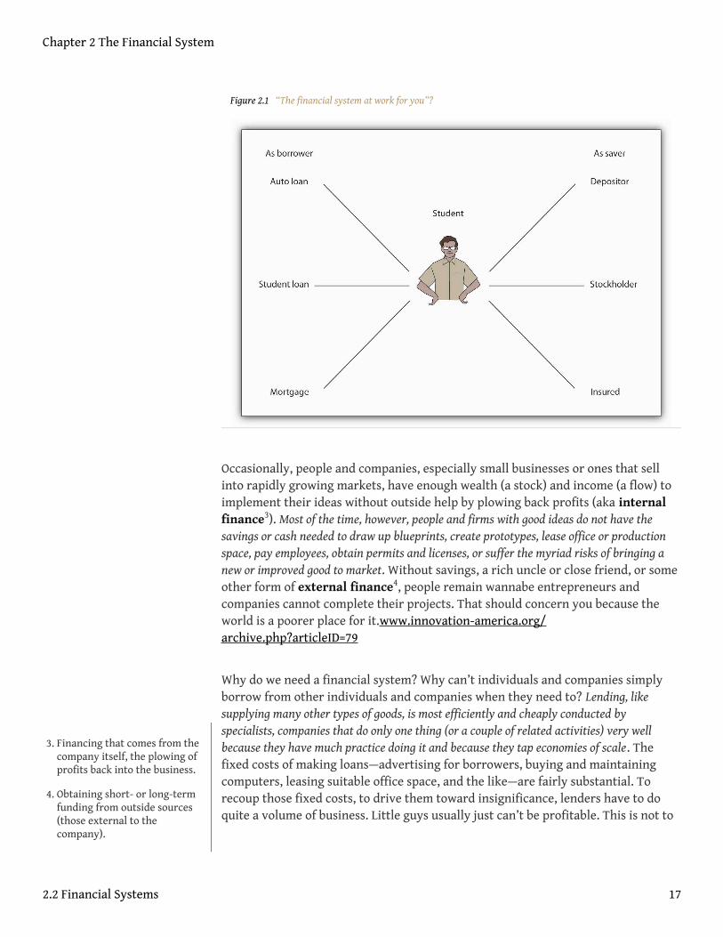
Figure 2.1 “The financial system at work for you”?
Occasionally, people and companies, especially small businesses or ones that sellinto rapidly growing markets, have enough wealth (a stock) and income (a flow) toimplement their ideas without outside help by plowing back profits (aka internalfinance3). Most of the time, however, people and firms with good ideas do not have thesavings or cash needed to draw up blueprints, create prototypes, lease office or productionspace, pay employees, obtain permits and licenses, or suffer the myriad risks of bringing anew or improved good to market. Without savings, a rich uncle or close friend, or someother form of external finance4, people remain wannabe entrepreneurs andcompanies cannot complete their projects. That should concern you because theworld is a poorer place for it.www.innovation-america.org/archive.php?articleID=79
Why do we need a financial system? Why can’t individuals and companies simplyborrow from other individuals and companies when they need to? Lending, likesupplying many other types of goods, is most efficiently and cheaply conducted byspecialists, companies that do only one thing (or a couple of related activities) very wellbecause they have much practice doing it and because they tap economies of scale. Thefixed costs of making loans—advertising for borrowers, buying and maintainingcomputers, leasing suitable office space, and the like—are fairly substantial. Torecoup those fixed costs, to drive them toward insignificance, lenders have to doquite a volume of business. Little guys usually just can’t be profitable. This is not to
3. Financing that comes from thecompany itself, the plowing ofprofits back into the business.
4. Obtaining short- or long-termfunding from outside sources(those external to thecompany).
Chapter 2 The Financial System
2.2 Financial Systems 17

say, however, that bigger is always better, only that to be efficient financialcompanies must exceed minimum efficient scale5.
KEY TAKEAWAYS
• The financial system is a dense network of interrelated markets andintermediaries that allocates capital and shares risks by linking savers tospenders, investors to entrepreneurs, lenders to borrowers, and therisk-averse to risk-takers.
• It also increases gains from trade by providing payment services andfacilitating intertemporal trade.
• A financial system is necessary because few businesses can rely oninternal finance alone.
• Specialized financial firms that have achieved minimum efficient scaleare better at connecting investors to entrepreneurs than nonfinancialindividuals and companies.
5. The smallest a business can beand still remain efficient and/or profitable.
Chapter 2 The Financial System
2.2 Financial Systems 18
2.3 Asymmetric Information: The Real Evil
LEARNING OBJECTIVE
1. What is asymmetric information, what problems does it cause, and whatcan mitigate it?
Finance also suffers from a peculiar problem that is not easily overcome by just anybody.Undoubtedly, you’ve already encountered the concept of opportunity costs, thenasty fact that to obtain X you must give up Y, that you can’t have your cake and eatit too. You may not have heard of asymmetric information, another nasty fact thatmakes life much more complicated. Like scarcity6, asymmetric information inheresin nature, the devil incarnate. That is but a slight exaggeration. When a seller(borrower, a seller of securities) knows more than a buyer (lender or investor, abuyer of securities), only trouble can result. Like the devil in Dante’sInferno,http://www.fullbooks.com/Dante-s-Inferno.html this devil has two big uglyheads, adverse selection7, which raises Cain before a contract is signed, and moralhazard8, which entails sinning after contract consummation. (Later, we’ll learnabout a third head, the principal-agency problem, a special type of moral hazard.)
Due to adverse selection, the fact that the riskiest borrowers are the ones who moststrongly desire loans, lenders attract sundry rogues, knaves, thieves, and ne’er-do-wells, like pollen-laden flowers attract bees (Natty Lightwww.urbandictionary.com/define.php?term=natty+light attracts frat boys?). If they are unaware of that selectionbias, lenders will find themselves burned so often that they will prefer to keep their savingsunder their mattresses rather than risk lending it. Unless recognized and effectivelycountered, moral hazard will lead to the same suboptimal outcome. After a loan hasbeen made, even good borrowers sometimes turn into thieves because they realize that theycan gamble with other people’s money. So instead of setting up a nice little ice creamshop with the loan as they promised, a disturbing number decide instead to try toget rich quick by taking a quick trip to Vegas or AtlanticCitywww.pickeringchatto.com/index.php/pc_site/monographs/gambling_on_the_american_dream for some potentially lucrative fun at theblackjack table. If they lose, they think it is no biggie because it wasn’t their money.
One of the major functions of the financial system is to tangle with those devilishinformation asymmetries. It never kills asymmetry, but it usually reduces itsinfluence enough to let businesses and other borrowers obtain funds cheaplyenough to allow them to grow, become more efficient, innovate, invent, and expand
6. The finite availability ofresources coupled with theinfinite demand for them; thefact that goods are notavailable in sufficient quantityto satisfy everyone’s wants.
7. The fact that the least desirableborrowers and those who seekinsurance most desire loansand insurance policies.
8. Any postcontractual change inbehavior that injures otherparties to the contract.
Chapter 2 The Financial System
19
into new markets. By providing relatively inexpensive forms of external finance, financialsystems make it possible for entrepreneurs and other firms to test their ideas in themarketplace. They do so by eliminating, or at least reducing, two major constraintson liquidity9 and capital10, or the need for short-term cash and long-termdedicated funds. They reduce those constraints in two major ways: directly (thoughoften with the aid of facilitators11) via markets12 and indirectly viaintermediaries13. Another way to think about that is to realize that the financialsystem makes it easy to trade intertemporally, or across time. Instead ofimmediately paying for supplies with cash, companies can use the financial systemto acquire what they need today and pay for it tomorrow, next week, next month,or next year, giving them time to produce and distribute their products.
Stop and Think Box
You might think that you would never stoop so low as to take advantage of alender or insurer. That may be true, but financial institutions are not worriedabout you per se; they are worried about the typical reaction to asymmetricinformation. Besides, you may not be as pristine as you think. Have you everdone any of the following?
• Stolen anything from work?• Taken a longer break than allowed?• Deliberately slowed down at work?• Cheated on a paper or exam?• Lied to a friend or parent?
If so, you have taken advantage (or merely tried to, if you were caught) ofasymmetric information.
9. The ease, speed, and cost ofsale of an asset.
10. In this context, long-termfinancing.
11. In this context, businesses thathelp markets to function moreefficiently.
12. Institutions where the quantityand price of goods aredetermined.
13. Businesses that connectinvestors to entrepreneurs viavarious financial contracts, likechecking accounts andinsurance policies.
Chapter 2 The Financial System
2.3 Asymmetric Information: The Real Evil 20
KEY TAKEAWAYS
• Asymmetric information occurs when one party knows more about aneconomic transaction or asset than the other party does.
• Adverse selection occurs before a transaction takes place. Ifunmitigated, lenders and insurers will attract the worst risks.
• Moral hazard occurs after a transaction takes place. If unmitigated,borrowers and the insured will take advantage of lenders and insurers.
• Financial systems help to reduce the problems associated with bothadverse selection and moral hazard.
Chapter 2 The Financial System
2.3 Asymmetric Information: The Real Evil 21

Figure 2.2 Nineteenth-century picture of maletelegraph operator
2.4 Financial Markets
LEARNING OBJECTIVE
1. In what ways can financial markets and instruments be grouped?
Financial markets come in a variety of flavors to accommodate the wide array of financialinstruments or securities that have been found beneficial to both borrowers and lenders overthe years. Primary markets are where newly created (issued) instruments are soldfor the first time. Most securities are negotiable. In other words, they can be sold toother investors at will in what are called secondary markets. Stock exchanges, orsecondary markets for ownership stakes in corporations called stocks (aka shares orequities), are the most well-known type, but there are also secondary markets fordebt, including bonds (evidences of sums owed, IOUs), mortgages, and derivatives14
and other instruments. Not all secondary markets are organized as exchanges,centralized locations, like the New York Stock Exchange or the Chicago Board ofTrade, for the sale of securities. Some are over-the-counter (OTC) markets run bydealers15 connected via various telecom devices (first by post and semaphore [flagsignals], then by telegraph, then telephone, and now computer). Completelyelectronic stock markets have gained much ground in recent years.“StockExchanges: The Battle of the Bourses,” The Economist (31 May 2008), 77–79.
Money markets are used to trade instruments with less than ayear to maturity (repayment of principal). Examples includethe markets for T-bills (Treasury bills or short-termgovernment bonds), commercial paper (short-termcorporate bonds), banker’s acceptances (guaranteedbank funds, like a cashier’s check), negotiablecertificates of deposit (large-denomination negotiableCDs, called NCDs), Fed funds (overnight loans ofreserves between banks), call loans (overnight loans onthe collateral of stock), repurchase agreements (short-term loans on the collateral of T-bills), and foreignexchange (currencies of other countries).
Securities with a year or more to maturity trade in capitalmarkets. Some capital market instruments, calledperpetuities, never mature or fall due. Equities(ownership claims on the assets and income of
14. Derivatives are complexfinancial instruments, theprices of which are based onthe prices of underlying assets,variables, or indices. Someinvestors use them to hedge(reduce) risks, while others(speculators) use them toincrease risks.
15. Businesses that buy and sellsecurities continuously at bidand ask prices, profiting fromthe difference or spreadbetween the two prices.
Chapter 2 The Financial System
22
© 2010 JupiterimagesCorporation
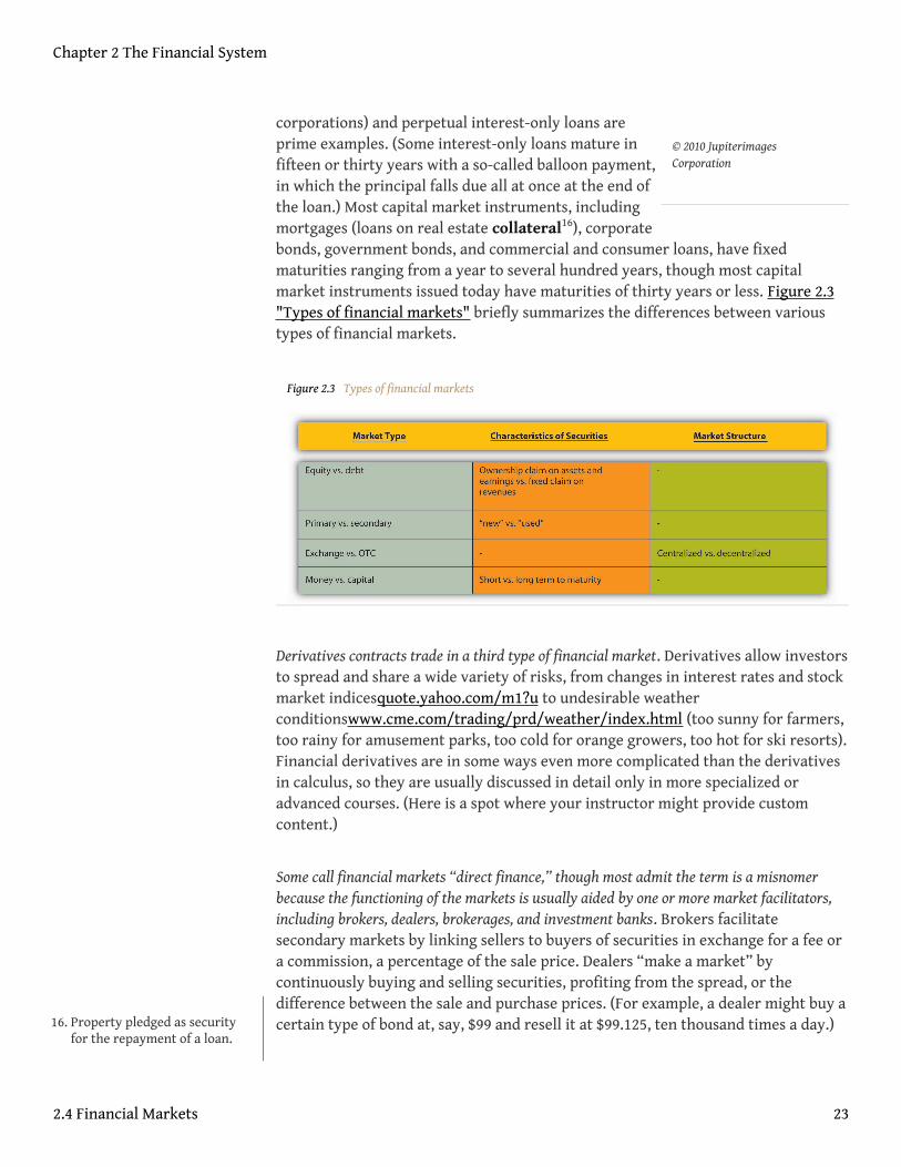
corporations) and perpetual interest-only loans areprime examples. (Some interest-only loans mature infifteen or thirty years with a so-called balloon payment,in which the principal falls due all at once at the end ofthe loan.) Most capital market instruments, includingmortgages (loans on real estate collateral16), corporatebonds, government bonds, and commercial and consumer loans, have fixedmaturities ranging from a year to several hundred years, though most capitalmarket instruments issued today have maturities of thirty years or less. Figure 2.3"Types of financial markets" briefly summarizes the differences between varioustypes of financial markets.
Figure 2.3 Types of financial markets
Derivatives contracts trade in a third type of financial market. Derivatives allow investorsto spread and share a wide variety of risks, from changes in interest rates and stockmarket indicesquote.yahoo.com/m1?u to undesirable weatherconditionswww.cme.com/trading/prd/weather/index.html (too sunny for farmers,too rainy for amusement parks, too cold for orange growers, too hot for ski resorts).Financial derivatives are in some ways even more complicated than the derivativesin calculus, so they are usually discussed in detail only in more specialized oradvanced courses. (Here is a spot where your instructor might provide customcontent.)
Some call financial markets “direct finance,” though most admit the term is a misnomerbecause the functioning of the markets is usually aided by one or more market facilitators,including brokers, dealers, brokerages, and investment banks. Brokers facilitatesecondary markets by linking sellers to buyers of securities in exchange for a fee ora commission, a percentage of the sale price. Dealers “make a market” bycontinuously buying and selling securities, profiting from the spread, or thedifference between the sale and purchase prices. (For example, a dealer might buy acertain type of bond at, say, $99 and resell it at $99.125, ten thousand times a day.)16. Property pledged as security
for the repayment of a loan.
Chapter 2 The Financial System
2.4 Financial Markets 23
Brokerages engage in both brokering and dealing and usually also providing theirclients with advice and information. Investment banks facilitate primary marketsby underwriting stock and bond offerings, including initial public offerings (IPOs) ofstocks, and by arranging direct placements17 of bonds. Sometimes investmentbanks act merely as brokers, introducing securities issuers to investors, usuallyinstitutional investors like the financial intermediaries discussed below. Sometimesthey act as dealers, buying the securities themselves for later (hopefully soon!)resale to investors. And sometimes they provide advice, usually regardingmergers18 and acquisitions19. Investment banks took a beating during the financialcrisis that began in 2007. Most of the major ones went bankrupt or merged withlarge commercial banks. Early reports of the death of investment banking turnedout to be premature, but the sector is depressed at present; two large ones andnumerous small ones, niche players called boutiques, remain.“American Finance:And Then There Were None. What the death of the investment bank means for WallStreet,” The Economist (27 September 2008), 85–86.
Stop and Think Box
In eighteenth-century Pennsylvania and Maryland, people could buy realestate, especially in urban areas, on so-called ground rent, in which theyobtained clear title and ownership of the land (and any buildings or otherimprovements on it) in exchange for the promise to pay some percentage(usually 6) of the purchase price forever. What portion of the financial systemdid ground rents (some of which are still being paid) inhabit? How else mightground rents be described?
Ground rents were a form of market or direct finance. They were financialinstruments or, more specifically, perpetual mortgages akin to interest-onlyloans.
Financial markets are increasingly international in scope. Integration of transatlanticfinancial markets began early in the nineteenth century and accelerated after themid-nineteenth-century introduction of the transoceanic telegraph systems. Theprocess reversed early in the twentieth century due to World Wars I and II and thecold war; the demise of the gold standard;John H. Wood, “The Demise of the GoldStandard,” Economic Perspectives (Nov. 1981): 13-23.economics.about.com/od/foreigntrade/a/bretton_woods.htm system of fixed exchange rates, discretionarymonetary policy, and capital immobility. (We’ll explore these topics and a relatedmatter, the so-called trilemma, or impossible trinity, in Chapter 19 "International
17. A sale of financial securities,usually bonds, via directnegotiations with buyers,usually large institutionalinvestors like insurance andinvestment companies.
18. A merger occurs when two ormore extant business firmscombine into one through apooling of interests or throughpurchase.
19. When one company takes acontrolling interest in another;when one business buysanother.
Chapter 2 The Financial System
2.4 Financial Markets 24
Monetary Regimes".) With the end of the Bretton Woods arrangement in the early1970s and the cold war in the late 1980s/early 1990s, financial globalizationreversed course once again. Today, governments, corporations, and other securitiesissuers (borrowers) can sell bonds, called foreign bonds, in a foreign countrydenominated in that foreign country’s currency. (For example, the Mexicangovernment can sell dollar-denominated bonds in U.S. markets.) Issuers can alsosell Eurobonds or Eurocurrencies, bonds issued (created and sold) in foreigncountries but denominated in the home country’s currency. (For example, U.S.companies can sell dollar-denominated bonds in London and U.S. dollars can bedeposited in non-U.S. banks. Note that the term Euro has nothing to do with theeuro, the currency of the European Union, but rather means “outside.” A Euro loan,therefore, would be a loan denominated in euro but made in London, New York,Tokyo, or Perth.) It is now also quite easy to invest in foreign stockexchanges,www.foreign-trade.com/resources/financel.htm many of which havegrown in size and importance in the last few years, even if they struggled throughthe panic of 2008.
Stop and Think Box
To purchase the Louisiana Territory from Napoleon in 1803, the U.S.government sold long-term, dollar-denominated bonds in Europe. Whatportion of the financial system did those bonds inhabit? Be as specific aspossible.
Those government bonds were Eurobonds because the U.S. government issuedthem overseas but denominated them in U.S. dollars.
KEY TAKEAWAYS
• Financial markets can be categorized or grouped by issuance (primaryvs. secondary markets), type of instrument (stock, bond, derivative), ormarket organization (exchange or OTC).
• Financial instruments can be grouped by time to maturity (money vs.capital) or type of obligation (stock, bond, derivative).
Chapter 2 The Financial System
2.4 Financial Markets 25
2.5 Financial Intermediaries
LEARNING OBJECTIVE
1. In what ways can financial intermediaries be classified?
Like financial markets, financial intermediaries are highly specialized. Sometimescalled the indirect method of finance, intermediaries, like markets, link investors/lenders/savers to borrowers/entrepreneurs/spenders but do so in an ingenious way, by transformingassets20. Unlike facilitators, which, as we have seen, merely broker or buy and sellthe same securities, intermediaries buy and sell instruments with different risk21,return22, and/or liquidity characteristics. The easiest example to understand is thatof a bank that sells relatively low risk (which is to say, safe), low return, and highlyliquid liabilities23, called demand deposits, to investors called depositors and buysthe relatively risky, high return, and nonliquid securities of borrowers in the formof loans, mortgages, and/or bonds. Note, too, that investor–depositors own claimson the bank itself rather than on the bank’s borrowers.
Financial intermediaries are sometimes categorized according to the type of assettransformations they undertake. As noted above, depository institutions, includingcommercial banks, savings banks, and credit unions, issue short-term deposits andbuy long-term securities. Traditionally, commercial banks specialized in issuingdemand, transaction, or checking deposits and making loans to businesses. Savingsbanks issued time or savings deposits and made mortgage loans to households andbusinesses, while credit unions issued time deposits and made consumer loans.(Finance companies also specialize in consumer loans but are not considereddepository institutions because they raise funds by selling commercial paper,bonds, and equities rather than by issuing deposits.)
Due to deregulation24, though, the lines between different types of depository institutionshave blurred in recent years. Ownership structure, charter terms, and regulatoryagencies now represent the easiest way to distinguish between different types ofdepository institutions. Almost all commercial and many savings banks are joint-stock corporations. In other words, stockholders own them. Some savings banksand all credit unions are mutual corporations and hence are owned by those whohave made deposits with them.
Insurance companies are also divided between mutual and joint-stock corporations. Theyissue contracts or policies that mature or come due should some contingency occur, which is
20. Assets are “things owned” asopposed to liabilities, whichare “things owed.”
21. The probability of loss.
22. The percentage gain or lossfrom an investment.
23. Liabilities are “things owed” toothers, as opposed to assets,which are “things owned.”
24. Generally, deregulation refersto any industry whereregulations are eliminated orsignificantly reduced. In thiscontext, deregulation refers toa series of regulatory reformsof the financial industryundertaken in the 1980s and1990s.
Chapter 2 The Financial System
26
a mechanism for spreading and sharing risks. Term life insurance policies pay off if theinsured dies within the contract period, while life annuities pay off if the insured isstill alive. Health insurance pays when an insured needs medical assistance.Property or casualty insurance, such as fire or automobile insurance, comes due inthe event of a loss, like a fire or an accident. Liability insurance pays off whensomeone is sued for a tort (damages). Insurers invest policyholder premiums25 instocks, corporate and government bonds, and various money market instruments,depending on the nature of the contingencies they insure against. Life insurancecompanies, for example, invest in longer-term assets than automobile or healthinsurers because, on average, life insurance claims occur much later than propertyor health claims. (In the parlance of insurance industry insiders, life insurance has amuch longer “tail” than property insurance.)
The third major type of intermediary is the investment company, a category that includespension and government retirement funds, which transform corporate bonds and stocks intoannuities, and mutual funds and money market mutual funds, which transform diverseportfolios of capital and money market instruments, respectively, into nonnegotiable26
but easily redeemable27 “shares.”
As Figure 2.4 "Share of total U.S. financial assets, year-end, 1945–2010"shows, therelative importance of commercial banks and life insurance companies has waned sinceWorld War II due to the proliferation of additional investment options. As Figure 2.5"Assets of financial intermediaries, selected years, 1945–2005" shows, their declineis relative only; the assets of all major types of intermediaries have grown rapidlyover the last six decades. The figures are in current dollars, or dollars not adjustedfor inflation, and the U.S. economy has grown significantly since the war, in nosmall part due to the financial system. Nevertheless, as shown in Figure 2.6"Financial assets to gross domestic product (GDP), 1945–2010", the assets offinancial intermediaries have grown steadily as a percentage of GDP28.
25. In this context, a sum paid foran insurance contract.
26. Nontransferable to thirdparties.
27. In this context, changeable intocash money by the fund.
28. GDP, or gross domesticproduct, is one of severaldifferent measures ofaggregate output, the totalvalue of all final goods andservices produced in aneconomy.
Chapter 2 The Financial System
2.5 Financial Intermediaries 27
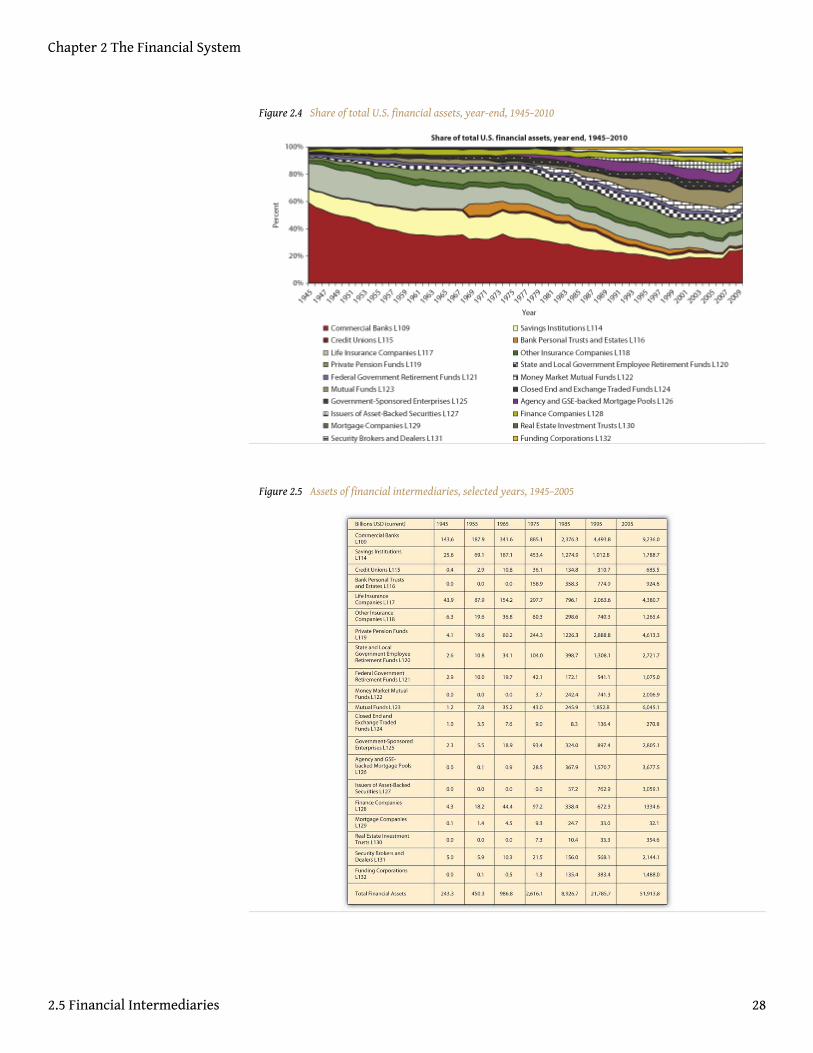
Figure 2.4 Share of total U.S. financial assets, year-end, 1945–2010
Figure 2.5 Assets of financial intermediaries, selected years, 1945–2005
Chapter 2 The Financial System
2.5 Financial Intermediaries 28
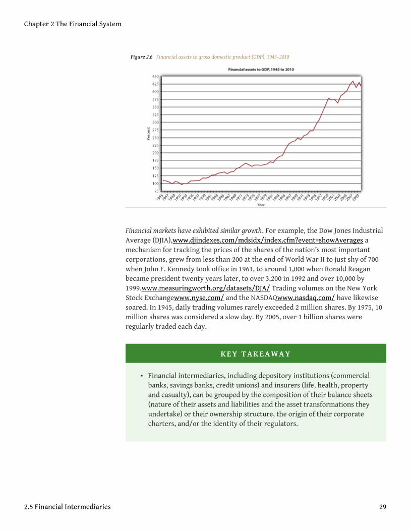
Figure 2.6 Financial assets to gross domestic product (GDP), 1945–2010
Financial markets have exhibited similar growth. For example, the Dow Jones IndustrialAverage (DJIA),www.djindexes.com/mdsidx/index.cfm?event=showAverages amechanism for tracking the prices of the shares of the nation’s most importantcorporations, grew from less than 200 at the end of World War II to just shy of 700when John F. Kennedy took office in 1961, to around 1,000 when Ronald Reaganbecame president twenty years later, to over 3,200 in 1992 and over 10,000 by1999.www.measuringworth.org/datasets/DJA/ Trading volumes on the New YorkStock Exchangewww.nyse.com/ and the NASDAQwww.nasdaq.com/ have likewisesoared. In 1945, daily trading volumes rarely exceeded 2 million shares. By 1975, 10million shares was considered a slow day. By 2005, over 1 billion shares wereregularly traded each day.
KEY TAKEAWAY
• Financial intermediaries, including depository institutions (commercialbanks, savings banks, credit unions) and insurers (life, health, propertyand casualty), can be grouped by the composition of their balance sheets(nature of their assets and liabilities and the asset transformations theyundertake) or their ownership structure, the origin of their corporatecharters, and/or the identity of their regulators.
Chapter 2 The Financial System
2.5 Financial Intermediaries 29
2.6 Competition Between Markets and Intermediaries
LEARNING OBJECTIVE
1. What trade-offs do investors face? How do borrowers decide whether touse financial markets or intermediaries to obtain the funds they need?
Why do investors (savers) sometimes choose to invest in intermediaries rather thandirectly in financial markets? Why do borrowers sometimes choose to reduce theirliquidity and capital constraints via intermediaries and sometimes via markets?Markets and intermediaries often fulfill the same needs, though in different ways.Borrowers/securities issuers typically choose the alternative with the lowest overall cost,while investors/savers choose to invest in the markets or intermediaries that provide themwith the risk-return-liquidity trade-off that best suits them.
Risk is a bad thing, while return and liquidity are good things. Therefore, every saverwants to invest in riskless, easily saleable investments that generate high returns.Of course, such opportunities occur infrequently because investors bid up theirprices, thus reducing their returns. (As we’ll see in Chapter 4 "Interest Rates", thehigher the price of an investment, the lower its return, ceteris paribus29.) To keepreturns high, some investors will be willing to give up some liquidity or to take onmore risk. For example, they might buy securities not backed by collateral (assetslike buildings, businesses, or safe financial instruments like T-bills that theborrower promises to forfeit in case of default30). As a result of the competitionbetween investors, and between borrowers, the financial system offers instrumentswith a wide variety of characteristics, ranging from highly liquid, very safe, butlow-return T-bills and demand deposits, to medium-risk, medium-liquidity,medium-return mortgages, to risky but potentially lucrative and easily soldderivatives like put options and foreign exchange futures contracts.
Investors care about more than risk, return, and liquidity, but generally other considerationsare secondary. For example, investors will pay more for investments with fixedredemption dates rather than ones that can be called (repaid) at the borrower’soption because fixed redemption dates reduce investors’ uncertainty. They will alsosometimes pay a little more for instruments issued by environmentally or sociallyconscious companies and countries and less for those issued by dirty, rude ones.
29. All else equal.
30. Non- or partial payment of aloan, bond, or other paymentobligation.
Chapter 2 The Financial System
30
Stop and Think Box
In the fall of 2006, interest rates on conventional thirty-year home mortgageswithout a prepayment penalty were about 6.5 percent per year. But mortgageswith otherwise identical terms that contained a prepayment penalty for thefirst seven years of the loan could be had for 6.25 percent per year. Why wasthat the case?
In addition to risk, return, and liquidity, investors are concerned about theuncertainty of repayment terms. They are willing to receive a lower return(ceteris paribus, of course) in exchange for a guarantee that a loan will not berepaid for a significant period of time.
As noted above, borrowers also compete with each other for the lowest costmethods of meeting their external financing needs. Obviously, borrowers want topay as little for funds as possible and would like nothing better than to borrow hugesums forever, unconditionally, and at zero interest. Nobody wants to lend on thoseterms, though, so borrowers compete with each other for funds by offeringinvestors higher returns, less risk, or more liquid instruments. They use whicheverpart of the financial system, markets or intermediaries, offers them the best deal. Acompany may sell commercial paper in the money market rather than obtain abank loan, for example, if it is large enough and well-known enough to interestenough investors and market facilitators. A smaller, newer company, though, mayfind that a bank loan is much easier and cheaper to obtain.
KEY TAKEAWAYS
• Investors primarily trade off among risk, return, and liquidity, and to alesser extent they also value the certainty of redemption terms.
• Borrowers want to obtain funds as cheaply as possible and on repaymentterms as flexible as possible.
Chapter 2 The Financial System
2.6 Competition Between Markets and Intermediaries 31
2.7 Regulation
LEARNING OBJECTIVE
1. What are the major goals of financial regulation?
Like investors, borrowers are concerned about the total net costs (all costs plus all benefits)of different types of finance. One big consideration is government and self-regulation.Compared to most other parts of modern capitalist economies, the financial system isrelatively heavily regulated. Regulators like the Securities and Exchange Commission(SEC, which oversees exchanges and OTC markets), the New York Stock Exchange(NYSE, which oversees itself), and the Commodities Futures Trading Commission(CFTC, which oversees futures market exchanges) monitor and regulate financialmarkets. Other regulators, including the Office of the Comptroller of the Currency(which oversees federally chartered commercial banks), the Federal DepositInsurance Corporation (FDIC, which oversees almost all depositories), and sundrystate banking and insurance commissions, monitor financial intermediaries.Companies that wish to avoid direct regulatory scrutiny due to its high cost tend touse intermediaries rather than markets. For example, instead of selling shares tothe public, which would require following the many rules of the SEC and the NYSE(or other exchange or OTC market), a company might decide that it would becheaper to obtain a long-term bank loan or sell bonds to life insurers, mutual funds,and other institutional investors in a direct placement.
Regulators serve four major functions. First, they try to reduce asymmetric informationby encouraging transparency31. That usually means requiring both financialmarkets and intermediaries to disclose accurate information to investors in a clearand timely manner. A second and closely related goal is to protect consumers fromscammers, shysters, and assorted other grifters. Third, they strive to promotefinancial system competition and efficiency by ensuring that the entry and exit offirms is as easy and cheap as possible, consistent with their first two goals. Forexample, new banks can form but only after their incorporators (founders) andinitial executives have been carefully screened. Insurance companies can go out ofbusiness (exit) but only after they have made adequate provision to fulfill theirpromises to policyholders.
Finally, regulators also try to ensure the soundness of the financial system by acting as alender of last resort32, mandating deposit insurance33, and limiting competitionthrough restrictions on entry and interest rates. The first two forms of regulation are
31. In general, the opposite ofopacity. In this context,transparency means arelatively low degree ofasymmetric information.
32. During a financial crisis orpanic, a lender of last resortmakes loans when no one elsewill.
33. Insurance that pays off if abank defaults on its depositliabilities.
Chapter 2 The Financial System
32
generally not controversial, although many believe that the lender of last resortfunction should not be combined with a too big to fail (TBTF) policy34. Limitingcompetition is a highly controversial means of ensuring safety because it extendsprivileges to existing institutions over new ones. Little surprise, then, that theregulated companies themselves are often the strongest supporters of that type ofregulation!
Stop and Think Box
For decades, the Federal Reserve capped the interest rates that banks could payon checking deposits at zero and the interest rates that they could pay on timeor savings deposits at around 6 percent per year. What was the intendedeconomic effect of those restrictions? Why didn’t existing banks lobby for theirrepeal until the Great Inflation35 of the 1970s?
The restrictions were put in place to limit competition among banks, allowingthem to be profitable without assuming too much risk. Existing banks weremore than happy to reap relatively riskless profits until inflation exceeded theinterest rates that they could legally pay. At that point, disintermediation wasrampant. In other words, many people pulled their money out of banks and putthem directly into the market, via money market and stock and bond mutualfunds.
KEY TAKEAWAYS
• Regulators attempt to maximize macroeconomic stability andtransparency and to minimize investor risk and loss.
• The policies they implement to do so, however, can be controversial andare not always effective.34. The notion that some financial
institutions cannot be allowedto go bankrupt because theyowe so much money to somany people and companiesthat their failure to continuemaking payments would havecatastrophic negativeconsequences for the economy.
35. Peacetime inflation rates in theUnited States in the 1970s werehigher than any time before orsince.
Chapter 2 The Financial System
2.7 Regulation 33
2.8 Suggested Reading
Anonymous, Finance for Managers. Cambridge: Harvard Business School Press, 2002.
Barth, James, Gerard Caprio, and Ross Levine. Rethinking Bank Regulation: Till AngelsGovern. New York: Cambridge University Press, 2008.
Bebczuk, Ricardo. Asymmetric Information in Financial Markets: Introduction andApplications. New York: Cambridge University Press, 2003.
Fabozzi, Frank. The Handbook of Financial Instruments. Hoboken, NJ: John Wiley andSons, 2002.
Ferguson, Niall. The Ascent of Money: A Financial History of the World. New York:Penguin Press, 2008.
Landier, Augustin, and Vinay Nair. Investing for Change: Profit from ResponsibleInvestment. New York: Oxford University Press, 2008.
Tyson, Eric. Personal Finance for Dummies, 5th ed. Hoboken, NJ: John Wiley and Sons,2006.
Chapter 2 The Financial System
34
Chapter 3
Money
CHAPTER OBJECTIVES
By the end of this chapter, students should be able to:
1. Define money.2. Describe the work or economic functions that money performs.3. Define barter and explain why it is economically inefficient.4. Explain why some forms of commodity money are better than others.5. Explain why representative money and credit money supplanted
commodity money.6. Define the money supply and explain how and why it is measured.
35
3.1 Of Love, Money, and Transactional Efficiency
LEARNING OBJECTIVE
1. What is money and what economic functions does it perform?
Like love, money is ubiquitous, yet few of us feel that we have enough of either. Asabstract concepts, money and love are both slippery, yet most of us believe that weknow them when we see them. Despite those similarities, mixing money and love can bedangerous. The love of money is said to be one of the seven deadly sins; the money oflove, despite its hoariness, is illegal in many jurisdictions in the United States andabroad.
Jest and wordplay aside, money is, perhaps, the most important invention of all time. Likethe other major contenders for the title, indoor plumbing, internal combustionengines, computers, and other modern gadgets of too recent origin to consider; thewheel, which needs no introduction; the hearth, a pit for controlling fire; and theatlatl, a spear thrower similar in concept to a lacrosse stick, money is a forcemultiplier. In other words, it allows its users to complete much more work in agiven amount of time than nonusers can possibly do, just as the wheel let portersmove more stuff, the hearth helped cooks prepare more food, and the atlatl allowedhunters (warriors) to kill more prey (enemies).
What work does money do? It facilitates trade by making it easier to buy and sell goodscompared to barter, the exchange of one nonmoney good for another. (If you’ve evertraded baseball cards, clothes, beers, phone numbers, homework assignments, orany other nonmoney goods, you’ve engaged in barter.) This is no minor matterbecause trade is the one thing that makes us human. As that great eighteenth-century Scottish economist Adam Smith (and others) pointed out, no other animaltrades with nonrelatives of the same species. The inherent predisposition to trademay explain why humans have relatively large brains and relatively small digestivetracts. Trade certainly explains why humans have more material comforts by farthan any other species on the planet. Each trade that is fairly consummatedenriches both the buyer and the seller. The good feeling people get when they buy(sell) a good is what economists call consumer surplus1 (producer surplus). Bymaking trading relatively easy, money helps to make humanity happier. (Note thatthis is not the same as claiming that wealth makes people happy. Althoughsometimes used synonymously with wealth in everyday speech, money is actually aspecial form of wealth.)
1. In a standard supply anddemand graph, that area abovethe price line and below thedemand curve.
Chapter 3 Money
36
Imagine what life would be like without money. Suppose you try to fill up yourautomobile’s gasoline tank, or take mass transit to school, or acquire any good,without using money (or credit, money’s close cousin). How would you do it? Youwould have to find something that the seller desired. That could take a long timeand quite possibly forever. If you don’t believe me, go to any Craigslistposting,newyork.craigslist.org/about/sites where you will find listings like the onebelow. It’s a fun diversion, but what would this person think is a “fair” trade? A lavalamp and a Grateful Dead poster? Would she give you a ball of yarn in change?
Date: 2006-11-30, 2:37 PM EST
Hello Craigslisters,
I recently moved to NYC and I have no use for the six items pictured below. Startingfrom the upper left going clockwise, I have: a working desk lamp, a hardcover copyof the NY Times best-selling book The Historian, an unused leather-bound photoalbum, a giant bouncy-ball that lights up when it bounces, a pair of goofysunglasses, and a hand-made tribal mask from Mexico.
Make me any offer for any or all of the items, and if it’s fair, we’ll trade.
Answer: Only if you have a lot of time to waste.
In the lingo of economists, by serving as a means or medium of exchange, moneyeliminates one of the major difficulties of barter, fulfilling this mutual or doublecoincidence of wants. And it does it quite well as it zips across the country and theentire globe.
Another serious difficulty with barter helps us to see the second major type of workthat money does. Suppose that the gas station attendant or bus driver wantedchewing gum and you had some. Exchange may still not take place because a crucialquestion remains unanswered: how many sticks of gum is a gallon of gas or a bustrip worth? Ascertaining the answer turns out to be an insurmountable barrier inmost instances. In a money economy, the number of prices equals the number of tradedgoods because each has a money price, the good’s cost in terms of the unit of account. In abarter economy, by contrast, the number of prices equals the number of pairs of goods. So,for example, an economy with just 1,000 goods (a very poor economy indeed) wouldrequire 499,500 different prices! Little wonder, then, that barter economies, whenthey exist, usually produce only ten or so tradable goods, which means about forty-five different prices, each good paired with nine others. By serving as a unit of
Chapter 3 Money
3.1 Of Love, Money, and Transactional Efficiency 37
account, a measuring rod of economic value, money makes price determinationmuch easier.
The unit of account function of money is more abstract than its work as a mediumof exchange and hence is less well understood, but that does not mean that it is lessimportant. To be an effective force multiplier, money has to eliminate both of barter’sbiggest deficiencies. In other words, it has to end the double coincidence of wantsproblem and reduce the number of prices, ideally to one per good. It does theformer by acting as a medium of exchange, something that people acquire not forits own sake but to trade away to another person for something of use. The latter itdoes by serving as a unit of account, as a way of reckoning value. When functioningas a unit of account, money helps us to answer the question, How much is thatworth? much like inches help us to answer, How long is that? or degrees Fahrenheitor Celsius help us to ascertain, What is the temperature of that? By helping us toreckon value, money allows us to easily and quickly compare the economic value ofunlike things, to compare apples and oranges, both literally and figuratively.
Stop and Think Box
After the demise of the Soviet Union, inflation reigned supreme as the Russianruble lost more and more of its value each day. Rubles remained a medium ofexchange, but in many places in Russia, prices and debts began to bedenominated in “bucks.” What were bucks and why did they arise?
Bucks were essentially U.S. dollars, and they were used as a unit of account andstandard of deferred payment, as a way of reckoning value in a stable unit.Physical U.S. dollar-denominated assets, like Federal Reserve notes, were amedium of exchange, but also, in this context, they were a good store of valuebecause they could purchase more rubles each passing day.
Money also works as a store of value and as a standard of deferred compensation.By store of value, economists mean that money can store purchasing power overtime. Of course, many other assets—real estate, financial securities, precious metalsand gems—perform precisely the same function. Storing value, therefore, is notexclusively a trait of money. By standard of deferred compensation, economists meanthat money can be used to denominate a debt, an obligation to make a payment inthe future.
Chapter 3 Money
3.1 Of Love, Money, and Transactional Efficiency 38
To help you to see the different functions of money, consider the followingtransaction:
Customer: How much for a gallon of gasoline? (A)
Attendant: $2.99 (A)
Customer: Great, fill ’er up. (A)
Attendant: Will that be cash (E), check (E), debit (E), or credit (D)?
In the places labeled (A), money is working as a unit of account. The customer istrying to reckon the value of the gasoline, information that the attendant quicklyencapsulates by quoting a money price. The customer just as quickly decides thatshe would rather have the gasoline than the money, or more precisely the othergoods that the money could acquire, and requests the trade. The attendantresponds by inquiring which medium of exchange (E) the customer wishes to use topay for the good. Cash refers to physical currency, like Federal Reserve notes2 orTreasury coins. Check refers to a paper order for the transfer of money from a bankaccount. Debit refers to an electronic order for a transfer from a bank account or aprepaid declining balance debit card. Credit entails the prearranged transfer offunds from the customer’s creditor, a bank or other lender, in exchange for a smallservice fee from the gas stationGas stations and other vendors sometimes chargehigher prices for credit than for cash sales to compensate them for the transactionfee charged by the credit card companies. Most have given up such policies,however, due to competition for customers who found it convenient to chargepurchases at a time before debit cards were widespread and many merchantsrefused to accept checks due to the high moral hazard. (Too many “bounced,” orwere returned, unpaid, for insufficient funds in the customer’s account.) and thecustomer’s promise to repay the lender (and perhaps interest and a yearly fee). Inthe case of the credit transaction, money is working as a standard of deferredpayment (D) because the customer promises to repay the lender the value of the gasat some point in the future. (We will speak of credit money below, but studentsshould not allow the lingo to confuse them. Credit cards and other loans are notmoney per se but rather are ways of obtaining it. The distinction will becomeclearer as your course of study during the semester unfolds.)
Of course, conversations like the one above rarely occur today. Except in New Jerseyand a few other places, people pump their own gas; stations post their prices on bigsigns for all to see; and in addition to dispensing the product, gas pumps handlecredit and debit (and sometimes cash) purchases with ease. Money makes all that
2. Fiat paper money issued byAmerica’s central bank, theFederal Reserve.
Chapter 3 Money
3.1 Of Love, Money, and Transactional Efficiency 39
possible, saving humanity untold hours of waste over the trillions of exchanges completedeach year.
KEY TAKEAWAYS
• Barter entails the exchange of one good for another. It is inefficientbecause it requires satisfaction of the double coincidence of wants(party one must have what party two desires, and vice versa) and pricingproblems (the number of prices of goods equals the number of possiblepairs).
• Perhaps the most important invention of all time, money is anythingthat reduces the transaction costs of barter, anything that is commonlyaccepted as payment or in exchange.
• Money serves as a medium of exchange (physical means of payment),unit of account (measure of economic value), store of value (method ofstoring said value over time), and standard of deferred payment (basisupon which debts are repaid).
Chapter 3 Money
3.1 Of Love, Money, and Transactional Efficiency 40
3.2 Better to Have Had Money and Lost It Than to Have Never Had Moneyat All
LEARNING OBJECTIVE
1. What usually happens when money is absent in an economy?
To further appreciate money’s importance, consider what happens when it isabsent—universal distress, followed quickly by money’s reintroduction or reinvention!After World War I, for example, the German government created too much moneytoo quickly. Hyperinflation, a very rapid rise in the prices of all goods, ensued.Prices increased so fast that workers insisted on being paid twice daily so they couldrun, not walk, to the nearest store to buy food before their hard-earned wagesbecame worthless. Before the hyperinflation, it was said that you could buy awheelbarrow full of food with a purse full of cash. During the hyperinflation, youneeded a wheelbarrow full of cash to purchase a purse full of food. At the end of thedebacle, you kept the wheelbarrow at home lest your most valuable asset, thewheelbarrow, be stolen! At the end of the crisis, the German economy was on abarter basis, but only briefly before currency reforms stopped the inflation andrestored a money economy.
Chapter 3 Money
41
Stop and Think Box
During its most recent financial crisis, in 2001–2002, Argentina faced a severeshortage of its money, called pesos. Private firms responded by setting up giantflea markets where goods were priced and paid for using the firm’s notes,which in most instances were called creditós. The creditós could be used insubsequent flea markets run by the issuing firm but not in markets run byother firms. Creditós had very limited circulation outside the flea markets. Assoon as the peso crisis passed, the firms stopped running flea markets and nolonger honored the creditós they had issued. What happened in Argentina?
A new form of private credit money spontaneously arose to fill the vacuumcreated by the dearth of pesos. Although not as liquid or safe as pesos, creditóswere far superior to barter. The end-game default can be interpreted asseigniorage, the profit the issuers of creditós exacted for providing money tolocal Argentine communities.
In prisons, prisoner-of-war camps, and other settings where money is unavailable,inmates quickly learn the inadequacies of barter firsthand and adopt the best availablecommodity as money—a medium of exchange; unit of account; a store of value; andeven, to the limited extent that credit is available in such circumstances, a standardof deferred payment. Packs of cigarettes often emerge as the commodity money3 ofchoice. (Talk about one’s fortune going up in smoke!) There are good economicreasons for this preference. Although not perfect, cigarettes are a serviceablemedium of exchange. First and foremost, sealed packs of cigarettes are easilyauthenticated because it would be extremely difficult to counterfeit or adulteratethem, especially under prison conditions. Although they differ somewhat frombrand to brand, they are also relatively uniform in quality. If you gave up a bar ofsoap for two packs, you could rest relatively well assured that you were not beingcheated. Second, cigarette packs are divisible, into twenty individual cigarettes, or“loosies,” without giving up much of their ease of authentication. (A loosie is easierto adulterate than a sealed pack, say, by replacing the tobacco with sawdust, but isstill not easy.) Divisibility is important because supply and demand might welldictate an equilibrium price that includes a fraction of a pack, just as it often leadsto prices that are a fraction of a dollar ($), yen (¥), euro (€), or pound (£). Individualcigarettes are also somewhat divisible but only when filterless or when consumed.One might, for instance, sell a good blanket for four packs, two loosies, and fivedrags or puffs.
3. Forms of money that haveintrinsic value as a commodity.
Chapter 3 Money
3.2 Better to Have Had Money and Lost It Than to Have Never Had Money at All 42
Cigarettes also have relatively high value-to-weight and value-to-bulk ratios. Inother words, they are relatively valuable given their size and weight. Thatportability is, of course, important to their function as a medium of exchange.Although they eventually go stale and can be ruined if smashed or drenched inwater, sealed cigarettes packs are durable enough to also serve as an intermediateterm store of value. The elasticity of the supply of cigarette packs is volatile,however, because smokers find it difficult to quit smoking, no matter the price andthe fact that the quantity of packs in circulation depends on shipments from theoutside world. In modern prisons, this is less of a problem, but in prisoner-of-war(POW) camps, sudden gluts caused the prices of goods (noncigarettes) to soar (thatis, the value of cigarettes plummeted), only to be followed by long periods ofdeflation (lower prices for noncigarettes) as the supply of cigarettes dried up andeach cigarette gained in purchasing power.
KEY TAKEAWAYS
• Where money is absent, an available commodity with the bestcombination of ease of authentication, uniformity, divisibility,durability, portability, and elasticity of supply may emerge as money.
• In other instances, as in Argentina, private credit money may emerge.
Chapter 3 Money
3.2 Better to Have Had Money and Lost It Than to Have Never Had Money at All 43
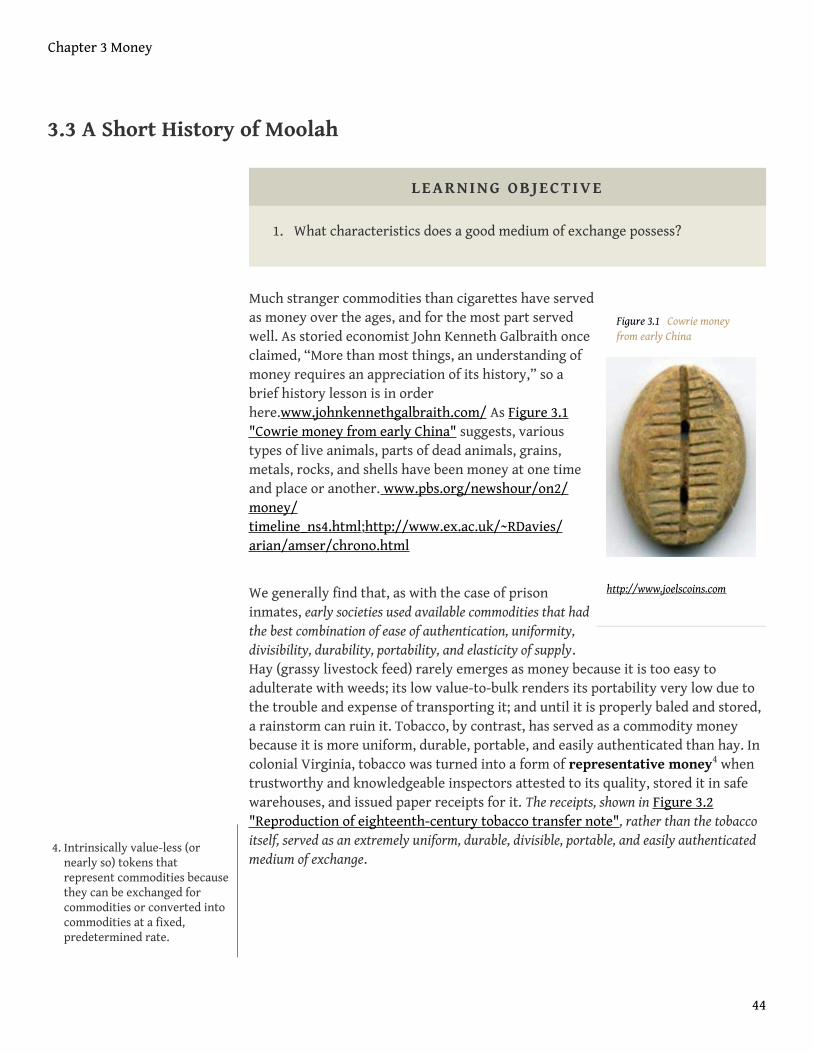
Figure 3.1 Cowrie moneyfrom early China
http://www.joelscoins.com
3.3 A Short History of Moolah
LEARNING OBJECTIVE
1. What characteristics does a good medium of exchange possess?
Much stranger commodities than cigarettes have servedas money over the ages, and for the most part servedwell. As storied economist John Kenneth Galbraith onceclaimed, “More than most things, an understanding ofmoney requires an appreciation of its history,” so abrief history lesson is in orderhere.www.johnkennethgalbraith.com/ As Figure 3.1"Cowrie money from early China" suggests, varioustypes of live animals, parts of dead animals, grains,metals, rocks, and shells have been money at one timeand place or another. www.pbs.org/newshour/on2/money/timeline_ns4.html;http://www.ex.ac.uk/~RDavies/arian/amser/chrono.html
We generally find that, as with the case of prisoninmates, early societies used available commodities that hadthe best combination of ease of authentication, uniformity,divisibility, durability, portability, and elasticity of supply.Hay (grassy livestock feed) rarely emerges as money because it is too easy toadulterate with weeds; its low value-to-bulk renders its portability very low due tothe trouble and expense of transporting it; and until it is properly baled and stored,a rainstorm can ruin it. Tobacco, by contrast, has served as a commodity moneybecause it is more uniform, durable, portable, and easily authenticated than hay. Incolonial Virginia, tobacco was turned into a form of representative money4 whentrustworthy and knowledgeable inspectors attested to its quality, stored it in safewarehouses, and issued paper receipts for it. The receipts, shown in Figure 3.2"Reproduction of eighteenth-century tobacco transfer note", rather than the tobaccoitself, served as an extremely uniform, durable, divisible, portable, and easily authenticatedmedium of exchange.
4. Intrinsically value-less (ornearly so) tokens thatrepresent commodities becausethey can be exchanged forcommodities or converted intocommodities at a fixed,predetermined rate.
Chapter 3 Money
44
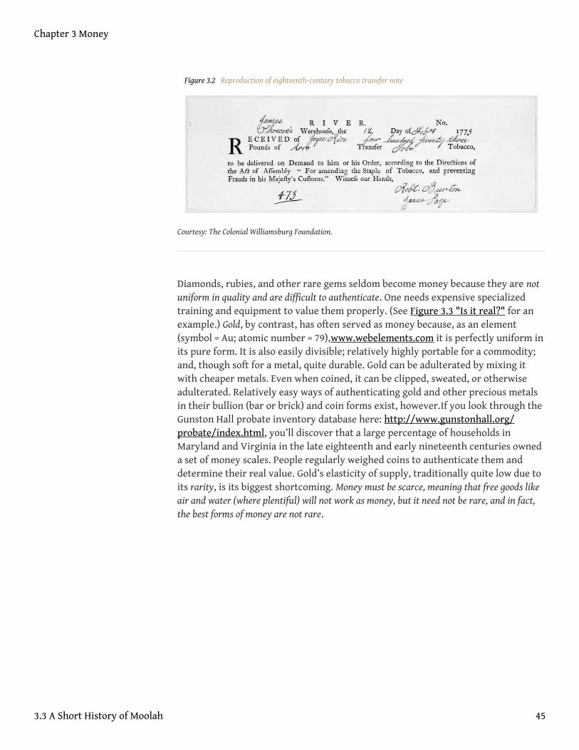
Figure 3.2 Reproduction of eighteenth-century tobacco transfer note
Courtesy: The Colonial Williamsburg Foundation.
Diamonds, rubies, and other rare gems seldom become money because they are notuniform in quality and are difficult to authenticate. One needs expensive specializedtraining and equipment to value them properly. (See Figure 3.3 "Is it real?" for anexample.) Gold, by contrast, has often served as money because, as an element(symbol = Au; atomic number = 79),www.webelements.com it is perfectly uniform inits pure form. It is also easily divisible; relatively highly portable for a commodity;and, though soft for a metal, quite durable. Gold can be adulterated by mixing itwith cheaper metals. Even when coined, it can be clipped, sweated, or otherwiseadulterated. Relatively easy ways of authenticating gold and other precious metalsin their bullion (bar or brick) and coin forms exist, however.If you look through theGunston Hall probate inventory database here: http://www.gunstonhall.org/probate/index.html, you’ll discover that a large percentage of households inMaryland and Virginia in the late eighteenth and early nineteenth centuries owneda set of money scales. People regularly weighed coins to authenticate them anddetermine their real value. Gold’s elasticity of supply, traditionally quite low due toits rarity, is its biggest shortcoming. Money must be scarce, meaning that free goods likeair and water (where plentiful) will not work as money, but it need not be rare, and in fact,the best forms of money are not rare.
Chapter 3 Money
3.3 A Short History of Moolah 45
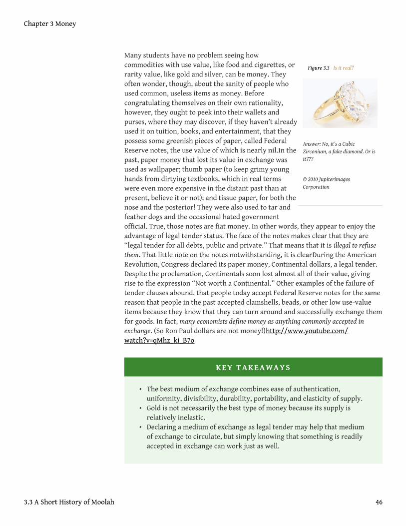
Figure 3.3 Is it real?
Answer: No, it’s a CubicZirconium, a fake diamond. Or isit???
© 2010 JupiterimagesCorporation
Many students have no problem seeing howcommodities with use value, like food and cigarettes, orrarity value, like gold and silver, can be money. Theyoften wonder, though, about the sanity of people whoused common, useless items as money. Beforecongratulating themselves on their own rationality,however, they ought to peek into their wallets andpurses, where they may discover, if they haven’t alreadyused it on tuition, books, and entertainment, that theypossess some greenish pieces of paper, called FederalReserve notes, the use value of which is nearly nil.In thepast, paper money that lost its value in exchange wasused as wallpaper; thumb paper (to keep grimy younghands from dirtying textbooks, which in real termswere even more expensive in the distant past than atpresent, believe it or not); and tissue paper, for both thenose and the posterior! They were also used to tar andfeather dogs and the occasional hated governmentofficial. True, those notes are fiat money. In other words, they appear to enjoy theadvantage of legal tender status. The face of the notes makes clear that they are“legal tender for all debts, public and private.” That means that it is illegal to refusethem. That little note on the notes notwithstanding, it is clearDuring the AmericanRevolution, Congress declared its paper money, Continental dollars, a legal tender.Despite the proclamation, Continentals soon lost almost all of their value, givingrise to the expression “Not worth a Continental.” Other examples of the failure oftender clauses abound. that people today accept Federal Reserve notes for the samereason that people in the past accepted clamshells, beads, or other low use-valueitems because they know that they can turn around and successfully exchange themfor goods. In fact, many economists define money as anything commonly accepted inexchange. (So Ron Paul dollars are not money!)http://www.youtube.com/watch?v=qMhz_ki_B7o
KEY TAKEAWAYS
• The best medium of exchange combines ease of authentication,uniformity, divisibility, durability, portability, and elasticity of supply.
• Gold is not necessarily the best type of money because its supply isrelatively inelastic.
• Declaring a medium of exchange as legal tender may help that mediumof exchange to circulate, but simply knowing that something is readilyaccepted in exchange can work just as well.
Chapter 3 Money
3.3 A Short History of Moolah 46
3.4 Commodity and Credit Monies
LEARNING OBJECTIVE
1. How do representative and credit monies compare to commoditymonies?
Truth be told, the people who used lion teeth or rocks with holes in them as moneymight find moderns a bit off their rockers for using money created by thegovernment. The reason is simple: commodity monies are self-equilibrating, butgovernment fiat monies are not because they are sometimes subject more to the whimsof politicians and bureaucrats than to the forces of supply and demand, as we willsee in Chapter 13 "Central Bank Form and Function". Commodity money systemscan self-equilibrate, or essentially run themselves, because commodities are scarce(but as noted above, not necessarily rare). In other words, the opportunity costs oftheir acquisition and production are greater than zero. That means that at somepoint people will find it just as profitable to produce nonmonetary goods as toproduce money directly. At that point, money creation naturally ceases until moreis needed.
Suppose, for example, that clams are money and that ten can be found in one hour,on average. Suppose too that people on average can also produce a bow in twohours, an arrow in one hour, and a dead rabbit in three hours. In that situation, anarrow would cost ten clams, a bow twenty clams, and a rabbit thirty clams becauseat those prices people would be indifferent whether they spent, say, six hourscollecting clams (6 × 10 = 60), making arrows (6 × 10 = 60), making bows ([6/2 hoursper bow] = 3 bows produced in 6 hours; 3 × 20 = 60), or hunting rabbits ([6/3] = 2; 2 ×30 = 60). If a big clambake takes clams out of (monetary) circulation by putting themin (bloodstream via the digestive tract) circulation, it will be more remunerative toharvest clams than to make bows or arrows or to fricassee rabbits until the supplyof clams is restored, which should not be long. (In fact, if people expected theclambake, the adjustment might well be instantaneous. We’ll discuss theimportance of expectations in Chapter 7 "Rational Expectations, Efficient Markets,and the Valuation of Corporate Equities" and Chapter 26 "Rational ExpectationsRedux: Monetary Policy Implications".)
Commodity money systems also automatically adjust to structural changes in theeconomy. If it suddenly became easier to find clams, say, twenty in an hour,everybody would harvest clams until the clam prices of arrows, bows, and rabbits
Chapter 3 Money
47
doubled, restoring equilibrium. If clam production dropped to five an hour, priceswould also drop by half because no one would harvest clams when they could earntwice as many clams in an hour producing arrows, bows, or rabbits. If clamproduction remained steady but it became easier to produce bows, the only thingthat would change would be the price of bows relative to the prices of arrows andrabbits, and not the price level, or all prices. For example, if it was possible toproduce bows in 1.5 hours instead of 2, the price of bows would drop to 15 clams(when 10 clams can be harvested in an hour).
As noted above, gold is a very good commodity money in most respects. It fell fromgrace early in the twentieth century, however, primarily because of competitionfrom superior types of exchange medium and the inelasticity of its supply. Whengold became more abundant and output remained constant, the price levelincreased because there was more money chasing the same amount of goods andservices. When the quantity of gold remained constant and output increased, theprice level declined because there was no longer enough gold around to maintainthe former prices, as in Figure 3.5 "A higher price for gold means a lower price foreverything else". By making each ounce of gold more valuable, thus increasingone’s ability to purchase more goods and services than formerly, the decline inprices should have triggered an immediate increase in gold production, therebyrendering the deflation, or reduction of the price level, mild and transitory, as inour hypothetical clam case above. Due to the difficulty of finding new veins of gold,however, changes in the price level were often prolonged.This chart depictschanges in the price level in the United States between 1865 and 1900, when thecountry’s unit of account was defined in gold. Note that prices fell in most years.That deflation led to a series of political upheavals that resulted in the formation ofthe Populist Party and a prolonged struggle among Silverites, who desired to raiseprices by monetizing silver; Greenbackers, who sought to raise prices through theissuance of fiat money; and Gold Bugs, who insisted on maintenance of the statusquo. The Wonderful Wizard of Oz, a children’s book by Frank Baum made legendary bya movie version starring Judy Garland as protagonist Dorothy, is an allegorydepicting the major political divisions of the era. Oz is of course the abbreviationfor ounce; the yellow brick road refers to the gold standard; the Emerald Citysymbolizes Greenbacks; and in the book, Dorothy’s slippers were silver, not ruby, asthey were depicted in the movie.
Chapter 3 Money
3.4 Commodity and Credit Monies 48
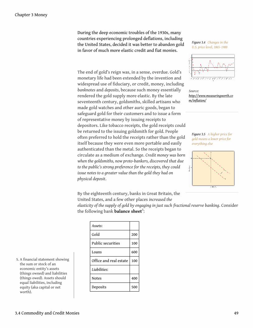
Figure 3.4 Changes in theU.S. price level, 1865–1900
Source:http://www.measuringworth.com/inflation/
Figure 3.5 A higher price forgold means a lower price foreverything else
During the deep economic troubles of the 1930s, manycountries experiencing prolonged deflations, includingthe United States, decided it was better to abandon goldin favor of much more elastic credit and fiat monies.
The end of gold’s reign was, in a sense, overdue. Gold’smonetary life had been extended by the invention andwidespread use of fiduciary, or credit, money, includingbanknotes and deposits, because such money essentiallyrendered the gold supply more elastic. By the lateseventeenth century, goldsmiths, skilled artisans whomade gold watches and other auric goods, began tosafeguard gold for their customers and to issue a formof representative money by issuing receipts todepositors. Like tobacco receipts, the gold receipts couldbe returned to the issuing goldsmith for gold. Peopleoften preferred to hold the receipts rather than the golditself because they were even more portable and easilyauthenticated than the metal. So the receipts began tocirculate as a medium of exchange. Credit money was bornwhen the goldsmiths, now proto-bankers, discovered that dueto the public’s strong preference for the receipts, they couldissue notes to a greater value than the gold they had onphysical deposit.
By the eighteenth century, banks in Great Britain, theUnited States, and a few other places increased theelasticity of the supply of gold by engaging in just such fractional reserve banking. Considerthe following bank balance sheet5:
Assets:
Gold 200
Public securities 100
Loans 600
Office and real estate 100
Liabilities:
Notes 400
Deposits 500
5. A financial statement showingthe sum or stock of aneconomic entity’s assets(things owned) and liabilities(things owed). Assets shouldequal liabilities, includingequity (aka capital or networth).
Chapter 3 Money
3.4 Commodity and Credit Monies 49
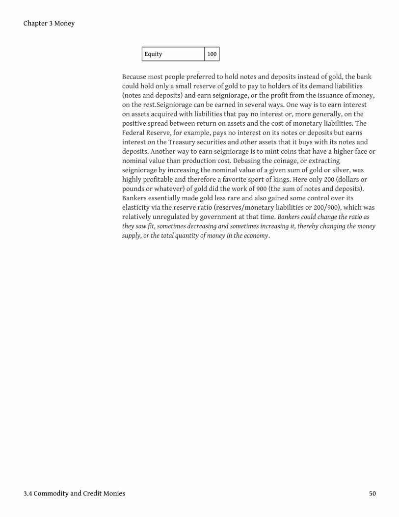
Equity 100
Because most people preferred to hold notes and deposits instead of gold, the bankcould hold only a small reserve of gold to pay to holders of its demand liabilities(notes and deposits) and earn seigniorage, or the profit from the issuance of money,on the rest.Seigniorage can be earned in several ways. One way is to earn intereston assets acquired with liabilities that pay no interest or, more generally, on thepositive spread between return on assets and the cost of monetary liabilities. TheFederal Reserve, for example, pays no interest on its notes or deposits but earnsinterest on the Treasury securities and other assets that it buys with its notes anddeposits. Another way to earn seigniorage is to mint coins that have a higher face ornominal value than production cost. Debasing the coinage, or extractingseigniorage by increasing the nominal value of a given sum of gold or silver, washighly profitable and therefore a favorite sport of kings. Here only 200 (dollars orpounds or whatever) of gold did the work of 900 (the sum of notes and deposits).Bankers essentially made gold less rare and also gained some control over itselasticity via the reserve ratio (reserves/monetary liabilities or 200/900), which wasrelatively unregulated by government at that time. Bankers could change the ratio asthey saw fit, sometimes decreasing and sometimes increasing it, thereby changing the moneysupply, or the total quantity of money in the economy.
Chapter 3 Money
3.4 Commodity and Credit Monies 50
Stop and Think Box
In Ithaca, New York, and hundreds of other communities worldwide, consortiaof businesses issue zero-interest bearer paper notes. The notes aredenominated in local units (Hours in Ithaca; Greenbacks, Berkshares, and othernames elsewhere)http://en.wikipedia.org/wiki/Local_currency#Modern_local_currencies and are designed to circulate as cash,like Federal Reserve notes. In the United States, the issuer must redeem thenotes for dollars (unit of account) upon demand at a fixed conversion rate. EachIthaca Hour, for example, is equal to 10 USD. The community notes are not alegal tender, have no intrinsic value, and generally circulate in an extremelylimited geographical area. The issuers often use Marxist rhetoric, claiming thatholding the notes will help the local economy by keeping money investedlocally. (For more details, browse http://www.ithacahours.com/). What isreally going on in Ithaca and the other community money centers?
The issuers of the notes are interested in earning seigniorage, or profits fromthe issuance of money. They act like fractional reserve bankers, issuing Hoursin exchange for dollars, which they put out to interest. They don’t earn much,though, because most people are smart enough to realize their credit money isless liquid and more risky than other forms of credit money, like bank deposits,and much higher risk than fiat money, like Federal Reserve Notes. In fact, thereis no good reason to hold such notes unless one believes (“buys into”) thedubious Marxist rhetoric that often accompanies them.
Since its invention, credit money has been extremely successful because it is an almostperfect medium of exchange. Take, for example, bank deposits. Essentially just anaccounting entry crediting so much money (unit of account) to a person ororganization, deposits are easily authenticated, perfectly uniform, divisible tofractions of a penny, highly portable via written or electronic orders, and extremelydurable. Moreover, their supply is highly elastic because they can be created anddestroyed at will. The usefulness of deposits is further extended by varying theircharacteristics to meet different risk, return, liquidity, and maturity preferences.The most common and familiar type of deposit, called a checking, transaction, ordemand deposit account, pays no or relatively low interest, but funds can bewithdrawn at any time via teller during banking hours, via ATM 24/7, or with adebit card or check. Other deposits, called time or savings deposits or certificates ofdeposit, pay relatively high interest but either cannot be withdrawn at all before aprespecified date or can be withdrawn only if the depositor suffers a penalty thatwipes out much of the interest earned. Between those two extremes have emerged a
Chapter 3 Money
3.4 Commodity and Credit Monies 51
variety of hybrids, like automatic transfer from savings (ATS)6, and sweepaccounts7, and money market mutual funds8. Most forms of electronic or e-money, like sQuidcards,http://www.squidcard.com/corporate/emoney.html arejust new forms of credit money.
The biggest problem with credit money is that the issuer may default. Many bankingregulations, as we will see in Chapter 11 "The Economics of Financial Regulation",attempt to minimize that risk. Other issuers of credit money are not so closelyregulated, however, and hence constitute serious credit risks9 for holders of theirliabilities.
KEY TAKEAWAYS
• Representative money and credit money are more efficient thancommodity money because they are superior media of exchange andunits of account. Their quality is more uniform and easily ascertained,they have low weight-to-value ratios, they are more divisible and theirdivisibility is more flexible, and their supply is more elastic.
• However, the supply of representative and credit monies generally doesnot self-equilibrate the way the supply of a commodity money does.
6. An account that automaticallymoves funds from your savingsaccount if your checkingaccount is depleted. (Of course,such an account doesn’t help ifyou don’t have any money inyour savings account either.)
7. An account that automaticallymoves funds from your savingsaccount if your checkingaccount is depleted. (Of course,such an account doesn’t help ifyou don’t have any money inyour savings account either.)
8. MMMFs are mutual funds thatinvest in short-term, or moneymarket, instruments. Fundowners earn the going marketinterest rates, minusmanagement fees, and candraw upon their shares bycheck but at a cost higher thanthat of most bank checkingaccounts.
9. The probability of not beingpaid a sum due.
Chapter 3 Money
3.4 Commodity and Credit Monies 52

3.5 Measuring Money
LEARNING OBJECTIVE
1. What is the money supply and how is it measured?
Due in part to the profusion of different types of credit money, measuring the money supplytoday is no easy task. The Fed, or Federal Reserve System, America’s monetaryauthority and central bank, has therefore developed a number of monetaryaggregates, or different measures of the money supply. The monetary base (MB orM0, the narrowest aggregate) is the unweighted total of Federal Reserve notes andTreasury coins in circulation, plus bank reserves (deposits with the FederalReserve). M1 adds to M0 travelers’ checks and demand deposits. (Banks other thanthe Fed no longer issue notes. If they did, they would be considered components ofM1.) A broader aggregate, M2, includes M1 as well as time/savings deposits andretail money market mutual fund shares. A yet broader aggregate, M3, includes M2as well as institutional time deposits, money market mutual fund shares,repurchase agreements, and Eurodollars, but its publication was discontinued bythe Fed in 2006.
The Fed continues to estimate the other three measures because their movementsare not highly correlated and the appropriate monetary aggregate varies over timeand question. As we will see, the money supply helps to determine importantmacroeconomic variables like inflation, unemployment, and interest rates.Accurately measuring the money supply is so important that monetary economistsstill search for better ways of doing it. One approach, called divisia after its Frenchinventor, François Divisia (1925), weighs credit instruments by their liquidity, or inother words, their degree of money-ness, or ease of use as a medium of exchange.The Federal Reserve Bank of Saint Louis tracks the U.S. money supply using variousdivisia formulas.research.stlouisfed.org/msi/
Each Friday, the Wall Street Journal publishes the M1 and M2 monetary aggregates inits “Federal Reserve Data” column. The data is also available on the FederalReserve’s Web site: http://www.federalreserve.gov/releases/h6/. Students arecautioned, however, that the published data are mere estimates; the Fed often revises thefigures by as much as 2 or 3 percent. Other countries’ central banks also report theirmonetary aggregates. Links to the Web sites of other central banks can be foundhere: http://www.bis.org/cbanks.htm.
Chapter 3 Money
53
KEY TAKEAWAYS
• The money supply is the stock of all money in an economy.• It is measured in a variety of ways to aid in the conduct of monetary
policy and in macroeconomic forecasting.
Chapter 3 Money
3.5 Measuring Money 54
3.6 Suggested Reading
Bernstein, Peter. A Primer on Money, Banking, and Gold. Hoboken, NJ: John Wiley andSons, 2008.
Davies, Glyn. A History of Money: From Ancient Times to the Present Day. Cardiff:University of Wales Press, 2002.
Eagleton, Catherine, Jonathan Williams, Joe Cribb, Elizabeth Errington,. Money: AHistory. Richmond Hill, Ontario, Canada: Firefly Books, 2007.
Chapter 3 Money
55
Chapter 4
Interest Rates
CHAPTER OBJECTIVES
By the end of this chapter, students should be able to:
1. Define interest and explain its importance.2. Write and explain the present value formula.3. Write and explain the future value formula.4. Calculate present and future value for multiple periods with annual and
more frequent compounding.5. Define and price major types of debt instruments including discount
bonds, simple loans, fixed payment loans, and coupon bonds.6. Define yield to maturity and identify the types of financial instruments
for which it is relatively easy to calculate.7. Explain why bond prices move inversely to market interest rates.8. Explain why some bond prices are more volatile than others.9. Define rate of return and explain how it differs from yield to maturity.
10. Explain the difference between real and nominal interest rates.
56
4.1 The Interest of Interest
LEARNING OBJECTIVE
1. What is interest and why is it important?
Interest1, the opportunity cost of money, is far from mysterious, but it warrants our carefulconsideration because of its importance. Interest rates2, the price of borrowing money, arecrucial determinants of the prices of assets, especially financial instruments like stocks andbonds, and general macroeconomic conditions, including economic growth3. In fact,ceteris paribus4 (like your grades!) the probability of you landing a job upongraduation will depend in large part on prevailing interest rates. If rates are low,businesses will be more likely to borrow money, expand production, and hire you. Ifrates are high, businesses will be less likely to expand or to hire you. Without a job,you’ll be forced to move back home. Best to pay attention then!
Interest can be thought of as the payment it takes to induce a lender to part withhis, her, or its money for some period of time, be it a day, week, month, year,decade, or century. To make comparisons between those payments easier, interestis almost always expressed as an annual percentage rate, the number of dollars (orother currency)http://fx.sauder.ubc.ca/currency_table.html paid for the use of$100 per year. Several ways of measuring interest rates exist, but here you’ll learn onlyyield to maturity5, the method preferred by economists for its accuracy. The key is tolearn to compare the value of money today, called present value6 (representedhere by the variable PV and aka present discounted value or price), to the value ofmoney tomorrow, called future value7 (represented here by the variable FV).
KEY TAKEAWAYS
• Interest is the opportunity cost of lending money or the price ofborrowing it and can be thought of as the payment a borrower needs toinduce him, her, or it to lend.
• Interest is important because it helps to determine the price of assets,especially financial assets, and to determine various macroeconomicvariables, including aggregate output.
1. The opportunity cost of money.
2. The price of borrowed money.
3. Real per capita GDP.
4. All else equal.
5. The most economicallyaccurate way of measuringinterest rates.
6. The value of money today.
7. The value of money at somepoint in the future.
Chapter 4 Interest Rates
57
4.2 Present and Future Value
LEARNING OBJECTIVE
1. What are the formulas for present value and future value, and whattypes of questions do they help to answer?
A moment’s reflection should convince you that money today is alwaysCertain interestrates occasionally turn very slightly (−0.004%) negative. The phenomenon is so rareand minor that it need not detain us here.worth more than money tomorrow. If youdon’t believe me, send me all of your money immediately. I’ll return every cent ofit—scout’s honor—in exactly one year. I won’t hold my breath. You’d be foolishindeed to forgo food, clothes, housing, transportation, and entertainment for a yearfor no remuneration whatsoever. That’s why a dollar today is worth more than adollar tomorrow. (Another reason that a dollar today is worth more than a dollartomorrow is that, in modern economies, for reasons discussed in Chapter 17"Monetary Policy Targets and Goals", prices tend to rise every year. So $100tomorrow will buy fewer goods and services than $100 today will. We will discussthe impact of inflation8 on interest rates more at the end of this chapter. For now,we consider only nominal interest rates9, not real interest rates10.) But what if Itold you that if you gave me $100 today, I’d give you $1,000 in a year? Most lenderswould jump at that offer (provided they thought I would pay as promised and notdefault), but I wouldn’t offer it and neither would most borrowers. In fact, about$110 would be the most I’d be willing to give you in a year for $100 today. That’s aninterest rate of 10 percent ($10/$100 = .1 or 10%), which, as comedian Adam Sandlermight say, is “not too shabby.”www.tsrocks.com/a/adam_sandler_texts/the_chanukah_song.html If we let the loan ride, as they say, capitalizing theinterest or, in other words, paying interest on the interest every year, calledannually compounding11 interest, your $100 investment would grow in value, asshown in Figure 4.1 "The fate of $100 invested at 10%, compounded annually".
8. A sustained increase in theprice level or average prices.
9. The price of borrowing moneyas it is usually stated,unadjusted for inflation.
10. The price of borrowing moneyadjusted for inflation.
11. Earning interest on interest.
Chapter 4 Interest Rates
58
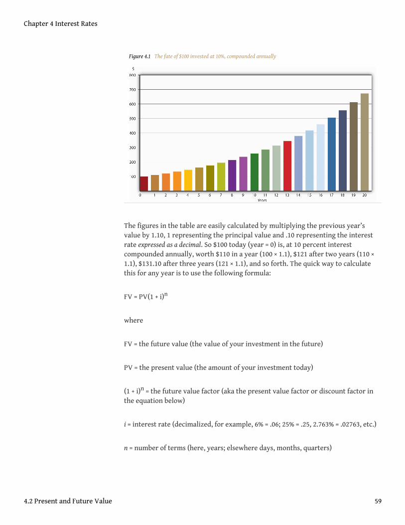
Figure 4.1 The fate of $100 invested at 10%, compounded annually
The figures in the table are easily calculated by multiplying the previous year’svalue by 1.10, 1 representing the principal value and .10 representing the interestrate expressed as a decimal. So $100 today (year = 0) is, at 10 percent interestcompounded annually, worth $110 in a year (100 × 1.1), $121 after two years (110 ×1.1), $131.10 after three years (121 × 1.1), and so forth. The quick way to calculatethis for any year is to use the following formula:
FV = PV(1 + i)n
where
FV = the future value (the value of your investment in the future)
PV = the present value (the amount of your investment today)
(1 + i)n = the future value factor (aka the present value factor or discount factor inthe equation below)
i = interest rate (decimalized, for example, 6% = .06; 25% = .25, 2.763% = .02763, etc.)
n = number of terms (here, years; elsewhere days, months, quarters)
Chapter 4 Interest Rates
4.2 Present and Future Value 59
For $100 borrowed today at 10 percent compounded annually, in 100 years I’d oweyou $1,378,061 (FV = 100 × 1.1100). (Good luck collecting that one!)
What if someone offers to pay you, say, $1,000 in 5 years? How much would you bewilling to pay today for that? Clearly, something less than $1,000. Instead of takinga PV and expanding it via multiplication to determine an FV, here you must do theopposite, or in other words, reduce or “discount” an FV to a PV. You do so bydividing, as in the following formula:
Obviously, we can’t solve this equation unless one of the two remaining variables isgiven. If the interest rate is given as 5 percent, you would pay $783.53 today for$1,000 payable in 5 years (PV = 1000/1.055). If it is 20 percent, you’d give only$401.88 (PV = 1000/1.25). If it is 1 percent, you would give $951.47 (PV = 1000/1.015).Notice that as the interest rate rises (falls), the price of the bond falls (rises). In other words,the price of some future payment (some FV; generically, a bond) and the rate of interest areinversely related. You can see this algebraically by noting that the i term is in thedenominator, so as it gets larger, PV must get smaller (holding FV constant, ofcourse). Economically this makes sense because a higher interest rate means ahigher opportunity cost for money, so a sum payable in the future is worth less themore dear money is.
If payment of the bond described just above were to be made in ten years instead offive, at 1 percent interest per year, you’d pay $905.29 (PV = 1000/1.0110). Note herethat, holding the interest rate (and all other factors) constant, you give less todayfor a payment further in the future ($905.29 < $951.47). That too makes good sensebecause you’re without your money longer and need to be compensated for it bypaying a lower price for the bond/promise/IOU today.
PV = FV/(1 + i)n
or PV = 1000/(1 + i)5
Chapter 4 Interest Rates
4.2 Present and Future Value 60
Stop and Think Box
Congratulations, you just won the Powerball: $100 million payable in $5 millioninstallments over 20 years! Did you really win $100 million? (Hint: Calculate thePV of the final payment with interest at 4 percent.)
No; 5 × 20 = 100, but the money payable next year and in subsequent years is notworth $5 million today if interest rates are above 0, and they almost always are.For example, the last payment, with interest rates at 4 percent compoundedannually, has a PV of only 5,000,000/(1.04)20 = $2,281,934.73.
This is a great place to stop and drill until calculating present value and futurevalue becomes second nature to you. Work through the following problems until ithurts. Then do them again, standing on your head or on one leg.
Chapter 4 Interest Rates
4.2 Present and Future Value 61
EXERCISES
For all questions in this set, interest compounds annually and there are notransaction fees, defaults, etc.
1. On your seventieth birthday, you learn that your grandma, bless hersoul, deposited $50.00 for you on the day of your birth in a savingsaccount bearing 5 percent interest. How much is in the account?
2. You won $1 million in the lottery but unfortunately the money ispayable in a year and you want to start spending it right away. Ifinterest is at 8 percent, how much can you receive today in exchange forthat $1 million in year?
3. As a college freshman, you hoped to save $2,500 to “pimp your ride” as acollege graduation present to yourself. You put $2,012.98 from your highschool graduation haul in the bank at 5 percent interest. Will you meetyour goal?
4. You’ve won a scholarship for your senior year worth $1,500, but it ispayable only after graduation, a year hence. If interest is at 15 percent,how much is your scholarship worth today?
5. You determine that you need $1,750,000 saved in order to retirecomfortably. When you turn 25, you inherit $350,017. If you invest thatsum immediately at 4.42 percent, can you retire at age 65 if you have noother savings?
6. You own two bonds, each with a face, or payoff, value of $1,000. One fallsdue in exactly one year and the other in exactly three years. If interest isat 2.35 percent, how much are those bonds worth today? What if interestrates jump to 12.25 percent?
7. To purchase a car, you borrowed $10,000 from your brother. You offeredto pay him 8 percent interest and to repay the loan in exactly threeyears. How much will you owe your bro?
8. As part of a lawsuit settlement, a major corporation offers you $100,000today or $75,000 next year. Which do you choose if interest rates are 5percent? If they are 13.47886 percent?
9. Exactly 150 years ago, the U.S. government promised to pay a certainIndian tribe $3,500, or 7 percent interest until it did so. Somehow, theaccount was unpaid. How much does the government owe the tribe forthis promise?
10. As part of an insurance settlement, you are offered $100,000 today or$125,000 in five years. If the applicable interest rate is 1 percent, whichoption do you choose? What if the interest rate is 5 percent?
Chapter 4 Interest Rates
4.2 Present and Future Value 62
KEY TAKEAWAYS
• The present value formula is PV = FV/(1 + i)n where PV = present value,FV = future value, i = decimalized interest rate, and n = number ofperiods. It answers questions like, How much would you pay today for $xat time y in the future, given an interest rate and a compoundingperiod12.
• The future value formula is FV = PVx(1 + i)n. It answers questions like,How much will $x invested today at some interest rate andcompounding period be worth at time y?
12. The amount of time that passesbefore interest begins to earninterest.
Chapter 4 Interest Rates
4.2 Present and Future Value 63

4.3 Compounding Periods
LEARNING OBJECTIVE
1. If interest compounds other than annually, how does one calculate PVand FV?
Interest does not always compound annually, as assumed in the problems alreadypresented in this chapter. Sometimes it compounds quarterly, monthly, daily, evencontinuously. The more frequent the compounding period, the more valuable thebond or other instrument, all else constant. The mathematics remains the same(though a little more difficult when compounding is continuous), but you must becareful about what you plug into the equation for i and n. For example, $1,000invested at 12 percent for a year compounded annually would be worth $1,000 ×(1.12)1 = $1,120.00. But that same sum invested for the same term at the same rateof interest but compounded monthly would grow to $1,000 × (1.01)12 = $1,126.83because the interest paid each month is capitalized, earning interest at 12 percent.Note that we represent i as the interest paid per period (.12 interest/12 months in ayear = .01) and n as the number of periods (12 in a year; 12 × 1 = 12), rather than thenumber of years. That same sum, and so forth with interest compounded quarterly(4 times a year) would grow to $1,000 × (1.03)4 = $1,125.51. The differences amongannual, monthly, and quarterly compounding here is fairly trivial, amounting toless than $7 all told, but is important for bigger sums, higher interest rates, morefrequent compounding periods, and longer terms. One million dollars at 4 percentfor a year compounded annually comes to $1,000,000 × (1.04) = $1,040,000, while onthe same terms compounded quarterly, it produces $1,000,000 × (1.01)4 =$1,040,604.01. (I’ll take the latter sum over the former any day and “invest” thesurplus in a very nice dinner and concert tickets.) Likewise, $100 at 300 percentinterest for 5 years compounded annually becomes 100 × (4)5 = $102,400.Compounded quarterly, that $100 grows to $100 × (1.75)20 = $7,257,064.34! A mere $1at 6 percent compounded annually for 100 years will be worth $1 × (1.06)100 =$339.30. The same buck at the same interest compounded monthly swells in acentury to $1 × (1.005)1200 = $397.44. This all makes good sense because interest is beingreceived sooner than the end of the year and hence is more valuable because, as we know,money now is better than money later.
Do a few exercises now to make sure you get it.
Chapter 4 Interest Rates
64

EXERCISES
For all questions in this set, interest compounds quarterly (four times ayear) and there are no transaction fees, defaults, etc.
1. On your seventieth birthday, you learn that your grandma, bless hersoul, deposited $50.00 for you on the day of your birth in a savingsaccount bearing 5 percent interest. How much is in the account?
2. You won $1 million in the lottery but unfortunately the money ispayable in a year and you want to start spending it right away. Ifinterest is at 8 percent, how much can you receive today in exchange forthat $1 million in year?
3. As a freshman, you hoped to save $2,500 to “pimp your ride” as a collegegraduation present to yourself. You put $2,012.98 from your high schoolgraduation haul in the bank at 5 percent interest. Will you meet yourgoal if you graduate in four years?
4. You’ve won a scholarship for your senior year worth $1,500, but it ispayable only after graduation, a year hence. If interest is at 15 percent,how much is your scholarship worth today?
KEY TAKEAWAYS
• Present and future value can be calculated for any compounding periodusing the same formulas presented in this chapter.
• Care must be taken, however, to ensure that the i and n terms areadjusted appropriately.
Chapter 4 Interest Rates
4.3 Compounding Periods 65
4.4 Pricing Debt Instruments
LEARNING OBJECTIVE
1. What are debt instruments and how are they priced?
Believe it or not, you are now equipped to calculate the price of any debt instrument13orcontract provided you know the rate of interest, compounding period, and the size andtiming of the payments. Four major types of instruments that you are likely toencounter include discount coupon bonds, simple loans, fixed-payment loans, andcoupon bonds. A discount bond14 (aka a zero coupon bond15 or simply a zero16)makes only one payment, its face value on its maturity or redemption date, so itsprice is easily calculated using the present value formula. A simple loan17 is thename for a loan where the borrower repays the principal and interest at the end ofthe loan. Use the future value formula to calculate the sum due upon maturity. Afixed-payment loan18 (aka a fully amortized loan) is one in which the borrowerperiodically (for example, weekly, bimonthly, monthly, quarterly, annually, etc.)repays a portion of the principal along with the interest. With such loans, whichinclude most auto loans and home mortgages, all payments are equal. There is nobig balloon or principal payment at the end because the principal shrinks, slowly atfirst but more rapidly as the final payment grows nearer, as in Figure 4.2 "Samplethirty-year amortizing mortgage".
Principal borrowed: $500,000.00; Annual number of payments: 12; Total number ofpayments: 360; Annual interest rate: 6.00%; Regular monthly payment amount:$2,997.75
13. A bond, IOU, or other contract(like a discount bond, simpleloan, fixed payment loan, orcoupon bond) promising thepayment of money in thefuture.
14. A debt instrument that makesonly one payment, its facevalue on its maturity orredemption date. Also knownas a zero coupon bond.
15. See discount bond.
16. See discount bond.
17. A debt instrument where theborrower repays the principaland interest at the end of theloan.
18. A debt instrument in which theborrower makes periodicrepayments of principal andinterest.
Chapter 4 Interest Rates
66
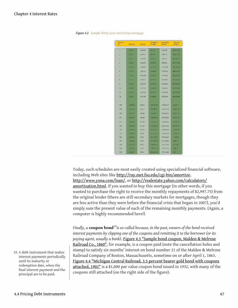
Figure 4.2 Sample thirty-year amortizing mortgage
Today, such schedules are most easily created using specialized financial software,including Web sites like http://ray.met.fsu.edu/cgi-bin/amortize,http://www.yona.com/loan/, or http://realestate.yahoo.com/calculators/amortization.html. If you wanted to buy this mortgage (in other words, if youwanted to purchase the right to receive the monthly repayments of $2,997.75) fromthe original lender (there are still secondary markets for mortgages, though theyare less active than they were before the financial crisis that began in 2007), you’dsimply sum the present value of each of the remaining monthly payments. (Again, acomputer is highly recommended here!)
Finally, a coupon bond19is so-called because, in the past, owners of the bond receivedinterest payments by clipping one of the coupons and remitting it to the borrower (or itspaying agent, usually a bank). Figure 4.3 "Sample bond coupon, Malden & MelroseRailroad Co., 1860", for example, is a coupon paid (note the cancellation holes andstamp) to satisfy six months’ interest on bond number 21 of the Malden & MelroseRailroad Company of Boston, Massachusetts, sometime on or after April 1, 1863.Figure 4.4 "Michigan Central Railroad, 3.5 percent bearer gold bond with couponsattached, 1902" is a $1,000 par value coupon bond issued in 1932, with many of thecoupons still attached (on the right side of the figure).
19. A debt instrument that makesinterest payments periodicallyuntil its maturity orredemption date, when thefinal interest payment and theprincipal are to be paid.
Chapter 4 Interest Rates
4.4 Pricing Debt Instruments 67

Figure 4.3 Sample bondcoupon, Malden & MelroseRailroad Co., 1860
Courtesy of CelebrateBoston.com
Figure 4.4 Michigan CentralRailroad, 3.5 percent bearergold bond with couponsattached, 1902
Museum of American Finance
Even if it no longer uses a physical coupon like thoseillustrated in Figure 4.3 "Sample bond coupon, Malden &Melrose Railroad Co., 1860" and Figure 4.4 "MichiganCentral Railroad, 3.5 percent bearer gold bond withcoupons attached, 1902", a coupon bond makes one ormore interest payments periodically (for example,monthly, quarterly, semiannually, annually, etc.) untilits maturity or redemption date, when the final interestpayment and all of the principal are paid. The sum of thepresent values of each future payment will give you the price.So we can calculate the price today of a $10,000 face orpar value coupon bond that pays 5 percent interestannually until its face value is redeemed (its principal isrepaid) in exactly five years if the market rate ofinterest is 6 percent, 4 percent, or any other percent forthat matter, simply by summing the present value ofeach payment:
PV1 = $500/(1.06) = $471.70 (This is the interest payment
after the first year. The $500 is the coupon20 or interestpayment, which is calculated by multiplying the bond’sface value, in this case, $10,000, by the bond’scontractual rate of interest or “coupon rate,” in thiscase, 5 percent. $10,000 × .05 = $500.)
That adds up to $9,578.77. If you are wondering why the bond is worth less than itsface value, the key is the difference between the contractual interest or coupon rateit pays, 5 percent, and the market rate of interest, 6 percent. Because the bond pays ata rate lower than the going market, people are not willing to pay as much for it, so its pricesinks below par. By the same reasoning, people should be willing to pay more than
PV2 = $500/(1.06)2 = $445.00 (If this doesn’t look familiar, you didn’t do Exercise 1 enough!)
PV3 = $500/(1.06)3 = $419.81
PV4 = $500/(1.06)4 = $396.05
PV5 = $10,500/(1.06)5 = $7,846.21
($10,500 is the final interest payment of $500 plus the repayment of the bond’s face value of $10,000.)
20. The interest rate promised tothe owner of a coupon bond.
Chapter 4 Interest Rates
4.4 Pricing Debt Instruments 68
the face value for this bond if interest rates sink below its coupon rate of 5 percent.Indeed, when the market rate of interest is 4 percent, its price is $10,445.18 (give ortake a few pennies, depending on rounding):
If the market interest rate is exactly equal to the coupon rate, the bond will sell atits par value, in this case, $10,000.00. Check it out:
Calculating the price of a bond that makes quarterly payments over thirty years canbecome quite tedious because, by the method shown above, that would entailcalculating the PV of 120 (30 years times 4 payments a year) payments. Until not toolong ago, people used special bond tables to help them make the calculations morequickly. Today, to speed things up and depending on their needs, most people use financialcalculators, specialized financial software, and canned spreadsheet functions like Excel’sPRICEDISC or PRICEMAT, custom spreadsheet formulas, or Web-based calculators likehttp://www.calculatorweb.com/calculators/bondcalc.shtml orhttp://www.investinginbonds.com/calcs/tipscalculator/TipsCalcForm.aspx. It’stime once again to get a little practice. Don’t worry; these are easy enough to workout on your own.
PV1 = $500/(1.04) = $480.77
PV2 = $500/(1.04)2 = $462.28
PV3 = $500/(1.04)3 = $444.50
PV4 = $500/(1.04)4 = $427.40
PV5 = $10,500/(1.04)5 = $8,630.23
PV1 = $500/(1.05) = $476.1905
PV2 = $500/(1.05)2 = $453.5147
PV3 = $500/(1.05)3 = $431.9188
PV4 = $500/(1.05)4 = $411.3512
PV5 = $10,500/(1.05)5 = $8,227.0247
Chapter 4 Interest Rates
4.4 Pricing Debt Instruments 69
EXERCISES
Assume no default risks or transaction costs.
1. What is the price of a 10 percent coupon bond, payable annually, with a$100 face value that matures in 3 years if interest rates are 7 percent?
2. If interest rates were 4 percent, how much would you give today for aloan with a $100,000 balloon principal payment due in a year and thatwill pay $16,000 in interest at the end of each quarter, including thefinal quarter when the principal falls due?
3. What is the value today of a share of stock that you think will be worth$50 in a year and that throws off $1 in dividends each quarter until then,assuming the market interest rate is 10 percent?
4. What is the value today of a share of stock that you think will be worth$50 in a year and that throws off $1 in dividends each quarter until thenif the market interest rate is 1 percent?
KEY TAKEAWAYS
• Debt instruments—like discount bonds, simple loans, fixed paymentloans, and coupon bonds—are contracts that promise payment in thefuture.
• They are priced by calculating the sum of the present value of thepromised payments.
Chapter 4 Interest Rates
4.4 Pricing Debt Instruments 70
4.5 What’s the Yield on That?
LEARNING OBJECTIVE
1. What is yield to maturity and for what types of financial instruments isthe yield to maturity relatively easy to calculate?
Thus far, we have assumed or been given a market interest rate and then calculatedthe price (PV) of the instrument. Or, given the PV and an interest rate, we’vecalculated the FV. Sometimes it is useful to do the opposite, to calculate the interest rate or,yield to maturity, if given the PV and FV. Say that you know that someone paid $750 fora zero coupon bond with a face value of $1,000 that will mature in exactly a yearand you want to know what interest rate he or she paid. You know that PV = FV/(1 +i). Solving for i:
You can check your work by reversing the problem—that is, asking how much you’dpay today for $1,000 in a year if interest was at 33.33 percent: PV = 1000/(1.3333333)= $750. Voilà!
Multiply each side of the equation by (1 + i) : (1 + i) × PV = FV
Multiply the terms on the left side of the equation: PV + PVi = FV
Subtract PV from each side of the equation: PVi = FV − PV
Divide each side of the equation by PV : i = (FV − PV)/PV
So in this case i = (1000 − 750)/750 = 250/750 = .3333, or 33.33 percent.
Chapter 4 Interest Rates
71
Stop and Think Box
Suppose you have $1,000 to invest for a year and two ways of investing it (eachequal in terms of risk and liquidity): a discount bond due in one year with a facevalue of $1,000 for $912 or a bank account at 6.35 percent compoundedannually. Which should you take?
Choose the bond, which will yield 9.65 percent: (1000 − 912)/912 = .0965. Tomaximize your haul, invest the $88 left over from the purchase of the bond inthe bank account.
Calculating the yield to maturity for a perpetual debt, one with no maturity or repaymentdate, like a Consol21, ground rent, or perpetual interest-only mortgage, is also quite easy.The price or PV of a perpetuity is equal to the yearly payment divided by the goingrate of interest:
So a $1,000 ground rent that pays $50 a year (a 5 percent coupon rate) would beworth $1,000 if interest rates were 5 percent, less if rates are higher, more if lower:
Calculating the yield to maturity of a perpetuity, if given the PV and FV, is easilydone by taking the equation and solving for i:
So the yield to maturity of a ground rent that pays $60 per year and that currentlysells for $600 would be 10 percent: i = 60/600 = .10 = 10%.
PV = FV/i (decimalized)
PV = 50/.05 = $1,000
PV = 50/.10 = $500
PV = 50/.01 = $5,000
PV = FV/i
Multiply each side by i : PVi = FV
Divided by PV : i = FV/PV
21. A type of perpetual bond issuedby the British government.
Chapter 4 Interest Rates
4.5 What’s the Yield on That? 72
Stop and Think Box
A ground rent contract consummated in Philadelphia, Pennsylvania, in 1756 isstill being paid today. Someone recently paid $455 for the $23.17 annualpayment. What is the ground rent’s yield to maturity? If the interest rate risesto 10 percent, how much will the ground rent be worth? What if interest falls to2 percent?
i = C/P so i = 23.17/455 = 0.05092 = 5.09%; PV = 23.17/.1 = $231.70; PV = 23.17/.02= $1,158.50.
Calculating yield to maturity for coupon bonds and fixed-payment loans, however,is mathematically nasty business without a computer or bond table. In the past,people used to estimate the yield to maturity on such instruments by pretendingthey were perpetuities or engaging in trial-and-error interpolation. In the firstmethod, you use the easy perpetuity equation above (i = FV/PV) to get a quickestimate called the current yield22. Unfortunately, current yield can be wide of themark, especially for bonds with maturities less than twenty years and bonds whose pricesare far from their par value.Current yield is simply the yield to maturity of aperpetuity, so the more like a perpetuity a bond is, the better the current yield willapproximate its yield to maturity. The shorter the maturity of a bond, the less like aConsol it is, so the less accurate the current yield formula will be. Similarly, thecurrent yield works better the closer a bond’s price is to par because yield tomaturity equals the coupon rate when the bond is at par. As the price deviatesfurther from par, the less well the current yield can approximate the yield tomaturity. In the second method, one backs into the yield to maturity by makingsuccessive guesses about i and plugging them into the PV formula. Not fun, butyou’ll eventually get there. Most people today therefore use a financial calculator,spreadsheet, or Web-based utility rather than such erroneous (current yield) orlaborious (interpolation) processes. You should be able to calculate the yield tomaturity of one-year discount bonds or perpetuities by hand, or at worst with theaid of simple (nonfinancial) calculator. Here is a little practice.
22. A quick (i = FV/PV) but flawedmethod for calculating interestrates of nonperpetual debt.
Chapter 4 Interest Rates
4.5 What’s the Yield on That? 73
EXERCISES
1. A $100 bond payable in a year sells for $97.56. What is the yield tomaturity?
2. Sam promises to pay Joe $1,904 in a year if Joe gives him $1,498 today.What interest rate is Sam paying and what interest rate Joe is earning?
3. Every year, the U.S. government pays a certain Indian tribe $10,000 and,by terms of its treaty with that tribe, must do so forever. Mr. Trumpoffered to purchase the right to receive that stream for a one-timepayment of $143,500. What yield to maturity did Trump offer theIndians?
4. What is the yield to maturity of a British Consol paying £400 per yearthat sold for £27,653?
KEY TAKEAWAYS
• Yield to maturity is the most economically accurate way of measuringnominal interest rates.
• It is easily calculated for one-year discount bonds i = (FV–PV)/PV andperpetuities i = C/PV where C is the coupon or annual payment.
Chapter 4 Interest Rates
4.5 What’s the Yield on That? 74
4.6 Calculating Returns
LEARNING OBJECTIVE
1. What is the rate of return and how does it differ from yield to maturity?
This is not all you need to know about bonds if you were to become a bond trader because thebond market, which in the United States is over 200 years old, has some odd conventions thatdo not make much economic sense. Most students will not become professional bondtraders, so in the interest of sanity, yours and ours, we will not delve into theintricacies here. (If you do become a bond trader, you will quickly and easily pick upon the conventions anyway.) Our goal here is to understand the basics of PV, FV,yield to maturity (YTM), and, finally, rate of return23. Students sometimes conflatethe last two concepts. The yield to maturity is merely a measure of the interest rate. Therate of return is more a measure of how lucrative an investment is because it accounts forchanges in the price of the bond (or other asset, financial or otherwise). More formally,
where:
R = return from holding the asset for some time period, t0 to t1
Pt0 = the price at time t0 (this can also be thought of as the purchase price)
Pt1 = the price at time t1 (this can also be thought of as the sale or going market
price)
C = coupon (or other) payment
So imagine you purchased a 5 percent coupon bond with a $100 face value thatmatures in three years when the interest rate is 5 percent. As we learned above, themarket price of such a bond would equal its face value, or $100. We also learned thatbond prices and interest rates are inversely related. As the market interest rateincreases, the PV of the bond’s future payments decreases and the bond becomesless valuable. As the rate decreases, the PV of future payments increases and thebond becomes more valuable. If the interest rate increased (decreased) to 6 (4)
R = (C + Pt1 − Pt0)/Pt0
23. A measure of the profitabilityof an investment that takesinto account changes in thevalue of the bond or otherasset.
Chapter 4 Interest Rates
75
percent, the value of the bond would decrease (increase), so the returns you earnedon the bond would not equal the yield to maturity. For example, suppose youpurchased the bond for $100 but its price a year hence stood at $103 becauseinterest rates decreased a little. Your return would be R = (5 + 3)/100 = .08, or 8%.But if in the next year, interest rates soared, driving the market price of the bonddown to $65, your return (from purchase) would be R = (10 − 35)/100 = −.25 ornegative 25%. Yes, negative. It is quite possible to lose wealth by investing in bonds orother fixed-rate financial instruments, even if there is no default (i.e., even if paymentsare punctually made as promised).
Stop and Think Box
As part of its effort to repay the large debts it accrued during the RevolutionaryWar, the U.S. federal government in the early 1790s issued three types of bonds:a coupon bond that paid 6 percent per year, a coupon bond that paid 3 percentper year, and a zero coupon bond that became a 6 percent coupon bond in 1801.For most of the 1790s and early 1800s, the price of the 6 percent bonds hoveredaround par. Given that information, what was the yield to maturity ongovernment debt in that period? What, in general terms, were the prices of the3 percent and zero coupon bonds?
The yield to maturity was about 6 percent because the 6 percent coupon bondstraded at around par. The price of the 3 percent coupon bonds must have beenwell below par because who would pay $100 to get $3 a year when she could pay$100 and get $6 a year? Finally, the zeroes must have appreciated toward theprice of the 6 percent coupon bonds as the conversion date neared.
Note that the loss is not, repeat not, predicated on actually selling the bond. One way tothink about this is that the rate of return formula merely calculates the return if thebond were to be sold. Another way to think about it is to realize that whether thebond is sold or not, its owner is still poorer by the amount of the loss because thevalue of his assets, and hence his net worth, has shrunk by that amount. The risk ofsuch loss is known as interest rate risk24 to distinguish it from other types of risks,like default risk25 (the risk of nonpayment). Interest rate risk is higher the longerthe maturity of a bond because more FVs are affected by increasing the interestrate, and the most distant ones are the most highly affected. Check this out: The PVof $1,000 in 10 years at 5% compounded annually is 1,000/(1.05)10 = $613.91. At 10%it is 1,000/(1.10)10 = $385.54, a loss of 37.2%. The PV of $1,000 in 30 years at 5% and10% is 1,000/(1.05)30 = $231.38 and 1,000/(1.10)30 = $57.31, respectively, a loss of
24. The risk that the market priceof a bond or other debtinstrument will decrease dueto increases in the interestrate.
25. The risk that a bond or otherdebt instrument will not makethe promised payments.
Chapter 4 Interest Rates
4.6 Calculating Returns 76
75.23 percent. Duration is a technical measure of interest rate risk that we will notinvestigate here, where the main point is merely that rising interest rates hurt bondprices (and hence bondholders); falling interest rates help bond prices.
KEY TAKEAWAYS
• The rate of return accounts for changes in the market price of a bond orother asset while the yield to maturity does not.
• Yield to maturity (YTM) is almost always positive but returns are oftennegative due to interest rate risk, the risk that interest rates will rise,depressing bond prices.
• When the market interest rate increases, bond prices decrease becausethe opportunity cost of lending money has increased, making bonds lessattractive investments unless their price falls.
• Algebraically, PV = FV/(1 + i)n. The interest rate is in the denominator,so as i gets bigger, PV must get smaller.
• Bonds with longer periods to maturity have more volatile prices, ceterisparibus, because the PV of their distant FV shrinks more, to very smallsums.
Chapter 4 Interest Rates
4.6 Calculating Returns 77
4.7 Inflation and Interest Rates
LEARNING OBJECTIVE
1. What is the difference between real and nominal interest rates and whyis the distinction important?
You might well ask at this point, What factors change interest rates? One big factoris inflation. As the price level rises, so too do interest rates, or at least whateconomists call nominal interest rates, the type of rates we’ve discussed so far. Ifnominal rates do not increase (and they often don’t, or can’t), lenders might receive morenominal dollars than they lent but actually get back less purchasing power. Imagine, forexample, that you lent $100 for one year at 6 percent interest when a loaf of bread,pack of chewing gum, and two-liter bottle of Mountain Dew each cost $1. At the endof the simple loan, you would get back $100 × 1.06 = $106 and be able to enjoy anextra $6 of goods, say, two loaves of bread, two packs of gum, and two bottles of thecaffeine and sugar rush known as Doin’ the Dew. But what if prices doubled overthat year? Instead of some combination of 106 goodies, you’d be able to buy onlyfifty-three. Your nominal return would be positive, but your real return, what youcould actually buy with the $106, would be steeply negative.
A simple equation, the Fisher Equation, named after Irving Fisher, the early twentieth-century U.S. economist who articulated it,To be frank, Benjamin Franklin and othercolonists in eighteenth-century America understood it well.helps us to understand therelationship between inflation and interest rates more precisely:
where
ir = the real interest rate
i = the nominal interest rate (the type of interest rate the first part of this chapterdiscussed exclusively)
1= inflation (or expected inflation)
i = ir + π or, rearranging the terms, ir = i − π or, again rearranging the terms, π = i − ir
Chapter 4 Interest Rates
78
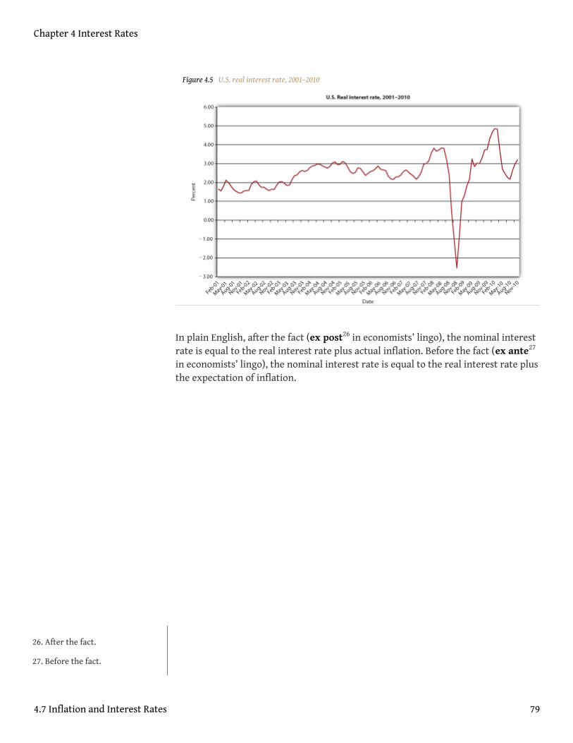
Figure 4.5 U.S. real interest rate, 2001–2010
In plain English, after the fact (ex post26 in economists’ lingo), the nominal interestrate is equal to the real interest rate plus actual inflation. Before the fact (ex ante27
in economists’ lingo), the nominal interest rate is equal to the real interest rate plusthe expectation of inflation.
26. After the fact.
27. Before the fact.
Chapter 4 Interest Rates
4.7 Inflation and Interest Rates 79
Stop and Think Box
In early 2007, a man had a wallet returned that he had lost over sixty yearsearlier in France, during World War II.ABC News video, “Wallet Returned, 60Years Later, A World War II Veteran gets his wallet returned to him sixty yearslater” (1/9/2007). In addition to his original Social Security card and a pictureof his parents, the man received an unspecified sum of cash. Was losing thewallet a good investment? Why or why not?
No, because the risk that it would never be returned was very high. Plus, thedollar lost a significant amount of its purchasing power over the period due toinflation and the money earned no interest. At just 3 percent compoundedannually, $100 would have grown to 100 × (1.03)60 = $589.16 after 60 years. At 6percent, $100 would have grown to 100 × (1.06)60 = $3,298.77.
Traditionally, inflation expectations were unobservable so real rates wereknown only ex post. However, relatively new and special types of bondsindexed to inflation, called Treasury Inflation Protection Securities (TIPS),provide real interest rate information, allowing market participants to observeex ante inflation expectations. For example, if the yield to maturity on aregular, nonindexed ten-year Treasury bond is 5 percent, and the yield on theten-year TIPS is 2 percent, the inflation expectation, via the Fisher Equation π =i − ir, is 5 −2 = 3 percent. Figure 4.5 "U.S. real interest rate, 2001–2010" shows
how inflation expectations have waxed and waned since the introduction ofTIPS in 1997.
KEY TAKEAWAYS
• The difference between the real and the nominal interest rate is literallyinflation or inflation expectations.
• According to the Fisher Equation, nominal interest equals real interestplus inflation (or inflation expectations), or real interest equals nominalinterest minus inflation (expectations).
• If actual inflation exceeds inflation expectations, real ex post (inflation-adjusted, after the fact) returns on bonds can be negative.
Chapter 4 Interest Rates
4.7 Inflation and Interest Rates 80
4.8 Suggested Reading
Fisher, Irving. The Purchasing Power of Money: Its Determination and Relation to CreditInterest and Crises. New York: Cosimo Classics, 2006.
Strumeyer, Gary. Investing in Fixed Income Securities: Understanding the Bond Market.Hoboken, NJ: John Wiley and Sons, 2005.
Wild, Russell. Bond Investing for Dummies. Hoboken, NJ: John Wiley and Sons, 2007.
Chapter 4 Interest Rates
81
Chapter 5
The Economics of Interest-Rate Fluctuations
CHAPTER OBJECTIVES
By the end of this chapter, students should be able to
1. Describe, at the first level of analysis, the factors that cause changes inthe interest rate.
2. List and explain four major factors that determine the quantitydemanded of an asset.
3. List and explain three major factors that cause shifts in the bond supplycurve.
4. Explain why the Fisher Equation holds; that is, explain why theexpectation of higher inflation leads to a higher nominal interest rate.
5. Predict, in a general way, what will happen to the interest rate during aneconomic expansion or contraction and explain why.
6. Discuss how changes in the money supply may affect interest rates.
82
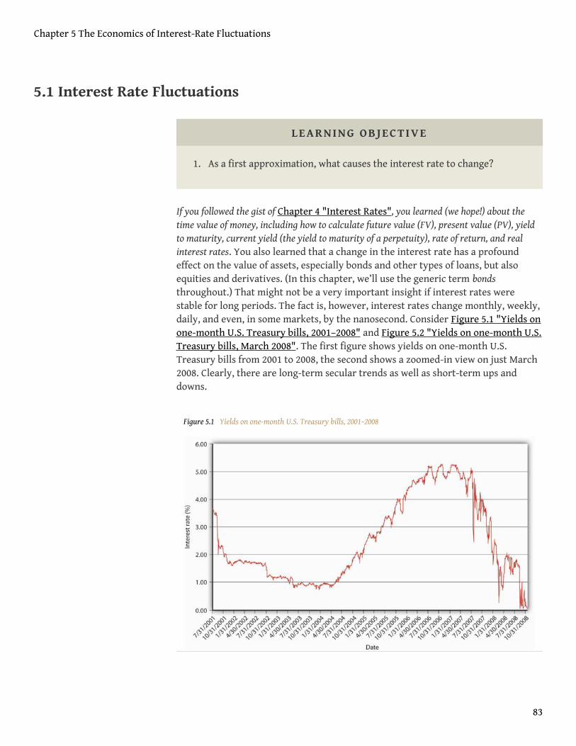
5.1 Interest Rate Fluctuations
LEARNING OBJECTIVE
1. As a first approximation, what causes the interest rate to change?
If you followed the gist of Chapter 4 "Interest Rates", you learned (we hope!) about thetime value of money, including how to calculate future value (FV), present value (PV), yieldto maturity, current yield (the yield to maturity of a perpetuity), rate of return, and realinterest rates. You also learned that a change in the interest rate has a profoundeffect on the value of assets, especially bonds and other types of loans, but alsoequities and derivatives. (In this chapter, we’ll use the generic term bondsthroughout.) That might not be a very important insight if interest rates werestable for long periods. The fact is, however, interest rates change monthly, weekly,daily, and even, in some markets, by the nanosecond. Consider Figure 5.1 "Yields onone-month U.S. Treasury bills, 2001–2008" and Figure 5.2 "Yields on one-month U.S.Treasury bills, March 2008". The first figure shows yields on one-month U.S.Treasury bills from 2001 to 2008, the second shows a zoomed-in view on just March2008. Clearly, there are long-term secular trends as well as short-term ups anddowns.
Figure 5.1 Yields on one-month U.S. Treasury bills, 2001–2008
Chapter 5 The Economics of Interest-Rate Fluctuations
83
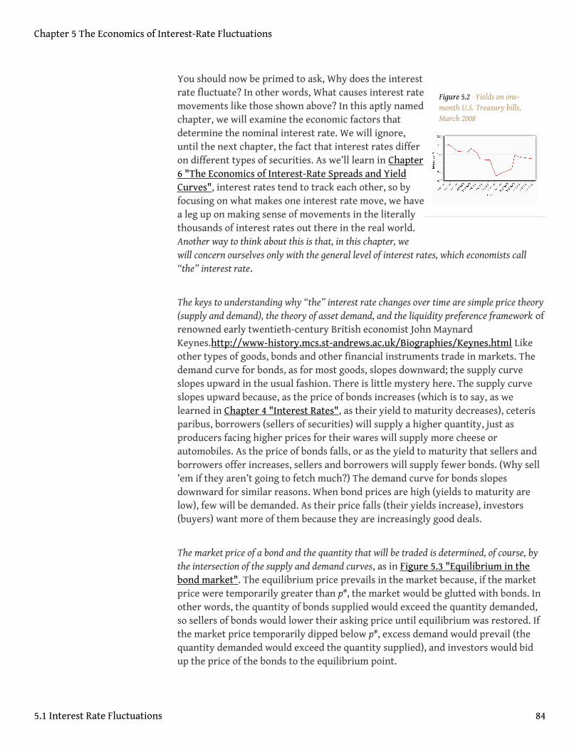
Figure 5.2 Yields on one-month U.S. Treasury bills,March 2008
You should now be primed to ask, Why does the interestrate fluctuate? In other words, What causes interest ratemovements like those shown above? In this aptly namedchapter, we will examine the economic factors thatdetermine the nominal interest rate. We will ignore,until the next chapter, the fact that interest rates differon different types of securities. As we’ll learn in Chapter6 "The Economics of Interest-Rate Spreads and YieldCurves", interest rates tend to track each other, so byfocusing on what makes one interest rate move, we havea leg up on making sense of movements in the literallythousands of interest rates out there in the real world.Another way to think about this is that, in this chapter, wewill concern ourselves only with the general level of interest rates, which economists call“the” interest rate.
The keys to understanding why “the” interest rate changes over time are simple price theory(supply and demand), the theory of asset demand, and the liquidity preference framework ofrenowned early twentieth-century British economist John MaynardKeynes.http://www-history.mcs.st-andrews.ac.uk/Biographies/Keynes.html Likeother types of goods, bonds and other financial instruments trade in markets. Thedemand curve for bonds, as for most goods, slopes downward; the supply curveslopes upward in the usual fashion. There is little mystery here. The supply curveslopes upward because, as the price of bonds increases (which is to say, as welearned in Chapter 4 "Interest Rates", as their yield to maturity decreases), ceterisparibus, borrowers (sellers of securities) will supply a higher quantity, just asproducers facing higher prices for their wares will supply more cheese orautomobiles. As the price of bonds falls, or as the yield to maturity that sellers andborrowers offer increases, sellers and borrowers will supply fewer bonds. (Why sell’em if they aren’t going to fetch much?) The demand curve for bonds slopesdownward for similar reasons. When bond prices are high (yields to maturity arelow), few will be demanded. As their price falls (their yields increase), investors(buyers) want more of them because they are increasingly good deals.
The market price of a bond and the quantity that will be traded is determined, of course, bythe intersection of the supply and demand curves, as in Figure 5.3 "Equilibrium in thebond market". The equilibrium price prevails in the market because, if the marketprice were temporarily greater than p*, the market would be glutted with bonds. Inother words, the quantity of bonds supplied would exceed the quantity demanded,so sellers of bonds would lower their asking price until equilibrium was restored. Ifthe market price temporarily dipped below p*, excess demand would prevail (thequantity demanded would exceed the quantity supplied), and investors would bidup the price of the bonds to the equilibrium point.
Chapter 5 The Economics of Interest-Rate Fluctuations
5.1 Interest Rate Fluctuations 84
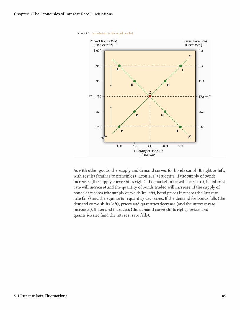
Figure 5.3 Equilibrium in the bond market
As with other goods, the supply and demand curves for bonds can shift right or left,with results familiar to principles (“Econ 101”) students. If the supply of bondsincreases (the supply curve shifts right), the market price will decrease (the interestrate will increase) and the quantity of bonds traded will increase. If the supply ofbonds decreases (the supply curve shifts left), bond prices increase (the interestrate falls) and the equilibrium quantity decreases. If the demand for bonds falls (thedemand curve shifts left), prices and quantities decrease (and the interest rateincreases). If demand increases (the demand curve shifts right), prices andquantities rise (and the interest rate falls).
Chapter 5 The Economics of Interest-Rate Fluctuations
5.1 Interest Rate Fluctuations 85
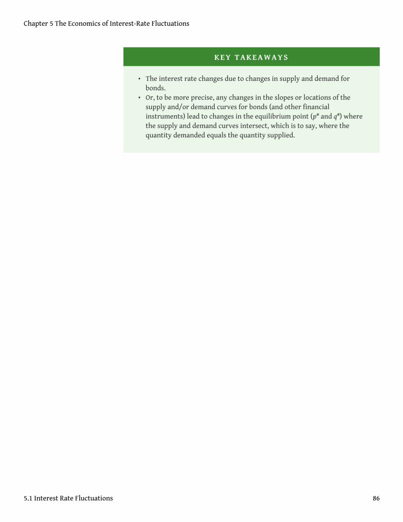
KEY TAKEAWAYS
• The interest rate changes due to changes in supply and demand forbonds.
• Or, to be more precise, any changes in the slopes or locations of thesupply and/or demand curves for bonds (and other financialinstruments) lead to changes in the equilibrium point (p* and q*) wherethe supply and demand curves intersect, which is to say, where thequantity demanded equals the quantity supplied.
Chapter 5 The Economics of Interest-Rate Fluctuations
5.1 Interest Rate Fluctuations 86
5.2 Shifts in Supply and Demand for Bonds
LEARNING OBJECTIVE
1. What causes the supply and demand for bonds to shift?
Shifting supply and demand curves around can be fun, but figuring out why the curves shiftis the interesting part. (Determining the shape and slope of the curves is interestingtoo, but these details will not detain us here.) Movements along the curve, or whythe supply curve slopes upward and the demand curve downward, were easyenough to grasp. Determining why the whole curve moves, why investors arewilling to buy more (or fewer) bonds, or why borrowers are willing to sell more (orfewer) bonds at a given price is a bit more involved. Let’s tackle demand first, thenwe will move on to supply.
Wealth determines the overall demand for assets. An asset (something owned) is anystore of value, including financial assets like money, loans (for the lender), bonds,equities (stocks), and a potpourri of derivativeshttp://www.margrabe.com/Dictionary/DictionaryAC.html#sectA and nonfinancial assets like real estate (land,buildings), precious metals (gold, silver, platinum), gems (diamonds, rubies,emeralds), hydrocarbons (oil, natural gas) and (to a greater or lesser extent,depending on their qualities) all other physical goods (as opposed to bads, likepollution, or freebies, like air). As wealth increases, so too does the quantitydemanded of all types of assets, though to different degrees. The reasoning here isalmost circular: if it is to be maintained, wealth must be invested in some asset, insome store of value. In which type of asset to invest new wealth is the difficultdecision. When determining which assets to hold, most economic entities (people,firms, governments) care about many factors, but for most investors most of thetime, three variables—expected relative return, risk, and liquidity—are paramount.(We briefly discussed these concepts, you may recall, in Chapter 2 "The FinancialSystem".)
Expected relative return is the ex ante (before the fact) belief that the return on oneasset will be higher than the returns of other comparable (in terms of risk andliquidity) assets. Return is a good thing, of course, so as expected relative return increases,the quantity demanded of an asset also increases. That can happen because the expectedreturn on the asset itself increases, because the expected return on comparablesdecreases, or because of a combination thereof. Clearly, two major factors discussedin Chapter 4 "Interest Rates" will affect return expectations and hence the demand
Chapter 5 The Economics of Interest-Rate Fluctuations
87

for certain financial assets, like bonds: expected interest rates and, via the FisherEquation, expected inflation. If the interest rate is expected to increase for anyreason (including, but not limited to, expected increases in inflation), bond pricesare expected to fall, so the quantity demanded will decrease. Conversely, if theinterest rate is thought to decrease for any reason (including, but not limited to, theexpected taming of inflation), bond prices are expected to rise, so the quantitydemanded will increase.
Overall, though, calculating relative expected returns is sticky business that is bestaddressed in more specialized financial books and courses. If you want anintroduction, investigate the capital asset pricing model(CAPM)http://www.valuebasedmanagement.net/methods_capm.html;http://www.moneychimp.com/articles/valuation/capm.htmand the arbitrage pricing theory (APT).http://moneyterms.co.uk/apt/ As welearned in Chapter 4 "Interest Rates", calculating return is not terribly difficult andneither is comparing returns among a variety of assets. What’s tricky is forecastingfuture returns and making sure that assets are comparable by controlling for risk,among other things. Risk is the uncertainty of an asset’s returns. It comes in a variety offlavors, all of them unsavory, so as it increases, the quantity demanded of an asset decreases,ceteris paribus. In Chapter 4 "Interest Rates", we encountered two types of risk:default risk (aka credit risk), the chance that a financial contract will not behonored, and interest rate risk, the chance that the interest rate will rise and hencedecrease a bond or loan’s price. An offsetting risk is called reinvestment risk, whichbites when the interest rate decreases because coupon or other interest paymentshave to be reinvested at a lower yield to maturity. To be willing to take on more risk,whatever its flavor, rational investors must expect a higher relative return. Investors whorequire a much higher return for assuming a little bit of risk are called risk-averse.Those who will take on much risk for a little higher return are called risk-loving,risk-seekers, or risk-tolerant. (Investors who take on more risk withoutcompensation are neither risk-averse nor risk-tolerant, but rather irrational in thesense discussed in Chapter 7 "Rational Expectations, Efficient Markets, and theValuation of Corporate Equities".) Risks can be idiosyncratic; that is, they can bepertinent to a particular company, sectoral (pertinent to an entire industry, liketrucking or restaurants), or systemic (economy-wide). Liquidity risk occurs when anasset cannot be sold as quickly or cheaply as expected, be it for idiosyncratic,sectoral, or systemic reasons. This, too, is a serious risk because liquidity, or (to be moreprecise) liquidity relative to other assets, is the third major determinant of asset demand.Because investors often need to change their investment portfolio1 or dis-save(spend some of their wealth on consumption), liquidity, the ability to sell an assetquickly and cheaply, is a good thing. The more liquid an asset is, therefore, thehigher the quantity demanded, all else being equal.
1. The set of financial and otherinvestments or assets held byan economic entity.
Chapter 5 The Economics of Interest-Rate Fluctuations
5.2 Shifts in Supply and Demand for Bonds 88
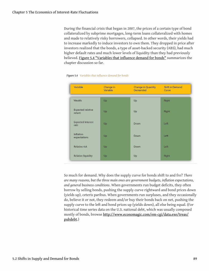
During the financial crisis that began in 2007, the prices of a certain type of bondcollateralized by subprime mortgages, long-term loans collateralized with homesand made to relatively risky borrowers, collapsed. In other words, their yields hadto increase markedly to induce investors to own them. They dropped in price afterinvestors realized that the bonds, a type of asset-backed security (ABS), had muchhigher default rates and much lower levels of liquidity than they had previouslybelieved. Figure 5.4 "Variables that influence demand for bonds" summarizes thechapter discussion so far.
Figure 5.4 Variables that influence demand for bonds
So much for demand. Why does the supply curve for bonds shift to and fro? Thereare many reasons, but the three main ones are government budgets, inflation expectations,and general business conditions. When governments run budget deficits, they oftenborrow by selling bonds, pushing the supply curve rightward and bond prices down(yields up), ceteris paribus. When governments run surpluses, and they occasionallydo, believe it or not, they redeem and/or buy their bonds back on net, pushing thesupply curve to the left and bond prices up (yields down), all else being equal. (Forhistorical time series data on the U.S. national debt, which was usually composedmostly of bonds, browse http://www.economagic.com/em-cgi/data.exe/treas/pubdebt.)
Chapter 5 The Economics of Interest-Rate Fluctuations
5.2 Shifts in Supply and Demand for Bonds 89
Stop and Think Box
You are a copyeditor for Barron’s. What, if anything, appears wrong in thefollowing sentence? How do you know?
“Recent increases in the profitability of investments, inflation expectations,and government surpluses will surely lead to increased bond supplies in thenear future.”
Government deficits, not surpluses, lead to increased bond supplies.
The expectation of higher inflation, other factors held constant, will causeborrowers to issue more bonds, driving the supply curve rightward, and bondprices down (and yields up). The Fisher Equation, ir = i – πe, explains this nicely. If
the inflation expectation term πe increases while nominal interest rate i stays thesame, the real interest rate ir must decrease. From the perspective of borrowers, the real
cost of borrowing falls, which means that borrowing becomes more attractive. So they sellbonds.
Borrowing also becomes more attractive when general business conditions become morefavorable, as when taxes and regulatory costs decrease or the economy expands. Althoughindividuals sometimes try to borrow out of financial weakness or desperation,relatively few such loans are made because they are high risk. Most economicentities borrow out of strength, to finance expansion and engage in new projectsthey believe will be profitable. So when economic prospects are good, taxes are low,and regulations are not too costly, businesses are eager to borrow, often by sellingbonds, shifting the supply curve to the right and bond prices down (yields up).Figure 5.5 "Variables that determine the supply of bonds" summarizes the chapterdiscussion so far.
Chapter 5 The Economics of Interest-Rate Fluctuations
5.2 Shifts in Supply and Demand for Bonds 90
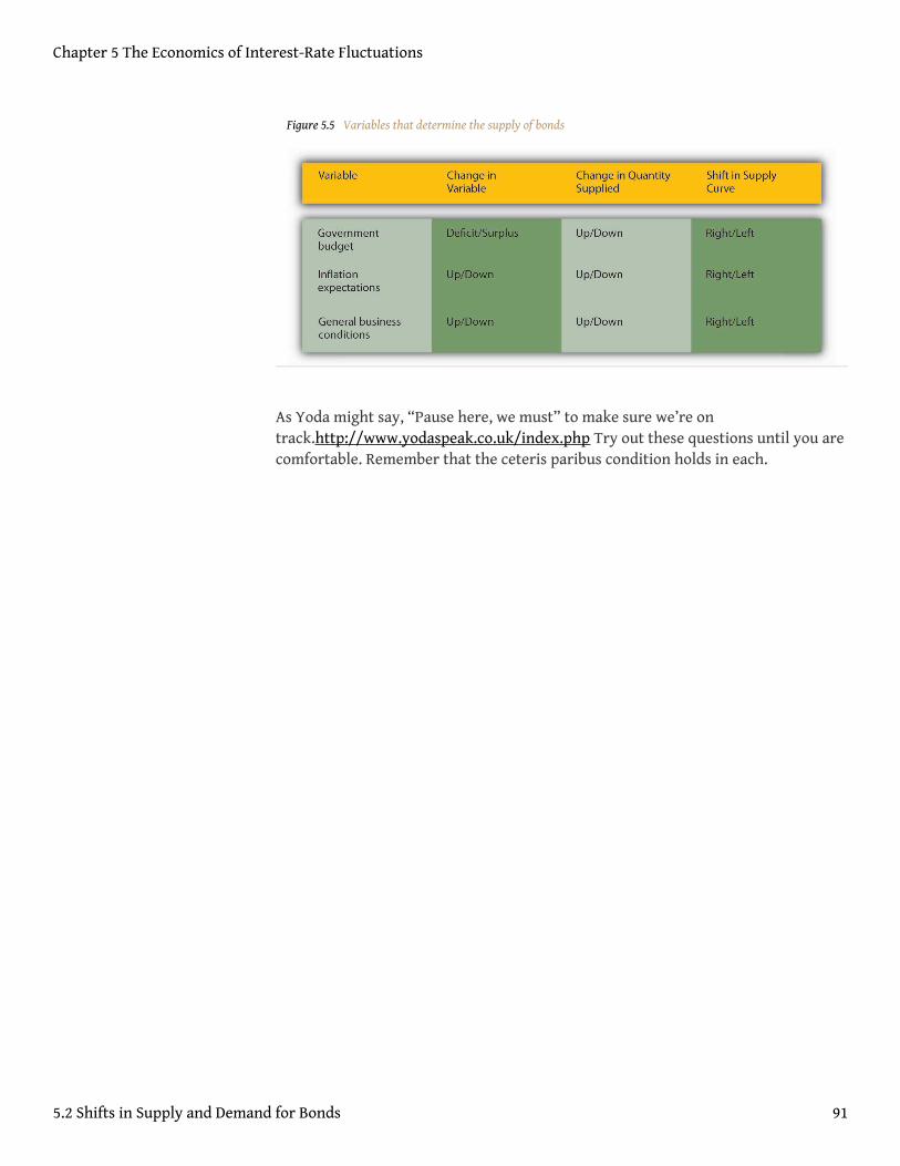
Figure 5.5 Variables that determine the supply of bonds
As Yoda might say, “Pause here, we must” to make sure we’re ontrack.http://www.yodaspeak.co.uk/index.php Try out these questions until you arecomfortable. Remember that the ceteris paribus condition holds in each.
Chapter 5 The Economics of Interest-Rate Fluctuations
5.2 Shifts in Supply and Demand for Bonds 91
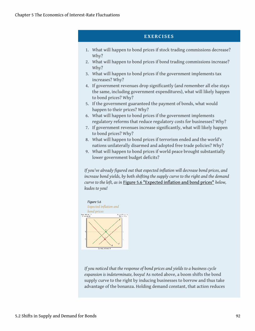
EXERCISES
1. What will happen to bond prices if stock trading commissions decrease?Why?
2. What will happen to bond prices if bond trading commissions increase?Why?
3. What will happen to bond prices if the government implements taxincreases? Why?
4. If government revenues drop significantly (and remember all else staysthe same, including government expenditures), what will likely happento bond prices? Why?
5. If the government guaranteed the payment of bonds, what wouldhappen to their prices? Why?
6. What will happen to bond prices if the government implementsregulatory reforms that reduce regulatory costs for businesses? Why?
7. If government revenues increase significantly, what will likely happento bond prices? Why?
8. What will happen to bond prices if terrorism ended and the world’snations unilaterally disarmed and adopted free trade policies? Why?
9. What will happen to bond prices if world peace brought substantiallylower government budget deficits?
If you’ve already figured out that expected inflation will decrease bond prices, andincrease bond yields, by both shifting the supply curve to the right and the demandcurve to the left, as in Figure 5.6 "Expected inflation and bond prices" below,kudos to you!
Figure 5.6Expected inflation andbond prices
If you noticed that the response of bond prices and yields to a business cycleexpansion is indeterminate, booya! As noted above, a boom shifts the bondsupply curve to the right by inducing businesses to borrow and thus takeadvantage of the bonanza. Holding demand constant, that action reduces
Chapter 5 The Economics of Interest-Rate Fluctuations
5.2 Shifts in Supply and Demand for Bonds 92
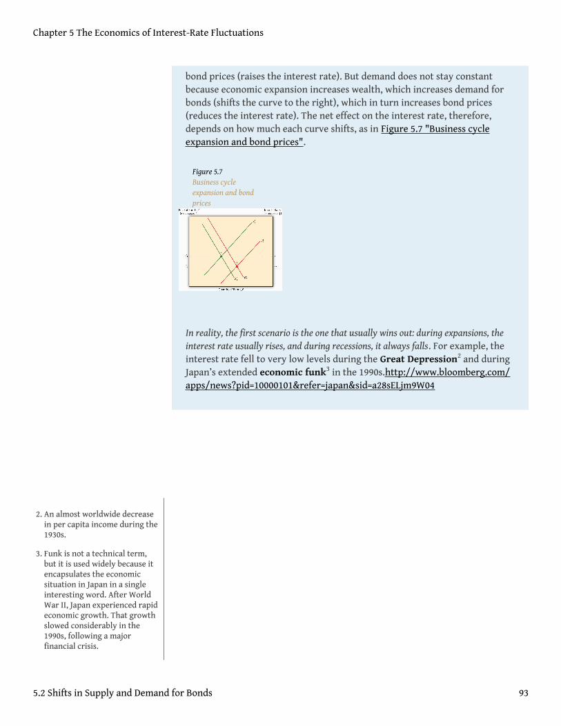
bond prices (raises the interest rate). But demand does not stay constantbecause economic expansion increases wealth, which increases demand forbonds (shifts the curve to the right), which in turn increases bond prices(reduces the interest rate). The net effect on the interest rate, therefore,depends on how much each curve shifts, as in Figure 5.7 "Business cycleexpansion and bond prices".
Figure 5.7Business cycleexpansion and bondprices
In reality, the first scenario is the one that usually wins out: during expansions, theinterest rate usually rises, and during recessions, it always falls. For example, theinterest rate fell to very low levels during the Great Depression2 and duringJapan’s extended economic funk3 in the 1990s.http://www.bloomberg.com/apps/news?pid=10000101&refer=japan&sid=a28sELjm9W04
2. An almost worldwide decreasein per capita income during the1930s.
3. Funk is not a technical term,but it is used widely because itencapsulates the economicsituation in Japan in a singleinteresting word. After WorldWar II, Japan experienced rapideconomic growth. That growthslowed considerably in the1990s, following a majorfinancial crisis.
Chapter 5 The Economics of Interest-Rate Fluctuations
5.2 Shifts in Supply and Demand for Bonds 93

KEY TAKEAWAYS
• The demand curve for bonds shifts due to changes in wealth, expectedrelative returns, risk, and liquidity.
• Wealth, returns, and liquidity are positively related to demand; risk isinversely related to demand.
• Wealth sets the general level of demand. Investors then trade off risk forreturns and liquidity.
• The supply curve for bonds shifts due to changes in governmentbudgets, inflation expectations, and general business conditions.
• Deficits cause governments to issue bonds and hence shift the bondsupply curve right; surpluses have the opposite effect.
• Expected inflation leads businesses to issue bonds because inflationreduces real borrowing costs, ceteris paribus; decreases in expectedinflation or deflation expectations have the opposite effect.
• Expectations of future general business conditions, including taxreductions, regulatory cost reduction, and increased economic growth(economic expansion or boom), induce businesses to borrow (issuebonds), while higher taxes, more costly regulations, and recessions shiftthe bond supply curve left.
• Theoretically, whether a business expansion leads to higher interestrates or not depends on the degree of the shift in the bond supply anddemand curves.
• An expansion will cause the bond supply curve to shift right, whichalone will decrease bond prices (increase the interest rate).
• But expansions also cause the demand for bonds to increase (the bonddemand curve to shift right), which has the effect of increasing bondprices (and hence lowering bond yields).
• Empirically, the bond supply curve typically shifts much further thanthe bond demand curve, so the interest rate usually rises duringexpansions and always falls during recessions.
Chapter 5 The Economics of Interest-Rate Fluctuations
5.2 Shifts in Supply and Demand for Bonds 94
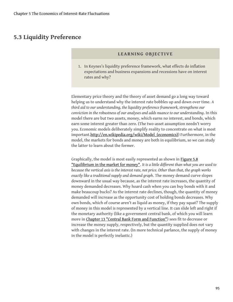
5.3 Liquidity Preference
LEARNING OBJECTIVE
1. In Keynes’s liquidity preference framework, what effects do inflationexpectations and business expansions and recessions have on interestrates and why?
Elementary price theory and the theory of asset demand go a long way towardhelping us to understand why the interest rate bobbles up and down over time. Athird aid to our understanding, the liquidity preference framework, strengthens ourconviction in the robustness of our analyses and adds nuance to our understanding. In thismodel there are but two assets, money, which earns no interest, and bonds, whichearn some interest greater than zero. (The two-asset assumption needn’t worryyou. Economic models deliberately simplify reality to concentrate on what is mostimportant.http://en.wikipedia.org/wiki/Model_(economics)) Furthermore, in themodel, the markets for bonds and money are both in equilibrium, so we can studythe latter to learn about the former.
Graphically, the model is most easily represented as shown in Figure 5.8"Equilibrium in the market for money". It is a little different than what you are used tobecause the vertical axis is the interest rate, not price. Other than that, the graph worksexactly like a traditional supply and demand graph. The money demand curve slopesdownward in the usual way because, as the interest rate increases, the quantity ofmoney demanded decreases. Why hoard cash when you can buy bonds with it andmake beaucoup bucks? As the interest rate declines, though, the quantity of moneydemanded will increase as the opportunity cost of holding bonds decreases. Whyown bonds, which of course aren’t as liquid as money, if they pay squat? The supplyof money in this model is represented by a vertical line. It can slide left and right ifthe monetary authority (like a government central bank, of which you will learnmore in Chapter 13 "Central Bank Form and Function") sees fit to decrease orincrease the money supply, respectively, but the quantity supplied does not varywith changes in the interest rate. (In more technical parlance, the supply of moneyin the model is perfectly inelastic.)
Chapter 5 The Economics of Interest-Rate Fluctuations
95
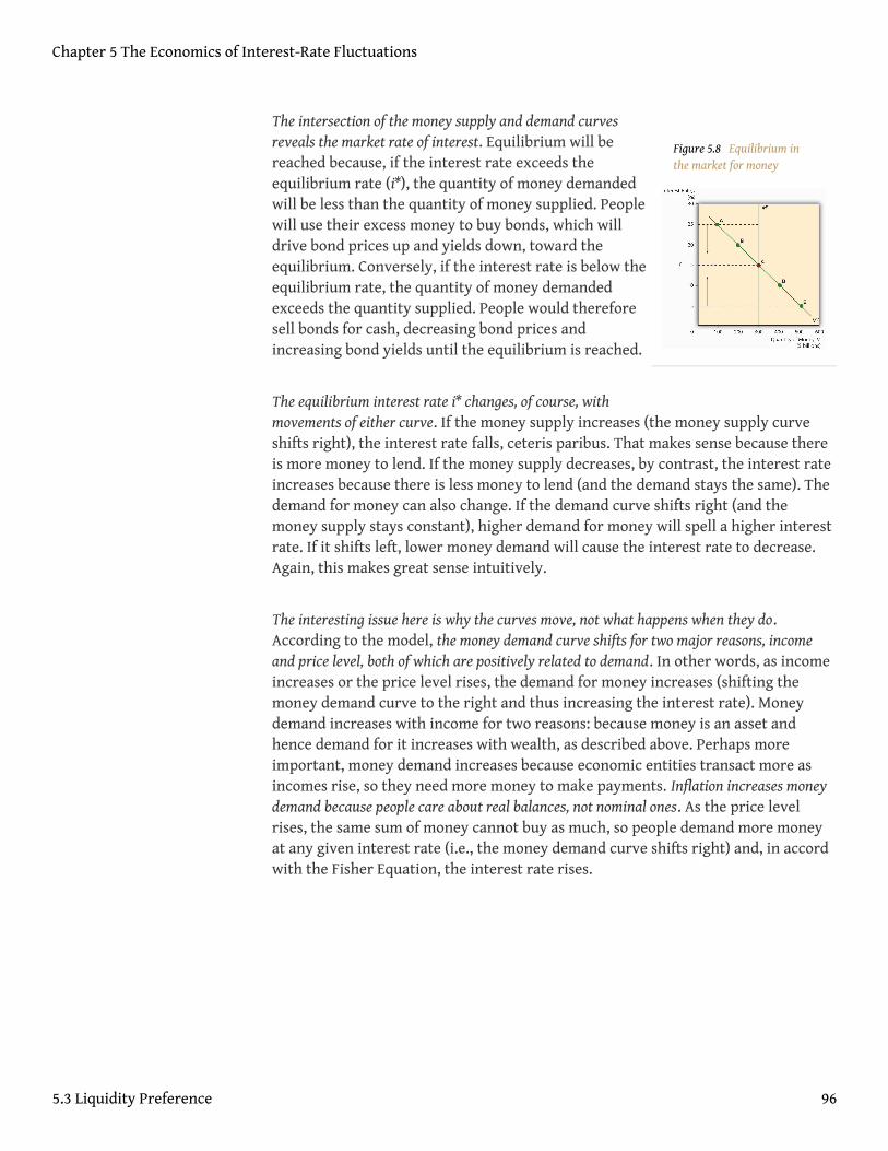
Figure 5.8 Equilibrium inthe market for money
The intersection of the money supply and demand curvesreveals the market rate of interest. Equilibrium will bereached because, if the interest rate exceeds theequilibrium rate (i*), the quantity of money demandedwill be less than the quantity of money supplied. Peoplewill use their excess money to buy bonds, which willdrive bond prices up and yields down, toward theequilibrium. Conversely, if the interest rate is below theequilibrium rate, the quantity of money demandedexceeds the quantity supplied. People would thereforesell bonds for cash, decreasing bond prices andincreasing bond yields until the equilibrium is reached.
The equilibrium interest rate i* changes, of course, withmovements of either curve. If the money supply increases (the money supply curveshifts right), the interest rate falls, ceteris paribus. That makes sense because thereis more money to lend. If the money supply decreases, by contrast, the interest rateincreases because there is less money to lend (and the demand stays the same). Thedemand for money can also change. If the demand curve shifts right (and themoney supply stays constant), higher demand for money will spell a higher interestrate. If it shifts left, lower money demand will cause the interest rate to decrease.Again, this makes great sense intuitively.
The interesting issue here is why the curves move, not what happens when they do.According to the model, the money demand curve shifts for two major reasons, incomeand price level, both of which are positively related to demand. In other words, as incomeincreases or the price level rises, the demand for money increases (shifting themoney demand curve to the right and thus increasing the interest rate). Moneydemand increases with income for two reasons: because money is an asset andhence demand for it increases with wealth, as described above. Perhaps moreimportant, money demand increases because economic entities transact more asincomes rise, so they need more money to make payments. Inflation increases moneydemand because people care about real balances, not nominal ones. As the price levelrises, the same sum of money cannot buy as much, so people demand more moneyat any given interest rate (i.e., the money demand curve shifts right) and, in accordwith the Fisher Equation, the interest rate rises.
Chapter 5 The Economics of Interest-Rate Fluctuations
5.3 Liquidity Preference 96
Stop and Think Box
You are a consultant for a company considering issuing bonds when you findthe following message in your e-mail inbox:
From: Reuters News Service
Re: “Economists Express Concern Over Inflation”
“Is inflation beginning to awaken from its long slumber? . . . Some economistsare beginning to detect signs of strain. They worry that recent inflation reportswere pushed down by unusually large price decreases in certain areas, whichbuck recent trends and are unlikely to recur. Absent those drops, the overallinflation numbers would have edged higher. . . . Other economists argue thatmany companies are just beginning to feel the bite of skyrocketing energycosts. . . . Businesses are unlikely to watch profit margins continue to shrinkwithout forcing through price increases. Other companies have locked in lowerenergy costs by skillfully using futures markets, but those options are set toexpire, leaving the businesses unprotected.”
What do you advise your clients regarding their bond issue deliberations? Why?
According to Irving Fisher, when expected inflation rises, the interest rate willrise. This well-known Fisher effect, which is confirmed by both the theory ofasset demand and Keynes’s liquidity preference framework, suggests that thecompany will have to pay a higher yield on its bonds than anticipated becausethe higher expected inflation will reduce the expected return on bonds relativeto real assets, shifting the demand curve to the left. Also, the real cost ofborrowing will decrease, causing the quantity of bonds supplied to the marketto increase and the supply curve to shift to the right. Both reduced demand andincreased supply leads to a decrease in bond prices, that is, an increase in bondyields. Or, in Keynes’s framework, the demand for money increases withinflation expectations because people want to maintain real money balances.Any way you slice it, the company is facing the prospect of paying higher yieldson its bonds in the near future.
Chapter 5 The Economics of Interest-Rate Fluctuations
5.3 Liquidity Preference 97
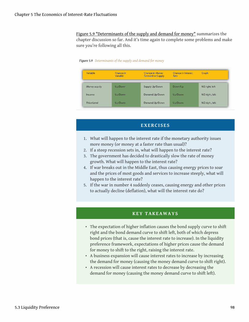
Figure 5.9 "Determinants of the supply and demand for money" summarizes thechapter discussion so far. And it’s time again to complete some problems and makesure you’re following all this.
Figure 5.9 Determinants of the supply and demand for money
EXERCISES
1. What will happen to the interest rate if the monetary authority issuesmore money (or money at a faster rate than usual)?
2. If a steep recession sets in, what will happen to the interest rate?3. The government has decided to drastically slow the rate of money
growth. What will happen to the interest rate?4. If war breaks out in the Middle East, thus causing energy prices to soar
and the prices of most goods and services to increase steeply, what willhappen to the interest rate?
5. If the war in number 4 suddenly ceases, causing energy and other pricesto actually decline (deflation), what will the interest rate do?
KEY TAKEAWAYS
• The expectation of higher inflation causes the bond supply curve to shiftright and the bond demand curve to shift left, both of which depressbond prices (that is, cause the interest rate to increase). In the liquiditypreference framework, expectations of higher prices cause the demandfor money to shift to the right, raising the interest rate.
• A business expansion will cause interest rates to increase by increasingthe demand for money (causing the money demand curve to shift right).
• A recession will cause interest rates to decrease by decreasing thedemand for money (causing the money demand curve to shift left).
Chapter 5 The Economics of Interest-Rate Fluctuations
5.3 Liquidity Preference 98
Chapter 5 The Economics of Interest-Rate Fluctuations
5.3 Liquidity Preference 99
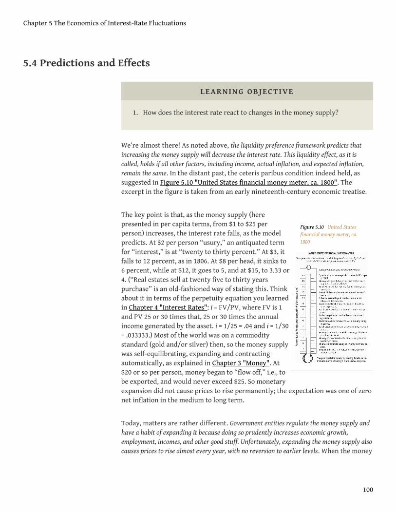
Figure 5.10 United Statesfinancial money meter, ca.1800
5.4 Predictions and Effects
LEARNING OBJECTIVE
1. How does the interest rate react to changes in the money supply?
We’re almost there! As noted above, the liquidity preference framework predicts thatincreasing the money supply will decrease the interest rate. This liquidity effect, as it iscalled, holds if all other factors, including income, actual inflation, and expected inflation,remain the same. In the distant past, the ceteris paribus condition indeed held, assuggested in Figure 5.10 "United States financial money meter, ca. 1800". Theexcerpt in the figure is taken from an early nineteenth-century economic treatise.
The key point is that, as the money supply (herepresented in per capita terms, from $1 to $25 perperson) increases, the interest rate falls, as the modelpredicts. At $2 per person “usury,” an antiquated termfor “interest,” is at “twenty to thirty percent.” At $3, itfalls to 12 percent, as in 1806. At $8 per head, it sinks to6 percent, while at $12, it goes to 5, and at $15, to 3.33 or4. (“Real estates sell at twenty five to thirty yearspurchase” is an old-fashioned way of stating this. Thinkabout it in terms of the perpetuity equation you learnedin Chapter 4 "Interest Rates": i = FV/PV, where FV is 1and PV 25 or 30 times that, 25 or 30 times the annualincome generated by the asset. i = 1/25 = .04 and i = 1/30= .033333.) Most of the world was on a commoditystandard (gold and/or silver) then, so the money supplywas self-equilibrating, expanding and contractingautomatically, as explained in Chapter 3 "Money". At$20 or so per person, money began to “flow off,” i.e., tobe exported, and would never exceed $25. So monetaryexpansion did not cause prices to rise permanently; the expectation was one of zeronet inflation in the medium to long term.
Today, matters are rather different. Government entities regulate the money supply andhave a habit of expanding it because doing so prudently increases economic growth,employment, incomes, and other good stuff. Unfortunately, expanding the money supply alsocauses prices to rise almost every year, with no reversion to earlier levels. When the money
Chapter 5 The Economics of Interest-Rate Fluctuations
100
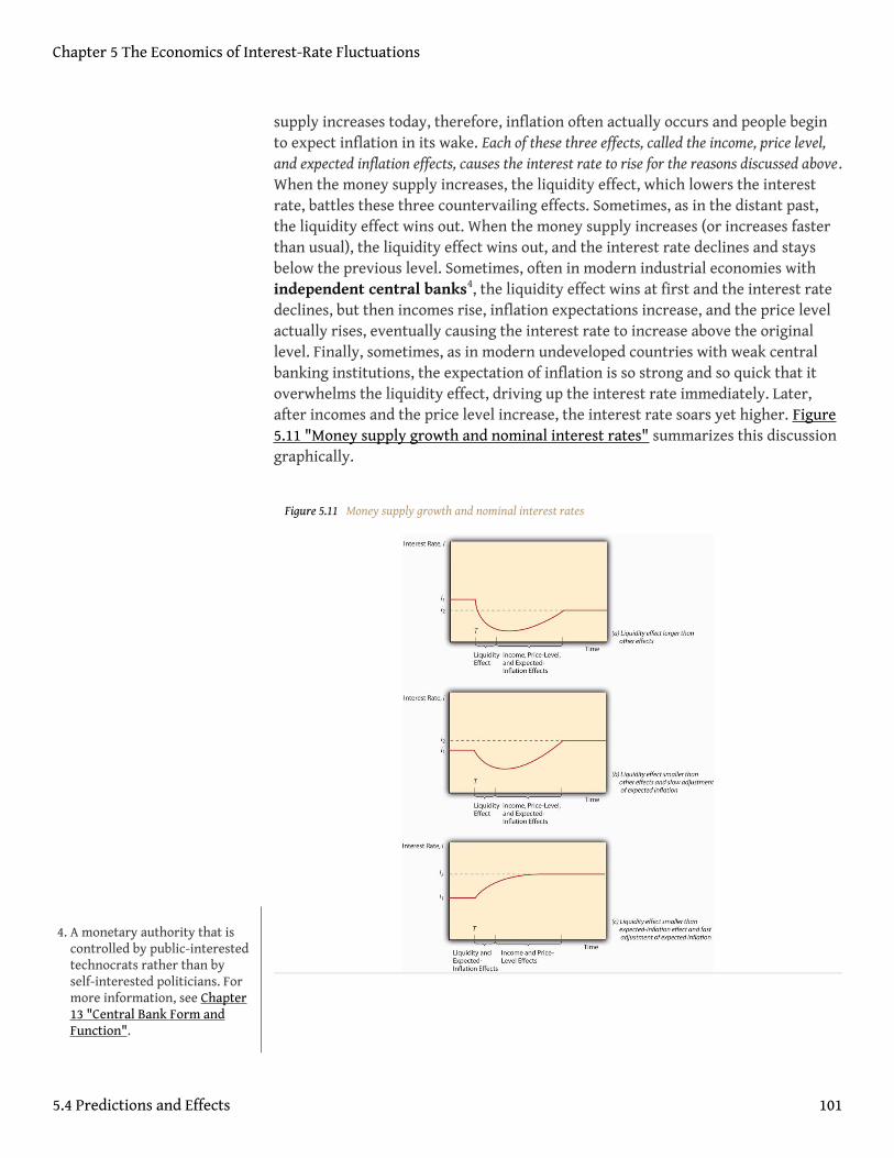
supply increases today, therefore, inflation often actually occurs and people beginto expect inflation in its wake. Each of these three effects, called the income, price level,and expected inflation effects, causes the interest rate to rise for the reasons discussed above.When the money supply increases, the liquidity effect, which lowers the interestrate, battles these three countervailing effects. Sometimes, as in the distant past,the liquidity effect wins out. When the money supply increases (or increases fasterthan usual), the liquidity effect wins out, and the interest rate declines and staysbelow the previous level. Sometimes, often in modern industrial economies withindependent central banks4, the liquidity effect wins at first and the interest ratedeclines, but then incomes rise, inflation expectations increase, and the price levelactually rises, eventually causing the interest rate to increase above the originallevel. Finally, sometimes, as in modern undeveloped countries with weak centralbanking institutions, the expectation of inflation is so strong and so quick that itoverwhelms the liquidity effect, driving up the interest rate immediately. Later,after incomes and the price level increase, the interest rate soars yet higher. Figure5.11 "Money supply growth and nominal interest rates" summarizes this discussiongraphically.
Figure 5.11 Money supply growth and nominal interest rates
4. A monetary authority that iscontrolled by public-interestedtechnocrats rather than byself-interested politicians. Formore information, see Chapter13 "Central Bank Form andFunction".
Chapter 5 The Economics of Interest-Rate Fluctuations
5.4 Predictions and Effects 101
Stop and Think Box
Famed monetary economist and Nobel laureate MiltonFriedmanhttp://www.econlib.org/library/Enc/bios/Friedman.html
By fixing the MS, the interest rate would have risen higher and higher as thedemand for money increased due to higher incomes and even simplepopulation growth. Only deflation (decreases in the price level) could havecountered that tendency, but deflation, Friedman knew, was as pernicious asinflation. A constant rate of MS growth, he believed, would keep the price levelrelatively stable and interest rate fluctuations less frequent or severe.
The ability to forecast changes in the interest rate is a rare but profitable gift. Professionalinterest rate forecasters are rarely right on the mark and often are farastray,www.finpipe.com/intratgo.htm and half the time they don’t even get the direction(up or down)right.taylorandfrancis.metapress.com/(vqspd445seikpajibz05ch45)/app/home/contribution.asp?referrer=parent&backto=issue,5,9;journal,15,86;linkingpublicationresults,1:100411,1 That’swhat we’d expect if their forecasts were determined by flipping a coin! We’ll discusswhy this might be in Chapter 7 "Rational Expectations, Efficient Markets, and theValuation of Corporate Equities". Therefore, we don’t expect you to be able topredict changes in the interest rate, but we do expect you to be able to post-dictthem. In other words, you should be able to narrate, in words and appropriategraphs, why past changes occurred. You should also be able to make predictions byinvoking the ceteris paribus assumption.
KEY TAKEAWAYS
• Under a commodity money system such as the gold standard, anincrease in the money supply decreases the interest rate and a decreasein the money supply increases it.
• Under a floating or fiat money system like we have today, an increase inthe money supply might induce interest rates to rise immediately ifinflation expectations were strong or to rise with a lag as actual inflationtook place.
Chapter 5 The Economics of Interest-Rate Fluctuations
5.4 Predictions and Effects 102
5.5 Suggested Reading
Bibow, Jorg. Keynes on Monetary Policy, Finance and Uncertainty: Reassessing LiquidityPreference Theory. New York: Routledge, 2009.
Evans, Michael. Practical Business Forecasting. Hoboken, NJ: John Wiley and Sons,2002.
Friedman, Milton. The Optimum Quantity of Money. Piscataway, NJ: AldineTransaction, 2005.
Chapter 5 The Economics of Interest-Rate Fluctuations
103
Chapter 6
The Economics of Interest-Rate Spreads and Yield Curves
CHAPTER OBJECTIVES
By the end of this chapter, students should be able to:
1. Define the risk structure of interest rates and explain its importance.2. Explain the term flight to quality.3. Define the term structure of interest rates and explain its importance.4. Describe a yield curve and explain its economic meaning.
104
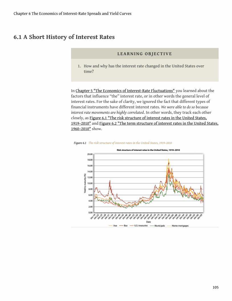
6.1 A Short History of Interest Rates
LEARNING OBJECTIVE
1. How and why has the interest rate changed in the United States overtime?
In Chapter 5 "The Economics of Interest-Rate Fluctuations" you learned about thefactors that influence “the” interest rate, or in other words the general level ofinterest rates. For the sake of clarity, we ignored the fact that different types offinancial instruments have different interest rates. We were able to do so becauseinterest rate movements are highly correlated. In other words, they track each otherclosely, as Figure 6.1 "The risk structure of interest rates in the United States,1919–2010" and Figure 6.2 "The term structure of interest rates in the United States,1960–2010" show.
Figure 6.1 The risk structure of interest rates in the United States, 1919–2010
Chapter 6 The Economics of Interest-Rate Spreads and Yield Curves
105
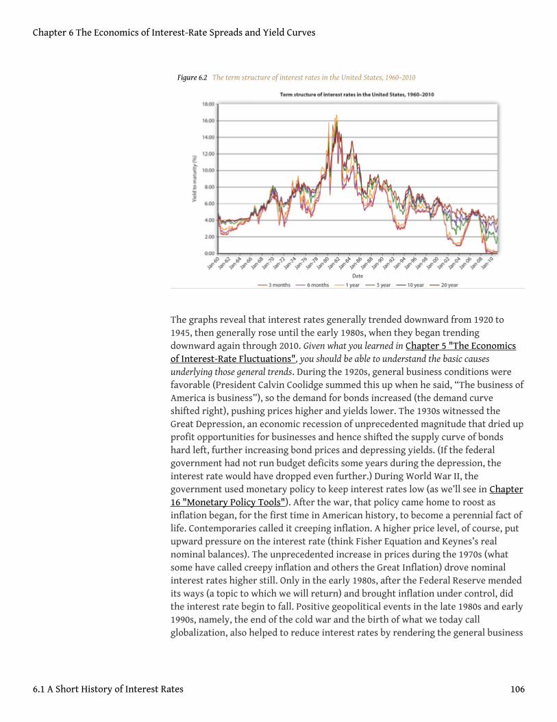
Figure 6.2 The term structure of interest rates in the United States, 1960–2010
The graphs reveal that interest rates generally trended downward from 1920 to1945, then generally rose until the early 1980s, when they began trendingdownward again through 2010. Given what you learned in Chapter 5 "The Economicsof Interest-Rate Fluctuations", you should be able to understand the basic causesunderlying those general trends. During the 1920s, general business conditions werefavorable (President Calvin Coolidge summed this up when he said, “The business ofAmerica is business”), so the demand for bonds increased (the demand curveshifted right), pushing prices higher and yields lower. The 1930s witnessed theGreat Depression, an economic recession of unprecedented magnitude that dried upprofit opportunities for businesses and hence shifted the supply curve of bondshard left, further increasing bond prices and depressing yields. (If the federalgovernment had not run budget deficits some years during the depression, theinterest rate would have dropped even further.) During World War II, thegovernment used monetary policy to keep interest rates low (as we’ll see in Chapter16 "Monetary Policy Tools"). After the war, that policy came home to roost asinflation began, for the first time in American history, to become a perennial fact oflife. Contemporaries called it creeping inflation. A higher price level, of course, putupward pressure on the interest rate (think Fisher Equation and Keynes’s realnominal balances). The unprecedented increase in prices during the 1970s (whatsome have called creepy inflation and others the Great Inflation) drove nominalinterest rates higher still. Only in the early 1980s, after the Federal Reserve mendedits ways (a topic to which we will return) and brought inflation under control, didthe interest rate begin to fall. Positive geopolitical events in the late 1980s and early1990s, namely, the end of the cold war and the birth of what we today callglobalization, also helped to reduce interest rates by rendering the general business
Chapter 6 The Economics of Interest-Rate Spreads and Yield Curves
6.1 A Short History of Interest Rates 106
climate more favorable (thus pushing the demand curve for bonds to the right,bond prices upward, and yields downward). Pretty darn neat, eh?
KEY TAKEAWAYS
• When general business conditions were favorable, demand for bondsincreased (the demand curve shifted right), pushing prices higher andyields lower.
• When general business conditions were unfavorable, profitopportunities for businesses dried up, shifting the supply curve of bondsleft, further increasing bond prices and depressing yields.
• During inflationary periods, interest rates rose per the Fisher Equationand Keynes’s real nominal balances.
• The end of the cold war and the birth of globalization helped to reduceinterest rates by rendering the general business climate more favorable(thus pushing the demand curve for bonds to the right, bond pricesupward, and yields downward).
Chapter 6 The Economics of Interest-Rate Spreads and Yield Curves
6.1 A Short History of Interest Rates 107
6.2 Interest-Rate Determinants I: The Risk Structure
LEARNING OBJECTIVE
1. What is the risk structure of interest rates and flight to quality, andwhat do they explain?
In this chapter, we’re going to figure out, as best we can, why yields on different types ofbonds differ. The analysis will help us to understand a couple of interesting featuresof Figure 6.1 "The risk structure of interest rates in the United States, 1919–2010"and Figure 6.2 "The term structure of interest rates in the United States,1960–2010":
1. Why the yields on Baa corporate bonds are always higher than theyields on Aaa corporate bonds, which in turn are higher than those onTreasury bonds (issued by the federal government), which for a longtime have been higher still than those on munis (bonds issued bymunicipalities, like state and local governments)
2. Why the yields on corporate Baa bonds bucked the trend of lower ratesin the early 1930s and why, at one time, municipal bonds yielded morethan Treasuries
3. Why bonds issued by the same economic entity (the U.S. government)with different maturities generally, but not always, have differentyields and why the rank ordering changes over time
Figure 6.1 "The risk structure of interest rates in the United States, 1919–2010",which holds maturity constant, is the easiest to understand because we’ve alreadydiscussed the major concepts. We’ll tackle it, and what economists call the riskstructure of interest rates, first. Remember from Chapter 5 "The Economics ofInterest-Rate Fluctuations" that investors care mostly about three things: risk,return, and liquidity. Because the bonds in Figure 6.1 "The risk structure of interestrates in the United States, 1919–2010" are all long-term bonds, their expectedrelative returns might appear at first glance to be identical. Investors know, however,that bonds issued by different economic entities have very different probabilities ofdefaulting. Specifically, they know the following:
1. The U.S. government has never defaulted on its bonds and is extremelyunlikely to do so because even if its much-vaunted political stabilitywere to be shattered and its efficient tax administration (that
Chapter 6 The Economics of Interest-Rate Spreads and Yield Curves
108

wonderful institution, the Internal Revenue Service [IRS]) were tostumble, it could always meet its nominal obligations by creatingmoney. (That might create inflation, as it has at times in the past.Nevertheless, except for a special type of bond called TIPS, thegovernment and other bond issuers promise to pay a nominal value,not a real [inflation-adjusted] sum, so the government does nottechnically default when it pays its obligations by printing money.)
2. Municipalities have defaulted on their bonds in the past and could doso again in the future because, although they have the power to tax,they do not have the power to create money at will. (Although in thepast, most recently during the Great Depression, some issued money-like—let’s call them extralegal—bills of credit, or chits.) Nevertheless,the risk of default on municipal bonds (aka munis) is often quite low,especially for revenue bonds, upon which specific taxes and fees arepledged for interest payments.
3. Munis are exempt from most forms of income taxation.4. Corporations are more likely to default on their bonds than
governments are because they must rely on business conditions andmanagement acumen. They have no power to tax and only a limitedability to create the less-liquid formsof money, a power that decreasesin proportion to their need! (I’m thinking of gift cards, decliningbalance debit cards, trade credit, and so forth.) Some corporations aremore likely to default on their bonds than others. Several credit-ratingagencies, including Moody’s and Standard and Poor’s, assess theprobability of default and assign grades to each bond. There is quite abit of grade inflation built in (the highest grade being not A or even A+but Aaa), the agencies are rife with conflicts of interest, and the marketusually senses problems before the agencies do. Nevertheless, bondratings are a standard proxy for default risk because, as Figure 6.3"Default rates on bonds rated by Moody’s from 1983 to 1999" shows,lower-rated bonds are indeed more likely to default than higher-ratedones. Like Treasuries, corporate bonds are fully taxable.
5. The most liquid bond markets are usually those for Treasuries. Theliquidity of corporate and municipal bonds is usually a function of thesize of the issuer and the amount of bonds outstanding. So the bonds ofthe state of New Jersey might be more liquid than those of a smallcorporation, but less liquid than the bonds of, say, General Electric.
Chapter 6 The Economics of Interest-Rate Spreads and Yield Curves
6.2 Interest-Rate Determinants I: The Risk Structure 109
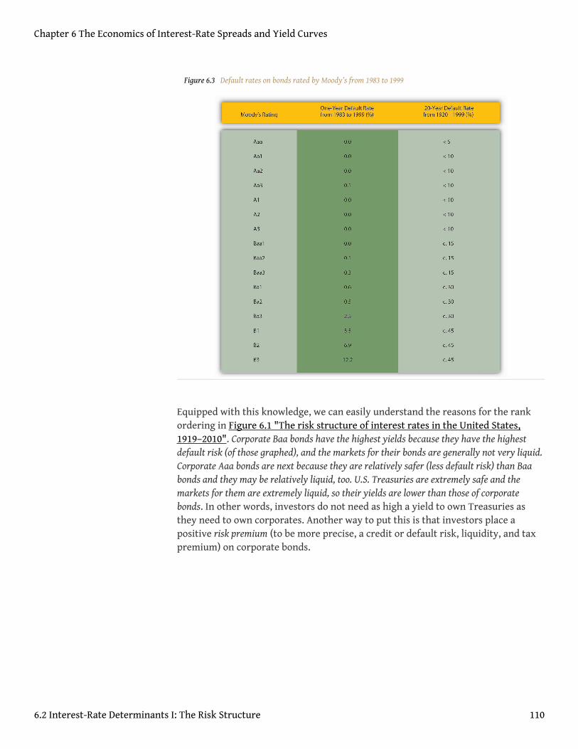
Figure 6.3 Default rates on bonds rated by Moody’s from 1983 to 1999
Equipped with this knowledge, we can easily understand the reasons for the rankordering in Figure 6.1 "The risk structure of interest rates in the United States,1919–2010". Corporate Baa bonds have the highest yields because they have the highestdefault risk (of those graphed), and the markets for their bonds are generally not very liquid.Corporate Aaa bonds are next because they are relatively safer (less default risk) than Baabonds and they may be relatively liquid, too. U.S. Treasuries are extremely safe and themarkets for them are extremely liquid, so their yields are lower than those of corporatebonds. In other words, investors do not need as high a yield to own Treasuries asthey need to own corporates. Another way to put this is that investors place apositive risk premium (to be more precise, a credit or default risk, liquidity, and taxpremium) on corporate bonds.
Chapter 6 The Economics of Interest-Rate Spreads and Yield Curves
6.2 Interest-Rate Determinants I: The Risk Structure 110
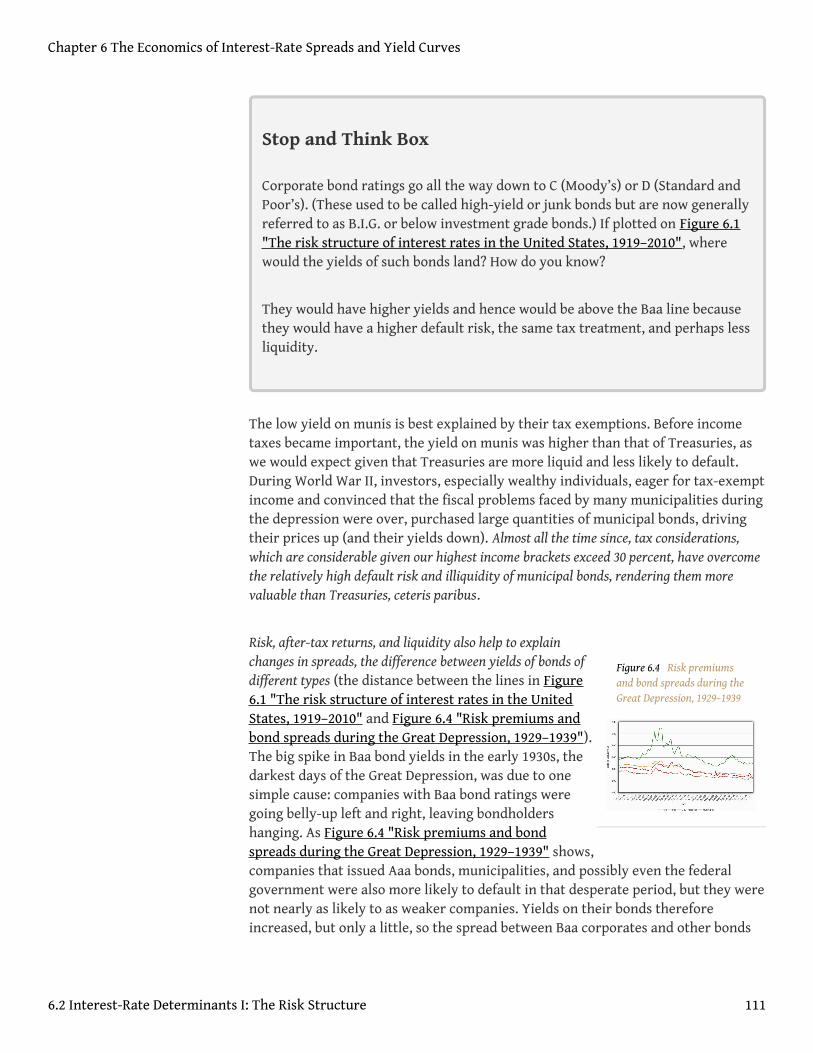
Figure 6.4 Risk premiumsand bond spreads during theGreat Depression, 1929–1939
Stop and Think Box
Corporate bond ratings go all the way down to C (Moody’s) or D (Standard andPoor’s). (These used to be called high-yield or junk bonds but are now generallyreferred to as B.I.G. or below investment grade bonds.) If plotted on Figure 6.1"The risk structure of interest rates in the United States, 1919–2010", wherewould the yields of such bonds land? How do you know?
They would have higher yields and hence would be above the Baa line becausethey would have a higher default risk, the same tax treatment, and perhaps lessliquidity.
The low yield on munis is best explained by their tax exemptions. Before incometaxes became important, the yield on munis was higher than that of Treasuries, aswe would expect given that Treasuries are more liquid and less likely to default.During World War II, investors, especially wealthy individuals, eager for tax-exemptincome and convinced that the fiscal problems faced by many municipalities duringthe depression were over, purchased large quantities of municipal bonds, drivingtheir prices up (and their yields down). Almost all the time since, tax considerations,which are considerable given our highest income brackets exceed 30 percent, have overcomethe relatively high default risk and illiquidity of municipal bonds, rendering them morevaluable than Treasuries, ceteris paribus.
Risk, after-tax returns, and liquidity also help to explainchanges in spreads, the difference between yields of bonds ofdifferent types (the distance between the lines in Figure6.1 "The risk structure of interest rates in the UnitedStates, 1919–2010" and Figure 6.4 "Risk premiums andbond spreads during the Great Depression, 1929–1939").The big spike in Baa bond yields in the early 1930s, thedarkest days of the Great Depression, was due to onesimple cause: companies with Baa bond ratings weregoing belly-up left and right, leaving bondholdershanging. As Figure 6.4 "Risk premiums and bondspreads during the Great Depression, 1929–1939" shows,companies that issued Aaa bonds, municipalities, and possibly even the federalgovernment were also more likely to default in that desperate period, but they werenot nearly as likely to as weaker companies. Yields on their bonds thereforeincreased, but only a little, so the spread between Baa corporates and other bonds
Chapter 6 The Economics of Interest-Rate Spreads and Yield Curves
6.2 Interest-Rate Determinants I: The Risk Structure 111
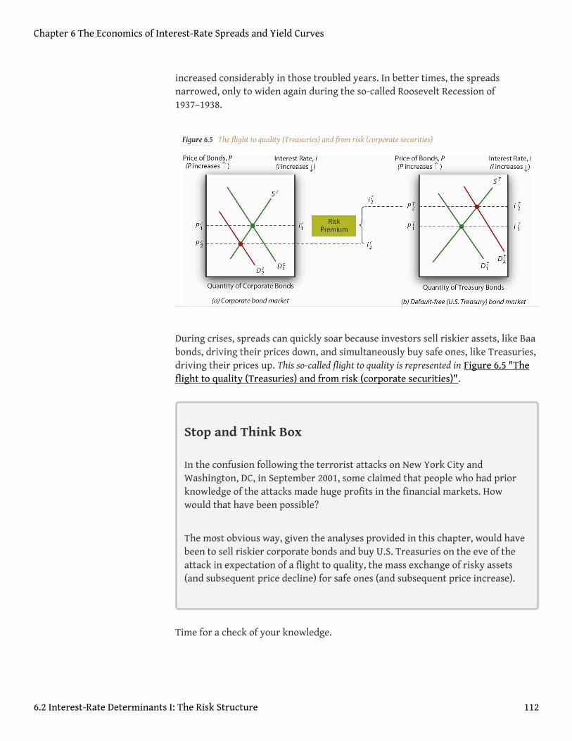
increased considerably in those troubled years. In better times, the spreadsnarrowed, only to widen again during the so-called Roosevelt Recession of1937–1938.
Figure 6.5 The flight to quality (Treasuries) and from risk (corporate securities)
During crises, spreads can quickly soar because investors sell riskier assets, like Baabonds, driving their prices down, and simultaneously buy safe ones, like Treasuries,driving their prices up. This so-called flight to quality is represented in Figure 6.5 "Theflight to quality (Treasuries) and from risk (corporate securities)".
Stop and Think Box
In the confusion following the terrorist attacks on New York City andWashington, DC, in September 2001, some claimed that people who had priorknowledge of the attacks made huge profits in the financial markets. Howwould that have been possible?
The most obvious way, given the analyses provided in this chapter, would havebeen to sell riskier corporate bonds and buy U.S. Treasuries on the eve of theattack in expectation of a flight to quality, the mass exchange of risky assets(and subsequent price decline) for safe ones (and subsequent price increase).
Time for a check of your knowledge.
Chapter 6 The Economics of Interest-Rate Spreads and Yield Curves
6.2 Interest-Rate Determinants I: The Risk Structure 112
EXERCISES
1. What would happen to the spreads between different types of bonds ifthe federal government made Treasuries tax-exempt and at the sametime raised income taxes considerably?
2. If the Supreme Court unexpectedly declared a major source of municipalgovernment tax revenue illegal, what would happen to municipal bondyields?
3. If several important bond brokers reduced the brokerage fee theycharge for trading Baa corporate bonds (while keeping their fees forother bonds the same), what would happen to bond spreads?
4. What happened to bond spreads when Enron, a major corporation,collapsed in December 2001?
KEY TAKEAWAYS
• The risk structure of interest rates explains why bonds of the samematurity but issued by different economic entities have different yields(interest rates).
• The three major risks are default, liquidity, and after-tax return.• By concentrating on the three major risks, you can ascertain why some
bonds are more (less) valuable than others, holding their term(repayment date) constant.
• You can also post-dict, if not outright predict, the changes in rank orderas well as the spread (or difference in yield) between different types ofbonds.
• A flight to quality occurs during a crisis when investors sell risky assets(like below-investment-grade bonds) and buy safe ones (like Treasurybonds or gold).
Chapter 6 The Economics of Interest-Rate Spreads and Yield Curves
6.2 Interest-Rate Determinants I: The Risk Structure 113
6.3 The Determinants of Interest Rates II: The Term Structure
LEARNING OBJECTIVE
1. What is the term structure of interest rates and the yield curve, andwhat do they explain?
Now we are going to hold the risk structure of interest rates—default risk, liquidity, andtaxes—constant and concentrate on what economists call the term structure of interestrates, the variability of returns due to differing maturities. As Figure 6.4 "Risk premiumsand bond spreads during the Great Depression, 1929–1939" reveals, even bondsfrom the same issuer, in this case, the U.S. government, can have yields that varyaccording to the length of time they have to run before their principals are repaid.Note that the general postwar trend is the same as that in Figure 6.1 "The riskstructure of interest rates in the United States, 1919–2010", a trend upwardfollowed by an equally dramatic slide. Unlike Figure 6.1 "The risk structure ofinterest rates in the United States, 1919–2010", however, the ranking of the serieshere is much less stable. Sometimes short-term Treasuries have lower yields thanlong-term ones, sometimes they have about the same yield, and sometimes theyhave higher yields.
To study this phenomenon more closely, economists and market watchers use a toolcalled a yield curve, which is basically a snapshot of yields of bonds of differentmaturities at a given moment. Figure 6.1 "The risk structure of interest rates in theUnited States, 1919–2010" is what the Treasury yield curve looks like as reported inthe Wall Street Journal, which publishes it daily. The current yield curve can also beviewed many places online, including Bloomberg and the U.S. Treasuryitself.www.bloomberg.com/markets/rates/index.html;http://www.ustreas.gov/offices/domestic-finance/debt-management/interest-rate/yield.shtml Whatobservers have discovered is that the yields of bonds of different maturities (but identicalrisk structures) tend to move in tandem. They also note that yield curves usually slopeupward. In other words, short-term rates are usually lower than long-term rates. Sometimes,however, the yield “curve” is actually flat—yields for bonds of different maturities areidentical, or nearly so. Sometimes, particularly when short-term rates are higher thannormal, the curve inverts or slopes downward, indicating that the yield on short-term bondsis higher than that on long-term bonds. And sometimes the curve goes up and down,resembling a sideways S (sometimes tilted on its face and sometimes its back) or Z. Whatexplains this? (Remember, it can’t be tax, default, or liquidity risk because thosevariables are all the same for Treasuries.)
Chapter 6 The Economics of Interest-Rate Spreads and Yield Curves
114

Figure 6.6 Treasury yieldcurve
Theory and empirical evidence both point to the sameconclusion: bonds of different maturities are partialsubstitutes for each other, not perfect substitutes, but notcompletely segmented either. Generally, investors prefershort-term bonds to long-term ones, but they reverse theirpreference if the interest rate goes unusually high. Investorsare willing to pay more for short-term bonds, otherfactors (like “the” interest rate and the risk structure)held constant, because longer-term bonds are moresubject to interest rate risk, as we learned in Chapter 3"Money". Or, to put it another way, investors need apremium (in the form of a lower price or higher yield)to hold long-term bonds. Ergo, the yield curve usuallyslopes upward, as it does in Figure 6.6 "Treasury yieldcurve".
But what about those times when the curve is flat orinverted? Well, there is one thing that can induceinvestors to give up their liquidity preference1, their preferred habitat2 of short-term bonds: the expectation of a high interest rate for a short term. Investors think ofa long-term bond yield as the average of the yields on shorter-term obligations, so when theinterest rate is high by historical norms but expected after a year or so to revert to somelong-term mean, they will actually begin to prefer long-term bonds and will buy them atmuch higher prices (lower yields) than short-term bonds. More formally, investorsbelieve that
where:
in = interest rate today on a bond that matures in n years
iex = expected interest rate at time x (0, 1, 2, 3, . . . through n)
ρ = the liquidity or term premium for an n-period bond (it is always positive andincreases with n)
So the yield today of a bond with 5 years to maturity, if the liquidity premium is .5percent and the expected interest rate each year is 4, is 4.5:
in = [(ie0 + ie1 + ie2 + ie3 + .... ie (n−1) )/n] + ρn
1. The name of one of thetheories that economists use toexplain the yield curve.
2. The name of one of thetheories that economists use toexplain the yield curve.
Chapter 6 The Economics of Interest-Rate Spreads and Yield Curves
6.3 The Determinants of Interest Rates II: The Term Structure 115
i5 = (4 + 4 + 4 + 4 + 4)/5 + .5 = 20/5 + .5 = 4.5, implying an upward sloping yield curve
because 4 < 4.5.
If the interest rate is expected to rise over the next 5 years, the yield curve slopesupward yet more steeply:
i5 = (4 + 5 + 6 + 7 + 8)/5 + .5 = 30/5 + .5 = 6.5, again implying an upward sloping curve
because 4 < 6.5.
If, on the other hand, interest rates are expected to fall over the next 5 years, theyield curve will slope downward, as in this example:
i5 = (12 + 10 + 8 + 5 + 5)/5 + .5 = 40/5 + .5 = 8.5, implying an inverted yield curve
because 12 > 8.5.
Investors may also realize that long-term bonds will increase in price when interestrates fall (as they are expected to do in this example and as we learned in Chapter 3"Money"), so they are willing to pay more for them now.
Stop and Think Box
In the nineteenth century, the yield curve was usually flat under normalconditions. (It inverted during financial panics.) In other words, short-term andlong-term bonds issued by the same economic entity did not often differ muchin price. Why might that have been?
One possibility is that there was no liquidity premium then. Then, as now,short-term bonds suffered less interest rate risk than long-term bonds, butinvestors often complained of extremely high levels of reinvestment risk, oftheir inability to easily and cheaply reinvest the principal of bonds andmortgages when they were repaid. Often, lenders urged good borrowers not torepay (but to continue to service their obligations, of course). Another notmutually exclusive possibility is that the long-term price level stabilityengendered by the specie standard made the interest rate less volatile. Theexpectation was that the interest rate would not long stray from its long-termtendency.
Chapter 6 The Economics of Interest-Rate Spreads and Yield Curves
6.3 The Determinants of Interest Rates II: The Term Structure 116
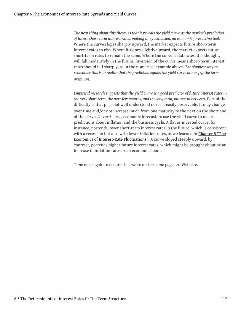
The neat thing about this theory is that it reveals the yield curve as the market’s predictionof future short-term interest rates, making it, by extension, an economic forecasting tool.Where the curve slopes sharply upward, the market expects future short-terminterest rates to rise. Where it slopes slightly upward, the market expects futureshort-term rates to remain the same. Where the curve is flat, rates, it is thought,will fall moderately in the future. Inversion of the curve means short-term interestrates should fall sharply, as in the numerical example above. The simplest way toremember this is to realize that the prediction equals the yield curve minus ρn, the term
premium.
Empirical research suggests that the yield curve is a good predictor of future interest rates inthe very short term, the next few months, and the long term, but not in between. Part of thedifficulty is that ρn is not well understood nor is it easily observable. It may change
over time and/or not increase much from one maturity to the next on the short endof the curve. Nevertheless, economic forecasters use the yield curve to makepredictions about inflation and the business cycle. A flat or inverted curve, forinstance, portends lower short-term interest rates in the future, which is consistentwith a recession but also with lower inflation rates, as we learned in Chapter 5 "TheEconomics of Interest-Rate Fluctuations". A curve sloped steeply upward, bycontrast, portends higher future interest rates, which might be brought about by anincrease in inflation rates or an economic boom.
Time once again to ensure that we’re on the same page, er, Web site.
Chapter 6 The Economics of Interest-Rate Spreads and Yield Curves
6.3 The Determinants of Interest Rates II: The Term Structure 117
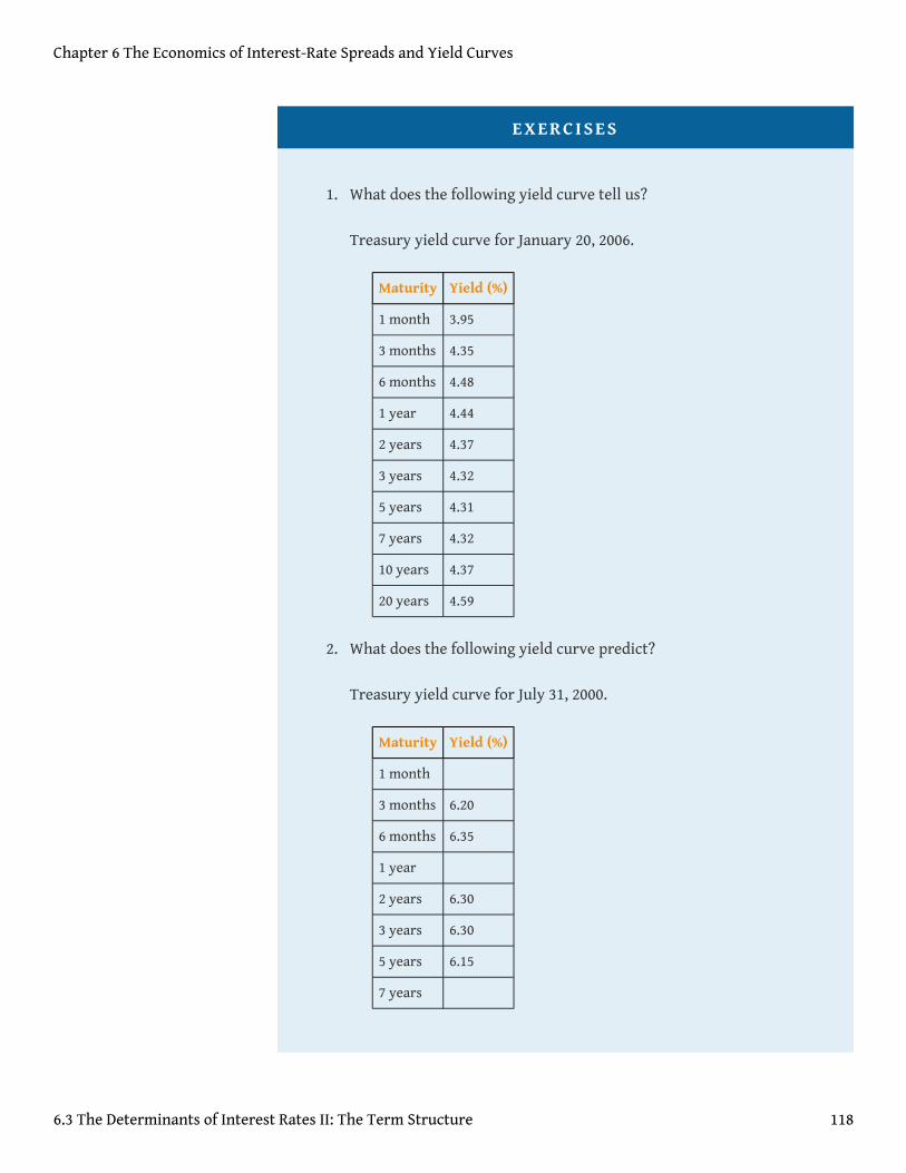
EXERCISES
1. What does the following yield curve tell us?
Treasury yield curve for January 20, 2006.
Maturity Yield (%)
1 month 3.95
3 months 4.35
6 months 4.48
1 year 4.44
2 years 4.37
3 years 4.32
5 years 4.31
7 years 4.32
10 years 4.37
20 years 4.59
2. What does the following yield curve predict?
Treasury yield curve for July 31, 2000.
Maturity Yield (%)
1 month
3 months 6.20
6 months 6.35
1 year
2 years 6.30
3 years 6.30
5 years 6.15
7 years
Chapter 6 The Economics of Interest-Rate Spreads and Yield Curves
6.3 The Determinants of Interest Rates II: The Term Structure 118
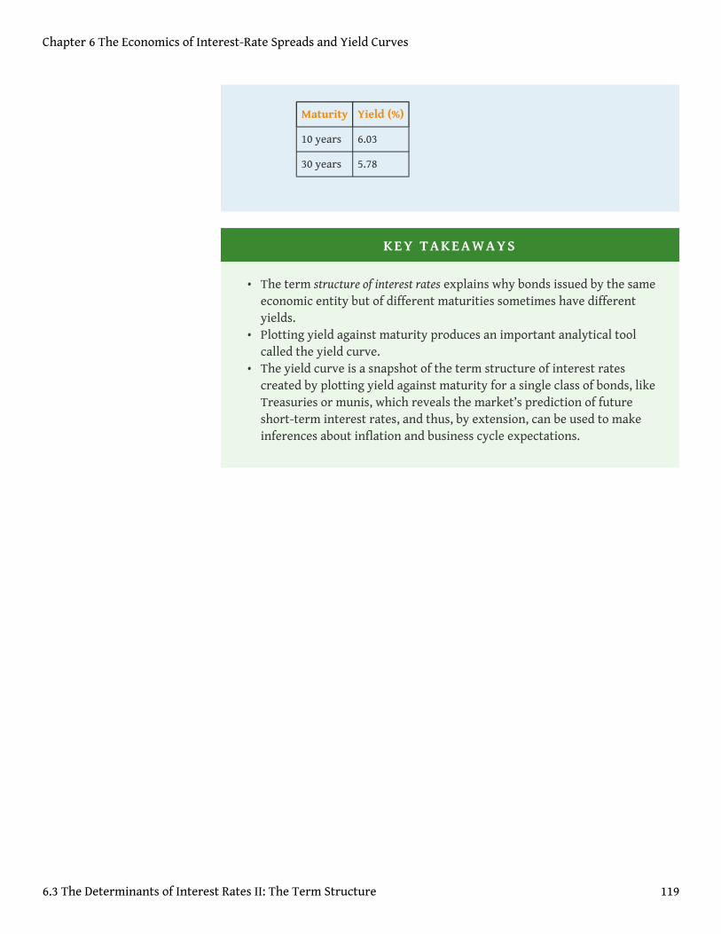
Maturity Yield (%)
10 years 6.03
30 years 5.78
KEY TAKEAWAYS
• The term structure of interest rates explains why bonds issued by the sameeconomic entity but of different maturities sometimes have differentyields.
• Plotting yield against maturity produces an important analytical toolcalled the yield curve.
• The yield curve is a snapshot of the term structure of interest ratescreated by plotting yield against maturity for a single class of bonds, likeTreasuries or munis, which reveals the market’s prediction of futureshort-term interest rates, and thus, by extension, can be used to makeinferences about inflation and business cycle expectations.
Chapter 6 The Economics of Interest-Rate Spreads and Yield Curves
6.3 The Determinants of Interest Rates II: The Term Structure 119
6.4 Suggested Reading
Choudry, Moorad. Analysing and Interpreting the Yield Curve. Hoboken, NJ: John Wileyand Sons, 2004.
Fabozzi, Frank. Interest Rate, Term Structure, and Valuation Modeling. Hoboken, NJ:John Wiley and Sons, 2002.
Fabozzi, Frank, Steven Mann, and Moorad Choudry. Measuring and Controlling InterestRate and Credit Risk. Hoboken, NJ: John Wiley and Sons, 2003.
Homer, Sidney, and Richard E. Sylla. A History of Interest Rates, 4th ed. Hoboken, NJ:John Wiley and Sons, 2005.
Chapter 6 The Economics of Interest-Rate Spreads and Yield Curves
120
Chapter 7
Rational Expectations, Efficient Markets, and the Valuation ofCorporate Equities
CHAPTER OBJECTIVES
By the end of this chapter, students should be able to:
1. Explain when expectations are rational and when they are irrational.2. Explain how corporate equities (stocks, shares of a corporation) are
valued.3. Explain what is meant by the term market efficiency.4. Describe the ways in which financial markets are efficient.5. Describe the ways in which financial markets are inefficient.
121
7.1 The Theory of Rational Expectations
LEARNING OBJECTIVE
1. When are expectations rational and when are they irrational?
Market volatility1, the constantly changing prices of financialinstruments,www.cboe.com/micro/vix/introduction.aspx tricks some people intothinking that financial markets, especially stock markets, are flim-flams or giganticroulette wheels. Stock prices, they suspect, are at best random and at worst rigged.In fact, financial markets are more efficient, and hence fairer, than other markets. Thedirection of price movements (up or down) is indeed random, but price levels arebased on the rational expectations2 of a large number of market participants.While financial scams certainly exist, the stock and bond markets are not rigged.Except perhaps for some penny stocks, securities prices are usually based oneconomic fundamentals3 and are not systematically manipulated by insiders orconspirators. Investing in corporate equities certainly entails risk, but it is not akinto playing the lottery. Luck can play a role in investing, as in anything in life, butunlike a Powerball drawing, Lady Luck is not the whole of the game by a long shot.Far from being gamblers, investors4 are switches in the most advanced computingdevices in the history of the world, financial markets. Prices in those markets helpto determine what gets made and what doesn’t, how much gets produced and how,and where and how those goods are sold.
Financial markets, in the world’s most economically advanced countries anyway,have been rational and efficient decision-making machines for many centuries. In1688, a broker in Amsterdam, Netherlands, named Joseph de la Vega, left posteritywith vivid descriptions of the Dutch securities market.en.wikipedia.org/wiki/Joseph_Penso The market, he claimed, was just a game of misinformation and spinmanagement that pitted bulls (those who profited from an increase in prices)against bears (those who profited from a decrease in prices):
“The bulls are like the giraffe which is scared by nothing. . . . They love everything,they praise everything, they exaggerate everything. . . . The bulls make the publicbelieve that their tricks signify wealth and that crops grow on graves. Whenattacked by serpents, they . . . regard them as both a delicate and a delicious meal. .. . They are not impressed by a fire nor perturbed by a debacle. . . . The bears, on thecontrary, are completely ruled by fear, trepidation, and nervousness. Rabbitsbecome elephants, brawls in a tavern become rebellions, faint shadows appear to
1. In this context, frequentchanges in securities prices.
2. An economic theory that positsthat market participants, inthis case investors, input allavailable relevant informationinto the best forecasting modelavailable.
3. Key variables in the pricing ofassets. They include expectedinflation, interest, default, andearnings rates.
4. Participants in financialmarkets; purchasers offinancial securities.
Chapter 7 Rational Expectations, Efficient Markets, and the Valuation of Corporate Equities
122
them as signs of chaos. . . . What is there miraculous about the likelihood that everydwarf will become a giant in the eyes of the bears?”Joseph de la Vega, Confusion deConfusiones.
Joseph de la Vega went on to detail a dozen different ways in which cabals of bearsand herds of bulls tried to influence securities prices. The net effect of suchmachinations, though, was unclear. Sometimes the bulls won, sometimes the bearswon, but their activities often canceled each other out. “Numerous brokers areinexhaustible in inventing involved maneuvers,” de la Vega explained, “but for justthis reason do not achieve their purposes.” Systematic manipulation of the marketwas impossible because the bulls and bears competed against each other, eachtugging at the price, but ultimately in vain. Also, as rational investors learned thetricks of trading, they came to expect hyperbole, false rumors, sham sales, and thelike. So, in the final analysis, market fundamentals, not the whims of nefariousindividuals, determined prices. Exactly the same could be said of most of today’ssecurities markets. Generally speaking, stock and other securities prices fluctuate due togenuine changes in supply or demand, not because of the machinations of bulls and bears.
Joseph de la Vega’s 300+-year-old description of what was then the world’s mostadvanced securities market also made clear that expectations, rather than actualities,moved prices. “The expectation of an event,” he noted, “creates a much deeperimpression upon the exchange than the event itself.” As noted in the precedingchapters, expectations are still paramount today. People invest based on what theybelieve the future will bring, not on what the present brings or the past haswrought, though they often look to the present and past (sometimes even thedistant past) for clues about the future.
Rational expectations theory posits that investor expectations will be the best guessof the future using all available information. Expectations do not have to be correctto be rational; they just have to make logical sense given what is known at anyparticular moment. An expectation would be irrational if it did not logically followfrom what is known or if it ignored available information. For the former reason,investors expend considerable sums on schooling, books, lectures, seminars, andthe like, to learn the best ways to reason correctly given certain types ofinformation. (This textbook and course are a good start, but competition for thebest model5 is keen. Investment models and strategies constantly morph, adaptingto changes in the real world.) For the latter reason, investors update theirexpectations, or forecasts, with great frequency, as new information becomesavailable, which occurs basically 24/7/365.
If everyone’s expectations are rational, then why don’t investors agree on howmuch assets are worth? One investor may think gold6 a steal at $900/ounce, while
5. In this context, a theory aboutthe most accurate way to pricesecurities or to estimate thevalue of future variables suchas interest rates, risk, earnings,and other fundamentals.
6. At one time, gold was money,that is, the unit of accountagainst which the value of allgoods was measured. It is nowjust a precious metal thattrades on world markets likeother commodities, its pricerising and falling with shifts insupply and demand.
Chapter 7 Rational Expectations, Efficient Markets, and the Valuation of Corporate Equities
7.1 The Theory of Rational Expectations 123
another wouldn’t touch the stuff for a penny over $750. One investor might think$943.40 just right for a zero coupon bond7, but another might think it a good dealonly at $942.51. One may think that XYZ stock is overpriced at $22.57 a share, whileanother would buy a small quantity of it at that price, and yet another would buy allshe could at that price. Such differences in valuation are important because they allowtrades to occur by inducing some investors to sell and others to buy.
As it turns out, investors sometimes have different sets of information available to them.Some investors may have inside information8, news that is unknown outside asmall circle. Others may lack certain types of information because they think it istoo costly to obtain. Other times, investors think of the information they know incommon differently because their utility functions (their goals and aspirations, if you will)differ. So they have different time horizons, different holding periods, and differentsensitivities to risk.
At yet other times, investors use different valuation models9, different theories ofhow to predict fundamentals most accurately and how those fundamentalsdetermine securities prices. For example, some investors foresee long causal chainsmore clearly than other investors do. Recall from Chapter 5 "The Economics ofInterest-Rate Fluctuations" that the demand for asset X is partly a function of itsexpected return relative to all assets not-X. So investors must consider informationdirectly related to asset X and all other assets. A new piece of information half aworld away that alters expectations about a nation’s ability to repay its debts, asector’s future prospects, or a single company’s profits regularly ripples throughthe entire financial world. Ripple indeed evokes the right metaphor. Like throwinga pebble into a pond, the disruption is greatest at the epicenter, the spot where therock hits the water, but it dissipates over time and space. The bigger the pebble (thebigger the news), the bigger the splash and the larger and longer lasting thedisruption. Most days, the world’s financial pond is pelted with millions of littlepebbles, little pieces of news that cause prices to jiggle up and down. Every now andagain, a big stone, even a boulder, hits the pond, causing significant price changesthroughout the pond for quite a long time. (Economists call such boulders shocks,and they include financial crises like that of 2007–2008. Financial crises almostalways follow asset bubbles10, which we will discuss in more detail below.)
Some investors understand the effect of some ripples more quickly and clearly thanothers. This shouldn’t be taken to mean that some investors are smarter thanothers, only that they understand the types of ripples particular pebbles will makebetter than others do. The roles could reverse with the next pebble, with the nextbit of news. Moreover, investors constantly strive to improve their understandingof the ways that certain types of news affect securities prices. They emulatesuccessful people and develop new models and theories of their own, not for the joyof learning but for the clink of cold hard cash. For example, investors who
7. A discount bond that pays nocoupon or interest. Theinterest is earned by thedifference between the bond”sface or par value and the priceat which it is sold.
8. Information relevant to thevaluation of stock or othersecurity and known only to asmall group of people.
9. Theories of securities pricesand their determinants.
10. In this context, a rapid increasein asset prices that is not easilyjustified by fundamentals likeexpected earnings, interestrates, and the like.
Chapter 7 Rational Expectations, Efficient Markets, and the Valuation of Corporate Equities
7.1 The Theory of Rational Expectations 124
understood that oil prices hitting $50 per barrel would increase the share price ofhome insulation manufacturers merely stayed up with the crowd. It’s prettyobvious that higher home heating costs would induce people to buy insulation. Theinvestors who quickly figured out that the share price of a Canadian shinglemanufacturer would jump too were the ones that earned above-market returns.(High oil prices made it profitable to extract oil from Canada’s oil sand fields, butnot enough people lived in the area around Fort McMurray, Alberta, to meet labordemands. People flocking to the region to work needed new homes, the roofs ofwhich needed shingles, lots of them. www.npr.org/templates/story/story.php?storyId=6098557;http://www.iht.com/articles/2007/01/10/bloomberg/bxfort.php)
For all those reasons, investors often have a wide variety of opinions about thevalue of different assets. More mechanically, investors might have differentopinions about bond valuations because they must have different views about theapplicable discount or interest rate. To review,
If this is a one-year zero coupon bond, FV = $1,000, and i = 6%, then the bond price =($1,000/1.06) = $943.40. But if one believes i = 6.01, then the bond price = ($1,000/1.0601) = $942.51. To understand how investors can value the same stockdifferently, we must investigate how they value corporate equities.
KEY TAKEAWAYS
• Expectations are rational when they logically follow from all availablerelevant information.
• Expectations are irrational if some available pertinent information isignored or if conclusions do not flow logically from availableinformation.
PV = FV/(1 + i)n
Chapter 7 Rational Expectations, Efficient Markets, and the Valuation of Corporate Equities
7.1 The Theory of Rational Expectations 125
7.2 Valuing Corporate Equities
LEARNING OBJECTIVE
1. How are corporate equities valued?
A corporate equity, or stock, is sometimes called a share because it is just that, ashare in the ownership of a joint-stock corporation. Ownership entitles investors toa say in how the corporation is run. Today that usually means one vote per share incorporate elections for the board of directors, a group of people who direct,oversee, and monitor the corporation’s professional managers. Ownership also meansthat investors are residual claimants, entitling them to a proportionate share of thecorporation’s net earnings (profits), its cash flows, and its assets once all other claims againstit have been settled.
In exchange for their investment, stockholders11 may receive a flow of cashpayments, usually made quarterly, called dividends12. Dividends differ from bondcoupons in important ways. Unlike coupons, they are not fixed. They may go up ordown over time. Also, if a company fails to pay dividends on its stock, it is notconsidered in default. (We speak here of common stock. Another type of financialinstrument, a preferred share [preference shares in the United Kingdom], promisesto pay a fixed dividend. Such instruments are a type of equity-debt hybrid and arepriced more like coupon bonds.) In fact, many corporations today do not pay anydividends, and for good reasons. Small, rapidly growing companies, it is widelybelieved, should plow their profits back into their businesses rather than returnmoney to shareholders. That is not cheating the stockholders, because profits left with thecompany instead of paid out as dividends raise the share price. The company has morecash than it otherwise would, after all, and stockholders own the profits whetherthey are left with the company or put into their pockets. Plus, it is generallythought that growing companies put the money to more profitable use thanstockholders could.
There is a tax benefit to retaining earnings, too. Taxes on dividends, which theInternal Revenue Service (IRS)13 considers income, are usually higher than taxeson share appreciation, which the IRS considers capital gains.www.irs.gov/ Also,dividends are taxed in the year they are paid, which may be inconvenient forstockholders, but capital gains taxes are incurred only when the stockholders selltheir shares, so they have more control over their tax liabilities. Similarly,companies that have stopped growing will sometimes buy their own stock in the
11. Owners of corporate equities.Generally, they are entitled toone vote per share in corporateelections for directors and aproportionate share of thecorporation’s profits.
12. In this context, cashdistributions of corporateearnings to shareholders.
13. The tax collector of the U.S.federal government.
Chapter 7 Rational Expectations, Efficient Markets, and the Valuation of Corporate Equities
126
market rather than pay dividends. Fewer shares outstanding means that each shareis worth more (the price per share equals the total value of the company divided bythe number of shares, so as the denominator declines, the price per shareincreases), so stockholders are “paid” with a higher stock price. Nevertheless, somecorporations continue to pay dividends. The point here is that what really matters whenvaluing corporate equities is earnings or profits because, as noted above, they belong to thestockholders whether they are divided, kept as cash, or used to repurchase shares.
The simplest stock valuation method, the one-period valuation model, simply calculates thediscounted present value of earnings and selling price over a one-year holding period:
where:
P = price now
E = yearly earnings or profit
k = required rate of return
P? = expected price at year’s end
So if a company is expected to earn no profit, its share price is expected to be $75 atthe end of the year, and the required rate of return14 on investments in its riskclass is 10 percent, an investor would buy the stock if its market price was at orbelow P = 0/1.10 + 75/1.10 = $68.18. Another investor might also require a 10percent return but think the stock will be worth $104 at the end of the year. He’dpay P = 0/1.10 + 104/1.1 = $94.55 for the stock today! A third investor might agreewith the first, that the stock will be worth $75 in a year, but she might need a 12percent return. She’d pay only up to P = 0/1.12 + 75/1.12 = $66.96 per share. Yetanother investor might also require a 12 percent return to hold the stock and think$75 a reasonable price a year from now, but he might also think earnings of $1 pershare is in the offing. He’d pay P = 1/1.12 + 75/1.12 = .89 + 66.96 = $67.85 per share.
For longer holding periods, one can use the generalized dividend valuation model, whichdiscounts expected future earnings to their present value. That can be donemechanically, as we did for coupon bonds in Chapter 4 "Interest Rates", or with alittle fancier math:
P = E/(1 + k) + P1 /(1 + k)
14. Serves the same purpose as i inpresent value calculations. Inother words, it measures theopportunity cost of making aninvestment; k is influenced by ibut also by default and otherrisks.
Chapter 7 Rational Expectations, Efficient Markets, and the Valuation of Corporate Equities
7.2 Valuing Corporate Equities 127

That sideways 8 means infinity. So this equation basically says that the price of ashare now is the sum (σ) of the discounted present values of the expected earningsbetween now and infinity. The neat thing about this equation is that the expectedfuture sales price of the stock drops out of the equation because the present valueof any sum at any decent required rate of return quickly becomes negligible. (Forexample, the present value of an asset expected to be worth $10 in 20 years at 15percent interest is only PV = 10/(1.15)20 = $0.61 today.) So for all intents andpurposes in this model, a corporate equity is worth the discounted present value of itsexpected future earnings stream.
where
P= price today
E = most recent earnings
k = required return
g = constant growth rate
So the price of a stock today that recently earned $1 per share and has expectedearnings growth of 5 percent would be $21.00 if the required return was 10 percent(P = 1.05/.05). If another investor estimates either k or g differently, perhapsbecause he knows more (or less) about a country, industry, or company’s futureprospects, P will of course change, perhaps radically. For a little practice, completethe following exercises now.
P = t = 1∞Et/1 + kt
P = E(1 + g)/(k − g)
Chapter 7 Rational Expectations, Efficient Markets, and the Valuation of Corporate Equities
7.2 Valuing Corporate Equities 128
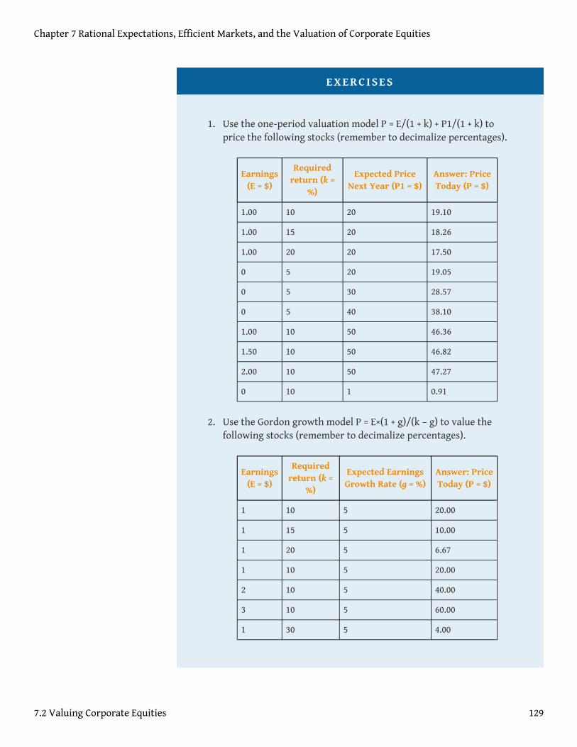
EXERCISES
1. Use the one-period valuation model P = E/(1 + k) + P1/(1 + k) toprice the following stocks (remember to decimalize percentages).
Earnings(E = $)
Requiredreturn (k =
%)
Expected PriceNext Year (P1 = $)
Answer: PriceToday (P = $)
1.00 10 20 19.10
1.00 15 20 18.26
1.00 20 20 17.50
0 5 20 19.05
0 5 30 28.57
0 5 40 38.10
1.00 10 50 46.36
1.50 10 50 46.82
2.00 10 50 47.27
0 10 1 0.91
2. Use the Gordon growth model P = E×(1 + g)/(k – g) to value thefollowing stocks (remember to decimalize percentages).
Earnings(E = $)
Requiredreturn (k =
%)
Expected EarningsGrowth Rate (g = %)
Answer: PriceToday (P = $)
1 10 5 20.00
1 15 5 10.00
1 20 5 6.67
1 10 5 20.00
2 10 5 40.00
3 10 5 60.00
1 30 5 4.00
Chapter 7 Rational Expectations, Efficient Markets, and the Valuation of Corporate Equities
7.2 Valuing Corporate Equities 129
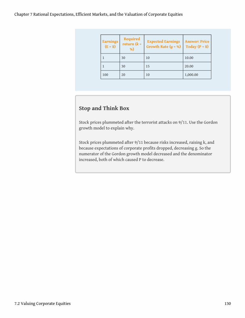
Earnings(E = $)
Requiredreturn (k =
%)
Expected EarningsGrowth Rate (g = %)
Answer: PriceToday (P = $)
1 30 10 10.00
1 30 15 20.00
100 20 10 1,000.00
Stop and Think Box
Stock prices plummeted after the terrorist attacks on 9/11. Use the Gordongrowth model to explain why.
Stock prices plummeted after 9/11 because risks increased, raising k, andbecause expectations of corporate profits dropped, decreasing g. So thenumerator of the Gordon growth model decreased and the denominatorincreased, both of which caused P to decrease.
Chapter 7 Rational Expectations, Efficient Markets, and the Valuation of Corporate Equities
7.2 Valuing Corporate Equities 130

KEY TAKEAWAYS
• In general, corporate equities are valued the same way that any financialsecurity is, by discounting expected future cash flows.
• With stocks, corporate earnings replace actual cash payments becauseshareholders own profits, whether they receive them as cash dividendsor not.
• The formula for valuing a stock to be held one year, called the one-period valuation model, is P = E/(1 + k) + P1/(1 + k), where E is expectedearnings, P1 is the expected sales price of the stock next year, and k isthe return required to hold the stock given its risk and liquiditycharacteristics.
• In the Gordon growth model, earnings are assumed to grow at aconstant rate forever, so stock values can be estimated without guessingthe future sales price by using the following formula: P = E(1 + g)/(k – g),where E = the most recent earnings, g = the rate of earnings growth, k =the required return where k > g.
Chapter 7 Rational Expectations, Efficient Markets, and the Valuation of Corporate Equities
7.2 Valuing Corporate Equities 131
7.3 Financial Market Efficiency
LEARNING OBJECTIVE
1. In what senses can financial markets be efficient or inefficient?
Now here is the freaky thing. While at any given moment, most investors’valuations are wrong (too low or too high), the market’s valuation, given theinformation available at that moment, is always correct, though in a tautological orcircular way only. You may recall from your principles course that markets“discover” prices and quantities. If the market price of anything differs from theequilibrium price (where the supply and demand curves intersect), marketparticipants will bid the market price up or down until equilibrium is achieved. Inother words, a good, including a financial security, is worth precisely what themarket says it is worth.
At any given time, some people expect the future market price of an asset will movehigher or that it is currently underpriced, a value or bargain, so to speak. They wantto buy. Others believe it will move lower, that it is currently overpriced. They wantto sell. Sometimes the buyers are right and sometimes the sellers are, but that isbeside the point, at least from the viewpoint of economic efficiency. The key is thatthe investor who values the asset most highly will come to own it because he’ll bewilling to pay the most for it. Financial markets are therefore allocationally efficient.In other words, where free markets reign, assets are put to their most highly valued use, evenif most market participants don’t know what that use or value is. That’s really remarkablewhen you think about it and goes a long way to explaining why many economistsgrow hot under the collar when governments create barriers that restrictinformation flows or asset transfers.
Financial markets are also efficient in the sense of being highly integrated. In other words,prices of similar securities track each other closely over time and prices of the samesecurity trading in different markets are identical, or nearly so. Were they not,arbitrage, or the riskless profit opportunity that arises when the same security at the sametime has different prices in different markets, would take place. By buying in the lowmarket and immediately selling in the high market, an investor could make easymoney. Unsurprisingly, as soon as an arbitrage opportunity appears, it isimmediately exploited until it is no longer profitable. (Buying in the low marketraises the price there, while selling in the high market decreases the price there.)
Chapter 7 Rational Expectations, Efficient Markets, and the Valuation of Corporate Equities
132
Therefore, only slight price differences that do not exceed transaction costs(brokerage fees, bid-ask spreads, etc.) persist.
The size of those price differences and the speed with which arbitrage opportunities areclosed depend on the available technology. Today, institutional investors can completeinternational financial market trades in just seconds and for just a few hundredthsor even thousandths of a percent. In the early nineteenth century, U.S.-Londonarbitrageurs (investors who engage in arbitrage) confronted lags of several weeksand transaction costs of several percent. Little wonder that price differentials werelarger and more persistent in the early nineteenth century. But the early marketswere still rational because they were as efficient as they could be at the time.(Perhaps in the future, new technology will make seconds and hundredths of apercent look pitifully archaic.)
Arbitrage, or the lack thereof, has been the source of numerous jokes and gags,including a two-part episode of the 1990s comedy sitcom Seinfeld. In the episodes,Cosmo Kramer and his rotund friend Newman (the postal worker) decide to try toarbitrage the deposit on cans and bottles of soda, which is 5 cents in New York,where Seinfeld and his goofy friends live, and 10 cents in Michigan. The two friendsload up Newman’s postal truck with cans and head west, only to discover that thetransaction costs (fuel, tolls, hotels, and what not) are too high, especially given thefact that Kramer is easily sidetracked.http://en.wikipedia.org/wiki/The_Bottle_Deposit,_Part_1 High transaction costs also explain why people don’tarbitrage the international price differentials of Big Macs and many other physicalthings.http://www.economist.com/markets/Bigmac/Index.cfm Online sites likeeBay, however, have recently made arbitrage in nonperishables more possible thanever by greatly reducing transaction costs.
In another joke (at least I hope it’s a joke!), two economics professors think they seean arbitrage opportunity in wheat. After carefully studying all the transactioncosts—freight, insurance, brokerage, weighing fees, foreign exchange volatility,weight lost in transit, even the interest on money over the expected shippingtime—they conclude that they can make a bundle buying low in Chicago and sellinghigh in London. They go for it, but when the wheat arrives in London, they learnthat a British ton (long ton, or 2,240 pounds) and a U.S. ton (short ton, or 2,000pounds) are not the same thing. The price of wheat only appeared to be lower in Chicagobecause a smaller quantity was being priced.
Some economists believe financial markets are so efficient that unexploited profitopportunities like arbitrage are virtually impossible. Such extreme views have alsobecome the butt of jokes, like the one where an assistant professor (young,untenured) of economics bends over to pick up a $20 bill off the sidewalk, only to be
Chapter 7 Rational Expectations, Efficient Markets, and the Valuation of Corporate Equities
7.3 Financial Market Efficiency 133
chided by an older, wiser, indubitably tenured colleague who advises him that if theobject on the ground were real money, somebody else would have already havepicked it up.http://robotics.caltech.edu/~mason/ramblings/efficientSidewalkTheory.html;http://www.indexuniverse.com/sections/research/123.html As somebody who once found a real $50 bill on a New York City sidewalk, I(Wright) know that money is sometimes lost and that somebody has to be luckyenough to pocket it. But as somebody who once stuck his hand in a toilet to getwhat looked like a $20 bill, I also know that things are not always what they seem.(Hey, I was young.) Arbitrage and other unexploited profit opportunities are notunicorns. They do exist on occasion. But especially in financial markets, they are sofleeting that they might best be compared to kaons or baryons, rare and short-livedsubatomic particles.
In an efficient market, all unexploited profit opportunities, not just arbitrageopportunities, will be eliminated as quickly as the current technology set allows. Say, forexample, the rate of return on a stock is 10 percent but the optimal forecast or bestguess rate of return, due to a change in information or in a valuation model, was 15percent. Investors would quickly bid up the price of the stock, thereby reducing itsreturn. Remember that R = (C + Pt1 – Pt0)/Pt0. As Pt0 , the price now, increases, R
must decrease. Conversely, if the rate of return on a stock is currently 10 percentbut the optimal forecast rate of return dropped to 5 percent, investors would sellthe stock until its price decreased enough to increase the return to 10 percent. Inother words, in an efficient market, the optimal forecast return and the current equilibriumreturn are one and the same.
Financial market efficiency means that it is difficult or impossible to earnabnormally high returns at any given level of risk. (Remember, returns increasewith risk.) Yes, an investor who invests 100 percent in hedge funds15 will likelygarner a higher return than one who buys only short-dated Treasury notes. Holdingrisk (and liquidity) constant, though, returns should be the same, especially overlong periods. In fact, creating a stock portfolio by throwing darts at a dartboardcovered with ticker symbols returns as much, on average, as the choices ofexperienced stock pickers choosing from the same set of companies. Chimpanzeesand orangutans have also done as well as the darts and the experts. Many studieshave shown that actively managed mutual funds do not systematically outperform(provide higher returns than) the market. In any given period, some funds beat themarket handily, but others lag it considerably. Over time, some stellar performersturn into dogs, and vice versa. (That is why regulators force financial firms toremind investors that past performance is not a guarantee of future returns.)
15. A type of relativelyunregulated mutual fund thatengages in sophisticatedtrading strategies. Onlywealthy individuals andinstitutional investors areallowed to invest directly insuch funds.
Chapter 7 Rational Expectations, Efficient Markets, and the Valuation of Corporate Equities
7.3 Financial Market Efficiency 134
Stop and Think Box
Wright once received the following hot tip in his e-mail:
Saturday, March 17, 2007
Dear Friend:
If you give me permission . . . I will show you how to make money in a high-profit sector, starting with just $300–$600. The profits are enormous. You canstart with as little as $300. And what's more, there is absolutely no risk becauseyou will “Test Drive” the system before you shell out any money. So what is this“secret” high-profit sector that you can get in on with just $300–$600 or less???Dear Friend, it’s called “penny stocks”—stocks that cost less than $5 per share.Don’t laugh—at one time Wal-Mart was a “penny stock.” So was Microsoft. Andnot too long age, America Online was selling for just .59 cents a share, andYahoo was only a $2 stock. These are not rare and isolated examples. Everymonth people buy penny stocks at bargain prices and make a small fortunewithin a short time.
Very recently, these three-penny stocks made huge profits. In January ARGONCorp. was at $2.69. Our indicators picked up the beginning of the upward moveof this stock. Within three months the stock shot up to $28.94 a share, turning a$300 investment into $3,238 in just three months. In November Immugen(IMGN) was at $2.76 a share. We followed the decline of this stock from $13 to aslittle as $1.75 a share. But our technicals were showing an upward move. Stockwent up to $34.10 a share. An investment of $500 would have a net gain of$5,677. RF Micro Devices was at $1.75 in August 1999. It exploded to $65.09 ashare by April 2000. An investment of only $500 in this stock would have a netprofit of $18,097. In fact, the profits are huge in penny stocks. And smartinvestors who picked these so-called penny stocks made huge profits. Theywatched their money double seemingly day after day, week after week, monthafter month. Double, triple, quadruple, and more.
Should Wright buy? Why or why not?
Wright should not invest. If the individual who sent the message really knowsthat the stock is going to appreciate, why should he tell anyone? Shouldn’t he
Chapter 7 Rational Expectations, Efficient Markets, and the Valuation of Corporate Equities
7.3 Financial Market Efficiency 135

buy the shares himself, borrowing to the hilt if necessary to do so? So whywould he try to entice me to buy this stock? He probably owns a few (hundred,thousand, million) shares and wants to drive their price up by finding suckersand fools to buy it so he can sell. This is called “pumping anddumping”http://www.fool.com/foolu/askfoolu/2002/askfoolu020107.htm andit runs afoul of any number of laws, rules, and regulations, so you shouldn’tthink about sending such e-mails yourself, unless you want to spend some timein Martha Stewart’s prison.http://www.csmonitor.com/2004/1008/p01s01-usju.html And don’t think you can free-ride on the game, either. Onequirky fellow named Joshua Cyr actually tracks the prices of the hot stock tipshe has received, pretending to buy 1,000 shares of each. On one day in March2007, his Web site claimed that his pretend investment of $70,987.00 was thenworth a whopping $9,483.10, a net gain of −$61,503.90. (To find out how he isdoing now, browse http://www.spamstocktracker.com/.) Even if he had boughtand sold almost immediately, he would have still lost money because moststocks experienced very modest and short-lived “pops” followed by quickdeflations. A few of us are idiots, but most are not (or we are too poor or toolazy to act on the tips). Learning this, the scammers started to pretend thatthey were sending the message to a close friend to make it seem as though therecipient stumbled upon important inside information. (For a hilarious storyabout this, browse http://www.marketwatch.com/news/story/errant-e-mails-nothing-more-another/story.aspx?guid={1B1B5BF1-26DE-46BE-BA34-C068C62C92F7}.) Beware, because their ruses are likely to growincreasingly sophisticated.
In some ways, darts and apes are better stock pickers than people because thefees and transaction costs associated with actively managed funds often eraseany superior performance they provide. For this reason, many economists urgeinvestors to buy passively managed mutual funds or exchange traded funds (ETFs)indexed to broad markets, like the S&P or the Dow Jones Industrial Average, becausethey tend to have the lowest fees, taxes, and trading costs. Such funds “win” by notlosing, providing investors with an inexpensive way of diversifying risk andearning the market rate of return, whatever that happens to be over a givenholding period (time frame).
Chapter 7 Rational Expectations, Efficient Markets, and the Valuation of Corporate Equities
7.3 Financial Market Efficiency 136
KEY TAKEAWAYS
• Markets are efficient if they allocate resources to their most highlyvalued use and if excess profit opportunities are rare and quicklyextinguished.
• Financial markets are usually allocationally efficient. In other words,they ensure that resources are allocated to their most highly valueduses, and outsized risk-adjusted profits (as through arbitrage, theinstantaneous purchase and sale of the same security in two differentmarkets to take advantage of price differentials) are uncommon anddisappear rapidly.
Chapter 7 Rational Expectations, Efficient Markets, and the Valuation of Corporate Equities
7.3 Financial Market Efficiency 137
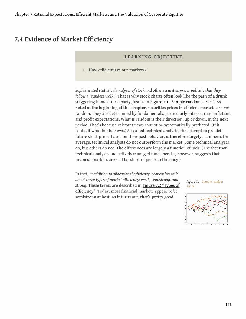
Figure 7.1 Sample randomseries
7.4 Evidence of Market Efficiency
LEARNING OBJECTIVE
1. How efficient are our markets?
Sophisticated statistical analyses of stock and other securities prices indicate that theyfollow a “random walk.” That is why stock charts often look like the path of a drunkstaggering home after a party, just as in Figure 7.1 "Sample random series". Asnoted at the beginning of this chapter, securities prices in efficient markets are notrandom. They are determined by fundamentals, particularly interest rate, inflation,and profit expectations. What is random is their direction, up or down, in the nextperiod. That’s because relevant news cannot be systematically predicted. (If itcould, it wouldn’t be news.) So-called technical analysis, the attempt to predictfuture stock prices based on their past behavior, is therefore largely a chimera. Onaverage, technical analysts do not outperform the market. Some technical analystsdo, but others do not. The differences are largely a function of luck. (The fact thattechnical analysts and actively managed funds persist, however, suggests thatfinancial markets are still far short of perfect efficiency.)
In fact, in addition to allocational efficiency, economists talkabout three types of market efficiency: weak, semistrong, andstrong. These terms are described in Figure 7.2 "Types ofefficiency". Today, most financial markets appear to besemistrong at best. As it turns out, that’s pretty good.
Chapter 7 Rational Expectations, Efficient Markets, and the Valuation of Corporate Equities
138
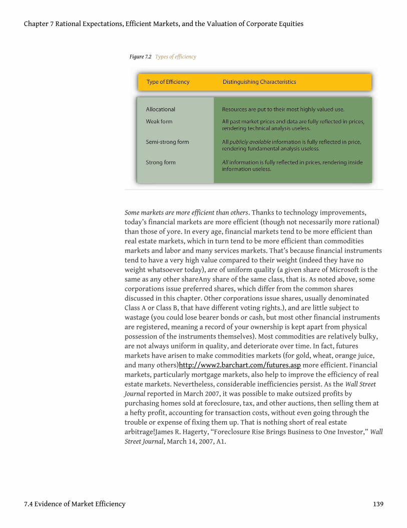
Figure 7.2 Types of efficiency
Some markets are more efficient than others. Thanks to technology improvements,today’s financial markets are more efficient (though not necessarily more rational)than those of yore. In every age, financial markets tend to be more efficient thanreal estate markets, which in turn tend to be more efficient than commoditiesmarkets and labor and many services markets. That’s because financial instrumentstend to have a very high value compared to their weight (indeed they have noweight whatsoever today), are of uniform quality (a given share of Microsoft is thesame as any other shareAny share of the same class, that is. As noted above, somecorporations issue preferred shares, which differ from the common sharesdiscussed in this chapter. Other corporations issue shares, usually denominatedClass A or Class B, that have different voting rights.), and are little subject towastage (you could lose bearer bonds or cash, but most other financial instrumentsare registered, meaning a record of your ownership is kept apart from physicalpossession of the instruments themselves). Most commodities are relatively bulky,are not always uniform in quality, and deteriorate over time. In fact, futuresmarkets have arisen to make commodities markets (for gold, wheat, orange juice,and many others)http://www2.barchart.com/futures.asp more efficient. Financialmarkets, particularly mortgage markets, also help to improve the efficiency of realestate markets. Nevertheless, considerable inefficiencies persist. As the Wall StreetJournal reported in March 2007, it was possible to make outsized profits bypurchasing homes sold at foreclosure, tax, and other auctions, then selling them ata hefty profit, accounting for transaction costs, without even going through thetrouble or expense of fixing them up. That is nothing short of real estatearbitrage!James R. Hagerty, “Foreclosure Rise Brings Business to One Investor,” WallStreet Journal, March 14, 2007, A1.
Chapter 7 Rational Expectations, Efficient Markets, and the Valuation of Corporate Equities
7.4 Evidence of Market Efficiency 139
Labor and services markets are the least efficient of all. People won’t or can’t move totheir highest valued uses; they adapt very slowly to technology changes; andmyriad regulations, some imposed by government and others by labor unions, limittheir flexibility on the job. Some improvements have been made in recent yearsthanks to global outsourcing, but it is clear that the number of unexploited profitopportunities in labor markets far exceeds those in the financial markets. Finally,markets for education,http://www.forbes.com/columnists/2005/12/29/higher-education-partnerships-cx_rw_1230college.htmlhealthcare,http://www.amazon.com/Fubarnomics-Lighthearted-Serious-Americas-Economic/dp/1616141913/ref=ntt_at_ep_dpi_3 http://www.amazon.com/Broken-Buildings-Busted-Budgets-Trillion-Dollar/dp/0226472671/ref=sr_1_1/002-2618567-2654432?ie=UTF8&s=books&qid=1177704792&sr=1-1 are also highlyinefficient, probably due to high levels of asymmetric information, a subjectaddressed in more detail below and in Chapter 8 "Financial Structure, TransactionCosts, and Asymmetric Information".
Chapter 7 Rational Expectations, Efficient Markets, and the Valuation of Corporate Equities
7.4 Evidence of Market Efficiency 140
Stop and Think Box
A friend urges you to subscribe to a certain reputable investment report.Should you buy? Another friend brags about the huge returns she has made bybuying and selling stocks frequently. Should you emulate her tradingstrategies?
Buying an investment report makes more sense than following the unsolicitedhot stock tip discussed above, but it still may not be a good idea. Manylegitimate companies try to sell information and advice to investors. The valueof that information and advice, however, may be limited. As we’ll learn inChapter 8 "Financial Structure, Transaction Costs, and AsymmetricInformation", the information may be tainted by conflicts of interest. Even ifthe research is unbiased and good, by the time the newsletter reaches you, evenif it is electronic, the market has probably already priced the information, sothere will be no above-market profit opportunities remaining to exploit. In fact,only one investment advice newsletter, Value Line Survey (VLS), has consistentlyprovided advice that leads to abnormally high risk-adjusted returns. It isn’tclear if VLS has deeper insights into the market, if it has simply gotten lucky, orif its mystique has made its predictions a self-fulfilling prophecy: investorsbelieve that it picks super stocks, so they buy its recommendations, drivingprices up, just as it predicted! The three explanations are not, in fact, mutuallyexclusive. Luck and skill may have created the mystique underlying VLS’scontinued success.
As far as emulating your friend’s trading strategies, you should investigate thematter more thoroughly first. For starters, people tend to brag about theirgains and forget about their losses. (My [Wright’s] father, who liked to bet theponies, was infamous for this. He’d get us excited by telling us he won $1,000 atthe track that day. When we asked why we were eating squirrels for dinneragain, he’d finally give in and admit that he also lost $1,200.) Even if your friendis genuinely successful at picking stocks, she is likely just getting lucky. Herluck could turn just as your money gets in the game. To the extent that marketsare efficient, investors are better off choosing the level of risk they arecomfortable with and earning the market return. That usually entails buyingand holding a diverse portfolio via an indexed mutual fund, which minimizestaxes and brokerage fees, both of which can add up. Long-term index investorsalso waste less time tracking stocks and worrying about market gyrations.
Chapter 7 Rational Expectations, Efficient Markets, and the Valuation of Corporate Equities
7.4 Evidence of Market Efficiency 141
As noted above, none of this should be taken to mean that financial markets areperfectly efficient. Researchers have uncovered certain anomalies, situations where it is orwas possible to outperform the market, holding risk and liquidity constant. I say wasbecause exposing an anomaly will often induce investors to exploit it until it iseliminated. One such anomaly was the so-called January Effect, a predictable rise instock prices that for many years occurred each January until its existence wasrecognized and publicized. Similarly, stock prices in the past tended to displaymean reversion. In other words, stocks with low returns in one period tended tohave high returns in the next, and vice versa. The phenomenon appears to havedisappeared, however, with the advent of trading strategies like the Dogs of theDow, where investors buy beaten-down stocks in the knowledge that they can onlygo up (though a few will go to zero and stay there).http://www.dogsofthedow.com/
Other anomalies, though, appear to persist. The prices of many financial securities,including stocks, tend to overshoot when there is unexpected bad news. After ahuge initial drop, the price often meanders back upward over a period of severalweeks. This suggests that investors should buy soon after bad news hits, then sell ata higher price a few weeks later. Sometimes, prices seem to adjust only slowly tonews, even highly specific announcements about corporate profit expectations.That suggests that investors could earn above-market returns by buyingimmediately on good news and selling after a few weeks when the price catches upto the news.
Some anomalies may be due to deficiencies in our understanding of risk and liquidity ratherthan market inefficiency. One of these is the small-firm effect. Returns on smallercompanies, apparently holding risk and liquidity constant, are abnormally large.Why then don’t investors flock to such companies, driving their stock prices upuntil the outsized returns disappear? Some suspect that the companies are riskier,or at least appear riskier to investors, than researchers believe. Others believe theroot issues are asymmetric information, the fact that the quality and quantity ofinformation about smaller firms is inferior to that of larger ones, an inaccuratemeasurement of liquidity. Similarly, some researchers believe that stock prices aremore volatile than they should be given changes in underlying fundamentals. Thatfinding too might stem from the fact that researchers aren’t as prescient as themarket.
The most important example of financial market inefficiencies are so-called asset bubbles ormanias. Periodically, market prices soar far beyond what the fundamentals suggestthey should. During stock market manias, like the dot-com bubble of the late 1990s,investors apparently popped sanguine values for g into models like the Gordongrowth model or, given the large run-up in prices, large P1 values into the one-
period valuation model. In any event, starting in March 2000, the valuations formost of the shares were discovered to be too high, so share prices rapidly dropped.
Chapter 7 Rational Expectations, Efficient Markets, and the Valuation of Corporate Equities
7.4 Evidence of Market Efficiency 142
Bubbles are not necessarily irrational, but they are certainly inefficient to the extent thatthey lead to the misallocation of resources when prices are rising and unexploited profitopportunities when prices head south.
Asset bubbles are very common affairs. Since the tech bubble burst, we’ve alreadyexperienced another, in housing and home mortgages. Recurrent investor euphoriamay be rooted in the deepest recesses of the human mind. Whether we evolvedfrom the great apes or were created by some Divine Being, one thing is clear: ourbrains are pretty scrambled, especially when it comes to probabilities and percentages. Forexample, a recent studyMarkus Glaser, Thomas Langer, Jens Reynders, and MartinWeber, “Framing Effects in Stock Market Forecasts: The Differences Between Askingfor Prices and Asking for Returns,” Review of Finance (2007) 11:325–357. published inReview of Finance showed that investors, even sophisticated ones, expect less changein future stock prices when asked to state their forecasts in currency (so manydollars or euros per share) than when asked to state them as returns (a percentagegain or loss).This is a new example of the well-known framing effect. Predict thefuture stock price of a stock that goes from $35 to $37 to $39 to $41 to $43 to $45.Now predict the future stock price of a stock whose returns are +$2, +$2, +$2, +$2,+$2, and +$2. If you are like most people, your answer to the first will be less than$45 but your answer to the second will be +$2 even though both series provideprecisely the same information. In other words, the way a problem is set up orframed influences the way people respond to it.
Behavioral finance16 uses insights from evolutionary psychology, anthropology,sociology, the neurosciences, and psychology to try to unravel how the humanbrain functions in areas related to finance.http://www.behaviouralfinance.net/ Forexample, many people are averse to short selling17, selling (or borrowing and thenselling) a stock that appears overvalued with the expectation of buying it back laterat a lower price. (Short sellers profit by owning more shares of the stock, or thesame number of shares and a sum of cash, depending on how they go about it.) Adearth of short selling may allow stock prices to spiral too high, leading to assetbubbles. Another human foible is that we tend to be overly confident in our ownjudgments. Many actually believe that they are smarter than the markets in whichthey trade! (As noted above, many researchers appear to fall into the same trap.)People also tend to herd. They will, like the common misconception aboutlemmings, run with the crowd, seemingly oblivious to the cliff looming just ahead.
Finally, as noted above, another source of inefficiency in financial (andnonfinancial) markets is asymmetric information, when one party to a transactionhas better information than the other. Usually, the asymmetry arises due to insideinformation as when the seller, for instance, knows the company is weak but thebuyer does not. Regulators try to reduce information asymmetries by outlawingoutright fraud and by encouraging timely and full disclosure of pertinent
16. A new interdisciplinary subjectmatter that tries to understandthe limits of human rationality,especially as it applies tofinancial markets.
17. Selling a stock at a high priceand buying it back later at alower price. It is the logicalequivalent of buying low andselling high, but manyinvestors don’t attempt it.
Chapter 7 Rational Expectations, Efficient Markets, and the Valuation of Corporate Equities
7.4 Evidence of Market Efficiency 143

information to the public. In short, they try to promote what economists calltransparency18. Some markets, however, remain quite opaque.http://ftp.sec.gov/news/speech/spch010606css.htm
In short, our financial markets appear to be semistrong form efficient. Greatertransparency and more fervent attempts to overcome the natural limitations ofhuman rationality would help to move the markets closer to strong form efficiency.
KEY TAKEAWAYS
• Beyond allocational efficiency, markets may be classed as weak,semistrong, or strong form efficient.
• If the market is weak form efficient, technical analysis is useless becausesecurities prices already reflect past prices.
• If the market is semistrong form efficient, fundamental analysis is alsouseless because prices reflect all publicly available information.
• If the market is strong form efficient, inside information is useless toobecause prices reflect all information.
• Securities prices tend to track each other closely over time and in factusually display random walk behavior, moving up and downunpredictably.
• Neither technical analysis nor fundamental analysis outperforms themarket on average, but inside information apparently does, so mostfinancial markets today are at best semistrong form efficient.
• Although more efficient than commodities, labor, and services markets,financial markets are not completely efficient.
• Various anomalies, like the January and small-firm effects, marketoverreaction and volatility, mean reversion, and asset bubbles, suggestthat securities markets sometimes yield outsized gains to the quick andthe smart, people who overcome the mushy, often illogical brains allhumans are apparently born with. But the quest is a never-ending one;no strategy works for long.
18. In general, the opposite ofopacity. In this context,transparency means arelatively low degree ofasymmetric information.
Chapter 7 Rational Expectations, Efficient Markets, and the Valuation of Corporate Equities
7.4 Evidence of Market Efficiency 144
7.5 Suggested Reading
Bernstein, Peter. Against the Gods: The Remarkable Story of Risk. Hoboken, NJ: JohnWiley and Sons, 1998.
Burnham, Terry. Mean Markets and Lizard Brains: How to Profit from the New Science ofIrrationality. Hoboken, NJ: John Wiley and Sons, 2008.
English, James. Applied Equity Analysis: Stock Valuation Techniques for Wall StreetProfessionals. New York: McGraw-Hill, 2001.
Mackay, Charles, and Joseph de la Vega. Extraordinary Popular Delusions and theMadness of Crowds and Confusion de Confusiones. Hoboken, NJ: John Wiley and Sons,1995.
Malkiel, Burton. A Random Walk Down Wall Street: The Time-Tested Strategy forSuccessful Investing, 9th ed. New York: W. W. Norton, 2007.
Chapter 7 Rational Expectations, Efficient Markets, and the Valuation of Corporate Equities
145
Chapter 8
Financial Structure, Transaction Costs, and AsymmetricInformation
CHAPTER OBJECTIVES
By the end of this chapter, students should be able to:
1. Describe how nonfinancial companies meet their external financingneeds.
2. Explain why bonds play a relatively large role in the external financingof U.S. companies.
3. Explain why most external finance is channeled through financialintermediaries.
4. Define transaction costs and explain their importance.5. Define and describe asymmetric information and its importance.6. Define and explain adverse selection, moral hazard, and agency
problems.7. Explain why the financial system is heavily regulated.
146
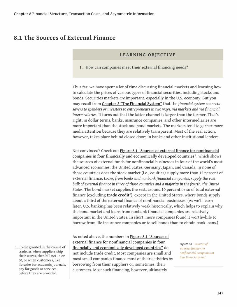
Figure 8.1 Sources ofexternal finance fornonfinancial companies infour financially and
8.1 The Sources of External Finance
LEARNING OBJECTIVE
1. How can companies meet their external financing needs?
Thus far, we have spent a lot of time discussing financial markets and learning howto calculate the prices of various types of financial securities, including stocks andbonds. Securities markets are important, especially in the U.S. economy. But youmay recall from Chapter 2 "The Financial System" that the financial system connectssavers to spenders or investors to entrepreneurs in two ways, via markets and via financialintermediaries. It turns out that the latter channel is larger than the former. That’sright, in dollar terms, banks, insurance companies, and other intermediaries aremore important than the stock and bond markets. The markets tend to garner moremedia attention because they are relatively transparent. Most of the real action,however, takes place behind closed doors in banks and other institutional lenders.
Not convinced? Check out Figure 8.1 "Sources of external finance for nonfinancialcompanies in four financially and economically developed countries", which showsthe sources of external funds for nonfinancial businesses in four of the world’s mostadvanced economies: the United States, Germany, Japan, and Canada. In none ofthose countries does the stock market (i.e., equities) supply more than 12 percent ofexternal finance. Loans, from banks and nonbank financial companies, supply the vastbulk of external finance in three of those countries and a majority in the fourth, the UnitedStates. The bond market supplies the rest, around 10 percent or so of total externalfinance (excluding trade credit1), except in the United States, where bonds supplyabout a third of the external finance of nonfinancial businesses. (As we’ll learnlater, U.S. banking has been relatively weak historically, which helps to explain whythe bond market and loans from nonbank financial companies are relativelyimportant in the United States. In short, more companies found it worthwhile toborrow from life insurance companies or to sell bonds than to obtain bank loans.)
As noted above, the numbers in Figure 8.1 "Sources ofexternal finance for nonfinancial companies in fourfinancially and economically developed countries" donot include trade credit. Most companies are small andmost small companies finance most of their activities byborrowing from their suppliers or, sometimes, theircustomers. Most such financing, however, ultimately
1. Credit granted in the course oftrade, as when suppliers shiptheir wares, then bill net 15 or30, or when customers, likelibraries for academic journals,pay for goods or servicesbefore they are provided.
Chapter 8 Financial Structure, Transaction Costs, and Asymmetric Information
147
economically developedcountries
comes from loans, bonds, or stock. In other words,companies that extend trade credit act, in a sense, as nonbankintermediaries, channeling equity, bonds, and loans tosmall companies. This makes sense because suppliersusually know more about small companies than banksor individual investors do. And information, we’ll see, iskey.
Also note that the equity figures are somewhatmisleading given that, once sold, a share provides financing forever, or at least untilthe company folds or buys it back. The figures above do not account for that, so a$1,000 year-long bank loan renewed each year for 20 years would count as $20,000of bank loans, while the sale of $1,000 of equities would count only as $1,000.Despite that bias in the methodology, it is clear that most external finance does not, infact, come from the sale of stocks or bonds. Moreover, in less economically andfinancially developed countries, an even higher percentage of external financingcomes to nonfinancial companies via intermediaries rather than markets.
What explains the facts highlighted in Figure 8.1 "Sources of external finance fornonfinancial companies in four financially and economically developed countries"?Why are bank and other loans more important sources of external finance thanstocks and bonds? Why does indirect finance, via intermediaries, trump directfinance, via markets? For that matter, why are most of those loans collateralized2?Why are loan contracts so complex? Why are only the largest companies able toraise funds directly by selling stocks and bonds? Finally, why are financial systemsworldwide one of the most heavily regulated economic sectors?
Those questions can be answered in three ways: transaction costs, asymmetricinformation, and the free-rider problem. Explaining what those three terms mean,however, will take a little doing.
2. Pledge some asset, like land orfinancial securities, for therepayment of a loan.
Chapter 8 Financial Structure, Transaction Costs, and Asymmetric Information
8.1 The Sources of External Finance 148
KEY TAKEAWAYS
• To meet their external financing needs, companies can sell equity(stock) and commercial paper and longer-term bonds and they canobtain loans from banks and nonbank financial institutions.
• They can also obtain trade credit from suppliers and customers, butmost of those funds ultimately come from loans, bonds, or equity.
• Most external financing comes from loans, with bonds and equities adistant second, except in the United States, where bonds provide about athird of external financing for nonfinancial companies.
• Bonds play a relatively larger role in the external financing of U.S.companies because the U.S. banking system has been weak historically.That weakness induced companies to obtain more loans from nonbankfinancial institutions like life insurance companies and also to issuemore bonds.
Chapter 8 Financial Structure, Transaction Costs, and Asymmetric Information
8.1 The Sources of External Finance 149
8.2 Transaction Costs, Asymmetric Information, and the Free-RiderProblem
LEARNING OBJECTIVE
1. Why is most external finance channeled through financialintermediaries?
Minimum efficient scale3 in finance is larger than most individuals can invest.Somebody with $100, $1,000, $10,000, even $100,000 to invest would have a hardtime making any profit at all, let alone the going risk-adjusted return. That isbecause most of his or her profits would be eaten up in transaction costs, brokerage fees, theopportunity cost of his or her time, and liquidity and diversification losses. Many types ofbonds come in $10,000 increments and so are out of the question for many smallinvestors. A single share of some companies, like Berkshire Hathaway, coststhousands or tens of thousands of dollars and so is also out ofreach.http://www.berkshirehathaway.com/ Most shares cost far less, buttransaction fees, even after the online trading revolution of the early 2000s, are stillquite high, especially if an investor were to try to diversify by buying only a fewshares of many companies. As discussed in Chapter 7 "Rational Expectations,Efficient Markets, and the Valuation of Corporate Equities", financial markets are soefficient that arbitrage opportunities are rare and fleeting. Those who make a livingengaging in arbitrage, like hedge fund D. E. Shaw, do so only through scaleeconomies. They need superfast (read “expensive”) computers and nerdy (read“expensive”) employees to operate custom (read “expensive”) programs on them.They also need to engage in large-scale transactions. You can’t profit making .001percent on a $1,000 trade, but you can on a $1,000,000,000 one.
What about making loans directly to entrepreneurs or other borrowers?Fuggeddaboutit! The time, trouble, and cash (e.g., for advertisements like that inFigure 8.2 "Need a loan?") it would take to find a suitable borrower would likelywipe out any profits from interest. The legal fees alone would swamp you! (It helpsif you can be your own lawyer, like John C. Knapp.) And, as we’ll learn below, makingloans isn’t all that easy. You’ll still occasionally see advertisements like those thatused to appear in the eighteenth century, but they are rare and might in fact beplaced by predators, people who are more interested in robbing you (or worse) thanlending to you. A small investor might be able to find a relative, co-religionist,colleague, or other acquaintance to lend to relatively cheaply. But how could theinvestor know if the borrower was the best one, given the interest rate charged?
3. The smallest a business can beand still remain efficient and/or profitable.
Chapter 8 Financial Structure, Transaction Costs, and Asymmetric Information
150

Figure 8.2 Need a loan?
From Early AmericanNewspapers, an Archive ofAmericana Collection, publishedby Readex (Readex.com), adivision of NewsBank, Inc.
What is the best rate, anyway? To answer those questions even haphazardly wouldcost relatively big bucks. And here is another hint: friends and relatives often thinkthat a “loan” is actually a “gift,” if you catch my “drift.”
A new type of banking, called peer-to-peer banking4,might reduce some of those transaction costs. In peer-to-peer banking, a financial facilitator, like Zopa.com orProsper.com, reduces transaction costs by electronicallymatching individual borrowers and lenders. Most peer-to-peer facilitators screen loan applicants in at least arudimentary fashion and also provide diversificationservices, distributing lenders’ funds to numerousborrowers to reduce the negative impact of anydefaults.For details, see “Options Grow for Investors toLend Online,” Wall Street Journal, July 18, 2007. Althoughthe infant industry is currently growing, the peer-to-peerconcept is still unproven and there are powerful reasons todoubt its success. Even if the concept succeeds (and itmight given its Thomas Friedman–The World IsFlatishnesshttp://en.wikipedia.org/wiki/The_World_is_Flat), it will only reinforce the pointmade here about the inability of most individuals toinvest profitably without help.
Financial intermediaries clearly can provide such help. They have been doing so forat least a millennium (yep, a thousand years, maybe more). One key to their success istheir ability to achieve minimum efficient scale. Banks, insurers, and otherintermediaries pool the resources of many investors. That allows them to diversifycheaply because instead of buying 10 shares of XYZ’s $10 stock and paying $7 forthe privilege (7/100 = .07) they can buy 1,000,000 shares for a brokerage fee ofmaybe $1,000 ($1,000/1,000,000 = .001). In addition, financial intermediaries do nothave to sell assets as frequently as individuals (ceteris paribus, of course) becausethey can usually make payments out of inflows like deposits or premium payments.Their cash flow, in other words, reduces their liquidity costs. Individual investors,on the other hand, often find it necessary to sell assets (and incur the costsassociated therewith) to pay their bills.
As specialists, financial intermediaries are also experts at what they do. That does notmean that they are perfect—far from it, as we learned during the financial crisisthat began in 2007—but they are certainly more efficient at accepting deposits,making loans, or insuring risks than you or I will ever be (unless we work for afinancial intermediary, in which case we’ll likely become incredibly efficient in oneor at most a handful of functions). That expertise covers many areas, from database
4. In this new type of banking, afacilitator links lenders toborrowers, acting more like asecurities broker than a bank.
Chapter 8 Financial Structure, Transaction Costs, and Asymmetric Information
8.2 Transaction Costs, Asymmetric Information, and the Free-Rider Problem 151
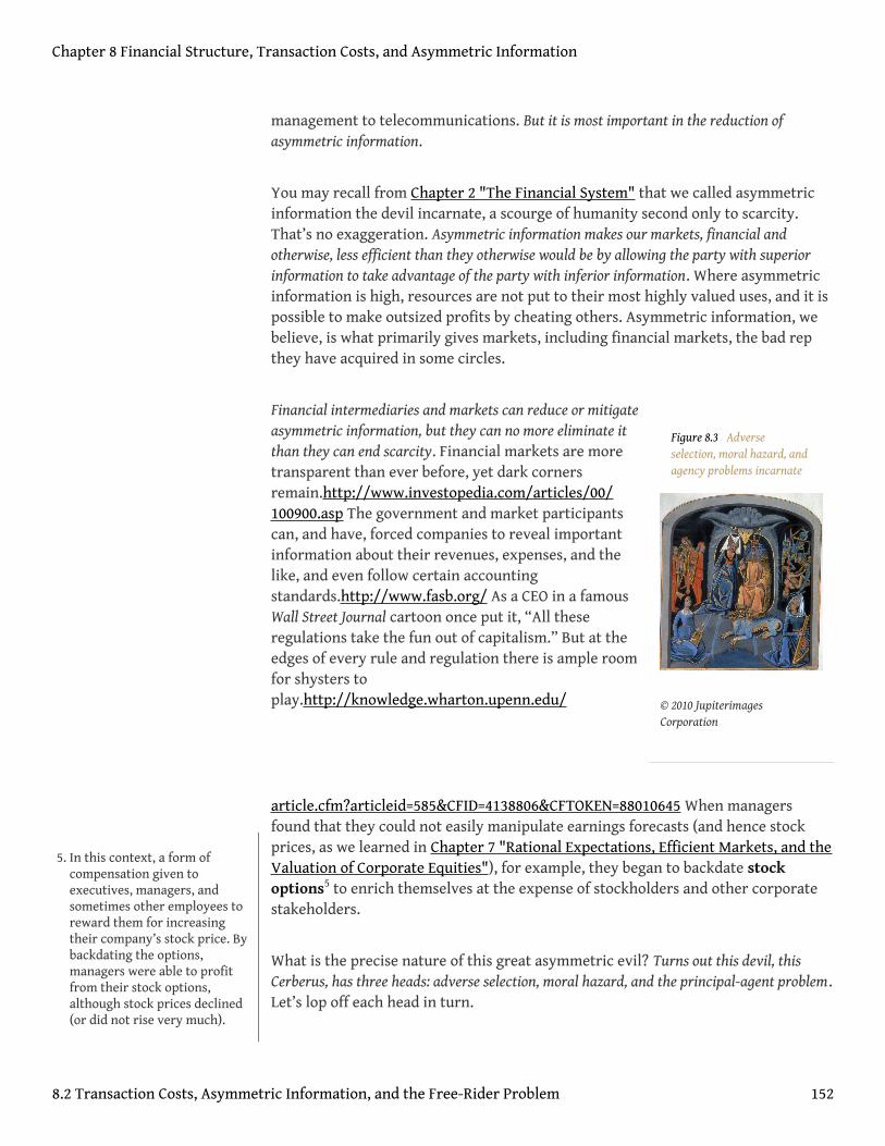
Figure 8.3 Adverseselection, moral hazard, andagency problems incarnate
© 2010 JupiterimagesCorporation
management to telecommunications. But it is most important in the reduction ofasymmetric information.
You may recall from Chapter 2 "The Financial System" that we called asymmetricinformation the devil incarnate, a scourge of humanity second only to scarcity.That’s no exaggeration. Asymmetric information makes our markets, financial andotherwise, less efficient than they otherwise would be by allowing the party with superiorinformation to take advantage of the party with inferior information. Where asymmetricinformation is high, resources are not put to their most highly valued uses, and it ispossible to make outsized profits by cheating others. Asymmetric information, webelieve, is what primarily gives markets, including financial markets, the bad repthey have acquired in some circles.
Financial intermediaries and markets can reduce or mitigateasymmetric information, but they can no more eliminate itthan they can end scarcity. Financial markets are moretransparent than ever before, yet dark cornersremain.http://www.investopedia.com/articles/00/100900.asp The government and market participantscan, and have, forced companies to reveal importantinformation about their revenues, expenses, and thelike, and even follow certain accountingstandards.http://www.fasb.org/ As a CEO in a famousWall Street Journal cartoon once put it, “All theseregulations take the fun out of capitalism.” But at theedges of every rule and regulation there is ample roomfor shysters toplay.http://knowledge.wharton.upenn.edu/
article.cfm?articleid=585&CFID=4138806&CFTOKEN=88010645 When managersfound that they could not easily manipulate earnings forecasts (and hence stockprices, as we learned in Chapter 7 "Rational Expectations, Efficient Markets, and theValuation of Corporate Equities"), for example, they began to backdate stockoptions5 to enrich themselves at the expense of stockholders and other corporatestakeholders.
What is the precise nature of this great asymmetric evil? Turns out this devil, thisCerberus, has three heads: adverse selection, moral hazard, and the principal-agent problem.Let’s lop off each head in turn.
5. In this context, a form ofcompensation given toexecutives, managers, andsometimes other employees toreward them for increasingtheir company’s stock price. Bybackdating the options,managers were able to profitfrom their stock options,although stock prices declined(or did not rise very much).
Chapter 8 Financial Structure, Transaction Costs, and Asymmetric Information
8.2 Transaction Costs, Asymmetric Information, and the Free-Rider Problem 152
KEY TAKEAWAYS
• Transaction costs, asymmetric information, and the free-rider problemexplain why most external finance is channeled through intermediaries.
• Most individuals do not control enough funds to invest profitably giventhe fact that fixed costs are high and variable costs are low in most areasof finance. In other words, it costs almost as much to buy 10 shares as itdoes to buy 10,000.
• Also, individuals do not engage in enough transactions to be proficientor expert at it.
• Financial intermediaries, by contrast, achieve minimum efficient scaleand become quite expert at what they do, though they remain far fromperfect.
• Transaction costs are any and all costs associated with completing anexchange.
• Transaction costs include, but are not limited to, broker commissions;dealer spreads; bank fees; legal fees; search, selection, and monitoringcosts; and the opportunity cost of time devoted to investment-relatedactivities.
• They are important because they detract from bottom-line profits,eliminating or greatly reducing them in the case of individuals and firmsthat have not achieved minimum efficient scale.
• Transaction costs are one reason why institutional intermediariesdominate external finance.
Chapter 8 Financial Structure, Transaction Costs, and Asymmetric Information
8.2 Transaction Costs, Asymmetric Information, and the Free-Rider Problem 153

8.3 Adverse Selection
LEARNING OBJECTIVE
1. What problems do asymmetric information and, more specifically,adverse selection cause and how can they be mitigated?
The classic case of adverse selection, the one that brought the phenomenon backClassicaleconomists like Adam Smith recognized adverse selection and asymmetricinformation more generally, but they did not label or stress the concepts.to theattention of economists in 1970, is the market for “lemons,” which is to say, breakdown-prone automobiles. The lemons story, with appropriate changes, applies toeverything from horses to bonds, to lemons (the fruit), to construction services.That is because the lemons story is a simple but powerful one. People who offerlemons for sale know that their cars stink. Most people looking to buy cars, though,can’t tell that a car is prone to breakdown. They might kick the tires, take it for ashort spin, look under the hood, etc., all without discovering the truth. The sellerhas superior information and indeed has an incentive to increase the asymmetry byputting a Band-Aid over any obvious problems. (He might, for example, warm thecar up thoroughly before showing it, put top-quality gasoline in the tank, clean upthe oil spots in the driveway, and so forth.) He may even explain that the car wasowned by his poor deceased grandmother, who used it only to drive to church onSundays (for services) and Wednesdays (for bingo), and that she took meticulouscare of it. The hapless buyer, the story goes, offers the average price for used cars ofthe particular make, model, year, and mileage for sale. The seller happily (and greedilyif you want to be moralistic about it) accepts. A day, week, month, or year later, the buyerslearns that he has overpaid, that the automobile he purchased is a lemon. He complains tohis relatives, friends, and neighbors, many of whom tell similar horror stories. Aconsensus emerges that all used cars are lemons.
Of course, some used cars are actually “peaches,” very reliable means of personaltransportation. The problem is that owners of peaches can’t credibly inform buyersof the car’s quality. Oh, she can say, truthfully, that the car was owned by her poordeceased grandmother who used it only to drive to church on Sundays (for services)and Wednesdays (for bingo) and that she took meticulous care of it. But that soundsa lot like what the owner of the lemon says too. (In fact, we just copied and pasted itfrom above!) So the asymmetric information remains and the hapless buyer offersthe average price for used cars of the particular make, model, year, and mileage forsale. (Another copy and paste job!) But this time the seller, instead of accepting the offer,gets offended and storms off (or at least declines). So the buyer’s relatives, friends, and
Chapter 8 Financial Structure, Transaction Costs, and Asymmetric Information
154
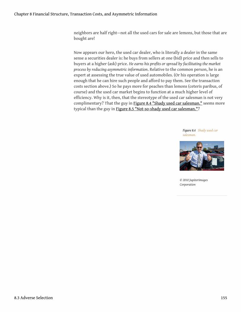
Figure 8.4 Shady used carsalesman.
© 2010 JupiterimagesCorporation
neighbors are half right—not all the used cars for sale are lemons, but those that arebought are!
Now appears our hero, the used car dealer, who is literally a dealer in the samesense a securities dealer is: he buys from sellers at one (bid) price and then sells tobuyers at a higher (ask) price. He earns his profits or spread by facilitating the marketprocess by reducing asymmetric information. Relative to the common person, he is anexpert at assessing the true value of used automobiles. (Or his operation is largeenough that he can hire such people and afford to pay them. See the transactioncosts section above.) So he pays more for peaches than lemons (ceteris paribus, ofcourse) and the used car market begins to function at a much higher level ofefficiency. Why is it, then, that the stereotype of the used car salesman is not verycomplimentary? That the guy in Figure 8.4 "Shady used car salesman." seems moretypical than the guy in Figure 8.5 "Not-so-shady used car salesman."?
Chapter 8 Financial Structure, Transaction Costs, and Asymmetric Information
8.3 Adverse Selection 155
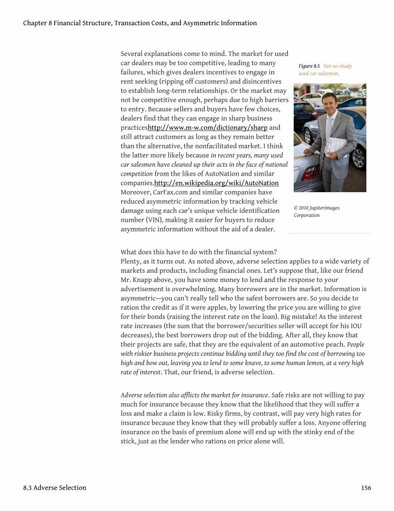
Figure 8.5 Not-so-shadyused car salesman.
© 2010 JupiterimagesCorporation
Several explanations come to mind. The market for usedcar dealers may be too competitive, leading to manyfailures, which gives dealers incentives to engage inrent seeking (ripping off customers) and disincentivesto establish long-term relationships. Or the market maynot be competitive enough, perhaps due to high barriersto entry. Because sellers and buyers have few choices,dealers find that they can engage in sharp businesspracticeshttp://www.m-w.com/dictionary/sharp andstill attract customers as long as they remain betterthan the alternative, the nonfacilitated market. I thinkthe latter more likely because in recent years, many usedcar salesmen have cleaned up their acts in the face of nationalcompetition from the likes of AutoNation and similarcompanies.http://en.wikipedia.org/wiki/AutoNationMoreover, CarFax.com and similar companies havereduced asymmetric information by tracking vehicledamage using each car’s unique vehicle identificationnumber (VIN), making it easier for buyers to reduceasymmetric information without the aid of a dealer.
What does this have to do with the financial system?Plenty, as it turns out. As noted above, adverse selection applies to a wide variety ofmarkets and products, including financial ones. Let’s suppose that, like our friendMr. Knapp above, you have some money to lend and the response to youradvertisement is overwhelming. Many borrowers are in the market. Information isasymmetric—you can’t really tell who the safest borrowers are. So you decide toration the credit as if it were apples, by lowering the price you are willing to givefor their bonds (raising the interest rate on the loan). Big mistake! As the interestrate increases (the sum that the borrower/securities seller will accept for his IOUdecreases), the best borrowers drop out of the bidding. After all, they know thattheir projects are safe, that they are the equivalent of an automotive peach. Peoplewith riskier business projects continue bidding until they too find the cost of borrowing toohigh and bow out, leaving you to lend to some knave, to some human lemon, at a very highrate of interest. That, our friend, is adverse selection.
Adverse selection also afflicts the market for insurance. Safe risks are not willing to paymuch for insurance because they know that the likelihood that they will suffer aloss and make a claim is low. Risky firms, by contrast, will pay very high rates forinsurance because they know that they will probably suffer a loss. Anyone offeringinsurance on the basis of premium alone will end up with the stinky end of thestick, just as the lender who rations on price alone will.
Chapter 8 Financial Structure, Transaction Costs, and Asymmetric Information
8.3 Adverse Selection 156
Like used car dealers, financial facilitators and intermediaries seek to profit by reducingadverse selection. They do so by specializing in discerning good from bad credit andinsurance risks. Their main weapon here is called screening and it’s what all those formsand questions are about when you apply for a loan or insurance policy. Potential lenderswant to know if you pay your bills on time, if your income minus expenses is largeand stable enough to service the loan, if you have any collateral that might protectthem from loss, and the like. Potential insurers want to know if you have filed manyinsurance claims in the past because that may indicate that you are clumsy; notvery careful with your possessions; or worse, a shyster who makes a living filinginsurance claims. They also want to know more about the insured property so theydon’t insure it for too much, a sure inducement to start a fire or cause an accident.They also need to figure out how much risk is involved, how likely a certain type ofcar is to be totaled if involved in an accident,http://www.edmunds.com/ownership/safety/articles/43804/article.html the probability of a wood-framehouse burning to the ground in a given area,http://www.usfa.dhs.gov/statistics/estimates/index.shtm the chance of a Rolex watch being stolen, and so forth.
Stop and Think Box
Credit-protection insurance policies promise to make payments to people whofind themselves unemployed or incapacitated. Whenever solicited to buy suchinsurance, I (Wright) always ask how the insurer overcomes adverse selectionbecause there are never any applications or premium schedules, just one fixedrate. Why do I care?
I care because I’m a peach of a person. I know that if I lived a more dangerouslifestyle or was employed in a more volatile industry that I’d snap the policyright up. Given my current situation, however, I don’t think it very likely that Iwill become unemployed or incapacitated, so I don’t feel much urgency to buysuch a policy at the same rate as some guy or gal who’s about to go skydivinginstead of going to work. I don’t want to subsidize them or to deal with acompany that doesn’t know the first thing about insurance.
Financial intermediaries are not perfect screeners. They often make mistakes. Insurers likeState Farm, for example, underestimated the likelihood of a massive storm likeKatrina striking the Gulf Coast. And subprime mortgage lenders, companies thatlend to risky borrowers on the collateral of their homes, grossly miscalculated thelikelihood that their borrowers would default. Competition between lenders andinsurers induces them to lower their screening standards to make the sale. (In a
Chapter 8 Financial Structure, Transaction Costs, and Asymmetric Information
8.3 Adverse Selection 157
famous cartoon in the Wall Street Journal, a clearly nonplussed father asks aconcerned mom how their son’s imaginary friend got preapproved for a creditcard.) At some point, though, adverse selection always rears its ugly head, forcinglenders and insurance providers to improve their screening procedures and tightentheir standards once again. And, on average, they do much better than you or Iacting alone could do.
Another way of reducing adverse selection is the private production and sale of information.Companies like Standard and Poor’s, Bests, Duff and Phelps, Fitch’s, and Moody’sused to compile and analyze data on companies, rate the riskiness of their bonds,and then sell that information to investors in huge books. The free-rider problem6,though, killed off that business model. Specifically, the advent of cheapphotocopying induced people to buy the books, photocopy them, and sell them at afraction of the price that the bond-rating agencies could charge. (The free ridershad to pay only the variable costs of publication; the rating agencies had to pay thelarge fixed costs of compiling and analyzing the data.) So in the mid-1970s, thebond-rating agencies began to give their ratings away to investors and insteadcharged bond issuers for the privilege of being rated. The new model greatlydecreased the effectiveness of the ratings because the new arrangement quickly ledto rating inflation similar to grade inflation. (Pleasure flows with the cash. Insteadof pleasing investors, the agencies started to please the issuers.) After every majorfinancial crisis, including the subprime mortgage mess of 2007, academics andformer government regulators lambaste credit-rating agencies for their poorperformance relative to markets and point out the incentive flaws built into theirbusiness model. Thus far, little has changed, but encrypted databases might allow areturn to the investor-pay model. But then another form of free riding would ariseas investors who did not subscribe to the database would observe and mimic thetrades of those investors known to have subscriptions. Due to the free-rider probleminherent in markets, banks and other financial intermediaries have incentives to createprivate information about borrowers and people who are insured. This helps to explain whythey trump bond and stock markets.
Governments can no more legislate away adverse selection than they can end scarcity bydecree. They can, however, give markets and intermediaries a helping hand. In the UnitedStates, for example, the Securities and Exchange Commission (SEC) tries to ensurethat corporations provide market participants with accurate and timelyinformation about themselves, reducing the information asymmetry betweenthemselves and potential bond- and stockholders.http://www.sec.gov/ Like sellersof lemons, however, bad companies often outfox the SEC (and similar regulators inother countries) and investors, especially when said investors place too muchconfidence in government regulators. In 2001, for example, a high-flying energytrading company named Enron suddenly encountered insurmountable financialdifficulties and was forced to file for bankruptcy, the largest in American history at
6. Trying to hop a ride withoutpaying for it. More technically,it is any behavior where aparty takes more than his orher fair share of the benefits,or does not pay his or her fairshare of the costs, of someactivity.
Chapter 8 Financial Structure, Transaction Costs, and Asymmetric Information
8.3 Adverse Selection 158
that time. Few saw Enron’s implosion coming because the company hid its debt andlosses in a maze of offshore shell companies and other accounting smokescreens.Some dumbfounded investors hadn’t bothered watching the energy giant becausethey believed the government was doing it for them. It wasn’t.
KEY TAKEAWAYS
• Asymmetric information decreases the efficiency of financial markets,thereby reducing the flow of funds to entrepreneurs and injuring thereal economy.
• Adverse selection is precontractual asymmetric information.• It can be mitigated by screening out high-risk members of the applicant
pool.• Financial market facilitators can also become expert specialists and
attain minimum efficient scale, but financial markets are hampered bythe free-rider problem.
• In short, few firms find it profitable to produce information because it iseasy for others to copy and profit from it. Banks and otherintermediaries, by contrast, create proprietary information about theirborrowers and people they insure.
Chapter 8 Financial Structure, Transaction Costs, and Asymmetric Information
8.3 Adverse Selection 159
8.4 Moral Hazard
LEARNING OBJECTIVE
1. What is moral hazard and how can it be mitigated?
Adverse selection is precontractual asymmetric information. Moral hazard ispostcontractual asymmetric information. It occurs whenever a borrower or insuredentity (an approved borrower or policyholder, not a mere applicant) engages inbehaviors that are not in the best interest of the lender or insurer. If a borroweruses a bank loan to buy lottery tickets instead of Treasuries, as agreed upon withthe lender, that’s moral hazard. If an insured person leaves the door of his or herhome or car unlocked or lets candles burn all night unattended, that’s moralhazard. It’s also moral hazard if a borrower fails to repay a loan when he has thewherewithal to do so, or if an insured driver fakes an accident.
We call such behavior moral hazard because it was long thought to indicate a lack of moralsor character and in a sense it does. But thinking about the problem in those terms does nothelp to mitigate it. We all have a price. How high that price is can’t be easilydetermined and may indeed change, but offered enough money, every human being(except maybe Gandhi, prophets, and saints) will engage in immoral activities forpersonal gain if given the chance. It’s tempting indeed to put other people’s money atrisk. As we’ve learned, the more risk, the more reward. Why not borrow money toput to risk? If the rewards come, the principal and interest are easily repaid. If therewards don’t come, the borrower defaults and suffers but little. Back in the day, asthey say, borrowers who didn’t repay their loans were thrown into jail until theypaid up. Three problems eventually ended that practice. First, it is difficult to earnmoney to repay the loan when you’re imprisoned! (The original assumption wasthat the borrower had the money but wouldn’t cough it up.) Second, not everyonedefaults on a loan due to moral hazard. Bad luck, a soft economy, and/or poorexecution can turn the best business plan to mush. Third, lenders are almost asculpable as the borrowers for moral hazard if they don’t take steps to try tomitigate it. A locked door, an old adage goes, keeps an honest man honest. Don’ttempt people, in other words, and most won’t rob you. There are locks againstmoral hazard. They are not foolproof but they get the job done most of the time.
Chapter 8 Financial Structure, Transaction Costs, and Asymmetric Information
160
Stop and Think Box
Investment banks engage in many activities, two of which, research andunderwriting, have created conflicts of interest. The customers of ibanks’research activities, investors, want unbiased information. The customers ofibanks’ underwriting activities, bond issuers, want optimistic reports. A fewyears back, problems arose when the interests of bond issuers, who providedibanks with most of their profits, began to supersede the interests of investors.Specifically, ibank managers forced their research departments to avoidmaking negative or controversial comments about clients. The situation grewworse during the Internet stock mania of the late 1990s, when ibank researchanalysts like Jack Grubman (a Dickensian name but true!) of Citigroup (thenSalomon Smith Barney) made outrageous claims about the value of high-techcompanies. That in itself wasn’t evil because everyone makes mistakes. Whatraised hackles was that the private e-mails of those same analysts indicatedthat they thought the companies they were hyping were extremely weak. Andmost were. What sort of problem does this particular conflict of interestrepresent? How does it injure the economy? What can be done to rectify theproblem?
This is an example of asymmetric information and, more specifically, moralhazard. Investors contracted with the ibanks for unbiased investment researchbut instead received extremely biased advice that induced them to pay toomuch for securities, particularly the equities of weak tech companies. As aresult, the efficiency of our financial markets decreased as resources went tofirms that did not deserve them and could not put them to their most highlyvalued use. That, of course, injured economic growth. One way to solve thisproblem would be to allow ibanks to engage in securities underwriting orresearch, but not both. That would make ibanks less profitable, though, asdoing both creates economies of scope. (That’s why ibanks got into the businessof selling research in the first place.) Another solution is to create a “Chinesewall” within each ibank between their research and underwriting departments.This apparent reference to the Great Wall of China, which despite its grandeurwas repeatedly breached by “barbarian” invaders with help from insiders, alsobelies that strategy’s weakness.http://en.wikipedia.org/wiki/Great_Wall_of_China If the wall is so high that it is impenetrable, then theeconomies of scope are diminished to the vanishing point. If the wall is low orporous, then the conflict of interest can again arise. Rational expectations andtransparency could help here. Investors now know (or at least could/shouldknow) that ibanks can provide biased research reports and hence should
Chapter 8 Financial Structure, Transaction Costs, and Asymmetric Information
8.4 Moral Hazard 161
remain wary. Government regulations could help here by mandating thatibanks completely and accurately disclose their interests in the companies thatthey research and evaluate. That extra transparency would then allowinvestors to discount rosy prognostications that appear to be driven by ibanks’underwriting interests. The Global Legal Settlement of 2002, which wasbrokered by Eliot Spitzer (then New York State Attorney General and NewYork’s governor until he ran into a little moral hazard problem himself!), bansspinning, requires investment banks to sever the links between underwritingand research, and slapped a $1.4 billion fine on the ten largest ibanks.
The main weapon against moral hazard is monitoring, which is just a fancy term for payingattention! No matter how well they have screened (reduced adverse selection),lenders and insurers cannot contract and forget. They have to make sure that theircustomers do not use the superior information inherent in their situation to takeadvantage. Banks have a particularly easy and powerful way of doing this: watchingchecking accounts. Banks rarely provide cash loans because the temptation ofrunning off with the money, the moral hazard, would be too high. Instead, theycredit the amount of the loan to a checking account upon which the borrower candraw funds. (This procedure has a second positive feature for banks calledcompensatory balances. A loan for, say, $1 million does not leave the bank at oncebut does so only gradually. That raises the effective interest rate because theborrower pays interest on the total sum, not just that drawn out of the bank.) Thebank can then watch to ensure that the borrower is using the funds appropriately.Most loans contain restrictive covenants7, clauses that specify in great detail how theloan is to be used and how the borrower is to behave. If the borrower breaks one or morecovenants, the entire loan may fall due immediately. Covenants may require thatthe borrower obtain life insurance, that he or she keep collateral in good condition,or that various business ratios be kept within certainparameters.http://www.toolkit.cch.com/text/P06_7100.asp Often, loans willcontain covenants requiring borrowers to provide lenders with various types ofinformation, including audited financial reports, thus minimizing the lender’smonitoring costs.
Another powerful way of reducing moral hazard is to align incentives. That can be done bymaking sure the borrower or insured has some skin in thegame,http://www.answers.com/topic/skin-in-the-game that he, she, or it willsuffer if a loan goes bad or a loss is incurred. That will induce the borrower orinsured to behave in the lender’s or insurer’s best interest. Collateral, propertypledged for the repayment of a loan, is a good way to reduce moral hazard. Borrowersdon’t take kindly to losing, say, their homes. Also, the more equity they have—in
7. Clauses in loan contracts thatrestrict the uses to whichborrowed funds can be put andotherwise direct borrowerbehavior.
Chapter 8 Financial Structure, Transaction Costs, and Asymmetric Information
8.4 Moral Hazard 162
their home or business or investment portfolio—the harder they will fight to keepfrom losing it. Some will still default, but not purposely. In other words, the higherone’s net worth (market value of assets minus market value of liabilities), the lesslikely one is to default, which could trigger bankruptcy proceedings that wouldreduce or even wipe out the borrower’s net worth. This is why, by the way, it issometimes alleged that you have to have money to borrow money. That isn’tliterally true, of course. What is true is that owning assets free and clear of debtmakes it much easier to borrow.
Similarly, insurers long ago learned that they should insure only a part of the valueof a ship, car, home, or life. That is why they insist on deductibles or co-insurance. If youwill lose nothing if you total your car, you might attempt that late-night trip on icyroads or sign up for a demolition derby. If an accident will cost you $500(deductible) or 20 percent of the costs of the damage (co-insurance), you will thinktwice or thrice before doing something risky with your car.
When it comes to reducing moral hazard, financial intermediaries have advantagesover individuals. Monitoring is not cheap. Indeed, economists sometimes refer to it as“costly state verification.” Economies of scale give intermediaries an upper hand.Monitoring is also not easy, so specialization and expertise also render financialintermediaries more efficient than individuals at reducing moral hazard. If nothingelse, financial intermediaries can afford to hire the best legal talent to frighten thedevil out of would-be scammers. Borrowers can no longer be imprisoned fordefaulting, but they can go to prison for fraud. Statutes against fraud are one waythat the government helps to chop at the second head of the asymmetricinformation Cerberus.
Financial intermediaries also have monitoring advantages over markets.Bondholder A will try to free-ride on Bondholder B, who will gladly let BondholderC suffer the costs of state verification, and all of them hope that the governmentwill do the dirty work. In the end, nobody may monitor the bond issuer.
KEY TAKEAWAYS
• Moral hazard is postcontractual asymmetric information.• Moral hazard can be mitigated by monitoring counterparties after
contracting.
Chapter 8 Financial Structure, Transaction Costs, and Asymmetric Information
8.4 Moral Hazard 163
8.5 Agency Problems
LEARNING OBJECTIVE
1. What are agency problems and how can they be mitigated?
The principal-agent problem is an important subcategory of moral hazard that involvespostcontractual asymmetric information of a specific type. In many, nay, most instances,principals (owners) must appoint agents (employees) to conduct some or all of theirbusiness affairs on their behalf. Stockholders in joint-stock corporations, forexample, hire professional managers to run their businesses. Those managers inturn hire other managers, who in turn hire supervisors, who then hire employees(depending on how hierarchical the company is). The principal-agent problemarises when any of those agents does not act in the best interest of the principal, forexample, when employees and/or managers steal, slack off, act rudely towardcustomers, or otherwise cheat the company’s owners. If you’ve ever held a job,you’ve probably been guilty of such activities yourself. (We admit we have, but it’sbest not to get into the details!) If you’ve ever been a boss, or better yet an owner,you’ve probably been the victim of agency problems. (Wright has been on this endtoo, like when he was eight years old and his brother told him their lemonade standhad revenues of only $1.50 when in fact it brought in $10.75. Hey, that was a lot ofmoney back then!)
Chapter 8 Financial Structure, Transaction Costs, and Asymmetric Information
164
Stop and Think Box
As one of the authors of this textbookhttp://ideas.repec.org/a/taf/acbsfi/v12y2002i3p419-437.html and many others have pointed out, investment banksoften underprice stock initial public offerings (IPOs). In other words, they offerthe shares of early-stage companies that decide to go public for too littlemoney, as evidenced by the large first day “pops” or “bumps” in the stock pricein the aftermarket (the secondary market). Pricing the shares of a newcompany is tricky business, but the underpricing was too prevalent to havebeen honest errors, which one would think would be too high about half of thetime and too low the other half. All sorts of reasons were proffered for thesystematic underpricing, including the fact that many shares could not be“flipped” or resold for some weeks or months after the IPO. Upon investigation,however, a major cause of underpricing turned out to be a conflict of interestcalled spinning: ibanks often purposely underpriced IPOs so that there wouldbe excess demand, so that investors would demand a larger quantity of sharesthan were being offered. Whenever that occurs, shares must be rationed bynonprice mechanisms. The ibanks could then dole out the hot shares to friendsor family, and, in return for future business, the executives of other companies!Who does spinning hurt? Help? Be as specific as possible.
Spinning hurts the owners of the company going public because they do notreceive as much from the IPO as they could have if the shares were pricedcloser to the market rate. It may also hurt investors in the companies whoseexecutives received the underpriced shares who, in reciprocation for the hotshares, might not use the best ibank when their companies later issue bonds orstock or attempt a merger or acquisition. Spinning helps the ibank by giving ita tool to acquire more business. It also aids whoever gets the underpricedshares.
Monitoring helps to mitigate the principal-agent problem. That’s what supervisors,cameras, and corporate snitches are for. Another, often more powerful way of reducingagency problems is to try to align the incentives of employees with those of owners by payingefficiency wages8, commissions, bonuses, stock options, and the like. Caution is thewatchword here, though, because people will do precisely what they have incentiveto do. Failure to recognize that apparently universal human trait has had adverseconsequences for some organizations, a point made in business schools througheasily understood case stories. In one story, a major ice cream retailer decided tohelp out its employees by allowing them to consume, free of charge, any mistakesthey might make in the course of serving customers. What was meant to be an
8. Wages higher than theequilibrium or market clearingrate. Employers offer them toreduce agency problems,hoping employees will valuetheir jobs so much they will tryto please owners by behavingin the owners’ interest.
Chapter 8 Financial Structure, Transaction Costs, and Asymmetric Information
8.5 Agency Problems 165
environmentally sensitive (no waste) little perk turned into a major problem as employeewaistlines bulged and profits shrank because hungry employees found it easy to makedelicious frozen mistakes. (“Oh, you said chocolate. I thought you said my favoriteflavor, mint chocolate chip. Excuse me because I am now on break.”)
In another story, a debt collection agency reduced its efficiency and profitability by agreeingto a change in the way that it compensated its collectors. Initially, collectors receivedbonuses based on the dollars collected divided by the dollars assigned to becollected. So, for example, a collector who brought in $250,000 of the $1 million dueon his accounts would receive a bigger bonus than a collector who collected only$100,000 of the same denominator (250/1,000 = .25 > 100/1,000 = .10). Collectorscomplained, however, that it was not fair to them if one or more of their accountswent bankrupt, rendering collection impossible. The managers of the collectionagency agreed and began to deduct the value of bankrupt accounts from thecollectors’ denominators. Under the new incentive scheme, a collector who broughtin $100,000 would receive a bigger bonus than his colleague if, say, $800,000 of hisaccounts claimed bankruptcy (100/[1,000 – 800 = 200] = .5, which is > 250/1,000 =.25). Soon, the collectors transformed themselves into bankruptcy counselors! Thenew scheme inadvertently created a perverse incentive, that is, one diametricallyopposed to the collection agency’s interest, which was to collect as many dollars aspossible, not to help debtors file for bankruptcy.
In a competitive market, pressure from competitors and the incentives of managerswould soon rectify such mishaps. But when the incentive structure of managementis out of kilter, bigger and deeper problems often appear. When managers are paidwith stock options, for instance, they are given an incentive to increase stockprices, which they almost invariably do, sometimes by making their companies’more efficient but sometimes, as investors in the U.S. stock market in the late 1990slearned, through accounting legerdemain. Therefore, corporate governance looms largeand requires constant attention from shareholders, business consulting firms, andgovernment regulators.
A free-rider problem, however, makes it difficult to coordinate the monitoring activities thatkeep agents in line. If Stockholder A watches management, then Stockholder Bdoesn’t have to but he will still reap the benefits of the monitoring. Ditto withStockholder A, who sits around hoping Stockholder B will do the dirty and costlywork of monitoring executive pay and perks, and the like. Often, nobody ends upmonitoring managers, who raise their salaries to obscene levels, slack off work, goempire-building, or all three!http://www.investopedia.com/terms/e/empirebuilding.asp This governance conundrum helps to explain why the sale ofstocks is such a relatively unimportant form of external finance worldwide.
Chapter 8 Financial Structure, Transaction Costs, and Asymmetric Information
8.5 Agency Problems 166
Governance becomes less problematic when the equity owner is actively involved inmanagement. That is why investment banker J. P. Morgan used to put “his people”(principals in J.P. Morgan and Company) on the boards of companies in whichMorgan had large stakes. A similar approach has long been used by Warren Buffett’sBerkshire Hathaway. Venture capital firms also insist on taking some managementcontrol and have the added advantage that the equity of startup firms does not,indeed cannot, trade. (It does only after it holds an IPO9 or direct public offering[DPO10]). So other investors cannot free-ride on its costly state verification. Therecent interest in private equity, funds invested in privately owned (versus publiclytraded) companies, stems from this dynamic as well as the desire to avoid costlyregulations like Sarbanes-Oxley.http://www.sec.gov/info/smallbus/pnealis.pdf
9. Offering of stock to investorswith the aid of an investmentbank.
10. Offering of stock to investorswithout the aid of aninvestment bank.
Chapter 8 Financial Structure, Transaction Costs, and Asymmetric Information
8.5 Agency Problems 167
Stop and Think Box
Investment banks are not the only financial services firms that have recentlysuffered from conflicts of interest. Accounting firms that both audit (confirmthe accuracy and appropriateness of) corporate financial statements andprovide tax, business strategy, and other consulting services found it difficultto reconcile the conflicts inherent in being both the creator and the inspectorof businesses. Auditors were too soft in the hopes of winning or keepingconsulting business because they could not very well criticize the plans put inplace by their own consultants. One of the big five accounting firms, ArthurAndersen, actually collapsed after the market and the SEC discovered that itsauditing procedures had been compromised. How could this type of conflict ofinterest be reduced?
In this case, simply informing investors of the problem would probably notwork. Financial statements have to be correct; the free-rider problem ensuresthat no investor would have an incentive to verify them him- or herself. Thetraditional solution to this problem was the auditor and no better one has yetbeen found. But the question is, How to ensure that auditors do their jobs? Oneanswer, enacted in the Sarbanes-Oxley Act of 2002 (aka SOX and Sarbox), is toestablish a new regulator, the Public Company Accounting Oversight Board(PCAOB) to oversee the activities of auditors.http://www.pcaobus.org/ The lawalso increased the SEC’s budget (but it’s still tiny compared to the grand schemeof things), made it illegal for accounting firms to offer audit and nonauditservices simultaneously, and increased criminal charges for white-collarcrimes. The most controversial provision in SOX requires corporate executiveofficers (CEOs) and corporate financial officers (CFOs) to certify the accuracy ofcorporate financial statements and requires corporate boards to establishunpaid audit committees composed of outside directors, that is, directors whoare not members of management. The jury is still out on SOX. The consensus sofar appears to be that it is overkill: that it costs too much given the benefits itprovides.
Government regulators try to reduce asymmetric information. Sometimes theysucceed. Often, however, they do not. Asymmetric information is such a majorproblem, however, that their efforts will likely continue, whether all businesses likeit or not.
Chapter 8 Financial Structure, Transaction Costs, and Asymmetric Information
8.5 Agency Problems 168
KEY TAKEAWAYS
• Agency problems are a special form of moral hazard involvingemployers and employees or other principal-agent relationships.
• Agency problems can be mitigated by closely aligning the incentives ofthe agents (employees) with those of the principal (employer).
• Regulations are essentially attempts by the government to subdue theCerberus of asymmetric information.
• Some government regulations, like laws against fraud, are clearlynecessary and highly effective.
• Others, though, like parts of Sarbanes-Oxley, may add to the costs ofdoing business without much corresponding gain.
Chapter 8 Financial Structure, Transaction Costs, and Asymmetric Information
8.5 Agency Problems 169
8.6 Suggested Reading
Allen, Franklin, and Douglas Gale. Comparing Financial Systems. Cambridge, MA: MITPress, 2001.
Demirguc-Kunt, Asli, and Ross Levine. Financial Structure and Economic Growth: ACross-Country Comparison of Banks, Markets, and Development. Cambridge, MA: MITPress, 2004.
Laffont, Jean-Jacques, and David Martimort. The Theory of Incentives: The Principal-Agent Model. Princeton, NJ: Princeton University Press, 2001.
Chapter 8 Financial Structure, Transaction Costs, and Asymmetric Information
170
Chapter 9
Bank Management
CHAPTER OBJECTIVES
By the end of this chapter, students should be able to:
1. Explain what a balance sheet and a T-account are.2. Explain what banks do in five words and also at length.3. Describe how bankers manage their banks’ balance sheets.4. Explain why regulators mandate minimum reserve and capital ratios.5. Describe how bankers manage credit risk.6. Describe how bankers manage interest rate risk.7. Describe off-balance sheet activities and explain their importance.
171
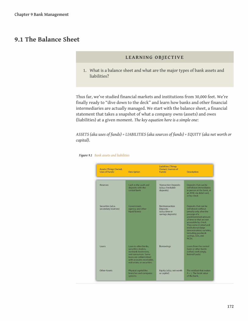
9.1 The Balance Sheet
LEARNING OBJECTIVE
1. What is a balance sheet and what are the major types of bank assets andliabilities?
Thus far, we’ve studied financial markets and institutions from 30,000 feet. We’refinally ready to “dive down to the deck” and learn how banks and other financialintermediaries are actually managed. We start with the balance sheet, a financialstatement that takes a snapshot of what a company owns (assets) and owes(liabilities) at a given moment. The key equation here is a simple one:
ASSETS (aka uses of funds) = LIABILITIES (aka sources of funds) + EQUITY (aka net worth orcapital).
Figure 9.1 Bank assets and liabilities
Chapter 9 Bank Management
172
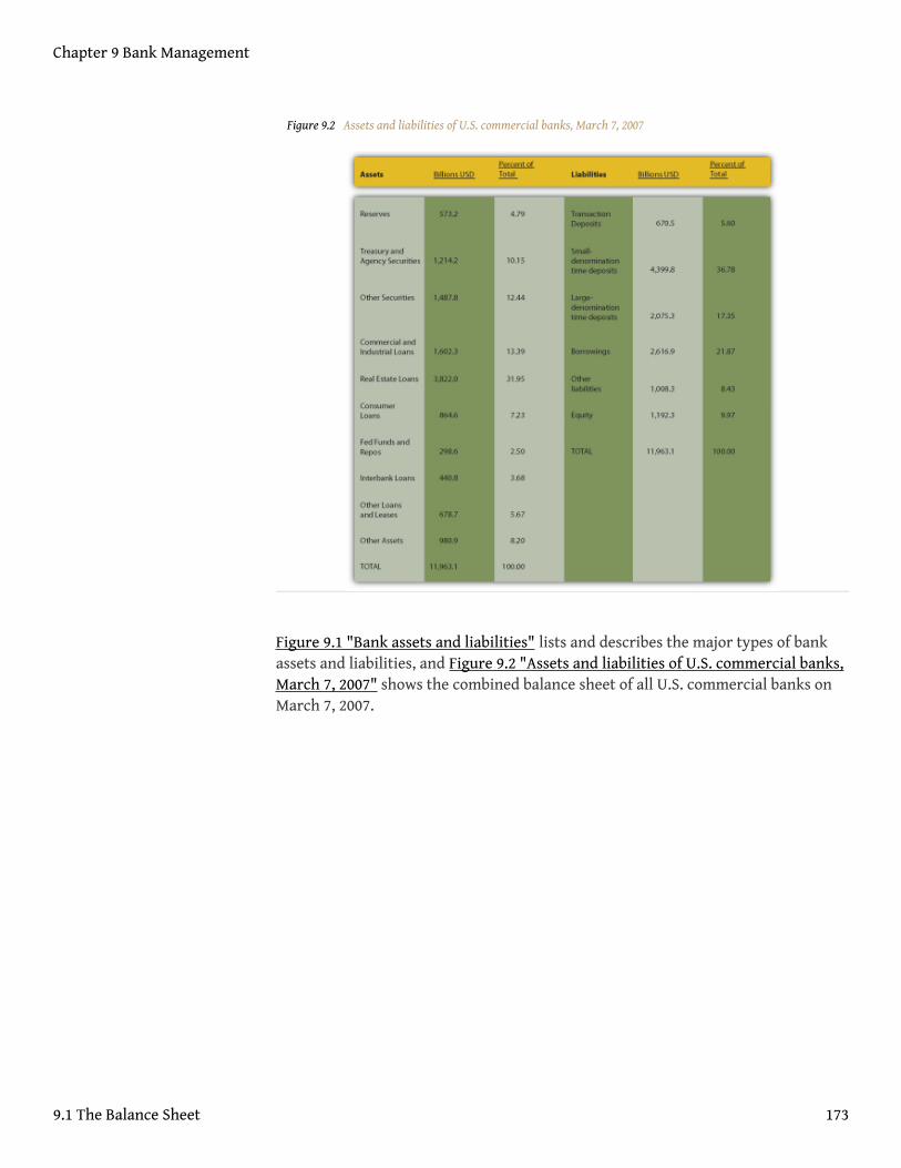
Figure 9.2 Assets and liabilities of U.S. commercial banks, March 7, 2007
Figure 9.1 "Bank assets and liabilities" lists and describes the major types of bankassets and liabilities, and Figure 9.2 "Assets and liabilities of U.S. commercial banks,March 7, 2007" shows the combined balance sheet of all U.S. commercial banks onMarch 7, 2007.
Chapter 9 Bank Management
9.1 The Balance Sheet 173
Stop and Think Box
In the first half of the nineteenth century, bank reserves1 in the United Statesconsisted solely of full-bodied specie (gold or silver) coins. Banks pledged to payspecie for both their notes and deposits immediately upon demand. Thegovernment did not mandate minimum reserve ratios. What level of reservesdo you think those banks kept? (Higher or lower than today’s requiredreserves2?) Why?
With some notorious exceptions known as wildcat banks, which were basicallyfinancial scams, banks kept reserves in the range of 20 to 30 percent, muchhigher than today’s required reserves. They did so for several reasons. First,unlike today, there was no fast, easy, cheap way for banks to borrow from thegovernment or other banks. They occasionally did so, but getting what wasneeded in time was far from assured. So basically borrowing was closed tothem. Banks in major cities like Boston, New York, and Philadelphia could keepsecondary reserves3, but before the advent of the telegraph, banks in thehinterland could not be certain that they could sell the volume of bonds theyneeded to into thin local markets. In those areas, which included most banks(by number), secondary reserves were of little use. And the potential for largenet outflows was higher than it is today because early bankers sometimescollected the liabilities of rival banks, then presented them all at once in thehopes of catching the other guy with inadequate specie reserves. Also, runs bydepositors were much more frequent then. There was only one thing for aprudent early banker to do: keep his or her vaults brimming with coins.
KEY TAKEAWAYS
• A balance sheet is a financial statement that lists what a company owns(its assets or uses of funds) and what it owes (its liabilities or sources offunds).
• Major bank assets include reserves, secondary reserves, loans, and otherassets.
• Major bank liabilities include deposits, borrowings, and shareholderequity.
1. In this context, cash funds thatbankers maintain to meetdeposit outflows and otherpayments.
2. A minimum amount of cashfunds that banks are requiredby regulators to hold.
3. Noncash, liquid assets, likegovernment bonds, thatbankers can quickly sell toobtain cash.
Chapter 9 Bank Management
9.1 The Balance Sheet 174
9.2 Assets, Liabilities, and T-Accounts
LEARNING OBJECTIVES
1. In five words, what do banks do?2. Without a word limitation, how would you describe what functions they
fulfill?
As Figure 9.1 "Bank assets and liabilities" and Figure 9.2 "Assets and liabilities ofU.S. commercial banks, March 7, 2007" show, commercial banks own reserves ofcash and deposits with the Fed; secondary reserves of government and other liquidsecurities; loans to businesses, consumers, and other banks; and other assets,including buildings, computer systems, and other physical stuff. Each of those assetsplays an important role in the bank’s overall business strategy. A bank’s physical assetsare needed to conduct its business, whether it be a traditional brick-and-mortarbank, a full e-commerce bank (there are servers and a headquarters someplace), ora hybrid click-and-mortar institution. Reserves allow banks to pay their transactiondeposits and other liabilities. In many countries, regulators mandate a minimumlevel of reserves, called required reserves. When banks hold more than the reserverequirement, the extra reserves are called excess reserves. Because reserves pay nointerest, American bankers generally keep excess reserves to a minimum,preferring instead to hold secondary reserves like U.S. Treasuries and other safe,liquid, interest-earning securities. Banks’ bread-and-butter asset is, of course, theirloans. They derive most of their income from loans, so they must be very carefulwho they lend to and on what terms. Banks lend to other banks via the federalfunds market, but also in the process of clearing checks, which are called “cashitems in process of collection.” Most of their loans, however, go to nonbanks. Someloans are uncollateralized, but many are backed by real estate (in which case theloans are called mortgages), accounts receivable (factorage), or securities (callloans).
Chapter 9 Bank Management
175
Stop and Think Box
Savings banks, a type of bank that issues only savings deposits, and lifeinsurance companies hold significantly fewer reserves than commercial banksdo. Why?
Savings banks and life insurance companies do not suffer large net outflowsvery often. People do draw down their savings by withdrawing money fromtheir savings accounts, cashing in their life insurance, or taking out policyloans, but remember that one of the advantages of relatively largeintermediaries is that they can often meet outflows from inflows. In otherwords, savings banks and life insurance companies can usually pay customerA’s withdrawal (policy loan or surrender) from customer B’s deposit (premiumpayment). Therefore, they have no need to carry large reserves, which areexpensive in terms of opportunity costs.
Where do banks get the wherewithal to purchase those assets? The right-hand side ofthe balance sheet lists a bank’s liabilities or the sources of its funds. Transaction depositsinclude negotiable order of withdrawal accounts (NOW) and money market depositaccounts (MMDAs), in addition to good old checkable deposits. Banks liketransaction deposits because they can avoid paying much, if any, interest on them.Some depositors find the liquidity that transaction accounts provide so convenientthey even pay for the privilege of keeping their money in the bank via various fees,of which more anon. Banks justify the fees by pointing out that it is costly to keepthe books, transfer money, and maintain sufficient cash reserves to meetwithdrawals.
The administrative costs of nontransaction deposits are lower so banks pay interestfor those funds. Nontransaction deposits range from the traditional passbooksavings account to negotiable certificates of deposit (NCDs) with denominationsgreater than $100,000. Checks cannot be drawn on passbook savings accounts, butdepositors can withdraw from or add to the account at will. Because they are moreliquid, they pay lower rates of interest than time deposits (aka certificates ofdeposit), which impose stiff penalties for early withdrawals. Banks also borrowoutright from other banks overnight via what is called, strangely, the federal fundsmarket, and directly from the Federal Reserve via discount loans (aka advances).They can also borrow from corporations, including their parent companies if theyare part of a bank holding company4.4. A corporate entity than owns
one or more banks andbanking-related subsidiaries.
Chapter 9 Bank Management
9.2 Assets, Liabilities, and T-Accounts 176
That leaves only bank net worth, the difference between the value of a bank’s assets and itsliabilities. Equity originally comes from stockholders when they pay for shares in thebank’s initial public offering (IPO) or direct public offering (DPO). Later, it comesmostly from retained earnings, but sometimes banks make a seasoned offering ofadditional stock. Regulators watch bank capital closely because, as we learned inChapter 8 "Financial Structure, Transaction Costs, and Asymmetric Information",the more equity a bank has, the less likely it is that it will fail. Today, havinglearned this lesson the hard way, U.S. regulators will close a bank down well beforeits equity reaches zero. Provided, that is, they catch it first. Even well-capitalizedbanks can fail very quickly, especially if they trade in the derivatives market, ofwhich more below.
At the broadest level, banks and other financial intermediaries engage in assettransformation. In other words, they sell liabilities with certain liquidity, risk, return,and denominational characteristics and use those funds to buy assets with a different set ofcharacteristics. Intermediaries link investors (purchasers of banks’ liabilities) toentrepreneurs (sellers of banks’ assets) in a more sophisticated way than meremarket facilitators like dealer-brokers and peer-to-peer bankers do (see Chapter 8"Financial Structure, Transaction Costs, and Asymmetric Information").
More specifically, banks (aka depository institutions) turn short-term deposits intolong-term loans. In other words, they borrow short and lend long. This, we’ll see,makes bank management tricky business indeed. Other financial intermediariestransform assets in other ways. Finance companies borrow long and lend short,rendering their management much easier than that of a bank. Life insurancecompanies sell contracts (called policies) that pay off when or if (during the policyperiod of a term policy) the insured party dies. Property and casualty companiessell policies that pay if some exigency, like an automobile crash, occurs during thepolicy period. The liabilities of insurance companies are said to be contingentbecause they come due if an event happens rather than after a specified period oftime.
Asset transformation and balance sheets provide us with only a snapshot view of afinancial intermediary’s business. That’s useful, but, of course, intermediaries, likebanks, are dynamic places where changes constantly occur. The easiest way to analyzethat dynamism is via so-called T-accounts, simplified balance sheets that list only changes inliabilities and assets. By the way, they are called T-accounts because they look like aT. Sort of. Note in the T-accounts below the horizontal and vertical rules that crosseach other, sort of like a T.
Suppose somebody deposits $17.52 in cash in a checking account. The T-account forthe bank accepting the deposit would be the following:
Chapter 9 Bank Management
9.2 Assets, Liabilities, and T-Accounts 177
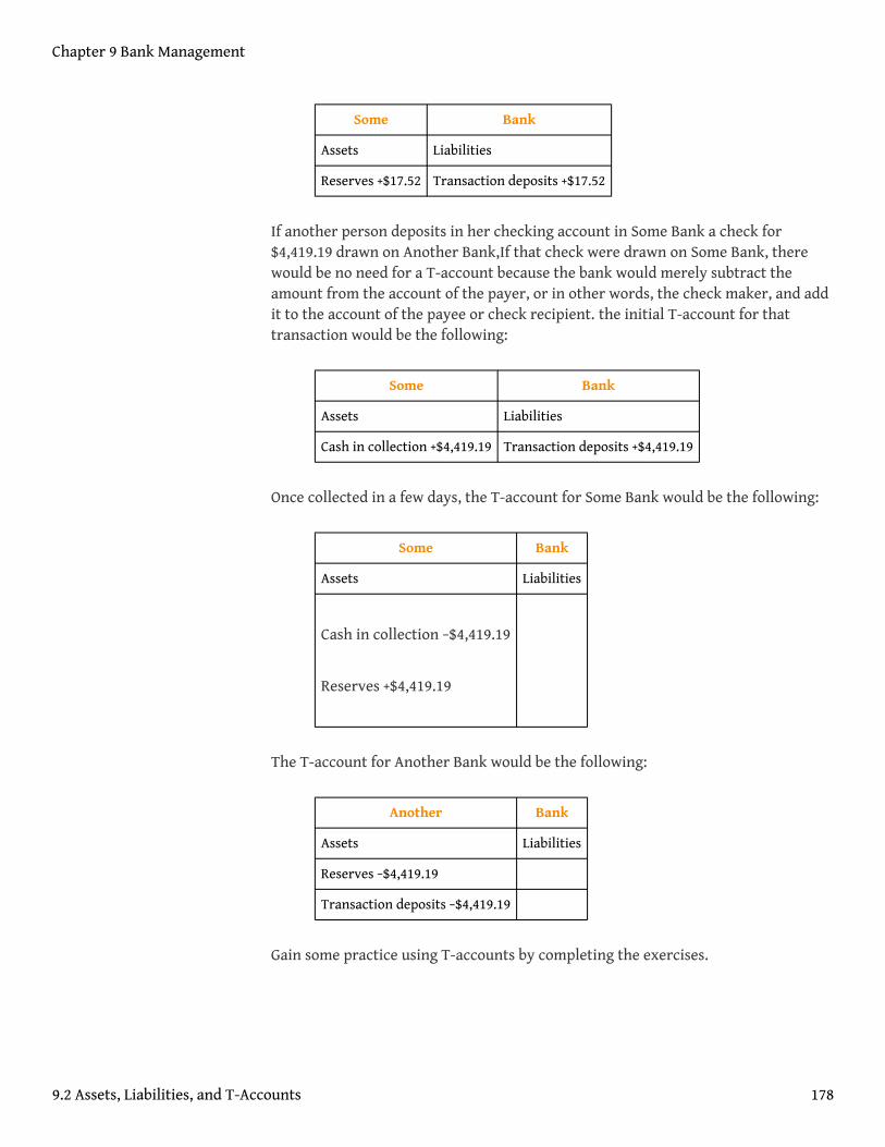
Some Bank
Assets Liabilities
Reserves +$17.52 Transaction deposits +$17.52
If another person deposits in her checking account in Some Bank a check for$4,419.19 drawn on Another Bank,If that check were drawn on Some Bank, therewould be no need for a T-account because the bank would merely subtract theamount from the account of the payer, or in other words, the check maker, and addit to the account of the payee or check recipient. the initial T-account for thattransaction would be the following:
Some Bank
Assets Liabilities
Cash in collection +$4,419.19 Transaction deposits +$4,419.19
Once collected in a few days, the T-account for Some Bank would be the following:
Some Bank
Assets Liabilities
Cash in collection −$4,419.19
Reserves +$4,419.19
The T-account for Another Bank would be the following:
Another Bank
Assets Liabilities
Reserves −$4,419.19
Transaction deposits −$4,419.19
Gain some practice using T-accounts by completing the exercises.
Chapter 9 Bank Management
9.2 Assets, Liabilities, and T-Accounts 178
EXERCISES
Write out the T-accounts for the following transactions.
1. Larry closes his $73,500.88 account with JPMC Bank, spends $500.88 ofthat money on consumption goods, then places the rest in W Bank.
2. Suppose regulators tell W Bank that it needs to hold only 5 percent ofthose transaction deposits in reserve.
3. W Bank decides that it needs to hold no excess reserves but needs tobolster its secondary reserves.
4. A depositor in W bank decides to move $7,000 from her checkingaccount to a CD in W Bank.
5. W Bank sells $500,000 of Treasuries and uses the proceeds tofund two $200,000 mortgages and the purchase of $100,000 ofmunicipal bonds.
(Note: This is net. The bank merely moved $100,000 from one typeof security to another.)
KEY TAKEAWAYS
• In five words, banks lend (1) long (2) and (3) borrow (4) short (5).• Like other financial intermediaries, banks are in the business of
transforming assets, of issuing liabilities with one set of characteristicsto investors and of buying the liabilities of borrowers with another set ofcharacteristics.
• Generally, banks issue short-term liabilities but buy long-term assets.• This raises specific types of management problems that bankers must be
proficient at solving if they are to succeed.
Chapter 9 Bank Management
9.2 Assets, Liabilities, and T-Accounts 179
9.3 Bank Management Principles
LEARNING OBJECTIVE
1. What are the major problems facing bank managers and why is bankmanagement closely regulated?
Bankers must manage their assets and liabilities to ensure three conditions:
1. Their bank has enough reserves on hand to pay for any deposit outflows (netdecreases in deposits) but not so many as to render the bank unprofitable.This tricky trade-off is called liquidity management5.
2. Their bank earns profits. To do so, the bank must own a diverse portfolioof remunerative assets. This is known as asset management6. It mustalso obtain its funds as cheaply as possible, which is known as liabilitymanagement7.
3. Their bank has sufficient net worth or equity capital to maintain a cushionagainst bankruptcy or regulatory attention but not so much that the bank isunprofitable. This second tricky trade-off is called capital adequacymanagement8.
In their quest to earn profits and manage liquidity and capital, banks face twomajor risks: credit risk, the risk of borrowers defaulting on the loans and securitiesit owns, and interest rate risk, the risk that interest rate changes will decrease thereturns on its assets and/or increase the cost of its liabilities. The financial panic of2008 reminded bankers that they also can face liability and capital adequacy risks iffinancial markets become less liquid or seize up completely (q* = 0).
5. Ensuring that the bank has justthe right amount ofreserves—not too little, whichwould endanger the bank’ssolvency, nor too much, whichwould decrease itsprofitability.
6. Ensuring that the bank’s assetshave the right combination ofliquidity, safety, and return.
7. Attracting enough deposits orborrowing enough to ensurethat the bank can make theloans or purchase the assets itwants.
8. Ensuring that the bank hasenough capital, equity, or networth to remain in operationwhile maintaining bankprofitability as measured byreturn on equity (ROE).
Chapter 9 Bank Management
180
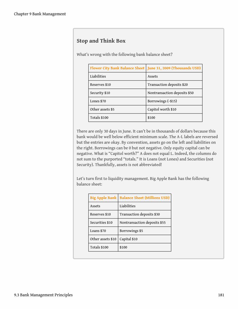
Stop and Think Box
What’s wrong with the following bank balance sheet?
Flower City Bank Balance Sheet June 31, 2009 (Thousands USD)
Liabilities Assets
Reserves $10 Transaction deposits $20
Security $10 Nontransaction deposits $50
Lones $70 Borrowings (−$15)
Other assets $5 Capitol worth $10
Totals $100 $100
There are only 30 days in June. It can’t be in thousands of dollars because thisbank would be well below efficient minimum scale. The A-L labels are reversedbut the entries are okay. By convention, assets go on the left and liabilities onthe right. Borrowings can be 0 but not negative. Only equity capital can benegative. What is “Capitol worth?” A does not equal L. Indeed, the columns donot sum to the purported “totals.” It is Loans (not Lones) and Securities (notSecurity). Thankfully, assets is not abbreviated!
Let’s turn first to liquidity management. Big Apple Bank has the followingbalance sheet:
Big Apple Bank Balance Sheet (Millions USD)
Assets Liabilities
Reserves $10 Transaction deposits $30
Securities $10 Nontransaction deposits $55
Loans $70 Borrowings $5
Other assets $10 Capital $10
Totals $100 $100
Chapter 9 Bank Management
9.3 Bank Management Principles 181
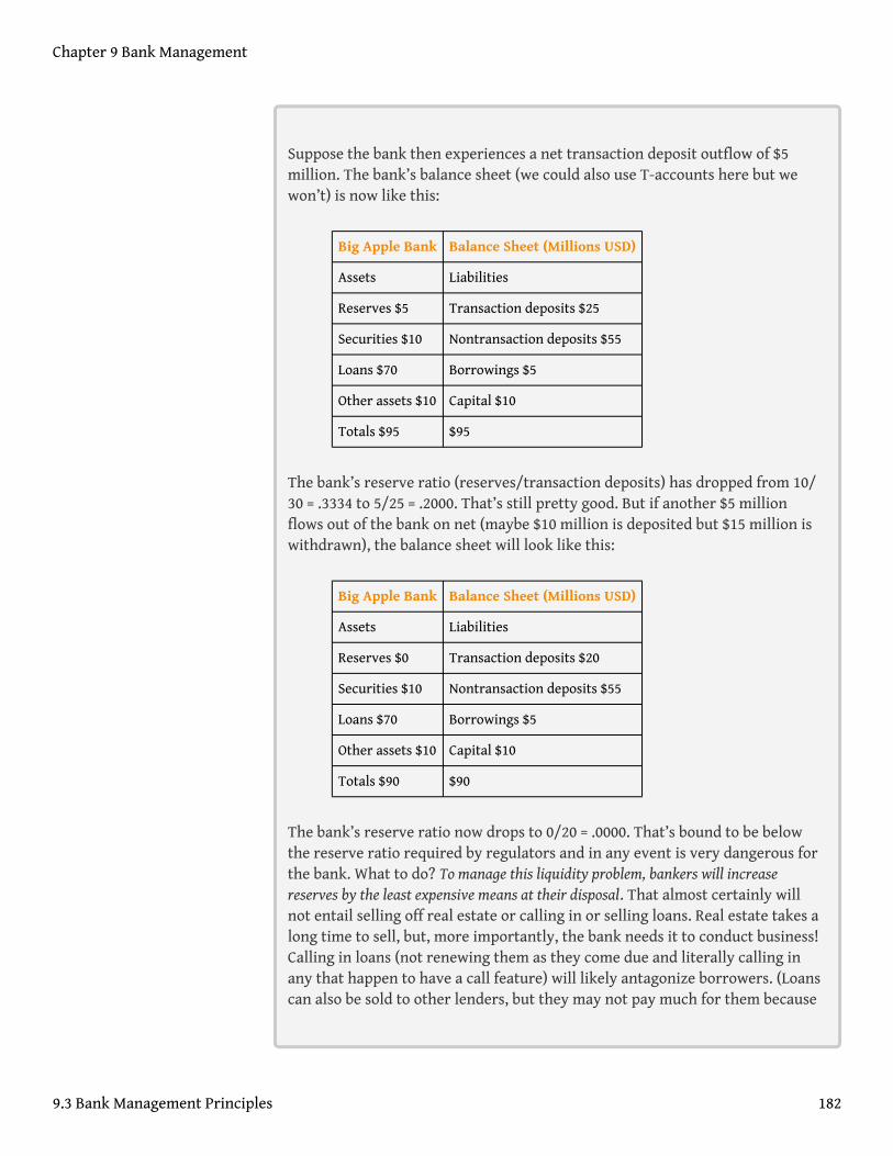
Suppose the bank then experiences a net transaction deposit outflow of $5million. The bank’s balance sheet (we could also use T-accounts here but wewon’t) is now like this:
Big Apple Bank Balance Sheet (Millions USD)
Assets Liabilities
Reserves $5 Transaction deposits $25
Securities $10 Nontransaction deposits $55
Loans $70 Borrowings $5
Other assets $10 Capital $10
Totals $95 $95
The bank’s reserve ratio (reserves/transaction deposits) has dropped from 10/30 = .3334 to 5/25 = .2000. That’s still pretty good. But if another $5 millionflows out of the bank on net (maybe $10 million is deposited but $15 million iswithdrawn), the balance sheet will look like this:
Big Apple Bank Balance Sheet (Millions USD)
Assets Liabilities
Reserves $0 Transaction deposits $20
Securities $10 Nontransaction deposits $55
Loans $70 Borrowings $5
Other assets $10 Capital $10
Totals $90 $90
The bank’s reserve ratio now drops to 0/20 = .0000. That’s bound to be belowthe reserve ratio required by regulators and in any event is very dangerous forthe bank. What to do? To manage this liquidity problem, bankers will increasereserves by the least expensive means at their disposal. That almost certainly willnot entail selling off real estate or calling in or selling loans. Real estate takes along time to sell, but, more importantly, the bank needs it to conduct business!Calling in loans (not renewing them as they come due and literally calling inany that happen to have a call feature) will likely antagonize borrowers. (Loanscan also be sold to other lenders, but they may not pay much for them because
Chapter 9 Bank Management
9.3 Bank Management Principles 182
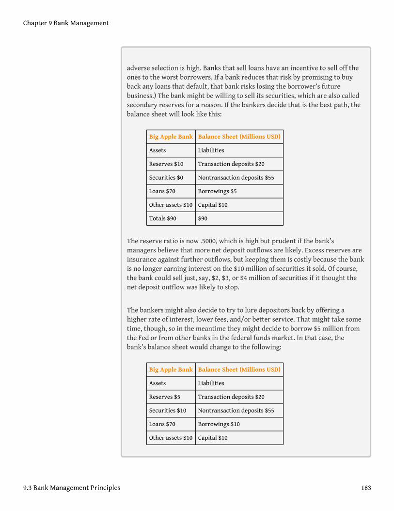
adverse selection is high. Banks that sell loans have an incentive to sell off theones to the worst borrowers. If a bank reduces that risk by promising to buyback any loans that default, that bank risks losing the borrower’s futurebusiness.) The bank might be willing to sell its securities, which are also calledsecondary reserves for a reason. If the bankers decide that is the best path, thebalance sheet will look like this:
Big Apple Bank Balance Sheet (Millions USD)
Assets Liabilities
Reserves $10 Transaction deposits $20
Securities $0 Nontransaction deposits $55
Loans $70 Borrowings $5
Other assets $10 Capital $10
Totals $90 $90
The reserve ratio is now .5000, which is high but prudent if the bank’smanagers believe that more net deposit outflows are likely. Excess reserves areinsurance against further outflows, but keeping them is costly because the bankis no longer earning interest on the $10 million of securities it sold. Of course,the bank could sell just, say, $2, $3, or $4 million of securities if it thought thenet deposit outflow was likely to stop.
The bankers might also decide to try to lure depositors back by offering ahigher rate of interest, lower fees, and/or better service. That might take sometime, though, so in the meantime they might decide to borrow $5 million fromthe Fed or from other banks in the federal funds market. In that case, thebank’s balance sheet would change to the following:
Big Apple Bank Balance Sheet (Millions USD)
Assets Liabilities
Reserves $5 Transaction deposits $20
Securities $10 Nontransaction deposits $55
Loans $70 Borrowings $10
Other assets $10 Capital $10
Chapter 9 Bank Management
9.3 Bank Management Principles 183
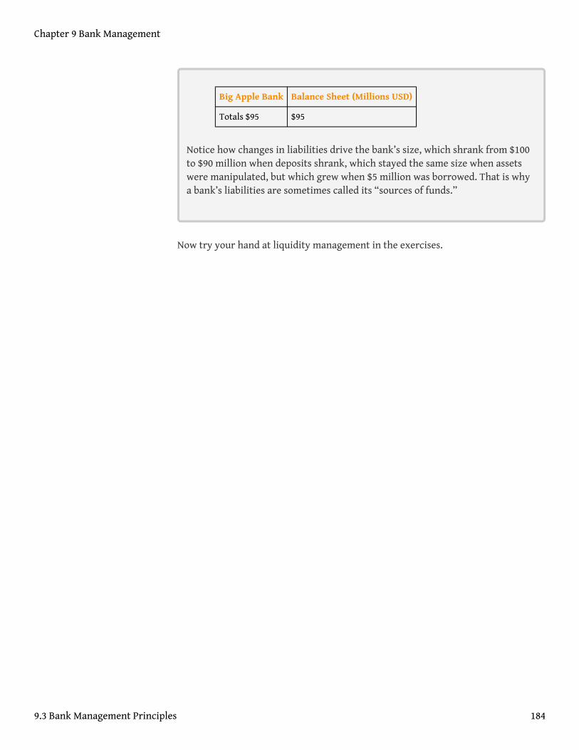
Big Apple Bank Balance Sheet (Millions USD)
Totals $95 $95
Notice how changes in liabilities drive the bank’s size, which shrank from $100to $90 million when deposits shrank, which stayed the same size when assetswere manipulated, but which grew when $5 million was borrowed. That is whya bank’s liabilities are sometimes called its “sources of funds.”
Now try your hand at liquidity management in the exercises.
Chapter 9 Bank Management
9.3 Bank Management Principles 184
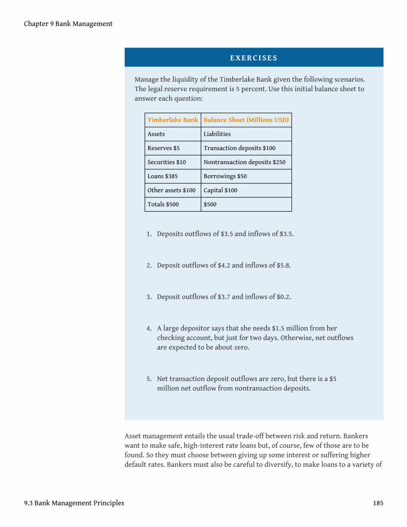
EXERCISES
Manage the liquidity of the Timberlake Bank given the following scenarios.The legal reserve requirement is 5 percent. Use this initial balance sheet toanswer each question:
Timberlake Bank Balance Sheet (Millions USD)
Assets Liabilities
Reserves $5 Transaction deposits $100
Securities $10 Nontransaction deposits $250
Loans $385 Borrowings $50
Other assets $100 Capital $100
Totals $500 $500
1. Deposits outflows of $3.5 and inflows of $3.5.
2. Deposit outflows of $4.2 and inflows of $5.8.
3. Deposit outflows of $3.7 and inflows of $0.2.
4. A large depositor says that she needs $1.5 million from herchecking account, but just for two days. Otherwise, net outflowsare expected to be about zero.
5. Net transaction deposit outflows are zero, but there is a $5million net outflow from nontransaction deposits.
Asset management entails the usual trade-off between risk and return. Bankerswant to make safe, high-interest rate loans but, of course, few of those are to befound. So they must choose between giving up some interest or suffering higherdefault rates. Bankers must also be careful to diversify, to make loans to a variety of
Chapter 9 Bank Management
9.3 Bank Management Principles 185
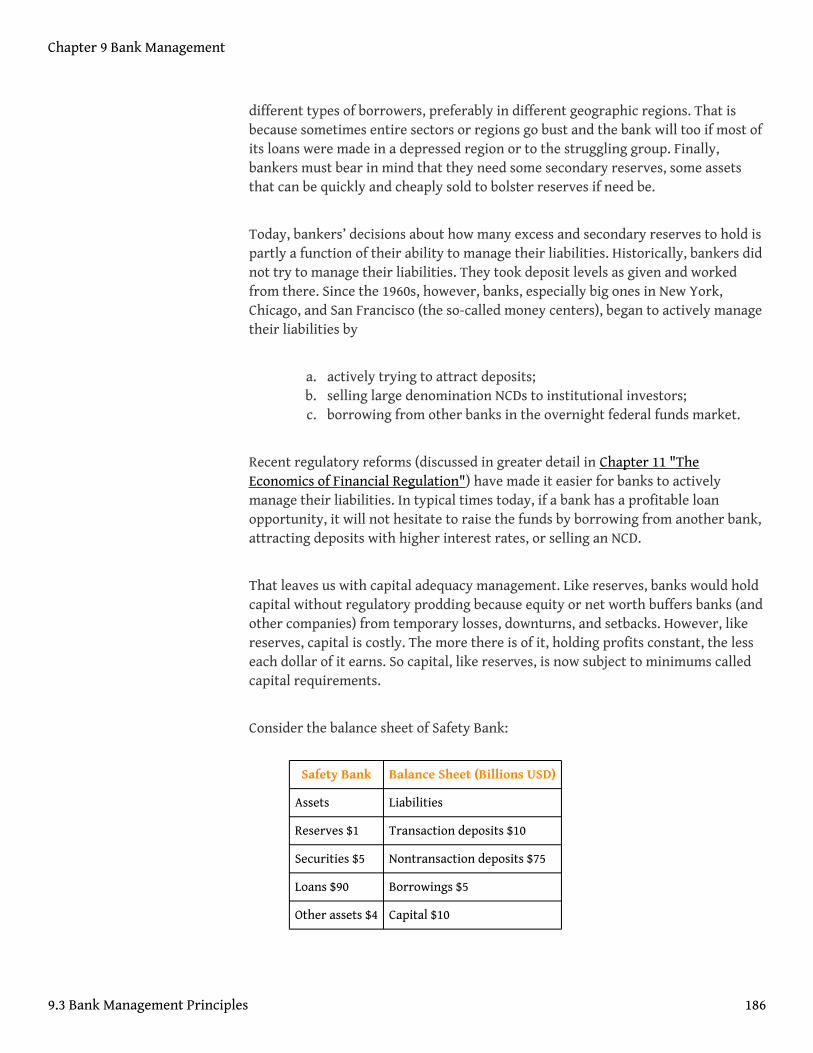
different types of borrowers, preferably in different geographic regions. That isbecause sometimes entire sectors or regions go bust and the bank will too if most ofits loans were made in a depressed region or to the struggling group. Finally,bankers must bear in mind that they need some secondary reserves, some assetsthat can be quickly and cheaply sold to bolster reserves if need be.
Today, bankers’ decisions about how many excess and secondary reserves to hold ispartly a function of their ability to manage their liabilities. Historically, bankers didnot try to manage their liabilities. They took deposit levels as given and workedfrom there. Since the 1960s, however, banks, especially big ones in New York,Chicago, and San Francisco (the so-called money centers), began to actively managetheir liabilities by
a. actively trying to attract deposits;b. selling large denomination NCDs to institutional investors;c. borrowing from other banks in the overnight federal funds market.
Recent regulatory reforms (discussed in greater detail in Chapter 11 "TheEconomics of Financial Regulation") have made it easier for banks to activelymanage their liabilities. In typical times today, if a bank has a profitable loanopportunity, it will not hesitate to raise the funds by borrowing from another bank,attracting deposits with higher interest rates, or selling an NCD.
That leaves us with capital adequacy management. Like reserves, banks would holdcapital without regulatory prodding because equity or net worth buffers banks (andother companies) from temporary losses, downturns, and setbacks. However, likereserves, capital is costly. The more there is of it, holding profits constant, the lesseach dollar of it earns. So capital, like reserves, is now subject to minimums calledcapital requirements.
Consider the balance sheet of Safety Bank:
Safety Bank Balance Sheet (Billions USD)
Assets Liabilities
Reserves $1 Transaction deposits $10
Securities $5 Nontransaction deposits $75
Loans $90 Borrowings $5
Other assets $4 Capital $10
Chapter 9 Bank Management
9.3 Bank Management Principles 186
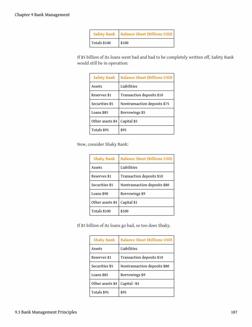
Safety Bank Balance Sheet (Billions USD)
Totals $100 $100
If $5 billion of its loans went bad and had to be completely written off, Safety Bankwould still be in operation:
Safety Bank Balance Sheet (Billions USD)
Assets Liabilities
Reserves $1 Transaction deposits $10
Securities $5 Nontransaction deposits $75
Loans $85 Borrowings $5
Other assets $4 Capital $5
Totals $95 $95
Now, consider Shaky Bank:
Shaky Bank Balance Sheet (Billions USD)
Assets Liabilities
Reserves $1 Transaction deposits $10
Securities $5 Nontransaction deposits $80
Loans $90 Borrowings $9
Other assets $4 Capital $1
Totals $100 $100
If $5 billion of its loans go bad, so too does Shaky.
Shaky Bank Balance Sheet (Billions USD)
Assets Liabilities
Reserves $1 Transaction deposits $10
Securities $5 Nontransaction deposits $80
Loans $85 Borrowings $9
Other assets $4 Capital −$4
Totals $95 $95
Chapter 9 Bank Management
9.3 Bank Management Principles 187
You don’t need to be a certified public accountant (CPA) to know that red numbersand negative signs are not good news. Shaky Bank is a now a new kind of bank,bankrupt.
Why would a banker manage capital like Shaky Bank instead of like Safety Bank? Ina word, profitability. There are two major ways of measuring profitability: returnon assets (ROA) and return on equity (ROE).
ROA = net after-tax profit/assets
ROE = net after-tax profit/equity (capital, net worth)
Suppose that, before the loan debacle, both Safety and Shaky Bank had $10 billionin profits. The ROA of both would be 10/100 = .10. But Shaky Bank’s ROE, whatshareholders care about most, would leave Safety Bank in the dust because Shaky Bank ismore highly leveraged (more assets per dollar of equity).
Shaky Bank ROE = 10/1 = 10
Safety Bank ROE = 10/10 = 1
This, of course, is nothing more than the standard risk-return trade-off applied tobanking. Regulators in many countries have therefore found it prudent to mandate capitaladequacy standards to ensure that some bankers are not taking on high levels of risk in thepursuit of high profits.
Bankers manage bank capital in several ways:
a. By buying (selling) their own bank’s stock in the open market. Thatreduces (increases) the number of shares outstanding, raising(decreasing) capital and ROE, ceteris paribus
b. By paying (withholding) dividends, which decreases (increases) capital,increasing (decreasing) ROE, all else equal
c. By increasing (decreasing) the bank’s assets, which, with capital heldconstant, increases (decreases) ROE
These same concepts and principles—asset, liability, capital, and liquiditymanagement, and capital-liquidity and capital-profitability trade-offs—apply toother types of financial intermediaries as well, though the details, of course, differ.
Chapter 9 Bank Management
9.3 Bank Management Principles 188
KEY TAKEAWAYS
• Bankers must manage their bank’s liquidity (reserves, for regulatoryreasons and to conduct business effectively), capital (for regulatoryreasons and to buffer against negative shocks), assets, and liabilities.
• There is an opportunity cost to holding reserves, which pay no interest,and capital, which must share the profits of the business.
• Left to their own judgment, bankers would hold reserves > 0 and capital> 0, but they might not hold enough to prevent bank failures at what thegovernment or a country’s citizens deem an acceptably low rate.
• That induces government regulators to create and monitor minimumrequirements.
Chapter 9 Bank Management
9.3 Bank Management Principles 189
9.4 Credit Risk
LEARNING OBJECTIVE
1. What is credit risk and how do bankers manage it?
As noted above, loans are banks’ bread and butter. No matter how good bankers are atasset, liability, and capital adequacy management, they will be failures if they cannotmanage credit risk. Keeping defaults to a minimum requires bankers to be keenstudents of asymmetric information (adverse selection and moral hazard) andtechniques for reducing them.
Bankers and insurers, like computer folks, know about GIGO—garbage in, garbageout. If they lend to or insure risky people and companies, they are going to suffer.So they carefully screen applicants for loans and insurance. In other words, toreduce asymmetric information, financial intermediaries create information about them.One way they do so is to ask applicants a wide variety of questions.
Financial intermediaries use the application only as a starting point. Because riskyapplicants might stretch the truth or even outright lie on the application, intermediariestypically do two things: (1) make the application a binding part of the financial contract, and(2) verify the information with disinterested third parties. The first allows them to voidcontracts if applications are fraudulent. If someone applied for life insurance butdid not disclose that he or she was suffering from a terminal disease, the lifeinsurance company would not pay, though it might return any premiums. (Thatmay sound cruel to you, but it isn’t. In the process of protecting its profits, theinsurance company is also protecting its policyholders.) In other situations, theintermediary might not catch a falsehood in an application until it is too late, so italso verifies important information by calling employers (Is John Doe really theSupreme Commander of XYZ Corporation?), conducting medical examinations (IsJane Smith really in perfect health despite being 3' 6'' tall and weighing 567pounds?), hiring appraisers (Is a one-bedroom, half-bath house on the wrong side ofthe tracks really worth $1.2 million?), and so forth. Financial intermediaries canalso buy credit reports from third-party report providers like Equifax, Experian, orTrans Union. Similarly, insurance companies regularly share information with eachother so that risky applicants can’t take advantage of them easily.
To help improve their screening acumen, many financial intermediaries specialize. Bymaking loans to only one or a few types of borrowers, by insuring automobiles in a
Chapter 9 Bank Management
190
handful of states, by insuring farms but not factories, intermediaries get very goodat discerning risky applicants from the rest. Specialization also helps to keepmonitoring costs to a minimum. Remember that, to reduce moral hazard(postcontractual asymmetric information), intermediaries have to pay attention towhat borrowers and people who are insured do. By specializing, intermediariesknow what sort of restrictive covenants (aka loan covenants) to build into theircontracts. Loan covenants include the frequency of providing financial reports, thetypes of information to be provided in said reports, working capital requirements,permission for onsite inspections, limitations on account withdrawals, and calloptions if business performance deteriorates as measured by specific businessratios. Insurance companies also build covenants into their contracts. You can’tturn your home into a brothel, it turns out, and retain your insurance coverage. Toreduce moral hazard further, insurers also investigate claims that seem fishy. If youwrap your car around a tree the day after insuring it or increasing your coverage,the insurer’s claims adjuster is probably going to take a very close look at thealleged accident. Like everything else in life, however, specialization has its costs.Some companies overspecialize, hurting their asset management by making toomany loans or issuing too many policies in one place or to one group. While creditrisks decrease due to specialization, systemic risk to assets increases, requiring bankers tomake difficult decisions regarding how much to specialize.
Forging long-term relationships with customers can also help financial intermediaries tomanage their credit risks. Bankers, for instance, can lend with better assurance if theycan study the checking and savings accounts of applicants over a period of years ordecades. Repayment records of applicants who had previously obtained loans canbe checked easily and cheaply. Moreover, the expectation (there’s that word again)of a long-term relationship changes the borrower’s calculations. The game, if youwill, is no longer a one-off prisoner’s dilemma,http://plato.stanford.edu/entries/prisoner-dilemma/ where it is in both parties’ interest to defect, but rather arepeated game, where the optimal strategy is one of tit for tat—cooperate until theother guy defects.http://www.gametheory.net/dictionary/TitforTat.html
One way that lenders create long-term relationships with businesses is by providing loancommitments, promises to lend $x at y interest (or y plus some market rate) for z years.Such arrangements are so beneficial for both lenders and borrowers that mostcommercial loans are in fact loan commitments. Such commitments are sometimescalled lines of credit, particularly when extended to consumers.
Bankers also often insist on collateral—assets pledged by the borrower for repaymentof a loan. When those assets are cash left in the bank, the collateral is calledcompensating or compensatory balances. Another powerful tool to combat asymmetricinformation is credit rationing, refusing to make a loan at any interest rate (to reduceadverse selection) or lending less than the sum requested (to reduce moral hazard). Insurers
Chapter 9 Bank Management
9.4 Credit Risk 191
also engage in both types of rationing, and for the same reasons: people willing topay high rates or premiums must be risky, and the more that is lent or insured(ceteris paribus) the higher the likelihood that the customer will abscond, cheat, orset aflame, as the case may be.
As the world learned to its chagrin in 2007–2008, banks and other lenders are notperfect screeners. Sometimes, under competitive pressure, they lend to borrowersthey should not have. Sometimes, individual bankers profit handsomely by lendingto very risky borrowers, even though their actions endanger their banks’ veryexistence. Other times, external political or societal pressures induce bankers tomake loans they normally wouldn’t. Such excesses are always reversed eventuallybecause the lenders suffer from high levels of nonperforming loans9.
Stop and Think Box
In the first quarter of 2007, banks and other intermediaries specializing inoriginating home mortgages (called mortgage companies) experienced a majorsetback in the so-called subprime market, the segment of the market thatcaters to high-risk borrowers, because default rates soared much higher thanexpected. Losses were so extensive that many people feared, correctly as itturned out, that they could trigger a financial crisis. To stave off such apotentially dangerous outcome, why didn’t the government immediatelyintervene by guaranteeing the subprime mortgages?
The government must be careful to try to support the financial system withoutgiving succor to those who have screwed up. Directly bailing out the subprimelenders by guaranteeing mortgage payments would cause moral hazard toskyrocket, it realized. Borrowers might be more likely to default byrationalizing that the crime is a victimless one (though, in fact, all taxpayerswould suffer—recall that there is no such thing as a free lunch in economics).Lenders would learn that they can make crazy loans to anyone because good ol’Uncle Sam will cushion, or even prevent, their fall.
9. A loan that is in default, wherethe borrower is not makingstipulated payments of interestor principal.
Chapter 9 Bank Management
9.4 Credit Risk 192
KEY TAKEAWAYS
• Credit risk is the chance that a borrower will default on a loan by notfully meeting stipulated payments on time.
• Bankers manage credit risk by screening applicants (taking applicationsand verifying the information they contain), monitoring loan recipients,requiring collateral like real estate and compensatory balances, andincluding a variety of restrictive covenants in loans.
• They also manage credit risk by trading off between the costs andbenefits of specialization and portfolio diversification.
Chapter 9 Bank Management
9.4 Credit Risk 193
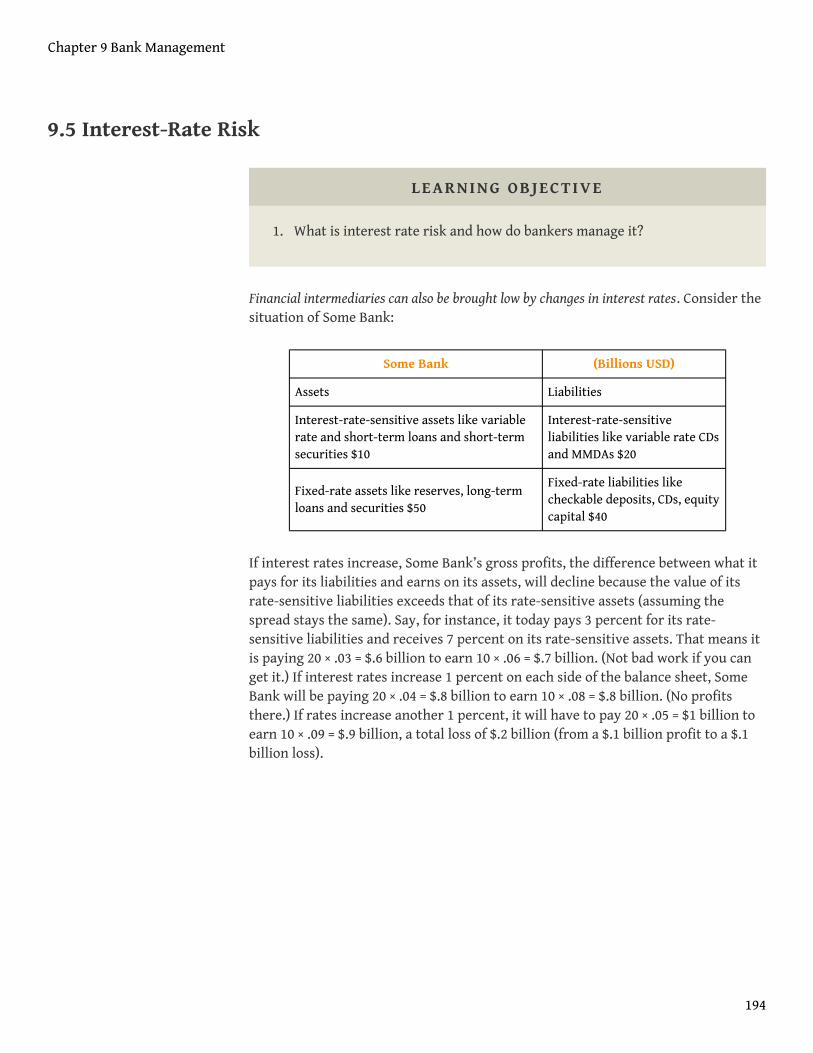
9.5 Interest-Rate Risk
LEARNING OBJECTIVE
1. What is interest rate risk and how do bankers manage it?
Financial intermediaries can also be brought low by changes in interest rates. Consider thesituation of Some Bank:
Some Bank (Billions USD)
Assets Liabilities
Interest-rate-sensitive assets like variablerate and short-term loans and short-termsecurities $10
Interest-rate-sensitiveliabilities like variable rate CDsand MMDAs $20
Fixed-rate assets like reserves, long-termloans and securities $50
Fixed-rate liabilities likecheckable deposits, CDs, equitycapital $40
If interest rates increase, Some Bank’s gross profits, the difference between what itpays for its liabilities and earns on its assets, will decline because the value of itsrate-sensitive liabilities exceeds that of its rate-sensitive assets (assuming thespread stays the same). Say, for instance, it today pays 3 percent for its rate-sensitive liabilities and receives 7 percent on its rate-sensitive assets. That means itis paying 20 × .03 = $.6 billion to earn 10 × .06 = $.7 billion. (Not bad work if you canget it.) If interest rates increase 1 percent on each side of the balance sheet, SomeBank will be paying 20 × .04 = $.8 billion to earn 10 × .08 = $.8 billion. (No profitsthere.) If rates increase another 1 percent, it will have to pay 20 × .05 = $1 billion toearn 10 × .09 = $.9 billion, a total loss of $.2 billion (from a $.1 billion profit to a $.1billion loss).
Chapter 9 Bank Management
194
Stop and Think Box
Inflation was unexpectedly high in the 1970s. Given what you learned about therelationship between inflation and nominal interest rates in Chapter 5 "TheEconomics of Interest-Rate Fluctuations", and between interest rates and bankprofitability in this chapter, what happened in the 1980s?
Bank profitability sank to the point that many banks, the infamous savings andloans (S&Ls), went under. Inflation (via the Fisher Equation) caused nominalinterest rates to increase, which hurt banks’ profitability because they wereearning low rates on long-term assets (like thirty-year bonds) while having topay high rates on their short-term liabilities. Mounting losses induced manybankers to take on added risks, including risks in the derivatives markets. A fewrestored their banks to profitability, but others destroyed all of their bank’scapital and then some.
Of course, if the value of its risk-sensitive assets exceeded that of its liabilities, the bankwould profit from interest rate increases. It would suffer, though, if interest ratesdecreased. Imagine Some Bank has $10 billion in interest rate-sensitive assets at 8percent and only $1 billion in interest rate-sensitive liabilities at 5 percent. It isearning 10 × .08 = $.8 billion while paying 1 × .05 = $.05 billion. If interest ratesdecreased, it might earn only 10 × .05 = $.5 billion while paying 1 × .02 = $.02 billion;thus, ceteris paribus, its gross profits would decline from .8 − .05 = $.75 billion to .5 −.02 = $.48 billion, a loss of $.27 billion. More formally, this type of calculation, calledbasic gap analysis, is
where:
Cρ = changes in profitability
Ar = risk-sensitive assets
Lr = risk-sensitive liabilities
Δi = change in interest rates
Cρ = (A r − Lr) × △ i
Chapter 9 Bank Management
9.5 Interest-Rate Risk 195
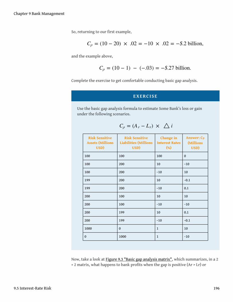
So, returning to our first example,
and the example above,
Complete the exercise to get comfortable conducting basic gap analysis.
EXERCISE
Use the basic gap analysis formula to estimate Some Bank’s loss or gainunder the following scenarios.
Risk SensitiveAssets (Millions
USD)
Risk SensitiveLiabilities (Millions
USD)
Change inInterest Rates
(%)
Answer: CP
(MillionsUSD)
100 100 100 0
100 200 10 −10
100 200 −10 10
199 200 10 −0.1
199 200 −10 0.1
200 100 10 10
200 100 −10 −10
200 199 10 0.1
200 199 −10 −0.1
1000 0 1 10
0 1000 1 −10
Now, take a look at Figure 9.3 "Basic gap analysis matrix", which summarizes, in a 2× 2 matrix, what happens to bank profits when the gap is positive (Ar > Lr) or
Cρ = (10 − 20) × .02 = −10 × .02 = −$.2 billion,
Cρ = (10 − 1) − (−.03) = −$.27 billion.
Cρ = (A r − Lr) × △ i
Chapter 9 Bank Management
9.5 Interest-Rate Risk 196
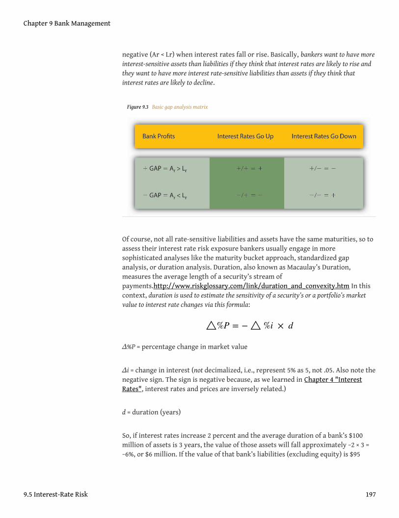
negative (Ar < Lr) when interest rates fall or rise. Basically, bankers want to have moreinterest-sensitive assets than liabilities if they think that interest rates are likely to rise andthey want to have more interest rate-sensitive liabilities than assets if they think thatinterest rates are likely to decline.
Figure 9.3 Basic gap analysis matrix
Of course, not all rate-sensitive liabilities and assets have the same maturities, so toassess their interest rate risk exposure bankers usually engage in moresophisticated analyses like the maturity bucket approach, standardized gapanalysis, or duration analysis. Duration, also known as Macaulay’s Duration,measures the average length of a security’s stream ofpayments.http://www.riskglossary.com/link/duration_and_convexity.htm In thiscontext, duration is used to estimate the sensitivity of a security’s or a portfolio’s marketvalue to interest rate changes via this formula:
Δ%P = percentage change in market value
Δi = change in interest (not decimalized, i.e., represent 5% as 5, not .05. Also note thenegative sign. The sign is negative because, as we learned in Chapter 4 "InterestRates", interest rates and prices are inversely related.)
d = duration (years)
So, if interest rates increase 2 percent and the average duration of a bank’s $100million of assets is 3 years, the value of those assets will fall approximately −2 × 3 =−6%, or $6 million. If the value of that bank’s liabilities (excluding equity) is $95
△%P = − △ %i × d
Chapter 9 Bank Management
9.5 Interest-Rate Risk 197
million, and the duration is also 3 years, the value of the liabilities will also fall, 95 ×.06 = $5.7 million, effectively reducing the bank’s equity (6 − 5.7= ) $.3 million. If theduration of the bank’s liabilities is only 1 year, then its liabilities will fall −2 × 1 = −2%or 95 × .02 = $1.9 million, and the bank will suffer an even larger loss (6 − 1.9 =) of$4.1 million. If, on the other hand, the duration of the bank’s liabilities is 10 years,its liabilities will decrease −2 × 10 = −20% or $19 million and the bank will profit fromthe interest rate rise.
A basic interest rate risk reduction strategy when interest rates are expected to fallis to keep the duration of liabilities short and the duration of assets long. That way,the bank continues to earn the old, higher rate on its assets but benefits from thenew lower rates on its deposits, CDs, and other liabilities. As noted above, borrowingshort and lending long is second nature for banks, which tend to thrive when interest ratesgo down. When interest rates increase, banks would like to keep the duration ofassets short and the duration of liabilities long. That way, the bank earns the new,higher rate on its assets and keeps its liabilities locked in at the older, lower rates.But banks can only go so far in this direction because it runs against their nature; fewpeople want to borrow if the loans are callable and fewer still want long-termcheckable deposits!
KEY TAKEAWAYS
• Interest rate risk is the chance that interest rates may increase,decreasing the value of bank assets.
• Bankers manage interest rate risk by performing analyses like basic gapanalysis, which compares a bank’s interest rate risk-sensitive assets andliabilities, and duration analysis, which accounts for the fact that bankassets and liabilities have different maturities.
• Such analyses, combined with interest rate predictions, tell bankerswhen to increase or decrease their rate-sensitive assets or liabilities, andwhether to shorten or lengthen the duration of their assets or liabilities.
• Bankers can also hedge against interest rate risk by trading derivatives,like swaps and futures, and engaging in other off-balance-sheetactivities.
Chapter 9 Bank Management
9.5 Interest-Rate Risk 198
9.6 Off the Balance Sheet
LEARNING OBJECTIVE
1. What are off-balance-sheet activities and why do bankers engage inthem?
To protect themselves against interest rate increases, banks go off road, engaging inactivities that do not appear on their balance sheets.This is not to say that theseactivities are not accounted for. It isn’t illegal or even slimy. These activities willappear on revenue statements, cash flow analyses, etc. They do not, however,appear on the balance sheet, on the list of the bank’s assets and liabilities.Bankscharge customers all sorts of fees, and not just the little ones that they sometimes slap onretail checking depositors. They also charge fees for loan guarantees, backup lines ofcredit, and foreign exchange transactions. Banks also now sell some of their loansto investors. Banks usually make about .15 percent when they sell a loan, which canbe thought of as their fee for originating the loan, for, in other words, finding andscreening the borrower. So, for example, a bank might discount the $100,000 note ofXYZ Corp. for 1 year at 8 percent. We know from the present value formula that onthe day it is made, said loan is worth PV = FV/(1 + i) = 100,000/1.08 = $92,592.59. Thebank might sell it for 100,000/1.0785 = $92,721.37 and pocket the difference. Suchactivities are not without risks, however. Loan guarantees can become very costly ifthe guaranteed party defaults. Similarly, banks often sell loans with a guarantee orstipulation that they will buy them back if the borrower defaults. (If they didn’t doso, as noted above, investors would not pay much for them because they would fearadverse selection, that is, the bank pawning off their worse loans on unsuspectingthird parties.) Although loans and fees can help keep up bank revenues and profitsin the face of rising interest rates, they do not absolve the bank of the necessity ofcarefully managing its credit risks.
Banks (and other financial intermediaries) also take off-balance-sheet positions inderivatives markets, including futures and interest rate swaps. They sometimes usederivatives to hedge their risks; that is, they try to earn income should the bank’s mainbusiness suffer a decline if, say, interest rates rise. For example, bankers sell futurescontracts on U.S. Treasuries at the Chicago Board of Trade. If interest ratesincrease, the price of bonds, we know, will decrease. The bank can then effectivelybuy bonds in the open market at less than the contract price, make good on thecontract, and pocket the difference, helping to offset the damage the interest rateincrease will cause the bank’s balance sheet.
Chapter 9 Bank Management
199
Bankers can also hedge their bank’s interest rate risk by engaging in interest rate swaps. Abank might agree to pay a finance company a fixed 6 percent on a $100 millionnotational principle (or $6 million) every year for ten years in exchange for thefinance company’s promise to pay to the bank a market rate like the federal fundsrate or London Interbank Offering Rate (LIBOR) plus 3 percent. If the market rateincreases from 3 percent (which initially would entail a wash because 6 fixed = 3LIBOR plus 3 contractual) to 5 percent, the finance company will pay the net due tothe bank, (3 + 5 = 8 − 6 = 2% on $100 million =) $2 million, which the bank can use tocover the damage to its balance sheet brought about by the higher rates. If interestrates later fall to 2 percent, the bank will have to start paying the finance company(6 − [3 + 2] = 1% on $100 million) $1 million per year but will well be able to afford it.
Banks and other financial intermediaries also sometimes speculate in derivatives and theforeign exchange markets, hoping to make a big killing. Of course, with the potential forhigh returns comes high levels of risk. Several hoary banks have gone bankruptbecause they assumed too much off-balance-sheet risk. In some cases, the failureswere due to the principal-agent problem: rogue traders bet their jobs, and theirbanks, and lost. In other cases, traders were mere scapegoats, instructed to behaveas they did by the bank’s managers or owners. In either case, it is difficult to havemuch sympathy for the bankers, who were either deliberate risk-takers orincompetent. There are some very basic internal controls that can prevent tradersfrom risking too much of the capital of the banks they trade for, as well astechniques, called value at riskhttp://www.gloriamundi.org/ and stresstesting,http://financial-dictionary.thefreedictionary.com/Stress+Testing that allowbankers to assess their bank’s derivative risk exposure.
KEY TAKEAWAYS
• Off-balance-sheet activities like fees, loan sales, and derivatives tradinghelp banks to manage their interest rate risk by providing them withincome that is not based on assets (and hence is off the balance sheet).
• Derivatives trading can be used to hedge or reduce interest rate risksbut can also be used by risky bankers or rogue traders to increase risk tothe point of endangering a bank’s capital cushion and hence itseconomic existence.
Chapter 9 Bank Management
9.6 Off the Balance Sheet 200
9.7 Suggested Reading
Choudhry, Moorad. Bank Asset and Liability Management: Strategy, Trading, Analysis.Hoboken, NJ: John Wiley and Sons, 2007.
Dermine, Jean, and Youssef Bissada. Asset and Liability Management: A Guide to ValueCreation and Risk Control. New York: Prentice Hall, 2002.
Ketz, J. Edward. Hidden Financial Risk: Understanding Off Balance Sheet Accounting.Hoboken, NJ: John Wiley and Sons, 2003.
Kolari, James, and Benton Gup. Commercial Banking: The Management of Risk. Hoboken,NJ: John Wiley and Sons, 2004.
Chapter 9 Bank Management
201
Chapter 10
Innovation and Structure in Banking and Finance
CHAPTER OBJECTIVES
By the end of this chapter, students should be able to:
1. Explain why bankers and other financiers innovate.2. Explain how widespread unit banking in the United States affected
financial innovation.3. Explain how the Great Inflation of the 1970s affected banks and banking.4. Define loophole mining and lobbying and explain their importance.5. Describe how technology changed the banking industry after World War
II.6. Define traditional banking and describe the causes of its demise.7. Define industry consolidation and explain how it is measured.8. Define financial conglomeration and explain its importance.9. Define industry concentration and explain how it is measured.
202
10.1 Early Financial Innovations
LEARNING OBJECTIVE
1. Why do bankers and other financiers innovate in the face of branchingrestrictions and other regulations?
Banking today is much the same everywhere. And, at the broadest level, today’s banks arenot much different from banks hundreds of years ago. Philadelphian Thomas Willing,America’s first banker and life insurer, and a marine insurance pioneer, wouldlikely understand the functioning of today’s largest, most complex banks andinsurance companies with little trouble.http://www.augie.edu/academics/areas-study/nef-family-chair-political-economy/thomas-willing-instituteChapter 11 "TheEconomics of Financial Regulation". (He’d certainly understand interest-onlymortgages because he used them extensively as early as the 1760’s.) Despite broadsimilarities, banking and other aspects of the financial system vary in detail overtime and place, thanks in large part to innovations: new ideas, products, andmarkets. Innovation, in turn, is driven by changes in the financial environment,specifically in macroeconomic volatility, technology, competition, and regulation.(We’ll discuss the economics of regulation in detail in Chapter 11 "The Economics ofFinancial Regulation". Here, we’ll simply mention regulations that have helped tospur innovation.)
The first U.S. commercial bank, the Bank of North America, began operations inearly 1782. For the next two centuries or so, banking innovation in the UnitedStates was rather glacial because regulations were relatively light, pertinenttechnological changes were few, and competition was sparse. Before the Civil War,all but two of America’s incorporated banks were chartered by one of the stategovernments rather than the national government. Most states forbade intrastatebranching; interstate branching was all but unheard of, except when conducted byrelatively small private (unincorporated) banks. During the Civil War, Congresspassed a law authorizing the establishment of national banks, but the term referredonly to the fact that the national government chartered and regulated them.Despite their name, the banks that came into existence under the national bankingacts could not branch across state lines, and their ability to branch within theirstate of domicile depended on the branching rules imposed by that state. As beforethe war, most states forbade branching. Moreover, state governments continued tocharter banks too. The national government tried to dissuade them from doing soby taxing state bank notes heavily, but the banks responded nimbly, issuingdeposits instead. Unlike most countries, which developed a few, large banks with extensive
Chapter 10 Innovation and Structure in Banking and Finance
203
systems of branches, the United States was home to hundreds, then thousands, then tens ofthousands of tiny branchless, or unit, banks.
Most of those unit banks were spread evenly throughout the country. Becausebanking was essentially a local retail business, most unit banks enjoyed near-monopolies. If you didn’t like the local bank, you were free to do your bankingelsewhere, but that might require putting one’s money in a bank over hill and overdale, a full day’s trek away by horse. Most people were reluctant to do that, so thelocal bank got their business, even if its terms were not particularly good. Littleregulated and lightly pressed by competitors, American banks became stodgyaffairs, the stuff of WaMu commercials.http://www.youtube.com/watch?v=BJ7EIKbnnkw Spreads between sources of funds and uses of funds were large andstable, leading to the infamous 3-6-3 rule: borrow at 3 percent, lend at 6 percent, and golf at 3p.m.
Near-monopoly in banking, however, led to innovation in the financial markets. Instead ofdepositing money in the local bank, some investors looked for higher returns bylending directly to entrepreneurs. Instead of paying high rates at the bank, someentrepreneurs sought cheaper funds by selling bonds directly into the market. As aresult, the United States developed the world’s largest, most efficient, and mostinnovative financial markets. The United States gave birth to large, liquid marketsfor commercial paper (short-dated business IOUs) and junk bonds (aka BIG, orbelow investment grade, bonds), which are high-yielding but risky bonds issued byrelatively small or weak companies. As noted in Chapter 8 "Financial Structure,Transaction Costs, and Asymmetric Information", however, markets suffer fromhigher levels of asymmetric information and more free-rider problems thanfinancial intermediaries do, so along with innovative securities markets cameinstances of fraud, of people issuing overvalued or fraudulent securities. And that,as we’ll see in Chapter 11 "The Economics of Financial Regulation", led to severallayers of securities regulation and, inevitably, yet more innovation.
Chapter 10 Innovation and Structure in Banking and Finance
10.1 Early Financial Innovations 204
Stop and Think Box
Unlike banks, U.S. life insurance companies could establish branches oragencies wherever they pleased, including foreign countries. Life insurers mustmaintain massive accumulations of assets so that they will certainly be able topay claims when an insured person dies. From the late nineteenth century untilthe middle of the twentieth, therefore, America’s largest financial institutionswere not its banks, but its life insurers, and competition among the biggestones—Massachusetts Mutual, MetLife, Prudential, New York Life, and theEquitable—was fierce. Given that information, what do you think innovation inlife insurance was like compared to commercial banking?
Innovation in life insurance should have been more rapid because competitionwas more intense. Data-processing innovations, like the use of punch-card-tabulating machines,http://www.officemuseum.com/IMagesWWW/Tabulating_Machine_Co_card_punch_left_end.JPG automated mechanicalmailing address machines,http://www.officemuseum.com/IMagesWWW/1904_1912_Graphotype_Addressograph_Co_Chicago_OM.JPG and mainframecomputers,http://ccs.mit.edu/papers/CCSWP196.html occurred in life insurersbefore they did in most banks.
KEY TAKEAWAYS
• Bankers and financiers innovate to continue to earn profits despite arapidly evolving financial environment, including changes incompetition, regulation, technology, and the macroeconomy.
• Unit banks enjoyed local monopolies and were lightly regulated, sothere was little incentive for them to innovate but plenty of reason forinvestors and borrowers to meet directly via the second major conduitof external finance, markets.
• Unit banking dampened banking innovation but spurred financialmarket innovation.
• Traditionally, bankers earned profits from the spread between the costof their liabilities and the earnings on their assets. It was a staidbusiness characterized by the 3-6-3 rule.
Chapter 10 Innovation and Structure in Banking and Finance
10.1 Early Financial Innovations 205
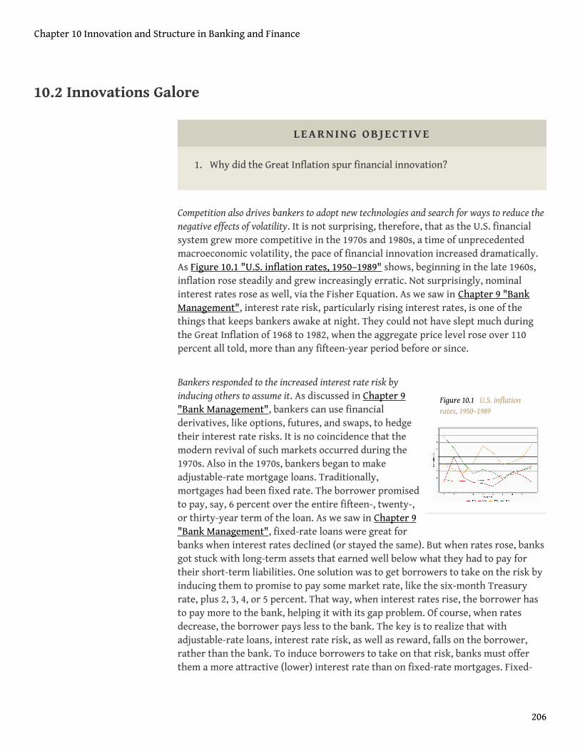
Figure 10.1 U.S. inflationrates, 1950–1989
10.2 Innovations Galore
LEARNING OBJECTIVE
1. Why did the Great Inflation spur financial innovation?
Competition also drives bankers to adopt new technologies and search for ways to reduce thenegative effects of volatility. It is not surprising, therefore, that as the U.S. financialsystem grew more competitive in the 1970s and 1980s, a time of unprecedentedmacroeconomic volatility, the pace of financial innovation increased dramatically.As Figure 10.1 "U.S. inflation rates, 1950–1989" shows, beginning in the late 1960s,inflation rose steadily and grew increasingly erratic. Not surprisingly, nominalinterest rates rose as well, via the Fisher Equation. As we saw in Chapter 9 "BankManagement", interest rate risk, particularly rising interest rates, is one of thethings that keeps bankers awake at night. They could not have slept much duringthe Great Inflation of 1968 to 1982, when the aggregate price level rose over 110percent all told, more than any fifteen-year period before or since.
Bankers responded to the increased interest rate risk byinducing others to assume it. As discussed in Chapter 9"Bank Management", bankers can use financialderivatives, like options, futures, and swaps, to hedgetheir interest rate risks. It is no coincidence that themodern revival of such markets occurred during the1970s. Also in the 1970s, bankers began to makeadjustable-rate mortgage loans. Traditionally,mortgages had been fixed rate. The borrower promisedto pay, say, 6 percent over the entire fifteen-, twenty-,or thirty-year term of the loan. As we saw in Chapter 9"Bank Management", fixed-rate loans were great forbanks when interest rates declined (or stayed the same). But when rates rose, banksgot stuck with long-term assets that earned well below what they had to pay fortheir short-term liabilities. One solution was to get borrowers to take on the risk byinducing them to promise to pay some market rate, like the six-month Treasuryrate, plus 2, 3, 4, or 5 percent. That way, when interest rates rise, the borrower hasto pay more to the bank, helping it with its gap problem. Of course, when ratesdecrease, the borrower pays less to the bank. The key is to realize that withadjustable-rate loans, interest rate risk, as well as reward, falls on the borrower,rather than the bank. To induce borrowers to take on that risk, banks must offerthem a more attractive (lower) interest rate than on fixed-rate mortgages. Fixed-
Chapter 10 Innovation and Structure in Banking and Finance
206
rate mortgages remain popular, however, because many people don’t like the riskof possibly paying higher rates in the future. Furthermore, if their mortgagescontain no prepayment penalty clause (and most don’t), borrowers know that theycan take advantage of lower interest rates by refinancing—getting a new loan at thecurrent, lower rate and using the proceeds to pay off the higher-rate loan. Due tothe high transaction costs (“closing costs” like loan application fees, appraisal costs,title insurance, and so forth) associated with home mortgage re-fis, however,interest rates must decline more than a little bit before it is worthwhile to doone.http://www.bankrate.com/brm/calc_vml/refi/refi.asp
Stop and Think Box
In the 1970s and 1980s, life insurance companies sought regulatory approval fora number of innovations, including adjustable-rate policy loans and variableannuities. Why? Hint: Policy loans are loans that whole life insurancepolicyholders can take out against the cash value of their policies. Most policiesstipulated a 5 or 6 percent fixed rate. Annuities, annual payments made duringthe life of the annuitant, were also traditionally fixed.
Life insurance companies, like banks, were adversely affected bydisintermediation during the Great Inflation. Policyholders astutely borrowedthe cash values of their life insurance policies at 5 or 6 percent, then re-lent themoney at the going market rate, which was often in the double digits. Bymaking the policy loans variable, life insurers could adjust them upward whenrates increased to limit such arbitrage. Similarly, fixed annuities were adifficult sell during the Great Inflation because annuitants saw the real value(the purchasing power) of their annual payments decrease dramatically. Bypromising to pay annuitants more when interest rates and inflation were high,variable-rate annuities helped insurers to attract customers.
Chapter 10 Innovation and Structure in Banking and Finance
10.2 Innovations Galore 207
KEY TAKEAWAYS
• By increasing macroeconomic instability, nominal interest rates, andcompetition between banks and financial markets, the Great Inflationforced bankers and other financiers to innovate.
• Bankers innovated by introducing new products, like adjustable-ratemortgages and sweep accounts; new techniques, like derivatives andother off-balance-sheet activities; and new technologies, includingcredit card payment systems and automated and online bankingfacilities.
Chapter 10 Innovation and Structure in Banking and Finance
10.2 Innovations Galore 208
10.3 Loophole Mining and Lobbying
LEARNING OBJECTIVE
1. What are loophole mining and lobbying, and why are they important?
Competition for profits also drives bankers and other financiers to look for regulatoryloopholes, a process sometimes called loophole mining. Loophole mining works better innations, like the United States, with a permissive regulatory system1 rather than arestrictive one, or, in other words, in places where anything is allowed unless it isexplicitly forbidden.Doug Arner, Financial Stability, Economic Growth, and the Role ofLaw (New York: Cambridge University Press, 2007), 263. During the Great Inflation,banks could not legally pay any interest on checking deposits or more than about 6percent on time deposits, both far less than going market rates. Banks tried to luredepositors by giving them toasters and other gifts, attempting desperately to skirtthe interest rate caps by sweetening the pot. Few depositors bit. Massivedisintermediation2 ensued because depositors pulled their money out of banks tobuy assets that could provide a market rate of return. Financiers responded bydeveloping money market mutual funds (MMMFs), which offered checkingaccount–like liquidity while paying interest at market rates, and by investing inshort-term, high-grade assets like Treasury Bills and AAA-rated corporatecommercial paper. (The growth of MMMFs in turn aided the growth anddevelopment of the commercial paper markets.)
1. A system that allows financiersto engage in any activities theywish that are not explicitlyforbidden. It is easier forfinancial innovation than arestrictive regulatory system.
2. The opposite ofintermediation, when investorspull money out of banks andother financial intermediaries.
Chapter 10 Innovation and Structure in Banking and Finance
209
Stop and Think Box
To work around regulations against interstate banking, some banks,particularly in markets that transcended state lines, established so-callednonbank banks. Because the law defined banks as institutions that “acceptdeposits and make loans,” banks surmised, correctly, that they could establishde facto branches that did one function or the other, but not both. What is thistype of behavior called and why is it important?
This is loophole mining leading to financial innovation. Unfortunately, thisparticular innovation was much less economically efficient than establishingreal branches would have been. The banks that created nonbank banks likelyprofited, but not as much as they would have if they had not had to resort tosuch a technicality. Moreover, the nonbank bank’s customers would have beenless inconvenienced!
Bankers also used loophole mining by creating so-called sweep accounts, checking accountsthat were invested each night in overnight loans. The interest earned on those loans wascredited to the account the next morning, allowing banks to pay rates above theofficial deposit rate ceilings. Sweep accounts also allowed banks to do the endaround on reserve requirements, legal minimums of cash and Federal Reservedeposits. Recall that banks earn no interest on reserves, so they often wish thatthey could hold fewer reserves than regulators require, particularly when interestrates are high. By using computers to sweep checking accounts at the close of business eachday, banks reduced their de jure deposits and thus their reserve requirements to the pointthat reserve regulations today are largely moot, a point to which we shall return.
Bank holding companies (BHCs), parent companies that own multiple banks andbanking-related service companies, offered bankers another way to use loopholemining because regulation of BHCs was, for a long time, more liberal than unit bankregulation. In particular, BHCs could circumvent restrictive branching regulationsand earn extra profits by providing investment advice, data processing, and creditcard services. Today, bank holding companies own almost all of the big U.S. banks.J.P. Morgan Chase, Bank of America, and Citigroup are allBHCs.http://www.ffiec.gov/nicpubweb/nicweb/top50form.aspx
Not all regulations can be circumvented cost effectively via loophole mining,however, so sometimes bankers and other financiers have to push for regulatoryreforms. The Great Inflation and the decline of traditional banking, we’ll learn
Chapter 10 Innovation and Structure in Banking and Finance
10.3 Loophole Mining and Lobbying 210
below, induced bankers to lobby to change the regulatory regime they faced. Thebankers largely succeeded, as we’ll see, aided in part by a banking crisis.
KEY TAKEAWAYS
• Loophole mining is a type of innovation where bankers and otherfinanciers look for creative ways of circumventing regulations.
• Lobbying is a type of innovation where bankers and other financiers tryto change regulations.
• The Great Inflation also induced bankers to use loophole mining (forexample, by using bank holding companies). When that was too costly,bankers lobbied to change the regulatory system, generally to make itless restrictive.
Chapter 10 Innovation and Structure in Banking and Finance
10.3 Loophole Mining and Lobbying 211
10.4 Banking on Technology
LEARNING OBJECTIVE
1. How has technology aided financial innovation?
Proliferation of the telegraph and the telephone in the nineteenth century did littleto change banking. Bankers in remote places could place orders with securitiesbrokers more quickly and cheaply than before, customers could perform certainlimited transactions by talking with a teller by phone rather than in person, andmechanical computers made certain types of data storage and number crunchingfaster. The widespread use of automobiles led to the adoption of drive-up tellerwindows in the 1950s. None of those technologies, however, transformed the face ofthe business. The advent of cheap electronic computing and digital telecommunicationsafter World War II, however, did eventually spur significant innovation.
Retail-level credit has always been a major component of the American economy,but it began to get crimped in the late nineteenth and early twentieth centuries inlarge urban areas where people no longer knew their neighbors and clerks left fornew jobs with alarming frequency. Some stores began to issue credit cards to theircustomers. These credit cards were literally identification cards that let the clerksknow that the customer had a credit account with the store. The system wasinefficient because consumers needed a different card for each store in which theyshopped. Moreover, as we learned in Chapter 8 "Financial Structure, TransactionCosts, and Asymmetric Information", screening good borrowers from bad isn’t easyand minimum efficient scale is quite high, so even large department store chainswere not very efficient at issuing the cards. Observers realized that economies ofscale could be exploited if one company decided who was creditworthy andprovided a payment system that allowed participation by a large percentage ofretailers.
After World War II, Diners Club applied the idea to restaurants, essentially tellingrestaurateurs that it would pay their customers’ bills. (Diners Club later collectedfrom the customers.) The service was very costly, however, so new credit cardsystems did not spread successfully until the late 1960s, when improvements incomputer technology and telecommunications made it possible for machines to conduct thetransactions at both the point of sale and card issuer sides of the transaction. Since then,several major credit card networks have arisen, and thousands of institutions,including many nonbanks, now issue credit cards.
Chapter 10 Innovation and Structure in Banking and Finance
212
Basically, Visa and MasterCard have created private payment systems that are win-win-win.Retailers win because they are assured of getting paid (checks sometimes bouncedays after the fact, but credit and debit cards can be verified before goods are givenor services are rendered). Retailers pay a small fixed fee (that’s why a shopkeepermight not let you charge a 25 cent pack of gum) and a few percentage points foreach transaction because they believe that their customers like to pay by creditcard. Indeed many do. Carrying a credit card is much easier and safer than carryingaround cash. By law, cardholders are liable for no more than $50 if their card is lostor stolen, provided they report it in a timely manner. Credit cards are small andlight, especially compared to large sums of cash, and they eliminate the need forsmall change. They also allow consumers to smooth their consumption over time byallowing them to tap a line of credit on demand. Although interest rates on creditcards are generally high, the cardholder can avoid interest charges by paying thebill in full each month. Finally, banks and other card issuers win because of the feesthey receive from vendors. Some also charge cardholders an annual fee.Competition, however, has largely ended the annual fee card and indeed drivenissuers to refund some of the fees they collect from retailers to cardholders toinduce people to pay with their cards rather than with cash, check, or competitors’cards. That’s what all of the business about cash back, rewards, frequent flierpoints, and the like, is about.
Debit cards look like credit cards but actually tap into the cardholder’s checkingaccount much like an instantaneous check. Retailers like them better than checks,though, because a debit card can’t bounce, or be returned for insufficient fundsdays after the customer has walked off with the store owner’s property. Consumerswho find it difficult to control their spending find debit cards useful because it givesthem firm budget constraints, that is, the sums in their respective checkingaccounts. If a debit card is lost or stolen, however, the cardholder’s liability isgenerally much higher than it is with a credit card. Today, many debit cards arealso automatic teller machine (ATM) cards, cards that allow customers to withdrawcash from ATMs. That makes sense because, like debit cards, ATM cards are linkeddirectly to each cardholder’s checking (and sometimes savings) accounts. ATMs aremuch smaller, cheaper, and more convenient than full-service branches, so many banksestablished networks of them instead of branches. Before bank branching restrictionswere lifted, ATMs also received more favorable regulatory treatment thanbranches. There are more than 250,000 ATMs in the United States today, all linkedto bank databases via the miraculous telecom devices developed in the latetwentieth century.
Chapter 10 Innovation and Structure in Banking and Finance
10.4 Banking on Technology 213
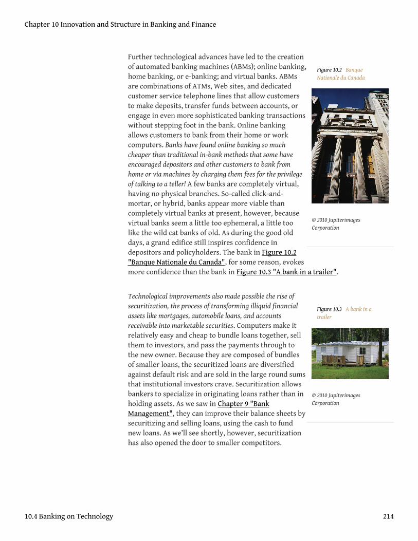
Figure 10.2 BanqueNationale du Canada
© 2010 JupiterimagesCorporation
Figure 10.3 A bank in atrailer
© 2010 JupiterimagesCorporation
Further technological advances have led to the creationof automated banking machines (ABMs); online banking,home banking, or e-banking; and virtual banks. ABMsare combinations of ATMs, Web sites, and dedicatedcustomer service telephone lines that allow customersto make deposits, transfer funds between accounts, orengage in even more sophisticated banking transactionswithout stepping foot in the bank. Online bankingallows customers to bank from their home or workcomputers. Banks have found online banking so muchcheaper than traditional in-bank methods that some haveencouraged depositors and other customers to bank fromhome or via machines by charging them fees for the privilegeof talking to a teller! A few banks are completely virtual,having no physical branches. So-called click-and-mortar, or hybrid, banks appear more viable thancompletely virtual banks at present, however, becausevirtual banks seem a little too ephemeral, a little toolike the wild cat banks of old. As during the good olddays, a grand edifice still inspires confidence indepositors and policyholders. The bank in Figure 10.2"Banque Nationale du Canada", for some reason, evokesmore confidence than the bank in Figure 10.3 "A bank in a trailer".
Technological improvements also made possible the rise ofsecuritization, the process of transforming illiquid financialassets like mortgages, automobile loans, and accountsreceivable into marketable securities. Computers make itrelatively easy and cheap to bundle loans together, sellthem to investors, and pass the payments through tothe new owner. Because they are composed of bundlesof smaller loans, the securitized loans are diversifiedagainst default risk and are sold in the large round sumsthat institutional investors crave. Securitization allowsbankers to specialize in originating loans rather than inholding assets. As we saw in Chapter 9 "BankManagement", they can improve their balance sheets bysecuritizing and selling loans, using the cash to fundnew loans. As we’ll see shortly, however, securitizationhas also opened the door to smaller competitors.
Chapter 10 Innovation and Structure in Banking and Finance
10.4 Banking on Technology 214
KEY TAKEAWAYS
• Technology, particularly digital electronic computers andtelecommunication devices, made possible sweep accounts,securitization, credit and debit card networks, ATMs, ABMs, and onlinebanking.
• ATMs, ABMs, and online banking reduced a bank’s expenses.• Sweep accounts reduced the cost of required reserves.• Securitization allows banks to specialize in making loans, as opposed to
holding assets.• Credit card issuance is often lucrative.
Chapter 10 Innovation and Structure in Banking and Finance
10.4 Banking on Technology 215
10.5 Banking Industry Profitability and Structure
LEARNING OBJECTIVE
1. What role does market structure (concentration, consolidation,conglomeration) play in the banking industry’s profitability?
Despite their best innovation efforts, banks have been steadily losing market shareas sources of loans to nonfinancial borrowers. In the 1970s, commercial banks andother depository institutions (the so-called thrifts—credit unions, savings andloans, savings banks) controlled over 60 percent of that market. Today, they haveonly about a third. The market for loans to nonfinancial borrowers grew veryquickly over the last quarter century, however, so that decline is a relative oneonly. Banks are still extremely profitable, so much so that many new banks formeach year. But bankers have to work harder than ever for those profits; the good old days oftraditional banking and the 3-6-3 rule are long gone. Fees and other off-balance-sheetactivities now account for almost half of bank income, up from about 7 percent in1980. The traditional source of profit, the spread between the cost of liabilities andthe returns on assets, has steadily eroded from both ends.
As noted above, the interest rates that banks could pay on deposits were capped(under so-called Regulation Q) at 0 for checking deposits and about 6 percent ontime deposits. Until the Great Inflation, bankers loved the caps because they limitedcompetition for deposits. When interest rates rose enough to causedisintermediation, to cause funds to flow out of banks to higher-yieldinginvestments like money market mutual funds, bankers lobbied for an end to theinterest rate restrictions and their request was granted in the 1980s. Since then,banks have had to compete with each other as well as with money market mutualfunds for deposits. Unsurprisingly, banks have to pay more for deposits than ever before(the general level of interest rates constant). Little wonder that deposits have becomerelatively less important as sources of funds for banks.
On the asset side, banks can’t charge as much for loans, ceteris paribus, as they once didbecause they face increasingly stiff competition from the commercial paper and bondmarkets, especially the so-called junk bond market. Now, instead of having to cozy up toa bank, smaller and riskier companies can sell bonds directly to investors. Issuingbonds incurs costs besides interest charges—namely, mandatory informationdisclosure and constant feedback from investors on the issuing firm’s performance
Chapter 10 Innovation and Structure in Banking and Finance
216
via its bond prices—but companies are willing to bear those costs if they can get abetter interest rate than banks offer.
As mentioned above, securitization has also hurt banks by giving rise to numerous smalllenders that basically sell every loan they originate. Such companies can be efficient atsmaller scale because they do not have to attract and retain deposits or engage inmore sophisticated asset and liability management techniques. All they have to dois originate loans and sell them to investors, using the proceeds to make new loans.Finance companies especially have eaten into banks’ market share in commerciallending, and a slew of specialized mortgage lenders made major inroads into thehome mortgage market. What is good for the goose, as they say, is good for thegander.http://www.bartleby.com/59/3/whatsgoodfor.html
As a result of those competitive pressures, many banks exited the business, some by goingbankrupt, others by merging with larger institutions. The banking crisis of the 1980senabled bankers and regulators to make further reforms, including greatly easingrestrictions on branch banking and investment banking (securities) activities. In1933, at the nadir of the Great Depression, commercial and investment bankingactivities, receiving deposits and making loans and underwriting securitiesofferings, respectively, were strictly separated by legislation usually called Glass-Steagall, after the congressional members who cooked it up. The gradual de factoerosion of Glass-Steagall in the late 1980s and 1990s (by means of bank holdingcompanies and a sympathetic Federal Reserve) and its de jure elimination in 1999allowed investment and commercial banks to merge and to engage in each other’sactivities. Due to those and other regulatory changes, usually called deregulation,and the decline of traditional banking, banks began to merge in large numbers, aprocess called consolidation, and began to enter into nonbanking financialactivities, like insurance, a process called conglomeration.
As Figure 10.4 "Number of FDIC commercial banks, year-end, 1980–2010" and Figure10.5 "U.S. banks: return on equity, 1935–2010" show, consolidation and conglomerationhave left the nation with fewer but larger and more profitable (and ostensibly more efficient)banks. Due to the demise of Glass-Steagall, conglomerate banks can now more easilytap economies of scope, the ability to use a single resource to supply numerousproducts or services. For example, banks can now use the information they createabout borrowers to offer loans or securities underwriting and can use branches toschlep insurance. Consolidation has also allowed banks to diversify their risksgeographically and to tap economies of scale. That is important because minimumefficient scale may have increased in recent decades due to the high initial costs ofemploying the latest and greatest computer and telecommunications technologies.
Chapter 10 Innovation and Structure in Banking and Finance
10.5 Banking Industry Profitability and Structure 217
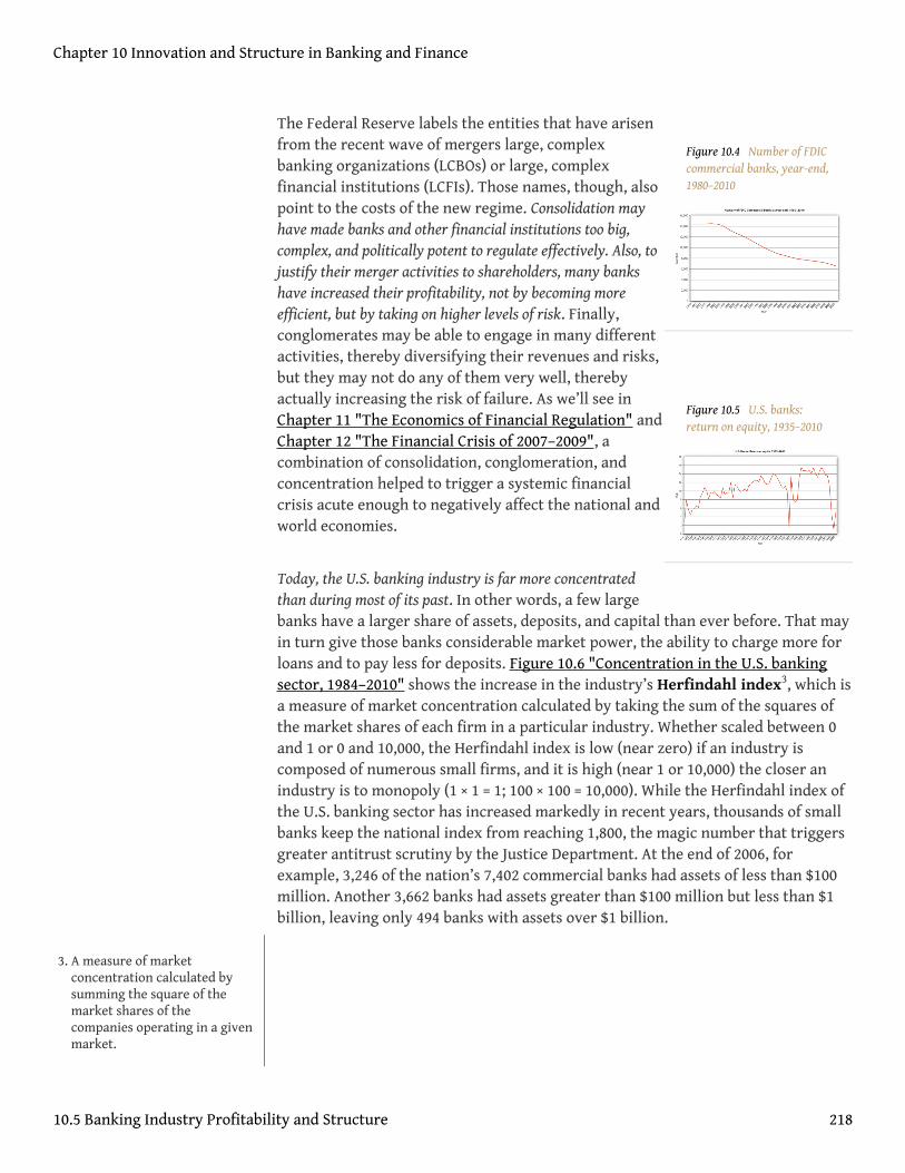
Figure 10.4 Number of FDICcommercial banks, year-end,1980–2010
Figure 10.5 U.S. banks:return on equity, 1935–2010
The Federal Reserve labels the entities that have arisenfrom the recent wave of mergers large, complexbanking organizations (LCBOs) or large, complexfinancial institutions (LCFIs). Those names, though, alsopoint to the costs of the new regime. Consolidation mayhave made banks and other financial institutions too big,complex, and politically potent to regulate effectively. Also, tojustify their merger activities to shareholders, many bankshave increased their profitability, not by becoming moreefficient, but by taking on higher levels of risk. Finally,conglomerates may be able to engage in many differentactivities, thereby diversifying their revenues and risks,but they may not do any of them very well, therebyactually increasing the risk of failure. As we’ll see inChapter 11 "The Economics of Financial Regulation" andChapter 12 "The Financial Crisis of 2007–2009", acombination of consolidation, conglomeration, andconcentration helped to trigger a systemic financialcrisis acute enough to negatively affect the national andworld economies.
Today, the U.S. banking industry is far more concentratedthan during most of its past. In other words, a few largebanks have a larger share of assets, deposits, and capital than ever before. That mayin turn give those banks considerable market power, the ability to charge more forloans and to pay less for deposits. Figure 10.6 "Concentration in the U.S. bankingsector, 1984–2010" shows the increase in the industry’s Herfindahl index3, which isa measure of market concentration calculated by taking the sum of the squares ofthe market shares of each firm in a particular industry. Whether scaled between 0and 1 or 0 and 10,000, the Herfindahl index is low (near zero) if an industry iscomposed of numerous small firms, and it is high (near 1 or 10,000) the closer anindustry is to monopoly (1 × 1 = 1; 100 × 100 = 10,000). While the Herfindahl index ofthe U.S. banking sector has increased markedly in recent years, thousands of smallbanks keep the national index from reaching 1,800, the magic number that triggersgreater antitrust scrutiny by the Justice Department. At the end of 2006, forexample, 3,246 of the nation’s 7,402 commercial banks had assets of less than $100million. Another 3,662 banks had assets greater than $100 million but less than $1billion, leaving only 494 banks with assets over $1 billion.
3. A measure of marketconcentration calculated bysumming the square of themarket shares of thecompanies operating in a givenmarket.
Chapter 10 Innovation and Structure in Banking and Finance
10.5 Banking Industry Profitability and Structure 218
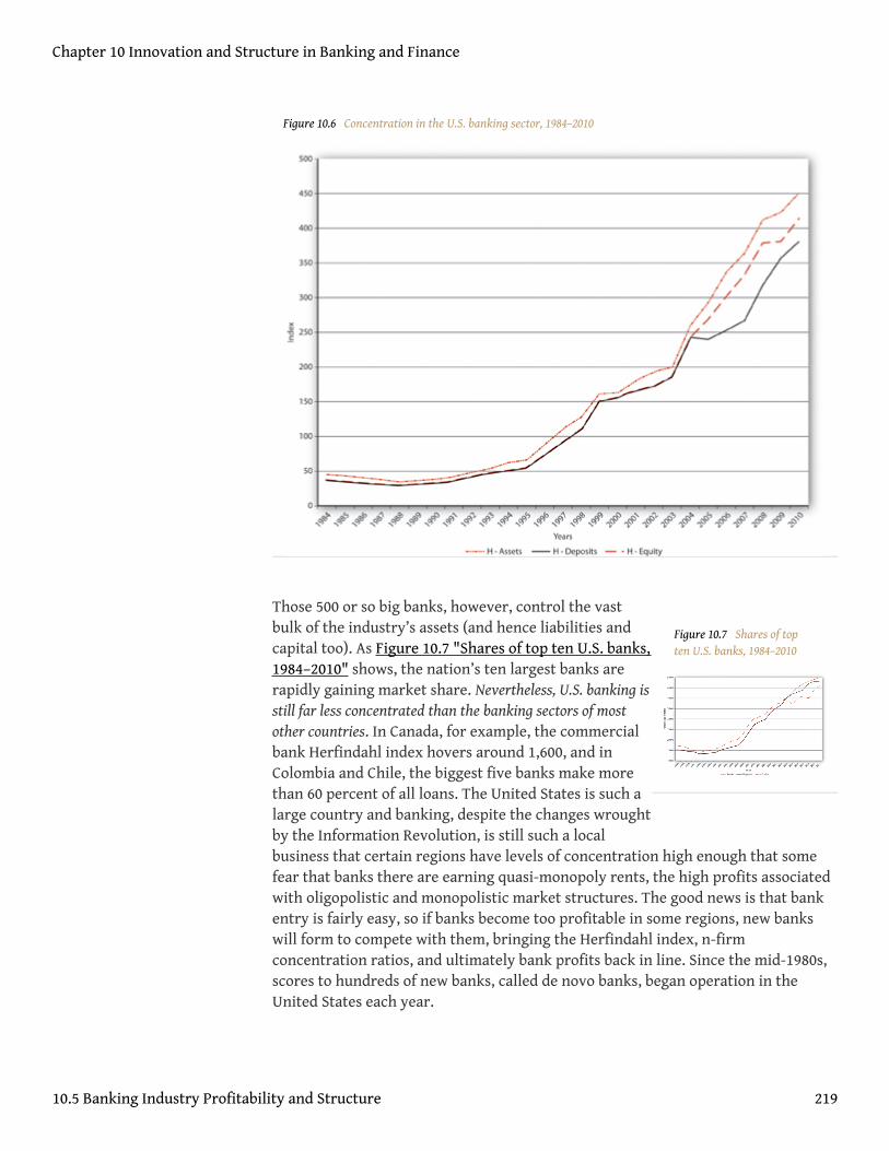
Figure 10.7 Shares of topten U.S. banks, 1984–2010
Figure 10.6 Concentration in the U.S. banking sector, 1984–2010
Those 500 or so big banks, however, control the vastbulk of the industry’s assets (and hence liabilities andcapital too). As Figure 10.7 "Shares of top ten U.S. banks,1984–2010" shows, the nation’s ten largest banks arerapidly gaining market share. Nevertheless, U.S. banking isstill far less concentrated than the banking sectors of mostother countries. In Canada, for example, the commercialbank Herfindahl index hovers around 1,600, and inColombia and Chile, the biggest five banks make morethan 60 percent of all loans. The United States is such alarge country and banking, despite the changes wroughtby the Information Revolution, is still such a localbusiness that certain regions have levels of concentration high enough that somefear that banks there are earning quasi-monopoly rents, the high profits associatedwith oligopolistic and monopolistic market structures. The good news is that bankentry is fairly easy, so if banks become too profitable in some regions, new bankswill form to compete with them, bringing the Herfindahl index, n-firmconcentration ratios, and ultimately bank profits back in line. Since the mid-1980s,scores to hundreds of new banks, called de novo banks, began operation in theUnited States each year.
Chapter 10 Innovation and Structure in Banking and Finance
10.5 Banking Industry Profitability and Structure 219
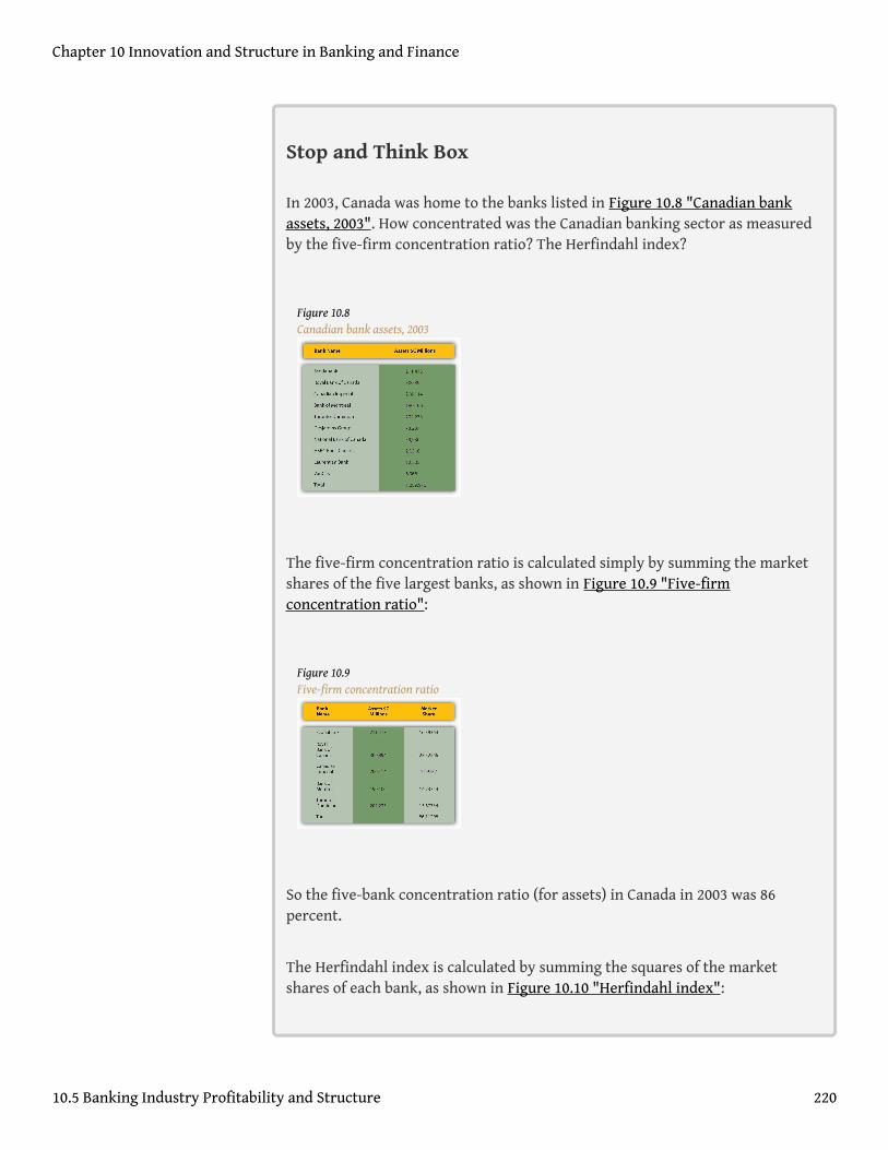
Stop and Think Box
In 2003, Canada was home to the banks listed in Figure 10.8 "Canadian bankassets, 2003". How concentrated was the Canadian banking sector as measuredby the five-firm concentration ratio? The Herfindahl index?
Figure 10.8Canadian bank assets, 2003
The five-firm concentration ratio is calculated simply by summing the marketshares of the five largest banks, as shown in Figure 10.9 "Five-firmconcentration ratio":
Figure 10.9Five-firm concentration ratio
So the five-bank concentration ratio (for assets) in Canada in 2003 was 86percent.
The Herfindahl index is calculated by summing the squares of the marketshares of each bank, as shown in Figure 10.10 "Herfindahl index":
Chapter 10 Innovation and Structure in Banking and Finance
10.5 Banking Industry Profitability and Structure 220
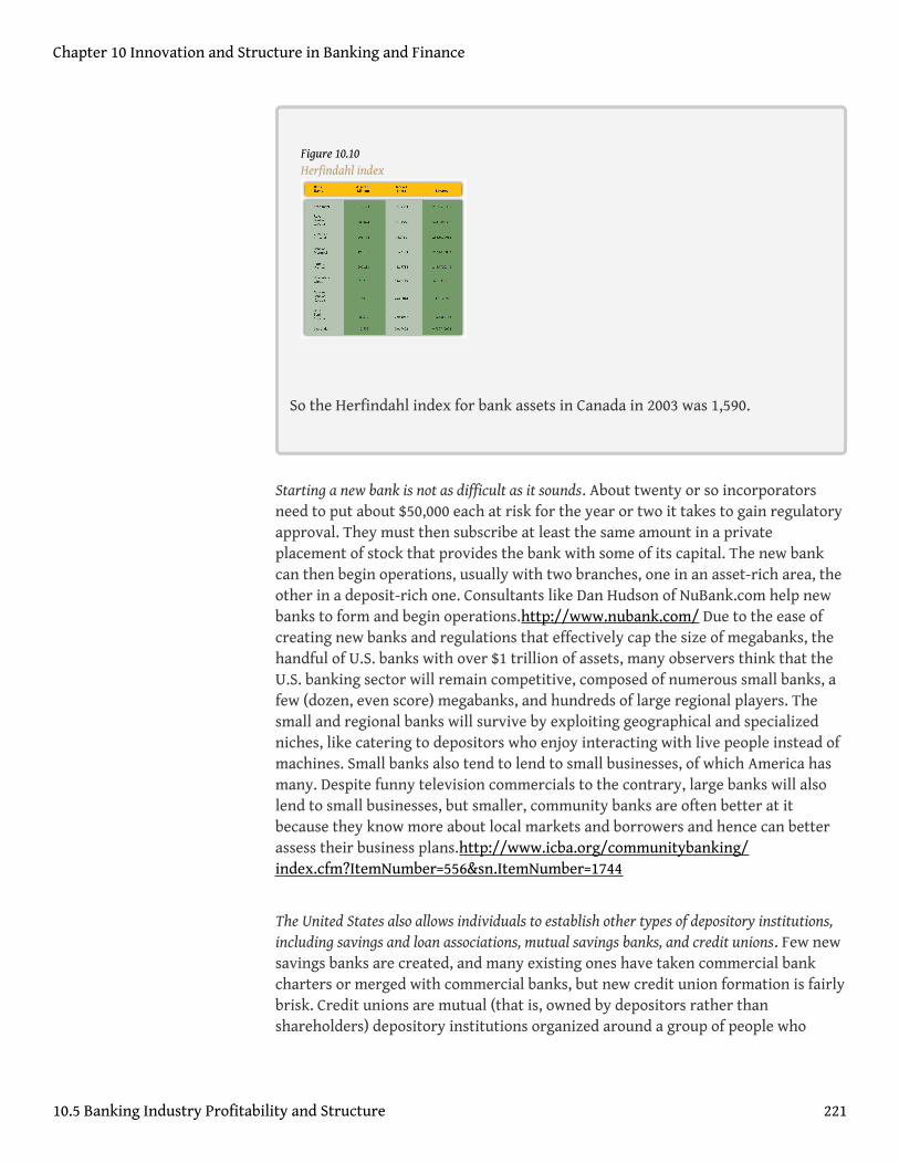
Figure 10.10Herfindahl index
So the Herfindahl index for bank assets in Canada in 2003 was 1,590.
Starting a new bank is not as difficult as it sounds. About twenty or so incorporatorsneed to put about $50,000 each at risk for the year or two it takes to gain regulatoryapproval. They must then subscribe at least the same amount in a privateplacement of stock that provides the bank with some of its capital. The new bankcan then begin operations, usually with two branches, one in an asset-rich area, theother in a deposit-rich one. Consultants like Dan Hudson of NuBank.com help newbanks to form and begin operations.http://www.nubank.com/ Due to the ease ofcreating new banks and regulations that effectively cap the size of megabanks, thehandful of U.S. banks with over $1 trillion of assets, many observers think that theU.S. banking sector will remain competitive, composed of numerous small banks, afew (dozen, even score) megabanks, and hundreds of large regional players. Thesmall and regional banks will survive by exploiting geographical and specializedniches, like catering to depositors who enjoy interacting with live people instead ofmachines. Small banks also tend to lend to small businesses, of which America hasmany. Despite funny television commercials to the contrary, large banks will alsolend to small businesses, but smaller, community banks are often better at itbecause they know more about local markets and borrowers and hence can betterassess their business plans.http://www.icba.org/communitybanking/index.cfm?ItemNumber=556&sn.ItemNumber=1744
The United States also allows individuals to establish other types of depository institutions,including savings and loan associations, mutual savings banks, and credit unions. Few newsavings banks are created, and many existing ones have taken commercial bankcharters or merged with commercial banks, but new credit union formation is fairlybrisk. Credit unions are mutual (that is, owned by depositors rather thanshareholders) depository institutions organized around a group of people who
Chapter 10 Innovation and Structure in Banking and Finance
10.5 Banking Industry Profitability and Structure 221
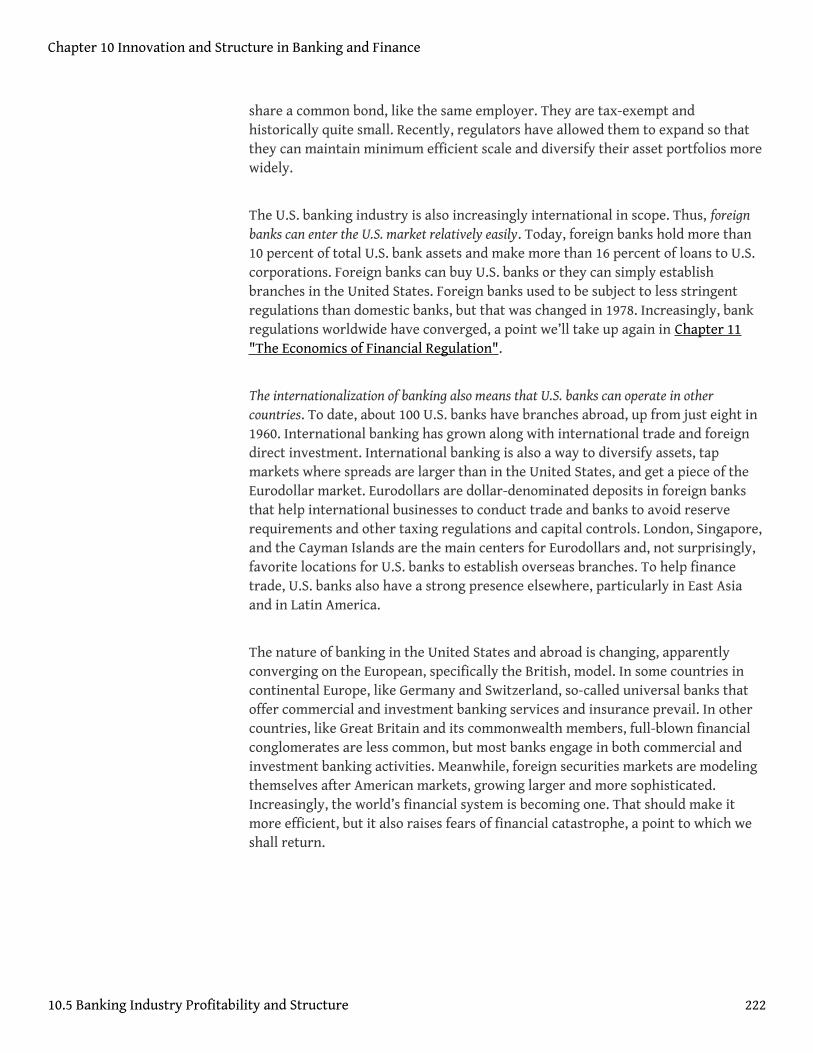
share a common bond, like the same employer. They are tax-exempt andhistorically quite small. Recently, regulators have allowed them to expand so thatthey can maintain minimum efficient scale and diversify their asset portfolios morewidely.
The U.S. banking industry is also increasingly international in scope. Thus, foreignbanks can enter the U.S. market relatively easily. Today, foreign banks hold more than10 percent of total U.S. bank assets and make more than 16 percent of loans to U.S.corporations. Foreign banks can buy U.S. banks or they can simply establishbranches in the United States. Foreign banks used to be subject to less stringentregulations than domestic banks, but that was changed in 1978. Increasingly, bankregulations worldwide have converged, a point we’ll take up again in Chapter 11"The Economics of Financial Regulation".
The internationalization of banking also means that U.S. banks can operate in othercountries. To date, about 100 U.S. banks have branches abroad, up from just eight in1960. International banking has grown along with international trade and foreigndirect investment. International banking is also a way to diversify assets, tapmarkets where spreads are larger than in the United States, and get a piece of theEurodollar market. Eurodollars are dollar-denominated deposits in foreign banksthat help international businesses to conduct trade and banks to avoid reserverequirements and other taxing regulations and capital controls. London, Singapore,and the Cayman Islands are the main centers for Eurodollars and, not surprisingly,favorite locations for U.S. banks to establish overseas branches. To help financetrade, U.S. banks also have a strong presence elsewhere, particularly in East Asiaand in Latin America.
The nature of banking in the United States and abroad is changing, apparentlyconverging on the European, specifically the British, model. In some countries incontinental Europe, like Germany and Switzerland, so-called universal banks thatoffer commercial and investment banking services and insurance prevail. In othercountries, like Great Britain and its commonwealth members, full-blown financialconglomerates are less common, but most banks engage in both commercial andinvestment banking activities. Meanwhile, foreign securities markets are modelingthemselves after American markets, growing larger and more sophisticated.Increasingly, the world’s financial system is becoming one. That should make itmore efficient, but it also raises fears of financial catastrophe, a point to which weshall return.
Chapter 10 Innovation and Structure in Banking and Finance
10.5 Banking Industry Profitability and Structure 222
KEY TAKEAWAYS
• Industry consolidation is measured by the number of banks in existenceat a given time.
• As the number of banks declines (because mergers and bankruptciesexceed new bank formation), the industry is said to become moreconsolidated. It is important because a more consolidated industry maybe safer and more profitable as smaller, weaker institutions areswallowed up by larger, stronger ones.
• However, consolidation can also lead to higher costs for consumers andborrowers and poorer service.
• Bigger banks are likely to be more diversified than smaller ones, butthey might also take on higher levels of risk, thereby threatening thestability of the financial system.
• Conglomeration refers to the scope of activities that a bank or otherfinancial intermediary is allowed to engage in.
• Traditionally, U.S. banks could engage in commercial banking activitiesor investment banking activities, but not both, and they could not sell orunderwrite insurance. Due to recent regulatory changes, however,banks and other financial intermediaries and facilitators like brokeragescan now merge into the same company or exist under the same holdingcompany umbrella.
• This deregulation may increase competition for financialintermediaries, thereby driving innovation. It could also lead, however,to the creation of financial conglomerates that are too large andcomplex to regulate adequately.
• Industry concentration is a proxy for competition and is measured bythe n-firm concentration of assets (revenues, capital, etc., where n is 1,3, 5, 10, 25, 50, etc.) or by the Herfindahl index, the sum of the square ofthe market shares (again for assets, deposits, revenues, capital, etc.) ofeach company in the industry or in a given city, state, or region.
• Concentration is important because a highly concentrated industry maybe less competitive, leading to less innovation, higher costs forborrowers, outsized profits for suppliers (in this case banks), and a morefragile (prone to systemic crisis) banking system.
• On the other hand, as banking has grown more concentrated, individualbanks have become more geographically diversified, which may helpthem to better weather economic downturns.
Chapter 10 Innovation and Structure in Banking and Finance
10.5 Banking Industry Profitability and Structure 223
10.6 Suggested Reading
Anderloni, Luisa, David Llewellyn, and Reinhard Schmidt. Financial Innovation inRetail and Corporate Banking. Northampton, MA: Edward Elgar, 2009.
Banner, Stuart. Anglo-American Securities Regulation: Cultural and Political Roots,1690–1860. New York: Cambridge University Press, 2002.
Freedman, Roy. Introduction to Financial Technology. New York: Academic Press, 2006.
Shiller, Robert. The New Financial Order: Risk in the 21st Century. Princeton, NJ:Princeton University Press, 2004.
Wright, Robert E. The Wealth of Nations Rediscovered: Integration and Expansion inAmerican Financial Markets, 1780–1850. New York: Cambridge University Press, 2002.
Wright, Robert E., and David J. Cowen. Financial Founding Fathers: The Men Who MadeAmerica Rich. Chicago, IL: Chicago University Press, 2006.
Wright, Robert E., and George D. Smith. Mutually Beneficial: The Guardian and LifeInsurance in America. New York: New York University Press, 2004.
Chapter 10 Innovation and Structure in Banking and Finance
224
Chapter 11
The Economics of Financial Regulation
CHAPTER OBJECTIVES
By the end of this chapter, students should be able to:
1. Explain why the government can’t simply legislate bad things out ofexistence.
2. Describe the public interest and private interest models of governmentand explain why they are important.
3. Explain how asymmetric information interferes with regulatory efforts.4. Describe how government regulators exacerbated the Great Depression.5. Describe how government regulators made the Savings and Loan Crisis
worse.6. Assess recent regulatory reforms in the United States and both Basel
accords.
225
11.1 Public Interest versus Private Interest
LEARNING OBJECTIVE
1. Why can’t the government legislate bad things out of existence andwhich model of government, public interest or private interest, is themost accurate depiction of reality?
Whenever anything seemingly bad happens in the world, many people todayimmediately clamor for the government to do something about it. That issometimes an appropriate response, but many times it is not. For starters,government can’t fix the world by decree. Simply making an activity illegal does not meanthat it will stop. Because the government faces a budget constraint and opportunitycosts, it can’t afford to monitor everyone all the time. What’s bad for some is oftengood for others, so many people willingly supply illegal goods or activities. As aresult, many illegal activities are commonplace; in no particular order, sodomy,drug use, reckless use of automobiles, and music piracy come to mind.
The second problem with relying on government to fix bad things is that governmentofficials are not the angels many people assume they are. It’s not your fault. Especially ifyou went through the U.S. public school system, you likely learned aninterpretation of government called the public interest model. As its name suggests,the public interest model1posits that government officials work in the interests of thepublic, of “the people,” if you will. It’s the sort of thing Abraham Lincoln had in mind inhis famous Gettysburg Address when he said “that government of the people, by thepeople, for the people, shall not perish from the earth.”http://showcase.netins.net/web/creative/lincoln/speeches/gettysburg.htm That’s outstanding politicalrhetoric, better than anything current spin artists concoct, but is it a fairrepresentation of reality?
Many economists think not. They believe that private interest prevails, even in thegovernment. According to their model, called the public choice2 or, less confusingly, theprivate interest model3, politicians and bureaucrats often behave in their own interestsrather than those of the public. Of course, they don’t go around saying that we needlaw X or regulation Y to help me to get rich via bribes, to bailout my brother-in-law,or to ensure that I soon receive a cushy job in the private sector. Rather, they saythat we need law X or regulation Y to protect widows and orphans, to stymie theefforts of bad guys, or to make the rich pay for their success.
1. A model of governmentdeveloped by politicalscientists that posits thatpoliticians, bureaucrats, andother government workersserve the public in lieu ofthemselves.
2. See private interest model.
3. A model of governmentdeveloped by economists thatposits that politicians,bureaucrats, and othergovernment workers servethemselves in lieu of thecitizens or public.
Chapter 11 The Economics of Financial Regulation
226
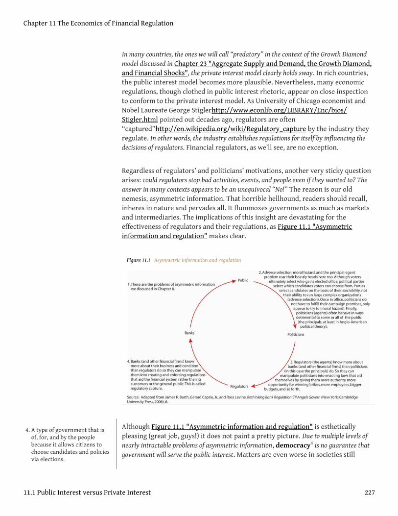
In many countries, the ones we will call “predatory” in the context of the Growth Diamondmodel discussed in Chapter 23 "Aggregate Supply and Demand, the Growth Diamond,and Financial Shocks", the private interest model clearly holds sway. In rich countries,the public interest model becomes more plausible. Nevertheless, many economicregulations, though clothed in public interest rhetoric, appear on close inspectionto conform to the private interest model. As University of Chicago economist andNobel Laureate George Stiglerhttp://www.econlib.org/LIBRARY/Enc/bios/Stigler.html pointed out decades ago, regulators are often“captured”http://en.wikipedia.org/wiki/Regulatory_capture by the industry theyregulate. In other words, the industry establishes regulations for itself by influencing thedecisions of regulators. Financial regulators, as we’ll see, are no exception.
Regardless of regulators’ and politicians’ motivations, another very sticky questionarises: could regulators stop bad activities, events, and people even if they wanted to? Theanswer in many contexts appears to be an unequivocal “No!” The reason is our oldnemesis, asymmetric information. That horrible hellhound, readers should recall,inheres in nature and pervades all. It flummoxes governments as much as marketsand intermediaries. The implications of this insight are devastating for theeffectiveness of regulators and their regulations, as Figure 11.1 "Asymmetricinformation and regulation" makes clear.
Figure 11.1 Asymmetric information and regulation
Although Figure 11.1 "Asymmetric information and regulation" is estheticallypleasing (great job, guys!) it does not paint a pretty picture. Due to multiple levels ofnearly intractable problems of asymmetric information, democracy4 is no guarantee thatgovernment will serve the public interest. Matters are even worse in societies still
4. A type of government that isof, for, and by the peoplebecause it allows citizens tochoose candidates and policiesvia elections.
Chapter 11 The Economics of Financial Regulation
11.1 Public Interest versus Private Interest 227
plagued by predatory government5, where corruption further fouls up the worksby giving politicians, regulators, and bankers (and other financiers) incentives toperpetuate the current system, no matter how suboptimal it may be from thepublic’s point of view.
And if you really want to get your head spinning, consider this: agency problems within thegovernment, within regulatory bureaucracies, and within banks abound. Within banks,traders and loan officers want to keep their jobs, earn promotions, and bring homelarge bonuses. They can do the latter two by taking large risks, and sometimes theychoose to do so. Sometimes shareholders want to take on much larger risks thanmanagers or depositors or other debt holders do. Sometimes it’s the managers whohave incentives to place big bets, to get their stock options “in themoney.”http://www.investorwords.com/2580/in_the_money.html Withinbureaucracies, regulators have incentives to hide their mistakes and to take creditfor good outcomes, even if they had little or nothing to do with them. The same istrue for the government, where the legislature may try to discredit the executive’spolicies, or vice versa, and withhold information or even spread disinformation to“prove” its case.
Stop and Think Box
In the 1910s and early 1920s, a majority of U.S. states passed securitiesregulations called Blue Sky Laws that ostensibly sought to prevent slimysecurities dealers from selling nothing but the blue sky to poor, defenselesswidows and orphans. Can you figure out what was really going on? (Hint: Recallthat this was a period of traditional banking, unit banks, the 3-6-3 rule, and allthat. Recall, too, that securities markets are an alternative method of linkinginvestors to borrowers.)
We probably gave it away with that last hint. Blue Sky Laws, scholars nowrealize, were veiled attempts to protect the monopolies of unit bankers upsetabout losing business to the securities markets. Unable to garner publicsympathy for their plight, the bankers instead spoke in terms of public interest,of defrauded widows and orphans. There were certainly some scams about, butnot enough to warrant the more virulent Blue Sky Laws, which actually gavestate officials the power to forbid issuance of securities they didn’t like, and insome states, that was most of them!
5. A type of government that isof, for, and by the ruling eliteand that fails to supply basicpublic goods like life, liberty,and property.
Chapter 11 The Economics of Financial Regulation
11.1 Public Interest versus Private Interest 228
It’s okay if you feel a bit uneasy with these new ideas. We think that as adults youcan handle straight talk. It’ll be better for everyone—you, me, our children andgrandchildren—if you learn to look at the government’s actions with a jaundicedeye. Regulators have failed in the past and will do so again unless we align the interests ofall the major parties depicted in Figure 11.1 "Asymmetric information and regulation"more closely, empowering market forces to do most of the heavy lifting.
KEY TAKEAWAYS
• The government can’t legislate bad things away because it can’t be everyplace at once. Like the rest of us, government faces budget constraintsand opportunity costs. Therefore, it cannot stop activities that somepeople enjoy or find profitable.
• According to the public interest model, government tries to enact laws,regulations, and policies that benefit the public.
• The private interest (or public choice) model, by contrast, suggests thatgovernment officials enact laws that are in their own private interest.
• It is important to know which model is a more accurate description ofreality because the models have very different implications for ourattitudes toward regulation.
• If one believes the public interest model is usually correct, then one willbe more likely to call for government regulation, even if one admits thatregulatory goals may in fact be difficult to achieve regardless of theintentions of politicians and bureaucrats.
• If one believes the private interest model is a more accurate depiction ofthe real world, one will be more skeptical of government regulation.
• Asymmetric information creates a principal-agent problem between thepublic and elected officials, another principal-agent problem betweenthose officials and regulators, and yet another principal-agent problembetween regulators and banks (and other financial firms) because ineach case, one party (politicians, regulators, banks) knows more thanthe other (public, politicians, regulators).
• So there are at least three places where the public’s interest can bestymied: in political elections, in the interaction between Congress andthe president and regulatory agencies, and in the interaction betweenregulators and the regulated. And that’s ignoring the often extensiveagency problems found within governments, regulatory agencies, andfinancial institutions!
Chapter 11 The Economics of Financial Regulation
11.1 Public Interest versus Private Interest 229
11.2 The Great Depression as Regulatory Failure
LEARNING OBJECTIVE
1. How did the government exacerbate the Great Depression?
Time again, government regulators have either failed to stop financial crises or haveexacerbated them. Examples are too numerous to discuss in detail here, so we willaddress only two of the more egregious cases, the Great Depression of the 1930s andthe Savings and Loan (S&L) Crisis of the 1980s.
Generally when economic matters go FUBAR (Fouled Up Beyond All Recognition inpolite circles), observers blame either “market failures” like asymmetricinformation and externalities6, or they blame the government. Reality is rarelythat simple. Most major economic foul-ups stem from a combination of market andgovernment failures, what we like to call hybrid failures. So while it would be anexaggeration to claim that government policies were the only causes of the GreatDepression or the Savings and Loan Crisis, it is fair to say that they made mattersworse, much worse.
Everyone knows that the stock market crash of 1929 started the Great Depression.As we will learn in Chapter 23 "Aggregate Supply and Demand, the GrowthDiamond, and Financial Shocks", a precipitous decline in stock prices can causeuncertainty to increase and balance sheets to deteriorate, worsening asymmetricinformation problems and leading to a decline in economic activity. That, in turn,can cause bank panics, further increases in asymmetric information, and yetfurther declines in economic activity followed by an unanticipated decline in theprice level. As Figure 11.2 "Major macro variables during the Great Depression"shows, that is precisely what happened during the Great Depression— per capita grossdomestic product (GDP) shrank, the number of bankruptcies soared, M1 and M2 (measures ofthe money supply) declined, and so did the price level.
6. Costs or benefits of aneconomic activity that are notincluded in the price, that arenot internalized by the buyerand/or seller. Negativeexternalities, like pollution,impose costs on society;positive externalities, likeeducation, provide societalbenefits.
Chapter 11 The Economics of Financial Regulation
230
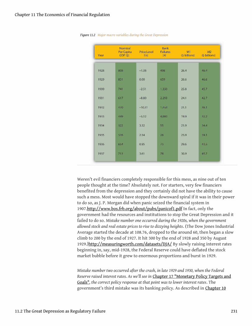
Figure 11.2 Major macro variables during the Great Depression
Weren’t evil financiers completely responsible for this mess, as nine out of tenpeople thought at the time? Absolutely not. For starters, very few financiersbenefited from the depression and they certainly did not have the ability to causesuch a mess. Most would have stopped the downward spiral if it was in their powerto do so, as J. P. Morgan did when panic seized the financial system in1907.http://www.bos.frb.org/about/pubs/panicof1.pdf In fact, only thegovernment had the resources and institutions to stop the Great Depression and itfailed to do so. Mistake number one occurred during the 1920s, when the governmentallowed stock and real estate prices to rise to dizzying heights. (The Dow Jones IndustrialAverage started the decade at 108.76, dropped to the around 60, then began a slowclimb to 200 by the end of 1927. It hit 300 by the end of 1928 and 350 by August1929.)http://measuringworth.com/datasets/DJA/ By slowly raising interest ratesbeginning in, say, mid-1928, the Federal Reserve could have deflated the stockmarket bubble before it grew to enormous proportions and burst in 1929.
Mistake number two occurred after the crash, in late 1929 and 1930, when the FederalReserve raised interest rates. As we’ll see in Chapter 17 "Monetary Policy Targets andGoals", the correct policy response at that point was to lower interest rates. Thegovernment’s third mistake was its banking policy. As described in Chapter 10
Chapter 11 The Economics of Financial Regulation
11.2 The Great Depression as Regulatory Failure 231
"Innovation and Structure in Banking and Finance", the United States was home to tensof thousands of tiny unit banks that simply were not large or diversified enough to ride outthe depression. If a factory or other major employer succumbed, the local bank toowas doomed. Depositors understood this, so at the first sign of trouble they ran ontheir banks, pulling out their deposits before they went under. Their actionsguaranteed that their banks would indeed fail. Meanwhile, across the border inCanada, which was home to a few large and highly diversified banks, few bankdisturbances took place. California also weathered the Great Depression relativelywell, in part because its banks, which freely branched throughout the large state,enjoyed relatively well-diversified assets and hence avoided the worst of the bankcrises.
The government’s fourth failure was to raise tariffs in a misguided attempt to “beggar thyneighbor.”http://www.state.gov/r/pa/ho/time/id/17606.htm Detailed analysis ofthis failure, which falls outside the bailiwick of finance, we’ll leave to yourinternational economics textbook and a case in Chapter 21 "IS-LM". Here, we’ll justparaphrase Mr. Mackey from South Park: “Tariffs are bad,mmmkay?”http://en.wikipedia.org/wiki/List_of_staff_at_South_Park_Elementary#Mr._Mackey
But what about Franklin Delano Roosevelt (FDR)http://www.whitehouse.gov/history/presidents/fr32.html and his New Deal?http://newdeal.feri.org/ Didn’t thenew administration stop the Great Depression, particularly via deposit insurance,Glass-Steagall, securities market reforms, and reassuring speeches about havingnothing to fear but fear itself?http://historymatters.gmu.edu/d/5057/ The UnitedStates did suffer its most acute banking crisis in March 1933, just as FDR took officeon March 4.http://www.bartleby.com/124/pres49.html (The TwentiethAmendment, ratified in 1938, changed the presidential inauguration date to January20, which it is to this day.) But many suspect that FDR himself brought the crisis onby increasing uncertainty about the new administration’s policy path. Whatever thecause of the crisis, it shattered confidence in the banking system. FDR’s creation of a depositinsurance scheme under the aegis of a new federal agency, the Federal Deposit InsuranceCorporation (FDIC), did restore confidence, inducing people to stop running on the banks andthereby stopping the economy’s death spiral. Since then, bank runs have been rareoccurrences directed at specific shaky banks and not system-wide disturbances asduring the Great Depression and earlier banking crises.
But as with everything in life, deposit insurance is far from cost-free. In fact, the latestresearch suggests it is a wash. Deposit insurance does prevent bank runs becausedepositors know the insurance fund will repay them if their bank goes belly up.(Today, it insures $250,000 per depositor per insured bank. For details, browsehttp://www.fdic.gov/deposit/deposits/insured/basics.html) However, insurancealso reduces depositor monitoring, which allows bankers to take on added risk. In
Chapter 11 The Economics of Financial Regulation
11.2 The Great Depression as Regulatory Failure 232
the nineteenth century, depositors disciplined banks that took on too much risk bywithdrawing their deposits. As we’ve seen, that decreases the size of the bank andreduces reserves, forcing bankers to decrease their risk profile. With depositinsurance, depositors (quite rationally) blithely ignore the adverse selectionproblem and shift their funds to wherever they will fetch the most interest. Theydon’t ask how Shaky Bank is able to pay 15 percent for six-month certificates ofdeposit (CDs) when other banks pay only 5 percent. Who cares, they reason, mydeposits are insured! Indeed, but as we’ll learn below, taxpayers insure the insurer.
Another New Deal financial reform, Glass-Steagall, in no way helped the U.S. economy orfinancial system and may have hurt both. As we learned in Chapter 10 "Innovation andStructure in Banking and Finance", for over half a century, Glass-Steagall preventedU.S. banks from simultaneously engaging in commercial and investment bankingactivities. Only two groups clearly gained from the legislation, politicians who couldthump their chests on the campaign stump and claim to have saved the countryfrom greedy financiers and, ironically enough, big investment banks. The latter, itturns out, wrote the act and did so in such a way that it protected their oligopolyfrom the competition of commercial banks and smaller, more retail-orientedinvestment banks. The act was clearly unnecessary from an economic standpointbecause most countries had no such legislation and suffered no ill effects because ofits absence. (The Dodd-Frank Act’s Volcker Rule represents a better approachbecause it outlaws various dubious practices, like proprietary trading, not validorganizational forms).
The Security and Exchange Commission’s (SEC) genesis is almost as tawdry and its recordalmost as bad. The SEC’s stated goal, to increase the transparency of America’sfinancial markets, was a laudable one. Unfortunately, the SEC simply does not do itsjob very well. As the late, great, free-market proponent Milton Friedman put it:
“You are not free to raise funds on the capital marketsThis part is inaccurate. Justas we would expect from the discussion in Chapter 10 "Innovation and Structure inBanking and Finance", financiers went loophole mining and found a real doozycalled a private placement. As opposed to a public offering, in a private placement,securities issuers can avoid SEC disclosure requirements by selling directly toinstitutional investors like life insurance companies and other “accreditedinvestors” (legalese for “rich people”). unless you fill out the numerous pages offorms the SEC requires and unless you satisfy the SEC that the prospectus youpropose to issue presents such a bleak picture of your prospects that no investor inhis right mind would invest in your project if he took the prospectus literally.Thispart is all too true. Check out the prospectus of Internet giant Google athttp://www.sec.gov/Archives/edgar/data/1288776/000119312504142742/ds1a.htm.If you don’t dig Google, check out any company you like via Edgar, the SEC’s filingdatabase, at http://www.sec.gov/edgar.shtml. And getting SEC approval may cost
Chapter 11 The Economics of Financial Regulation
11.2 The Great Depression as Regulatory Failure 233
upwards of $100,000—which certainly discourages the small firms our governmentprofesses to help.”
Stop and Think Box
As noted above, the FDIC insures bank deposits up to $250,000 per depositor perinsured bank. What if an investor wants to deposit $1 million or $1 billion? Mustthe investor put most of her money at risk?
Depositors can loophole mine as well as anyone. And they did, or, to be moreprecise, intermediaries known as deposit brokers did. Deposit brokers choppedup big deposits into insured-sized chunks, then spread them all over creation.The telecommunications revolution made this relatively easy and cheap to do,and the S&L crisis created many a zombie bank willing to pay high interest fordeposits.
KEY TAKEAWAYS
• In addition to imposing high tariffs, the government exacerbated theGreat Depression by (1) allowing the asset bubble of the late 1920s tocontinue; (2) responding to the crash inappropriately by raising theinterest rate and restricting M1 and M2; and (3) passing reforms ofdubious long-term efficacy, including deposit insurance, Glass-Steagall,and the SEC.
Chapter 11 The Economics of Financial Regulation
11.2 The Great Depression as Regulatory Failure 234
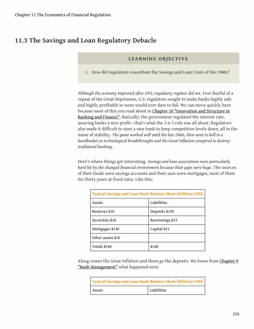
11.3 The Savings and Loan Regulatory Debacle
LEARNING OBJECTIVE
1. How did regulators exacerbate the Savings and Loan Crisis of the 1980s?
Although the economy improved after 1933, regulatory regimes did not. Ever fearful of arepeat of the Great Depression, U.S. regulators sought to make banks highly safeand highly profitable so none would ever dare to fail. We can move quickly herebecause most of this you read about in Chapter 10 "Innovation and Structure inBanking and Finance". Basically, the government regulated the interest rate,assuring banks a nice profit—that’s what the 3-6-3 rule was all about. Regulatorsalso made it difficult to start a new bank to keep competition levels down, all in thename of stability. The game worked well until the late 1960s, then went to hell in ahandbasket as technological breakthroughs and the Great Inflation conspired to destroytraditional banking.
Here’s where things get interesting. Savings and loan associations were particularlyhard hit by the changed financial environment because their gaps were huge. The sourcesof their funds were savings accounts and their uses were mortgages, most of themfor thirty years at fixed rates. Like this:
Typical Savings and Loan Bank Balance Sheet (Millions USD)
Assets Liabilities
Reserves $10 Deposits $130
Securities $10 Borrowings $15
Mortgages $130 Capital $15
Other assets $10
Totals $160 $160
Along comes the Great Inflation and there go the deposits. We know from Chapter 9"Bank Management" what happened next:
Typical Savings and Loan Bank Balance Sheet (Millions USD)
Assets Liabilities
Chapter 11 The Economics of Financial Regulation
235
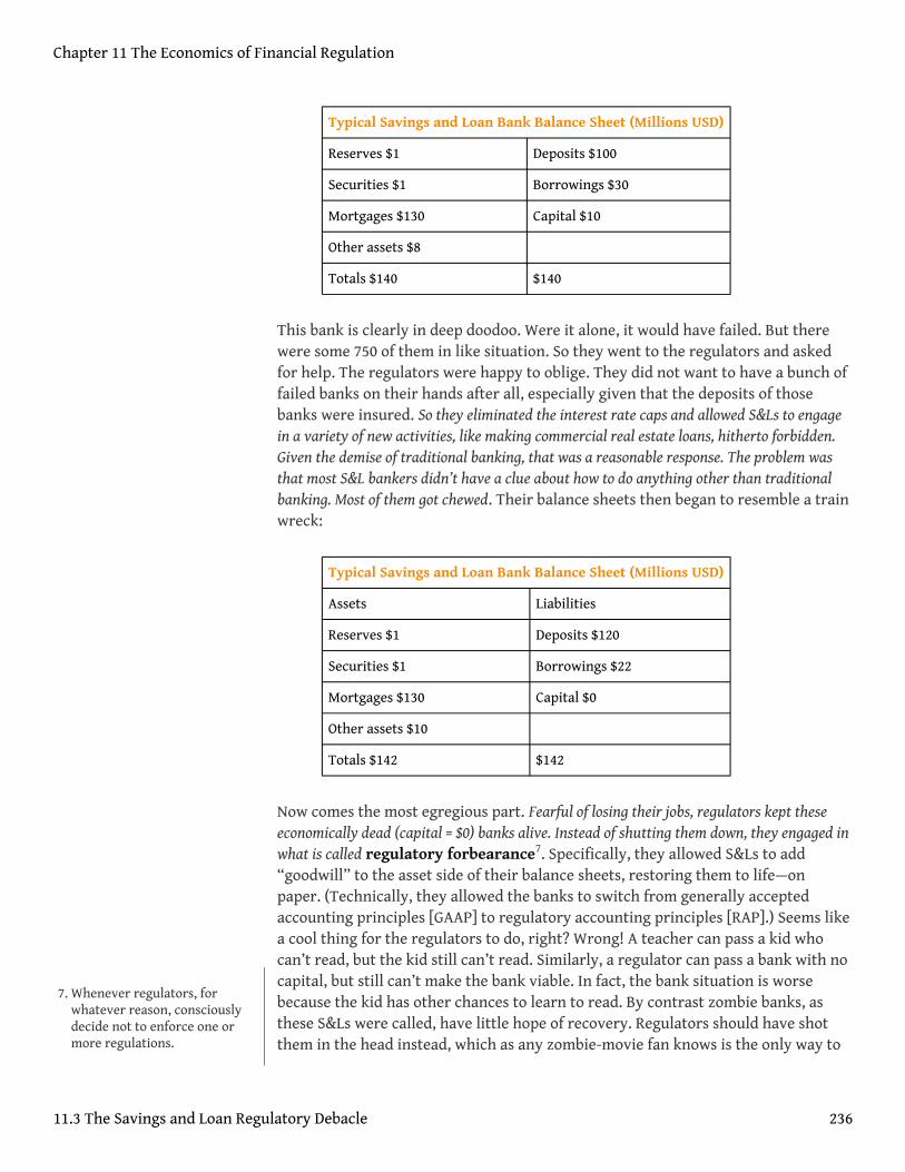
Typical Savings and Loan Bank Balance Sheet (Millions USD)
Reserves $1 Deposits $100
Securities $1 Borrowings $30
Mortgages $130 Capital $10
Other assets $8
Totals $140 $140
This bank is clearly in deep doodoo. Were it alone, it would have failed. But therewere some 750 of them in like situation. So they went to the regulators and askedfor help. The regulators were happy to oblige. They did not want to have a bunch offailed banks on their hands after all, especially given that the deposits of thosebanks were insured. So they eliminated the interest rate caps and allowed S&Ls to engagein a variety of new activities, like making commercial real estate loans, hitherto forbidden.Given the demise of traditional banking, that was a reasonable response. The problem wasthat most S&L bankers didn’t have a clue about how to do anything other than traditionalbanking. Most of them got chewed. Their balance sheets then began to resemble a trainwreck:
Typical Savings and Loan Bank Balance Sheet (Millions USD)
Assets Liabilities
Reserves $1 Deposits $120
Securities $1 Borrowings $22
Mortgages $130 Capital $0
Other assets $10
Totals $142 $142
Now comes the most egregious part. Fearful of losing their jobs, regulators kept theseeconomically dead (capital = $0) banks alive. Instead of shutting them down, they engaged inwhat is called regulatory forbearance7. Specifically, they allowed S&Ls to add“goodwill” to the asset side of their balance sheets, restoring them to life—onpaper. (Technically, they allowed the banks to switch from generally acceptedaccounting principles [GAAP] to regulatory accounting principles [RAP].) Seems likea cool thing for the regulators to do, right? Wrong! A teacher can pass a kid whocan’t read, but the kid still can’t read. Similarly, a regulator can pass a bank with nocapital, but still can’t make the bank viable. In fact, the bank situation is worsebecause the kid has other chances to learn to read. By contrast zombie banks, asthese S&Ls were called, have little hope of recovery. Regulators should have shotthem in the head instead, which as any zombie-movie fan knows is the only way to
7. Whenever regulators, forwhatever reason, consciouslydecide not to enforce one ormore regulations.
Chapter 11 The Economics of Financial Regulation
11.3 The Savings and Loan Regulatory Debacle 236

stop the undead dead in their tracks.http://www.margrabe.com/Devil/DevilU_Z.html;http://ericlathrop.com/notld/
Recall that if somebody has no capital, no skin in the game, to borrow WarrenBuffett’s phrase again, moral hazard will be extremely high because the person isplaying with other people’s money. In this case, the money wasn’t even that ofdepositors but rather of the deposit insurer, a government agency. The managers ofthe S&Ls did what anyone in the same situation would do: they rolled the dice, engaging inhighly risky investments funded with deposits and borrowings for which they paid a heftypremium. In other words, they borrowed from depositors and other lenders at highrates and invested in highly risky loans. A few got lucky and pulled their banks outof the red. Most of the risky loans, however, quickly turned sour. When the wholething was over, their balance sheets looked like this:
Typical Savings and Loan Bank Balance Sheet (Millions USD)
Assets Liabilities
Reserves $10 Deposits $200
Securities $10 Borrowings $100
Mortgages $100 Capital −$60
Goodwill $30
Crazy, risky loans $70
Other assets $20
Totals $240 $240
The regulators could no longer forbear. The insurance fund could not meet the depositliabilities of the thousands of failed S&Ls, so the bill ended up in the lap of U.S. taxpayers.
Chapter 11 The Economics of Financial Regulation
11.3 The Savings and Loan Regulatory Debacle 237
Stop and Think Box
In the 1980s, in response to the Great Inflation and the technologicalrevolution, regulators in Scandinavia (Sweden, Norway, and Finland)deregulated their heavily regulated banking systems. Bankers who usually lentonly to the best borrowers at government mandated rates suddenly foundthemselves competing for both depositors and borrowers. What happened?
Scandinavia suffered from worse banking crises than the United States. Inparticular, Scandinavian bankers were not very good at screening good frombad borrowers because they had long been accustomed to lending to just thebest. They inevitably made many mistakes, which led to defaults and ultimatelyasset and capital write-downs.
The most depressing aspect of this story is that the United States has unusuallygood regulators. As Figure 11.3 "Banking crises around the globe through 2002"shows, other countries have suffered through far worse banking crises andlosses. Note that at 3 percent of U.S. GDP, the S&L crisis was no picnic, but itpales in comparison to the losses in Argentina, Indonesia, China, Jamaica andelsewhere.
Chapter 11 The Economics of Financial Regulation
11.3 The Savings and Loan Regulatory Debacle 238
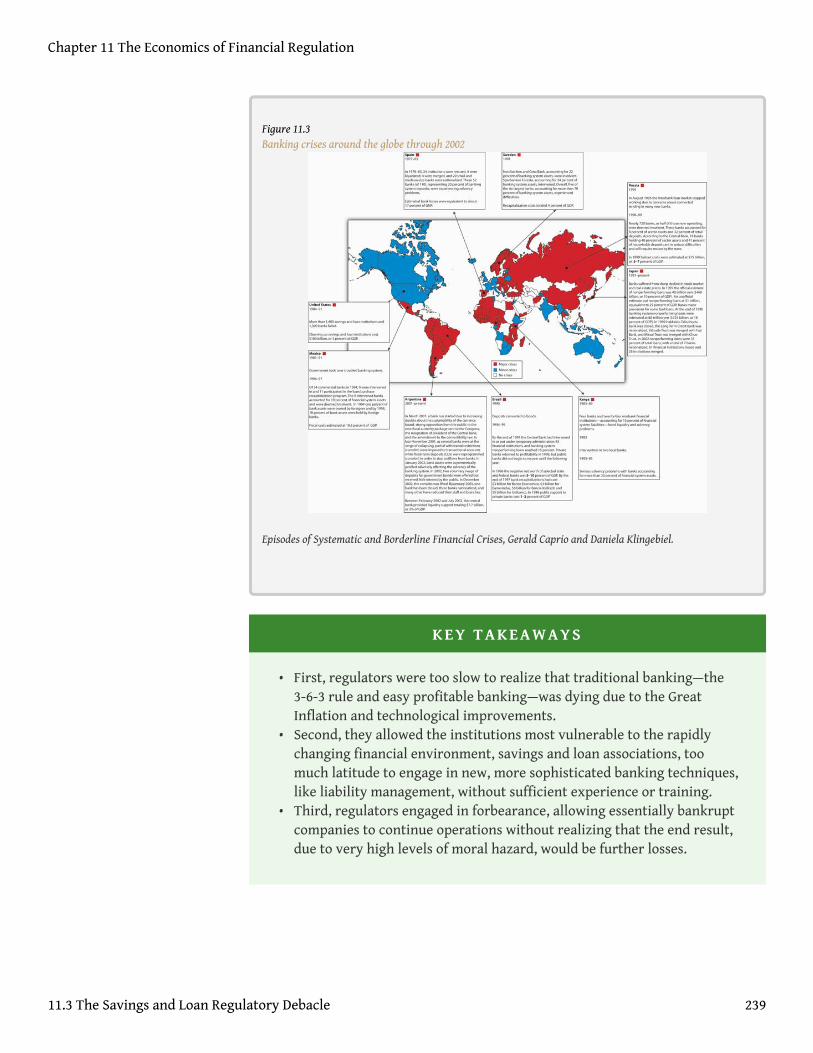
Figure 11.3Banking crises around the globe through 2002
Episodes of Systematic and Borderline Financial Crises, Gerald Caprio and Daniela Klingebiel.
KEY TAKEAWAYS
• First, regulators were too slow to realize that traditional banking—the3-6-3 rule and easy profitable banking—was dying due to the GreatInflation and technological improvements.
• Second, they allowed the institutions most vulnerable to the rapidlychanging financial environment, savings and loan associations, toomuch latitude to engage in new, more sophisticated banking techniques,like liability management, without sufficient experience or training.
• Third, regulators engaged in forbearance, allowing essentially bankruptcompanies to continue operations without realizing that the end result,due to very high levels of moral hazard, would be further losses.
Chapter 11 The Economics of Financial Regulation
11.3 The Savings and Loan Regulatory Debacle 239
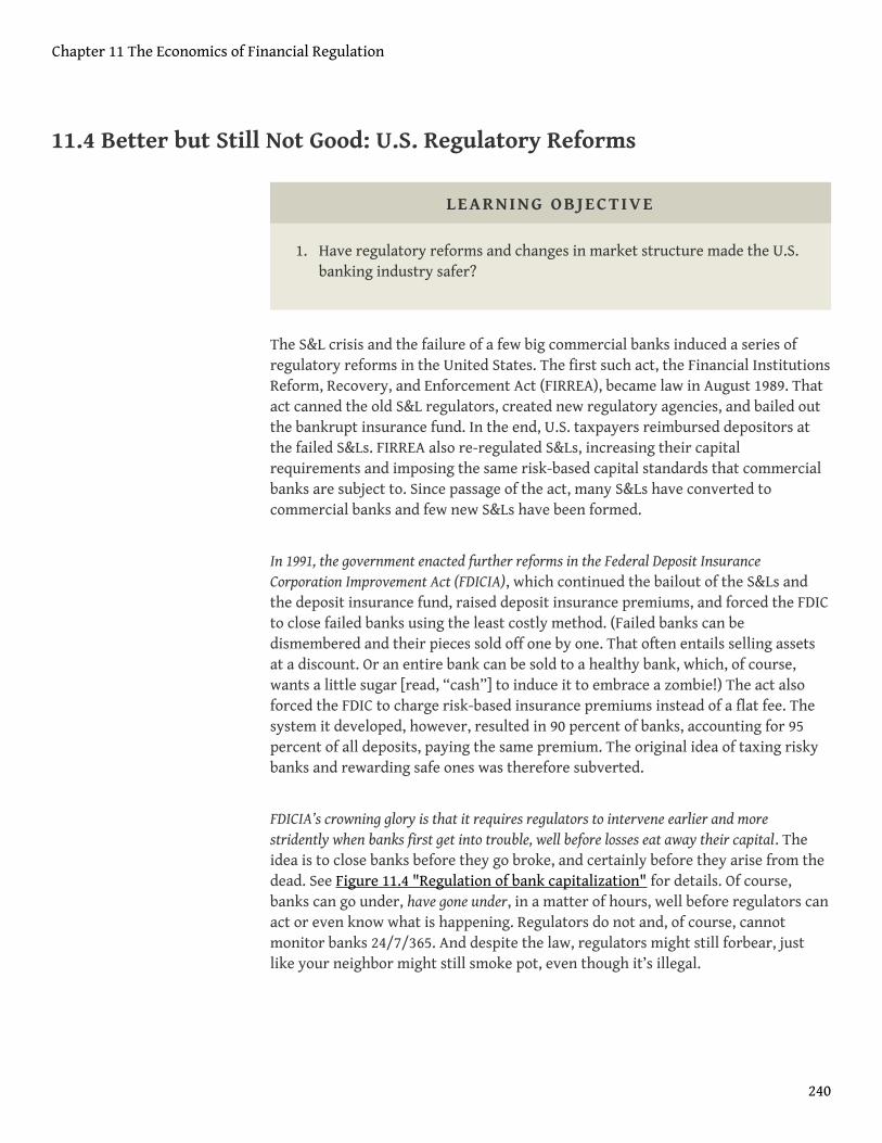
11.4 Better but Still Not Good: U.S. Regulatory Reforms
LEARNING OBJECTIVE
1. Have regulatory reforms and changes in market structure made the U.S.banking industry safer?
The S&L crisis and the failure of a few big commercial banks induced a series ofregulatory reforms in the United States. The first such act, the Financial InstitutionsReform, Recovery, and Enforcement Act (FIRREA), became law in August 1989. Thatact canned the old S&L regulators, created new regulatory agencies, and bailed outthe bankrupt insurance fund. In the end, U.S. taxpayers reimbursed depositors atthe failed S&Ls. FIRREA also re-regulated S&Ls, increasing their capitalrequirements and imposing the same risk-based capital standards that commercialbanks are subject to. Since passage of the act, many S&Ls have converted tocommercial banks and few new S&Ls have been formed.
In 1991, the government enacted further reforms in the Federal Deposit InsuranceCorporation Improvement Act (FDICIA), which continued the bailout of the S&Ls andthe deposit insurance fund, raised deposit insurance premiums, and forced the FDICto close failed banks using the least costly method. (Failed banks can bedismembered and their pieces sold off one by one. That often entails selling assetsat a discount. Or an entire bank can be sold to a healthy bank, which, of course,wants a little sugar [read, “cash”] to induce it to embrace a zombie!) The act alsoforced the FDIC to charge risk-based insurance premiums instead of a flat fee. Thesystem it developed, however, resulted in 90 percent of banks, accounting for 95percent of all deposits, paying the same premium. The original idea of taxing riskybanks and rewarding safe ones was therefore subverted.
FDICIA’s crowning glory is that it requires regulators to intervene earlier and morestridently when banks first get into trouble, well before losses eat away their capital. Theidea is to close banks before they go broke, and certainly before they arise from thedead. See Figure 11.4 "Regulation of bank capitalization" for details. Of course,banks can go under, have gone under, in a matter of hours, well before regulators canact or even know what is happening. Regulators do not and, of course, cannotmonitor banks 24/7/365. And despite the law, regulators might still forbear, justlike your neighbor might still smoke pot, even though it’s illegal.
Chapter 11 The Economics of Financial Regulation
240
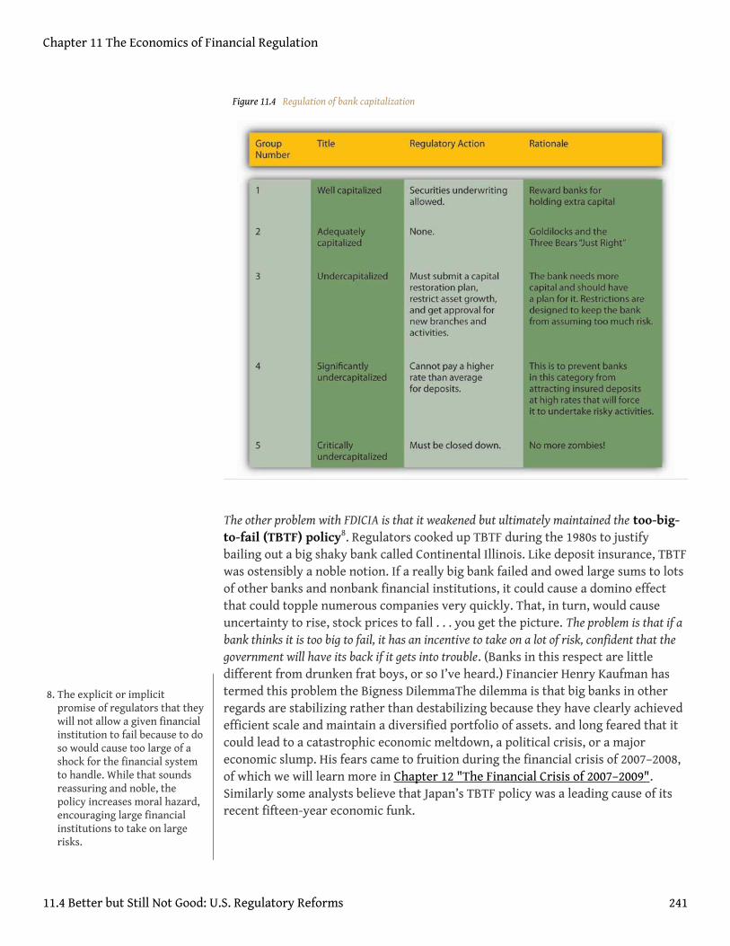
Figure 11.4 Regulation of bank capitalization
The other problem with FDICIA is that it weakened but ultimately maintained the too-big-to-fail (TBTF) policy8. Regulators cooked up TBTF during the 1980s to justifybailing out a big shaky bank called Continental Illinois. Like deposit insurance, TBTFwas ostensibly a noble notion. If a really big bank failed and owed large sums to lotsof other banks and nonbank financial institutions, it could cause a domino effectthat could topple numerous companies very quickly. That, in turn, would causeuncertainty to rise, stock prices to fall . . . you get the picture. The problem is that if abank thinks it is too big to fail, it has an incentive to take on a lot of risk, confident that thegovernment will have its back if it gets into trouble. (Banks in this respect are littledifferent from drunken frat boys, or so I’ve heard.) Financier Henry Kaufman hastermed this problem the Bigness DilemmaThe dilemma is that big banks in otherregards are stabilizing rather than destabilizing because they have clearly achievedefficient scale and maintain a diversified portfolio of assets. and long feared that itcould lead to a catastrophic economic meltdown, a political crisis, or a majoreconomic slump. His fears came to fruition during the financial crisis of 2007–2008,of which we will learn more in Chapter 12 "The Financial Crisis of 2007–2009".Similarly some analysts believe that Japan’s TBTF policy was a leading cause of itsrecent fifteen-year economic funk.
8. The explicit or implicitpromise of regulators that theywill not allow a given financialinstitution to fail because to doso would cause too large of ashock for the financial systemto handle. While that soundsreassuring and noble, thepolicy increases moral hazard,encouraging large financialinstitutions to take on largerisks.
Chapter 11 The Economics of Financial Regulation
11.4 Better but Still Not Good: U.S. Regulatory Reforms 241
In 1994, the Riegle-Neal Interstate Banking and Branching Efficiency Act finallyoverturned most prohibitions on interstate banking. As discussed in Chapter 10"Innovation and Structure in Banking and Finance", that law led to considerableconsolidation, the effects of which are still unclear. Nevertheless, the act was longoverdue, as was the Gramm-Leach-Bliley Financial Services Modernization Act of1999, which repealed Glass-Steagall, allowing the same institutions to engage inboth commercial and investment banking activities. The act has led to someconglomeration, but not as much as many observers expected. Again, it may besome time before the overall effects of the reform become clear. So far, both actsappear to have strengthened the financial system by making banks more profitableand diversified. So far, some large complex banking organizations and largecomplex financial institutions (LCBOs and LCFIs, respectively) have held up well inthe face of the subprime mortgage crisis, but others have failed. The crisis appearsrooted in more fundamental issues, like TBTF and a dearth of internal incentivealignment within financial institutions, big and small.
KEY TAKEAWAYS
• To some extent, it is too early to tell what the effects of financialconsolidation, concentration, and conglomeration will be.
• Overall, it appears that recent U.S. financial reforms range from salutary(repeal of branching restrictions and Glass-Steagall) to destabilizing(retention of the too-big-to-fail policy).
Chapter 11 The Economics of Financial Regulation
11.4 Better but Still Not Good: U.S. Regulatory Reforms 242
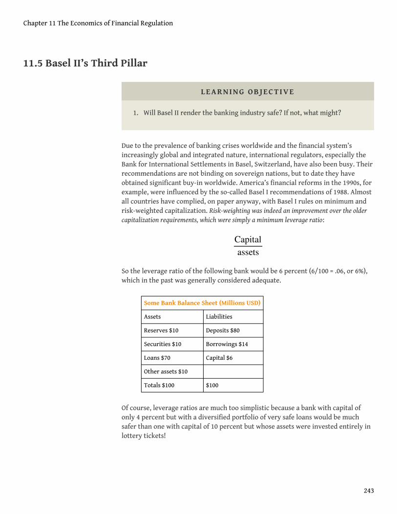
11.5 Basel II’s Third Pillar
LEARNING OBJECTIVE
1. Will Basel II render the banking industry safe? If not, what might?
Due to the prevalence of banking crises worldwide and the financial system’sincreasingly global and integrated nature, international regulators, especially theBank for International Settlements in Basel, Switzerland, have also been busy. Theirrecommendations are not binding on sovereign nations, but to date they haveobtained significant buy-in worldwide. America’s financial reforms in the 1990s, forexample, were influenced by the so-called Basel I recommendations of 1988. Almostall countries have complied, on paper anyway, with Basel I rules on minimum andrisk-weighted capitalization. Risk-weighting was indeed an improvement over the oldercapitalization requirements, which were simply a minimum leverage ratio:
So the leverage ratio of the following bank would be 6 percent (6/100 = .06, or 6%),which in the past was generally considered adequate.
Some Bank Balance Sheet (Millions USD)
Assets Liabilities
Reserves $10 Deposits $80
Securities $10 Borrowings $14
Loans $70 Capital $6
Other assets $10
Totals $100 $100
Of course, leverage ratios are much too simplistic because a bank with capital ofonly 4 percent but with a diversified portfolio of very safe loans would be muchsafer than one with capital of 10 percent but whose assets were invested entirely inlottery tickets!
Capitalassets
Chapter 11 The Economics of Financial Regulation
243
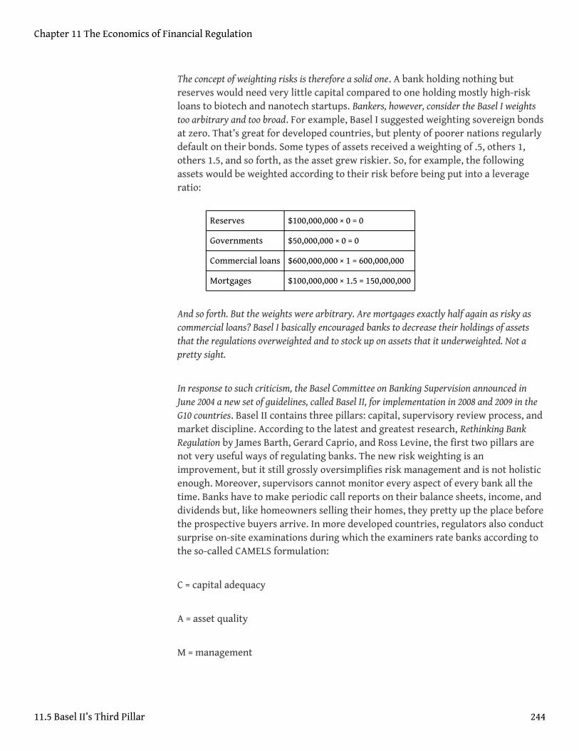
The concept of weighting risks is therefore a solid one. A bank holding nothing butreserves would need very little capital compared to one holding mostly high-riskloans to biotech and nanotech startups. Bankers, however, consider the Basel I weightstoo arbitrary and too broad. For example, Basel I suggested weighting sovereign bondsat zero. That’s great for developed countries, but plenty of poorer nations regularlydefault on their bonds. Some types of assets received a weighting of .5, others 1,others 1.5, and so forth, as the asset grew riskier. So, for example, the followingassets would be weighted according to their risk before being put into a leverageratio:
Reserves $100,000,000 × 0 = 0
Governments $50,000,000 × 0 = 0
Commercial loans $600,000,000 × 1 = 600,000,000
Mortgages $100,000,000 × 1.5 = 150,000,000
And so forth. But the weights were arbitrary. Are mortgages exactly half again as risky ascommercial loans? Basel I basically encouraged banks to decrease their holdings of assetsthat the regulations overweighted and to stock up on assets that it underweighted. Not apretty sight.
In response to such criticism, the Basel Committee on Banking Supervision announced inJune 2004 a new set of guidelines, called Basel II, for implementation in 2008 and 2009 in theG10 countries. Basel II contains three pillars: capital, supervisory review process, andmarket discipline. According to the latest and greatest research, Rethinking BankRegulation by James Barth, Gerard Caprio, and Ross Levine, the first two pillars arenot very useful ways of regulating banks. The new risk weighting is animprovement, but it still grossly oversimplifies risk management and is not holisticenough. Moreover, supervisors cannot monitor every aspect of every bank all thetime. Banks have to make periodic call reports on their balance sheets, income, anddividends but, like homeowners selling their homes, they pretty up the place beforethe prospective buyers arrive. In more developed countries, regulators also conductsurprise on-site examinations during which the examiners rate banks according tothe so-called CAMELS formulation:
C = capital adequacy
A = asset quality
M = management
Chapter 11 The Economics of Financial Regulation
11.5 Basel II’s Third Pillar 244
E = earnings
L = liquidity (reserves)
S = sensitivity to market risk.
A, M, and S are even more difficult to ascertain than C, E, and L and, as noted above,any or all of the variables can change very rapidly. Moreover, as discussed inChapter 10 "Innovation and Structure in Banking and Finance", much bankingactivity these days takes place off the balance sheet, where it is even more difficult forregulators to find and accurately assess. Finally, in many jurisdictions, examiners arenot paid well and hence do not do a very thorough job.
Barth, Caprio, and Levine argue that the third pillar of Basel II, financial marketmonitoring, is different. In aggregate, market participants can and in fact domonitor banks and bankers much more often and much more astutely thanregulators can because they have much more at stake than a relatively low-payingjob. Barth, Caprio, and Levine argue persuasively that instead of conceiving of themselves aspolice officers, judges, and juries, bank regulators should see themselves as aides, as helpingbank depositors (and other creditors of the bank) and stockholders to keep the bankers inline. After all, nobody gains from a bank’s failure. The key, they believe, is to ensurethat debt and equity holders have incentives and opportunities to monitor bankmanagement to ensure that they are not taking on too much risk. That meansreducing asymmetric information by ensuring reliable information disclosure andurging that corporate governance best practices be followed.Frederick D. Lipman,Corporate Governance Best Practices: Strategies for Public, Private, and Not-for-ProfitOrganizations (Hoboken, N.J.: Wiley, 2006).
Regulators can also provide banks with incentives to keep their asset bases sufficientlydiversified and to prevent them from engaging in inappropriate activities, like buildingrocket ships or running water treatment plants. Screening new banks and bankers, ifregulators do it to reduce adverse selection (omit shysters or inexperienced people)rather than to aid existing banks (by blocking all or most new entrants and hencelimiting competition) or to line their own pockets (via bribes), is another areawhere regulators can be effective. By focusing on a few key reachable goals,regulators can concentrate their limited resources and get the job done, the job ofletting people look after their own property themselves. The market-basedapproach, scholars note, is most important in less-developed countries whereregulators are more likely to be on the take (to enact and enforce regulationssimply to augment their incomes via bribes).
Chapter 11 The Economics of Financial Regulation
11.5 Basel II’s Third Pillar 245
In July 2010, in the wake of the worst financial dislocation in 80 years, the U.S.government attempted to make the financial system less fragile by passing theDodd-Frank Wall Street Reform and Protection Act. Over the next several years, thelaw mandates the creation of a new:
• Financial Stability Oversight Council;• Office of Financial Research;• Consumer Financial Protection Bureau;• advanced warning system that will attempt to identify and address
systemic risks before they threaten financial institutions and markets.
It also calls for:
• more stringent capital and liquidity requirements for LCFIs;• tougher regulation of systemically important non-bank financial
companies;• the breakup of LCFIs, if necessary;• tougher restrictions on bailouts;• more transparency for asset-backed securities and other “exotic”
financial instruments;• improved corporate governance rules designed to give shareholders
more say over the structure of executive compensation.
Despite the sweeping nature of those reforms, some scholars remain skeptical ofthe new law because it has not clearly eliminated the problems associated withTBTF policy, bailouts, and other causes of the financial crisis of 2007-2009.
Chapter 11 The Economics of Financial Regulation
11.5 Basel II’s Third Pillar 246
KEY TAKEAWAYS
• Basel I and II have provided regulators with more sophisticated ways ofanalyzing the adequacy of bank capital.
• Nevertheless, it appears that regulators lag behind banks and theirbankers, in part because of agency problems within regulatorybureaucracies and in part because of the gulf of asymmetric informationseparating banks and regulators, particularly when it comes to thequality of assets and the extent and risk of off-balance-sheet activities.
• If scholars like Barth, Caprio, and Levine are correct, regulators ought tothink of ways of helping financial markets, particularly bank debt andequity holders, to monitor banks.
• They should also improve their screening of new bank applicantswithout unduly restricting entry, and set and enforce broad guidelinesfor portfolio diversification and admissible activities.
Chapter 11 The Economics of Financial Regulation
11.5 Basel II’s Third Pillar 247
11.6 Suggested Reading
Acharya, Viral et al, eds. Regulating Wall Street: The Dodd-Frank Act and the NewArchitecture of Global Finance. Hoboken, NJ: John Wiley and Sons, 2011.
Arner, Douglas. Financial Stability, Economic Growth, and the Role of Law. New York:Cambridge University Press, 2007.
Barth, James, Gerard Caprio, and Ross Levine. Rethinking Bank Regulation. New York:Cambridge University Press, 2006.
Barth, James, S. Trimbath, and Glenn Yago. The Savings and Loan Crisis: Lessons from aRegulatory Failure. New York: Springer, 2004.
Benston, George. Regulating Financial Markets: A Critique and Some Proposals.Washington, DC: AEI Press, 1999.
Bernanke, Ben S. Essays on the Great Depression. Princeton, NJ: Princeton UniversityPress, 2000.
Gup, Benton. Too Big to Fail: Policies and Practices in Government Bailouts. Westport, CT:Praeger, 2004.
Stern, Gary, and Ron Feldman. Too Big to Fail: The Hazards of Bank Bailouts.Washington, DC: Brookings Institution Press, 2004.
Tullick, Gordon, Arthur Seldon, and Gordon Brady. Government Failure: A Primer inPublic Choice. Washington, DC: Cato Institute, 2002.
Winston, Clifford. Government Failure Versus Market Failure: Microeconomics PolicyResearch and Government Performance. Washington, DC: AEI-Brookings Joint Centerfor Regulatory Studies, 2006.
Chapter 11 The Economics of Financial Regulation
248
Chapter 12
The Financial Crisis of 2007–2009
CHAPTER OBJECTIVES
By the end of this chapter, students should be able to:
1. Define financial crisis and differentiate between systemic andnonsystemic crises.
2. Describe a generic asset bubble.3. Define leverage and explain its role in asset bubble formation.4. Explain why bubbles burst, causing financial panics.5. Define and explain the importance of lender of last resort.6. Define and explain the importance of bailouts.7. Narrate the causes and consequences of the financial crisis that began in
2007.
249
12.1 Financial Crises
LEARNING OBJECTIVE
1. What is a financial crisis?
A financial crisis1occurs when one or more financial markets or intermediaries ceasefunctioning or function only erratically and inefficiently. A nonsystemic crisis2 involvesonly one or a few markets or sectors, like the Savings and Loan Crisis described inChapter 11 "The Economics of Financial Regulation". A systemic crisis3 involves all,or almost all, of the financial system to some extent, as during the GreatDepression.
Financial crises are neither new nor unusual. Thousands of crises, including theinfamous Tulip Mania and South Sea Company episodes, have rocked financialsystems throughout the world in the past five hundred years. Two such crises, in1764–1768 and 1773, helped lead to the American Revolution.Tim Arango, “TheHousing-Bubble and the American Revolution,” New York Times (29 November 2008),WK5. http://www.nytimes.com/2008/11/30/weekinreview/30arango.html?_r=2&pagewanted=1&ref=weekinreview After its independence, theUnited States suffered systemic crises in 1792, 1818–1819, 1837–1839, 1857, 1873,1884, 1893–1895, 1907, 1929–1933, and 2008. Nonsystemic crises have been evenmore numerous and include the credit crunch of 1966, stock market crashes in1973–1974 (when the Dow dropped from a 1,039 close on January 12, 1973, to a 788close on December 5, 1973, to a 578 close on December 6, 1974) and 1987, the failureof Long-Term Capital Management in 1998, the dot-com troubles of 2000, thedramatic events following the terrorist attacks in 2001, and the subprime mortgagedebacle of 2007. Sometimes, nonsystemic crises burn out or are brought undercontrol before they spread to other parts of the financial system. Other times, as in1929 and 2007, nonsystemic crises spread like a wildfire until they threaten to burnthe entire system.
1. The functioning of one or morefinancial markets orintermediaries becomes erraticor ceases altogether.
2. A particular market orintermediary functionserratically or inefficiently.
3. The functioning of all, ornearly all, of the financialsystem degrades.
Chapter 12 The Financial Crisis of 2007–2009
250
Stop and Think Box
“While we ridicule ancient superstition we have an implicit faith in the bubblesof banking, and yet it is difficult to discover a greater absurdity, in ascribingomnipotence to bulls, cats and onions, than for a man to carry about a thousandacres of land . . . in his pocket book. . . . This gross bubble is practiced every day,even upon the infidelity of avarice itself. . . . So we see wise and honestAmericans, of the nineteenth century, embracing phantoms for realities, andrunning mad in schemes of refinement, tastes, pleasures, wealth and power, bythe soul [sic] aid of this hocus pocus.”—Cause of, and Cure for, HardTimes.http://books.google.com/books When were these words penned? How doyou know?
This was undoubtedly penned during one of the nineteenth century U.S.financial crises mentioned above. Note the negative tone, the allusion toAmericans, and the reference to the nineteenth century. In fact, the pamphletappeared in 1818. For a kick, compare/contrast it to blogs bemoaning the crisisthat began in 2007:
http://cartledged.blogspot.com/2007/09/greedy-bastards-club.html
http://www.washingtonmonthly.com/archives/individual/2008_03/013339.php
http://thedefenestrators.blogspot.com/2008/10/death-to-bankers.html
Both systemic and nonsystemic crises damage the real economy by preventing the normalflow of credit from savers to entrepreneurs and other businesses and by making it moredifficult or expensive to spread risks. Given the damage financial crises can cause,scholars and policymakers are keenly interested in their causes and consequences.You should be, too.
Chapter 12 The Financial Crisis of 2007–2009
12.1 Financial Crises 251
KEY TAKEAWAYS
• Throughout history, systemic (widespread) and nonsystemic (confinedto a few industries) financial crises have damaged the real economy bydisrupting the normal flow of credit and insurance.
• Understanding the causes and consequences of financial crises istherefore important.
Chapter 12 The Financial Crisis of 2007–2009
12.1 Financial Crises 252
12.2 Asset Bubbles
LEARNING OBJECTIVE
1. What are asset bubbles and what role does leverage play in theircreation?
Asset bubbles4are rapid increases in the value of some asset, like bonds, commodities(cotton, gold, oil, tulips), equities, or real estate. Some combination of low interest rates,new technology, unprecedented increases in demand for the asset, and leveragetypically create bubbles.
Low interest rates can cause bubbles by lowering the total cost of asset ownership. Recallfrom Chapter 4 "Interest Rates" that interest rates and bond prices are inverselyrelated. Algebraically, the i term is in the denominator of the PV formula—PV =FV/(1 + i)n—so as it gets smaller, PV must get larger (holding FV constant, ofcourse).
4. In this context, a rapid increasein asset prices that is not easilyjustified by fundamentals likeexpected earnings, interestrates, and the like.
Chapter 12 The Financial Crisis of 2007–2009
253
Stop and Think Box
In colonial New York in the 1740s and 1750s, interest rates on mortgages weregenerally 8 percent. In the late 1750s and early 1760s, they fell to about 4percent, and expected revenues from land ownership increased by about 50percent. What happened to real estate prices? Why?
They rose significantly because it was cheaper to borrow money, thus loweringthe total cost of real estate ownership, and because the land was expected tocreate higher revenues. Thinking of the land as a perpetuity and FV as theexpected revenues arising from it:
And that is just the real estate effect. Increasing FV by £50 leads to thefollowing:
In 1762, Benjamin Franklin reported that the “Rent of old Houses, and Value ofLands, . . . are trebled in the last Six Years.”For more on the crisis, see TimArango, “The Housing-Bubble Revolution,” New York Times (30 November 2008),WK 5. http://www.nytimes.com/2008/11/30/weekinreview/30arango.html?_r=2&pagewanted=1&ref=weekinreview
The effect of new technology can be thought of as increasing FV, leading, of course, to ahigher PV. Or, in the case of equities, low interest rates decrease k (required return)and new inventions increase g (constant growth rate) in the Gordon growthmodel—P = E × (1 + g)/(k – g)—both of which lead to a higher price.
Large increases in the demand for an asset occur for a variety of reasons. Demandcan be increased merely by investors’ expectations of higher prices in the future, as in theone period valuation model—P = E/(1 + k) + P1/(1 + k). If many investors believe that P1
must be greater than P a year (or any other period) hence, demand for the asset willincrease and the expectation of a higher P1 will be vindicated. That sometimes leads
PV = FV/i
PV = £100/.08 = £1,250
PV = £100/.04 = £2,500
PV = £150/.04 = £3,750, or a tripling of prices.
Chapter 12 The Financial Crisis of 2007–2009
12.2 Asset Bubbles 254
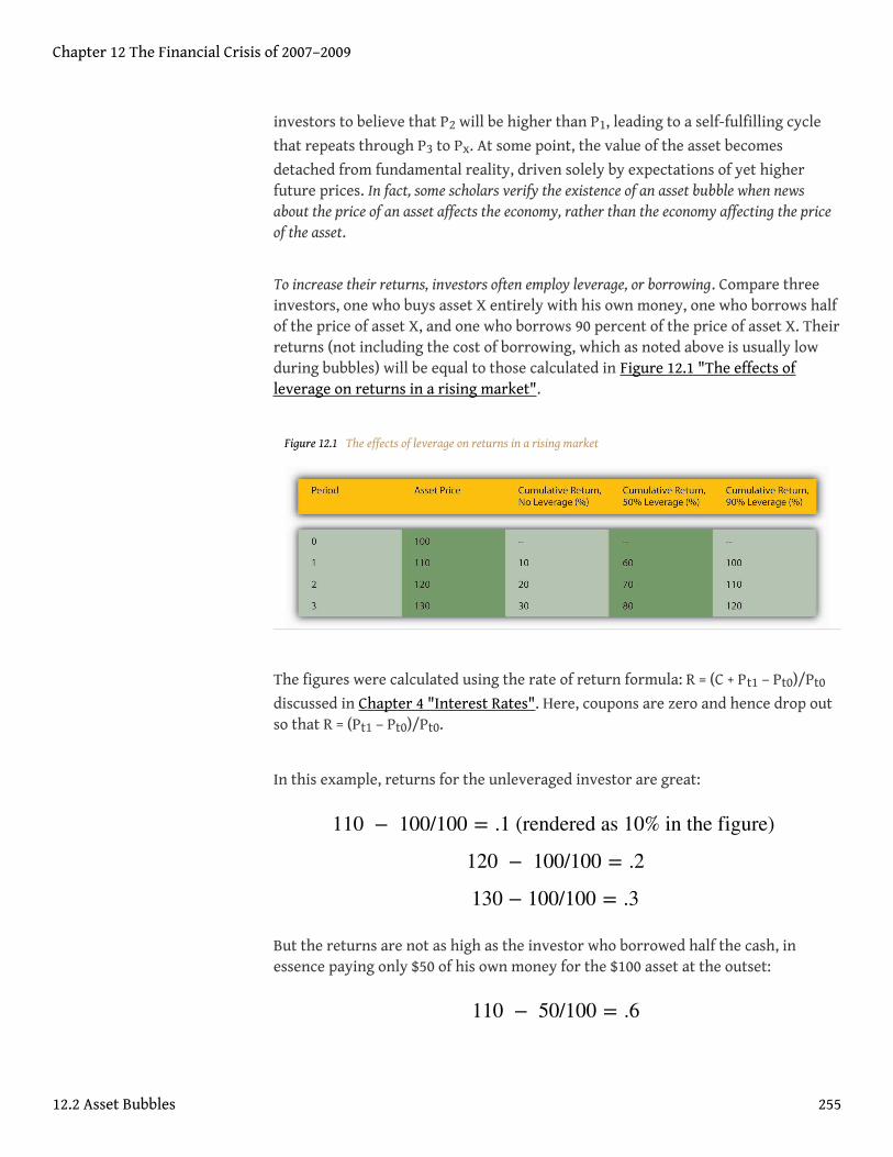
investors to believe that P2 will be higher than P1, leading to a self-fulfilling cycle
that repeats through P3 to Px. At some point, the value of the asset becomes
detached from fundamental reality, driven solely by expectations of yet higherfuture prices. In fact, some scholars verify the existence of an asset bubble when newsabout the price of an asset affects the economy, rather than the economy affecting the priceof the asset.
To increase their returns, investors often employ leverage, or borrowing. Compare threeinvestors, one who buys asset X entirely with his own money, one who borrows halfof the price of asset X, and one who borrows 90 percent of the price of asset X. Theirreturns (not including the cost of borrowing, which as noted above is usually lowduring bubbles) will be equal to those calculated in Figure 12.1 "The effects ofleverage on returns in a rising market".
Figure 12.1 The effects of leverage on returns in a rising market
The figures were calculated using the rate of return formula: R = (C + Pt1 – Pt0)/Pt0
discussed in Chapter 4 "Interest Rates". Here, coupons are zero and hence drop outso that R = (Pt1 – Pt0)/Pt0.
In this example, returns for the unleveraged investor are great:
But the returns are not as high as the investor who borrowed half the cash, inessence paying only $50 of his own money for the $100 asset at the outset:
110 − 100/100 = .1 (rendered as 10% in the figure)
120 − 100/100 = .2
130 − 100/100 = .3
110 − 50/100 = .6
Chapter 12 The Financial Crisis of 2007–2009
12.2 Asset Bubbles 255
But even he looks like a chump compared to the investor who borrowed most of themoney to finance the original purchase, putting up only $10 of his own money:
If you are thinking the most highly leveraged investor is the smart one, go back and rereadthe section of Chapter 2 "The Financial System"that discusses the trade-off between riskand return before continuing.
KEY TAKEAWAYS
• Asset bubbles occur when the prices of some asset, like stocks or realestate, increase rapidly due to some combination of low interest rates,high leverage, new technology, and large, often self-fulfilling shifts indemand.
• The expectation of higher prices in the future, combined with highlevels of borrowing, allow asset prices to detach from their underlyingeconomic fundamentals.
120 − 50/100 = .7
130 − 50/100 = .8
110 − 10/100 = 1
120 − 10 = 1.1
130 − 10 = 1.2
Chapter 12 The Financial Crisis of 2007–2009
12.2 Asset Bubbles 256
12.3 Financial Panics
LEARNING OBJECTIVE
1. What are financial panics and what causes them?
A financial panic5occurs when leveraged financial intermediaries and other investorsmust sell assets quickly in order to meet lenders’ calls6. Lenders call loans, or ask forrepayment, when interest rates increase and/or when the value of collateralpledged to repay the loan sinks below the amount the borrower owes. Calls are anormal part of everyday business, but during a panic, they all come en masse due tosome shock, often the bursting7 of an asset bubble. Bubbles, like people, are boundto die but nobody knows in advance when they will do so. A burst is sometimestriggered by an obvious shock, like a natural catastrophe or the failure of animportant company, but sometimes something as seemingly innocuous as a largesell order can touch them off.
During a panic, almost everybody must sell and few can or want to buy, so pricesplummet, triggering additional calls, and yet more selling. Invariably, someinvestors, usually the most highly leveraged ones, cannot sell assets quicklyenough, or for a high enough price, to “meet the call” and repay their loans. Banksand other lenders begin to suffer defaults. Their lenders (other banks, depositors,holders of commercial paper), in turn, begin to wonder if they are still credit-worthy. Asymmetric information and uncertainty, as described in Chapter 11 "TheEconomics of Financial Regulation", reign supreme, inducing lenders to restrictcredit. At some point, investors’ emotions take over, and they literally go into a panic, onethat makes Tony Soprano’s panic attacks seem like a stroll in thepark.http://www.menshealth.com/cda/article.do?site=MensHealth&channel=health&category=stress.management&conitem=04f999edbbbd201099edbbbd2010cfe793cd____
Panics often cause the rapid de-leveraging8of the financial system, a period when interestrates for riskier types of loans and securities increase and/or when a credit crunch9, or alarge decrease in the volume of lending, takes place. Such conditions often usher in anegative bubble10, a period when high interest rates, tight credit, and expectationsof lower asset prices in the future cause asset values to trend downward, sometimeswell below the values indicated by underlying economic fundamentals. During de-leveraging, the forces that drove asset prices up now conspire to drag them lower.
5. Panicked selling occurs duringthe rapid de-leveraging of thefinancial system following thebursting of an asset bubble.
6. A lender asks a borrower torepay, usually because interestrates have increased and/orthe value of collateral hasdeclined.
7. When an asset bubble rapidlydeflates, i.e., the price of theasset rapidly decreases.
8. Lenders force borrowers toinvest more of their own equityin assets.
9. The volume of loans decreasesdramatically, usually inresponse to the bursting of anasset bubble during a financialcrisis.
10. A bubble characterized byprices that are far below theirrational value.
Chapter 12 The Financial Crisis of 2007–2009
257
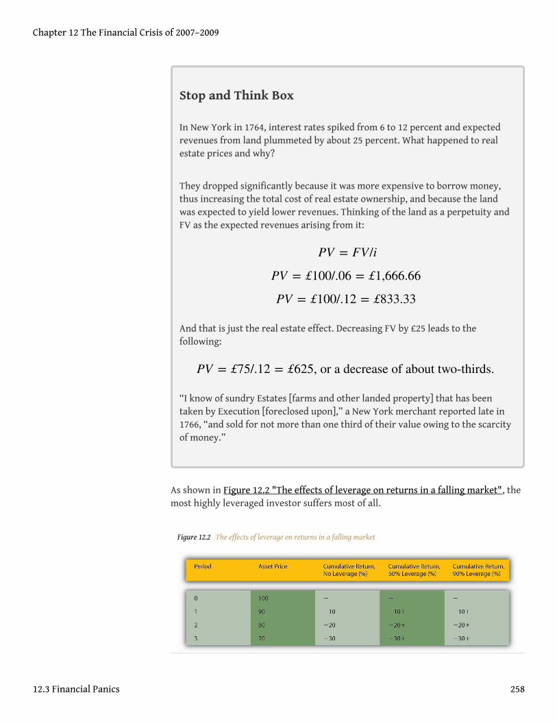
Stop and Think Box
In New York in 1764, interest rates spiked from 6 to 12 percent and expectedrevenues from land plummeted by about 25 percent. What happened to realestate prices and why?
They dropped significantly because it was more expensive to borrow money,thus increasing the total cost of real estate ownership, and because the landwas expected to yield lower revenues. Thinking of the land as a perpetuity andFV as the expected revenues arising from it:
And that is just the real estate effect. Decreasing FV by £25 leads to thefollowing:
“I know of sundry Estates [farms and other landed property] that has beentaken by Execution [foreclosed upon],” a New York merchant reported late in1766, “and sold for not more than one third of their value owing to the scarcityof money.”
As shown in Figure 12.2 "The effects of leverage on returns in a falling market", themost highly leveraged investor suffers most of all.
Figure 12.2 The effects of leverage on returns in a falling market
PV = FV/i
PV = £100/.06 = £1,666.66
PV = £100/.12 = £833.33
PV = £75/.12 = £625, or a decrease of about two-thirds.
Chapter 12 The Financial Crisis of 2007–2009
12.3 Financial Panics 258
Again, I used the rate of return formula, but coupons are zero so that R = (Pt1 –
Pt0)/Pt0. As the price of the asset falls, the unleveraged investor suffers negative
returns:
The leveraged investors lose the same percentage and must now pay a high interestrate for their loans, or put up the equity themselves, at a time when theopportunity cost of doing so is substantial:
The higher the leverage, the larger the sum that must be borrowed at high rates.
Also, the higher the leverage, the smaller the price change needs to be to trigger acall. At 50 percent leverage, a $100 asset could drop to $50 before the lender mustcall. At 90 percent leverage, a $100 asset need lose only $10 to induce a call.
KEY TAKEAWAYS
• The bursting of an asset bubble, or the rapidly declining prices of anasset class, usually leads to a financial panic, reductions in the quantityof available credit, and the de-leveraging of the financial system.
• The most highly leveraged investors suffer most.
90 − 100/100 = −.1
80 − 100/100 = −.2
70 − 100/100 = −.3
(90 − 50 + 50)/100 = − .1 + interest on $50
(80 - 50 + 50)/100 = -.2 + interest on $50
(70 − 50 + 50)/100 = − .3 + interest on $50
(90 − 90 + 90)/100 = −.1 + interest on $90
(80 − 90 + 90)/100 = −.2 + interest on $90
(70 − 90 + 90)/100 = −.3 + interest on $90
Chapter 12 The Financial Crisis of 2007–2009
12.3 Financial Panics 259
12.4 Lender of Last Resort
LEARNING OBJECTIVE
1. What is a lender of last resort and what does it do?
As noted above, financial panics and the de-leveraging that often occur after themcan wreak havoc on the real economy by decreasing the volume of loans, insurancecontracts, and other beneficial financial products. That, in turn, can cause firms toreduce output and employment. Lenders of last resort try to stop panics and de-leveraging by adding liquidity to the financial system and/or attempting to restore investorconfidence. They add liquidity by increasing the money supply, reducing interestrates, and making loans to worthy borrowers who find themselves shut off fromtheir normal sources of external finance. They try to restore investor confidence bymaking upbeat statements about the overall health of the economy and/or financialsystem and by implementing policies that investors are likely to find beneficial.During the darkest days of 1933, for example, the U.S. federal government restoredconfidence in the banking system through strong executive leadership and bycreating the Federal Deposit Insurance Corporation.
Chapter 12 The Financial Crisis of 2007–2009
260
Stop and Think Box
In a single day, October 19, 1987, the S&P fell by 20 percent. What caused such arapid decline? Why did the panic not result in de-leveraging or recession?
According to a short history of the event by Mark Carlson (“A Brief History ofthe 1987 Stock Market Crash with a Discussion of the Federal ReserveResponse”),http://www.federalreserve.gov/Pubs/feds/2007/200713/200713pap.pdf “During the years prior to the crash, equity markets had beenposting strong gains. . . . There had been an influx of new investors. . . . Equitieswere also boosted by some favorable tax treatments given to the financing ofcorporate buyouts. . . . The macroeconomic outlook during the months leadingup to the crash had become somewhat less certain. . . . Interest rates wererising globally. . . . A growing U.S. trade deficit and decline in the value of thedollar were leading to concerns about inflation and the need for higher interestrates in the U.S. as well.” On the day of the crash, investors learned that deficitswere higher than expected and that the favorable tax rules might change. Asprices dropped, “record margin calls” were made, fueling further selling. Thepanic did not proceed further because Federal Reserve Chairman AlanGreenspan restored confidence in the stock market by promising to make largeloans to banks exposed to brokers hurt by the steep decline in stock prices.Specifically, the Fed made it known that “The Federal Reserve, consistent withits responsibilities as the Nation’s central bank, affirmed today its readiness toserve as a source of liquidity to support the economic and financial system.”
The most common form of lender of last resort today is the government central bank, like theEuropean Central Bank (ECB) or the Federal Reserve. The International Monetary Fund(IMF) sometimes tries to act as a sort of international lender of last resort, but it hasbeen largely unsuccessful in that role. In the past, wealthy individuals like J. P.Morgan and private entities like bank clearinghouses tried to act as lenders of lastresort, with mixed success. Most individuals did not have enough wealth orinfluence to thwart a panic, and bank clearinghouses were at most regional innature.
Chapter 12 The Financial Crisis of 2007–2009
12.4 Lender of Last Resort 261
KEY TAKEAWAY
• A lender of last resort is an individual, a private institution, or, morecommonly, a government central bank that attempts to stop a financialpanic and/or postpanic de-leveraging by increasing the money supply,decreasing interest rates, making loans, and/or restoring investorconfidence.
Chapter 12 The Financial Crisis of 2007–2009
12.4 Lender of Last Resort 262
12.5 Bailouts
LEARNING OBJECTIVE
1. What is a bailout and how does it differ from the actions of a lender oflast resort?
As noted above, lenders of last resort provide liquidity, loans, and confidence. Theymake loans to solvent institutions facing temporary solvency problems due to thecrisis, not inevitable bankruptcy.Doug Arner, Financial Stability, Economic Growth, andthe Role of Law (New York: Cambridge University Press, 2007), 139–140. Bailouts11, bycontrast, restore the losses suffered by one or more economic agents, usually with taxpayermoney. The restoration can come in the form of outright grants or the purchase ofequity but often takes the form of subsidized or government-guaranteed loans.Unsurprisingly, bailouts are often politically controversial because they can appearto be unfair and because they increase moral hazard, or risk-taking on the part ofentities that expect to be bailed out if they encounter difficulties. Nevertheless, if thelender of last resort cannot stop the formation of a negative bubble or massive de-leveraging,bailouts can be an effective way of mitigating further declines in economic activity.
During the Great Depression, for example, the federal government used $500million of taxpayer money to capitalize the Reconstruction Finance Corporation(RFC). In its initial phase, the RFC made some $2 billion in low-interest loans totroubled banks, railroads, and other businesses. Though at first deprecated as welfarefor the rich, the RFC, most observers now concede, helped the economy to recover by keepingimportant companies afloat. Also during the depression, the Home Owners LoanCorporation (HOLC), seeded with $200 million of taxpayer dollars, bailed outhomeowners, many of whom had negative equity12 in their homes, by refinancingmortgages on terms favorable to the borrowers. Similarly, in the aftermath of theSavings and Loan Crisis, the Resolution Trust Corporation (RTC) closed 747 thriftswith total assets of almost $400 billion. Both HOLC and RTC made the best of badsituations. HOLC made a small accounting profit, and the RTC cost taxpayers a mere$125 billion while staving off a more severe systemic crisis.
11. When taxpayer money is usedto restore losses suffered byeconomic agents.
12. The market price of an asset isless than the sum borrowed toacquire it. Also known as being“in the bucket” or “underwater.”
Chapter 12 The Financial Crisis of 2007–2009
263
Stop and Think Box
The 1979 bailout of automaker Chrysler, which entailed a governmentguarantee of its debt, saved the troubled corporation from bankruptcy. Itquickly paid off its debt, and the U.S. Treasury, and hence taxpayers, wereactually the richer for it. Was this bailout successful?
At the time, many observers thought so. Chrysler creditors, who received 30cents for every dollar the troubled automaker owed them, did not think so,however, arguing that they had been fleeced to protect Chrysler stockholders.Workers who lost their jobs or were forced to accept reductions in pay andbenefits were also skeptical. Now that Chrysler and the other U.S. carmakersare again in serious financial trouble, some scholars are suggesting that thebailout was a disaster in the long term because it fooled Detroit execs intothinking they could continue business as usual. In retrospect, it may have beenbetter to allow Chrysler to fail and a new, leaner, meaner company to emergelike a Phoenix from its ashes.
KEY TAKEAWAYS
• Bailouts usually occur after the actions of a lender of last resort, such asa central bank, have proven inadequate to stop negative effects on thereal economy.
• They usually entail restoring losses to one or more economic agents.• Although politically controversial, bailouts can stop negative bubbles
from leading to excessive de-leveraging, debt deflation, and economicdepression.
Chapter 12 The Financial Crisis of 2007–2009
12.5 Bailouts 264
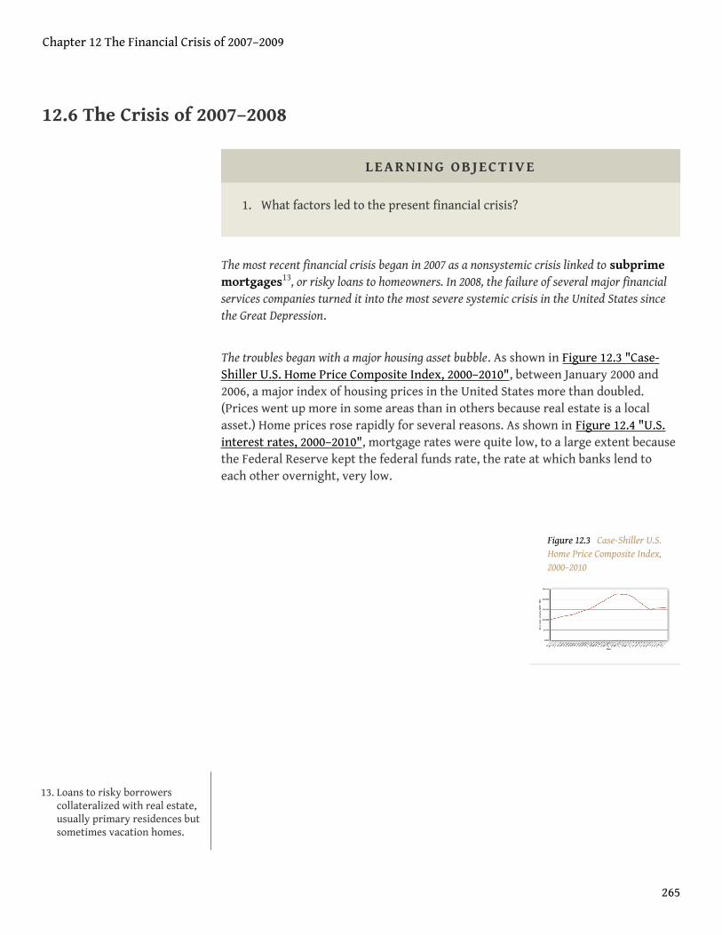
Figure 12.3 Case-Shiller U.S.Home Price Composite Index,2000–2010
12.6 The Crisis of 2007–2008
LEARNING OBJECTIVE
1. What factors led to the present financial crisis?
The most recent financial crisis began in 2007 as a nonsystemic crisis linked to subprimemortgages13, or risky loans to homeowners. In 2008, the failure of several major financialservices companies turned it into the most severe systemic crisis in the United States sincethe Great Depression.
The troubles began with a major housing asset bubble. As shown in Figure 12.3 "Case-Shiller U.S. Home Price Composite Index, 2000–2010", between January 2000 and2006, a major index of housing prices in the United States more than doubled.(Prices went up more in some areas than in others because real estate is a localasset.) Home prices rose rapidly for several reasons. As shown in Figure 12.4 "U.S.interest rates, 2000–2010", mortgage rates were quite low, to a large extent becausethe Federal Reserve kept the federal funds rate, the rate at which banks lend toeach other overnight, very low.
13. Loans to risky borrowerscollateralized with real estate,usually primary residences butsometimes vacation homes.
Chapter 12 The Financial Crisis of 2007–2009
265
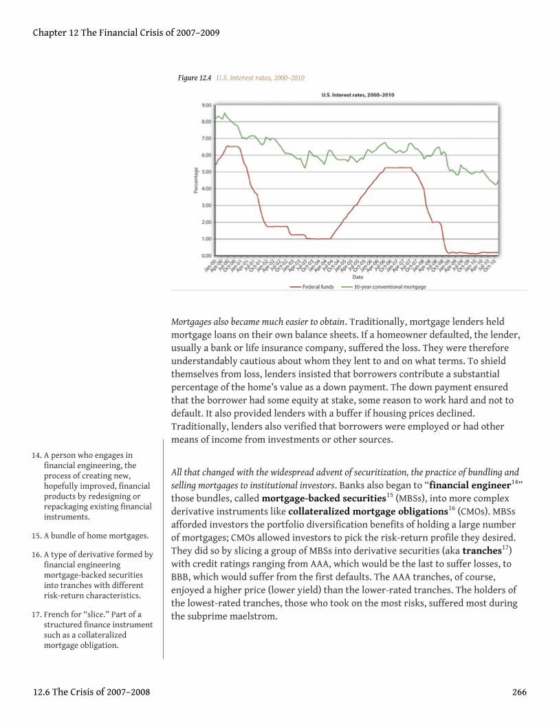
Figure 12.4 U.S. interest rates, 2000–2010
Mortgages also became much easier to obtain. Traditionally, mortgage lenders heldmortgage loans on their own balance sheets. If a homeowner defaulted, the lender,usually a bank or life insurance company, suffered the loss. They were thereforeunderstandably cautious about whom they lent to and on what terms. To shieldthemselves from loss, lenders insisted that borrowers contribute a substantialpercentage of the home’s value as a down payment. The down payment ensuredthat the borrower had some equity at stake, some reason to work hard and not todefault. It also provided lenders with a buffer if housing prices declined.Traditionally, lenders also verified that borrowers were employed or had othermeans of income from investments or other sources.
All that changed with the widespread advent of securitization, the practice of bundling andselling mortgages to institutional investors. Banks also began to “financial engineer14”those bundles, called mortgage-backed securities15 (MBSs), into more complexderivative instruments like collateralized mortgage obligations16 (CMOs). MBSsafforded investors the portfolio diversification benefits of holding a large numberof mortgages; CMOs allowed investors to pick the risk-return profile they desired.They did so by slicing a group of MBSs into derivative securities (aka tranches17)with credit ratings ranging from AAA, which would be the last to suffer losses, toBBB, which would suffer from the first defaults. The AAA tranches, of course,enjoyed a higher price (lower yield) than the lower-rated tranches. The holders ofthe lowest-rated tranches, those who took on the most risks, suffered most duringthe subprime maelstrom.
14. A person who engages infinancial engineering, theprocess of creating new,hopefully improved, financialproducts by redesigning orrepackaging existing financialinstruments.
15. A bundle of home mortgages.
16. A type of derivative formed byfinancial engineeringmortgage-backed securitiesinto tranches with differentrisk-return characteristics.
17. French for “slice.” Part of astructured finance instrumentsuch as a collateralizedmortgage obligation.
Chapter 12 The Financial Crisis of 2007–2009
12.6 The Crisis of 2007–2008 266
Securitization allowed mortgage lenders to specialize in making loans, turningthem more into originators than lenders. Origination was much easier than lendingbecause it required little or no capital. Unsurprisingly, a large number of newmortgage originators, most mere brokers, appeared on the scene. Paid a commissionat closing, originators had little incentive to screen good borrowers from bad and much moreincentive to sign up anyone with a pulse. A race to the bottom occurred as originatorscompeted for business by reducing screening and other credit standards. At theheight of the bubble, loans to no income, no job or assets (NINJA) borrowers werecommon. So-called liars’ loans for hundreds of thousands of dollars were made toborrowers without documenting their income or assets. Instead of insisting on asubstantial down payment, many originators cajoled homeowners into borrowing125 percent of the value of the home because it increased their commissions. Theyalso aggressively pushed adjustable rate mortgages (ARMs) that offered low initialteaser rates and later were reset at much higher levels.
Regulators allowed, and even condoned, such practices in the name of affordable housing,even though six earlier U.S. mortgage securitization schemes had ended badly.KennethSnowden, “Mortgage Securitization in the United States: Twentieth CenturyDevelopments in Historical Perspective,” in Michael Bordo and Richard Sylla, eds.,Anglo-American Financial Systems: Institutions and Markets in the Twentieth Century(Burr Ridge, IL: Irwin Professional Publishing, 1995), 261–298. Regulators alsoallowed Fannie Mae and Freddie Mac, two giant stockholder-owned mortgagesecuritization companies whose debt was effectively guaranteed by the federalgovernment, to take on excessive risks and leverage themselves to the hilt. Theyalso allowed credit-rating agencies to give investment-grade ratings to complicatedmortgage-backed securities of dubious quality. (For the problem with credit-ratingagencies, see Chapter 8 "Financial Structure, Transaction Costs, and AsymmetricInformation".)
Observers, including Yale’s Robert Shillerhttp://www.econ.yale.edu/~shiller/ andStern’s Nouriel Roubini,http://pages.stern.nyu.edu/~nroubini/ warned about theimpending crisis, but few listened. As long as housing prices kept rising, shoddyunderwriting, weak regulatory oversight, and overrated securities were not problemsbecause borrowers who got into trouble could easily refinance or sell the house for a profit.Indeed, many people began to purchase houses with the intention of “flipping”them a month later for a quick buck.
In June 2006, however, housing prices peaked, and by the end of that year it was clear thatthe bubble had gone bye-bye. By summer 2007, prices were falling quickly. Defaultsmounted as the sale/refinance option disappeared, and borrowers wondered whythey should continue paying a $300,000 mortgage on a house worth only $250,000,especially at a time when a nasty increase in fuel costs and a minor bout of inflationstrained personal budgets. Highly leveraged subprime mortgage lenders, like
Chapter 12 The Financial Crisis of 2007–2009
12.6 The Crisis of 2007–2008 267
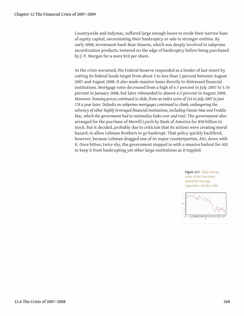
Figure 12.5 Daily closingvalue of the Dow JonesIndustrial Average,September–October 2008
Countrywide and Indymac, suffered large enough losses to erode their narrow baseof equity capital, necessitating their bankruptcy or sale to stronger entities. Byearly 2008, investment bank Bear Stearns, which was deeply involved in subprimesecuritization products, teetered on the edge of bankruptcy before being purchasedby J. P. Morgan for a mere $10 per share.
As the crisis worsened, the Federal Reserve responded as a lender of last resort bycutting its federal funds target from about 5 to less than 2 percent between August2007 and August 2008. It also made massive loans directly to distressed financialinstitutions. Mortgage rates decreased from a high of 6.7 percent in July 2007 to 5.76percent in January 2008, but later rebounded to almost 6.5 percent in August 2008.Moreover, housing prices continued to slide, from an index score of 216 in July 2007 to just178 a year later. Defaults on subprime mortgages continued to climb, endangering thesolvency of other highly leveraged financial institutions, including Fannie Mae and FreddieMac, which the government had to nationalize (take over and run). The government alsoarranged for the purchase of Merrill Lynch by Bank of America for $50 billion instock. But it decided, probably due to criticism that its actions were creating moralhazard, to allow Lehman Brothers to go bankrupt. That policy quickly backfired,however, because Lehman dragged one of its major counterparties, AIG, down withit. Once bitten, twice shy, the government stepped in with a massive bailout for AIGto keep it from bankrupting yet other large institutions as it toppled.
Chapter 12 The Financial Crisis of 2007–2009
12.6 The Crisis of 2007–2008 268
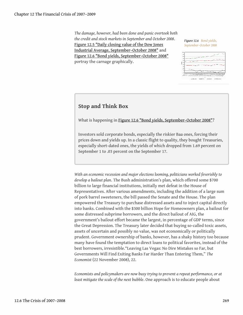
Figure 12.6 Bond yields,September–October 2008
The damage, however, had been done and panic overtook boththe credit and stock markets in September and October 2008.Figure 12.5 "Daily closing value of the Dow JonesIndustrial Average, September–October 2008" andFigure 12.6 "Bond yields, September–October 2008"portray the carnage graphically.
Stop and Think Box
What is happening in Figure 12.6 "Bond yields, September–October 2008"?
Investors sold corporate bonds, especially the riskier Baa ones, forcing theirprices down and yields up. In a classic flight to quality, they bought Treasuries,especially short-dated ones, the yields of which dropped from 1.69 percent onSeptember 1 to .03 percent on the September 17.
With an economic recession and major elections looming, politicians worked feverishly todevelop a bailout plan. The Bush administration’s plan, which offered some $700billion to large financial institutions, initially met defeat in the House ofRepresentatives. After various amendments, including the addition of a large sumof pork barrel sweeteners, the bill passed the Senate and the House. The planempowered the Treasury to purchase distressed assets and to inject capital directlyinto banks. Combined with the $300 billion Hope for Homeowners plan, a bailout forsome distressed subprime borrowers, and the direct bailout of AIG, thegovernment’s bailout effort became the largest, in percentage of GDP terms, sincethe Great Depression. The Treasury later decided that buying so-called toxic assets,assets of uncertain and possibly no value, was not economically or politicallyprudent. Government ownership of banks, however, has a shaky history too becausemany have found the temptation to direct loans to political favorites, instead of thebest borrowers, irresistible.“Leaving Las Vegas: No Dire Mistakes so Far, butGovernments Will Find Exiting Banks Far Harder Than Entering Them,” TheEconomist (22 November 2008), 22.
Economists and policymakers are now busy trying to prevent a repeat performance, or atleast mitigate the scale of the next bubble. One approach is to educate people about
Chapter 12 The Financial Crisis of 2007–2009
12.6 The Crisis of 2007–2008 269
bubbles in the hope that they will be more cautious investors. Another is toencourage bank regulators to use their powers to keep leverage to a minimum. Athird approach is to use monetary policy—higher interest rates or tighter moneysupply growth—to deflate bubbles before they grow large enough to endanger theentire financial system. Each approach has its strengths and weaknesses. Educationmight make investors afraid to take on any risk. Tighter regulation and monetarypolicy might squelch legitimate, wealth-creating industries and sectors. Acombination of better education, more watchful regulators, and lessaccommodative monetary policy may serve us best.
KEY TAKEAWAYS
• Low interest rates, indifferent regulators, unrealistic credit ratings forcomplex mortgage derivatives, and poor incentives for mortgageoriginators led to a housing bubble that burst in 2006.
• As housing prices fell, homeowners with dubious credit and negativeequity began to default in unexpectedly high numbers.
• Highly leveraged financial institutions could not absorb the losses andhad to shut down or be absorbed by stronger institutions.
• Despite the Fed’s efforts as lender of last resort, the nonsystemic crisisbecame systemic in September 2008 following the failure of LehmanBrothers and AIG.
• The government responded with huge bailouts of subprime mortgageholders and major financial institutions.
Chapter 12 The Financial Crisis of 2007–2009
12.6 The Crisis of 2007–2008 270
12.7 Suggested Reading
Ben-Shahard, Danny, Charles Ka Yui Leung, and Seow Eng Ong. Mortgage MarketsWorldwide. Hoboken, NJ: John Wiley and Sons, 2007.
Kindleberger, Charles, and Robert Aliber. Manias, Panics, and Crashes: A History ofFinancial Crises, 5th ed. Hoboken, NJ: John Wiley and Sons, 2005.
Mishkin, Frederic. “How Should We Respond to Asset Price Bubbles?” in Banque deFrance, Financial Stability Review. October 2008, 65–74.
Reinhart, Carmen, and Kenneth Rogoff. This Time Is Different: Eight Centuries ofFinancial Folly. Princeton: Princeton University Press, 2009.
Roubini, Nouriel, and Brad Stetser. Bailouts or Bail-ins: Responding to Financial Crises inEmerging Markets. New York: Peterson Institute, 2004.
Shiller, Robert. Irrational Exuberance. New York: Doubleday, 2006.
The Subprime Solution: How Today’s Global Financial Crisis Happened, and What to DoAbout It. Princeton, NJ: Princeton University Press, 2008.
Sprague, Irvine. Bailout: An Insider’s Account of Bank Failures and Rescues. New York:Beard Books, 2000.
Wright, Robert E., ed. Bailouts: Public Money, Private Profit. New York: ColumbiaUniversity Press, 2010.
Chapter 12 The Financial Crisis of 2007–2009
271
Chapter 13
Central Bank Form and Function
CHAPTER OBJECTIVES
By the end of this chapter, students should be able to:
1. Define central bank and explain the importance of central banking.2. Briefly sketch the history of U.S. central banking.3. Explain when and how a country can do without a central bank.4. Briefly sketch the structure of the Federal Reserve System.5. Explain how other central banks compare to the Fed.6. Define central bank independence and explain its importance.7. Explain why independent central bankers prefer lower inflation rates
than government officials do.
272
13.1 America’s Central Banks
LEARNING OBJECTIVES
1. What is a central bank?2. Why is central banking important?3. How can a country manage without a central bank?4. What is the history of central banking in the United States?
A central bank1 is a bank under some degree of government control that isgenerally charged with
• controlling the money supply (to a greater or lesser degree);• providing price stability (influencing the price level);• attaining economic output and employment goals;• regulating commercial banks (and perhaps other depository and
nondepository financial institutions);• stabilizing the macroeconomy (proactively and/or by acting as a
lender of last resort during financial crises);• providing a payments system (check clearing and long-distance
payments).
Central banks also often act as the national government’s banker by holding itsdeposits and making payments on its behalf. During its 200-plus-year existence, theUnited States has had three different central banks and two periods, one short and oneextremely long, with no central bank.
Chartered by the federal government in 1791, the Bank of the United States (BUS)worked in conjunction with the U.S. Treasury secretary to act as a lender of lastresort and a regulator of commercial banks. Specifically, it helped AlexanderHamilton, America’s first Secretary of the Treasury,http://www.treasury.gov/about/history/Pages/ahamilton.aspx to stymie the Panic of 1792. It also returned thenotes of commercial banks for redemption into gold and silver (the era’s base money2),thereby regulating commercial banks’ reserve ratios and hence the money supply. Ownedby private shareholders, the BUS was quite independent, a good trait for a central bank tohave, as we’ll see. Its very independence and power to regulate commercial banks,however, made it unpopular in some influential political circles. Its charter was notrenewed when it expired in 1811. The government’s difficulties financing the Warof 1812 (aka the Second War for Independence) convinced many that the country
1. A bank that regulates themoney supply, interest rates,and/or other financialinstitutions on behalf of thegovernment.
2. The most elementary form ofmoney in a given society at agiven time. The only type ofmoney that can compose abank’s primary reserve.
Chapter 13 Central Bank Form and Function
273
needed a new central bank. As a result, the government chartered the Bank of theUnited States (informally called the Second Bank or SBUS) in 1816. Insufficientlyindependent of the government at first, the SBUS, which (like the BUS) washeadquartered in Philadelphia but had more numerous branches, stumbled byallowing commercial banks to increase their lending too much. It also suffered frominternal agency problems, particularly at its branch in Baltimore. When a financialpanic struck in late 1818 and early 1819, it failed to prevent a recession and debtdeflation. (Sound familiar? See the discussion of the Great Depression in Chapter 11"The Economics of Financial Regulation".) Private stockholders reasserted controlover the bank, placing it under the able direction of Nicholas Biddle, whosuccessfully prevented the British economic meltdown of 1825 from spreading toAmerica. Under Biddle, the SBUS also became an effective regulator of the nation’scommercial banks, which by the 1820s numbered in the hundreds. Like the BUSbefore it, the SBUS paid for its diligence with its life. Aided by many commercialbankers, particularly those in Philadelphia’s financial rival Manhattan, andAmerica’s traditional distaste for powerful institutions, Andrew Jackson vetoed theact rechartering it. (The SBUS continued its corporate life under a Pennsylvaniacharter, but it no longer had nationwide branches and was no longer the nation’scentral bank. It went bankrupt a few years later.)
From 1837 until late 1914, the United States had no central bank. Private institutionscropped up to clear checks and transfer funds over long distances. The Treasurykept its funds in commercial banks and in the hands of its tax collectors and leftbank regulation to the market (deposit and note holders and stockholders) andstate governments. The monetary base (gold and silver) it left largely to the whimsof international trade. It could do so because the United States and most of theworld’s other major economies were on a gold and/or silver standard, meaning thattheir respective units of account were fixed in terms of so many grains of theprecious stuff and hence fixed against each other.This does not mean that theexchange rate didn’t change, merely that it stayed within a narrow band oftransaction costs. As we’ll learn in Chapter 18 "Foreign Exchange", the system wasself-equilibrating. In other words, discretionary monetary policy was unnecessarybecause gold and silver flowed into or out of economies automatically, as needed.Nations today that maintain fixed exchange rates also find no need for a centralbank, but instead use a simpler institution called a currency board. Countries thatuse a foreign currency as their own, a process called dollarization3, need nothingat all because they essentially outsource their monetary policy to the central bankof the nation whose currency they use. (That is often the United States, hence theterm dollarization.) Other central banking functions, like clearing checks andregulating financial institutions, can be performed by other entities, public andprivate. The function of lender of last resort typically cannot be fulfilled, however,by anything other than a central bank.
3. The process of using a foreigncountry’s money as a domesticcurrency. Often this entails acountry adopting the U.S.dollar as a medium of exchangeand unit of account.
Chapter 13 Central Bank Form and Function
13.1 America’s Central Banks 274
Indeed, the biggest problem with the U.S. arrangement was that there was no officialsystemwide lender of last resort, nobody to increase the money supply or lower interest ratesin the face of a shock. As a result, the United States suffered from banking crises andfinancial panics of increasing ferocity beginning soon after the Second Bank’sdemise: 1837, 1839, 1857, 1873, 1884, 1893, and 1907. Most of those panics werefollowed by recessions and debt deflation because there was no institution wealthyenough to stop the death spiral described in Chapter 12 "The Financial Crisis of2007–2009" and in Chapter 23 "Aggregate Supply and Demand, the GrowthDiamond, and Financial Shocks" (a shock, increased asymmetric information,decline in economic activity, bank panic, increased asymmetric information,decline in economic activity, unanticipated decline in the price level). In 1907, J. P.Morgan (the man, with help from his bank and web of business associates)mitigated, but did not prevent, a serious recession by acting as a lender of lastresort. The episode convinced many Americans that the time had come to create anew central bank lest private financiers come to wield too much power. Anyonewith the power to stop a panic, they reasoned, had the power to start one.Americans still feared powerful government institutions too, however, so it tookanother six years (1913) to agree on the new bank’s structure, which was highlydecentralized geographically and chock full of checks and balances. It took anotheryear (1914) to get the bank, often called simply the Fed or the Federal Reserve, intooperation. We’ll discuss the checkered history of the Fed’s monetary policy inChapter 17 "Monetary Policy Targets and Goals".
Chapter 13 Central Bank Form and Function
13.1 America’s Central Banks 275
KEY TAKEAWAYS
• A central bank is a bank under some degree of government control thatis responsible for influencing the money supply, interest rates, inflation,and other macroeconomic outcomes like output and employment. Acentral bank is usually the lender of last resort, the institution that can(and should) add liquidity and confidence to the financial system at theoutbreak of panics and crises. On a quotidian basis, central banks alsomay clear checks, regulate banks and/or other financial institutions,and serve as the national government’s bank.
• Early in its history, the United States was home to two privately ownedcentral banks, the Bank of the United States and the Second Bank, thatacted as a lender of last resort and regulated commercial banks byreturning their notes to them for redemption in base money (then goldand silver). Although economically effective, both were politicallyunpopular so when their twenty-year charters expired, they were notrenewed. From 1837 until the end of 1914, the United States had nocentral bank, but the Treasury Department fulfilled some of itsfunctions.
• A country can do without a central bank if it is on fixed exchange rates,such as the gold standard, or otherwise gives up discretionary monetarypolicy, as when countries dollarize or adopt a foreign currency as theirown. In such cases, other institutions fulfill central banking functions:government departments regulate financial institutions, commercialbanks safeguard the government’s deposits, a currency boardadministers the fixed exchange rate mechanism, clearinghousesestablished by banks clear checks, and so forth.
• The Treasury Department did not act as a lender of last resort, however,so recurrent banking crises and financial panics plagued the economy.When J. P. Morgan acted as a lender of last resort during the Panic of1907, political sentiments shifted and the Federal Reserve systememerged out of a series of political compromises six years later.
Chapter 13 Central Bank Form and Function
13.1 America’s Central Banks 276
13.2 The Federal Reserve System’s Structure
LEARNING OBJECTIVE
1. What is the structure of the Federal Reserve system?
The Federal Reserve is composed of twelve numbered districts, each with its own FederalReserve Bank: Boston (1), New York (2), Philadelphia (3), Cleveland (4), Richmond (5),Atlanta (6), Chicago (7), St. Louis (8), Minneapolis (9), Kansas City (10), Dallas (11),and San Francisco (12). Except for regions 1 and 3, each of those district banks4
also operates one or more branches. For example, the Federal Reserve Bank of NewYork (FRBNY) maintains a branch in Buffalo; the Atlanta Fed has branches inNashville, Birmingham, New Orleans, Jacksonville, and Miami. The Fed’sheadquarters is located in Washington, DCFor an interactive map of the system,browse http://www.federalreserve.gov/otherfrb.htm.
Missouri is the only state with two federal reserve district banks. This was thoughtnecessary to secure the votes of Missouri congressional representatives for the bill.(So much for public interest!) The districts don’t seem to be evenly balancedeconomically. They were, more or less, when the legislation was passed before WorldWar I, but since then, the West Coast, Southwest, and Southeast (Sunbelt) havegrown in economic importance relative to the Northeast and old Midwest(Rustbelt). (District 3 encompasses only southern New Jersey and easternPennsylvania, an area that is no longer the economic powerhouse it once was.)Rather than redistrict, the Fed has simply shifted resources over the years towardthe larger and economically more potent districts.
Each Federal Reserve bank is owned by the commercial banks in its district, and they aremembers of the system. Those banks, which include all nationally chartered banksand any state banks that choose to join, own restrictedThe Fed’s stock is not tradedin public markets and pays an annual dividend no higher than 6 percent. shares inthe Fed, which they use to elect six directors, three of whom have to be professionalbankers and three of whom have to be nonbank business leaders. The Board ofGovernors in Washington selects another three directors, who are supposed torepresent the public interest and are not allowed to work for or own stock in anybank. The nine directors, with the consent of the board, then appoint a president.
The twelve district banks do mostly grunt work:4. One of the twelve banks
comprising the Federal Reservesystem.
Chapter 13 Central Bank Form and Function
277
• Issue new Federal Reserve notes (FRNs) in place of worn currency• Clear checks• Lend to banks within their districts• Act as a liaison between the Fed and the business community• Collect data on regional business and economic conditions• Conduct monetary policy research• Evaluate bank merger and new activities applications• Examine bank holding companies and state-chartered member
banks.The Comptroller of the Currency is the primary regulator offederally chartered banks. State regulators and the FDIC regulate statebanks that are not members of the Federal Reserve system.
The FRBNY is the most important of the district banks because, in addition to the tasks listedabove, it also conducts so-called open market operations, buying and selling governmentbonds (and occasionally other assets) on behalf of the Federal Reserve system and at thebehest of headquarters in Washington. Moreover, the FRBNY is a member of the Bankfor International Settlements (BIS)http://www.bis.org/ and safeguards over $100billion in gold owned by the world’s major central banks. Finally, the FRBNY’spresident is the only permanent member of the Federal Open Market Committee(FOMC).
The FOMC is composed of the seven members of the Board of Governors, the president of theFRBNY, and the presidents of the other district banks, though only four of the last-mentionedgroup can vote (on a rotating basis). The FOMC meets every six weeks or so to decideon monetary policy, specifically on the rate of growth of the money supply or thefederal funds target rate, an important interest rate, both of which are controlledvia so-called open market operations. Until recently, the Fed had only two othertools for implementing monetary policy, the discount rate at which district bankslend directly to member banks and reserve requirements. Prior to the crisis of2007–2008, neither was an effective tool for a long time, so the market and themedia naturally concentrated on the FOMC and have even taken to calling it “theFed,” although technically it is only one part of the giant beast. The head of the Fed isthe Board of Governors, which is composed of a chairperson, currently Ben Bernanke, and sixgovernors.http://www.federalreserve.gov/aboutthefed/bios/board/bernanke.htmAll seven are appointed by the president of the United States and confirmed by theU.S. Senate. The governors must come from different Federal Reserve districts andserve a single fourteen-year term. The chairperson is selected from among thegovernors and serves a four-year, renewable term. The chairperson is the mostpowerful member of the Fed because he or she controls the board, which controlsthe FOMC, which controls the FRBNY’s open market operations, which influencesthe money supply or a key interest rate. The chairperson also effectively controlsreserve requirements and the discount rate. He (so far no women) is also the Fed’spublic face and its major liaison to the national government. Although de jure
Chapter 13 Central Bank Form and Function
13.2 The Federal Reserve System’s Structure 278
power within the Fed is diffused by the checks and balances discussed above, todayde facto power is concentrated in the chairperson. That allows the Fed to beeffective but ensures that a rogue chairperson cannot abuse his power.
Historically, some chairpersons have made nebbishes look effective, while others,including most recently Alan Greenspan, have been considered, if not infallibledemigods, then at least erudite gurus. Neither extreme view is accurate because allchairpersons have relied heavily on the advice and consent of the other governors, thedistrict banks’ presidents, and the Fed’s research staff of economists, which is the world’slargest. The researchers provide the chairperson and the entire FOMC with newdata, qualitative assessments of economic trends, and quantitative output from thelatest and greatest macroeconomic models. They also examine the global economyand analyze the foreign exchange market, on the lookout for possible shocks fromabroad. Fed economists also help the district banks to do their jobs by investigatingmarket and competition conditions and engaging in educational and other publicoutreach programs.
KEY TAKEAWAYS
• The Fed is composed of a Washington-based headquarters and twelvedistrict banks and their branches.
• The district banks, which are owned by the member banks, fulfill theFed’s quotidian duties like clearing checks and conducting economicresearch.
• The most important of the district banks is the Federal Reserve Bank ofNew York (FRBNY), which conducts open market operations, the buyingand selling of bonds that influences the money supply and interest rates.
• It also safeguards much of the world’s gold and has a permanent seat onthe Federal Open Market Committee (FOMC), the Fed’s most importantpolicymaking body.
• Composed of the Board of Governors and the presidents of the districtbanks, the FOMC meets every six weeks or so to decide whethermonetary policy should be tightened (interest rates increased), loosened(interest rates decreased), or maintained.
• The Fed is full of checks and balances, but is clearly led by thechairperson of the Board of Governors.
• The chairperson often personifies the Fed as he (to date it’s been a male)is the bank’s public face.
• Nevertheless, a large number of people, from common businesspeople tothe Fed’s research economists, influence his decisions through the data,opinions, and analysis they present.
Chapter 13 Central Bank Form and Function
13.2 The Federal Reserve System’s Structure 279
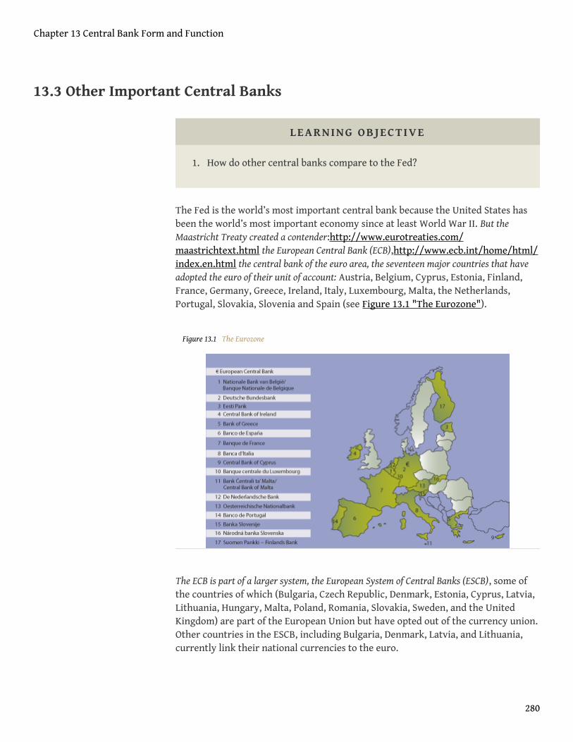
13.3 Other Important Central Banks
LEARNING OBJECTIVE
1. How do other central banks compare to the Fed?
The Fed is the world’s most important central bank because the United States hasbeen the world’s most important economy since at least World War II. But theMaastricht Treaty created a contender:http://www.eurotreaties.com/maastrichtext.html the European Central Bank (ECB),http://www.ecb.int/home/html/index.en.html the central bank of the euro area, the seventeen major countries that haveadopted the euro of their unit of account: Austria, Belgium, Cyprus, Estonia, Finland,France, Germany, Greece, Ireland, Italy, Luxembourg, Malta, the Netherlands,Portugal, Slovakia, Slovenia and Spain (see Figure 13.1 "The Eurozone").
Figure 13.1 The Eurozone
The ECB is part of a larger system, the European System of Central Banks (ESCB), some ofthe countries of which (Bulgaria, Czech Republic, Denmark, Estonia, Cyprus, Latvia,Lithuania, Hungary, Malta, Poland, Romania, Slovakia, Sweden, and the UnitedKingdom) are part of the European Union but have opted out of the currency union.Other countries in the ESCB, including Bulgaria, Denmark, Latvia, and Lithuania,currently link their national currencies to the euro.
Chapter 13 Central Bank Form and Function
280
The ECB or Eurosystem was consciously modeled on the Fed, so it is not surprising that theirstructures are similar. Each nation is like a Federal Reserve district headed by itsnational central bank (NCB). At its headquarters in Frankfurt sits the ECB’sExecutive Board, the structural equivalent of the Fed’s Board of Governors, and theGoverning Council, which like the Fed’s FOMC makes monetary policy decisions.The ECB is more decentralized than the Fed, however, because the NCBs controltheir own budgets and conduct their own open market operations. Also unlike theFed, the ECB does not regulate financial institutions, a task left to each individualcountry’s government. The two central banks, of course, also differ in many mattersof detail. The ECB’s current head or president is a Frenchman named Jean-ClaudeTrichet.http://en.wikipedia.org/wiki/President_of_the_European_Central_Bank#Trichet
Three other important central banks, the Bank of England, the Bank of Japan, andthe Bank of Canada, look nothing like the Fed or the ECB because they are unitaryinstitutions with no districts. Although they are more independent than in the past, mostare not as independent as the Fed or the ECB. Despite their structural differences andrelative dearth of independence, unit central banks like the Bank of Japanimplement monetary policy in ways very similar to the Fed and ECB.DieterGerdesmeier, Francesco Mongelli, and Barbara Roffia, “The Eurosystem, the USFederal Reserve and the Bank of Japan: Similarities and Differences,” ECB WorkingPaper Series No. 742 (March 2007).
KEY TAKEAWAY
• The European Central Bank (ECB), the central bank of the nations thathave adopted the euro, and the larger European System of Central Banks(ECSB), of which it is a part, are modeled after the Fed. Nevertheless,numerous differences of detail can be detected. The ECB’s nationalcentral banks (NCBs), for example, are much more powerful than theFed’s district banks because they control their own budgets and conductopen market operations. Most of the world’s other central banks arestructured differently than the ECB and the Fed because they are unitbanks without districts or branches. Most are less independent than theFed and ECB but conduct monetary policy in the same ways.
Chapter 13 Central Bank Form and Function
13.3 Other Important Central Banks 281
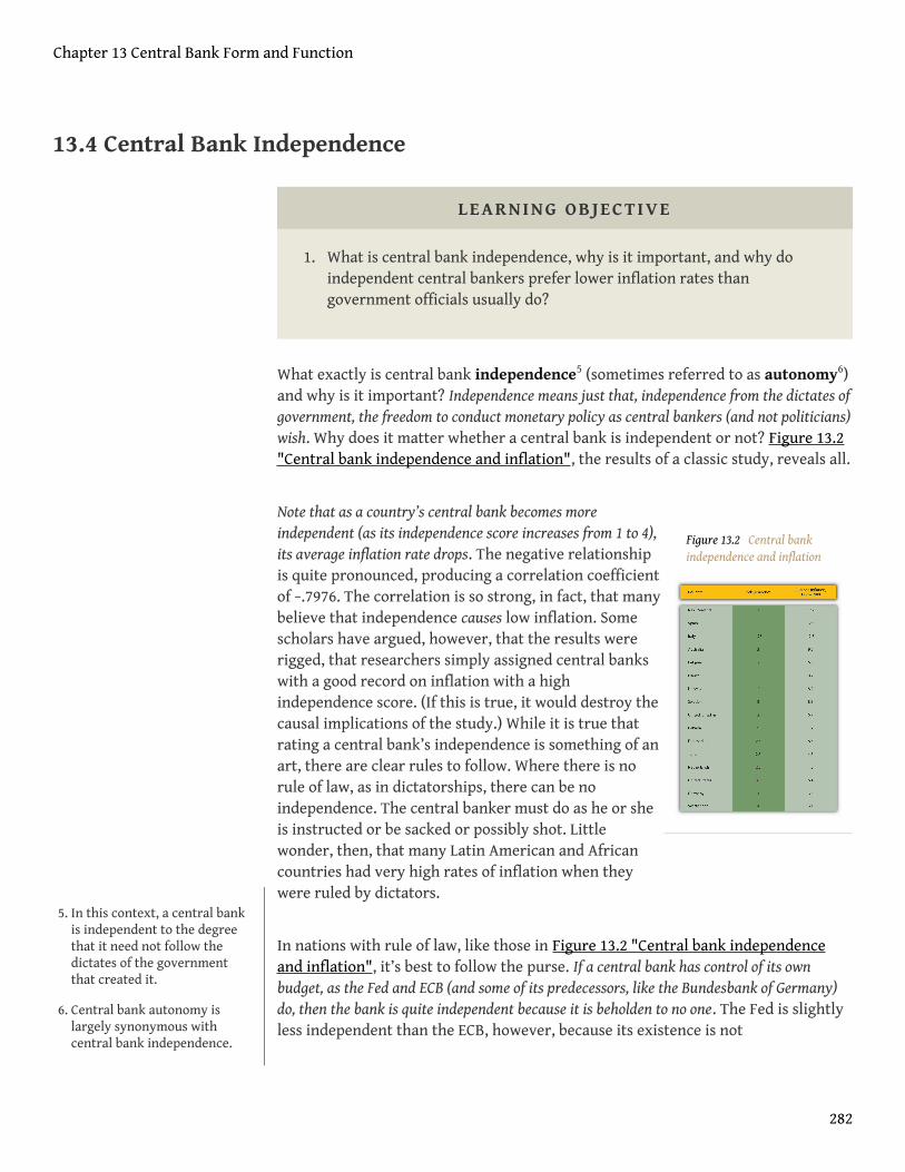
Figure 13.2 Central bankindependence and inflation
13.4 Central Bank Independence
LEARNING OBJECTIVE
1. What is central bank independence, why is it important, and why doindependent central bankers prefer lower inflation rates thangovernment officials usually do?
What exactly is central bank independence5 (sometimes referred to as autonomy6)and why is it important? Independence means just that, independence from the dictates ofgovernment, the freedom to conduct monetary policy as central bankers (and not politicians)wish. Why does it matter whether a central bank is independent or not? Figure 13.2"Central bank independence and inflation", the results of a classic study, reveals all.
Note that as a country’s central bank becomes moreindependent (as its independence score increases from 1 to 4),its average inflation rate drops. The negative relationshipis quite pronounced, producing a correlation coefficientof −.7976. The correlation is so strong, in fact, that manybelieve that independence causes low inflation. Somescholars have argued, however, that the results wererigged, that researchers simply assigned central bankswith a good record on inflation with a highindependence score. (If this is true, it would destroy thecausal implications of the study.) While it is true thatrating a central bank’s independence is something of anart, there are clear rules to follow. Where there is norule of law, as in dictatorships, there can be noindependence. The central banker must do as he or sheis instructed or be sacked or possibly shot. Littlewonder, then, that many Latin American and Africancountries had very high rates of inflation when theywere ruled by dictators.
In nations with rule of law, like those in Figure 13.2 "Central bank independenceand inflation", it’s best to follow the purse. If a central bank has control of its ownbudget, as the Fed and ECB (and some of its predecessors, like the Bundesbank of Germany)do, then the bank is quite independent because it is beholden to no one. The Fed is slightlyless independent than the ECB, however, because its existence is not
5. In this context, a central bankis independent to the degreethat it need not follow thedictates of the governmentthat created it.
6. Central bank autonomy islargely synonymous withcentral bank independence.
Chapter 13 Central Bank Form and Function
282
constitutionally guaranteed. (Indeed, as we learned above, the United States had anasty habit of dispatching its early central banks.) Congress could change or abolishthe Fed simply by passing a law and getting the president to sign it or it couldoverride his veto. The ECB, by contrast, was formed by an international treaty,changes to which must be ratified by all the signatories, a chore and a half toachieve, to be sure! Finally, central banks led by people who are appointed are moreindependent than those led by popularly elected officials. Long, nonrenewable terms arebetter for independence than short, renewable ones, which tend to induce bankers to currythe favor of whoever decides their fate when their term expires.
None of this is to say, however, that determining a central bank’s independence iseasy, particularly when de jure and de facto realities differ. The Bank of Canada’sindependence is limited by the fact that the Bank Act of 1967 made the governmentultimately responsible for Canada’s monetary policy. But, in fact, the Canadiangovernment has allowed its central bank to run the money show. The same could besaid of the Bank of England. The Bank of Japan’s independence was strengthened in1998 but the Ministry of Finance, a government agency, still controls part of itsbudget and can request delays in monetary policy decisions. The current de factoindependence of those banks could be undermined and quite quickly at that.
Stop and Think Box
“Bank of Japan Faces Test of Independence,” Wall Street Journal, August 10,2000.“The political storm over a possible interest rate increase by the Bank ofJapan is shaping up to be the biggest challenge to the central bank’sindependence since it gained autonomy two years ago. Members of the rulingLiberal Democratic Party stepped up pressure on the bank to leave thecountry’s interest rates where they are now.” Why does the Liberal DemocraticParty (LDP) want to influence the Bank of Japan’s (BoJ’s) interest rate policy?Why was the issue important enough to warrant a major article in a majorbusiness newspaper?
The LDP wanted to influence the BoJ’s interest rate policy for political reasons,namely, to keep the economy from slowing, a potential threat to its rule. Thiswas an important story because the de facto “independence” of the BoJ was atstake and hence the market’s perception of the Japanese central bank’s abilityto raise interest rates to stop inflation in the face of political pressure.
Chapter 13 Central Bank Form and Function
13.4 Central Bank Independence 283
Why, when left to their own devices, are central bankers tougher on inflation thangovernments, politicians, or the general populace? Partly because they represent bank,business, and creditor interests, all of which are hurt if prices rise quickly andunexpectedly. We learned in Chapter 9 "Bank Management" that banks arenaturally uncomfortable in rising interest rate environments, and in Chapter 4"Interest Rates", we saw that inflation invariably brings with it higher rates. Netcreditors—economic entities that are owed more than they owe—also dislikeinflation because it erodes the real value of the money owed them. Finally,businesses tend to dislike inflation because it increases uncertainty and makeslong-term planning difficult. Central bankers also know the damage that inflationcan do to an economy, so a public interest motivation drives them as well.
People and the politicians they elect to office, on the other hand, often desire inflation. Manyhouseholds are net debtors, meaning that they owe more money than is owed tothem. Inflation, they know, will decrease the real burden of their debts. Politiciansknow this, too, so they tend to err on the side of higher rather than lower inflation.Politicians also know that monetary stimulus—increasing the money supply at afaster rate than usual or lowering the interest rate—can stimulate a short burst ofeconomic growth that will make people happy with the status quo and ready toreturn incumbents to office. If inflation ensues and the economy turns sour forawhile after the election, that is okay because matters will likely sort out before thenext election, when politicians will be again inclined to pump out money. This iscalled the political business cycle. Politicians might also want to print money simply toavoid raising direct taxes. The resultant inflation acts like a tax on cash balances(which lose value each day) and blame can be cast on the central bankers.
All in all, then, it is a good idea to have a central bank with a good deal of independence,thoughsome liberals complain that independent central banks aren’t sufficiently“democratic.” But who says everything should be democratic? Would you want thearmed forces run by majority vote? Your company? Your household? Have youheard about the tyranny of the majority?http://xroads.virginia.edu/~hyper/detoc/1_ch15.htm That’s when two wolves and a sheep vote on what’s for dinner. Centralbank independence is not just about inflation but about how well the overalleconomy performs. There is no indication that the inflation fighting done byindependent central banks in any way harms economic growth or employment inthe long run. Keeping the lid on inflation, which can seriously injure nationaleconomies, is therefore a very good policy indeed.
Another knock against independent central banks is that they are not verytransparent. The Fed, for example, has long been infamous for its secrecy. Whenforced by law to disclose more information about its actions sooner, it turned toobfuscation. To this day, decoding the FOMC’s press releases is an interesting gameof semantics. For all its unclear language, the Fed is more open than the ECB, which
Chapter 13 Central Bank Form and Function
13.4 Central Bank Independence 284
will not make the minutes of its policy meetings public until twenty years after theytake place. It is less transparent, however, than many central banks that publishtheir economic forecasts and inflation rate targets. As we will see in Chapter 26"Rational Expectations Redux: Monetary Policy Implications", theory suggests thatcentral banks should be transparent when trying to stop inflation but opaque whentrying to stimulate the economy.
KEY TAKEAWAYS
• Central bank independence is a measure of how free from governmentinfluence central bankers are. Independence increases as a central bankcontrols its own budget; it cannot be destroyed or modified by merelegislation (or, worse, executive fiat), and it is enhanced when centralbanks are composed of people serving long, nonrenewable terms.Independence is important because researchers have found that themore independent a central bank is, the lower the inflation it allowswithout injuring growth and employment goals.
• When unanticipated, inflation redistributes resources from net creditorsto net debtors, creates uncertainty, and raises nominal interest rates,hurting economic growth.
• Independent central bankers represent bank, business, and net creditorinterests that are hurt by high levels of inflation. Elected officialsrepresent voters, many of whom are net debtors, and hencebeneficiaries of debt-eroding inflationary measures.
• They also know that well-timed monetary stimulus can help them obtainre-election by inducing economic growth in the months leading up tothe election. The inflation that follows will bring some pain, but therewill be time for correction before the next election. Governments whereofficials are not elected, as in dictatorships, often have difficultycollecting taxes, so they use the central bank as a source of revenue,simply printing money (creating bank deposits) to make payments. Highlevels of inflation act as a sort of currency tax, a tax on cash balancesthat lose some of their purchasing power each day.
Chapter 13 Central Bank Form and Function
13.4 Central Bank Independence 285
13.5 Suggested Reading
Bremner, Robert. Chairman of the Fed: William McChesney Martin Jr. and the Creation ofthe American Financial System. New Haven, CT: Yale University Press, 2004.
Bruner, Robert, and Sean Carr. The Panic of 1907: Lessons Learned from the Market’sPerfect Storm. Hoboken, NJ: John Wiley and Sons, 2007.
Clark, William Roberts. Capitalism, Not Globalismml: Capital Mobility, Central BankIndependence, and the Political Control of the Economy. Ann Arbor, MI: University ofMichigan Press, 2005.
Meltzer, Allan. A History of the Federal Reserve, Volume 1: 1913–1951. Chicago, IL:University of Chicago Press, 2003.
Timberlake, Richard. Monetary Policy in the United States: An Intellectual andInstitutional History. Chicago, IL: University of Chicago Press, 1993.
Chapter 13 Central Bank Form and Function
286
Chapter 14
The Money Supply Process
CHAPTER OBJECTIVES
By the end of this chapter, students should be able to:
1. Describe who determines the money supply.2. Explain how the central bank’s balance sheet differs from the balance
sheets of commercial banks and other depository institutions.3. Define the monetary base and explain its importance.4. Define open market operations and explain how they affect the
monetary base.5. Describe the multiple deposit creation process.6. Define the simple deposit multiplier and explain its information
content.7. List and explain the two major limitations or assumptions of the simple
deposit multiplier.
287
14.1 The Central Bank’s Balance Sheet
LEARNING OBJECTIVES
1. Who determines the money supply?2. How does the central bank’s balance sheet differ from the balance sheets
of other banks?3. What is the monetary base?
Ultimately the money supply is determined by the interaction of four groups: commercialbanks and other depositories, depositors, borrowers, and the central bank. Like any bank,the central bank’s balance sheet is composed of assets and liabilities. Its assets aresimilar to those of common banks and include government securitiesStudentssometimes become confused about this because they think the central bank is thegovernment. At most, it is part of the government, and not the part that issues thebonds. Sometimes, as in the case of the BUS and SBUS, it is not part of thegovernment at all. and discount loans. The former provide the central bank withincome and a liquid asset that it can easily and cheaply buy and sell to alter itsbalance sheet. The latter are generally loans made to commercial banks. So far, sogood. The central bank’s liabilities, however, differ fundamentally from those of commonbanks. Its most important liabilities are currency in circulation and reserves.
Yes, currency and reserves. You may recall from Chapter 9 "Bank Management"that those are the assets of commercial banks. In fact, for everyone but the central bank,the central bank’s notes, Federal Reserve notes (FRN) in the United States, are assets, thingsowned. But for the central bank, its notes are things owed (liabilities), just like yourpromissory note (IOU) would be your liability, but it would be an asset for the note’sholder or owner. Similarly, commercial banks own their deposits in the Fed(reserves), which the Fed, of course, owes to the commercial banks. So reserves arecommercial bank assets but central bank liabilities.
Currency in circulation (C) and reserves (R) compose the monetary base1(MB, aka high-powered money), the most basic building blocks of the money supply. Basically, MB = C + R,an equation you’ll want to internalize. In the United States, C includes FRN andcoins issued by the U.S. Treasury. We can ignore the latter because it is a relativelysmall percentage of the MB, and the Treasury cannot legally manage the volume ofcoinage in circulation in an active fashion, but rather only meets the demand foreach denomination: .01, .05, .10, .25, .50, and 1.00 coins. (The Fed also supplies the$1.00 unit, and for some reason Americans prefer $1 notes to coins. In most
1. The most basic, powerful typesof money in a given monetarysystem, that is, gold and silverunder the gold standard, FRN,and reserves (Federal Reservedeposits) today.
Chapter 14 The Money Supply Process
288
countries, coins fill demand for the single currency unit denomination.) C includesonly FRN and coins in the hands of nonbanks. Any FRN in banks is called vault cashand is included in R, which also includes bank deposits with the Fed. Reserves are oftwo types: those required or mandated by the central bank (RR), and any additionalor excess reserves (ER) that banks wish to hold. The latter are usually small, butthey can grow substantially during panics like that of September–October 2008.
Central banks, of course, are highly profitable institutions because their assets earninterest but their liabilities are costless, or nearly so. Therefore, they have no gapproblems, and liquidity management is a snap because they can always print morenotes or create more reserves. Central banks anachronistically own prodigiousquantities of gold, but some have begun to sell off their holdings because they nolonger convert their notes into gold or anything else for thatmatter.http://news.goldseek.com/GoldSeek/1177619058.php Gold is no longer partof the MB but is rather just a commodity with an unusually high value-to-weightratio.
KEY TAKEAWAYS
• The central bank, depository institutions of every stripe, borrowers, anddepositors all help to determine the money supply.
• The central bank helps to determine the money supply by controllingthe monetary base (MB), aka high-powered money or its monetaryliabilities.
• The central bank’s balance sheet differs from those of other banksbecause its monetary liabilities, currency in circulation (C) and reserves(R), are everyone else’s assets.
• The monetary base or MB = C + R, where C = currency in circulation (notin the central bank or any bank); R = reserves = bank vault cash anddeposits with the central bank.
• MB is important because an increase (decrease) in it will increase(decrease) the money supply (M1—currency plus checkable deposits,M2—M1 plus time deposits and retail money market deposit accounts,etc.) by some multiple (hence the “high-powered” nickname).
Chapter 14 The Money Supply Process
14.1 The Central Bank’s Balance Sheet 289
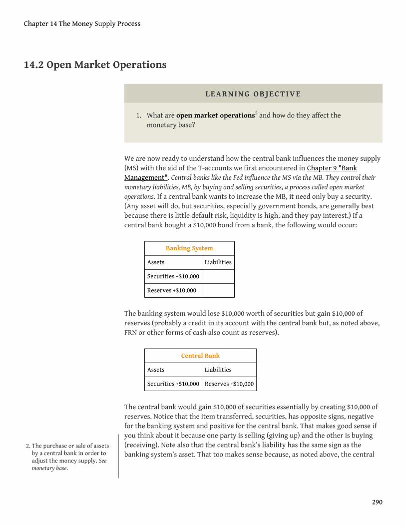
14.2 Open Market Operations
LEARNING OBJECTIVE
1. What are open market operations2 and how do they affect themonetary base?
We are now ready to understand how the central bank influences the money supply(MS) with the aid of the T-accounts we first encountered in Chapter 9 "BankManagement". Central banks like the Fed influence the MS via the MB. They control theirmonetary liabilities, MB, by buying and selling securities, a process called open marketoperations. If a central bank wants to increase the MB, it need only buy a security.(Any asset will do, but securities, especially government bonds, are generally bestbecause there is little default risk, liquidity is high, and they pay interest.) If acentral bank bought a $10,000 bond from a bank, the following would occur:
Banking System
Assets Liabilities
Securities −$10,000
Reserves +$10,000
The banking system would lose $10,000 worth of securities but gain $10,000 ofreserves (probably a credit in its account with the central bank but, as noted above,FRN or other forms of cash also count as reserves).
Central Bank
Assets Liabilities
Securities +$10,000 Reserves +$10,000
The central bank would gain $10,000 of securities essentially by creating $10,000 ofreserves. Notice that the item transferred, securities, has opposite signs, negativefor the banking system and positive for the central bank. That makes good sense ifyou think about it because one party is selling (giving up) and the other is buying(receiving). Note also that the central bank’s liability has the same sign as thebanking system’s asset. That too makes sense because, as noted above, the central
2. The purchase or sale of assetsby a central bank in order toadjust the money supply. Seemonetary base.
Chapter 14 The Money Supply Process
290
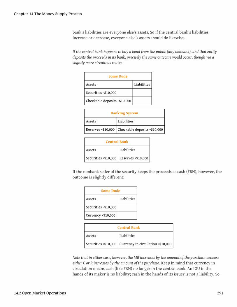
bank’s liabilities are everyone else’s assets. So if the central bank’s liabilitiesincrease or decrease, everyone else’s assets should do likewise.
If the central bank happens to buy a bond from the public (any nonbank), and that entitydeposits the proceeds in its bank, precisely the same outcome would occur, though via aslightly more circuitous route:
Some Dude
Assets Liabilities
Securities −$10,000
Checkable deposits +$10,000
Banking System
Assets Liabilities
Reserves +$10,000 Checkable deposits +$10,000
Central Bank
Assets Liabilities
Securities +$10,000 Reserves +$10,000
If the nonbank seller of the security keeps the proceeds as cash (FRN), however, theoutcome is slightly different:
Some Dude
Assets Liabilities
Securities −$10,000
Currency +$10,000
Central Bank
Assets Liabilities
Securities +$10,000 Currency in circulation +$10,000
Note that in either case, however, the MB increases by the amount of the purchase becauseeither C or R increases by the amount of the purchase. Keep in mind that currency incirculation means cash (like FRN) no longer in the central bank. An IOU in thehands of its maker is no liability; cash in the hands of its issuer is not a liability. So
Chapter 14 The Money Supply Process
14.2 Open Market Operations 291

although the money existed physically before Some Dude sold his bond, it did notexist economically as money until it left its papa (mama?), the central bank. If thetransaction were reversed and Some Dude bought a bond from the central bankwith currency, the notes he paid would cease to be money, and currency incirculation would decrease by $10,000.
In fact, whenever the central bank sells an asset, the exact opposite of the above T-accounts occurs: the MB shrinks because C (and/or R) decreases along with the centralbank’s securities holdings, and banks or the nonbank public own more securities but less C orR.
The nonbank public can influence the relative share of C and R but not the MB. Say thatyou had $55.50 in your bank account but wanted $30 in cash to take your significantother to the carnival. Your T-account would look like the following because youturned $30 of deposits into $30 of FRN:
Your T-Account
Assets Liabilities
Checkable deposits −$30.00
Currency +$30.00
Your bank’s T-account would look like the following because it lost $30 of depositsand $30 of reserves, the $30 you walked off with:
Your Bank
Assets Liabilities
Reserves −$30.00 Checkable deposits −$30.00
The central bank’s T-account would look like the following because the nonbankpublic (you!) would hold $30 and your bank’s reserves would decrease accordingly(as noted above):
Central Bank
Assets Liabilities
Currency in circulation $30.00
Reserves −$30.00
Chapter 14 The Money Supply Process
14.2 Open Market Operations 292
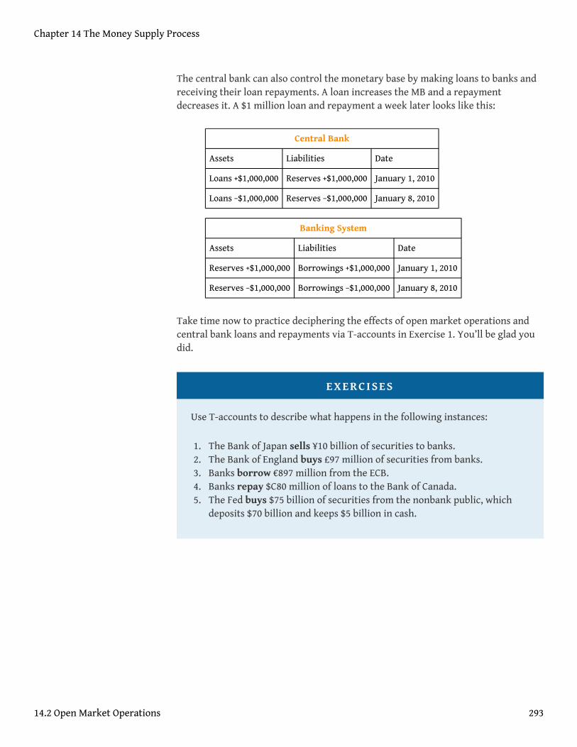
The central bank can also control the monetary base by making loans to banks andreceiving their loan repayments. A loan increases the MB and a repaymentdecreases it. A $1 million loan and repayment a week later looks like this:
Central Bank
Assets Liabilities Date
Loans +$1,000,000 Reserves +$1,000,000 January 1, 2010
Loans −$1,000,000 Reserves −$1,000,000 January 8, 2010
Banking System
Assets Liabilities Date
Reserves +$1,000,000 Borrowings +$1,000,000 January 1, 2010
Reserves −$1,000,000 Borrowings −$1,000,000 January 8, 2010
Take time now to practice deciphering the effects of open market operations andcentral bank loans and repayments via T-accounts in Exercise 1. You’ll be glad youdid.
EXERCISES
Use T-accounts to describe what happens in the following instances:
1. The Bank of Japan sells ¥10 billion of securities to banks.2. The Bank of England buys £97 million of securities from banks.3. Banks borrow €897 million from the ECB.4. Banks repay $C80 million of loans to the Bank of Canada.5. The Fed buys $75 billion of securities from the nonbank public, which
deposits $70 billion and keeps $5 billion in cash.
Chapter 14 The Money Supply Process
14.2 Open Market Operations 293
KEY TAKEAWAYS
• Open market operations occur whenever a central bank buys or sellsassets, usually government bonds.
• By purchasing bonds (or anything else for that matter), the central bankincreases the monetary base and hence, by some multiple, the moneysupply. (Picture the central bank giving up some money to acquire thebond, thereby putting FRN or reserves into circulation.)
• By selling bonds, the central bank decreases the monetary base andhence the money supply by some multiple. (Picture the central bankgiving up a bond and receiving money for it, removing FRN or reservesfrom circulation.)
• Similarly, the MB and MS increase whenever the Fed makes a loan, andthey decrease whenever a borrower repays the Fed.
Chapter 14 The Money Supply Process
14.2 Open Market Operations 294
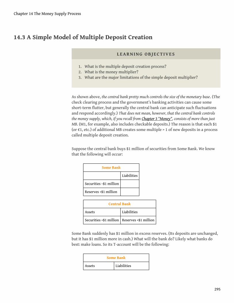
14.3 A Simple Model of Multiple Deposit Creation
LEARNING OBJECTIVES
1. What is the multiple deposit creation process?2. What is the money multiplier?3. What are the major limitations of the simple deposit multiplier?
As shown above, the central bank pretty much controls the size of the monetary base. (Thecheck clearing process and the government’s banking activities can cause someshort-term flutter, but generally the central bank can anticipate such fluctuationsand respond accordingly.) That does not mean, however, that the central bank controlsthe money supply, which, if you recall from Chapter 3 "Money", consists of more than justMB. (M1, for example, also includes checkable deposits.) The reason is that each $1(or €1, etc.) of additional MB creates some multiple > 1 of new deposits in a processcalled multiple deposit creation.
Suppose the central bank buys $1 million of securities from Some Bank. We knowthat the following will occur:
Some Bank
Liabilities
Securities −$1 million
Reserves +$1 million
Central Bank
Assets Liabilities
Securities +$1 million Reserves +$1 million
Some Bank suddenly has $1 million in excess reserves. (Its deposits are unchanged,but it has $1 million more in cash.) What will the bank do? Likely what banks dobest: make loans. So its T-account will be the following:
Some Bank
Assets Liabilities
Chapter 14 The Money Supply Process
295
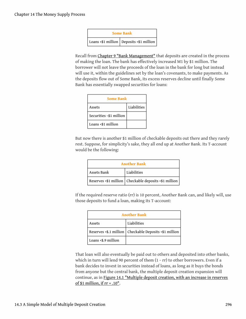
Some Bank
Loans +$1 million Deposits +$1 million
Recall from Chapter 9 "Bank Management" that deposits are created in the processof making the loan. The bank has effectively increased M1 by $1 million. Theborrower will not leave the proceeds of the loan in the bank for long but insteadwill use it, within the guidelines set by the loan’s covenants, to make payments. Asthe deposits flow out of Some Bank, its excess reserves decline until finally SomeBank has essentially swapped securities for loans:
Some Bank
Assets Liabilities
Securities −$1 million
Loans +$1 million
But now there is another $1 million of checkable deposits out there and they rarelyrest. Suppose, for simplicity’s sake, they all end up at Another Bank. Its T-accountwould be the following:
Another Bank
Assets Bank Liabilities
Reserves +$1 million Checkable deposits +$1 million
If the required reserve ratio (rr) is 10 percent, Another Bank can, and likely will, usethose deposits to fund a loan, making its T-account:
Another Bank
Assets Liabilities
Reserves +$.1 million Checkable Deposits +$1 million
Loans +$.9 million
That loan will also eventually be paid out to others and deposited into other banks,which in turn will lend 90 percent of them (1 − rr) to other borrowers. Even if abank decides to invest in securities instead of loans, as long as it buys the bondsfrom anyone but the central bank, the multiple deposit creation expansion willcontinue, as in Figure 14.1 "Multiple deposit creation, with an increase in reservesof $1 million, if rr = .10".
Chapter 14 The Money Supply Process
14.3 A Simple Model of Multiple Deposit Creation 296
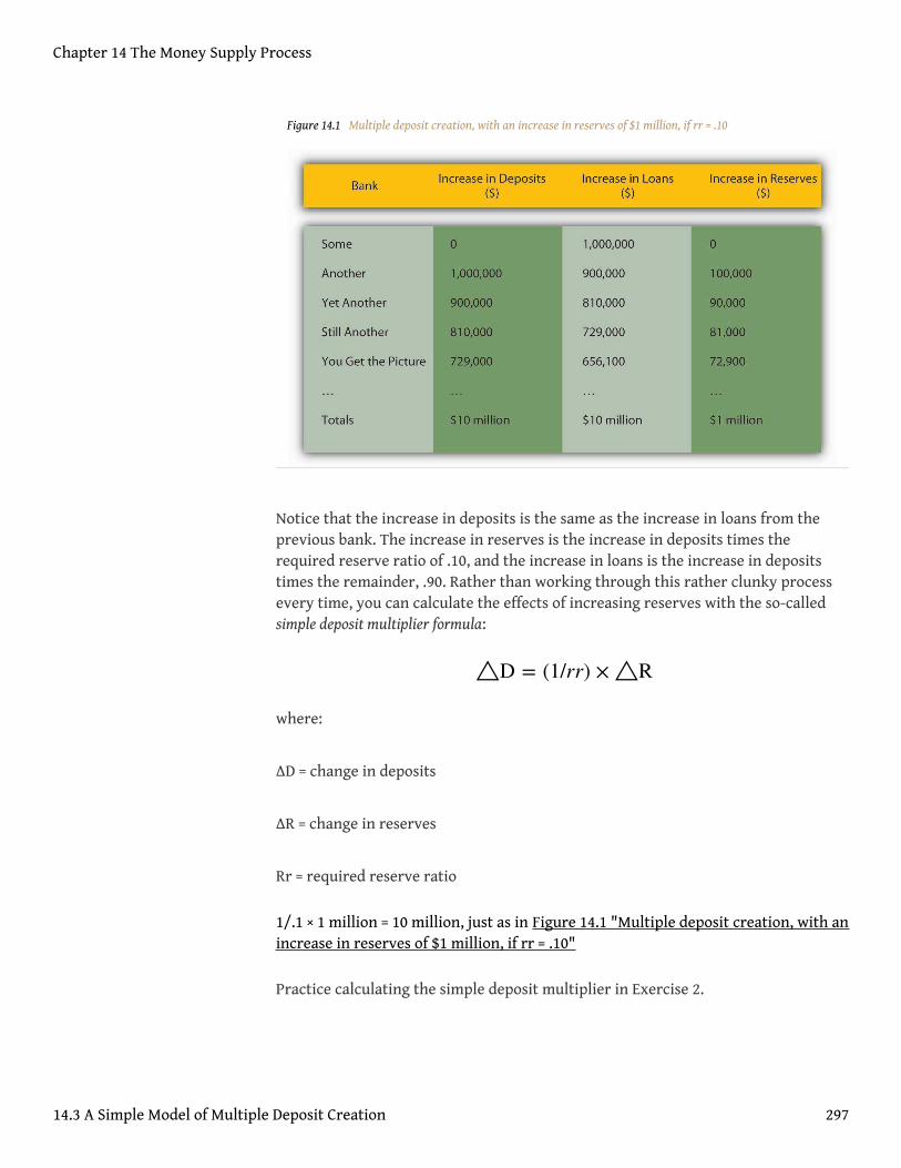
Figure 14.1 Multiple deposit creation, with an increase in reserves of $1 million, if rr = .10
Notice that the increase in deposits is the same as the increase in loans from theprevious bank. The increase in reserves is the increase in deposits times therequired reserve ratio of .10, and the increase in loans is the increase in depositstimes the remainder, .90. Rather than working through this rather clunky processevery time, you can calculate the effects of increasing reserves with the so-calledsimple deposit multiplier formula:
where:
∆D = change in deposits
∆R = change in reserves
Rr = required reserve ratio
1/.1 × 1 million = 10 million, just as in Figure 14.1 "Multiple deposit creation, with anincrease in reserves of $1 million, if rr = .10"
Practice calculating the simple deposit multiplier in Exercise 2.
△D = (1/rr) × △R
Chapter 14 The Money Supply Process
14.3 A Simple Model of Multiple Deposit Creation 297
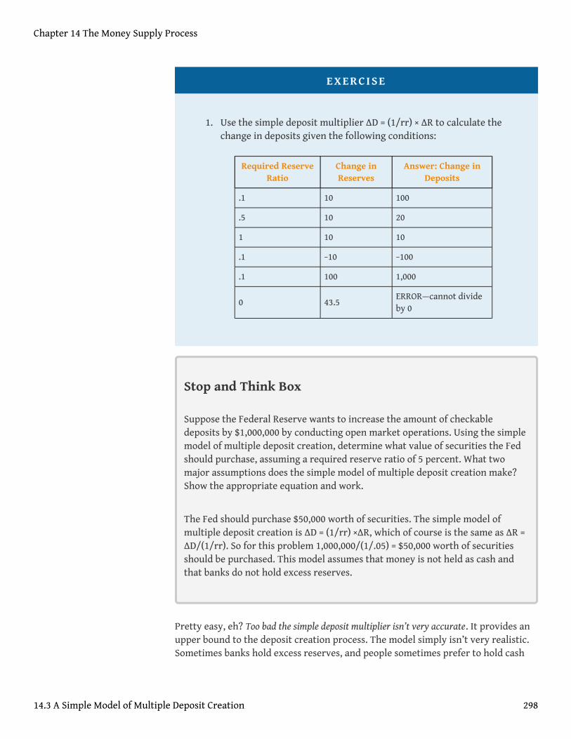
EXERCISE
1. Use the simple deposit multiplier ∆D = (1/rr) × ∆R to calculate thechange in deposits given the following conditions:
Required ReserveRatio
Change inReserves
Answer: Change inDeposits
.1 10 100
.5 10 20
1 10 10
.1 −10 −100
.1 100 1,000
0 43.5ERROR—cannot divideby 0
Stop and Think Box
Suppose the Federal Reserve wants to increase the amount of checkabledeposits by $1,000,000 by conducting open market operations. Using the simplemodel of multiple deposit creation, determine what value of securities the Fedshould purchase, assuming a required reserve ratio of 5 percent. What twomajor assumptions does the simple model of multiple deposit creation make?Show the appropriate equation and work.
The Fed should purchase $50,000 worth of securities. The simple model ofmultiple deposit creation is ∆D = (1/rr) ×∆R, which of course is the same as ∆R =∆D/(1/rr). So for this problem 1,000,000/(1/.05) = $50,000 worth of securitiesshould be purchased. This model assumes that money is not held as cash andthat banks do not hold excess reserves.
Pretty easy, eh? Too bad the simple deposit multiplier isn’t very accurate. It provides anupper bound to the deposit creation process. The model simply isn’t very realistic.Sometimes banks hold excess reserves, and people sometimes prefer to hold cash
Chapter 14 The Money Supply Process
14.3 A Simple Model of Multiple Deposit Creation 298

instead of deposits, thereby stopping the multiple deposit creation process cold.That is why, at the beginning of the chapter, we said that depositors, borrowers,and banks were also important players in the money supply determination process.In the next chapter, we’ll take their decisions into account.
KEY TAKEAWAYS
• The multiple deposit creation process works like this: say that thecentral bank buys $100 of securities from Bank 1, which lends the $100in cash it receives to some borrower. Said borrower writes checksagainst the $100 in deposits created by the loan until all the money restsin Bank 2. Its deposits and reserves increased by $100, Bank 2 lends asmuch as it can, say (1 – rr = .9) or $90, to another borrower, who writeschecks against it until it winds up in Bank 3, which also lends 90 percentof it. Bank 4 lends 90 percent of that, Bank 5 lends 90 percent of that,and so on, until a $100 initial increase in reserves has led to a $1,000increase in deposits (and loans).
• The simple deposit multiplier is ∆D = (1/rr) × ∆R, where ∆D = change indeposits; ∆R = change in reserves; rr = required reserve ratio.
• The simple deposit multiplier assumes that banks hold no excessreserves and that the public holds no currency. We all know whathappens when we assume or ass|u|me. These assumptions mean that thesimple deposit multiplier overestimates the multiple deposit creationprocess, providing us with an upper-bound estimate.
Chapter 14 The Money Supply Process
14.3 A Simple Model of Multiple Deposit Creation 299
14.4 Suggested Reading
Hummel, William. Money: What It Is, How It Works 2nd ed. Bloomington, IN: iUniverse,2006.
Mayes, David, and Jan Toporowski. Open Market Operations and Financial Markets. NewYork: Routledge, 2007.
Chapter 14 The Money Supply Process
300
Chapter 15
The Money Supply and the Money Multiplier
CHAPTER OBJECTIVES
By the end of this chapter, students should be able to:
1. Compare and contrast the simple money multiplier developed inChapter 14 "The Money Supply Process" and the m1 and m2 multipliersdeveloped in this chapter.
2. Write the equation that helps us to understand how changes in themonetary base affect the money supply.
3. Explain why the M2 multiplier is almost always larger than the m1
multiplier.4. Explain why the required reserve ratio, the excess reserve ratio, and the
currency ratio are in the denominator of the m1 and m2 moneymultipliers.
5. Explain why the currency, time deposit, and money market mutual fundratios are in the numerator of the M2 money multiplier.
6. Describe how central banks influence the money supply.7. Describe how banks, borrowers, and depositors influence the money
supply.
301
15.1 A More Sophisticated Money Multiplier for M1
LEARNING OBJECTIVES
1. How do the simple money multiplier and the more sophisticated onedeveloped here contrast and compare?
2. What equation helps us to understand how changes in the monetarybase affect the money supply?
In Chapter 14 "The Money Supply Process", you learned that an increase (decrease)in the monetary base (MB, which = C + R) leads to an even greater increase(decrease) in the money supply (MS, such as M11 or M22) due to the multipledeposit creation process. You also learned a simple but unrealistic upper-boundformula for estimating the change that assumed that banks hold no excess reservesand that the public holds no currency.
Stop and Think Box
You are a research associate for Moody’s subsidiary, High FrequencyEconomics, in West Chester, Pennsylvania. A client wants you to projectchanges in M1 given likely increases in the monetary base. Because of a glitchin the Federal Reserve’s computer systems, currency, deposit, and excessreserve figures will not be available for at least one week. A private firm,however, can provide you with good estimates of changes in banking systemreserves, and of course the required reserve ratio is well known. What equationcan you use to help your client? What are the equation’s assumptions andlimitations?
You cannot use the more complex M1 money multiplier this week because ofthe Fed’s computer glitch, so you should use the simple deposit multiplier fromChapter 14 "The Money Supply Process": ΔD = (1/rr) × ΔR. The equationprovides an upper-bound estimate for changes in deposits. It assumes that thepublic will hold no more currency and that banks will hold no increased excessreserves.
1. M1 is a measure of the moneysupply that includes currencyin circulation plus checkabledeposits.
2. M2 is a measure of the moneysupply that includes M1 plustime deposits andnoninstitutional (retail) moneymarket funds.
Chapter 15 The Money Supply and the Money Multiplier
302
To get a more realistic estimate, we’ll have to do a little more work. We start with theobservation that we can consider the money supply to be a function of the monetary basetimes some money multiplier (m):
This is basically a less specific version of the formula you learned in Chapter 14"The Money Supply Process", except that instead of calculating the change indeposits (ΔD) brought about by the change in reserves (ΔR), we will now calculatethe change in the money supply (ΔMS) brought about by the change in themonetary base (ΔMB). Furthermore, instead of using the reciprocal of the required reserveratio (1/rr) as the multiplier, we will use a more sophisticated one (m1, and later M2) that
doesn’t assume away cash and excess reserves.
We can add currency and excess reserves to the equation by algebraically describing theirrelationship to checkable deposits3in the form of a ratio:
C/D = currency ratio
ER/D = excess reserves ratio
Recall that required reserves are equal to checkable deposits (D) times the required reserveratio (rr). Total reserves equal required reserves plus excess reserves:
So we can render MB = C + R as MB = C + rrD + ER. Note that we have successfullyremoved C and ER from the multiple deposit expansion process by separating themfrom rrD. After further algebraic manipulations of the above equation and thereciprocal of the reserve ratio (1/rr) concept embedded in the simple depositmultiplier, we’re left with a more sophisticated, more realistic money multiplier:
So if
Required reserve ratio (rr) = .2
Currency in circulation = $100 billion
△MS = m × △MB
R = rrD + ER
m1 = 1 + (C/D)/[rr + (ER/D) + (C/D)]
3. Deposits that can easily,cheaply, and quickly be drawnupon by check in order tomake payments. Also known astransaction deposits.
Chapter 15 The Money Supply and the Money Multiplier
15.1 A More Sophisticated Money Multiplier for M1 303
Deposits = $400 billion
Excess reserves = $10 billion
Practice calculating the money multiplier in Exercise 1.
m1 = 1 + (100/400)/(.2 + (10/400) + (100/400))
m1 = 1.25/(.2 + .025 + .25)
m1 = 1.25/.475 = 2.6316
Chapter 15 The Money Supply and the Money Multiplier
15.1 A More Sophisticated Money Multiplier for M1 304
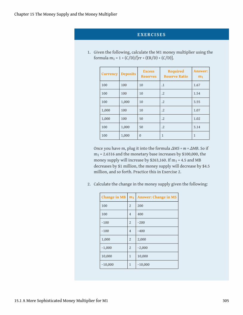
EXERCISES
1. Given the following, calculate the M1 money multiplier using theformula m1 = 1 + (C/D)/[rr + (ER/D) + (C/D)].
Currency DepositsExcess
ReservesRequired
Reserve RatioAnswer:
m1
100 100 10 .1 1.67
100 100 10 .2 1.54
100 1,000 10 .2 3.55
1,000 100 10 .2 1.07
1,000 100 50 .2 1.02
100 1,000 50 .2 3.14
100 1,000 0 1 1
Once you have m, plug it into the formula ΔMS = m × ΔMB. So ifm1 = 2.6316 and the monetary base increases by $100,000, themoney supply will increase by $263,160. If m1 = 4.5 and MBdecreases by $1 million, the money supply will decrease by $4.5million, and so forth. Practice this in Exercise 2.
2. Calculate the change in the money supply given the following:
Change in MB m1 Answer: Change in MS
100 2 200
100 4 400
−100 2 −200
−100 4 −400
1,000 2 2,000
−1,000 2 −2,000
10,000 1 10,000
−10,000 1 −10,000
Chapter 15 The Money Supply and the Money Multiplier
15.1 A More Sophisticated Money Multiplier for M1 305
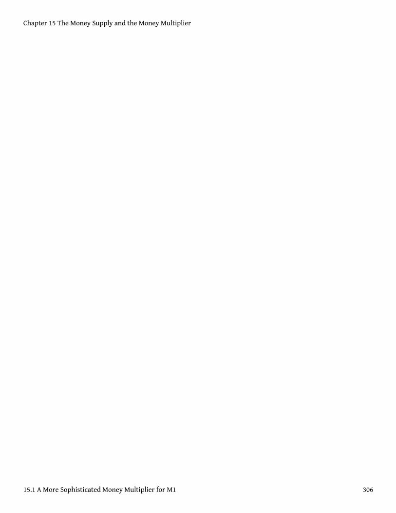
Chapter 15 The Money Supply and the Money Multiplier
15.1 A More Sophisticated Money Multiplier for M1 306
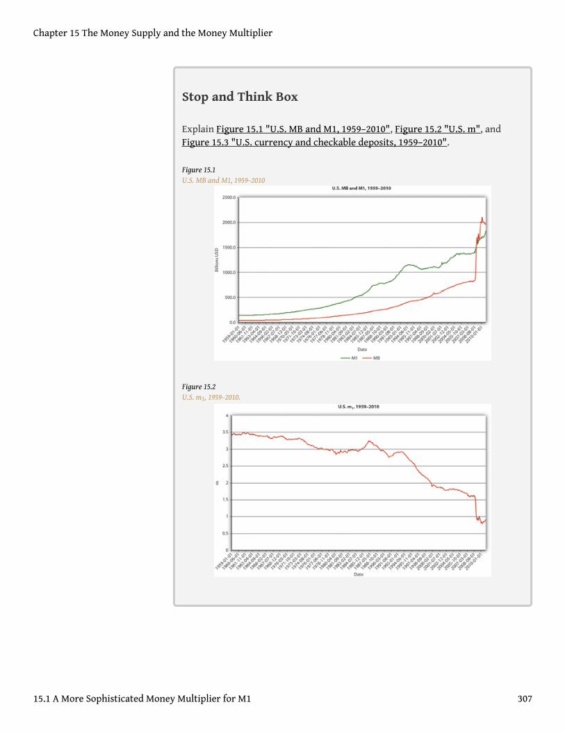
Stop and Think Box
Explain Figure 15.1 "U.S. MB and M1, 1959–2010", Figure 15.2 "U.S. m", andFigure 15.3 "U.S. currency and checkable deposits, 1959–2010".
Figure 15.1U.S. MB and M1, 1959–2010
Figure 15.2U.S. m1, 1959–2010.
Chapter 15 The Money Supply and the Money Multiplier
15.1 A More Sophisticated Money Multiplier for M1 307
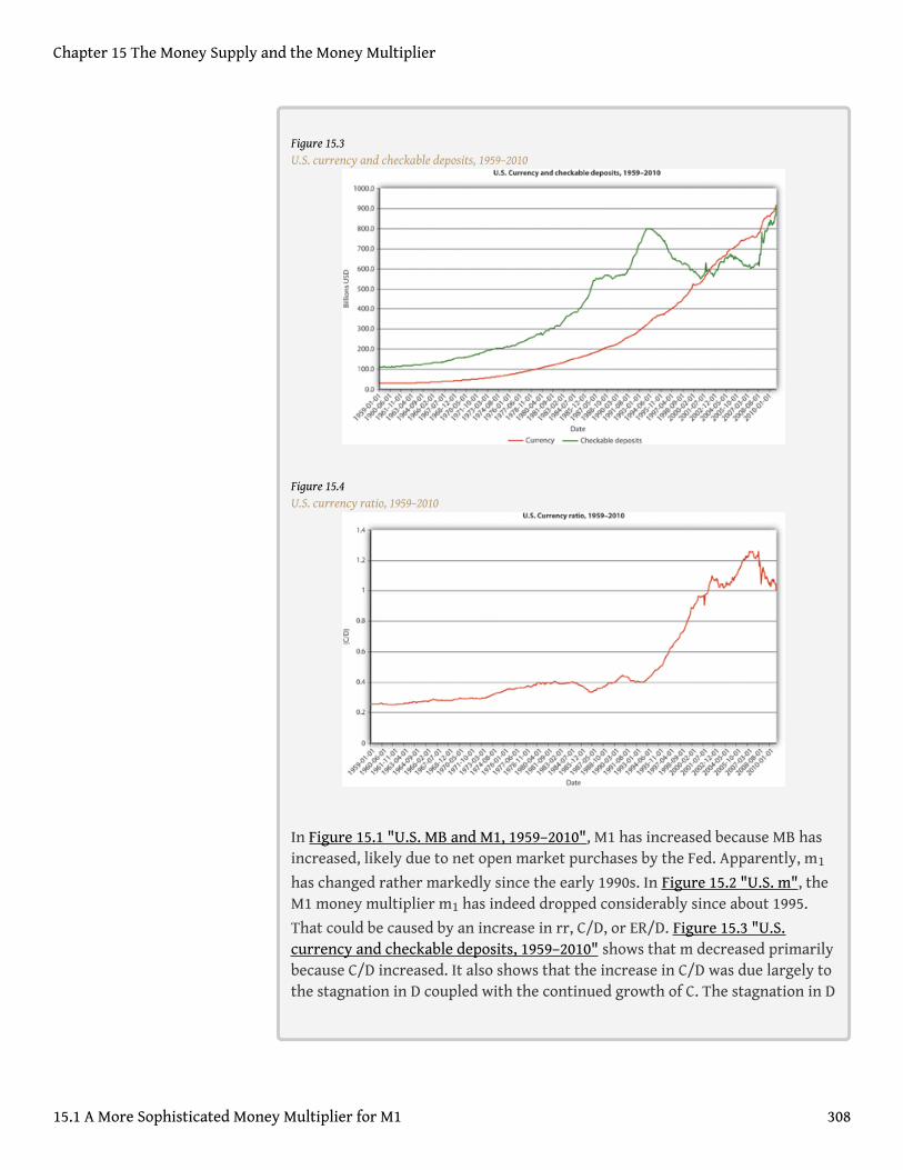
Figure 15.3U.S. currency and checkable deposits, 1959–2010
Figure 15.4U.S. currency ratio, 1959–2010
In Figure 15.1 "U.S. MB and M1, 1959–2010", M1 has increased because MB hasincreased, likely due to net open market purchases by the Fed. Apparently, m1
has changed rather markedly since the early 1990s. In Figure 15.2 "U.S. m", theM1 money multiplier m1 has indeed dropped considerably since about 1995.
That could be caused by an increase in rr, C/D, or ER/D. Figure 15.3 "U.S.currency and checkable deposits, 1959–2010" shows that m decreased primarilybecause C/D increased. It also shows that the increase in C/D was due largely tothe stagnation in D coupled with the continued growth of C. The stagnation in D
Chapter 15 The Money Supply and the Money Multiplier
15.1 A More Sophisticated Money Multiplier for M1 308
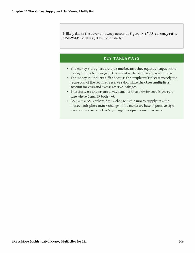
is likely due to the advent of sweep accounts. Figure 15.4 "U.S. currency ratio,1959–2010" isolates C/D for closer study.
KEY TAKEAWAYS
• The money multipliers are the same because they equate changes in themoney supply to changes in the monetary base times some multiplier.
• The money multipliers differ because the simple multiplier is merely thereciprocal of the required reserve ratio, while the other multipliersaccount for cash and excess reserve leakages.
• Therefore, m1 and m2 are always smaller than 1/rr (except in the rarecase where C and ER both = 0).
• ΔMS = m × ΔMB, where ΔMS = change in the money supply; m = themoney multiplier; ΔMB = change in the monetary base. A positive signmeans an increase in the MS; a negative sign means a decrease.
Chapter 15 The Money Supply and the Money Multiplier
15.1 A More Sophisticated Money Multiplier for M1 309
15.2 The M2 Money Multiplier
LEARNING OBJECTIVES
1. Why is the M2 multiplier almost always larger than the M1 multiplier?2. Why are the required reserve ratio, the excess reserve ratio, and the
currency ratio in the denominator of the m1 and m2 money multipliers?3. Why are the currency, time deposit, and money market mutual fund
ratios in the numerator of the m2 money multiplier?
Note that m1 is the M1 money multiplier. With a little bit more work, one can also calculate
the M2 money multiplier (m2). Recall from Chapter 3 "Money" that M2 = C + D + T +
MMF, where T = time and savings deposits and MMF = money market funds, moneymarket deposit accounts, and overnight loans. We account for the extra types ofdeposits in the same way as we accounted for currency and excess reserves, byexpressing them as ratios against checkable deposits:
(T/D) = time deposit ratio
(MMF/D) = money market ratio
which leads to the following equation:
Once you calculate M2, multiply it by the change in MB to calculate the change inthe MS, specifically in M2, just as you did in Exercise 2. Notice that the denominatorof the m2 equation is the same as the m1 equation but that we have added the time
and money market ratios to the numerator. So M2 is alwaysM2 would equal m1 iff T =
0 and MMF = 0, which is highly unlikely. Note: iff means if and only if. > m1, ceteris
paribus, which makes sense when you recall that M2 is composed of M1 plus other forms ofmoney. To verify this, recall that we calculated m1 as 2.6316 when
Required reserves (rr) = .2
Currency in circulation = $100 million
m2 = 1 + (C/D) + (T/D) + (MMF/D)/[rr + (ER/D) + (C/D)]
Chapter 15 The Money Supply and the Money Multiplier
310
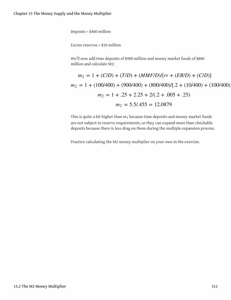
Deposits = $400 million
Excess reserves = $10 million
We’ll now add time deposits of $900 million and money market funds of $800million and calculate M2:
This is quite a bit higher than m1 because time deposits and money market funds
are not subject to reserve requirements, so they can expand more than checkabledeposits because there is less drag on them during the multiple expansion process.
Practice calculating the M2 money multiplier on your own in the exercise.
m2 = 1 + (C/D) + (T/D) + (MMF/D)/[rr + (ER/D) + (C/D)]
m2 = 1 + (100/400) + (900/400) + (800/400)/[.2 + (10/400) + (100/400)]
m2 = 1 + .25 + 2.25 + 2/(.2 + .005 + .25)
m2 = 5.5/.455 = 12.0879
Chapter 15 The Money Supply and the Money Multiplier
15.2 The M2 Money Multiplier 311
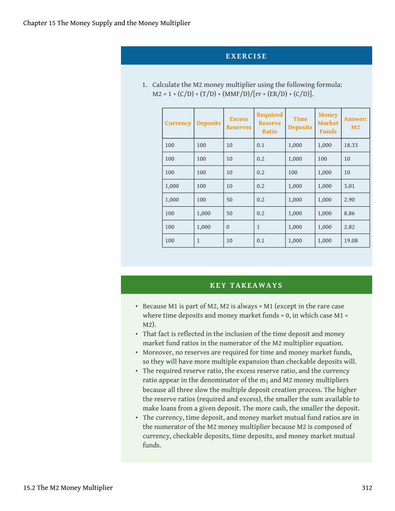
EXERCISE
1. Calculate the M2 money multiplier using the following formula:M2 = 1 + (C/D) + (T/D) + (MMF/D)/[rr + (ER/D) + (C/D)].
Currency DepositsExcess
Reserves
RequiredReserve
Ratio
TimeDeposits
MoneyMarketFunds
Answer:M2
100 100 10 0.1 1,000 1,000 18.33
100 100 10 0.2 1,000 100 10
100 100 10 0.2 100 1,000 10
1,000 100 10 0.2 1,000 1,000 3.01
1,000 100 50 0.2 1,000 1,000 2.90
100 1,000 50 0.2 1,000 1,000 8.86
100 1,000 0 1 1,000 1,000 2.82
100 1 10 0.1 1,000 1,000 19.08
KEY TAKEAWAYS
• Because M1 is part of M2, M2 is always > M1 (except in the rare casewhere time deposits and money market funds = 0, in which case M1 =M2).
• That fact is reflected in the inclusion of the time deposit and moneymarket fund ratios in the numerator of the M2 multiplier equation.
• Moreover, no reserves are required for time and money market funds,so they will have more multiple expansion than checkable deposits will.
• The required reserve ratio, the excess reserve ratio, and the currencyratio appear in the denominator of the m1 and M2 money multipliersbecause all three slow the multiple deposit creation process. The higherthe reserve ratios (required and excess), the smaller the sum available tomake loans from a given deposit. The more cash, the smaller the deposit.
• The currency, time deposit, and money market mutual fund ratios are inthe numerator of the M2 money multiplier because M2 is composed ofcurrency, checkable deposits, time deposits, and money market mutualfunds.
Chapter 15 The Money Supply and the Money Multiplier
15.2 The M2 Money Multiplier 312
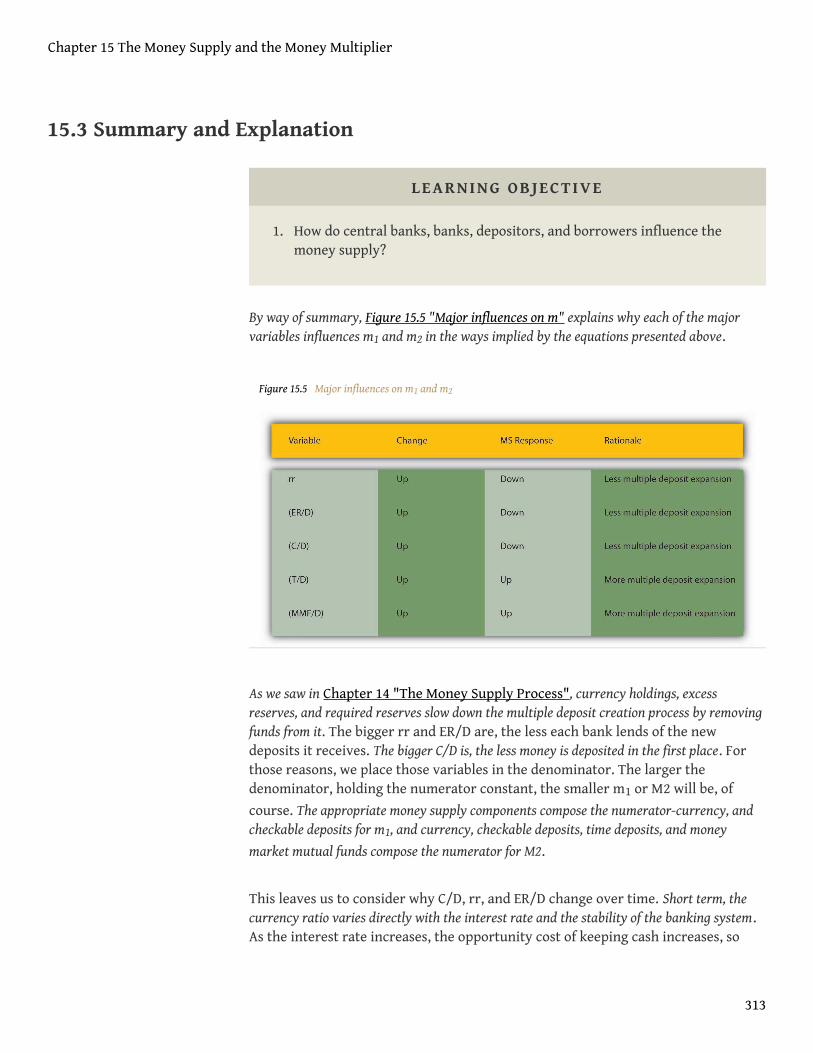
15.3 Summary and Explanation
LEARNING OBJECTIVE
1. How do central banks, banks, depositors, and borrowers influence themoney supply?
By way of summary, Figure 15.5 "Major influences on m" explains why each of the majorvariables influences m1 and m2 in the ways implied by the equations presented above.
Figure 15.5 Major influences on m1 and m2
As we saw in Chapter 14 "The Money Supply Process", currency holdings, excessreserves, and required reserves slow down the multiple deposit creation process by removingfunds from it. The bigger rr and ER/D are, the less each bank lends of the newdeposits it receives. The bigger C/D is, the less money is deposited in the first place. Forthose reasons, we place those variables in the denominator. The larger thedenominator, holding the numerator constant, the smaller m1 or M2 will be, of
course. The appropriate money supply components compose the numerator-currency, andcheckable deposits for m1, and currency, checkable deposits, time deposits, and money
market mutual funds compose the numerator for M2.
This leaves us to consider why C/D, rr, and ER/D change over time. Short term, thecurrency ratio varies directly with the interest rate and the stability of the banking system.As the interest rate increases, the opportunity cost of keeping cash increases, so
Chapter 15 The Money Supply and the Money Multiplier
313
people are less anxious to hold it. People are also less anxious to hold currency ifthe banking system is stable because their money is safer in a checking deposit. Ifinterest rates are extremely low or people believe the banks might be shaky, theynaturally want to hold more physical cash. Longer term, C/D may be influenced bytechnology and loophole mining, encouraging bankers and depositors to eschew traditionalcheckable deposits in favor of sweep accounts.
The required reserve ratio is mandated by the central bank but, as noted in Chapter10 "Innovation and Structure in Banking and Finance", loophole mining andtechnology have rendered it less important in recent years because sweep accountsallow banks to minimize the de jure level of their checkable deposits. In many places,rr is no longer a binding constraint on banks so, as we’ll see, most central banks no longerconsider changing it as an effective monetary policy tool. (This in no way affects themoney multiplier, which would provide the same figure for m1 or M2 whether we
calculate them as above or replace rr and ER/D with R/D, where R = total reserves.)
Stop and Think Box
Prove the assertion made above: “This in no way affects the money multiplier,which would provide the same figure for m1 or M2 whether we calculate them
as above or replace rr and ER/D with R/D, where R = total reserves.” Supposethat C = 100, R = 200, and D = 500 and that R is composed of required reserves of100 and excess reserves of 100. That means that rr must equal .2(100/500).
Under the formula provided in the text,
Under the formula suggested above,
Excess reserves (or just reserves in a system without required reserves) are inversely relatedto the interest rate. In the early 1960s and early 2000s, when the interest rate was wellless than 5 percent, ER/D was high, at .003 to .004. In the 1970s and 1980s, when
m1 = 1 + (C/D)/[rr + (ER/D) + (C/D)]
m1 = 1 + .2/.2 + .2 + .2 = 1.2/.6 = 2.0
m1 = 1 + (C/D)/[(R/D) + (C/D)]
m1 = 1.2/.4 + 2 = 2.0
Chapter 15 The Money Supply and the Money Multiplier
15.3 Summary and Explanation 314
interest rates were 10 percent and higher, ER/D dropped to .001 to .002. As welearned in Chapter 9 "Bank Management", expected deposit outflows directly affectexcess reserve levels as banks stock up on reserves to meet the outflows. When uncertaintyis high or a banking crisis is in progress or appears imminent, bankers will increaseER to protect their banks.
In summary, the central bank influences the money supply by controlling themonetary base and, to a far lesser extent, the required reserve ratio. Depositors,banks, and borrowers influence the money supply by influencing m1 and M2,
specifically by determining the money multiplier, with depositors largely in controlof C/D; depositors and banks interacting via deposit outflow expectations todetermine E/R; and borrowers, depositors, banks, and the central bank interactingto determine interest rates and hence to some extent both C/D and E/R.
KEY TAKEAWAYS
• Central banks control MB and rr, and affect interest rates, which in turnaffect C/D and ER/D.
• Depositors determine C/D by deciding how much cash versus deposits tohold. They also influence interest rates.
• Banks influence interest rates and determine ER/D by deciding howmany excess reserves to hold in the face of expected deposit outflowsand interest rates.
• Borrowers influence the interest rate and hence to some extent C/D andER/D.
Chapter 15 The Money Supply and the Money Multiplier
15.3 Summary and Explanation 315
15.4 Suggested Reading
Macesich, George. The Money Supply Process: A Comparative Analysis. New York:Praeger, 1999.
Chapter 15 The Money Supply and the Money Multiplier
316
Chapter 16
Monetary Policy Tools
CHAPTER OBJECTIVES
By the end of this chapter, students should be able to:
1. List and assess the strengths and weaknesses of the three primarymonetary policy tools that central banks have at their disposal.
2. Describe the federal funds market and explain its importance.3. Explain how the Fed influences the equilibrium fed funds rate to move
toward its target rate.4. Explain the purpose of the Fed’s discount window and other lending
facilities.5. Compare and contrast the monetary policy tools of central banks
worldwide to those of the Fed.
317
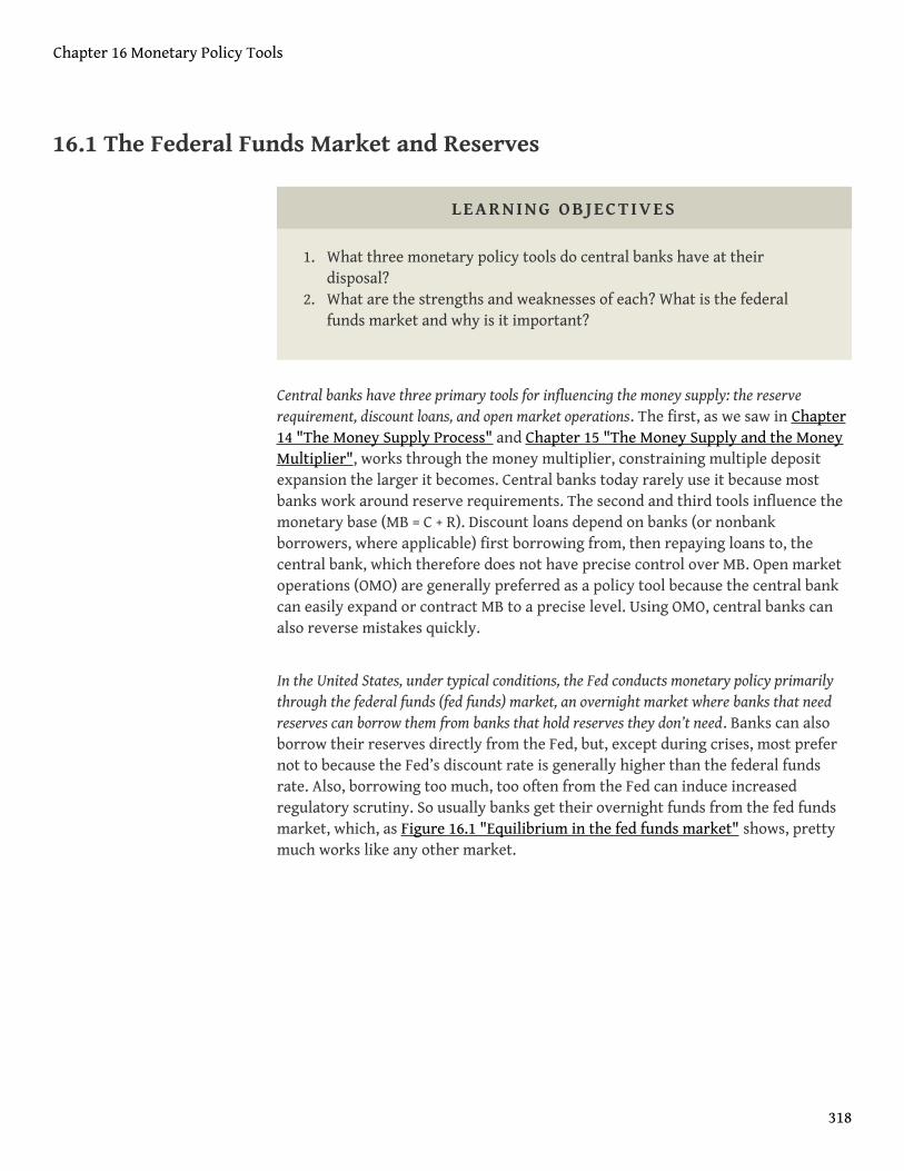
16.1 The Federal Funds Market and Reserves
LEARNING OBJECTIVES
1. What three monetary policy tools do central banks have at theirdisposal?
2. What are the strengths and weaknesses of each? What is the federalfunds market and why is it important?
Central banks have three primary tools for influencing the money supply: the reserverequirement, discount loans, and open market operations. The first, as we saw in Chapter14 "The Money Supply Process" and Chapter 15 "The Money Supply and the MoneyMultiplier", works through the money multiplier, constraining multiple depositexpansion the larger it becomes. Central banks today rarely use it because mostbanks work around reserve requirements. The second and third tools influence themonetary base (MB = C + R). Discount loans depend on banks (or nonbankborrowers, where applicable) first borrowing from, then repaying loans to, thecentral bank, which therefore does not have precise control over MB. Open marketoperations (OMO) are generally preferred as a policy tool because the central bankcan easily expand or contract MB to a precise level. Using OMO, central banks canalso reverse mistakes quickly.
In the United States, under typical conditions, the Fed conducts monetary policy primarilythrough the federal funds (fed funds) market, an overnight market where banks that needreserves can borrow them from banks that hold reserves they don’t need. Banks can alsoborrow their reserves directly from the Fed, but, except during crises, most prefernot to because the Fed’s discount rate is generally higher than the federal fundsrate. Also, borrowing too much, too often from the Fed can induce increasedregulatory scrutiny. So usually banks get their overnight funds from the fed fundsmarket, which, as Figure 16.1 "Equilibrium in the fed funds market" shows, prettymuch works like any other market.
Chapter 16 Monetary Policy Tools
318
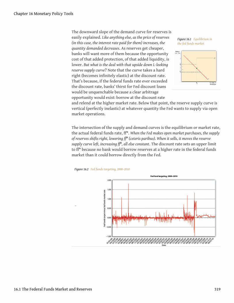
Figure 16.1 Equilibrium inthe fed funds market
The downward slope of the demand curve for reserves iseasily explained. Like anything else, as the price of reserves(in this case, the interest rate paid for them) increases, thequantity demanded decreases. As reserves get cheaper,banks will want more of them because the opportunitycost of that added protection, of that added liquidity, islower. But what is the deal with that upside down L-lookingreserve supply curve? Note that the curve takes a hardright (becomes infinitely elastic) at the discount rate.That’s because, if the federal funds rate ever exceededthe discount rate, banks’ thirst for Fed discount loanswould be unquenchable because a clear arbitrageopportunity would exist: borrow at the discount rateand relend at the higher market rate. Below that point, the reserve supply curve isvertical (perfectly inelastic) at whatever quantity the Fed wants to supply via openmarket operations.
The intersection of the supply and demand curves is the equilibrium or market rate,the actual federal funds rate, ff*. When the Fed makes open market purchases, the supplyof reserves shifts right, lowering ff* (ceteris paribus). When it sells, it moves the reservesupply curve left, increasing ff*, all else constant. The discount rate sets an upper limitto ff* because no bank would borrow reserves at a higher rate in the federal fundsmarket than it could borrow directly from the Fed.
Figure 16.2 Fed funds targeting, 2000–2010
Chapter 16 Monetary Policy Tools
16.1 The Federal Funds Market and Reserves 319
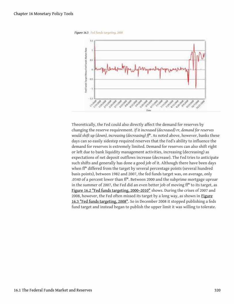
Figure 16.3 Fed funds targeting, 2008
Theoretically, the Fed could also directly affect the demand for reserves bychanging the reserve requirement. If it increased (decreased) rr, demand for reserveswould shift up (down), increasing (decreasing) ff*. As noted above, however, banks thesedays can so easily sidestep required reserves that the Fed’s ability to influence thedemand for reserves is extremely limited. Demand for reserves can also shift rightor left due to bank liquidity management activities, increasing (decreasing) asexpectations of net deposit outflows increase (decrease). The Fed tries to anticipatesuch shifts and generally has done a good job of it. Although there have been dayswhen ff* differed from the target by several percentage points (several hundredbasis points), between 1982 and 2007, the fed funds target was, on average, only.0340 of a percent lower than ff*. Between 2000 and the subprime mortgage uproarin the summer of 2007, the Fed did an even better job of moving ff* to its target, asFigure 16.2 "Fed funds targeting, 2000–2010" shows. During the crises of 2007 and2008, however, the Fed often missed its target by a long way, as shown in Figure16.3 "Fed funds targeting, 2008". So in December 2008 it stopped publishing a fedsfund target and instead began to publish the upper limit it was willing to tolerate.
Chapter 16 Monetary Policy Tools
16.1 The Federal Funds Market and Reserves 320
Stop and Think Box
In Chapter 13 "Central Bank Form and Function", you learned that America’sfirst central banks, the BUS and SBUS, controlled commercial bank reservelevels by varying the speed and intensity by which it redeemed convertiblebank liabilities (notes and deposits) for reserves (gold and silver). Can youmodel that system?
Kudos if you can! I’d plot quantity of reserves along the horizontal axis andinterest rate along the vertical axis. The reserve supply curve was probablyhighly but not perfectly inelastic and the reserve demand curve slopeddownward, of course. When the BUS or SBUS wanted to tighten monetarypolicy, it would return commercial bank monetary liabilities in a great rush,pushing the reserve demand curve to the right, thereby raising the interestrate. When it wanted to soften, it would dawdle before redeeming notes forgold and so forth, allowing the demand for reserves to move left, therebydecreasing the interest rate.
Chapter 16 Monetary Policy Tools
16.1 The Federal Funds Market and Reserves 321
KEY TAKEAWAYS
• Central banks can influence the money multiplier (simple, m1, m2, etc.)via reserve requirements.
• That tool is somewhat limited these days given the introduction ofsweep accounts and other reserve requirement loopholes.
• Central banks can also influence MB via loans to banks and open marketoperations.
• For day-to-day policy implementation, open market operations arepreferable because they are more precise and immediate and almostcompletely under the control of the central bank, which means it canreverse mistakes quickly.
• Discount loans depend on banks borrowing and repaying loans, so thecentral bank has less control over MB if it relies on loans alone.
• Discount loans are therefore used now primarily to set a ceiling on theovernight interbank rate and to provide liquidity during crises.
• The federal funds market is the name of the overnight interbank lendingmarket, basically the market where banks borrow and lend bankreserves, in the United States.
• It is important because the Fed uses open market operations (OMO) tomove the equilibrium rate ff* toward the target established by theFederal Open Market Committee (FOMC).
Chapter 16 Monetary Policy Tools
16.1 The Federal Funds Market and Reserves 322
16.2 Open Market Operations and the Discount Window
LEARNING OBJECTIVES
1. How does the Fed influence the equilibrium fed funds rate to movetoward its target rate?
2. What purpose does the Fed’s discount window now serve?
In practical terms, the Fed engages in two types of OMO, dynamic and defensive. As thosenames imply, it uses dynamic OMO to change the level of the MB, and defensiveOMO to offset movements in other factors affecting MB, with an eye towardmaintaining the federal funds target rate determined by the Federal Open MarketCommittee (FOMC) at its most recent meeting.
As noted in Chapter 13 "Central Bank Form and Function", the responsibility for actualbuying and selling government bonds devolves upon the Federal Reserve Bank of New York(FRBNY). Each trading day, FRBNY staff members look at the level of reserves, thefed funds target, the actual market fed funds rate, expectations regarding float, andTreasury activities. They also garner information about Treasury market conditionsthrough conversations with so-called primary dealers, specialized firms and banksthat make a market1 in Treasuries. With the input and consent of the MonetaryAffairs Division of the Board of Governors, the FRBNY determines how much to buyor sell and places the appropriate order on the Trading Room AutomatedProcessing System (TRAPS) computer system that links all the primary dealers. TheFRBNY then selects the best offers up to the amount it wants to buy or sell. It entersinto two types of trades, so-called outright ones, where the bonds permanently joinor leave the Fed’s balance sheet, and temporary ones, called repos and reverserepos. In a repo (aka a repurchase agreement), the Fed purchases governmentbonds with the guarantee that the sellers will repurchase them from the Fed,generally one to fifteen days hence. In a reverse repo (aka a matched sale-purchasetransaction), the Fed sells securities and the buyer agrees to sell them to the Fedagain in the near future. The availability of such self-reversing contracts and theliquidity of the government bond market render open market operations a precisetool for implementing the Fed’s monetary policy.
The so-called discount window, where banks come to borrow reserves from the Federaldistrict banks, is today primarily a backup facility used during crises, when the federal fundsmarket might not function effectively. As noted above, the discount rate puts aneffective cap on ff* by providing banks with an alternative source of reserves (see
1. Buying securities from allcomers at a bid price andreselling them to all comers ata slightly higher ask price.
Chapter 16 Monetary Policy Tools
323
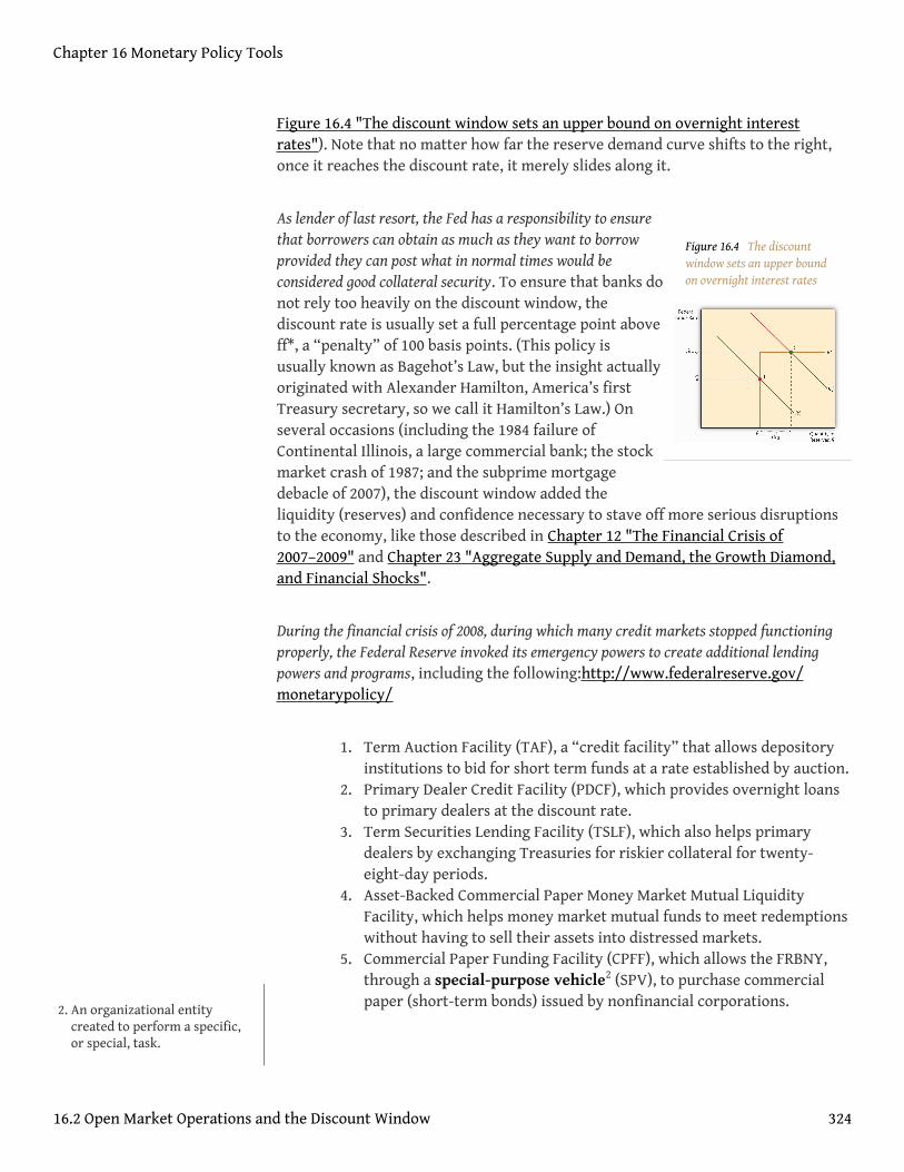
Figure 16.4 The discountwindow sets an upper boundon overnight interest rates
Figure 16.4 "The discount window sets an upper bound on overnight interestrates"). Note that no matter how far the reserve demand curve shifts to the right,once it reaches the discount rate, it merely slides along it.
As lender of last resort, the Fed has a responsibility to ensurethat borrowers can obtain as much as they want to borrowprovided they can post what in normal times would beconsidered good collateral security. To ensure that banks donot rely too heavily on the discount window, thediscount rate is usually set a full percentage point aboveff*, a “penalty” of 100 basis points. (This policy isusually known as Bagehot’s Law, but the insight actuallyoriginated with Alexander Hamilton, America’s firstTreasury secretary, so we call it Hamilton’s Law.) Onseveral occasions (including the 1984 failure ofContinental Illinois, a large commercial bank; the stockmarket crash of 1987; and the subprime mortgagedebacle of 2007), the discount window added theliquidity (reserves) and confidence necessary to stave off more serious disruptionsto the economy, like those described in Chapter 12 "The Financial Crisis of2007–2009" and Chapter 23 "Aggregate Supply and Demand, the Growth Diamond,and Financial Shocks".
During the financial crisis of 2008, during which many credit markets stopped functioningproperly, the Federal Reserve invoked its emergency powers to create additional lendingpowers and programs, including the following:http://www.federalreserve.gov/monetarypolicy/
1. Term Auction Facility (TAF), a “credit facility” that allows depositoryinstitutions to bid for short term funds at a rate established by auction.
2. Primary Dealer Credit Facility (PDCF), which provides overnight loansto primary dealers at the discount rate.
3. Term Securities Lending Facility (TSLF), which also helps primarydealers by exchanging Treasuries for riskier collateral for twenty-eight-day periods.
4. Asset-Backed Commercial Paper Money Market Mutual LiquidityFacility, which helps money market mutual funds to meet redemptionswithout having to sell their assets into distressed markets.
5. Commercial Paper Funding Facility (CPFF), which allows the FRBNY,through a special-purpose vehicle2 (SPV), to purchase commercialpaper (short-term bonds) issued by nonfinancial corporations.2. An organizational entity
created to perform a specific,or special, task.
Chapter 16 Monetary Policy Tools
16.2 Open Market Operations and the Discount Window 324
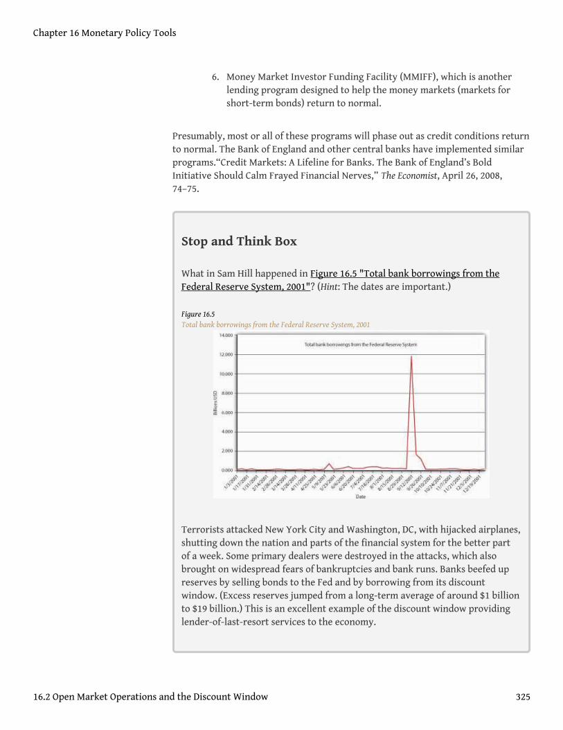
6. Money Market Investor Funding Facility (MMIFF), which is anotherlending program designed to help the money markets (markets forshort-term bonds) return to normal.
Presumably, most or all of these programs will phase out as credit conditions returnto normal. The Bank of England and other central banks have implemented similarprograms.“Credit Markets: A Lifeline for Banks. The Bank of England’s BoldInitiative Should Calm Frayed Financial Nerves,” The Economist, April 26, 2008,74–75.
Stop and Think Box
What in Sam Hill happened in Figure 16.5 "Total bank borrowings from theFederal Reserve System, 2001"? (Hint: The dates are important.)
Figure 16.5Total bank borrowings from the Federal Reserve System, 2001
Terrorists attacked New York City and Washington, DC, with hijacked airplanes,shutting down the nation and parts of the financial system for the better partof a week. Some primary dealers were destroyed in the attacks, which alsobrought on widespread fears of bankruptcies and bank runs. Banks beefed upreserves by selling bonds to the Fed and by borrowing from its discountwindow. (Excess reserves jumped from a long-term average of around $1 billionto $19 billion.) This is an excellent example of the discount window providinglender-of-last-resort services to the economy.
Chapter 16 Monetary Policy Tools
16.2 Open Market Operations and the Discount Window 325

The discount window is also used to provide moderately shaky banks a longer-term source ofcredit at an even higher penalty rate .5 percentage (50 basis) points above the regulardiscount rate. Finally, the Fed will also lend to a small number of banks in vacationand agricultural areas that experience large deposit fluctuations over the course ofa year. Increasingly, however, such banks are becoming part of larger banks withmore stable deposit profiles, or they handle their liquidity management using themarket for negotiable certificates of deposit NCDs or other market borrowings.
KEY TAKEAWAYS
• The Fed can move the equilibrium fed funds rate toward its target bychanging the demand for reserves by changing the required reserveratio. However, it rarely does so anymore.
• It can also shift the supply curve to the right (add reserves to thesystem) by buying assets (almost always Treasury bonds) or shift it tothe left (remove reserves from the system) by selling assets.
• The discount window caps ff* because if ff* were to rise above the Fed’sdiscount rate, banks would borrow reserves from the Fed (technically itsdistrict banks) instead of borrowing them from other banks in the fedfunds market.
• Because the Fed typically sets the discount rate a full percentage point(100 basis) points above its feds fund target, ff* rises above the discountrate only in a crisis, as in the aftermath of the 1987 stock market crashand the 2007 subprime mortgage debacle.
Chapter 16 Monetary Policy Tools
16.2 Open Market Operations and the Discount Window 326
16.3 The Monetary Policy Tools of Other Central Banks
LEARNING OBJECTIVE
1. In what ways are the monetary policy tools of central banks worldwidesimilar to those of the Fed? In what ways do they differ?
The European Central Bank (ECB) also uses open market operations to move the market forovernight interbank lending toward its target. It too uses repos and reverse repos forreversible, defensive OMO and outright purchases for permanent additions to MB.Unlike the Fed, however, the ECB spreads the love around, conducting OMO inmultiple cities throughout the European Union. The ECB’s national central banks(NCBs,) like the Fed’s district banks, also lend to banks at a so-called marginallending rate, which is generally set 100 basis points above the overnight cash rate.The ECB pays interest on reserves, a practice the Fed took up only recently.
Canada, New Zealand, and Australia do likewise and have eliminated reserverequirements, relying instead on what is called the channel, or corridor, system. AsFigure 16.6 "Paying interest on reserves puts a floor under the overnight interestrate" depicts, the supply curve in the corridor system looks like a backward Z. Thevertical part of the supply curve represents the area in which the central bankengages in OMO to influence the market rate, i*, to meet its target rate, it. The tophorizontal part of the supply curve, il for the Lombard rate, is the functionalequivalent of the discount rate in the American system. The ECB and other centralbanks using this system, like the Fed, will lend at this rate whatever amount bankswith good collateral desire to borrow. Under normal circumstances, that quantity isnil because it (and i*) will be 25, 50, or more basis points lower, depending on thecountry. The innovation is the lower horizontal part of the supply curve, ir, or the rate atwhich the central bank pays banks to hold reserves. That sets a floor on i* because nobank would lend in the overnight market if it could earn a higher return bydepositing its excess funds with the central bank. Using the corridor system, acentral bank can keep the overnight rate within the bands set by il and ir and useOMO to keep i* near it.
Chapter 16 Monetary Policy Tools
327

Figure 16.6 Paying interest on reserves puts a floor under the overnight interest rate
In response to the financial crisis of 2008, the Fed began to pay interest rates onreserves and will likely continue to do so because it appears to have become centralbank best practice3.
KEY TAKEAWAYS
• Most central banks now use OMO instead of discount loans or reserverequirement adjustments for conducting day-to-day monetary policy.
• Some central banks, including those of the euro zone and the BritishCommonwealth (Canada, Australia, and New Zealand) have developed aningenious new method called the channel or corridor system.
• Under that system, the central bank conducts OMO to get the overnightinterbank lending rate near the central bank’s target, as the Fed does inthe United States.
• That market rate is capped at both ends, however: on the upper end bythe discount (aka Lombard) rate, and at the lower end by the reserverate, the interest rate the central bank pays to banks for holdingreserves.
• The market overnight rate can never dip below that rate because bankswould simply invest their extra funds in the central bank rather thanlend them to other banks at a lower rate.
• During the financial crisis of 2008, the Fed adopted the corridor systemby paying interest on reserves.
3. Policies generally consideredto be state of the art in a givenindustry, to be something thatnonconforming organizationsought to emulate.
Chapter 16 Monetary Policy Tools
16.3 The Monetary Policy Tools of Other Central Banks 328
16.4 Suggested Reading
Axilrod, Stephen H. Inside the Fed: Monetary Policy and Its Management, Martin ThroughGreenspan to Bernanke. Cambridge, MA: MIT Press, 2009.
Hetzel, Robert L. The Monetary Policy of the Federal Reserve: A History. New York:Cambridge University Press, 2008.
Mishkin, Frederic S. Monetary Policy Strategy. Cambridge, MA: MIT Press, 2007.
Chapter 16 Monetary Policy Tools
329
Chapter 17
Monetary Policy Targets and Goals
CHAPTER OBJECTIVES
By the end of this chapter, students should be able to:
1. Explain why the Fed was generally so ineffective before the late 1980s.2. Explain why macroeconomic volatility declined from the late 1980s until
2008.3. List the trade-offs that central banks face and describe how they
confront them.4. Define monetary targeting and explain why it succeeded in some
countries and failed in others.5. Define inflation targeting and explain its importance.6. Provide and use the Taylor Rule and explain its importance.
330
17.1 A Short History of Fed Blunders
LEARNING OBJECTIVES
1. Why was the Fed generally so ineffective before the late 1980s?2. Why has macroeconomic volatility declined since the late 1980s?
The long and salutary reign of Greenspan the Great(1987–2006)http://wohlstetter.typepad.com/letterfromthecapitol/2006/02/greenspan_the_g.html and the auspicious beginning of the rule of Bernanke theBald (2006–present)http://www.princeton.edu/pr/pictures/a-f/bernanke/bernanke-03-high.jpg temporarily provided the Fed with something it has rarelyenjoyed in its nearly century-long existence, the halo of success and widespreadapprobation. While it would be an exaggeration to call Federal Reserve Boardmembers the Keystone Kops of monetary policy, the Fed’s history, a taste of whichwe’ve already indulged ourselves with in Chapter 11 "The Economics of FinancialRegulation", is more sour than sweet. Central banks are, after all, the last bastions ofcentral planning in otherwise free market economies. And central planning, as theCommunists and the Austrian economists who critiqued them discovered, is darndifficult.http://en.wikipedia.org/wiki/Austrian_School
This is not a history textbook, but the past can often shed light on the present.History warns us to beware of claims of infallibility. In this case, however, it alsoprovides us with a clear reason to be optimistic. Between 1985 or so and 2007, the U.S.macroeconomy, particularly output, was much less volatile than previously. That was ahappy development for the Fed because, as noted in Chapter 13 "Central Bank Formand Function", central banks are generally charged with stabilizing themacroeconomy, among other things. The Fed in particular owes its genesis to thedesire of Americans to be shielded from financial panics and economic crises.
The Fed itself took credit for almost 60 percent of the reduction in volatility. (Is anyonesurprised by this? Don’t we all embrace responsibility for good outcomes, buteschew it when things turn ugly?) Skeptics point to other causes for the Great Calm,including dumb luck; less volatile oil prices (the 1970s were a difficult time in thisregard);http://www.imf.org/external/pubs/ft/fandd/2001/12/davis.htm lessvolatile total factor productivity growth;http://en.wikipedia.org/wiki/Total_factor_productivity and improvements in management, especially just-in-time inventory techniques, which has helped to reduce the inventory gluts ofyore.http://en.wikipedia.org/wiki/Just-in-time_(business) Those factors all played
Chapter 17 Monetary Policy Targets and Goals
331
roles, but it also appears that the Fed’s monetary policies actually improved. Before PaulVolcker (1979–1987), the Fed engaged in pro-cyclical monetary policies. Since then,it has tried to engage in anti-cyclical policies. And that, as poet Robert Frost wrotein “The Road Not Taken,” has made all the difference.http://www.bartleby.com/119/1.html
For reasons that are still not clearly understood, economies have a tendency tocycle through periods of boom and bust, of expansion and contraction. The Fed usedto exacerbate this cycle by making the highs of the business cycle higher and the lows lowerthan they would otherwise have been. Yes, that ran directly counter to one of its majormissions. Debates rage whether it was simply ineffective or if it purposely mademistakes. It was probably a mixture of both that changed over time. In any event,we needn’t “go there” because a simple narrative will suffice.
The Fed was conceived in peace but born in war. As William SilberIn the interest offull disclosure, Silber was once my colleague, but also the co-author of a competing,and storied, money and banking textbook. points out in his book When WashingtonShut Down Wall Street, the Federal Reserve was rushed into operation to help the U.S.financial system, which had been terribly shocked, economically as well aspolitically, by the outbreak of the Great War (1914–1918) inEurope.http://www.pbs.org/greatwar/ At first, the Fed influenced the monetarybase (MB) through its rediscounts—it literally discounted again business commercialpaper already discounted by commercial banks. A wholesaler would take a bill owedby one of its customers, say, a department store like Wanamaker’s, to its bank. Thebank might give $9,950 for a $10,000 bill due in sixty days. If, say, thirty days laterthe bank needed to boost its reserves, it would take the bill to the Fed, which wouldrediscount it by giving the bank, say, $9,975 in cash for it. The Fed would thencollect the $10,000 when it fell due. In the context of World War I, this policy wasinflationary, leading to double-digit price increases in 1919 and 1920. The Fedresponded by raising the discount rate from 4.75 to 7 percent, setting off a sharp recession.
The postwar recession hurt the Fed’s revenues because the volume of rediscountsshrank precipitously. It responded by investing in securities and, in so doing, accidentallystumbled upon open market operations. The Fed fed the speculative asset bubble of thelate 1920s, then sat on its hands while the economy crashed and burned in the early1930s. Here’s another tidbit: it also exacerbated the so-called Roosevelt Recession of1937–1938 by playing with fire, by raising the reserve requirement, a new policyplaced in its hands by FDR and his New Dealers in the Banking Act of 1935.
During World War II, the Fed became the Treasury’s lapdog. Okay, that is anexaggeration, but not much of one. The Treasury said thou shalt purchase our bonds tokeep the prices up (and yields down) and the Fed did, basically monetizing the national debt.
Chapter 17 Monetary Policy Targets and Goals
17.1 A Short History of Fed Blunders 332
In short, the Fed wasn’t very independent in this period. Increases in demand, coupledwith quantity rationing, kept the lid on inflation during the titanic conflict againstFascism, but after the war the floodgates of inflation opened. Over the course of justthree years, 1946, 1947, and 1948, the price level jumped some 30 percent. Therewas no net change in prices in 1949 and 1950, but the start of the Korean War sentprices up another almost 8 percent in 1951, and the Fed finally got some backboneand stopped pegging interest rates. As our analysis of central bank independence inChapter 13 "Central Bank Form and Function" suggests, inflation dropped big time,to 2.19 percent in 1952, and to less than 1 percent in 1953 and 1954. In 1955, pricesactually dropped slightly, on average.
This is not to say, however, that the Fed was a fully competent central bank becauseit continued to exacerbate the business cycle instead of ameliorating it. Basically,wealth would increase (decrease), driving interest rates (as we learned in Chapter 5 "TheEconomics of Interest-Rate Fluctuations") up (down), inducing the Fed to buy (sell)bonds, thereby increasing (decreasing) MB and thus the money supply (MS). So when theeconomy was naturally expanding, the Fed stoked its fires and when it wascontracting, the Fed put its foot on its head. Worse, if interest rates rose (bondprices declined) due to an increase in inflation (think Fisher Equation), the Fedwould also buy bonds to support their prices, thereby increasing the MS andcausing yet further inflation. This, as much as oil price hikes, caused the GreatInflation of the 1970s. Throughout the crises of the 1970s and 1980s, the Fed toyed aroundwith various targets (M1, M2, fed funds rate), but none of it mattered much because its pro-cyclical bias remained.
Chapter 17 Monetary Policy Targets and Goals
17.1 A Short History of Fed Blunders 333
Stop and Think Box
Another blunder made by the Fed was Reg Q, which capped the interest ratesthat banks could pay on deposits. When the Great Inflation began in the late1960s, nominal interest rates rose (think Fisher Equation) above those set bythe Fed. What horror directly resulted? What Fed goal was thereby impeded?
Shortages known as credit crunches resulted. Whenever p* > preg, shortages
result because the quantity demanded exceeds the quantity supplied by themarket. Banks couldn’t make loans because they couldn’t attract the depositsthey needed to fund them. That created much the same effect as high interestrates—entrepreneurs couldn’t obtain financing for good business ideas, so theywallowed, decreasing economic activity. In response, banks engaged in theloophole mining discussed in Chapter 8 "Financial Structure, Transaction Costs,and Asymmetric Information".
By the late 1980s, the Fed, under Alan Greenspan, finally began to engage in anti-cyclicalpolicies, to “lean into the wind” by raising the federal funds rate before inflation became aproblem and by lowering the federal funds rate at the first sign of recession. Since theimplementation of this crucial insight, the natural swings of the macroeconomyhave been much more docile than hitherto, until the crisis of 2007–2008, that is. TheUnited States experienced two recessions (July 1990–March 1991 and March2001–November 2001)http://www.nber.org/cycles/cyclesmain.html but they wereso-called soft landings, that is, short and shallow. Expansions have been longer thanusual and not so intense. Again, some of this might be due to dumb luck (no majorwars, low real oil prices [until summer 2008 that is]) and better technology, butthere is little doubt the Fed played an important role in the stabilization.
Of course, past performance is no guarantee of future performance. (Just look at the NewYork Knicks.) As the crisis of 2007–2008 approached, the Fed resembled a fawntrapped in the headlights of an oncoming eighteen-wheeler, too afraid to continueon its path of raising interest rates and equally frightened of reversing course. Theresult was an economy that looked like road kill. Being a central banker is a bit likebeing Goldilocks. It’s important to get monetary policy just right, lest we wake upstaring down the gullets of three hungry bears. (I don’t mean Stephen Colbert’sbearshttp://www.youtube.com/watch?v=KsTVK9Cv9U8 here, but rather bearmarkets.)
Chapter 17 Monetary Policy Targets and Goals
17.1 A Short History of Fed Blunders 334
KEY TAKEAWAYS
• The Fed was generally ineffective before the late 1980s because itengaged in pro-cyclical monetary policies, expanding the MS andlowering interest rates during expansions and constricting the MS andraising interest rates during recessions, the exact opposite of what itshould have done.
• The Fed was also ineffective because it did not know about open marketoperations (OMO) at first, because it did not realize the damage itstoying with rr could cause after New Dealers gave it control of reserverequirements, and because it gave up its independence to the Treasuryduring World War II.
• Also, in the 1970s, it targeted monetary aggregates, although its mainpolicy tool was an interest rate.
• The Fed’s switch from pro-cyclical to anti-cyclical monetary policy,where it leans into the wind rather than running with it, played animportant role in decreased macroeconomic volatility, although itperhaps cannot take all of the credit because changes in technology,particularly inventory control, and other lucky events conspired to helpimprove macro stability over the same period.
• Future events will reveal if central banking has truly and permanentlyimproved.
Chapter 17 Monetary Policy Targets and Goals
17.1 A Short History of Fed Blunders 335
17.2 Central Bank Goal Trade-offs
LEARNING OBJECTIVE
1. What trade-offs do central banks face and how do they confront them?
Central banks worldwide often find themselves between a rock and a hard place.The rock is price stability (inflation control) and the hard place is economic growthand employment. Although in the long run the two goals are perfectly compatible, in theshort run, they sometimes are not. In those instances, the central bank has a difficultdecision to make. Should it raise interest rates or slow or even stop MS growth to stave offinflation, or should it decrease interest rates or speed up MS growth to induce companies andconsumers to borrow, thereby stoking employment and growth? In some places, like theEuropean Union, the central bank is instructed by its charter to stop inflation. “Theprimary objective of the European System of Central Banks,” the Maastricht Treatyclearly states, “shall be to maintain price stability. Without prejudice to theobjective of price stability, the ESCB shall support the general economic policies inthe Community” including high employment and economic growth. The Fed’scharter and the Dodd-Frank Act of 2010, by contrast, give the Fed a triple mandateto ensure price stability, maximum employment, and financial stability. Littlewonder that the Fed has not held the line on inflation as well as the EuropeanCentral Bank (ECB), but unemployment rates in the United States are generally wellbelow those of most European nations. (There are additional reasons for thatdifference that are not germane to the discussion here.)
Chapter 17 Monetary Policy Targets and Goals
336
Stop and Think Box
When central banks act as a lender of last resort (LLR) to restore stability to thefinancial system, they create a time inconsistency problem1. Can you identifywhat it is? (Hint: It involves moral hazard.)
It is believed that if a central bank or other lender of last resort, like theInternational Monetary Fund, steps in too often, it creates a moral hazardproblem because businesses, including banks, take on extra risks safe in theknowledge that if the system gets in trouble, prompt and effective aid will beforthcoming. This is time inconsistent because, by stopping one panic or crisis,the central bank plants the seeds for the next.
Do note that almost nobody wants 100 percent employment, when everyone whowants a job has one. A little unemployment, called frictional unemployment, is agood thing because it allows the labor market to function more smoothly. So-calledstructural unemployment, when workers’ skills do not match job requirements, isnot such a good thing, but is probably inevitable in a dynamic economy saddledwith a weak educational system. (As structural unemployment increased in theUnited States, education improved somewhat, but not enough to ensure that allnew jobs the economy created could be filled with domestic laborers.) So the Fedshoots for what is called the natural rate of unemployment. Nobody is quite sure what thatrate is, but it is thought to be around 5 percent, give or take.
KEY TAKEAWAYS
• The main trade-off that central banks face is a short-term one betweeninflation, which calls for tighter policy (higher interest rates, slowermoney growth), and employment and output, which call for looserpolicy (lower interest rates, faster money growth).
• Some central banks confront trade-offs by explicitly stating that onegoal, usually price stability (controlling inflation), is of paramountconcern.
• Others, including the Fed, confront the trade-off on an ad hoc, case-by-case basis.1. Whenever somebody’s
preferences change over timeto such an extent that what ispreferred at one time becomesinconsistent with what ispreferred at another time.
Chapter 17 Monetary Policy Targets and Goals
17.2 Central Bank Goal Trade-offs 337

17.3 Central Bank Targets
LEARNING OBJECTIVES
1. What is monetary targeting and why did it succeed in some countriesand fail in others?
2. What is inflation targeting and why is it important?
Once a central bank has decided whether it wants to hold the line (no change [Δ]), tighten(increase i, decrease or slow the growth of MS), or ease (lower i, increase MS), it has to figureout how best to do so. Quite a gulf exists between the central bank’s goals (lowinflation, high employment) and its tools or instruments (OMO, discount loans,changing rr). So it sometimes creates a target between the two, some intermediategoal that it shoots for with its tools, with the expectation that hitting the target’sbull’s-eye would lead to goal satisfaction:
TOOLS→TARGET→GOAL
In the past, many central banks targeted monetary aggregates like M1 or M2. Some, likeGermany’s Bundesbank and Switzerland’s central bank, did so successfully. Others,like the Fed, the Bank of Japan, and the Bank of England, failed miserably. Theirfailure is partly explained by what economists call the time inconsistency problem,the inability over time to follow a good plan consistently. (Weight-loss diets sufferfrom the time inconsistency problem, too, and every form of procrastination isessentially time inconsistent.) Basically, like a wayward dieter or a lazy student(rare animals to be sure), they overshot their targets time and time again,preferring pleasure now at the cost of pain later.
Another major problem was that monetary targets did not always equate to the centralbanks’ goals in any clear way. Long lags between policy implementation and real-worldeffects made it difficult to know to what degree a policy was working—or not. Worse, theimportance of specific aggregates as a determinant of interest rates and the price levelwaxed and waned over time in ways that proved difficult to predict. Finally, many centralbanks experienced a disjoint between their tools or operating instruments, whichwere often interest rates like the federal funds, and their monetary targets. It turnsout that one can’t control both an interest rate and a monetary aggregate at the same time.To see why, study Figure 17.1. Note that if the central bank leaves the supply ofmoney fixed, changes in the demand for money will make the interest rate jiggle upand down. It can only keep i fixed by changing the money supply. Because open
Chapter 17 Monetary Policy Targets and Goals
338
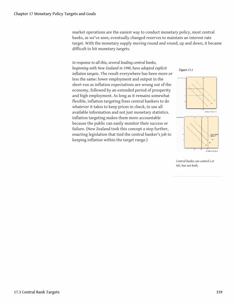
Figure 17.1
Central banks can control i orMS, but not both.
market operations are the easiest way to conduct monetary policy, most centralbanks, as we’ve seen, eventually changed reserves to maintain an interest ratetarget. With the monetary supply moving round and round, up and down, it becamedifficult to hit monetary targets.
In response to all this, several leading central banks,beginning with New Zealand in 1990, have adopted explicitinflation targets. The result everywhere has been more orless the same: lower employment and output in theshort run as inflation expectations are wrung out of theeconomy, followed by an extended period of prosperityand high employment. As long as it remains somewhatflexible, inflation targeting frees central bankers to dowhatever it takes to keep prices in check, to use allavailable information and not just monetary statistics.Inflation targeting makes them more accountablebecause the public can easily monitor their success orfailure. (New Zealand took this concept a step further,enacting legislation that tied the central banker’s job tokeeping inflation within the target range.)
Chapter 17 Monetary Policy Targets and Goals
17.3 Central Bank Targets 339
Stop and Think Box
What do you think of New Zealand’s law that allows the legislature to oust acentral banker who allows too much inflation?
Well, it makes the central bank less independent. Of course, independence isvaluable to the public only as a means of keeping inflation in check. The policyis only as good as the legislature. If it uses the punishment only to oustincompetent or corrupt central bankers, it should be salutary. If it ousts goodcentral bankers caught in a tough situation (for example, an oil supply shock orwar), the law may serve only to keep good people from taking the job. If thecentral banker’s salary is very high, the law might also induce him or her to tryto distort the official inflation figures on which his or her job depends.
The Fed has not yet adopted explicit inflation targeting, though a debate currently ragesabout whether it should. And under Ben Bernanke, it moved to what some have calledinflation targeting-lite, with a new policy of communicating with the public morefrequently about its forecasts, which now run to three years instead of thetraditional two.“The Federal Reserve: Letting Light In,” The Economist (17 November2007), 88–89. As noted above, the Fed is not very transparent, and that has theeffect of roiling the financial markets when expectations about its monetary policyturn out to be incorrect. It also induces people to waste a lot of time engaging in“Fed watching,” looking for clues about monetary policy. Reporters actually used tocomment on the thickness of Greenspan’s briefcase when he went into Federal OpenMarket Committee (FOMC) meetings. No joke!http://www.amazon.com/Inside-Greenspans-Briefcase-Investment-Strategies/dp/007138913X
Why doesn’t the Fed, which is charged with maintaining financial market and pricestability, adopt explicit targets? It may be that it does not want to be heldaccountable for its performance. It probably wants to protect its independence, butfor its private interest (power) rather than for the public interest (low inflation). Itmay also be that the Fed has found the holy grail of monetary policy, a flexible rule thathelps it to determine the appropriate federal funds target.
Chapter 17 Monetary Policy Targets and Goals
17.3 Central Bank Targets 340

KEY TAKEAWAYS
• Monetary targeting entails setting and attempting to meet growth ratesof monetary aggregates such as M1 or M2.
• It succeeded in countries like Germany and Switzerland, where thecentral bank was committed to keeping inflation in check.
• In other countries, like the United States and the United Kingdom,where price stability was not the paramount goal of the central bank,the time inconsistency problem eroded the effectiveness of the targets.
• In short, like a dieter who can’t resist that extra helping at dinner andtwo desserts, the central banks could not stick to a good long-term planday to day.
• Also, the connection between increases in particular aggregates and theprice level broke down, but it took a long time for central bankers torealize it because the lag between policy implementation and real-worldoutcome was often many months and sometimes years.
• Inflation targeting entails keeping increases in the price level within apredetermined range, e.g., 1 and 2 percent per year.
• Countries whose central banks embraced inflation targeting oftensuffered a recession and high unemployment at first, but in the long runwere able to achieve both price level stability and economic expansionand high employment.
• Inflation targeting makes use of all available information, not justmonetary aggregates, and increases the accountability of central banksand bankers. That reduces their independence but not at the expense ofhigher inflation because inflation targeting, in a sense, is a substitute forindependence.
Chapter 17 Monetary Policy Targets and Goals
17.3 Central Bank Targets 341
17.4 The Taylor Rule
LEARNING OBJECTIVE
1. What is the Taylor Rule and why is it important?
Many observers suspect that the Fed under Greenspan and Bernanke has followedthe so-called Taylor Rule, named after the Stanford University economist, JohnTaylor, who developed it. The rule2 states that
fft = π + ff*r + ½(π gap) + ½(Y gap)
where
fft = federal funds target
π = inflation
ff*r = the real equilibrium fed funds rate
π gap = inflation gap (π – π target)
Y gap = output gap (actual output [e.g. GDP] − output potential)
So if the inflation target was 2 percent, actual inflation was 3 percent, output was atits potential, and the real federal funds rate was 2 percent, the Taylor Rule suggeststhat the fed funds target should be
fft = π + ff*r + ½(π gap) + ½(Y gap)
fft = 3 + 2 + ½(1) + ½(0)
fft = 5.5
If the economy began running a percentage point below its potential, the TaylorRule would suggest easing monetary policy by lowering the fed funds target to 5percent:
2. In this context, a monetarypolicy rule, an equation thattells central bankers whatinterest rate policies theyshould put in place givenemployment, output, inflation,and perhaps othermacroeconomic variables.
Chapter 17 Monetary Policy Targets and Goals
342
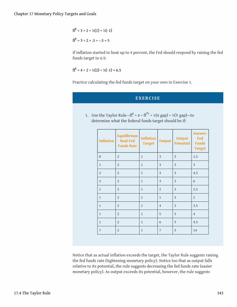
fft = 3 + 2 + ½(1) + ½(−1)
fft = 3 + 2 + .5 + −.5 = 5
If inflation started to heat up to 4 percent, the Fed should respond by raising the fedfunds target to 6.5:
fft = 4 + 2 + ½(2) + ½(−1) = 6.5
Practice calculating the fed funds target on your own in Exercise 1.
EXERCISE
1. Use the Taylor Rule—fft = π + ff*r + ½(π gap) + ½(Y gap)—todetermine what the federal funds target should be if:
InflationEquilibrium
Real FedFunds Rate
InflationTarget
OutputOutput
Potential
Answer:Fed
FundsTarget
0 2 1 3 3 1.5
1 2 1 3 3 3
2 2 1 3 3 4.5
3 2 1 3 3 6
1 2 1 2 3 2.5
1 2 1 1 3 2
1 2 1 4 3 3.5
1 2 1 5 3 4
1 2 1 6 3 4.5
7 2 1 7 3 14
Notice that as actual inflation exceeds the target, the Taylor Rule suggests raisingthe fed funds rate (tightening monetary policy). Notice too that as output fallsrelative to its potential, the rule suggests decreasing the fed funds rate (easiermonetary policy). As output exceeds its potential, however, the rule suggests
Chapter 17 Monetary Policy Targets and Goals
17.4 The Taylor Rule 343
putting on the brakes by raising rates. Finally, if inflation and output are bothscreaming, the rule requires that the fed funds target soar quite high indeed, as itdid in the early 1980s. In short, the Taylor Rule is countercyclical and accounts for twoimportant Federal Reserve goals: price stability and employment/output.
The Taylor Rule nicely explains U.S. macroeconomic history since 1960. In the early 1960s,the two were matched: inflation was low, and growth was strong. In the latter partof the 1960s, the 1970s, and the early 1980s, actual ff* was generally well below whatthe Taylor Rule said it should be. In that period, inflation was so high we refer tothe period as the Great Inflation. In the latter part of the 1980s, ff* was higher thanwhat the Taylor Rule suggested. That was a period of weak growth but decreasinginflation. From 1990 or so until the early 2000s, a period of low inflation and highgrowth, the Taylor Rule and ff* were very closely matched. In recent years,however, the Fed has generally kept ff* below the Rule.
Chapter 17 Monetary Policy Targets and Goals
17.4 The Taylor Rule 344

Stop and Think Box
Examine Figure 17.2 "The Fed’s feds fund target, 2003–2010" carefully.Assuming the Fed uses the Taylor Rule, what happened to inflation and outputfrom mid-2003 until mid-2006. Then what happened?
Figure 17.2The Fed’s feds fund target,2003–2010
Assuming that the Fed’s inflation target, the real equilibrium federal funds rate,and the economy’s output potential were unchanged in this period (not badassumptions), increases in actual inflation and increases in actual output wouldinduce the Fed, via the Taylor Rule, to increase its feds fund target. Both wereat play but were moderating by the end of 2006, freezing the funds target at5.25 percent, as shown in Figure 17.3 "Inflation and per capita gross domesticproduct (GDP), 2003–2006". Then the subprime mortgage crisis, recession, andPanic of 2008 struck, inducing the Fed quickly to lower its target to 3, then 2,then 1, then almost to zero.
Figure 17.3Inflation and per capita grossdomestic product (GDP),2003–2006
None of this means, however, that the Fed will continue to use the Taylor Rule, ifindeed it does so. Nor does it mean that the Taylor Rule will provide the right policy
Chapter 17 Monetary Policy Targets and Goals
17.4 The Taylor Rule 345
prescriptions in the future. Richard Fisher and W. Michael Cox, the president andchief economist of the Dallas Fed, respectively, believe that globalization makes itincreasingly important for the Fed and other central banks to look at worldinflation and output levels in order to get domestic monetary policy right.SeeRichard W. Fisher and W. Michael Cox, “The New Inflation Equation,” Wall StreetJournal, April 6, 2007, A11.
Stop and Think Box
Foreign exchange rates can also flummox central bankers and their policies.Specifically, increasing (decreasing) interest rates will, ceteris paribus, cause acurrency to appreciate (depreciate) in world currency markets. Why is thatimportant?
The value of a currency directly affects foreign trade. When a currency isstrong relative to other currencies (when each unit of it can purchase manyunits of foreign currencies), imports will be stimulated because foreign goodswill be cheap. Exports will be hurt, however, because domestic goods will lookexpensive to foreigners, who will have to give up many units of their localcurrency. Countries with economies heavily dependent on foreign trade mustbe extremely careful about the value of their currencies; almost every countryis becoming more dependent on foreign trade, making exchange rate policy anincreasingly important one for central banks worldwide to consider.
KEY TAKEAWAYS
• The Taylor Rule is a simple equation—fft = π + ff*r + ½( π gap) + ½(Ygap)—that allows central bankers to determine what their overnightinterbank lending rate target ought to be given actual inflation, aninflation target, actual output, the economy’s potential output, and anestimate of the equilibrium real fed funds rate.
• When the Fed has maintained the fed funds rate near that prescribed bythe Taylor Rule, the economy has thrived; when it has not, the economyhas been plagued by inflation (when the fed funds rate was set below theTaylor rate) or low output (when the fed funds rate was set above theTaylor rate).
Chapter 17 Monetary Policy Targets and Goals
17.4 The Taylor Rule 346
17.5 Suggested Reading
Blinder, Alan. Central Banking in Theory and Practice. Cambridge, MA: MIT Press, 1999.
Silber, William. When Washington Shut Down Wall Street: The Great Financial Crisis of1914 and the Origins of America’s Monetary Supremacy. Princeton, NJ: PrincetonUniversity Press, 2007.
Taylor, John B. Monetary Policy Rules. Chicago, IL: University of Chicago Press, 2001.
Chapter 17 Monetary Policy Targets and Goals
347
Chapter 18
Foreign Exchange
CHAPTER OBJECTIVES
By the end of this chapter, students should be able to:
1. Define foreign exchange and explain its importance.2. Describe the market for foreign exchange.3. Explain why countries shouldn’t be proud that it takes many units of
foreign currencies to purchase a single unit of their currency.4. Define purchasing power parity and explain its importance.5. List and explain the long-run determinants of exchange rates.6. List and explain the short-run determinants of exchange rates.7. Define the interest parity condition and explain when and why it holds.
348
18.1 The Economic Importance of Currency Markets
LEARNING OBJECTIVE
1. What is foreign exchange and why is it important?
Before we turn to monetary theory (gulp!) in Chapter 20 "Money Demand", there isone more real-world financial market we need to investigate in this and the nextchapter, the market for foreign currencies or foreign exchange, where the relativeprices of national units of account or exchange rates are determined. Why shouldyou care how many U.S. dollars (USD) it takes to buy a euro or a yen, a pound(sterling) or a dollar (of Canada or Australia, respectively)? If you plan to travel toany of those places, you’ll want to know so you can evaluate prices. Is €1,000 a goodprice for a hotel room? How about ¥1,000?The symbol for the euro, the currency ofthe European Union, is €. The symbol for the Japanese yen is ¥. But even if you remainyour entire life in a small village in Alaska, one of Hawaii’s outer islands, Michigan’s UpperPeninsula, or the northern reaches of Maine, the value of USD will affect your life deeply,whether you know it or not. Come again? How could that possibly be?
Every nation in the world trades with other nations. Some trade more than others(little islands like Iceland, Mauritius, and Ireland lead the way, in percentage ofgross domestic product [GDP] terms anyway) but all do it, even illicitly, when theUnited Nations says that they can’t because they’ve beenbad.http://www.entemp.ie/trade/export/sanctions.htm#overview We know fromChapter 3 "Money" that conducting trade via barter isn’t practical in mostcircumstances. So we use money. But what happens when people who want to trade usedifferent types of money, when their units of account are not the same? There are severalsolutions to that problem. The most frequent solution today is for one party, usuallythe buyer, to exchange the money of his or her country for the money of the seller’scountry, then to consummate the transaction.
How does this affect you? Well, when the unit of account of your country, say, U.S.dollars (USD or plain $), is strong, when it can buy many units of a foreign currency,say, Canadian dollars (C$), Canadian goods look cheap to you. And we all know whathappens when goods are cheap. So you stop drinking Bud and start drinkingMoosehead. Instead of going to Manhattan to shop, you go to Toronto, and checkout some Maple Leafs, Raptors, and Blue Jays games while you’re at it. (You go inApril, that magical month for sports fans.) When the Blue Jays game gets snowedout, you go instead to the Canadian ballet. (Do you have any sense of humor at all?)
Chapter 18 Foreign Exchange
349
You might even consider buying a Canadian computer or automobile. (Okay, let’snot get crazy.) The point is you and your fellow Americans import more from Canada.
The Canadians are very happy about this, but they are not so thrilled with Americangoods, which look dreadfully expensive to them because they have to give up manyof their dear loonies to buy USD. So they too eschew Manhattan for Toronto anddrink Moosehead rather than Bud. In other words, U.S. exports to Canada fall. Andbecause Canada is a major U.S. trading partner, that does not bode well for the U.S.economy overall, or U.S. residents, even those in remote villages. If USD were tocontinue to appreciate (strengthen, buy yet more C$), the situation would growincreasingly worse. Were the dollar to depreciate (weaken, buy fewer C$), the situationwould ameliorate and eventually reverse, and you’d go back to Bud, Manhattan shoppingsprees, and the Yankees, Mets, Knicks, Nets, Islanders, and Rangers.
Stop and Think Box
A chain of pizza parlors in the southwestern part of the United States acceptsMexican pesos in payment for its pizzas. Many U.S. retail stores located nearthe Canadian border accept Canadian currency. (Many Canadian businessesaccept U.S. dollars, too.) Why do these businesses accept payment in a foreigncurrency?
Well, maybe they are good folks who want to help out others and maybe someof them need foreign currencies to purchase supplies. But those are at bestulterior motives in most instances because the exchange rate offered usuallyheavily favors the retailer. For example, the pizza parlor’s exchange rate was 12pesos to the dollar when the market exchange rate was closer to 11. So a $10pizza costs 120 pesos (10 × 12) instead of 110 pesos (10 × 11). In short, it makes atidy and largely riskless profit from the offer.
Or imagine you don’t have many assets or a high income, but you need anautomobile. You see a commercial that says that there are three V-dubs (German-made Volkswagen automobile models) under $17,000. You think you can afford thatand begin to make arrangements to buy a Rabbit. But look in Figure 18.1 "The dollarprice of a €17,000 Rabbit and the euro price of a $10 computer fan" at what happensto the dollar price of a Rabbit when the exchange rate changes. Say that the Rabbitof your dreams costs €17,000. When the dollar and the euro are at parity (1 to 1), theRabbit costs $17,000. If the dollar depreciates (buys fewer euro, and more USD areneeded to buy €1), the Rabbit grows increasingly costly to you. If the dollar
Chapter 18 Foreign Exchange
18.1 The Economic Importance of Currency Markets 350

appreciates (buys more euro, and fewer USD are needed to buy €1), that coolautomotive bunny gets very cheap indeed!
Figure 18.1 The dollar price of a €17,000 Rabbit and the euro price of a $10 computer fan
Now imagine that in your remote little town you make fans for French computersthat you can sell profitably for $10.00. The dollar’s movements will affect you as aproducer, but in precisely the opposite way as it affected you as a consumer. Whenthe dollar appreciates against the euro, your computer fans grow more expensive inFrance (and indeed the entire euro zone), which will undoubtedly cut into sales andmaybe your salary or your job. When the dollar depreciates, the euro price of yourfans plummet, sales become increasingly brisk, and you think about buying aCadillac (a more expensive American car).
KEY TAKEAWAYS
• Foreign exchange is the trading of different national currencies or unitsof account.
• It is important because the exchange rate, the price of one currency interms of another, is a major determinant of a nation’s economic healthand hence the well-being of all the people residing in it.
Chapter 18 Foreign Exchange
18.1 The Economic Importance of Currency Markets 351
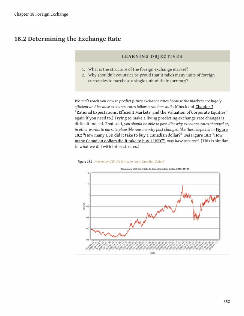
18.2 Determining the Exchange Rate
LEARNING OBJECTIVES
1. What is the structure of the foreign exchange market?2. Why shouldn’t countries be proud that it takes many units of foreign
currencies to purchase a single unit of their currency?
We can’t teach you how to predict future exchange rates because the markets are highlyefficient and because exchange rates follow a random walk. (Check out Chapter 7"Rational Expectations, Efficient Markets, and the Valuation of Corporate Equities"again if you need to.) Trying to make a living predicting exchange rate changes isdifficult indeed. That said, you should be able to post-dict why exchange rates changed or,in other words, to narrate plausible reasons why past changes, like those depicted in Figure18.2 "How many USD did it take to buy 1 Canadian dollar?" and Figure 18.3 "Howmany Canadian dollars did it take to buy 1 USD?", may have occurred. (This is similarto what we did with interest rates.)
Figure 18.2 How many USD did it take to buy 1 Canadian dollar?
Chapter 18 Foreign Exchange
352
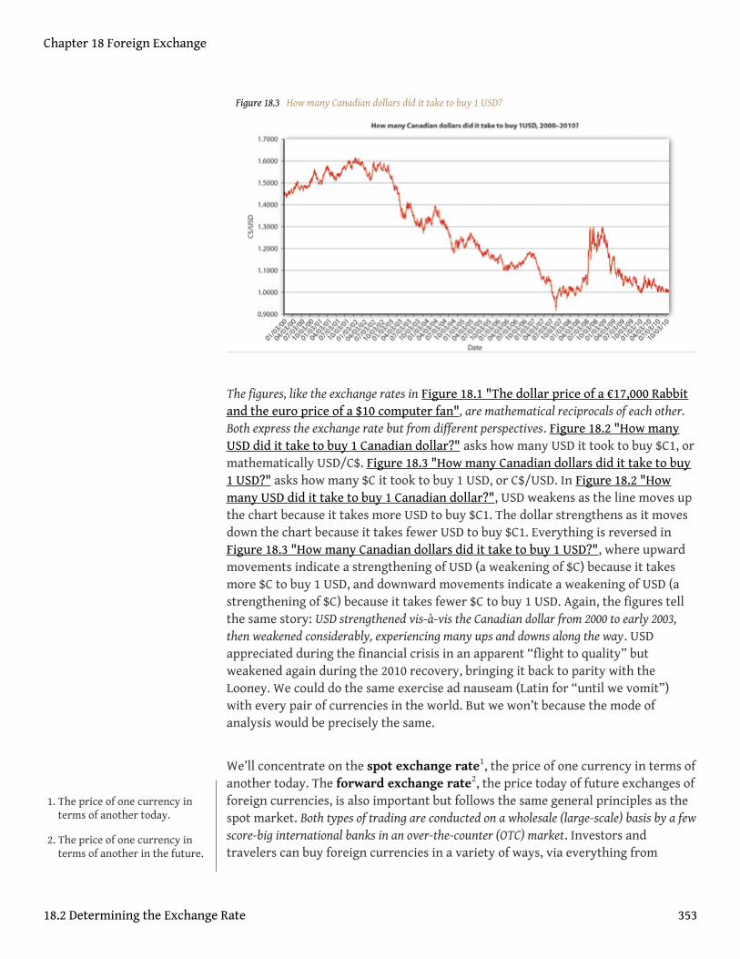
Figure 18.3 How many Canadian dollars did it take to buy 1 USD?
The figures, like the exchange rates in Figure 18.1 "The dollar price of a €17,000 Rabbitand the euro price of a $10 computer fan", are mathematical reciprocals of each other.Both express the exchange rate but from different perspectives. Figure 18.2 "How manyUSD did it take to buy 1 Canadian dollar?" asks how many USD it took to buy $C1, ormathematically USD/C$. Figure 18.3 "How many Canadian dollars did it take to buy1 USD?" asks how many $C it took to buy 1 USD, or C$/USD. In Figure 18.2 "Howmany USD did it take to buy 1 Canadian dollar?", USD weakens as the line moves upthe chart because it takes more USD to buy $C1. The dollar strengthens as it movesdown the chart because it takes fewer USD to buy $C1. Everything is reversed inFigure 18.3 "How many Canadian dollars did it take to buy 1 USD?", where upwardmovements indicate a strengthening of USD (a weakening of $C) because it takesmore $C to buy 1 USD, and downward movements indicate a weakening of USD (astrengthening of $C) because it takes fewer $C to buy 1 USD. Again, the figures tellthe same story: USD strengthened vis-à-vis the Canadian dollar from 2000 to early 2003,then weakened considerably, experiencing many ups and downs along the way. USDappreciated during the financial crisis in an apparent “flight to quality” butweakened again during the 2010 recovery, bringing it back to parity with theLooney. We could do the same exercise ad nauseam (Latin for “until we vomit”)with every pair of currencies in the world. But we won’t because the mode ofanalysis would be precisely the same.
We’ll concentrate on the spot exchange rate1, the price of one currency in terms ofanother today. The forward exchange rate2, the price today of future exchanges offoreign currencies, is also important but follows the same general principles as thespot market. Both types of trading are conducted on a wholesale (large-scale) basis by a fewscore-big international banks in an over-the-counter (OTC) market. Investors andtravelers can buy foreign currencies in a variety of ways, via everything from
1. The price of one currency interms of another today.
2. The price of one currency interms of another in the future.
Chapter 18 Foreign Exchange
18.2 Determining the Exchange Rate 353

brokerage accounts to airport kiosks, to their credit cards. Retail purchasers give upmore of their domestic currency to receive a given number of units of a foreigncurrency than the wholesale banks do. (To put the same idea another way, theyreceive fewer units of the foreign currency for each unit of their domesticcurrency.) That’s partly why the big banks are in the business. The big boys also tryto earn profits via speculation, buying (selling) a currency when it is low (high), andselling (buying) it when it is high (low). (They also seek out arbitrage opportunities,but those are rare and fleeting.) Each day, over $1 trillion of wholesale-level ($1million plus per transaction) foreign exchange transactions take place.
Before we go any further, a few words of caution. Students sometimes think that astrong currency is always better than a weak one. That undoubtedly stems from thefact that strong sounds good and weak sounds bad. As noted above, however, astrong (weak) currency is neither good nor bad but rather advantageous(disadvantageous) for imports/consumers and disadvantageous (advantageous) forexports/producers of exportable goods and services. Another thing: no need tothump your chest patriotically because it takes many units of foreign currencies to buy 1USD. That would be like proclaiming that you are “hot” because your temperature is98.6 degrees Fahrenheit instead of 37 degrees Centigrade (that’s the sametemperature, measured two different ways) or that you are 175 centimeters tallinstead of 68.9 inches (another equivalent). Most countries have a very small unit ofaccount compared to the United States, that is all. Other countries, like GreatBritain, have units of account that are larger than the USD, so it takes more than 1USD to buy a unit of those currencies. The nominal level of the exchange rate in noway means that one country or economy is better than another. Changes in exchangerates, by contrast, have profound consequences, as we have seen. They also have profoundcauses.
Chapter 18 Foreign Exchange
18.2 Determining the Exchange Rate 354
KEY TAKEAWAYS
• At the wholesale level, the market for foreign exchange is conducted bya few score large international players in huge (> $1 trillion per day)over-the-counter spot and forward markets.
• Those markets appear to be efficient in the sense that exchange ratesfollow a random walk and arbitrage opportunities, which appearinfrequently, are quickly eliminated.
• In the retail segment of the market, tourists, business travelers, andsmall-scale investors buy and sell foreign currencies, including physicalmedia of exchange (paper notes and coins), where appropriate.
• Compared to the wholesale ($1 million plus per transaction) players,retail purchasers of a foreign currency obtain fewer units of the foreigncurrency, and retail sellers of a foreign currency receive fewer units oftheir domestic currency.
• The nominal level of exchange rates is essentially arbitrary. Somecountries simply chose a smaller unit of account, a smaller amount ofvalue. That’s why it often takes over ¥100 to buy 1 USD. But if the UnitedStates had chosen a smaller unit of account, like a cent, or if Japan hadchosen a larger one (like ¥100 = ¥1), the yen and USD (and the euro, as itturns out) would be roughly at parity.
• A strong currency is not necessarily a good thing because it promotesimports over exports (because it makes foreign goods look so cheap anddomestic goods look so expensive to foreigners).
• A weak currency, despite the loser-sound to it, means strong exportsbecause domestic goods now look cheap both at home and abroad.Imports will decrease, too, because foreign goods will look moreexpensive to domestic consumers and businesses.
Chapter 18 Foreign Exchange
18.2 Determining the Exchange Rate 355

18.3 Long-Run Determinants of Exchange Rates
LEARNING OBJECTIVES
1. What is purchasing power parity?2. What are the other long-run determinants of exchange rates?
If transaction costs are zero, identical goods should have the same price no matter what unitof account that price is expressed in. Or so says the law of one price. The reason is clear: ifthey did not, arbitrageurs would buy where the good was cheapest and sell where itwas highest until the prices were equalized. Where transaction costs are nontrivialor goods are similar but not identical, we don’t expect a single price, but rather aband or range of prices. So if product X cost $100 in Country Y and $110 in CountryZ, and it costs $10 to transport X from Y to Z, there would be no arbitrageopportunity and the price differential could persist. If the price of X rose in Z to$120, we’d expect it to increase in Y to at least $110, or arbitrageurs would startbuying it in Y and selling it in Z until the prices were within $10 of each other.Similarly, Japanese-style beer is not the same as U.S.-style beer. But it is closeenough that we would not expect the prices to vary widely or otherwise consumerswould dump Bud, Miller, and Coors in favor of Kirin and Sapporo (or vice versa, asthe case may be).
This sort of analysis has led economists to apply the law of one price to entireeconomies in what they call the theory of purchasing power parity (PPP), which predictsthat, in the long run, exchange rates will reflect price level changes. In other words,higher rates of inflation in Country A compared to Country B will cause Country A’scurrency to depreciate vis-à-vis Country B’s currency in the long run. In the shortrun, however, matters are quite different, as Figure 18.4 "Purchasing power parity,United Kingdom and United States, 1975–2005" shows. If PPP held in the short run,USD should have appreciated against the pound (the blue line should be above zero)every year in which inflation in the United Kingdom exceeded inflation in theUnited States (the red line is above zero), and vice versa. Clearly, that was not thecase. But PPP has the long-run right, in sign but not quite in magnitude. Between 1975and 2005, prices rose in Great Britain a shade under 205 percent all told. In thatsame period, they rose just under 142 percent in the United States. In other words,prices rose about 44 percent ([205 − 142]/142) more in Britain than in the UnitedStates. Over that same period, the pound sterling depreciated 22 percent againstUSD (from £.4505 to £.5495 per USD or from $2.22 to $1.82 per £1), just as PPPtheory predicts it should have. But why the discrepancy in magnitude?
Chapter 18 Foreign Exchange
356
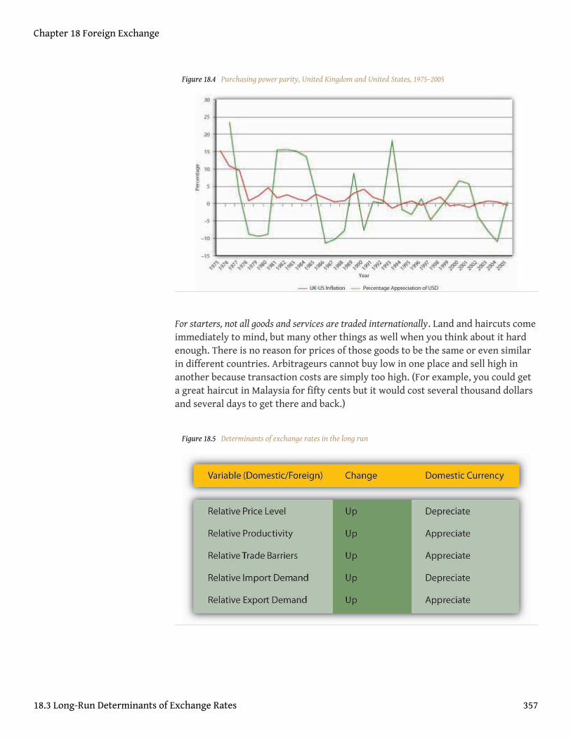
Figure 18.4 Purchasing power parity, United Kingdom and United States, 1975–2005
For starters, not all goods and services are traded internationally. Land and haircuts comeimmediately to mind, but many other things as well when you think about it hardenough. There is no reason for prices of those goods to be the same or even similarin different countries. Arbitrageurs cannot buy low in one place and sell high inanother because transaction costs are simply too high. (For example, you could geta great haircut in Malaysia for fifty cents but it would cost several thousand dollarsand several days to get there and back.)
Figure 18.5 Determinants of exchange rates in the long run
Chapter 18 Foreign Exchange
18.3 Long-Run Determinants of Exchange Rates 357
In addition, three other factors affect exchange rates in the long run: relative trade barriers,differential preferences for domestic and foreign goods, and differences in productivity.Tariffs (taxes on imported goods), quotas (caps on the quantity of imported goods),and sundry nontariff barriers (NTBs) to tradehttp://www.wto.org/english/thewto_e/whatis_e/tif_e/agrm9_e.htm increase demand for domestic over foreigngoods, thereby allowing the domestic currency to appreciate without injuring salesof domestic goods. Preferences for domestic goods have the same effect;preferences for foreign goods (French wine, German beer, Japanese automobiles)have the opposite effect, depreciating the domestic currency by maintainingdemand for foreign goods even in the face of higher prices. Finally, as a countrybecomes relatively more productive than other countries, the price of its warestends to fall. Its currency, therefore, appreciates because it can do so withoutinjuring exports. If a country’s productivity lags that of other countries, bycontrast, its currency will depreciate. Of course, this is all ceteris paribus. Figure18.5 "Determinants of exchange rates in the long run" summarizes the discussion.
Chapter 18 Foreign Exchange
18.3 Long-Run Determinants of Exchange Rates 358
KEY TAKEAWAYS
• Purchasing power parity (PPP) is the application of the law of one priceto entire economies.
• It predicts that exchange rates will adjust to relative price level changes,to differential inflation rates between two countries. They indeed do,but only in the long run and not to precisely the same degree.
• In the long run, exchange rates are determined by PPP (as describedabove) and relative differences in productivity, trade barriers, andimport and export demand.
• As Country A’s price level and import demand increase, and as CountryA’s productivity, trade barriers, and export demand decrease vis-à-visanother Country B, Country A’s currency depreciates and Country B’sappreciates.
• Basically, anything that lowers demand for Country A’s goods, services,and currency induces the currency to depreciate; anything thatincreases demand for Country A’s stuff induces the currency toappreciate in response.
• Higher inflation relative to Country B makes Country A’s stuff look moreexpensive, lowering demand and inducing depreciation.
• If economic actors in Country A take a fancy to Country B’s stuff, theywill import it even if Country A’s currency weakens, making Country B’sstuff more expensive. Reductions in trade barriers (lower tariffs, higherquotas, fewer NTBs) will exacerbate that.
• If, for whatever reason, economic actors in Country B don’t like CountryA’s stuff as much as they used to, they’ll buy less of it unless Country A’scurrency depreciates, making it cheaper.
• Finally, if Country A’s productivity slips relative to Country B’s, CountryA’s goods and services will get more expensive than Country B’s so it willsell in Country B only if its currency depreciates.
Chapter 18 Foreign Exchange
18.3 Long-Run Determinants of Exchange Rates 359
18.4 Short-Run Determinants of Exchange Rates
LEARNING OBJECTIVES
1. What are the short-run determinants of exchange rates?2. What is the interest parity condition and when and why does it hold?
As Figure 18.6 "South Africa-United States exchange rate, June 2006" shows,exchange rates can be very volatile. In a single month (June 2006), the South Africanrand depreciated from about 6.6 to 7.4 rand to 1 USD, with various ups and downsalong the way. The rand then reversed course and appreciated toward 7.1 rand/USD. Such fluctuations are by no means unusual. Why do exchange rates undergosuch gyrations? Figure 18.7 "Determinants of exchange rates in the short run"summarizes the major factors affecting exchange rates in the short run. Note that itlooks very much like Figure 18.5 "Determinants of exchange rates in the long run" butwith three key differences. First, instead of actual relative price levels, trade barriers,exports, imports, and productivity driving changes, expectations of their futuredirection drive changes. Given the discussion in Chapter 7 "Rational Expectations,Efficient Markets, and the Valuation of Corporate Equities", this should not besurprising. Second, two additional variables have entered the equation: foreign anddomestic interest rates. The intuition behind the first variables is the same as thosediscussed above, but in the short run, the mere expectation of a change in a variablemoves the market. The intuition behind the interest rates is also straightforward. Ifsomething increases demand for the domestic currency, like domestic interest ratesincreasing or foreign interest rates decreasing, it will appreciate. If something reducesdemand for the domestic currency, like domestic interest rates decreasing orforeign interest rates increasing, it will depreciate. (If this doesn’t make sense toyou, review the discussion in Chapter 5 "The Economics of Interest-RateFluctuations" regarding the theory of asset demand.) Because expectations andinterest rates change frequently, so, too, do exchange rates under the currentfloating rate regime.
Chapter 18 Foreign Exchange
360
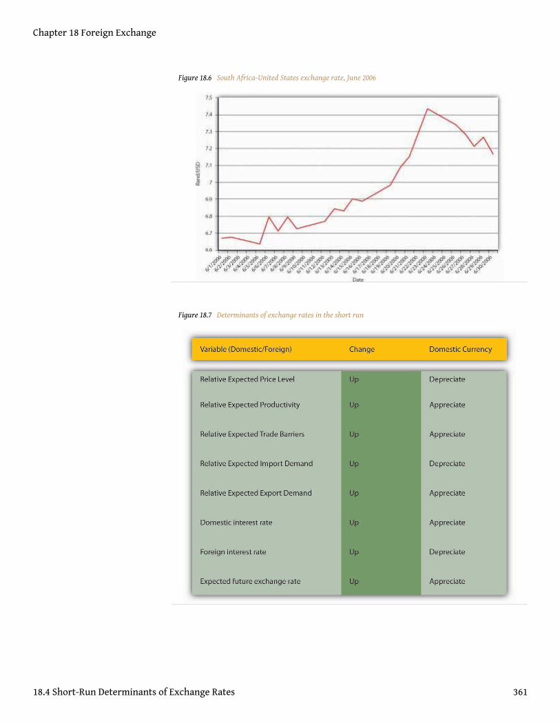
Figure 18.6 South Africa-United States exchange rate, June 2006
Figure 18.7 Determinants of exchange rates in the short run
Chapter 18 Foreign Exchange
18.4 Short-Run Determinants of Exchange Rates 361
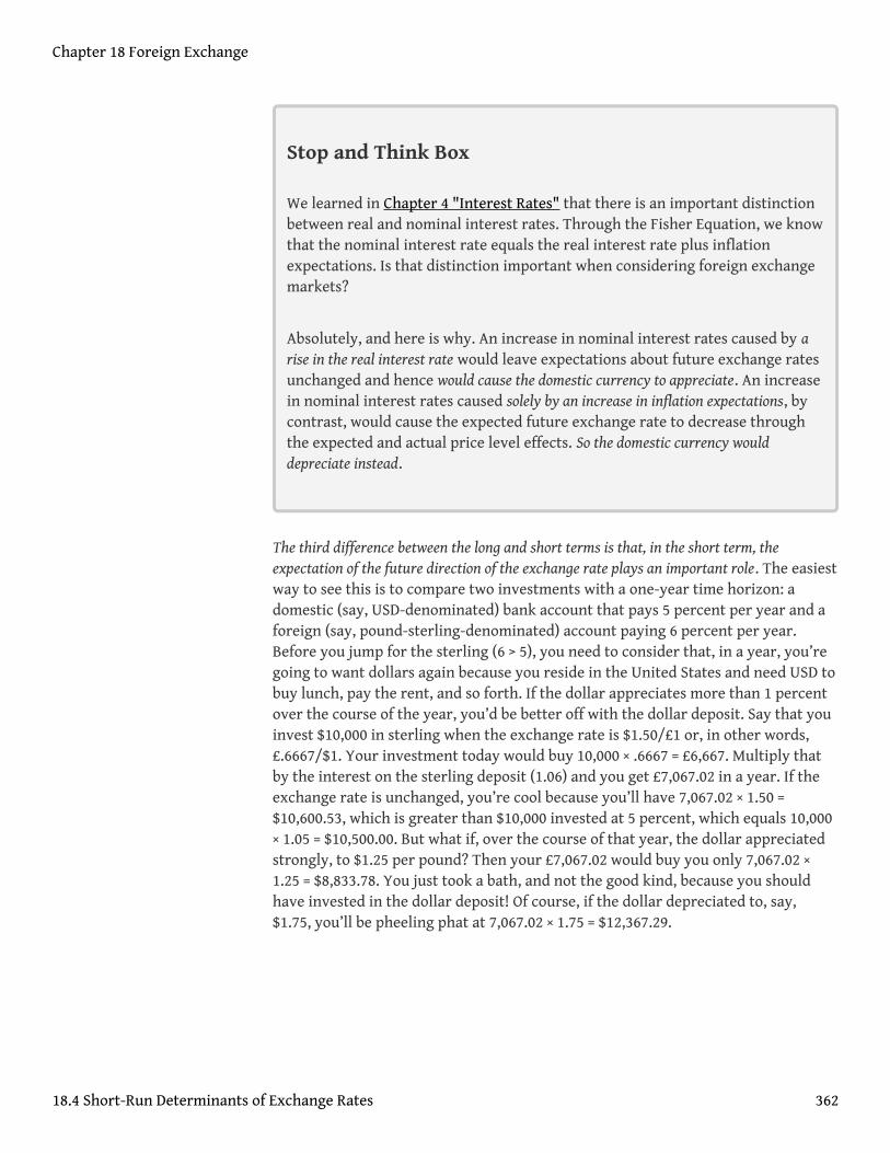
Stop and Think Box
We learned in Chapter 4 "Interest Rates" that there is an important distinctionbetween real and nominal interest rates. Through the Fisher Equation, we knowthat the nominal interest rate equals the real interest rate plus inflationexpectations. Is that distinction important when considering foreign exchangemarkets?
Absolutely, and here is why. An increase in nominal interest rates caused by arise in the real interest rate would leave expectations about future exchange ratesunchanged and hence would cause the domestic currency to appreciate. An increasein nominal interest rates caused solely by an increase in inflation expectations, bycontrast, would cause the expected future exchange rate to decrease throughthe expected and actual price level effects. So the domestic currency woulddepreciate instead.
The third difference between the long and short terms is that, in the short term, theexpectation of the future direction of the exchange rate plays an important role. The easiestway to see this is to compare two investments with a one-year time horizon: adomestic (say, USD-denominated) bank account that pays 5 percent per year and aforeign (say, pound-sterling-denominated) account paying 6 percent per year.Before you jump for the sterling (6 > 5), you need to consider that, in a year, you’regoing to want dollars again because you reside in the United States and need USD tobuy lunch, pay the rent, and so forth. If the dollar appreciates more than 1 percentover the course of the year, you’d be better off with the dollar deposit. Say that youinvest $10,000 in sterling when the exchange rate is $1.50/£1 or, in other words,£.6667/$1. Your investment today would buy 10,000 × .6667 = £6,667. Multiply thatby the interest on the sterling deposit (1.06) and you get £7,067.02 in a year. If theexchange rate is unchanged, you’re cool because you’ll have 7,067.02 × 1.50 =$10,600.53, which is greater than $10,000 invested at 5 percent, which equals 10,000× 1.05 = $10,500.00. But what if, over the course of that year, the dollar appreciatedstrongly, to $1.25 per pound? Then your £7,067.02 would buy you only 7,067.02 ×1.25 = $8,833.78. You just took a bath, and not the good kind, because you shouldhave invested in the dollar deposit! Of course, if the dollar depreciated to, say,$1.75, you’ll be pheeling phat at 7,067.02 × 1.75 = $12,367.29.
Chapter 18 Foreign Exchange
18.4 Short-Run Determinants of Exchange Rates 362
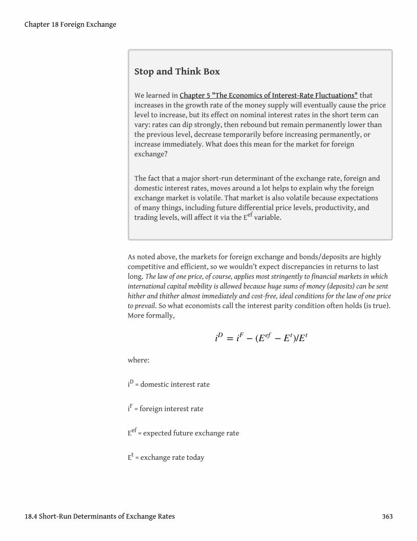
Stop and Think Box
We learned in Chapter 5 "The Economics of Interest-Rate Fluctuations" thatincreases in the growth rate of the money supply will eventually cause the pricelevel to increase, but its effect on nominal interest rates in the short term canvary: rates can dip strongly, then rebound but remain permanently lower thanthe previous level, decrease temporarily before increasing permanently, orincrease immediately. What does this mean for the market for foreignexchange?
The fact that a major short-run determinant of the exchange rate, foreign anddomestic interest rates, moves around a lot helps to explain why the foreignexchange market is volatile. That market is also volatile because expectationsof many things, including future differential price levels, productivity, andtrading levels, will affect it via the Eef variable.
As noted above, the markets for foreign exchange and bonds/deposits are highlycompetitive and efficient, so we wouldn’t expect discrepancies in returns to lastlong. The law of one price, of course, applies most stringently to financial markets in whichinternational capital mobility is allowed because huge sums of money (deposits) can be senthither and thither almost immediately and cost-free, ideal conditions for the law of one priceto prevail. So what economists call the interest parity condition often holds (is true).More formally,
where:
iD = domestic interest rate
iF = foreign interest rate
Eef = expected future exchange rate
Et = exchange rate today
iD = iF − (Eef − E t)/E t
Chapter 18 Foreign Exchange
18.4 Short-Run Determinants of Exchange Rates 363
In plain English, if the so-called interest parity condition holds, the domestic interestrate should equal the foreign interest rate minus the expected appreciation of the domesticcurrency. If iF is > iD, the domestic currency must be expected to appreciate;otherwise, everyone would sell their domestic deposits to buy the foreign ones. If iF
is < iD, the domestic currency must be expected to depreciate (have a negative sign,two of which make a positive, augmenting iF); otherwise, everyone would sell theforeign deposits and buy the domestic ones. If you find this confusing, there isanother, more intuitive way of stating it: the domestic interest rate must equal theforeign interest rate plus the expected appreciation of the foreign currency. If iF is <iD, the expected appreciation of the foreign currency compensates for the lowerinterest rate, allowing equilibrium. You can practice calculating interest parity inExercise 1.
Chapter 18 Foreign Exchange
18.4 Short-Run Determinants of Exchange Rates 364
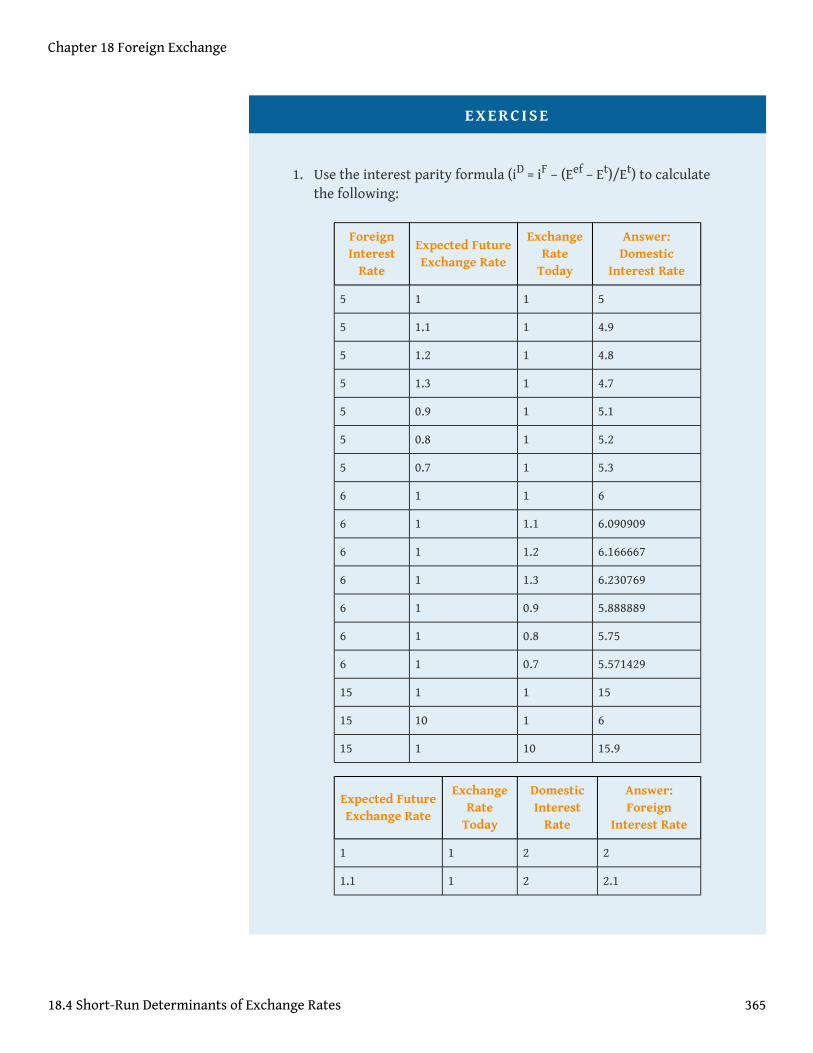
EXERCISE
1. Use the interest parity formula (iD = iF – (Eef – Et)/Et) to calculatethe following:
ForeignInterest
Rate
Expected FutureExchange Rate
ExchangeRate
Today
Answer:Domestic
Interest Rate
5 1 1 5
5 1.1 1 4.9
5 1.2 1 4.8
5 1.3 1 4.7
5 0.9 1 5.1
5 0.8 1 5.2
5 0.7 1 5.3
6 1 1 6
6 1 1.1 6.090909
6 1 1.2 6.166667
6 1 1.3 6.230769
6 1 0.9 5.888889
6 1 0.8 5.75
6 1 0.7 5.571429
15 1 1 15
15 10 1 6
15 1 10 15.9
Expected FutureExchange Rate
ExchangeRate
Today
DomesticInterest
Rate
Answer:Foreign
Interest Rate
1 1 2 2
1.1 1 2 2.1
Chapter 18 Foreign Exchange
18.4 Short-Run Determinants of Exchange Rates 365
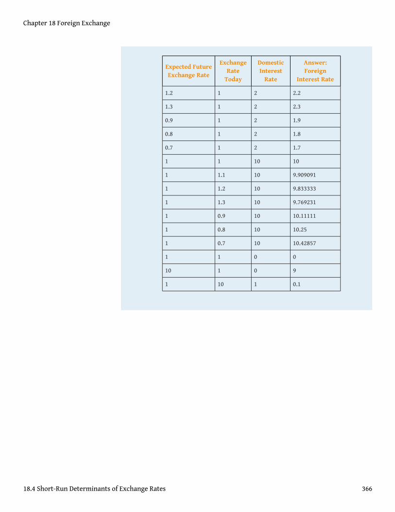
Expected FutureExchange Rate
ExchangeRate
Today
DomesticInterest
Rate
Answer:Foreign
Interest Rate
1.2 1 2 2.2
1.3 1 2 2.3
0.9 1 2 1.9
0.8 1 2 1.8
0.7 1 2 1.7
1 1 10 10
1 1.1 10 9.909091
1 1.2 10 9.833333
1 1.3 10 9.769231
1 0.9 10 10.11111
1 0.8 10 10.25
1 0.7 10 10.42857
1 1 0 0
10 1 0 9
1 10 1 0.1
Chapter 18 Foreign Exchange
18.4 Short-Run Determinants of Exchange Rates 366
KEY TAKEAWAYS
• Because foreign exchange markets are efficient, in the short run, themere expectation of changes in relative inflation, exports, imports,trade barriers, and productivity moves the markets.
• Also in the short run, differences in interest rates and expectations ofthe future exchange rate play key roles in exchange rate determination.
• The interest parity condition equates the domestic interest rate to theforeign interest rate minus the appreciation of the domestic currency.(Or, by rearranging the terms, it equates the foreign interest rate to thedomestic interest rate plus the expected appreciation of the domesticcurrency.)
• The interest parity condition holds whenever there is capital mobility,whenever deposits (units of account) can move freely and cheaply fromone country to another.
• It holds under those conditions because if it didn’t, an arbitragecondition would exist, inducing arbitrageurs to sell the overvalueddeposit (side of the equation) and buy the undervalued one until theequation held.
Chapter 18 Foreign Exchange
18.4 Short-Run Determinants of Exchange Rates 367
18.5 Modeling the Market for Foreign Exchange
LEARNING OBJECTIVE
1. How can the market for foreign exchange be modeled?
Like other markets, the market for foreign exchange can be graphically modeled to help usvisualize the action, as in Figure 18.8 "Equilibrium in the market for USD". There are anumber of ways to do this, but perhaps the easiest is to plot the quantity of dollarson the horizontal and the exchange rate, stated in terms of foreign divided bydomestic (say, yen or ¥/USD) on the vertical. The supply of dollar assets will beperfectly vertical, unchanged at every exchange rate. The demand for dollars, bycontrast, will have the usual downward slope because, at higher exchange rates,fewer dollar assets will be demanded than at lower exchange rates. So at ¥120 to 1USD, relatively few dollar-denominated assets will be demanded compared to only¥100 or ¥80 per dollar. The intersection of the supply and demand curves willdetermine E*, which in this case is ¥100/$, and q*, which in this case is $100 billion.
Chapter 18 Foreign Exchange
368
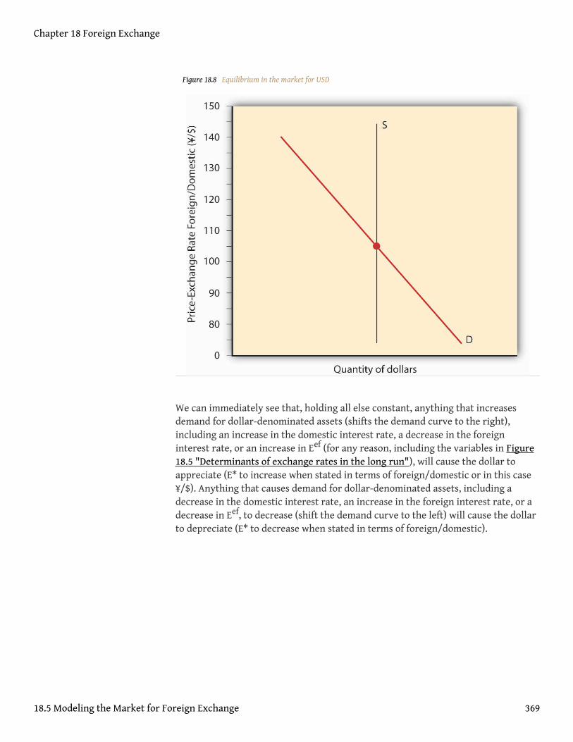
Figure 18.8 Equilibrium in the market for USD
We can immediately see that, holding all else constant, anything that increasesdemand for dollar-denominated assets (shifts the demand curve to the right),including an increase in the domestic interest rate, a decrease in the foreigninterest rate, or an increase in Eef (for any reason, including the variables in Figure18.5 "Determinants of exchange rates in the long run"), will cause the dollar toappreciate (E* to increase when stated in terms of foreign/domestic or in this case¥/$). Anything that causes demand for dollar-denominated assets, including adecrease in the domestic interest rate, an increase in the foreign interest rate, or adecrease in Eef, to decrease (shift the demand curve to the left) will cause the dollarto depreciate (E* to decrease when stated in terms of foreign/domestic).
Chapter 18 Foreign Exchange
18.5 Modeling the Market for Foreign Exchange 369
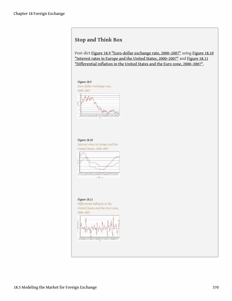
Stop and Think Box
Post-dict Figure 18.9 "Euro-dollar exchange rate, 2000–2007" using Figure 18.10"Interest rates in Europe and the United States, 2000–2007" and Figure 18.11"Differential inflation in the United States and the Euro zone, 2000–2007".
Figure 18.9Euro-dollar exchange rate,2000–2007
Figure 18.10Interest rates in Europe and theUnited States, 2000–2007
Figure 18.11Differential inflation in theUnited States and the Euro zone,2000–2007
Chapter 18 Foreign Exchange
18.5 Modeling the Market for Foreign Exchange 370
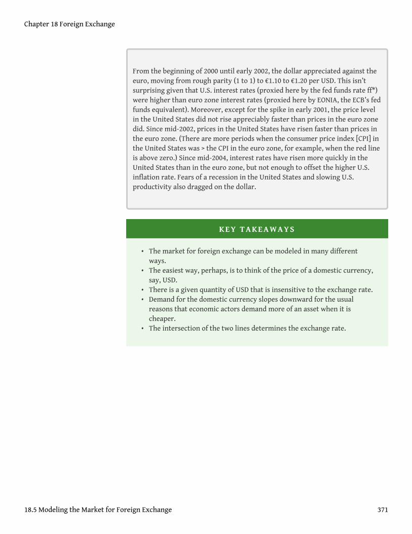
From the beginning of 2000 until early 2002, the dollar appreciated against theeuro, moving from rough parity (1 to 1) to €1.10 to €1.20 per USD. This isn’tsurprising given that U.S. interest rates (proxied here by the fed funds rate ff*)were higher than euro zone interest rates (proxied here by EONIA, the ECB’s fedfunds equivalent). Moreover, except for the spike in early 2001, the price levelin the United States did not rise appreciably faster than prices in the euro zonedid. Since mid-2002, prices in the United States have risen faster than prices inthe euro zone. (There are more periods when the consumer price index [CPI] inthe United States was > the CPI in the euro zone, for example, when the red lineis above zero.) Since mid-2004, interest rates have risen more quickly in theUnited States than in the euro zone, but not enough to offset the higher U.S.inflation rate. Fears of a recession in the United States and slowing U.S.productivity also dragged on the dollar.
KEY TAKEAWAYS
• The market for foreign exchange can be modeled in many differentways.
• The easiest way, perhaps, is to think of the price of a domestic currency,say, USD.
• There is a given quantity of USD that is insensitive to the exchange rate.• Demand for the domestic currency slopes downward for the usual
reasons that economic actors demand more of an asset when it ischeaper.
• The intersection of the two lines determines the exchange rate.
Chapter 18 Foreign Exchange
18.5 Modeling the Market for Foreign Exchange 371
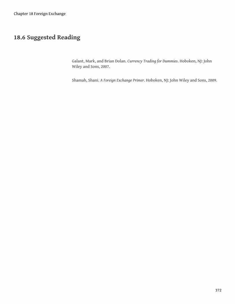
18.6 Suggested Reading
Galant, Mark, and Brian Dolan. Currency Trading for Dummies. Hoboken, NJ: JohnWiley and Sons, 2007.
Shamah, Shani. A Foreign Exchange Primer. Hoboken, NJ: John Wiley and Sons, 2009.
Chapter 18 Foreign Exchange
372
Chapter 19
International Monetary Regimes
CHAPTER OBJECTIVES
By the end of this chapter, students should be able to:
1. Define the impossible trinity, or trilemma, and explain its importance.2. Identify the four major types of international monetary regimes and
describe how they differ.3. Explain how central banks manage the foreign exchange (FX) rate.4. Explain the benefits of fixing the FX rate, or keeping it within a narrow
band.5. Explain the costs of fixing the FX rate, or keeping it in a narrow band.
373
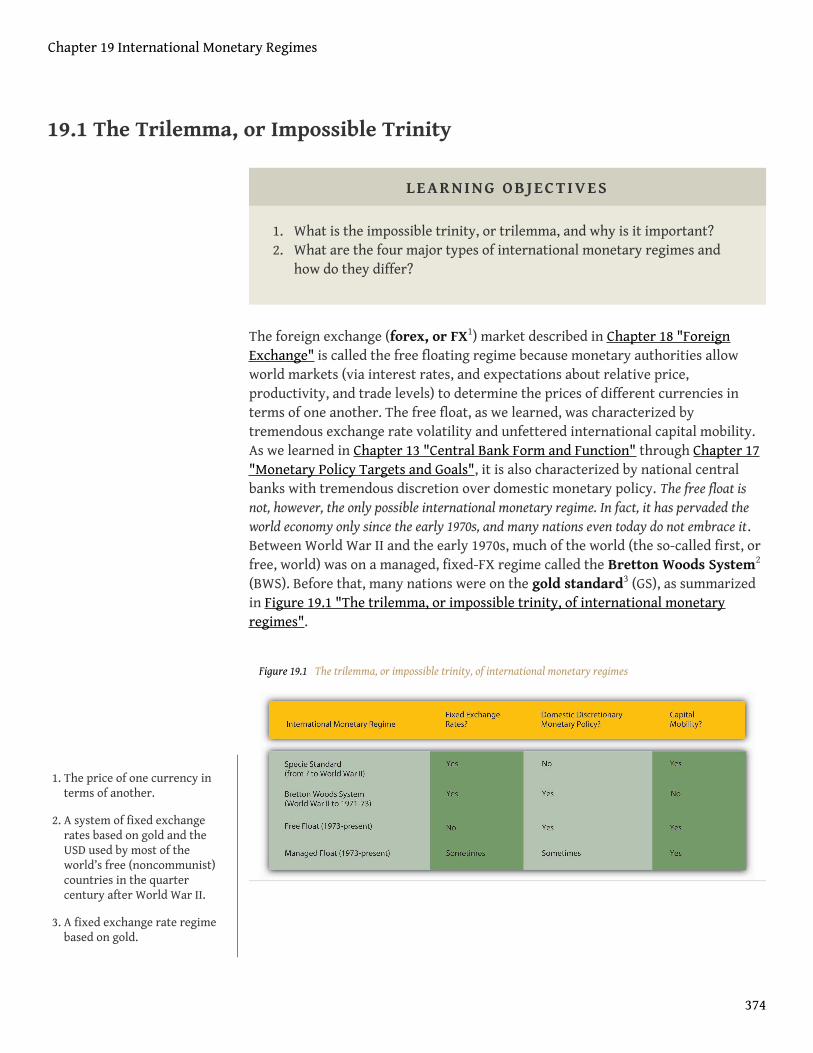
19.1 The Trilemma, or Impossible Trinity
LEARNING OBJECTIVES
1. What is the impossible trinity, or trilemma, and why is it important?2. What are the four major types of international monetary regimes and
how do they differ?
The foreign exchange (forex, or FX1) market described in Chapter 18 "ForeignExchange" is called the free floating regime because monetary authorities allowworld markets (via interest rates, and expectations about relative price,productivity, and trade levels) to determine the prices of different currencies interms of one another. The free float, as we learned, was characterized bytremendous exchange rate volatility and unfettered international capital mobility.As we learned in Chapter 13 "Central Bank Form and Function" through Chapter 17"Monetary Policy Targets and Goals", it is also characterized by national centralbanks with tremendous discretion over domestic monetary policy. The free float isnot, however, the only possible international monetary regime. In fact, it has pervaded theworld economy only since the early 1970s, and many nations even today do not embrace it.Between World War II and the early 1970s, much of the world (the so-called first, orfree, world) was on a managed, fixed-FX regime called the Bretton Woods System2
(BWS). Before that, many nations were on the gold standard3 (GS), as summarizedin Figure 19.1 "The trilemma, or impossible trinity, of international monetaryregimes".
Figure 19.1 The trilemma, or impossible trinity, of international monetary regimes
1. The price of one currency interms of another.
2. A system of fixed exchangerates based on gold and theUSD used by most of theworld’s free (noncommunist)countries in the quartercentury after World War II.
3. A fixed exchange rate regimebased on gold.
Chapter 19 International Monetary Regimes
374
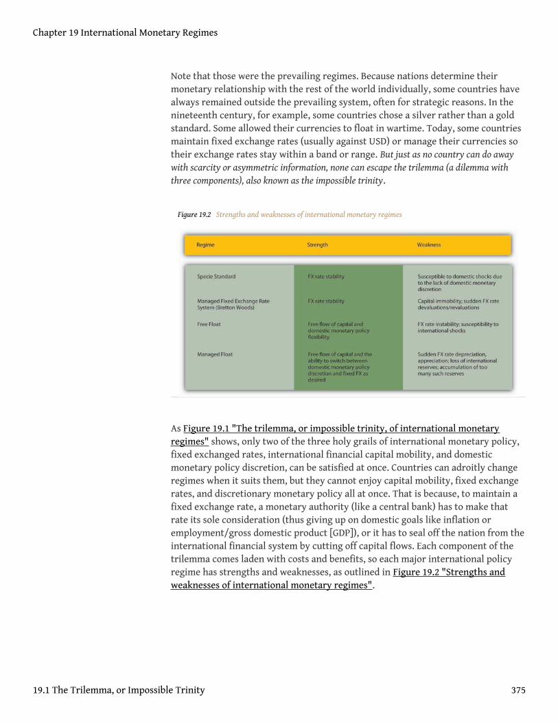
Note that those were the prevailing regimes. Because nations determine theirmonetary relationship with the rest of the world individually, some countries havealways remained outside the prevailing system, often for strategic reasons. In thenineteenth century, for example, some countries chose a silver rather than a goldstandard. Some allowed their currencies to float in wartime. Today, some countriesmaintain fixed exchange rates (usually against USD) or manage their currencies sotheir exchange rates stay within a band or range. But just as no country can do awaywith scarcity or asymmetric information, none can escape the trilemma (a dilemma withthree components), also known as the impossible trinity.
Figure 19.2 Strengths and weaknesses of international monetary regimes
As Figure 19.1 "The trilemma, or impossible trinity, of international monetaryregimes" shows, only two of the three holy grails of international monetary policy,fixed exchanged rates, international financial capital mobility, and domesticmonetary policy discretion, can be satisfied at once. Countries can adroitly changeregimes when it suits them, but they cannot enjoy capital mobility, fixed exchangerates, and discretionary monetary policy all at once. That is because, to maintain afixed exchange rate, a monetary authority (like a central bank) has to make thatrate its sole consideration (thus giving up on domestic goals like inflation oremployment/gross domestic product [GDP]), or it has to seal off the nation from theinternational financial system by cutting off capital flows. Each component of thetrilemma comes laden with costs and benefits, so each major international policyregime has strengths and weaknesses, as outlined in Figure 19.2 "Strengths andweaknesses of international monetary regimes".
Chapter 19 International Monetary Regimes
19.1 The Trilemma, or Impossible Trinity 375
Stop and Think Box
From 1797 until 1820 or so, Great Britain abandoned the specie standard4 ithad maintained for as long as anyone could remember and allowed the poundsterling to float quite freely. That was a period of almost nonstop warfareknown as the Napoleonic Wars. The United States also abandoned its speciestandard from 1775 until 1781, from 1814 until 1817, and from 1862 untilessentially 1873. Why?
Those were also periods of warfare and their immediate aftermath in theUnited States—the Revolution, War of 1812, and Civil War, respectively.Apparently during wartime, both countries found the specie standard costlyand preferred instead to float with free mobility of financial capital. Thatallowed them to borrow abroad while simultaneously gaining discretion overdomestic monetary policy, essentially allowing them to fund part of the cost ofthe wars with a currency tax, which is to say, inflation.
4. A fixed exchange rate regimebased on specie, i.e., gold and/or silver.
Chapter 19 International Monetary Regimes
19.1 The Trilemma, or Impossible Trinity 376
KEY TAKEAWAYS
• The impossible trinity, or trilemma, is one of those aspects of the natureof things, like scarcity and asymmetric information, that makes lifedifficult.
• Specifically, the trilemma means that a country can follow only two ofthree policies at once: international capital mobility, fixed exchangerates, and discretionary domestic monetary policy.
• To keep exchange rates fixed, the central bank must either restrictcapital flows or give up its control over the domestic money supply,interest rates, and price level.
• This means that a country must make difficult decisions about whichvariables it wants to control and which it wants to give up to outsideforces.
• The four major types of international monetary regime are speciestandard, managed fixed exchange rate, free float, and managed float.
• They differ in their solution, so to speak, of the impossible trinity.• Specie standards, like the classical GS, maintained fixed exchange rates
and allowed the free flow of financial capital internationally, renderingit impossible to alter domestic money supplies, interest rates, orinflation rates.
• Managed fixed exchange rate regimes like BWS allowed central banksdiscretion and fixed exchange rates at the cost of restrictinginternational capital flows.
• Under a free float, free capital flows are again allowed, as is domesticdiscretionary monetary policy, but at the expense of the security andstability of fixed exchange rates.
• With a managed float, that same solution prevails until the FX ratemoves to the top or bottom of the desired band, at which point thecentral bank gives up its domestic discretion so it can concentrate onappreciating or depreciating its currency.
Chapter 19 International Monetary Regimes
19.1 The Trilemma, or Impossible Trinity 377
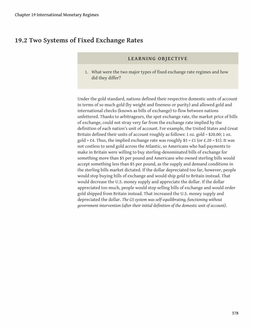
19.2 Two Systems of Fixed Exchange Rates
LEARNING OBJECTIVE
1. What were the two major types of fixed exchange rate regimes and howdid they differ?
Under the gold standard, nations defined their respective domestic units of accountin terms of so much gold (by weight and fineness or purity) and allowed gold andinternational checks (known as bills of exchange) to flow between nationsunfettered. Thanks to arbitrageurs, the spot exchange rate, the market price of billsof exchange, could not stray very far from the exchange rate implied by thedefinition of each nation’s unit of account. For example, the United States and GreatBritain defined their units of account roughly as follows: 1 oz. gold = $20.00; 1 oz.gold = £4. Thus, the implied exchange rate was roughly $5 = £1 (or £.20 = $1). It wasnot costless to send gold across the Atlantic, so Americans who had payments tomake in Britain were willing to buy sterling-denominated bills of exchange forsomething more than $5 per pound and Americans who owned sterling bills wouldaccept something less than $5 per pound, as the supply and demand conditions inthe sterling bills market dictated. If the dollar depreciated too far, however, peoplewould stop buying bills of exchange and would ship gold to Britain instead. Thatwould decrease the U.S. money supply and appreciate the dollar. If the dollarappreciated too much, people would stop selling bills of exchange and would ordergold shipped from Britain instead. That increased the U.S. money supply anddepreciated the dollar. The GS system was self-equilibrating, functioning withoutgovernment intervention (after their initial definition of the domestic unit of account).
Chapter 19 International Monetary Regimes
378
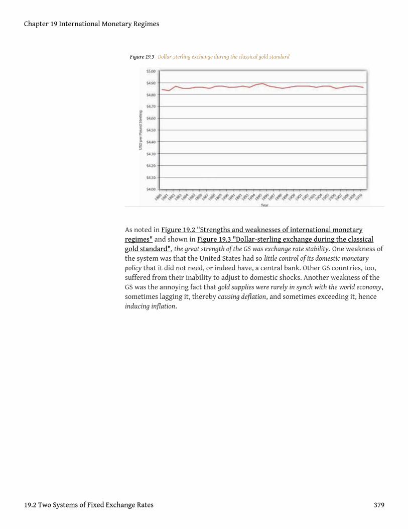
Figure 19.3 Dollar-sterling exchange during the classical gold standard
As noted in Figure 19.2 "Strengths and weaknesses of international monetaryregimes" and shown in Figure 19.3 "Dollar-sterling exchange during the classicalgold standard", the great strength of the GS was exchange rate stability. One weakness ofthe system was that the United States had so little control of its domestic monetarypolicy that it did not need, or indeed have, a central bank. Other GS countries, too,suffered from their inability to adjust to domestic shocks. Another weakness of theGS was the annoying fact that gold supplies were rarely in synch with the world economy,sometimes lagging it, thereby causing deflation, and sometimes exceeding it, henceinducing inflation.
Chapter 19 International Monetary Regimes
19.2 Two Systems of Fixed Exchange Rates 379
Stop and Think Box
Why did the United States find it prudent to have a central bank (the B.U.S.[1791–1811] and the S.B.U.S. [1816–1836]) during the late eighteenth and earlynineteenth centuries, when it was on a specie standard, but not later in thenineteenth century? (Hint: Transatlantic transportation technology improveddramatically beginning in the 1810s.)
As discussed in earlier chapters, the B.U.S. and S.B.U.S. had some control overthe domestic money supply by regulating commercial bank reserves via thealacrity of its note and deposit redemption policy. Although the United Stateswas on a de facto specie standard (legally bimetallic but de facto silver, thengold) at the time, the exchange rate bands were quite wide becausetransportation costs (insurance, freight, interest lost in transit) were so largecompared to later in the century that the U.S. monetary regime was more akinto a modern managed float. In other words, the central bank had discretion tochange the money supply and exchange rates within the wide band that thecostly state of technology created.
The Bretton Woods System adopted by the first world countries in the final stages ofWorld War II was designed to overcome the flaws of the GS while maintaining the stabilityof fixed exchange rates. By making the dollar the free world’s reserve currency (basicallysubstituting USD for gold), it ensured a more elastic supply of international reserves and alsoallowed the United States to earn seigniorage to help offset the costs it incurred fightingWorld War II, the Korean War, and the cold war. The U.S. government promised toconvert USD into gold at a fixed rate ($35 per oz.), essentially rendering the UnitedStates the banker to more than half of the world’s economy. The other countries inthe system maintained fixed exchange rates with the dollar and allowed fordomestic monetary policy discretion, so the BWS had to restrict internationalcapital flows. Little wonder that the period after World War II witnessed a massiveshrinkage of the international financial system.
Under the BWS, if a country could no longer defend its fixed rate with the dollar, itwas allowed to devalue its currency, or in other words, to set a newer, weakerexchange rate. As Figure 19.4 "Dollar–sterling exchange under BWS" reveals, GreatBritain devalued several times, as did other members of the BWS. But whatultimately destroyed the system was the fact that the banker, the United States,kept issuing more USD without increasing its reserve of gold. The internationalequivalent of a bank run ensued because major countries, led by France, exchanged
Chapter 19 International Monetary Regimes
19.2 Two Systems of Fixed Exchange Rates 380
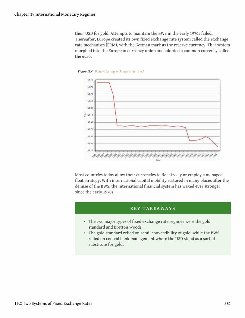
their USD for gold. Attempts to maintain the BWS in the early 1970s failed.Thereafter, Europe created its own fixed exchange rate system called the exchangerate mechanism (ERM), with the German mark as the reserve currency. That systemmorphed into the European currency union and adopted a common currency calledthe euro.
Figure 19.4 Dollar–sterling exchange under BWS
Most countries today allow their currencies to float freely or employ a managedfloat strategy. With international capital mobility restored in many places after thedemise of the BWS, the international financial system has waxed ever strongersince the early 1970s.
KEY TAKEAWAYS
• The two major types of fixed exchange rate regimes were the goldstandard and Bretton Woods.
• The gold standard relied on retail convertibility of gold, while the BWSrelied on central bank management where the USD stood as a sort ofsubstitute for gold.
Chapter 19 International Monetary Regimes
19.2 Two Systems of Fixed Exchange Rates 381
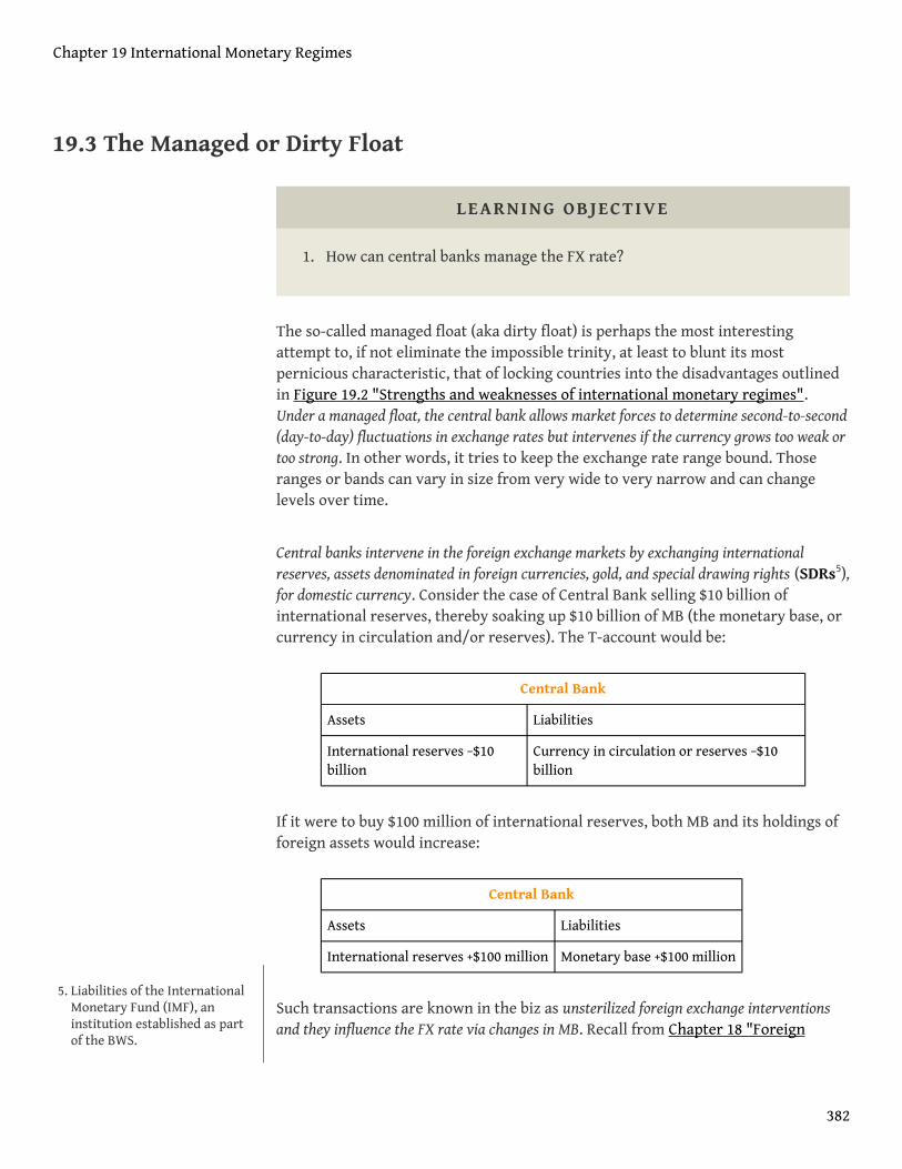
19.3 The Managed or Dirty Float
LEARNING OBJECTIVE
1. How can central banks manage the FX rate?
The so-called managed float (aka dirty float) is perhaps the most interestingattempt to, if not eliminate the impossible trinity, at least to blunt its mostpernicious characteristic, that of locking countries into the disadvantages outlinedin Figure 19.2 "Strengths and weaknesses of international monetary regimes".Under a managed float, the central bank allows market forces to determine second-to-second(day-to-day) fluctuations in exchange rates but intervenes if the currency grows too weak ortoo strong. In other words, it tries to keep the exchange rate range bound. Thoseranges or bands can vary in size from very wide to very narrow and can changelevels over time.
Central banks intervene in the foreign exchange markets by exchanging internationalreserves, assets denominated in foreign currencies, gold, and special drawing rights (SDRs5),for domestic currency. Consider the case of Central Bank selling $10 billion ofinternational reserves, thereby soaking up $10 billion of MB (the monetary base, orcurrency in circulation and/or reserves). The T-account would be:
Central Bank
Assets Liabilities
International reserves −$10billion
Currency in circulation or reserves −$10billion
If it were to buy $100 million of international reserves, both MB and its holdings offoreign assets would increase:
Central Bank
Assets Liabilities
International reserves +$100 million Monetary base +$100 million
Such transactions are known in the biz as unsterilized foreign exchange interventionsand they influence the FX rate via changes in MB. Recall from Chapter 18 "Foreign
5. Liabilities of the InternationalMonetary Fund (IMF), aninstitution established as partof the BWS.
Chapter 19 International Monetary Regimes
382
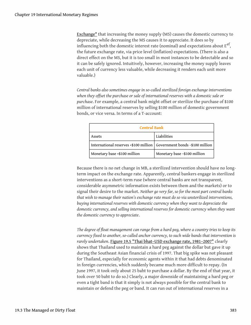
Exchange" that increasing the money supply (MS) causes the domestic currency todepreciate, while decreasing the MS causes it to appreciate. It does so byinfluencing both the domestic interest rate (nominal) and expectations about Eef,the future exchange rate, via price level (inflation) expectations. (There is also adirect effect on the MS, but it is too small in most instances to be detectable and soit can be safely ignored. Intuitively, however, increasing the money supply leaveseach unit of currency less valuable, while decreasing it renders each unit morevaluable.)
Central banks also sometimes engage in so-called sterilized foreign exchange interventionswhen they offset the purchase or sale of international reserves with a domestic sale orpurchase. For example, a central bank might offset or sterilize the purchase of $100million of international reserves by selling $100 million of domestic governmentbonds, or vice versa. In terms of a T-account:
Central Bank
Assets Liabilities
International reserves +$100 million Government bonds −$100 million
Monetary base +$100 million Monetary base −$100 million
Because there is no net change in MB, a sterilized intervention should have no long-term impact on the exchange rate. Apparently, central bankers engage in sterilizedinterventions as a short-term ruse (where central banks are not transparent,considerable asymmetric information exists between them and the markets) or tosignal their desire to the market. Neither go very far, so for the most part central banksthat wish to manage their nation’s exchange rate must do so via unsterilized interventions,buying international reserves with domestic currency when they want to depreciate thedomestic currency, and selling international reserves for domestic currency when they wantthe domestic currency to appreciate.
The degree of float management can range from a hard peg, where a country tries to keep itscurrency fixed to another, so-called anchor currency, to such wide bands that intervention israrely undertaken. Figure 19.5 "Thai bhat–USD exchange rate, 1981–2007" clearlyshows that Thailand used to maintain a hard peg against the dollar but gave it upduring the Southeast Asian financial crisis of 1997. That big spike was not pleasantfor Thailand, especially for economic agents within it that had debts denominatedin foreign currencies, which suddenly became much more difficult to repay. (InJune 1997, it took only about 25 baht to purchase a dollar. By the end of that year, ittook over 50 baht to do so.) Clearly, a major downside of maintaining a hard peg oreven a tight band is that it simply is not always possible for the central bank tomaintain or defend the peg or band. It can run out of international reserves in a
Chapter 19 International Monetary Regimes
19.3 The Managed or Dirty Float 383
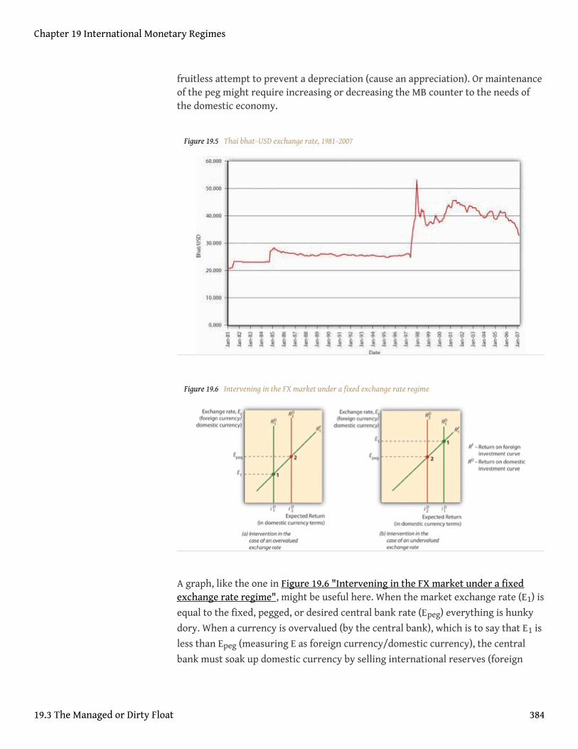
fruitless attempt to prevent a depreciation (cause an appreciation). Or maintenanceof the peg might require increasing or decreasing the MB counter to the needs ofthe domestic economy.
Figure 19.5 Thai bhat–USD exchange rate, 1981–2007
Figure 19.6 Intervening in the FX market under a fixed exchange rate regime
A graph, like the one in Figure 19.6 "Intervening in the FX market under a fixedexchange rate regime", might be useful here. When the market exchange rate (E1) is
equal to the fixed, pegged, or desired central bank rate (Epeg) everything is hunky
dory. When a currency is overvalued (by the central bank), which is to say that E1 is
less than Epeg (measuring E as foreign currency/domestic currency), the central
bank must soak up domestic currency by selling international reserves (foreign
Chapter 19 International Monetary Regimes
19.3 The Managed or Dirty Float 384
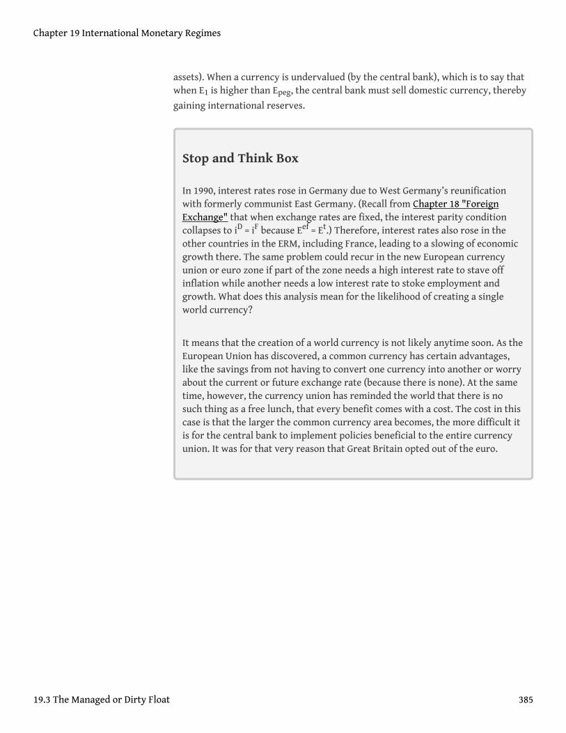
assets). When a currency is undervalued (by the central bank), which is to say thatwhen E1 is higher than Epeg, the central bank must sell domestic currency, thereby
gaining international reserves.
Stop and Think Box
In 1990, interest rates rose in Germany due to West Germany’s reunificationwith formerly communist East Germany. (Recall from Chapter 18 "ForeignExchange" that when exchange rates are fixed, the interest parity conditioncollapses to iD = iF because Eef = Et.) Therefore, interest rates also rose in theother countries in the ERM, including France, leading to a slowing of economicgrowth there. The same problem could recur in the new European currencyunion or euro zone if part of the zone needs a high interest rate to stave offinflation while another needs a low interest rate to stoke employment andgrowth. What does this analysis mean for the likelihood of creating a singleworld currency?
It means that the creation of a world currency is not likely anytime soon. As theEuropean Union has discovered, a common currency has certain advantages,like the savings from not having to convert one currency into another or worryabout the current or future exchange rate (because there is none). At the sametime, however, the currency union has reminded the world that there is nosuch thing as a free lunch, that every benefit comes with a cost. The cost in thiscase is that the larger the common currency area becomes, the more difficult itis for the central bank to implement policies beneficial to the entire currencyunion. It was for that very reason that Great Britain opted out of the euro.
Chapter 19 International Monetary Regimes
19.3 The Managed or Dirty Float 385
KEY TAKEAWAYS
• Central banks influence the FX rate via unsterilized foreign exchangeinterventions or, more specifically, by buying or selling internationalreserves (foreign assets) with domestic currency.
• When central banks buy international reserves, they increase MB andhence depreciate their respective currencies by increasing inflationexpectations.
• When central banks sell international reserves, they decrease MB andhence appreciate their respective currencies by decreasing inflationexpectations.
Chapter 19 International Monetary Regimes
19.3 The Managed or Dirty Float 386
19.4 The Choice of International Policy Regime
LEARNING OBJECTIVE
1. What are the costs and benefits of fixing the FX rate or keeping it withina narrow band?
Problems ensue when the central bank runs out of reserves, as it did in Thailand in 1997.The International Monetary Fund (IMF) often provides loans to countriesattempting to defend the value of their currencies. It doesn’t really act as aninternational lender of last resort, however, because it doesn’t follow Hamilton’snée Bagehot’s Law. It simply has no mechanism for adding liquidity quickly, and thelonger one waits, the bigger the eventual bill. Moreover, the IMF often forcesborrowers to undergo fiscal austerity programs (high government taxes, decreasedexpenditures, high domestic interest rates, and so forth) that can create as mucheconomic pain as a rapid depreciation would. Finally, it has created a major moralhazard problem, repeatedly lending to the same few countries, which quicklylearned that they need not engage in responsible policies in the long run becausethe IMF would be sure to help out if they got into trouble. Sometimes the medicineis indeed worse than the disease!
Trouble can also arise when a central bank no longer wants to accumulate internationalreserves (or indeed any assets) because it wants to squelch domestic inflation, as it did inGermany in 1990–1992. Many fear that China, which currently owns over $1 trillion ininternational reserves (mostly USD), will find itself in this conundrum soon. TheChinese government accumulated such a huge amount of reserves by fixing itscurrency (which confusingly goes by two names, the yuan and the renminbi, butone symbol, CNY) at the rate of CNY8.28 per USD. Due to the growth of the Chineseeconomy relative to the U.S. economy, E* exceeded Epeg, inducing the Chinese, per
the analysis above, to sell CNY for international reserves to keep the yuanpermanently weak, or undervalued relative to the value the market would haveassigned it.
You should recall from Chapter 18 "Foreign Exchange" that undervaluing the yuanhelps Chinese exports by making them appear cheap to foreigners. (If you don’tbelieve me, walk into any Wal-Mart, Target, or other discount store.) Many peoplethink that China’s peg is unfair, a monetary form of dirty pool. Such folks need to realizethat there is no such thing as a free lunch. To maintain its peg, the Chinesegovernment has severely restricted international capital mobility via currency
Chapter 19 International Monetary Regimes
387
controls, thereby injuring the efficiency of Chinese financial markets, limitingforeign direct investment, and encouraging mass loophole mining. It is also stuckwith a trillion bucks of relatively low-yielding international reserves that willdecline in value when the yuan floats (and probably appreciates strongly), as iteventually must. In other words, China is setting itself up for the exact opposite of theSoutheast Asian Crisis of 1997–1998, where the value of its assets will plummet instead of thevalue of its liabilities skyrocketing.
In China’s defense, many developing countries find it advantageous to peg theirexchange rates to the dollar, the yen, the euro, the pound sterling, or a basket ofsuch important currencies. The peg, which can be thought of as a monetary policy targetsimilar to an inflation or money supply target, allows the developing nation’s central bank tofigure out whether to increase or decrease MB and by how much. A hard peg or narrow bandeffectively ties the domestic inflation rate to that of the anchor country, As noted inChapter 18 "Foreign Exchange", however, not all goods and services are tradedinternationally, so the rates will not be exactly equal. instilling confidence in thedeveloping country’s macroeconomic performance.
Indeed, in extreme cases, some countries have given up their central bankaltogether and have dollarized, adopting USD or other currencies (though theprocess is still called dollarization) as their own. No international law prevents this,and indeed the country whose currency is adopted earns seigniorage and hence haslittle grounds for complaint. Countries that want to completely outsource theirmonetary policy but maintain seigniorage revenue (the profits from the issuance ofmoney) adopt a currency board that issues domestic currency but backs it 100percent with assets denominated in the anchor currency. (The board invests thereserves in interest-bearing assets, the source of the seigniorage.) Argentinabenefited from just such a board during the 1990s, when it pegged its peso one-to-one with the dollar, because it finally got inflation, which often ran over 100percent per year, under control.
Fixed exchange rates not based on commodities like gold or silver are notoriously fragile,however, because relative macroeconomic changes in interest rates, trade, and productivitycan create persistent imbalances over time between the developing and the anchorcurrencies. Moreover, speculators can force countries to devalue (move Epeg down)
or revalue (move Epeg up) when they hit the bottom or top of a band. They do so by
using the derivatives markets to place big bets on the future exchange rate. Unlikemost bets, these are one-sided because the speculators lose little money if thecentral bank successfully defends the peg, but they win a lot if it fails to. SpeculatorGeorge Soros, for example, is reported to have made $1 billion speculating againstthe pound sterling during the ERM balance of payments crisis in September 1992.Such crises can cause tremendous economic pain, as when Argentina found it
Chapter 19 International Monetary Regimes
19.4 The Choice of International Policy Regime 388
necessary to abandon its currency board and one-to-one peg with the dollar in2001–2002 due to speculative pressures and fundamental macroeconomicmisalignment between the Argentine and U.S. economies. (Basically, the UnitedStates was booming and Argentina was in a recession. The former needed higherinterest rates/slower money growth and the latter needed lower interest rates/higher money growth.)
Developing countries may be best off maintaining what is called a crawling target orcrawling peg. Generally, this entails the developing country’s central bank allowingits domestic currency to depreciate or appreciate over time, as generalmacroeconomic conditions (the variables discussed in Chapter 18 "ForeignExchange") dictate. A similar strategy is to recognize imbalances as they occur andchange the peg on an ad hoc basis accordingly, perhaps first by allowing the band towiden before permanently moving it. In those ways, developing countries canmaintain some FX rate stability, keep inflation in check (though perhaps higherthan in the anchor country), and hopefully avoid exchange rate crises.
Chapter 19 International Monetary Regimes
19.4 The Choice of International Policy Regime 389
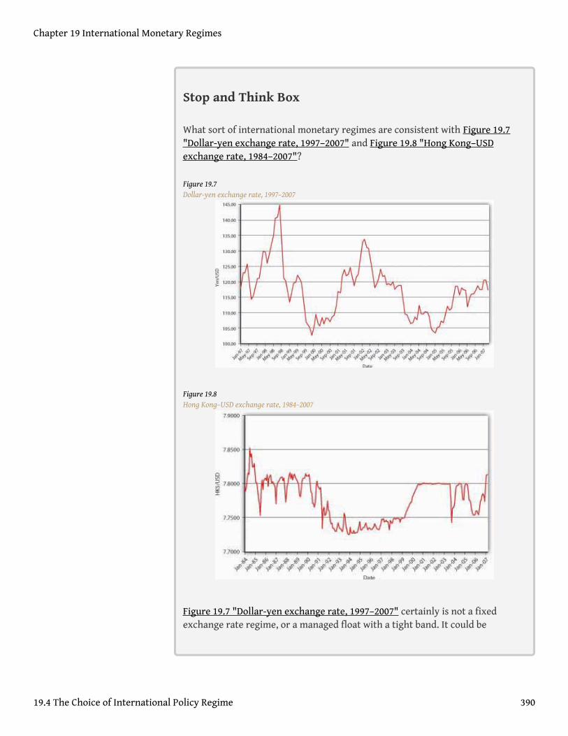
Stop and Think Box
What sort of international monetary regimes are consistent with Figure 19.7"Dollar-yen exchange rate, 1997–2007" and Figure 19.8 "Hong Kong–USDexchange rate, 1984–2007"?
Figure 19.7Dollar-yen exchange rate, 1997–2007
Figure 19.8Hong Kong–USD exchange rate, 1984–2007
Figure 19.7 "Dollar-yen exchange rate, 1997–2007" certainly is not a fixedexchange rate regime, or a managed float with a tight band. It could be
Chapter 19 International Monetary Regimes
19.4 The Choice of International Policy Regime 390
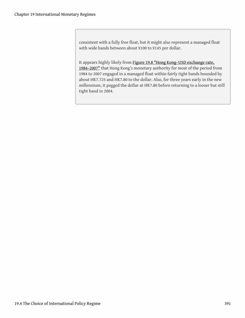
consistent with a fully free float, but it might also represent a managed floatwith wide bands between about ¥100 to ¥145 per dollar.
It appears highly likely from Figure 19.8 "Hong Kong–USD exchange rate,1984–2007" that Hong Kong’s monetary authority for most of the period from1984 to 2007 engaged in a managed float within fairly tight bands bounded byabout HK7.725 and HK7.80 to the dollar. Also, for three years early in the newmillennium, it pegged the dollar at HK7.80 before returning to a looser but stilltight band in 2004.
Chapter 19 International Monetary Regimes
19.4 The Choice of International Policy Regime 391
KEY TAKEAWAYS
• A country with weak institutions (e.g., a dependent central bank thatallows rampant inflation) can essentially free-ride on the monetarypolicy of a developed country by fixing or pegging its currency to thedollar, euro, yen, pound sterling, or other anchoring currency to agreater or lesser degree.
• In fact, in the limit, a country can simply adopt another country’scurrency as its own in a process called dollarization.
• If it wants to continue earning seigniorage (profits from the issuance ofmoney), it can create a currency board, the function of which is tomaintain 100 percent reserves and full convertibility between thedomestic currency and the anchor currency.
• At the other extreme, it can create a crawling peg with wide bands,allowing its currency to appreciate or depreciate day to day according tothe interaction of supply and demand, slowly adjusting the band and pegin the long term as macroeconomic conditions dictate.
• When a currency is overvalued, which is to say, when the central banksets Epeg higher than E* (when E is expressed as foreign currency/domestic currency), the central bank must appreciate the currency byselling international reserves for its domestic currency.
• It may run out of reserves before doing so, however, sparking a rapiddepreciation that could trigger a financial crisis by rapidly increasingthe real value of debts owed by domestic residents but denominated inforeign currencies.
• When a currency is undervalued, which is to say, when the central banksets Epeg below E*, the central bank must depreciate its domesticcurrency by exchanging it for international reserves. It may accumulatetoo many such reserves, which often have low yields and which couldquickly lose value if the domestic currency suddenly appreciates,perhaps with the aid of a good push by currency speculators making bigone-sided bets.
Chapter 19 International Monetary Regimes
19.4 The Choice of International Policy Regime 392
19.5 Suggested Reading
Bordon, Michael, and Barry Eichengreen. A Retrospective on the Bretton WoodsSystemml: Lessons for International Monetary Reform. Chicago, IL: University of ChicagoPress, 1993.
Eichengreen, Barry. Globalizing Capital: A History of the International Monetary System.Princeton, NJ: Princeton University Press, 2008.
Gallorotti, Giulio. The Anatomy of an International Monetary Regime: The Classical GoldStandard, 1880–1914. New York: Oxford University Press, 1995.
Moosa, Imad. Exchange Rate Regimes: Fixed, Flexible or Something in Between. New York:Palgrave Macmillan, 2005.
Rosenberg, Michael. Exchange Rate Determination: Models and Strategies for ExchangeRate Forecasting. New York: McGraw-Hill, 2003.
Chapter 19 International Monetary Regimes
393
Chapter 20
Money Demand
CHAPTER OBJECTIVES
By the end of this chapter, students should be able to:
1. Describe Friedman’s modern quantity theory of money.2. Describe the classical quantity theory.3. Describe Keynes’s liquidity preference theory and its improvements.4. Contrast the modern quantity theory with the liquidity preference
theory.
394
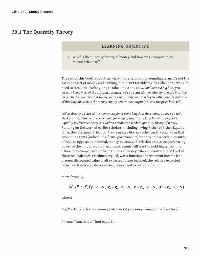
20.1 The Quantity Theory
LEARNING OBJECTIVE
1. What is the quantity theory of money and how was it improved byMilton Friedman?
The rest of this book is about monetary theory, a daunting-sounding term. It’s not theeasiest aspect of money and banking, but it isn’t terribly taxing either so there is noneed to freak out. We’re going to take it nice and slow. And here’s a big hint: youalready know most of the outcomes because we’ve discussed them already in more intuitiveterms. In the chapters that follow, we’re simply going to provide you with more formal waysof thinking about how the money supply determines output (Y*) and the price level (P*).
We’ve already discussed the money supply at some length in the chapters above, so we’llstart our theorizing with the demand for money, specifically John Maynard Keynes’sliquidity preference theory and Milton Friedman’s modern quantity theory of money.Building on the work of earlier scholars, including Irving Fisher of Fisher Equationfame, the late, great Friedman treats money like any other asset, concluding thateconomic agents (individuals, firms, governments) want to hold a certain quantityof real, as opposed to nominal, money balances. If inflation erodes the purchasingpower of the unit of account, economic agents will want to hold higher nominalbalances to compensate, to keep their real money balances constant. The level ofthose real balances, Friedman argued, was a function of permanent income (thepresent discounted value of all expected future income), the relative expectedreturn on bonds and stocks versus money, and expected inflation.
More formally,
where:
Md/P = demand for real money balances (Md = money demand; P = price level)
f means “function of” (not equal to)
Md /P : f (Yp <+>, rb– rm <−>, rs– rm <−>, πe– rm <−>)
Chapter 20 Money Demand
395
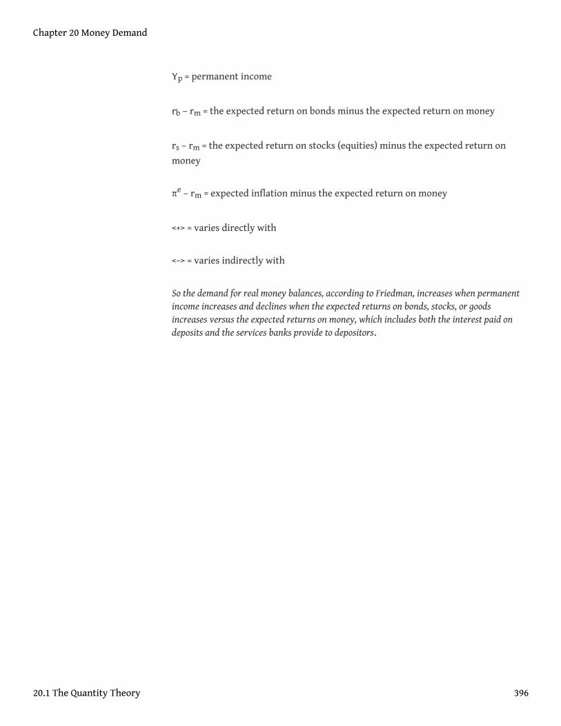
Yp = permanent income
rb – rm = the expected return on bonds minus the expected return on money
rs – rm = the expected return on stocks (equities) minus the expected return on
money
πe – rm = expected inflation minus the expected return on money
<+> = varies directly with
<−> = varies indirectly with
So the demand for real money balances, according to Friedman, increases when permanentincome increases and declines when the expected returns on bonds, stocks, or goodsincreases versus the expected returns on money, which includes both the interest paid ondeposits and the services banks provide to depositors.
Chapter 20 Money Demand
20.1 The Quantity Theory 396
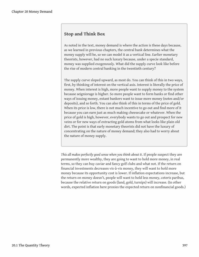
Stop and Think Box
As noted in the text, money demand is where the action is these days because,as we learned in previous chapters, the central bank determines what themoney supply will be, so we can model it as a vertical line. Earlier monetarytheorists, however, had no such luxury because, under a specie standard,money was supplied exogenously. What did the supply curve look like beforethe rise of modern central banking in the twentieth century?
The supply curve sloped upward, as most do. You can think of this in two ways,first, by thinking of interest on the vertical axis. Interest is literally the price ofmoney. When interest is high, more people want to supply money to the systembecause seigniorage is higher. So more people want to form banks or find otherways of issuing money, extant bankers want to issue more money (notes and/ordeposits), and so forth. You can also think of this in terms of the price of gold.When its price is low, there is not much incentive to go out and find more of itbecause you can earn just as much making cheesecake or whatever. When theprice of gold is high, however, everybody wants to go out and prospect for newveins or for new ways of extracting gold atoms from what looks like plain olddirt. The point is that early monetary theorists did not have the luxury ofconcentrating on the nature of money demand; they also had to worry aboutthe nature of money supply.
This all makes perfectly good sense when you think about it. If people suspect they arepermanently more wealthy, they are going to want to hold more money, in realterms, so they can buy caviar and fancy golf clubs and what not. If the return onfinancial investments decreases vis-à-vis money, they will want to hold moremoney because its opportunity cost is lower. If inflation expectations increase, butthe return on money doesn’t, people will want to hold less money, ceteris paribus,because the relative return on goods (land, gold, turnips) will increase. (In otherwords, expected inflation here proxies the expected return on nonfinancial goods.)
Chapter 20 Money Demand
20.1 The Quantity Theory 397
KEY TAKEAWAYS
• According to Milton Friedman, demand for real money balances (Md/P)is directly related to permanent income (Yp)—the discounted presentvalue of expected future income—and indirectly related to the expecteddifferential returns from bonds, stocks (equities), and goods vis-à-vismoney (rb – rm, rs – rm, πe – rm ), where inflation (π) proxies the returnon goods.
• Because he believed that the return on money would increase (decrease)as returns on bonds, stocks, and goods increased (decreased), Friedmandid not think that interest rate changes mattered much.
Chapter 20 Money Demand
20.1 The Quantity Theory 398
20.2 Liquidity Preference Theory
LEARNING OBJECTIVE
1. What is the liquidity preference theory and how has it been improved?
The very late and very great John Maynard Keynes (to distinguish him from hisfather, economist John Neville Keynes) developed the liquidity preference theory inresponse to the rather primitive pre-Friedman quantity theory of money, which wassimply an assumption-laden identity called the equation of exchange:
where:
M = money supply
V = velocity
P = price level
Y = output
Nobody doubted the equation itself, which, as an identity (like x = x), is undeniable.But many doubted the way that classical quantity theorists used the equation of exchange asthe causal statement: increases in the money supply lead to proportional increases in theprice level. The classical quantity theory also suffered by assuming that money velocity, thenumber of times per year a unit of currency was spent, was constant. Although a goodfirst approximation of reality, the classical quantity theory, which critics derided asthe “naïve quantity theory of money,” was hardly the entire story. In particular, itcould not explain why velocity was pro-cyclical, i.e., why it increased duringbusiness expansions and decreased during recessions.
To find a better theory, Keynes took a different point of departure, asking in effect,“Why do economic agents hold money?” He came up with three reasons:
MV = PY
Chapter 20 Money Demand
399
1. Transactions: Economic agents need money to make payments. Astheir incomes rise, so, too, do the number and value of those payments,so this part of money demand is proportional to income.
2. Precautions: S—t happens was a catch phrase of the 1980s, recalledperhaps most famously in the hit movie Forrest Gump. Way back in the1930s, Keynes already knew that bad stuff happens—and that onedefense against it was to keep some spare cash lying around as aprecaution. It, too, is directly proportional to income, Keynes believed.
3. Speculations: People will hold more bonds than money when interestrates are high for two reasons. The opportunity cost of holding money(which Keynes assumed has zero return) is higher and the expectationis that interest rates will fall, raising the price of bonds. When interestrates are low, the opportunity cost of holding money is low, and theexpectation is that rates will rise, decreasing the price of bonds. Sopeople hold larger money balances when rates are low. Overall, then,money demand and interest rates are inversely related.
More formally, Keynes’s ideas can be stated as
where:
Md/P = demand for real money balances
f means “function of” (this simplifies the mathematics)
i = interest rate
Y = output (income)
<+> = varies directly with
<−> = varies indirectly with
An increase in interest rates induces people to decrease real money balances for agiven income level, implying that velocity must be higher. So Keynes’s view wassuperior to the classical quantity theory of money because he showed that velocity is notconstant but rather is positively related to interest rates, thereby explaining its pro-cyclicalnature. (Recall from Chapter 5 "The Economics of Interest-Rate Fluctuations" that
Md /P = f (i <−>, Y <+>)
Chapter 20 Money Demand
20.2 Liquidity Preference Theory 400
interest rates rise during expansions and fall during recessions.) Keynes’s theory wasalso fruitful because it induced other scholars to elaborate on it further.
In the early 1950s, for example, a young WillBaumolhttp://pages.stern.nyu.edu/~wbaumol/ and JamesTobinhttp://nobelprize.org/nobel_prizes/economics/laureates/1981/tobin-autobio.html independently showed that money balances, held for transactionpurposes (not just speculative ones), were sensitive to interest rates, even if the returnon money was zero. That is because people can hold bonds or other interest-bearingsecurities until they need to make a payment. When interest rates are high, peoplewill hold as little money for transaction purposes as possible because it will beworth the time and trouble of investing in bonds and then liquidating them whenneeded. When rates are low, by contrast, people will hold more money fortransaction purposes because it isn’t worth the hassle and brokerage fees to playwith bonds very often. So transaction demand for money is negatively related to interestrates. A similar trade-off applies also to precautionary balances. The lure of highinterest rates offsets the fear of bad events occurring. When rates are low, better toplay it safe and hold more dough. So the precautionary demand for money is alsonegatively related to interest rates.
Chapter 20 Money Demand
20.2 Liquidity Preference Theory 401
KEY TAKEAWAYS
• Before Friedman, the quantity theory of money was a much simpleraffair based on the so-called equation of exchange—money timesvelocity equals the price level times output (MV = PY)—plus theassumptions that changes in the money supply cause changes in outputand prices and that velocity changes so slowly it can be safely treated asa constant. Note that the interest rate is not considered at all in this so-called naïve version.
• Keynes and his followers knew that interest rates were important tomoney demand and that velocity wasn’t a constant, so they created atheory whereby economic actors demand money to engage intransactions (buy and sell goods), as a precaution against unexpectednegative shocks, and as a speculation.
• Due to the first two motivations, real money balances increase directlywith output.
• Due to the speculative motive, real money balances and interest ratesare inversely related. When interest rates are high, so is the opportunitycost of holding money.
• Throw in the expectation that rates will likely fall, causing bond pricesto rise, and people are induced to hold less money and more bonds.
• When interest rates are low, by contrast, people expect them to rise,which will hurt bond prices. Moreover, the opportunity cost of holdingmoney to make transactions or as a precaution against shocks is lowwhen interest rates are low, so people will hold more money and fewerbonds when interest rates are low.
Chapter 20 Money Demand
20.2 Liquidity Preference Theory 402
20.3 Head to Head: Friedman versus Keynes
LEARNING OBJECTIVE
1. How do the modern quantity theory and the liquidity preference theorycompare?
Friedman’s elaboration of the quantity theory drew heavily on Keynes’s and his followers’insights as well, so it is not surprising that Friedman’s view eventually predominated. Themodern quantity theory is superior to Keynes’s liquidity preference theory becauseit is more complex, specifying three types of assets (bonds, equities, goods) insteadof just one (bonds). It also does not assume that the return on money is zero, oreven a constant. In Friedman’s theory, velocity is no longer a constant; instead, it ishighly predictable and, as in reality and Keynes’s formulation, pro-cyclical, risingduring expansions and falling during recessions.
Finally, unlike the liquidity preference theory, Friedman’s modern quantity theory predictsthat interest rate changes should have little effect on money demand. The reason for thisis that Friedman believed that the return on bonds, stocks, goods, and money wouldbe positively correlated, leading to little change in rb – rm, rs – rm, or πe – rm
because both sides would rise or fall about the same amount. That insightessentially reduces the modern quantity theory to Md/P = f(Yp <+>). Until the 1970s,
Friedman was more or less correct. Interest rates did not strongly affect the demandfor money, so velocity was predictable and the quantity of money was closely linkedto aggregate output. Except when nominal interest rates hit zero (as in Japan), thedemand for money was somewhat sensitive to interest rates, so there was no so-called liquidity trap (where money demand is perfectly horizontal, leaving centralbankers impotent). During the 1970s, however, money demand became more sensitive tointerest rate changes, and velocity, output, and inflation became harder to predict. That’sone reason, noted in Chapter 17 "Monetary Policy Targets and Goals", why centralbanks in the 1970s found that targeting monetary aggregates did not help them tomeet their inflation or output goals.
Chapter 20 Money Demand
403
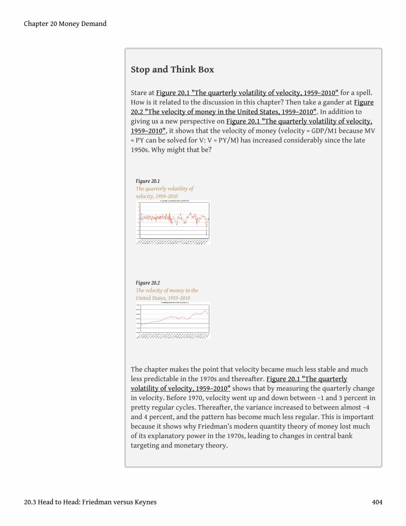
Stop and Think Box
Stare at Figure 20.1 "The quarterly volatility of velocity, 1959–2010" for a spell.How is it related to the discussion in this chapter? Then take a gander at Figure20.2 "The velocity of money in the United States, 1959–2010". In addition togiving us a new perspective on Figure 20.1 "The quarterly volatility of velocity,1959–2010", it shows that the velocity of money (velocity = GDP/M1 because MV= PY can be solved for V: V = PY/M) has increased considerably since the late1950s. Why might that be?
Figure 20.1The quarterly volatility ofvelocity, 1959–2010
Figure 20.2The velocity of money in theUnited States, 1959–2010
The chapter makes the point that velocity became much less stable and muchless predictable in the 1970s and thereafter. Figure 20.1 "The quarterlyvolatility of velocity, 1959–2010" shows that by measuring the quarterly changein velocity. Before 1970, velocity went up and down between −1 and 3 percent inpretty regular cycles. Thereafter, the variance increased to between almost −4and 4 percent, and the pattern has become much less regular. This is importantbecause it shows why Friedman’s modern quantity theory of money lost muchof its explanatory power in the 1970s, leading to changes in central banktargeting and monetary theory.
Chapter 20 Money Demand
20.3 Head to Head: Friedman versus Keynes 404
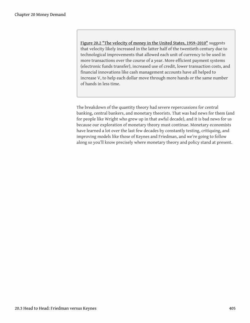
Figure 20.2 "The velocity of money in the United States, 1959–2010" suggeststhat velocity likely increased in the latter half of the twentieth century due totechnological improvements that allowed each unit of currency to be used inmore transactions over the course of a year. More efficient payment systems(electronic funds transfer), increased use of credit, lower transaction costs, andfinancial innovations like cash management accounts have all helped toincrease V, to help each dollar move through more hands or the same numberof hands in less time.
The breakdown of the quantity theory had severe repercussions for centralbanking, central bankers, and monetary theorists. That was bad news for them (andfor people like Wright who grew up in that awful decade), and it is bad news for usbecause our exploration of monetary theory must continue. Monetary economistshave learned a lot over the last few decades by constantly testing, critiquing, andimproving models like those of Keynes and Friedman, and we’re going to followalong so you’ll know precisely where monetary theory and policy stand at present.
Chapter 20 Money Demand
20.3 Head to Head: Friedman versus Keynes 405
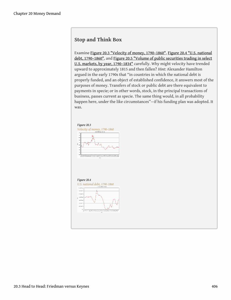
Stop and Think Box
Examine Figure 20.3 "Velocity of money, 1790–1860", Figure 20.4 "U.S. nationaldebt, 1790–1860", and Figure 20.5 "Volume of public securities trading in selectU.S. markets, by year, 1790–1834" carefully. Why might velocity have trendedupward to approximately 1815 and then fallen? Hint: Alexander Hamiltonargued in the early 1790s that “in countries in which the national debt isproperly funded, and an object of established confidence, it answers most of thepurposes of money. Transfers of stock or public debt are there equivalent topayments in specie; or in other words, stock, in the principal transactions ofbusiness, passes current as specie. The same thing would, in all probabilityhappen here, under the like circumstances”—if his funding plan was adopted. Itwas.
Figure 20.3Velocity of money, 1790–1860
Figure 20.4U.S. national debt, 1790–1860
Chapter 20 Money Demand
20.3 Head to Head: Friedman versus Keynes 406
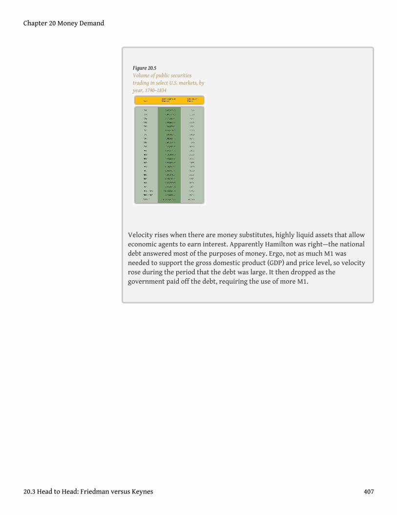
Figure 20.5Volume of public securitiestrading in select U.S. markets, byyear, 1790–1834
Velocity rises when there are money substitutes, highly liquid assets that alloweconomic agents to earn interest. Apparently Hamilton was right—the nationaldebt answered most of the purposes of money. Ergo, not as much M1 wasneeded to support the gross domestic product (GDP) and price level, so velocityrose during the period that the debt was large. It then dropped as thegovernment paid off the debt, requiring the use of more M1.
Chapter 20 Money Demand
20.3 Head to Head: Friedman versus Keynes 407
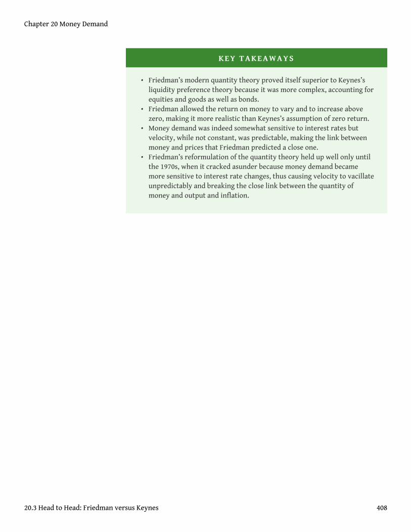
KEY TAKEAWAYS
• Friedman’s modern quantity theory proved itself superior to Keynes’sliquidity preference theory because it was more complex, accounting forequities and goods as well as bonds.
• Friedman allowed the return on money to vary and to increase abovezero, making it more realistic than Keynes’s assumption of zero return.
• Money demand was indeed somewhat sensitive to interest rates butvelocity, while not constant, was predictable, making the link betweenmoney and prices that Friedman predicted a close one.
• Friedman’s reformulation of the quantity theory held up well only untilthe 1970s, when it cracked asunder because money demand becamemore sensitive to interest rate changes, thus causing velocity to vacillateunpredictably and breaking the close link between the quantity ofmoney and output and inflation.
Chapter 20 Money Demand
20.3 Head to Head: Friedman versus Keynes 408
20.4 Suggested Reading
Friedman, Milton. Money Mischief: Episodes in Monetary History. New York: Harvest,1994.
Friedman, Milton, and Anna Jacobson. A Monetary History of the United States,1867–1960 (Princeton, NJ: Princeton University Press, 1971).
Kindleberger, Charles. Keynesianism vs. Monetarism and Other Essays in FinancialHistory. London: George Allen & Unwin, 1985.
Minsky, Hyman. John Maynard Keynes. New York: McGraw-Hill, 2008)
Serletis, Apostolos. The Demand for Money: Theoretical and Empirical Approaches. NewYork: Springer, 2007.
Chapter 20 Money Demand
409
Chapter 21
IS-LM
CHAPTER OBJECTIVES
By the end of this chapter, students should be able to:
1. Explain this equation: Y = Yad = C + I + G + NX.2. Provide the equation for C and explain its importance.3. Describe the Keynesian cross diagram and explain its use.4. Describe the investment-savings (IS) curve and its characteristics.5. Describe the liquidity preference–money (LM) curve and its
characteristics.6. Explain why equilibrium is achieved in the markets for goods and
money.7. Explain the IS-LM model’s biggest drawback.
410
21.1 Aggregate Output and Keynesian Cross Diagrams
LEARNING OBJECTIVES
1. What does this equation mean: Y = Yad = C + I + G + NX?2. Why is this equation important?3. What is the equation for C and why is it important?4. What is the Keynesian cross diagram and what does it help us to do?
Developed in 1937 by economist and Keynes disciple John Hicks, the IS-LM model is still usedtoday to model aggregate output (gross domestic product [GDP], gross national product[GNP], etc.) and interest rates in the short run.http://en.wikipedia.org/wiki/John_HicksIt begins with John Maynard Keynes’s recognition that
where:
Y = aggregate output (supplied)
Yad = aggregate demand
C = consumer expenditure
I = investment (on new physical capital like computers and factories, and plannedinventory)
G = government spending
NX = net exports (exports minus imports)
Keynes further explained that C = a + (mpc × Yd)
where:
Y = Y ad = C + I + G + NX
Chapter 21 IS-LM
411
Yd = disposable income, all that income above a
a = autonomous consumer expenditure (food, clothing, shelter, and othernecessaries)
mpc = marginal propensity to consume (change in consumer expenditure from anextra dollar of income or “disposable income;” it is a constant bounded by 0 and 1)
Practice calculating C in Exercise 1.
Chapter 21 IS-LM
21.1 Aggregate Output and Keynesian Cross Diagrams 412
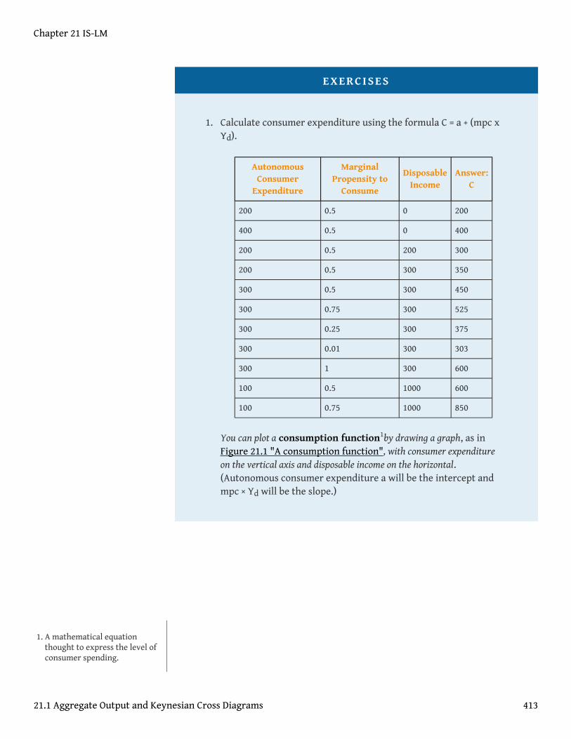
EXERCISES
1. Calculate consumer expenditure using the formula C = a + (mpc xYd).
AutonomousConsumer
Expenditure
MarginalPropensity to
Consume
DisposableIncome
Answer:C
200 0.5 0 200
400 0.5 0 400
200 0.5 200 300
200 0.5 300 350
300 0.5 300 450
300 0.75 300 525
300 0.25 300 375
300 0.01 300 303
300 1 300 600
100 0.5 1000 600
100 0.75 1000 850
You can plot a consumption function1by drawing a graph, as inFigure 21.1 "A consumption function", with consumer expenditureon the vertical axis and disposable income on the horizontal.(Autonomous consumer expenditure a will be the intercept andmpc × Yd will be the slope.)
1. A mathematical equationthought to express the level ofconsumer spending.
Chapter 21 IS-LM
21.1 Aggregate Output and Keynesian Cross Diagrams 413
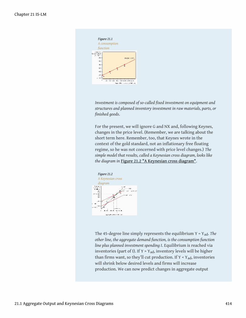
Figure 21.1A consumptionfunction
Investment is composed of so-called fixed investment on equipment andstructures and planned inventory investment in raw materials, parts, orfinished goods.
For the present, we will ignore G and NX and, following Keynes,changes in the price level. (Remember, we are talking about theshort term here. Remember, too, that Keynes wrote in thecontext of the gold standard, not an inflationary free floatingregime, so he was not concerned with price level changes.) Thesimple model that results, called a Keynesian cross diagram, looks likethe diagram in Figure 21.2 "A Keynesian cross diagram".
Figure 21.2A Keynesian crossdiagram
The 45-degree line simply represents the equilibrium Y = Yad. Theother line, the aggregate demand function, is the consumption functionline plus planned investment spending I. Equilibrium is reached viainventories (part of I). If Y > Yad, inventory levels will be higherthan firms want, so they’ll cut production. If Y < Yad, inventorieswill shrink below desired levels and firms will increaseproduction. We can now predict changes in aggregate output
Chapter 21 IS-LM
21.1 Aggregate Output and Keynesian Cross Diagrams 414
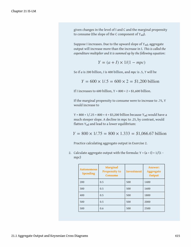
given changes in the level of I and C and the marginal propensityto consume (the slope of the C component of Yad).
Suppose I increases. Due to the upward slope of Yad, aggregateoutput will increase more than the increase in I. This is called theexpenditure multiplier and it is summed up by the following equation:
So if a is 200 billion, I is 400 billion, and mpc is .5, Y will be
If I increases to 600 billion, Y = 800 × 2 = $1,600 billion.
If the marginal propensity to consume were to increase to .75, Ywould increase to
Y = 800 × 1/.25 = 800 × 4 = $3,200 billion because Yad would have amuch steeper slope. A decline in mpc to .25, by contrast, wouldflatten Yad and lead to a lower equilibrium:
Practice calculating aggregate output in Exercise 2.
2. Calculate aggregate output with the formula: Y = (a + I) × 1/(1 −mpc)
AutonomousSpending
MarginalPropensity to
ConsumeInvestment
Answer:Aggregate
Output
200 0.5 500 1400
300 0.5 500 1600
400 0.5 500 1800
500 0.5 500 2000
500 0.6 500 2500
Y = (a + I) × 1/(1 − mpc)
Y = 600 × 1/.5 = 600 × 2 = $1,200 billion
Y = 800 × 1/.75 = 800 × 1.333 = $1,066.67 billion
Chapter 21 IS-LM
21.1 Aggregate Output and Keynesian Cross Diagrams 415
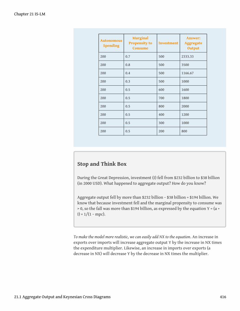
AutonomousSpending
MarginalPropensity to
ConsumeInvestment
Answer:Aggregate
Output
200 0.7 500 2333.33
200 0.8 500 3500
200 0.4 500 1166.67
200 0.3 500 1000
200 0.5 600 1600
200 0.5 700 1800
200 0.5 800 2000
200 0.5 400 1200
200 0.5 300 1000
200 0.5 200 800
Stop and Think Box
During the Great Depression, investment (I) fell from $232 billion to $38 billion(in 2000 USD). What happened to aggregate output? How do you know?
Aggregate output fell by more than $232 billion − $38 billion = $194 billion. Weknow that because investment fell and the marginal propensity to consume was> 0, so the fall was more than $194 billion, as expressed by the equation Y = (a +I) × 1/(1 − mpc).
To make the model more realistic, we can easily add NX to the equation. An increase inexports over imports will increase aggregate output Y by the increase in NX timesthe expenditure multiplier. Likewise, an increase in imports over exports (adecrease in NX) will decrease Y by the decrease in NX times the multiplier.
Chapter 21 IS-LM
21.1 Aggregate Output and Keynesian Cross Diagrams 416
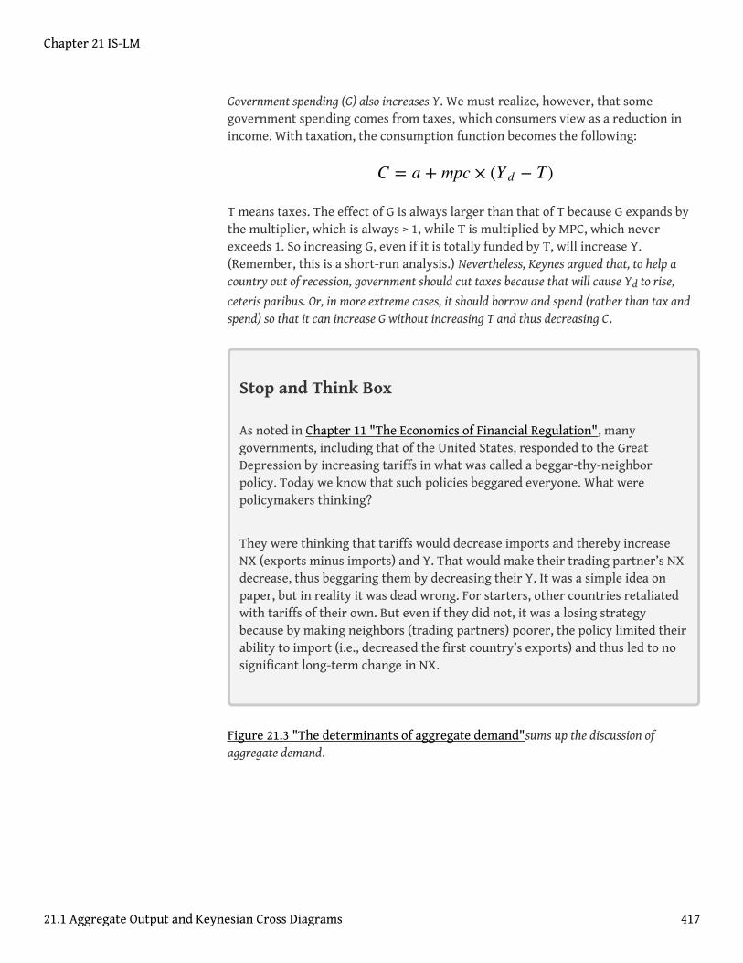
Government spending (G) also increases Y. We must realize, however, that somegovernment spending comes from taxes, which consumers view as a reduction inincome. With taxation, the consumption function becomes the following:
T means taxes. The effect of G is always larger than that of T because G expands bythe multiplier, which is always > 1, while T is multiplied by MPC, which neverexceeds 1. So increasing G, even if it is totally funded by T, will increase Y.(Remember, this is a short-run analysis.) Nevertheless, Keynes argued that, to help acountry out of recession, government should cut taxes because that will cause Yd to rise,
ceteris paribus. Or, in more extreme cases, it should borrow and spend (rather than tax andspend) so that it can increase G without increasing T and thus decreasing C.
Stop and Think Box
As noted in Chapter 11 "The Economics of Financial Regulation", manygovernments, including that of the United States, responded to the GreatDepression by increasing tariffs in what was called a beggar-thy-neighborpolicy. Today we know that such policies beggared everyone. What werepolicymakers thinking?
They were thinking that tariffs would decrease imports and thereby increaseNX (exports minus imports) and Y. That would make their trading partner’s NXdecrease, thus beggaring them by decreasing their Y. It was a simple idea onpaper, but in reality it was dead wrong. For starters, other countries retaliatedwith tariffs of their own. But even if they did not, it was a losing strategybecause by making neighbors (trading partners) poorer, the policy limited theirability to import (i.e., decreased the first country’s exports) and thus led to nosignificant long-term change in NX.
Figure 21.3 "The determinants of aggregate demand"sums up the discussion ofaggregate demand.
C = a + mpc × (Y d − T)
Chapter 21 IS-LM
21.1 Aggregate Output and Keynesian Cross Diagrams 417
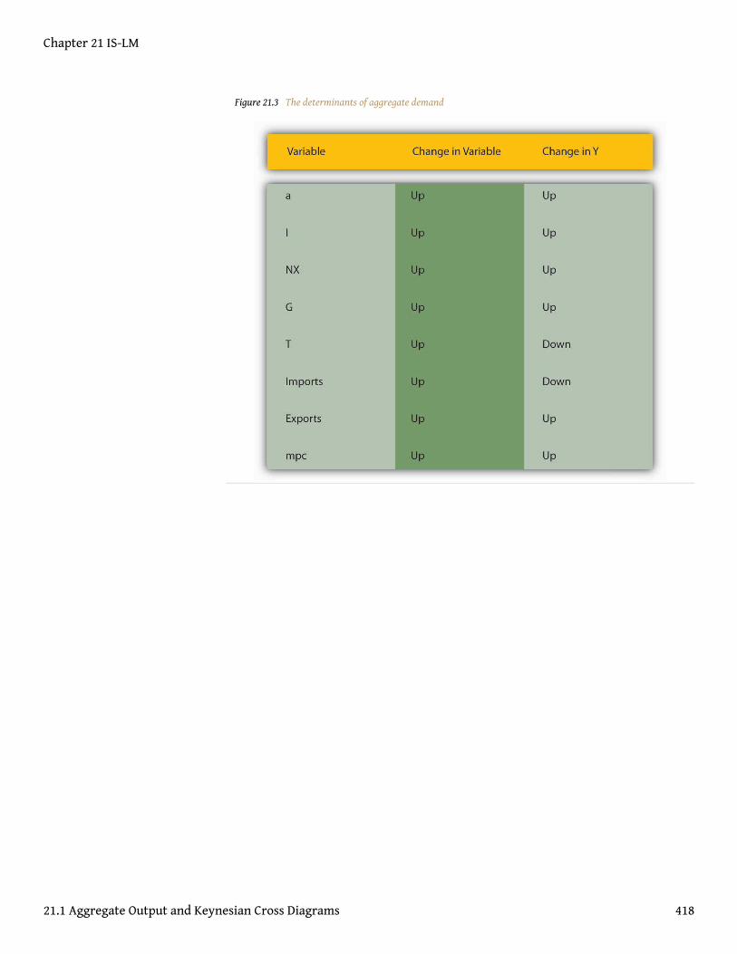
Figure 21.3 The determinants of aggregate demand
Chapter 21 IS-LM
21.1 Aggregate Output and Keynesian Cross Diagrams 418
KEY TAKEAWAYS
• The equation Y = Yad = C + I + G + NX tells us that aggregate output (oraggregate income) is equal to aggregate demand, which in turn is equalto consumer expenditure plus investment (planned, physical stuff) plusgovernment spending plus net exports (exports – imports).
• It is important because it allows economists to model aggregate output(to discern why, for example, GDP changes).
• In a taxless Eden, like the Gulf Cooperation Council countries, consumerexpenditure equals autonomous consumer expenditure (spending onnecessaries) (a) plus the marginal propensity to consume (mpc) timesdisposable income (Yd), income above a.
• In the rest of the world, C = a + mpc × (Yd − T), where T = taxes.• C, particularly the marginal propensity to consume variable, is
important because it gives the aggregate demand curve in a Keynesiancross diagram its upward slope.
• A Keynesian cross diagram is a graph with aggregate demand (Yad) onthe vertical axis and aggregate output (Y) on the horizontal.
• It consists of a 45-degree line where Y = Yad and a Yad curve, which plotsC + I + G + NX with the slope given by the expenditure multiplier, whichis the reciprocal of 1 minus the marginal propensity to consume: Y = (a +I + NX + G) × 1/(1 − mpc).
• The diagram helps us to see that aggregate output is directly related toa, I, exports, G, and mpc and indirectly related to T and imports.
Chapter 21 IS-LM
21.1 Aggregate Output and Keynesian Cross Diagrams 419
21.2 The IS-LM Model
LEARNING OBJECTIVES
1. What are the IS and LM curves?2. What are their characteristics?3. What do we learn when we combine the IS and the LM curves on one
graph?4. Why is equilibrium achieved?5. What is the IS-LM model’s biggest drawback?
The Keynesian cross diagram framework is great, as far as it goes. Note that it has nothingto say about interest rates or money, a major shortcoming for us students of money,banking, and monetary policy! It does, however, help us to build a more powerfulmodel that examines equilibrium in the markets for goods and money, the IS(investment-savings) and the LM (liquidity preference–money) curves, respectively(hence the name of the model).
Interest rates are negatively related to I and to NX. The reasoning here isstraightforward. When interest rates (i) are high, companies would rather invest inbonds than in physical plant (because fewer projects are positive net presentvalue2 or +NPV3) or inventory (because it has a high opportunity cost), so I(investment) is low. When rates are low, new physical plant and inventories lookcheap and many more projects are +NPV (i has come down in the denominator ofthe present value formula), so I is high. Similarly, when i is low, as we learned inChapter 18 "Foreign Exchange", the domestic currency will be weak, all else equal.Exports will be facilitated and imports will decline because foreign goods will lookexpensive. Thus, NX will be high (exports > imports). When i is high, by contrast,the domestic currency will be in demand and hence strong. That will hurt exportsand increase imports, so NX will drop and perhaps become negative (exports <imports).
Now think of Yad on a Keynesian cross diagram. As we saw above, aggregate output
will rise as I and NX do. So we know that as i increases, Yad decreases, ceteris
paribus. Plotting the interest rate on the vertical axis against aggregate output on thehorizontal axis, as below, gives us a downward sloping curve. That’s the IS curve! For eachinterest rate, it tells us at what point the market for goods (I and NX, get it?) is inequilibrium. For all points to the right of the curve, there is an excess supply ofgoods for that interest rate, which causes firms to decrease inventories, leading to a
2. A project likely to be profitableat a given interest rate aftercomparing the present valuesof both expenditures andrevenues. This will make moresense after you navigateChapter 4 "Interest Rates".
3. See positive net present value.
Chapter 21 IS-LM
420
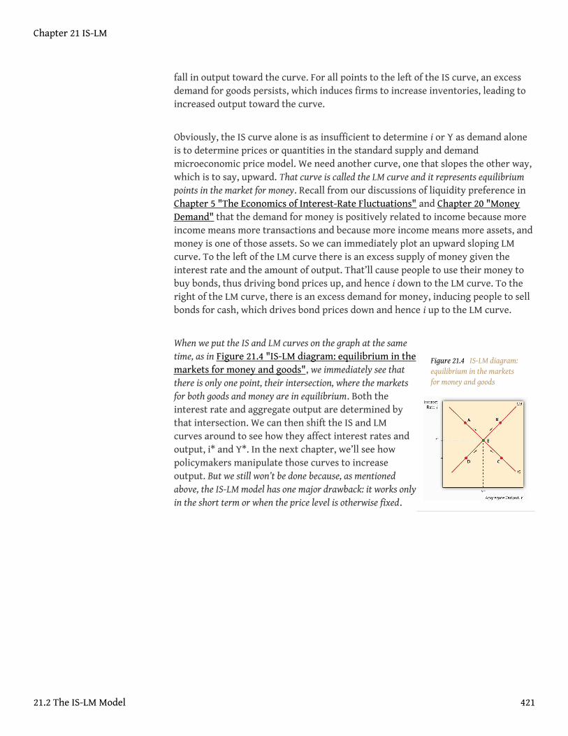
Figure 21.4 IS-LM diagram:equilibrium in the marketsfor money and goods
fall in output toward the curve. For all points to the left of the IS curve, an excessdemand for goods persists, which induces firms to increase inventories, leading toincreased output toward the curve.
Obviously, the IS curve alone is as insufficient to determine i or Y as demand aloneis to determine prices or quantities in the standard supply and demandmicroeconomic price model. We need another curve, one that slopes the other way,which is to say, upward. That curve is called the LM curve and it represents equilibriumpoints in the market for money. Recall from our discussions of liquidity preference inChapter 5 "The Economics of Interest-Rate Fluctuations" and Chapter 20 "MoneyDemand" that the demand for money is positively related to income because moreincome means more transactions and because more income means more assets, andmoney is one of those assets. So we can immediately plot an upward sloping LMcurve. To the left of the LM curve there is an excess supply of money given theinterest rate and the amount of output. That’ll cause people to use their money tobuy bonds, thus driving bond prices up, and hence i down to the LM curve. To theright of the LM curve, there is an excess demand for money, inducing people to sellbonds for cash, which drives bond prices down and hence i up to the LM curve.
When we put the IS and LM curves on the graph at the sametime, as in Figure 21.4 "IS-LM diagram: equilibrium in themarkets for money and goods", we immediately see thatthere is only one point, their intersection, where the marketsfor both goods and money are in equilibrium. Both theinterest rate and aggregate output are determined bythat intersection. We can then shift the IS and LMcurves around to see how they affect interest rates andoutput, i* and Y*. In the next chapter, we’ll see howpolicymakers manipulate those curves to increaseoutput. But we still won’t be done because, as mentionedabove, the IS-LM model has one major drawback: it works onlyin the short term or when the price level is otherwise fixed.
Chapter 21 IS-LM
21.2 The IS-LM Model 421
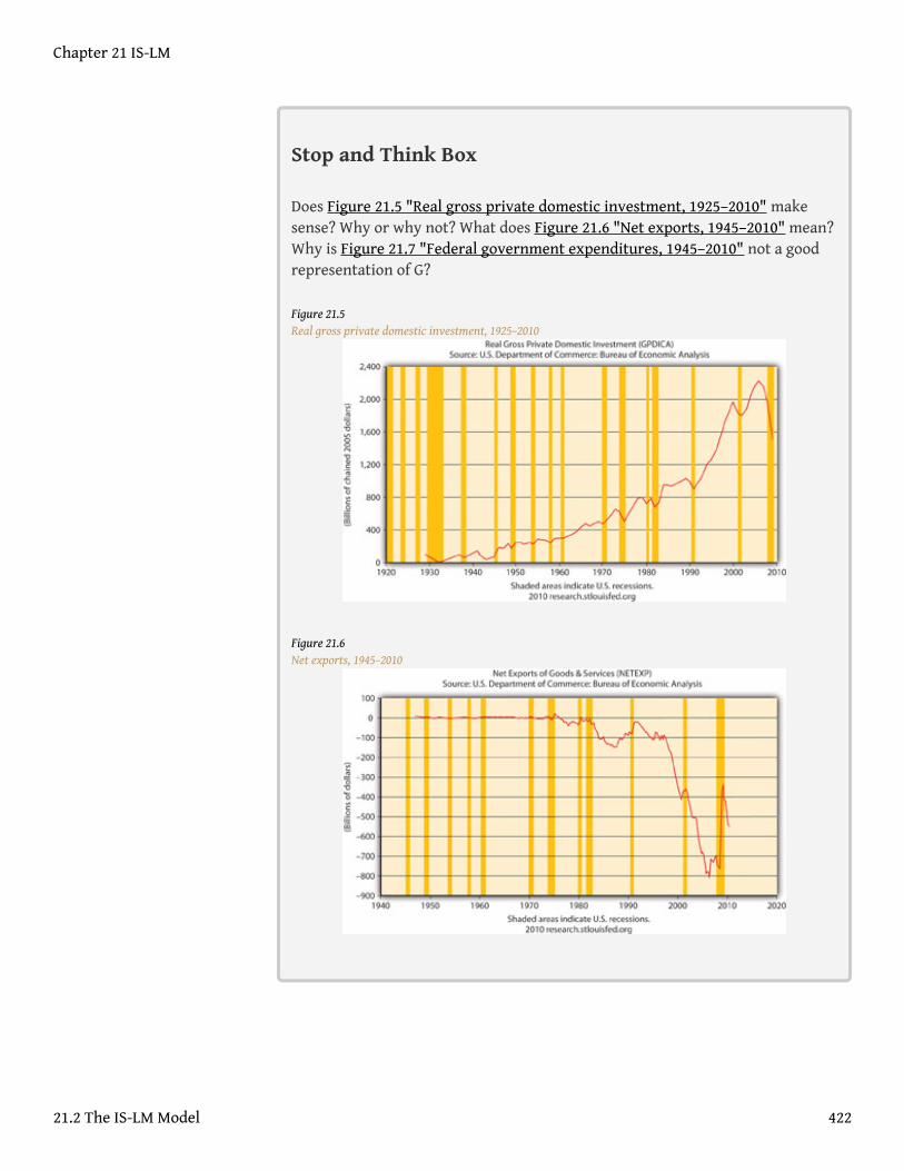
Stop and Think Box
Does Figure 21.5 "Real gross private domestic investment, 1925–2010" makesense? Why or why not? What does Figure 21.6 "Net exports, 1945–2010" mean?Why is Figure 21.7 "Federal government expenditures, 1945–2010" not a goodrepresentation of G?
Figure 21.5Real gross private domestic investment, 1925–2010
Figure 21.6Net exports, 1945–2010
Chapter 21 IS-LM
21.2 The IS-LM Model 422
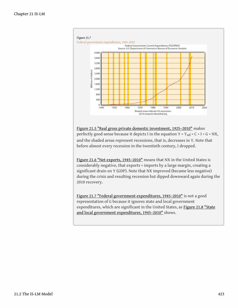
Figure 21.7Federal government expenditures, 1945–2010
Figure 21.5 "Real gross private domestic investment, 1925–2010" makesperfectly good sense because it depicts I in the equation Y = Yad = C + I + G + NX,
and the shaded areas represent recessions, that is, decreases in Y. Note thatbefore almost every recession in the twentieth century, I dropped.
Figure 21.6 "Net exports, 1945–2010" means that NX in the United States isconsiderably negative, that exports < imports by a large margin, creating asignificant drain on Y (GDP). Note that NX improved (became less negative)during the crisis and resulting recession but dipped downward again during the2010 recovery.
Figure 21.7 "Federal government expenditures, 1945–2010" is not a goodrepresentation of G because it ignores state and local governmentexpenditures, which are significant in the United States, as Figure 21.8 "Stateand local government expenditures, 1945–2010" shows.
Chapter 21 IS-LM
21.2 The IS-LM Model 423
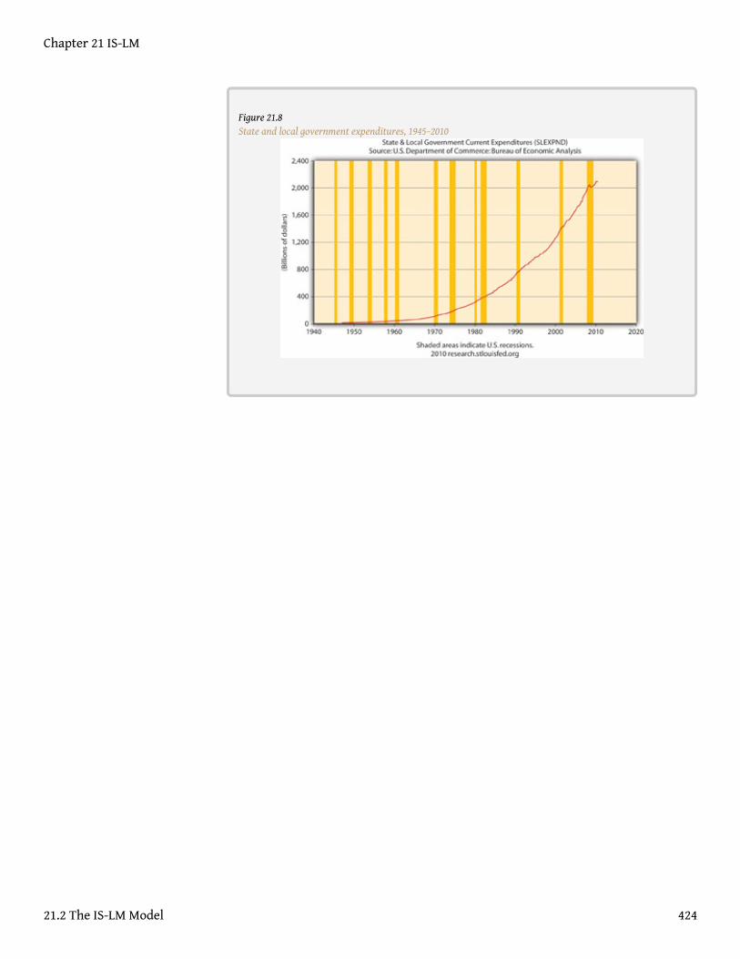
Figure 21.8State and local government expenditures, 1945–2010
Chapter 21 IS-LM
21.2 The IS-LM Model 424
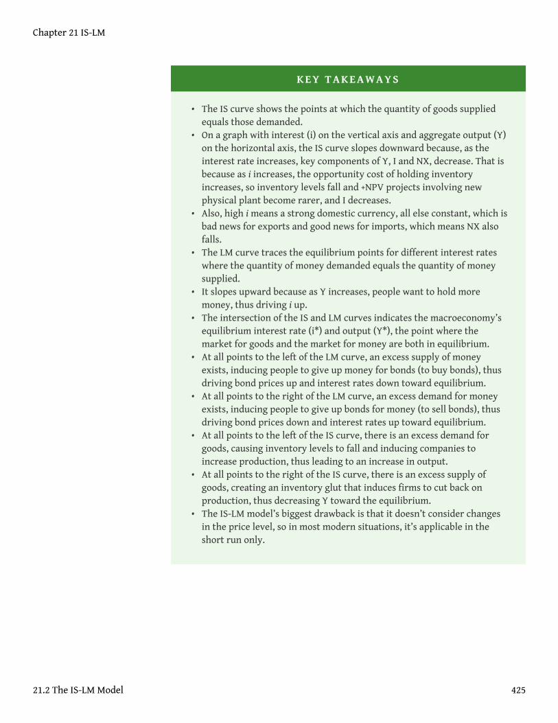
KEY TAKEAWAYS
• The IS curve shows the points at which the quantity of goods suppliedequals those demanded.
• On a graph with interest (i) on the vertical axis and aggregate output (Y)on the horizontal axis, the IS curve slopes downward because, as theinterest rate increases, key components of Y, I and NX, decrease. That isbecause as i increases, the opportunity cost of holding inventoryincreases, so inventory levels fall and +NPV projects involving newphysical plant become rarer, and I decreases.
• Also, high i means a strong domestic currency, all else constant, which isbad news for exports and good news for imports, which means NX alsofalls.
• The LM curve traces the equilibrium points for different interest rateswhere the quantity of money demanded equals the quantity of moneysupplied.
• It slopes upward because as Y increases, people want to hold moremoney, thus driving i up.
• The intersection of the IS and LM curves indicates the macroeconomy’sequilibrium interest rate (i*) and output (Y*), the point where themarket for goods and the market for money are both in equilibrium.
• At all points to the left of the LM curve, an excess supply of moneyexists, inducing people to give up money for bonds (to buy bonds), thusdriving bond prices up and interest rates down toward equilibrium.
• At all points to the right of the LM curve, an excess demand for moneyexists, inducing people to give up bonds for money (to sell bonds), thusdriving bond prices down and interest rates up toward equilibrium.
• At all points to the left of the IS curve, there is an excess demand forgoods, causing inventory levels to fall and inducing companies toincrease production, thus leading to an increase in output.
• At all points to the right of the IS curve, there is an excess supply ofgoods, creating an inventory glut that induces firms to cut back onproduction, thus decreasing Y toward the equilibrium.
• The IS-LM model’s biggest drawback is that it doesn’t consider changesin the price level, so in most modern situations, it’s applicable in theshort run only.
Chapter 21 IS-LM
21.2 The IS-LM Model 425
21.3 Suggested Reading
Dimand, Robert, Edward Nelson, Robert Lucas, Mauro Boianovsky, David Colander,Warren Young, et al. The IS-LM Model: Its Rise, Fall, and Strange Persistence. Raleigh,NC: Duke University Press, 2005.
Young, Warren, and Ben-Zion Zilbefarb. IS-LM and Modern Macroeconomics. NewYork: Springer, 2001.
Chapter 21 IS-LM
426
Chapter 22
IS-LM in Action
CHAPTER OBJECTIVES
By the end of this chapter, students should be able to:
1. Explain what causes the liquidity preference–money (LM) curve to shiftand why.
2. Explain what causes the investment-savings (IS) curve to shift and why.3. Explain the difference between monetary and fiscal stimulus in the
short term and why the difference is important.4. Explain what happens when the IS-LM model is used to tackle the long
term by taking changes in the price level into account.5. Describe the aggregate demand curve and explain what causes it to shift.
427
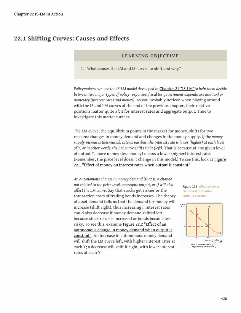
Figure 22.1 Effect of moneyon interest rates whenoutput is constant
22.1 Shifting Curves: Causes and Effects
LEARNING OBJECTIVE
1. What causes the LM and IS curves to shift and why?
Policymakers can use the IS-LM model developed in Chapter 21 "IS-LM"to help them decidebetween two major types of policy responses, fiscal (or government expenditure and tax) ormonetary (interest rates and money). As you probably noticed when playing aroundwith the IS and LM curves at the end of the previous chapter, their relativepositions matter quite a bit for interest rates and aggregate output. Time toinvestigate this matter further.
The LM curve, the equilibrium points in the market for money, shifts for tworeasons: changes in money demand and changes in the money supply. If the moneysupply increases (decreases), ceteris paribus, the interest rate is lower (higher) at each levelof Y, or in other words, the LM curve shifts right (left). That is because at any given levelof output Y, more money (less money) means a lower (higher) interest rate.(Remember, the price level doesn’t change in this model.) To see this, look at Figure22.1 "Effect of money on interest rates when output is constant".
An autonomous change in money demand (that is, a changenot related to the price level, aggregate output, or i) will alsoaffect the LM curve. Say that stocks get riskier or thetransaction costs of trading bonds increases. The theoryof asset demand tells us that the demand for money willincrease (shift right), thus increasing i. Interest ratescould also decrease if money demand shifted leftbecause stock returns increased or bonds became lessrisky. To see this, examine Figure 22.2 "Effect of anautonomous change in money demand when output isconstant". An increase in autonomous money demandwill shift the LM curve left, with higher interest rates ateach Y; a decrease will shift it right, with lower interestrates at each Y.
Chapter 22 IS-LM in Action
428
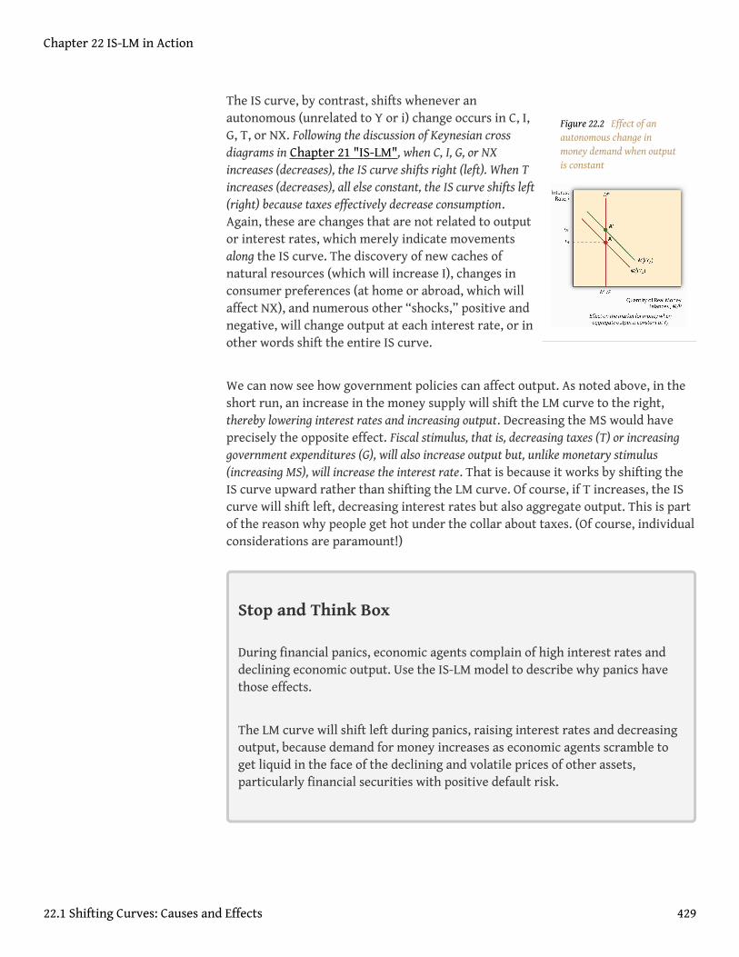
Figure 22.2 Effect of anautonomous change inmoney demand when outputis constant
The IS curve, by contrast, shifts whenever anautonomous (unrelated to Y or i) change occurs in C, I,G, T, or NX. Following the discussion of Keynesian crossdiagrams in Chapter 21 "IS-LM", when C, I, G, or NXincreases (decreases), the IS curve shifts right (left). When Tincreases (decreases), all else constant, the IS curve shifts left(right) because taxes effectively decrease consumption.Again, these are changes that are not related to outputor interest rates, which merely indicate movementsalong the IS curve. The discovery of new caches ofnatural resources (which will increase I), changes inconsumer preferences (at home or abroad, which willaffect NX), and numerous other “shocks,” positive andnegative, will change output at each interest rate, or inother words shift the entire IS curve.
We can now see how government policies can affect output. As noted above, in theshort run, an increase in the money supply will shift the LM curve to the right,thereby lowering interest rates and increasing output. Decreasing the MS would haveprecisely the opposite effect. Fiscal stimulus, that is, decreasing taxes (T) or increasinggovernment expenditures (G), will also increase output but, unlike monetary stimulus(increasing MS), will increase the interest rate. That is because it works by shifting theIS curve upward rather than shifting the LM curve. Of course, if T increases, the IScurve will shift left, decreasing interest rates but also aggregate output. This is partof the reason why people get hot under the collar about taxes. (Of course, individualconsiderations are paramount!)
Stop and Think Box
During financial panics, economic agents complain of high interest rates anddeclining economic output. Use the IS-LM model to describe why panics havethose effects.
The LM curve will shift left during panics, raising interest rates and decreasingoutput, because demand for money increases as economic agents scramble toget liquid in the face of the declining and volatile prices of other assets,particularly financial securities with positive default risk.
Chapter 22 IS-LM in Action
22.1 Shifting Curves: Causes and Effects 429

Figure 22.3 "Predicted effects of changes in major macroeconomicvariables"summarizes.
Figure 22.3 Predicted effects of changes in major macroeconomic variables
Stop and Think Box
Describe Hamilton’s Law (née Bagehot’s Law) in terms of the IS-LM model. Hint:Hamilton and Bagehot argued that, during a financial panic, the lender of lastresort needs to increase the money supply by lending to all comers who presentwhat would be considered adequate collateral in normal times.
During financial panics, the LM curve shifts left as people flee risky assets formoney, thereby inducing the interest rate to climb and output to fall. Hamiltonand Bagehot argued that monetary authorities should respond by nipping theproblem in the bud, so to speak, by increasing MS directly, shifting the LMcurve back to somewhere near its pre-panic position.
Chapter 22 IS-LM in Action
22.1 Shifting Curves: Causes and Effects 430
KEY TAKEAWAYS
• The LM curve shifts right (left) when the money supply (real moneybalances) increases (decreases).
• It also shifts left (right) when money demand increases (decreases).• The easiest way to see this is to first imagine a graph where money
demand is fixed and the money supply increases (shifts right), leading toa lower interest rate, and vice versa.
• Then imagine a fixed MS and a shift upward in money demand, leadingto a higher interest rate, and vice versa.
• The IS curve shifts right (left) when C, I, G, or NX increase (decrease) orT decreases (increases).
• This relates directly to the Keynesian cross diagrams and the equation Y= C + I + G + NX discussed in Chapter 21 "IS-LM", and also to the analysisof taxes as a decrease in consumption expenditure C.
Chapter 22 IS-LM in Action
22.1 Shifting Curves: Causes and Effects 431
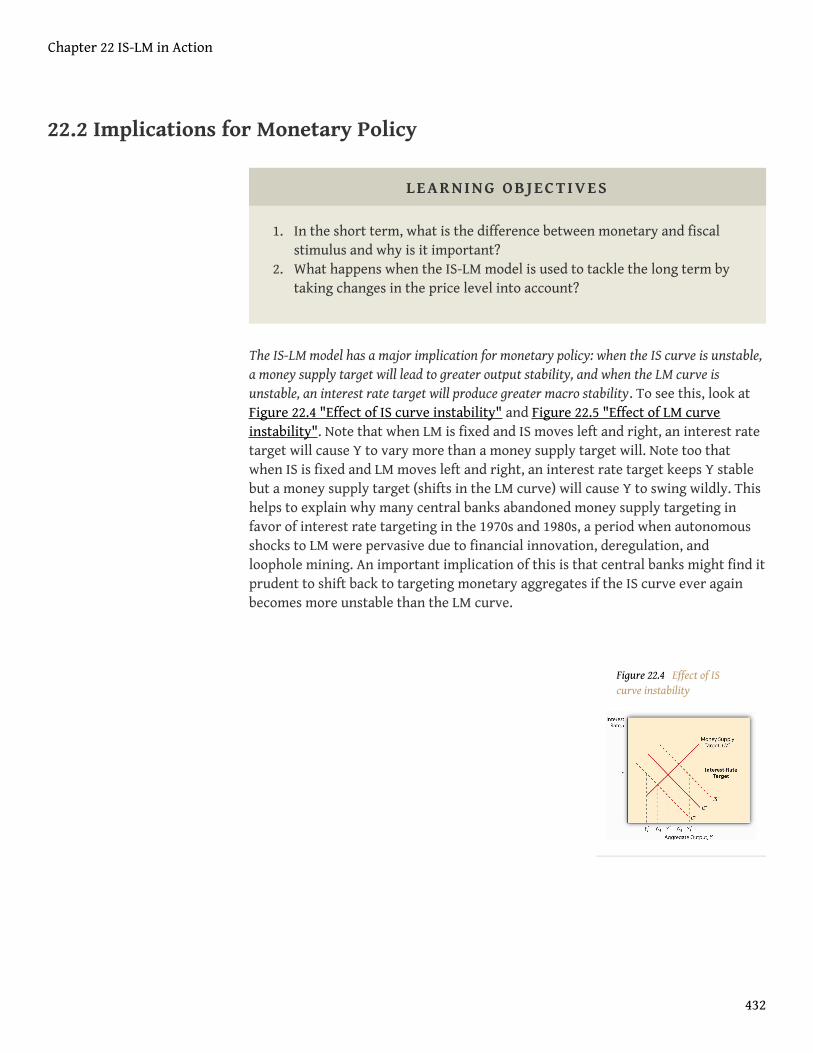
Figure 22.4 Effect of IScurve instability
22.2 Implications for Monetary Policy
LEARNING OBJECTIVES
1. In the short term, what is the difference between monetary and fiscalstimulus and why is it important?
2. What happens when the IS-LM model is used to tackle the long term bytaking changes in the price level into account?
The IS-LM model has a major implication for monetary policy: when the IS curve is unstable,a money supply target will lead to greater output stability, and when the LM curve isunstable, an interest rate target will produce greater macro stability. To see this, look atFigure 22.4 "Effect of IS curve instability" and Figure 22.5 "Effect of LM curveinstability". Note that when LM is fixed and IS moves left and right, an interest ratetarget will cause Y to vary more than a money supply target will. Note too thatwhen IS is fixed and LM moves left and right, an interest rate target keeps Y stablebut a money supply target (shifts in the LM curve) will cause Y to swing wildly. Thishelps to explain why many central banks abandoned money supply targeting infavor of interest rate targeting in the 1970s and 1980s, a period when autonomousshocks to LM were pervasive due to financial innovation, deregulation, andloophole mining. An important implication of this is that central banks might find itprudent to shift back to targeting monetary aggregates if the IS curve ever againbecomes more unstable than the LM curve.
Chapter 22 IS-LM in Action
432

Figure 22.5 Effect of LMcurve instability
As noted in Chapter 21 "IS-LM", the policy power of the IS-LM is severely limited by its short-run assumption that theprice level doesn’t change. Attempts to tweak the IS-LM modelto accommodate price level changes led to the creation of anentirely new model called aggregate demand and supply. Thekey is the addition of a new concept, called the naturalrate level of output1, Ynrl, the rate of output at which
the price level is stable in the long run. When actualoutput (Y*) is below the natural rate, prices will fall;when it is above the natural rate, prices will rise.
The IS curve is stated in real terms because it representsequilibrium in the goods market, the real part of theeconomy. Changes in the price level therefore do not affect C, I, G, T, or NX or the IScurve. The LM curve, however, is affected by changes in the price level, shifting to the leftwhen prices rise and to the right when they fall. This is because, holding the nominal MSconstant, rising prices decrease real money balances, which we know shifts the LMcurve to the left.
So suppose an economy is in equilibrium at Ynrl, when some monetary stimulus in
the form of an increased MS shifts the LM curve to the right. As noted above, in theshort term, interest rates will come down and output will increase. But because Y*is greater than Ynrl, prices will rise, shifting the LM curve back to where it started,
give or take. So output and the interest rate are the same but prices are higher. Economistscall this long-run monetary neutrality.
Fiscal stimulus, as we saw above, shifts the IS curve to the right, increasing outputbut also the interest rate. Because Y* is greater than Ynrl, prices will rise and the LM
curve will shift left, reducing output, increasing the interest rate higher still, andraising the price level! You just can’t win in the long run, in the sense that policymakerscannot make Y* exceed Ynrl. Rendering policymakers impotent did not win the IS-LM
model many friends, so researchers began to develop a new model that relates theprice level to aggregate output.
1. The rate of output at which theprice level has no tendency torise or fall.
Chapter 22 IS-LM in Action
22.2 Implications for Monetary Policy 433
Stop and Think Box
As explained in Chapter 19 "International Monetary Regimes", under the goldstandard (GS), money flows in and out of countries automatically, in responseto changes in the price of international bills of exchange. From the standpointof the IS-LM model, what is the problem with that aspect of the GS?
As noted above, decreases in MS lead to a leftward shift of the LM curve,leading to higher interest rates and lower output. Higher interest rates, in turn,could lead to a financial panic or a decrease in C or I, causing a shift left in theIS curve, further reducing output but relieving some of the pressure on i. (Notethat NX would not be affected under the GS because the exchange rate wasfixed, moving only within very tight bands, so a higher i would not cause thedomestic currency to strengthen.)
KEY TAKEAWAYS
• Monetary stimulus, that is, increasing the money supply, causes the LMcurve to shift right, resulting in higher output and lower interest rates.
• Fiscal stimulus, that is, increasing government spending and/ordecreasing taxes, shifts the IS curve to the right, raising interest rateswhile increasing output.
• The higher interest rates are problematic because they can crowd out C,I, and NX, moving the IS curve left and reducing output.
• The IS-LM model predicts that, in the long run, policymakers areimpotent.
• Policymakers can raise the price level but they can’t get Y* permanentlyabove Ynrl or the natural rate level of output.
• That is because whenever Y* exceeds Ynrl, prices rise, shifting the LMcurve to the left by reducing real money balances (which happens whenthere is a higher price level coupled with an unchanged MS).
• That, in turn, eradicates any gains from monetary or fiscal stimulus.
Chapter 22 IS-LM in Action
22.2 Implications for Monetary Policy 434
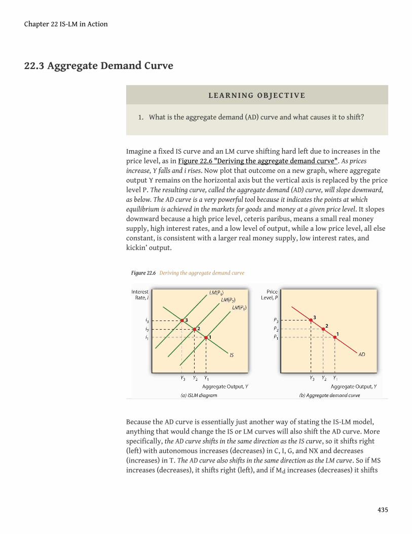
22.3 Aggregate Demand Curve
LEARNING OBJECTIVE
1. What is the aggregate demand (AD) curve and what causes it to shift?
Imagine a fixed IS curve and an LM curve shifting hard left due to increases in theprice level, as in Figure 22.6 "Deriving the aggregate demand curve". As pricesincrease, Y falls and i rises. Now plot that outcome on a new graph, where aggregateoutput Y remains on the horizontal axis but the vertical axis is replaced by the pricelevel P. The resulting curve, called the aggregate demand (AD) curve, will slope downward,as below. The AD curve is a very powerful tool because it indicates the points at whichequilibrium is achieved in the markets for goods and money at a given price level. It slopesdownward because a high price level, ceteris paribus, means a small real moneysupply, high interest rates, and a low level of output, while a low price level, all elseconstant, is consistent with a larger real money supply, low interest rates, andkickin’ output.
Figure 22.6 Deriving the aggregate demand curve
Because the AD curve is essentially just another way of stating the IS-LM model,anything that would change the IS or LM curves will also shift the AD curve. Morespecifically, the AD curve shifts in the same direction as the IS curve, so it shifts right(left) with autonomous increases (decreases) in C, I, G, and NX and decreases(increases) in T. The AD curve also shifts in the same direction as the LM curve. So if MSincreases (decreases), it shifts right (left), and if Md increases (decreases) it shifts
Chapter 22 IS-LM in Action
435

left (right), as in Figure 22.3 "Predicted effects of changes in major macroeconomicvariables".
KEY TAKEAWAYS
• The aggregate demand curve is a downward sloping curve plotted on agraph with Y on the horizontal axis and the price level on the verticalaxis.
• The AD curve represents IS-LM equilibrium points, that is, equilibriumin the market for both goods and money.
• It slopes downward because, as the price level increases, the LM curveshifts left as real money balances fall.
• AD shifts in the same direction as the IS or LM curves, so anything thatshifts those curves shifts AD in precisely the same direction and for thesame reasons.
Chapter 22 IS-LM in Action
22.3 Aggregate Demand Curve 436
22.4 Suggested Reading
Dimand, Robert, Edward Nelson, Robert Lucas, Mauro Boianovsky, David Colander,Warren Young, et al. The IS-LM Model: Its Rise, Fall, and Strange Persistence. Raleigh,NC: Duke University Press, 2005.
Young, Warren, and Ben-Zion Zilbefarb. IS-LM and Modern Macroeconomics. NewYork: Springer, 2001.
Chapter 22 IS-LM in Action
437
Chapter 23
Aggregate Supply and Demand, the Growth Diamond, andFinancial Shocks
CHAPTER OBJECTIVES
By the end of this chapter, students should be able to:
1. Describe the aggregate demand (AD) curve and explain why it slopesdownward.
2. Describe what shifts the AD curve and explain why.3. Describe the short-run aggregate supply (AS) curve and explain why it
slopes upward.4. Describe what shifts the short-run AS curve and explain why.5. Describe the long-run aggregate supply (ASL) curve, and explain why it
is vertical and what shifts it.6. Explain the term long term and its importance for policymakers.7. Describe the growth diamond model of economic growth and its
importance.8. Explain how financial shocks affect the real economy.
438
23.1 Aggregate Demand
LEARNING OBJECTIVES
1. What is the AD curve and why does it slope downward?2. What shifts the AD curve and why?
We learned in Chapter 22 "IS-LM in Action" that the IS-LM model isn’t entirelyagreeable to policymakers because it examines only the short term, and whenpressed into service for the long-term, or changes in the price level, it suggests thatpolicy initiatives are more likely to mess matters up than to improve them. Inresponse, economists developed a new theory, aggregate demand and supply, thatrelates the price level to the total final goods and services demanded (aggregatedemand [AD]) and the total supplied (aggregate supply [AS]). This new framework isattractive for several reasons: (1) it can be used to examine both the short and the long run;(2) it takes a form similar to the microeconomic price theory model of supply and demand, soit is familiar; and (3) it gives policymakers some grounds for implementing activist economicpolicies. To understand aggregate demand and supply theory, we need tounderstand how each of the curves is derived.
The aggregate demand curve can be derived three ways, through the IS-LM model asdescribed at the end of Chapter 22 "IS-LM in Action", with help from the quantity theoryof money, or directly from its components. Remember that Y = C + I + G + NX. As the pricelevel falls, ceteris paribus, real money balances are higher. That spells a lowerinterest rate, as we learned in Chapter 5 "The Economics of Interest-RateFluctuations". A lower interest rate, in turn, means an increase in I (and hence Y). Alower interest rate also means a lower exchange rate and, as explained in Chapter18 "Foreign Exchange", more exports and fewer imports. So NX also increases. (Cmight be positively affected by lower i as well.) As the price level increases, theopposite occurs. So the AD curve slopes downward.
Chapter 23 Aggregate Supply and Demand, the Growth Diamond, and Financial Shocks
439
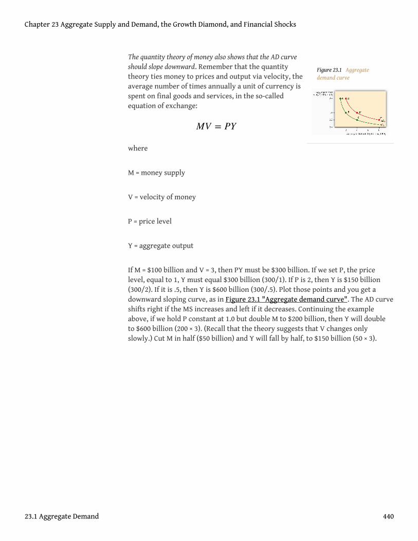
Figure 23.1 Aggregatedemand curve
The quantity theory of money also shows that the AD curveshould slope downward. Remember that the quantitytheory ties money to prices and output via velocity, theaverage number of times annually a unit of currency isspent on final goods and services, in the so-calledequation of exchange:
where
M = money supply
V = velocity of money
P = price level
Y = aggregate output
If M = $100 billion and V = 3, then PY must be $300 billion. If we set P, the pricelevel, equal to 1, Y must equal $300 billion (300/1). If P is 2, then Y is $150 billion(300/2). If it is .5, then Y is $600 billion (300/.5). Plot those points and you get adownward sloping curve, as in Figure 23.1 "Aggregate demand curve". The AD curveshifts right if the MS increases and left if it decreases. Continuing the exampleabove, if we hold P constant at 1.0 but double M to $200 billion, then Y will doubleto $600 billion (200 × 3). (Recall that the theory suggests that V changes onlyslowly.) Cut M in half ($50 billion) and Y will fall by half, to $150 billion (50 × 3).
MV = PY
Chapter 23 Aggregate Supply and Demand, the Growth Diamond, and Financial Shocks
23.1 Aggregate Demand 440
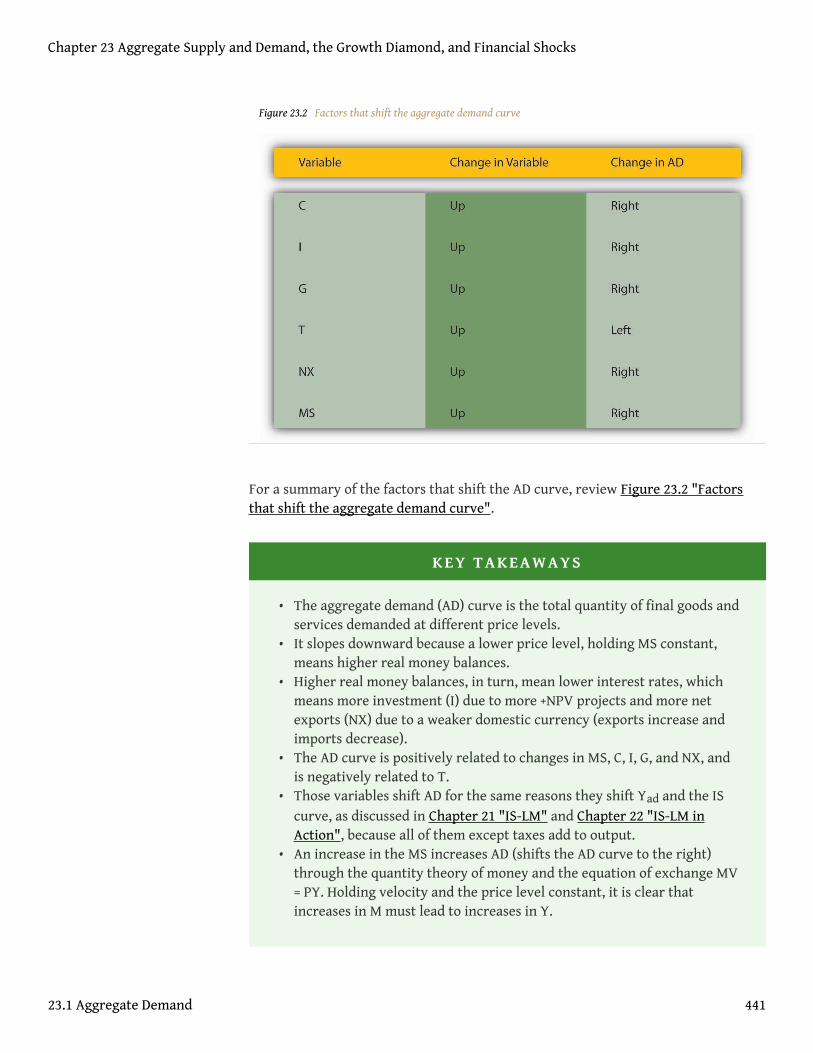
Figure 23.2 Factors that shift the aggregate demand curve
For a summary of the factors that shift the AD curve, review Figure 23.2 "Factorsthat shift the aggregate demand curve".
KEY TAKEAWAYS
• The aggregate demand (AD) curve is the total quantity of final goods andservices demanded at different price levels.
• It slopes downward because a lower price level, holding MS constant,means higher real money balances.
• Higher real money balances, in turn, mean lower interest rates, whichmeans more investment (I) due to more +NPV projects and more netexports (NX) due to a weaker domestic currency (exports increase andimports decrease).
• The AD curve is positively related to changes in MS, C, I, G, and NX, andis negatively related to T.
• Those variables shift AD for the same reasons they shift Yad and the IScurve, as discussed in Chapter 21 "IS-LM" and Chapter 22 "IS-LM inAction", because all of them except taxes add to output.
• An increase in the MS increases AD (shifts the AD curve to the right)through the quantity theory of money and the equation of exchange MV= PY. Holding velocity and the price level constant, it is clear thatincreases in M must lead to increases in Y.
Chapter 23 Aggregate Supply and Demand, the Growth Diamond, and Financial Shocks
23.1 Aggregate Demand 441
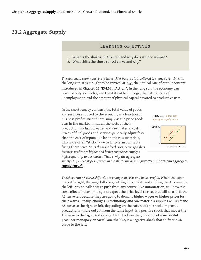
Figure 23.3 Short-runaggregate supply curve
23.2 Aggregate Supply
LEARNING OBJECTIVES
1. What is the short-run AS curve and why does it slope upward?2. What shifts the short-run AS curve and why?
The aggregate supply curve is a tad trickier because it is believed to change over time. Inthe long run, it is thought to be vertical at Ynrl, the natural rate of output concept
introduced in Chapter 22 "IS-LM in Action". In the long run, the economy canproduce only so much given the state of technology, the natural rate ofunemployment, and the amount of physical capital devoted to productive uses.
In the short run, by contrast, the total value of goodsand services supplied to the economy is a function ofbusiness profits, meant here simply as the price goodsbear in the market minus all the costs of theirproduction, including wages and raw material costs.Prices of final goods and services generally adjust fasterthan the cost of inputs like labor and raw materials,which are often “sticky” due to long-term contractsfixing their price. So as the price level rises, ceteris paribus,business profits are higher and hence businesses supply ahigher quantity to the market. That is why the aggregatesupply (AS) curve slopes upward in the short run, as in Figure 23.3 "Short-run aggregatesupply curve".
The short-run AS curve shifts due to changes in costs and hence profits. When the labormarket is tight, the wage bill rises, cutting into profits and shifting the AS curve tothe left. Any so-called wage push from any source, like unionization, will have thesame effect. If economic agents expect the price level to rise, that will also shift theAS curve left because they are going to demand higher wages or higher prices fortheir wares. Finally, changes in technology and raw materials supplies will shift theAS curve to the right or left, depending on the nature of the shock. Improvedproductivity (more output from the same input) is a positive shock that moves theAS curve to the right. A shortage due to bad weather, creation of a successfulproducer monopoly or cartel, and the like, is a negative shock that shifts the AScurve to the left.
Chapter 23 Aggregate Supply and Demand, the Growth Diamond, and Financial Shocks
442
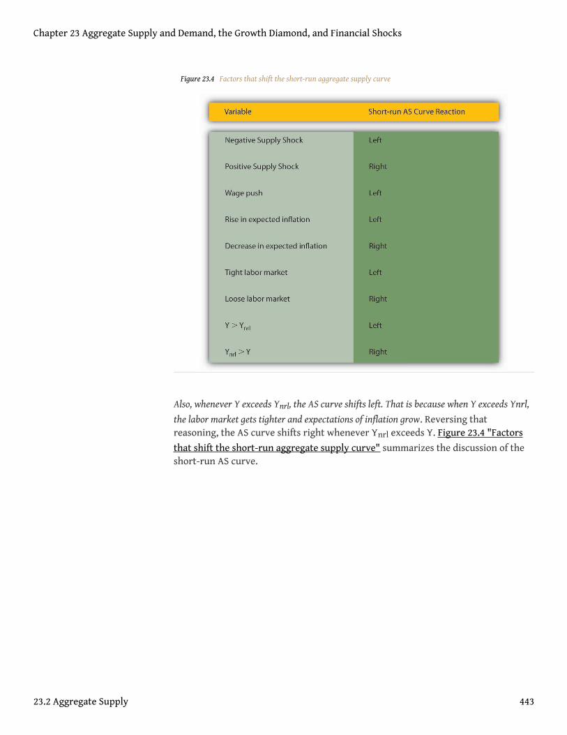
Figure 23.4 Factors that shift the short-run aggregate supply curve
Also, whenever Y exceeds Ynrl, the AS curve shifts left. That is because when Y exceeds Ynrl,
the labor market gets tighter and expectations of inflation grow. Reversing thatreasoning, the AS curve shifts right whenever Ynrl exceeds Y. Figure 23.4 "Factors
that shift the short-run aggregate supply curve" summarizes the discussion of theshort-run AS curve.
Chapter 23 Aggregate Supply and Demand, the Growth Diamond, and Financial Shocks
23.2 Aggregate Supply 443
KEY TAKEAWAYS
• The aggregate supply (AS) curve is the total quantity of final goods andservices supplied at different price levels.
• It slopes upward because wages and other costs are sticky in the shortrun, so higher prices mean more profits (prices minus costs), whichmeans a higher quantity supplied.
• The AS curve shifts left when Y* exceeds Ynrl, and it shifts right when Y*is less than Ynrl.
• In other words, Ynrl is achieved via shifts in the AS curve, particularlythrough labor market “tightness” and inflation expectations.
• When Y* is > Ynrl, the labor market is tight, pushing wages up andstrengthening inflation expectations; when Ynrl is > *Y, the labor marketis loose, keeping wages low and inflation expectations weak.
• Supply shocks, both positive and negative, also shift the AS curve.• Anything (like a so-called wage push or higher raw materials prices) that
decreases business profits shifts AS to the left, while anything thatincreases business profits moves it to the right.
Chapter 23 Aggregate Supply and Demand, the Growth Diamond, and Financial Shocks
23.2 Aggregate Supply 444
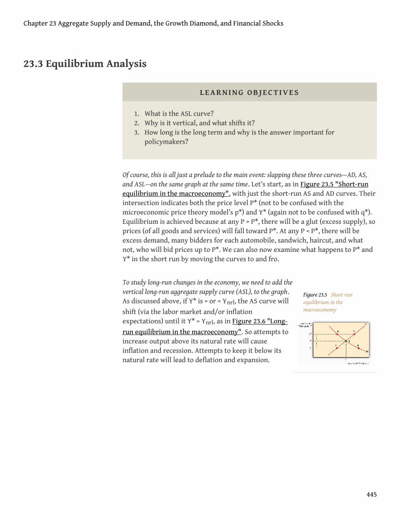
Figure 23.5 Short-runequilibrium in themacroeconomy
23.3 Equilibrium Analysis
LEARNING OBJECTIVES
1. What is the ASL curve?2. Why is it vertical, and what shifts it?3. How long is the long term and why is the answer important for
policymakers?
Of course, this is all just a prelude to the main event: slapping these three curves—AD, AS,and ASL—on the same graph at the same time. Let’s start, as in Figure 23.5 "Short-runequilibrium in the macroeconomy", with just the short-run AS and AD curves. Theirintersection indicates both the price level P* (not to be confused with themicroeconomic price theory model’s p*) and Y* (again not to be confused with q*).Equilibrium is achieved because at any P > P*, there will be a glut (excess supply), soprices (of all goods and services) will fall toward P*. At any P < P*, there will beexcess demand, many bidders for each automobile, sandwich, haircut, and whatnot, who will bid prices up to P*. We can also now examine what happens to P* andY* in the short run by moving the curves to and fro.
To study long-run changes in the economy, we need to add thevertical long-run aggregate supply curve (ASL), to the graph.As discussed above, if Y* is > or < Ynrl, the AS curve will
shift (via the labor market and/or inflationexpectations) until it Y* = Ynrl, as in Figure 23.6 "Long-
run equilibrium in the macroeconomy". So attempts toincrease output above its natural rate will causeinflation and recession. Attempts to keep it below itsnatural rate will lead to deflation and expansion.
Chapter 23 Aggregate Supply and Demand, the Growth Diamond, and Financial Shocks
445
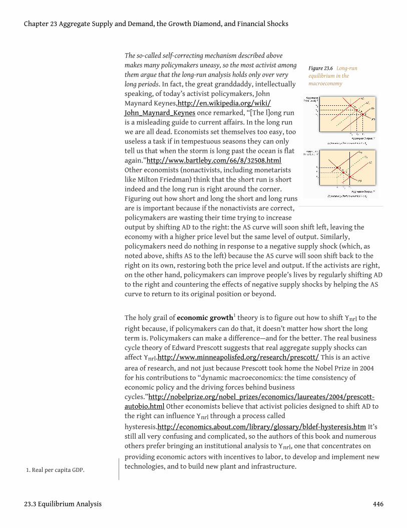
Figure 23.6 Long-runequilibrium in themacroeconomy
The so-called self-correcting mechanism described abovemakes many policymakers uneasy, so the most activist amongthem argue that the long-run analysis holds only over verylong periods. In fact, the great granddaddy, intellectuallyspeaking, of today’s activist policymakers, JohnMaynard Keynes,http://en.wikipedia.org/wiki/John_Maynard_Keynes once remarked, “[The l]ong runis a misleading guide to current affairs. In the long runwe are all dead. Economists set themselves too easy, toouseless a task if in tempestuous seasons they can onlytell us that when the storm is long past the ocean is flatagain.”http://www.bartleby.com/66/8/32508.htmlOther economists (nonactivists, including monetaristslike Milton Friedman) think that the short run is shortindeed and the long run is right around the corner.Figuring out how short and long the short and long runsare is important because if the nonactivists are correct,policymakers are wasting their time trying to increaseoutput by shifting AD to the right: the AS curve will soon shift left, leaving theeconomy with a higher price level but the same level of output. Similarly,policymakers need do nothing in response to a negative supply shock (which, asnoted above, shifts AS to the left) because the AS curve will soon shift back to theright on its own, restoring both the price level and output. If the activists are right,on the other hand, policymakers can improve people’s lives by regularly shifting ADto the right and countering the effects of negative supply shocks by helping the AScurve to return to its original position or beyond.
The holy grail of economic growth1 theory is to figure out how to shift Ynrl to the
right because, if policymakers can do that, it doesn’t matter how short the longterm is. Policymakers can make a difference—and for the better. The real businesscycle theory of Edward Prescott suggests that real aggregate supply shocks canaffect Ynrl.http://www.minneapolisfed.org/research/prescott/ This is an active
area of research, and not just because Prescott took home the Nobel Prize in 2004for his contributions to “dynamic macroeconomics: the time consistency ofeconomic policy and the driving forces behind businesscycles.”http://nobelprize.org/nobel_prizes/economics/laureates/2004/prescott-autobio.html Other economists believe that activist policies designed to shift AD tothe right can influence Ynrl through a process called
hysteresis.http://economics.about.com/library/glossary/bldef-hysteresis.htm It’sstill all very confusing and complicated, so the authors of this book and numerousothers prefer bringing an institutional analysis to Ynrl, one that concentrates on
providing economic actors with incentives to labor, to develop and implement newtechnologies, and to build new plant and infrastructure.1. Real per capita GDP.
Chapter 23 Aggregate Supply and Demand, the Growth Diamond, and Financial Shocks
23.3 Equilibrium Analysis 446

Stop and Think Box
People often believe that wars induce long-term economic growth; however,they are quite wrong. Use Figure 23.7 "Inflation and output during and aftertwo major U.S. wars, the Civil War (1861–1865) and World War I (1917–1918)"and the AS-AD model to explain why people think wars induce growth and whythey are wrong.
Figure 23.7Inflation and output during andafter two major U.S. wars, theCivil War (1861–1865) and WorldWar I (1917–1918)
Y* often increases during wars because AD shifts right because of increases in G(tanks, guns, ships, etc.) and I (new or improved factories to produce tanks,guns, ships, etc.) that exceed decreases in C (wartime rationing) and possiblyNX (trade level decreases and/or subsidies provided to or by allies). Due to theright shift in AD, P* also rises, perhaps giving the illusion of wealth. After thewar, however, two things occur: AD shifts back left as war production ceasesand, to the extent that the long run comes home to roost, AS shifts left. Bothlower Y* and the AD leftward shift decreases the price level. Empirically, warsare indeed often followed by recessions and deflation. Figure 23.7 "Inflation andoutput during and after two major U.S. wars, the Civil War (1861–1865) and
Chapter 23 Aggregate Supply and Demand, the Growth Diamond, and Financial Shocks
23.3 Equilibrium Analysis 447
World War I (1917–1918)" shows what happened to prices and output in theUnited States during and after the Civil War (1861–1865) and World War I(1914–1918; direct U.S. involvement, 1917–1918), respectively. The last bastionof the warmongers is the claim that, by inducing technological development,wars cause Ynrl to shift right. Wars do indeed speed research and development,
but getting a few new gizmos a few years sooner is not worth the wartimedestruction of great masses of human and physical capital.
KEY TAKEAWAYS
• The ASL is the amount of output that is obtainable in the long run giventhe available labor, technology, and physical capital set.
• It is vertical because it is insensitive to changes in the price level.• Economists are not entirely certain why ASL shifts. Some point to
hysteresis, others to real business cycles, still others to institutionalimprovements like the growth diamond.
• Nobody knows how long the long term is, but the answer is importantfor one’s attitude toward economic policymaking.
• Those who favor activist policies think the long term is a long way offindeed, so policymakers can benefit the economy by shifting AD and ASto the right.
• Those who are suspicious of interventionist policies think that the longrun will soon be upon us, so interventionist policies cannot help theeconomy for long because output must soon return to Ynrl.
Chapter 23 Aggregate Supply and Demand, the Growth Diamond, and Financial Shocks
23.3 Equilibrium Analysis 448
23.4 The Growth Diamond
LEARNING OBJECTIVE
1. What is the growth diamond and why is it important?
Over the last two decades or so, many scholars, including one of the authors of thistextbook (Wright), have examined the link between financial development andeconomic growth. They have found that financial repression, severe underdevelopment offinancial intermediaries and markets, can stymie growth and that financial developmentpaves the way for growth. The reason is clear: by reducing asymmetric informationand tapping economies of scale (and scope), the financial system efficiently linksinvestors to entrepreneurs, ensuring that society’s scarce resources are allocated totheir highest valued uses and that innovative ideas get a fair trial.
The research agenda of some of those scholars, including the author of thistextbook, has recently broadened to include more of the institutional factors thatenhance or reduce economic growth, sustained rightward movements of Ynrl. A
leading model, set forth by three economic historians who teach economics at NewYork University’s Stern School of Business,http://w4.stern.nyu.edu/economics/facultystaff.cfm?doc_id=1019 is called the growth diamond or diamond ofsustainable growth.http://w4.stern.nyu.edu/sternbusiness/spring_2007/sustainableGrowth.html Imagine a baseball or softball diamond. At the bottom ofthe diamond is home plate, the most important base in the game, where the playerboth begins and, if successful, ends his or her journey. Looking out from home, firstbase is at the right corner; second base is at the top of the diamond, dead ahead;and third base is at the diamond’s left corner. To score a run, a player must returnto home plate after touching first, second, and third base, in that order. Countries areno different than ballplayers in this regard. For a country to get rich, it needs to progressfrom base to base in the proper order.
In the growth diamond, home plate is represented by government, first base by thefinancial system, second base by entrepreneurs, and third base by management. Tosucceed economically, as depicted in Figure 23.8 "The growth diamond", a countrymust first possess a solid home plate, a government that at a minimum protects thelives, liberty, and property of its citizens. Next, it must develop an efficient financialsystem capable of linking savers/investors to people with good business ideas, theentrepreneurs at second base. The managers at third take over after a product hasemerged and matured.
Chapter 23 Aggregate Supply and Demand, the Growth Diamond, and Financial Shocks
449
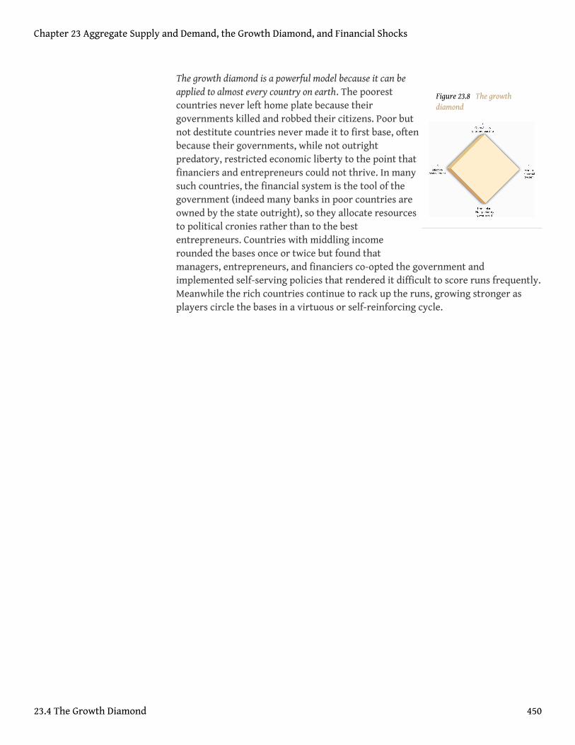
Figure 23.8 The growthdiamond
The growth diamond is a powerful model because it can beapplied to almost every country on earth. The poorestcountries never left home plate because theirgovernments killed and robbed their citizens. Poor butnot destitute countries never made it to first base, oftenbecause their governments, while not outrightpredatory, restricted economic liberty to the point thatfinanciers and entrepreneurs could not thrive. In manysuch countries, the financial system is the tool of thegovernment (indeed many banks in poor countries areowned by the state outright), so they allocate resourcesto political cronies rather than to the bestentrepreneurs. Countries with middling incomerounded the bases once or twice but found thatmanagers, entrepreneurs, and financiers co-opted the government andimplemented self-serving policies that rendered it difficult to score runs frequently.Meanwhile the rich countries continue to rack up the runs, growing stronger asplayers circle the bases in a virtuous or self-reinforcing cycle.
Chapter 23 Aggregate Supply and Demand, the Growth Diamond, and Financial Shocks
23.4 The Growth Diamond 450
Stop and Think Box
In the early nineteenth century, Ontario, Canada (then a colony of GreatBritain), and New York State (then part of a fledgling but independent UnitedStates) enjoyed (perhaps hated is a better word here!) a very similar climate, soiltype, and flora and fauna (plants and animals). Yet the population density inNew York was much higher, farms (ceteris paribus) were worth four times morethere than on the north side of Lake Ontario, and per capita incomes in NewYork dwarfed those of Ontario. What explains those differences?
The growth diamond does. By the early 1800s, the United States, of which NewYork State was a part, had put in place a nonpredatory government and afinancial system that, given the technology of the day, was quite efficient atlinking investors to entrepreneurs, the activities of whom receivedgovernmental sanction and societal support. A nascent management class waseven forming. Ontario, by contrast, was a colony ruled by a distant monarch.Canadians had little incentive to work hard or smart, so they didn’t, and theeconomy languished, largely devoid of banks and other financial intermediariesand securities markets. As late as the 1830s, New York was sometimes “a bettermarket for the sale of Canada exchange on London than Canada itself.”(T. R.Preston, Three Years’ Residence in Canada, from 1837 to 1839, 2 vols., (London:Richard Bentley 1840), 185). Only after they shed their imperial overlords andreformed their domestic governments did Canadians develop an effectivefinancial system and rid themselves of anti-entrepreneurial laws andsentiments. The Canadian economy then grew with rapidity, making Canadaone of the world’s richest countries.
A narrower and more technical explanation of the higher value of New Yorkfarms comparable to Canadian farms in size, soil quality, rainfall, and so forth isthat interest rates were much lower in New York. Valuing a farm is like valuingany income-producing asset. All it takes is to discount the farm’s expectedfuture income stream. Holding expected income constant, the key to theequation becomes the interest rate, which was about four times lower in NewYork (say, 6 percent per year versus 24 percent). Recall that PV = FV/(1 + i). IfFV (next year’s income) in both instances is 100, but i = .24 in Canada and .06 inNew York, an investor would be willing to lease the New York farm for a yearfor 100/1.06 = $94.34, but the Canadian farm for only 100/1.24 = $80.65. Thelonger the time frame, the more the higher Canadian interest rate will bite. Inthe limit, we could price the farms as perpetuities using the equation PV = FV/ifrom Chapter 4 "Interest Rates". That means the New York farm would be
Chapter 23 Aggregate Supply and Demand, the Growth Diamond, and Financial Shocks
23.4 The Growth Diamond 451
worth PV = 100/.06 = $1,666.67, while the Canadian farm would be worth a merePV = 100/.24 = $416.67 (which, of course, times 4 equals the New York farmprice). Canadian land values increased when Canadian interest rates decreasedafter about 1850.
One important implication of the growth diamond is that emerging (from eons of poverty) ortransitioning (from communism) economies that are currently hot, like those of China andIndia, may begin to falter if they do not strengthen their governance, financial,entrepreneurial, and management systems. Some of today’s basket-case economies,including that of Argentina, were once high fliers that ran into an economic brickwall because they inadequately protected property rights, impeded financialdevelopment, and squelched entrepreneurship.
Although currently less analytically rigorous than the AS-AD model, the growthdiamond is more historically grounded than the AS-AD model or any other macromodel and that is important. As storied economist Will Baumol once put it,
We cannot understand current phenomena . . . without systematic examination ofearlier events which affect the present and will continue to exercise profoundeffects tomorrow . . . [T]he long run is important because it is not sensible foreconomists and policymakers to attempt to discern long-run trends and theiroutcomes from the flow of short-run developments, which may be dominated bytransient conditions.Will Baumol, “Productivity Growth, Convergence, and Welfare:What the Long-Run Data Show,” American Economic Review 76 (December 1986):1072–1086, as quoted in Peter L. Bernstein, Against the Gods: The Remarkable Story ofRisk (New York: John Wiley & Sons, 1996), 181.
Chapter 23 Aggregate Supply and Demand, the Growth Diamond, and Financial Shocks
23.4 The Growth Diamond 452
KEY TAKEAWAYS
• The growth diamond is a model of economic growth (increases in realper capita aggregate output) being developed by economic historians atthe Stern School of Business.
• It posits that sustained, long-term economic growth is predicated on theexistence of a nonpredatory government (home plate), an efficientfinancial system (first base), entrepreneurs (second base), and modernmanagement (third base).
• It is important because it explains why some countries are very rich andothers are desperately poor.
• It also explains why some countries, like Argentina, grew rich, only tofall back into poverty.
• Finally, it warns investors that the growth trends of current high flierslike China could reverse if they do not continue to strengthen theirgovernance, financial, entrepreneurial, and management systems.
Chapter 23 Aggregate Supply and Demand, the Growth Diamond, and Financial Shocks
23.4 The Growth Diamond 453
23.5 Financial Shocks
LEARNING OBJECTIVE
1. How do financial shocks and crises affect the real economy?
Another important implication of the growth diamond is that financial crises canhave extremely negative consequences for economic growth. Five shocks2, alone orin combination, have a strong propensity to initiate financial crises:
Increases in uncertainty. When companies cannot plan for the future and wheninvestors feel they cannot estimate future corporate earnings or interest, inflation,or default rates, they tend to play it safe. They hold cash instead of investing in anew factory or equipment. That, of course, reduces aggregate economic activity.
Increases in interest rates. Higher interest rates make business projects less profitableand hence less likely to be completed, a direct blow to gross domestic product(GDP). Also, higher interest rates tend to exacerbate adverse selection bydiscouraging better borrowers but having little or no effect on the borrowingdecisions of riskier companies and individuals. As a result, lenders are saddled withhigher default rates in high interest-rate environments. So, contrary to what onewould think, high rates reduce their desire to lend. To the extent that businessesown government or other bonds, higher interest rates decrease their net worth,leading to balance sheet deterioration, of which we will learn more below. Finally,higher interest rates hurt cash flow (receipts minus expenditures), rendering firmsmore likely to default.
Government fiscal problems. Governments that expend more than they take in viataxes and other revenues have to borrow. The more they borrow, the harder it is forthem to service their loans, raising fears of a default, which decreases the marketprice of their bonds. That hurts the balance sheets of firms that invest ingovernment bonds and may lead to an exchange rate crisis as investors sell assetsdenominated in the local currency in a flight to safety. Precipitous declines in thevalue of local currency causes enormous difficulties for firms that have borrowed inforeign currencies, like dollars, sterling, euro, or yen, because they have to paymore units of local currency than expected for each unit of foreign currency. Manyare unable to do so and they default, increasing uncertainty and asymmetricinformation.
2. In economics, sudden,unexpected changes. Theyusually have adverseconsequences, but some shockscan be salutary. The onesdiscussed here are all bad forthe financial system and hencethe economy.
Chapter 23 Aggregate Supply and Demand, the Growth Diamond, and Financial Shocks
454
Balance sheet deterioration. Whenever a firm’s balance sheet deteriorates, which is tosay, whenever its net worth falls because the value of its assets decreases and/orthe value of its liabilities increases, or because stock market participants value thefirm less highly, the Cerberus of asymmetric information rears its trio of ugly, fang-infested faces. The company now has less at stake, so it might engage in riskieractivities, exacerbating adverse selection. As its net worth declines, moral hazardincreases because it grows more likely to default on existing obligations, in turnbecause it has less at stake. Finally, agency problems become more prevalent asemployee bonuses shrink and stock options become valueless. As employees beginto shirk, steal, and look for other work on company time, productivity plummets,and further declines in profitability cannot be far behind. The same negative cyclecan also be jump-started by an unanticipated deflation, a decrease in the aggregateprice level, because that will make the firm’s liabilities (debts) more onerous in realterms (i.e., adjusted for lower prices).
Banking problems and panics. If anything hurts banks’ balance sheets (like higherthan expected default rates on loans they have made), banks will reduce theirlending to avoid going bankrupt and/or incurring the wrath of regulators. As wehave seen, banks are the most important source of external finance in mostcountries, so their decision to curtail will negatively affect the economy by reducingthe flow of funds between investors and entrepreneurs. If bank balance sheets arehurt badly enough, some may fail. That may trigger the failure of yet more banksfor two reasons. First, banks often owe each other considerable sums. If a big onethat owes much to many smaller banks were to fail, it could endanger the solvencyof the creditor banks. Second, the failure of a few banks may induce the holders ofbanks’ monetary liabilities (today mostly deposits, but in the past, as we’ve seen,also bank notes) to run on the bank, to pull their funds out en masse because theycan’t tell if their bank is a good one or not. The tragic thing about this is that,because all banks engage in fractional reserve banking (which is to say, that nobank keeps enough cash on hand to meet all of its monetary liabilities), runs oftenbecome self-fulfilling prophecies, destroying even solvent institutions in a matter ofdays or even hours. Banking panics and the dead banks they leave in their wakecauses uncertainty, higher interest rates, and balance sheet deterioration, all ofwhich, as we’ve seen, hurt aggregate economic activity.
A downward spiral often ensues. Interest rate increases, stock market declines,uncertainty, balance sheet deterioration, and fiscal imbalances, as detailed above,all tend to increase asymmetric information. That, in turn, causes economic activity todecline, triggering more crises, including bank panics and/or foreign exchange crises, whichincrease asymmetric information yet further. Economic activity again declines, perhapstriggering more crises or an unanticipated decline in the price level. That is thepoint, traditionally, where recessions turn into depressions, unusually long andsteep economic downturns.
Chapter 23 Aggregate Supply and Demand, the Growth Diamond, and Financial Shocks
23.5 Financial Shocks 455
Stop and Think Box
In early 1792, U.S. banks curtailed their lending. That caused a securitiesspeculator and shyster by the name of William Duer to go bankrupt owing largesums of money to hundreds of investors. The uncertainty caused by Duer’ssudden failure caused people to panic, inducing them to sell securities, evengovernment bonds, for cash. By mid-summer, though, the economy was againhumming along nicely. In 1819, banks again curtailed lending, leading to a rashof mercantile failures. People again panicked, this time running on banks (butclutching their government bonds for dear life). Many banks failed andunemployment soared. Economic activity shrank, and it took years to recover.Why did the economy right itself quickly in 1792 but only slowly in 1819?
In 1792, America’s central bank (then the Secretary of the Treasury, AlexanderHamilton, working in conjunction with the Bank of the United States) acted as alender of last resort. By adding liquidity to the economy, the central bankcalmed fears, reduced uncertainty and asymmetric information, and keptinterest rates from spiking and balance sheets from deteriorating further. In1819, the central bank (with a new Treasury secretary and a new bank, theSecond Bank of the United States) crawled under a rock, allowing the initialcrisis to increase asymmetric information, reduce aggregate output, andultimately cause an unexpected debt deflation. Since 1819, America hassuffered from financial crises on numerous occasions. Sometimes they haveended quickly and quietly, as when Alan Greenspan stymied the stock marketcrash of 1987. Other times, like after the stock market crash of 1929, theeconomy did not fare well at all.http://www.amatecon.com/gd/gdcandc.html
Assuming the growth diamond has not been destroyed by the depression,economies will eventually reverse themselves after many companies have gonebankrupt; the balance sheets of surviving firms improve; and uncertainty,asymmetric information, and interest rates decrease (see Chapter 5 "The Economicsof Interest-Rate Fluctuations"). It is better for everyone, however, if financial crises canbe nipped in the bud before they turn ugly. This, as we learned in Chapter 17 "MonetaryPolicy Targets and Goals", is one of the major functions of central banks like theEuropean Central Bank (ECB) and the Fed. Generally, all that the central bank needsto do at the outset of a crisis is to restore confidence, reduce uncertainty, and keepinterest rates in line by adding liquidity (cash) to the economy by acting as a lenderof last resort, helping out banks and other financial intermediaries with loans andbuying government bonds in the open market. As we learned in Chapter 12 "TheFinancial Crisis of 2007–2009", however, sometimes a bailout becomes necessary.
Chapter 23 Aggregate Supply and Demand, the Growth Diamond, and Financial Shocks
23.5 Financial Shocks 456

Figure 23.9 "Anatomy of a financial crisis and economic decline" summarizes thisdiscussion of the ill consequences of financial shocks.
Figure 23.9 Anatomy of a financial crisis and economic decline
Note: At any point the downward spiral can be stopped by adequate central bank intervention.
Source: Text.
But in case you didn’t get the memo, nothing is ever really free. (Well, except forfree goods.)http://en.wikipedia.org/wiki/Free_good When central banks stopfinancial panics, especially when they do so by bailing out failed companies, theyrisk creating moral hazard by teaching market participants that they will shieldthem from risks. That is why some economists, like Allan Meltzer, said “Let ’EmFail,” in the op-ed pages of the Wall Street JournalJuly 21, 2007.http://online.wsj.com/article/SB118498744630073854.html when some hedge fundsran into trouble due to the unexpected deterioration of the subprime mortgagemarket in 2007. Hamilton’s Law (née Bagehot’s Law which, as described in Chapter16 "Monetary Policy Tools", urges lenders of last resort to lend at a penalty rate ongood security) is so powerful precisely because it minimizes moral hazard by
Chapter 23 Aggregate Supply and Demand, the Growth Diamond, and Financial Shocks
23.5 Financial Shocks 457
providing relief only to the more prudent and solvent firms while allowing theriskiest ones to go under.
KEY TAKEAWAYS
• Financial shocks and crises affect the real economy by increasingasymmetric information.
• That, in turn, reduces the amount of funds channeled from investors toentrepreneurs.
• Starved of external finance, businesses cut back production, decreasingaggregate economic activity.
• The conduits include rapidly rising interest rates, foreign exchangecrises, and bank panics.
Chapter 23 Aggregate Supply and Demand, the Growth Diamond, and Financial Shocks
23.5 Financial Shocks 458
23.6 Suggested Reading
Baumol, William, Robert Litan, and Carl Schramm. Good Capitalism, Bad Capitalism,and the Economics of Growth and Prosperity. New Haven, CT: Yale University Press,2007.
Haber, Stephen, Douglass North, and Barry Weingast. Political Institutions andFinancial Development. Stanford, CA: Stanford University Press, 2008.
Powell, Benjamin. Making Poor Nations Rich: Entrepreneurship and the Process ofEconomic Development. Stanford, CA: Stanford University Press, 2008.
Wright, Robert E. One Nation Under Debt: Hamilton, Jefferson, and the History of What WeOwe. New York: McGraw-Hill, 2008.
Chapter 23 Aggregate Supply and Demand, the Growth Diamond, and Financial Shocks
459
Chapter 24
Monetary Policy Transmission Mechanisms
CHAPTER OBJECTIVES
By the end of this chapter, students should be able to:
1. Explain why structural models are generally superior to reduced-formmodels.
2. Describe the types of evidence that can strengthen researchers’conviction that a reduced-form model has the direction of causationright, say, from money (M) to output (Y).
3. Describe the evidence that money matters.4. List and explain several important monetary policy transmission
mechanisms.
460
24.1 Modeling Reality
LEARNING OBJECTIVE
1. Why are structural models generally superior to reduced-form models?
We’ve learned in the last few chapters that monetary policy is not the end-all andbe-all of the economy or even of policymakers’ attempts to manipulate it. But weknew that before. The question before us is, Given what we know of IS-LM and AS-AD,just how important is monetary policy? And how do we know? We’ve got theoriesgalore—notions about how changes in sundry variables, like interest rates, create certainoutcomes, like changes in prices and aggregate output. But how well do those theoriesdescribe reality? To answer those questions, we need empirical evidence, good hardnumbers. We also need to know how scientists and social scientists evaluate suchevidence.
Structural models explicitly link variables from initial cause all the way to final effect viaevery intermediate step along the causal chain. Reduced-form evidence makes assertionsonly about initial causes and ultimate effects, treating the links in between as animpenetrable black box. The quantity theory makes just such a reduced-form claimwhen it asserts that, as the money supply increases, so too does output. In otherwords, the quantity theory is not explicit about the transmission mechanisms1 ofmonetary policy. On the other hand, the assertion that increasing the money supplydecreases interest rates, which spurs investment, which leads to higher output,ceteris paribus, is a structural model. Such a model can be assessed at every link inthe chain: MS up, i down, I up, Y up. If the relationship between MS and Y begins tobreak down, economists with a structural model can try to figure out specificallywhy. Those touting only a reduced-form model will be flummoxed. Structuralmodels also strengthen our confidence that changes in MS cause changes in Y.
Because they leave so much out, reduced-form models may point only to variablesthat are correlated, that rise and fall in tandem over time. Correlation, alas, is notcausation; the link between variables that are only correlated can be easily broken. All sortsof superstitions are based on mere correlation, as their practitioners eventuallydiscover to their chagrin and loss,http://www.dallasobserver.com/2005-09-08/dining/tryst-of-fate/ like those who wear goofy-looking rally caps to win baseballgames.http://en.wikipedia.org/wiki/Rally_cap Reverse causation is also rampant.People who see a high correlation between X and Y often think that X causes Ywhen in fact Y causes X. For example, there is a high correlation between fan
1. How A leads to B in a causalchain; how A is transmitted, soto speak, to B.
Chapter 24 Monetary Policy Transmission Mechanisms
461
attendance levels and home team victories. Somesuperfanshttp://en.wikipedia.org/wiki/Bill_Swerski's_Superfans take this to“prove” that high attendance causes the home team to win by acting as a sixth,tenth, or twelfth player, depending on the sport. Fans have swayed the outcome of afew games, usually by touching baseballs still in play,http://www.usatoday.com/sports/columnist/lopresti/2003-10-15-lopresti_x.htm but the causation mostly runsin the other direction—teams that win many games tend to attract more fans.
Omitted variables can also cloud the connections made by reduced-form models. “Caffeinedrinkers have higher rates of coronary heart disease (CHD) than people who don’tconsume caffeine” is a reduced-form model that probably suffers from omittedvariables in the form of selection biases. In other words, caffeine drinkers drinkcaffeine because they don’t get enough sleep; have hectic, stressful lives; and soforth. It may be that those other factors give them heart attacks, not the caffeineper se. Or the caffeine interacts with those other variables in complex ways that aredifficult to unravel without growing human beings in test tubes (even morealarming!).
Chapter 24 Monetary Policy Transmission Mechanisms
24.1 Modeling Reality 462
Stop and Think Box
A recent reduced-form study shows a high degree of correlation betweensmoking marijuana and bad life outcomes: long stints of unemployment,criminal arrests, higher chance of disability, lower lifetime income, and earlydeath. Does that study effectively condemn pot smoking?
Not nearly as much as it would if it presented a structural model that carefullylaid out and tested the precise chain by which marijuana smoking causes thosebad outcomes. Omitted variables and even reverse causation can be at play inthe reduced-form version. For example, some people smoke pot because theyhave cancer. Some cancer treatments require nasty doses of chemotherapy, theeffect of which is to cause pain and reduce appetite. Taking a toke reduces thepain and restores appetite. Needless to say, such people have lower lifeexpectancies than people without cancer. Therefore, they have lower lifetimeincome and a higher chance of disability and unemployment. Because not allstates have medical marijuana exceptions, they are also more liable to criminalarrest. Similarly, unemployed people might be more likely to take a little MaryJane after lunch or perhaps down a couple of cannabis brownies for dessert,again reversing the direction of causation. A possible omitted variable isselection bias: people who smoke pot might be less educated than those whoabstain from the weed, and it is the dearth of education that leads to highunemployment, more arrests, and so forth. Unfortunately, bad science like thisstudy pervades public discourse. Of course, this does not mean that you shouldgo get yourself a blunt. Study instead. Correlation studies show that studying . .. .
Chapter 24 Monetary Policy Transmission Mechanisms
24.1 Modeling Reality 463
KEY TAKEAWAYS
• Structural models trace the entire causal chain, step by step, allowingresearchers to be pretty confident about the direction of causation andto trace any breakdowns in the model to specific relationships.
• Reduced-form models link initial variables to supposed outcomes via animpenetrable black box.
• The problem is that correlation does not always indicate causation. Xmay increase and decrease with Y, although X does not cause Y becauseY may cause X (reverse causation), or Z (an omitted variable) may causeX and Y.
• Reduced-form models can and have led to all sorts of goofy conclusions,like doctors kill people (they seem to be ubiquitous during plagues,accidents, and the like) and police officers cause crime (the number onthe streets goes up during crime waves, and they are always at crimescenes—very suspicious). In case you can’t tell, I’m being sarcastic.
• On the other hand, reduced-form models are inexpensive compared tostructural ones.
Chapter 24 Monetary Policy Transmission Mechanisms
24.1 Modeling Reality 464
24.2 How Important Is Monetary Policy?
LEARNING OBJECTIVES
1. What types of evidence can strengthen researchers’ conviction that areduced-form model has the direction of causation right, say, from M toY? How?
2. What evidence is there that money matters?
Early Keynesians believed that monetary policy did not matter at all because they could notfind any evidence that interest rates affected planned business investment. Milton Friedmanand Anna Schwartz, another monetarist, countered with a huge tome called A MonetaryHistory of the United States, 1867–1960 which purported to show that the Keynesianshad it all wrong, especially their kooky claim that monetary policy during the GreatDepression had been easy (low real interest rates and MS growth). Nominal rates onrisky securities had in fact soared in 1930–1933, the depths of the depression.Because the price level was falling, real interest rates, via the Fisher Equation, weremuch higher than nominal rates. If you borrowed $100, you’d have to repay only$102 in a year, but those 102 smackers could buy a heck of a lot more goods andservices a year hence. So real rates were more on the order of 8 to 10 percent, whichis pretty darn high. The link between interest rates and investment, themonetarists showed, was between investment and real interest rates, not nominalinterest rates.
As noted above, the early monetarists relied on MV = PY, a reduced-form model. Tostrengthen their conviction that causation indeed ran from M to Y instead of Y to M or someunknown variables A…Z to M and Y, the monetarists relied on three types of empiricalevidence: timing, statistical, and historical. Timing evidence tries to show that increasesin M happen before increases in Y, and not vice versa, relying on the commonplaceassumption that causes occur before their effects. Friedman and Schwartz showedthat money growth slowed before recessions, but the timing was highly variable.Sometimes slowing money growth occurred sixteen months before output turnedsouth; other times, only a few months passed. That is great stuff, but it is hardlyfoolproof because, as Steve Miller points out, time keeps on slipping, slipping,slipping, into the future.http://www.lyricsfreak.com/s/steve+miller/fly+like+an+eagle_20130994.html Maybe a decline in output caused the decline inthe money supply. Changes in M and Y, in other words, could be causing each otherin a sort of virtuous or pernicious cycle or chicken-egg problem. Or again maybethere is a mysterious variable Z running the whole show behind the scenes.
Chapter 24 Monetary Policy Transmission Mechanisms
465
Statistical evidence is subject to the same criticisms plus the old adage that thereare three types of untruths (besides Stephen Colbert’struthiness,http://en.wikipedia.org/wiki/Truthiness of course): lies, damn lies, andstatistics. By changing starting and ending dates, conflating the difference betweenstatistical significance and economicsignificance,http://www.deirdremccloskey.com/articles/stats/preface_ziliak.phpmanipulating the dates of structural breaks, and introducing who knows how manyother subtle little fibs, researchers can make mountains out of molehills, and viceversa. It’s kinda funny that when monetarists used statistical tests, the quantity theory wonand money mattered, but when the early Keynesians conducted the tests, the quantitytheory looked, if not insane, at least inane.
But Friedman and Schwartz had an empirical ace up their sleeves: historicalevidence from periods in which declines in the money supply appear to beexogenous, by which economists mean “caused by something outside the model,”thus eliminating doubts about omitted variables and reverse causation. White-lab-coat scientists (you know, physicists, chemists, and so forth—“real” scientists) knowthat variables change exogenously because they are the ones making the changes.They can do this systematically in dozens, hundreds, even thousands of test tubes,Petri dishes, atomic acceleration experiments, and what not, carefully controllingfor each variable (making sure that everything is ceteris paribus), then measuringand comparing the results. As social scientists, economists cannot run suchexperiments. They can and do turn to history, however, for so-called natural experiments.That’s what the monetarists did, and what they found was that exogenous declinesin MS led to recessions (lower Y*) every time. Economic and financial history wins!(Disclaimer: One of the authors of this textbook [Wright] is a financial historian.) Whilethey did not abandon the view that C, G, I, NX, and T also affect output, Keynesiansnow accept money’s role in helping to determine Y. (A new group, the real-business-cycle theorists associated with the Minneapolis Fed, has recentlychallenged the notion that money matters, but those folks haven’t made it into theland of undergraduate textbooks quite yet.)
Chapter 24 Monetary Policy Transmission Mechanisms
24.2 How Important Is Monetary Policy? 466
KEY TAKEAWAYS
• Timing, statistical, and historical evidence strengthen researchers’belief in causation.
• Timing evidence attempts to show that changes in M occur beforechanges in Y.
• Statistical evidence attempts to show that one model’s predictions arecloser to reality than another’s.
• The problem with stats, though, is that those running the tests appear torig them (consciously or not), so the stats often tell us more about theresearcher than they do about reality.
• Historical evidence, particularly so-called natural experiments in whichvariables change exogenously and hence are analogous to controlledscientific experiments, provide the best sort of evidence on the directionof causation.
• The monetarists showed that there is a strong correlation betweenchanges in the MS and changes in Y and also proffered timing,statistical, and historical evidence of a causal link.
• Historical evidence is the most convincing because it shows that the MSsometimes changed exogenously, that is, for reasons clearly unrelated toY or other plausible causal variables, and that when it did, Y changedwith the expected sign (+ if MS increased, − if it decreased).
Chapter 24 Monetary Policy Transmission Mechanisms
24.2 How Important Is Monetary Policy? 467

24.3 Transmission Mechanisms
LEARNING OBJECTIVE
1. What are monetary policy transmission mechanisms and why are theyimportant?
Most economists accept the proposition that money matters and have beensearching for structural models that delineate the specific transmissionmechanisms between MS and Y. The most basic model says the following:
Expansionary monetary policy (EMP), real interest rates down, investment up, aggregateoutput up
The importance of interest rates for consumer expenditures (especially on durableslike autos, refrigerators, and homes) and net exports has also been recognized,leading to the following:
EMP, ir ↓, I + C + NX ↑, Y ↑
Tobin’s q, the market value of companies divided by the replacement cost of physical capital,is clearly analogous to i and related to I. When q is high, firms sell their highly valuedstock to raise cash and buy new physical plant and build inventories. When q is low,by contrast, firms don’t get much for their stock compared to the cost of physicalcapital, so they don’t sell stock to fund increases in I. By increasing stock prices, theMS may be positively related to q. Thus, another monetary policy transmissionmechanism may be the following:
EMP, Ps↑, q ↑, I ↑, Y↑
The wealth effect is a transmission mechanism whereby expansionary monetary policy leadsto increases in the prices of stocks, homes, collectibles, and other assets, in other words, anincrease in individual wealth. That increase, in turn, induces people to consume more:
EMP, Pa ↑, wealth ↑, C ↑, Y↑
Chapter 24 Monetary Policy Transmission Mechanisms
468
The credit view posits several straightforward transmission mechanisms, including bankloans, asymmetric information, and balance sheets:
EMP, bank deposits ↑, bank loans ↑, I ↑, Y↑
EMP, net worth ↓, asymmetric information ↓, lending ↑, I + C ↑, Y↑
EMP, i ↓, cash flow ↑, asymmetric information ↓, lending ↑, I + C ↑, Y↑
EMP, unanticipated P* ↑, real net worth ↑, asymmetric information ↓, lending ↑, I ↑,Y↑
Asymmetric information (that horrible three-headed hound from Hades) is apowerful and important theory, so scholars’ confidence in these transmissionmechanisms is high.
Chapter 24 Monetary Policy Transmission Mechanisms
24.3 Transmission Mechanisms 469
Stop and Think Box
The Fed thought that it would quickly squelch the recession that began inMarch 2001, yet the downturn lasted until November of that year. The terroristattacks that September worsened matters, but the Fed had hoped to reverse thedrop in Y* well before then. Why was the Fed’s forecast overly optimistic? (Hint:Corporate accounting scandals at Enron, Arthur Andersen, and other firmswere part of the mix.)
The Fed might not have counted on some major monetary policy transmissionmechanisms, including reductions in asymmetric information, being muted bythe accounting scandals. In other words,
EMP, net worth ↑, asymmetric information ↓, lending ↑, I + C ↑, Y↑
EMP, i ↓, cash flow ↑, asymmetric information ↓, lending ↑, I + C ↑, Y↑
EMP, unanticipated P ↑, real net worth ↑, asymmetric information ↓, lending ↑, I↑, Y↑
became something more akin to the following:
EMP, net worth ↑, asymmetric information — (flat or no change), lending —, I +C —, Y —
EMP, i ↑, cash flow ↑, asymmetric information —, lending —, I + C —, Y —
EMP, unanticipated P ↑, real net worth ↑, asymmetric information—, lending —,I —, Y — because asymmetric information remained high due to the fact thateconomic agents felt as though they could no longer count on the truthfulnessof corporate financial statements.
The takeaway of all this for monetary policymakers, and those interested in theirpolicies (including you, as you know from Chapter 1 "Money, Banking, and YourWorld"), is that monetary policy needs to take more into account than just short-term interest rates. Policymakers need to worry about real interest rates, including
Chapter 24 Monetary Policy Transmission Mechanisms
24.3 Transmission Mechanisms 470
long-term rates; unexpected changes in the price level; the interest rates on riskybonds; the prices of other assets, including corporate equities, homes, and the like;the quantity of bank loans; and the bite of adverse selection, moral hazard, and theprincipal-agent problem.
Stop and Think Box
Japan’s economy was going gangbusters until about 1990 or so, when it entereda fifteen-year economic funk. To try to get the Japanese economy moving again,the Bank of Japan lowered short-term interest rates all the way to zero formany years on end, to no avail. Why didn’t the Japanese economy revive due tothe monetary stimulus? What should the Japanese have done instead?
As it turns out, ir stayed quite high because the Japanese expected, and
received, price deflation. Through the Fisher Equation, we know that ir = i − πe,
or real interest rates equal nominal interest rates minus inflation expectations.If πe is negative, which it is when prices are expected to fall, ir will be > i. So ican be 0 but ir can be 1, 2, 3 . . . 10 percent per year if prices are expected todecline by that much. So instead of EMP, ir −, I + C + NX −, Y− the Japanese
experienced ir −, I + C + NX −, Y−. Not good. They should have pumped up the MS
much faster, driving πe from negative whatever to zero or even positive, andthus making real interest rates low or negative, and hence a stimulant. TheJapanese made other mistakes as well, allowing land and equities prices toplummet, thereby nixing the Tobin’s q and wealth effect transmissionmechanisms. They also kept some big shaky banks from failing, which keptlevels of asymmetric information high and bank loan levels low, squelching thecredit channels.
Chapter 24 Monetary Policy Transmission Mechanisms
24.3 Transmission Mechanisms 471
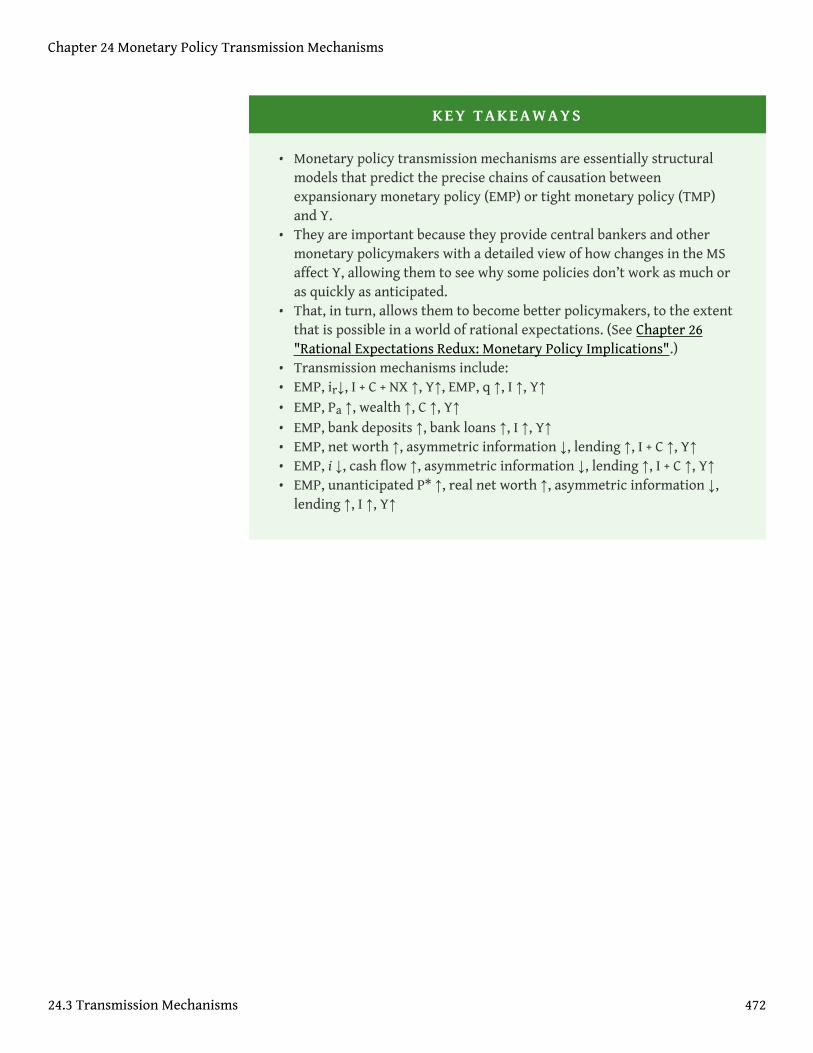
KEY TAKEAWAYS
• Monetary policy transmission mechanisms are essentially structuralmodels that predict the precise chains of causation betweenexpansionary monetary policy (EMP) or tight monetary policy (TMP)and Y.
• They are important because they provide central bankers and othermonetary policymakers with a detailed view of how changes in the MSaffect Y, allowing them to see why some policies don’t work as much oras quickly as anticipated.
• That, in turn, allows them to become better policymakers, to the extentthat is possible in a world of rational expectations. (See Chapter 26"Rational Expectations Redux: Monetary Policy Implications".)
• Transmission mechanisms include:• EMP, ir↓, I + C + NX ↑, Y↑, EMP, q ↑, I ↑, Y↑• EMP, Pa ↑, wealth ↑, C ↑, Y↑• EMP, bank deposits ↑, bank loans ↑, I ↑, Y↑• EMP, net worth ↑, asymmetric information ↓, lending ↑, I + C ↑, Y↑• EMP, i ↓, cash flow ↑, asymmetric information ↓, lending ↑, I + C ↑, Y↑• EMP, unanticipated P* ↑, real net worth ↑, asymmetric information ↓,
lending ↑, I ↑, Y↑
Chapter 24 Monetary Policy Transmission Mechanisms
24.3 Transmission Mechanisms 472
24.4 Suggested Reading
Angeloni, Ignazio, Anil Kashyap, and Benoit Mojon. Monetary Policy Transmission inthe Euro Area. New York: Cambridge University Press, 2004.
Friedman, Milton, and Anna Schwartz. A Monetary History of the United States,1867–1960. Princeton, NJ: Princeton University Press, 1971.
Mahadeva, Lavan, and Peter Sinclair. Monetary Transmission in Diverse Economies. NewYork: Cambridge University Press, 2002.
Chapter 24 Monetary Policy Transmission Mechanisms
473
Chapter 25
Inflation and Money
CHAPTER OBJECTIVES
By the end of this chapter, students should be able to:
1. Describe the strongest evidence for the reduced-form model that linksmoney supply growth to inflation.
2. Explain what the aggregate supply-aggregate demand (AS-AD) model, astructural model, says about money supply growth and the price level.
3. Explain why central bankers allow inflation to occur year after year.4. Define lags and explain their importance.
474
25.1 Empirical Evidence of a Money-Inflation Link
LEARNING OBJECTIVES
1. What is the strongest evidence for the reduced-form model that linksmoney supply growth to inflation?
2. What does the AS-AD model, a structural model, say about money supplygrowth and the price level?
Milton Friedman claimed that “inflation is always and everywhere a monetaryphenomenon.”A Monetary History of the United States, 1867–1960. We know thisisn’t entirely true because, as we saw in Chapter 23 "Aggregate Supply and Demand,the Growth Diamond, and Financial Shocks", negative aggregate supply shocks andincreases in aggregate demand due to fiscal stimulus can also cause the price levelto increase. Large, sustained increases in the price level, however, are indeedcaused by increases in the money supply and only by increases in the money supply.The evidence for this is overwhelming: all periods of hyperinflation from the American andFrench Revolutions to the German hyperinflation following World War I, to more recentepisodes in Latin America and Zimbabwe, have been accompanied by high rates of moneysupply (MS) growth. Moreover, the MS increases in some circumstances wereexogenous, so those episodes were natural experiments that give us confidence thatthe reduced-form model correctly considers money supply as the causal agent andthat reverse causation or omitted variables are unlikely.
Chapter 25 Inflation and Money
475
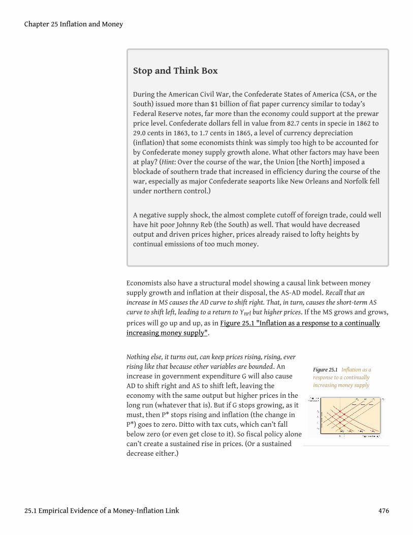
Figure 25.1 Inflation as aresponse to a continuallyincreasing money supply
Stop and Think Box
During the American Civil War, the Confederate States of America (CSA, or theSouth) issued more than $1 billion of fiat paper currency similar to today’sFederal Reserve notes, far more than the economy could support at the prewarprice level. Confederate dollars fell in value from 82.7 cents in specie in 1862 to29.0 cents in 1863, to 1.7 cents in 1865, a level of currency depreciation(inflation) that some economists think was simply too high to be accounted forby Confederate money supply growth alone. What other factors may have beenat play? (Hint: Over the course of the war, the Union [the North] imposed ablockade of southern trade that increased in efficiency during the course of thewar, especially as major Confederate seaports like New Orleans and Norfolk fellunder northern control.)
A negative supply shock, the almost complete cutoff of foreign trade, could wellhave hit poor Johnny Reb (the South) as well. That would have decreasedoutput and driven prices higher, prices already raised to lofty heights bycontinual emissions of too much money.
Economists also have a structural model showing a causal link between moneysupply growth and inflation at their disposal, the AS-AD model. Recall that anincrease in MS causes the AD curve to shift right. That, in turn, causes the short-term AScurve to shift left, leading to a return to Ynrl but higher prices. If the MS grows and grows,
prices will go up and up, as in Figure 25.1 "Inflation as a response to a continuallyincreasing money supply".
Nothing else, it turns out, can keep prices rising, rising, everrising like that because other variables are bounded. Anincrease in government expenditure G will also causeAD to shift right and AS to shift left, leaving theeconomy with the same output but higher prices in thelong run (whatever that is). But if G stops growing, as itmust, then P* stops rising and inflation (the change inP*) goes to zero. Ditto with tax cuts, which can’t fallbelow zero (or even get close to it). So fiscal policy alonecan’t create a sustained rise in prices. (Or a sustaineddecrease either.)
Chapter 25 Inflation and Money
25.1 Empirical Evidence of a Money-Inflation Link 476
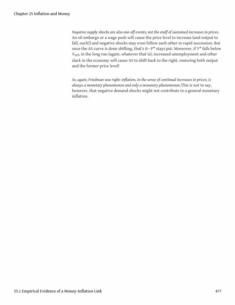
Negative supply shocks are also one-off events, not the stuff of sustained increases in prices.An oil embargo or a wage push will cause the price level to increase (and output tofall, ouch!) and negative shocks may even follow each other in rapid succession. Butonce the AS curve is done shifting, that’s it—P* stays put. Moreover, if Y* falls belowYnrl, in the long run (again, whatever that is), increased unemployment and other
slack in the economy will cause AS to shift back to the right, restoring both outputand the former price level!
So, again, Friedman was right: inflation, in the sense of continual increases in prices, isalways a monetary phenomenon and only a monetary phenomenon.This is not to say,however, that negative demand shocks might not contribute to a general monetaryinflation.
Chapter 25 Inflation and Money
25.1 Empirical Evidence of a Money-Inflation Link 477
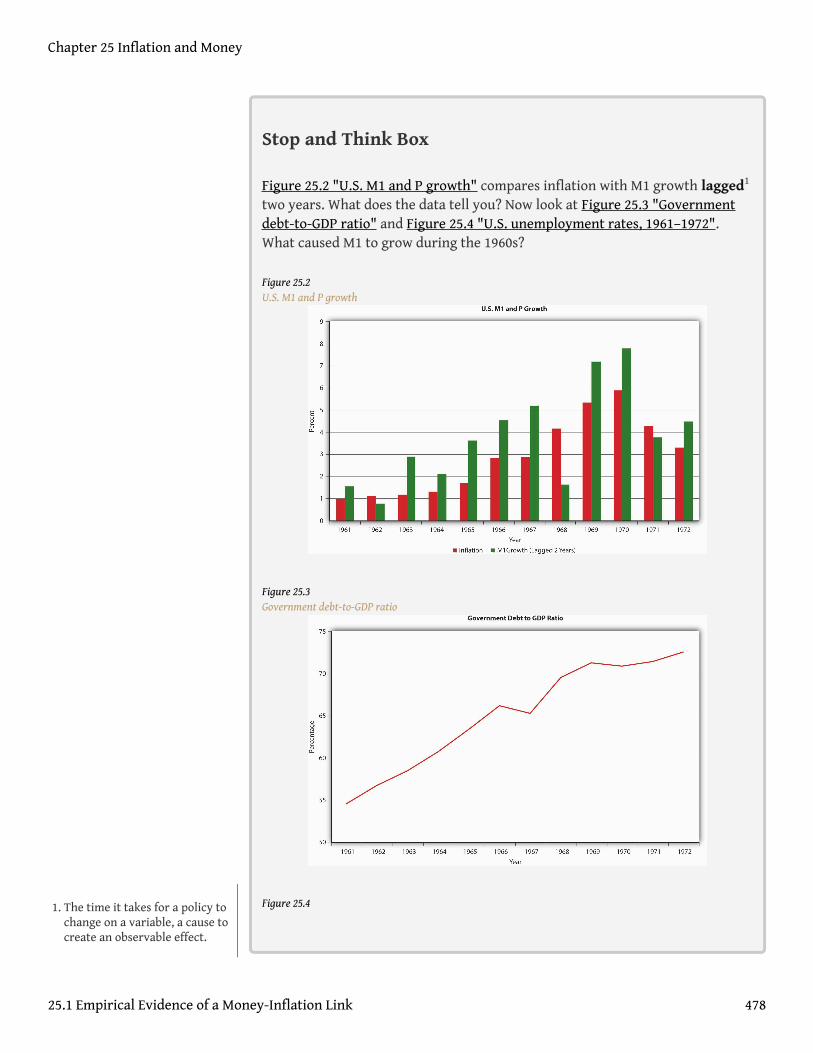
Stop and Think Box
Figure 25.2 "U.S. M1 and P growth" compares inflation with M1 growth lagged1
two years. What does the data tell you? Now look at Figure 25.3 "Governmentdebt-to-GDP ratio" and Figure 25.4 "U.S. unemployment rates, 1961–1972".What caused M1 to grow during the 1960s?
Figure 25.2U.S. M1 and P growth
Figure 25.3Government debt-to-GDP ratio
Figure 25.41. The time it takes for a policy tochange on a variable, a cause tocreate an observable effect.
Chapter 25 Inflation and Money
25.1 Empirical Evidence of a Money-Inflation Link 478
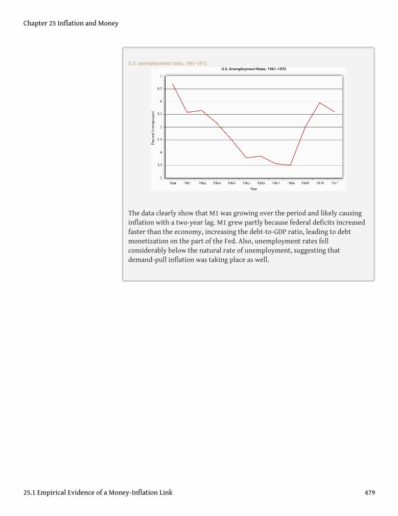
U.S. unemployment rates, 1961–1972
The data clearly show that M1 was growing over the period and likely causinginflation with a two-year lag. M1 grew partly because federal deficits increasedfaster than the economy, increasing the debt-to-GDP ratio, leading to debtmonetization on the part of the Fed. Also, unemployment rates fellconsiderably below the natural rate of unemployment, suggesting thatdemand-pull inflation was taking place as well.
Chapter 25 Inflation and Money
25.1 Empirical Evidence of a Money-Inflation Link 479
KEY TAKEAWAYS
• Throughout history, exogenous increases in MS have led to increases inP*. Every hyperinflation has been preceded by rapid increases in moneysupply growth.
• The AS-AD model shows that money supply growth is the only thing thatcan lead to inflation, that is, sustained increases in the price level.
• This happens because monetary stimulus in the short term shifts the ADcurve to the right, increasing prices but also rendering Y* > Ynrl.
• Unemployment drops, driving up wages, which shifts the AS curve tothe left, Y* back to Ynrl, and P* yet higher.
• Unlike other variables, the MS can continue to grow, initiating roundafter round of this dynamic.
• Other variables are bounded and produce only one-off changes in P*.• A negative supply shock or wage push, for instance, increases the price
level once, but then price increases stop.• Similarly, increases in government expenditures can cause P* to rise by
shifting AD to the right, but unlike increases in the MS, governmentexpenditures can increase only so far politically and practically (to 100percent of GDP).
Chapter 25 Inflation and Money
25.1 Empirical Evidence of a Money-Inflation Link 480
25.2 Why Have Central Bankers So Often Gotten It Wrong?
LEARNING OBJECTIVES
1. Given the analysis in this chapter, why do central bankers sometimesallow inflation to occur year after year?
2. What are lags and why are they important?
If the link between money supply growth and inflation is so clear, and if nobody (exceptperhaps inveterate debtors) has anything but contempt for inflation, why have centralbankers allowed it to occur so frequently? Central bankers might be more privatelyinterested than publicly interested and somehow benefit personally from inflation.(They might score points with politicians for stimulating the economy just beforean election or they might take out big loans and repay them after the inflationaryperiod in nearly worthless currency.) Assuming central bankers are publiclyinterested but far from prescient, what might cause them to err so often? In short,lags and high-employment policies.
A lag is an amount of time that passes between a cause and its eventual effect. Lagsin monetary policy, Friedman showed, were “long and variable.” Data lag is thetime it takes for policymakers to get important information, like GDP (Y) andunemployment. Recognition lag is the time it takes them to become convinced thatthe data is accurate and indicative of a trend and not just a random perturbation.Legislative lag is the time it takes legislators to react to economic changes. (This isshort for monetary policy, but it can be a year or more for fiscal policy.)Implementation lag refers to the time between policy decision and implementation.(Again, for modern central banks using open market purchases (OMPs), this lag isminimal, but for changes in taxes, it can take a long time indeed.) The mostimportant lag of all is the so-called effectiveness lag, the period between policyimplementation and real-world results. All told, lags can add up to years and addconsiderable complexity to monetary policy analysis because they cloud cause-effect relationships. Lags also put policymakers perpetually behind the eight-ball,constantly playing catch-up. Lags force policymakers to forecast the future withaccuracy, something (as we’ve seen) that is not easily done. As noted in earlierchapters, economists don’t even know when the short run becomes the long run!
Consider a case of so-called cost-push inflation brought about by a negative supplyshock or wage push. That moves the AS curve to the left, reducing output andraising prices and, in all likelihood, causing unemployment and political angst.
Chapter 25 Inflation and Money
481
Policymakers unable to await the long term (the rightward shift in AS because Y*has fallen below Ynrl, causing unemployment and wages to decline) may well
respond with what’s called accommodative monetary policy. In other words, theyengage in expansionary monetary policies (EMPs), which shift the AD curve to theright, causing output to increase (with a lag) but prices to rise. Because prices arehigher and they’ve been recently rewarded for their wage push with accommodativemonetary policy, workers may well initiate another wage push, starting a vicious cycle ofwage pushes followed by increases in P* and yet more wage pushes. Monetarists and othernonactivists shake their heads at this dynamic, arguing that if workers’ wagepushes were met by periods of higher unemployment, they would soon learn tostop. (After all, even 2-year-olds and rats eventually learn to stop pushing buttons ifthey are not rewarded for doing so. They learn even faster to stop pushing if theyget a little shock.)
An episode of demand-pull inflation can also touch off accommodative monetary policy anda bout of inflation. If the government sets its full employment target too high, abovethe natural rate, it will always look like there is too much unemployment. That willeventually tempt policymakers into thinking that Y* is < Ynrl, inducing them to
implement an EMP. Output will rise, temporarily, but so too will prices. Prices willgo up again when the AS curve shifts left, back to Ynrl, as it will do in a hurry given
the low level of unemployment. The shift, however, will again increaseunemployment over the government’s unreasonably low target, inducing anotherround of EMP and price increases.
Another source of inflation is government budget deficits. To cover their expenditures,governments can tax, borrow at interest, or borrow for free by issuing money.(Which would you choose?) Taxation is politically costly. Borrowing at interest canbe costly too, especially if the government is a default risk. Therefore, manygovernments pay their bills by printing money or by issuing bonds that theirrespective central banks then buy with money. Either way, the monetary baseincreases, leading to some multiple increases in the MS, which leads to inflation.Effectively a tax on money balances called a currency tax, inflation is easier todisguise and much easier to collect than other forms of taxes. Governments get asaddicted to the currency tax as individuals get addicted to crack or meth. This isespecially true in developing countries with weak (not independent) central banks.
Chapter 25 Inflation and Money
25.2 Why Have Central Bankers So Often Gotten It Wrong? 482
Stop and Think Box
Why is central bank independence important in keeping inflation at bay?
Independent central banks are better able to withstand political pressures tomonetize the debt, to follow accommodative policies, or to respond to(seemingly) “high” levels of unemployment with an EMP. They can also make amore believable or credible commitment to stop inflation, which (as we’ll see inChapter 26 "Rational Expectations Redux: Monetary Policy Implications") is animportant consideration as well.
Chapter 25 Inflation and Money
25.2 Why Have Central Bankers So Often Gotten It Wrong? 483
KEY TAKEAWAYS
• Private-interest scenarios aside, publicly interested central bankersmight pursue high employment too vigorously, leading to inflation viacost-push and demand-pull mechanisms.
• If workers make a successful wage push, for example, the AS curve willshift left, increasing P*, decreasing Y*, and increasing unemployment.
• If policymakers are anxious to get out of recession, they might respondwith an expansionary monetary policy (EMP).
• That will increase Y* but also P* yet again. Such an accommodativepolicy might induce workers to try another wage push. The price level ishigher after all, and they were rewarded for their last wage push.
• The longer this dynamic occurs, the higher prices will go.• Policymakers might fall into this trap themselves if they underestimate
full employment at, say, 97 percent (3 percent unemployment) when infact it is 95 percent (5 percent unemployment).
• Therefore, unemployment of 4 percent looks too high and outputappears to be < Ynrl, suggesting that an EMP is in order.
• The rightward shift of the AD curve causes prices and output to rise, butthe latter rises only temporarily as the already tight labor market getstighter, leading to higher wages and a leftward shift of the AS curve,with its concomitant increase in P* and decrease in Y*.
• If policymakers’ original and flawed estimate of full employment ismaintained, another round of AD is sure to come, as is higher prices.
• Budget deficits can also lead to sustained inflation if the governmentmonetizes its debt directly by printing money (and deposits) orindirectly via central bank open market purchases (OMPs) ofgovernment bonds.
• Lags are the amount of time it takes between a change in the economyto take place and policymakers to effectively do something about it.
• That includes lags for gathering data, making sure the data show a trendand are not mere noise, making a legislative decision (if applicable),implementing policy (if applicable), and waiting for the policy to affectthe economy.
• Lags are important because they are long and variable, thuscomplicating monetary policy by making central bankers play constantcatch-up and also by clouding cause-effect relationships.
Chapter 25 Inflation and Money
25.2 Why Have Central Bankers So Often Gotten It Wrong? 484

25.3 Suggested Reading
Ball, R. J. Inflation and the Theory of Money. Piscataway, NJ: Aldine Transaction, 2007.
Bresciani-Turroni, Costantino. Economics of Inflation. Auburn, AL: Ludwig von MisesInstitute, 2007.
Samuelson, Robert. The Great Inflation and Its Aftermath: The Past and Future ofAmerican Affluence. New York: Random House, 2008.
Chapter 25 Inflation and Money
485
Chapter 26
Rational Expectations Redux: Monetary Policy Implications
CHAPTER OBJECTIVES
By the end of this chapter, students should be able to:
1. Describe how the new classical macroeconomic model differs from thestandard, pre-Lucas AS-AD model.
2. Explain what the new classical macroeconomic model suggestsregarding the efficacy of activist monetary policy.
3. Explain how the new Keynesian model differs from the new classicalmacroeconomic model.
4. Assess the extent to which policymakers can improve short-runmacroeconomic performance.
486
26.1 Rational Expectations
LEARNING OBJECTIVES
1. How does the new classical macroeconomic model differ from thestandard, pre-Lucas AS-AD model?
2. What does the new classical macroeconomic model suggest regardingthe efficacy of activist monetary policy? Why?
It turns out that the theory of rational expectations we learned about in Chapter 7"Rational Expectations, Efficient Markets, and the Valuation of Corporate Equities"has important implications for monetary policy. In a quest to understand whypolicymakers had such a poor record, especially during the 1970s, Len Mirman(University of Virginia),http://www.virginia.edu/economics/mirman.htm RobertLucas (University of Chicago),http://home.uchicago.edu/~sogrodow/ ThomasSargent (New York University),http://homepages.nyu.edu/~ts43/ BennettMcCallum (Carnegie-Mellon),http://public.tepper.cmu.edu/facultydirectory/FacultyDirectoryProfile.aspx?ID=96 Edward Prescott (ArizonaState),http://www.minneapolisfed.org/research/prescott/ and other economists ofthe so-called expectations revolution discovered that expansionary monetary policies cannotbe effective if economic agents expect them to be implemented. Conversely, to thwartinflation as quickly and painlessly as possible, the central bank must be able tomake a credible commitment to stop it. In other words, it must convince peoplethat it can and will stop prices from rising.
Chapter 26 Rational Expectations Redux: Monetary Policy Implications
487
Stop and Think Box
During the American Revolution, the Continental Congress announced that itwould stop printing bills of credit, the major form of money in the economysince 1775–1776, when rebel governments (the Continental Congress and stategovernments) began financing their little revolution by printing money. TheContinental Congress implemented no other policy changes, so everyone knewthat its large budget deficits would continue. Prices continued upward. Why?
The Continental Congress did not make a credible commitment to end inflationbecause its announcement did nothing to end its large and chronic budgetdeficit. It also did nothing to prevent the states from issuing more bills ofcredit.
Lucas was among the first to highlight the importance of public expectations inmacroeconomic forecasting and policymaking. What matters, he argued, was notwhat policymakers’ models said would happen but what economic agents (people,firms, governments) believed would occur. So in one instance, a rise in the fed fundsrate might cause long-term interest rates to barely budge, but in another it mightcause them to soar. In short, policymakers can’t be certain of the effects of their policiesbefore implementing them.
Because Keynesian cross diagrams and the IS-LM and AS-AD models did notexplicitly take rational expectations into account, Lucas, Sargent, and others had torecast them in what is generally called the new classical macroeconomic model.That new model uses the AS, ASL, and AD curves but reduces the short run to zero if thepolicy is expected. So, for example, an anticipated EMP shifts AD right butimmediately shifts AS left as workers spontaneously push for higher wages. Theprice level rises, but output doesn’t budge. An unanticipated EMP, by contrast, has thesame effect as described in earlier chapters—a temporary (but who knows how long?)increase in output (and a rise in P followed by another when the AS curve eventually shiftsleft).
Now get this: Y* can actually decline if an EMP is not as expansionary as expected! Ifeconomic actors expect a big shift in AD, the AS curve will shift hard left to keep Y*at Ynrl, as in Figure 26.1 "The effect of an unexpectedly weak EMP". If the AD curve
does not shift as far right as expected, or indeed if it stays put, prices will rise andoutput will fall, as in the following graph. This helps to explain why financial markets
Chapter 26 Rational Expectations Redux: Monetary Policy Implications
26.1 Rational Expectations 488
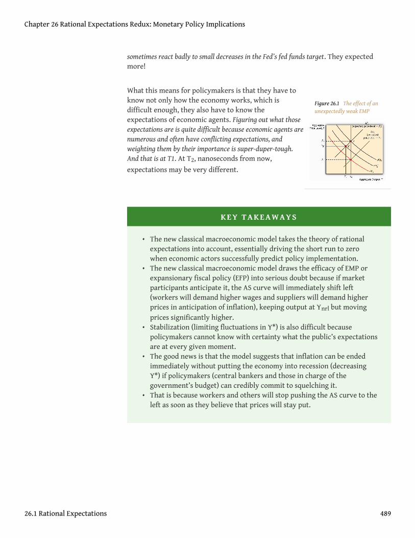
Figure 26.1 The effect of anunexpectedly weak EMP
sometimes react badly to small decreases in the Fed’s fed funds target. They expectedmore!
What this means for policymakers is that they have toknow not only how the economy works, which isdifficult enough, they also have to know theexpectations of economic agents. Figuring out what thoseexpectations are is quite difficult because economic agents arenumerous and often have conflicting expectations, andweighting them by their importance is super-duper-tough.And that is at T1. At T2, nanoseconds from now,
expectations may be very different.
KEY TAKEAWAYS
• The new classical macroeconomic model takes the theory of rationalexpectations into account, essentially driving the short run to zerowhen economic actors successfully predict policy implementation.
• The new classical macroeconomic model draws the efficacy of EMP orexpansionary fiscal policy (EFP) into serious doubt because if marketparticipants anticipate it, the AS curve will immediately shift left(workers will demand higher wages and suppliers will demand higherprices in anticipation of inflation), keeping output at Ynrl but movingprices significantly higher.
• Stabilization (limiting fluctuations in Y*) is also difficult becausepolicymakers cannot know with certainty what the public’s expectationsare at every given moment.
• The good news is that the model suggests that inflation can be endedimmediately without putting the economy into recession (decreasingY*) if policymakers (central bankers and those in charge of thegovernment’s budget) can credibly commit to squelching it.
• That is because workers and others will stop pushing the AS curve to theleft as soon as they believe that prices will stay put.
Chapter 26 Rational Expectations Redux: Monetary Policy Implications
26.1 Rational Expectations 489
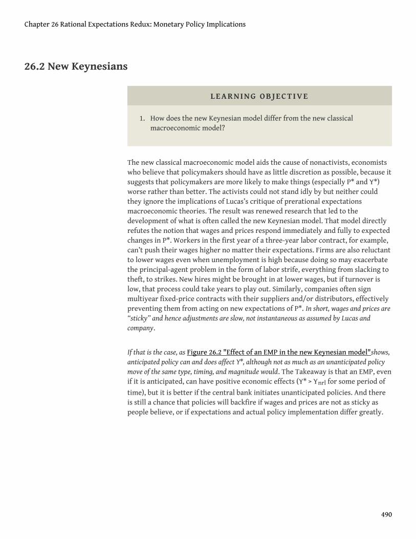
26.2 New Keynesians
LEARNING OBJECTIVE
1. How does the new Keynesian model differ from the new classicalmacroeconomic model?
The new classical macroeconomic model aids the cause of nonactivists, economistswho believe that policymakers should have as little discretion as possible, because itsuggests that policymakers are more likely to make things (especially P* and Y*)worse rather than better. The activists could not stand idly by but neither couldthey ignore the implications of Lucas’s critique of prerational expectationsmacroeconomic theories. The result was renewed research that led to thedevelopment of what is often called the new Keynesian model. That model directlyrefutes the notion that wages and prices respond immediately and fully to expectedchanges in P*. Workers in the first year of a three-year labor contract, for example,can’t push their wages higher no matter their expectations. Firms are also reluctantto lower wages even when unemployment is high because doing so may exacerbatethe principal-agent problem in the form of labor strife, everything from slacking totheft, to strikes. New hires might be brought in at lower wages, but if turnover islow, that process could take years to play out. Similarly, companies often signmultiyear fixed-price contracts with their suppliers and/or distributors, effectivelypreventing them from acting on new expectations of P*. In short, wages and prices are“sticky” and hence adjustments are slow, not instantaneous as assumed by Lucas andcompany.
If that is the case, as Figure 26.2 "Effect of an EMP in the new Keynesian model"shows,anticipated policy can and does affect Y*, although not as much as an unanticipated policymove of the same type, timing, and magnitude would. The Takeaway is that an EMP, evenif it is anticipated, can have positive economic effects (Y* > Ynrl for some period of
time), but it is better if the central bank initiates unanticipated policies. And thereis still a chance that policies will backfire if wages and prices are not as sticky aspeople believe, or if expectations and actual policy implementation differ greatly.
Chapter 26 Rational Expectations Redux: Monetary Policy Implications
490
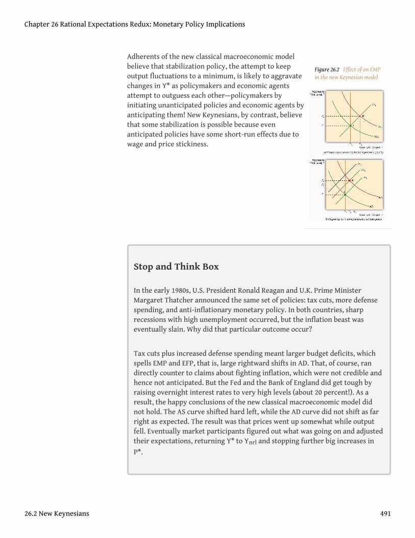
Figure 26.2 Effect of an EMPin the new Keynesian model
Adherents of the new classical macroeconomic modelbelieve that stabilization policy, the attempt to keepoutput fluctuations to a minimum, is likely to aggravatechanges in Y* as policymakers and economic agentsattempt to outguess each other—policymakers byinitiating unanticipated policies and economic agents byanticipating them! New Keynesians, by contrast, believethat some stabilization is possible because evenanticipated policies have some short-run effects due towage and price stickiness.
Stop and Think Box
In the early 1980s, U.S. President Ronald Reagan and U.K. Prime MinisterMargaret Thatcher announced the same set of policies: tax cuts, more defensespending, and anti-inflationary monetary policy. In both countries, sharprecessions with high unemployment occurred, but the inflation beast waseventually slain. Why did that particular outcome occur?
Tax cuts plus increased defense spending meant larger budget deficits, whichspells EMP and EFP, that is, large rightward shifts in AD. That, of course, randirectly counter to claims about fighting inflation, which were not credible andhence not anticipated. But the Fed and the Bank of England did get tough byraising overnight interest rates to very high levels (about 20 percent!). As aresult, the happy conclusions of the new classical macroeconomic model didnot hold. The AS curve shifted hard left, while the AD curve did not shift as farright as expected. The result was that prices went up somewhat while outputfell. Eventually market participants figured out what was going on and adjustedtheir expectations, returning Y* to Ynrl and stopping further big increases in
P*.
Chapter 26 Rational Expectations Redux: Monetary Policy Implications
26.2 New Keynesians 491
KEY TAKEAWAYS
• The new Keynesian model leaves more room for discretionary monetarypolicy.
• Like the new classical macroeconomic model, it is post-Lucas and hencerealizes that expectations are important to policy outcomes.
• Unlike the new classical macroeconomic model, however, it positssignificant wage and price stickiness (basically long-term contracts) thatprevents the AS curve from shifting immediately and completely,regardless of the expectations of economic actors.
• EMP (and EFP) can therefore increase Y* over Ynrl, although less than ifthe policy were unanticipated (although, of course, at the cost of higherP*; the long-term analysis of the AS-AD model still holds). Similarly, tothe extent that wages and prices are sticky, some stabilization ispossible because policymakers can count on some output response totheir policies.
• The new Keynesian model is more pessimistic about curbing inflation,however, because the stickiness of the AS curve prevents prices andwages from completely and instantaneously adjusting to a crediblecommitment.
• Output losses, however, will be smaller than an unanticipated move tosquelch inflation. Some economists think it is possible to minimize theoutput losses further by essentially reducing the stickiness of the AS bycredibly committing to slowly reducing inflation.
Chapter 26 Rational Expectations Redux: Monetary Policy Implications
26.2 New Keynesians 492
26.3 Inflation Busting
LEARNING OBJECTIVE
1. Can policymakers improve short-run macroeconomic performance? Ifso, how?
FIX FIGURE Fighting inflation requires the central bank to hold the line on AD, evenin the face of a leftward shift in the AS curve that causes a recession (Y* < Ynrl). The
question is, How much will fighting inflation “cost” the economy in terms of lost output?According to the pre-Lucas AS-AD model, about 4 percent per year for each 1 percent shavedfrom inflation! The new classical macroeconomic model, by contrast, is much moreoptimistic. If the public knows and believes that the central bank will fight inflation,output won’t fall at all because both the AD and the AS curves will stay put. Workerswon’t fight for higher wages because they expect P* will stay the same. Anunanticipated anti-inflation stance, by contrast, will cause a recession. The moral ofthe story told by the new classical macroeconomic model appears to be that the central bankshould be very transparent about fighting inflation but opaque about EMP!
The new Keynesian model also concludes that an unanticipated anti-inflation policyis worse than an anticipated and credible one, though it suggests that some drop inY* should be expected due to stickiness. A possible solution to that problem is toslowly ease money supply growth rather than slamming the brakes on. If theslowing is expected and credible (in other words, if economic agents know theslowing is coming and fully expect it to continue until inflation is history), the AScurve can be “destickyfied” to some degree. Maybe contracts indexed to inflationwill expire and not be renewed, new contracts will build in no or at least lowerinflation expectations, or perhaps contracts (for materials or labor) will becomeshorter term. If that is the case, when money supply growth finally stops,something akin to the unsticky world of the new classical macroeconomic modelwill hold; the AS curve won’t shift much, if at all; and inflation will cease without amajor drop in output.
How can central bankers increase their credibility? One way is to make their centralbanks more independent. Another is not to repeatedly announce A but do B. A thirdis to induce the government to decrease or eliminate budget deficits.
Chapter 26 Rational Expectations Redux: Monetary Policy Implications
493
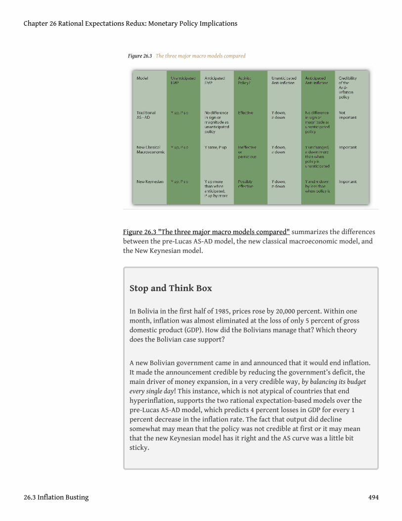
Figure 26.3 The three major macro models compared
Figure 26.3 "The three major macro models compared" summarizes the differencesbetween the pre-Lucas AS-AD model, the new classical macroeconomic model, andthe New Keynesian model.
Stop and Think Box
In Bolivia in the first half of 1985, prices rose by 20,000 percent. Within onemonth, inflation was almost eliminated at the loss of only 5 percent of grossdomestic product (GDP). How did the Bolivians manage that? Which theorydoes the Bolivian case support?
A new Bolivian government came in and announced that it would end inflation.It made the announcement credible by reducing the government’s deficit, themain driver of money expansion, in a very credible way, by balancing its budgetevery single day! This instance, which is not atypical of countries that endhyperinflation, supports the two rational expectation-based models over thepre-Lucas AS-AD model, which predicts 4 percent losses in GDP for every 1percent decrease in the inflation rate. The fact that output did declinesomewhat may mean that the policy was not credible at first or it may meanthat the new Keynesian model has it right and the AS curve was a little bitsticky.
Chapter 26 Rational Expectations Redux: Monetary Policy Implications
26.3 Inflation Busting 494
KEY TAKEAWAYS
• Whether policymakers can improve short-term macroeconomicperformance depends on the degree of wage and price stickiness, that is,how much more realistic the new Keynesian model is than the newclassical macroeconomic model.
• If the latter is correct, any attempts at EMP and EFP that are anticipatedby economic actors will fail to raise Y* and, in fact, can reduce Y* if thestimulus is less than the public expected. The only hope is to implementunanticipated policies, but that is difficult to do because central bankerscan never be absolutely sure what expectations are at the time of policyimplementation.
• On the other hand, inflation can be squelched relatively easily by simplyannouncing the policy and taking steps to ensure its credibility.
• If the new Keynesian model is correct, Y* can be increased over Ynrl (inthe short term only, of course) because, regardless of expectations,wages and prices cannot rise due to multiyear contractual commitmentslike labor union contracts and other sources of stickiness.
• Inflation can also be successfully fought by announcing a credible policy,but due to wage and price stickiness, it will take a little time to take holdand output will dip below Ynrl, though by much less than the pre-LucasAS-AD model predicts.
Chapter 26 Rational Expectations Redux: Monetary Policy Implications
26.3 Inflation Busting 495
26.4 Suggested Reading
Gali, Jordi. Monetary Policy, Inflation, and the Business Cycle: An Introduction to the NewKeynesian Framework. Princeton, NJ: Princeton University Press, 2008.
Lucas, Robert, and Thomas Sargent. Rational Expectations and Econometric Practice.Minneapolis: University of Minnesota Press, 1981.
Scheffrin, Steven. Rational Expectations. New York: Cambridge University Press, 1996.
Chapter 26 Rational Expectations Redux: Monetary Policy Implications
496