Financial Crises, Bank Risk Exposureand

Government Financial Policy�

Mark Gertler, Nobuhiro Kiyotaki, and Albert Queralto

N.Y.U. and Princeton

September 2010(this version) May 2011

Abstract

A macroeconomic model with �nancial intermediation is developed in which theintermediaries (banks) can issue outside equity as well as short term debt. This makesbank risk exposure an endogenous choice. The goal is to have a model that can notonly capture a crisis when banks are highly vulnerable to risk, but can also accountfor why banks adopt such a risky balance sheet in the �rst place. We use the modelto assess quantitatively how perceptions of fundamental risk and of government creditpolicy in a crisis a¤ect the vulnerability of the �nancial system ex ante. We also studythe e¤ects of macro-prudential policies designed to o¤set the incentives for risk-taking.

�We thank Philippe Bacchetta and Elu Von Thadden for helpful comments. Gertler and Kiyotaki alsowish to acknoweldge the support of the NSF.

1

1 Introduction

A distinguishing feature of the recent U.S. recession - known now as the Great Recession- was the signi�cant disruption of �nancial intermediation. The meltdown of the shadowbanking system along with the associated strain placed on the entire �nancial system led toan extraordinary increase in �nancing costs. This increase in �nancing costs, which peakedin the wake of the Lehman Brothers collapse, is considered a major factor in the collapseof durable goods spending in the fall of 2008 that in turn triggered the huge contraction inoutput and employment.The challenge for macroeconomists has been to build models that can not only capture

this phenomenon but also be used to analyze the variety of unconventional measures pursuedby the monetary and the �scal authorities to stabilize credit markets. In this regard, therehas been a rapidly growing literature that attempts to incorporate �nancial factors withinthe quantitative macroeconomic frameworks that had been the workhorses for monetaryand �scal policy analysis up until this point. Much of this work is surveyed in Gertler andKiyotaki (2010). A common feature of many of these papers has been to extend the basic�nancial accelerator mechanism developed by Bernanke and Gertler (1989) and Kiyotakiand Moore (1997) to �nancial intermediaries (�banks�) in order to capture the disruption ofintermediation.Key to motivating a crisis within these frameworks is the heavy reliance of banks on

short term debt. This feature makes these institutions highly exposed to the risk of adversereturns to their balance sheet in way that is consistent with recent experience. Within theseframeworks and most others in this class, however, by assumption the only way banks canobtain external funds is by issuing short term debt.1 Thus, in their present form, these modelsare not equipped to address how the �nancial system found itself so vulnerable in the �rstplace. This question is of critical importance for designing policies to ensure the economydoes not wind up in this position again. For example, a number of authors have suggestedthat such a risky bank liability structure was ultimately the product of expectations thegovernment will intervene to stabilize �nancial markets in a crisis, just as it did recently.With the existing macroeconomic frameworks it is not possible to address this issue.In this paper we develop a macroeconomic model with an intermediation sector that al-

lows banks to issue outside equity as well as short term debt. This makes bank risk exposurean endogenous choice. Here the goal is to have a model that can not only capture a crisiswhen �nancial institutions are highly vulnerable to risk, but also account for why these in-stitutions adopt such a risky balance sheet structure in the �rst place. The basic frameworkbuilds on Gertler and Karadi (2011) and Gertler and Kiyotaki (2010). It extends the agencyproblem between banks and savers within these frameworks to allow intermediaries a mean-ingful trade-o¤ between short term debt and equity. Ultimately, a bank�s decision over itsbalance sheet will depend on its perceptions of risk, which will in turn depend on both thefundamental disturbances to the economy and expectations about government policy.We �rst use the model to analyze how di¤erent degrees of fundamental risk in the econ-

1Some quantitative macro models with �nancial sectors include: Bernanke, Gertler and Gilchrist (1999),Brunnermeier and Sannikov (2009), Christiano, Motto and Rostagno (2009), Gilchrist, Ortiz and Zakresjek(2009), Mendoza (2010) and Jermann and Quadrini (2009). Only the latter considers both debt and equity�nance, though they restrict attention to borrowing constraints faced by non-�nancial �rms.

2

omy a¤ect the balance sheet structure of banks and the aggregate equilibrium. We thenanalyze the vulnerability of the economy to a crisis in each kind of risk environment. Whenperceptions of risk are low, banks opt for greater leverage. But this has the e¤ect of makingthe economy more vulnerable to a crisis.We next turn to analyzing credit policy during a crisis. Following Gertler and Karadi

(2011), we analyze large scale asset purchases of the type the Federal Reserve used to helpstabilize �nancial markets following the Lehman collapse. Within this framework, the centralbank has an advantage during a crisis that it can easily obtain funds by issuing short termgovernment debt, in contrast to private intermediaries that are constrained by the weaknessof their respective balance sheets. Thus this kind of credit policy is e¤ective in mitigating acrisis even if the central bank is less e¢ cient in acquiring assets than is private sector.What is new in the present framework is that it is possible to capture the side e¤ect of the

credit policy on moral hazard. In particular, as we show, the anticipated credit policy willinduce banks to adopt a riskier balance sheet, which will in turn require a larger scale creditmarket intervention during a crisis. This sets the stage for an analysis of macro-prudentialpolicy designed to o¤set the e¤ects of anticipated credit policy on the incentives for bankrisk-taking.To be sure, there is lengthy theoretical literature that examines the sources of vulnera-

bility of a �nancial system. For example, Fostel and Geanakoplos (2009) stress the role ofinvestor optimism in encouraging risk taking. Others such as Diamond and Rajan (2009),Fahri and Tirole (2009) and Chari and Kehoe (2009) stress moral hazard consequences ofbailouts and other credit market interventions. Our paper di¤ers mainly by couching theanalysis within a full blown macroeconomic model to provide a step toward assessing thequantitative implications.There is as well a related literature that analyzes macro-prudential policy. Again, much

of it is qualitative (e.g. Lorenzoni, 2009, Korinek, 2009, and Stein 2010). However, thereare also quantitative frameworks, e.g., Bianchi (2009) and Nikolov (2009). Our frameworkdi¤ers partly by endogenizing the �nancial friction and partly by exploring the interactionbetween credit policies used to stabilize the economy ex post and macro-prudential policyused to mitigate risk taking ex ante.Finally relevant are the literatures on international risk sharing and on asset pricing

and business cycles.2 Conventional quantitative models used for policy evaluation typicallyexamine linear dynamics within a local neighborhood of a deterministic steady state. Indoing so they abstract from an explicit consideration of uncertainty. Because bank liabilitystructure will depend on perceptions of risk, however, accounting for uncertainty is critical.Here we borrow insights from these literatures by considering second order approximationsto pin down determinate bank liability shares.

2See, for example, Campbell (1994), Devereux and Sutherland (2009), Lettau (2003) and Tille and VanWincoop (2007).

3

2 The Baseline Model

2.1 Physical Setup

Before introducing �nancial frictions, we present the basic physical environment. There area continuum of �rms of mass of unity. Each �rm produces output using an identical constantreturns to scale Cobb-Douglas production function with capital and labor as inputs. We canexpress aggregate output Yt as a function of aggregate capital Kt and aggregate labor hoursLt as:

Yt = AtKt�L1��t ; 0 < � < 1; (1)

where At is aggregate productivity which follows a stationary Markov process.Let St be the aggregate capital stock �in process�for period t + 1 . Capital in process

at t for t + 1 is the sum of current investment It and the stock of undepreciated capital,(1� �)Kt:

St = (1� �)Kt + It: (2)

Capital in process for period t + 1 is transformed into capital for production after the real-ization of a multiplicative shock to capital quality, t+1;

Kt+1 = t+1St: (3)

Following the �nance literature (e.g., Merton (1973)), we introduce the capital quality shockas a simple way to introduce an exogenous source of variation in the value of capital. As willbecome clear later, the market price of capital will be endogenous within our framework.In this regard, the capital quality shock will serve as an exogenous trigger of asset pricedynamics. The random variable t+1 is best thought of as capturing some form of economicobsolescence, as opposed to physical depreciation. Appendix B in the working paper versionof this paper provides an explicit micro-foundation. We assume the capital quality shock t+1 follows an i.i.d. process, with an unconditional mean of unity. In addition, we allowfor occasional disasters in the form of sharp contractions in quality, as describe later. Thesedisaster shocks serve to instigate �nancial crises.3

Firms acquire new capital from capital goods producers. There are convex adjustmentcosts in the rate of change in investment goods output for capital goods producers. Ag-gregate output is divided between household consumption Ct, investment expenditures, andgovernment consumption Gt,

Yt = Ct + [1 + f(ItIt�1

)]It +Gt; (4)

where f( ItIt�1)It re�ects physical adjustment costs, with f(1) = f 0(1) = 0 and f 00(It=It�1) > 0.

3Other recent papers that make use of this kind of disturbance include, Gertler and Karadi (2011),Brunnermeier and Sannikov (2009) and Gourio (2009). An alternative but more cumbersome approachwould be to introduce a "news" shock that a¤ects current asset values. Gertler and Karadi (2011) illustratethe similarities between the two.

4

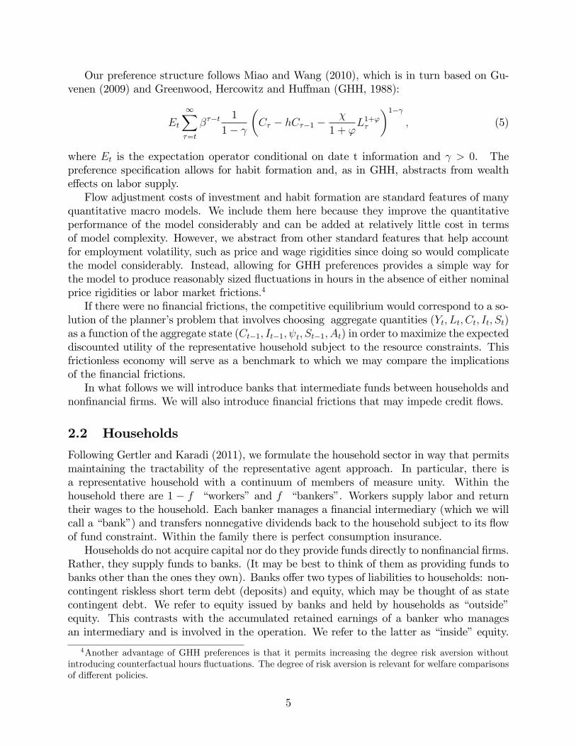
Our preference structure follows Miao and Wang (2010), which is in turn based on Gu-venen (2009) and Greenwood, Hercowitz and Hu¤man (GHH, 1988):

Et

1X�=t

���t1

1�

�C� � hC��1 �

�

1 + 'L1+'�

�1� ; (5)

where Et is the expectation operator conditional on date t information and > 0. Thepreference speci�cation allows for habit formation and, as in GHH, abstracts from wealthe¤ects on labor supply.Flow adjustment costs of investment and habit formation are standard features of many

quantitative macro models. We include them here because they improve the quantitativeperformance of the model considerably and can be added at relatively little cost in termsof model complexity. However, we abstract from other standard features that help accountfor employment volatility, such as price and wage rigidities since doing so would complicatethe model considerably. Instead, allowing for GHH preferences provides a simple way forthe model to produce reasonably sized �uctuations in hours in the absence of either nominalprice rigidities or labor market frictions.4

If there were no �nancial frictions, the competitive equilibrium would correspond to a so-lution of the planner�s problem that involves choosing aggregate quantities (Yt; Lt; Ct; It; St)as a function of the aggregate state (Ct�1; It�1; t; St�1; At) in order to maximize the expecteddiscounted utility of the representative household subject to the resource constraints. Thisfrictionless economy will serve as a benchmark to which we may compare the implicationsof the �nancial frictions.In what follows we will introduce banks that intermediate funds between households and

non�nancial �rms. We will also introduce �nancial frictions that may impede credit �ows.

2.2 Households

Following Gertler and Karadi (2011), we formulate the household sector in way that permitsmaintaining the tractability of the representative agent approach. In particular, there isa representative household with a continuum of members of measure unity. Within thehousehold there are 1 � f �workers�and f �bankers�. Workers supply labor and returntheir wages to the household. Each banker manages a �nancial intermediary (which we willcall a �bank�) and transfers nonnegative dividends back to the household subject to its �owof fund constraint. Within the family there is perfect consumption insurance.Households do not acquire capital nor do they provide funds directly to non�nancial �rms.

Rather, they supply funds to banks. (It may be best to think of them as providing funds tobanks other than the ones they own). Banks o¤er two types of liabilities to households: non-contingent riskless short term debt (deposits) and equity, which may be thought of as statecontingent debt. We refer to equity issued by banks and held by households as �outside�equity. This contrasts with the accumulated retained earnings of a banker who managesan intermediary and is involved in the operation. We refer to the latter as �inside�equity.

4Another advantage of GHH preferences is that it permits increasing the degree risk aversion withoutintroducing counterfactual hours �uctuations. The degree of risk aversion is relevant for welfare comparisonsof di¤erent policies.

5

The distinction between outside and inside equity will become important later since bankswill face constraints in obtaining external funds. In addition, households may acquire shortterm riskless government debt. Both bank deposits and government debt are one periodreal riskless bonds and thus are perfect substitute in the equilibrium we consider. Thus weimpose this condition from the onset and assume that both pay the same gross real returnRt from t� 1 to t:We normalize the units of outside equity so that each equity is a claim to the future returns

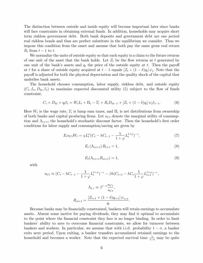
of one unit of the asset that the bank holds. Let Zt be the �ow returns at t generated byone unit of the bank�s assets and qt the price of the outside equity at t. Then the payo¤at t for a share of outside equity acquired at t � 1 equals [Zt + (1� �)qt] t: Note that thepayo¤ is adjusted for both the physical depreciation and the quality shock of the capital thatunderlies bank assets.The household chooses consumption, labor supply, riskless debt, and outside equity

(Ct; Lt; Dht; et) to maximize expected discounted utility (5) subject to the �ow of fundsconstraint,

Ct +Dht + qtet = WtLt +�t � Tt +RtDht�1 + [Zt + (1� �)qt] tet�1: (6)

Here Wt is the wage rate, Tt is lump sum taxes, and �t is net distributions from ownershipof both banks and capital producing �rms. Let uCt denote the marginal utility of consump-tion and �t;t+1 the household�s stochastic discount factor. Then the household�s �rst orderconditions for labor supply and consumption/saving are given by

EtuCtWt = �L't (Ct � hCt�1 ��

1 + 'L1+'t )� ; (7)

Et (�t;t+1)Rt+1 = 1; (8)

Et(�t;t+1Ret+1) = 1; (9)

with

uCt � (Ct � hCt�1 ��

1 + 'L1+'t )� � �h(Ct+1 � hCt

�

1 + 'L1+'t+1 )

� ;

�t;� � ���tuC�uCt

;

Ret+1 =[Zt+1 + (1� �)qt+1] t+1

qt:

Because banks may be �nancially constrained, bankers will retain earnings to accumulateassets. Absent some motive for paying dividends, they may �nd it optimal to accumulateto the point where the �nancial constraint they face is no longer binding. In order to limitbankers� ability to save to overcome �nancial constraints, we allow for turnover betweenbankers and workers. In particular, we assume that with i.i.d. probability 1 � �, a bankerexits next period. Upon exiting, a banker transfers accumulated retained earnings to thehousehold and becomes a worker. Note that the expected survival time 1

1�� may be quite

6

long. It is critical, however, that the expected horizon is �nite, in order to motivate payoutswhile the �nancial constraints are still binding.Each period, (1 � �)f workers randomly become bankers, keeping the number in each

occupation constant. Finally, because in equilibrium bankers will not be able to operatewithout any �nancial resources, each new banker receives a �start up� transfer from thefamily as a small constant fraction of the aggregate assets of bankers.5 Accordingly, �t isnet funds transferred to the household, i.e., funds transferred from exiting bankers minusthe funds transferred to new bankers (aside from pro�ts of capital producers).

2.3 Non�nancial Firms

There are two types of non�nancial �rms: goods producers and capital producers.

2.3.1 Goods Producers

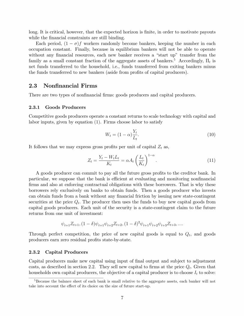
Competitive goods producers operate a constant returns to scale technology with capital andlabor inputs, given by equation (1). Firms choose labor to satisfy

Wt = (1� �)YtLt: (10)

It follows that we may express gross pro�ts per unit of capital Zt as,

Zt =Yt �WtLt

Kt

= �At

�LtKt

�1��: (11)

A goods producer can commit to pay all the future gross pro�ts to the creditor bank. Inparticular, we suppose that the bank is e¢ cient at evaluating and monitoring non�nancial�rms and also at enforcing contractual obligations with these borrowers. That is why theseborrowers rely exclusively on banks to obtain funds. Then a goods producer who investscan obtain funds from a bank without any �nancial friction by issuing new state-contingentsecurities at the price Qt: The producer then uses the funds to buy new capital goods fromcapital goods producers. Each unit of the security is a state-contingent claim to the futurereturns from one unit of investment:

t+1Zt+1; (1� �) t+1 t+2Zt+2; (1� �)2 t+1 t+2 t+3Zt+3; ::::

Through perfect competition, the price of new capital goods is equal to Qt, and goodsproducers earn zero residual pro�ts state-by-state.

2.3.2 Capital Producers

Capital producers make new capital using input of �nal output and subject to adjustmentcosts, as described in section 2.2. They sell new capital to �rms at the price Qt: Given thathouseholds own capital producers, the objective of a capital producer is to choose It to solve:

5Because the balance sheet of each bank is small relative to the aggregate assets, each banker will nottake into account the e¤ect of its choice on the size of future start-up.

7

maxEt

1X�=t

�t;�

�Q�I� �

�1 + f

�I�I��1

��I�

�:

From pro�t maximization, the price of capital goods is equal to the marginal cost of invest-ment goods production as,

Qt = 1 + f

�ItIt�1

�+

ItIt�1

f 0(ItIt�1

)� Et�t;t+1(It+1It)2f 0(

It+1It): (12)

Pro�ts (which arise only outside of steady state), are redistributed lump sum to households.

2.4 Banks

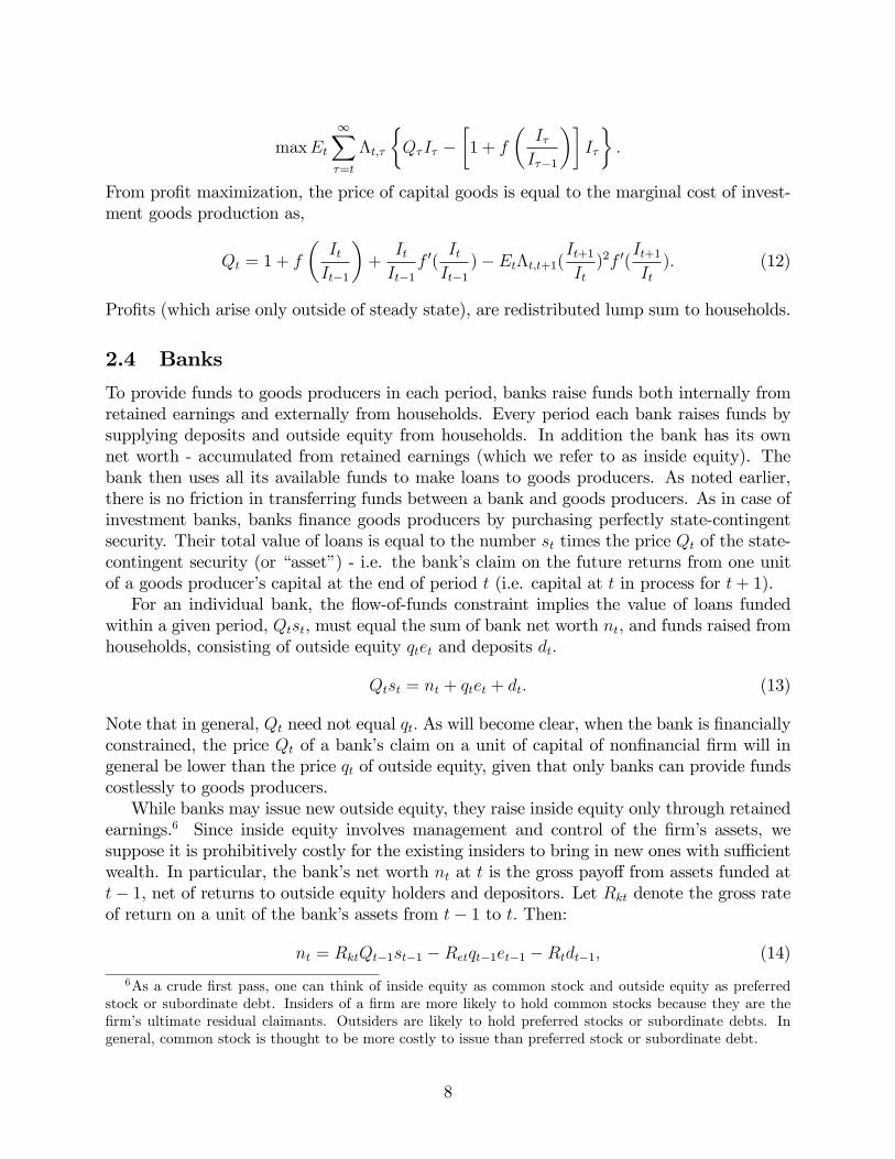
To provide funds to goods producers in each period, banks raise funds both internally fromretained earnings and externally from households. Every period each bank raises funds bysupplying deposits and outside equity from households. In addition the bank has its ownnet worth - accumulated from retained earnings (which we refer to as inside equity). Thebank then uses all its available funds to make loans to goods producers. As noted earlier,there is no friction in transferring funds between a bank and goods producers. As in case ofinvestment banks, banks �nance goods producers by purchasing perfectly state-contingentsecurity. Their total value of loans is equal to the number st times the price Qt of the state-contingent security (or �asset�) - i.e. the bank�s claim on the future returns from one unitof a goods producer�s capital at the end of period t (i.e. capital at t in process for t+ 1).For an individual bank, the �ow-of-funds constraint implies the value of loans funded

within a given period, Qtst, must equal the sum of bank net worth nt, and funds raised fromhouseholds, consisting of outside equity qtet and deposits dt:

Qtst = nt + qtet + dt: (13)

Note that in general, Qt need not equal qt: As will become clear, when the bank is �nanciallyconstrained, the price Qt of a bank�s claim on a unit of capital of non�nancial �rm will ingeneral be lower than the price qt of outside equity, given that only banks can provide fundscostlessly to goods producers.While banks may issue new outside equity, they raise inside equity only through retained

earnings.6 Since inside equity involves management and control of the �rm�s assets, wesuppose it is prohibitively costly for the existing insiders to bring in new ones with su¢ cientwealth. In particular, the bank�s net worth nt at t is the gross payo¤ from assets funded att� 1, net of returns to outside equity holders and depositors. Let Rkt denote the gross rateof return on a unit of the bank�s assets from t� 1 to t: Then:

nt = RktQt�1st�1 �Retqt�1et�1 �Rtdt�1; (14)

6As a crude �rst pass, one can think of inside equity as common stock and outside equity as preferredstock or subordinate debt. Insiders of a �rm are more likely to hold common stocks because they are the�rm�s ultimate residual claimants. Outsiders are likely to hold preferred stocks or subordinate debts. Ingeneral, common stock is thought to be more costly to issue than preferred stock or subordinate debt.

8

with

Rkt =[Zt + (1� �)Qt] t

Qt�1;

and where the rate of return on outside equity Ret is given by equation (9). Observe thatoutside equity permits the bank to hedge against �uctuations in the return on its assets. Itis this hedging value that makes it attractive to the bank to issue outside equity.Given the bank faces a �nancing constraint, it is in its interest to retain all earnings until

the time it exits, at which point it pays out its accumulated retained earnings as dividends.Accordingly, the objective of the bank at the end of period t is the expected present valueof the future terminal dividend,

Vt = Et

" 1X�=t+1

(1� �)���t�1�t;�n�

#: (15)

To motivate an endogenous constraint on the bank�s ability to obtain funds, we introducethe following simple agency problem: We assume that after a bank obtains funds, the bankermanaging the bank may transfer a fraction of assets to his or her family. It is the recognitionof this possibility that has households limit the funds they lend to banks.In addition, we assume that the fraction of funds the bank may divert depends on the

composition of its liabilities. In particular, we assume that at the margin it is more di¢ cultto divert assets funded by short term deposits than by outside equity. Short term depositsrequire the bank to continuously meet a non-contingent payment. Dividend payments, incontrast, are tied to the performance of the bank�s assets, which is di¢ cult for outsidersto monitor. By giving banks less discretion over payouts, short term deposits o¤er morediscipline over bank managers than does outside equity.7

Let xt denote the fraction of bank assets funded by outside equity:

xt =qtetQtst

: (16)

Then we assume that after the bank has obtained funds it may divert the fraction �(xt) ofassets, where �(xt) is the convex function of xt:

�(xt) = ��1 + "xt +

�

2x2t

�: (17)

We allow for the possibility that there could be some e¢ ciency gains in monitoring the bankfrom having at least a bit of outside equity participation in funding the bank (i.e. " can benegative). However, we restrict attention to calibrations where the bank�s ability to divertassets increases when outside equity replaces deposits for funding: at the margin �("+ �xt)is positive. Finally, we assume that the banker�s decision over whether to divert funds mustbe made at the end of the period t but before the realization of aggregate uncertainty in thefollowing period. Here the idea is that if the banker is going to divert funds, it takes timeto position assets and this must be done between the periods (e.g., during the night).

7The idea that short term debt serves as a disciplining devices over banks is due to Calomiris and Kahn(1991).

9

If a bank diverts assets for its personal gain, it defaults on its debt and is shut down.The creditors may re-claim the remaining fraction 1��(xt) of funds. Because its creditorsrecognize the bank�s incentive to divert funds, they will restrict the amount they lend. Inthis way bank may face an external �nancing constraint.Let Vt(st; xt; nt) be the maximized value of the bank�s objective Vt, given an asset and

liability con�guration (st; xt; nt) at the end of period t. Then in order to ensure the bankdoes not divert funds, the incentive constraint must hold:

Vt � �(xt)Qtst: (18)

Equation (18) states that for households to be willing to supply funds to a bank, the bank�sfranchise value Vt must be at least as large as its gain from diverting funds.Combining (13) and (14) yields the evolution of nt as a function of st�1; xt�1 and nt�1 as,

nt = [Rkt � xt�1Ret � (1� xt�1)Rt]Qt�1st�1 +Rtnt�1: (19)

It follows that in general the franchise value of the bank at the end of period t� 1 satis�esthe Bellman equation

Vt�1(st�1; xt�1; nt�1) = Et�1�t�1;tf(1� �)nt + �Maxst;xt:

[Vt(st; xt; nt)]g: (20)

where the right side takes into account that the bank exits with probability 1 � � andcontinues with probability �. Accordingly, at each time t; the bank bank chooses st andxt to maximize Vt(st; xt; nt) subject to the incentive constraint (18) and the law of motionfor net worth (19). We conjecture the value function Vt is the function of the balance sheetcomponents as:

Vt(st; xt; nt) = (�st + xt�et)Qtst + �tnt: (21)

In Appendix A of our companion working paper, we provide a detailed derivations and verifythis conjecture.We begin with the solution for st: Let �t be the maximum ratio of bank assets to net

worth (leverage ratio) that satis�es the incentive constraint. Then by construction,

Qtst = �tnt: (22)

Equation (22) is a key relation of the banking sector: It indicates that when the borrowingconstraint binds, the total quantity of private assets that a bank can intermediate is limitedby its net worth, nt: From the bank�s optimization problem, �t is given by

�t =�t

�(xt)� (�st + xt�et); (23)

with

�t = Et(�t;t+1t+1)Rt+1; (24)

�st = Et[�t;t+1t+1(Rkt+1 �Rt+1)]; (25)

10

�et = Et[�t;t+1t+1(Rt+1 �Ret+1)]: (26)

t+1 is the shadow value of a unit of net worth to the bank at t+ 1 and is given by

t+1 = 1� � + �[�t+1 + �t+1(�st+1 + xt+1�et+1)]: (27)

The relation is intuitive: The leverage ratio �t is increasing in two factors which raise thefranchise value of the bank: the discounted excess value of bank assets (�st + xt�et) and thesaving in deposit costs from another unit of net worth �t: Because both these factors raisethe bank�s franchise value of bank, they reduce the incentive for the bank to divert funds,making its creditors willing to lend more. Conversely, �t is decreasing in �(xt), the fractionof funds banks are able to divert.The leverage ratio also varies inversely with risk perceptions. In particular, the bank

values its expected returns using an �augmented stochastic discount factor,�which is theproduct of the household stochastic discount factor �t;t+1 and the stochastic shadow marginalvalue of net worth t+1: Note that the latter varies countercyclically: because the bank�sincentive constraint is tighter in recessions than in booms, an additional unit of net worth ismore valuable in bad times than in good times. Accordingly, since both t+1 and �t;t+1 arecounter-cyclical, the augmented stochastic discount factor is countercyclical. It follows thatsince the realized excess return to assets Rkt+1�Rt+1 varies procyclically, increased volatilityin the bank�s stochastic discount factor reduces the excess value of the bank�s assets and thusits continuation value: The leverage ratio drops as a result. In this way, uncertainty a¤ectsthe bank�s ability to obtain funds.We next turn to the choice of the liability structure. As we show in our companion

working paper, the fraction of assets �nanced by outside equity, xt, is increasing in the ratioof the excess value from substituting outside equity for deposit �nance (�et) to the excessvalue on assets over the deposit (�st) as follows:

xt = ��st�et

+ [(�st�et)2 +

2

�(1� "

�st�et)]

12 (28)

= x

��et�st

�; where x0 > 0:

The excess value to the bank from outside equity issues arises because the �nancingconstraint e¤ectively makes it more risk averse than households. From (26), �et is theexpected value of the product of the augmented stochastic discount factor and the di¤erencein the rate of returns on deposits and outside equity Rt+1 � Ret+1: On the other hand, thehousehold�s portfolio decision yields the following arbitrage relation between the deposit rateand the return on outside equity:

Et[�t;t+1(Rt+1 �Ret+1)] = 0: (29)

Observe that the household discounts the returns by the stochastic factor �t;t+1 while thebanker uses a discount factor �t;t+1t+1. Since the latter is more volatile and countercyclicalthan the former, the bank obtains hedging value by switching from deposits to outside equity:Accordingly, the excess value of outside equity issue �et = Et[�t;t+1t+1(Rt+1 � Ret+1)] ispositive.

11

Absent any cost of issuing state-contingent liabilities, the bank would move to one hun-dred percent outside equity �nance. However, increasing the fraction of outside equity en-hances the incentive problem by making it easier for bankers to divert funds, as equation(17) suggests. Thus the bank faces a trade-o¤ in issuing outside equity. In general, therewill be an interior solution for outside equity �nance.While outside equity improves banks�ability to hedge �uctuations in net worth, what

matters for the overall outside credit they can obtain is their inside equity, or net worth,along with the maximum feasible leverage ratio �t. Since �t does not depend on bank-speci�cfactors, we can aggregate equation (22) to obtain a relation between the aggregate demandfor securities by banks Spt and aggregate net worth in the banking sector Nt:

QtSpt = �tNt: (30)

The evolution of Nt accordingly plays an important role in the dynamics of the modeleconomy. We turn to this issue next.

2.5 Evolution of Aggregate Bank Net Worth

Total net worth in the banking sector banks, Nt, equal the sum of the net worth of existingbankers Not (o for old) and of entering bankers Nyt (y for young):

Nt = Not +Nyt: (31)

Net worth of existing bankers equals earnings on assets held in the previous period net thecost of outside equity �nance and deposit �nance, multiplied by the fraction that surviveuntil the current period, �:

Not = �f[Zt + (1� �)Qt] tSpt�1 � [Zt + (1� �)qt] tet�1 �RtDt�1g: (32)

Because we assumed that the family transfers to each new banker a constant fraction,say �=(1 � �), of the total assets of exiting bankers, where � is a small number, we haveaggregate net worth of new bankers as:

Nyt = �[Zt + (1� �)Qt] tSpt�1: (33)

Total net worth of banks is now:

Nt = (� + �) [Zt + (1� �)Qt] tSpt�1 � � [Zt + (1� �)qt] tet�1 � �RtDt�1: (34)

Observe that a deterioration of capital quality (a decline in t) directly reduces the rateof return on assets and net worth. Further, the higher the leverage of the bank is, the largerwill be the percentage impact of return �uctuations on net worth. The use of outside equity,however, reduces the impact of return �uctuations on net worth.8

8The net pro�t transfer from banks and capital goods producers to the representative household is

�t = QtIt � It�1 + f

�ItIt�1

��� �[Zt + (1� �)Qt] tSt�1

+(1� �) f[Zt + (1� �)Qt] tSt�1 � [Zt + (1� �)qt] tet�1 �RtDt�1g :

12

2.6 Credit Policy

Earlier we characterized how the total value of privately intermediated assets, QtSpt; isdetermined. We now suppose that the central bank is willing to facilitate lending. This kindof credit policy corresponds to the central bank�s large scale purchase of high grade privatesecurities, which was at the center of its attempt to stabilize credit markets during the peakof the �nancial crisis.9 Let QtSgt be the value of assets intermediated via the central bankand let QtSt be the total value of intermediated assets:

QtSt = QtSpt +QtSgt: (35)

To conduct credit policy, the central bank issues short-term government debt to house-holds that pays the riskless rate Rt+1 and then lends the funds to non-�nancial �rms at themarket lending rate Rkt+1: We suppose that government intermediation involves e¢ ciencycosts: in particular, the central bank credit consumes resources of �t (QtSgt), where the func-tion �t is increasing in the quantity of government assets intermediated. This deadweightloss could re�ect the administrative costs of raising funds via government deb or perhaps thecosts to the central bank of identifying preferred private sector investments. On the otherhand, the government always honors its debt: Thus, unlike the case with private �nancialinstitutions there is no agency con�ict that inhibits the central bank from obtaining fundsfrom households.10

Accordingly, suppose the central bank is willing to fund the fraction �t of intermediatedassets:

Sgt = �tSt: (36)

As we will show, by increasing �t after the onset of a �nancial crisis, the central bank canreduce the excess return (Rkt+1 � Rt+1). In this way credit policy can reduce the cost ofcapital, thus stimulating investment. Later we describe how the central bank may choosethe path of �t to combat a �nancial crisis.The government together with central bank must satisfy the budget constraint. Govern-

ment expenditures consist of government consumption G, which we hold �xed, and moni-toring costs from central bank intermediation:

Gt = G+ �t (QtSgt) : (37)

The government budget constraint, in turn is

Gt +QtSgt +RtDgt�1 = Tt + [Zt + (1� �)Qt] tSgt�1 +Dgt; (38)

9Accordingly, this analysis concentrates on the central bank�s direct lending programs which we thinkwere the most important dimension of its balance sheet activities. See Gertler and Kiyotaki (2010) for aformal characterization of the di¤erent types of credit market interventions that the Federal Reserve andTreasury pursued in the current crisis.10An equivalent formulation of credit policy has the central bank sells government debt to �nancial inter-

mediaries. Intermediaries in turn fund their government debt holdings by issuing deposits to households thatare perfect substitutes. Assuming the agency problem applies only to the private assets it holds, only thefunding of private assets by �nancial institutions is balance sheet constrained. As in the baseline scenario,the central bank is able to elastically issue government debt to fund private assets. It is straightforward toshow that the equilibrium conditions in this scenario are identical to those in the baseline case. One virtureof this scenario is that the intermediary holdings of government debt are interpretable as interest bearingreserves, which is how the central bank has funded its assets in practice.

13

where Dgt is government debt and Tt is lump-sum taxes on the household.

2.7 Equilibrium

To close the model, we require market clearing in the market for securities, outside equity,deposits and labor. Market clearing for securities requires that the total supply (given byequation (2)) net government security purchases must equal private demand Spt (given byequations (30) and (23)). This implies,

Qt(St � Sgt) =�t

�(1 + "xt + x2t )� (�st + xt�et)Nt: (39)

Similarly in the market equilibrium for outside equity, the demand by households et equalsthe supply by banks et

qtet = xt �QtSpt; (40)

where the fraction of total assets funded by outside equity xt is given by equation (28).Finally, given the �ow of funds constraint, equilibrium deposits must equal aggregate bankassets net outside equity and net worth:

Dt = Dht �Dgt = (1� xt)QtSpt �Nt: (41)

The �nal equilibrium condition is that labor demand equals labor supply, which requires

(1� �)YtLt� Et

"uCt

(Ct � hCt�1 � �1+'

L1+'t )�

#= �L't : (42)

To close the model we need to describe the exogenous processes for the productivityshock At and the capital quality shock t: Since we wish to concentrate on the impact ofthe capital quality shock, we simply �x At to a constant value A.The capital quality shock, in contrast, follows an i.i.d. process that allows for randomly

arriving infrequent �disasters�. In particular: t is the product of a process that evolves in

normal times, e t, and one that arises in �disasters�e Dt t = e te Dt ; (43)

withlog e t = &� t; log e Dt = �t;

where � t is distributed N(0; 1), and �t is distributed binomial:

�t =

��(1� �)� with prob. ��� with prob 1� �

;

where � is a positive number, implying the disaster innovation �(1� �)� is negative. Wenormalize the process so that the mean of �t is zero and the variance is equal to �(1��)�2.In practice, assuming the disaster shock � is not too large, we will be able to capture

risk with a second order approximation of the model. In this instance, what will matter for

14

capturing risk is the overall standard deviation of the combined t shock. We introduce thedisaster formulation to enrich the economic interpretation of the model.The equations (1; 2; 3; 4; 6; 8; 9; 11; 12; 24; 25; 26; 28; 34; 39; 40; 41; 42) determine the sev-

enteen endogenous variables (Yt; Kt; St; Ct; It; Lt; Zt; Rt+1; qt; �t;�st; �et; xt; Qt; Nt; et; Dt) asa function of the state variables (St�1; Ct�1; It�1; et�1; RtDt�1; RtDgt�1; Sgt�1; t), togetherwith the exogenous stochastic process of t and the government policy vector of (Gt; Tt; Sgt; Dgt).One of these eighteen equations is not independent by Walras Law.Absent credit market frictions, the model reduces to a real business cycle framework

modi�ed with habit formation and �ow investment adjustment costs. With the credit marketfrictions, however, balance sheet constraints on banks may limit real investment spending,a¤ecting aggregate real activity. A crisis is possible where weakening of bank balance sheetssigni�cantly disrupts credit �ows, depressing real activity.

3 Crisis Simulations and Policy Experiments

In this section we present several numerical experiments designed to illustrate how the modelmay capture some key features of a �nancial crisis and how credit policy and also macro-prudential policy might work to mitigate the crisis. We consider both a low risk and a highrisk economy. For each case we examine the implications of both credit and macro-prudentialpolicies.

3.1 Calibration

Not including the standard deviations of the exogenous disturbances, there are thirteenparameters for which we need to assign values. Eight are standard preference and technologyparameters. These include the discount factor �, the coe¢ cient of relative risk aversion ,the habit parameter h, the utility weight on labor �, the inverse of the Frisch elasticity oflabor supply '; the capital share parameter �, the deterministic depreciation rate � and theelasticity of the price of capital with respect to investment �. For these parameters we usereasonably conventional values, as reported in Table 1.The �ve additional parameters are speci�c to our model: � the quarterly survival probabil-

ity of bankers; � the transfer parameter for new bankers, and the three parameters that helpdetermine the fraction of gross assets that banker can divert: �; " and �: We set � = 0:968 ,implying that bankers survive for eight years on average.Finally, we choose �, �, " and � to hit four targets. The �rst three involve characteristics

of the low risk economy, which is meant to capture the period of macroeconomic tranquilityjust prior to the recent crisis (i.e., the �Great Moderation�). In particular, we target: anaverage credit spread of one hundred basis points per year, an aggregate leverage ratio of four(assets to the sum of inside and outside equity), and a ratio of outside to inside equity of twothirds. The last target is having the aggregate leverage ratio fall by a third as the economymoves from low risk to high risk. The choice of an aggregate leverage ratio of four re�ects acrude �rst pass attempt to average across sectors with vastly di¤erent �nancial structures.For example, before the beginning of the crisis, most housing �nance was intermediatedby �nancial institutions with leverage ratios between twenty (commercial banks) and thirty

15

(investment banks.) The total housing stock, however, was only about a third of the overallcapital stock. Leverage ratios are clearly smaller in other sectors of the economy. We base thesteady state target for the spread on the pre-2007 spreads as a rough average of the followingspreads over the Great Moderation period: mortgage rates versus government bond rates,BAA corporate bond rates versus government bonds, and commercial paper rates versusT-Bill rates. The target ratio of outside to inside equity approximates the ratio of commonequity to the sum of preferred equity and subordinate debt in the banking sector just priorto the crisis. The drop in the aggregate leverage ratio of a third as the economy moves fromlow risk to high risk, is a rough estimate of what would occur if the �nancial system undidthe buildup of leverage over the past decade.The standard deviations of the shock processes are picked so that standard deviation of

annual output growth in the low risk economy corresponds roughly to that in the Great Mod-eration period, while that for the high risk economy corresponds to the period of volatilityin the two decades prior (from the early 1960s through the early 1980s).A key feature of the model is that the bank balance sheet structure depends on risk per-

ceptions. It is thus important to take account of risk in the computation of the model. To doso, we borrow insights from the literature on international risk sharing (e.g., Devereux andSutherland (2009) and Tille and Van Wincoop (2007)) and on asset pricing and business cy-cles (e.g. Campbell (1994) and Lettau (2003)) by working with second order approximationsof the equations where risk perceptions matter. Similar to Coeurdacier, Rey and Winant(2011), we then construct a �risk-adjusted�steady state, where given agents perceptions ofsecond moments, variables remain unchanged if the realization of the (mean-zero) exogenousdisturbance is zero. The risk-adjusted steady state di¤ers from the non-stochastic state onlyby terms that are second order. These second order terms, which depend on variances andcovariances of the endogenous variables pin down bank balance sheet. To analyze modeldynamics, we then look at a �rst order log-linear approximation around the risk-adjustedsteady state.To calculate the relevant second moments we use an iterative procedure. We �rst log-

linearize the model around the non-stochastic steady state. We then use the second momentscalculated from this exercise to compute the risk-adjusted steady state. We repeat theexercise, this time calculating the moments from the risk-adjusted steady state. We keepiterating until the moments generated by the �rst order dynamics around the risk-adjustedsteady state are consistent with the moments used to construct it. In Appendix C of ourcompanion working paper we describe in detail both the risk-adjusted steady state and thecomputation strategy.One point to note about our model is that banks�outside equity will depend not only on

second moments (the hedging value of outside equity) but also �rst moments, due to the coststemming from the tightening of the incentive constraint (which is increasing in the excessreturn to capital). Thus, though we treat the second moment e¤ect as constant, the �rstorder e¤ect will lead to cyclical variation in the use of outside equity.

3.1.1 No Policy Response

We begin by considering the behavior of the model economy without any kind of policyresponse for the low risk economy and the high risk economy.

16

The �rst two columns of Table 2 shows the relevant statistics for the risk adjusted steadystates for the low and high risk economies. Note �rst that outside equity as a share of totalbank liabilities, x, is nearly �fty percent greater in the high risk economy than in the lowrisk economy - roughly �fteen percent instead of ten percent. This occurs, of course, becauseequity has greater hedging value in the high risk economy. The primary leverage ratio �(assets to inside equity) declines as risk increases. This occurs for two reasons: First, themore extensive use of outside equity tightens the banks�borrowing constraint by intensifyingthe agency problem. Second, the excess value of bank assets, �st; falls as the covariance of theexcess return on banks assets, Rkt+1 �Rt+1; with the augmented stochastic discount factor,�t;t+1t+1, becomes more negative. This also tightens the bank�s borrowing constraint byreducing its franchise value (and thus increasing its incentive to divert assets.).The net e¤ect of the increase in outside equity x and the decline in bank asset-net worth

ratio � is that the leverage ratio, measured by the ratio of assets to total equity (insideplus outside) declines as risk increases. This inverse relation between risk and leverage isconsistent with conventional wisdom and has been stressed by a number of others (e.g., Fosteland Geanakoplos, 2009). Further, because it a¤ects the ability of banks to intermediatefunds, this behavior of the leverage ratio has consequences for the real equilibrium. In therisk-adjusted steady state, the capital stock is roughly one and three quarters percent lowerin the high risk economy. As a consequence, output and consumption are roughly one percentand a quarter lower.The sensitivity of the leverage ratio to risk perceptions also has consequences for the

dynamics outside the steady state and, in particular, for the response to a crisis. In particular,suppose the economy is hit by a decline in capital quality by �ve percent of the existing stock.(The shock is i.i.d., as we noted earlier). We �x the size of the shock simply to produce adownturn of roughly similar magnitude to the one observed over the past year. Within themodel economy, the initial exogenous decline is then magni�ed in two ways. First, becausebanks are leveraged, the e¤ect of the decline in assets values on bank net worth is enhancedby a factor equal to the leverage ratio. Second, the drop in net worth tightens the banks�borrowing constraint inducing e¤ectively a �re sale of assets that further depresses assetvalues. The crisis then feeds into real activity as the decline in asset values leads to a fall ininvestment.Figure 1 displays the responses of the key variables for both the low and high risk

economies. For comparison we also plot the response of a frictionless economy (denotedRBC for �real business cycle�). Note that the contraction in real activity is greatest in thelow risk economy. The reason is straightforward: The perception of low risk induces banksto make more extensive use of short term debt to �nance assets and rely less on outsideequity. The high leverage ratio in the low risk economy makes banks�inside equity highlysusceptible to the declines in asset values initiated by the disturbance to capital quality. Asa consequence, in the wake of the shock, the spread jumps roughly �ve hundred basis points.This in turn increases the cost of capital, which leads to a sharp contraction in investment,output and employment. Note the contraction in output in the low risk economy is at thepeak of the trough nearly �fty percent greater than in the case of the model without �nancialfrictions. The di¤erence of course is due to the sharp widening of the spread that arises inthe model with �nancial frictions. The spread further is slow to return to its norm as it takestime for banks to rebuild their stocks of inside equity. In the frictionless model, by contrast,

17

the excess return is �xed at zero.In the high risk economy the output contraction is more modest than in the low risk

economy. The anticipation of high risk induces banks to substitute outside equity for shortterm debt. Outside equity then acts as a bu¤er in two ways. First, it moderates the drop ininside equity induced by the decline in assets values. Second, as the crisis unfolds after theinitiating disturbance, banks are able to relax their borrowing constraint a bit by shorteningtheir maturity structure by substituting short term debt for outside equity. (Recall thatshort term debt permits creditors greater discipline over bankers). While outside equitymoderates the downturn - there is a modest increase in the spread of one hundred basispoints, which is far less than what occurs in the low risk economy -, it is not a perfect bu¤eras it is su¢ cient to induce a noticeably larger contraction than in the frictionless economy.

3.1.2 Credit Policy Response

Here we analyze the impact of direct central bank lending as a means to mitigate the impactof the crisis. Symptomatic of the �nancial distress in the simulated crisis is a large increase inthe spread between the expected return on capital and the riskless interest rate. In practice,further, it was the appearance of abnormally large credit spreads in various markets thatinduced the central bank to intervene with credit policy. Accordingly we suppose that theFed adjusts the fraction of private credit it intermediates, �t; to the di¤erence between spread(EtRkt+1 �Rt+1); and its steady state value (ERk �R); as:

�t = �g[(EtRkt+1 �Rt+1)� (ERk �R)]: (44)

To parametrize the rule, we pick the smallest value of the feedback coe¢ cient �g such thatunder a simulated crisis credit policy produces a moderation in spreads what is observed(within a rough ballpark). Under this criteria a value of �g equal to 100 works reasonablywell.Because the introduction of systematic credit policy will a¤ect bank�s balance sheet

structure, we �rst examine the impact of the policy rule on the steady states for the lowand high risk economies. The second two columns of Table 2 reports how the anticipationof government intervention a¤ects the stochastic steady state of the low risk and high riskeconomies. The anticipation of government intervention leads to a reduction in the riskperception of an asset price fall. Banks thus rely more heavily on short term debt, relativeto the case with no policy. The e¤ect is most dramatic in the high risk economy, as theanticipation of policy intervention leads to a reduction in outside equity issuances of twelvepercent, as compared to only �ve percent in the low risk economy. Note that in each casethere is a positive �rst order e¤ect on the quantity variables. This is due to the combinede¤ect of reduced outside equity issuance and reduced risk perceived by the private sector,which work to relax bank borrowing constraints.Figure 2 reports the response of the economy to a crisis shock for the low risk economy.

In the low risk economy, credit policy has a signi�cant stabilizing e¤ect on the economy.The increase in central bank credit signi�cantly reduces the rise in the spread, which in turnreduces the overall drop in investment. At its peak, central bank credit increases to over�fteen percent of the capital stock.

18

Figure 3 reports the impact of credit policy for the high risk economy. The gain fromcredit policy is small in this case. It is limited here in part because, absent credit policy,banks hold a greater bu¤er of outside equity to absorb the disturbance. The anticipation ofpolicy induces moral hazard: Banks raise their respective leverage ratios. They e¤ectivelyrely less on their capital structure and more on public credit policy to absorb risks. Alsorelevant is that the size of the credit market intervention (measured by �t) is somewhatsmaller than in the low risk case, owing to the relatively larger initial equity base of banksin this instance.Another way to see the moral hazaed issue is to suppose the private sector does not

anticipate credit policy. Then consider how intense an unanticipated credit policy wouldneed to be, as measured by the feedback parameter, �g, to provide the same degree ofstabilization as an anticipated policy of the same intensity as our baseline policy of �g = 100:As Figure 4 illustrates, if the policy is unanticipated, a signi�cantly more modest interventionwill provide the same degree of stabilization. In this case an unanticipated intervention with�g = 50 would provide identical stabilization to the anticipated baseline policy. As the �gureshows, in this instance, the fraction of credit the central bank needs to intermediate is onlyabout half of its value under perfectly anticipated policy.The problem is that absent some form of commitment, it is not credible for the central

bank to claim that it will not intervene during a crisis. Further, the ex post bene�ts to inter-vention are clearly greater the more highly leveraged is the banking sector, which increasesthe incentives of the central bank to intervene. Thus, it is rational for banks to anticipatecredit policy intervention in a crisis, leading banks to raise their risk exposure.We emphasize that how much moral hazard may reduce the net e¤ectiveness of credit

policy is a quantitative issue. In the low risk economy, for example, outside equity issuance islow because of risk perceptions and not because of anticipated policy. Because the likelihoodof crises is low, anticipated interventions during crises do not have much impact on privatecapital structure decisions.

3.2 Macro-prudential Policy

Within our framework there are two related motives for a macro-prudential policy that en-courages banks to use outside equity and discourages the use of short term debt. First, dueto the role of asset prices in a¤ecting borrowing constraints, there exists a pecuniary exter-nality which banks do not properly internalize when deciding their balance sheet structure.In particular, individual banks do not take account of the fact that if they were to issueoutside equity in concert, they would make the banking sector better hedged against risk,thus dampening �uctuations in asset prices and economic activity. Given that the �nancialmarket frictions induce countercyclical movement in the wedge between the rates of returnson investment and saving, the failure of banks to internalize external bene�ts of outside eq-uity issuance leads to a reduction in welfare. A number of papers have emphasized how thiskind of externality might induce the need for some form of ex ante regulation or, equivalentlyPigouvian taxation and/or subsidies. Examples include Lorenzoni (2009), Korinek (2009),Bianchi (2009) and Stein (2010).Second, as we noted in the previous section, the anticipation of credit market interventions

during a crisis may induce banks to hedge by less than they otherwise would, tilting their

19

liability structure toward short term debt. How this factor might introduce a need for exante macro-prudential policy has also been emphasized in the literature. Recent examplesthat focuses on this kind of time consistency problem include Diamond and Rajan (2009),Fahri and Tirole (2010), and Chari and Kehoe (2009).We now proceed to use our model to illustrate the impact of macro-prudential policy

that works to o¤set banks�incentive to adjust their liability structure in favor of short termdebt. In particular we suppose that the government o¤ers banks a subsidy of � st per unit ofoutside equity issued and �nances the subsidy with a tax � t on total assets.11 The �ow offunds constraint for a bank is now given by

(1 + � t)Qtst = nt + (1 + � st)qtet + dt (45)

where the bank takes � st and � t as given. In equilibrium the tax is set to make the subsidyrevenue neutral, so that the net impact on bank revenues is zero. However, the subsidy willclearly raise the relative attractiveness to the bank of issuing outside equity.In addition we suppose that the subsidy is set to make the net gain to outside equity

from reducing deposits constant in terms of consumption goods. Hence we set � st equal to aconstant � s divided by the shadow cost of deposits �t, as follows

� st =� s

�t(46)

As we show in Appendix A of our companion working paper, the marginal bene�t to thebank from issuing equity is now the sum of the excess value from issuing outside equity andthe subsidy: �et + � s:The subsidy/tax scheme we propose has the �avor of a countercyclical capital requirement

(for outside equity issue). The subsidy increases the steady state level of xt: In this respectit is a capital requirement. At the same time, xt will vary countercyclically as it does in thedecentralized equilibrium.The bene�t from the macro-prudential policy is the reduction in aggregate volatility.

There is however a cost: The required increase in outside equity is costly for the bank due tothe e¤ect on the incentive constraint.12 This cost, further, is increasing at the margin giventhat the diversion rate �(xt) is increasing and convex in xt: This suggests that a subsidythat pushes the steady state level of x above its decentralized level but not all the way tofull equity �nance is desirable. From simulating the model we �nd that a subsidy to outsideequity �nance of sixty basis points per quarter maximizes steady state welfare for the highrisk economy and is very close to optimal in the low risk economy. This policy implies thatthe steady state value of x increases roughly sixty six percent in the high risk (from 13percent to 22 percent) and doubles in the low risk economy (from 9:6 percent to 19 percent)as shown in the last two columns of Table 3.Figure 5 then illustrates the e¤ect of a crisis in the high risk economy when the macro-

prudential policy described above is in place. The key point to note is that in this instance a

11We restrict attention to policies that a¤ect the incentive for banks to raise outside equity since withinour framework inside equity can be raised only through retained earnings. In later work we plan to allowfor a richer speci�cation of inside equity accumulation.12Nikolov (2009) also emphasizes this trade-o¤.

20

more modest intervention by credit policy can achieve a similar degree of stabilization of theeconomy. At the peak the fraction of government lending in the crisis is only a third of itslevel in the case with macro-prudential policy. Intuitively, the extra cushion of outside equityrequired by the macro-prudential policy reduces the need for central bank lending during thecrisis. In addition, the two policies combined appear to o¤er slightly greater stabilization:The contraction of output is persistently smaller by roughly a quarter percent per year.In the low risk economy anticipated credit policy does not have much e¤ect on bank risk

taking ex ante. As we noted earlier, short term debt is high because perceptions of risk arelow. Nonetheless, macro-prudential policy is still potentially useful given the pecuniary ex-ternality that leads banks to not properly internalize the aggregate e¤ects of their individualleverage decisions - especially when credit policy is not available as a stabilizing tool, eitherbecause it is too costly or not a politically viable option. Figure 6 considers a crisis in the lowrisk economy in the absence of credit policy. As the �gure illustrates, the macro-prudentialpolicy by itself leads to a considerable stabilization of the economy during the crisis. Again,the high initial bu¤er of outside equity provides the stabilizing mechanism.Finally, we examine the net bene�ts from macro-prudential policy more formally consid-

ering the welfare e¤ects under di¤erent scenarios. The welfare criterion we consider is theunconditional steady state value of lifetime utility of the representative agent, given by (5).We consider a second order approximation of the utility function around the risk-adjustedsteady state and then evaluate welfare under di¤erent policy scenarios. We restrict atten-tion to the high risk economy, since it is in this instance that the potential bene�ts frommacro-prudential policy are highest.Table 4 presents measures of welfare gains in consumption equivalents under various

di¤erent policy scenarios. In particular, we compute the percent increase in consumptionper period needed for the household in the regime with no policy to be indi¤erent with beingin the regime with the policy under consideration. We suppose that e¢ ciency costs are thefollowing quadratic function of the quantity of assets the central bank intermediated:

�(QtSgt) = � 1QtSgt + � 2(QtSgt)2 (47)

We use a quadratic formulation to capture the idea that costs are larger when the governmenthas a long position in assets (Sgt > 0) than when it is short (Sgt < 0) an equal amount inabsolute value. Because we have little direct information about the e¢ ciency costs of creditpolicy, we consider a variety of di¤erent values. In each case we pick � 1 and � 2 so that (i)after a disaster shock, e¢ ciency costs per unit of central bank assets intermediated hits agiven target measured in annual basis points per year and (ii) e¢ ciency costs average zeroin the wake of a symmetric positive shock to the economy. The percent costs are measuredin annual basis points. Since in the wake of the crisis shock government holding of privateassets persists for many years, the e¢ ciency costs cumulate over time. A rough estimate isthat the present value e¢ ciency costs are about ten times the amount in the �rst year.The table considers values ranging from 10 per to 50. To be clear, these costs are

meant to re�ect the total costs of the variety of di¤erent credit market interventions usedin practice. For some programs, such as the large scale asset purchases of commercial paperand mortgage-backed securities, the e¢ ciency costs were probably quite low and likely lessthan 10 basis points per year per unit of credit intermediated. The equity injections under

21

the Troubled Asset Relief Program likely involved higher costs, particularly when one takesaccount of the redistributive e¤ects (which is beyond the scope of this model.)13

The �rst row of Table 3 considers the welfare gains from the credit policy studied in theprevious section under di¤erent assumptions about e¢ ciency costs. Under no costs, thereis a welfare gain equal to 0:268 percent of steady state consumption per period. This gaindeclines monotonically as e¢ ciency costs increase, falling to near zero as these costs reach50 basis points per unit of credit per year.The next row considers macro-prudential policy in the absence of credit policy. There

is a net gain of 0:285 percent of steady state consumption, roughly equal to the gain fromcredit policy absent e¢ ciency costs. As e¢ ciency costs increase, macro-prudential policydominates credit policy.In the last row we examine macro-prudential policy in conjunction with credit policy.

With the combined policy, the gains increase to 0:337 percent of steady state consumptionin the case absent e¢ ciency costs and decline just to 0:313 percent as e¢ ciency costs reach50 basis points. With macro-prudential policy in place, credit policy is less aggressive duringa crisis, making the associated e¢ ciency costs less a factor than otherwise. Finally, we notethat the gains from policy come from gains in risk reduction. We have employed relativelymodest degrees of risk aversion, By raising risk aversion to levels that could account for theequity premium, for example, we would expect the measured gains from policy to increasesigni�cantly.

4 Conclusion

We have developed a macroeconomic framework with an intermediation sector where theseverity of a �nancial crises depends on the riskiness of banks� balance sheet structure,which is endogenous. It is possible to use the model to assess quantitatively how perceptionsof fundamental risk and government credit policy a¤ect the vulnerability of the �nancialsystem. It is also possible to study the quantitative e¤ects of macro-prudential policiesdesigned to o¤set the incentives for risk-taking.As with recent theoretical literature, we �nd that the incentive e¤ects for risk taking may

reduce the net bene�ts of credit policies that stabilize �nancial markets. However, by howmuch the bene�ts are reduced is ultimately a quantitative issue. Within our framework itis possible to produce examples where the moral hazard costs are not consequential to theoverall bene�ts from credit policy (especially when the disaster shock is rare). Of course,one can also do the reverse. In addition, an appropriately designed macro-prudential policycan also mitigate moral hazard costs. Clearly, more work on pinning down the relevantquantitative considerations is a priority for future research.

References

[1] Bernanke, B., and Gertler, M., 1989. Agency Costs, Net Worth and Business Fluctua-tions. American Economic Review 79, 14-31.

13See, for example, Veronesi and Zinagales (2010) for an analysis of the costs of the TARP.

22

[2] Bernanke, B., Gertler, M., and Gilchrist, S., 1999. The Financial Accelerator in a Quan-titative Business Cycle Framework. In Taylor, J., and Woodford, M. (Eds.), Handbookof Macroeconomics. Elsevier, Amsterdam, Netherlands.

[3] Bianchi, J., 2009. Overborrowing and Systematic Externalities in the Business Cycle.Mimeo, University of Maryland.

[4] Brunnermeier, M. K., and Sannikov, Y., 2009. AMacroeconomic Model with a FinancialSector. Mimeo, Princeton University.

[5] Calomiris, C., and Kahn, C., 1991. The Role of Demandable Debt in Structuring Bank-ing Arrangements. American Economic Review 81, 497-513.

[6] Campbell, J., 1994. Inspecting the Mechanism. Journal of Monetary Economics 33,463-506.

[7] Chari. V.V., and Kehoe, P., 2010. Bailouts, Time Consistency and Optimal Regulation.Mimeo, University of Minnesota.

[8] Christiano, L., Motto, R., and Rostagno, M., 2009. Financial Factors in Business Fluc-tuations. Mimeo, Northwestern University.

[9] Coeurdacier, R., Rey, H. andWinant, P., 2011. The Risky Steady State. Mimeo, LondonBusiness School.

[10] Devereux, M., and Sutherland, A., 2009. Country Portfolios in Open Economy MacroModels. Mimeo, University of British Columbia.

[11] Diamond, D., and Rajan, R., 2009. Illiquidity and Interest Rate Policy. Mimeo, Univer-sity of Chicago.

[12] Fahri, E., and Tirole, J., 2009. Collective Moral Hazard, Systematic Risk and Bailouts.Mimeo, Harvard University and University of Toulouse.

[13] Fostel A., and Geanakoplos, J., 2009. Leverage Cycles and the Anxious Economy. Amer-ican Economic Review 94, 1211-1244.

[14] Gertler, M., and Karadi, P., 2011. A Model of Unconventional Monetary Policy, Journalof Monetary Economics, January.

[15] Gertler, M., and Kiyotaki, N., 2010. Financial Intermediation and Credit Policy inBusiness Cycle Analysis. In Friedman, B., and Woodford, M. (Eds.), Handbook ofMonetary Economics. Elsevier, Amsterdam, Netherlands.

[16] Gilchrist, S., Yankov, V., and Zakrasjek, E., 2009. Credit Market Shocks and EconomicFluctuations: Evidence from Corporate Bond and Stock Markets. Mimeo, Boston Uni-versity.

[17] Gourio, F., 2009. Disaster Risk and Business Cycles. Mimeo, Boston University.

23

[18] Greenwood, J., Hercowitz, Z., and Hu¤man, G.W.,1988. Investment, Capacity Utiliza-tion, and the Real Business Cycle. American Economic Review 78, 402-417.

[19] Guvenen, F., 2009. A Parsimonious Macroeconomic Model for Asset Pricing. Econo-metrica 77, 1711-1750.

[20] Jermann, U., and Quadrini, V., 2009. Macroeconomic E¤ects of Financial Shocks.Mimeo, University of Pennsylvania and University of Southern California.

[21] Kiyotaki, N., and Moore, J., 1997. Credit Cycles. Journal of Political Economy 105,211-248.

[22] Korinek, A., 2009. Systematic Risk-Taking Ampli�cation E¤ects, Externalities and Reg-ulatory Responses. Mimeo, University of Maryland.

[23] Lettau, M., 2003. Inspecting the Mechanism: Closed-Form Solutions for Asset Prices inReal Business Cycle Models. Economic Journal 113, 550-575.

[24] Lorenzoni, G., 2008. Ine¢ cient Credit Booms. Review of Economic Studies 75, 809-833.

[25] Mendoza, E., 2008. Sudden Stops, Financial Crises and Leverage: A Fisherian De�ationof Tobin�s Q. Mimeo, University of Maryland.

[26] Merton, R., 1973. An Intertemporal Capital Asset Pricing Model. Econometrica 41,867-887.

[27] Miao, J., and Wang, P., 2010. Credit Risk and Business Cycles. Mimeo, Boston Univer-sity.

[28] Nikolov, Kalin, 2009. Is Private Leverage Excessive? mimeo, LSE.

[29] Stein, J.C., 2010. Monetary Policy as Financial-Stability Regulation. Mimeo, HarvardUniversity.

[30] Tille, C., and Von Wincoop, E., 2010. International Capital Flows. Journal of Interna-tional Economics 80, 157-175.

[31] Veronesi, P., and Zingales, L., 2010. Paulson�s Gift. Journal of Financial Economics 97,339-368.

24

5 Appendix

5.1 Appendix A

Insert the conjectured solution (21) for Vt(st; xt; nt) into the Bellman equation (20). Thenmaximize this objective with respect to the to the incentive constraint (18). Using theLagrangian,

L = [(�st + xt�et)Qtst + �tnt] (1 + �t)� �t��1 + "xt +

�

2x2t

�Qtst;

where �t is the Lagrangian multiplier with respect to the incentive constraint, the �rst ordernecessary conditions for xt; st and �t yield:

(1 + �t)�et = �t�("+ �xt); (48)

(1 + �t) (�st + xt�et) = �t��1 + "xt +

�

2x2t

�; (49)

(�st + xt�et)Qtst + �tnt = �(xt)Qtst: (50)

The left side of equation (48) is the marginal bene�t to the bank from substituting outsideequity �nance for unit of short term debt. The right side is the marginal cost, equal to theincrease in the fraction of assets the bank can divert times the shadow value of the incentiveconstraint �t. The �rst order condition for Equation (49) implies that the marginal bene�tfrom increasing asset, �st + xt�et is equal to the marginal cost of tightening the incentiveconstraint by �

�1 + "xt +

�2x2t�. Finally, the �rst order condition for �t yields the incentive

constraint. From (49), we learn that the incentive constraint binds (�t is positive) only ifthe adjusted excess value of bank assets �st + xt�et is positive.Combing equations (48; 49) yields a relation for xt the is increasing in the ratio of excess

values �et=�st :

xt = �(�et�st)�1 +

�(�et�st)�2 +

2

�(1� "(

�et�st)�1)

� 12

(51)

� x

��et�st

�; where x0 > 0 given � >

1

2"2:

This is equation (28) in the text.From (19; 20; 21) ; we have

(�st + xt�et)Qtst + �tnt

= Et�t;t+1t+1 f[Rkt+1 �Rt+1 + xt(Rt+1 �Ret+1)]Qtst +Rt+1ntg ;

where t+1 is de�ned in (27). Comparing the terms of nt; st and xt, we verify that theconjectured form of value function satis�es Bellman equation for any (nt; st; xt) if (24; 25; 26)holds.When we have macro-prudential policy as in (45), the value function (21) is modi�ed to

Vt(st; xt; nt) = [(�st � � t�t) + (�et + � st�t)xt]Qtst + �tnt:

25

Then the �rst order necessary condition for xt is changed to

(1 + �t) (�et + � s) = �t�("+ �xt):

Because of the balanced budget constraint in equilibrium � t = � stxt in the aggregate, thereis no change in the �rst order conditions for st and �t. Thus we have

�et + � e =�t

1 + �t� ("+ �xt) :

5.2 Appendix B

One way to motivate capital quality shock is to assume that �nal output is produced fromcomposite of a continuum of intermediate goods Yt (!) ; ! 2 [0; 1], according to a constantreturns to scale production function

Yt =

�Z 1

0

#t (!) [Yt (!)]&�1& d!

� &&�1

;

where & > 1. #t (!) is parameter of technology shock: #t (!) = 1 if the variety ! is productiveand #t (!) = 0 if the variety is no longer productive at date t.At the beginning of period all the varieties ! 2 [0; 1] are equally likely to be productive.

During the period t, however, a random fraction 1� t 2 (0; 1) of varieties becomes obsoleteand is replaced by new varieties. The new variety is not available for production until periodt+1 and is equally likely to obsolete with old surviving varieties in period t+1. Each variety isproduced by employing capital and labor according to a common Cobb-Douglas productiontechnology:

Yt (!) = At [St�1(!)]� [Lt(!)]

1�� :

The goods producers must allocate capital stock St�1(!) at the beginning of period beforeshock #t (!) realizes. Furthermore, the capital allocated to the production of obsolete va-rieties becomes worthless and will be no longer usable for future production. Concerninglabor Lt(!); the producers can allocate after the shock realizes. The resource constraint isZ 1

0

St�1(!)d! = St�1; andZ 1

0

Lt(!)d! = Lt:

The optimal allocation of producers implies

St�1(!) = St�1; for all ! 2 [0; 1] ;

Lt(!) =Lt t; for ! such that #t (!) = 1;

Lt(!) = 0, for ! such that #t (!) = 0:

26

Then the aggregate output of �nal goods becomes

Yt =

8<: t"At (St�1)

�

�Lt t

�1��# &�1&

9=;&

&�1

= At 1

&�1t ( tSt�1)

�L1��t :

The aggregate e¤ective capital stock will then evolve according to equation (3) in text.Output at date t is additionally a¤ected by obsolescence unless di¤erent varieties are perfectsubstitute. The text is special case in which & !1.14

5.3 Appendix C

We may express the model as follows:

Et [f(Xt+1)] = 0 (52)

where Xt+1 includes all the variables in the model (including variables dated at time tand t�1) and f has as many rows as endogenous variables in the model. As in Coeurdacier,Rey and Winant (2011), we de�ne the risk-adjusted steady state by taking a second-orderapproximation of f around EtXt+1:

� (EtXt+1) = f(EtXt+1) + Et�f 00 � [Xt+1 � EtXt+1]

2� (53)

where f 00 is evaluated at EtXt+1. The risk-adjusted steady state is then characterized by�( �X) = 0, together with a set of second moments Et

�f 00 � [Xt+1 � EtXt+1]

2� generated bythe linear dynamics around �X.

5.3.1 Model Equations

The set of equations analogous to equation (1) above are as follows:

�s;t = Et [�t+1t+1 (Rk;t+1 �Rt+1)] (54)

�e;t = Et [�t+1t+1 (Rt+1 �Re;t+1)] (55)

xt = x

��e;t�s;t

�(56)

t = 1� � + ���t + �t

��s;t + xt�e;t

��(57)

14In order to normalize the mean of t to be equal to 1 as in text, we need to adjust deterministicdepreciation � and It accordingly.

27

Nt = � f[Rk;t �Rt + xt�1 (Rt �Re;t)]Qt�1Kt +RtNt�1g+ (1� �)�Qt�1Kt (58)

QtKt+1 = �tNt (59)

�t =�t

�t ���s;t + xt�e;t

� (60)

�t = Et (�t+1t+1)Rt+1 (61)

�t = ���1 + �xt +

�

2x2t

�(62)

Et (Rk;t+1) = Et

0B@ t+1�� t+1Kt+1

Lt+1

���1+ (1� �)Qt+1

Qt

1CA (63)

Et (Re;t+1) = Et

0B@ t+1�� t+1Kt+1

Lt+1

���1+ (1� �)qt+1

qt

1CA (64)

Rk;t = t

�� tKt

Lt

���1+ (1� �)Qt

Qt�1(65)

Re;t = t

�� tKt

Lt

���1+ (1� �)qt

qt�1(66)

Et (�t+1Re;t+1) = 1 (67)

Et (�t+1)Rt+1 = 1 (68)

Et(�t;t+1) = �Et(z� t+1)� �hEt(z� t;t+2)

1� �hEt(z� t+1)(69)

�1� �hEt

�z� t+1

��(1� �)

YtLt= �L't (70)

Qt = 1 + f

�ItIt�1

�+

ItIt�1

f 0�

ItIt�1

�� Et

"�t+1

�It+1It

�2f 0�It+1It

�#(71)

Kt+1 = (1� �) tKt + It (72)

Yt = ( tKt)� L1��t (73)

28

Yt = Ct +

�1 + f

�ItIt�1

��It (74)

In equations (18) and (19), we have de�ned Zt := Ct�hCt�1� �1+'

L1+'t , zt+1 := Zt+1=Ztand zt;t+2 := zt+1zt+2.

5.3.2 Steady State

The corresponding equations in the risk-adjusted steady state are the following:

�s = �(Rk �R) + Cov(�t+1t+1; Rk;t+1) + (Rk �R)Cov(t+1;�t+1) (75)

�e = Cov(t+1;�t+1Rt+1)� Cov(t+1;�t+1Re;t+1) (76)

x = x

��e�s

�(77)

= 1� � + � [� + � (�s + x�e)] (78)

N = ���R�k �R + x

�R�R�e

��QK +RN

+ (1� �)�QK (79)

QK = �N (80)

� =�

� � (�s + x�e)(81)

� = �R +RCov(t+1;�t+1) (82)

� = ���1 + �x+

�

2x2�

(83)

Rk =��KL

���1Q

�1 + (1� �)�

�Cov

�Lt+1; t+1

�� 12V ar(Lt+1)�

1

2V ar( t+1)

��+ (1� �)

h1 + Cov( t+1; Qt+1)

i (84)

Re =��KL

���1q

�1 + (1� �)�

�Cov

�Lt+1; t+1

�� 12V ar(Lt+1)�

1

2V ar( t+1)

��+ (1� �)

h1 + Cov( t+1; qt+1)

i (85)

29

R�k =��KL

���1Q

+ 1� � (86)

R�e =��KL

���1q

+ 1� � (87)

�Re + Cov(�t+1; Re;t+1) = 1 (88)

� = �1� �h+ 1

2 ( + 1)[V ar(zt+1)� �hV ar(zt;t+2)]

1� �h[1 + 12 ( + 1)V ar(zt+1)]

(89)

�1� �h

�1 +

1

2 ( + 1)V ar(zt)

��(1� �)

Y

L= �L' (90)

Q = 1��h2V ar(gi;t+1) + Cov(gi;t+1; �t+1)

i(91)

I = �K (92)

Y = K�L1�� (93)

Y = C + I (94)

In equations (35) and (36), we have denoted with R�k and R�e the realized rates of return,

which enter the net worth equation (28), as opposed to expected rates of return (33) and(34), which include the e¤ects of second moments. Also, hats denote log deviations fromsteady state.

5.3.3 Computation

The goal of our computational algorithm is to �nd a risk-adjusted steady state that isconsistent with the second moments generated by the log-linear dynamics around it. LetM be the vector of second moments (variances and covariances) included in equations (24)-(43). Given a set of moments M , solving the system of equations (24)-(43) yields a vectorof steady state variables X as a function of the vector of moments: X � gx(M). At thesame time, given a stochastic process for the exogenous shock t the vector of moments isa function of the steady state around which we log-linearize: M � gm(X). We compute therisk-adjusted steady state by looking for a �xed point of the mapping gm � gx, i.e. an M�

such that M� = gm(gx(M�)).

30

Table 1: Parameter Values

2 Risk aversion� 0.99 Discount factor� 0.33 Capital share� 0.025 Depreciation rate� 0.25 Utility weight of labor' 1/3 Inverse Frisch elasticity of labor supplyIf 00=f 0 1 Inverse elasticity of investment to the price of capitalh 0.75 Habit parameter� 0.9685 Survival rate of bankers� 0.0289 Transfer to entering bankers

Asset diversion parameters:� 0.264" -1.21� 13.41

31

Table 2: Steady StatesNo Policy Credit Macroprudential

Policy Policy (� s = 0:0061)

Low Risk High Risk Low Risk High Risk Low Risk High Risk

Output 23.821 23.53 24.18 23.85 24.04 23.83C 18.58 18.37 18.82 18.58 18.73 18.57L 8.16 8.08 8.26 8.16 8.22 8.15K 209.52 206.16 214.34 210.46 212.48 210.41N 31.77 38.02 30.05 37.11 30.85 37.72Risk Free Rate (%) 4.08 3.72 4.06 3.68 4.05 3.56Spread (%) 0.99 1.46 0.89 1.38 0.94 1.48x (%) 10.12 15.16 9.63 13.35 18.77 21.98� 1.63 1.38 1.76 1.42 1.81 1.54�e 0.05 0.15 0.03 0.12 0.03 0.08�s 0.29 0.16 0.33 0.19 0.37 0.27� 6.59 5.42 7.13 5.67 6.89 5.58QK=(N + xQK) 3.95 2.98 4.23 3.23 3.00 2.51N=xQK 1.50 1.22 1.46 1.32 0.77 0.82SD shock (%) 0.69 2.07 0.69 2.07 0.69 2.07SD output growth (%) 1.09 2.53 0.81 2.43 0.80 2.29

32

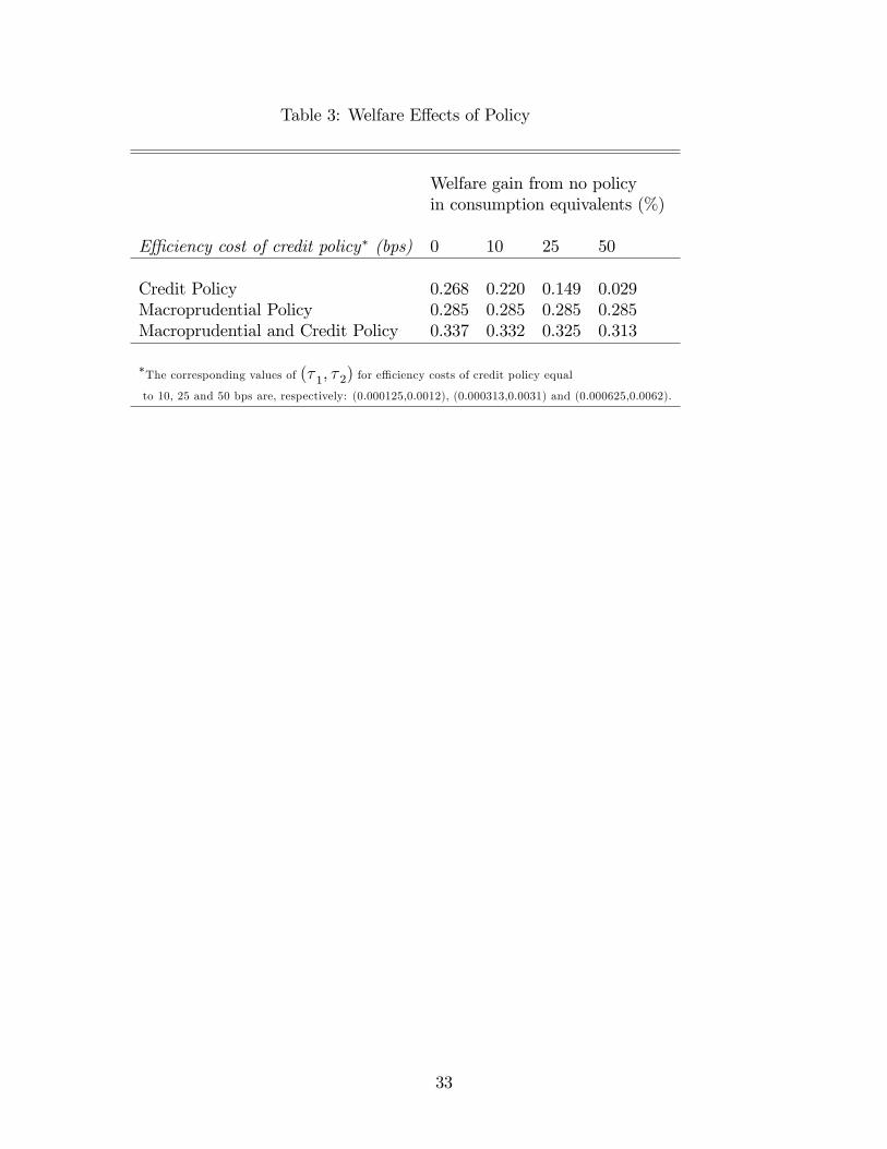
Table 3: Welfare E¤ects of Policy

Welfare gain from no policyin consumption equivalents (%)

E¢ ciency cost of credit policy� (bps) 0 10 25 50

Credit Policy 0.268 0.220 0.149 0.029Macroprudential Policy 0.285 0.285 0.285 0.285Macroprudential and Credit Policy 0.337 0.332 0.325 0.313

�The corresponding values of (� 1; � 2) for e¢ ciency costs of credit policy equalto 10, 25 and 50 bps are, respectively: (0.000125,0.0012), (0.000313,0.0031) and (0.000625,0.0062).

33

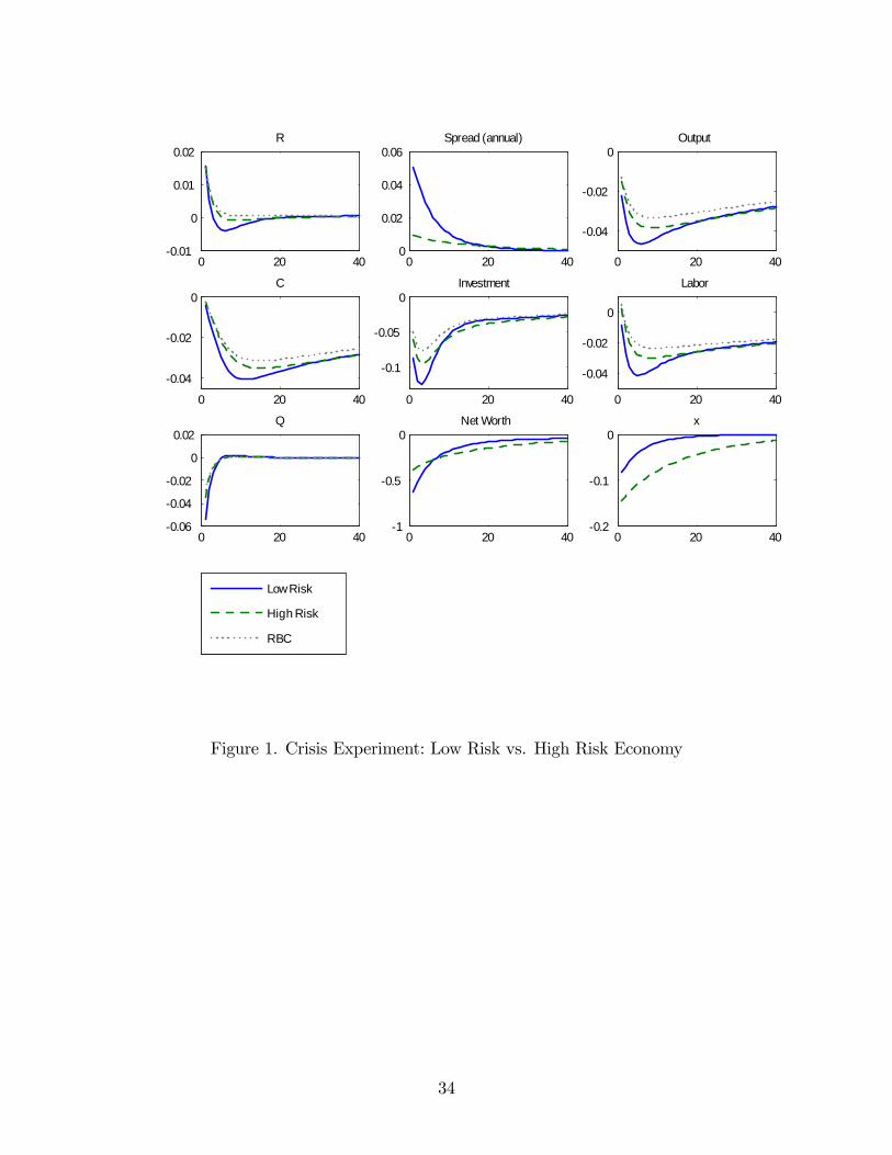
0 20 40­0.01

0

0.01

0.02R

0 20 400

0.02

0.04

0.06Spread (annual)

0 20 40

­0.04

­0.02

0Output

0 20 40

­0.04

­0.02

0C

0 20 40

­0.1

­0.05

0Investment

Low Risk

High Risk

RBC

0 20 40

­0.04

­0.02

0

Labor

0 20 40­0.06

­0.04

­0.02

0

0.02Q

0 20 40­1

­0.5

0Net Worth

0 20 40­0.2

­0.1

0x

Figure 1. Crisis Experiment: Low Risk vs. High Risk Economy

34

0 20 40­0.01

0

0.01

0.02R

0 20 400

0.02

0.04

0.06

0.08Spread (annual)

0 20 40­0.06

­0.04

­0.02

0Output

0 20 40­0.04

­0.02

0C

0 20 40

­0.1

­0.05

0Investment

Credit Policy ( νg = 100)

No Credit Policy

RBC

0 20 40

­0.04

­0.02

0

Labor

0 20 40­0.06

­0.04

­0.02

0

0.02Q

0 20 40­1

­0.5

0Net Worth

0 20 40­0.1

­0.05

0

x

0 20 400

0.1

0.2ζ

Figure 2. Credit Policy Response to Crisis: Low Risk Economy

35

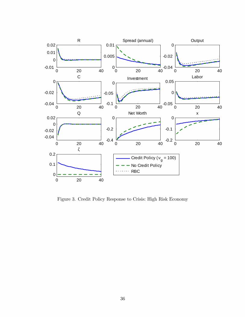
0 20 40­0.01

0

0.01

0.02R

0 20 400

0.005

0.01Spread (annual)

0 20 40­0.04

­0.02

0Output

0 20 40­0.04

­0.02

0C

0 20 40­0.1

­0.05

0Investment

Credit Policy (νg = 100)

No Credit PolicyRBC

0 20 40­0.05

0

0.05Labor

0 20 40­0.04­0.02

00.02

Q

0 20 40­0.4

­0.2

0Net Worth

0 20 40­0.2

­0.1

0x

0 20 400

0.1

0.2ζ

Figure 3. Credit Policy Response to Crisis: High Risk Economy

36

0 20 400

0.05

0.1

0.15

ζ

0 20 40­0.1

­0.05

0x

0 20 400

2

4

6x 10­3 Spread (annual)

0 20 40­0.04

­0.03

­0.02

­0.01Output

0 20 40­0.04

­0.02

0C

Anticipated Pol icy wi th νg=100

Unanticipated Pol icy with νg=50

RBC

0 20 40­0.1

­0.05

0Investment

Figure 4. Anticipated vs. Unanticipated Policy in High Risk Economy

37

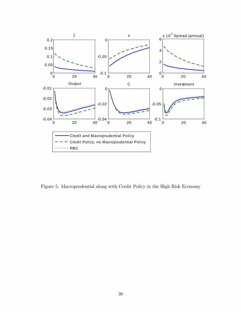
0 20 400

0.05

0.1

0.15

0.2ζ

0 20 40­0.1

­0.05

0x

0 20 400

2

4

6x 10­3 Spread (annual)

0 20 40­0.04

­0.03

­0.02

­0.01Output

0 20 40­0.04

­0.02

0C

0 20 40­0.1

­0.05

0Investment

Credi t and Macroprudential  PolicyCredi t Policy, no Macroprudential  Pol icyRBC

Figure 5. Macroprudential along with Credit Policy in the High Risk Economy

38

0 20 40­0.15

­0.1

­0.05

0

x

0 20 400

0.02

0.04

0.06Spread (annual)

0 20 40­0.05

­0.04

­0.03

­0.02

­0.01Output

0 20 40

­0.04

­0.03

­0.02

­0.01

0C

Macroprudential  PolicyNo Macroprudential  Pol icyRBC

0 20 40

­0.1

­0.05

0Investment

Figure 6. Macroprudential Policy without Credit Policy in the Low Risk Economy

39