Electronic copy available at: http://ssrn.com/abstract=1397239

1

Has the Basel II Accord Encouraged Risk Management

During the 2008-09 Financial Crisis?*

Michael McAleer

Econometric Institute Erasmus University Rotterdam

and Department of Applied Economics National Chung Hsing University

Taiwan

Juan-Angel Jimenez-Martin

Department of Quantitative Economics Complutense University of Madrid

Teodosio Pérez-Amaral

Department of Quantitative Economics Complutense University of Madrid

April 2009

* The first author wishes to thank the Australian Research Council for financial support. The second and third authors acknowledge the financial support of the Ministerio de Ciencia y Tecnología, Spain, and Comunidad de Madrid.

Electronic copy available at: http://ssrn.com/abstract=1397239

2

Abstract

The Basel II Accord requires that banks and other Authorized Deposit-taking

Institutions (ADIs) communicate their daily risk forecasts to the appropriate monetary

authorities at the beginning of each trading day, using one or more risk models to

measure Value-at-Risk (VaR). The risk estimates of these models are used to determine

capital requirements and associated capital costs of ADIs, depending in part on the

number of previous violations, whereby realised losses exceed the estimated VaR. In

this paper we define risk management in terms of choosing sensibly from a variety of

risk models, discuss the selection of optimal risk models, consider combining

alternative risk models, discuss the choice between a conservative and aggressive risk

management strategy, and evaluate the effects of the Basel II Accord on risk

management. We also examine how risk management strategies performed during the

2008-09 financial crisis, evaluate how the financial crisis affected risk management

practices, forecasting VaR and daily capital charges, and discuss alternative policy

recommendations, especially in light of the financial crisis. These issues are illustrated

using Standard and Poor’s 500 Index, with an emphasis on how risk management

practices were monitored and encouraged by the Basel II Accord regulations during the

financial crisis.

Key words and phrases: Value-at-Risk (VaR), daily capital charges, exogenous and endogenous violations, violation penalties, optimizing strategy, risk forecasts, aggressive or conservative risk management strategies, Basel II Accord, financial crisis.

JEL Classifications: G32, G11, G17, C53, C22.

3

1. Introduction

The financial crisis of 2008-09 has left an indelible mark on economic and financial

structures worldwide, and left an entire generation of investors wondering how things

could have become so severe. There have been many questions asked about whether

appropriate regulations were in place, especially in the USA, to permit the appropriate

monitoring and encouragement of (possibly excessive) risk taking.

The Basel II Accord was designed to monitor and encourage sensible risk taking using

appropriate models of risk to calculate Value-at-Risk (VaR) and subsequent daily

capital charges. VaR is defined as an estimate of the probability and size of the potential

loss to be expected over a given period, and is now a standard tool in risk management.

It has become especially important following the 1995 amendment to the Basel Accord,

whereby banks and other Authorized Deposit-taking Institutions (ADIs) were permitted

(and encouraged) to use internal models to forecast daily VaR (see Jorion (2000) for a

detailed discussion). The last decade has witnessed a growing academic and

professional literature comparing alternative modelling approaches to determine how to

measure VaR, especially for large portfolios of financial assets.

The amendment to the initial Basel Accord was designed to encourage and reward

institutions with superior risk management systems. A back-testing procedure, whereby

actual returns are compared with the corresponding VaR forecasts, was introduced to

assess the quality of the internal models used by ADIs. In cases where internal models

lead to a greater number of violations than could reasonably be expected, given the

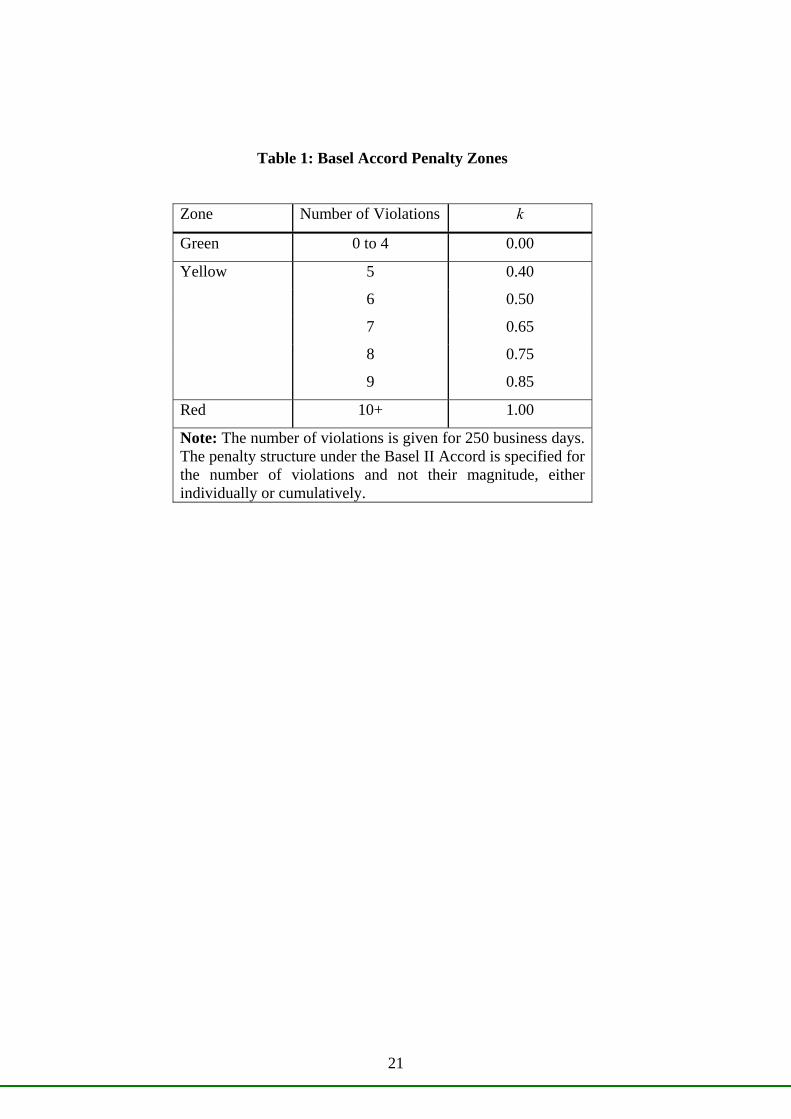
confidence level, the ADI is required to hold a higher level of capital (see Table 1 for

the penalties imposed under the Basel II Accord). Penalties imposed on ADIs affect

profitability directly through higher capital charges, and indirectly through the

imposition of a more stringent external model to forecast VaR. This is one reason why

financial managers may prefer risk management strategies that are passive and

conservative rather than active and aggressive.

Excessive conservatism can have a negative impact on the profitability of ADIs as

higher capital charges are subsequently required. Therefore, ADIs should perhaps

consider a strategy that allows an endogenous decision as to how many times ADIs

4

should violate in any financial year (for further details, see McAleer and da Veiga

(2008a, 2008b), McAleer (2008), Caporin and McAleer (2009b) and McAleer et al.

(2009)). This paper suggests alternative aggressive and conservative risk management

strategies that can be compared with the use of one or more models of risk throughout

the estimation and forecasting periods.

This paper defines risk management in terms of choosing sensibly from a variety of risk

models, discusses the selection of optimal risk models, considers combining alternative

risk models, discusses the choice between conservative and aggressive risk management

strategies, evaluates the effects of the Basel II Accord on risk management, examines

how risk management strategies performed during the 2008-09 financial crisis,

evaluates how the financial crisis affected risk management practices, forecasts VaR

and daily capital charges, and discusses alternative policy recommendations, especially

in light of the financial crisis.

These issues are illustrated using Standard and Poor’s 500 Index, with an emphasis on

how risk management practices were monitored and encouraged by the Basel II Accord

regulations during the financial crisis.

The remainder of the paper is as follows. In Section 2 we present the main ideas of the

Basel II Accord Amendment as it relates to forecasting VaR and daily capital charges.

Section 3 reviews some of the most well known models of volatility that are used to

forecast VaR and calculate daily capital charges, and presents aggressive and

conservative bounds on risk management strategies. In Section 4 the data used for

estimation and forecasting are presented. Section 5 analyses the forecast values of VaR

and daily capital charges before and during the 2008-08 financial crisis, and Section 6

summarizes the main conclusions.

2. Forecasting Value-at-Risk and Daily Capital Charges

The Basel II Accord stipulates that daily capital charges (DCC) must be set at the higher

of the previous day’s VaR or the average VaR over the last 60 business days, multiplied

by a factor (3+k) for a violation penalty, wherein a violation involves the actual negative

returns exceeding the VaR forecast negative returns for a given day:

5

( ){ }______

60 1sup 3 VaR , VaRt tDCC k −= − + − (1)

where

DCC = daily capital charges, which is the higher of ( ) 160

______VaR and VaR3 −−+− tk ,

tVAR = Value-at-Risk for day t,

tttt zYVAR σˆ ⋅−= ,

60

______

VaR = mean VaR over the previous 60 working days,

tY = estimated return at time t,

tz = 1% critical value of the distribution of returns at time t,

tσ = estimated risk (or square root of volatility) at time t,

10 ≤≤ k is the Basel II violation penalty (see Table 1).

[Table 1 goes here]

The multiplication factor (or penalty), k, depends on the central authority’s assessment

of the ADI’s risk management practices and the results of a simple back test. It is

determined by the number of times actual losses exceed a particular day’s VaR forecast

(Basel Committee on Banking Supervision (1996)). The minimum multiplication factor

of 3 is intended to compensate for various errors that can arise in model

implementation, such as simplifying assumptions, analytical approximations, small

sample biases and numerical errors that tend to reduce the true risk coverage of the

model (see Stahl (1997)). Increases in the multiplication factor are designed to increase

the confidence level that is implied by the observed number of violations to the 99 per

cent confidence level, as required by the regulators (for a detailed discussion of VaR, as

well as exogenous and endogenous violations, see McAleer (2008), Jiménez-Martin et

al. (2009), and McAleer et al. (2009)).

6

In calculating the number of violations, ADIs are required to compare the forecasts of

VaR with realised profit and loss figures for the previous 250 trading days. In 1995, the

1988 Basel Accord (Basel Committee on Banking Supervision (1988) was amended to

allow ADIs to use internal models to determine their VaR thresholds (Basel Committee

on Banking Supervision (1995)). However, ADIs that proposed using internal models

are required to demonstrate that their models are sound. Movement from the green zone

to the red zone arises through an excessive number of violations. Although this will lead

to a higher value of k, and hence a higher penalty, a violation will also tend to be

associated with lower daily capital charges.

Value-at-Risk refers to the lower bound of a confidence interval for a (conditional)

mean, that is, a “worst case scenario on a typical day”. If interest lies in modelling the

random variable, Yt , it could be decomposed as follows:

1( | )t t t tY E Y F ε−= + . (2)

This decomposition states that Yt comprises a predictable component, E(Yt | Ft−1) ,

which is the conditional mean, and a random component, εt . The variability of Yt , and

hence its distribution, is determined by the variability of εt . If it is assumed that εt

follows a distribution such that:

),(~ 2

ttt D σμε (3)

where μt and σ t are the unconditional mean and standard deviation of εt , respectively,

these can be estimated using a variety of parametric, semi-parametric or non-parametric

methods. The VaR threshold for Yt can be calculated as:

1( | )t t t tVaR E Y F ασ−= − , (3)

where α is the critical value from the distribution of εt to obtain the appropriate

confidence level. It is possible for σ t to be replaced by alternative estimates of the

conditional variance in order to obtain an appropriate VaR (for useful reviews of

7

theoretical results for conditional volatility models, see Li et al. (2002) and McAleer

(2005),who discusses a variety of univariate and multivariate, conditional, stochastic

and realized. volatility models).

Some recent empirical studies (see, for example, Berkowitz and O'Brien (2001) and

Gizycki and Hereford (1998)) have indicated that some financial institutions

overestimate their market risks in disclosures to the appropriate regulatory authorities,

which can imply a costly restriction to the banks trading activity. ADIs may prefer to

report high VaR numbers to avoid the possibility of regulatory intrusion. This

conservative risk reporting suggests that efficiency gains may be feasible. In particular,

as ADIs have effective tools for the measurement of market risk, while satisfying the

qualitative requirements, ADIs could conceivably reduce daily capital charges by

implementing a context-dependent market risk disclosure policy. For a discussion of

alternative approaches to optimize VaR and daily capital charges, see McAleer (2008)

and McAleer et al. (2009).

The next section describes several volatility models that are widely used to forecast the

1-day ahead conditional variances and VaR thresholds.

3. Models for Forecasting VaR

As discussed previously, ADIs can use internal models to determine their VaR

thresholds. There are alternative time series models for estimating conditional volatility.

In what follows, we present several conditional volatility models to evaluate strategic

market risk disclosure, namely GARCH, GJR and EGARCH, with both normal and t

distribution errors, where the degrees of freedom are estimated. For an extensive

discussion of the theoretical properties of several of these models, see Ling and

McAleer (2002a, 2002b, 2003a) and Caporin and McAleer (2009b). As an alternative to

estimating the parameters, we also consider the exponential weighted moving average

(EWMA) method by RiskmetricsTM (1996) that calibrates the unknown parameters.

Apart from EWMA, the models are presented in increasing order of complexity.

8

3.1 GARCH

For a wide range of financial data series, time-varying conditional variances can be

explained empirically through the autoregressive conditional heteroskedasticity

(ARCH) model, which was proposed by Engle (1982). When the time-varying

conditional variance has both autoregressive and moving average components, this

leads to the generalized ARCH(p,q), or GARCH(p,q), model of Bollerslev (1986). It is

very common to impose the widely estimated GARCH(1,1) specification in advance.

Consider the stationary AR(1)-GARCH(1,1) model for daily returns, ty :

t 1 2 t-1 t 2y = φ +φ y +ε , φ < 1 (4)

for nt ,...,1= , where the shocks to returns are given by:

t t t t

2t t -1 t-1

ε = η h , η ~ iid(0,1)

h =ω+αε + βh , (5)

and 0, 0, 0ω α β> ≥ ≥ are sufficient conditions to ensure that the conditional variance

0>th . The stationary AR(1)-GARCH(1,1) model can be modified to incorporate a non-

stationary ARMA(p,q) conditional mean and a stationary GARCH(r,s) conditional

variance, as in Ling and McAleer (2003b).

3.2 GJR

In the symmetric GARCH model, the effects of positive shocks (or upward movements

in daily returns) on the conditional variance, th , are assumed to be the same as the

negative shocks (or downward movements in daily returns). In order to accommodate

asymmetric behaviour, Glosten, Jagannathan and Runkle (1992) proposed a model

(hereafter GJR), for which GJR(1,1) is defined as follows:

2t t-1 t -1 t-1h =ω+(α+ γI(η ))ε + βh , (6)

9

where 0,0,0,0 ≥≥+≥> βγααω are sufficient conditions for ,0>th and )( tI η is an

indicator variable defined by:

( )1, 00, 0

tt

t

Iε

ηε<⎧

= ⎨ ≥⎩ (7)

as tη has the same sign as tε . The indicator variable differentiates between positive

and negative shocks, so that asymmetric effects in the data are captured by the

coefficient γ . For financial data, it is expected that 0≥γ because negative shocks

have a greater impact on risk than do positive shocks of similar magnitude. The

asymmetric effect, ,γ measures the contribution of shocks to both short run persistence,

2α γ+ , and to long run persistence, 2α β γ+ + . Although GJR permits asymmetric

effects of positive and negative shocks of equal magnitude on conditional volatility, the

special case of leverage, whereby negative shocks increase volatility while positive

shocks decrease volatility (see Black (1976) for an argument using the debt/equity

ratio), cannot be accommodated.

3.3 EGARCH

An alternative model to capture asymmetric behaviour in the conditional variance is the

Exponential GARCH, or EGARCH(1,1), model of Nelson (1991), namely:

t -1 t-1t t-1

t-1 t-1

ε εlogh =ω+α + γ + βlogh , | β |< 1h h

(8)

where the parameters α , β and γ have different interpretations from those in the

GARCH(1,1) and GJR(1, 1) models.

EGARCH captures asymmetries differently from GJR. The parameters α and γ in

EGARCH(1,1) represent the magnitude (or size) and sign effects of the standardized

residuals, respectively, on the conditional variance, whereas α and γα + represent the

effects of positive and negative shocks, respectively, on the conditional variance in

10

GJR(1,1). Unlike GJR, EGARCH can accommodate leverage, depending on restrictions

imposed on the size and sign parameters.

As noted in McAleer et al. (2007), there are some important differences between

EGARCH and the previous two models, as follows: (i) EGARCH is a model of the

logarithm of the conditional variance, which implies that no restrictions on the

parameters are required to ensure 0>th ; (ii) moment conditions are required for the

GARCH and GJR models as they are dependent on lagged unconditional shocks,

whereas EGARCH does not require moment conditions to be established as it depends

on lagged conditional shocks (or standardized residuals); (iii) Shephard (1996) observed

that 1|| <β is likely to be a sufficient condition for consistency of QMLE for

EGARCH(1,1); (iv) as the standardized residuals appear in equation (7), 1|| <β would

seem to be a sufficient condition for the existence of moments; and (v) in addition to

being a sufficient condition for consistency, 1|| <β is also likely to be sufficient for

asymptotic normality of the QMLE of EGARCH(1,1).

3.4 Exponentially Weighted Moving Average (EWMA)

The three conditional volatility models given above are estimated under the following

distributional assumptions on the conditional shocks: (1) normal, and (2) t, with

estimated degrees of freedom. As an alternative to estimating the parameters of the

appropriate conditional volatility models, RiskmetricsTM (1996) developed a model

which estimates the conditional variances and covariances based on the exponentially

weighted moving average (EWMA) method, which is, in effect, a restricted version of

the ARCH(∞ ) model. This approach forecasts the conditional variance at time t as a

linear combination of the lagged conditional variance and the squared unconditional

shock at time 1t − . The EWMA model calibrates the conditional variance as:

2t t-1 t-1h = λh +(1- λ)ε (9)

where λ is a decay parameter. Riskmetrics™ (1996) suggests that λ should be set at

0.94 for purposes of analysing daily data. As no parameters are estimated, there is no

11

need to establish any moment or log-moment conditions for purposes of demonstrating

the statistical properties of the estimators.

4. Data

The data used for estimation and forecasting are the closing daily prices for Standard

and Poor’s Composite 500 Index (S&P500), which were obtained from the Ecowin

Financial Database for the period 3 January 2000 to 12 February 2009.

If tP denotes the market price, the returns at time t ( )tR are defined as:

( )1log / −=t t tR P P . (10)

[Insert Figure 1 here]

Figure 1 shows the S&P500 returns, for which the descriptive statistics are given in

Table 2. The extremely high positive and negative returns are evident from September

2008 onward, and have continued well into 2009. The mean is close to zero, and the

range is between -11% and -9.5%. The Jarque-Bera Lagrange multiplier test for

normality rejects the null hypothesis of normally distributed returns. As the series

displays high kurtosis, this would seem to indicate the existence of extreme

observations, as can be seen in the histogram, which is not surprising for financial

returns data.

[Insert Table 2 here]

Several measures of volatility are available in the literature. In order to gain some

intuition, we adopt the measure proposed in Franses and van Dijk (1999), where the true

volatility of returns is defined as:

( )( )21| −= −t t t tV R E R F , (11)

where 1−tF is the information set at time t-1.

12

Figure 2 shows the S&P500 volatility, as defined in equation (11). The series exhibit

clustering that needs to be captured by an appropriate time series model. The volatility

of the series appears to be high during the early 2000s, followed by a quiet period from

2003 to the beginning of 2007. Volatility increases dramatically after August 2008, due

in large part to the worsening global credit environment. This increase in volatility is

even higher in October 2008. In less than 4 weeks in October 2008, the S&P500 index

plummeted by 27.1%. In less than 3 weeks in November 2008, starting the morning

after the US elections, the S&P500 index plunged a further 25.2%. Overall, from late

August 2008, US stocks fell by an almost unbelievable 42.2% to reach a low on 20

November 2008.

An examination of daily movements in the S&P500 index back to 2000 suggests that

large changes by historical standards are 4% in either direction. From January 2000 to

March 2008, there was a 0.4% chance of observing an increase of 4% or more in one

day, and a 0.2% chance of seeing a reduction of 4% or more in one day. Therefore,

99.4% of movements in the S&P500 index during this period had daily swings of less

than 4%. Prior to September 2008, the S&P500 index had only 24 days with massive

4% gains, but since September 2008, there have been 12 more such days. On the

downside, before the current stock market meltdown, the S&P500 index had only 18

days with huge 4% or more losses, whereas during the recent panic, there were a further

15 such days.

This comparison is between more than 58 years and just six months. During this short

time span of financial panic, the 4% or more gain days increased by 72%, while the

number of 4% or more loss days increased by 106%. Such movements in the S&P500

index are unprecedented.

Alternative models of volatility can be compared on the basis of statistical significance,

goodness of fit, forecasting VaR, calculation of daily capital charges, and optimality on

a daily or temporally aggregated basis. As the focus of forecasting VaR is to calculate

daily capital charges, subject to appropriate penalties, the most severe of which is

temporary or permanent suspension from investment activities, the goodness of fit

criterion used is the calculation of daily and mean capital charges, both before and after

the 2008-09 financial crisis.

13

5. Forecasting VaR and Calculating Daily Capital Charges

In this section, the forecast values of VaR and daily capital charges are analysed before

and during the 2008-09 financial crisis. We consider alternative risk management

strategies and propose some policy recommendations.

In Figure 3, VaR forecasts are compared with S&P500 returns, where the vertical axis

represents returns, and the horizontal axis represents the days from 2 January 2008 to 12

February 2009. The S&P500 returns are given as the upper blue line that fluctuates

around zero.

ADIs need not restrict themselves to using only one of the available risk models. In this

paper we propose a risk management strategy that consists in choosing from among

different combinations of alternative risk models to forecast VaR. We first discuss a

combination of models that can be characterized as an aggressive strategy and another

that can be regarded as a conservative strategy, as given in Figure 3.

The upper red line represents the infinum of the VaR calculated for the individual

models of volatility, which reflects an aggressive risk management strategy, whereas the

lower green line represents the supremum of the VaR calculated for the individual

models of volatility, which reflects a conservative risk management strategy. These two

lines correspond to a combination of alternative risk models.

[Insert Figure 3 here]

As can be seen in Figure 3, VaR forecasts obtained from the different models of

volatility have fluctuated, as expected, during the first few months of 2008. It has been

relatively low, at below 5%, and relatively stable between April and August 2008.

Around September 2008, VaR started increasing until it peaked in October 2008,

between 10% and 15%, depending on the model of volatility considered. This is

essentially a four-fold increase in VaR in a matter of one and a half months. In the last

two months of 2008, VaR decreased to values between 5% and 8%, which is still twice

as large as it had been just a few months earlier. Therefore, volatility has increased

substantially during the financial crisis, and has remained relatively high after the crisis.

14

Figure 4 includes daily capital charges based on VaR forecasts and the mean VAR for

the previous 60 days, which are the two lower smooth lines. The red line corresponds to

the aggressive risk management strategy based on the infinum of the daily capital

charges of the alternative models of volatility, and the green line corresponds to the

conservative risk management strategy based on the supremum of the daily capital

charges of the alternative models of volatility.

Before the financial crisis, there is a substantial difference between the two lines

corresponding to the aggressive and conservative risk management strategies. However

at the onset of the crisis, the two lines virtually coincide, which suggests that the

moving average term in the Basel II formula, which dominates the calculation of daily

capital charges, is excessive. This suggests that the use of a shorter moving average in

the Basel II formula for calculating the DCC may lead to a closer vertical alignment

between the troughs of the VaR and DCC lines, thereby leading to a closer

correspondence between high values of VaR and high values of DCC, as may be

desirable.

After the crisis had begun, there is a substantial difference between the two strategies,

arising from divergence across the alternative models of volatility, and hence between

the aggressive and conservative risk management strategies.

[Insert Figure 4 here]

It can be observed from Figure 4 that daily capital charges always exceed VaR (in

absolute terms). Moreover, immediately after the financial crisis had started, a

significant amount of capital was set aside to cover likely financial losses. This is a

positive feature of the Basel II Accord, since it can have the effect of shielding ADIs

from possible significant financial losses.

The Basel II Accord would seem to have succeeded in covering the losses of ADIs

before, during and after the financial crisis. Therefore, it is likely to be useful when

extended to countries to which it does not currently apply.

15

[Insert Figure 5 here]

Figure 5 shows the accumulated number of violations for each model of volatility over

the period of 260 days considered (2 January 2008 to 12 February 2009). Table 3 gives

the percentage of days for which daily capital charges are minimized, the mean daily

capital charges, and the number of violations for the alternative models of volatility.

The upper red line in Figure 5 corresponds to the aggressive risk management strategy,

which yields 16 violations, thereby exceeding the recommended limit of 10 in 250

working days. The lower green line corresponds to the conservative risk management

strategy, which gives only 3 violations. Although this small number of violations is well

within the Basel II limits, it may, in fact, be too few as it is likely to lead to considerably

higher daily capital charges.

It may be useful to consider other strategies that lie somewhat in the middle of the

previous two, such as the median or the average value of the VaR forecasts for a given

day. Another possibility could be the DYLES strategy, developed in McAleer et al.

(2009), which seems to work well in practice.

It is also worth noting from Table 3 and Figure 6, which gives the duration of the

minimum daily capital charges for the alternative models of volatility, that four models

of risk, including the conservative risk management strategy, do not minimize daily

capital charges for even one day. On the other hand, the aggressive risk management

strategy minimizes the mean daily capital charge over the year relative to its

competitors, and also has the highest frequency of minimizing daily capital charges.

The EGARCH model with t distribution errors also minimizes daily capital charges

frequently, and has a low mean daily capital charge. However, it is interesting that the

EGARCH model with normal errors has a mean daily capital charge that is almost as

low as that of the aggressive risk management strategy, even though it rarely minimizes

daily capital charges.

[Insert Figure 6 here]

In terms of choosing the appropriate risk model for minimizing DCC, the simulations

results reported here would suggest the following:

16

(1) Before the financial crisis, the best models for minimizing daily capital charges are

GARCH and GJR.

(2) During the financial crisis, the best model is Riskmetrics.

(3) After the financial crisis, the best model is TEGARCH.

The financial crisis has affected risk management strategies by changing the optimal

model for minimizing daily capital charges.

6. Conclusion

Under the Basel II Accord, ADIs have to communicate their risk estimates to the

monetary authorities, and use a variety of VaR models to estimate risks. ADIs are

subject to a back-test that compares the daily VaR to the subsequent realized returns,

and ADIs that fail the back-test can be subject to the imposition of standard models that

can lead to higher daily capital costs. Additionally, the Basel II Accord stipulates that

the daily capital charge that the bank must carry as protection against market risk must

be set at the higher of the previous day’s VaR or the average VaR over the last 60

business days, multiplied by a factor 3+k. An ADI’s objective is to maximize profits, so

they wish to minimize their capital charges while restricting the number of violations in

a given year below the maximum of 10 allowed by the Basel II Accord.

In this paper we defined risk management in terms of choosing sensibly from a variety

of conditional volatility (or risk) models, discussed the selection of optimal risk models,

considered combining alternative risk models, choosing between a conservative and

aggressive risk management strategy and evaluating the effects of the Basel II Accord

on risk management. We also examined how risk management strategies performed

during the 2008-09 financial crisis, evaluated how the financial crisis affected risk

management practices, forecasted VaR and daily capital charges, and discussed

alternative policy recommendations, especially in light of the 2008-09 financial crisis.

These issues were illustrated using Standard and Poor’s 500 Index, with an emphasis on

how risk management practices were monitored and encouraged by the Basel II Accord

regulations during the financial crisis.

17

Volatility has increased four-fold during the 2008-09 financial crisis, and remained

relatively high after the crisis. This may be a reason why the financial crisis has changed

the choice of risk management model for optimizing daily capital charges. Alternative

risk models were found to be optimal before and during the financial crisis.

In this paper we proposed the idea of constructing risk management strategies that used

combinations of several models for forecasting VaR. It was found that an aggressive

risk management strategy yielded the lowest mean capital charges, and had the highest

frequency of minimizing daily capital charges throughout the forecasting period, but

which also tended to violate too often. Such excessive violations can have the effect of

leading to unwanted publicity, and temporary or permanent suspension from trading as

an ADI. On the other hand, a conservative risk management strategy would have far

fewer violations, and a correspondingly higher mean daily capital charge.

The area between the bounds provided by the aggressive and conservative risk

management strategies would seem to be a fertile area for future research.

A risk management strategy that used different combinations of alternative risk models

for predicting VaR and minimizing daily capital charges was found to be optimal. A

risk model that leads to the median forecast of VaR may also be a useful risk

management strategy, as would be the DYLES strategy established in McAleer et al.

(2009).

The Basel II Accord rules have been successful in covering the losses of ADIs before,

during and after the 2008-09 financial crisis. Their application could be recommended

for as yet unregulated markets and countries. Another recommendation would be to

modify the Basel II Accord for calculating daily capital charges to shorten the moving

average, to (say) 20 days, from the current 60 previous working days. This would allow

a speedier adjustment of daily capital charges to changes in VaR, thereby avoiding the

excessive lags observed in the simulations reported in the paper.

18

References

Basel Committee on Banking Supervision, (1988), International Convergence of Capital

Measurement and Capital Standards, BIS, Basel, Switzerland.

Basel Committee on Banking Supervision, (1995), An Internal Model-Based Approach

to Market Risk Capital Requirements, BIS, Basel, Switzerland.

Basel Committee on Banking Supervision, (1996), Supervisory Framework for the Use

of “Backtesting” in Conjunction with the Internal Model-Based Approach to

Market Risk Capital Requirements, BIS, Basel, Switzerland.

Berkowitz, J. and J. O'Brien (2001), How accurate are value-at-risk models at

commercial banks?, Discussion Paper, Federal Reserve Board.

Black, F. (1976), Studies of stock market volatility changes, in 1976 Proceedings of the

American Statistical Association, Business and Economic Statistics Section, pp.

177-181.

Bollerslev, T. (1986), Generalised autoregressive conditional heteroscedasticity, Journal

of Econometrics, 31, 307-327.

Caporin, M. and M. McAleer (2009a), Do we really need both BEKK and DCC? A tale

of two covariance models (Available at SSRN: http://ssrn.com/abstract=1338190).

Caporin, M. and M. McAleer (2009b), The Ten Commandments for managing

investments, to appear in Journal of Economic Surveys (Available at SSRN:

http://ssrn.com/abstract=1342265).

Engle, R.F. (1982), Autoregressive conditional heteroscedasticity with estimates of the

variance of United Kingdom inflation, Econometrica, 50, 987-1007.

Franses, P.H. and D. van Dijk (1999), Nonlinear Time Series Models in Empirical

Finance, Cambridge, Cambridge University Press.

Gizycki, M. and N. Hereford (1998), Assessing the dispersion in banks’ estimates of

market risk: the results of a value-at-risk survey, Discussion Paper 1, Australian

Prudential Regulation Authority.

Glosten, L., R. Jagannathan and D. Runkle (1992), On the relation between the expected

value and volatility of nominal excess return on stocks, Journal of Finance, 46,

1779-1801.

Jimenez-Martin, J.-A., McAleer, M. and T. Peréz-Amaral (2009), The Ten

Commandments for managing value-at-risk under the Basel II Accord, to appear

19

in Journal of Economic Surveys (Available at SSRN:

http://ssrn.com/abstract=1356803).

Jorion, P. (2000), Value at Risk: The New Benchmark for Managing Financial Risk,

McGraw-Hill, New York.

Li, W.K., S. Ling and M. McAleer (2002), Recent theoretical results for time series

models with GARCH errors, Journal of Economic Surveys, 16, 245-269.

Reprinted in M. McAleer and L. Oxley (eds.), Contributions to Financial

Econometrics: Theoretical and Practical Issues, Blackwell, Oxford, 2002, pp. 9-

33.

Ling, S. and M. McAleer (2002a), Stationarity and the existence of moments of a family

of GARCH processes, Journal of Econometrics, 106, 109-117.

Ling, S. and M. McAleer (2002b), Necessary and sufficient moment conditions for the

GARCH(r,s) and asymmetric power GARCH(r, s) models, Econometric Theory,

18, 722-729.

Ling, S. and M. McAleer, (2003a), Asymptotic theory for a vector ARMA-GARCH

model, Econometric Theory, 19, 278-308.

Ling, S. and M. McAleer (2003b), On adaptive estimation in nonstationary ARMA

models with GARCH errors, Annals of Statistics, 31, 642-674.

McAleer, M. (2005), Automated inference and learning in modeling financial volatility,

Econometric Theory, 21, 232-261.

McAleer, M. (2008), The Ten Commandments for optimizing value-at-risk and daily

capital charges, to appear in Journal of Economic Surveys (Available at SSRN:

http://ssrn.com/abstract=1354686).

McAleer, M., F. Chan and D. Marinova (2007), An econometric analysis of asymmetric

volatility: theory and application to patents, Journal of Econometrics, 139, 259-

284.

McAleer, M., J.-Á. Jiménez-Martin and T. Peréz-Amaral (2009), A decision rule to

minimize daily capital charges in forecasting value-at-risk (Available at SSRN:

http://ssrn.com/abstract=1349844).

McAleer, M. and B. da Veiga (2008a), Forecasting value-at-risk with a parsimonious

portfolio spillover GARCH (PS-GARCH) model, Journal of Forecasting, 27, 1-19.

McAleer, M. and B. da Veiga (2008b), Single index and portfolio models for

forecasting value-at-risk thresholds, Journal of Forecasting, 27, 217-235.

20

Nelson, D.B. (1991), Conditional heteroscedasticity in asset returns: a new approach,

Econometrica, 59, 347-370.

RiskmetricsTM (1996), J.P. Morgan Technical Document, 4th Edition, New York, J.P.

Morgan.

Shephard, N. (1996), Statistical aspects of ARCH and stochastic volatility, in O.E.

Barndorff-Nielsen, D.R. Cox and D.V. Hinkley (eds.), Statistical Models in

Econometrics, Finance and Other Fields, Chapman & Hall, London, pp. 1-67.

Stahl, G. (1997), Three cheers, Risk, 10, 67-69.

21

Table 1: Basel Accord Penalty Zones

Zone Number of Violations k

Green 0 to 4 0.00

Yellow 5 0.40

6 0.50

7 0.65

8 0.75

9 0.85

Red 10+ 1.00

Note: The number of violations is given for 250 business days. The penalty structure under the Basel II Accord is specified for the number of violations and not their magnitude, either individually or cumulatively.

22

Table 2. Descriptive Statistics for S&P500 Returns

3 January 2000 – 12 February 2009

0

200

400

600

800

1,000

-10 -8 -6 -4 -2 0 2 4 6 8 10

Series: S&P 500 returns (%)Sample 3/01/2000 12/02/2009Observations 2378

Mean -0.023350Median 0.000177Maximum 10.95792Minimum -9.469733Std. Dev. 1.352380Skewness -0.158294Kurtosis 11.92801

Jarque-Bera 7907.807Probability 0.000000

23

Table 3. Percentage of Days Minimizing Daily Capital Charges, Mean Daily Capital Charges, and Number of Violations for Alternative Models of Volatility

Model % of Days

Minimizing Daily Capital Charges

Mean Daily Capital Charges

Number of Violations

Riskmetrics 14.0 % 0.163 10 GARCH 0.0 % 0.161 13 GJR 10.0 % 0.157 7 EGARCH 1.70 % 0.146 13 GARCH_t 0.00 % 0.171 3 GJR_t 0.00 % 0.167 3 EGARCH_t 34.0 % 0.153 3 Lower bound 0.00 % 0.177 3 Upper bound 39.6 % 0.143 16

24

Figure 1. Daily Returns on the S&P500 Index,

3 January 2000 – 12 February 2009

-12%

-8%

-4%

0%

4%

8%

12%

3/1/00 1/1/02 1/1/04 2/1/06 1/1/08

25

Figure 2. Daily Volatility in S&P500 Returns

3 January 2000 – 12 February 2009

0.0%

0.2%

0.4%

0.6%

0.8%

1.0%

1.2%

3/1/00 1/1/02 1/1/04 2/1/06 1/1/08

26

Figure 3. VaR for S&P500 Returns

2 January 2008 – 12 February 2009

-20%

-15%

-10%

-5%

0%

5%

10%

15%

1/1/08 1/4/08 1/7/08 1/10/08 1/1/09

S&P Returns VaR EGARCHVaR GARCH VaR GARCH_tVaR GJR VaR GJR_tVaR lowerbound VaR RSKMVaR upperbound VaR EGARCH_t

Note: The upper blue line represents daily returns for the S&P500 index. The upper red line represents the infinum of the VaR forecasts for the different models described in Section 3. The lower green line corresponds to the supremum of the forecasts of the VaR for the same models.

27

Figure 4. VaR and Mean VaR for the Previous 60 Days to Calculate

Daily Capital Charges for S&P Returns

-.5

-.4

-.3

-.2

-.1

.0

.1

.2

2008Q1 2008Q2 2008Q3 2008Q4

S&P_returnsVARF_EGARCHVARF_GARCHVARF_GARCH_TVARF_GJRVARF_GJR_TVARF_lowerboundVARF_RSKMVARF_upperboundVARF_TEGARCH-mean(var_last60days)_EGARCH-mean(var_last60days)_GARCH-mean(var_last60days)_GARCH_T-mean(var_last60days)_GJR-mean(var_last60days)_GJR_T-mean(var_last60days)_lowerbound-mean(var_last60days)_RSKM-mean(var_last60days)_upperbound-mean(var_last60days)_TEGARCH

28

Figure 5. Number of Violations Accumulated Over 260 Days

0

4

8

12

16

20

2008Q1 2008Q2 2008Q3 2008Q4

NOV_ACCU_RSKMNOV_ACCU_GARCHNOV_ACCU_GJRNOV_ACCU_EGARCHNOV_ACCU_GARCH_TNOV_ACCU_GJR_TNOV_ACCU_TEGARCHNOV_ACCU_lowerboundNOV_ACCU_upperbound

29

Figure 6. Duration of Minimum Daily Capital Charges for

Alternative Models of Volatility

0

1

2

2008Q1 2008Q2 2008Q3 2008Q4

MIN_EGARCH MIN_GARCHMIN_GARCH_T MIN_GJRMIN_GJR_T MIN_lowerboundMIN_RSKM MIN_upperboundMIN_TEGARCH