Financial Data Analysis

Multivariate GARCH

July 13, 2010

Multivariate GARCH Models

• C. Alexander (2008): Practical Financial Econometrics, Chapter II.4.5.

• A. Silvennoinen and T. Terasvirta (2009): Multivariate GARCHModels, Handbook of Financial Time Series, Springer; available athttp://papers.ssrn.com/sol3/papers.cfm?abstract id=1148139.

• L. Bauwens and S. Laurent and J. K. Rombouts (2006): MultivariateGARCH Models: A Survey, Journal of Applied Econometrics, 21, 79–109;available at http://ideas.repec.org/p/cor/louvco/2003031.html.

1

Multivariate GARCH

• Many problems in finance are inherently multivariate and require us tounderstand the dependence structure between assets.

• E.g.,

– portfolio analysis,– volatility transmission: study of relations between the volatilities

and covariances/correlations of several markets (e.g., emerging anddeveloped markets, or different regions),

– relation between correlations and volatilities,– tests of asset pricing models,– futures hedging.

• Multivariate GARCH: Models for the evolution of volatilities andcovariances/correlations.

2

• Consider a return vector rt consisting of N components, i.e., rt =[r1t, r2t, . . . , rNt]′ (a column vector),

rt = µt + εt (1)

µt = E(rt|It−1) = Et−1(rt) (2)

εt|It−1 ∼ N(0,Ht) (3)

Ht = Var(rt|It−1) = Vart−1(rt) = Vart−1(εt), (4)

where It is the information available at time t, usually It = {rt, rt−1, . . .}.

• The error termεt = [ε1t, ε2t, . . . , εNt]′.

• This implies that Ht is the conditional covariance matrix of rt.

3

• Covariance matrix

Ht =

h21t h12,t h13,t · · · h1N,t

h12,t h22t h23,t · · · h2N,t

h213,t h23,t h2

3,t · · · h3N,t... ... ... . . . ...

h1N,t h2N,t h3N,t · · · h2Nt

, (5)

whereh2

jt = Vart−1(rjt), hij,t = Covt−1(rit, rjt), (6)

is symmetric and positive definite:

• We know that for any linear combination (with weight vector w =[w1, w2, . . . , wN ]′) of the elements of rt,

1

0 < Vart−1

(∑

i

wirit

)=

∑

i

w2i h

2i,t +

∑

i

∑

j 6=i

wiwjhij,t = w′Htw.

1The variance may be zero if the components are linearly dependent.

4

• For example, with N = 2,

Vart−1(w1r1t + w2r2t) = w21h

21t + 2w1w2h12,t + w2

2h22t

=[

w1 w2

] [h2

1t h12,t

h12,t h22t

] [w1

w2

].

• If the conditional distribution of rt is multivariate normal, then, forexample, the conditional 100×ξ% portfolio Value–at–Risk (VaR) for anyportfolio combination w can be calculated as

VaRt−1(ξ) = w′µt + Φ−1(ξ)√

w′Htw, (7)

where Φ−1(ξ) is the ξ–quantile of the standard normal distribution, e.g.,Φ−1(0.01) = −2.3263 and Φ−1(0.05) = −1.6449.

5

• Similar to the univariate GARCH,

rt = µt + εt, εt = σtηt, ηtiid∼ N(0, 1),

(3) is often written as

εt = H1/2t zt, zt

iid∼ N(0, I), (8)

where N(0, I) denotes the N–dimensional normal distribution with amean vector of zeros and identity covariance matrix, i.e., the N -dimensional standard normal.

• H1/2t is an N ×N matrix such that H

1/2t (H1/2

t )′ = Ht (matrix squareroot).

• As Ht is a covariance matrix, such a factorization exists, e.g., theCholesky decomposition.

6

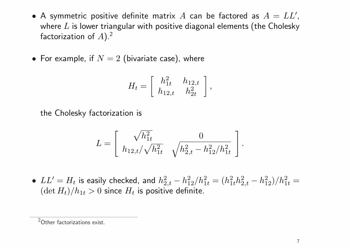
• A symmetric positive definite matrix A can be factored as A = LL′,where L is lower triangular with positive diagonal elements (the Choleskyfactorization of A).2

• For example, if N = 2 (bivariate case), where

Ht =[

h21t h12,t

h12,t h22t

],

the Cholesky factorization is

L =

[ √h2

1t 0

h12,t/√

h21t

√h2

2,t − h212/h2

1t

].

• LL′ = Ht is easily checked, and h22,t − h2

12/h21t = (h2

1th22,t − h2

12)/h21t =

(det Ht)/h1t > 0 since Ht is positive definite.

2Other factorizations exist.

7

• It then follows from (8) that

Vart−1(rt) = Vart−1(εt) (9)

= Et−1(εtε′t)− Et−1(εt)︸ ︷︷ ︸

=0

Et−1(εt)′ (10)

= Et−1(H1/2t ztz

′t(H

1/2t )′) (11)

= H1/2t Et−1(ztz

′t)︸ ︷︷ ︸

=identity matrix

(H1/2t )′ (12)

= H1/2t (H1/2

t )′ = Ht. (13)

8

Main Problems

• There are two main problems when it comes to the specification ofmultivariate GARCH models:

(i) To keep estimation feasible, we need parsimonious models (i.e., modelswith a moderate number of parameters) which are still flexible enough tocapture the most important aspects of the volatility/covariance dynamics.

(ii) We have to make sure that the conditional covariance matrix will remainpositive definite at each point of time.

• For the sake of illustration, consider a bivariate GARCH(1,1) of thegeneral vec–type.

• The covariance matrix is then given by

Ht =[

h21t h12,t

h12,t h22t

],

9

where, in the most general case

h21t = c1 + a11ε

21,t−1 + a12ε1,t−1ε2,t−1 + a13ε

22,t−1

+b11h21,t−1 + b12h12,t−1 + b13h

22,t−1

h12,t = c2 + a21ε21,t−1 + a22ε1,t−1ε2,t−1 + a23ε

22,t−1

+b21h21,t−1 + b22h12,t−1 + b23h

22,t−1

h22t = c3 + a31ε

21,t−1 + a32ε1,t−1ε2,t−1 + a33ε

22,t−1

+b31h21,t−1 + b32h12,t−1 + b33h

22,t−1,

or

h21,t

h12,t

h22,t

︸ ︷︷ ︸=ht

=

c1

c2

c3

+

a11 a12 a13

a21 a22 a23

a31 a32 a33

ε21,t−1

ε1,t−1ε2,t−1

ε22,t−1

+

b11 b12 b13

b21 b22 b23

b31 b32 b33

h21,t−1

h12,t−1

h22,t−1

.

10

• In this specification, both conditional variances, h21t and h2

2t, and theconditional covariance, h12,t, may depend on all lagged squared returnsand variances and all lagged cross–products ε1,t−1ε2,t−1 and covariances.

• Although flexible, this model is difficult to handle in practice, since itrequires estimation of 21 parameters (and this is for the bivariate case).

• Moreover, without further restrictions, there is no guarantee that thesequence of covariance matrices implied by an estimated process will bepositive definite for all t.

• Such conditions are very tedious to work out and to impose in estimation.

• The system above is a bivariate version of the vec model, which is astraightforward generalization of univariate GARCH.

• The general case is still useful, as it nests many more practicablespecifications.

11

• The name derives from the fact that it uses the vech operator.

• As the N × N matrix Ht is symmetric, it contains only N(N + 1)/2independent elements, which may be obtained, for example, by excludingthe upper triangular (redundant) part.

• The vech operator then stacks the remaining elements columnwise intoan N(N + 1)/2 column vector, e.g.,

vech([

h21t h12,t

h12,t h22t

])=

h21t

h12,t

h22t

vech(εtε′t) = vech

([ε1t

ε2t

] [ε1t ε2t

])

= vech([

ε21t ε1tε2t

ε1tε2t ε22t

])=

ε21t

ε1tε2t

ε22t

.

• The vec operator is similar, but without excluding the upper triangularpart.

12

• Then the vec(1,1) model can be written

ht = c + Aηt−1 + Bht−1, (14)

where

ht = vechHt (15)

ηt = vech(εtε′t). (16)

• Without restrictions, the are

– N(N + 1)/2 parameters in c– N2(N + 1)2/4 parameters in A– N2(N + 1)2/4 parameters in B.– With N = 2, 3, 5, 10 assets, we have 21, 78, 465, 6105 parameters.

13

Stationarity and Unconditional Variance

• The covariance stationarity for the vec(1,1) model (14),

ht = c + Aηt−1 + Bht−1, (17)

requires the eigenvalues of matrix

Q = A + B

to be inside the unit circle.

• If this holds, the unconditional covariance matrix (its vech) can beobtained by taking expectations on both sides of (17),

E(ht) = c + AE(ηt−1) + BE(ht−1)

= c + AE(ht−1) + BE(ht−1)

= c + (A + B)E(ht),

14

henceE(vechHt) = E(ht) = (I −A−B)−1

c.

• Covariance matrix forecasts:

ht+1 = c + Aηt + Bht

Et(ht+2) = c + AEtηt+1 + Bht+1 = c + (A + B)ht+1

Et(ht+3) = c + AEtηt+2 + BEtht+2

= c + (A + B)Etht+2 = c + (A + B)c + (A + B)2ht+1

...

Et(ht+τ) =τ−2∑

i=0

(A + B)ic + (A + B)τ−1ht+1

= E(ht) + (A + B)τ−1(ht+1 − E(ht)),

usingτ−2∑

i=0

(A + B)i = [I − (A + B)τ−1](I −A−B)−1.

15

• Et(ht+τ) converges to the unconditional covariance matrix provided thecovariance stationarity condition is satisfied.

• Calculation of higher moments of the vec model is considerably moreinvolved than in the univariate GARCH model.3

3C. M. Hafner (2003): Fourth Moment Structure of Multivariate GARCH Models, Journal of FinancialEconometrics, 1, 26–54.

16

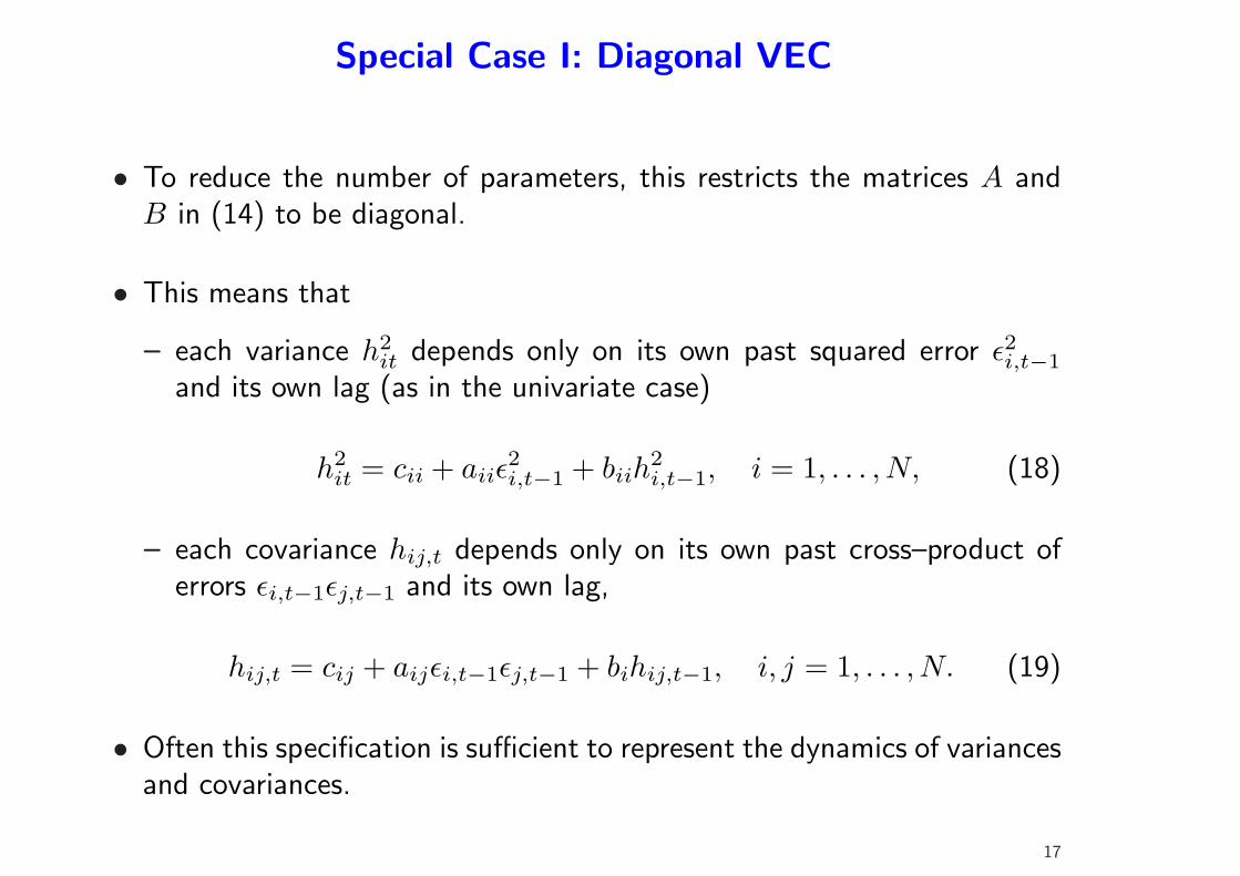
Special Case I: Diagonal VEC

• To reduce the number of parameters, this restricts the matrices A andB in (14) to be diagonal.

• This means that

– each variance h2it depends only on its own past squared error ε2i,t−1

and its own lag (as in the univariate case)

h2it = cii + aiiε

2i,t−1 + biih

2i,t−1, i = 1, . . . , N, (18)

– each covariance hij,t depends only on its own past cross–product oferrors εi,t−1εj,t−1 and its own lag,

hij,t = cij + aijεi,t−1εj,t−1 + bihij,t−1, i, j = 1, . . . , N. (19)

• Often this specification is sufficient to represent the dynamics of variancesand covariances.

17

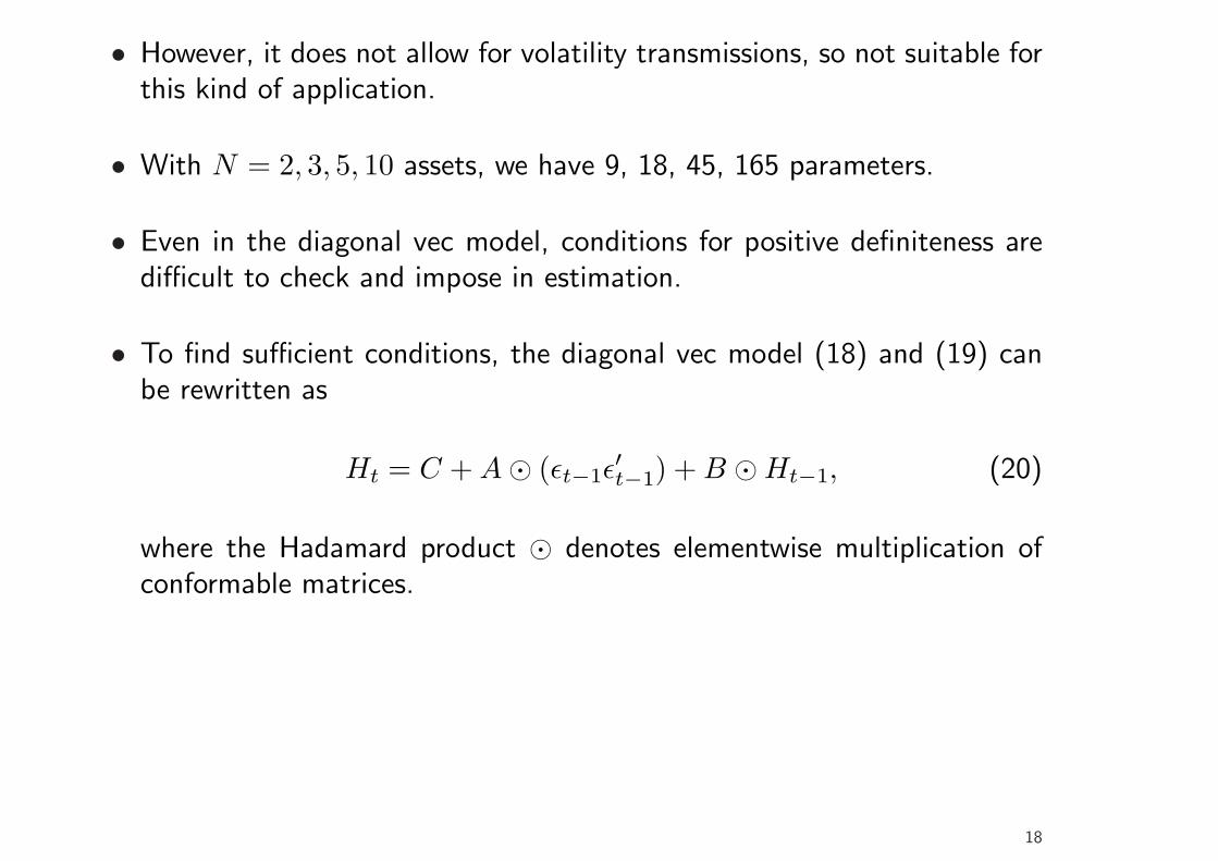
• However, it does not allow for volatility transmissions, so not suitable forthis kind of application.

• With N = 2, 3, 5, 10 assets, we have 9, 18, 45, 165 parameters.

• Even in the diagonal vec model, conditions for positive definiteness aredifficult to check and impose in estimation.

• To find sufficient conditions, the diagonal vec model (18) and (19) canbe rewritten as

Ht = C + A¯ (εt−1ε′t−1) + B ¯Ht−1, (20)

where the Hadamard product ¯ denotes elementwise multiplication ofconformable matrices.

18

• E.g., for N = 2,

[h2

1t h12,t

h12,t h22t

]=

[c11 c12

c12 c22

]+

[a11 a12

a12 a22

]¯

[ε21,t−1 ε1,t−1ε2,t−1

ε1,t−1ε2,t−1 ε22,t−1

]

+[

b11 b12

b12 b22

]¯

[h2

1,t−1 h12,t−1

h12,t−1 h22,t−1

].

19

Schur product theorem

• Consider two normally distributed zero–mean random vectors X and Y(of the same length), where

– X has covariance matrix ΣX, and– Y has covariance matrix ΣY ,

and X and Y are independent.

• Now consider the product X ¯ Y .

• The covariance between the ith and jth elements of X ¯ Y is

Cov(Xi · Yi, Xj · Yj) = E(XiYiXjYj)− E(XiYi)E(XjYj)independence

= E(XiXj)E(YiYj)− E(Xi)E(Yi)E(Xj)E(Yj)zero mean= E(XiXj)E(YiYj)

= Cov(Xi, Xj)Cov(Yi, Yj).

20

• It follows that the covariance matrix of X ¯ Y is ΣX ¯ ΣY .

• Thus ΣX ¯ ΣY is a covariance matrix and therefore positive definite.

• Since any positive definite matrix is the covariance matrix of a normalrandom vector we conclude that the Hadamard product of two positivedefinite matrices is likewise positive definite.

• This result is often referred to as the Schur product theorem.4

4Which is slightly more general, allowing also for positive semi–definite matrices.

21

• The Schur product theorem can be applied to the representation5

Ht = C + A¯ (εt−1ε′t−1) + B ¯Ht−1 (21)

to conclude that

– if (symmetric) matrices C, A, and B are positive definite (or indeedsemi–definite), and

– the initial covariance matrix H0 is positive definite,

then Ht will remain positive definite for all t.

• During estimation, matrices C, A, and B can be parameterized in termsof their Cholesky factorization to guarantee positive semi–definiteness.i.e., one estimates the system

Ht = CC ′ + AA′ ¯ (εt−1ε′t−1) + BB′ ¯Ht−1, (22)

where A, B, and C are lower triangular with positive diagonal.5Cf. Z. Ding and R. F. Engle (2001): Large Scale Conditional Covariance Matrix Modeling, Estimation

and Testing, Academia Economic Papers, 29, 157–184.

22

• For high–dimensional systems, it is still not feasible to estimate (22)directly.

• Two ways to proceed:

(i) Introduce further simplifications.(ii) Keep the full flexibility of the diagonal vec model and use a clever

estimation method, as in Ledoit et al. (2003).6

• Briefly, as to (i), the most extreme case is the scalar–diagonal model,given by

Ht = CC ′ + αεt−1ε′t−1 + βHt−1, (23)

where α and β are positive scalars.

• We can do variance targeting by noting that the unconditionalcovariance matrix in (23) is CC ′/(1− α− β).

6O. Ledoit, P. Santa–Clara and M. Wolf, Flexible Multivariate GARCH Modeling with an Application toInternational Stock Markets, Review of Economics and Statistics, 85, 735–747.

23

• Thus, we may put

Ht = S(1− α− β) + αεt−1ε′t−1 + βHt−1, (24)

where S is the sample covariance matrix (or any long–run covariancematrix imposed by the analyst).

• Thus only two parameters need to be estimated numerically.7

• Clearly this is a very restrictive model, as it assumes the same kind ofvolatility dynamics to be present in each asset.

• A practically relevant example of (23), where β = 1 − α = λ, is theexponentially weighted moving average (EWMA), where

Ht = λHt−1 + (1− λ)εt−1ε′t−1 = (1− λ)

∞∑

i=1

λi−1εt−iε′t−i,

where λ is fixed at 0.94 for daily data in the RiskMetrics model.

7The long–run covariance matrix is of course also an estimate, but it need not be estimated numerically.

24

• As to (ii), we can estimate high–dimensional systems by applying themethodology suggested by Ledoit et al. (2003).

• The idea is to first obtain each set of coefficient estimates cij, bij, andcij separately for each pair of assets (i, j).

• This can be achieved simply by estimating one– or two–dimensionalGARCH models for the conditional variances and covariances respectively.

• That is, in the first step, for all individual return series, we fit a univariateGARCH model to get coefficient estimates cii, aii, and bii, i = 1, . . . , N .

• We use these estimates to calculate a sequence of conditional varianceestimates, h2

it, for each asset,

h2it = cii + aiiε

2i,t−1 + biih

2i,t−1, t = 1, . . . , T, i = 1, . . . , N. (25)

25

• In the second stage, the estimates (25) are used to specify bivariatelikelihood functions for the off-diagonal elements. For example, ifnormality is assumed, we maximize

−12

T∑t=1

(log |Hij,t|+ 1

2ε′ij,tH

−1ij,tεij,t

),

where

εij,t =[

εit

εjt

], Hij,t =

[h2

it hij,t

hij,t h2jt

],

h2it and h2

jt are from (25), and the diagonal vec GARCH specification forthe conditional covariance

h2ij,t = cij + aijεi,t−1εj,t−1 + bijhij,t−1 (26)

i, j = 1, 2, . . . , N, i 6= j. (27)

• In each of these second–step bivariate problems, only three parametersin (26) have to be estimated.

26

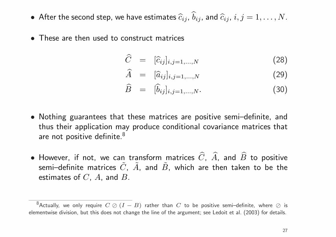
• After the second step, we have estimates cij, bij, and cij, i, j = 1, . . . , N .

• These are then used to construct matrices

C = [cij]i,j=1,...,N (28)

A = [aij]i,j=1,...,N (29)

B = [bij]i,j=1,...,N . (30)

• Nothing guarantees that these matrices are positive semi–definite, andthus their application may produce conditional covariance matrices thatare not positive definite.8

• However, if not, we can transform matrices C, A, and B to positivesemi–definite matrices C, A, and B, which are then taken to be theestimates of C, A, and B.

8Actually, we only require C ® (I − B) rather than C to be positive semi–definite, where ® iselementwise division, but this does not change the line of the argument; see Ledoit et al. (2003) for details.

27

• Matrices C, A, and B are chosen such that they are positive semi–definitematrices and as close as possible to C, A, and B in the Frobenius norm,9

i.e., by minimizing ‖C − C‖F , ‖A − A‖F , and ‖B − B‖F , where forN ×N matrix M ,10

‖M‖F =

√√√√N∑

i=1

N∑

j=1

m2ij.

• Ledoit et al. (2003) show that this works well in applications to volatilityforecasting, Value–at–Risk measurement, and portfolio selection.

9In addition, it is imposed that the diagonal elements do not change.10Matlab code for doing the optimization is available at

http://www.iew.uzh.ch/institute/people/wolf/publications.html.

28

Special Case II: BEKK

• BEKK (Baba, Engle, Kraft, and Kroner) was suggested by Engle andKroner (1995).11

• This specifies, in its simplest form,

Ht = C?C?′ + A?εt−1ε′t−1A

?′ + B?Ht−1B?′, (31)

where C is a triangular matrix and A? and B? are N × N parametermatrices.

• This guarantees positive definiteness if the initialization of Ht is positivedefinite.

• So the number of parameters is N(5N + 1)/2, i.e., for N = 2, 3, 5, 10assets, we have 11, 24, 65, 255 parameters.

11Multivariate Simultaneous Generalized ARCH, Econometric Theory, 11, 122–150.

29

• To see that this is a restricted vec model, consider the case N = 2,where

[h2

1t h12,t

h12,t h22,t

]=

[c?11 0

c?21 c?

22

] [c?11 c?

21

0 c?22

]

+[

a?11 a?

12

a?21 a?

22

] [ε21,t−1 ε1,t−1ε2,t−1

ε1,t−1ε2,t−1 ε22,t−1

] [a?11 a?

12

a?21 a?

22

]′

+[

b?11 b?

12

b?21 b?

22

] [h2

1,t−1 h12,t−1

h12,t−1 h22,t−1

] [b?11 b?

12

b?21 b?

22

]′,

or

h21,t = c1 + a?2

11ε21,t−1 + 2a?

11a?12ε1,t−1ε2,t−1 + a?2

12ε22,t−1

+b?211h

21,t−1 + 2b?

11b?12h12,t−1 + b?2

12h22,t−1

h12,t = c2 + a?11a

?21ε

21,t−1 + (a?

11a?22 + a?

21a?12)ε1,t−1ε2,t−1 + a?

22a?12ε

22,t−1

+b?11b

?21h

21,t−1 + (b?

11b?22 + b?

12b?21)h12,t−1 + b?

22b?12h

22,t−1.

30

• For the general relation between the models, the Kronecker product ⊗turns out to be useful.

• For an m × n matrix A and an p × q matrix B, this is defined as themp× nq matrix

A⊗B =

a11B a12B · · · a1nBa21B a22B · · · a2nB

... ... . . . ...am1B am2B · · · amnB

.

• Important rule in time series analysis:

vec(ABC) = (C ′ ⊗A)vec(B).

• Then (31) can be written as

vec(Ht) = vec(C?C?′)+(A?⊗A?)vec(εt−1ε′t−1)+(B?⊗B?)vec(Ht−1).

(32)

31

• Representation (32) directly leads to stationarity conditions andcovariance matrix forecasts for the BEKK model.

• In practice, the diagonal BEKK model is sometimes used to furtherreduce the number of parameters to be estimated, where the parametermatrices A? and B? are diagonal.

32

Factor Models

• Basic idea: Co–movements of returns are driven by a small number of(observable or unobservable) common underlying variables, which arecalled factors.

• For example, as an observable factor, the return of a market index maybe used as a proxy for the general tendency of the stock market.

• Consider the simplest case of just a single observable factor.

• Think of this as the market return, denoted by rMt.

• In portfolio analysis, where factor models are often used to structurecovariance matrices, the model is also known as single index model(SIM).

33

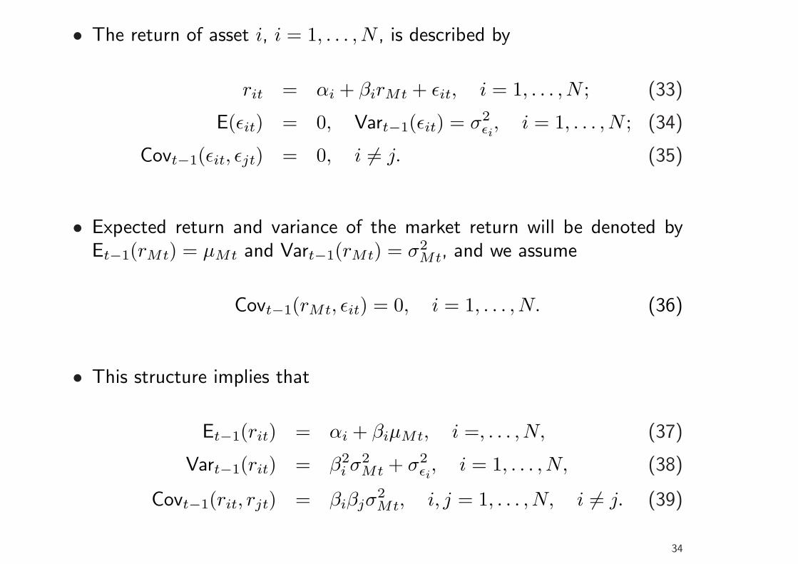
• The return of asset i, i = 1, . . . , N , is described by

rit = αi + βirMt + εit, i = 1, . . . , N ; (33)

E(εit) = 0, Vart−1(εit) = σ2εi, i = 1, . . . , N ; (34)

Covt−1(εit, εjt) = 0, i 6= j. (35)

• Expected return and variance of the market return will be denoted byEt−1(rMt) = µMt and Vart−1(rMt) = σ2

Mt, and we assume

Covt−1(rMt, εit) = 0, i = 1, . . . , N. (36)

• This structure implies that

Et−1(rit) = αi + βiµMt, i =, . . . , N, (37)

Vart−1(rit) = β2i σ2

Mt + σ2εi, i = 1, . . . , N, (38)

Covt−1(rit, rjt) = βiβjσ2Mt, i, j = 1, . . . , N, i 6= j. (39)

34

• For the covariance structure of the returns, given by (39), Assumption(35) is crucial, as it implies that the only reason for asset i and asset jmoving together is their joint dependence on the market return rMt.

• The first part of (38) is also often referred to as the systematic risk(which is related to the general tendency of the market), whereas thesecond part is the unsystematic (idiosyncratic, specific) risk, which is notrelated to market factors.

• The conditional variance of the market factor can be modeled by meansof a univariate (asymmetric) (E)GARCH model, e.g.,

σ2Mt = c + aε2M,t−1 + bσ2

M,t−1, (40)

whereεMt = rMt − µMt. (41)

• Equation (38) implies that the GARCH effects in the market will betransferred to all the assets’ variances.

35

• Defining

β =

β1

β2...

βN

, Σε =

σ2ε1

0 · · · 00 σ2

ε2· · · 0

... ... . . . ...0 0 · · · σ2

εN

,

the conditional covariance matrix of the N–dimensional rt =[r1t, r2t, . . . , rNt]′ can be written as

Covt−1(rt) =

β21σ

2Mt + σ2

ε1β1β2σ

2Mt · · · β1βNσ2

Mt

β1β2σ2Mt β2

2σ2Mt + σ2

ε2· · · β2βNσMt

... ... . . . ...β1βNσ2

Mt β2βNσ2Mt · · · β2

Nσ2Mt + σ2

εN

= ββ′σ2Mt + Σε.

36

Modeling Conditional Correlations

• The models considered so far specified models for the conditionalcovariances, in addition to the variances.

• Another approach is to model the variances and the conditionalcorrelations.

• One advantage is that conditional variances (or standard deviations) andconditional correlations can be modeled separately, which often allows forconsistent two–step model estimation, thus reducing the computationalburden.

• For these models, we write Ht as

Ht = DtRtDt (42)

Dt =

√h2

1t 0 · · · 00

√h2

2t · · · 0... ... . . . ...

0 0 · · ·√

h2Nt

, (43)

37

i.e., Ht is a diagonal matrix with the conditional standard deviations onits main diagonal, and

Rt =

1 ρ12,t · · · ρ1N,t

ρ12,t 1 · · · ρ2N,t... ... . . . ...

ρ1N,t ρ2N,t · · · 1

(44)

is the conditional correlation matrix, i.e.,

ρij,t = Corrt−1(εit, εjt), i, j = 1, . . . , N, i 6= j,

is the conditional correlation between assets i and j.

• The conditional covariances are

hij,t = ρij,t

√h2

ith2jt, i 6= j.

• Positive definiteness of Ht follows from that of Rt and the positivity ofthe conditional standard deviations in Dt.

38

Constant Conditional Correlations (CCC)

• One of the first multivariate GARCH models (Bollerslev, 1990).12

• In this model Rt = R is constant in (42), i.e., the conditional correlationsare constant.

• We may write this asεt = Dtzt, (45)

where {(z1t, . . . , zNt)′} is an iid series of (e.g., normally distributed)innovations with mean zero and covariance matrix R, i.e.,

zt ∼ N(0, R). (46)

• Until ten years ago or so, it has also been the most popular multivariateGARCH model due to the fact that it can easily be estimated even forhigh–dimensional time series.

12Modelling the coherence in short–run nominal exchange rates: a multivariate generalized ARCH model,Review of Economics and Statistics, 73, 498–505.

39

• Note that R is the constant conditional correlation matrix (i.e., thecorrelation matrix of the innovations), not the unconditional correlationmatrix.

• Consistent two–step estimation for high–dimensional time series feasible:

• First estimate univariate GARCH models for each series.

• This allows for flexible specification of the univariate processes. Forexample, we may specify a standard GARCH for one component,AGARCH or EGARCH for another...

• Calculate the standardized residuals,

zit =εit√h2

it

, i = 1, . . . , N, t = 1, . . . , T. (47)

• Then, in view of (45) and (45), estimate R as the correlation matrix ofthe standardized residuals.

40

• The CCC has been extended to allow for volatility spillovers by specifyinga multivariate GARCH structure for the conditional volatilities of theindividual series.13

• For the bivariate case, this is

[h2

1t

h22t

]=

[c1

c2

]+

[a11 a12

a21 a22

] [ε21,t−1

ε22,t−1

]+

[b11 b12

b21 b22

] [h2

1t

h22t

].

• This allows past squared returns and variances of all series to enter theindividual conditional variance equations.

• This clearly requires simultaneous estimation of the conditional varianceparameters on the first step.

13T. Jeantheau (1998): Strong consistency of estimators for multivariate ARCH models, EconometricTheory, 14, 70–86; C. He and T. Terasvirta (2004): An extended constant conditional correlation GARCHmodel and its fourth–moment structure, Econometric Theory, 20, 904–926.

41

Dynamic Conditional Correlation (DCC) Models

• The two–step estimation procedure makes application of the CCCto high–dimensional systems feasible, but more often than not thehypothesis of constant conditional correlations is rejected.

• For example, it is often observed that correlations between financial timeseries increase in turbulent periods, and are very high in crash situations.

• Thus models for dynamic conditional correlations (DCC) have beenproposed.

• As an example, consider the model proposed by Engle (2002).14

14Dynamic conditional correlation—a simple class of multivariate GARCH model, Journal of Business andEconomic Statistics, 20, 339–350. A similar model was suggested by Y. K. Tse and A. K. C. Tsui (2002): Amultivariate GARCH model with time–varying correlations, Journal of Business and Economic Statistics, 20,351–362.

42

• In its simplest (scalar) form, this can be written as

εt ∼ N(0, DtRtDt), (48)

Dt ∼ GARCH (49)

zt = D−1εt (produces standardized residuals (47))

Qt = (1− a− b)S + azt−1z′t−1 + bQt−1, (50)

a, b ≥ 0, a + b < 1,

Rt = {diag(Qt)}−1/2Qt{diag(Qt)}−1/2. (51)

• In (50), S is the unconditional correlation matrix of the standardizesresiduals zt.

• If the starting value for Qt in (50) is positive definite, then Qt is positivedefinite, but will not in general be a valid correlation matrix (i.e., withones on the diagonal).

• Thus, the rescaling in (51) is necessary.

43

• Two–step estimation is still feasible, which facilitates the application totime series of higher dimension.

• More general GARCH–like structures than the scalar model in (50) canbe employed.

• An alternative multivariate GARCH model for dynamic conditionalcorrelations was suggested by Pelletier (2006), i.e., a regime-switchingmodel for dynamic correlations.15

• In Pelletier’s (2006) model, the conditional correlation matrix is subjectto Markovian regime–switching and is given by

R(∆t) = [ρij(∆t)], i, j = 1, . . . , M, (52)

where {∆t} is a Markov chain with finite state space S = {1, . . . , k} and

15D. Pelletier (2006): Regime–switching for Dynamic Correlations, Journal of Econometrics, 131, 445–473.

44

irreducible and aperiodic (primitive) transition matrix

P =

p11 · · · pk1... · · · ...

p1k · · · pkk

, (53)

where pij = p(∆t = j|∆t−1 = i), i, j = 1, . . . , k.

45

• In principle, any volatility model can be employed for generating thevolatility dynamics of the individual assets. However, Pelletier assumesthat an absolute value GARCH(1,1) (AVGARCH) process is appropriate,i.e.,

εi,t = zithit, (54)

hit = ωi + αi|εi,t−1|+ βihi,t−1 (55)

= ωi + αi|zi,t−1|hi,t−1 + βihi,t−1 (56)

= ωi + (αi|zi,t−1|+ βi)hi,t−1 (57)

= ωi + ci,t−1hi,t−1, (58)

ωi > 0, αi, βi ≥ 0, i = 1, . . . , N,

wherecit = αi|zi,t|+ βi,

and where the volatility dynamics are specified in terms of the conditionalstandard deviation.

• The reason for doing so is that this allows for closed–form covariancematrix forecasts.

46

• This is not the case for the constant conditional correlation model wherethe volatility dynamics are specified in terms of the conditional variance.

• To see this, consider the standard model with a single regime only.

• The forecast of the time–t conditional covariance between asset 1 andasset 2 at time t + d is given by

Covt(ε1,t+d, ε2,t+d) = Et(ε1,t+d, ε2,t+d) = Et(z1,t+dz2,t+dh1,t+dh2,t+d)

= E(z1,t+dz2,t+d)︸ ︷︷ ︸=ρ12

Et(h1,t+dh2,t+d)

= ρ12Et(h1,t+dh2,t+d).

• Now we can substitute for h1,t+d and h2,t+d to obtain

h1,t+dh2,t+d = (ω1 + c1,t+d−1h1,t+d−1)(ω2 + c2,t+d−1h2,t+d−1)

= ω1ω2 + ω1c2,t+d−1h2,t+d−1 + ω2c1,t+d−1h1,t+d−1

+c1,t+d−1c2,t+d−1h1,t+d−1h2,t+d−1.

47

• Defining

st = ω1ω2 + ω1c2,th2,t + ω2c1,th1,t, c12,t = c1tc2t,

this can be written

h1,t+dh2,t+d = st+d−1 + c12,t+d−1h1,t+d−1h2,t+d−1,

and taking conditional expectations gives

Et(h1,t+dh2,t+d) = Et(st+d−1) + c12Et(h1,t+d−1h2,t+d−1), (59)

where c12 = E(c1tc2t).

• Et(st+d−1) in (59) can be calculated via the GARCH(1,1) volatilityforecast formula

Et(hi,t+τ) = ω11− cτ−1

i

1− ci+cτ−1

i hi,t+1 = E(hit)+cτ−1i (hi,t+1−E(hit)), τ ≥ 1,

48

where E(hit) = ωi(1− ci)−1, ci = E(cit) = αiκ1 + βi, i = 1, 2, and

κ1 = E(|zit|) =

√2π if zit ∼ N(0, 1)

√ν−2Γ(ν−1

2 )√πΓ(ν/2)

if zit ∼ tν,(60)

where tν denotes Student’s t distribution with ν > 2 degrees of freedomand unit variance.

• Furthermore

c12 = E(c1tc2t) = α1α2E(|z1tz2t|) + κ1(α1β2 + α2β1) + β1β2,

where16

E(|z1tz2t|) =2π

(ρ12 arcsin ρ12 +

√1− ρ2

12

)

both for normal as well as Student’s t innovations.17

16S. Nabeya (1951): Absolute Moments in 2–dimensional Normal Distribution, Annals of the Institute ofStatistical Mathematics, 3, 2–6.

17Provided the Student distribution has been standardized to have unit variance.

49

• Now we can iterate (59) to obtain

Et(h1,t+dh2,t+d) = Et(st+d−1) + c12Et(h1,t+d−1h2,t+d−1)

= Et(st+d−1) + c12Et(st+d−2) + c212Et(h1,t+d−2h2,t+d−2)

...

=d−2∑

`=0

c`12Et(st+d−`−1) + cd−1

12 h1,t+1h2,t+1.

• On the other hand, using a GARCH model in the variance and thesquared returns, calculation of covariance matrix forecasts would requirethe evaluation of

Covt(ε1,t+d, ε2,t+d) = ρ12Et (h1,t+dh2,t+d) ,

where

hi,t+d =√

ωi + (αiz2i,t+d−1 + βi)h2

i,t+d−1, i = 1, 2,

which does not allow a closed–form solution.

50

• To illustrate the application of the model, we consider dynamiccorrelations between global stock market and real estate equity returns,using dollar–denominated weekly (Wednesday–to–Wednesday) returns ofthe MSCI world and the FTSE EPRA/NAREIT global indices over theperiod from January 1990 to May 2009 (T = 1012 observations).

• Continuously compounded percentage returns are considered, i.e.,

rit = 100× log(Iit/Ii,t−1), i = 1, 2,

where I1t and I2t are the MSCI and EPRA/NAREIT index levels at timet, respectively.

51

1990 1992 1994 1996 1998 2000 2002 2004 2006 2008 201050

100

150

200

250

300Index

stock marketreal estate

52

1990 1992 1994 1996 1998 2000 2002 2004 2006 2008 2010−20

−15

−10

−5

0

5

10stock market returns

1990 1992 1994 1996 1998 2000 2002 2004 2006 2008 2010−30

−20

−10

0

10

20real estate returns

53

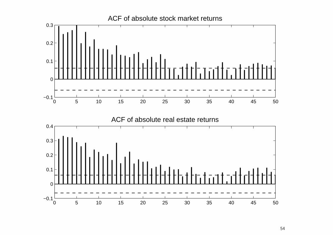
0 5 10 15 20 25 30 35 40 45 50−0.1

0

0.1

0.2

0.3ACF of absolute stock market returns

0 5 10 15 20 25 30 35 40 45 50−0.1

0

0.1

0.2

0.3

0.4ACF of absolute real estate returns

54

Table 1: Properties of stock market and real estate returns

covariance/

mean correlation matrix skewness kurtosis JB

MSCI 0.051 4.806 0.768 −0.794 8.060 1186.1∗∗∗

EPRA/NAREIT 0.019 4.242 6.346 −1.239 12.49 4053.3∗∗∗

• JB is the Jarque–Bera test for normality.

55

• Estimate models with one and two regimes, and with normal andStudent’s t innovations.

• First compare standard GARCH (i.e., modeling conditional variances)with absolute value GARCH (AVGARCH, i.e., modeling conditionalstandard devations).

• Although models based on squared returns do slightly better than thoseusing absolute values for Gaussian innovations, there are basically nodifferences for Student’s t models.

• Clearly, as the latter lead to a much better fit than the former, resultspertaining to them appear to be more informative.

• We also note that allowing for regime–dependent correlations in generalsubstantially decreases the BIC, providing strong support for time–varyingcorrelations.

56

Table 2: Likelihood–based goodness–of–fitAVGARCH models

Gaussian Student’s t

k = 1 k = 2 k = 1 k = 2

K 9 12 10 13

log L −3877.9 −3843.6 −3832.5 −3806.0

BIC 7818.1 7770.1 7734.3 7702.0

GARCH models

Gaussian Student’s t

k = 1 k = 2 k = 1 k = 2

K 9 12 10 13

log L −3874.6 −3841.5 −3832.5 −3806.7

BIC 7811.6 7765.9 7734.2 7703.3Reported are likelihood–based goodness–of–fit measures for variousbivariate GARCH models fitted to the international stock and realestate equity markets. AVGARCH indicates Taylor’s (1986) absolutevalue GARCH process for the individual volatilities, as given by (55),whereas GARCH is the specification of Bollerslev (1986), where (55) isreplaced by h2

it = ωi + αiε2i,t−1 + βih

2i,t−1, i = 1, 2. K denotes

the number of parameters of a model, log L is the value of themaximized log–likelihood, and BIC is the Bayesian information criterion,i.e., BIC = −2× log L + K log T , where T is the sample size.

57

Table 3: Parameter estimates for AVGARCH modelsGaussian Student’s t

k = 1 k = 2 k = 1 k = 2

ω1 0.054(0.020)

0.058(0.019)

0.043(0.018)

0.041(0.017)

α1 0.094(0.016)

0.100(0.016)

0.080(0.016)

0.086(0.016)

β1 0.901(0.021)

0.893(0.020)

0.918(0.019)

0.914(0.018)

ω2 0.085(0.028)

0.054(0.019)

0.057(0.024)

0.036(0.017)

α2 0.088(0.015)

0.088(0.013)

0.076(0.015)

0.080(0.014)

β2 0.896(0.023)

0.910(0.017)

0.916(0.021)

0.924(0.016)

ρ12(1) 0.747(0.014)

0.654(0.029)

0.745(0.016)

0.669(0.025)

ρ12(2) − 0.913(0.013)

− 0.894(0.013)

ν − − 7.257(1.048)

7.286(1.052)

P 1

0.964(0.019)

0.066(0.029)

0.036(0.019)

0.934(0.029)

1

0.994(0.004)

0.010(0.009)

0.006(0.004)

0.990(0.009)

π1,∞ 1 0.649 1 0.645

(1− p11)−1 ∞ 28.12 ∞ 181.2

(1− p22)−1 − 15.21 − 99.67

58

• In the Gaussian regime–switching model model, expected regime

durations, (1 − pjj)−1, j = 1, 2, are only 28 and 15 weeks for the

low– and the high–correlation regime.

• They are approximately 3.5 years and two years in the Student’s t model.

59

60

1990 1995 2000 2005 20100

0.1

0.2

0.3

0.4

0.5

0.6

0.7

0.8

0.9

1Gaussian

time

smoo

thed

pro

b. o

f reg

ime

2

1990 1995 2000 2005 20100

0.1

0.2

0.3

0.4

0.5

0.6

0.7

0.8

0.9

1Student´s t

timesm

ooth

ed p

rob.

of r

egim

e 2

1 25 50 75 1000.65

0.7

0.75

0.8

0.85

0.9

forecast horizon, d

(con

ditio

nal)

corr

elat

ion

Gaussian

π1t

= 1

π2t

= 1

unconditional correlation

1 50 100 150 200 250 3000.65

0.7

0.75

0.8

0.85

0.9

forecast horizon, d

(con

ditio

nal)

corr

elat

ion

Student´s t

π1t

= 1

π2t

= 1

unconditional correlation

61

• In view of these differences between regime–switching models based

on different distributions, we shall investigate their consequences for

out–of–sample forecasting.

• To this end, we first reestimate the models using the first 500 observations

and then update the estimates every four weeks, using an expanding

window of data.

• We use the estimates to construct ex–ante global minimum variance

portfolios (GMVP) for (cumulative) returns at forecast horizons D =1, 4, 8, 12, 16, 20, and 24.

• As pointed out by Ledoit et al. (2003), an advantage of using the GMVP

is that it allows us to refrain from specifying expected returns, “which is

more a task for the portfolio manager than a statistical problem”.

62

• In general, for a portfolio of N assets with weight vector w =[w1, w2, . . . , wN ], the portfolio mean and variance are given by

µp = w′µ, and σ2p = w′Hw,

where µ and H are the mean vector and covariance matrix, respectively,

of the assets under study.

• A minimum variance (well diversified) portfolio is a portfolio that

minimizes the variance for a prespecified level of expected portfolio

return, µ?p, i.e.,

min σ2p = w′Hw, subject to µp = w′µ ≥ µ?

p. (61)

• Once we restrict our attention to efficient minimum variance portfolios,18

a higher expected return can only be achieved by accepting a higher

variance, i.e., we trade off risk for expected return.18These have maximum expected return for a given variance.

63

• However, the optimal risk–return combination depends on the preferences

of the investor, and it involves expected returns, which are much harder

to estimate statistically than volatilities and covariances.

• Thus, in covariance matrix forecasts are of interest, one often

concentrates on the GMVP, which is the portfolio that solves (61)

without any restrictions on the portfolio mean return.

• For two assets, with w being the weight of the first asset, portfolio

variance h2p is

h2p = w2h2

1 + (1− w)2h22 + 2w(1− w)h12 (62)

= w2(h21 + h2

2 − 2h12)− 2w(h22 − h12) + h2

2.

• The GMVP is obtained by minimizing (62), i.e.,

wGMVP =h2

2 − h12

h21 + h2

2 − 2h12.

64

• For the Gaussian CCC, we report the standard deviation of the realized

returns, whereas for the other models their respective standard deviation

divided by that of the Gaussian CCC is indicated.

• Compared to the latter, the improvements from switching to a Student’s

t distribution are generally small.

• Those from using a regime–switching model for the correlations are

larger, although still moderate for shorter forecast horizons.

• However, as D becomes larger, the relative performance of the regime–

switching approach improves considerably, but only for the Student’s t

model.

• This is very likely due to the fact that, at longer forecast horizons, the

higher persistence of the correlation regimes implied by the Student’s

t model becomes effective, whereas the conditional correlation of the

Gaussian model rapidly converges to its unconditional value.

65

Table 4: Properties of realized global minimum variance portfolio (GMVP)

returnsD 1 4 8 12 16 20 24

Gaussian CCC 2.314 4.994 7.660 9.222 10.89 12.96 15.03

Student’s t CCC 0.997 0.994 0.989 0.992 0.991 0.987 0.985

Gaussian regime–switching 0.978 0.970 0.962 0.970 0.970 0.963 0.965

Student’s t regime–switching 0.968 0.954 0.929 0.925 0.925 0.919 0.917Shown are the results from calculating ex–ante global minimum variance portfolios (GMVP) implied by different

GARCH models and for different forecast horizons. For the Gaussian CCC, we show, for each forecast horizon,

D, the standard deviation of realized returns resulting from ex–ante GMVP portfolio weights. For the other

models, we report their respective standard deviation divided by that of the Gaussian CCC. The first row of

the table specifies the forecast horizon, D. The calculations refer to cumulative returns, i.e., if rt+d is the

single–period return vector at time t + d, then the D–period ahead cumulative return vector at forecast origin

t is∑D

d=1 rt+d, and the multi–period covariance matrix expectations are calculated accordingly.

66