financial development and growth: testing a dynamic
TRANSCRIPT

A Thesis submitted for the Degree of Doctor ofPhilosophy of Cardiff University
Financial Development and Growth:Testing a Dynamic StochasticGeneral Equilibrium Model via
Indirect Inference
by
Katerina Raoukka
Economics SectionCardiff Business School
Cardiff University
March 2013


Financial Development and Growth: Testing a Dynamic
Stochastic General Equilibrium Model via Indirect
Inference

Abstract
Macroeconomics research has made a quantum leap in the past decade in establishing a newworkhorse model for open economy analysis. The unique characteristic of this literatureis the introduction of the nancial system in a dynamic general equilibrium (DGE) modelwhich is based on microfoundations. Its introduction in a DGE model is essential to explainempirical facts such as growth dierences across countries. The aim of this thesis is to showwhether the behavior of growth can be explained by nancial development within a classicalapproach. The model's ability to explain growth by setting nancial development as a causalfactor is tested against the model's performance to explain growth via setting the humancapital as a causal factor. The question proposed and answered in this thesis is the following:Can an increase in productivity be produced by a development in the nancial system orin the educational system and if so, is growth determined by this increase in productivity?The empirical performance of DSGE models is under scrutiny by researchers. This thesis isintroducing the reader to a fairly new and unfamiliar testing procedure; indirect inferencewhich is fully explained and applied. The idea of the thesis is to provide a better identiedmodel compared to the already established econometric models on the nancial developmentand growth nexus. The procedure followed is rstly to set up a well-established microfoundedmodel and then to connect it to the theory via an establishment of the time series propertiesof various macroeconomic variables. The results based on 10 sample countries indicate thatsetting nancial development as a causal factor explains the data behavior of macroeconomicvariables better than a model which considers human capital as a driver of economic growth.
1

Acknowledgments
Any attempt to list the people that have contributed to the completion of this PhD thesis
will lead to failure. The best and worst moments of my doctoral journey have been shared
with many people. Yet, among these stand a few people whose profound impact deserves
to be acknowledged and to whom I will always be grateful. To them, I dedicate this thesis.
My rst debt of gratitude must go to my supervisor and mentor, Professor Patrick Minford
who originally suggested and throughout my doctorate guided the research presented in this
thesis. His patience, advice, vision and encouragement were few of the qualities he oered to
me in the past ve years. I am not only grateful for his help and share of knowledge on this
doctoral dissertation, but also for having the honour to be taught by him during my years
as an undergraduate. It has been a pleasure to work with a man who knows so much.
I would like to express my deep graditude to Dr. David Meenagh whom without I would
have never been able to achieve the complete coding of my model. He was always available
for answering my unending array of questions not only as a professional but also as a friend.
I give thanks to him for his time and patience and the numerous times he has accepted the
knock on his door.
My deepest appreciation goes to Dr. Peng Zhou for his help with STATA coding, the
endless discussions and his continually moral support from the beginning of this thesis until
the end. I am especially indebted to Georgios Pierris for his absolute support and help with
simulations and Matlab coding which accelerated the speed of this PhD completion. His
friendship and his endless patience of listening to my complains have boosted my moral and
showed me a lighter side of things. My gratitude also goes to Dr. Loukianos Spyrou who has
been not only a moral support but also a great help with Matlab programming.They have
2

3
always been there to take me out of the labyrinth of programming and for this, I shall always
be grateful to them.
My very best friends Rita Neocleous and Chloe Skarpari, Nikos Tzivanakis and my brother
Iacovos Raoukkas deserve a big thank you for listening to me talking continuously about my
work even though half of the time they had no clue what I was talking about. They had
always the way to make me laugh when all I wanted to do was cry. I also want to thank
my oce mate Anna Scedrova who added a hint of fun to this summer during my writing
up period with lunch breaks and discussions under the sun. I would also like to thank Dr.
Panayiotis Pourpourides, Gabor Pinter, Dr.Zhirong Ou, Ms Caroline Joll for oering me
valuable advice and discussions not only on my subject of expertise but also on personal
level.
The Cardi Economics section support stu, especially Ms Laine Clayton who was pass-
ing by the oce every now and then to make sure that I and my colleagues are satised
with everything the Deparendogenizement oers. The Cardi Economics section workshops
substantially contributed to the development of my knowledge imbeded in this work. This
research has been supported and funded by the ESRC and Cardi Business School and I
thank them for the condence in me.
Most importantly, I would like to express my deepest love to my father, mother and aunt
for their constant encouragement and nancial support during this period. Even though they
will never be able to understand what I do, they listened and they are proud of me which
lled me with hope and courage to complete this task. No words can express how grateful I
am for their love.

Non-Technical Summary
Macroeconomics research has made a quantum leap in the past decade in establishing a new
workhorse model for open economy analysis. The unique characteristic of this literature is
the introduction of the nancial system in a dynamic general equilibrium (DGE) model which
is based on microfoundations. The nancial system is captured by the ratio of private credit
to the gross domestic product (GDP). Its introduction in a DGE model is essential to explain
empirical facts such as growth dierences across countries. The aim of this thesis is to show
whether the behavior of growth can be explained by nancial development within a classical
approach. The model's ability to explain growth via nancial development is tested against
the model's performance to explain growth via educational investment captured by the ratio
of government spending in education to GDP.
Specically, a dynamic stochastic general equilibrium (DSGE) model is built to examine
the theory supporting that a productivity burst can lead to temporary or permanent eect
on growth and other macroeconomic variables. It is already empirically well-established that
increases in productivity lead to higher growth levels and rates. The question proposed
and answered in this thesis is the following: Can an increase in productivity be produced
by a development in the nancial system or in the educational system and if so, is growth
determined by this increase in productivity? Lucas' critique (Lucas, 1976) began a new
strand of research for building macroeconometric models. Previous model formulations were
judged on the basis of not being structural as well as for incorporating ungrounded identifying
restrictions (Sims, 1980). Dynamic stochastic general equilibrium (DSGE) models emerged
in the hope to overcome these shortcomings. The empirical performance of DSGE models
is under scrutiny by researchers. There is no settlement on the best way to evaluate a
4

5
DSGE model especially after the Bayesian methods of estimation were introduced. Moreover,
macroeconomic data are generally non-stationary and in order to test models researchers
used techniques such as the HP-Filter or the Band Pass to remove the trend. However, the
stationarised data has been judged for drifting away from the theories used in these models.
This thesis is introducing the reader to a fairly new and unfamiliar testing procedure; indirect
inference. It aims to explain its application on DSGE RBC models and its suitability when
working with non-stationary data. Ten countries are examined in a `one size ts all economy'.
The 10 countries used are small open economies and thus the rest of the world is taken as
given. The interaction with the rest of the world comes in the form of the current account
and is derived explicitly from the agent's optimisation decisions.
The model uses quarterly data on all countries under examination. It is highly non-linear
and it is solved numerically after calibration. Impulse response functions are produced to
show the permanent eect of a one percent increase in productivity on other macroeconomic
variables such as consumption and trade variables with an aim to show the position of a new
equilibrium producing business cycle. The fact that productivity is set up to be aected by
the nancial system (or by the education system) is enlightening to the idea that economic
growth may be explicable by nancial development within an RBC context.
The method of `bootstrapping' is used to supply further testing of the model's perfor-
mance. Firstly, the errors of the model are estimated or calculated and then, they are used
in the procedure of simulating the model in a repetitive nature as to create a `satisfactory'
large number of potential scenarios for the economy over the period of the actual sample. A
time series equation for growth is estimated using the actual data. The produced simulations
are used to re-estimate the growth equation to provide a sampling range for the estimates of
this equation. If the model is correct, then at a probability or `condence' of 95% the actual
estimates lie within the sampling range and aid in deciding whether to reject or accept the
null hypothesis of the model being correct.
The results are in favour of the McKinnon (1976) and Shaw (1976) hypothesis that -
nancial development explains economic growth behavior better compared to educational de-

6
velopment. The possibility of other factors or the case of a vice versa result is not excluded
under the restriction of dierent sample dates and countries. The idea of the thesis is to
provide a better identied model compared to the already established econometric models
on the nancial development and growth nexus. The procedure followed is rstly to set
up a well-established microfounded model and then to connect it to the theory via an es-
tablishment of the time series properties of various macroeconomic variables. Finally, the
model is tested against the established facts by the method of indirect inference. Briey, this
method involves mimicking the economic environment in a stochastic framework to examine
whether the data regression coecients lie within the acceptance region of 95% condence
limits created by the coecients of the model. The contribution of this thesis is thus focused
on testing two well-known theories by using a unique innovative method drifting away from
the simple econometric models.
Contents
Acknowledgments 2
Non-Technical Summary 4
1 Introduction 14
2 Financial Development and Human Capital in Growth Theories 20
2.1 Introduction . . . . . . . . . . . . . . . . . . . . . . . . . . . . . . . . . . . 20
2.2 Theories of Economic Growth . . . . . . . . . . . . . . . . . . . . . . . . . . 21
2.3 The Real Business Cycle Framework . . . . . . . . . . . . . . . . . . . . . . 27
2.4 Real Business Cycles and Economic Growth . . . . . . . . . . . . . . . . . . 30
2.5 Further Extensions to the RBC Framework . . . . . . . . . . . . . . . . . . . 32
2.5.1 Government . . . . . . . . . . . . . . . . . . . . . . . . . . . . . . . 32
2.5.2 Money . . . . . . . . . . . . . . . . . . . . . . . . . . . . . . . . . . 33
2.5.3 Open Economy . . . . . . . . . . . . . . . . . . . . . . . . . . . . . . 33
2.6 The Role of Financial Development in Growth Theories . . . . . . . . . . . . 34
2.7 The Role of Human Capital in Growth Theories . . . . . . . . . . . . . . . . 41
2.7.1 Human Capital Proxies . . . . . . . . . . . . . . . . . . . . . . . . . . 42
2.7.2 Theory of Human Capital and Economic Growth . . . . . . . . . . . 45
2.7.3 Public Spending on Education and Economic Growth: A Brief Review
of the Empirical Work . . . . . . . . . . . . . . . . . . . . . . . . . . 49
2.8 Conclusions . . . . . . . . . . . . . . . . . . . . . . . . . . . . . . . . . . . . 51
7

CONTENTS 8
3 Financial Development: Denitions, Functions and Indicators 53
3.1 Introduction . . . . . . . . . . . . . . . . . . . . . . . . . . . . . . . . . . . 53
3.2 Financial Development: Denition . . . . . . . . . . . . . . . . . . . . . . . 54
3.3 Financial Intermediaries: Functions . . . . . . . . . . . . . . . . . . . . . . . 55
3.3.1 Role of nancial development through a simple AK model . . . . . . 55
3.3.2 The functions of the nancial system . . . . . . . . . . . . . . . . . . 56
3.4 Financial Development: Indicators . . . . . . . . . . . . . . . . . . . . . . . 63
3.4.1 Size Indicators . . . . . . . . . . . . . . . . . . . . . . . . . . . . . . 65
3.4.2 Financial Depth Indicators . . . . . . . . . . . . . . . . . . . . . . . . 67
3.4.3 Eciency Indicators and Access Indicators . . . . . . . . . . . . . . 70
3.4.4 Stock Market Indicators . . . . . . . . . . . . . . . . . . . . . . . . . 71
3.5 Conclusions . . . . . . . . . . . . . . . . . . . . . . . . . . . . . . . . . . . . 72
4 Financial Development and Growth: A Survey on the Empirics 74
4.1 Introduction . . . . . . . . . . . . . . . . . . . . . . . . . . . . . . . . . . . . 74
4.2 Empirical Approach to the Finance-Growth Nexus . . . . . . . . . . . . . . . 75
4.2.1 Cross Country Studies . . . . . . . . . . . . . . . . . . . . . . . . . . 75
4.2.2 Time-Series Studies . . . . . . . . . . . . . . . . . . . . . . . . . . . . 79
4.2.3 Panel Studies . . . . . . . . . . . . . . . . . . . . . . . . . . . . . . . 82
4.3 A note on Causality and Country Specic Studies . . . . . . . . . . . . . . . 83
4.4 Limitations of the Empirical Research . . . . . . . . . . . . . . . . . . . . . 86
4.4.1 Cross country growth equation . . . . . . . . . . . . . . . . . . . . . 87
4.4.2 Time series caveats . . . . . . . . . . . . . . . . . . . . . . . . . . . . 92
4.4.3 Caveats of dynamic panel regressions . . . . . . . . . . . . . . . . . . 94
4.5 Conclusions . . . . . . . . . . . . . . . . . . . . . . . . . . . . . . . . . . . . 96
5 Model Evaluation 97
5.1 Introduction . . . . . . . . . . . . . . . . . . . . . . . . . . . . . . . . . . . . 97
5.2 Indirect Inference . . . . . . . . . . . . . . . . . . . . . . . . . . . . . . . . . 98

CONTENTS 9
5.2.1 Denition . . . . . . . . . . . . . . . . . . . . . . . . . . . . . . . . . 98
5.2.2 Indirect Inference: The Method . . . . . . . . . . . . . . . . . . . . . 99
5.3 Indirect Inference: The Evaluation of DSGE modeling . . . . . . . . . . . . 101
5.3.1 Auxialiary Models . . . . . . . . . . . . . . . . . . . . . . . . . . . . 103
5.3.2 Non-stationarity . . . . . . . . . . . . . . . . . . . . . . . . . . . . . 107
5.3.3 Model Selection . . . . . . . . . . . . . . . . . . . . . . . . . . . . . . 110
5.4 Conclusion . . . . . . . . . . . . . . . . . . . . . . . . . . . . . . . . . . . . . 111
6 A Multiple-Country Real Business Cycle Model 112
6.1 Introduction . . . . . . . . . . . . . . . . . . . . . . . . . . . . . . . . . . . . 112
6.2 Model . . . . . . . . . . . . . . . . . . . . . . . . . . . . . . . . . . . . . . . 113
6.2.1 The Representative Agent . . . . . . . . . . . . . . . . . . . . . . . . 114
6.2.2 Endogenising Productivity . . . . . . . . . . . . . . . . . . . . . . . . 118
6.2.3 The government . . . . . . . . . . . . . . . . . . . . . . . . . . . . . . 120
6.2.4 The representative rm . . . . . . . . . . . . . . . . . . . . . . . . . 121
6.2.5 The foreign sector . . . . . . . . . . . . . . . . . . . . . . . . . . . . 123
6.3 Model Calibration and Solution . . . . . . . . . . . . . . . . . . . . . . . . . 124
6.3.1 Model Calibration . . . . . . . . . . . . . . . . . . . . . . . . . . . . 124
6.3.2 Model Solution . . . . . . . . . . . . . . . . . . . . . . . . . . . . . . 127
6.4 Model Algorithm . . . . . . . . . . . . . . . . . . . . . . . . . . . . . . . . . 129
6.5 Model Simulations . . . . . . . . . . . . . . . . . . . . . . . . . . . . . . . . 130
6.5.1 Impulse Response Functions: Productivity Shock . . . . . . . . . . . 131
6.6 Conclusions . . . . . . . . . . . . . . . . . . . . . . . . . . . . . . . . . . . . 133
7 Testing a Multi-Country RBC model 135
7.1 Introduction . . . . . . . . . . . . . . . . . . . . . . . . . . . . . . . . . . . . 135
7.2 Data . . . . . . . . . . . . . . . . . . . . . . . . . . . . . . . . . . . . . . . . 136
7.3 The Theories Under Testing . . . . . . . . . . . . . . . . . . . . . . . . . . . 137
7.4 The Auxiliary Model . . . . . . . . . . . . . . . . . . . . . . . . . . . . . . . 140

CONTENTS 10
7.4.1 Non-Stationary Data . . . . . . . . . . . . . . . . . . . . . . . . . . . 140
7.4.2 Empirical Methodology of Panel Vector Autoregression (PVAR) . . . 141
7.5 The Testing Procedure . . . . . . . . . . . . . . . . . . . . . . . . . . . . . . 144
7.5.1 The Wald Test . . . . . . . . . . . . . . . . . . . . . . . . . . . . . . 146
7.6 Results . . . . . . . . . . . . . . . . . . . . . . . . . . . . . . . . . . . . . . 149
7.6.1 The Transformed Mahalanobis Distance . . . . . . . . . . . . . . . . 149
7.6.2 Condence Intervals . . . . . . . . . . . . . . . . . . . . . . . . . . . 151
7.7 Discussion . . . . . . . . . . . . . . . . . . . . . . . . . . . . . . . . . . . . . 154
7.7.1 The Wald Percentiles and p-values . . . . . . . . . . . . . . . . . . . 155
7.7.2 Lead-Lag Relationships . . . . . . . . . . . . . . . . . . . . . . . . . . 156
7.7.3 The Success and the Failure of the Models . . . . . . . . . . . . . . . 157
7.8 Impulse Response Function: A Financial Development Shock . . . . . . . . . 159
7.9 Sensitivity Analysis . . . . . . . . . . . . . . . . . . . . . . . . . . . . . . . . 160
7.9.1 Two-lag PVAR . . . . . . . . . . . . . . . . . . . . . . . . . . . . . . 161
7.9.2 Calibration: The Productivity Process . . . . . . . . . . . . . . . . . 162
7.9.3 Common BGP . . . . . . . . . . . . . . . . . . . . . . . . . . . . . . 163
7.9.4 Country Group Results . . . . . . . . . . . . . . . . . . . . . . . . . . 166
7.9.5 Financial Development or Human Capital: Why bother? . . . . . . . 166
7.10 Conclusion . . . . . . . . . . . . . . . . . . . . . . . . . . . . . . . . . . . . . 167
8 Conclusions 169
A Country Facts 211
A.1 Financial Development Index . . . . . . . . . . . . . . . . . . . . . . . . . . 211
A.2 Financial Development Indicators . . . . . . . . . . . . . . . . . . . . . . . . 213
A.3 Economic Performance Indicators . . . . . . . . . . . . . . . . . . . . . . . . 214
B Behavioral Equations 225
C Literature Review on Tables 228

List of Tables
6.1 Calibrated Values of the Coecients in RBC model . . . . . . . . . . . . . . 126
7.1 Summary of PVARs . . . . . . . . . . . . . . . . . . . . . . . . . . . . . . . 142
7.2 Results-PVAR(1) . . . . . . . . . . . . . . . . . . . . . . . . . . . . . . . . . 150
7.3 Version 3-Condence Intervals and Wald Statistic: Theory fd . . . . . . . . 152
7.4 Version3-Condence Intervals and Wald Statistic: Theory h . . . . . . . . . 152
7.5 Version 6-Condence Intervals and Wald Statistic: Theory fd . . . . . . . . 153
7.6 Version 6-Condence Intervals and Wald Statistic: Theory h . . . . . . . . . 153
7.7 Wald and p-values . . . . . . . . . . . . . . . . . . . . . . . . . . . . . . . . 154
7.8 Results-PVAR(2) . . . . . . . . . . . . . . . . . . . . . . . . . . . . . . . . . 161
7.9 Wald and the p-value . . . . . . . . . . . . . . . . . . . . . . . . . . . . . . . 162
7.10 Results-Calibration Reversal . . . . . . . . . . . . . . . . . . . . . . . . . . . 163
7.12 Wald Percentile/p-values . . . . . . . . . . . . . . . . . . . . . . . . . . . . . 164
7.11 Results . . . . . . . . . . . . . . . . . . . . . . . . . . . . . . . . . . . . . . . 164
7.13 Version 3-Condence Intervals:Tfd . . . . . . . . . . . . . . . . . . . . . . . 165
7.14 Version 3-Condence Intervals:Th . . . . . . . . . . . . . . . . . . . . . . . . 165
7.15 t-statistic: Developed Vs Developing Countries . . . . . . . . . . . . . . . . . 166
A.1 Sample Countries-Financial Development Index 2012 . . . . . . . . . . . . . 213
A.2 Frequent Financial Development Indicators . . . . . . . . . . . . . . . . . . . 215
A.3 Characteristics of the Financial System . . . . . . . . . . . . . . . . . . . . . 216
A.4 Correlations of Financial Development Indicators . . . . . . . . . . . . . . . 217
11

LIST OF TABLES 12
A.5 Economic Performance Indicators . . . . . . . . . . . . . . . . . . . . . . . . 220
C.1 Cross-Country Sudies . . . . . . . . . . . . . . . . . . . . . . . . . . . . . . . 228
C.2 Cross-Country Studies (cont.) . . . . . . . . . . . . . . . . . . . . . . . . . . 229
C.3 Cross-Country Studies (cont.) . . . . . . . . . . . . . . . . . . . . . . . . . . 230
C.4 Cross-Country Studies (cont.) . . . . . . . . . . . . . . . . . . . . . . . . . . 231
C.5 Time-Series Studies . . . . . . . . . . . . . . . . . . . . . . . . . . . . . . . . 232
C.6 Time-Series Studies (cont.) . . . . . . . . . . . . . . . . . . . . . . . . . . . . 233
C.7 Panel Studies . . . . . . . . . . . . . . . . . . . . . . . . . . . . . . . . . . . 234
C.8 Panel Studies (cont.) . . . . . . . . . . . . . . . . . . . . . . . . . . . . . . . 235
C.9 Panel Studies (cont.) . . . . . . . . . . . . . . . . . . . . . . . . . . . . . . . 236
C.10 Panel Studies . . . . . . . . . . . . . . . . . . . . . . . . . . . . . . . . . . . 237
C.11 Country-Case Studies . . . . . . . . . . . . . . . . . . . . . . . . . . . . . . . 238
C.12 Country Case Studies (cont.) . . . . . . . . . . . . . . . . . . . . . . . . . . 239
C.13 Country Case Studies (cont.) . . . . . . . . . . . . . . . . . . . . . . . . . . 239

List of Figures
2.2.1 Estimates of the distribution of countries using PPP adjusted per capita data
in 1980, 1990 ,2000 and 2009 . . . . . . . . . . . . . . . . . . . . . . . . . . . 23
2.2.2 Estimates of the distribution of countries using the log GDP per capita PPP
adjusted data in 1980, 1990, 2000 and 2009 . . . . . . . . . . . . . . . . . . . 24
3.4.1 Liquid Liabilities: UK and Mexico . . . . . . . . . . . . . . . . . . . . . . . . 67
3.4.2 Private Credit to GDP . . . . . . . . . . . . . . . . . . . . . . . . . . . . . . 69
6.5.1 Impulse Response Functions for Increase in Productivity . . . . . . . . . . . 133
7.5.1 Bivariate Normal Distributions . . . . . . . . . . . . . . . . . . . . . . . . . 147
7.8.1 Impulse Response Functions for Increase in Private Credit to GDP . . . . . 160
A.2.1Correlation between Private Credit and Domestic Bank Assets . . . . . . . . 214
A.2.2Financial Development Indicators . . . . . . . . . . . . . . . . . . . . . . . . 218
A.2.3Financial Development Indicators(cont.) . . . . . . . . . . . . . . . . . . . . 219
A.3.1Economic Indicators . . . . . . . . . . . . . . . . . . . . . . . . . . . . . . . 221
A.3.2Economic Indicatos(cont.) . . . . . . . . . . . . . . . . . . . . . . . . . . . . 223
13

Chapter 1
Introduction
The issue of causality between nancial development and growth is theoretically controversial.
There is a priory a number of possibilities concerning this causal relationship including the
possibility of no causality. The possibility of no causality implies that neither of the two
has a considerable eect on each other and any observable relationship is a result of both
growing at the same time but independently. Another possible statement is that nancial
development follows economic growth which implies that growth is a causal factor for nancial
development and the latter is thus demand driven. On the contrary, nancial development
can be a determinant of economic growth which implies a line of causation running from
nancial development to real development. Lastly, nancial development can also be viewed
as an impediment to economic growth. The current nancial turmoil led to the idea that the
nancial sector is a transmitter of shocks rather than an absorber of shocks (Arcand, Berkes,
and Panizza, 2011). Under this hypothesis, nancial development can still be considered a
determinant of growth but the focus lies on its potentially destabilising eects on economic
growth. Unfortunately, there is no simple procedure to determine which of these views is
empirically adequate. The econometric problems (some of which include measurement error,
reverse causation and omitted variables) occurring when testing for the relationship as well
as the causality between nancial development and growth have proven to be an obstacle in
even falsifying some of these views (Beck, 2008). The common ways used to test any causal
relationship between nancial development and growth have been the use of simple, linear or
14

CHAPTER 1. INTRODUCTION 15
non-linear regressions usually cross country ones and more rarely panel regressions with no
identication structure. Theoretical endogenous growth models have been used to test the
relationship claiming that nancial intermediation can result in higher equilibrium growth
rates but these models fail to account for causality (Bencivenga and Smith, 1991).
The aim of this thesis is to analyse the problems of the up to date empirical research on the
nance-growth nexus and to use an innovative way of testing whether nancial development is
a causal factor for growth. The standard neoclassical theory assumes that nancial systems
function eciently where nancial factors are often neglected from the analyses. Growth
theory views economic growth as the result of innovation, human capital and physical capital
accumulation while providing little or no attention to the nancial sector. There is a general
agreement that long-term sustainable economic growth depends on the ability to enhance
physical and human capital accumulation which result in the use of productive assets more
eciently and ensure that the whole population has access to these assets. This thesis takes
the stance that this investment process is supported via the level and the growth of nancial
development. To support this view, human capital theory is used as a competing theory
of growth and is tested against the nancial development theory. The null hypothesis is
therefore that nancial development is a causal factor of growth and it is this hypothesis
that the second part of this thesis examines.
The objective of the thesis is to bridge the gap between theory and empirics in macroe-
conomics. This is a three-stage process. First, I build two micro-founded theoretical models;
one for nancial development and one for human capital. In the rst one I assume that pro-
ductivity and growth are driven by nancial development and that human capital is demand
following. In the latter model, the assumption is that the human capital is the causal factor
instead while nancial development is demand following. Second, the facts are established
in terms of the time series properties of various macroeconomic variables. The nal stage
is testing both models against the stylised facts of the world using rigorous bootstrapping
methodology called indirect inference. This procedure involves replicating the stochastic en-
vironment to see whether the regression coecients in the data lie within 95% condence

CHAPTER 1. INTRODUCTION 16
limits, for those coecients, implied by the model.
This thesis constitutes a contribution to the application of the indirect inference method-
ology. Although DSGE models have been under test for many years, the theory of nancial
development and/or human capital has not been tested in such a way before. This work has
two main original pieces. The rst one is the introduction of human capital and nancial
development in a DSGE model to be tested via indirect inference. The second is the use of
a panel vector error correction model (PVECM) as an auxiliary model -which is represented
by PVAR in levels-. The thesis abstracts from the usual simple growth regressions that have
been used over the years for testing the relationship and/or the causality between nancial
development and/or human capital and growth. This thesis provides two core contributions.
Firstly, it uses indirect inference within the concept of nancial development theory and
human capital theory -independently-. This becomes an original way of 'solving' the identi-
cation problem by setting a well-dened structural DSGE model. Secondly, the auxiliary
model deviates from the simple VAR representation of the DSGE towards a relatively more
complicated panel procedure using a PVECM to deal with non-stationary data.
The thesis is organised as follows. The second chapter familiarises the reader with the
literature on growth theories and how these have evolved over time to include nancial devel-
opment and human capital accumulation as important determinants of the growth process. It
is also an introduction to the underlying concepts of models embodying a real business cycle
(RBC) framework which is used in subsequent chapters of the thesis to evaluate the impact
of human capital and nancial development through productivity shocks emerging from the
these two theories independently. This chapter provides a trace to the developments in the
literature which add government expenditure, taxes, money, and open economy extensions.
This chapter nishes by reviewing the role of nancial development and human capital in
growth models. A short literature and empirical review is given on the use of public govern-
ment expenditure as a proxy for human capital since this variable will be used in subsequent
chapters as the variable which represents human capital.
The third chapter provides the answer behind the existence of nancial intermediaries.

CHAPTER 1. INTRODUCTION 17
The reason why nancial intermediaries exist is obvious only after the functions of the -
nancial system are described. The chapter provides the reader with a denition of nancial
development as provided by relevant studies and shows the role of nancial development in a
simple AK model while outlining the functions of the nancial system to relate each function
to economic growth. This chapter is also a description of the most commonly used indicators
providing their advantages and disadvantages. The indicators are separated according to
size, access and depth to familiarise the reader with the concept of nancial development.
The main aim of this chapter is to oer the reader the reason why private credit to GDP
is used as an indicator for nancial development in this thesis. The main conclusion is that
nancial institutions are given the role of an intermediary between the saver and the lender
and the functions of a nancial system aid in materialising long term projects which have an
impact on productivity and thus growth. It is this impact that subsequent chapters will try
to test and analyse.
Chapter four gives an extensive review of the empirical work from 1969 to 2011. The
reader is introduced to the three main types of regressions in order to establish a relationship
between nancial development and economic growth; cross country with or without panel
techniques, time series, and microeconomic-based techniques. Since relationship never implies
causality this chapter also provides a short review of the studies focusing on causality and on
one country cases. The chapter concludes by describing the econometric caveats of all three
approaches which act as an incentive for the unique testing method used in the subsequent
chapters.
Chapter ve takes the reader back to 19676 when Lucas' critique began a new strand of
research for building macroeconometric models. Previews model formulations were judged
on the basis of not being structural as well as for incorporating ungrounded identifying
restrictions. Dynamic stochastic general equilibrium (DSGE) models emerged in the hope to
overcome these shortcomings. There is however no settlement on the best way to evaluate a
DSGE model. Moreover, macroeconomic data are generally non-stationary and in order to
test models researchers used techniques such as the HP-Filter or the Band Pass to remove the

CHAPTER 1. INTRODUCTION 18
trend. However, the stationarised data has been judged for drifting away from the theories
used in these models. This chapter is introducing the reader to a fairly new and unfamiliar
testing procedure; indirect inference with an aim to explain its application on DSGE RBC
models and its suitability when working with non-stationary data. It provides reasons for the
superiority of indirect inference compared to other methods of testing such as the Likelihood
Ratio and the Del Negro-Schorfheide measure and explains its usefulness when working with
non-stationary series. This chapter discusses the use of DSGE-VAR as a toolkit for evaluating
DSGE models. This is a useful guide for the reader to follow the next chapters when a PVAR
(panel vector autoregression) is used to represent the model outlined in Chapter 6.
The sixth chapter provides theoretically coherent micro-foundations for macroeconomic
models and construct an econometrically testable dynamic general equilibrium open economy
model. The model is a prototype RBC model enriched by the inclusion of a representative
agent framework as in McCallum (1989). The model is based on optimising decisions of
rational agents, incorporating nancial development and/or human capital accumulation.
The chapter describes the method of calibration. The specic model is calibrated using
quarterly data for ten countries. The computer algorithm and the simulation procedure is
explained. The main aim is to evaluate how the model economy will behave over time when it
is hit by multiple shocks and graphically describe the motion of variables after a productivity
shock (Impulse Response Functions, IRFs) which is done at the end of this chapter.
In Chapter 7, the testing procedure described in Chapter 5 is used to test the model
outlined in Chapter 6. The chapter introduces the reader to the data used, describes the
auxiliary model and analyses the results. The reader is introduced into PVAR regressions and
is provided with an explanation for the reasons a PVAR is the chosen auxiliary model. The
chapter explains the Wald Statistic, the transformed Wald and the M-metric and empirically
evaluates the auxiliary model. It also provides the reader with the results and a discussion.
The conclusion is that a model where the causal factor is nancial development is better at
explaining data behavior compared to a model with human capital as the causal factor. To
show the magnitude of this conclusion, IRFs are provided representing the behavior of the

CHAPTER 1. INTRODUCTION 19
variables after a shock to the nancial sector. This chapter also provides robustness tests.
Policy implications in this framework arise in the form of a guide towards deeper nancial
systems and are discussed in Chapter 7.
The nal chapter presents the main ndings of this thesis.

Chapter 2
Financial Development and Human
Capital in Growth Theories
2.1 Introduction
Motivated by the extreme income dierences across countries, researchers urge to build eco-
nomic models in order to explain the determinants of growth and the gap observed in the
growth rates of developed and developing countries.1 In the 1990s, research on growth ex-
panded to include political economy factors and institutions. In the past two decades as
household, rms and governments around the world became dependent on the resilience of
the nancial system, a voluminous theoretical and empirical research attempts to investigate
the relationship and the causality between nancial development and growth. Moreover,
public spending on education is a major contributor to the development of human capital.
The relationship between human capital and economic growth has been examined vigorously
over the years. An initial analysis of broad statistics for all EU Member States and develop-
ing countries suggests a loose correlation between investment in human resources and growth
in gross national product (GNP), but any clear causal relationship is dicult to be estab-
lished. Much of this research draws on the seminal work by Becker (1964), Mincer (1974)
1Detailed examination on economic growth theories is given in Acemoglu (2007) while income dierencesare examined in Caselli (2004).
20
CHAPTER 2. FINANCIAL DEVELOPMENTANDHUMANCAPITAL IN GROWTHTHEORIES 21
and many others. This body of work is founded on a microeconomic approach. Nevertheless
the results have important macroeconomic implications. They highlight the strong links ob-
served between education, productivity and output levels. Although some have questioned
the direction of causality and argued that much education simply acts as a screening device
to help employers to identify more able individuals, the general consensus seems to be that
education does result in higher individual productivity and earnings (Barro and i Martin,
1995). Increased investment in education is shown to lead to higher productivity and earn-
ings for the individual and thus such an investment results in signicant social rates of return
(Becker, 1964; Mincer, 1974).
Understanding the relationship between nancial and the real sector as well as the rela-
tionship betwen investment in education and the real sector requires an examination on the
background of the both theories. This chapter is organised as follows. Section 2.2 introduces
a timeline of growth theories to demonstrate the creation of RBC models. Section 2.3 in-
troduces the reader to the concept of business cycles and RBC. Section 2.4 briey describes
the connection between business cycles and growth. Section 2.5 gives a short survey on the
extensions applied to the RBC model. Section 2.6 is a description of the role of nancial
development in growth theories and RBC framework. Section 2.7 is a similar description on
the role of human capital in growth theories and gives a brief description of human capital
indicators and empirical studies. The conclusions are described in Section 2.8.
2.2 Theories of Economic Growth
Since the days of Adam Smith, economists have persistently been preoccupied with the growth
of nations. This subject is an enormous one. To do full justice to it would require great detail
which falls outside the scope of this thesis. However, to include nancial development and
investment to education among the determinants of growth, one needs to comprehend the
gravity that economists have given to the subject of output growth. Waves of research
endeavour to shed a light on the determinants of growth as well as on the dierences between
the growth rates of countries. Years of research and voluminous studies attempt to solve

CHAPTER 2. FINANCIAL DEVELOPMENTANDHUMANCAPITAL IN GROWTHTHEORIES 22
the so called `Mystery of Growth' (Helpman, 2004). Explanations of growth go back to the
days of Thomas Malthus, David Ricardo, Trevor Swan and Robert Solow. Great names of
the neo-classical growth models are among others that of Harrod (1948), Verdoorn (1956),
Domar (1957), Inada (1963) and Kaldor (1961). The vast amount of interest on countries
growth rates arises from the dierences in incomes across countries. Figure 2.2.1 provides a
rst look at the dierences in income. It plots estimates of the distribution of PPP-adjusted
gross domestic product (GDP) per capita across the available set of countries in 1980, 1990,
2000 and 2009.2 The rightwards shift of the distributions for 1980 up to 2009 shows the
growth of average income per capita for the next 40 years.
There is a concentration of countries between $20,000 and $40,000. The density estimate
for the year 2000 and 2009 shows the considerable inequality in income per capita today. Part
of the spreading out of the distribution in Figure 2.2.1 is because of the increase in average
incomes. It is more sensible to look at the log of income per capita, that grow over time,
especially when growth is approximately proportional as suggested by Figure 2.2.2 below. It
is evident from Figure 2.2.2 that the spreading-out is relatively limited. This is a sign that
although the absolute gap between rich and poor countries has increased between 1980 and
2009, the proportional gap has increased on a lower scale.
It can be seen however, that the 2009 density for log GDP per capita is still more spread
out than the 1980 density. Both of the gures show that there has been a noticeable increase
in the density of relatively rich countries, as many countries still remain on the left part
considered to be poor. These diagrams are explained by the stratication phenomenon which
explains the tendency of some middle-income countries moving to the high income group while
others remain static or even fall in rank and join the low income ones. The theories of growth
can be divided into two categories. The rst category is comprised of the supply side idea
which supports that productive ideas become key innovations and lead to economic growth.
The second category concentrates on entrepreneurship created from incentives to invest in
research and development and in knowledge which increase productivity growth rates and
economic growth. The second category is fairly `modern' and attempts to give an explanation
2Details on the set of countries are found in Appendix A.

CHAPTER 2. FINANCIAL DEVELOPMENTANDHUMANCAPITAL IN GROWTHTHEORIES 23
Figure 2.2.1: Estimates of the distribution of countries using PPP adjusted per capita datain 1980, 1990 ,2000 and 2009
.00000
.00001
.00002
.00003
.00004
.00005
.00006
.00007
.00008
-20,000 0 20,000 40,000 60,000 80,000 100,000 120,000
1980 19902000 2009
De
nsity
Source: World Bank Dataset
of economic growth by expanding the role of government institutions and nance.
Growth theory was developed in the 1950s and 1960s. Some of the earliest growth models
are documented in Stiglitz and Uzawa (1969). The 1980s was a boom period for growth the-
ories as the increased availability of data helped researches in building empirical models. The
famous Solow (1956) model claims that the dierences in factor accumulation between coun-
tries occur due to dierences in saving rates. In a Solow growth model the labour force can
enjoy `capital deepening' which however runs into diminishing returns. Since accumulation
on its own cannot lead to lasting economic growth Solow (1956) adds technological progress

CHAPTER 2. FINANCIAL DEVELOPMENTANDHUMANCAPITAL IN GROWTHTHEORIES 24
Figure 2.2.2: Estimates of the distribution of countries using the log GDP per capita PPPadjusted data in 1980, 1990, 2000 and 2009
.00
.05
.10
.15
.20
.25
.30
4 5 6 7 8 9 10 11 12 13
1980 19902000 2009
De
nsity
Source: World Bank Dataset
whose importance was measured in 1957. Although it is a relatively simple model, it reveals
a number of useful insights about the dynamics of the growth process, and lays out the total
factor productivity as the main driver of growth. Models that follow Solow's framework are
built on the belief that economic growth arises due to the inuences outside the economy
and are thus called exogenous growth models. Inventions, innovation and knowledge are all
exogenous forces outside the remit of this theory. According to this belief, given a xed
amount of labour and static technology, economic growth will cease at some point, as on-
going production reaches a state of equilibrium based on internal demand factors. Although
Solow's model was a leap from static models to dynamic models it lacks in many respects.
Limitations of the exogenous growth models include failure to consider entrepreneurship and
the strength of institutions as components in economic growth process. In addition, it does
not explain how or why technological progress occurs.
These drawbacks welcomed a whole new and diverse body of theoretical and empirical

CHAPTER 2. FINANCIAL DEVELOPMENTANDHUMANCAPITAL IN GROWTHTHEORIES 25
work that emerged in the 1980s; the endogenous growth theory. The New Growth Theory
developed models which endogenise technological progress and/or knowledge accumulation.
In these models the choices of the public and private sector are uncovered and are considered
the reason behind the various rates of growth of the residuals across countries. In such
a framework technological progress is dependent upon other variables of the model and
the changes in the saving rate can have growth eects on GDP per worker. Arrow (1962)
introduced the learning-by-doing process applied on machine-producing industry. However
this process can only explain a part of the growth drivers. Rebelo (1991) developed this
theory through a model in which capital is linearly related to output. However, linearity
poses problems when xed factors are observed. Romer (1986) resolves the diculty by
introducing research and development. Knowledge accumulation leads to ideas which are
non-rival and reect increasing returns to scale. This occurs because ideas are expensive
to produce and cheap to reproduce and through this mechanism research and development
becomes a driver of sustained growth without relying on technological change.
Lucas (1988) uses a human capital accumulation model in the form of acquiring skills
where linearities in the human capital producing sector allow for externalities in human
capital which enhance growth. In these models technology is the same across countries and
they dier in skill levels. Nevertheless, these models do not compensate technology which
could lead to no production of knowledge. In the 1990s Schumpeterian growth models were
developed motivated by the inability of the neoclassical models to account for the divergence
of national growth rates. Endogenous technical change in such models is through creative
destruction as in Aghion and Howitt (1992). Learning-by-doing and new innovations making
old ones obsolete are the main drivers of growth. An agent's innovations are important to
aect the whole economy. More specically, competition between rms generates innovations
which positively enter the productivity function and enhance economic growth. In a nutshell,
these models emphasize that education, specic job training, basic scientic research and
innovations are channels leading to growth.
Technically, the endogenous models of economic growth allow for policy to aect long run

CHAPTER 2. FINANCIAL DEVELOPMENTANDHUMANCAPITAL IN GROWTHTHEORIES 26
economic growth. Development economists consider the growth eects of human capital3,
government spending and taxation4, trade policy5 and nancial markets6. In contrast to the
traditional Keynesian macroeconomics, modern economics is based on dynamic equilibrium
theory. Macro-economists went from the prototype models of rational expectations (Lucas,
1972) to more complex constructions like the economy in Christiano, Eichenbaum, and Evans
(2005). These models have made a quantum leap in explaining growth through their main
characteristic which is that they are based on microeconomic theory. The special character-
istics of these models are the ability of agents to reoptimize subject to constraints such that
the economy is always in equilibrium whether a short run or a long run.
In the 1970s people got more interested in understanding the macroeconomic uctuations
observed in the economy. The idea of Keynes that short run uctuations were due to changes
in aggregate demand could not explain the stagation observed at the time. In 1982, Kydland
and Prescott gave a role to technology in growth and considered this, along with market
failures the contributors to short run business cycles. Kydland and Prescott (1982) along
with Long and Plosser (1983) revealed a new class of models where the focus is on the
behavior of economic aggregates over the course of the business cycle caused by real factors.
The Real Business Cycle (RBC) methodology involves a general equilibrium model where
money is of little importance and changes in productivity known as technology shocks drive
the aggregate behavior and cause cycles. These models use calibration to create an articial
data that mimics observed business cycles and became important as they focus on the o
steady state high frequency behavior of the economic aggregates. RBC models can be solved
numerically to yield stationary laws of motion for the endogenous variables as functions of
the state variables (Uhlig, 1997). This only happens if these models are transformed into
stationary variant. This stationary economy is then simulated and the properties of the data
3Pioneering papers include Azariadis and Drazen (1990); Becker, Murphy, and Tamura (1990); Stokey(1990); Chamley (1991)
4Such models were extended by Jones and Manuelli (1990); King and Rebelo (1990); Easterly and Rebelo(1992)
5Trade policy and economic growth are examined by Grossman and Helpman (1989, 1990); Rivera-Batizand Romer (1991)
6An examination on the relationship between nancial development and growth was initiated by McKinnon(1973); Shaw (1973); Greenwald and Stiglitz (1991)

CHAPTER 2. FINANCIAL DEVELOPMENTANDHUMANCAPITAL IN GROWTHTHEORIES 27
drawn from the model are compared with the real data properties.
Albeit a great amount of papers exist, and a vast amount of models are built, neither
exogenous or endogenous models give a vibrant answer on what determines economic growth
or why are some countries so much richer than others. The resultant literature brought to
the attention of all the importance of geography, culture and history (Acemoglu, Johnson,
and Robinson, 2001), of the quality of macroeconomic policies (Frankel and Romer, 1999)
and the role of nancial, political or economic institutions.
2.3 The Real Business Cycle Framework
In most industrialized countries it is often observed that aggregate economic activity is char-
acterized by recurrent expansion and contraction. Lucas (1977) denes business cycles as the
repeated uctuations of output about the trend. The economy is thought to be on a slowly
moving path (a trend) and uctuations are the deviations from this path. This behavior is
also distinguished by the co-movement of various economic activities such as the outputs of
dierent sectors. Business cycles are thus phenomena characterized by their behavior through
time. Any model of business cycles attempts to provide an explanation to this behavior by
searching for the causes that give rise to these characteristics.
The Great Depression of the early 1930s convinced economists that they cannot explain
business cycles with the use of microeconomic theory alone. The stagation of the 1970s
led to the breakdown of the traditional Philips curve theory and to the questioning of the
appropriateness of the 1950s Keynesian IS-LM approach. The Keynesian framework was no
longer a suitable model for shedding a light on the business cycle phenomenon observed.
Lucas (1976) critique also emphasised how inappropriate such models are for providing un-
ambiguous answers to policy changes. Keynesian models were based on the assumption of
market failures and thus could not provide an overview of the uctuations in the case of per-
fect markets. Sims (1980) and Sargent (1980)7 pioneered a modern macroeconomic analysis
7Sims (1980) and Sargent (1980) were against the quantitative macro models which were not microfounded. They considered micro foundations important in estimation and identication issues.

CHAPTER 2. FINANCIAL DEVELOPMENTANDHUMANCAPITAL IN GROWTHTHEORIES 28
set up to avoid these imperfections. The solution came in the early 1980s by Kydland and
Prescott (1982) and Long and Plosser (1983). They attempted to present reasoning behind
the uctuations noticed in the economy by observing the attitude of the main aggregate
macroeconomic variables when there is a change in technology, in policies and/or in tastes
and preferences.
In contrast with the 19th century idea of business cycles, the modern theory emphasises
the role of external factors instead of internal factors when accounting for the oscillations
of economic aggregates. The RBC theory supports the idea that economic uctuations are
primarily a source of real factors. The two basic characteristics of RBC theory are rstly
the unimportance of money in business cycles and secondly the specications of rational
agents responding optimally to real but not nominal shocks create business cycles. The
RBC methodology requires the use of dynamic general equilibrium models with rational
expectations and also the calibration of parameters in order for the model to t the data.
McCallum (1990) and Plosser (1989) give extensive reviews on the methodology and describe
a number of disadvantages but support the idea that this approach better describes some
of the essential empirical regularities observed in economic uctuations. The basic RBC
framework is comprised of many identical innitely lived agents maximizing their utility
subject to production possibilities and resource constraints. There is a single commodity in
the economy produced by a constant returns to scale production technology. The production
function is comprised of labour in terms of work eort and capital which depreciates with
time. The feasibility of production is aected by technology changes which alter the economic
environment and agents need to adapt to it. The consumer has to choose work, leisure,
investment and consumption. A main assumption made is that agents are forced to form
expectations of future events that may aect the way they allocate resources and time. The
restriction placed on the constraints is that the sum of time spent working and on leisure is
less than or equal to a specic amount of time in the period.
Agents' aim is to smooth consumption over time and take productivity changes as an
incentive to re-adjust their savings, investment, work and leisure according to the prices of
CHAPTER 2. FINANCIAL DEVELOPMENTANDHUMANCAPITAL IN GROWTHTHEORIES 29
these factors and the productivity of labour. So the agent will invest in productive periods
and use capital in unproductive periods. These adjustments agree with the stylized facts
about business cycles. Consumption, investment and employment are considered procyclical
in the sense that the increase in booms and decrease in recessions. Investment is three times
more volatile than output and total hours worked has almost the same volatility as output.
The real wage is less volatile than output. All macroeconomic aggregates are dened by
large and positive persistence. This persistence helps in making business cycles predictable.
Predictability is also enhanced because the structural equations of the model are derived by
optimizing technique and thus the parameters of the model such as technology and preferences
are regarded as structural indeed. Thus with common agents in the economy, it is easy to
predict how they will choose to respond in changes of the economic environment. Therefore,
the shocks that create the business cycles become clear. This is important in policy making.
However, a drawback of RBC models is their failure to reproduce some stylized facts such
as positive autocorrelations of the gross national product growth in the U.S as well as the
trend reverting component that has a humped-shaped impulse response function. In fact,
another source of exogenous engine of growth is needed to explain the uctuations observed in
the economy.8 It could be that monetary factors, government policy and exchange rates are
the omitted variables that would explain the business cycles without the need of such huge
technology shocks. Gabisch and Lorenz (1989) contend that such phenomena as the business
cycles should not be considered to be a consequence of stochastic exogenous factors like
technology. Moreover business cycle models have been judged for their focus on uctuations
and ignorance of growth. Kydland and Prescott (1982) integrate growth and business cycles
to explain the cyclical variances of the essential economic time series given quarterly data for
the U.S.
8More specically Hansen and Wright (1992), describe the importance of large external shocks if the U.Sdata for the labour market is to be reproduced by these models.

CHAPTER 2. FINANCIAL DEVELOPMENTANDHUMANCAPITAL IN GROWTHTHEORIES 30
2.4 Real Business Cycles and Economic Growth
The post war evidence from the U.S economy and most industrialized countries is that
per capital values of output, consumption and capital grow continually over time which is
against the neoclassical model conclusions that in the absence of productivity shocks, per
capita values cease to grow and rest to steady state values. Solow (1956) concluded that
the major factors determining growth were productivity and technology. However growth
and business cycles were studied independently. It is a common procedure by researchers to
think of business cycles and growth separately and to characterize the latter as the deviations
from the smooth, deterministic trend that is taken to be a proxy for growth. Growth theory
focused on the factors determining long-run behavior while business cycle theory on the
short run uctuations. Hicks (1965) stressed that there is no logic to conclude that what
determines the trend and the uctuations is any dierent. More specically, Nelson and
Plosser (1982) argue that output per capita behaves as if a random walk process and thus
shocks to productivity have a permanent eect. Moreover, productivity grows over time
and thus output, consumption and capital per capita will tend to do the same. A permanent
technological progress is expressed as labour augmenting shifts in productivity. King, Plosser,
and Rebelo (1988) and King, Plosser, Stock, and Watson (1991) show that in the case of
a stochastic technological progress, output, consumption and investment per capita will all
contain some element of random walk or stochastic trend. This implies that each permanent
shock creates a new growth path. A permanent change in productivity leads to a series of
dynamic responses. What follows after a permanent change in productivity, leads to the
conclusion that the uctuations observed are a result of the same factors that create growth.
Kydland and Prescott (1982) pioneered the connection between economic growth and
business cycles. An essential dierence between their model and the standard growth models
is the introduction of multiple time periods needed to build new capital goods.9 Only once
the capital goods are nished they can enter in the production capabilities of the economy.
9Kydland and Prescott (1982) assume that it takes around four quarters to build new capital goods.

CHAPTER 2. FINANCIAL DEVELOPMENTANDHUMANCAPITAL IN GROWTHTHEORIES 31
A central component of their model is the non-time-separable utility function.10 This as-
sumption creates greater volatility in the hours worked as it implies a greater intertemporal
substitution of leisure. If the consumer works a lot today, in the future he appreciates leisure
more. It is dicult for RBC models to have an analytical solution due to the non-linearity
in the dynamic system of equations arising especially between the multiplicative elements
in the Cobb-Douglas production function and the additive terms in the law of motion of
capital stock (Campbell, 1994). Thus a linear approximation method needs to be applied.
The solution given by Kydland and Prescott (1982) is to linearise the rst order conditions
using an approximation. After calibration and simulation their paper proved that a number
of business cycle uctuations can be mimicked quite well using a model with no money or
government.11 One of the criticism their paper faced was that the variability of hours worked
tends to be low relative to the data.
Hansen (1985) and Rogerson (1988) introduce indivisibility in the labour supply decision
so that agents have a choice to work full time or not at all in response to a stochastic
technology shock. The choice of entering and leaving the working pool creates a continuous
variation of hours worked creating an increased volatility as a response to productivity shifts
in contrast to the standard model. The introduction of heterogeneity across agents in the
economy is another way to increase the volatility and response of hours worked. Dierent
skill levels may lead to incorrect, lower estimates of aggregate labour supply elasticity. The
heterogeneity approach is used in Cho and Rogerson (1988), King, Plosser, and Rebelo (1988)
and Rebelo (1991), Krusell, Smith, and Jr. (1998). Although most models concentrate on
one sector economy, multiple sectors economy framework has been used by Long and Plosser
(1983). In a multi-sector economy, the agents allocate their savings in the consumption of
many various goods. This helps explain the persistence and the co-movement observed in
business cycles under the assumption of constant relative prices. Black (1987) asserts that
10Further discussion on non-separable utility function is given in McCallum and Nelson (2000), McCallum(2001) and Ireland (2004).
11The main reason for calibration is that the discounted dynamic programming problem used to get thepolicy functions is too complicated to allow for a closed form solution. Pagan (1994) claims that calibrationinvolves quantitative research in which a theoretical model is taken seriously instead of using a specialtechnique for estimating the parameters of the model.

CHAPTER 2. FINANCIAL DEVELOPMENTANDHUMANCAPITAL IN GROWTHTHEORIES 32
the multi-sector extension of the neoclassical model, can explain unemployment. When a
shock to preferences or technologies occurs, there is a need for labour and capital to move
between sectors. Since human and physical capital are highly specialized, this re-allocation
is costly and time consuming and as a result unemployment is likely to rise.
An alternative approach analysed by King, Plosser, and Rebelo (1988), Gomme (1993),
Ozlu (1996) and Baranano (2001b,a) among others is to integrate the analysis of cycles with
endogenous growth. The idea in these models is to allow for human capital to be produced
using physical and human capital in the production technology. In such cases, a permanent
eect in productivity results in more output and this leads to more resources being devoted to
human capital. This alteration in the allocation decisions lead to greater level of technology
and more growth in the economy. A productivity shock in such models leads to complex
changes in work eort and thus consumption. An understanding of these models is a step
closer to understanding the growth and uctuations relationship.
2.5 Further Extensions to the RBC Framework
2.5.1 Government
Government has no role in the standard RBC model with complete markets and no external-
ities. However, government spending and taxes are an important source of real disturbances
to the economy. Changes in the government spending create a demand side shock to the
model. Mankiw (1989) contends that an increase in government spending increases the de-
mands for goods. To keep the economy at equilibrium the real interest rates are required to
increase. Due to intertemporal substitution eects noticed in RBC methodology, the agent
will choose to increased current working hours relative to the future when faced with the
increased interest rates. This increases the equilibrium output and employment. Adding the
government's actions in the model helps analyst the eects of scal policy changes. Arrow
(1962), Brock (1975) and Romer (1986, 1987) follow this line of research. More specically,
in their models, the government's actions are taken in the agent's decision problem. Gov-

CHAPTER 2. FINANCIAL DEVELOPMENTANDHUMANCAPITAL IN GROWTHTHEORIES 33
ernment spending can have a negative wealth eect reducing consumption and leisure and
increasing work and output. Increased government spending may also lead to a temporary
intertemporal substitution away from consumption and investment inducing work eort and
output. Fiscal shocks' eect on the labour market dynamics are examined by Christiano and
Eichenbaum (1992)12 , Braun (1994), McGrattan (1994)which enhance the model's ability to
t the US data originally tested by Kydland and Prescott (1982).
2.5.2 Money
RBC framework has focused mainly on models without a role for money.13 King and Plosser
(1984), Kydland (1989), Eichenbaum and Singleton (1986) and Cooley and Hansen (1989)
introduce money and examine the implications of this in real business cycle model. Money
is introduced as something that agents wish to hold positive amounts of. King and Plosser
(1984) add money and banking into a real business cycle theory and create a model of
money, ination and growth. Money in the utility is introduced by Sidrauski (1967) where
the equilibrium consists not only of paths for consumption, capital, employment etc. but
also for money balances. Clower (1967) as well as Cooley and Hansen (1989) introduce
cash-in-advance models to emphasize the weathered system of barter. The cash-in-advance
constraint is binding only in the case of consumption. Investment and leisure are treated as
credit goods. Any unexpected ination drives consumers away from the use of money and
thus towards leisure and investment. There has always been a controversy on the role of
money since it is not perfectly understood (Plosser, 1989).
2.5.3 Open Economy
Growth and uctuations may be subject to changes in the ability to lend and borrow in-
ternationally. Extending the model as an open economy model, the country is aected not
12Traditionally, the weakness of RBC models has been their ability to explain the weak correlation betweenhours worked and wages. Christiano and Eichenbaum (1992) argue that neglecting the role for governmentexpenditure shocks RBC models cannot correctly explain the labour market dynamics.
13King (1981) demonstrates that in a Lucas (1973) framework, real output and monetary informationshould be uncorrelated.

CHAPTER 2. FINANCIAL DEVELOPMENTANDHUMANCAPITAL IN GROWTHTHEORIES 34
only by its own productive capabilities but also by the rest of the world. Examination of
open economies shows that equilibrium consumption paths are less variable while investment
is more volatile as capital is allocated to the country with the most favourable technology
conditions. Backus and Kehoe (1992) provide a background on the international aspects of
the business cycles. Mendoza (1991) is the rst to one to have applied the Kydland and
Prescott (1982) model on a small open economy. The model manages to replicate some of
the stylized facts which usually are (a) the positive correlation between national savings and
investment,14 (b) the worsening of the net foreign asset position of the country after an in-
crease in output and (c) the current account and the trade balance move counter cyclically.
Other papers such as Lundvik (1992), Backus, Kehoe, and Kydland (1992), Correia, Neves,
and Rebelo (1995), Mendoza (1995), McCurdy and Ricketts (1991) all follow the same idea
introduced by Mendoza (1991) to enhance the ability of the model to explain the stylized
facts.
2.6 The Role of Financial Development in Growth Theo-
ries
The relationship between nancial development and growth is under scrutiny ever since the
rst money was discovered in Lydia. Back in 33 AD, Rome banks experienced the rst case
of bank run and its people wavered between supporting a banking system to be controlled by
the government or by the private sector. It has been since that many are against the way a
banking system is established. In the 19th century, Bagehot (1873) and Schumpeter (1912)
emphasized that nancial development belongs in the factors determining growth through
the funding of innovative investments enhanced by banks which is important for the level
and growth rate of the national income. Schumpeter (1912) stated that the rst thing an
entrepreneur wants is credit. In a simple capitalist system, the bank becomes the producer
14Obstfeld (1986) claims that in a non-stochastic dynamic model with perfect capital mobility, persistentproductivity shocks create a correlation between savings and investment. Finn (1990) however, contendsthat correlation between savings and investments mainly depends on the stochastic process of underlyingtechnological disturbances.

CHAPTER 2. FINANCIAL DEVELOPMENTANDHUMANCAPITAL IN GROWTHTHEORIES 35
of this commodity. The idea that nancial development and especially credit matter for
growth was rstly pointed out by Schumpeter (1912). He supports that entrepreneurs need
credit in order to nance ideas and realisation of new production technologies. Banks are
considered as the most important channel through which nancial intermediating activities
are supported and enhance growth. Along the lines of Schumpeter follows Gurley and Shaw
(1955) by proposing that economic development includes not only goods but also nance.
Written by Keynes (1930) bank credit is the pavement along which production travels, and
the bankers if they knew their duty, would provide the transport facilities to just the extent
that is required in order that the productive powers of the community can be employed
at their full capacity. When the nancial services become responsible for giving access
to credit, they also become dominant in increasing productivity and enhancing economic
growth. Such ideas led to Patrick (1966) supply-leading hypothesis which supports that a
transfer from the traditional non-growth sectors to the modern sectors of the economy and
the promotion of entrepreneurial response in these modern sectors gives a role to nance.
Financial intermediaries have the role of transferring these resources from one sector to the
other and enhance the Schumpeterian idea of innovation nancing.
Not everyone however shares the same opinion. Robinson (1952) avowed that it is actually
the augmented economic growth of an economy that creates a demand for nancial services
such that where enterprise leads, nance follows. This demand-following hypothesis gives
growth a pivotal role in inuencing the development of the nancial sector and is initiated
by Patrick (1966). In his view, the lack of nancial institutions in underdeveloped countries
is an indication of a lack of demand for these kind of services. Savers and investors in the
real economy are in need of the related nancial services oered by the spur of nancial
institutions. The nancial system thus grows with the aid of the economic environment and
by changes in the tastes and preferences. Gurley and Shaw (1961), Meier and Seers (1984),
Lucas (1988) and Jung (1986) endorse this view. On the other extreme, some see any role of
nance at all.
The followers of the Modigliani and Miller (1958) theorem believe that, in a perfect

CHAPTER 2. FINANCIAL DEVELOPMENTANDHUMANCAPITAL IN GROWTHTHEORIES 36
information world, with ecient markets and no transaction costs, the value of a rm does
not depend on the way the rm is nanced.15 Development economists such as Stern (1989)
do not mention nance in their pioneering works of development economics (Meier and Seers,
1984). However, turbulent economic developments in Asia, Japan and recently in the U.S
and Eurozone economies have renewed the issue of importance of nancial systems especially
on a macro level. Establishing a stable nancial system has become the centre of attention in
policy making.16 Whilst a vast amount of literature emphasizes the positive impact of nance
in economic growth and development, after the credit crunch research has also expanded
on the negative consequences of `too much nance' (Arcand, Berkes, and Panizza, 2011).17
Even earlier, researchers considered nance to have a negative role in the process of growth
(Morck and Nakamura, 1999; Morck, Stangeland, and Yeung, 2000). Minsky (1975), claims
that an economy can easily move from a sound to a fragile nancial system and support
that an economic crisis can occur from such instability. Followers of this idea believe in the
intervention of central banks and government spending to avoid booms and busts created by
nancial risky behavior. 18
The theory and the vast amount of empirical work attempts to answer questions such as
why and to what extent does society need nance; does nance do more harm on growth
and welfare than it does good; do all countries need sound nancial systems? The results
are at least ambiguous as there is no `one size ts all' solution. The eect of nance on
growth does not seem to be uniform across countries and time (Demetriades and Hussein,
1996; De Gregorio and Guidotti, 1995; Odedokun, 1996). Law and Demetriades (2005), show
that nancial depth19 has no eect on growth in countries with poor institutions. Rousseau
15The Modigliani-Miller irrelevance theorem states that in a perfect world, investment decisions are notdependent on nancial considerations. Only in the rise of asymmetric information and the need for a relationbetween the borrowers and the lenders the theorem becomes of less importance. Fama (1980) also contendsthat in a world of equal access to capital markets, banks' decisions have no eect on price or output undergeneral equilibrium.
16The Bank of England in 2010 announced plans for a reform of the UK regulatory framework to includean independent Financial Policy Committee on the belief that agents need to have condence that the systemis safe and stable, and the functions are proper in providing critical services to the wider economy.
17In particular, Arcand, Berkes, and Panizza (2011) show that nance has a negative eect on outputgrowth if the credit to the private sector is equal or more than 100% of GDP.
18See Mankiw (1986) for more details.19Throughout the thesis, nancial depth refers to the ratio of private credit to GDP

CHAPTER 2. FINANCIAL DEVELOPMENTANDHUMANCAPITAL IN GROWTHTHEORIES 37
and Wachtel (2002) nd that nance does not aect growth in countries with extremely high
ination.20 De Gregorio and Guidotti (1995) show that in high-income countries nancial
depth enters growth regressions positively and signicantly over the 1960-1985 period but
that the correlation between nancial depth and growth becomes negative for the period 1970-
85. They suggest and Levine (2001) agrees that as nancial development increases, its eect
on growth diminishes. Wachtel and Rousseau (2006) also nd a vanishing eect of nancial
development and growth and claim that credit to the private sector has no statistically
signicant impact on GDP growth over the period 1965-2004. A possible explanation of this
puzzling relationship between nancial depth and growth is that in times of prosperity, the
lenders and the borrowers are both rich and happy and the positive eect of nance on growth
is more evident than in times of economic regress where people are reminded that nanciers
are like short-term greedy speculators. The non-monotonic relationship was theoretically
built by Patrick (1966) in an attempt to explain that the `demand following hypothesis'
(aggregate growth brings demand for nancial services) applies to the early stages of economic
development and the `supply leading hypothesis' (the functions of nancial intermediaries aid
in increasing growth) at later stages. Thus initially causality runs from nance to growth
and as this relationship is established, the increased growth creates causality from growth to
nance. Cameron (1967) explains how nancial systems can be both growth-inducing and
growth-induced but he focuses more on the quality and the eciency of these services. Despite
the abundance of cross country, time series and panel studies, the econometric diculties
(Beck, 2008) allow only a small amount of convincing documentation of a direct relationship
between nancial intermediation and the economic growth.
In the era of pre-1970s the neoclassical consumer and producer make consumption and
investment decisions without any explicit reference to nance. The `First Theorem of Welfare
Economics' is using a model which has no place for money or for nance. In the 1960s the
idea that nancial development comes after economic growth dominated. Gerschenkron
(1962) shared the view of `economic backwardness'. His theory gives a role to the banking
sector according to the countries initial degree of economic development. Countries such as
20This is evident in countries with double digit ination.

CHAPTER 2. FINANCIAL DEVELOPMENTANDHUMANCAPITAL IN GROWTHTHEORIES 38
Russia were considered a backward country as it needed a sound nancial sector in order to
increase eciency of the industrial sector. Empirically the rst work was done by Goldsmith
(1969) identifying the nancial development process and the necessary conditions in which a
nancial system can `deepen' over time. The contribution of nancial development in growth
is through an expansion of nancial intermediaries and the introduction of non-nancial
intermediaries. Goldsmith (1969) claims that, the positive eect of nancial development
and growth comes from the increased eciency and volume of investment.21
The nancing of investment thus became an important issue. The complementarity hy-
pothesis by McKinnon (1973)22 and the nancial deepening hypothesis by Shaw (1973) are
designed to give an end to the concept of nancial repression and provide ways of nancing
productive project investments. McKinnon (1973) and Shaw (1973) in contrast to the neo-
classical view state that a high real interest rate could increase savings and bank credit.23
They argue that interest rate liberalization and abolition of nancial repression policies pro-
motes economic growth. McKinnon (1973) concentrates on the less developed countries and
explains that internal nancial investment (i.e. self nance) and the deposit rate are essential
for promoting investment since investment cannot occur without sucient saving accumu-
lation in the form of deposits. Shaw (1973) on the other hand focuses on more nancially
advanced economies and builds a theory for supporting nancial deepening and external
nance.24 This view is known as `debt-intermediation' (Ang, 2008) and suggests that nan-
cial intermediaries promote investment through borrowing and lending. The two theories,
although dierent, claim that investment of projects can be nanced partly internally and
partly externally. Models of growth following similar ideas to McKinnon and Shaw include
those of Kapur (1976), Mathieson (1980), Fry (1988) and Pagano (1993).
The 1980s was a wave of neo-structulist ideas and arguments against the McKinnon and
21Goldsmith (1969)assigns less importance to the volume of investment relative to its eciency. SeeGoldsmith (1969) pp.391-401.
22The complementarity theory states that in an uneven nancial system, money and investment are com-plementary.
23McKinnon and Shaw go against the idea of Keynes (1936) and Tobin (1965) that nancial repressionaccelerates economic growth.
24This is known as inside money approach. Inside money is backed by the internal debt of the privatesector. In contrast, outside money is backed by government loans and banks make no loans to the privatesector. Fry (1988) gives a formal denition of the two theories.

CHAPTER 2. FINANCIAL DEVELOPMENTANDHUMANCAPITAL IN GROWTHTHEORIES 39
Shaw hypothesis. Neo-structural economists van Wijnbergen (1982, 1983), Taylor (1983),
Bue (1984) built models contradicting McKinnon and Shaw. Their models dier in that
economies are assumed to be `ruled' by competitive non-nancial intermediaries or `curb
markets'.25 Since curb markets are not as restricted in terms of reserve requirements their
functions as transmitters of credit to investors is more ecient. However, in the case of an
increase in bank deposit rates consumers have the choice to shift towards bank deposits and
away from curb loans which eventually results in a fall to the supply of loanable funds and thus
investment and growth. As such, this school of thought claims that nancial liberalization
could instead harm growth if curb markets exist.26 Stiglitz (1989) also supports this view
by expanding the discussion on the nancial markets' failure. The Stiglitz and Weiss (1981)
model describes how a high market clearing interest rate can attract bad borrowers or give
incentives for investing in riskier projects (adverse selection). Mankiw (1986) presents a
model of nancial collapse incurring because changes in the interest rate could increase the
risk of the borrowers. This may lead to bank losses and in combination with restrictive
monetary policy it could lead to nancial crisis. Asymmetric information as pointed out by
Diamond (1984) makes it dicult for banks to function eciently without monitoring costs.
The positive role of nancial development is mostly discussed in the 1990s with the in-
troduction of more complex endogenous growth models (Greenwood and Jovanovic, 1990;
Bencivenga and Smith, 1991, 1993). Such models seek for the possibility of nancial con-
ditions to explain the sustainability of growth observed. The main argument is that nan-
cial systems generate an external eect on investment compensating for the decrease in the
marginal product of capital. Berthelemy and Varoudakis (1995) build a model of reciprocal
externalities between the nancial sector and the real sector in an endogenous model of a
learning-by-doing framework with the assumption of a positive relationship between nancial
development, the eciency of capital and thus growth. Most of the research follows an AK
model framework like the one presented in Romer (1986).27 Bencivenga and Smith (1991)
25Curb markets are dened as unrecognised money markets.26More details on the Neostructuralist and other criticisms of the nancial liberalization policies in the
1980s are given in Eschenbach (2004).27An AK model implies a production function of the form y = AKα and implies constant returns to capital.

CHAPTER 2. FINANCIAL DEVELOPMENTANDHUMANCAPITAL IN GROWTHTHEORIES 40
build a model which gives the agents the choice of holding a liquid (safe and unproductive)
and an illiquid type (risky and productive) of asset. Financial intermediation allows for sav-
ings to be channelled into the illiquid assets and therefore increase growth. An inuential
work by King and Levine (1993b) develops a Schumpeterian model of technological progress
similar to Romer (1991) or Grossman and Helpman (1991). Financial intermediaries are a
channel for entrepreneurs to undertake innovative activity, which aects growth through pro-
ductivity enhancement. Greenwood and Jovanovic (1990) internalize nancial development
by building a model giving an endogenous role for nance and growth. Saint-Paul (1992)
analyses the indirect eect of nance on growth by evaluating the eects of nancial markets
on technological choice and division of labour. When technology becomes risky, that is where
nancial intermediation aids in nancing it.
The (un)importance of stock markets in growth studies goes back to the 1930s. It is
claimed that stock market growth gives a choice of substituting away from bank loans and
towards stocks. Kindleberger (1978) and Keynes (1936) support that stock markets are a
cause of instability in the economy as they create harmful speculative attacks. The developing
countries which have a relatively immature stock market system are more susceptible as lack
of transparency and irrational speculation leads to asset price bubbles. In the 1990s, Atje
and Jovanovic (1993) provide a positive role for stock markets in a Greenwood and Jovanovic
(1990) framework. Stock market in this case acts as an insurer against idiosyncratic risk and
provides information over protable investment projects. Levine (1991) also includes stock
markets in an endogenous growth model to show how it accelerates growth through their
liquidity levels. Stock markets could reduce rm capital reduction and thus unnecessary
technology shocks.
The introduction of stock markets in growth theories gave rise to another debate. In the
1990s studies focused on the relative advantages of a bank-based nancial system (German
and Japan) and a market based nancial system (England and United States). A bank-based
nancial country is usually nancially less developed compared to a market-based country.
This is probably due to the extreme reliance of rms on the banks for credit. The argument for

CHAPTER 2. FINANCIAL DEVELOPMENTANDHUMANCAPITAL IN GROWTHTHEORIES 41
bank-based systems is the secrecy of information over investments. The free rider problem
(see Stiglitz, 1985b) is avoided and investors have more incentives to expand resources in
accessing information. The rms are closely related to the banks making investigation and
supervision of managers easier compared to a market based economy. Hostile takeovers are
less evident in such systems because of the small number of shareholders and the large share
stakes they own. Moreover, banks are responsible for longer term loans and this can be a
source of growth. However, the banks have a huge inuence on rms which could lead to
negative consequences for growth. The market-based system supporters claim that banks can
extract rents from the rms under their supervision in the sense that rms have to somehow
pay for their greater access to credit. This potentially reduces rms' incentives to invest
and impede growth (Weinstein and Yafeh, 1998). Market-based nancial systems allow for
funds to be raised not through a bank but through more liquid and ecient stock markets.
In such systems, rms are owned by a large number of shareholders with small share stakes
and takeovers occur more frequently. Gray, Merton, and Bodie (2007) argue that it is of no
importance whether a country belongs in any of these two categories. The main point is that
nancial structure provides services necessary and sucient to increase economic growth.
Financial development has gained a role in growth studies, either positive or negative
through the last four decades. This led to confusion over the denition of nancial devel-
opment, its functions, its indicators and its channels to growth. The next chapter describes
these in detail in the hope to give a clear image as to why nancial development has a role
in growth theories, which instruments are best to describe it and what are the functions that
give an importance of nancial development to growth.
2.7 The Role of Human Capital in Growth Theories
Education has gained a role in growth ever since the era of Plato and has been regarded
as one of the key and leading determinants of economic growth since the time of Adam
Smith. Marshall (1890) stated that investing in human beings is the most valuable capital
of all. In the 1960s the impact of education on economic growth became an issue attracting

CHAPTER 2. FINANCIAL DEVELOPMENTANDHUMANCAPITAL IN GROWTHTHEORIES 42
researchers and policy makers as Schultz (1961), Becker (1964) and Mincer (1974) developed
a comprehensive theory of human capital. Schultz (1961) claimed that much of the increase
in American real growth income per capita was due to the growth in human capital evident
in the rst half of the twentieth century. Back then, the belief that education is related
and often causes growth assigned a signicant role to human capital formation especially
to the investment in education made by governments. Economic history concentrating on
economic backwardness considered a poorly educated and trained population translating into
low productivity levels, low labour mobility, slow innovative processes and thus to a reduced
ability of governments to alleviate poverty or create higher economic growth rates and levels.
The argument that a knowledge-based economy leads to innovation and growth through a
high skilled workforce, has led to an increased spending on public education. Especially for
developing countries, spending on education by the government is considered as a panacea for
many problems (Cochrane, 1986). The main problem assigned with giving a role to human
capital in economic growth is the way it is measured.
2.7.1 Human Capital Proxies
The range of possible proxies for human capital is large and falls outside the scope of this
thesis. Nevertheless, since the following chapters use government spending on education to
GDP as a proxy a small review on the measurement issues is required. As research expanded,
multiple proxies were created to capture human capital. Usually, the proxies used however do
not reect human capital as described in endogenous growth models. Most of the research had
used proxies such as literacy rates, primary school enrolment and average years of education.
Adult Literacy Rates
Studies by Azariadis and Drazen (1990) and Romer (1990) have used adult literacy rates
as an indicator of human capital. This variable is usually dened by the World Bank De-
velopment Indicators (WBDI) as the ability to read, write and understand a short simple
statement presented in everyday life. It is measured as the percentage of the population
aged 15 and above who are literate. Although literacy rate is an essential component of

CHAPTER 2. FINANCIAL DEVELOPMENTANDHUMANCAPITAL IN GROWTHTHEORIES 43
the human capital stock it neglects any investment which occurs over and above the basic
literacy. This implies that investment on the acquisition of numeracy, scientic and techni-
cal knowledge is not included in this measure and is thus also excluded as a parameter for
increasing productivity.
School Enrolment Ratios
Others such as Mankiw, Romer, and Weil (1992), Barro (1991) and Levine and Renelt
(1992), use schooling enrolment ratios as an indicator of the human capital stock. This proxy
measures the number of students enrolled at a grade level relative to the total population
of the corresponding age group. Firstly, this variable usually ignores primary and tertiary
education and by using it, the true variation in educational achievements across dierent
countries is underestimated. Secondly, this is a current and a ow variable. The students
enrolled in schools are not yet part of the labour force and thus oer nothing to the production
of the economy. It is a measure of the human capital acquired by students who may (or may
not) enter the labour force at some point in the future. Thirdly, the accumulated human
capital stock depends on the lagged values of school enrolment ratios and any changes in the
enrolment rates have an eect on GDP at a long lag. The availability of data only allows
for a limited number of lags to be used in regression analysis and this makes regression
results unreliable. Finally, reverse causality is one of the most common problems in growth
regressions. Causality may run from GDP per capita to enrolment so that as the economy
grows, the returns to schooling increase and the enrolment rates rise. As Hanushek and Kimko
(2000) state, enrolment ratios are poor measures of human capital especially in periods of
educational and demographic changes.28
Average years of schooling
Average years of schooling are usually the most used indicators partly because they are
relatively widely available (Barro and Lee, 1993; Krueger and Lindahl, 2000; Hanushek and
Woessmann, 2007). On the micro level, Mincer, 1974 showed that one additional year of
education raises earnings by 10%. Data on this variable are considered better suited to
examine the eects of schooling on economic growth (Benhabib and Spiegel, 1994; Cohen
28For an extensive review on the proxies of human capital see van Leeuwen and Foldvari (2008)

CHAPTER 2. FINANCIAL DEVELOPMENTANDHUMANCAPITAL IN GROWTHTHEORIES 44
and Soto, 2001; de la Fuente and Domenech, 2002). By using this variable, the problem
of reverse causality becomes less severe (Temple, 2001a). However, Cohen and Soto (2001)
claim that the years of education have been estimated with measurement error. Barro and Lee
(1993) construct a data set for this measure which is however limited to the adult population
excluding the labour force. Their data set also suers from poor coverage. Secondly, it
excludes adult training and lifelong learning which are usually considered to be essential
especially in rapidly technologically advanced economies. Thirdly, hours spent in school each
day and the mandatory age until which a student is required to stay at school diers between
countries. These are factors which inuence the years of schooling without reecting the
skills and the abilities of the students. This leads to incorrect results since it implies that
productivity dierentials between workers are proportional to their years of schooling. This is
in contrast with the microeconomic literature (Psacharopoulos, 1994) which claims that there
are decreasing returns to schooling. Finally, not all teaching courses are equally important
for the acquisition of skills which will lead to innovation of new technologies. No comparison
can easily be done on the productivity of human capital across countries. Using the years of
schooling as a proxy leads to conclusions such as `An extra year of schooling in Ghana leads
to the same increase in productive human capital as a year of schooling in Japan'. Thus the
years of schooling in this respect is not an indicator of the quality of education.
Quality Indicators and Public Spending on Education
Barro (1991) uses student-teacher ratios in a cross country study as a proxy of quality
of education. Barro and Lee (1996) use data on educational expenditure per student and
teaching salaries among others to capture the quality of educational inputs. These are judged
by Hanushek and Kim (1995) to be poor measures of educational quality. They, along with
Barro (1999), Hanushek and Kimko (2000), develop an average score on mathematics and
science score tests across countries. Average years of schooling is also mostly considered an
indicator capturing the time spent on human capital and thus better suits models following
Lucas (1988) method. One of the most common quality indicators is the expenditure on
education by the government (Baldacci, Clements, Gupta, and Cui, 2008). The problem

CHAPTER 2. FINANCIAL DEVELOPMENTANDHUMANCAPITAL IN GROWTHTHEORIES 45
with this variable is that not all nancing is done at national level. For example, in Japan
in the beginning of 1900s sums of money by the government were spent on regional levels.29
A major advantage of this variable is the easiness of collecting it compared to the others
since it is mostly well documented. Moreover, it is preferred because it is a measure not only
of the quality but also of the value of the education provided. This variable highlights the
importance of incentives, raises certain equity issues and questions about the appropriate role
of government in the provision of education. The choice of this variable becomes important
in studies which include developing countries where spending of government on education is
essential for the creation of incentives towards education.
2.7.2 Theory of Human Capital and Economic Growth
A relatively more important role of education to growth has been given with the emergence
of the `new growth theory' in the late 1980s. Pioneered by Lucas (1988) human capital is
considered to be one of the factors of production. In this model, the rate of growth of human
capital depends on the time required for individuals to gain skills. The rate of growth of
income per capital subsequently depends heavily on the rate of growth of human capital. In
such cases where human capital is another factor of production, investing a part of savings
in education aids in increasing the rate of economic growth in an economy (Jorgenson and
Fraumeni, 1989). Long-run growth is partly determined endogenously via more investment
in human capital and partly endogenously via the Solow residual. Lucas (1988) has given
the agent a labour-leisure choice and a learning-by-doing technology. The human capital
accumulation can be created via a formal training which implies some time o work, lower
leisure and consequently leads to a loss in production. Alternatively, the agent can gain
knowledge through a learning-by-doing procedure which does not lower production. This
training has a linear technology which constitutes the driving force of economic growth.
Schultz (1988) considers human capital as a cause to disequilibrium in society but it can
also bring adjustment of to such equilibrium. The economies of scale caused by human capital
29More details on the data and its problems are given in Chapter 7.

CHAPTER 2. FINANCIAL DEVELOPMENTANDHUMANCAPITAL IN GROWTHTHEORIES 46
formation lead to a shift of resources which at some point eliminate the return to scale. The
literature born by Lucas (1988) extended the idea of externalities associated with human
capital accumulation. Investment in human capital brings about external eects which are
essential aspects of reality (Lucas, 2002). Lucas (1990) claims that the skills of the relatively
more educated workers have an external positive eect on the rest of the workers. Allowing for
such externalities can give a possible reason for income dierences observed across countries.
Jones and Williams (1998) contends that human capital induces research and development
and enhances economic growth via innovation and new production lines.
Since Solow (1956) recognised the importance of skills in the production function re-
searchers tried to account for heterogeneity across labour depending on its quality. Denison
(1967) among others augmented labour input to reect the dierences in labour quality by
adjusting for education and other factors. Since the wage is a reection of the marginal pro-
ductivity, dierences in the wages reected the dierences in human capital. The neoclassical
view of the human-capital-augmented growth uses a Cobb-Douglas production function as
follows:
Yt = AKαt (uthtLt)
(1−α)Hβt,i
(2.7.1)
where Yt is the level of output, Kt is the physical capital stock, Lt is the size of the labour
force,Hi is the human per capital indicator for each agent i, u is the time devoted to innova-
tive/productive activities, At is the level of technology and α,β are the weights/elasticities
attached to physical capital, human capital and labour. There is another sector which de-
termined the accumulation of human capital which is not used in the productive sector but
is used instead in the production of extra human capital. The human capital formation is
demonstrated by:
Ht = HtC (1− ut)− δHt (2.7.2)
where δ is the depreciation of human capital andC(1−ut)represents the increase in the amount

CHAPTER 2. FINANCIAL DEVELOPMENTANDHUMANCAPITAL IN GROWTHTHEORIES 47
of human capital making C a parameter which determines the rate at which investments from
the productive sector are converted into growth of human capital. The term in the brackets
is the share of human capital that is not used in the production of the nal good but is
used to form new human capital. The growth of human capital independently of how well
educated an agent is, takes the following form:
γH =Ht
Ht
= C (1− ut)− δ (2.7.3)
Putting together equations 2.7.1 and 2.7.3 one obtains the balanced growth path rate of
GDP:
γy =y
y=
1− α + δ
1− αH
H(2.7.4)
Equation 2.7.4 implies that the dierences in the growth rates across countries are related to
dierences in the rate at which human capital is accumulated.
Romer (1991) introduces a new class of an endogenous growth model through which
manifests the importance of human capital. This model has three sectors; a technology
producing sector, an intermediate goods producing sector and a nal output producing sector.
The part of human capital not used in the production of the nal good is instead used in
the creation of new technologies. Thus, the level of human capital enters the productivity
growth equation in a positive manner and becomes a central source of economic productivity.
In other words, the growth of total factor productivity depends on human capital as follows:
A = ψHAA (2.7.5)
whereHA is that stock of human capital used in the accumulation of technology. Human
capital can aect productivity either due to direct eects of human capital on the production
of technological innovation as in Romer (1991) or due to the eects it has on the adoption
and implementation of new technologies aborted from abroad as in Nelson and Phelps (1965).
In either case, the growth of total factor productivity is a positive function of the country's

CHAPTER 2. FINANCIAL DEVELOPMENTANDHUMANCAPITAL IN GROWTHTHEORIES 48
human capital level. The production function in a Romer style of growth theory is:
Yt = Hαy L
βtK
(1−α−β)t (2.7.6)
where Hαy is an exogenous variable representing the human capital not used in the technology
sector but only in the nal goods producing sector. In other words, once the agent has gained
the knowledge to apply new technologies he uses it in the production of the nal good. The
endogeneity of this model stems from the fact that research on innovations positively aects
growth and at the same time innovations increase the productivity of researchers in the
future. The growth rate of output is presented by:
γy =y
y=A
A= ψHA (2.7.7)
This relationship supports that output growth is a function of the growth and level of
human capital. Both of these models imply that dierences in knowledge occur between coun-
tries because the knowledge embodied in people through education diers across countries.
This thesis uses the Romer (1991) idea since the aim is not so much to explain dierences in
growth rates but to explain growth itself. The way human capital aects productivity gives
a possible explanation on the advances in knowledge and thus growth.
Rebelo (1991) extends Lucas (1988) model by introducing physical capital together with
human capital in the production function. Caballe and Santos (1993) use the Lucas (1988)
model excluding the external eect in production and human capital accumulation is a con-
cave function of time devoted to education. Nelson and Phelps (1965) developed a model
where the ability to adopt and implement new technology is a function of the human capital
stock. In such a way, the speed of diusion of new technologies and products depend on
human capital and as such education gains an excessively important role in the growth of
the economy. Many researchers including Arrow (1962), Chamley (1991), Grenier (1999),
Chang, Gomes, and Schorfheide (2002) attempt to use models outlined by Lucas (1988) and
Romer (1991) in order to highlight the importance of human capital. However, most of these

CHAPTER 2. FINANCIAL DEVELOPMENTANDHUMANCAPITAL IN GROWTHTHEORIES 49
endogenous growth models ignore some developing countries' characteristics such as the con-
nection between opulence and poverty. The society is dual in the sense that is comprised
by poor and rich individuals. The latter group has the ability to save and invest in physical
and human capital while the former doesn't. Research thus extended to take into account
dualism including Lewis (1954), Sen (1966), Dixit (1968), Banerjee and Newman (1998) and
Gupta and Chakraborty (2006).
2.7.3 Public Spending on Education and Economic Growth: A Brief
Review of the Empirical Work
A generalization easily made out of the theoretical research is that human capital is a ma-
jor driver of growth and that government should allocate a greater amount of resources
and funding in education. Countries with higher stock of human capital usually become
technologically leaders and remain at that position as long as the level of human capital is
maintained. However, whether human capital accelerates growth remains also a controver-
sial issue mainly because of the diculties in constructing an appropriate proxy for human
capital as described in Section 1.7.1. Many studies have used cross section methodology in
an attempt to relate human capital and growth. Barro (1991) using data on 98 countries
concludes that school enrolment rates as a proxy for human capital have a positive impact on
the growth rate of income per capita. Levine and Renelt (1992) on the other hand nd that
human capital enters the regression in a statistically insignicant way. Benhabib and Spiegel
(1994), Self and Grosskopf (2000) and Pritchett (1996) also nd no important relationship
between human capital and economic growth. Several authors have reversed Benhabib and
Spiegel's nding (Temple, 1999; Krueger and Lindahl, 2000; Temple, 2001b), showing that
their results are due to miss-specication of the model, measurement error and unrepresen-
tative observations. Hanushek and Kimko (2000) stress the importance of accounting for
the quality of human capital. They nd a strong link between cognitive skills and economic
growth. Other studies such as Barro and i Martin (1995) support the Romer (1991) approach
by including interaction terms between initial GDP and human capital as well as various hu-

CHAPTER 2. FINANCIAL DEVELOPMENTANDHUMANCAPITAL IN GROWTHTHEORIES 50
man capital variables in their cross-country regressions for a mixed sample of developed and
developing countries. The conclusion is that a higher level of human capital lowers the cost
of adopting new innovative ideas from abroad and some human capital variables are positive
and statistically signicant.
Mankiw, Romer, and Weil (1992) conclude that overall, their results strongly support
the augmented Solow model. Their human capital variable enters signicantly in the three
OECD country samples they use, and adding human capital improves the overall t of each
of the three regressions. However, the explanatory power of their model for OECD countries
is poor, and their results are biased towards Lucas methodology due to the choice of human
capital indicator (Klenow and Rodriguez-Clare, 1997). In order to avoid the restriction of
identical production functions for all countries panel data regressions are used. Islam (1995)
implemented a panel data covering 1960-1985 with xed eects using the human capital
augmented Solow production function. His results show a negative and insignicant eect of
the human capital variable on growth especially in OECD countries; a common characteristic
of many regressions on OECD countries.
Concentrating on the spending of education and its relationship with growth, the em-
pirical work provides mixed answers not only on the relationship but also on the causality
issue. The main cause of this result arises in the models where public spending on education
is a driver of growth and taxes are used for nancing expenditures. These studies usually
nd a non-monotonic relationship between expenditures and growth. This is because, while
as public spending on education increase growth, the taxes reduce growth and the net ef-
fect is ambiguous (Blankenau and Simpson, 2004). Blankenau, Simpson, and Tomljanovich
(2007) use endogenous growth theory and nd a non-monotonic relationship between pub-
lic education expenditure and growth due to tax structures and parameters of production
technologies. Becker, Murphy, and Tamura (1990) claim that education expenditures are an
important determinant of growth for 100 countries examined for a period starting from 1960.
O'Neil (1995) states that convergence in education levels result in a reduction in income dis-
persion. Worldwide however, income has diverged even if education levels converge because

CHAPTER 2. FINANCIAL DEVELOPMENTANDHUMANCAPITAL IN GROWTHTHEORIES 51
of returns to education being in favour of the developed countries. Sylwester (2000) nds
that public education expenditures are positively correlated with future economic growth.
Chakraborty (2005) and Dahlin (2005) nd that investment in education is benecial for the
economy not only at a macro but also at a micro level.
A positive relationship between public expenditure and growth is also indicated in Jor-
genson and Fraumeni (1992) for the U.S economy, Aziz, Khan, and Aziz (2008) for Pakistan
and Chandra (2010) for India. Public spending is at times more important at initial levels
of education since the cost of living when attending a university even if the fees are paid has
a negative eect on the incentive to acquire higher education. Fiszbein and Psacharopoulos
(1993) conduct a study for the case of Venezuela and nd that indeed, public investment in
primary education has relatively higher eects compare to the eect of investment in higher
levels to education. Nurudeen and Usman (2010) and Belgrave and Craigwell (1995) nd
a negative impact of educational expenditures on growth. Attempts to determine causal-
ity between education expenditure and economic growth led to the application of Granger
Causality tests. An increase in the human capital may increase economic growth and vice
versa. Evidence of such a bi-directional causality is provided by Asteriou and Agiomirgianakis
(2001) and Self and Grabowski (2003).
2.8 Conclusions
This chapter has familiarised the reader with the underlying concepts of models embodying
a RBC framework. It started with a background summary of economic growth models ex-
plaining the urge of researchers to explain economic growth. It described the failure of the
Keynesian models in the 1970s and the birth of RBC models. It described the relationship
between RBC and growth focusing, summarised the extensions of RBC models and intro-
duced the reader to the role of nancial development and human capital in economic growth
models which becomes the main subject in subsequent chapters of the thesis when trying to
test whether any of these roles are justied. The reader is introduced to the evolution of the
importance of nancial development in growth theories. It went back to Modigliani theorem

CHAPTER 2. FINANCIAL DEVELOPMENTANDHUMANCAPITAL IN GROWTHTHEORIES 52
and reached to King and Levine to show that the role of nancial development in growth has
puzzled and led many researchers to model the behavior of growth by internalising nancial
factors. It then traced the developments in the literature in terms of addition of human
capital in growth models and described proxies which have been used to capture the eect of
investment in education. This chapter elucidated the roles of nancial sector and investment
in education through simple theoretical models and laid the foundations of the vast body of
research in nancial development and human capital and their relationship with growth.

Chapter 3
Financial Development: Denitions,
Functions and Indicators
3.1 Introduction
Researchers have not yet established a common denition of nancial development. Dierent
denitions would lead to dierent indicators used as proxies capturing the level of nancial
development. The reason why nancial intermediaries exist is obvious only after the functions
of the nancial system are described. The functions of the nancial system become the
incentive to build models testing the relationship between nancial development and growth.
The models aim to show whether the functions are fullled and how they feed back to growth.
Section 3.2 gives a brief denition of nancial development as provided by relevant studies.
Section 3.3 shows the role of nancial development in a simple AK model and then outlines
the functions of the nancial system to relate each function to economic growth. Section 3.4
describes the most commonly used indicators providing their advantages and disadvantages.
The main aim of this sector is to oer the reader the reason why private credit to GDP is
used as an indicator for nancial development in this thesis. The conclusions are in Section
3.5.
53

CHAPTER 3. FINANCIAL DEVELOPMENT: DEFINITIONS, FUNCTIONS AND INDICATORS54
3.2 Financial Development: Denition
Financial development is given multifarious denitions. It is considered as the actions taken
to ameliorate, develop and sometimes change the way that people manage money, capital or
credit. Financial development consists of the development of nancial intermediaries and of
the nancial system. The lucid denition of nancial intermediaries is that they are rms
that borrow from consumer/savers and lend to companies that need resources for investment.
However, the simple intermediation between the saver and the investor is no longer so simple.
Credit default swaps, asset-backed securities and collateralised debt obligations are some of
the recent nancial innovations which add to the complexity of the nancial system.
A nancial system is a network of complex and interconnected nancial institutions, mar-
kets, instruments and services which facilitate the transfer of funds (Financial Report, 2008).
It consists of the savers, the intermediaries, the instruments and the ultimate user of funds.
It therefore includes all whether its banks or stock markets or nancial institutions. The
OECD denes the nancial system as ". . . institutional units and markets that interact, typi-
cally in a complex manner, for the purpose of mobilizing funds for investment, and providing
facilities, including payment systems, for the nancing of commercial activity".1 The insti-
tutional units and markets interact within the system, for the purpose of mobilizing funds for
investment, and providing services such as payment systems, for the nancing of commercial
activity. In general the nancial system, including banks and stock markets is a mechanism
through which funds ow from the group with surplus funds to the one that has a shortage
of funds.
Gertler and Rose (1991) have characterized nancial development as the evolution from
self-nance to external nance, through the development of markets for direct credit as well
as the increased access to world capital markets, and the narrowing of the spread between
loan and deposit rates, along with a rise in the riskless rate. Fitzgerald (2006) contends that
nancial development involves the establishment and expansion of institutions, instruments
and markets that lead to eective nancial markets capable of providing deep and broad
1The denition provided by OECD is found in the glossary of statistical terms in the IMF, 2004 Compi-lation Guide on Financial Soundness Indicators.

CHAPTER 3. FINANCIAL DEVELOPMENT: DEFINITIONS, FUNCTIONS AND INDICATORS55
access to capital and nancial services. The Solow-Swan model provides no role for nancial
markets since in a perfect competition world with transparency and no private information.
However, the role of nancial institutions arises when frictions are introduced. Their functions
abet to mitigate the eects technological friction and incentive problems.2
3.3 Financial Intermediaries: Functions
3.3.1 Role of nancial development through a simple AK model
To capture the eects of the nancial system and its development consider a simple, closed
economy, AK representative agent model with a production function of a single good
yt = Akt (3.3.1)
whereyt and kt denote output and capital stock respectively. With no population growth and
with capital depreciation at the rate δ, gross investment is
It = kt+1 − (1− δ) kt (3.3.2)
The investment is set equal to the gross savings and thus
It = θsyt (3.3.3)
where θ is a portion of the savings. The rest, 1 − θ, is `lost' in the process of nancial
intermediation. Using 3.3.1 and setting the economy on its steady state, the rate of growth
of output is
gy = Aθs− δ (3.3.4)
The steady state growth rate is a product of the savings rate, the marginal productivity
2See Sinha (2001) for more details on these frictions.

CHAPTER 3. FINANCIAL DEVELOPMENT: DEFINITIONS, FUNCTIONS AND INDICATORS56
of capital and the fraction of savings not used in the intermediation process. Financial
development increases A through enhancing the eciency of capital accumulation. This
is also emphasised by Goldsmith (1969) who nds that the observed positive relationship
between nancial development and growth occurs mainly due to a more ecient use of
the capital stock enhanced by the development of a nancial `superstructure'. Financial
intermediaries also create a path for savings which aids in increasing the private savings rate
s and θ which in turn increase the growth rate of output gy.3
3.3.2 The functions of the nancial system
Through the years the functions of the nancial system have been altered by the compli-
cated instruments that have been introduced. The activities of the nancial system have
been extended beyond the Schumpeterian idea. As seen from the AK model above, nance
aects growth through the three variables of interest, A, θ, s. The functions of the nancial
intermediaries alter each of these variables in a way which feeds back to growth.4
Mobilization of savings
Mobilization of savings greatly aects technological progress according to Bagehot (1873).
Financial intermediaries funnel savings to the rms through the process of transforming
savings into investment. In an era of no channel for savings, credit unavailability stalled
improvements. In the simple model described in Section 2.3.1, (1 − θ) is the fraction of
savings that goes to the banks in the form of a spread between the lending and the borrowing
rates. This in eect gives to the nancial system an important role as the means through
which better technologies are adopted and growth is boosted. The parameter 1 − θ reects
the transaction costs which is determined by the real costs of nancial intermediation. A
more ecient transformation of savings into investment leads to a lower loss of resources θ
and thus more savings can be channelled to productive investments.
3The model illustrated follows Pagano (1993) and De Gregorio and Guidotti (1995). Although it is simple,it captures most of the applications. Others such as Santomero and Seater (1999) use it to derive the optimalsize of the nancial system.
4A detailed description of the functions of nancial intermediaries is given in Levine (1997).

CHAPTER 3. FINANCIAL DEVELOPMENT: DEFINITIONS, FUNCTIONS AND INDICATORS57
Individual savings may not be sucient to fund a borrower. Mobilization of savings gives
the opportunity for investors to hold diversied portfolios; it increases asset liquidity and thus
improves resource allocation (Sirri and Tufano (1995)). Endogenous growth models assume
that savings directly inuence the equilibrium income levels and growth rates (Greenwood
and Jovanovic, 1990; Bencivenga and Smith, 1991). This promotes the idea that nancial
markets are able to impact the real economy. De Gregorio (1996) asserts that mobilizing
savings increases the availability of credit and also helps to nance human capital i.e. the
investment in education and health. As the nancial system expands and its eciency
increases, the prospects of higher returns on investment increase. Whether this increase
in eciency is capable of positively aecting s is ambiguous. Prospects of higher returns
may also reduce savings because future consumption can be achieved by increasing present
consumption and thus reducing savings. If however, the mobilisation of savings increases the
savings available for investment, growth is enhanced which in turn enhances deeper nancial
development. However, mobilization of savings is costly since it involves the process of
collecting savings and facing informational asymmetries (Carosso, 1970; Levine, 1997).
Acquisition of information and allocation of capital
After pooling savings, the nancial intermediaries ensure the allocation of capital to the most
protable projects (i.e. to the projects where the marginal product of capital is highest).
Savers may not have the time nor the means needed to acquire information on rms and
on the economic environment. High information costs prevent capital from owing to its
highest value use. Financial intermediaries such as banks and fund managers exist to collect
and process the kind of information needed on behalf of the investors (Diamond, 1984; Boyd
and Prescott, 1985). Tobin and Brainard (1962) emphasize that evaluation of investment
projects by nancial intermediaries helps to avoid moral hazard and thus makes it easier
for the `good' borrowers to borrow funds at a lower interest rate. It is more likely that
nancial markets fund new and risky investment projects when information is transmitted
easily leading to even more ecient allocation of services. Specialised screening of the quality

CHAPTER 3. FINANCIAL DEVELOPMENT: DEFINITIONS, FUNCTIONS AND INDICATORS58
of borrowers is an eective remedy against the problem of adverse selection in credit markets
created when lending of savings are not intermediated (Stiglitz and Weiss, 1981).
According to a model built by Harrison, Sussman, and Zeira (1999), bank competition
can reduce the transaction costs (1− θ) which are assumed to be created by the geographical
distance between the bank and the entrepreneur. A higher economic growth induces the prot
margins of nancial intermediation and increases the entry of more banks. The competition
created increases the ability of banks to specialise on raising useful information for an ecient
allocation of funds. The distance between the banks and investment projects is reduced,
intermediation costs fall and economic growth is enhanced.
Stock markets can also perform the duty of collecting information and allocating capital
eciently. According to Levine (1997: 695) "large, liquid stock markets can stimulate the
acquisition of information", that in turn enhances growth (Merton, 1987). When individuals
trade in markets which are larger and more liquid they are motivated to spend resources
in evaluating rms and gain prot. 5 Liquidity acts as an incentive for investing a larger
share of savings in long-term projects which are riskier but more protable. Liquidity allows
agents to bring forward consumption without eliminating investments projects but instead
by transferring assets to other agents. This implies that investment on projects continues and
this raises the productivity of capital, A. Stock market liquidity helps in fostering corporate
governance and hence reduce moral hazard; qualities important for growth. If managerial
compensation is directly linked to stock market performance, either through contracts or
stock ownership, managers have an incentive to select and implement actions that increase
shareholder wealth. However, as Stiglitz (1985a) states, stock markets are not always helpful
in the sense that they reveal information through the prices which are available to all (free
rider problem). This discourages agents from spending their time on nding information.
Galor and Zeira (1993) refer to capital market imperfections which repress investment in
human capital. A suboptimal allocation of resources occurs if nancial intermediaries do not
intervene to eciently allocate resources and ensure gains from such an investment.
5Liquidity is given many denitions. A microeconomic aspect of liquidity is the provision of insuranceagainst uncertain timing of consumption. Agents' intertemporal consumption plans may alter by selling orbuying assets.

CHAPTER 3. FINANCIAL DEVELOPMENT: DEFINITIONS, FUNCTIONS AND INDICATORS59
Acquisition of information by nancial intermediaries has been closely related to produc-
tivity growth by Greenwood and Jovanovic (1990). In their model, capital can be invested
into a safe, low-return technology or a risky, high-return technology. The latter is aected by
either an aggregate shock or a project specic shock. The role of the nancial intermediaries
is to disentangle these two eects and using their large portfolios they choose the technology
that is best for the realization of the aggregate productivity shock. Collecting information
and screening selected investment projects becomes an important determinant in enhancing
the protability of investment. The average capital productivity of the projects selected
eciently by the intermediaries is considered to be greater than the productivity of those
projects that have not been eectively screened. The function of nancial intermediaries to
evaluate and select investment projects drives out of the market the unprotable ones. Thus
the total productivity, A increases which in turn enhances growth.
Transformation and management of risk
During the recent nancial crises, the transformation and management of risk became a
key function of nancial institutions and essential for societies. Traditionally, as described
by Gurley and Shaw (1955) nancial markets are the driving force of investment into the
projects which are riskier, oer higher returns and at the same time are disliked by savers.
Financial markets provide savers with a large choice of instruments that allows diversication
of risk. Investing in an individual project is always more risky than investing in a wide
range of projects whose returns are independent. Banks, stock exchanges and other nancial
institutions help to diversify portfolios and hedge against risk and thus permit investments on
riskier projects to take place. This applies to rms, industries, and nations. Obstfeld (1994)
observes that the opportunity to share risk through capital markets increases incentives to
invest in riskier and thus more protable investments.
Interest rate movements as well as currency movements create uncertainty for investors.
King and Levine (1993b) suggest cross-sectional risk diversication as a boosting factor for
innovation and thus technological change and economic growth. Innovations are risky and

CHAPTER 3. FINANCIAL DEVELOPMENT: DEFINITIONS, FUNCTIONS AND INDICATORS60
most of them fail. However, the diversication of risk through the investment of many
dierent innovation based enterprises allows the investment in projects which would otherwise
be considered risky. Being able to hedge against shocks related to projects leads to more
specialised investment reduces direct exposure towards uncertainty and increases economic
welfare and growth.6 Nevertheless, even though a reduced risk pattern theoretically increases
savings, s, it is possible for an increase in the ow of savings into higher risk-higher return
projects to occur without stimulating an increase in current savings.7
A common type of risk is that of liquidity. Financial institutions are able to hedge liquid-
ity risk. Liquidity is necessary for investors because of the uncertainty in converting assets
into medium of exchange any time desired in the future. According to Diamond and Dybvig
(1983), nancial intermediaries eectively match the dierent maturity periods of loans and
provide liquidity. Liquidity is linked to economic growth since it allows nancial intermedi-
aries to provide medium to long term capital for investment and liquidity for savers (Levine,
1991). Projects with high returns need a commitment of capital for a long time but savers
are not willing to keep their savings for such a long time. They want to be able to draw their
savings or move them into another investment if they see that it is worth doing so. Liquid
capital markets permit savers to hold assets that they can easily sell when they want to
access their savings (Bencivenga and Smith, 1991). According to Demirguc-Kunt and Levine
(2008), banks are able to oer liquid deposits to savers and undertake liquid, low-return in-
vestments thus providing demand deposits supplying insurance to savers against liquidity risk
and contemporaneously encouraging long-run investments in high return projects. Financial
intermediaries can thus aect the rate of technological change and promote technological
innovation because of long term commitments to research and development. Thus, in such a
case, nancial development promotes economic growth through its eect on A.
Besides liquidity risk, insurance markets, banks and securities markets mitigate the eects
6More details of the eect of risk diversication on the economic welfare are given in Obstfeld (1994), vanWincoop (1999) and Obstfeld and Rogo (2000).
7It can also reduce the eect on precautionary savings. In general, the eect of risk diversication onsavings is not clear and it depends on the risk properties of the utility function. Not having the choice to doso implies expectation of elimination of physical investment, and leads to increased investments in short-termprojects.

CHAPTER 3. FINANCIAL DEVELOPMENT: DEFINITIONS, FUNCTIONS AND INDICATORS61
of idiosyncratic risk; the risk related to individual projects, rms, countries etc. Financial
intermediaries provide risk diversication services and trading pooling which positively aects
the savings rate as well as the output growth rate.
External Finance
Financial intermediaries provide the possibility to divert away from self-nance and moving
towards external nance and thus help in increasing investment. The provision of external
funds dates back to the industrial revolutions. Although back then, the size of production
was relatively modest and physical capital was cheap, loans from friends or relatives were an
essential form of nance. In the 21st century, a rise in the wealth of nations requires a large
injection of capital. Access to external credit facilitates the production processes bringing
them to an economically ecient scale. The entrepreneur can borrow against future income
streams and this limits the constraint to invest in more expensive and ecient physical
capital. External nance helps to invest in innovative ideas which in the long term encourage
production and economic growth. Empirical evidence shows that rms are able to gain access
to external nance in countries with a relatively more sound legal system (La-Porta, de Silane,
Shleifer, and Vishny, 1997).8 Rajan and Zingales (1998) show that nancial development
causes a reduction in the cost of raising external funds relative to the cost of raising internal
funds.9
Facilitating transactions
Financial intermediaries have the ability to make economic exchange less costly. Financial
sector facilitates transactions in the economy as it is the means through which payments are
made and received. Business transactions are viable due to guaranteed payments. Gurley
and Shaw (1961) state that, transforming primary securities into indirect securities, is a basic
8More evidence on the importance of external nance is given in (Demirgüç-Kunt and Maksimovic, 1998;Ayyagari, Demirguc-Kunt, and Maksimovic, 2010).
9In any other case external funds are costlier because outsiders have less control over the borrowers'incentives and actions and because they have little or no information on what the borrower is planning to dowith the funds (Jensen and Meckling, 1976; Myers and Majluf, 1984)

CHAPTER 3. FINANCIAL DEVELOPMENT: DEFINITIONS, FUNCTIONS AND INDICATORS62
function of the nancial system. Smith (1776) contended that lower transaction costs allow
for greater specialization which is valuable to higher productivity, successful innovations and
thus growth. The argument was backed by the introduction of money in lieu of barter which
reduces transactions costs and improves productivity as it is considered a widely accepted
medium of exchange. Financial development makes the trading of goods and services between
businesses and households easier.10
Going back to the classic Lombard Street by Bagehot (1873), the importance of the
banking system in economic growth is conveyed through the idea that identifying and funding
the ecient and productive investment ideas can stimulate innovation and growth. The idea
is simple; the entrepreneur has innovative ideas for producing a commodity or a service. He
rst wants credit. He has to become a debtor and have the purchasing power needed to
produce his ideas. The banker becomes the judge and decides whether it would be wise and
ecient to give this power to the entrepreneur. Once the credit ows to the investor, it is up
to him to allocate it eciently as to materialise the idea which will in the future feedback to
growth. Lowering transaction costs enables individuals to specialize in the invention for which
they are more productive (Lamoreaux and Sokolo, 1996). Cooley and Smith (1991), argue
that nancial systems can promote the accumulation of human capital by encouraging access
to money to be used in the accumulation of skills. In an AK model like the one described
above, human labour does not enter the production function, but a more productive and
high skilled labour increases the eciency and productivity of the physical capital, A.
Savings, Borrowing and Interest Rate
As mentioned previously, nancial intermediaries can aect economic growth through an
impact on the savings rate s. The sign of the eect is however ambiguous as it may increase
it or reduce it. As nancial markets expand, rms become more insured against shocks and
consumers access credit easier and cheaper. A relatively developed nancial system reduces
the wedge between the interest rate paid by rms and received by households. The savings
10Money is a medium of exchange that helps in avoiding the problem of double coincidence of wants asdescribed by Brunner and Meltzer (1971) or Ostroy and Starr (1988).

CHAPTER 3. FINANCIAL DEVELOPMENT: DEFINITIONS, FUNCTIONS AND INDICATORS63
are aected but the direction of the eect is ambiguous. Financial intermediaries react as a
transmitter of funds from those who save to those that dissave. In the case of shortage in
loan supply, the households become liquidity-constrained. Jappelli and Pagano (1994) show
that this may lead to an increase in the savings rate if applied to an overlapping generations
model where young households do not have the option of dissaving. According to equation
3.3.1 this leads to an increase in the growth rate of output gy. This however implies that
liberalisation of consumer credit leads to a reduction in savings and growth rate. In other
words, nancial development aects growth negatively. Another way borrowing constraints
can aect growth is given by De Gregorio (1996). He argues that in the case where households
borrow to cover consumption and the accumulation of human capital the eect on growth
is unclear. Faced with a liquidity constraint, this borrowing increases savings s, but reduces
the productivity of investment, A because it depends on the skills earned during realising the
education investment. Hence, the eect on growth will depend on whether the household self-
nances education. McKinnon (1973) and Shaw (1973) assert that nancial repression keep
the interest rate paid to savers at low levels compared to the one prevailing under perfect
competition, A − δ. In an imperfect capital market if the saving rates rise in line with the
interest rates then savings will be lowered and growth will be depressed.
3.4 Financial Development: Indicators
The research on nance and growth has not yet agreed on the indicators of nancial develop-
ment. The characteristics of a nancial system are the level, the eciency, the composition
of nancial intermediation and the access to nancial systems. The idea is to nd indicators
that describe the degree of nancial development through these characteristics. The level
of nancial intermediation refers to the size of a nancial system. According to the World
Bank, the size of the nancial system can be measured among others by the amount of funds
that it allows to be processed and intermediated and the economic resources it employs. In
general a large nancial system allows economies of scale to be exploited through the xed
costs in the operation of nancial intermediaries and this helps in fullling the function of

CHAPTER 3. FINANCIAL DEVELOPMENT: DEFINITIONS, FUNCTIONS AND INDICATORS64
allocating capital eciently. The size may refer to the amount of people involved in nan-
cial intermediaries. The greater the number of people involved, the better the information
produced and thus a positive externality for growth is initiated (Greenwood and Jovanovic
(1990); Bencivenga and Smith (1991)). The larger the banking system, the more capital can
ow from savers to investors. This is because a large nancial system better allows rms to
borrow and take advantage of the protable investment opportunities. Moreover, a larger
nancial system ameliorates intertemporal risk sharing (Allen and Gale, 1976) as it is more
ecient in reallocating and transforming risk.
The eciency of a nancial system is related to the quality of nancial intermediation.
In other words, the eciency of a nancial system depends on how well can nancial inter-
mediaries compete and perform so that the functions of the nancial system are fullled.
More specically, one of the most important functions is collecting information on behalf of
investors or screening agents and their investments. One needs to be careful when evaluating
the eciency of the nancial systems since any asymmetric information, externalities and im-
perfect competition can lead to non-optimal level of investment, inecient capital allocation
and bank runs which all can negatively aect growth rates. Legal systems and governmental
bodies could ensure the eciency of the nancial market.
The composition of nancial intermediation refers to the form of delivery of the nancial
services in the economy. Economies such as Germany and Japan are bank-based while others
such as England and the United States are market-based. In bank-based economies the
banks play a major role in fullling the functions of the nancial system. In market-based
economies, securities markets are more essential for the transmission of funds to society.
Jacklin (1987) notes that banks have no advantage over markets and can thus be replaced by
markets. When exploring the relationship between nance and growth and such economies,
the stock market indicators are of more importance.
Access to nance may refer to practical issues such as the easiness with which one can
reach a bank, an ATM. It also refers however to the easiness with which people from dierent
backgrounds and income levels have access to credit and other banking and non-banking

CHAPTER 3. FINANCIAL DEVELOPMENT: DEFINITIONS, FUNCTIONS AND INDICATORS65
services. Some contend that it is natural for nancial development to have a disproportionate
eect on poor people because information asymmetries create credit binding constraints for
the poor. However, the poor may have innovative enough ideas which they cannot materialise
because they lack the resources to nd internal nance and the political connections to reach
external nance.11
Most of the indicators, if not all, are expected to have a positive correlation with growth
to capture the idea that a relatively high degree of nancial development is an indication
that the nancial systems full their functions through their services. This, in the long
run contributes positively to the growth and welfare of a country by enhancing the access
to nancial services (Beck, Feyen, Ize, and Moizeszowicz, 2008; Beck, Demirguc-Kunt, and
Singer, 2011).12
3.4.1 Size Indicators
One of the oldest and most common indicators of the size of the nancial markets, usually
due to its availability, is the liquid liabilities to GDP described as M2/GDP and used by
McKinnon, 1973 or as M3/GDP and M4/GDP. It equals currency plus demand and interest-
bearing liabilities of banks and other nancial intermediaries divided by GDP. It is a wide
measure in the sense that it includes all banks and non-bank nancial institutions. Monetary
aggregates in general are considered by the McKinnon-Shaw framework as a sign of high
capital market development. A monetised economy reects a relatively developed capital
market (Calderón and Liu, 2002). Many researchers including Goldsmith (1969); King and
Levine (1993a); Ram (1999); Pelgrin and Schich (2002) use this indicator as a proxy of
the depth of nancial development. The reasoning behind this variable is that economic
eciency could rise if this ratio helps in reducing the nancing costs and the risks involved in
investment or if the production function of the nancial sector exhibits increasing returns to
scale. 3.4.1 shows the money supply in selected countries according to their income. While
11More details on the proportionate eect of nancial development and growth are given in Banerjee andNewman, 1993; Galor and Zeira, 1993; Aghion and Bolton, 1997.
12See Figure A.2.1 and Table A.4 in Appendix A for more information on the correlation between thenancial development indicators.

CHAPTER 3. FINANCIAL DEVELOPMENT: DEFINITIONS, FUNCTIONS AND INDICATORS66
some countries have nancial systems smaller than $1 billion, others have systems smaller
than $10 billion. Most of the developing countries excluding India have very small nancial
systems.
Nevertheless, this indicator is considered a poor measure of nancial development because
it better mirrors the ability of the intermediaries to provide services rather than the ability
to be a channel of funds, ease transaction, and improve information asymmetries (Khan and
Senhadji, 2000). A country could be nancially underdeveloped and still have a high ratio
of money to GDP because money is used a store of value (Demetriades and Luintel, 1996).
There is an extreme variability of this indicator across countries according to dierent mon-
etary policy rules. For example, whilst countries like the United States have a ratio around
0.65-0.70 for the past 50 years, others like Zambia and Sudan have a ratio of around 0.20 and
0.01 respectively. A drawback of this indicator is demonstrated in 3.4.1. As Demirguc-Kunt
(2006) put sit, `there are nancial systems with trillions of USD and others with the size
of a nancial system equal to the size of a small bank in developed countries'. Although
Mexico faced important changes of the nancial system, the M2/GDP measure shows little
variance over the long run. On the other hand, the explosion of consumer lending in 1994 in
Mexico is poorly related with economic growth. As liquidity constraints for the consumers
were relaxed, personal saving was declining. Thus, although monetary liquid liabilities are
positively correlated with nancial development, this does not imply the same for their re-
lationship with growth. Thus this measure is disingenuous since the choice of the base year
inuences the results. Moreover, the UK indeed enjoyed nancial liberalisation in the 1980s
but it is not reliable to trust the indicator when it demonstrates the UK to be less nancially
developed between 1950 and 1980 or in 1995. The gures lead to the wrong conclusion that
in 1970, Mexico had the same nancial depth as the UK.
This measure is thus criticised for better capturing the degree of monetization rather
than nancial deepening. The main functions of a nancial system are to channel funds
and to provide liquidity. Fama (1980) argues that providing a medium of exchange is not
necessarily related to growth compared to other abilities of the nancial system. Monetary
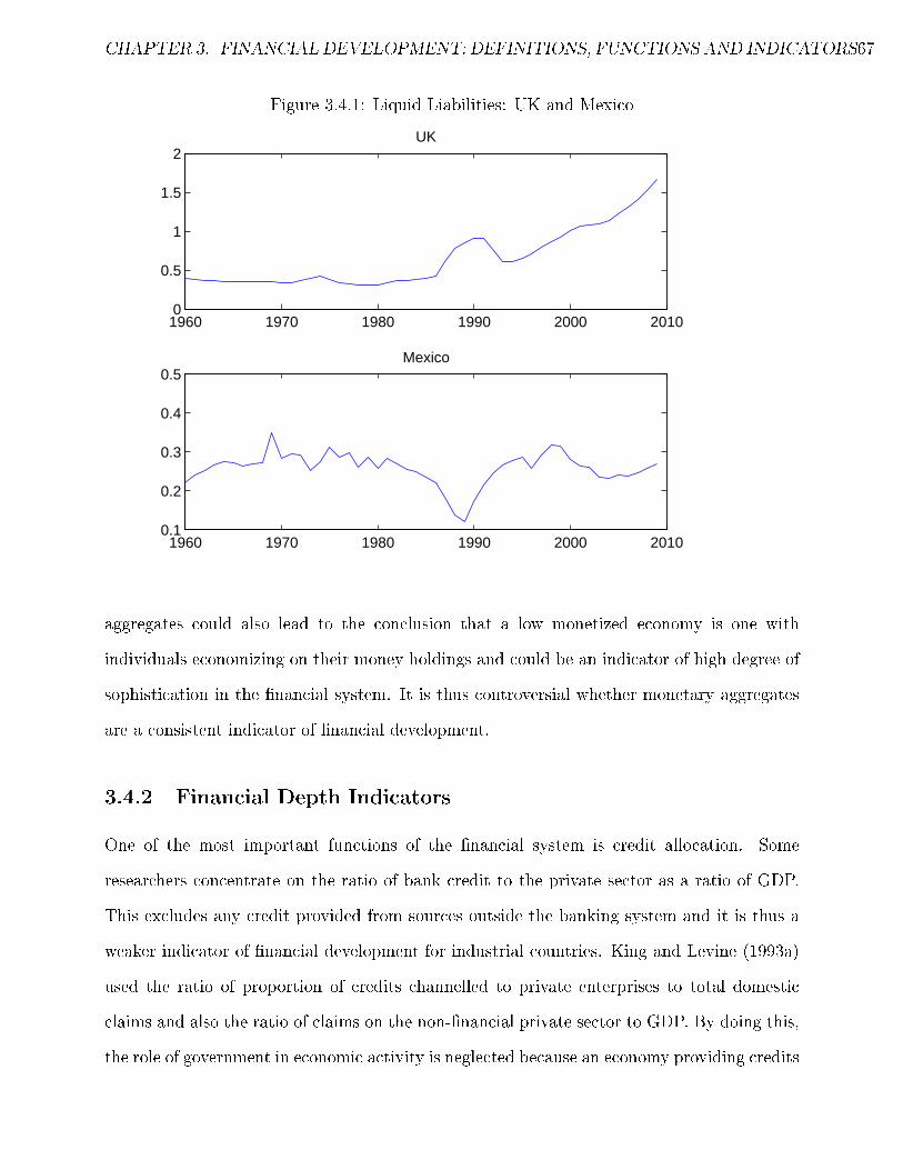
CHAPTER 3. FINANCIAL DEVELOPMENT: DEFINITIONS, FUNCTIONS AND INDICATORS67
Figure 3.4.1: Liquid Liabilities: UK and Mexico
1960 1970 1980 1990 2000 20100
0.5
1
1.5
2UK
1960 1970 1980 1990 2000 20100.1
0.2
0.3
0.4
0.5Mexico
aggregates could also lead to the conclusion that a low monetized economy is one with
individuals economizing on their money holdings and could be an indicator of high degree of
sophistication in the nancial system. It is thus controversial whether monetary aggregates
are a consistent indicator of nancial development.
3.4.2 Financial Depth Indicators
One of the most important functions of the nancial system is credit allocation. Some
researchers concentrate on the ratio of bank credit to the private sector as a ratio of GDP.
This excludes any credit provided from sources outside the banking system and it is thus a
weaker indicator of nancial development for industrial countries. King and Levine (1993a)
used the ratio of proportion of credits channelled to private enterprises to total domestic
claims and also the ratio of claims on the non-nancial private sector to GDP. By doing this,
the role of government in economic activity is neglected because an economy providing credits

CHAPTER 3. FINANCIAL DEVELOPMENT: DEFINITIONS, FUNCTIONS AND INDICATORS68
to the government does not have a strong objective to carry out the functions eciently. A
nancial system providing credit to the government does not eciently full the roles of
evaluating managers or selecting high return risky investments relative to a nancial system
which provides credit to the private sector. However, these indicators are also weak because
they do not fully reect on the level or depth of the nancial services. A study by Leahy,
Schich, Wehinger, Pelgrin, and Thorgeirsson (2001) on OECD countries shows that there
is no statistically signicant relationship between bank credit to GDP ratios and economic
growth rates. Other studies such as Loayza and Ranciere (2004) include developing countries
in their datasets nd a robust relationship between bank credit ratios and growth even though
their nancial systems are not ecient.
An indicator which captures this asset side of the nancial intermediaries is the ratio of
credit to the private sector relative to the GDP (Levine and Zervos, 1998; Levine, Loayza,
and Beck, 1999). The private credit by deposit money banks and other nancial indicators is
dened as claims on the private sector by deposit money banks and other nancial institutions
divided by GDP. It is relatively more informative than any money aggregate variable perhaps
because it excludes the credit to the public sector and thus gives a more precise measure of the
ability of the nancial intermediaries to channel funds from one group to another (De Gregorio
and Guidotti, 1995). It better reects the actual volume of credit channelled into the private
sector. This creates a direct link between the private credit, investment and growth. The
positive relationship between the expansion of credit to the private sector and the economic
growth of a country has been supported by King and Levine (1993a,b). A larger amount
of credit channelled to the private sector in combination with the monitoring functions of
the nancial system, enhances investment in projects that can potentially contribute to the
growth rate of the economy. The German economy is an example of a private credit system
economy where investment nancing is supported mainly by the long term loans expanded
by large and private banks.
However, this indicator excludes the role of security markets as it does not take into
account stock and bond markets. Many of the developing countries have recently experienced

CHAPTER 3. FINANCIAL DEVELOPMENT: DEFINITIONS, FUNCTIONS AND INDICATORS69
Figure 3.4.2: Private Credit to GDP
1960 1965 1970 1975 1980 1985 1990 1995 2000 2005 20100.2
0.4
0.6
0.8
1
1.2
1.4
1.6High Income Countries
1960 1965 1970 1975 1980 1985 1990 1995 2000 2005 20100
0.05
0.1
0.15
0.2
0.25Low Income Countries
1960 1965 1970 1975 1980 1985 1990 1995 2000 2005 20100.1
0.15
0.2
0.25
0.3
0.35
0.4
0.45
0.5Middle Income Countries
a non-bank nancial development with securities markets becoming more important and thus
their role should not be ignored. Just like monetary aggregates, the private credit indicator
also exhibits enormous variation across countries. On average, through the years of 1960
and 2009, countries like Ghana, Haiti and Syria have a private credit of less than 10 per
cent of GDP while others like Switzerland and Japan and United States have more than
85 per cent of GDP. Also, as demonstrated by the late 2000 crisis, an exceptionally high
level of private credit to GDP reects excessive and imprudent lending by the banking sector
(Arcand, Berkes, and Panizza, 2011). If private credit is expanded in an excessive rate and
speed, risks are created at a microeconomic level (misallocation of credit) and macroeconomic
level (leverage which creates susceptibility in adverse shocks).
Financial Systems Deposits to GDP is another widely used indicator of nancial devel-
opment. This is expressed as the ratio of all checking, savings and time deposits in banks
and bank-like nancial institutions to growth per capita. The ratio has a positive correla-
tion with the income level of countries. This size indicator evaluates the size of deposits of
the whole nancial system to with respect to the economy of the country. A greater ratio

CHAPTER 3. FINANCIAL DEVELOPMENT: DEFINITIONS, FUNCTIONS AND INDICATORS70
is considered as a reection to a larger banking system in the sense that more capital can
ow from savers to investors through nancial intermediaries. Other size indicators include
Central Bank Assets to GDP and Money Bank Assets to GDP. These are indicators which
give evidence of the importance of the nancial services performed by these two types of
nancial institutions relative to the size of the economy. Another common indicator is the
ratio of Commercial Bank to Central Bank Assets which primarily measures the extent to
which funds are allocated in a productive manner. This measure is most widely used in
studies of developing countries where the central bank plays a major role in the allocation of
resources (King and Levine, 1993a).
3.4.3 Eciency Indicators and Access Indicators
Financial eciency is more dicult to be captured through indicators. An important aspect
of eciency is the extent to which banks can intermediate society's savings into credit for
the private sector. Asymmetric information, externalities in nancial markets and imperfect
competition (Stiglitz and Weiss, 1992) are signs of inecient investment and allocation of
capital. These features could also lead to bank runs or frauds which impede growth. Eciency
could also be captured through the legal and institutional background of the country.
One indicator capturing eciency is the Bank Credit to Bank Deposits is the claims on
the private sector to deposits in deposit money banks. A low ratio is an indication that
the nancial system of the country does not attract deposits and thus a low share of them
becomes credit for the private sector. The eciency of nancial development shows the
correlation of loans provided by private banks with the loans provided by the central bank
and the percentage of loans given to private non - nancial companies in the number of all
loans. However, taking as evidence from the currently funding instability in world economies,
while a high loan-deposit implies eciency, a `too high' ratio can be a sign that money ows
to the private sector through non-deposit sources. Demirguc-Kunt (2006) emphasizes the net
interest margin and the overhead costs as indicators of eciency. The net interest margin is
a sign competition but also of lower interest rates in developed countries or macroeconomic

CHAPTER 3. FINANCIAL DEVELOPMENT: DEFINITIONS, FUNCTIONS AND INDICATORS71
volatility in emerging economies. High levels of overhead costs as a share of the bank's assets
indicate lower levels of eciency as it is a sign of high bank costs. This leads to another
indicator; the inverse of the spread between banks' lending and deposit interest rates. A
higher wedge between lending and deposit rates illustrates banking ineciency. Usually poor
countries have relatively high net interest margins, overhead costs and lending-deposit rate
gaps.
Access to the nancial system is captured by indicators such as number of ATMs, number
of bank deposits, number of bank branches all relative to total population. Access to nancial
systems allows consumers to smooth consumption over time and stabilises consumer's income
in the case of temporary shocks to wages and income. A commonly used indicator is the
number of loans per capita. It is an indication of the use of credit services. However, the
dierences within income groups make it dicult for this variable to be considered as an
indicator.13 It is generally dicult to capture access to credit by a single or few indicators
because it is aected by all other indications of a sound nancial system as depth, eciency
and composition.
3.4.4 Stock Market Indicators
Although this thesis due to limited data availability concentrates on the depth of the nancial
development, mainly through the banking system, it is worth mentioning few of the indicators
that describe the capital markets. Stock market capitalization to GDP is the most widely
used indicator for the size of the stock market relative to the size of the whole economy.
The activity of stock markets is measured by the stock market total value traded to GDP
which is the total shares traded on the stock market relative to the size of the economy.
Together with the stock market turnover ratio-the ratio of the value of total shares traded
and market capitalization-these are liquidity indicators. Liquidity is considered the most
essential function of the stock market since in economies where long-term commitment of
capital is necessary liquid markets reduce the risk which threatens investment. A large liquid
13In Poland there are 770 bank loans per 1000 people but only 94 in Venezuela (Demirguc-Kunt, 2006).

CHAPTER 3. FINANCIAL DEVELOPMENT: DEFINITIONS, FUNCTIONS AND INDICATORS72
market allows savers to buy equity and sell it quickly whenever they are found in need for
their savings or in desire to alter their portfolios. Opening up a liquid trade and acting
as a price determining mechanism for nancial instruments, stock market spreads the risk
between investors and capital raisers. This activity increases investment and reduces the
cost of capital. This in turn ameliorates the allocation of capital, improves investment and
enhances growth (Levine, 1997). A country with organised and liquid market is able to
attract a FDI and portfolio investment leading to an increase in capital inow and funds in
the country to nance current account decits. The liquidity oered is an encouragement
for domestic investors to transfer their surpluses into long term capital and enjoy economies
of scale. Merton (1987) declares that as markets become larger and more liquid, it becomes
easier to acquire information and thus the incentive to invest increases since any private
information can be translated into money. On the other hand, very liquid markets can also
lead to investor myopia. The fact that they can sell an asset quickly when they are displeased
means less commitment and incentive for corporate control or monitoring rms' performance
and this can impede economic growth (Levine, 1997). The connection of these indicators
with growth is that, high income countries tend to have relatively larger and more liquid
stock exchanges.
3.5 Conclusions
This chapter started with a clear denition of nancial development. It provided a detailed
description of the functions of nancial institutions through the building of a simple AK
model. The reader is introduced to the indicators of nancial development used by many
researchers over the years and gives justies the use of private credit to GDP ratio as the
main indicator for this thesis by emphasising the disadvantages of other indicators. This
chapter separated the indicators according to size, access and depth to familiarise the reader
with the concept of nancial development. The main conclusion is that nancial institutions
are given the role of an intermediary between the saver and the lender and the functions of a
nancial system aid in materialising long term projects which have an impact on productivity

CHAPTER 3. FINANCIAL DEVELOPMENT: DEFINITIONS, FUNCTIONS AND INDICATORS73
and thus growth. It is this impact that subsequent chapters will try to test and analyse.

Chapter 4
Financial Development and Growth: A
Survey on the Empirics
4.1 Introduction
Theory suggests that eective nancial markets and institutions enhance economic growth
and the welfare of a country. Some researchers claim that countries which are relatively less
nancially developed are also relatively less economically developed. Others give no role of
the nancial system in the real sector of the economy. Either way, after the pioneering work of
Goldsmith (1969), researchers attempt to prove any kind of relationship between the nancial
and the real sector.1 Albeit a score of empirical studies investigating the relationship between
nancial development and economic growth, the result is ambiguous. The main empirical
research focuses on three types of regressions in order to establish a relationship between
nancial development and economic growth; cross country with or without panel techniques,
time series, and microeconomic-based techniques. The channels of transmission in explaining
the nance-growth relationship dier across studies but most of them provide a positive link
between nancial development and growth.2 Since relationship never implies causality, many
studies also attempt to nd a causal link between nance and growth using co-integration
1See Levine (1997, 2005) for extensive literature on the theory.2Appendix C provides a review of the most cited papers in the literature of nance and economic growth.
74

CHAPTER 4. FINANCIAL DEVELOPMENTANDGROWTH: A SURVEYON THE EMPIRICS 75
techniques and Granger causality tests. Advances in computational capacity and increases in
the availability of country and time data drove researchers away from cross country techniques
towards Panel Data techniques to explore the relationship between nancial and real sector.
Section 4.2 provides a review of the empirical evidence of some cross country, time series and
panel data studies. Section 4.3 gives a small review of the studies focusing on causality and
on one country cases. Section 4.4 describes the econometric caveats of all three approaches.
The conclusions are in Section 4.5.
4.2 Empirical Approach to the Finance-Growth Nexus
4.2.1 Cross Country Studies
The application of cross country techniques involves aggregating economic growth over long
periods such as a decade or more and examining the relationship between measures of nan-
cial development and long run economic growth.3 Goldsmith (1969) was the rst to show
the presence of a positive correlation between the size of the nancial system and long-run
economic growth. The size of nancial development was captured by the ratio of the value
of intermediary assets to GNP and economic growth based on data for 35 countries over the
period of 1860-1963. He argued that the positive relationship was driven by nancial inter-
mediation improving the eciency rather than the volume of investment. However, three
main problems arise in this study. Firstly, although the period of study is long, the sample
size is small. Secondly, no work is provided on the direction of causality. Lastly, no other
factor that might inuence growth is controlled for in his work. Although the problems of
Goldsmith (1969) were evident, empirical studies only emerged in the early 1990s. King and
Levine (1993a,b) solve the sample problem by working on 80 countries on a 30-year horizon
(1960-1989). King and Levine (1993b) study controls for a number of potential determinants
of economic growth such as initial income, educational attainment, ination and government
3In principle the average inuence of the determinants of economic growth is estimate. A number of studiesthat have dealt with this issue are,Gelb, 1989, WorldBank, 1989, Roubini and Sala-i Martin, 1992, Fry, 1997and King and Levine, 1993a. Durlauf, Johnson, and Temple (2005) provide a review on the econometrics ofthe cross-country growth literature.

CHAPTER 4. FINANCIAL DEVELOPMENTANDGROWTH: A SURVEYON THE EMPIRICS 76
spending. Their study considers productivity growth and capital accumulation as the chan-
nels through which nance could aect growth and thus examine the association of nancial
development indicators within these channels. Their ndings support a positive and sig-
nicant relationship between several nancial development indicators and economic growth.
Their paper also examines whether the size of the nancial system in 1960 can predict the
rate of any of the dependent variables over the next 30 years. The results convey that indeed,
the vector of the nancial indicators is a good predictor of the subsequent rates of economic
growth, capital accumulation and productivity growth. De Gregorio and Guidotti (1995)
use a growth regression4 to examine the relationship between long run economic growth and
nancial development using a dataset of 95 countries between 1960 and 1985. The bank
credit to non-nancial sector is used as the explanatory variable and the ndings support
a positive relationship between intermediation and real growth and more specically that
nancial development is related to improved growth performance. These studies concentrate
only on the banking system by using size indicators of nancial development. They fail to
take into account other measures which could directly measure the ability of the nancial sys-
tem To overcome this limitation, some studies attempt to examine the role of stock markets
in promoting economic growth. Atje and Jovanovic (1993) show that stock markets have
both positive level and growth eects on economic activity. According toDemirgüç-Kunt
and Levine (2004), and conrmed by Demirgüç-Kunt and Maksimovic (1998) and Levine
and Zervos (1998)) these studies are important for governments' to set reforming priorities
in the dierent segments of the nancial system. Levine and Zervos (1998) use data from
1976 to 1994 to examine whether banking or stock market contribute more in the growth
accounting equation. They nd a positive and signicant relationship between stock market
(measured by turnover or value traded to GDP) and bank development with GDP per capital
growth. More specically, they show that one standard deviation in stock market liquidity
and banking sector explains a dierence of 0.8 and 0.7 respectively in annual GDP per capita
growth. These results suggest that whether the type of the nancial system is market based
4The growth regression is presented in Section 4.4.

CHAPTER 4. FINANCIAL DEVELOPMENTANDGROWTH: A SURVEYON THE EMPIRICS 77
or bank based is of secondary importance in the growth process.5 Other empirical work such
as Beck and Levine (2002) compares the two and support the bank based idea. However,
the evidence from Levine and Zervos (1998) content that the important feature for growth is
the existence of liquid and ecient nancial intermediaries, regardless of whether there are
equity markets or banks. Moreover, their empirical work becomes important for policy as it
conveys that equity markets and banks are complements rather than substitutes and thus in
markers such as the European one, market based economies and bank based economies can
coexist and both can promote growth. Their results coincide with those of Levine (1991)
and Bencivenga, D., and M. (1995). The same conclusions are drawn from the studies of
Levine, Loayza, and Beck (1999) and Beck, Levine, and Loayza (2000) which nd a signi-
cant impact of nancial intermediation indicators on the real GDP growth and productivity.
They however nd an ambiguous eect on physical capital growth and saving. In contrast
to these results Harris (1997) shows little support on the view that stock markets help to
explain growth rates especially in the developing countries.
More specic research comes from La-Porta, Lopez-De-Silanes, and Shleifer (2002) where
the state ownership of the banking sector is the proxy for nancial development. The cross
country regression reveals that the ownership and control of the banks in the 1970s con-
tributed negatively to the growth process. They control for institutional quality controls
and also disentangle the eects of state ownership on investment and productivity and show
that although investment is not signicantly aected, productivity is largely aected. The
conclusion of their research is that public intervention in the credit markets deters resource
allocation. This is in contrast to other research such as Sapienza (2004) and Papaioannou
(2005) which give evidence for supporting public choice theories.
Aghion, Howitt, and Mayer-Foulkes (2004) test the eect of nancial development on
convergence. Adding the nancial sector in a Schumpeterian model of the 19th century imply
that all countries above some threshold level of nancial development should converge in
5Demirguc-Kunt and Levine (1999) analyse cross section growth regression and conclude that countriesbecome more market based as their income increases. Chakraborty and Ray (2006) provide a theoreticalmodel and nd that neither system is unambiguously better for growth, but a bank-based system relativelyoutperforms a market-based one along other dimensions.

CHAPTER 4. FINANCIAL DEVELOPMENTANDGROWTH: A SURVEYON THE EMPIRICS 78
growth rate, and that nancial development has a positive but gradually diminishing eect on
steady-state GDP. The authors test these implications by estimating a cross-country growth
regression by augmenting it by an interaction term between nancial development and the
country's initial relative output relative to the US GDP. The countries with higher nancial
development have a higher probability of converging to the U.S growth rates. They conclude
however that the direct eect of nancial development is not signicantly dierent from zero.6
La-Porta, de Silane, Shleifer, and Vishny (1997) consider the dierences in countries' legal
origins an exogenous factor for the development of the countries' nancial development. It
is exogenous because most of the countries obtain their legal systems through colonization
or occupation. They thus develop the legal origins hypothesis where legal systems aect
nancial development and thus economic activity. Whether a country enforces laws from the
British, French, German or Scandinavian background laws, its growth process depends on
these through the impact of law on the nancial systems. The empirical work that followed
has emphasised that the legal system signies an essential determinant of economic growth,
especially in relation to nancial development. The idea is that any nancial instrument
needs a legal system to support it. For example, the legal system makes it harder for a
debtor to default on its debt obligation. It acts as a protection line between the rights of
the borrowers and the lenders. The legal origins variable is captured through Instrumental
Variables (IV) such as the legal rights of creditors, the soundness of contract enforcement and
the level of corporate accounting standards. The authors try to distinguish how important is
the legal systems for the rms in need of external nance. The results imply that countries
with better legal protections have higher and broader capital markets and more external
nance. The studies that followed such as Levine (1998), Demirgüç-Kunt and Maksimovic
(1998) and Levine (1999) also show that the nance-growth nexus is statistically signicant.7
Some other cross country studies such as Levine and Renelt (1992) and Sala-i Martin
6Aghion and Howitt, 2006give a review on the Schumpeterian growth models of technological innovationand attempt to identify specic channels through which nance aects economic growth in cross countryregressions (see also Howitt, 2000)
7The main problem of using the IV approach is that legal origin may aect economic growth through athird channel, for example through regulation. Acemoglu and Johnson, 2003 nd that in such cases, their IVestimates are biased upwards and interpreted as upper bounds of the true eect of nancial development.

CHAPTER 4. FINANCIAL DEVELOPMENTANDGROWTH: A SURVEYON THE EMPIRICS 79
(1997) perform a regression where a range of non-nancial variables explain real growth to
some extend while nancial variables are found to be ineective. Odedokun (1996) examines
81 countries and concludes that money aggregates have a negative eect on marginal produc-
tivity. Harris (1997) argues that the eect of stock market activity in less developed countries
relative to developed countries is rather weak. Results from studies such as those of Shleifer
and Vishny (1986) and Shleifer and Summers (1988) support the negative implications of
stock market liquidity. Also Ram (1999) makes a use of annual data for 95 countries over
1960-89 and shows that the correlation between nancial development and economic growth
is negligible or negative even if the regression is applied to each individual country or on
groups of countries according to their income levels.
Table 3.1 displays a number of cross country studies stated by their results. Most of the
studies conclude on a positive relationship between dierent indicators of nancial develop-
ment and growth.
4.2.2 Time-Series Studies
Following Arestis and Demetriades (1997), time-series explore the nance-growth relationship
mainly through the application of Granger causality tests in a vector autoregression system
of equations (VAR). Most of the cross country studies take for granted that the link between
nancial and real sector runs from nance to real economy. On the contrary, time series
studies give priority to the issue of causality. Time series results rarely give a clear directional
causality pattern between nance and the real sector. The rst time series study is that of
Gupta (1984) working on 14 developing countries. Using monetary indicators as well as
private credit to measure nancial development and industrial production as an index of
economic development, his study supports that causality runs from nancial development to
growth. However, his results are unreliable considering that the industrial production is only
a small portion of the total output in particular for most of the developing countries.
Patrick (1966) supports the hypothesis that the direction of causality alters over the
development process. At initial levels of economic development a supply-leading pattern is

CHAPTER 4. FINANCIAL DEVELOPMENTANDGROWTH: A SURVEYON THE EMPIRICS 80
observed where the creation of nancial institutions is responsible for higher growth through
a reallocation of resources from traditional to modern sectors. At later stages, the demand-
following hypothesis develops where the need for nancial services coming from higher growth
leads to an expansion of the nancial system. Jung (1986) applies Granger causality tests
for 56 countries for the period 1950 to 1981 and provides support for the supply leading
hypothesis. Hansson and Jonung (1997) examine the case of Sweden over 1834 and 1991
and argue that a bi-directional causality is observed between bank credit and real output for
1834 to 1991 whilst a supply-leading relationship occurs for 1890-1934. Neusser and Kugler
(1998) use the nancial sector GDP as a proxy for nancial development and manufacturing
GDP as an indicator of economic growth and apply causality tests to nd results consistent
with the supply leading view and conclude that nance is important for growth. They also
apply cointegration and causality tests on 13 OECD countries between 1960 and 1994 and
nd that the causal link between nance and the real sector is weak especially for the smaller
countries. They however establish a feedback from manufacturing GDP to nancial services
without making inferences on the direction of causality. Similar studies and conclusions are
obtained by Demetriades and Luintel (1996); Greenwood and Smith (1997); Luintel and Khan
(1999); Rousseau and Vuthipadadorn (2005); Xu (2000) The latter applies an examination
on 41 countries between 1960 and 1993 and rejects the hypothesis that nancial development
merely follows economic growth and has a negligible eect on it.
Cross country studies usually treat developed and developing countries as belonging to the
same category. Demetriades and Hussein (1996), as well as Arestis and Demetriades (1997),
separate these two groups of countries and examine them separately to prove the variability
across countries even if the same estimation techniques are used. They content that dierent
countries have dierent institutional systems and some of these systems are relatively more
signicant for growth. They conclude that even if countries have the same level of nancial
development, dierent nancial sector policies and institutions alters the impact of nance
on growth. Demetriades and Hussein (1996) reveal evidence of bi-directionality and reverse
causation when applying causality tests on 16 developing countries. Claiming that nance

CHAPTER 4. FINANCIAL DEVELOPMENTANDGROWTH: A SURVEYON THE EMPIRICS 81
leads growth it is thus dangerous for policies and institutions in the developing countries.
Rousseau and Wachtel (1998) examine the period of 1871-1929 USA, Canada, Sweden, Nor-
way and UK over a period of 1871-1929. The large time span allows for testing long term
causal patterns like those described by Patrick (1966) and Gerschenkron (1962). Their study
claims that the nance-growth nexus is driven by nancial intermediation variables which
aect the growth process.
In a more recent empirical work examining the case of Malaysia, Ang and McKibbin
(2007) use a multivariate cointegration approach analysis to index nancial development
in order to overcome issues of over-parameterization. A number of causality tests used in
their study concludes that growth is causing nancial development in the long run. However,
Caporale, Howells, and Soliman (2005) examining the same country while using stock market
data concludes that the stock market development enhances economic growth through a rise
in the eciency of investment which feeds back to productivity. These results highlight
the debate of bank based versus market based economies in promoting growth. Arestis,
Demetriades, and Luintel (2001) argue in favour of banks, that the role of stock markets
has been over-emphasized by cross-country studies. They even nd a negative eect of stock
markets in ve of the developed countries examined. Against this view, Thangavelu and
Ang (2004) using Australia as the case study show that economic development increases the
demand for banking services and causes an enhancement of the nancial sector. There are
also cases of neither demand-following nor supply-leading hypothesis. Chang (2002) uses
multivariate VAR models for Mainland China to test both of these hypotheses. Based on
multivariate error correction models (ECM), Granger causality implies no dependence of
nance on growth or vice versa.
Time series studies give mixed conclusions on the issue of causality. Table 3.2 outlines
some of the most inuential time series studies. What is noticed however is that supply
leading patterns tend to occur somewhat more frequently than demand-following.

CHAPTER 4. FINANCIAL DEVELOPMENTANDGROWTH: A SURVEYON THE EMPIRICS 82
4.2.3 Panel Studies
Dynamic panel estimation techniques have been used in order to eliminate the problems of
cross country studies. Panel techniques allow for nancial development and growth deter-
minants that are time-invariant unobserved country characteristics to be controlled.8 Fixed-
eect panel techniques are subject to less endogeneity problems. Heterogeneous country
eects are allowed and thus nancial development has dierential eects across countries.
Among many others, the empirical studies of Levine, Loayza, and Beck (1999), Beck, Levine,
and Loayza (2000), Benhabib and Spiegel, 2000, Rousseau and Wachtel (2000), Beck and
Levine (2004) and Rioja and Valev (2004) convey a positive relationship between indicators
of nancial development and growth. Gertler and Rose (1991) develop one of the rst panel
studies on the nance-growth nexus and nd that a one percentage point rise in per capita
income is associated with a one and a half percentage point increase in private domestic
credit and the relation is very robust. Berthélemy and Varoudakis (1997) apply a xed eect
model for 82 countries. Although they establish a negative relationship between nance and
growth, they claim that under poverty traps, nancial systems cannot eciently full their
functions and that the impact of a poor nancial system is that it holds the economy stable
at a low equilibrium.
Loayza and Ranciere (2004), use a dynamic panel pooled mean group estimator employed
by Pesaran and Smith (1995) to internalize parameter heterogeneity and conclude that there
is a positive signicant relationship between nance and growth in the long run but not in
the short run. This nding is supported by the idea that too much nance in the sense
of fast expanding credit can lead to nancial crisis and thus impede economic growth. Ar-
cand, Berkes, and Panizza (2011) using cross country and panel techniques convey the same
conclusion. Levine, Loayza, and Beck (1999) use a GMM estimator developed by Arellano
and Bond (1991) for panel data. They nd a positive relationship between the exogenous
nancial development factor and economic growth, capital accumulation and productivity
growth. Calderón and Liu (2002) use the Geweke decomposition test on 109 developed and
8See Bond, Hoeer, and Temple, 2001 for a discussion of the GMM dynamic panel techniques used inmost of the empirical growth models with a panel set of data.

CHAPTER 4. FINANCIAL DEVELOPMENTANDGROWTH: A SURVEYON THE EMPIRICS 83
developing countries conveying a bi-directional causality. Christopoulos and Tsionas (2004)
use panel unit roots and panel cointegration techniques and conclude that causality runs
from nancial development to economic growth but they nd no feedback relationship.
Micro level studies also employ panel techniques. Such studies attempt to lessen limita-
tions such as omitted variable, reverse causality and multicollinearity. The micro approach
helps to increase understanding of the theoretical mechanisms behind nance and growth.
Rajan and Zingales (1998) work on a cross-country cross-industry approach and content that
a better developed nancial system help reduce market frictions which otherwise create a
wedge between the cost of external and internal nance. This helps the industries which are
highly dependent on external nance to expand proportionately more than the rms which
are not as dependent on external nance. In general, the rms using external nance based
in highly developed countries tend to prosper more compare with other rms. They use
industry level data (36 manufacturing industries) and 41 countries and propose a two-step
approach. They rst construct a measure for external nance and then test whether sec-
tors highly dependent on external nance tend to grow faster. The important innovation
of this paper is the introduction of both country and industry xed-eects. Studies that
followed conrm the strong positive eect of nancial development with industry growth and
hence economic growth (Demirguc-Kunt and Maksimovic, 2002; Claessens and Laeven, 2004;
Braun, 2003; Bertrand, Schoar, and Thesmar, 2007; Guiso, Jappelli, Padula, and Pagano,
2004; Allen, Qian, and Qian, 2002).9
4.3 A note on Causality and Country Specic Studies
The ambiguity arising from the conclusions of these studies is explained according to Al-
Yousif (2002) by the fact that most of the studies focus on the correlation between nance
and growth and this does not demonstrate or imply any causality direction. The issue of
causality direction between nancial development and the real sector is a central aspect
9Ciccone and Papaioannou, 2005 apply a micro approach to assess the impact of human capital on growth.Others use this method to explore the impact of product market regulation on rm entry (Perotti and Volpin,2004; Fisman and Sarria-Allende, 2004)

CHAPTER 4. FINANCIAL DEVELOPMENTANDGROWTH: A SURVEYON THE EMPIRICS 84
among researchers. Evidence on causality can inuence policy reforms and their degree of
importance in enhancing nancial intermediary development. Imperative statements such as
banks were the happiest engines that ever were invented by Hamilton (1781) and banks
harm the morality, tranquillity, and even wealth by President John Adams (1819) ought to
be made only when causality has been established. It is possible that nancial development
is merely the leading indicator of economic growth instead of a causal indicator.
Studies concentrating on causality however, also lead to ambiguous results most probably
because of simultaneity, omitted variables, nonstationarity of variables, insucient sample
size and unobserved country specic eect. To solve the problem of small sample size, Holtz-
Eakin, Newey, and Rosen (1988) use a panel vector autoregression model (VAR) with a
large cross country sample under a small period of time. In 1984, Gupta used quarterly
data of industrial output of 14 developing countries to measure economic development and
reported a direction of causality from nancial development to economic growth. Rousseau
and Wachtel (2000) use Arrelano and Bond procedure of testing causality in a VAR model
providing evidence of causality from nance to growth. Levine, Loayza, and Beck (1999)
use a GMM dynamic panel estimator and instrumental variables capturing cross country
characteristics to address the issues of simultaneity and unobserved country specic eect.
Calderón and Liu (2002) apply tests of linear dependence and Geweke test to establish the
direction of causality in a panel data set of 109 countries. They nd a feedback eect which
implies that nancial development promotes economic growth and at the same time economic
growth is a catalyst for nancial development. They also nd that the degree of causality
from nance to growth is bigger in the developing than in the developed countries. Moreover,
causality tests show that nancial development causes total factor productivity growth which
is relatively greater in developing countries.
Integration and cointegration properties of the data are introduced in Christopoulos and
Tsionas (2004) work which also concludes in a unidirectional causality from nance to growth.
They test the long run relationship between the nancial sector and the real sector by ap-
plying unit root test, panel cointegration analysis, cointegration test and dynamic panel

CHAPTER 4. FINANCIAL DEVELOPMENTANDGROWTH: A SURVEYON THE EMPIRICS 85
data estimation for a panel vector error correction model (VECM). Their ndings suggest a
unitary equilibrium relation between nancial deepening and economic growth as well as a
support for the nance-led hypothesis in the developing countries of their sample. Pesaran,
Pick, and Timmermann (2011) propose a dierent than the traditional Engel and Granger
approach to causality which is superior in that it is applied even if the regressors are not
purely stationary or integrated. It is also statistically more ecient in the case of small sam-
ples. In 1995, Toda and Yamamoto (1995) estimated a VAR which guarantees the asymptotic
distribution of the Wald statistic through the robustness of the integration and cointegra-
tion properties of the process. Esso (2010) use both of these techniques and conclude that
for some developing countries GDP per capita signicantly causes nancial development in
Cape (`demand-following' view) as conrmed by Demetriades and Hussein (1996). In some
other countries however nancial development `leads' economic growth and agrees with the
`nance - led' growth hypothesis. Hurlin and Venet. (2001) however, nd that causal rela-
tionship from growth to nance, occurs in developed than in developing countries. Apergis,
Filippidis, and Economidou (2007) examine whether a long-run relationship between nance
and growth exists using panel integration and cointegration tests. Their results support a
bi-directional causality between nancial deepening and growth, which remains robust to
various specication of the sample.
A major constraint in establishing causality empirically is that time series for developing
countries is not widely available. Cross country studies built aim to break this constraint but
as Ahmed (1998) argues, the issue of causality cannot be addressed in such a framework since
each country has its policies and its own nancial institutions (Demetriades and Andrianova,
2004; Kirkpatrick, 2005). Since each country has its own characteristics such as social capital,
law and regulation, researchers move towards examining the long run relationship between
nance and growth in country-cases. Country-specic studies establish a relationship be-
tween the local policy frameworks, nancial development and growth within a special case
and attempt to overcome the diculties arising from eorts to disentangle country-specic
characteristics. For example the U.S removed regulatory restrictions on branching and bank

CHAPTER 4. FINANCIAL DEVELOPMENTANDGROWTH: A SURVEYON THE EMPIRICS 86
ownership. Jayaratne and Strahan (1996) relate the impact of such changes to growth and
conclude that state banking deregulation is associated with an increase in GDP per capita.
Individual country studies become essential for policy in the EU since it gives evidence on
how the banking and nancial integration aects productivity and hence the growth rate.
Such evidence are given by Guiso, Sapienza, and Zingales (2004) who investigate the eects
of rm access to nance and how it aects the growth of dierent Italian regions. Financial
development turns out to be a fundamental characteristic in the growth process. Ang and
McKibbin (2007) use data available from Malaysia use multivariate cointegration and tests
of causality and argue that output growth enhances nancial development in the long-run.
They control for multicollinearity and upward bias in the estimators by using nancial in-
dicators constructing nancial development index. Thangavelu and Ang (2004), nd that
economic growth Granger causes nancial development in Australia through an eect on the
banking sector. Rao and Tamazian (2008) use Indian data to reject the view that nance
follows where enterprise leads. Using panel data in China, Aziz and Duenwald (2001) cannot
support the hypothesis that nancial development boosts economic development. Kilimani
(2007) provides evidence on the link and causality between the nancial and the real sec-
tor in Uganda and contend that causality runs from nancial development to growth when
M2/GDP is used as a proxy indicator. Although country case studies are important for ex-
amining the relationship between nance and growth at a national level, they cannot be used
for general inferences on this relationship. The results obtained from one country cannot
constitute as a reference for policy formulation in other countries.
4.4 Limitations of the Empirical Research
Most of the empirical work that follows after the work of Goldsmith (1969) uses a Barro-type
regression summarised in equation 4.4.1:
gi,t = ∆ln (yi,t) = α + βifi,t + γiCi,t + µi + εi,t (4.4.1)

CHAPTER 4. FINANCIAL DEVELOPMENTANDGROWTH: A SURVEYON THE EMPIRICS 87
where ln (y) is the log of real GDP per capita or any other form of welfare available,
g is the growth rate of y, f is an indicator of nancial development, C is a conditioning
information set,µ is a country specic element of the error term without necessarily being
distributed with a mean of zero, ε is an error term with a mean of zero, i is the country,
industry, rm or household according to the type of study and t is the time period. The focus
falls on parameter βi as its signicance and sign are under debate. This parameter can be
biased and results can be inconsistent because of measurement error, lack of appropriate data,
reverse causation and omitted variable bias. For many years, the f vector included variables
capturing the size, eciency and activity of banks and thus included monetary aggregates or
private credit to GDP. In later years especially after 2000, this vector is expanded to include
the size, liquidity and eciency of the stock markets especially for the developed countries
since the data for the developing ones is scarce. Micro-based data and non-bank nancial
institutions data is also used in recent research.
4.4.1 Cross country growth equation
The common cross country equation is of the form
gi = ∆ln (yi) = α + βfi + γCi + δln (yi,t−1) + εi (4.4.2)
This regression equation only has cross country but not time series dimension. The ini-
tial level of income, ln (yi,t−1) enters to control for convergence predicted by the neoclassical
Solow-Swan models (i.e. the further away a country is from its steady state, its growth rate
will be higher). Benhabib and Spiegel (2000) replace this term by the physical capital ac-
cumulation ∆ln(Ki). The growth rates and the explanatory variables are measured as an
average over the sample period or as an initial value. Cross country studies examine the
sign and signicance of parameter β as evidence for a partial correlation between nance
and growth. The conditional set of variables includes initial levels of human or physical cap-
ital, institutional quality, geography, government policy variables to allow for cross country
dierences in productivity and testing for an independent partial correlation of nance with

CHAPTER 4. FINANCIAL DEVELOPMENTANDGROWTH: A SURVEYON THE EMPIRICS 88
growth. If β takes a positive and signicant value is a sign of a positive partial correlation be-
tween nancial variables and growth. The pioneers of empirical work on nance and growth
King and Levine (1993a) as well as Levine and Zervos (1998) used regression 4.4.2 using bank
variables and stock market variables respectively. Both of these papers nd a positive link
between measures of nancial development and growth. Although the results are statistically
and economically signicant OLS estimates can be aected by an unobserved country spe-
cic eect, µi as in equation 4.4.1. For example Aghion, Howitt, and Mayer-Foulkes (2004)
content that countries who have room from improvement and are thus away from the tech-
nological frontier are relatively more aected by the eciency in the nancial intermediaries.
Moreover, countries with higher human capital or greater openness to trade tend to nd
nancial development more useful. Thus, the eect of nancial development may not be
homogeneous across countries. Such an eect breaks down the orthogonality conditions
E(C′
iεi) = 0 (4.4.3)
E(γ′
iεi) = 0 (4.4.4)
E(f′
i εi) = 0 (4.4.5)
and leads to a positive correlation of the lagged dependent variable with the error term
hence
E[γ′
i,t−1(µi + εi)] 6= 0 (4.4.6)
Omitted variable bias is very likely in such regressions if other explanatory variables are
also correlated with µ or if some explanatory variables are ignored from the equation and
thus
E[C′
i(µi + εi)] 6= 0 (4.4.7)

CHAPTER 4. FINANCIAL DEVELOPMENTANDGROWTH: A SURVEYON THE EMPIRICS 89
It is impossible to control all the likable factors that may prosper economic growth. There
is data for more than a hundred countries and a large set of C that can foster growth. The
eect of omitting variables can be tested by adding more variables in an existing equation.
Garretsen et al. (2004) argue that as legal and social capital factors are added in the re-
gression, the positive β observed by Levine and Zervos (1998) no longer holds. Moreover,
as Rioja and Valev (2004) nd, grouping countries according to their nancial development
levels gives a dierent impact of nance on growth. The static assumption in these broad
pure cross country regressions means that the model is made into a one-period framework.
Inferences about the long run are thus unveriable since economic growth is a long term
phenomenon and a long time series data is a sucient and necessary condition for inferences
and analysis of the nance-growth link. These are factors that make cross country studies
susceptible to the sample of countries, the control variables used, the time span used and the
econometric application.
Multicollinearity arises among the regressors and is thus hard to disentangle the eect
of the dierent independent variables on economic growth. One can conclude that well-
developed countries have well-developed nancial systems. However, they also have well-
developed education systems, political stability, high institutional quality etc. The inter-
correlation between the regressors has led to only a few variables being considered as sig-
nicant determinants of economic growth (Levine and Renelt, 1992; Sala-i Martin, 1997;
Sala-I-Martin, Doppelhofer, and Miller, 2004). Measurement error is another issue with
pure cross country studies. There is a possibility that nancial development indicators are
inaccurate such that
(fi) = fi + ui (4.4.8)
where fi is the true level and f is the measured level of nancial development. If,
E(ε′
iui) 6= 0 (4.4.9)

CHAPTER 4. FINANCIAL DEVELOPMENTANDGROWTH: A SURVEYON THE EMPIRICS 90
then the equation 4.4.2 suers from attenuation bias which implies that the estimates are
conservative. Measurement errors can occur due to data problems. There is no grounded
theory for establishing proxies of nancial development. Usually nancial indicators are con-
structed taking into consideration the channels through which nance aects growth. How-
ever, measurement error may lead to upward bias of the estimated nancial development
parameter especially if other variables from the conditioning set are measured with error.
This is because is likely for the coecient on nancial development to capture part of the
eect of these miss-specied variables.10 There is also a lack of high quality data. This may
prevent researchers from gathering information on historical nancial environment of indi-
vidual countries. Thus a cross country regression can say little about any policy implications
ought to be pursued.
Reverse causation is another limitation of pure cross country studies. Most of the cross
country studies take for granted the nance led view and expand models based on this
assumption. However, nancial development can cause economic growth but also be caused
by economic growth. The relationship between the nancial sector and the real sector may
be due to economic growth leading to an expansion of nancial services. Demetriades and
Luintel (1996, 2001) specify an equation where the nancial development vector becomes the
dependent vector and nd a positive impact of economic growth on f. Since this potential
endogeneity is not controlled for in such simple equations, the estimators are likely to be
biased and inconsistent. It is possible that nancial development indicators such as market
capitalization increase when future growth is expected and thus,
fi = θyi,t−1 + vi (4.4.10)
and also,
E(ε′
ivi) 6= 0 (4.4.11)
10As an example consider a regression equation with human capital and nancial development. If oneassumes that human capital is is measured with some error but nancial development is not, then thecoecient of nancial development will capture part of the human capital proxy which has not been specied.More details are given by Mankiw (1995) and Krueger and Lindahl (2000).

CHAPTER 4. FINANCIAL DEVELOPMENTANDGROWTH: A SURVEYON THE EMPIRICS 91
which violates the orthogonality condition. Reverse causality should not be ignored be-
cause as it may may suggest some underlying structural problems such as political inter-
ference in the nancial system, corruption, political uncertainty, economic uncertainty such
as ination etc. An approach that gives relatively less biased results is the use of a set of
simultaneous equations so that a specication for the nancial development equation is clear.
Researchers search for instrumental variables to extract the exogenous component of
nancial development. Instrumental variables need to be correlated with nancial interme-
diaries' indicators as to explain cross country dierences in nancial development but also
be uncorrelated with economic growth besides their link with nancial development.
Remedies to endogeneity and other biases include instrumental variables in the regression
equation. These are instruments used to disentangle the eect of the endogenous variable
that is not related to any of the biases. It is a way to control for the possibility that
nancial development and growth are both caused by other factors. The most common
instrumental variable is the legal origins of the country as explained above. The research of
law and nance identies variables which explain nancial structure but not economic growth.
Other instruments include proxies for geographic conditions, (Sokolo and Engerman (2000))
religion and culture (Stulz and Williamson, 2003). Including instrumental variables changes
the simple regression equation into the following set of equations
gi = α1 + β1fi + γ1Ci + δ1ln (yi,t−1) + εi (4.4.12)
fi = α2 + β2Zi + γ2Ci + δ2ln (yi,t−1) + χi (4.4.13)
(fi) = fi + ui (4.4.14)
where C and Z are the included and the instrumental variables respectively. Vector Z
allows the identication of that part of fi which is uncorrelated with εi and thus

CHAPTER 4. FINANCIAL DEVELOPMENTANDGROWTH: A SURVEYON THE EMPIRICS 92
E(Z′
iεi) = 0 (4.4.15)
E(Z′
iui) = 0 (4.4.16)
Equation 4.4.12 is estimated by two stage least squares (TSLS) and it is considered to
solve for omitted variable bias, measurement error and reverse causality. TSLS estimator can
also be obtained by GMM. However, Ahmed (1998) and Ericsson, Irons, and Tryon (2000)
claim that the use of instrumental variables as a solution to endogeneity is inecient because
when the data is averaged over a long period of time the growth dynamics are diluted and
the regressions can lead to spurious relationships. The original data may not be contempo-
raneously correlated unlike the time-averaged data. Testing the conditions 4.4.15 and 4.4.16
requires the Sargan test (Sargan, 1958). Nevertheless, testing for overidentifying restrictions
is relatively weak as it i) needs a greater number of instrumental variables compared to ex-
ogenous variables and ii) tends to reject the validity of instruments if the sample is small
(Murray, 2006). The problem of causality also remains as instrumental variables in cross-
country regressions focus on the endogeneity of nancial development and thus all of the
other control variables are treated as exogenous. Setting a priori a belief on causality based
on theory does not help in determining the causal relationship of the variables. Moreover,
instrumental variables approach ignores the independent and simultaneous eect of equity
markets. Lastly, if the excluded exogenous variables are weak, the IV results are biased
towards OLS and become inconsistent. Care is needed when choosing instrumental variables
as they can be positively correlated with omitted variables and leads to an upward bias of
the IV estimator for β1.
4.4.2 Time series caveats
The aim of the time series approach is its ability to tackle the issue of causality. Time
series requires the use of higher-frequency data collected from one or few countries. Higher

CHAPTER 4. FINANCIAL DEVELOPMENTANDGROWTH: A SURVEYON THE EMPIRICS 93
frequency often implies yearly data which has more econometric power than the multi-year
average data used in cross-sectional studies. However, due to data availability the data in
time series is usually short especially for developing countries. To avoid the loss of degrees
of freedom the usual approach is to include only one lag in the econometric model which is
insucient to capture short run eects and serial correlation issues. Time series approach
also relaxes the constraint imposed by cross country studies that βi = β in equation 4.4.1.
However, the time series approach is subject to omitted variable bias. Because of data
availability, the time series single equation includes up to four variables in order to preserve
the degrees of freedom. So, claiming that
ft = g(yi,t, Zi,t) (4.4.17)
and
yt = h(fi,t, Zi,t) (4.4.18)
is a sucient specication of the nance-growth relationship is ungrounded. The problem
becomes bigger if a VAR is considered because no restrictions are imposed according to the
theory. The time series analysis relies on Granger causality tests (Granger, 1969) which
may lead to a misinterpretation of the results. If one internalises the expectations about
the impact of future economic development on nancial development, nancial development
becomes a leading indicator losing any causal powers. The economic time series fi,t is said
to be Granger caused by yi,t if controlling for the past values of fi,t and the lagged values of
yi,t helps in predicting the current value of fi,t. The test involves a jth order VAR as follows
yi,t = α0 +
j∑i=1
α1iyi,t−1 +
j∑i=1
α2,ifi,t−1 + ε1t (4.4.19)
fi,t = β0 +
j∑i=1
β1iyi,t−1 +
j∑i=1
β2ifi,t−1 + ε2t (4.4.20)
Where α0 and β0 are constant drifts and ε1t,ε2t are serially uncorrelated zero mean errors.

CHAPTER 4. FINANCIAL DEVELOPMENTANDGROWTH: A SURVEYON THE EMPIRICS 94
The null hypothesis is that no Granger causality exists from nancial development to growth
and thus α21 = α22 = ... = α2j = 0 or from economic growth to nancial development and
thus, β11 = β12 = ... = β1j = 0 . The Granger causality test helps to show how past values
of a variable predict the current values of another. Nevertheless, prediction does not imply
causality (Demetriades and Andrianova, 2004). The problem with this specication is that
variables have unit roots and are thus nonstationary in most countries. First dierenced
bivariate VAR model is usually introduced to avoid the issues occurred when variables are
nonstationary or not in levels. However, this approach removes long-run information from the
data set. Therefore the need arises to test whether a long run relationship exists. Methods of
testing cointegration are the Engle and Granger (1987) and the Johansen and Juselius (1990)
approaches. The basic requirement is that two or more nonstationary series are integrated in
the same order. A major problem arising from these approaches are that they are not reliable
in small sample sizes as illustrated by Kremers, Ericsson, and Dolado (1992). Even if one
increases the number of observations, Hakkio and Rush (1991) contend that the robustness
of the cointegration analysis does not improve. Care is needed though since cointegration
again does not control for omitted variable or measurement biases.
4.4.3 Caveats of dynamic panel regressions
Country studies and micro-level studies The dynamic panel is formed as follows
git = α + βfit + γCit + δJit + µi + ζt + εit (4.4.21)
where Cit is a set of exogenous variables, J is a set of endogenous variables and ζt is a
vector of time dummies. The interesting component of such an equation is that the current
values of f and J are aected by current and past values of the growth rate but are not
related with future values of εit. Dynamic panel techniques are judged to be sensitive to
small model permutations as proved by Favarra (2003).11 As Wachtel (2003) argues, any
11Hauk and Wacziarg (2009) provides a general description and criticism of the panel techniques in thecontext of growth econometrics.

CHAPTER 4. FINANCIAL DEVELOPMENTANDGROWTH: A SURVEYON THE EMPIRICS 95
relationship reported between nancial development and growth is due to between country
dierences instead of within country dierences over time and it is thus a mistake to consider
µi as constant. The GMM method developed by Arellano and Bover (1995) and Blundell and
Bond (1998) takes the rst dierences of equation 4.4.21 in order to eliminate the country-
specic eect. This solves the omitted variable bias. If however the unobserved country
specic eects are included in the error term, the results become biased and inconsistent
according to Pesaran, Smith, and Im (1995). What is more, the dierenced residuals are
correlated with the dependent variable which implies that the pooled OLS estimated are
inconsistent and instrumental variables are essential. Anderson and Hsiao (1980, 1982) argue
that the lag values of the endogenous explanatory variables are valid instruments for the
current dierences in endogenous variables. Arellano and Bond (1991) thus propose the use
of these instruments and a two-step GMM dierence estimator. One of the disadvantages of
this estimator is the loss of pure cross-country data dimension. Also, according to Griliches
and Hausman (1986) the estimator may reduce the signal-to-noise ratio and increase the
measurement error bias. The robustness and validity of the instruments is also questioned
(Blundell and Bond, 1998) if the lagged dependent and the explanatory variable have high
autocorrelation.
Country studies mentioned above such as that of Jayaratne and Strahan (1996) use the
dierences-in-dierences approach between the treatment and the control groups before and
after a policy change. This estimator reduces but does not completely eliminate the reverse
causation and omitted variables bias. Underestimation of the standard errors is another po-
tential problem of this estimator as pointed out by Bertrand, Duo, and Mullainathan (2004).
Industry studies by Rajan and Zingales (1998)) use a similar approachby including industry
and country specic eects. Their regression however also suers from omitted variables and
reverse causation biases. Although these problems are addressed by including interaction
terms between industry and country characteristics, the dierences-in-dierences estimator
depends on the assumption that the industry characteristics do not change across countries.
On a rm-level, the approach used by Demirgüç-Kunt and Maksimovic (1998) provides addi-

CHAPTER 4. FINANCIAL DEVELOPMENTANDGROWTH: A SURVEYON THE EMPIRICS 96
tional information but suers from identication issues. It ignores the externalities (positive
or negative) to other rms arising from the eect of nance on rm growth.12
4.5 Conclusions
This chapter gave an extensive literature and empirical review of the nancial development
and growth nexus. It separated the studies into cross country, time series and panel data,
described the methods, the results and the conclusions. It then described the caveats of each
and every empirical way which attempted to capture this relationship by concentrating on
the econometrics of nance and growth. The reader is introduced to the limitations of the
up-to-date literature and empirical work so that the aim of the thesis becomes clearer. These
limitations act as an aim for building more ecient models to provide a role of nancial
development in growth theories. The unresolved issue of causality is raised to familiarise the
reader with the problems of identication which the subsequent chapters will try to avoid.
12Beck (2008) provides a full description of the problems in econometric growth regressions in the contextof nance and economic growth.

Chapter 5
Model Evaluation
5.1 Introduction
Lucas' critique (Lucas, 1976) began a new strand of research for building macroeconometric
models. Previews model formulations were judged on the basis of not being structural as well
as for incorporating ungrounded identifying restrictions (Sims, 1980). Dynamic stochastic
general equilibrium (DSGE) models emerged in the hope to overcome these shortcomings.
The empirical performance of DSGE models is under scrutiny by researchers. There is no
settlement on the best way to evaluate a DSGE model especially after the Bayesian methods
of estimation were introduced. Moreover, macroeconomic data are generally non-stationary
and in order to test models researchers used techniques such as the HP-Filter or the Band
Pass to remove the trend. However, the stationarised data has been judged for drifting away
from the theories used in these models. This chapter is introducing the reader to a fairly
new and unfamiliar testing procedure; indirect inference. It aims to explain its application
on DSGE RBC models and its suitability when working with non-stationary data. Section
5.2 gives a general description of the indirect inference procedure and briey explains the
reasons this method is used instead of any other.1 Section 5.3 expands the general idea of
indirect inference in the context of testing a DSGE model and explains its usefulness when
1Other methods include the Likelihood Ratio (Corradi and Swanson, 2007) and the Del Negro-Schorfheidemeasure (Del-Negro and Schorfheide, 2006)
97

CHAPTER 5. MODEL EVALUATION 98
working with non-stationary series. Section 5.4 concludes.
5.2 Indirect Inference
5.2.1 Denition
Indirect inference was rst introduced by Gourieroux, Monfort, and Renault (1993) and Smith
(1993). Indirect inference is a simulation-based method for evaluating or making inferences
about the parameters of economic structural models with intractable likelihood functions.
Evaluation in this case means applying the classical statistical inference on a calibrated or
an already (partially) estimated (DSGE) model in order to judge its performance. This is
related, but it is not however the same as estimating a macroeconomic model using indirect
inference. One of the advantages of this method is its ability to maintain the basic idea of
evaluating RBC models through a comparison of the moments generated by data simulated
from the model with those of actual data.
Similar to other simulation-based methods, indirect inference requires the possibility to
simulate data from the economic model for any set of parameter values. It diers however in
that it uses an auxiliary (or approximate) model to form a criterion function. The auxiliary
model could be an inaccurate description of the time series properties in the data. This
model is a reection of both, the actual and the simulated data generated by the model and
it selects features of the data and analyses them. Indirect inference becomes useful when
estimating models for which any criterion function (e.g. likelihood function) is dicult to
evaluate. The set of such models includes nonlinear dynamic models, models with unobserved
or latent variables and models where data is incomplete or missing.
The main aim of indirect inference is to optimally choose the parameters for the auxiliary
model by minimizing the distance between a given function of the two sets of estimated
coecients of the auxiliary model. In simple words, the choice of the parameters is such
that the observed data and the simulated data look the same through the auxiliary model.
The auxiliary model is characterised by a set of parameters which are estimated by the

CHAPTER 5. MODEL EVALUATION 99
observed and also the simulated data. The aim is for these two sets of parameters to be
as close as possible. Gouriéroux and Monfort (1997) apply indirect inference on continuous
time models, Monfardini (1998) to stochastic volatility models, Dridi and Renault (2000) to
semi-parametric models and Keane and Smith (2003) to discrete choice models. Gouriéroux,
Renault, and Touzi (2000) use indirect inference as a bias correction in various time series
models.
5.2.2 Indirect Inference: The Method
In order to make the procedure of indirect inference clear suppose that the economic model
is of the form:
yt = J (yt−1, xt, ut; θ) t = 1, 2, . . . ., T (5.2.1)
where ytTt=1 is a vector of observed endogenous variables, xtTt=1 is a vector of ob-
served exogenous variables, utTt=1 is a vector of unobserved random errors. These errors
are assumed to be independent and identically distributed (i.i.d) with a known probability
distribution F . θ is a k× 1 vector of the parameters of the economic model that are subject
to estimation. Equation 5.2.1 gives a probability density function for yt conditional on yt−1
and x. Analytical tractability of this density is not a requirement for indirect inference since
it relies on the numerical simulation of the economic model. The auxiliary model is in the
form of a conditional probability density function
f
(y yt−1, xt, α
)(5.2.2)
where α is a p-dimensional vector of parameters. The auxiliary model must be exactly
or over identied. In other words, the number of parameters p should be at least as large as
the number of parameters in the model, k (i.e p ≥ k). The conditional distribution of yt in
equation 5.2.1 cannot accurately be described by the density f . Using the observed data, the
parameters of the auxiliary model can be estimated by maximizing the log of the likelihood

CHAPTER 5. MODEL EVALUATION 100
function f dened by:
α = arg maxα
T∑t=1
logf (yt|yt−1, xt, α) (5.2.3)
This estimated parameter vector α acts as a `statistics' vector that summarizes certain
characteristics of the data. The aim of indirect inference is to choose the parameters for the
economic model in such a way as to reproduce this set of statistics as close as possible. The
parameters of the auxiliary model can also be estimated in three steps via simulated data
generated from the economic model.
Step 1: The errors
From the distribution F , n = 1, 2. . . ..N sequences of random errors unt Tt=1 are drawn.
Siince N is the number of sequences that the indirect inference usesn is the number of the
simulation.
Step 2: Parameter vector
An initial parameter vector θ is chosen. Using the sequences of random errors generated
as well as the observed exogenous variables, equation 5.2.1 is iterated. This helps to generate
N simulated sequences of the endogenous variables,ynt (θ)Tt=1
.
Step 3: Maximisation of log likelihood
The average of the log of the likelihood of all N simulations is maximised in order to
obtain an estimated vector of parameters α (θ):
α (θ) = arg maxθ
N∑n=1
T∑t=1
logf(ynt (θ) |ynt−1 (θ) , xt, α
)(5.2.4)
The task of indirect inference is to choose θ so that α (θ) and α are as close as possible. θ is
estimated with indirect inference under the assumption that the data observed is generated by
the true model. Normally, if p = k, the chosen θ is such that, the economic model reproduces
exactly the estimated parameters of the auxiliary model. If p > k indirect inference picks θ
as to minimize the distance between α and α (θ) based on a chosen metric. Also, as T grows
to innity while the number of simulations, N , does not change, α (θ) and α converge to a
`pseudo-true value' that depends on θ. Again, the value of θ chosen by indirect inference is

CHAPTER 5. MODEL EVALUATION 101
the one that describes the observed data in terms of the auxiliary model in a perfect way.
5.3 Indirect Inference: The Evaluation of DSGE model-
ing
Specifying this method to be applied on a DSGE, let the representative model be:
yt = f[y, L(yt), xt, L(xt), (y
Et ), L(yEt ); θ;ut
](5.3.1)
The dierence between 5.2.1 and 5.3.1 is the inclusion of the lag series of the endogenous
variable vector as well as the vector of the expected yt. The lag series L has a maximum
lag length of k such that: L,L2, L3, . . . .., Lk. The errors ut are the ones collected from the
structural equations and thus called structural errors. In other words, this is the vector of
errors when the endogenous variables on the right hand side are set at their true values.
Before illustrating the steps towards the evaluation of the model, it is necessary to dis-
tinguish between indirect inference and indirect estimation of structural models. Indirect
estimation as used by Smith (1993), Gregory and Smith (1991a,b) and Gourieroux, Monfort,
and Renault (1993) refers to the method of choosing the parameters so that when the model
is simulated the generated estimates of the auxiliary model are similar to those obtained
from the observed data. Indirect inference refers to the evaluation of the model where the
parameters of the structural model are taken as given.
The evaluation procedure is divided in three steps.
Step 1: Calculation of the errors This step involves calculating the errors of the eco-
nomic model based on the actual data. A sucient but not necessary assumption is for the
errors to be normal. In the case of no expectational terms in the equations, calculation of
errors is simply provided by the equation and the data. The inclusion of expectations requires
estimation of an auxiliary model as demonstrated by McCallum (1976) and Wickens (1982).
The number of the structural errors is assumed to be less than or equal to the number of en-

CHAPTER 5. MODEL EVALUATION 102
dogenous variables. In many cases where the only structural error is the productivity shock
one can assume that other errors exist but are constant during the stochastic simulation.
Minford, Meenagh, and Wang (2006) give as an example the case of a war which is a shock
not expected to appear in more than one sample.
Step 2: Bootstrapping, simulated data, empirical distributions conditional on the
null hypothesis The null hypothesis is that the true economic model is the structural
model with the given estimates. The null hypothesis implies that utTt=1 are omitted vari-
ables. In this case, they are modelled by AR(1) processes of identically and independently
distributed shocks εt. In other words, utTt=1 are the residuals from an AR(1) estimation.
The simulated disturbances are bootstrapped from these errors. The draws of the distur-
bances occurs by time vector because of the need to preserve the simultaneity between them.
The number of independent draws (i.e. the number of simulations), N , is set to be 1000.
The model is solved by projection method as described in Minford, Marwaha, Matthews, and
Sprague (1984); Minford, Agenor, and Nowell (1986). The simulated data is then created.
Step 3: The Wald Statistic Deciding whether to reject or not reject the null hypothesis
requires the estimation of the auxiliary model with simulated data. An auxiliary model
needs to be chosen and be estimated using the simulated data already generated from the
structural model with the given estimates. In this case, a PVAR(1) is chosen to be the
auxiliary model.2 In simple words, since there are 1000 simulations, the PVAR is estimated
on each one and thus there exist 1000 vectors of coecients, αsT where s = 1, 2. . . 1000. These
vectors reect on the sampling variation implied by the structural model. A matrix can be
created by bringing these vectors together. For example, if the PVAR consists of l equations
and l × l = M coecients, then a matrix of N ×M is created from which the mean, the
covariance and the 95% condence bounds are easily calculated.
Next, the auxiliary model is estimated using the actual, observed data and the vector
of coecients αT is collected. Once both forms of the auxiliary model are estimated the
2Chapter 6 provides all the details.
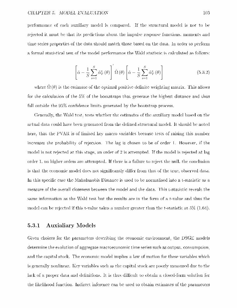
CHAPTER 5. MODEL EVALUATION 103
performance of each auxiliary model is compared. If the structural model is not to be
rejected it must be that its predictions about the impulse response functions, moments and
time series properties of the data should match those based on the data. In order to perform
a formal statistical test of the model performance the Wald statistic is calculated as follows:
[α− 1
S
S∑s=1
αsT (θ)
]′Ω (θ)
[α− 1
S
S∑s=1
αsT (θ)
](5.3.2)
where Ω (θ) is the estimate of the optimal positive denite weighting matrix. This allows
for the calculation of the 5% of the bootstraps that generate the highest distance and thus
fall outside the 95% condence limits generated by the bootstrap process.
Generally, the Wald test, tests whether the estimates of the auxiliary model based on the
actual data could have been generated from the dened structural model. It should be noted
here, that the PVAR is of limited key macro variables because tests of raising this number
increases the probability of rejection. The lag is chosen to be of order 1. However, if the
model is not rejected at this stage, an order of 2 is attempted. If the model is rejected at lag
order 1, no higher orders are attempted. If there is a failure to reject the null, the conclusion
is that the economic model does not signicantly dier from that of the true, observed data.
In this specic case the Mahalanobis Distance is used to be normalised into a t-statistic as a
measure of the overall closeness between the model and the data. This t-statistic reveals the
same information as the Wald test but the results are in the form of a t-value and thus the
model can be rejected if this t-value takes a number greater than the t-statistic at 5% (1.64).
5.3.1 Auxialiary Models
Given choices for the parameters describing the economic environment, the DSGE models
determine the evolution of aggregate macroeconomic time series such as output, consumption,
and the capital stock. The economic model implies a law of motion for these variables which
is generally nonlinear. Key variables such as the capital stock are poorly measured due to the
lack of a proper data and denitions. It is thus dicult to obtain a closed-form solution for
the likelihood function. Indirect inference can be used to obtain estimates of the parameters

CHAPTER 5. MODEL EVALUATION 104
of the economic model. A common choice for the auxiliary model is a vector autoregression
(VAR) for the variables of interest. The choice of the auxiliary model exploits the fact
that the solution to a log-linearised DSGE model can be represented as a restricted vector
autoregressive moving average (VARMA) model and this can closely be represented by a
vector autoregressive model (VAR). VAR models are known as a useful tool for exploring the
dynamic interaction of multiple time series.
These models comprise equations explaining a small number of key macroeconomic vari-
ables where each equation includes the same set of explanatory variables, lagged values of all
the variables in the system. The VAR approach is useful in analyzing an observed economic
phenomenon without having a prior explanation for it. A simple two variable VAR(1) is
represented by
yt = β11xt−1 + β12yt−1 + εyt (5.3.3)
xt = β21xt−1 + β22yt−1 + εxt (5.3.4)
so that the path of yt is aected by current and past values of the sequence xt in
5.3.3 while xt is aected by current and past values of the sequence yt in 5.3.4. The
errors εyt, εxt are uncorrelated white noise disturbances of zero mean and constant variance.
The above system of equations can be re-written in a more general and compact form as:
A0Yt = A(L)hYt + εt (5.3.5)
Yt = A−10 A(L)hYt + A−10 εt
Yt = Ξ1(L)hYt + ηt
(5.3.6)
where Yt is a n × 1vector of endogenous variables, A0 is a n × n matrix of coecients,
L is the lag operator and A(L)h = A1L + · · · · · · + AhLh is the hthorder lag polynomial and
E(εtε′) = I provides the variance-covariance matrix of the structural innovations. Equation

CHAPTER 5. MODEL EVALUATION 105
5.3.5 is the structural model under the assumption that there exists restrictions on the matrix
A so as to identify the coecients. Equation 5.3.6 is the reduced form VAR. Notice that ηt are
composites of the white-noise processes εt and thus also have zero mean and constant variance.
This basic reduced-form VAR is unable to give a detailed structure of the relationship or
shocks, which is what the policymaker really wants to know. To identify the shocks hitting
the system and their impact on the economy, the model needs extra assumptions. The
outcomes of the VAR analysis largely depend on these assumptions and the identication
restrictions cannot be readily tested against the data and so shock identication remains a
highly controversial issue. A type of model that is not susceptible to this problem is the DSGE
model. In this case, economic theory is used to dene all the linkages between variables. The
tight economic structure solves the identication problem. However, since theory is never
able to fully explain the data, a VAR is considered to `t' the data better.
Sims (1980) pioneered VAR models as models summarizing the information given by the
data and as a tool for conducting various policy experiments. According to the Wold theorem
Wold (1954) any time series vector can be represented by a VAR under mild regularity
conditions. The main restriction imposed by the Wold theorem is that the VAR model
should go to innity if it is to be considered 'good'. 'Good' models are those which replicate
the conditional and unconditional moments and a VAR is used to summarize these. There
are numerous methods for selecting a lag length the simplest being the likelihood ratio. Using
a VAR(1)3 is considered a restricted version of some larger-dimensional model. To 'judge'
and compare a model's statistics, 68 or 95 percent bands for the statistics of the data are
used as in Christiano et al. (2005). Inferences on the quality of the model depend on whether
the model's statistics are inside or outside these bands for any number of variables chosen.
This is one simple approach to test a DSGE model. There is a tight relationship between
dynamic equilibrium models and VARs. The example given by Del-Negro and Schorfheide
(2006) connects to the procedure of indirect inference and helps to identify this relationship.
Suppose that the vector of the DSGE model parameters is xed. One can generate 1 million
observations from the DSGE model. This occurs from drawing a sequence of shocks and
3A model with n lags is represented by VAR(h).

CHAPTER 5. MODEL EVALUATION 106
put them into the model to obtain articial data. Next, a VAR is estimated with h lags
using the articial data. The estimated VAR is considered as an approximation to the
DSGE model having the property that its rst h autocovariances are equivalent to the rst
h autocovariances of the DSGE model. The greater the number of lags the higher is the
accuracy of the VAR approximation of the DSGE model. If this experiment is repeated
but with dierent vector of parameter values the estimation of a DSGE model is almost
like estimating a VAR with cross-equation restrictions. In even simpler words, to obtain a
simulated approximation to the binding function, choose a set of parameters for the economic
model and derive the law of motion implied by this set of parameters. Simulate data using
this law of motion, and then using OLS t a VAR to the simulated data. Indirect inference
chooses the parameters of the economic model so that the VAR parameters implied by the
model are as close as possible to the VAR parameters estimated using the observed time
series.
As in Canova, Finn, and Pagan (1994), there are other ways of testing DSGE theories.
Cointegration restrictions implied by an RBC model are driven by permanent technology
shocks and are imposed on a VAR and then tested by the standard tools. DSGE models
are considered to be too simple to capture the complex random and probabilistic nature of
the data. If one compares their outcomes with the observed data, the probability of making
meaningful inferences is low. The main characteristic of DSGE models is that they can tell a
story about how the economy responds and evolves after an exogenous shock. The direction
of the main macroeconomic variables might be easy to see but the magnitude of the impact
and the timing of the output responses is relatively uncertain. GMM estimations as well as
likelihood methods are weak in dealing with such issues. 4Examples of DSGE models tested
by a VAR include Dedola and Neri (2007). In a standard RBC model with habit formation,
they use a VAR with several macro variables and examine the tness of the model when
robust sign restrictions are imposed to identify technology shocks in the data. Pappa (2005)
present a sticky and a exible-price model with monopolistic competition and use a VAR
4GMM and simulation estimators can be tailored to focus only on those aspects where misspecication issmaller as for example the Euler equation or the great ratios. Maximum likelihood estimation and testingrequire that at least under the null, the whole model is correct.

CHAPTER 5. MODEL EVALUATION 107
with a number of macro variables to verify whether an RBC style model ts the data better
than a sticky price model.
This thesis constitutes a contribution to the application of the indirect inference method-
ology described above. Although DSGE models have been under test for many years, the
theory of nancial development and/or human capital has not been tested in such a way
before. This work has two main original pieces. The rst one is the introduction of human
capital and nancial development in a DSGE model to be tested via indirect inference. The
second is the use of a panel vector error correction model (PVECM) as an auxiliary model
-which is represented by PVAR in levels-. The need for a PVECM arises because the data
used for the purpose of analysis in this thesis is nonstationary. When examining one country,
a VECM is used to deal with nonstationarity. Handling non-stationarity is described in more
detail in subsection 5.3.2. As described in Chapter 4, voluminous research on the relation-
ship and/or causality between nancial development and growth has failed to deal with the
identication problem. The simple growth regressions suer from biases which lead to spuri-
ous results. However, this thesis on the one hand uses indirect inference within the concept
of nancial development theory as an original way to 'solve' the identication problem by
setting a well-dened structural DSGE model. On the other hand, the auxiliary model also
becomes original since it uses a number of countries. Thus this work deviates from the simple
VAR representation of the DSGE towards a relatively more complicated panel procedure.
5.3.2 Non-stationarity
Non-stationarity implies that some part of the data moves in a random unpredictable man-
ner each quarter. This behavior of the macroeconomic data creates ambiguity when making
predictions about the long term. Unit root models imply extremely dierent dynamic prop-
erties and the classical statistical tools are not able to help in testing the null. The consensus
amongst economists is that macroeconomic time series are near-unit-root processes and this
makes tests have low power. The usual way to abstract from this feature of macroeconomic
data is to remove the trend using a number of mathematical transformations including deter-

CHAPTER 5. MODEL EVALUATION 108
ministic or stochatic detrending and dierencing. Most commonly, tests of macroeconomic
models are done on stationarised data since any stationary series is easier to be predicted
(its statistical properties do not change over time). The Hodrick-Prescott (HP) lter is the
best known technique applied in non-stationary data in the real business cycle literature.
Although this lter seems to have withstood the test of time the criticisms remain. HP as
well as Band Pass (BP) lters are not based on the theories used in these models. They con-
centrate on the statistical properties of the data and deviate from information drawn from
the data which could potentially be essential for the model's t. The drawbacks of the HP
lter are described by Cogley and Nason (1993). Instead, using original data for determining
or testing economic long run relationships is superior in that it can explain deviations from
the steady time trends usually observed when in times of crises. The testing procedure of
indirect inference utilises the original data.
A VAR is still suitable in cases of nonstationarity since covariance stationarity although
convenient, is unnecessary. One solution could be to take rst dierences if all variables are
I(1). Thus, a VAR in growth rate appropriate. In the case of cointegrated series however, one
can transform a VAR into a vector error correction model (VECM) and to jointly estimate
short-run and long-run coecients from the data. The VECM is a safer option than the
dierenced VAR because the latter reduces the degrees of freedom and thus the information
about the long-run properties of the data. If the shocks are nonstationary5 then a VAR
in dierences may be needed. This is because a permanent productivity shock leads to a
production function which is not cointegrated. This may lead to a non-stationary path of the
disturbances in the VAR in levels. A plot of the disturbances is usually informative on their
stationarity. Breaks or outliers may be observed but most of the times a unit root behavior
is not indicated. Hence, a VAR in levels could be appropriate even if a time series yt looks
non-stationary. As Sims, Stock, and Watson (1990) claim, the estimates of VAR coecients
can be consistent even when unit roots are present.
In this case, a multi-country model is evaluated and thus a panel-data vector autore-
gression methodology is used (PVAR). This technique is a combination of a VAR where all
5This is usually the case with the productivity shock or nominal shocks (i.e. money supply shock).

CHAPTER 5. MODEL EVALUATION 109
variables are treated as endogenous with panel-data technique. The panel-data approach
allows for unobserved individual heterogeneity.
To reduce any non-stationary data into stationarity a rst-dierenced VAR can be used
as the auxiliary model or and a VECM that includes cointegration relations implied by
the DSGE model. In the class of structural models where the true model also belongs, the
endogenous variable vector yt can be written in the linearized form as a function of the lagged
vector y, a vector of exogenous variables x,z and of errors u.
yt = f (yt−1, xt, zt, ut) (5.3.7)
The assumption made is that x are non-stationary, I (1)variables with drift trends which
may be zero. The vector z contains I (0)variables with a (possibly non-zero) deterministic
trends. The error vector, u, contains I (0)error processes with zero means and deterministic
trends such that:
ut = γt+ µ (L) vt (5.3.8)
This implies that there are cointegrating relationships in the model that dene the trend
values of y as linear functions of the trends in these exogenous variables:
Ayt = Bxt + Czt + γt (5.3.9)
where
∆xt = α∆xt−1 + d+ εt (5.3.10)
and thus
xt = xt +α
1− α∆xt + dt (5.3.11)
and

CHAPTER 5. MODEL EVALUATION 110
zt = c+ φt+ a (L) εt (5.3.12)
yt = A−1 (Bxt + Czt + γt) (5.3.13)
The above sequence of equations help to dene a VECM as:
∆yt = Dεt + Eεt + Fvt − Γ (yt−1 − yt−1) (5.3.14)
5.3.3 Model Selection
This thesis builds a DSGE model (as illustrated in Chapter 6). Since the model is already
calibrated, indirect inference is used in the framework of evaluating the model instead of esti-
mating the model. To be more specic, the use of indirect inference is to test the calibration
rather than the model as the latter would imply using dierent shares for each country or
estimating to get to the 'best' possible parameters. It is worth noting however, that in the
rest of this thesis the expression 'testing the model' will be equivalent to 'testing the cali-
bration'. Sequentially, the auxiliary model is a window through which the calibrated model
is examined. There is a common structural structure for all countries and the question im-
posed is whether, on average, these countries respond to one cause (nancial development)
or another (human capital). The aim is to examine whether there is an average structural
model with common coecients which are chosen by calibration that can be captured by a
PVAR with also common coecients.
The PVAR, is chosen to include all the endogenous variables. In that case, the amount
of coecients necessary to be matched is large and the analysis becomes more complicated.
It is thus better to focus on the variables of interest. In this case the main interest is growth.
Therefore, if the behavior of say, export and consumption cannot be explained by the model
and thus the null hypothesis is rejected, then one goes on with an auxiliary model including
less variables. Some relationships, like the one of consumption and exports is a complex one

CHAPTER 5. MODEL EVALUATION 111
so unless someone is interested in testing the role of consumption there is no harm in exluding
these variables from the PVAR setting. In this thesis, the test is based on 3 variables and
increases to 5. If the model is rejected when 5 variables are included, no further variables are
included since the probability of the model being rejected increases by the complexity arising
as the number of matching coecients increases and the test becomes more stringent.
The order of the PVAR is also of importance here. For the combination of the variables
that lead to a rejection of the model at PVAR(1), the lag order does not increase any
further. However, for the versions of the PVAR(1) that the model is not rejected, the lag
order increases to PVAR(2) and the analysis is repeated.
5.4 Conclusion
This chapter introduced the reader to the concept of indirect inference. It provided a def-
inition of the method as rst described by Smith and described the aim of the method. A
detailed description of the method guides the reader into a step by step procedure and leads
to the evaluation of DSGE modelling. This chapter distinguishes between evaluation and
calibration methods and describes the diculties with the former as to justify the use of the
latter in the subsequent chapters. An introduction to the idea of auxiliary models is given
concentrating on VAR and VECM regressions. The reader is also introduced to the use of
non-stationary data and gets familiarised with the drawbacks of ltering techniques. The
idea of auxiliary model and its use in indirect inference is important if one is to understand
the subsequent chapters which use a panel VAR to conduct them aim of indirect inference.

Chapter 6
A Multiple-Country Real Business Cycle
Model
6.1 Introduction
This chapter follows the idea of non-stationary macroeconomics in a manner similar to David-
son, Meenagh, Minford, and Wickens (2010). Non-stationarity implies that some part of the
data moves in a random unpredictable manner each quarter. This behavior of the macroeco-
nomic data creates ambiguity when making predictions about the long term. The usual way
to abstract from this feature of macroeconomic data is to remove the trend using a number of
mathematical transformations including deterministic or stochatic detrending and dierenc-
ing. Most commonly, tests of macroeconomic models are done on stationarised data since any
stationary series is easier to be predicted (its statistical properties do not change over time).
The Hodrick-Prescott (HP) lter is the best known technique applied in non-stationary data
in the real business cycle literature. Although this lter seems to have withstood the test of
time the criticisms remain. HP as well as Band Pass (BP) lters are not based on the theories
used in these models. They concentrate on the statistical properties of the data and deviate
from information drawn from the data which could potentially be essential for the model's
t. The drawbacks of the HP lter are described by Cogley and Nason (1993). Instead,
using original data for determining or testing economic long run relationships is superior in
112

CHAPTER 6. A MULTIPLE-COUNTRY REAL BUSINESS CYCLE MODEL 113
that it can explain deviations from the steady time trends usually observed when in times
of crises. The aim of this chapter is to introduce the reader in a model which can be tested
using the original data. Section 6.2 sets up an RBC model. Section 6.3 describes the method
of calibration and the solution method of the model. Section 6.4 describes the computer
algorithm while Section 6.5 explains the simulation procedure and graphically describes the
motion of variables after a productivity shock (Impulse Response Functions, IRFs). Section
6.6 concludes.
6.2 Model
Consider an open economy economic model,M. The home economy is small and populated
by identical innitely lived agents who produce a single good which they use to consume
and invest. The rest of the world (or the foreign country) is large faced with the same
choices but is unaected by changes in the home country. At the beginning of period t, the
representative agent chooses to consume a commodity bundle, the amount of time she wants
to spend at work (and thus leisure) and the total amounts of factor inputs necessary for the
production of output to be realised. The household has the choice of withdrawing from its
normal work activities to be involved in an innovative procedure which raises productivity.
This can be done via either of the two channels; spending time on nding credit (nancial
development) or human capital. This setup is similar to Klette and Kortum (2004) or Lucas
(1988) where the agents abstract from work to be educated or as in Aghion and Howitt
(1998) where the role of R&D is emphasized. The agent is constrained by time availability
and the resource constraint. In period t the economy is hit by a number of random shocks.
Important assumptions include: a) perfect information (no market imperfection) b) ability
to access to capital (private credit) from the bank if desired for the purpose of investing and
innovating c) there is free goods trade but these do not enter the production function and
thus are exchanged as nal goods. The model in Section 6.2.1 is a general form of the model
where initially productivity is exogenous. It is later extended to include either nancial
development or human capital as driving forces of the productivity that make it endogenous.

CHAPTER 6. A MULTIPLE-COUNTRY REAL BUSINESS CYCLE MODEL 114
6.2.1 The Representative Agent
The aggregate consumption is a function comprised of domestic and foreign (imported) goods,
Ct = f(Cdt , C
ft
)(6.2.1)
All the prices are relative to the general price level Pt. Following Armington (1969) the
composite consumption utility index in the aggregator form
Ct =[γ(Cdt
)−ρ+ (1− γ)
(Cft
)−ρ]− 1
ρ(6.2.2)
where γ is the Armington weight attached to the home goods in the consumption function,
σ = 11+ρ
is the elasticity of substitution between the two intermediaries. While the Armington
aggregator is judged for forcing the specialization pattern in trade to be determined in advance
is useful in empirical applications (Kose, 2011). The Armington elasticity is an important
parameter in the international business cycle literature that attempts to nd the source of
the high frequency uctuations in macroeconomic aggregates. The consumer maximises the
expected lifetime utility in a stochastic environment subject to the budget constraint. Since
agents are assumed to be homogeneous, they are all faced with the same preferences,
U0 = maxct,Lt
E0
[∞∑t=0
βtu (Ct, Lt)
](6.2.3)
where β is the discount factor, Ct is the consumption in period t, Lt is the amount of
consumption spent on leisure time, E0 is the mathematical expectations operator. The
preference ordering does not depend on ′t′. We assume that u (C,L) is increasing in (C,L)
and is concave. The utility function is assumed to follow a time-separable utility functional
form similar to McCallum and Nelson (2000).
U0 (Ct, Lt) = θ0 (1− ρo)−1 φtC1−ρ0t + (1− θ0) (1− ρ2)−1 ξt (Lt)
1−ρ2 (6.2.4)

CHAPTER 6. A MULTIPLE-COUNTRY REAL BUSINESS CYCLE MODEL 115
where 0 < θ0 < 1, and ρ0, ρ2 > 0 are the substitution parameters. In other words, they show
the marginal utility of consumption and leisure respectively. In a Cobb-Douglas setting ρ0
and ρ2 would be zero. The seriesφt, ξt are the preference errors. Barro and King (1984) note
that time-separable preference ordering of this form would not restrict the sizes of intertem-
poral substitution eects. In other words, it doesn't restrict the elasticity of substitution
between consumption and leisure to be one where it implies the choice between the two be-
ing independent of relative prices. Past work and consumption don't inuence the current
and future tastes. However, such a utility function constrains the relative size of various re-
sponses such as those of leisure and consumption to changes in relative price and permanent
income. The authors argue though that the presumption that departures from separability
matters for the purpose of RBC analysis matters only for days and weeks and not for months
or years. Therefore, since macroeconomic analysis is concerned primarily with time periods
as quarters or years, time-separability of preferences is considered justied and a reasonable
approximation in this context.
The total endowment of time is normalised to unity such that
Nt + Lt + zt = 1 (6.2.5)
or
Nt = 1− Lt − zt
where Nt can be the amount of time spend in work and zt the amount of time spent in
the innovation process created by the access to credit or by expanding human capital skills.
It can be considered as the entrepreneurial activity that a household can undertake which
involves spending the time denoted as z. The representative agent's budget constraint is
Ct +bt+1
(1 + rt)+
bft+1(1 + rft
) = Πt + wt (1− Lt − zt) + bt + bft − πtzt (6.2.6)
where

CHAPTER 6. A MULTIPLE-COUNTRY REAL BUSINESS CYCLE MODEL 116
Πt = yt − (rt + δ)Kt − wt (1− Lt − zt) (6.2.7)
and
yt = AtK1−αt (1− Lt − zt)α (6.2.8)
where bft and bt are the foreign and the domestic bonds respectively, yt is output,πt is a
tax/subsidy (negative tax) on entrepreneurial activity. It can be thought of as a tax imposed
by the lack of either nancial dvelopment or human capital or as a negative tax by the
presence of either of the two. Π is the prots of rms passed on to the households. It
is exogenous to the household however and thus no rst order condition is taken with its
respect.
The consumers maximises the utility subject to the constraint
maxct,,kt,bt,b
ft ,Lt,zt
E0
∞∑t=0
βt[θ0 (1− ρo)−1 φtC
1−ρ0t + (1− θ0) (1− ρ2)−1 ξt (Lt)
1−ρ2]
+λt
Πt + wt (1− Lt − zt) + bt + bft − πtzt − Ct −bt+1
(1 + rt)−
bft+1(1 + rft
) (6.2.9)
to reach to the rst order conditions
∂L∂Ct
= 0 = βtθ0φtC−ρ0t − βtλt (6.2.10)
θ0φtC−ρ0t = λt
∂L∂Ct+1
= 0 = βt+1θ0φt+1C−ρ0t+1 − βt+1λt+1 (6.2.11)
θ0φt+1C−ρ0t+1 = λt+1

CHAPTER 6. A MULTIPLE-COUNTRY REAL BUSINESS CYCLE MODEL 117
∂L∂bt+1
= 0 = −βt λt1 + rt
+ βt+1Etλt+1 (6.2.12)
λt(1 + rt)
= βEtλt+1
∂L∂bft+1
= 0 = −βt λt
1 + rft+ βt+1Etλt+1 (6.2.13)
λt(1 + rft
) = βEtλt+1
∂L∂Lt
= 0 = βt (1− θ0) ξtL−ρ2t − βtλtwt (6.2.14)
(1− θ0) ξtL−ρ2t = λtwt
The rst equation shows that the marginal utility of domestic consumption is equal to
the shadow price of output. The last equation shows that the marginal disutility of labor (or
the marginal utility of leisure) is equal to the real wage; to the labour's marginal product.
Combining the rst order conditions yields the following:
(1 + rt) =1
βEt
(φtφt+1
)(CtCt+1
)−ρ0(6.2.15)
Lt =
(θ0
1− θ0
)φtξt
1
Cρ0t
wt
−1/ρ2(6.2.16)
or
wt =
(1-θ0θ0
)ξtφtCρ0t
Lρ2t(6.2.17)
and

CHAPTER 6. A MULTIPLE-COUNTRY REAL BUSINESS CYCLE MODEL 118
1 + rft1 + rt
= 1
This last equation shows that the real exchange rate is xed otherwise the purchasing
power condition would be proven so that the interest rate dierential is equal to the expected
change in the real exchange rate.
6.2.2 Endogenising Productivity
Productivity growth is assumed to be triggered by either the level of nancial development in
the country or by the government percentage share of education spending. The idea is that
growth is triggered by people choosing to be entrepreneurial in response to their incentives.
These activities can take the form of acquiring skills via education or by borrowing credit
for investing in their business plans. If the private credit to GDP is low in the economy,
people will lose the latter incentive and they might go for higher education instead. There-
fore, greater productivity is enhanced through the incentives people have to take a business
opportunity realised by either nancial development or human capital. Thus, subsidising or
imposing a negative tax on these should generate higher productivity. Each country has a
dierent level of total factor productivity and the choices of its citizens determine the rate
at which they raise this by diverting their time from normal work to productivity-enhancing
activity.
The growth of productivity is expressed as:
At+1
At= a0 + a1zt + ut (6.2.18)
where zt is the entrepreneurial activity,ut is the error process and a1 is the eect of the
entrepreneurial activity on productivity growth.
It is assumed that there is some innovative or entrepreneurial activity the household
undertakes which involves spending time z. The labour is withdrawn from 'normal' work
activities and uses this time for an activity that raises productivity. This activity is enhanced

CHAPTER 6. A MULTIPLE-COUNTRY REAL BUSINESS CYCLE MODEL 119
either by nancial development or human capital. The household must divert a specic
amount of time away from standard work into this growth enhancing activity. Thus, the
agent decides how much time to devote to z by maximising its expected welfare as above.
The rst order condition with respect to z is:
∂L∂z0
= 0 =
∞∑t=1
[λt∂yt/∂z0]
− λ0 (w0 + π0) (6.2.19)
The idea here is that z0 aects all future yt as it raises productivity at all future points
of time.
Equation 6.2.19 leads to 1
0 = E0
∞∑t=1
α1A0
A1
βtθ0φtytCρ0t
− λ0 (w0 + π0) (6.2.20)
from which z0 is obtained. This is the optimal value invested in activities enhanced by
either nancial development or human capital. So one can think of two such z for each case
where the causal factor changes such that zfd0 , zh0 . Since however the result will be the same,
zfd0 , zh0 = z0.
z0 =
E0
∑∞t=1 β
tθ0φtytCρ0t
λ0 (π0 + w0)
− α0 + u0α1
(6.2.21)
This can be used with equation 6.2.18 to nd that:
A1
A0
=α1
E0
∑∞t=1 β
tθ0φtytCρ0t
λ0 (π0 + w0)
(6.2.22)
Equation 6.2.22 is a description of entrepreneurs ability to make allowance for the pro-
ductivity growth already coming from other sources when they decide optimal eort. These
sources exactly oset in their decision and thus it is the entrepreneurs that determine pro-
ductivity growth. Note that now it is assumed that yt and Ct both being non-stationary
1This is obtained by dierentiating the Lagrangean above with respect to z0. Note that At is determinedby 6.2.18. Then, ∂yt
∂z0= ∂At
∂z0k1−αt (1− Lt − zt)α = yt
At
∂At
∂z0for t ≥ 1. Since At = At
A1
A1
A0A0 and At
A1is not
dependent on z0 then, ∂At/∂z0 = At/A1
(∂A1/A0
∂z0
)= At
A1A0α1. This implies that
∂yt∂z0
= ytA0
A1α1. This then
leads to equation 6.2.20.

CHAPTER 6. A MULTIPLE-COUNTRY REAL BUSINESS CYCLE MODEL 120
can be approximated by random walks so that E0yt+i = E0y0 and E0Ct+i = C0. Using the
information on λ0 and w0 from the rst order conditions and ommitting the second order
terms of the numerator in equation 6.2.22, it becomes:
A1
A0
=
α1β1−βθ0φ0
y0Cρ00
θ0φ0C
−ρ00
π0 +
(1-θ0θ0
)ξtφtCρ0t
Lρ2t
A1
A0
=
α1β1−βθ0φ0
y0Cρ00
Lρ20
Lρ20 θ0φ0C−ρ00 π0 + (1-θ0) ξ0C0
(6.2.23)
Linearising this leads to equation 6.2.24.
A1
A0
= ψ0 − ψ1
(π′
0 + co
)+ error0 (6.2.24)
where π′0 = Lρ20 θ0φ0C
−ρ00 π0.
The idea is that the tax on entrepreneurs consists of the particular imposts levied on
business activity as such. As mentioned earlier, this is a negative tax or a subsidy for
the presence of a well established nancial sector or a strong human capital sector. In an
economy where nancial development or human capital is a causal factor for growth, implies
that peoples' choice of z is made so that they generate growth instead of income. It is
worth noting that an increase in z is leading to a reduction in labour supply oering to the
production process. This eect is however assumed to be negligible as z is a very small
proportion of total labour supply.
6.2.3 The government
It is assumed that the government's expenditure of current output follows a non-negative
stochastic process such thatGt ≤ yt for all t. The variableGt denotes government expenditure
at t. A second assumption made is that government expenditure does not enter the agent's
objective function. In models of business cycles which incorporate expectations, the output
is always at the desired level. Agents internalize the information available up to current time

CHAPTER 6. A MULTIPLE-COUNTRY REAL BUSINESS CYCLE MODEL 121
t and maximise their welfare subject to their constraints. In this framework, the government
does not distort the decisions of the agent directly and thus any stabilization policies have
no eect on the consumer's welfare. This is a no-tax economy and thus the government
expenditure is nanced by issuing debt, bonds bt each period which pays a return next
period.
The government issues bonds each period and collects a return next period thus
Gt + bt =bt+1
(1 + rt)(6.2.25)
where bt is real bonds.
6.2.4 The representative rm
The representative rm buys labour and capital which are used as input factors in the pro-
duction function so that the present discounted stream of cash ows,V, is maximised in a
stochastic environment. The rm is constraint by the constant returns to scale production
technology.
yt = AtNαt K
1−αt (6.2.26)
where 0 ≤ α ≤ 1, Yt is the aggregate output, Kt is capital carried forward from period
t − 1 and At is the state of technology. The production function is concave satisfying the
Inada-type conditions so that the marginal product of capital or labour reaches innity as
the factors go to zero while it reaches zero as the factors go to innity.
limK→0
(FK) = limN→0
(FN) =∞
limK→∞
(FK) = limN→∞
(FN) = 0
The capital stock follows the perpetual inventory equation:
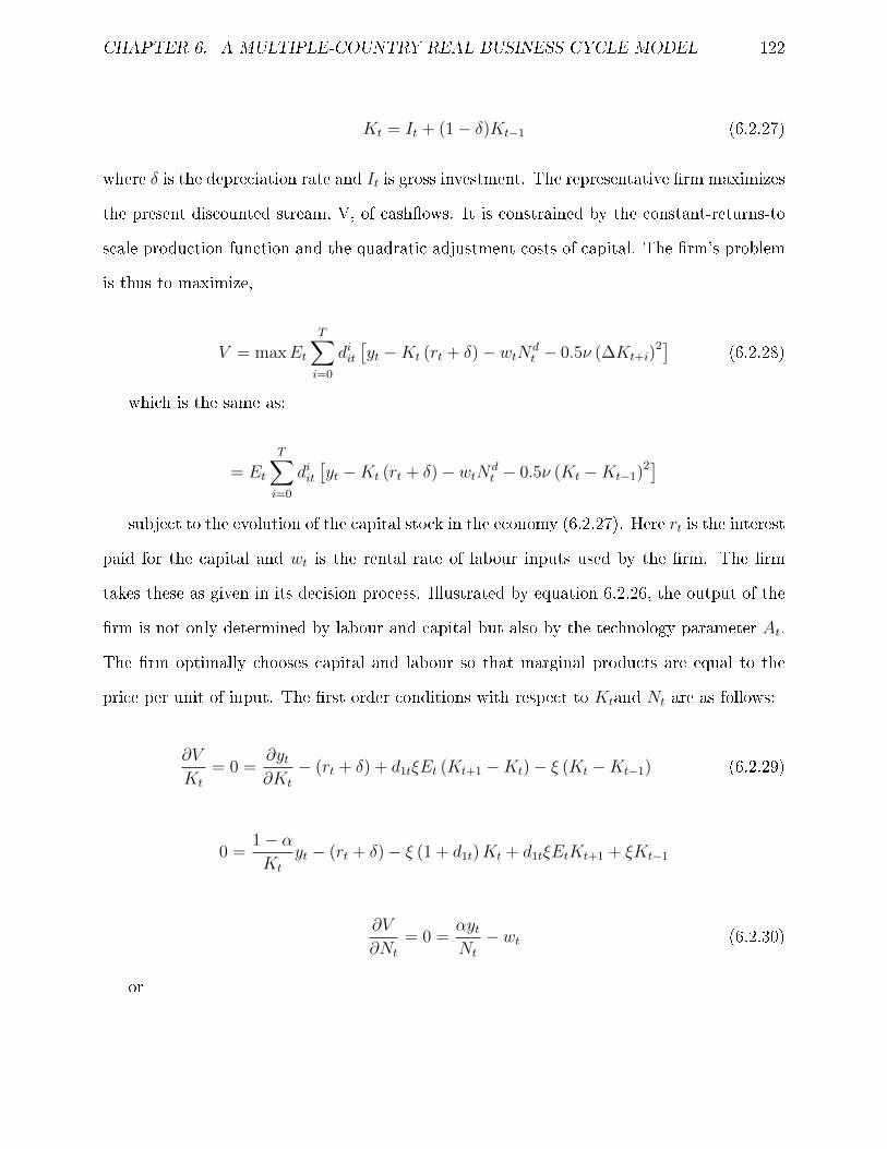
CHAPTER 6. A MULTIPLE-COUNTRY REAL BUSINESS CYCLE MODEL 122
Kt = It + (1− δ)Kt−1 (6.2.27)
where δ is the depreciation rate and It is gross investment. The representative rm maximizes
the present discounted stream, V, of cashows. It is constrained by the constant-returns-to
scale production function and the quadratic adjustment costs of capital. The rm's problem
is thus to maximize,
V = maxEt
T∑i=0
diit[yt −Kt (rt + δ)− wtNd
t − 0.5ν (∆Kt+i)2] (6.2.28)
which is the same as:
= Et
T∑i=0
diit[yt −Kt (rt + δ)− wtNd
t − 0.5ν (Kt −Kt−1)2]
subject to the evolution of the capital stock in the economy (6.2.27). Here rt is the interest
paid for the capital and wt is the rental rate of labour inputs used by the rm. The rm
takes these as given in its decision process. Illustrated by equation 6.2.26, the output of the
rm is not only determined by labour and capital but also by the technology parameter At.
The rm optimally chooses capital and labour so that marginal products are equal to the
price per unit of input. The rst order conditions with respect to Ktand Nt are as follows:
∂V
Kt
= 0 =∂yt∂Kt
− (rt + δ) + d1tξEt (Kt+1 −Kt)− ξ (Kt −Kt−1) (6.2.29)
0 =1− αKt
yt − (rt + δ)− ξ (1 + d1t)Kt + d1tξEtKt+1 + ξKt−1
∂V
∂Nt
= 0 =αytNt
− wt (6.2.30)
or

CHAPTER 6. A MULTIPLE-COUNTRY REAL BUSINESS CYCLE MODEL 123
wt =αyt
1− Lt − zt= MPL (6.2.31)
so that rms set wt equal to the marginal product of labor.
and thus
ν (1 + d1t)Kt = νKt−1 + d1tνEtKt+1 +1− αKt
yt − (rt + δ) (6.2.32)
Nt =αytwt
=
[wtαAt
]( 1α−1)
Kt (6.2.33)
6.2.5 The foreign sector
As Obstfeld and Rogo (1996) state, in open economies, a country's investment and con-
sumption plans are no longer constrained by its own production frontier but also by the
rest of the world production function. As in Armington (1969), demand for products in this
framework are distinguished not only by their kind but also by their place of production.
The Armington assumption that home and foreign goods are dierentiated purely because
of their origin of production has been a workhorse of empirical trade theory.
The foreign sector contains the import and export equations for the home country as well
as the current account position which is reected in the foreign bonds evolution equation.
The model contains 'trade equations'. The import and export equations of the home country
are as follows:
logCft = logIM = σlog (1− γ) + logCt (6.2.34)
logEXt = σf log(1− γf
)+ logCf
t (6.2.35)
The export equation shows that exports are a positive function of the total consumption in
the foreign country.

CHAPTER 6. A MULTIPLE-COUNTRY REAL BUSINESS CYCLE MODEL 124
In an open economy model, the home country and the foreign country agents need a
means of transaction to carry out the trading procedure. The foreign agents require home
money to buy home goods (i.e for their imports) and get foreign money from selling their
products (i.e. from their exports). The foreign country also sells foreign bonds to the home
country. So their net supply of foreign money is equal to net exports plus sales of foreign
bonds i.e. the balance of payments surplus. A similar story occurs in the home country such
that the net supply of the foreign country equals the net demand of the home country. The
home country gets foreign money from exporting their products to the foreign agents and
require foreign money for imports and purchases of foreign bonds. So if home agents adjust
their sales of foreign bonds then all balances. In equilibrium it is assumed that exports and
imports are equal and hence the agents have no incentive to change their asset position. In
disequilibrium any change between the domestic and the foreign bonds will depend upon net
exports,
NXt = EXt − IMt (6.2.36)
Foreign bonds thus evolve over time as follows:
bft =(
1− rft−1)bt−1 +NXt (6.2.37)
Finally, the goods market clearing position is
Yt = Ct + It +Gt + EXt − IMt (6.2.38)
6.3 Model Calibration and Solution
6.3.1 Model Calibration
The model is calibrated according to the work of Kydland and Prescott (1982), Obstfeld
and Rogo (1996), Orphanides (2003) and McCallum and Nelson (2000). It is a method

CHAPTER 6. A MULTIPLE-COUNTRY REAL BUSINESS CYCLE MODEL 125
constantly under scrutiny but it is a widely used method as an alternative to traditional
methods of analysing data in economics.2 The main characteristic of this method is that
instead of estimating them, the parameters of the model are determined by the long-run,
steady state behavior of the economy. These parameters are used for dening the model's
unconditional equilibrium distribution for the endogenous variables which is then compared
to that of the data. This method is an attempt to build theoretical models using parameters
that are chosen to ensure that the model is a good imitation of some particular characteristics
of the historical data observed (Hoover, 1995). Data are thus used to calibrate the model
economy so that it mimics the world as closely as possible. The main principle in the
calibration method is to use economic theory to be able to extract as much information as
possible from the data. In the calibration approach, theory helps in identifying the value of
the coecients and the measurements are used to give intuition to the theory (Cooley, 1997).
Calibration diers from estimation. As Kydland and Prescott (1996) state estimation at-
tempts to measure the size of something or to provide an approximate quantity of something.
To estimate a parameter, a researcher looks for a situation in which the signal-to-noise ratio
is high as to create statistical signicance. The data is combined with the theory and the
researcher constructs a probability model and developed an estimator that is robust enough,
relative to the parameter that is to be estimated and to features of the hypothesis made.
Calibration on the other hand, requires the search for constants that can be used to
satisfactory explain the economic behavior of macro variables under various circumstances. It
implies the use of parameter values from a variety of sources and other relevant econometric
studies and 'great ratios' which usually represent the shares in accounting identities such
as the share of labour in total revenue and of exports in GDP. The diculty arises when
information on the time-series data needs to combined with the information on the shares. 3
The DSGE models have become a means through which macroeconomic models are eval-
uated. There is now a reconcilliation between the short-run behavior (business cycles) and
2Many are against this method and choose to estimate rather than calibrate RBC models with methodssuch as Maximum Likelihood or Generalised Method of Moments. Examples include Altug (1989) andChristiano and Eichenbaum (1992).
3The dierences between estimation and calibration are explained in Cooley (1997).

CHAPTER 6. A MULTIPLE-COUNTRY REAL BUSINESS CYCLE MODEL 126
the long run behavior (growth). Using calibration implies specifying a model in terms of the
parameters chosen to capture the preferences, technology and institutional development. 4
The main justication for using calibration is that the estimates arising from econometric
models fail to give information on the deep structural parameters which is actually the main
focus of interest in RBC models.5 In order to generate simulations numerical values need to
be assigned to the structural parameters of the model as follows:
Table 6.1: Calibrated Values of the Coecients in RBC modelCoecient Value
α 0.70β 0.97
γ, γf 0.70δ 0.025θ0 0.5ρ −0.5ρ0 1.20ρ2 1.00σ, σf 1.00
The coecient of relative risk aversion (the fraction of elasticity of goods substitution) (ρ0)
is set at 1.2 and the substitution elasticity between consumption and leisure (ρ2) at unity.
The Armington weights(γ, γf
)are both set high at 0.7 and the elasticity of substitution
between the home and foreign consumption(σ, σf
)is set at unity to reect that the countries
competitiveness exists but it is not sensitive to the foreign alternatives. The calibrated values
are taken from micro-data estimates or from empirical characteristics of the economy under
examination. The parameters in the model have been calibrated to match the historical data.
Kydland and Prescott (1982) use the steady-state of the model as levels which ought
to match the sample averages of the main economic variables. The exogenous stochastic
processes should also be calibrated but it is a harder task concerning the lack of information
owing from the real economy. For example, it is hard to nd the stochastic structure of the
technology shocks or the shocks to the preferences. Therefore, AR (1) processes are assumed
4Wickens (1995) states that the main implication of RBC analysis is that the parameters associated withthe functions to be optimised i.e. preferences, technology, policy reaction functions and any other constraintsare structural.
5This is because, econometric models are expressed in terms of parameters that are functions of the deepstructiral parameters.
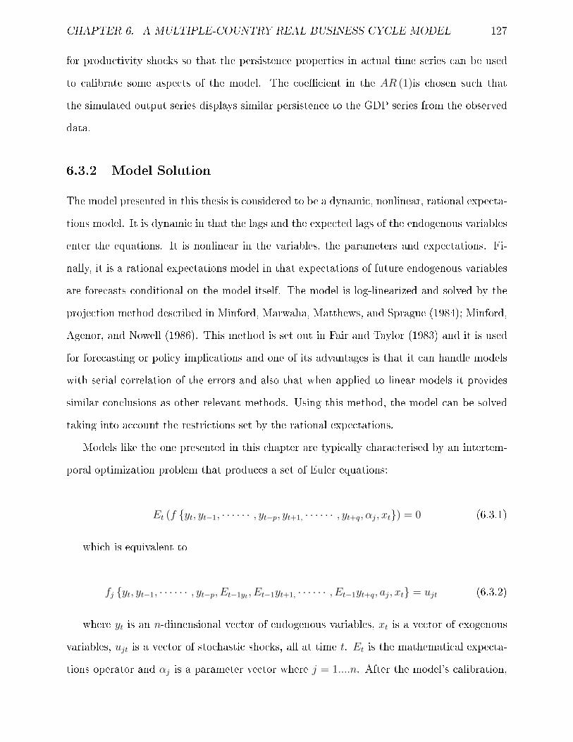
CHAPTER 6. A MULTIPLE-COUNTRY REAL BUSINESS CYCLE MODEL 127
for productivity shocks so that the persistence properties in actual time series can be used
to calibrate some aspects of the model. The coecient in the AR (1)is chosen such that
the simulated output series displays similar persistence to the GDP series from the observed
data.
6.3.2 Model Solution
The model presented in this thesis is considered to be a dynamic, nonlinear, rational expecta-
tions model. It is dynamic in that the lags and the expected lags of the endogenous variables
enter the equations. It is nonlinear in the variables, the parameters and expectations. Fi-
nally, it is a rational expectations model in that expectations of future endogenous variables
are forecasts conditional on the model itself. The model is log-linearized and solved by the
projection method described in Minford, Marwaha, Matthews, and Sprague (1984); Minford,
Agenor, and Nowell (1986). This method is set out in Fair and Taylor (1983) and it is used
for forecasting or policy implications and one of its advantages is that it can handle models
with serial correlation of the errors and also that when applied to linear models it provides
similar conclusions as other relevant methods. Using this method, the model can be solved
taking into account the restrictions set by the rational expectations.
Models like the one presented in this chapter are typically characterised by an intertem-
poral optimization problem that produces a set of Euler equations:
Et (f yt, yt−1, · · · · · · , yt−p, yt+1, · · · · · · , yt+q, αj, xt) = 0 (6.3.1)
which is equivalent to
fj yt, yt−1, · · · · · · , yt−p, Et−1yt , Et−1yt+1, · · · · · · , Et−1yt+q, aj, xt = ujt (6.3.2)
where yt is an n-dimensional vector of endogenous variables, xt is a vector of exogenous
variables, ujt is a vector of stochastic shocks, all at time t. Et is the mathematical expecta-
tions operator and αj is a parameter vector where j = 1....n. After the model's calibration,

CHAPTER 6. A MULTIPLE-COUNTRY REAL BUSINESS CYCLE MODEL 128
comes the model's solution.6 The solution aims to give the predicted current values of the
endogenous variables or the ex-post forecasts. In equation 6.3.1, solution implies a stochastic
process for yt. The incorporation of expectations leads to diculties in obtaining a practical
solution. A forward-looking solution sequence is calculated while initial and terminal con-
ditions are set that specify forecast values and expectations at the forecast horizon. The
non-linear dierence equations present, do not allow for a closed-form solution for each of the
endogenous variables. Iterative or indirect methods have been used to calculate the stochastic
process of the variables which corresponds to the solution. This means that one starts with
an initial approximation to a solution and then generate a number of better approximations
that converge to an exact solution.7
The programme development used for the solution of model guarantees that the model
solution is re-initialised instead of aborted when faced with problems such as taking logs of
negative numbers. If the expectations of future variables are somehow known then 6.3.1 is
a standard system of simultaneous equations. Common non-linear techniques such as the
Gauss-Seidel iterative process8 are used to solve the model repeatedly each time using a
dierent set of expectations. Solution is achieved every time values for variables in vector y
are provided. The number of iterations is increased until full convergence is ensured. This
also implies that the model's equations are to be equal with the model's forecasts as the
computer algorithm by Matthews and Marwaha (1979) ensures. As an example consider
information given for the year 1980q1 available to all agents. The algorithm initially guesses
a set of expectations and solves the model for 1980q2 onwards. It then checks whether the
expectations and the forecasts are equal. If not, then it changes the set of expectations until
convergence is reached.
6Some macroeconomists have attempted to algorithms to solve equation 6.3.1 in the non-linear case. Areview of these is given in Taylor and Uhlig (1990).
7The convergence as well as the speed of convergence is of interest here.8The Gauss-Seidel method is most widely used algorithm since it is simple and it always achieves conver-
gence for non-explosive models.

CHAPTER 6. A MULTIPLE-COUNTRY REAL BUSINESS CYCLE MODEL 129
6.4 Model Algorithm
The complexity and the non-linear form of the model require the use of a computer algorithm.
The nature of rational expectations models is such that the forward expectations terms tend
to create unstable roots. For a solution to be achieved however, stable roots or a saddlepath is
necessary. Terminal conditions are imposed to rst ensure that the transversality conditions
are met and secondly to ensure a stable path towards the convergence of rational expectations.
There are an innite number of consistent paths. To ensure that the stable path will be
chosen, the forecast values and the expectations at the end of the forecast horizon are set as
terminal conditions at equilibrium. In other words, for the unique stable path to be chosen,
beyond some terminal date, N , all expectational variables are set to their equilibrium values.
To avoid sensitivity of the model to variations in the terminal date, it i usually safer for the
terminal date to be 'large'. Although there are many other methods9, the long run equilibrium
condition of the model can be used to choose the terminal conditions as in Matthews and
Marwaha (1979).
The interative method of Gauss-Seidel is built in a programme called RATEXP developed
by Matthews (1979) and Minford, Marwaha, Matthews, and Sprague (1984). The programme
uses a dynamic programming technique (i.e. a backward-solving technique). However, the
solution vector is approached simultaneously for all t = 1, 2, ...T but convergence follows a
backward process. First, a dynamic solution of the model is reached for a given time span
and a given set of 'guesses' for the initial values of the expectational variables. These initial
values are used and adjusted in an iterative manner until convergence is obtained. When
the expectations become equal to the solved forecasts, the initial expectations set is slowly
altered until convergence is obtained. This is how expectational variables are endogenised in
that particular period. In a nutshell, the simple steps of the algorithm are
• 'Guess' a set of expectations
• Solve the model given this set
9In other cases, the steady-state properties of the model are used to choose the terminal conditions of themodel (Whitley, 1994).

CHAPTER 6. A MULTIPLE-COUNTRY REAL BUSINESS CYCLE MODEL 130
• Check for equality between expectations and solved forecasts
• Alter expectations until convergence is achieved
• Re-solve the model using the new values for the expectational variables
6.5 Model Simulations
In order to produce the sample of simulations desired (in this case 1000) a base run is rst
created which is simply set equal to the data. This becomes convenient to use after the
simulations are generated. To get the simulated data one needs to calculate the structural
errors. When the equations have no expectation terms, the structural error are simply
calculated as the dierence of the model from the data and are thus considered as the values
necessary to replicate the data. If the equations include expectations, the residuals are
estimated using McCallum (1976) and McCallum (1976) method of instrumental variables.
Here we use the lagged variables in a univariate time series processes for each expectational
variable. The structural residuals produce the shocks or the innovations which perturb the
model. In this case we have seven errors. Excluding the error coming from the production
function (the Solow residual), for each of the remaining six, a low-order ARIMA process is
estimated in order to determine their autoregressive behavior. For the productivity shock
the estimation is done on the dierences and it also includes the nancial development (FD)
indicator or the educational development (ED) indicator according to the theory tested.
The resulting innovations are then bootstrapped by time vector in order to preserve any
correlations between them. The shocks are thus drawn in an overlapping manner and added
into the model base run. For example, in period 1 a vector of shocks is drawn and is input to
the base run given its initial lagged values. The model is solved for period one and beyond
for all the future periods. In period 2, this becomes the lagged variable vector. For period 2,
another vector of shocks is drawn with replacement and added to the solution. The model is
then solved for period 2 and beyond and this becomes the lagged variable for period 3. This
process is repeated for period 3 onwards until 1000 simulations are completed and generated.

CHAPTER 6. A MULTIPLE-COUNTRY REAL BUSINESS CYCLE MODEL 131
This creates the bootstrap sample by the model's shocks.
The model was initially applied to each country separately. Then, it is necessary to
add these bootstraps on to the Balanced Growth Path (BGP) implied by the model and to
the trend terms in the exogenous variables and error processes. The BGP is found when
solving for the eect of a permanent change in each error/exogenous variable at the terminal
horizon T. The deterministic rate of change of this variable is then multiplied by this change.
This gives 1000 dierent scenarios of the economy's state over the sample period. These
bootstraps are then used for the estimation of a VECM; an auxiliary equation. When the
model is applied on all countries and the PVAR is the auxiliary model, the BGP is excluded
through estimation.
6.5.1 Impulse Response Functions: Productivity Shock
Once the model is solved, the model's implications are examined under the eect of one-o
rise of a number of variables. This is an opportunity to analyse the transition phase of the
model to its steady-state. One may consider the existence of such transition phase occurring
due to an initial position of the economy outside the steady state or a structural change which
changes the steady-state. This type of analysis is important when interested in evaluating
possible eects of change in policy interventions or in tastes and preferences. The usual way
to capture deviations from steady state is to have one or more of the exogenous variables being
perturbed and then compare this to the original, base, solution of the model. Therefore, an
impulse response function illustrates the deviations from the base after a demand or supply
shock is imposed which can be of a temporary or a permanent nature. The general idea of
impulse response functions (IRFs) is their ability to show how one variable responds over
time to a single innovation in itself or in another variable. Innovations in the variables are
represented by shocs to the error terms of the equations.
The length of the simulation period is an issue under debate. The chosen period needs
to be long enough so as to capture the eects of changes through the model. One needs to
be careful when setting the terminal date. The model's simulation should be unaected by

CHAPTER 6. A MULTIPLE-COUNTRY REAL BUSINESS CYCLE MODEL 132
the choice of the terminal date. For this reason, the terminal date should be suciently far
in the future. Moreover, a simulation over a long period of time is a necessary condition
for observing the model's long-run solution (Darby, Ireland, Leith, and Wren-Lewis, 1998).
The simulations for this model start in 1981, quarter 3 and end in 2007, quarter 4 for all the
countries. For the baseline simulation, the endogenous variables are set so that they capture
the historical values in an exact way. This is done by adding errors to each equation10. The
residuals are simply calculated as if the expected endogenous variables are equal to the actual
values and hence include not only the shocks to the equations but also the forecast errors.
What is of importance here is the eect of a permanent increase in the productivity by
1 standard deviation shock. A positive unanticipated increase in productivity encourages
higher output and increases permanent income through a reduction of the marginal costs.
The increase in output cannot occur without an increase in both, capital and labour. The
economy settles at a new permanently higher level of capital stock consistent with the higher
output. Capital however is slow to arrive and an increase in the real interest rate is necessary
to avoid any excess demand for the short-period limited supply. This explains the behavior
of the consumption and the capital stock in periods 5-38. Although real wages are increasing
in order to encourage labour to work more and increase production, the increase in the
real interest rate distorts consumption as well as the uncovered interest parity condition
which is restored with an increase in the real exchange rate. A high real exchange rate
makes foreign goods cheap relative to domestic goods, so net exports decline as the terms
of trade deteriorate. However, as the new capital stock arrives and becomes sucient, the
real exchange rate moves back to equilibrium causing an increase in the exports relative to
the imports. Moreover, as the real exchange rate is back to its equilibrium level, the higher
output is now sold at the foreign markets for a lower price. In this model, the income eect
does not seem to be strong enough to push the labour supply down and create an increase
in the real wage. As output increased, the prices in the economy fall. It can be explained by
the simple pricing method of rms. If the workers lose their wage bargaining power then the
prices set up by a mark up on the wage become lower together with the wage.
10See Appendix B.

CHAPTER 6. A MULTIPLE-COUNTRY REAL BUSINESS CYCLE MODEL 133
Figure 6.5.1: Impulse Response Functions for Increase in Productivity
0 20 40−0.05
00.05
Consumption
0 20 400
0.020.04
Output
0 20 40−0.05
00.05
Labour
0 20 400
0.010.02
Capital
0 20 40−0.05
00.05
Net Exports
0 20 400
0.020.04
Government Spending
0 20 400
0.010.02
Wage
0 20 40−1
−0.50
Bonds
0 20 40−1
01
ShC
onsumption
0 20 40−1
01
ShO
utput
0 20 40−1
01
ShLabour
0 20 40−1
01
ShC
apital
0 20 40−1
01
Shw
age
0 20 40−1
01
ShFD
0 20 40−1
01
ShED
0 20 409.19.19.1
x 10−3 Productivity
0 20 40−0.01
00.010.02
Financial Development Indicator
0 20 400
0.0050.01
Human Capital Indicator
Note: Shoutput stands for shock to output etc.
6.6 Conclusions
This chapter provides theoretically coherent micro-foundations for macroeconomic models
and constructs an econometrically testable DGE open economy model which is proposed to
calibrate using quarterly data on ten countries. The model is based on optimisation decisions
made by rational agents excluding money, taxes and unemployment benets. The reader
is guided through the rst order conditions of the consumer's and the rm's optimisation
problem which are used to derive the behavioural equations of the model. The world economy
is taken as given and all of the countries are considered as small open economies. Therefore,
in a safe way, only the domestic economy has a fully constructed model. It provided the

CHAPTER 6. A MULTIPLE-COUNTRY REAL BUSINESS CYCLE MODEL 134
calibrated values which drive the model's behavior and explained the reason of their use.
It then described the model solution by explaining the model algorithm and the model
simulations in detail. The chapter ends by a description of impulse response functions which
describe a shock of productivity and its impact on the rest of the variables. This conrms
that the model is working and thus one needs to set up an empirical model for testing. It is
the empirical issue that forms the basis for the next and last chapter.

Chapter 7
Testing a Multi-Country RBC model
I prefer to use the term 'theory' in a very narrow sense, to refer to an explicit dynamic
system, something that can be put on a computer and run
Robert Lucas (1989)
7.1 Introduction
The testing procedure described in Chapter 5 is used to test the model described in Chapter
6. The aim is to test whether there exists a relationship between nancial development
and growth or/and educational development and growth. Two theories of growth are set up
and each of them is tested via indirect inference. The chapter introduces the reader to the
data used, describes the auxiliary model and analyses the results. Section 7.2 describes the
data as well as the sources used to formulate the model. Section 7.3 explains in detail the
two theories representing the models under test while section 7.4 empirically evaluates the
auxiliary model and gives the reasons for the choice of the specic auxiliary model. Section
7.5 describes the testing procedure before providing the results in Section 7.6. Section 7.6
also explains Wald Statistic, the transformed Wald and the M-metric. Section 7.7 discusses
the results while Section 7.8 gives the IRFs from a shock to productivity. Section 7.9 provides
the results from four robustness tests and Section 7.10 concludes.
135

CHAPTER 7. TESTING A MULTI-COUNTRY RBC MODEL 136
7.2 Data
There are 10 countries in this study out of which 2 are developing. More developing countries
would be a further development. However, the limited availability of the data on the wages
and/or explosive AR(1) processes of the errors do not allow the use of them. Most of the data
on the macroeconomic variables is collected from the International Monetary Fund's (IMF)
International Finance Statistics database (IFS). The data collected consists of quarterly data
ranging from 1980q1 to 2007q4. Data availability ranges from 1960q1 to 2010q4. However,
for most of the countries the rst 20 years of data are not readily available and are thus
excluded from the sample. Moreover, to avoid internalizing the shocks caused by the 2007
nancial crisis, the sample also excludes the years after 2007q4. In the cases where quarterly
data is not provided by the IFS, the World Bank (WB) dataset is used to interpolate annual
data into quarterly data. Variables for the wage data is collected from UNESCO Institute
for Statistics. Only yearly data is available thus interpolation is used to create the sample
coverage data.
The nancial development indicator, private credit from nancial and non-nancial in-
stitutions to GDP is not widely available on the IMF database. The data source is Beck,
Demirguc-Kunt and Levine (Beck, Demirgüç-Kunt, and Levine, 2000) database available
from the WB. The indicator for human capital is the government spending to GDP ratio
and is collected from the IMF database. The unobservable variable, capital stock, is created
following Caselli (2004). The perpetual inventory equation is used:
Kt = It + (1− δ)Kt−1 (7.2.1)
where It is investment and δ is the depreciation rate. The initial level of capital is given
by:
K0 =I0
(g + δ)(7.2.2)
whereI0 is the value of investment in 1980q1 and g is the average geometric growth rate
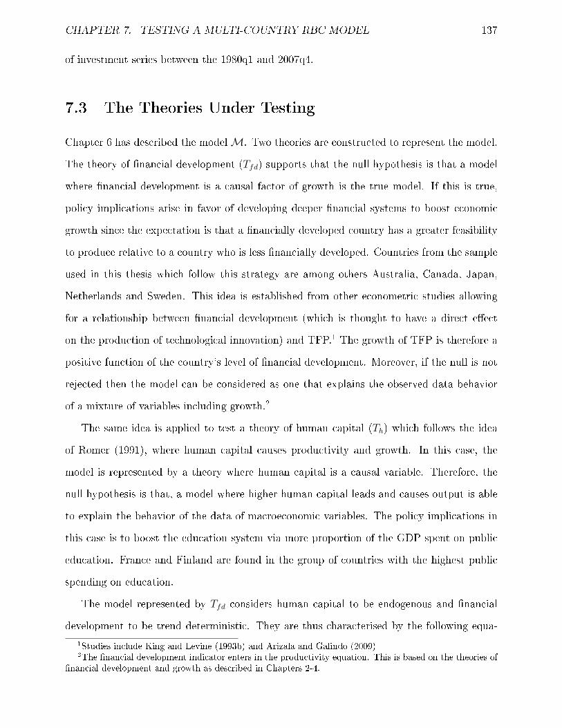
CHAPTER 7. TESTING A MULTI-COUNTRY RBC MODEL 137
of investment series between the 1980q1 and 2007q4.
7.3 The Theories Under Testing
Chapter 6 has described the modelM. Two theories are constructed to represent the model.
The theory of nancial development (Tfd) supports that the null hypothesis is that a model
where nancial development is a causal factor of growth is the true model. If this is true,
policy implications arise in favor of developing deeper nancial systems to boost economic
growth since the expectation is that a nancially developed country has a greater feasibility
to produce relative to a country who is less nancially developed. Countries from the sample
used in this thesis which follow this strategy are among others Australia, Canada, Japan,
Netherlands and Sweden. This idea is established from other econometric studies allowing
for a relationship between nancial development (which is thought to have a direct eect
on the production of technological innovation) and TFP.1 The growth of TFP is therefore a
positive function of the country's level of nancial development. Moreover, if the null is not
rejected then the model can be considered as one that explains the observed data behavior
of a mixture of variables including growth.2
The same idea is applied to test a theory of human capital (Th) which follows the idea
of Romer (1991), where human capital causes productivity and growth. In this case, the
model is represented by a theory where human capital is a causal variable. Therefore, the
null hypothesis is that, a model where higher human capital leads and causes output is able
to explain the behavior of the data of macroeconomic variables. The policy implications in
this case is to boost the education system via more proportion of the GDP spent on public
education. France and Finland are found in the group of countries with the highest public
spending on education.
The model represented by Tfd considers human capital to be endogenous and nancial
development to be trend deterministic. They are thus characterised by the following equa-
1Studies include King and Levine (1993b) and Arizala and Galindo (2009)2The nancial development indicator enters in the productivity equation. This is based on the theories of
nancial development and growth as described in Chapters 2-4.

CHAPTER 7. TESTING A MULTI-COUNTRY RBC MODEL 138
tions:
fdt = c+ γfdT + efdt
ht = µhyt−1 + eht
(7.3.1)
where fdt is the nancial development indicator and ht is the human capital proxy. The
coecients c, γ are estimated while the parameter µh is calibrated after regressions of this
form have been examined on a number of countries and found the general behavior of the
relationship between past levels of output and current public school expenditure. It thus
claims that past levels of output aect the government's decision to spend on education. In
other words, the level of income in a country is causing the level of public spending. Another
way of thinking about it is that public spending on education is a share past output with
some measurement error. The parameter µh is given a value of 0.25.
An environment like the one described by Tfd supports the idea that as the cost of nance
becomes less the economy's growth level is increased. The proxy used for fd is the private
credit from nancial and non-nancial institutions to the GDP. The economy is comprised
by homogeneous agents that have the opportunity to work and earn wages or they can visit
the bank for a loan which they can use for innovative purposes. The latter case leads to
an increase in productivity through the force of private credit owing within the economy.
The critical assumption here is that there are no explicit constrains in reaching credit within
economies. However, between countries, the level of nancial development is a proxy for
the access to credit. For instance, countries with higher ratio of private credit to GDP are
considered to be less nancially constrained. This model does not endogenize the banking
sector. It does not show the production function of the banking system. One could easily
add intermediaries with a credit production but the main point remains that any uctuation
in the economy is caused by productivity. The impact of banking or other factors is not to be
neglected but this thesis concentrates on a single key growth causal mechanism. This theory
is mainly exctracted from studies where one of the most widely used mechanisms through
which credit can have an impact on growth is the productivity channel (Schumpeter, 1912;

CHAPTER 7. TESTING A MULTI-COUNTRY RBC MODEL 139
Bagehot, 1873).
The second model represented by the human capital theory, Th follows Romer (1991).
In this environment, as the cost of education becomes less for the agent, there is a greater
incentive to get some time o work and spend time on gaining education. This enhances
higher long term economic growth levels through an eect on productivity growth. The agent
embodies knowledge which he/she trasfers onto innovative or productive ecient ideas. In
period t the economy is hit by a number of random shocks. Important assumptions include: a)
perfect information (no market imperfection) b) ability to use the education services provided
by the government if desired for the purpose of investing in education. When the human
capital becomes the main variable explaining growth, the nancial development equation
becomes endogenous. Thus the equations supporting the human capital theory are:
fdt = µfdyt−1 + efdt
ht = c+ γhT + eht
(7.3.2)
The parameter µfd is calibrated to be 0.006 after regressions are examined to establish a
relationship between past income and private credit. Theory, Th claims that private credit is a
function of past income. It is expected that a higher level of income in the economy positively
aects the level of credit owing in the economy (i.e. that nancial development is demand
driven). Like in Tfd parametes c, γ are estimated by OLS regressions. A model of human
capital claims that human capital development can explain growth and other macroeconomic
variables. The aim becomes to see which model does a relatively or absolutely a better job
in tting the data behavior and then conrm the eect of nancial development or human
capital development on economic growth via impulse response functions.

CHAPTER 7. TESTING A MULTI-COUNTRY RBC MODEL 140
7.4 The Auxiliary Model
7.4.1 Non-Stationary Data
The method of indirect inference has already been used for testing calibrated or already es-
timated DSGE macroeconomic model where the data are stationary (Le, Meenagh, Minford,
and Wickens, 2011). In this test procedure the residuals of the calibrated model are treated
as observable, are calculated from the given estimates and are allowed to be stationary or
non-stationary. A necessary condition for applying this test is that the auxiliary model is
chosen in such a way that the distribution of the test statistic has a good size and power prop-
erties. A testing method is required to have a 'reasonable' amount of power. That means
that it would not be useful if it rejects everything that is slightly not true or if it rejects
nothing at all. For the model under test, it is taken for granted that this testing method is
of both good size and power as indicated from other authors applying it to either stationary
(Le, Meenagh, Minford, and Wickens, 2011) or non-stationary data (Meenagh, Minford, and
Wickens, 2012).
A usual way in which DSGE models are estimated includes the ltering of macroeconomic
data as to make it stationary. As already explained, methods of ltering the data may
distort the dynamic properties of the model. Examples include the production of cycles
where possibly none exist. The disadvantages of the ltering methods lead to the use of the
original data when testing this model. The data generated by DSGE models are often non-
stationary. In this case, the model incorporates non-stationary exogenous technology shock in
the production function which generates non-stationarity. Other reasons for observing non-
stationary generated data include state variables (i.e. functions of predetermined variables)
depending on accumulated shocks or world income incorporated in the export function.
After linearising the model in Chapter 6, the assumption is that the solution of the model
can be represented by a vector error correction model for each country (VECM). Since the
technology shock is an unobservable non-stationary variable one or more of the long-run
structural equations will have a non-stationary residual. If the residuals calculated from the

CHAPTER 7. TESTING A MULTI-COUNTRY RBC MODEL 141
data and the calibration are treated as observables one can observe as many cointegrating
relations as endogenous variables. This allows the solution of the model to be represented as
a VECM in which the non-stationary residuals appear as observable variables. The VECM
can then be represented as a VAR. Levels VAR is more robust than VECM because it
can be used even when the system does not have stochastic trends and cointegration. The
VECM is constructed under the null hypothesis to make sure that it achieves cointegration.
As Meenagh, Minford, and Wickens (2012), state it would have been useful to test for the
existence of cointegration for each equation of the DSGE model. However, this is not possible
because a) any non-stationary residual is treated as a possible cointegrating variable and b)
a lack of cointegration would make the DSGE model impossible to be solved and thus no
simulations and no application of the Wald would be attainable.
7.4.2 Empirical Methodology of Panel Vector Autoregression (PVAR)
To accomplish the aim of ranking, accepting or rejecting a model an auxiliary model is built
to capture the dynamics oered by the model and represented by the two theories. Choices
of auxiliary models are usually a VAR, a VECM or a PVAR in the case of many countries.
The connection between VARs and DSGE models is made clear in Chapter 6. Working with
nonstationary series also implies the use of VECM which is re-written as a VAR in levels.
The idea of a PVAR in nancial development is established and empirically set in Love and
Zicchino (2002). A PVAR is the same as a VAR but is applied in a country level panel data
to study the dynamic relationship between countries' nancial development and economic
growth as well as countries' human capital development and growth. A VAR on panel data
aims at identifying the nancial development-growth and human capital-growth relationship
while allowing for xed eects (i.e. country specic unobserved heterogeneity in the levels of
the variables). A VAR also gives the opportunity for allowing country-specic time dummies
to capture aggregate country-specic shocks to macro variables that may aect all countries
at the same time.
In order to evaluate the model's ability in replicating certain characteristics of the data,

CHAPTER 7. TESTING A MULTI-COUNTRY RBC MODEL 142
a PVAR is built for a group of variables alone. It is not clear from other empirical studies
which variables are to be included in a PVAR and what order of lag oughts to be used. In
this case a PVAR of order 1 (PVAR(1)) is used with a group of three to ve variables. In
the case of a VAR, a limited number of macro variables and a lag order of one is preferable
because increasing either of the two increases the stringency of the overall test of the model.
In this case, if a model is rejected by a PVAR(1) no attempt is made to proceed to a stringent
test of based on a higher order PVAR. In general a VARMA is usually the representation of
a stationary loglinearised DSGE model. If the DSGE model is to be true, this means that
the true PVAR should be of innite order. However as Meenagh, Minford, and Theodoridis
(2008) note, raising the lag order of the PVAR worsens the t to the data probably due to
the complaxity in the bahaviour being captured.
The PVAR(1) takes the form:
ϑi,t = fi + Γ1ϑi,t−1 + δiT + ei,t (7.4.1)
where Γ1 is a vector of the country-common coecients on each macro variable which
are represented by the vector ϑi,t, fi is a vector of constants for each country to capture the
eects across units and δi captures country specic eects over time and T is time-trend.
The time trend is the Balanced Growth Path (BGP) for each country.
For any model under test, ϑi,t is either ve, four or three macro variable vector. The
choice of macro variables is described in table 7.1.
Table 7.1: Summary of PVARsTfd Th
PVAR 1 c, y, nx,A, fd c, y, nx,A, hPVAR 2 c, y, A, fd c, y, A, hPVAR 3 , y, A, fd y, A, hPVAR 4 c, y, nx,A, fd, h c, y, nx,A, fd, hPVAR 5 c, y, A, fd, h c, y, A, fd, hPVAR 6 y, A, fd, h y, A, fd, h
The abbreviations are for c:Consumption, y:Output, nx:Net Exports A: Productivity fd:Financial Development and h: human capital.

CHAPTER 7. TESTING A MULTI-COUNTRY RBC MODEL 143
Six dierent versions of a PVAR are set up for each of the theories under examination. For
example, for the purposes of testing the model represented by, Tfd, the vector ϑi,t in version 1
includes ve variables;yi,t, ci,t, nxi,t, Ai,t, fdi,t , while for Th, ϑi,t will be a ve variable vector
yi,t, ci,t, nxi,t, Ai,t, hi,t. By applying the VAR procedure to the panel data the assumption
is made that the underlying structure is the same for each country. However, this is not the
case in practice and to overcome this restriction xed eects are introduced, fi. Equation
7.4.1 implies that the error term satises the orthogonality condition so that the following is
true:
E [ϑi,tei,t] = E [fiei,t] = 0 (7.4.2)
The procedure followed includes opening up the vector to treat each equation separately
on all the sample countries. As an example, lets consider the case where ϑi,t = yi,t, Ai,t, fdi,t.
The idea is to rst take the actual data and apply the following equations using OLS on the
balanced panel data:
yi,t = f1,i + γ11yi,t−1 + γ12Ai,t−1 + γ13fdi,t−1 + δ1,iT + e1i,t (7.4.3)
Ai,t = f2,i + γ21yi,t−1 + γ22Ai,t−1 + γ23fdi,t−1 + δ2,iT + e2i,t (7.4.4)
fdi,t = f3,i + γ31yi,t−1 + γ32Ai,t−1 + γ33fdi,t−1 + δ3,iT + e3i,t (7.4.5)
The 10 sample countries thus share the same parameters except the constant the the time
trend where each country has its own. This trend variable can serve as a proxy for a variable
that aects the dependent variable but is nevertheless not directly observable although it
is highly correlated with time. In this case it captures the change in output with respect
to time. This eect is dierent for each country and thus dummies are used to capture the
uniqueness of the trend variable across countries.
CHAPTER 7. TESTING A MULTI-COUNTRY RBC MODEL 144
Running equations 7.4.3 to 7.4.5 on the data will give a set of 9 parameters.3
In this case, the data vector will be
Γ1 = [γ11, γ12, γ13; γ21, γ22, γ23; γ31, γ32, γ33]′
The next step is to apply these equations, separately on every single simulation. The
simulation matrix will be similar of size n × k where n is the number of simulations and k
is the number of parameters. In this case such a procedure will provide a vector of 9000
coecients. The same procedure is done for all the dierent combinations of macroeconomic
variables included in the PVAR. Each version is then tested by comparing the data coecient
vector to the simulation coecient vector via the M-metric.4
For versions 1 to 3, the model represented by Tfd is supporting that h is irrelevant and
thus left out while Th supports the same idea for the variable fd. There is a further attempt
to include both variables fd and h in the same PVAR which becomes even more demanding.
The power of the model increases as it has to match more details. For example, under version
1 vector ϑ becomes yi,t, ci,t, nxi,t, A, fdi,t, hi,t. The idea is to collect the relevant coecients
from each version and establish explanatory relationships between the three main variables
of interest; y, fd, h. The expectation is that the simulation coecients from versions 3 and 6
will be closer to the data.
7.5 The Testing Procedure
The explanatory power of the model described in Chapter 6,M, is empirically tested via
the method of indirect inference implemented on the full original, non-stationary data. By
applying the method of indirect inference on this model of non-stationary economic behavior,
the hope is to provide a place for nancial development and/or education development as a
determinant of growth through an impact on productivity. The model,M is applied to ten
3The constnat and the parameters on the trend are not of interest when calculating the Wald and arethus ignored.
4More details on the M-metric will be given below.

CHAPTER 7. TESTING A MULTI-COUNTRY RBC MODEL 145
countries which are all given the same calibrated values for the parameters in the structural
model. It is set up as a null hypothesis under which it is considered the true model in the
sense that it provides a true description of the data behavior so that its structural residuals
are also the true errors.
There are two sets of data for each country. The rst set describes the original data
while the second set is the simulated data. The auxialiary models are chosen for the original
sample data so that they describe the data eciently and closely. As already mentioned, the
auxiliary model used here is initially a PVAR with consumption, output, technology, nancial
development or educational development (or both) as the endogenous variables. The PVAR is
augmented to include net exports and also reduced to only output, productivity and nancial
development or educational development (or both) as alternative tests of the model. In order
to understand the implications of the model M about the data on any of the theories T ,
the auxiliary models are estimated on each of the pseudo-samples generated from the model.
This provides a distribution of the PVAR's parameters according to the structural model.
The aim is to compare the performance of the auxiliary model based on the observed data
with its performance when applied on the simulated data derived from the given distributions
of the parameters. Therefore the test is whether the PVAR estimated on the actual data
samplies lies within this distribution created from the PVAR on the simulated data at some
level of condence (95% in this case). This is done for both theories so that conclusions can
be drawn on which theory matches the data behavior best.
The PVAR acts as a vehicle with which the structural model is estimated and the null
hypothesis is either rejected or accepted. The question is: is it possible for T to have been
generated my M? To answer this question a test statistic based on the distributions of
the parameters of the auxiliary model is used. The criterion used is represented by a Wald
statistic which captures the dierence between the vector of relevant PVAR coecients from
the simulated and actual data. Under the null, the PVAR estimates based on the simulation
data will not be signicantly dierent from the PVAR estimates based on the actual data.
Each log-linear equation5 is augmented by an error whose unit root properties are tested.
5Each equation is shown in Appendix B.

CHAPTER 7. TESTING A MULTI-COUNTRY RBC MODEL 146
The residuals extracted from the AR(1) processes represent shocks or innovations entering
the model which are considered to be the ones generating the data. In a simple framework
consider the following equations:
Data = Model + et (7.5.1)
et = ρet−1 + ηt (7.5.2)
So the model,M is made up of a number of equations 7.5.1. The number of such equations
equals the number of endogenous variables. Not all equations are given an error term as there
is no need to do say in te case of equalities. 6 The error term et are ommited variables and are
modelled by AR(1) process as in 7.5.2. The residuals ηt are iid shocks and they are used as
time vectors from which errors are drawed with replacement and put into the error processes
(7.5.2) which are in turn put into the model (7.5.1). The DSGE model is bootstraped with
these shocks and 1000 bootstrap simulations of the data are generated which represent what
the implied model and its shocks have generated for the sample period of the data.
7.5.1 The Wald Test
In order to create the joint and individual distributions of the parameters of the PVAR
implied by the model, the PVAR estimation is carried out on each bootstrap sample. This
gives 1000 estimates which provide the sampling distribution under the null hypothesis and
the 95% condence intervals. The sampling distribution for the Wald test statistic is used as
a critical judge of the model. The Wald computes the joint distance of the data coecients
from the mean of the simulation distribution. As described in Chapter 5 this distance is
represented by:
Wald =[α− αsT (θ)
]′Ω (θ)
[α− αsT (θ)
](7.5.3)
6Also the an the productivity error term is captured in growth instead of levels and the fd or h variableis included as shown in Appendix B.

CHAPTER 7. TESTING A MULTI-COUNTRY RBC MODEL 147
In this case, α is the set of coecients supplied by the PVAR using the observed data
while ˜αsT (θ) is the mean of the VAR coecients found in the 1000 simulated samples. The
idea of the test is usually represented by 7.5.1.
Figure 7.5.1: Bivariate Normal Distributions
−3−2
−10
12
3
−2
0
2
0
0.1
0.2
0.3
0.4
x1
Correlation=0
x2
Pro
babi
lity
Den
sity
−3−2
−10
12
3
−2
0
2
0
0.1
0.2
0.3
0.4
x1
Correlation=0.9
x2
Pro
babi
lity
Den
sity
The gure concerns the case of only two parameters of the auxiliary model being con-
sidered. It is an example of how the data is compared to the model predictions using the

CHAPTER 7. TESTING A MULTI-COUNTRY RBC MODEL 148
Wald test. Two cases are examined; one where the correlation between the variables is zero
and one where it is 0.9. The height of the diagram represents the density of the parame-
ter combinations across samples. The mountain represents the joint distribution generated
from the model simulations. Two points are shown on each graph. Lets consider point A
to be the real-data-based estimates of the two parameters. In the case of no correlation the
model succeeds in providing a sensible explanation of the real world. Here, the mean of
each parameter's distribution is constant no matter what the value of the other parameter
is. However, when there is a high and positive covariance between the parameter estimates
across samples the mountain seems to rotate in such a way that now the model seems to fail
in explaining the reality. Now the data falls far from what the model predicts. However, if
the real-data-based estimates are represented by point B then the hypothesis that the model
is generating the data is not rejected. More PVAR parameters may follow various kinds of
distributions but in general the idea remains that each pair of parameters will create ridges
-as described- in multiple dimensions.
The aim is to see which of the models represented by each theory is better at explaining
the data oberved (i.e. which model is point B). To reach a conclusion a 'directed' Wald
test is used. It is a restricted Wald statistic and evaluation is based on a more restricted
sets of features and provides answers concerning which features the model can capture and
which it cannot. The 'full' Wald test derives from the fact that the Wald statistic is based
on the full set of variables instead of a more limited set of variables. The Wald statistic is
represented by the percentile of the distribution where the actual generated parameters lie.7
This is reset as to have the 95% value of the variate at the same point as the 95th percentile
of the bootstrap distribution. For example, a number of 96 for the Wald implies that the
data generated features fall beyond the 95% contour of the joint distribution and thus the
model is rejected by the data at a 95% condence level.
The Wald statistic is transformed in a normalised t-value following the logic that the
square root of this statistic,√Wald, is the Mahalanobis distance. By adjusting its mean and
7More specically, it is calculated as the percentile band around the joint mean within which the datagenerated features fall in that joint distribution.

CHAPTER 7. TESTING A MULTI-COUNTRY RBC MODEL 149
standard deviation, this becomes a normalised t-value where the 95% point is 1.645, and is
used as a measure of the distance between the original and the simulated data.8 Wilson and
Hilferty (1931) transform a chi-square variable to the Z-scale so that their p-values closely
approximated. The reason for standardizing the values of a χ2 distribution is to allow the
statistical signicance of the statistics, or p-values, to be more approachable and conveniently
represented. Following Wilson and Hilferty (1931) the normalised Mahanalobis distance is
basically a t-statistic and is given as:
t =
[(2MD)1/2 − (2n)1/2
][(2MD95%)1/2 − (2n)1/2]
× 1.645 (7.5.4)
whereMD is the value of the Mahalanobis distance derived using the actual data;MD95%
is the value of the Mahalanobis distance corresponding to the 95% tail of simulated distri-
bution and n is the degree of freedom of the variant. This ensures that the Mahalanobis
distance is 1.645 whenever the MD coincides with the 95% critical value of the simulated
distribution.
7.6 Results
7.6.1 The Transformed Mahalanobis Distance
After each and every regression has been performed using STATA, the coecients are cal-
lected and the transformed Mahalanobis distance is calculated in Matlab. 9The results are
best described by looking at the transformed Mahalanobis distance (t-stat) for the dierent
PVARs estimated as described in Table 7.2.
8The√χ2 is a normal variable and thus the Mahalanobis distance is the square root of the Wald value.
The square root of a chi-squared distribution can be converted into a t-statistic by adjusting the mean andthe size. The way is normalised here follows Le, Meenagh, Minford, and Wickens (2012) so that the resultingt-statistic is 1.645 at the 95% point the distribution and thus anything falling beyond would lead to therejection of the model.
9The codes are available on request.

CHAPTER 7. TESTING A MULTI-COUNTRY RBC MODEL 150
Table 7.2: Results-PVAR(1)Tfd t-stat Th t-stat
PVAR 1 c, y, nx,A, fd 4.76 c, y, nx,A, h 2.93PVAR 2 c, y, A, fd 4.65 c, y, A, h 2.61PVAR 3 y, A, fd 0.39 y, A, h 0.63PVAR 4 c, y, nx,A, fd, h 3.73 c, y, nx,A, fd, h 3.03PVAR 5 c, y, A, fd, h 3.29 c, y, A, fd, h 2.37PVAR 6 y, A, fd, h 0.686 y, A, fd, h 1.241
Applying the above procedure to the DSGE model with nancial development and human
capital the conclusion is that the long run relationship between the macroeconomic variables
is slightly better explained by Tfd. The conclusion is formed after massively rejecting both
theories for all versions except for versions 3 and 6. Under the latter cases, a nancial
development model explains the data bahaviour for the specic subset of variables better
than a human capital model. The results are providing an answer to the following question:
How well does the calibrated model replicate the actual data? After the simulations are
obtained one wonders whether the model is good enough to give simulated data close to the
actual data. The hypothesis set is that if the structural model is correctly specied, the set of
parameters obtained from the PVAR should not dier signicantly from those obtained from
the auxiliary model using observed data. The null hypothesis is thus that the model under
test is the true model. Although only two out of six versions attempted are accepted, when
the two theories representing the model are ranked against each other Tfd seems to to do a
better job in replicating the data behavior relative to Th according to the testing procedure.
The starting point is a PVAR with ve variables. Up until version 3, the data coecients
dier between the two theories. Versions 1 to 3 are loose in terms of the number of variables
that the model oughts to explain. In versions 4 to 6, the model is under more pressure and its
power is higher. The expectations rise to a model which can explain not only the behavior
of growth but also the behavior of the opponent theory. In these versions, the coecient
vector occurring from the data is the same for both theories. The expectation is that the
Wald statistic gets lower as we reduce the number of variables that the model is trying to
explain. The less the number of coeents, the better the tness of the model since it has less
CHAPTER 7. TESTING A MULTI-COUNTRY RBC MODEL 151
job to do in terms of matching. The anticipations are realised. Version 3 does a better job
in explaining the behavior of the endogenous variables compared to all the other versions.
Similarily, the results from version 6, as expected, are not rejected in comparison with 4 and
5.
The analysis is concentrated on PVAR 3 and PVAR 6 as under both theories the null is
not rejected. The results thus indicate that both models in this specic DSGE setting do
not fail to capture the reality and are both able to explain observed relationships between
educational development and growth as well as nancial development and growth. The theory
of nancial development shows that the simulations are exremely close to the data which
conrms that growth could successfully be explained in a model of nancial development
as a driver of productivity. This by no means implies that educational development is not
important determinant of growth. This simply implies that for the selected countries, human
capital also seems to be justied as the main driver of productivity but the simulations are
further from the data when compared to a nancial development theory. Nevertheless, the
non-rejection here implies that the models are both true and thus not rejected as a causal
account of the facts against which they are being tested.
7.6.2 Condence Intervals
The challenge now is to ensure that a model of nancial development ts the data better.
The transformed mahalanobis distance (t-stat) is one indicator. One needs to look closer
at the lower and upper 95% bounds on the coecients from the simulations and observe
whether these include the real data estimate. These are demonstrated in tables 7.3 to 7.6.
The fth column identies whether the real data estimate falls in or out the bounds formed
by the simulation estimates. Table 7.7 gives the Wald percentiles as well as the p-values. As
already discussed, the former is an indicator which if it takes a value of 100 the model fails
to capture the actual dynamics. The Wald statistic is a measure of the distance between the
simulations and the data. The lower the Wald, the better job done by the model. A Wald
of 100 indicates that the observed parameter estimates lie on the 100% .contour., i.e. in the

CHAPTER 7. TESTING A MULTI-COUNTRY RBC MODEL 152
95% rejection region. The p-value is the probability that the model is not rejected by the
data. It is clear that a Wald of 100 will give a p-value of zero indicating that there are no
chances for the model not to be rejected 10.
Table 7.3: Version 3-Condence Intervals and Wald Statistic: Theory fdVariable 95% lower
bound95% higherbound
Real dataestimate
IN/OUT
yyyAyfdAyAAAfdfdyfdAfdfd
-0.0063384-0.337405-0.030895-0.0079599-0.39302-0.0569525-0.00771885-0.44377-0.045215
0.793771.441550.922520.773891.17140.922420.790011.220050.92221
0.618410.436770.0559450.190080.769180.0228180.0001793-0.00620340.9281
ININININININININ
OUT
Table 7.4: Version3-Condence Intervals and Wald Statistic: Theory hVariable 95% lower
bound95% higherbound
Real dataestimate
IN/OUT
yyyAyhAyAAAhhyhAhh
-0.0208635-0.16129-0.205955-0.019182-0.172455-0.219185-0.022013-0.154185-0.23032
0.984980.958310.941360.9896750.9560650.938930.9878850.9524150.944015
0.613050.443610.0214480.193720.76446
-0.0061089-0.0419960.0389430.98848
ININININININ
OUTIN
OUT
10The p-value is calculated as (100−Wald)/100

CHAPTER 7. TESTING A MULTI-COUNTRY RBC MODEL 153
Table 7.5: Version 6-Condence Intervals and Wald Statistic: Theory fd95% lowerbound
95% higherbound
Real dataestimate
IN/OUT
yyyAyfdyhAyAAAfdAhfdyfdAfdfdfdhhyhAhfdhh
-0.457245-0.924275-0.012781-0.00086405-0.83072-0.426480-0.90197-0.0129230-0.00088255-0.83694-0.417895-1.0271
-0.0153625-0.0008252-0.89115-0.408815
0.9861400.973221.03825
0.003556254.92170.9854650.9759651.071650.0034785.061950.9864250.9727051.0859
0.00342444.95470.986975
0.1002900.0104470.0605680.00066410.56180.91569
-0.00076530.014016-0.0002577-0.33280.0149220.989630.037690.00004830.0280960.0048705
INININININININININININ
OUTININININ
Table 7.6: Version 6-Condence Intervals and Wald Statistic: Theory h95% lowerbound
95% higherbound
Real dataestimate
IN/OUT
yyyAyfdyhAyAAAfdAhfdyfdAfdfdfdhhyhAhfdhh
-0.370045-0.79725-0.0312305-0.0013686-0.24624-0.30586-0.78677-0.0319025-0.0011514-0.28285-0.2675-0.87695-0.024635-0.0007048-0.325955-0.0358615
0.9884450.9509550.9352250.003903354.05010.9911250.9650250.93455
0.004043453.747550.9867750.9527450.93534
0.003656253.92830.934615
0.100290.0104470.0605680.00066410.56180.91569
-0.00076530.014016-0.0002577-0.33280.0149220.989630.037694.83E-050.0280960.0048705
INININININININININ
OUTIN
OUTININININ
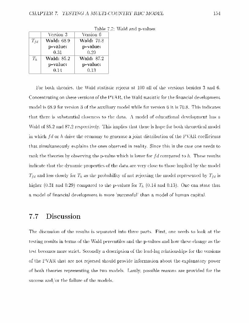
CHAPTER 7. TESTING A MULTI-COUNTRY RBC MODEL 154
Table 7.7: Wald and p-valuesVersion 3 Version 6
Tfd Wald: 68.9p-value:0.31
Wald: 70.8p-value:0.29
Th Wald: 85.2p-value:0.14
Wald: 87.2p-value:0.13
For both theories, the Wald statistic rejects at 100 all of the versions besides 3 and 6.
Concentrating on these versions of the PVAR, the Wald statistic for the nancial development
model is 68.9 for version 3 of the auxiliary model while for version 6 it is 70.8. This indicates
that there is substantial closeness to the data. A model of educational development has a
Wald of 85.2 and 87.2 respectively. This implies that there is hope for both theoretical model
in which fd or h drive the economy to generate a joint distribution of the PVAR coecients
that simultaneously explains the ones observed in reality. Since this is the case one needs to
rank the theories by observing the p-value which is lower for fd compared to h. These results
indicate that the dynamic properties of the data are very close to those implied by the model
Tfd and less closely for Th as the probability of not rejecting the model represented by Tfd is
higher (0.31 and 0.29) compared to the p-values for Th (0.14 and 0.13). One can state that
a model of nancial development is more 'successful' than a model of human capital.
7.7 Discussion
The discussion of the results is separated into three parts. First, one needs to look at the
testing results in terms of the Wald percentiles and the p-values and how these change as the
test becomes more strict. Secondly a description of the lead-lag relationships for the versions
of the PVAR that are not rejected should provide information about the explanatory power
of both theories representing the two models. Lastly, possible reasons are provided for the
success and/or the failure of the models.

CHAPTER 7. TESTING A MULTI-COUNTRY RBC MODEL 155
7.7.1 The Wald Percentiles and p-values
For clarication purposes one needs to understand what the regressions imply. The rst three
versions test each model in terms of whether it can generate the behavior of the economy and
also of the driver exogenous variables whether this is nancial development or human capital
indicators. However, version 4-6 become more demanding an asks the model to generate
the behavior of the non-driver variable. The question under versions 4-6 is whether the
driver model accounts for the economy's behavior and also the the behavior of the non-driver
variable. These versions are thus considered more demanding since the models do not have
a theory for the non-driver variable and the only information given is that this variable is
driven by the lag economic activity of the country.
For all versions except 3 and 6, both models are rejected as the true models and give
a Wald of 100. Thus the probability that the model is not rejected as the true model is
zero. This can be explained via the increase in the power of the model as more variables are
included. Notice how the t-stat falls as the number of variables in the PVAR are reduced
from version 1 to 6. Therefore, the more the number of variables (and the higher the PVAR
orders), the results worsen. The rst of each set consists of a wide range of variables which
includes consumption and exports. Both models perform badly. When the second of each set
eliminates net exports the power of both models decreases as the t-stat falls but none of the
models can be considered as the true one. Version 3 includes only the output, productivity
and the driver (while for version 6 it also includes the non-driver). Only then the Wald
is relatively lower and the p-value is relatively higher for both models. This is consistent
with other work on DSGE models conrming their weakness in accouting for a full range of
variables relative to a smaller subset of key variables. Typically, a macroeconomic model is
of interest for economists if it can replicate the behavior of the key macro variables which in
this case are output, productivity and the driver variable. Using this information together
with the Wald and p-values, none of the models is rejected although Tfd seems to perform
better.

CHAPTER 7. TESTING A MULTI-COUNTRY RBC MODEL 156
7.7.2 Lead-Lag Relationships
To get closer to the 'truth' the lead-lag relationships are reviewed to examine which are
the macroeconomic relationships that can be captured by each model. As the number of
relationships explained by the theory increases, the model is considered better. The model of
nancial development represented by Tfd as well as the model of human capital represented
by Th match the behavior of a subset of key variables from among the full test. So there are
a subset of variables that these models, can explain and others they cannot. Theory Tfd is
not far away from the dynamic properties it implies. In other words, the model's simulation
and the actual data do not fall far away and it does not fail to pick up lagged responses
at the individially coecients level. This implies that model predicted correlations among
three and four key macroeconomic variables are closer to actural data in a model where the
economy is driven by the levels of nancial development.
To simplify the discussion the PVAR is written to include only the 9 coecients of inter-
est.11 The results in Table 7.3 are an indicator of the model's performance with the following
set of equations:
yi,t = β11yt−1 + β12At−1 + β13fdt−1
Ai,t = β21yt−1 + β22At−1 + β23fdt−1
fdi,t = β31yt−1 + β32At−1 + β33fdt−1
where the coecient β11 is read as yy on the tables and β32 is fdA and so on. The results
in Table 7.4 come from the same pattern of equations but with h in the place of fd. Looking
at 7.3, while most of the real-data-based estimates of the PVAR coecients are individually
captured by the 95% bounds implied by the model simulations the nancial development's
response to its own lagged value is found to exceed its corresponding upper bound. Table 7.4
11The equations are for a PVAR version 3 of Tfd but one could do the same for Th.

CHAPTER 7. TESTING A MULTI-COUNTRY RBC MODEL 157
shows that the model with human capital as the driver fails to capture two relationships. The
response of human capital to lag output and its own lagged value exceed their corresponding
lower and upper bound respectively.
Tables 7.5 and 7.6 show how the models perform under the more strict condition implied
by version 6 as discussed above. The nancial development theory again performs better since
only one relationship is not captured by the model. The response of nancial development
to the lag human capital is above the 95% upper bound. That is to say that past human
capital does not explain the behavior of the nancial development or in other words, a model
where nancial development is the causal indicator, lagged human capital is not related to
nancial development. A model where the leading indicator is human capital fails to capture
the response of nancial development to lag productivity and lag human capital.
The main conclusion is that if nancial development is the driver of growth, it is possible
for its behavior not to be related to past output, productivity but rather output and produc-
tivity will be related to past nancial development. Also, human capital will be related to
past nancial development, output and productivity while these might not be related to past
human capital. The same idea follows if human capital is the causal variable where nancial
development is replaced with human capital. The dynamics of the important macroeconomic
variables are evident from both models. In other words, none of the models is poor in pre-
dicting any long run relationships occuring between past nancial development and human
capital and current growth or productivity and vice versa. However, a model where the causal
variable is nancial development can explain the behavior of the opponent theory while a
human capital model cannot.
7.7.3 The Success and the Failure of the Models
One can think of many reasons on the grounds of which the nancial development model fails
in the other versions. These results depend on the set of countries used. In this case, the set
of developed countries prevails. The failure of the fd theory could possibly be justied by
a non-linear, non-monotonic relatioship between nancial development and growth. Green-

CHAPTER 7. TESTING A MULTI-COUNTRY RBC MODEL 158
wood and Jovanovic (1990); Acemoglu and Zilibotti (1996); Khan (1999) describe the idea of
endogenousely emerging nancial institutions that have a positive but an unambigious eect
on growth. The magnitude of the eect depends on the level of economic or nancial devel-
opment of the country. Some research claims that the growth eect of nancial development
is unclear at low levels of development while it becomes positive as development expands.
The ambiguity may arise from adverse eects of nancial development on the propensity to
save(Obstfeld, 1994; Devereux and Smith, 1994) or from the negative eects that the adop-
tion of economic resources by the nancial sector has on growth (Deidda and Fattouh, 2001).
Another stream of research (Rioja and Valev, 2004) proposes that at low levels of nan-
cial development, additional development of the nancial market has an uncertain eect on
growth. At high levels of nancial development additional nancial development may have
a positive but a smaller eect on growth. Theoretically, the latter explanation could be used
to partly justify the rejection of the fd theory.
The distinction between the two theories can be explained by the nature and measure of
human capital. Firstly, human capital, unlike other types of capital, is not perfectly tradable.
This implies that its marginal product across individuals is not equalized and this gives rise
to aggregation problems and thus, aggregate output no longer depends merely on the average
level of the human capital, but also on its distribution. This leads to a second point. The
distribution of human capital is determined not only by individual ability but also by the
investment nancing opportunities. Thus with no or limited access to nance spending on
education by the government is not enough to drive the growth of the economy as this distri-
bution is an approximate determinant of the distribution of earnings. Thus, if a population's
abilities are normally distributed, a skewed distribution of education services would poten-
tially cause great welfare losses (Mincer 1974). Finally, to the extent that education is mostly
public funded, inequalities in education and human capital are largely structural inequal-
ities (as compared to market inequalities), which could have an unambiguous negative
impact on development(Easterly, 2007). Rajan and Zingales (2006) explain the persistence
of underdevelopment in the light that the elite and the already educated middle class will try

CHAPTER 7. TESTING A MULTI-COUNTRY RBC MODEL 159
to protect their rents by denying the poor of their education opportunities. Therefore, this
structural model needs to control for human capital inequalities if the eect of educational
development is to be captured completely (LIM and TANG, 2008).
7.8 Impulse Response Function: A Financial Develop-
ment Shock
The dynamic relationship among the proxy for nancial development and growth is examined
using IRF to demonstrate the eect of a positive one o shock to the private credit on
economic growth over time. Since the previous sections show that nancial development is
accepted as a causal factor of growth, the goal is to assess this role. The expectations is
that the variables considered to be more dependent on external nance would face sharper
increases from their steady states. As also expected, the results also show that TFP increases
as well.
The size of a nancial development shock whose is determined by the standard deviation
of the nancial development innovation series. Figure 7.8.1 demonstrates the results. As
expected the output, although innovations to nancial development do not initially aect
growth too much it eventually reaches a new permanent level. This is reecting the direction
of causality running from nance to growth. Moreover, there is also a positive eect on the
education proxy. This is again expected as education is considered to be a sector of the
economy which dependents on nance. The eect of consumption is captured solely through
the terminal conidtions of the model. It shows a small increase initially while it falls back
to zero at the the end. This is also a sign of consumption being driven by the nancial
indicator. Trade is a highly dependant sector on nance. The eect is the same as that on
growth indicating that nance leads to higher trade shares. Moreover, the capital sector is
nancially driven as implied by the permanent positive eect of a nancial shock. As a nal
conclusion from the IRFs, there is evidence of nancial development promoting economic
growth and productivity.

CHAPTER 7. TESTING A MULTI-COUNTRY RBC MODEL 160
Figure 7.8.1: Impulse Response Functions for Increase in Private Credit to GDP
0 20 40−5
05
x 10−3 Consumption
0 20 40−5
05
x 10−3 Output
0 20 40−5
05
x 10−3 Labour
0 20 40024
x 10−3 Capital
0 20 40−5
05
x 10−3 Net Exports
0 20 40−5
05
x 10−3Government Spending
0 20 40012
x 10−3 Wage
0 20 40−0.1
−0.050
Bonds
0 20 40−1
01
ShC
onsumption
0 20 40−1
01
ShO
utput
0 20 40−1
01
ShLabour
0 20 40−1
01
ShC
apital
0 20 40−1
01
Shw
age
0 20 40−1
01
ShFD
0 20 40−1
01
ShED
0 20 40012
x 10−3 Productivity
0 20 400
0.0050.01
Financial Development Indicator
0 20 40−2
02
x 10−3Human Capital Indicator
7.9 Sensitivity Analysis
In order to check the robustness of the results above three extensions are made. The rst
one involves repeating the analysis for the non-rejected models including two lags instead of
one lag in the PVAR. The second one is based on changing the calibrated values with which
the nancial development indicator and the human capital indicator aect the productivity
process. The third one imposes the same balance growth path on each country and the fourth
separates the countries into developed and developing and re-examines.

CHAPTER 7. TESTING A MULTI-COUNTRY RBC MODEL 161
7.9.1 Two-lag PVAR
As already stated in Section 7.6, the versions PVAR 3 and PVAR 6 are not rejected. The
same technique is repeated for running a PVAR(2) for each of these versions of the auxiliary
model. Table 7.8 indicates the results. Under this scenario, the number of coecients to
be matched increases. The causal model is reected through the coecients. For the 18
coecients case (PVAR 3), the results thus indicate the strength of nancial development
theory in explaining these coecients. A model where human capital is considered to be the
causal factor, is not capable of explaining these coecients beyond a lag order of 1.
When the auxiliary model becomes one with 32 coecients, (PVAR 6) both models fail
to capture the relationships of the variables included in the PVAR. The results indicate
that both of the models have nothing to say for the causal processes. The auxiliary models
presented in PVAR 6 are unable to explain the behavior of the variables involved. It is
however important to notice that the ranking is still in favour of the nancial development
theory. Although both models are rejected, the theory of human capital is rejected at a
bigger degree. The ranking remains the same whether one looks at PVAR 3 or PVAR 6
which is another indication of the nancial development theory being clearly distinguished
from the human capital theory. The individual coecients for both versions of the PVAR
the results indicate to the same conclusions as above. More than one relationship fails to
be captured in the case of human capital theory. A model with a causal force coming from
nancial development is able to explain more relationships relative to those that the human
capital theory can explain.
Table 7.8: Results-PVAR(2)Tfd t-stat Th t-stat
PVAR 3 y, A, fd 1.58 y, A, h 2.71PVAR 6 y, A, fd, h 2.26 y, A, fd, h 2.73

CHAPTER 7. TESTING A MULTI-COUNTRY RBC MODEL 162
Table 7.9: Wald and the p-valueVersion 3 Version 6
Tfd Wald: 95.0p-value:0.05
Wald: 95.1p-value:0.049
Th Wald: 95.4p-value:0.046
Wald: 95.7p-value:0.043
The Wald statistic for both theories is now higher compared to the analysis under one lag.
This indicates that the probability of each model not being rejected is reduced. However,
for version 3, the nancial development theory still indicates closeness to the data. A model
of educational development has a Wald of greater than 95. This implies that there is no
hope a theoretical model in which h drives the economy to generate a joint distribution of
the PVAR coecients that simultaneously explains the ones observed in reality. Since for
version 6, both theories are rejected, one needs to rank the theories by observing the p-value
which is higher for fd compared to h. These results indicate that the dynamic properties
of the data are very close to those implied by the model Tfd and less closely for Th as the
probability of not rejecting the model represented by Tfd is higher (0.05 and 0.049) compared
to the p-values for Th (0.046 and 0.043). One can state that a model of nancial development
is more 'successful' than a model of human capital.
Increasing the lag of the PVAR has not altered the ranking of the theories. However, both
models perform worse than before. Even for the version in which the nancial development
theory is not rejected the probability of this event is very low. Under this lag order the test
is more demanding and the results are expectable.
7.9.2 Calibration: The Productivity Process
In Appendix B, the equation for the Solow residual is represented as
At = At−1 + α1z + ufdt (7.9.1)
where z is either fd or h. For the analysis in sections prior to Section 7.9,α1was set to

CHAPTER 7. TESTING A MULTI-COUNTRY RBC MODEL 163
0.006 under the nancial development theory where as for the human capital theory it was
set to 0.05. In this section, the calibrated values for the two theories is reversed. Thus the
magnitude with which the two theories were set to aect the productivity process are now
reversed. The results are shown in Table7.9.2. Since for the rest of the versions of the PVAR,
both models are rejected only versions 3 and 6 are reported below.
Table 7.10: Results-Calibration ReversalTfd t-stat/Wald/p-value Th t-stat
PVAR 3 y, A, fd 1.34/94.7/0.053 y, A, h 2.30PVAR 6 y, A, fd, h 1.54/94.9/0.051 y, A, fd, h 2.13
Financial development theory seems to explain the relationships under both versions. A
model driven by human capital is rejected under both versions. This indicates that Tfd is not
as sensitive to the calibration changes as Th is. The conclusion remains the same. Under both
contexts (before and after the calibration reversal) a model driven by nancial development
fails to be rejected in either versions of the PVAR. However, a model with human capital as
the causal factor is rejected after the calibration reversal which is an indication of its failure to
explain the relationships demanded beyond the already calibrated values. The Wald statistic
and the p-value indicate that the probability of the human capital model not being rejected
is zero.
7.9.3 Common BGP
The above description depends on testing the model assuming that the Balanced Growth
Path (BGP) of each country is dierent. Another analysis is done where the restriction of all
countries sharing the same BGP is imposed. In this case the PVAR is described by equation
7.9.2.
ϑi,t = fi + Γ1ϑi,t−1 + δT + ei,t (7.9.2)
The same procedure is followed and the results are provided in Table 7.11. In this case
a model where human capital is the causal variable, is totally rejected. Versions 3 and 6 are

CHAPTER 7. TESTING A MULTI-COUNTRY RBC MODEL 164
Table 7.12: Wald Percentile/p-valuesVersion Wald Tfd p-value Wald Th
3 81.4 0.18 1006 87 0.13 100
1,2,4,5 100 0 100
again better in the sense that they provide the lowest trasnformed t-statistic but it turns out
that on these subsets of variables Tfd model is not rejected while Th is rejected in both cases.
Table 7.11: ResultsVersion Theory t− stat Reject/Do
not reject
1 TfdTh
4.01007.8453
RejectReject
2 TfdTh
3.00676.7055
RejectReject
3 TfdTh
0.84925.4236
Do notrejectReject
4 TfdTh
3.45446.4985
RejectReject
5 TfdTh
3.46725.6841
RejectReject
6 TfdTh
1.14345.2415
Do notrejectReject
In this case, the Wald percentile is 100 for all other versions except 3 and 6 for theory
Tfd. In contrast, the Wald percentile is 100 for all versions of the auxiliary model represented
by Th.
On an individual examination of the coecients showned by Table 7.13 and 7.14 the
results are not extremely dierent from the ones where the BGP for each country is dierent.
In this case, Tfd is not able to explain a relationship running from past productivity to
nancial development but the important thing is that is captures relationships that run from
nancial development to the rest of the variables. A model with human capital as a causal
factor cannot explain the eect of lagged human capital to output not to productivity as seen
in table 7.14. It thus fails to capture the main relationships that is expected to and hence

CHAPTER 7. TESTING A MULTI-COUNTRY RBC MODEL 165
the reason is rejected.
Table 7.13: Version 3-Condence Intervals:Tfd95% lowerbound
95% higherbound
Real dataestimate
IN/OUT
yyyAyfdAyAAAfdfdyfdAfdfd
-0.445635-1.26275-0.000622-0.063862-0.458355-1.25715
-0.00055125-0.061482-0.497765
0.99697500.9800250.00411575.90191.039250.975020.00424985.9630000.993975
0.0932570.00761620.00061170.63760.91406
-0.0014204-0.0002698-0.315260.010545
INININININININ
OUTIN
Table 7.14: Version 3-Condence Intervals:Th95% lowerbound
95% higherbound
Real dataestimate
IN/OUT
yyyAyhAyAAAhhyhAhh
-0.39782-0.060626-0.00118775-0.125815-0.405625-0.055867-0.00132515-0.647435-0.46114
0.988550.936350.00404554.33191.07640.9358550.00415914.162651.02095
0.0987710.0566340.0065490.562060.91580.93884-0.00257-0.332820.0056763
ININ
OUTININ
OUTOUTININ
What diers from the regressions with separate BGPs is that the long run relationships
cannot be explained by the educational development proxy.
Tfd passes the more stringent test and can explain the behavior of all macro variables in
the PVAR including that of the educational development. With a Wald percentile of 81.4,
the observed dynamics are not only individually, but also jointly explained by the theoretical
model Tfd. By using the `directed' Wald, examination of the theoretical model focuses on
the partial capacities in explaining the dynamics. The comparison of the structural model
with nancial development shows that if the model is restricted to human capital as a driving
mechanism of productivity and growth, then the model is rejected by the dynamic data. The
implication under these conditions that there is no hope at all for the theoretical model Th

CHAPTER 7. TESTING A MULTI-COUNTRY RBC MODEL 166
Table 7.15: t-statistic: Developed Vs Developing CountriesDeveloped Version 3 Version 6
fd 0.38 0.39h 0.43 0.96
Developing Version 3 Version 6fd 1.19 0.88h 1.75 1.88
to generate a joint distribution of the PVAR coecients that simultaneously explains the
ones observed in reality. In conclusion, under both cases, with or without a common BGP,
a model where nancial development is a causal factor of growth is superior to one where
human capital is a causal factor.
7.9.4 Country Group Results
As a robustness test, the sample is divided into developed and developing countries. The
sample is dominated by developed countries. Nevertheless, the results for developing countries
are very close to those for developed and to those on average. In terms of ranking the
two theories the results are the same. A theory of fd is better at explaining the observed
behaviours. The model represented by h in version 3 and version 6 of the auxiliary model
is rejected. One can conclude that the average type of analysis used in the main thesis is
correct since even when the sample is separated the results are not very dierent.
7.9.5 Financial Development or Human Capital: Why bother?
As indicated from the sensitivity analysis, a nancial development proves to be more stable
and reliable. The results indicate that the model of nancial development fails to be rejected
for all the cases under version 3 of the PVAR. The main conclusion is that, for the cases where
both models are rejected, the ranking is important but what is of even more importance is
the fact that both models have nothing to say about the causal processes. The human capital
model is rejected at more stages compared to the nancial development model. This tells us
that this model cannot explain the behavior of the variables in the PVAR. The main question

CHAPTER 7. TESTING A MULTI-COUNTRY RBC MODEL 167
of this thesis is whether on average these 10 countries respond to nancial depth or to human
capital investments. If there is an average structural model with common coecients that
can be represented by a PVAR then this is the nancial development model. None of these
models captures the exact causal process. However, the nancial development theory gives
a clearer picture.
From these tests, there is no policy implication in the sense of a rule that the policy maker
ought to follow. However, the non-rejection of the human capital model in comparison with
the human capital one is sending a message to the policy makers whose priority is growth,
that it is perhaps time to give more weight on the nancial depth of the country. Countries
like India, used have policies focused on the education and on increasing human capital.
After the 1990s with nancial liberalisation, India's growth rates expanded. This is only one
example which indicates the importance of nancial development. This thesis does not falsify
the human capital theory. Human capital remains an important cause of economic growth.
It is only when compared with nancial development on average that one ought to rethink
the place of nancial depth in economic models.
It also depends on the interests of the policy makers. As seen from the results, if a
policy maker is interested in consumption or net exports then none of these models are good
enough to be considered as the 'true' models for him/her. As indicated, both models fail to
capture complex relationships in ne detail. However, if the policy interest is growth then
the success of both models (i.e. the fact that they are not rejected) leads the policymaker to
pursue policies that focus on nancial development and growth. Since the fd model is more
successful relative to the h model, the policy maker could enhance nancial development
which will in turn feed back to growth.
7.10 Conclusion
This chapter introduced the reader to the data and gave an extensive description of the
auxiliary models representing the DSGE model under test. There are two models where
productivity growth is either caused by nancial development or human capital. The results

CHAPTER 7. TESTING A MULTI-COUNTRY RBC MODEL 168
indicated that a model where productivity is driven by nancial development is a better at
explaining the data behavior than a model where human capital is a causal factor. For every
structural causal process there is a reduced form which is picked up by the VAR. The question
is whether the PVAR of the data is closer to either model fd or model h. These reduced
forms are the growth regressions as explained in Section 7.4 and the test is asking which
model can explain the growth regressions implied by that we observe. In order to explore
whether a model can explain the growth regressions, a bootstrap of the random elements
in the error process is done to create the sampling variation of the data as implied by the
model(s). This sampling variation permits the derivation of statistical condence limits for
the parameters of the growth regressions under the null hypothesis of the model as shown in
Section 7.6. This together with the Wald estimates and the p-values allow for the rejection
or the acceptance of the model(s). The results indicated that the model of fd is superior to
that of h although, a model of human capital is not rejected. It is however ranked second
when considering the p-values. To check the magnitude of a positive shock to fd, Section 7.8
shows the evolution of the variables across time through IRFs. The conclusion is that fd is
leading the rest of the macroeconomic variables. Robustness analysis as shown in Section 7.9
shows that the results do not change much and the conclusion remains the same. A model
where fd is a causal factor of growth is superior compared to one where h is the driver.

Chapter 8
Conclusions
This thesis sets up an open DSGE model whose performance is reviewed using a relatively
new method called indirect inference. This calibrated based method of testing the model
exploits the properties of the model's error processes through bootstrap simulations. Two
theories are built within the model so as to make the productivity growth rate endogenous.
The rst is the theory of nancial development. Macro-economists have not up to date agreed
the degree of importance for nancial development in growth theories. What is more, the
issue of causality has not been settled and due to identication problems in all econometric
work, this issue will probably never be settled. The approach of this thesis is to incorporate in
the decisions of the rational agents the ability to have the credit to build on their innovative
ideas. This credit enters into the productivity growth equation as a causal and driving factor.
The more nancially developed a country is, the more innovations occur and the higher is
the level of productivity and hence growth in the economy. The null hypothesis under this
scenario is that a model represented by the dynamic behavior of a well-tting auxiliary model
such as a PVAR where nancial development leads, can explain the actual data behavior.
The nancial development theory is tested against the human capital theory. Almost
every country that is capable is also willing to invest huge amounts of capital into producing
human capital. This thesis claims that there might be episodes of growth where this policy
might not be the best to follow. A model where human capital in terms of the percentage
of GDP spent on public education, is the driver of productivity and thus economic growth is
169

CHAPTER 8. CONCLUSIONS 170
also tested in the same way. The agents in this model have the ability to choose some time
o work to invest in developing their human capital. Human capital has been tested a lot
more compared to nancial development in economic growth models. However, testing one
theory against the other for the same group of countries could simply lead to the conclusion
that both models can be true but one is closer to the data than the other. The role of both
of these theories in growth models is provided in Chapter 2.
The models described in Chapter 6 are tested by the method of indirect inference as
described in Chapter 5 and applied in Chapter 7. The initial aim is to evaluate an already
calibrated structural model. Hence, the parameters of the structural model are given and the
aim is to compare the performance of the auxiliary model estimated on the simulated data
from the given structural model with the performance of the auxiliary model when estimated
from actual data. A linear DSGE model can be nested in a VAR. The use of PVAR as
an auxiliary model is justied in Chapter 5. The comparison between the two models is
based on the distributions of the two sets of parameter estimates of the auxiliary model.
The proposed test statistic is a multi-parameter portmanteau Wald test that focuses on the
structural model's overall capacity to replicate the data's dynamic performance. Through
this statistic the probability value of any model not being rejected is calculated and the
decision for ranking the two theories is made.
Chapter 7 provides the reader with the results which indicate that a model where nancial
development and the rest of the macroeconomic variables follow is not rejected and is superior
to one where human capital is the leading factor of growth. The innovation in this thesis is
the abandonment of the widely-used methods of regressing (usually using cross-country data)
growth on a number of exogenous growth drivers and checking for their statistical signicance.
The critique of these methods is given in Chapter 4 and includes their failure for identication,
likely bias and data-mining. The linear reduced forms derived from models of endogenous
growth are a mere guess at the variables that might be included in the determinants of growth.
There is a problem of omitted variables which usually leads to the inclusion of powers to the
existing variables which will make the error term correlated with the regressors causing a

CHAPTER 8. CONCLUSIONS 171
bias in a direction not easily estimated.
The problem of identication arises because no one knows what model is generating these
reduced forms. Many dierent models could give rise to the same relationships between the
chosen regressors and growth. An example is when the regressors are correlated with the
true causal mechanisms whatever they are and this leads to signicant regression coecients
on the chosen regressors even if in fact these come from dierent set of causes. What is
dierent in the method of testing used in this thesis is that rstly, all possible implications
of a model set up are used and the data is to decide to reject it. Secondly, the model has
to be identied and thus leave no space for confusion with any other model. The model is
estimated on the data and must not be rejected at this stage. Lastly, if the model implies
any other relationships i.e. any other growth regressions, these regressions must be consistent
with the model being true.
The thesis provides an additional contribution to the application of indirect inference as
a pioneer work using a PVAR as an auxiliary model. The relationship between a VAR and
DSGE models have been established since 1980. Models using indirect inference have focused
in the use of a VAR while as this thesis extends the analysis in a panel framework. This thesis
deals with non-stationary data by using a PVECM represented as PVAR in levels. Financial
development and human capital have not entered a DSGE in such a way as the one presented
in this thesis. Hence the thesis constitutes a contribution in the nancial development and
growth nexus as well as the human capital and growth relationships.
Chapter 2 of this thesis provides a review of the relevant literature of growth theories
and an overview of RBC models. The review of RBC models leads to the conclusion that
monetary factors are not the sole source of economic uctuations but on real productivity
shocks which can occur endogenously or endogenously. This chapter also showed how human
capital and nancial development indicators have entered into growth theory concluding that
not a lot of theoretical compared to empirical work has been done on the role of nancial
development.
In Chapter 3, the reader is introduced into the mulch-faceted concept of nancial devel-

CHAPTER 8. CONCLUSIONS 172
opment through denitions of the functions and explanations of the indicators used. The
high correlation between the variables as proved in the appendix led to the use of private
credit to GDP as the main indicator of nancial development for the model in this thesis.
In Chapter 4, the reader is introduced to the empirics of nance and growth. The aim of
this Chapter is mainly to show that the econometric models used up to now suer from a lack
of identication as well as omitted variable bias and other problems that cannot constitute
them as 'true' models for testing the relationship between nancial development or human
capital and economic growth. Chapter 4 has thus provided the problems with econometric
techniques that should be avoided and hence led to the idea of indirect inference as an
alternative way of nding a model more capable of describing the data behavior.
In Chapter 5, the method of indirect inference is described. Indirect inference is a simu-
lation based method for evaluating or making inferences about the parameters of economic
structural models. This method can be applied on an already calibrated DSGE model and
can be completed in three simple steps. The rst step is the one where the errors are cal-
culated and after tested for unit root processes, the second step becomes bootstrapping the
disturbances of these errors and adding them in the model as to create pseudo-samples. The
third step is to calculate the Wald statistic which is basically a calculation of the Mahalanobis
distance being transformed into a comparable t-statistic.
Chapter 6 builds a model that is an enriched variant of a prototype RBC model embodying
a representative agent framework as in McCallum (1989). The model leads to the rst order
conditions in terms of all the variables including nancial development and human capital.
An equation for the productivity growth is set up to include the positive eects of either
of these two factors and constitute them as leading indicators. When one of them is the
leading indicator the other follows together with the rest of the macroeconomic variables.
In conclusion, an econometrically testable business cycle model is built that can serve as a
benchmark for quantitative analysis of policy. The solution algorithm used to solve the model
is explained. Given the highly non-linear and complex nature of the model, it is solved using
an algorithm developed by the Liverpool Research Group for solving complex non-linear

CHAPTER 8. CONCLUSIONS 173
rational expectations models. The model helps to construct the structural equations as in
Appendix B and thus provides the simulations mimicking the 10 economies quarterly data
behavior.
Chapter 7 provides the procedure of building the auxiliary model, the PVAR. It explains
the way its estimation is carried out and provides the results. In sum, the testing procedure
leads to the conclusion that a model in which nancial development is a leading indicator, is a
closer to the data compared to one where human capital leads. However, the model of human
capital is not rejected. It simply comes second. This Chapter also provides two alterations
of the PVAR; one where each country shares the same BGP and one where the group of
countries is separated into developed and developing. The ranking of the models does not
change although the human capital model is rejected in the case of developing countries.
If one is to draw policy implications from this setup, as countries consider ways to promote
more rapid and long term economic growth, policies aiming at enhancing the nancial sector
performance should be high on the agenda. The developing countries should be persuaded
to sharpen their policy focus on the nancial sector. The above model is conrming those
believing in the importance of nancial development in causing and promoting growth. If this
is the case the question is 'why do some countries have growth-promoting nancial systems
while others do not?' Governments have a very important role to play in promoting well-
functioning nancial systems by providing a stable political and macroeconomic environment,
scal discipline and strong governance. There is also need for well-functioning legal and
information infrastructure as well as strong regulation and supervision that promote market
monitoring without distorting the incentives of the market participants. Liberalization of
the nancial system allowing foreign entry as well as avoidance of ownership of nancial
institutions also help to encourage nancial development in the country. Government can
also be responsible for increasing access to nancial services.
The non-rejection of the nancial development model in comparison with the human
capital one is sending a message to the policy makers whose priority is growth, that it is
perhaps time to give more weight on the nancial depth of the country. Countries like India,

CHAPTER 8. CONCLUSIONS 174
used have policies focused on the education and on increasing human capital. After the 1990s
with nancial liberalisation, India's growth rates expanded. This is only one example which
indicates the importance of nancial development. By no means does this thesis insinuates
that human capital is not an important cause of economic growth. It is only when compared
with nancial development on average that one ought to rethink the place of nancial depth
in economic models.
The central idea of my thesis has been to create a connection between the theory and the
empirics in macroeconomics. The ways I followed was to rst criticise some of the current
empirical work and built a theoretical micro-founded model. The next step was to establish
the facts in terms of the time series properties of various macroeconomic variables and nally
test the model against the stylised facts of the world using rigorous bootstrapping methodol-
ogy for 10 countries. This involved replicating the stochastic environment to see whether the
regression coecients in the data lie within the 95% condence limits for those coecients
implied by the model. A step further is to estimate the model perhaps on country to country
basis and then to panel data. Applying the procedure to alternative macroeconomic models
will be my main research interest.

Bibliography
Acemoglu, D. (2007): Introduction to Modern Economic Growth, Levine's Bibliography
122247000000001721, UCLA Department of Economics.
Acemoglu, D., and S. Johnson (2003): Unbundling Institutions, NBER Working Pa-
pers 9934, National Bureau of Economic Research, Inc.
Acemoglu, D., S. Johnson, and J. A. Robinson (2001): The Colonial Origins of Com-
parative Development: An Empirical Investigation, American Economic Review, 91(5),
13691401.
Acemoglu, D., and F. Zilibotti (1996): Was Prometheus Unbound by Chance? Risk,
Diversication and Growth, CEPR Discussion Papers 1426, C.E.P.R. Discussion Papers.
Aghion, P., and P. Bolton (1997): A Theory of Trickle-Down Growth and Development,
Review of Economic Studies, 64(2), 15172.
Aghion, P., and P. Howitt (1992): A Model of Growth through Creative Destruction,
Econometrica, 60(2), 32351.
Aghion, P., and P. Howitt (1998): Endogenous Growth Theory. Cambridge, MA: MIT
Press.
Aghion, P., and P. Howitt (2006): Joseph Schumpeter Lecture Appropriate Growth
Policy: A Unifying Framework, Journal of the European Economic Association, 4(2-3),
269314.
175

BIBLIOGRAPHY 176
Aghion, P., P. Howitt, and D. Mayer-Foulkes (2004): The Eect of Financial Devel-
opment on Convergence: Theory and Evidence, Working Paper 10358, National Bureau
of Economic Research.
Ahmed, S. (1998): Comment on The Legal Environment, Banks, and Long-Run Economic
Growth, Journal of Money, Credit and Banking, 30, No.3, 614620.
Al-Yousif, K. Y. (2002): Financial development and economic growth: Another look at
the evidence from developing countries, Review of Financial Economics, 11(2), 131150.
Allen, F., and D. Gale (1976): Optimal Financial Crises, Center for Financial Institu-
tions Working Papers 97-01, Wharton School Center for Financial Institutions, University
of Pennsylvania.
Allen, F., J. Qian, and M. Qian (2002): Law, Finance, and Economic Growth in
China, Center for Financial Institutions Working Papers 02-44, Wharton School Center
for Financial Institutions, University of Pennsylvania.
Altug, S. (1989): Time-to-Build and Aggregate Fluctuations: Some New Evidence, In-
ternational Economic Review, 30(4), 889920.
Anderson, T. W., and C. Hsiao (1980): Estimation of Dynamic Models with Error
Components, Working Papers 336, California Institute of Technology, Division of the
Humanities and Social Sciences.
Anderson, T. W., and C. Hsiao (1982): Formulation and estimation of dynamic models
using panel data, Journal of Econometrics, 18(1), 4782.
Ang, J. B. (2008): A Survey Of Recent Developments In The Literature Of Finance And
Growth, Journal of Economic Surveys, 22(3), 536576.
Ang, J. B., and W. J. McKibbin (2007): Financial liberalization, nancial sector devel-
opment and growth: Evidence from Malaysia, Journal of Development Economics, 84(1),
215233.

BIBLIOGRAPHY 177
Apergis, N., I. Filippidis, and C. Economidou (2007): Financial Deepening and
Economic Growth Linkages: A Panel Data Analysis, Review of World Economics
(Weltwirtschaftliches Archiv), 143(1), 179198.
Arcand, J.-L., E. Berkes, and U. Panizza (2011): Too Much Finance?, IMF Working
Paper, p. 50.
Arellano, M., and S. Bond (1991): Some Tests of Specication for Panel Data: Monte
Carlo Evidence and an Application to Employment Equations, Review of Economic Stud-
ies, 58(2), 27797.
Arellano, M., and O. Bover (1995): Another look at the instrumental variable estima-
tion of error-components models, Journal of Econometrics, 68(1), 2951.
Arestis, P., and P. O. Demetriades (1997): Financial Development and Economic
Growth: Assessing the Evidence, Economic Journal, 107(442), 78399.
Arestis, P., P. O. Demetriades, and K. B. Luintel (2001): Financial Development
and Economic Growth: The Role of Stock Markets, Journal of Money, Credit and Bank-
ing, 33(1), 1641.
Arizala, F., C. E., and A. Galindo (2009): Financial Development and
TFP Growth: Cross Country and Industry Level Evidence, Available at SSRN:
http://ssrn.com/abstract=1395716 or http://dx.doi.org/10.2139/ssrn.1395716.
Armington, P. S. (1969): A Theory of Demand for Products Distinguished by Place of
Production, Sta Papers - International Monetary Fund, 16, No. 1, 159178.
Arrow, K. (1962): Economic Welfare and the Allocation of Resources for Invention, in The
Rate and Direction of Inventive Activity: Economic and Social Factors, NBER Chapters,
pp. 609626. National Bureau of Economic Research, Inc.
Asteriou, D., and G. M. Agiomirgianakis (2001): Human capital and economic
growth: Time series evidence from Greece, Journal of Policy Modeling, 23(5), 481489.

BIBLIOGRAPHY 178
Atje, R., and B. Jovanovic (1993): Stock markets and development, European Eco-
nomic Review, 37(2-3), 632640.
Ayyagari, M., A. Demirguc-Kunt, and V. Maksimovic (2010): Are innovating rms
victims or perpetrators ? tax evasion, bribe payments, and the role of external nance in
developing countries, Policy Research Working Paper Series 5389, The World Bank.
Azariadis, C., and A. Drazen (1990): Threshold Externalities in Economic Develop-
ment, The Quarterly Journal of Economics, 105(2), 50126.
Aziz, B., T. Khan, and S. Aziz (2008): Impact of Higher Education on Economic Growth
of Pakistan, MPRA Paper 22912, University Library of Munich, Germany.
Aziz, J., and C. Duenwald (2001): China's Provincial Growth Dynamics, Development
and Comp Systems 0012004, EconWPA.
Backus, D. K., and P. J. Kehoe (1992): International Evidence of the Historical Prop-
erties of Business Cycles, American Economic Review, 82(4), 86488.
Backus, D. K., P. J. Kehoe, and F. E. Kydland (1992): International Real Business
Cycles, Journal of Political Economy, 100(4), 74575.
Bagehot, W. (1873): Lombard Street. Homewood,IL: h i n.
Baldacci, E., B. Clements, S. Gupta, and Q. Cui (2008): Social Spending, Human
Capital, and Growth in Developing Countries, World Development, 36(8), 13171341.
Banerjee, A., and A. F. Newman (1998): Information, the Dual Economy, and Devel-
opment, Review of Economic Studies, 65(4), 63153.
Banerjee, A. V., and A. F. Newman (1993): Occupational Choice and the Process of
Development, Journal of Political Economy, 101(2), 27498.
Baranano, I. (2001a): Endogenous growth and economic uctuations, Investigaciones
Economicas, 25(3), 515541.

BIBLIOGRAPHY 179
(2001b): On human capital externalities and aggregate uctuations, Journal of
Economics and Business, 53(5), 459472.
Barro, R. J. (1991): Economic Growth in a Cross Section of Countries, The Quarterly
Journal of Economics, 106(2), 40743.
(1999): Human Capital and Growth in Cross-Country Regressions., Swedish Eco-
nomic Policy Review, 6(2), 363394.
Barro, R. J., and X. S. i Martin (1995): Economic Growth. McGraw-Hill.
Barro, R. J., and J.-W. Lee (1993): International Comparisons of Educational Attain-
ment, NBER Working Papers 4349, National Bureau of Economic Research, Inc.
Barro, R. J., and J. W. Lee (1996): International Measures of Schooling Years and
Schooling Quality, American Economic Review, 86(2), 21823.
Beck, T. (2008): The econometrics of nance and growth, Policy Research Working Paper
Series 4608, The World Bank.
Beck, T., A. Demirgüç-Kunt, and R. Levine (2000): A New Database on Financial
Development and Structure, World Bank Economic Review, 14, 597605.
Beck, T., A. Demirguc-Kunt, and D. Singer (2011): Is small beautiful ? nancial
structure, size and access to nance, Policy Research Working Paper Series 5806, The
World Bank.
Beck, T., E. Feyen, A. Ize, and F. Moizeszowicz (2008): Benchmarking nancial
development, Policy Research Working Paper Series 4638, The World Bank.
Beck, T., and R. Levine (2002): Stock Markets, Banks, and Growth: Panel Evidence,
NBER Working Papers 9082, National Bureau of Economic Research, Inc.
(2004): Stock markets, banks, and growth: Panel evidence, Journal of Banking &
Finance, 28(3), 423442.

BIBLIOGRAPHY 180
Beck, T., R. Levine, and N. Loayza (2000): Finance and the sources of growth, Journal
of Financial Economics, 58(1-2), 261300.
Becker, G. S. (1964): Human Capital. New York: Columbia University Press.
Becker, G. S., K. M. Murphy, and R. F. Tamura (1990): Human Capital, Fertil-
ity, and Economic Growth, NBER Working Papers 3414, National Bureau of Economic
Research, Inc.
Belgrave, A., and R. Craigwell (1995): The impact of government expenditure on eco-
nomic growth in Barbados: a disaggregated approach, in Regional Programme of Monetary
Studies Conference 27: "Capital Markets in Regional Development".
Bencivenga, R., S. B. D., and S. R. M. (1995): Transactions Costs, Technological
Choice, and Endogenous Growth, Journal of Economic Theory, 67(1), 153177.
Bencivenga, V. R., and B. D. Smith (1991): Financial Intermediation and Endogenous
Growth, Review of Economic Studies, 58(2), 195209.
Bencivenga, V. R., and B. D. Smith (1993): Some consequences of credit rationing
in an endogenous growth model, Journal of Economic Dynamics and Control, 17(1-2),
97122.
Benhabib, J., and M. M. Spiegel (1994): The role of human capital in economic de-
velopment evidence from aggregate cross-country data, Journal of Monetary Economics,
34(2), 143173.
Benhabib, J., and M. M. Spiegel (2000): The Role of Financial Development in Growth
and Investment, Journal of Economic Growth, 5(4), 34160.
Berthelemy, J. C., and A. Varoudakis (1995): Thresholds in Financial Development
and Economic Growth, The Manchester School of Economic & Social Studies, 63(0), 70
84.

BIBLIOGRAPHY 181
Berthélemy, J., and A. Varoudakis (1997): Promoting Savings in Latin Americachap.
Financial Development and Growth Convergence: A Panel Data Approach, pp. 3569.
Paris: OECD.
Bertrand, M., E. Duflo, and S. Mullainathan (2004): How Much Should We Trust
Dierences-in-Dierences Estimates?, The Quarterly Journal of Economics, 119(1), 249
275.
Bertrand, M., A. Schoar, and D. Thesmar (2007): Banking Deregulation and Indus-
try Structure: Evidence from the French Banking Reforms of 1985, Journal of Finance,
62(2), 597628.
Black, F. (1987): Business Cycles and Equilibrium. New York: Basil Blackwell.
Blankenau, W. F., and N. B. Simpson (2004): Public education expenditures and
growth, Journal of Development Economics, 73(2), 583605.
Blankenau, W. F., N. B. Simpson, and M. Tomljanovich (2007): Public Educa-
tion Expenditures, Taxation, and Growth: Linking Data to Theory, American Economic
Review, 97(2), 393397.
Blundell, R., and S. Bond (1998): Initial conditions and moment restrictions in dynamic
panel data models, Journal of Econometrics, 87(1), 115143.
Bond, S., A. Hoeffler, and J. Temple (2001): GMM Estimation of Empirical Growth
Models, Economics Papers 2001-W21, Economics Group, Nueld College, University of
Oxford.
Boyd, J. H., and E. C. Prescott (1985): Financial intermediary-coalitions, Sta Re-
port 87, Federal Reserve Bank of Minneapolis.
Braun, M. (2003): Financial contractibility and asset hardness, Harvard University.
Braun, R. (1994): Tax disturbances and real economic activity in the postwar United
States, Journal of Monetary Economics, 33(3), 441462.

BIBLIOGRAPHY 182
Brock, W. A. (1975): A simple perfect foresight monetary model, Journal of Monetary
Economics, 1(2), 133150.
Brunner, K., and A. H. Meltzer (1971): The Uses of Money: Money in the Theory of
an Exchange Economy, American Economic Review, 61(5), 784805.
Buffie, E. F. (1984): Financial repression, the new structuralists, and stabilization policy
in semi-industrialized economies, Journal of Development Economics, 14(3), 305322.
Caballe, J., and M. S. Santos (1993): On Endogenous Growth with Physical and
Human Capital, Journal of Political Economy, 101(6), 104267.
Calderón, C., and L. Liu (2002): The Direction of Causality Between Financial Devel-
opment and Economic Growth, Working Papers Central Bank of Chile 184, Central Bank
of Chile.
Cameron, R. (1967): Banking in Early Stages of Industrialization. Oxford University Press,
New York.
Campbell, J. Y. (1994): Inspecting the Mechanism: An Analytical Approach to the
Stochastic Growth Model, Working Paper 4188, National Bureau of Economic Research.
Canova, F., M. Finn, and A. Pagan (1994): Nonstationary time series analysis and
cointegrationchap. Evaluating a Real Business Cycle Model, pp. 22555. Oxford University
Press.
Caporale, G. M., P. Howells, and A. M. Soliman (2005): Endogenous Growth
Models and Stock Market Development: Evidence from Four Countries, Review of Devel-
opment Economics, 9(2), 166176.
Carosso, V. (1970): Investment banking in America. Cambridge: Harvard U. Press.
Caselli, F. (2004): Accounting for Cross-Country Income Dierences, CEPR Discussion
Papers 4703, C.E.P.R. Discussion Papers.

BIBLIOGRAPHY 183
Chakraborty, B. (2005): Human Capital, Education Policy and Economic Growth,
Productivity, 46, No. 1, 1320.
Chakraborty, S., and T. Ray (2006): Bank-based versus market-based nancial sys-
tems: A growth-theoretic analysis, Journal of Monetary Economics, 53(2), 329350.
Chamley, C. (1991): Externalities and Dynamics in Models of "Learning or Do-
ing", Boston University - Institute for Economic Development 17, Boston University,
Institute for Economic Development.
Chandra, A. (2010): Does Government Expenditure on Education Promote Economic
Growth? An Econometric Analysis, MPRA Paper 25480, University Library of Munich,
Germany.
Chang, T. (2002): Financial development and economic growth in Mainland China: a note
on testing demand-following or supply-leading hypothesis, Applied Economics Letters,
9(13), 869873.
Chang, Y., J. F. Gomes, and F. Schorfheide (2002): Learning by Doing as a Propa-
gation Mechanism, CEPR Discussion Papers 3599, C.E.P.R. Discussion Papers.
Cho, J.-O., and R. Rogerson (1988): Family labor supply and aggregate uctuations,
Journal of Monetary Economics, 21(2-3), 233245.
Christiano, L. J., and M. Eichenbaum (1992): Current Real-Business-Cycle Theories
and Aggregate Labor-Market Fluctuations, American Economic Review, 82(3), 43050.
Christiano, L. J., M. Eichenbaum, and C. L. Evans (2005): Nominal Rigidities and
the Dynamic Eects of a Shock to Monetary Policy, Journal of Political Economy, 113(1),
145.
Christopoulos, D. K., and E. G. Tsionas (2004): Financial development and economic
growth: evidence from panel unit root and cointegration tests, Journal of Development
Economics, 73(1), 5574.

BIBLIOGRAPHY 184
Ciccone, A., and E. Papaioannou (2005): Human Capital, the Structure of Production,
and Growth, CEPR Discussion Papers 5354, C.E.P.R. Discussion Papers.
Claessens, S., and L. Laeven (2004): What Drives Bank Competition? Some Interna-
tional Evidence, Journal of Money, Credit and Banking, 36(3), 56383.
Cochrane, S. (1986): The eects of education on fertility and mortality, .
Cogley, T., and J. M. Nason (1993): Eects of the Hodrick-Prescott lter on trend and
dierence stationary time series: implications for business cycle research, Working Papers
in Applied Economic Theory 93-01, Federal Reserve Bank of San Francisco.
Cohen, D., andM. Soto (2001): Growth and Human Capital: Good Data, Good Results,
CEPR Discussion Papers 3025, C.E.P.R. Discussion Papers.
Cooley, T. (1997): Calibrated Models, Oxford Review of Economic Policy, 13 (3), 5569.
Cooley, T., and B. Smith (1991): Financial Markets, Specialization, and Learning by Do-
ing, RCER Working Papers 276, University of Rochester - Center for Economic Research
(RCER).
Cooley, T. F., and G. D. Hansen (1989): The Ination Tax in a Real Business Cycle
Model, American Economic Review, 79(4), 73348.
Corradi, V., and N. R. Swanson (2007): Evaluation of dynamic stochastic general
equilibrium models based on distributional comparison of simulated and historical data,
Journal of Econometrics, 136(2), 699723.
Correia, I., J. C. Neves, and S. Rebelo (1995): Business cycles in a small open
economy, European Economic Review, 39(6), 10891113.
Dahlin, B. G. (2005): The Impact of Education on Economic Growth: Theory Findings
and Policy Implications, Duke University Working Paper.

BIBLIOGRAPHY 185
Darby, J., J. Ireland, C. Leith, and S. Wren-Lewis (1998): COMPACT: a rational
expectations, intertemporal model of the United Kingdom economy, Economic Modelling,
16(1), 152.
Davidson, J., D. Meenagh, P. Minford, and M. R. Wickens (2010): Why crises hap-
pen - nonstationary macroeconomics, CEPR Discussion Papers 8157, C.E.P.R. Discussion
Papers.
De Gregorio, J. (1996): Borrowing constraints, human capital accumulation, and
growth, Journal of Monetary Economics, 37(1), 4971.
De Gregorio, J., and P. E. Guidotti (1995): Financial development and economic
growth, World Development, 23(3), 433448.
de la Fuente, A., and R. Domenech (2002): Human capital in growth regressions: how
much dierence does data quality make? An update and further results, UFAE and IAE
Working Papers 537.02, Unitat de Fonaments de l'Anàlisi Econòmica (UAB) and Institut
d'Anàlisi Econòmica (CSIC).
Dedola, L., and S. Neri (2007): What does a technology shock do? A VAR analysis
with model-based sign restrictions, Journal of Monetary Economics, 54(2), 512549.
Deidda, L., and B. Fattouh (2001): Non linearity between nance and growth, Working
Paper CRENoS 200104, Centre for North South Economic Research, University of Cagliari
and Sassari, Sardinia.
Del-Negro, M., and F. Schorfheide (2006): How good is what you've got? DSGE-VAR
as a toolkit for evaluating DSGE models, Economic Review, (Q 2), 2137.
Demetriades, P., and S. Andrianova (2004): Finance and Growth: What We Know
and What We Need To Know, Discussion Papers in Economics 03/15, Department of
Economics, University of Leicester.

BIBLIOGRAPHY 186
Demetriades, P. O., and K. A. Hussein (1996): Does nancial development cause
economic growth? Time-series evidence from 16 countries, Journal of Development Eco-
nomics, 51(2), 387411.
Demetriades, P. O., and K. B. Luintel (1996): Financial Development, Economic
Growth and Banker Sector Controls: Evidence from India, Economic Journal, 106(435),
35974.
Demetriades, P. O., and K. B. Luintel (2001): Financial restraints in the South Korean
miracle, Journal of Development Economics, 64(2), 459479.
Demirgüç-Kunt, A., and R. Levine (2004): Financial Structure And Economic Growth:
A Cross-Country Comparison Of Banks, Markets, and Development. MIT Press.
Demirgüç-Kunt, A., and V. Maksimovic (1998): Law, Finance, and Firm Growth,
Journal of Finance, 53(6), 21072137.
Demirguc-Kunt, A. (2006): Finance and economic development : policy choices for de-
veloping countries, Policy Research Working Paper Series 3955, The World Bank.
Demirguc-Kunt, A., and R. Levine (1999): Bank-based and market-based nancial
systems - cross-country comparisons, Policy Research Working Paper Series 2143, The
World Bank.
(2008): Finance, nancial sector policies, and long-run growth, Policy Research
Working Paper Series 4469, The World Bank.
Demirguc-Kunt, A., and V. Maksimovic (2002): Funding growth in bank-based and
market-based nancial systems: evidence from rm-level data, Journal of Financial Eco-
nomics, 65(3), 337363.
Denison, E. F. (1967): Why Growth Rates Dier: Postwar Experience in Nine Western
Countries. Washington, D.C: The Brookings Institution.

BIBLIOGRAPHY 187
Devereux, M. B., and G. W. Smith (1994): International Risk Sharing and Economic
Growth, International Economic Review, 35(3), 53550.
Diamond, D. W. (1984): Financial Intermediation and Delegated Monitoring, Review of
Economic Studies, 51(3), 393414.
Diamond, D. W., and P. H. Dybvig (1983): Bank Runs, Deposit Insurance, and Liquid-
ity, Journal of Political Economy, 91(3), 40119.
Dixit, A. K. (1968): Optimal Development in the Labour-Surplus Economy, The Review
of Economic Studies, 35, No. 1, 2234.
Domar, E. (1957): Essays in the theory of economic growth. Oxford University Press.
Dridi, R., and E. Renault (2000): Semi-Parametric Indirect Inference, STICERD -
Econometrics Paper Series /2000/392, Suntory and Toyota International Centres for Eco-
nomics and Related Disciplines, LSE.
Durlauf, S. N., P. A. Johnson, and J. R. W. Temple (2005): Handbook of Economic
Growthchap. Growth econometrics, pp. 555677. North-Holland: Amsterdam.
Easterly, W. (2007): Inequality does cause underdevelopment: Insights from a new in-
strument, Journal of Development Economics, 84(2), 755776.
Easterly, W., and S. Rebelo (1992): Marginal income tax rates and economic growth
in developing countries, Policy Research Working Paper Series 1050, The World Bank.
Eichenbaum, M. S., and K. J. Singleton (1986): Do Equilibrium Real Business Cycle
Theories Explain Post-War U.S. Business Cycles?, Working Paper 1932, National Bureau
of Economic Research.
Engle, R. F., and C. W. J. Granger (1987): Co-integration and Error Correction:
Representation, Estimation, and Testing, Econometrica, 55(2), 25176.

BIBLIOGRAPHY 188
Ericsson, N. R., J. S. Irons, and R. W. Tryon (2000): Output and ination in the
long run, International Finance Discussion Papers 687, Board of Governors of the Federal
Reserve System (U.S.).
Eschenbach, F. (2004): Finance and Growth: A Survey of the Theoretical and Empirical
Literature, Tinbergen Institute Discussion Papers 04-039/2, Tinbergen Institute.
Esso, L. J. (2010): Threshold cointegration and causality relationship between energy use
and growth in seven African countries, Energy Economics, 32(6), 13831391.
Fair, R. C., and J. B. Taylor (1983): Solution and Maximum Likelihood Estimation of
Dynamic Nonlinear Rational Expectations Models, Econometrica, 51(4), 116985.
Fama, E. F. (1980): Banking in the theory of nance, Journal of Monetary Economics,
6(1), 3957.
Favarra, G. (2003): An Empirical Reassessment of the Relationship Between Finance and
Growth, IMF Working Papers 03/123, International Monetary Fund.
Finn, M. G. (1990): On savings and investment dynamics in a small open economy,
Journal of International Economics, 29(1-2), 121.
Fisman, R., and V. Sarria-Allende (2004): Regulation of Entry and the Distortion of
Industrial Organization, Working Paper 10929, National Bureau of Economic Research.
Fiszbein, A., and G. Psacharopoulos (1993): A cost-benet analysis of educational
investment in Venezuela: 1989 update, Economics of Education Review, 12(4), 293298.
Fitzgerald, V. (2006): Financial Development and Economic Growth: A Critical View,
World Economic and Social Survey.
Frankel, J. A., and D. Romer (1999): Does Trade Cause Growth?, American Economic
Review, 89(3), 379399.
Fry, M. (1988): Money, Interest, and Banking in Economic Development. The Johns Hop-
kins University Press, Baltimore, MD, London.

BIBLIOGRAPHY 189
Fry, M. J. (1997): In Favour of Financial Liberalisation, Economic Journal, 107(442),
75470.
Gabisch, G., and H.-W. Lorenz (1989): Business Cycle Theory: A Survey of Methods
and Concepts. Springer-Verlag.
Galor, O., and J. Zeira (1993): Income Distribution and Macroeconomics, Review of
Economic Studies, 60(1), 3552.
Gelb, A. H. (1989): Financial policies, growth, and eciency, Policy Research Working
Paper Series 202, The World Bank.
Gerschenkron, A. (1962): Economic Backwardness in Historical Perspective: A Book of
Essays. Cambridge: Harvard U. Press.
Gertler, M., and A. Rose (1991): Finance, growth, and public policy, Policy Research
Working Paper Series 814, The World Bank.
Goldsmith, R. (1969): Financial Structure and Development. New Haven, CT:Yale Uni-
versity Press.
Gomme, P. (1993): Money and Growth Revisited : Measuring the Costs of Ination in
an Endogenous Growth Model, Discussion Papers dp93-03, Department of Economics,
Simon Fraser University.
Gourieroux, C., A. Monfort, and E. Renault (1993): Indirect Inference, Journal of
Applied Econometrics, 8(S), S85118.
Gouriéroux, C., and A. Monfort (1997): Simulation-based Econometric Methods. Ox-
ford University Press.
Gouriéroux, C., E. Renault, and N. Touzi (2000): Simulation-Based Inference in
Econometrics: Methods and Applicationschap. Calibration by simulation for small sample
bias correction, pp. 328358. Cambridge University Press.

BIBLIOGRAPHY 190
Granger, C. W. J. (1969): Investigating Causal Relations by Econometric Models and
Cross-Spectral Methods, Econometrica, 37(3), 42438.
Gray, D. F., R. C. Merton, and Z. Bodie (2007): New Framework for Measuring and
Managing Macronancial Risk and Financial Stability, NBER Working Papers 13607,
National Bureau of Economic Research, Inc.
Greenwald, B. C., and J. E. Stiglitz (1991): Financial Market Imperfections and Pro-
ductivity Growth, NBER Working Papers 2945, National Bureau of Economic Research,
Inc.
Greenwood, J., and B. Jovanovic (1990): Financial Development, Growth, And The
Distribution Of Income, University of Western Ontario, The Centre for the Study of
International Economic Relations Working Papers 9002, University of Western Ontario,
The Centre for the Study of International Economic Relations.
Greenwood, J., and B. D. Smith (1997): Financial markets in development, and the
development of nancial markets, Journal of Economic Dynamics and Control, 21(1),
145181.
Gregory, A. W., and G. W. Smith (1991a): Calibration as Testing: Inference in Simu-
lated Macroeconomic Models, Journal of Business & Economic Statistics, 9(3), 297303.
Gregory, A. W., and G. W. Smith (1991b): Calibration in Macroeconomics, Working
Papers 826, Queen's University, Department of Economics.
Grenier, A. (1999): Fiscal Policy in an Endogenous Growth Model with Productive Gov-
ernment Spending, Metroeconomica, 50, 174193.
Griliches, Z., and J. A. Hausman (1986): Errors in variables in panel data, Journal of
Econometrics, 31(1), 93118.
Grossman, G., and E. Helpman (1989): Growth And Welfare In A Small Open Econ-
omy, Papers 15-89, Tel Aviv.

BIBLIOGRAPHY 191
(1990): Hysteresis In The Trade Pattern, Papers 157, Princeton, Woodrow Wilson
School - Public and International Aairs.
Grossman, G. M., and E. Helpman (1991): Quality Ladders in the Theory of Growth,
NBER Working Papers 3099, National Bureau of Economic Research, Inc.
Guiso, L., T. Jappelli, M. Padula, and M. Pagano (2004): Financial market inte-
gration and economic growth in the EU, Economic Policy, 19(40), 523577.
Guiso, L., P. Sapienza, and L. Zingales (2004): Does Local Financial Development
Matter?, The Quarterly Journal of Economics, 119(3), 929969.
Gupta, K. L. (1984): Finance and Economic Growth in Developing Countries. London:
Croom Helm.
Gupta, M. R., and B. Chakraborty (2006): Human Capital Accumulation and Endoge-
nous Growth in a Dual Economy, Hitotsubashi Journal of Economics, 47(2), 169195.
Gurley, J. G., and E. S. Shaw (1955): Financial Aspects of Economic Development,
The American Economic Review, 45, 515538.
Gurley, J. G., and E. S. Shaw (1961): Money in a Theory of Finance. Brookings Insti-
tution.
Hakkio, C. S., and M. Rush (1991): Cointegration: how short is the long run?, Journal
of International Money and Finance, 10(4), 571581.
Hansen, G. D. (1985): Indivisible labor and the business cycle, Journal of Monetary
Economics, 16(3), 309327.
Hansen, G. D., and R. Wright (1992): The labor market in real business cycle theory,
Quarterly Review, (Spr), 212.
Hansson, P., and L. Jonung (1997): Finance and economic growth: the case of Sweden
1834-1991, Research in Economics, 51(3), 275301.

BIBLIOGRAPHY 192
Hanushek, E. A., and D. Kim (1995): Schooling, Labor Force Quality, and Economic
Growth, NBER Working Papers 5399, National Bureau of Economic Research, Inc.
Hanushek, E. A., and D. D. Kimko (2000): Schooling, Labor-Force Quality, and the
Growth of Nations, American Economic Review, 90(5), 11841208.
Hanushek, E. A., and L. Woessmann (2007): The role of education quality for economic
growth, Policy Research Working Paper Series 4122, The World Bank.
Harris, R. D. F. (1997): Stock markets and development: A re-assessment, European
Economic Review, 41(1), 139146.
Harrison, P., O. Sussman, and J. Zeira (1999): Finance and growth: theory and new
evidence, Finance and Economics Discussion Series 1999-35, Board of Governors of the
Federal Reserve System (U.S.).
Harrod, R. (1948): Towards a Dynamic Economics: Some Recent Developments of Eco-
nomic Theory and Their Application to Policy. London: Macmillan.
Hauk, W., and R. Wacziarg (2009): A Monte Carlo study of growth regressions, Journal
of Economic Growth, 14(2), 103147.
Helpman, E. (2004): The mystery of economic growth. Belknap Press of Harvard Univ.
Press, Cambridge, Mass. [u.a.].
Hicks, J. (1965): Capital and Growth. Oxford University Press.
Holtz-Eakin, D., W. Newey, and H. S. Rosen (1988): Estimating Vector Autoregres-
sions with Panel Data, Econometrica, 56(6), 137195.
Hoover, K. D. (1995): Facts and Artifacts: Calibration and the Empirical Assessment of
Real-Business-Cycle Models, Oxford Economic Papers, 47(1), 2444.
Howitt, P. (2000): Endogenous Growth and Cross-Country Income Dierences, American
Economic Review, 90(4), 829846.

BIBLIOGRAPHY 193
Hurlin, C., and B. Venet. (2001): Granger Causality Tests in Panel Data Models with
Fixed Coecients., Working Paper Eurisco 2001-09, University of Paris Dauphine.
Inada, K. (1963): Review of Economic Studies30,No. 2, 119127.
Ireland, P. N. (2004): A method for taking models to the data, Journal of Economic
Dynamics and Control, 28(6), 12051226.
Islam, N. (1995): Growth Empirics: A Panel Data Approach, The Quarterly Journal of
Economics, 110(4), 112770.
Jacklin, C. J. (1987): Contractual arrangements for intertemporal tradechap. Demand
Deposits, Trading Restrictions and Risk Sharing, pp. 2647. Minneapolis: U. of Minnesota
Press.
Jappelli, T., and M. Pagano (1994): Saving, Growth, and Liquidity Constraints, The
Quarterly Journal of Economics, 109(1), 83109.
Jayaratne, J., and P. E. Strahan (1996): The Finance-Growth Nexus: Evidence from
Bank Branch Deregulation, The Quarterly Journal of Economics, 111(3), 63970.
Jensen, M. C., and W. H. Meckling (1976): Theory of the rm: Managerial behavior,
agency costs and ownership structure, Journal of Financial Economics, 3(4), 305360.
Johansen, S., and K. Juselius (1990): Maximum Likelihood Estimation and Inference on
CointegrationWith Applications to the Demand for Money, Oxford Bulletin of Economics
and Statistics, 52(2), 169210.
Jones, C. I., and J. C. Williams (1998): Measuring The Social Return To R&D, The
Quarterly Journal of Economics, 113(4), 11191135.
Jones, L. E., and R. Manuelli (1990): A Convex Model of Equilibrium Growth, NBER
Working Papers 3241, National Bureau of Economic Research, Inc.

BIBLIOGRAPHY 194
Jorgenson, D., and B. M. Fraumeni (1989): The Accumulation of Human and Non-
human Capital, 1948-84, in The Measurement of Saving, Investment, and Wealth, NBER
Chapters, pp. 227286. National Bureau of Economic Research, Inc.
Jorgenson, D. W., and B. M. Fraumeni (1992): Investment in Education and U.S.
Economic Growth, Scandinavian Journal of Economics, 94(0), S5170.
Jung, W. S. (1986): Financial Development and Economic Growth: International Evi-
dence, Economic Development and Cultural Change, 34(2), 33346.
Kaldor, N. (1961): Capital Accumulation and Economic Growth, in F. Lutz and D.C.
Hague (eds.), The Theory of Capital.
Kapur, B. K. (1976): Alternative Stabilization Policies for Less-developed Economies,
Journal of Political Economy, 84(4), 77795.
Keane, M., and A. Smith (2003): Generalized Indirect Inference for Discrete Choice
Models, manuscript (Yale University).
Keynes, J. M. (1930): The Great Slump of 1930. London: The Nation & Athenæum.
Keynes, J. M. (1936): The General Theory of Employment, Interest and Money. Macmillan:
Cambridge University Press.
Khan, A. (1999): Financial development and economic growth, Working Papers 99-11,
Federal Reserve Bank of Philadelphia.
Kilimani, N. (2007): Financial Development and Economic Growth in Uganda, The IUP
Journal of Financial Economics, V(1), 1434.
Kindleberger, C. (1978): Manias, Panics, and Crashes. New York: Basic Books.
King, R. G. (1981): Monetary information and monetary neutrality, Journal of Monetary
Economics, 7(2), 195206.

BIBLIOGRAPHY 195
King, R. G., and R. Levine (1993a): Finance and Growth: Schumpeter Might Be Right,
The Quarterly Journal of Economics, 108(3), 71737.
King, R. G., and R. Levine (1993b): Finance, entrepreneurship and growth: Theory and
evidence, Journal of Monetary Economics, 32(3), 513542.
King, R. G., and C. I. Plosser (1984): Money, Credit, and Prices in a Real Business
Cycle, American Economic Review, 74(3), 36380.
King, R. G., C. I. Plosser, and S. T. Rebelo (1988): Production, growth and business
cycles : II. New directions, Journal of Monetary Economics, 21(2-3), 309341.
King, R. G., C. I. Plosser, J. H. Stock, and M. W. Watson (1991): Stochastic
Trends and Economic Fluctuations, American Economic Review, 81(4), 81940.
King, R. G., and S. Rebelo (1990): Public Policy and Economic Growth: Developing
Neoclassical Implications, Journal of Political Economy, 98(5), S12650.
Kirkpatrick, C. (2005): Finance and Development: Overview and Introduction, The
Journal of Development Studies, 41(4), 631635.
Klenow, P. J., and A. Rodriguez-Clare (1997): Economic growth: A review essay,
Journal of Monetary Economics, 40(3), 597617.
Klette, T. J., and S. Kortum (2004): Innovating Firms and Aggregate Innovation,
Journal of Political Economy, 112(5), 9861018.
Kremers, J. J. M., N. R. Ericsson, and J. J. Dolado (1992): The Power of Cointe-
gration Tests, Oxford Bulletin of Economics and Statistics, 54(3), 32548.
Krueger, A. B., and M. Lindahl (2000): Education for Growth: Why and For Whom?,
NBER Working Papers 7591, National Bureau of Economic Research, Inc.
Krusell, P., A. A. Smith, and Jr. (1998): Income and Wealth Heterogeneity in the
Macroeconomy, Journal of Political Economy, 106(5), 867896.

BIBLIOGRAPHY 196
Kydland, F. E. (1989): The role of money in a business cycle model, Discussion Paper /
Institute for Empirical Macroeconomics 23, Federal Reserve Bank of Minneapolis.
Kydland, F. E., and E. C. Prescott (1982): Time to Build and Aggregate Fluctua-
tions, Econometrica, 50(6), 134570.
(1996): The Computational Experiment: An Econometric Tool, Journal of Eco-
nomic Perspectives, 10(1), 6985.
La-Porta, R., F. L. de Silane, A. Shleifer, and R. W. Vishny (1997): Legal Deter-
minants of External Finance, NBER Working Papers 5879, National Bureau of Economic
Research, Inc.
La-Porta, R., F. Lopez-De-Silanes, and A. Shleifer (2002): Government Ownership
of Banks, Journal of Finance, 57(1), 265301.
Lamoreaux, N., and K. Sokoloff (1996): Long-Term Change in the Organization of
Incentive Activity, Proceedings of the National Academy of Science, 93, 1268692.
Law, S. H., and P. Demetriades (2005): Openness, Institutions and Financial Devel-
opment, Discussion Papers in Economics 05/8, Department of Economics, University of
Leicester.
Le, V. P. M., D. Meenagh, P. Minford, and M. Wickens (2011): How much nominal
rigidity is there in the US economy? Testing a new Keynesian DSGE model using indirect
inference, Journal of Economic Dynamics and Control, 35(12), 20782104.
(2012): Testing DSGE models by Indirect inference and other methods: some
Monte Carlo experiments, Cardi Economics Working Papers E2012/15, Cardi Univer-
sity, Cardi Business School, Economics Section.
Leahy, M., S. Schich, G. Wehinger, F. Pelgrin, and T. Thorgeirsson (2001):
Contributions of Financial Systems to Growth in OECD Countries, OECD Economics
Department Working Papers 280, OECD Publishing.

BIBLIOGRAPHY 197
Levine, R. (1991): Stock Markets, Growth, and Tax Policy, Journal of Finance, 46(4),
144565.
(1997): Financial Development and Economic Growth: Views and Agenda, Journal
of Economic Literature, 35(2), 688726.
(1998): The legal environment, banks, and long-run economic growth, Proceedings,
(Aug), 596620.
(1999): Law, Finance, and Economic Growth, Journal of Financial Intermediation,
8(1-2), 835.
(2001): International Financial Liberalization and Economic Growth, Review of
International Economics, 9(4), 688702.
(2005): Finance and Growth: Theory and Evidence, in Handbook of Economic
Growth, ed. by P. Aghion, and S. Durlauf, vol. 1 of Handbook of Economic Growth, chap. 12,
pp. 865934. Elsevier.
Levine, R., N. Loayza, and T. Beck (1999): Financial intermediation and growth :
Causality and causes, Policy Research Working Paper Series 2059, The World Bank.
Levine, R., and D. Renelt (1992): A Sensitivity Analysis of Cross-Country Growth
Regressions, American Economic Review, 82(4), 94263.
Levine, R., and S. Zervos (1998): Stock Markets, Banks, and Economic Growth, Amer-
ican Economic Review, 88(3), 53758.
Lewis, W. A. (1954): Economic Development with Unlimited Supplies of Labour., The
Manchester School, 22, 123191.
LIM, A. S. K., and K. K. TANG (2008): Human Capital Inequality And The Kuznets
Curve, The Developing Economies, 46(1), 2651.
Loayza, N., and R. Ranciere (2004): Financial development, nancial fragility, and
growth, Policy Research Working Paper Series 3431, The World Bank.

BIBLIOGRAPHY 198
Long, John B, J., and C. I. Plosser (1983): Real Business Cycles, Journal of Political
Economy, 91(1), 3969.
Love, I., and L. Zicchino (2002): Financial development and dynamic investment be-
havior : evidence from panel vector autoregression, Policy Research Working Paper Series
2913, The World Bank.
Lucas (1990): Supply-Side Economics: An Analytical Review, Oxford Economic Papers,
42(2), 293316.
Lucas, R. E. (1977): Understanding business cycles, Carnegie-Rochester Conference Se-
ries on Public Policy, 5(1), 729.
Lucas, R. E. (2002): Lectures on Economic Growth. Harvard University Press, Cambridge,
Massachusetts and London, England.
Lucas, R. J. (1972): Expectations and the neutrality of money, Journal of Economic
Theory, 4(2), 103124.
(1973): Some International Evidence on Output-Ination Tradeos, American
Economic Review, 63(3), 32634.
Lucas, R. J. (1976): Econometric policy evaluation: A critique, Carnegie-Rochester Con-
ference Series on Public Policy, 1(1), 1946.
Lucas, R. J. (1988): On the mechanics of economic development, Journal of Monetary
Economics, 22(1), 342.
Luintel, K. B., and M. Khan (1999): A quantitative reassessment of the nance-growth
nexus: evidence from a multivariate VAR, Journal of Development Economics, 60(2),
381405.
Mankiw, G. (1995): The Growth of Nations, Brookings Papers on Economic Activity,
26(1, 25th A), 275326.

BIBLIOGRAPHY 199
Mankiw, G. N. (1986): Issues in keynesian macroeconomics: A review essay, Journal of
Monetary Economics, 18(2), 217223.
Mankiw, N. G. (1989): Real Business Cycles: A New Keynesian Perspective, Journal of
Economic Perspectives, 3(3), 7990.
Mankiw, N. G., D. Romer, and D. N. Weil (1992): A Contribution to the Empirics of
Economic Growth, Working Paper 3541, National Bureau of Economic Research.
Marshall, A. (1890): Principles of Economics. Macmillan and Company.
Mathieson, D. J. (1980): Financial reform and stabilization policy in a developing econ-
omy, Journal of Development Economics, 7(3), 359395.
Matthews, K. (1979): An algorithm for Solving the Liverpool Model, appendix to Min-
ford (1979).
Matthews, K., and S. Marwaha (1979): Numerical Properties of the LITP model,
mimeo, University of Liverpool.
McCallum, B. T. (1976): Rational Expectations and the Natural Rate Hypothesis: Some
Consistent Estimates, Econometrica, 44(1), 4352.
McCallum, B. T. (1990): Real Business Cycle Models, Working Paper 2480, National
Bureau of Economic Research.
(2001): Should Monetary Policy Respond Strongly to Output Gaps?, Working
Paper 8226, National Bureau of Economic Research.
McCallum, B. T., and E. Nelson (2000): An Optimizing IS-LM Specication for Mon-
etary Policy and Business Cycle Analysis, Working Paper 5875, National Bureau of Eco-
nomic Research.
McCurdy, T. H., and N. Ricketts (1991): An International Economy with Country-
Specic Money and Productivity Growth Processes, Working Papers 846, Queen's Uni-
versity, Department of Economics.

BIBLIOGRAPHY 200
McGrattan, E. R. (1994): A progress report on business cycle models, Quarterly Review,
(Fall), 216.
McKinnon, R. I. (1973): Money and Capital in Economic Development. Brookings Insti-
tution Press.
Meenagh, D., P. Minford, and K. Theodoridis (2008): Testing a Model of the UK
by the Method of Indirect Inference, CEPR Discussion Papers 6849, C.E.P.R. Discussion
Papers.
Meenagh, D., P. Minford, andM. R. Wickens (2012): Testing macroeconomic models
by indirect inference on unltered data, CEPR Discussion Papers 9058, C.E.P.R. Discus-
sion Papers.
Meier, G., and D. Seers (1984): Pioneers in Development. University Press Oxford.
Mendoza, E. G. (1991): Real Business Cycles in a Small Open Economy, American
Economic Review, 81(4), 797818.
(1995): The Terms of Trade, the Real Exchange Rate, and Economic Fluctuations,
International Economic Review, 36(1), 10137.
Merton, R. C. (1987): A Simple Model of Capital Market Equilibrium with Incomplete
Information, Journal of Finance, 42(3), 483510.
Mincer, J. (1974): Schooling, Experience, and Earnings. New York: Columbia University
Press.
Minford, P., P.-R. Agenor, and E. Nowell (1986): A new classical econometric model
of the world economy, Economic Modelling, 3(3), 154174.
Minford, P., S. Marwaha, K. Matthews, and A. Sprague (1984): The Liverpool
macroeconomic model of the United Kingdom, Economic Modelling, 1(1), 2462.

BIBLIOGRAPHY 201
Minford, P., D. Meenagh, and J. Wang (2006): Testing a Simple Structural Model of
Endogenous Growth, CDMA Conference Paper Series 0606, Centre for Dynamic Macroe-
conomic Analysis.
Minsky, H. P. (1975): John Maynard Keynes. New York: Columbia University Press.
Modigliani, F., and M. H. Miller (1958): The Cost of Capital, Corporation Finance
and the Theory of Investment, The American Economic Review, 48, No. 3, 261297.
Monfardini, C. (1998): Estimating stochastic volatility models through indirect infer-
ence, Econometrics Journal, 1(Conferenc), C113C128.
Morck, R., and M. Nakamura (1999): Banks and Corporate Control in Japan, Journal
of Finance, 54(1), 319339.
Morck, R., D. Stangeland, and B. Yeung (2000): Inherited Wealth, Corporate Con-
trol, and Economic Growth The Canadian Disease?, in Concentrated Corporate Owner-
ship, NBER Chapters, pp. 319372. National Bureau of Economic Research, Inc.
Murray, M. P. (2006): Avoiding Invalid Instruments and Coping with Weak Instruments,
Journal of Economic Perspectives, 20(4), 111132.
Myers, S. C., and N. S. Majluf (1984): Corporate nancing and investment decisions
when rms have information that investors do not have, Journal of Financial Economics,
13(2), 187221.
Nelson, C. R., and C. I. Plosser (1982): Trends and random walks in macroeconmic
time series : Some evidence and implications, Journal of Monetary Economics, 10(2),
139162.
Nelson, R. R., and E. S. Phelps (1965): Investment in Humans, Technological Diusion
and Economic Growth, Cowles Foundation Discussion Papers 189, Cowles Foundation for
Research in Economics, Yale University.

BIBLIOGRAPHY 202
Neusser, K., and M. Kugler (1998): Manufacturing Growth And Financial Develop-
ment: Evidence From Oecd Countries, The Review of Economics and Statistics, 80(4),
638646.
Nurudeen, A., and A. Usman (2010): Government Expenditure And Economic Growth
in Nigeria, 1970-2008: A Disaggregated Analysis, Business and Economics Journal, 2010:
BEJ-4.
Obstfeld, M. (1986): Capital mobility in the world economy: Theory and measurement,
Carnegie-Rochester Conference Series on Public Policy, 24(1), 55103.
(1994): Risk-Taking, Global Diversication, and Growth, American Economic
Review, 84(5), 131029.
Obstfeld, M., and K. Rogoff (1996): Foundations of International Macroeconomics,.
Cambridge, MA: MIT Press.
Obstfeld, M., and K. Rogoff (2000): The Six Major Puzzles in International Macroe-
conomics: Is There a Common Cause?, NBER Working Papers 7777, National Bureau of
Economic Research, Inc.
Odedokun, M. (1996): Alternative econometric approaches for analyzing the role of the
nancial sector in economic growth: time-series evidence from LDCs, Journal of Devel-
opment Economics, 50(1), 119,135.
O'Neil, J. E. (1995): Endogenous Human Capital Accumulation and Intertemporal Sub-
stitution in the Aggregate Labor Market., PhD, Binghamton: State University of New
York.
Orphanides, A. (2003): Monetary policy evaluation with noisy information, Journal of
Monetary Economics, 50(3), 605631.
Ostroy, J. M., and R. M. Starr (1988): The Transactions Role of Money, UCLA
Economics Working Papers 505, UCLA Department of Economics.

BIBLIOGRAPHY 203
Ozlu, E. (1996): Aggregate economic uctuations in endogenous growth models, Journal
of Macroeconomics, 18(1), 2747.
Pagan, A. (1994): Calibration and Econometric Research: An Overview: Introduction,
Journal of Applied Econometrics, 9(S), S110.
Pagano, M. (1993): Financial markets and growth: An overview, European Economic
Review, 37(2-3), 613622.
Papaioannou, E. (2005): What drives international bank ows? Politics, institutions and
other determinants, Working Paper Series 437, European Central Bank.
Pappa, E. (2005): New Keynesian or RBC Transmission? The Eects of Fiscal Policy in
Labor Markets, Working Papers 293, IGIER (Innocenzo Gasparini Institute for Economic
Research), Bocconi University.
Patrick, H. T. (1966): Financial Development and Economic Growth in Underdeveloped
Countries, Economic Development and Cultural Change, 20, No. 2, 326329.
Pelgrin, F., and S. Schich (2002): Panel Cointegration Analysis of the Finance-
Investment Link in OECD Countries, Documents de Travail de l'OFCE 2002-02, Ob-
servatoire Francais des Conjonctures Economiques (OFCE).
Perotti, E. C., and P. Volpin (2004): Lobbying on Entry, CEPR Discussion Papers
4519, C.E.P.R. Discussion Papers.
Pesaran, H., R. Smith, and K. Im (1995): Dynamic Linear Models for Heterogeneous
Panels, Cambridge Working Papers in Economics 9503, Faculty of Economics, University
of Cambridge.
Pesaran, M. H., A. Pick, and A. Timmermann (2011): Variable selection, estimation
and inference for multi-period forecasting problems, Journal of Econometrics, 164(1),
173187.

BIBLIOGRAPHY 204
Pesaran, M. H., and R. Smith (1995): Estimating long-run relationships from dynamic
heterogeneous panels, Journal of Econometrics, 68(1), 79113.
Plosser, C. I. (1989): Understanding Real Business Cycles, Journal of Economic Per-
spectives, 3(3), 5177.
Pritchett, L. (1996): Where has all the education gone?, Policy Research Working Paper
Series 1581, The World Bank.
Psacharopoulos, G. (1994): Returns to investment in education: A global update,
World Development, 22(9), 13251343.
Rajan, R. G., and L. Zingales (1998): Financial Dependence and Growth, American
Economic Review, 88(3), 55986.
(2006): The Persistence of Underdevelopment: Institutions, Human Capital or
Constituencies, CEPR Discussion Papers 5867, C.E.P.R. Discussion Papers.
Ram, R. (1999): Financial development and economic growth: Additional evidence, The
Journal of Development Studies, 35(4), 164174.
Rao, B. B., and A. Tamazian (2008): A model of growth and nance: FIML estimates
for India, MPRA Paper 8763, University Library of Munich, Germany.
Rebelo, S. (1991): Long-Run Policy Analysis and Long-Run Growth, Journal of Political
Economy, 99(3), 500521.
Rioja, F., and N. Valev (2004): Does one size t all?: a reexamination of the nance
and growth relationship, Journal of Development Economics, 74(2), 429447.
Rivera-Batiz, L. A., and P. M. Romer (1991): International trade with endogenous
technological change, European Economic Review, 35(4), 9711001.
Robinson, J. (1952): The Rate of Interest: and Other Essays. Macmillan.

BIBLIOGRAPHY 205
Rogerson, R. (1988): Indivisible labor, lotteries and equilibrium, Journal of Monetary
Economics, 21(1), 316.
Romer, P. (1991): Endogenous Technological Change, NBER Working Papers 3210, Na-
tional Bureau of Economic Research, Inc.
Romer, P. M. (1986): Increasing Returns and Long-run Growth, Journal of Political
Economy, 94(5), 100237.
(1987): Increasing Returns, Specialisation and External Economies: Growth as
Described by Allyn Young, Rochester Centre for Economic Research, Working Paper, 19.
Romer, P. M. (1990): Human capital and growth: Theory and evidence, Carnegie-
Rochester Conference Series on Public Policy, 32(1), 251286.
Roubini, N., and X. Sala-i Martin (1992): Financial repression and economic growth,
Journal of Development Economics, 39(1), 530.
Rousseau, P. L., and D. Vuthipadadorn (2005): Finance, investment, and growth:
Time series evidence from 10 Asian economies, Journal of Macroeconomics, 27(1), 87
106.
Rousseau, P. L., and P. Wachtel (1998): Financial Intermediation and Economic Per-
formance: Historical Evidence from Five Industrialized Countries, Journal of Money,
Credit and Banking, 30, No.4, 657678.
Rousseau, P. L., and P. Wachtel (2000): Equity markets and growth: Cross-country
evidence on timing and outcomes, 1980-1995, Journal of Banking & Finance, 24(12),
19331957.
Rousseau, P. L., and P. Wachtel (2002): Ination thresholds and the nance-growth
nexus, Journal of International Money and Finance, 21(6), 777793.
Saint-Paul, G. (1992): Technological choice, nancial markets and economic develop-
ment, European Economic Review, 36(4), 763781.

BIBLIOGRAPHY 206
Sala-i Martin, X. (1997): I Just Ran Two Million Regressions, American Economic
Review, 87(2), 17883.
Sala-I-Martin, X., G. Doppelhofer, and R. I. Miller (2004): Determinants of Long-
Term Growth: A Bayesian Averaging of Classical Estimates (BACE) Approach, American
Economic Review, 94(4), 813835.
Santomero, A. M., and J. J. Seater (1999): Is There an Optimal Size for the Financial
Sector, Center for Financial Institutions Working Papers 98-35, Wharton School Center
for Financial Institutions, University of Pennsylvania.
Sapienza, P. (2004): The eects of government ownership on bank lending, Journal of
Financial Economics, 72(2), 357384.
Sargan, J. D. (1958): The Estimation of Economic Relationships using Instrumental
Variables, Econometrica, 26, No. 3, 393415.
Sargent, T. J. (1980): Interpreting economic time series, Sta Report 58, Federal Reserve
Bank of Minneapolis.
Schultz, T. P. (1988): Education investments and returns, in Handbook of Development
Economics, ed. by H. Chenery, and T. Srinivasan, vol. 1 of Handbook of Development
Economics, chap. 13, pp. 543630. Elsevier.
Schultz, T. W. (1961): Investment in Human Capital, American Economic Review, 51.
Schumpeter, J. A. (1912): Theorie der wirtschaftlichen entwicklung . Leipzig, Ger-
many:Duncker & Humblot.
Self, S., and R. Grabowski (2003): Education and long-run development in Japan,
Journal of Asian Economics, 14(4), 565580.
Self, S., and S. Grosskopf (2000): Growth, Human Capital and TFP, Southern Illinois
University Working Paper.

BIBLIOGRAPHY 207
Sen, A. K. (1966): Peasants and Dualism with or without Surplus Labor, Journal of
Political Economy, 74, 425.
Shaw, E. S. (1973): Financial deepening in economic development. Oxford University Press.
Shleifer, A., and L. H. Summers (1988): Breach of Trust in Hostile Takeovers, in
Corporate Takeovers: Causes and Consequences, NBER Chapters, pp. 3368. National
Bureau of Economic Research, Inc.
Shleifer, A., and R. W. Vishny (1986): Large Shareholders and Corporate Control,
Journal of Political Economy, 94(3), 46188.
Sidrauski, M. (1967): Rational Choice and Patterns of Growth in a Monetary Economy,
The American Economic Review, 57, 534544.
Sims, C. A. (1980): Macroeconomics and Reality, Econometrica, 48(1), 148.
Sims, C. A., J. H. Stock, and M. W. Watson (1990): Inference in Linear Time Series
Models with Some Unit Roots, Econometrica, 58(1), 11344.
Sinha, U. B. (2001): International joint venture, licensing and buy-out under asymmetric
information, Journal of Development Economics, 66(1), 127151.
Sirri, E., and P. Tufano (1995): The Global Financial System: A Functional Perspec-
tivechap. The Economics of Pooling, pp. 81128. Boston, MA: Harvard Business School
Press.
Smith, A. (1776): An inquiry into the nature and causes of the wealth of nations. London:
W. Stahan & T. Cadell.
Smith, A. (1993): Estimating Nonlinear Time-Series Models Using Simulated Vector Au-
toregressions, Journal of Applied Econometrics, 8(S), S6384.
Sokoloff, K. L., and S. L. Engerman (2000): Institutions, Factor Endowments, and
Paths of Development in the New World, Journal of Economic Perspectives, 14(3), 217
232.

BIBLIOGRAPHY 208
Solow, R. M. (1956): A Contribution to the Theory of Economic Growth, The Quarterly
Journal of Economics, 70, pp. 6594.
Stern, N. (1989): The Economics of Development: A Survey, Economic Journal, 99(397),
597685.
Stiglitz, J. E. (1985a): Credit Markets and the Control of Capital, Journal of Money,
Credit and Banking, 17(2), 13352.
(1985b): Equilibrium Wage Distribution, Economic Journal, 95(379), 595618.
(1989): Markets, Market Failures, and Development, American Economic Review,
79(2), 197203.
Stiglitz, J. E., and H. Uzawa (1969): Readings in the Modern Theory of Economic
Growth. M.I.T. Press.
Stiglitz, J. E., and A. Weiss (1981): Credit Rationing in Markets with Imperfect Infor-
mation, American Economic Review, 71(3), 393410.
(1992): Asymmetric Information in Credit Markets and Its Implications for Macro-
economics, Oxford Economic Papers, 44(4), 694724.
Stokey, N. L. (1990): Human Capital, Product Quality, And Growth, NBER Working
Papers 3413, National Bureau of Economic Research, Inc.
Stulz, R. M., and R. Williamson (2003): Culture, openness, and nance, Journal of
Financial Economics, 70(3), 313349.
Sylwester, K. (2000): Income inequality, education expenditures, and growth, Journal
of Development Economics, 63(2), 379398.
Taylor, J. B., and H. Uhlig (1990): Solving Nonlinear Stochastic Growth Models: A
Comparison of Alternative Solution Methods, NBER Working Papers 3117, National
Bureau of Economic Research, Inc.

BIBLIOGRAPHY 209
Taylor, L. (1983): Structuralist Macroeconomics: Applicable Models for the Third World.
New York: Basic Books.
Temple, J. (1999): A positive eect of human capital on growth, Economics Letters,
65(1), 131134.
(2001a): Growth Eects of Education and Social Capital in the OECD Countries,
CEPR Discussion Papers 2875, C.E.P.R. Discussion Papers.
(2001b): Growth Eects of Education and Social Capital in the OECD Countries,
CEPR Discussion Papers 2875, C.E.P.R. Discussion Papers.
Thangavelu, S. M., and B. J. J. Ang (2004): Financial development and economic
growth in Australia: An empirical analysis, Empirical Economics, 29(2), 247260.
Tobin, J. (1965): Money and Economic Growth, Econometrica, 33, No. 4, 671684.
Tobin, J., and W. C. Brainard (1962): Financial Intermediaries and the Eectiveness
of Monetary Controls, Cowles Foundation Discussion Papers 63R, Cowles Foundation for
Research in Economics, Yale University.
Toda, H. Y., and T. Yamamoto (1995): Statistical inference in vector autoregressions
with possibly integrated processes, Journal of Econometrics, 66(1-2), 225250.
Uhlig, H. (1997): Long Term Debt and the Political Support of a Monetary Union, CEPR
Discussion Papers 1603, C.E.P.R. Discussion Papers.
van Leeuwen, B., and P. Foldvari (2008): Human Capital and Economic Growth in
Asia 1890-2000: A Time-series Analysis, Asian Economic Journal, 22(3), 225240.
van Wijnbergen, S. (1982): Stagationary eects of monetary stabilization policies : A
quantitative analysis of South Korea, Journal of Development Economics, 10(2), 133169.
van Wijnbergen, S. (1983): Credit policy, ination and growth in a nancially repressed
economy, Journal of Development Economics, 13(1-2), 4565.

BIBLIOGRAPHY 210
van Wincoop, E. (1999): How big are potential welfare gains from international riskshar-
ing?, Journal of International Economics, 47(1), 109135.
Verdoorn, P. J. (1956): Complementarity and Long-range Projections, Econometrica,
24, 22.
Wachtel, P. (2003): How much do we really know about growth and nance?, Economic
Review, (Q1), 3347.
Wachtel, P., and P. L. Rousseau (2006): What is happening to the impact of nancial
deepening on economic growth?, Working Papers 06-15, New York University, Leonard
N. Stern School of Business, Department of Economics.
Weinstein, D. E., and Y. Yafeh (1998): On the Costs of a Bank-Centered Financial
System: Evidence from the Changing Main Bank Relations in Japan, Journal of Finance,
53(2), 635672.
Whitley, J. D. (1994): A course in Macroeconomic Modelling and Forecasting. Harvester
WheatsheaF.
Wickens, M. (1995): Real Business Cycle Analysis: A Needed Revolution in Macroecono-
metrics, Economic Journal, 105(433), 163748.
Wickens, M. R. (1982): The Ecient Estimation of Econometric Models with Rational
Expectations, Review of Economic Studies, 49(1), 5567.
Wilson, E. B., and M. M. Hilferty (1931): The distribution of chi-square, Proceedings
of the National Academy of Sciences of the United States of America, 17, 684688.
WorldBank (1989): World Development Report. Oxford: Oxford University Press.
Xu, Z. (2000): Financial Development, Investment, and Economic Growth, Economic
Inquiry, 38:43, 331344.

Appendix A
Country Facts
A.1 Financial Development Index
Table A.1 shows the sample countries used for the purposes of this thesis. The second col-
umn is an index of the level of nancial development in these countries as demonstrated by
The Financial Development Report 2012. This is a ranking out of 62 countries covered in
the Index. The overall ranking is constructed looking at, what the report denes as, pillars.
The institutions are important for allowing the development of nancial intermediaries. The
institutional rank is measured by examining the laws and regulations that allow the develop-
ment of deep and ecient nancial intermediaries markets and services. Financial stability
pillar is an indication of shock absorption. The negative impact of nancial instability on
economic growth was more evident during the recent and past nancial crises as signicant
losses appeared to investors resulting in systemic banking crises, currency crises and sovereign
debt crises.
The interesting feature of Table A.1 is that a country highly ranked overall can have an
extremely high nancial instability and vice versa. Chile, while moderately ranked oveall
has a greater nancial stability index than all the countries in the sample. This is possibly
due to the evolution of the country towards liberalizing its nancial sector and benets from
low risk of sovereign debt crisis. However, having an inecient banking system downgrades
the positive eects of nancial stability. Mexico has a very low nancial access pillar which
211
APPENDIX A. COUNTRY FACTS 212
places the country very low in the rankings. If, as the model implies, nancial development
described by access to credit, leads to economic growth, it mught be necessary for Mexico to
create nancial liberalization policies. France and Italy face the highest nancial instability
among the sample. Both of these countries, among other factors have a volatile banking
system while Italy also has a high risk of sovereign debt crisis. Italy has also a weaker
nancial access which, according to the results of this thesis, should become a focus of policy.
Australia and Canada are known as mommodity-driven economies. They are both
countries experiencing high nancial and especially banking stability. Canada scores rela-
tively high in policies and institutions which promote nancial access and stability. The
policies promoting nancial development are a sign of the latter being a determinant factor
for growth. The two Scandinavian countries in the sample, Sweden and Finland have been
ranked very low in their non-banking nancial services although there are signs of improved
nancial access. However, they both have strong institutional position encouraging nancial
development. Sweden is ranked rst in nancial liberalisation and Finland benets from cor-
porate governance. The Netherlands also benets from strong corporate governance and
also a large banking system. However, its nancial stability is weak and its access pillar is not
strong. Nevertheless, Finland and Netherlands have a well-developed human capital sector
unlike Japan which suers from weak human capital pool. Japan also suers from a decline
in the ease with with the private sector can access credit. However, the banking system is
both large and ecient. The sample of countries is a mixture of countries with dierent levels
of human capital and nancial development. The one thing they have in common is their
eorts to increase nancial access and stability. A model thus that proves the importance of
both of these is vital for policy implications.

APPENDIX A. COUNTRY FACTS 213
Table A.1: Sample Countries-Financial Development Index 2012Country Overall Institutional Financial
Stability
Australia 5 18 9Canada 6 6 13Chile 29 26 7France 14 17 42Finland 17 5 22Italy 30 32 51Japan 7 15 19Mexico 43 44 14
Netherlands 9 7 16Sweden 10 4 25
A.2 Financial Development Indicators
Table A.2 describes the most common indicators used in the research for nancial develop-
ment and growth and the source from which one can collect them. This thesis has used the
private credit as the main indicator for describing nancial development. The indicators can
be categorised in terms of depth, acess, eciency and stability characteristics as shown in
Table A.3. The usual way to characterise the nancial system is by measuring its size and
nancial depth is one of the most common used measure of size. The private credit is used
in the majority of the research trying to demonstrate the link between nancial depth and
economic growth. As an alternative to private credit, total banking assets are used which
includes credit owing to the government. Although it is a more comprehensive measure, it
is not widely available. Finding the correlations between indicators of similar characteristics
can help deciding the indicator(s) to be used. An example of this is demonstrated in Fig-
ure A.4. The correlation coecient is about 0.98 and thus private credit is considered as a
close approximation of total banking assets. More on the correlation between the nancial
indicator variables is demonstrated on Table A.4.
Figures A.2.2 and A.2.3 demonstrate the evolution of nancial indicators over three dier-
ent decades for the sample countries. Private credit is expanding for all countries but Japan
and Sweden. Japan faces a reduction in the depth variables over the period 2001-2010 while

APPENDIX A. COUNTRY FACTS 214
Figure A.2.1: Correlation between Private Credit and Domestic Bank Assets
Source: Global Financial Development Report 2013
signicant improvements are noticed in the stock and bond market variables. All countries
seem to be improving on their stock market development, even Mexico although the ratio is
very low. The last decade was, for most countries a decade of nancial developments.
A.3 Economic Performance Indicators
The countries' economic performance is usually indicated via economic growth rates. Table
A.5 shows the variables used to construct the data of the thesis while Figures A.3.1 and
A.3.2 diagrammatically show the performance of each variable across three decades. All of
the sample countries have high percentage of their GDP spent on education while all of them
seem to increase their degree of openness.

APPENDIX A. COUNTRY FACTS 215
Table A.2: Frequent Financial Development Indicators

APPENDIX A. COUNTRY FACTS 216
Table A.3: Characteristics of the Financial System
Source: Global Financial Development Report

APPENDIX A. COUNTRY FACTS 217
Table A.4: Correlations of Financial Development Indicators

APPENDIX A. COUNTRY FACTS 218
Figure A.2.2: Financial Development Indicators
1960 1965 1970 1975 1980 1985 1990 1995 2000 2005 20100.2
0.4
0.6
0.8
1
1.2
1.4
1.6High Income Countries
1960 1965 1970 1975 1980 1985 1990 1995 2000 2005 20100
0.05
0.1
0.15
0.2
0.25Low Income Countries
1960 1965 1970 1975 1980 1985 1990 1995 2000 2005 20100.1
0.15
0.2
0.25
0.3
0.35
0.4
0.45
0.5Middle Income Countries
Aus Can Chi Fin Fra It Jap Mex Swe Neth0
1
2
3
4
5
6
7
8
9
Per
cent
age
to G
DP
Country
Banking Intermediation
1980−19901991−20002001−2010
Aus Can Chi Fin Fra It Jap Mex Swe Neth0
0.5
1
1.5
2
2.5
Per
cent
age
to G
DP
Country
Liquid Liabilities
1980−19901991−20002001−2010

APPENDIX A. COUNTRY FACTS 219
Figure A.2.3: Financial Development Indicators(cont.)
Aus Can Chi Fin Fra It Jap Mex Swe Neth0
0.5
1
1.5
2
2.5
3
3.5
Per
cent
age
to G
DP
Country
Stock Market Indicators
1980−19901991−20002001−2010
Aus Can Chi Fin Fra It Jap Mex Swe Neth0
0.2
0.4
0.6
0.8
1
1.2
1.4
1.6
1.8
2
Per
cent
age
to G
DP
Country
Bond Market Indicators
1980−19901991−20002001−2010
1980 1985 1990 1995 2000 2005 20100
0.5
1
1.5
2
2.5
Year
Per
cent
age
to G
DP
Private Credit
AusCanChiFinFraItJapMexSweNeth

APPENDIX A. COUNTRY FACTS 220
Table A.5: Economic Performance Indicators

APPENDIX A. COUNTRY FACTS 221
Figure A.3.1: Economic Indicators
Aus Can Chi Fin Fra It Jap Mex Swe Neth0
1
2
3
4
5
6
7
Ann
ual P
erce
ntag
e
Country
GDP growth
1980−19901991−20002001−2010
Aus Can Chi Fin Fra It Jap Mex Swe Neth−10
0
10
20
30
40
50
60
70
Ann
ual P
erce
ntag
e
Country
Inflation, Consumer Prices
1980−19901991−20002001−2010
Aus Can Chi Fin Fra It Jap Mex Swe Neth0
5
10
15
20
25
30
Per
cent
age
of G
DP
Country
Government Expenditure
1980−19901991−20002001−2010

APPENDIX A. COUNTRY FACTS 222

APPENDIX A. COUNTRY FACTS 223
Figure A.3.2: Economic Indicatos(cont.)
Aus Can Chi Fin Fra It Jap Mex Swe Neth0
1
2
3
4
5
6
7
8
9
Per
cent
age
of G
DP
Country
Government Spending on Education
1980−19901991−20002001−2010
Aus Can Chi Fin Fra It Jap Mex Swe Neth0
20
40
60
80
100
120
140
Per
cent
age
of G
DP
Country
Openness
1980−19901991−20002001−2010
Aus Can Chi Fin Fra It Jap Mex Swe Neth0
5
10
15
20
25
30
35
40
45
Per
cent
age
Country
Real Interest Rate
1980−19901991−20002001−2010

APPENDIX A. COUNTRY FACTS 224

Appendix B
Behavioral Equations
Endogenous Equations
Consumption
logCt = EtlogCt+1 +1
1.2
(log(
1
0.97)− rt
)+ ect (B.0.1)
Output
log (yt) = 0.7logNt + (1− 0.7) logKt + eyt (B.0.2)
where eyt = At
Labour Demand
logNt = log0.7 + logYt − logwt + ent (B.0.3)
Capital
logKt = c+ ζ1logKt−1 + ζ2EtKt+1 + (1− ζ1 − ζ2) logYt − 10rt + ekt
logKt = c+ 0.5logKt−1 + 0.475EtKt+1 + 0.025logYt − 10rt + ekt (B.0.4)
225
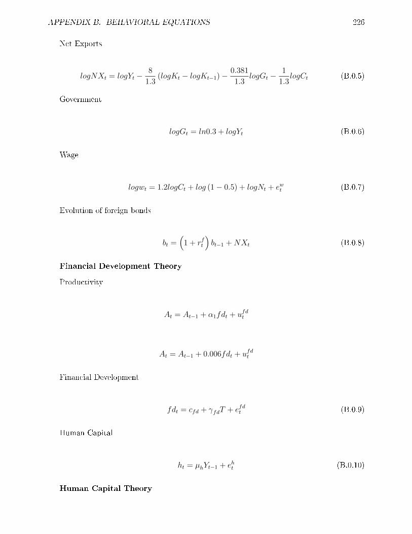
APPENDIX B. BEHAVIORAL EQUATIONS 226
Net Exports
logNXt = logYt −8
1.3(logKt − logKt−1)−
0.381
1.3logGt −
1
1.3logCt (B.0.5)
Government
logGt = ln0.3 + logYt (B.0.6)
Wage
logwt = 1.2logCt + log (1− 0.5) + logNt + ewt (B.0.7)
Evolution of foreign bonds
bt =(
1 + rft
)bt−1 +NXt (B.0.8)
Financial Development Theory
Productivity
At = At−1 + α1fdt + ufdt
At = At−1 + 0.006fdt + ufdt
Financial Development
fdt = cfd + γfdT + efdt (B.0.9)
Human Capital
ht = µhYt−1 + eht (B.0.10)
Human Capital Theory

APPENDIX B. BEHAVIORAL EQUATIONS 227
Productivity
At = At−1 + α1ht + uht
At = At−1 + 0.05ht + uht
Financial Development
fdt = µfdYt−1 + efdt (B.0.11)
Human Capital
ht = ch + γhT + eht (B.0.12)
Market Clearing Conditions Goods section
Yt = Ct + It +Gt + EXt − IMt (B.0.13)
It = Kt − (1− δ)Kt−1 (B.0.14)

Appendix C
Literature Review on Tables
Table C.1: Cross-Country Sudies
228
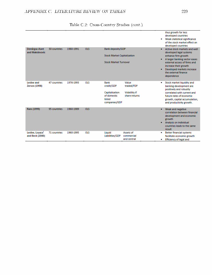
APPENDIX C. LITERATURE REVIEW ON TABLES 229
Table C.2: Cross-Country Studies (cont.)

APPENDIX C. LITERATURE REVIEW ON TABLES 230
Table C.3: Cross-Country Studies (cont.)

APPENDIX C. LITERATURE REVIEW ON TABLES 231
Table C.4: Cross-Country Studies (cont.)

APPENDIX C. LITERATURE REVIEW ON TABLES 232
Table C.5: Time-Series Studies

APPENDIX C. LITERATURE REVIEW ON TABLES 233
Table C.6: Time-Series Studies (cont.)

APPENDIX C. LITERATURE REVIEW ON TABLES 234
Table C.7: Panel Studies

APPENDIX C. LITERATURE REVIEW ON TABLES 235
Table C.8: Panel Studies (cont.)

APPENDIX C. LITERATURE REVIEW ON TABLES 236
Table C.9: Panel Studies (cont.)

APPENDIX C. LITERATURE REVIEW ON TABLES 237
Table C.10: Panel Studies

APPENDIX C. LITERATURE REVIEW ON TABLES 238
Table C.11: Country-Case Studies

APPENDIX C. LITERATURE REVIEW ON TABLES 239
Table C.12: Country Case Studies (cont.)
Table C.13: Country Case Studies (cont.)