Financial Econometrics

MFE MATLAB Introduction

Kevin SheppardUniversity of Oxford

www.kevinsheppard.com

September 2019

©2019 Kevin Sheppard

Contents

Installation and Setup i

1 Getting Started 1

2 Basic Input and Operators 5

3 Functions 9

4 Accessing Elements in Matrices 13

5 Program Flow 15

6 Logical Operators 17

7 Importing Data into MATLAB 19

8 Tables 21

9 Graphics 23

Installation and Setup

This section covers information relevant to getting up and running with MATLAB.

Installing MATLAB

MATLAB is available to install on your local PC or Mac. An overview of the process to download MATLAB

is available at

http://www.eng.ox.ac.uk/∼labejp/TAH/matlabTAH.html

and specific instructions are available at

http://www.eng.ox.ac.uk/∼labejp/TAH/MATLAB_Install.pdf

You will need your single sign-on name in order to download MATLAB. You will also require the MFE

toolbox during the course, which is available at available at

http://www.kevinsheppard.com/MFE_Toolbox

The toolbox can be installed using the function addToPathwhich you will find after unzipping the files on

your hard drive. Finally, in order to complete the tutorial on your own PC, you will need the zipped data

files available at

https://www.kevinsheppard.com/MFE_MATLAB

Some help for installing MATLAB on your computer is available at

http://www.eng.ox.ac.uk/∼labejp/TAH/TAH_Trouble_Shooting.pdf

Add the MFE Toolbox to the Path

Extract the contents of the MFE toolbox somewhere on your computer and then use the GUI tool located

under File>Set Path... to add these directories to your MATLAB path.

To verify that you were successful, close and reopen MATLAB, the run the following command

which acf -all

The output should be

PATH\WHERE\YOU\PUT\THE\TOOLBOX\timeseries\acf.m

i

If you see ’acf’not found. something has gone wrong.1

If you get an error about not being able to save the path, enter edit startup.m in the command window,

and then type the following into the editor window

pd = pwd

cd PATH\WHERE\YOU\PUT\THE\TOOLBOX\

addToPath -silent

cd(pd)

This will add the MFE toolbox to your path each time you open MATLAB.

1PATH\WHERE\YOU\PUT\THE\TOOLBOX\ is the location where you extracted the files. For example, on Windows, it may besomething likeC:\users\username\documents\MFEToolbox\or on OSX it might be/Users/username/MFEToolbox/.

ii

Lesson 1

Getting Started

This lesson covers:

• Launching MATLAB

• Launching the editor

• Creating a startup file

Launching MATLAB

To launch MATLAB, select Start>Programs>MATLAB>R2017b>MATLAB R2017b.1 When MATLAB opens, a

window similar to figure 1 should be present, although the contents of the panes may vary.

Problem 1 (Launching MATLAB). Open MATLAB on your terminal.

Launch the Editor

Once MATLAB is up and running, launch the editor. There are two methods to accomplish this task

• Enter edit in the command window

• Use the menu via File>New>M-File.

The editor should appear similar to figure 1.2.

Problem 2 (Launch the Editor). Open the editor using one the methods above. Once the editor is open,

create a file with the following contents:

x = exp(1)

y = log(x)

and save it as lesson1.m. Go to the command window and enter lesson1. The command window should

show

x = 2.7183

y = 1

1The version may be different depending on what the Mathworks is distributing.

1

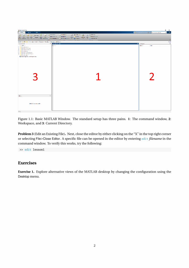
Figure 1.1: Basic MATLAB Window. The standard setup has three pains. 1: The command window, 2:Workspace, and 3: Current Directory.

Problem 3 (Edit an Existing File). Next, close the editor by either clicking on the “X” in the top right corner

or selecting File>Close Editor. A specific file can be opened in the editor by entering edit filename in the

command window. To verify this works, try the following:

>> edit lesson1

Exercises

Exercise 1. Explore alternative views of the MATLAB desktop by changing the configuration using the

Desktop menu.

2

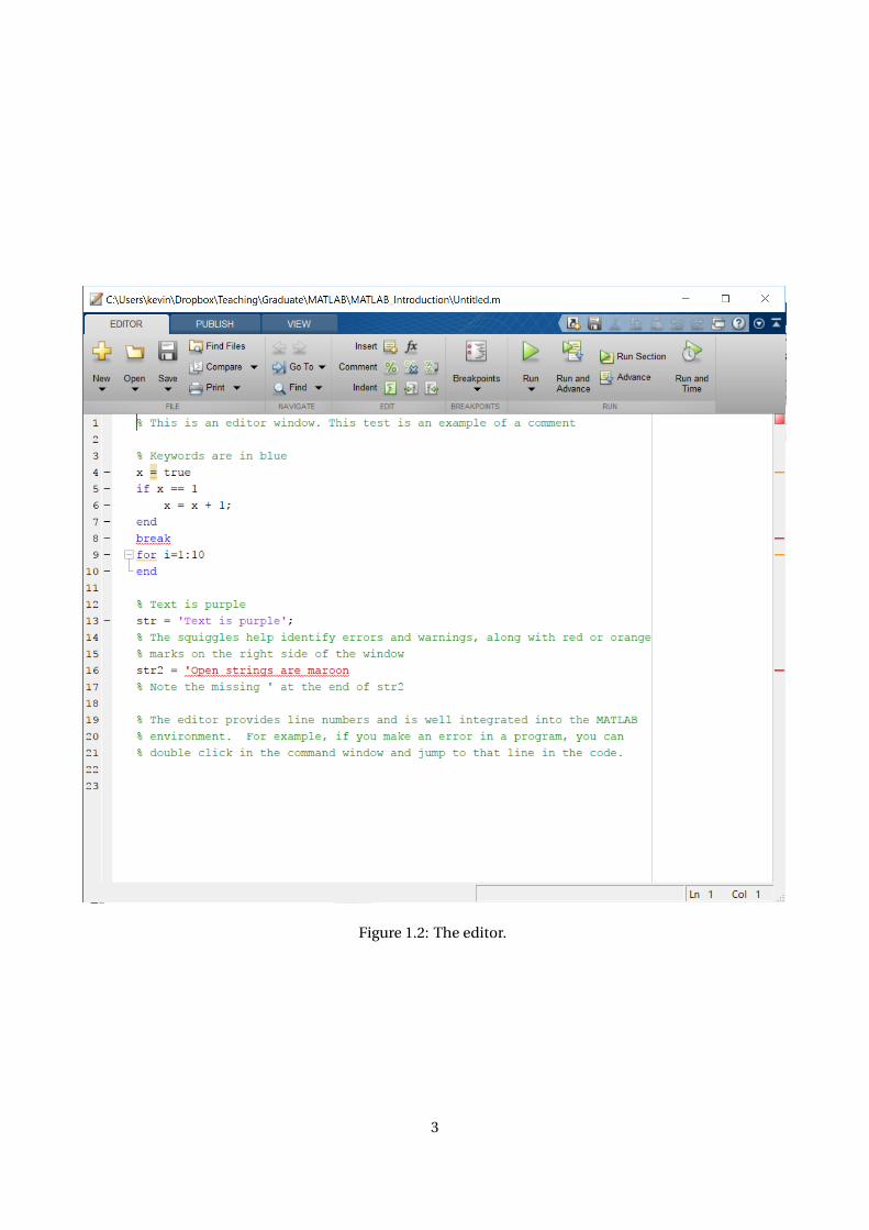
Figure 1.2: The editor.

3

4

Lesson 2

Basic Input and Operators

This lesson covers:

• Manually inputting data in scalars, vectors and matrices

• Basic mathematical operations

• Saving and loading data

September 2018 prices (adjusted closing prices) for the S&P 500 EFT (SPY), Apple (AAPL) and Google

(GOOG) are listed in table 2.1.

Problem 4 (Input scalar data). Create 3 variables, one labeled SPY, one labeled AAPL and one labeled GOOG

that contain the September 4 price of the asset. For example, to enter the Google data,

>> GOOG = 1197.00

GOOG =

1197.00

Problem 5 (Semicolon (;)). Re-enter the data in the previous task but this time use a semicolon (;) to

suppress output. Verify that the value is correct by entering the ticker symbol alone on the command

prompt (and without a semicolon). For example,

>> GOOG = 1197.00;

>> GOOG

GOOG =

1197.00

Problem 6 (Input a Row Vector). Create row vectors for each of the days in Table 2.1 named SepXX where

XX is the numeric date. For example,

>> Sep04 = [289.81 228.36 1197.00];

Problem 7 (Input a Column Vector). Create column vectors for each of the ticker symbols in Table 2.1

named SPY, AAPL and GOOG, respectively. For example,

5

Prices in September 2018

Date SPY Price AAPL Price GOOG Price

Sept 4 289.81 228.36 1197.00Sept 5 289.03 226.87 1186.48Sept 6 288.16 223.10 1171.44Sept 7 287.60 221.30 1164.83Sept 10 288.10 218.33 1164.64Sept 11 289.05 223.85 1177.36Sept 12 289.12 221.07 1162.82Sept 13 290.83 226.41 1175.33Sept 14 290.88 223.84 1172.53Sept 17 289.34 217.88 1156.05Sept 18 290.91 218.24 1161.22Sept 19 291.44 216.64 1158.78

Table 2.1: S&P 500 SPDR (SPY), Apple (AAPL) and Google (GOOG) price data in 2018.

>> GOOG = [1197.00;1186.48;1171.44;1164.83;1164.64;1177.36;

1162.82;1175.33;1172.53;1156.05;1161.22;1158.78];

Problem 8 (Input a Matrix). Create a matrix named prices containing Table 2.1. A matrix is just a column

vector containing row vectors. For example,the first two days worth of data are

>> prices = [289.81 228.36 1197.00; 289.03 226.87 1186.48];

Problem 9 (Construct a Matrix from Row and Column Data). Create a second matrix named pricesrow

from the row vectors previously entered such that the results are identical to returns. For example, the

first two days worth of data are

>> pricessrow = [Sep04;Sep05];

Create a third matrix named pricescol from the 3 column vectors entered such that the results are iden-

tical to prices

>> pricescol = [SPY APPL GOOG];

Verify that all three matrices are identical by entering

>> pricescol - prices

>> pricesrow - prices

and that all elements are 0.

Problem 10 (Saving Data). Save all data to a file named myfirstmat. Next save only the returns matrix,

prices, to a file named pricesonly.

>> save myfirstmat

>> save pricesonly prices

Verify that your data was saved by clearing all variables using

6

>> clear all

and then loading the files using the load command.

Problem 11 (Addition and Subtraction). Add the prices of the three series together. Add the prices in

Sep04 to the prices of GOOG. What happens?

Problem 12 (Multiplication). Multiply the price of Google by 2.

Problem 13 (Constructing portfolio returns). Set up a vector or portfolio weights

w =(

1

3,

1

3,

1

3

)and compute the price of a portfolio with 1 share of each.

Note: Division uses the slash operator (/).

Problem 14 (Compute returns). Compute returns using

>> returns = diff(log(prices))

which computes the first difference of the natural log of the prices. Mathematically this is

rt = ln (Pt )− ln (Pt−1) = ln

(Pt

Pt−1

)≈ Pt

Pt−1− 1.

Additionally, extract returns for each name using

>> SPYr = returns(:,1);

>> AAPLr = returns(:,2);

>> GOOGr = returns(:,3);

Problem 15 (Mean, Standard Deviation and Correlation). Using the function mean, compute the mean of

the three returns series one at a time. For example

>> GOOGmean = mean(GOOGr)

Next, compute the mean of the matrix of returns using

>> retmean = mean(returns)

What is the relationship between these two? Repeat this exercise for the standard deviation (std). Finally,

compute the correlation of the matrix of returns (corr).

Problem 16 (Summing all elements). Compute the sum of the columns of returns. How is this related to

the mean computed in the previous step?

Problem 17 (Maximum and Minimum Values). Compute the minimum and maximum values of the columns

of returns using the min and max commands.

Problem 18 (Rounding Up, Down and to the Closest Integer). Rounding up is handled by ceil, round-

ing down is handled by floor and rounding to the closest integer is handled by round. Try all of these

commands on 100 times returns. For example,

7

>> round(100*returns)

Problem 19 (Element-by-Element Multiplication). Mathematical commands in MATLAB obey the rules

of matrix algebra. This is why the portfolio returns could be easily computed as above. MATLAB also

supports element-by-element operations using the “dot” operations, .* (multiplication) and ./ (division).

Multiply the returns of Google and SPY together using the dot operator.

Problem 20 (Save the Data). Save the data created in this step using save to a file called stock-prices.mat.

You should save Google, AAPL, SPY and returns and pricescol.

8

Lesson 3

Functions

This lesson covers:

• Calling function with more than one input and output

• Calling functions when some inputs are not used

• Writing a custom function

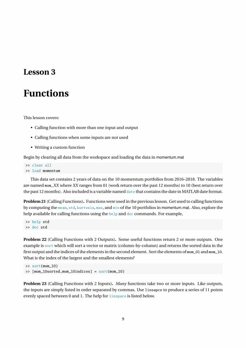
Begin by clearing all data from the workspace and loading the data in momentum.mat

>> clear all

>> load momentum

This data set contains 2 years of data on the 10 momentum portfolios from 2016–2018. The variables

are named mom_XX where XX ranges from 01 (work return over the past 12 months) to 10 (best return over

the past 12 months). Also included is a variable named date that contains the date in MATLAB date format.

Problem 21 (Calling Functions). Functions were used in the previous lesson. Get used to calling functions

by computing the mean, std, kurtosis, max, and min of the 10 portfolios in momentum.mat. Also, explore the

help available for calling functions using the help and doc commands. For example,

>> help std

>> doc std

Problem 22 (Calling Functions with 2 Outputs). Some useful functions return 2 or more outputs. One

example is sort which will sort a vector or matrix (column-by-column) and returns the sorted data in the

first output and the indices of the elements in the second element. Sort the elements of mom_01 and mom_10.

What is the index of the largest and the smallest elements?

>> sort(mom_10)

>> [mom_10sorted,mom_10indices] = sort(mom_10)

Problem 23 (Calling Functions with 2 Inputs). Many functions take two or more inputs. Like outputs,

the inputs are simply listed in order separated by commas. Use linsapce to produce a series of 11 points

evenly spaced between 0 and 1. The help for linspace is listed below.

9

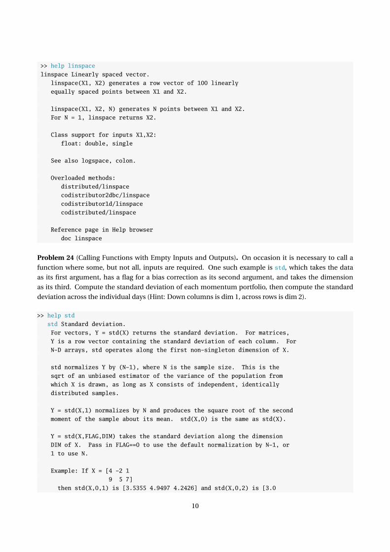
>> help linspace

linspace Linearly spaced vector.

linspace(X1, X2) generates a row vector of 100 linearly

equally spaced points between X1 and X2.

linspace(X1, X2, N) generates N points between X1 and X2.

For N = 1, linspace returns X2.

Class support for inputs X1,X2:

float: double, single

See also logspace, colon.

Overloaded methods:

distributed/linspace

codistributor2dbc/linspace

codistributor1d/linspace

codistributed/linspace

Reference page in Help browser

doc linspace

Problem 24 (Calling Functions with Empty Inputs and Outputs). On occasion it is necessary to call a

function where some, but not all, inputs are required. One such example is std, which takes the data

as its first argument, has a flag for a bias correction as its second argument, and takes the dimension

as its third. Compute the standard deviation of each momentum portfolio, then compute the standard

deviation across the individual days (Hint: Down columns is dim 1, across rows is dim 2).

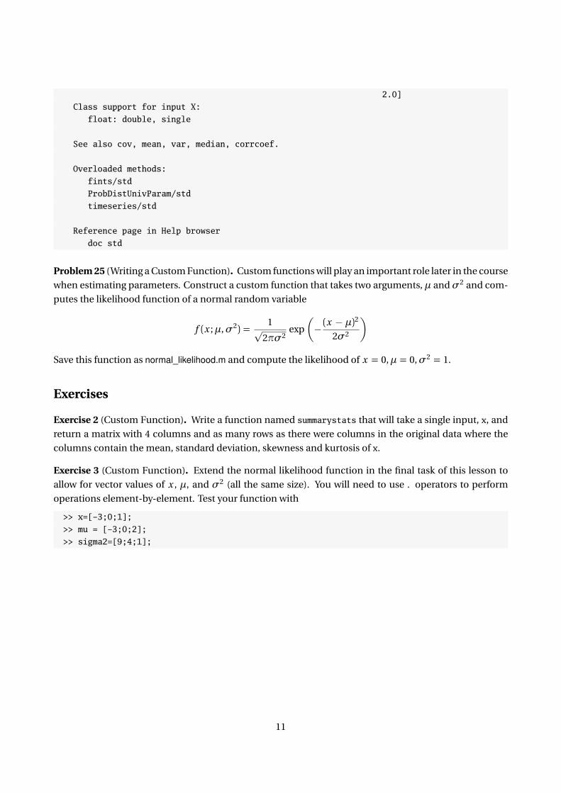
>> help std

std Standard deviation.

For vectors, Y = std(X) returns the standard deviation. For matrices,

Y is a row vector containing the standard deviation of each column. For

N-D arrays, std operates along the first non-singleton dimension of X.

std normalizes Y by (N-1), where N is the sample size. This is the

sqrt of an unbiased estimator of the variance of the population from

which X is drawn, as long as X consists of independent, identically

distributed samples.

Y = std(X,1) normalizes by N and produces the square root of the second

moment of the sample about its mean. std(X,0) is the same as std(X).

Y = std(X,FLAG,DIM) takes the standard deviation along the dimension

DIM of X. Pass in FLAG==0 to use the default normalization by N-1, or

1 to use N.

Example: If X = [4 -2 1

9 5 7]

then std(X,0,1) is [3.5355 4.9497 4.2426] and std(X,0,2) is [3.0

10

2.0]

Class support for input X:

float: double, single

See also cov, mean, var, median, corrcoef.

Overloaded methods:

fints/std

ProbDistUnivParam/std

timeseries/std

Reference page in Help browser

doc std

Problem 25 (Writing a Custom Function). Custom functions will play an important role later in the course

when estimating parameters. Construct a custom function that takes two arguments, µ andσ2 and com-

putes the likelihood function of a normal random variable

f (x ;µ,σ2) =1√

2πσ2exp

(− (x − µ)

2

2σ2

)Save this function as normal_likelihood.m and compute the likelihood of x = 0,µ = 0,σ2 = 1.

Exercises

Exercise 2 (Custom Function). Write a function named summarystats that will take a single input, x, and

return a matrix with 4 columns and as many rows as there were columns in the original data where the

columns contain the mean, standard deviation, skewness and kurtosis of x.

Exercise 3 (Custom Function). Extend the normal likelihood function in the final task of this lesson to

allow for vector values of x , µ, and σ2 (all the same size). You will need to use . operators to perform

operations element-by-element. Test your function with

>> x=[-3;0;1];

>> mu = [-3;0;2];

>> sigma2=[9;4;1];

11

12

Lesson 4

Accessing Elements in Matrices

This lesson covers:

• Accessing specific elements in vectors and matrices

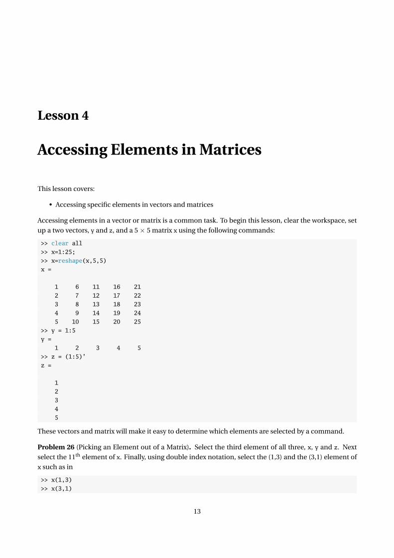
Accessing elements in a vector or matrix is a common task. To begin this lesson, clear the workspace, set

up a two vectors, y and z, and a 5× 5 matrix x using the following commands:

>> clear all

>> x=1:25;

>> x=reshape(x,5,5)

x =

1 6 11 16 21

2 7 12 17 22

3 8 13 18 23

4 9 14 19 24

5 10 15 20 25

>> y = 1:5

y =

1 2 3 4 5

>> z = (1:5)’

z =

1

2

3

4

5

These vectors and matrix will make it easy to determine which elements are selected by a command.

Problem 26 (Picking an Element out of a Matrix). Select the third element of all three, x, y and z. Next

select the 11th element of x. Finally, using double index notation, select the (1,3) and the (3,1) element of

x such as in

>> x(1,3)

>> x(3,1)

13

Which index is rows and which index is columns? Does MATLAB count across first then down or down

first then across?

Problem 27 (Selecting Entire Rows). Select the 2nd row of x using the colon (:) operator. Select the 2nd

column of z then y using the same syntax. What happens?

Problem 28 (Selecting Entire Columns). Select the 2nd column of x using the colon (:) operator.

Problem 29 (Selecting Specific Rows or Columns). Select the 2nd and 3rd columns of x using the colon (:)

operator. Select the 2nd and 4th rows of x. How can these be combined to select columns 2 and 3 and rows

2 and 4?

Exercises

Exercise 4 (Selecting Data by Date). Load the data in momentum.mat and construct a matrix containing all

of the vectors. How can all returns on a particular day be selected? How can all returns for a particular

portfolio be selected?

14

Lesson 5

Program Flow

This lesson covers:

• for loops

• Nested loops

Problem 30 (Basic For Loops). Construct a for loop to sum the numbers between 1 and N for any N . A

for loop that does nothing can be written

N = 10;

for i=1:N

end

Problem 31 (Compute a compound return). The compound return on a bond that pays interest annually

at rate r is given by

c rt =T∏

i=1

(1 + r ) = (1 + r )T

Use a for loop compute the total return for £100 invested today for 1,2,. . .,10 years. Store this variable in a

10 by 1 vector cr.

Problem 32 (Simulate a random walk). (Pseudo) Normal random variables can be simulated using the

command randn(N ,M ) where N and M are the dimensions of the desired random numbers. Simulate

100 normals in a 100 by 1 vector and name the result e. Initialize a vector p containing zeros using the

function zeros. Add the 1st element of e to the first element of p. Use a for loop to simulate a process

yi = yi−1 + ei

When finished plot the results using

>> plot(y)

Problem 33 (Nested Loops). Begin by clearing the workspace and loading momentum.mat. Begin by adding

1 to the returns to produce gross returns.1 Use two loops to loop both across time and across the 10 port-

folios to compute the total compound return. For example, if only interested in a single series, this

1A gross return is the total the value in the current period of £1 invested in the previous period. A net return subtracts theoriginal investment to produce the net gain or loss.

15

cr=zeros(size(mom_01));

gr = 1 + mom_01;

cr(1) = 1+mom_01(1);

T=10;

for t=2:T

cr(t)=cr(t-1)*gr(t);

end

would compute the cumulative return. When finished, plot the cumulative returns using plot(cr). After

finishing this assignment, have a look at doc cumsum and doc cumprod.

Exercises

Exercise 5. Simulate a 1000 by 10 matrix consisting of 10 standard random walks using both nested loops

and cumsum. Plot the results. If you rerun the code, do the results change? Why?

16

Lesson 6

Logical Operators

This lesson covers:

• Basic logical operators

• Compound operators

• Mixing logic and loops

• all and any

Begin by clearing all data and loading the data in momentum.mat

Problem 34 (Basic Logical Statements). For portfolio 1 and portfolio 10, count the number of elements

that are < 0,≥ 0 and exactly equal to 0. Next count the number of times that the returns in portfolio 5 are

greater, in absolute value, that 2 times the standard deviation of the returns in that portfolio.

Problem 35 (Compound Statements). Count the number of times that the returns in both portfolio 1 and

portfolio 10 are negative. Next count the number of times that the returns in portfolios 1 and 10 are both

greater, in absolute value, that 2 times their respective standard deviations.

Problem 36 (Logical Statements and for Loops). Use a for loop along with an if statement to simulate

an asymmetric random walk of the form

yi = yi−1 + ei + I[ei<0]ei

where I[ei<0] is known as an indicator variable that takes the value 1 if the statement in brackets is true.

Plot y .

Problem 37 (Selecting Elements using Logical Statements). For portfolio 1 and portfolio 10, select the

elements that are < 0,≥ 0 and exactly equal to 0. Next select the elements where both portfolios are less

than 0.

Problem 38 (Using find). Use find to select the index of the elements in portfolio 5 that are negative.

Next, use the find command in its two output form to determine which elements of the portfolio return

matrix are less than -2%.

17

Problem 39 (Combining flow control). For momentum portfolios 1 and 10, compute the length of the

runs in the series. In pseudo code,

• Start at i = 1 and define run(1) = 1

• For i in 2, ..., T , define run(i) = run(i-1) + 1 if sgn (ri ) = sgn (ri−1) else 1.

You will need to use length and zeros.

1. Compute the length longest run in the series and the index of the location of the longest run. Was it

positive or negative?

2. How many distinct runs lasted 5 or more days?

Exercises

Exercise 6 (all and any). Use all to determine the number of days where all of the portfolio returns were

negative. Use any to compute the number of days with at least 1 negative return and with no negative

returns (Hint: use negation (∼)).

18

Lesson 7

Importing Data into MATLAB

This lesson covers:

• Preparing data for import

• Importing data

• Converting dates

Begin by clearing all data from the workspace.

Problem 40 (Formatting Data in Excel for Import). Read the return data contained in excel.xlsx into MAT-

LAB into MATLAB using the Wizard and the function readtable.

Problem 41 (Importing Data). Reformat the data in excel.xlsx to be only numeric (convert dates to their

numeric values) and save the file as excel_for_import.xlsx. Import using xlsread.

Import the file created in the previous step and save the data to excel_imported.mat.

Problem 42 (Converting Dates). Convert the dates imported in the previous step using x2mdate.

Problem 43. Convert the Excel file to a CSV and import using csvread.

19

20

Lesson 8

Tables

This lesson covers:

• Importing data

• Extracting numerical data from Tables

Begin by clearing all data from the workspace and loading the saved stock data using load stock-data.

Problem 44 (Create a Table Existing Data). Construct a table using the three column variables SPY, AAPL

and GOOG that are loaded from stock-prices.mat created in an earlier problem.

Problem 45 (Add Dates to a Table). Construct a timetable with dates as the index to the table constructed

in the previous step. The dates can be created using

dates = []

for i = [4,5,6,7,10,11,12,13,14,17,18,19]

dates = [dates;datetime(2018,9,i)];

end

Problem 46 (Select Columns or Rows from a Table). Pull out AAPL from the table created in the previous

step. Pull it out as a simple numeric array and as a single column table. Pull out all data from the first 7

days of September for all three variables.

Problem 47 (Import into a Table). Import the data in to a table into a MATLAB table using the Wizard and

the file momentum.csv. Convert the table to a timetable.

Exercises

Exercise 7 (Practice). Getting data into and out of MATLAB is very important for your success in the com-

puting portion of the course. Practice on the file excel_practice.xlsx which is available on the website. This

file contains a subset of the important database provided by Ken French. You will need to manipulate it

in Excel before importing. The date column is in the form YYYYMM so this should be converted to a date

format like YYYY-MM-01 so MATLAB will recognize it. Additionally, you should rename the variables to

have valid MATLAB names.

http://www.kevinsheppard.com/wiki/MFE_MATLAB_Introduction

21

22

Lesson 9

Graphics

This lesson covers:

• Basic plotting

• Editing plots

• Subplots

• Histograms

Begin by clearing all data from the workspace and loading the data in hf.mat. This data set contains high-

frequency price for IBM and MSFT on a single day and times in MATLAB format.

Problem 48 (Basic Plotting). Plot the series labeled IBMprice which contains the price of IBM. Add a title

and label the axes. Use the interactive tool to add markers and remove the line.

Problem 49 (Subplot). Create a 2 by 1 subplot with the price of IBM in the top subplot and the price of

MSFT in the bottom subplot.

Problem 50 (Plot with Dates). Plot the price of IBM against the series IBMdate. Use datetick to reformat

the x-axis.

Problem 51 (Histogram). Produce a histogram of MSFT returns (Hint: you have to produce the Microsoft

returns first).

23