FINANCIAL FRAGILITY, ASSET BUBBLES, CAPITAL STRUCTURE AND REAL

RATE OF GROWTH - A STUDY OF THE INDIAN ECONOMY DURING 1970 -2000

FINAL REPORT SUBMITTED TO THE PLANNING COMMISSION

BY INDIAN INSTITUTE OF SOCIAL WELFARE & BUSINESS MANAGEMENT,

KOLKATA

JUNE 2001

Project Director : Dr. Amitava Sarkar Indian Institute Of Social Welfare & Business Management,

Kolkata. Joint Project Director : Dr. Kalyan Kumar Roy Indian Institute Of Social Welfare & Business Management,

Kolkata. Research Faculty : Dr. Soumitra Kumar Mallick Indian Institute Of Social Welfare & Business Management,

Kolkata.

Dr. Anjan Chakrabarti Department of Economics, University of Calcutta.

Dr. Tamal Datta Chaudhuri Industrial Investment Bank of India (IIBI), Kolkata. Research Fellow : Mr. Sayak Chatterjee Indian Institute Of Social Welfare & Business Management,

Kolkata.

Table of Contents CHAPTER I Introduction 1 CHAPTER II Financial Sector– Real Sector Inter-Relationship :

A Study of Theories and Indicators with Reference to the Indian Economy

2.1. Introduction 5 2.2. Literature Survey 6 2.3. Financial and Growth Indicators 8 2.4. The Indian Financial Structure: An Empirical

Analysis 17

2.5. Conclusion 34 Appendix: Raw Data used Included as

soft copy CHAPTER III Financial Fragility in Stock Markets : Cross-

sectional Study

3.1. Introduction 35 3.2. Cross-sectional Dataset 38 3.3. The Model 58 3.4. Results of Goodness-of-Fit 61 3.5. Results of Volatility 65 3.6. Conclusion 73 Appendix: Raw Data used Included as

soft copy CHAPTER IV Financial Fragility in Stock Markets : Time Series

Study

4.1. Introduction 75 4.2. Time Series Dataset 75 4.3. Time Series Model 82 4.4. Time Series Results (Goodness-of-Fit) 86 4.5. Time Series Results (Volatility) 95 4.6. Conclusion 97 Appendix: Raw Data used Included as

soft copy CHAPTER V Financial Fragility in Stock Markets: Macro-

Monetary Policy Analysis

5.1. Introduction 98 5.2. Time Series Dataset 99 5.3. Time Series Model 108 5.4. Time Series Results (Goodness-of-Fit) 112 5.5. Time Series Results (Volatility) 121 5.6. Conclusion 123 Appendix: Raw Data used Included as

soft copy CHAPTER VI Financial Fragility in the Banking Sector : A Time

Series Analysis of Non-Performing Assets

6.1. Introduction 124 6.2. The Model 128 6.3. The Dataset 130 6.4. Time Series Results 134 6.5. Conclusion 136 Appendix: Raw Data used Included as

soft copy CHAPTER VII Conclusion

Areas of Further Research 138

Bibliography 144

1

CHAPTER I

INTRODUCTION We have long been aware of the beneficial impact of a well functioning financial infrastructure on

the real sector of the economy. Conversely, the economic turmoil in the recent East Asia crisis

have once again brought into sharp focus the key role of financial fragility in aggravating crises

through the banking, currency and securities markets in particular, hampering investor confidence

operating in such markets and thus seriously impeding the ability of securities markets in

performing the intermediary role between the savers and investors.

Given the intertwined financial and real sectors, the conduct of proper macroeconomic

management and attainment of macro-objectives is dependent in a large measure on the health –

in respect of both width and depth – of the financial system as well. The lack of this or financial

fragility has been identified as a major source in the periodic crises within the last couple of

decades and the recent East Asian Crisis in 1997 with problems in the banking sector, deepening

of the currency crisis and an almost meltdown in the stock markets, with one setting the crisis in

motion and the other exacerbating the others.

In this study, the first part (Chapter II) deals with an analysis of the intertwining of the financial

and real sectors, following the frameworks of (1) Beck, Demirgiic-Kunt and Levine (BDL), (2)

King and Levine (K-L) and (3) Rangarajan identifying the major variables and measures of the

nexus between the two. The plan of this part of the study is as follows: Section I presents the

introduction; Section II surveys the existing literature; Section III discusses the financial and

growth indicators; Section IV attempts an empirical analysis in the context of the Indian financial

structure and Section V presents the conclusion.

The next part of our study delves into a detailed empirical analysis of the stock markets, in

particular, looking into the existence of (larger than normal) deviations and their persistence over

2

time, i.e., presence of asset bubbles, and as such presents findings on extent of financial fragility

or the lack of it in the stock markets. In order to investigate the extent to which the stock markets

are linked to the fundamental variables, we look at (1) an assortment of basic financial/real

variables, e.g., net worth per share (book value per share), profit per share (EPS), dividend per

share and debt-equity ratio; (2) dynamic variables, like rate of growth of net worth per share, profit

per share, dividend per share and debt-equity ratio as surrogates for expectations; and (3)

macroeconomic policy variable, like prime lending rate. We have attempted both cross-section

and time-series analyses on (1) and (2) and a time-series analysis on (3).

The cross-sectional study (Chapter III) is discussed in six sections. Section I is the introduction.

Section II discusses the dataset; Section III discusses the model; Section IV analyses the results

of goodness-of–fit; Section V analyses the results of volatility and Section VI presents the

conclusion.

The time-series study (Chapter IV) is discussed in six sections. Section I is the introduction.

Section II discusses the dataset; Section III discusses the model; Section IV analyses the results

of goodness-of–fit; Section V analyses the results of volatility and Section VI presents the

conclusion.

The macro-monetary policy analysis (Chapter V) is discussed in six sections. Section I is the

introduction. Section II discusses the dataset; Section III discusses the time-series model; Section

IV analyses the results of goodness-of–fit; Section V analyses the results of volatility and Section

VI presents the conclusion.

The sources of financial fragility can be traced, among others, in the banking, currency and asset

markets as has been mentioned earlier. Solvency of banks may be threatened by the factors

operating at both the global and national levels. The existing literature ( Allen and Gayle (2000),

Kaminsky and Reinhart (1999, 1996), Kiyotaki and Moore (1997), Rakshit (1998), Stiglitz (1981))

3

has expressed concern over the inherent tendencies in the banking sector towards fragility,

arising out of institutional characteristics with respect to norms / rules and inadequate controls.

Further, our study and empirical analysis brings out three significant tendencies. First, NPAs (as a

ratio of loans and advances) are significantly sticky over time. Second, larger NPAs are

associated with larger advances and vice-versa; and third, NPAs do not seem to be spiraling out

of control, rather shows signs of a slight reduction. The policy initiated during the 90s of

classifying bad debts as NPAs after two installment defaults, seems to have brought some

amount of control on the bad debts situation.

With the collapse of the Bretton-Woods fixed exchange rate system and introduction of freely

floating exchange rates from 1973 practically by all industrialised countries, it was observed that

exchange rates exhibited considerable volatility, prolonged periods of overvaluation and

undervaluation in both size and duration, all indicating currency markets not being satisfactorily

determined by fundamentals leading to financial fragility in such markets, thus, further

compounding the task of macroeconomic management in general and balance of payments

adjustment in particular.

In case of India, the switch to a floating exchange rate regime (at least on current account) from

the prior multi-currency peg (adopted in 1975) was accomplished gradually between 1991-93.

There was significant variability in the rupee exchange rate vis-à-vis major currencies like the

U.S. dollar. Further and more importantly, when we look at the exchange rate movements and

their relationship with fundamental variables, like the price level, with the theory of purchasing

power parity (PPP), for example, it provides the theoretical basis of the belief that changing

exchange rate under floating system would offset inflation differentials. However, particularly after

1993 given the increased flexibility of the exchange rate regime, when nominal exchange rate

movements are expected to reflect changes in the price levels, we consistently find the exchange

rate movements to exceed the changes in price levels, suggesting exchange rate movements in

4

currency markets not being adequately explained by fundamental explanatory variables like

relative inflation rates.

In the limited scope of our present investigation, we have not attempted to study the impact of the

currency markets on financial fragility, though a preliminary study of the health of the banking

sector, namely (1) a brief review of the institutional and almost endemic fragility in the banking

industry and (2) some areas of specific concerns, particularly in respect of the NPAs have been

attempted. Section I is the introduction. Section II discusses the model; Section III discusses the

dataset; Section IV analyses the time-series results; and Section V presents the conclusion.

Our framework of research identifies a functional (i.e. fundamentals based) analysis of the extent

of fragility in the banking sector and the currency markets as areas for further research.

5

CHAPTER II

Financial Sector-Real Sector Inter-relationship: A Study of Theories and Indicators with Reference to the Indian Economy

2.1 INTRODUCTION In this chapter, we intend to study the importance of financial sector development and its relationship with

the real variables and their growth. It is only in very recent times that economists are beginning to believe in

this linkage. For a long time, notwithstanding the influence of Phillips curve in between (whose long run

effect was anyway found to be ineffective), economists in the Walrasian tradition have trenchantly believed

in the classical dichotomy: financial sector does not matter for real sector development and its growth. Still,

a large segment of economists believe strongly in that tradition (the real business cycle school, for

example). However, the Walrasian framework is built on the critical assumption that all markets clear. In

recent times economists have challenged this assumption and subsequently adopted capital market

imperfection as their point of departure. Using this new framework, they demonstrate that financial sector

development matters for the development of the real sector and is growth-enhancing.

We will begin this chapter by reviewing the literature in substantial details explaining the basic ideas of the

models that seek to demonstrate the relevance of financial development for the real sector. Thus one of the

central programs in this chapter is in finding out indicators pointing to the development of the financial

sector. In the next section, we will review the financial and growth indicators as developed by economists,

especially the former in the context of certain issues. These issues concern the depth of the financial

sector, activity of the financial sector, stock and bond market development, success of the financial sector

reforms and the linkage between the financial development and growth. Subsequently, in the section “The

Indian Financial Structure: An Empirical Analysis”, we intend to use some of these indicators to study the

development of the financial sector and touch on its linkage with the real sector in the context of the Indian

economy. This will give us considerable insight into the state of the Indian financial system, its depth and

6

size as well as the success of the economic reform and whether the financial development is significantly

correlated with the real sector. Finally, there will be a conclusion.

2.2 LITERATURE SURVEY

It is only in very recent times that economist started looking for indicators of financial sector that will capture

its development, structure and performance. The reason for this historical delay lies in the discomfort of

economist regarding the relation between the financial sector and the real sector as well as its growth. Till

the early 1980s there was a general absence of models that could explain the relationship between the two

sectors.

From the 1980s onward things started to change. Now there are a large section of economists who believe

that the financial sector does matter for the real variables and their growth. Their arguments as to how it

matters are also diverse but there is also a thread of similarity in all these different viewpoints. And it has to

do with credit market imperfection. Credit market imperfection makes financial intermediation matter for the

real variables.

The seminal paper to highlight the role of financial institutions in matters of investment and output was

written by Stiglitz & Weiss (1981). They pointed out that with asymmetric information and interest rate

serving as a screening device for separating out bad borrowers (with higher probability of default) from

good borrowers, credit rationing is produced. Credit rationing, by reducing the amount of available loanable

funds, produces under-investment and hence output is adversely affected. So they concluded that financial

institution matters.

Friedman and Schwartz (1963), Bernanke (1983) and Bernanke and Gertler (1989) pointed out that

fluctuations in the real variables are caused by financial dislocation. In these cases the financial

intermediation role of the bank is again critical. The model by Bernanke and Gertler has been especially

influential. It is assumed in the model that firms cannot fund their project through internal funds only. But

7

then in case of firms relying also on outside funds, the problem of asymmetric information arises for

financial institutions. This involves monitoring costs and subsequently leads to a selected number of firms

getting loans and consequently to the restriction of credit. Thus only a limited number of better projects get

funded. In such a framework, a shock to the economy may end up increasing the monitoring cost thereby

restricting credit and reducing investment. Thus financial fragility will affect the real sector.

Kiyotaki and Moore (1997) and Franklin and Gale (2000) extended the spirit of the above approach to

include the financial contagion effect. They pointed out that crisis originating in one point of the financial

sector has the capability to spread to other points thereby becoming contagion and producing a crisis of the

entire financial sector. The mechanism through which the contagion happens is some form of asset-based

claims that overlap between agents or regions or banks. Franklin and Gale (2000) showed that a banking

crisis originating in one region spreads to other regions because of the overlapping claims of banks or

regions. If a region suffers a loss then the claim on the suffering region falls in value, which if of higher

magnitude, is capable of producing a crisis in the adjoining regions. Hence crisis in one point move from

region to region becoming a contagion.

Kiyotaki and Moore (1997) showed that asset–based collaterised borrowing (especially stock market and

real estate based) has the capacity of producing extreme financial fragility with its subsequent disastrous

effect in the real sector. During boom time, asset prices shoot up and potential borrowers buy these assets

at inflated price. Now either bank give loans to the borrowers against these assets or the borrowers may

use part of the loans in buying the assets. Either way, a shock to the economy may see lenders recalling

asset based collaterised loans thereby producing extreme reductions in asset price. The bubble bursts.

Those borrowers (firms & agents) who bought assets at inflated prices default with the collapse of those

prices. Firms start closing down and banks stop lending. Thus in both Kiyotaki and Moore, and Franklin and

Gale, banks behave procyclically lending less during recession. This finding has also been supported by

Kaminsky and Reinhart (1996;1999) who looked at figures of crisis in 20 countries. They found that at times

of high expectation and growth, the asset prices rose way over the average and its expansion was to a

8

large extent supported by borrowings from banks. When the bubbles burst and the asset prices collapsed,

financial institutions with overexposure to those asset markets ran into crisis with a lag.

While the above models have significantly articulated the relationship between the financial sector and the

real sector, the problem of associating financial sector with neo-classical style growth still remained. This

was ultimately addressed by King and Levine (1993a, 1993b) who extended the endogenous growth theory

(Aghion and Howitt 1992; Romer 1990) to demonstrate that financial development is growth enhancing.

Thus economists are presently in a position to believe in certain results. Namely, that financial sector is

closely linked with real sector and that financial development is growth enhancing.

After the relationship between the financial sector and real sector as well as its growth has been secured,

the process of constructing financial indicators as well as growth indicators began. Of special interest are

the financial development indicators for revealing the extent of this development, which should tell us

something about its effect on the real sector.

2.3 FINANCIAL AND GROWTH INDICATORS

For long the International Monetary Fund’s International Financial Statistics and International Finance

Corporations have been the source of financial development indicators used by economists. But in recent

times, complementary studies on financial indicators have proliferated. Theoretical models on financial

sector have been complemented by a search by economists for indicators designed to capture the size,

activity and efficiency of the financial sector as a whole as well as specific financial markets such as the

bond and stock market. While the literature on financial indicators is by now substantial, we will focus on

three papers - Beck, Demirgiic-Kunt and Levine (2000) henceforth called BDL, King and Levine (1993)

called K-L and Rangarajan (1997). We believe that the list of indicators presented by the three papers is

comprehensive and that these three papers more or less encapsulate the development in this field thus far.

9

Depending upon the issues posed, we will be charting out the indicators as given by BDL, KL and

Rangarajan. Before we begin, let us distinguish between the groups of financial institutions as presented

by BDL. BDL divided financial institutions into three groups -- Central Bank under the control of monetary

authorities, deposit money banks comprising of financial institutions with liabilities in checkable form or

otherwise for making payments and other financial institutions such as non-bank financial institutions or of

any other type who do not incur liabilities that require payments. BDL further makes a distinction between

private credit and assets where the former refers to total claims on the private sector and the latter is

understood as the total claims on domestic non-financial sectors.

Let us now pose the issues and the financial indicators designed to address them.

Depth of the Financial Development We study the depth of the financial structure by looking at the financial indicators measuring the relative

importance of the three financial groups and that measuring the size of financial structure relative to GDP.

10

Relative Size Measures

Rangarajan B-D-L K-L Central Bank Assets Total Financial Assets Deposit Money Bank Assets Total Financial Assets Other Financial Institution’s Assets Total Financial Assets

Intermediation Ratio = Secondary Issue Total Issue Or Proportion of claims issued to financial institutions to the issues of non-financial sectors.

Alternative Measure

Deposit Money Bank Assets Central Bank Assets + Deposit Money Bank Assets

Deposit Money Bank Domestic Assets BANK = Deposit Money Bank Domestic Assets + Central Bank Domestic Assets

The only point to note here is that of the alternative measure of finding the relative size of the financial

groups mentioned by BDL. BDL points out that the first three indicators may not be available. In that case,

it is useful to use the alternative measures that captures the relative size of deposit money bank assets to

the central bank. This alternative measure is the same as BANK used by K-L. Increase in BANK means

more financial services and higher levels of financial development.

Absolute Size Indicators

Rangarajan B-D-L K-L Financial

Liquid Liabilities

DEPTH = Liquid Liabilities GDP Liquid Liabilities = Currency held outside of the

11

Ratio=Total Financial Issues GDP

GDP Liquid Liabilities = Same as in K-L

banking system + demand and interest bearing liabilities of banks and non bank financial intermediaries

In this case increase in DEPTH will indicate an increase in the depth of financial

development and growing role of financial intermediaries.

Activity of the Financial Intermediaries

The focus is on the financial intermediaries’ claims on the private sector. The set of indicators is designed to

capture the role of financial sector in allocating credit.

Rangarajan B-D-L K-L Financial interrelationship = Increase in the stock of financial claims Net capital formation

Private Credit by deposit money banks GDP Private Credit by deposit money banks and other financial institutions GDP

PR1V = Credit issued to private enterprises GDP PRIVATE = Credit issued to private enterprises Credit issued to central and local government + credit issued to private and public enterprises

Increases in these indicators mean that the non-central bank intermediaries are playing an increasingly

important role in allocating credit to the non-government and non-public enterprises. And it is assumed here

that financial services is more productivity enhancing in case of the financial sector reform with the private

sector than in its interaction with the public sector.

Efficiency Measure of the Financial Sector

12

DBL consider net interest margin as a measure of the efficiency – competitiveness of the financial sector.

Declining net interest margin points to the functional level efficiency of the commercial banks and the

movement towards the market price.

Stock Market Development

The indicators as used by DBL suffice in capturing the size, activity and efficiency of the stock market.

Size of the stock Market

Stock Market Capitalization = Value of Listed Shares

GDP GDP

Increase in the ratio will indicate an increase in the size of the stock market vis-à-vis the rest of the

economy.

Activity of the stock market

Stock Market Total Value Traded

GDP

This indicator measures the degree of liquidity provided by the stock market to the economy. Efficiency of the stock market

Stock Market Turnover ratio = Value of Total Shares Traded

13

Market Capitalization

This is a measure of the liquidity of the stock market relative to its size. Higher turnover ratio means an

active stock market.

Bond Market Development We want to capture the size of the private and public bonds relative to the economy. The two together will

capture the size of the domestic bond market. The two ratios then are

Private Bond Market Capitalization GDP and,

Public Bond Market Capitalization GDP Success of the Financial Sector Reform We divide the time period between the pre-reform and the post-reform period. Then changes in indicators

as indicated in the direction below will capture the success or failure of reform. We lump together the

indicators as put forward by BDL, K-L and Rangarajan.

Success of Reforms

Financial Development Indicators

↑

↑

↑

BANK

PRIVATE

PRIV/Y

14

↑

↓

↑

↑

↑

↑

↑

↑

DEPTH

CURRENCY = Currency held outside of banks Bank Deposits

REAL RATE = Real Interest Rate

Finance Ratio

Intermediation Ratio

Financial Interrelations

Stock Market Capitalization GDP

Stock Market Total Value traded GDP

Relations of Financial Development with Real Variables Here we take off from K-L who were the first to articulate a possible relationship between financial

development and economic growth. They took financial and growth indicators and then found the

correlation between the two. A strong correlation would indicate a close relationship between financial

development and economic growth. While we have already studied the financial indicators, K-L constructed

a few growth indicators.

The first growth indicator is akin to the Solow residual with the assumption that it mostly captured

productivity growth. K-L takes the aggregate production function:

Y = κ∝ x

where Y = Real per capita GDP

k = Real per capita physical capital stock

x = Other determinants of per capita growth

15

α = Production function parameter.

Taking log of the production function and differentiating, we get

x

x

k

k

y

y ���+=α

⇒ GYP = α GK + PROD ⇒ PROD = α GK – GYP

Where = y

y�GYP = Growth rate of real per capita GDP

k

k�= GK = Growth rate of the real per capita physical capital stock

x

x�= PROD = Growth rate of everything else

Once we know GYP and GK, and specifying α, we can find out PROD. As we have already pointed out,

PROD is assumed to capture productivity growth.

K-L also takes a measure of physical capital accumulation, which they call INV.

INV= Gross Domestic Investment

GDP

We are now in a position to chart out the growth indicators and the already derived financial indicators.

Growth Indicators Financial Indicators ala BDL, K-L and

Rangarajan GYP GK

PROD INV

Already defined and discussed before.

In this study we will check the following:

16

1) if each financial indicator is positively and significantly correlated with each growth indicators, and

2) If the financial indicators are highly correlated with one another.

If a) and b) holds then we say that financial development is strongly linked to economic growth.

To conclude, in this section we have built a general framework for measuring the extent

of financial sector development and its relationship with the real sector growth. In the

subsequent section, using BDL measures (which is quite comprehensive) we will mainly

concentrate on the extent of financial sector development in India. While inability to

access the data on growth in time (this itself is huge task which we hope would be done

elsewhere using the methodology presented here) is a handicap, we will construct two

alternative indicators of credit allocation to reveal whether the Indian real sector

(represented essentially by the private sector) is making use of the financial sector

development in India.

2.4 THE INDIAN FINANCIAL STRUCTURE: AN EMPIRICAL ANALYSIS

We will use the set of indicators, developed earlier in this chapter, to study the size, activity and efficiency of

financial intermediaries in India. We will also look at indicators that measure the stock and bond markets to

reveal the extent of its size, growth and efficiency. The focus of this chapter is to explore the extent of

financial development in India. The sources used for the study are CMIE Monthly bulletins, RBI – Annual

Reports, Report on Currency & Finance and Handbook of Statistics on Indian Economy for the respective

years.

17

The findings are fairly unambiguous. Firstly, there is a steady deepening of the financial development in

India. Indicators of financial intermediaries – measuring its size, growth and activity – all point to this

deepening process. Secondly, there are clear indications that non-banking sector has grown faster than

banking sector. This is also supported by clear indication about the diminishing role of RBI as a player in

the financial markets even as its role as a regulator has increased.

Thirdly, while the results unambiguously point to a deepening of the financial development in India, the

question remains as to the allocation of credit. For that, we take indicators of credit portfolio allocation and

show that the allocation of credit to government sector relative to private sector is increasing. This should

indeed be considered disturbing to planners since one of the central aims of liberalization was to achieve

the reverse. But results show that, in vying for investment, the government sector have outsmarted the

private sector.

Size and Activity of the Financial Sector in India

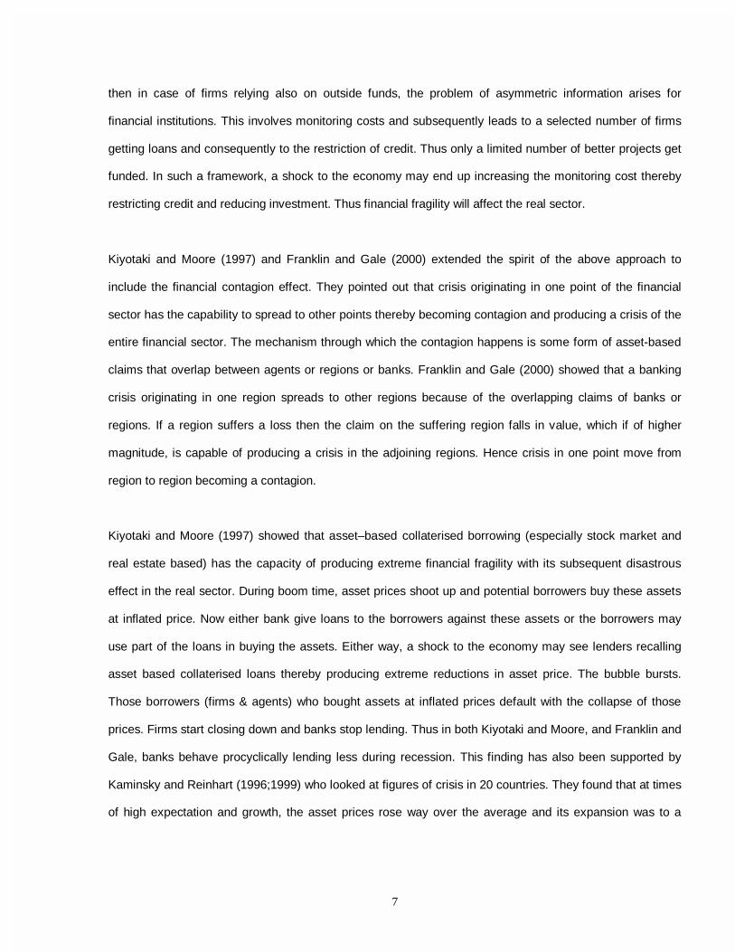
The relative size indicators measure the importance of three broadest segments of the financial sector

(defined in section II) relative to each other. These are the ratio of central bank assets to total financial

assets, ratio of deposit money bank assets to total financial assets and the ratio of other financial

institutions’ assets to total financial assets, where total financial assets are the sum of the assets of central

bank, deposit money banks and other financial institutions. As figure 1 shows, the time series movement in

the ratio of central bank assets to total financial assets shows a very interesting feature; it is gradually

decreasing since the last decade. It is also clear from the diagram that the rate of decrease is faster in the

post liberalization era. If one looks at the asset side of the RBI, it can be observed that it comprises

primarily of foreign exchange assets and credit given to the banking sector and the government. The

decline in the above ratio indicates the reduction in direct credit by RBI to the government sector and the

efficacy of replacement of the ad hoc T-Bills system by Ways and Means Advances. This ratio increased in

1998-99 and is indicative of improvement in the forex reserves position through Resurgent India Bonds.

This also indicates the move away by the RBI from that of a player to the regulatory body.

18

Yearly movement of ratio of deposit money bank assets to total financial assets (figure 2) is showing a

mixed result. After a reasonable fall during 1991-95 it is now in a slightly increasing trend. If we observe the

time series movement of the ratio of other financial institutions’ assets to total financial assets (figure 3) it is

very clear that the extent of financial disintermediation is much more dispersed in total asset creation. We

can notice a significant jump just after liberalization and it was increasing till 1997-98. After that it is slightly

decreasing which is indicative of the inactivity in the equity market. A lot of projects that were conceived and

funded by DFIs, which had an equity component, could not access the market for equity and either had to

be abandoned or equity had to be replaced by high cost debt thereby adversely affecting the financial

viability of the projects.

Fig 1. RATIO OF CENTRAL BANK ASSETS TO TOTAL FINANCIAL ASSETS

0

0.1

0.2

0.3

1980

-81

1981

-82

1982

-83

1983

-84

1984

-85

1985

-86

1986

-87

1987

-88

1988

-89

1989

-90

1990

-91

1991

-92

1992

-93

1993

-94

1994

-95

1995

-96

1996

-97

1997

-98

1998

-99

1999

-200

0

19

Fig 2. RATIO OF DEPOSIT MONEY BANK ASSETS TO TOTAL FINANCIAL ASSETS

0

0.2

0.4

0.6

0.8

1980

-81

1982

-83

1984

-85

1986

-87

1988

-89

1990

-91

1992

-93

1994

-95

1996

-97

1998

-99

20

The alternative measure captured in figure 4, which is defined as ratio of deposit money bank assets to

central bank and deposit money bank assets leads to the same conclusion that the central bank is gradually

Fig 3. RATIO OF OTHER FINANCIAL INSTITUTIONS' ASSETS TO TOTAL ASSETS

0

0.1

0.2

0.3

0.4

0.5

1980

-81

1982

-83

1984

-85

1986

-87

1988

-89

1990

-91

1992

-93

1994

-95

1996

-97

1998

-99

Fig 4. RATIO OF DEPOSIT MONEY BANK ASSETS TO CENTRAL BANK AND DEPOSIT MONEY BANK ASSETS (SINCE 1980)

0.68

0.72

0.76

0.80

0.84

0.88

1980

-81

1982

-83

1984

-85

1986

-87

1988

-89

1990

-91

1992

-93

1994

-95

1996

-97

1998

-99

21

withdrawing (not in terms of supervision) itself from being a player. But, this is a relative measurement, not

absolute one. So it is not to be understood that the total assets of central bank is decreasing year after

year.

The ratio of liquid liabilities to GDP (figure 5) is an absolute size measure based on liabilities. Liquid liability

is currency plus demand and interest bearing liabilities of banks and other financial intermediaries. The ratio

of Liquid liability (components are given in Section I) to GDP is increasing systematically during the last two

decades. Basically that implies Money Supply (M3) with respect to GDP is gradually increasing. If we

consider the relation MV=PY, where M stands for money supply during a given period, V the velocity of

circulation, P the price level for that particular period and Y physical output, then it is very clear that as M/Y

is increasing, P/V has to increase to maintain the equality. This indicator determines the depth of financial

development and the growing role of financial intermediaries. This is the broadest available indicator of

financial intermediation, since it includes all the three financial sectors.

The ratio of central bank assets to GDP (figure 6) has shown an overall increase since 1980-81, even

though its volatility has increased significantly in the post liberalization era. It may be readily observed that

Fig 5. RATIO OF LIQUID LIABILITY TO GDP (SINCE 1980)

0.00

0.50

1.00

1.50

2.00

2.50

3.00

1980-81 1982-83 1984-85 1986-87 1988-89 1990-91 1992-93 1994-95 1996-97 1998-99

22

the ratio of deposit money bank assets to GDP (figure 7) and the ratio of other financial institutions’ assets

to GDP (figure 8) are steadily increasing throughout the period we have considered. Of special significance

is the dramatic increase in the ratio of other financial institutions’ assets to GDP in the post liberalization era

where the rate of change of this ratio peaked during 1992-94.

Fig 6. RATIO OF CENTRAL BANK ASSETS TO GDP (SINCE 1980)

0.00

0.10

0.20

0.30

0.40

0.50

0.60

1980

-81

1981

-82

1982

-83

1983

-84

1984

-85

1985

-86

1986

-87

1987

-88

1988

-89

1989

-90

1990

-91

1991

-92

1992

-93

1993

-94

1994

-95

1995

-96

1996

-97

1997

-98

1998

-99

1999

-200

0

23

Fig 7. DEPOSIT MONEY BANK ASSETS TO GDP

0

1

2

3

1980-81 1982-83 1984-85 1986-87 1988-89 1990-91 1992-93 1994-95 1996-97 1998-99

Fig 8. RATIO OF OTHER FINANCIAL INSTITUTIONS ASSETS TO GDP

0

0.5

1

1.5

2

2.5

1980

-81

1981

-82

1982

-83

1983

-84

1984

-85

1985

-86

1986

-87

1987

-88

1988

-89

1989

-90

1990

-91

1991

-92

1992

-93

1993

-94

1994

-95

1995

-96

1996

-97

1997

-98

1998

-99

24

There is another point to be observed. The ratio of deposit money bank assets to GDP and the ratio of

other financial institutions’ assets to GDP reached almost the same level in 1998-99 but the path of

reaching that position were different. Starting from a relatively lower value, the ratio of other financial

institutions’ assets to GDP has undergone a faster change after the post liberalization period as compared

to the ratio of deposit money bank assets to GDP.

The next two indicators reflect the measures of the activity of financial intermediaries and focus on

intermediary claims on the private sector. The ratio of private credit by deposit money banks to GDP (figure

9) and the ratio of private credit by deposit money banks and other financial institutions to GDP (figure 10) -

- both measures isolate credit issued to the private sector as opposed to credit issued to government and

public enterprises. They concentrate on credit issued by intermediaries other than the central bank and

measure one of the main activities of financial intermediaries, i.e., channeling savings to investors. The ratio

of private credit by deposit money banks to GDP and the ratio of private credit by deposit money banks and

other financial institutions to GDP shows an increasing trend through out the period. This indicates that the

non-central bank intermediaries are playing an increasingly important role in allocating credit to the non-

government and non-public enterprises.

Fig 9. RATIO OF PRIVATE CREDIT BY DEPOSIT MONEY BANKS TO GDP

0

0.2

0.4

0.6

0.8

1

1.2

1989-90 1992-93 1995-96 1998-99

25

We have already noticed that the ratio of other financial institutions’ assets to GDP is increasing in general.

The ratio of total assets of development banks to GDP actually measures the pace of economic

development of nation. Our diagram (figure 11) suggests that though the ratio is increasing, changes are

more significant after liberalization. But what should concern us is that after 1997-98 the rate of increase of

the ratio shows a considerable decline.

Fig 10. RATIO OF PRIVATE CREDIT BY DEPOSIT MONEY BANKS AND OTHER FINANCIAL

INSTITUTIONS TO GDP

0

2

4

1989-90 1992-93 1995-96 1998-99

Fig. 11 RATIO OF TOTAL ASSETS OF DEVELOPMENT BANKS TO GDP

0.00

0.10

0.20

0.30

0.40

0.50

0.60

1980

-81

1981

-82

1982

-83

1983

-84

1984

-85

1985

-86

1986

-87

1987

-88

1988

-89

1989

-90

1990

-91

1991

-92

1992

-93

1993

-94

1994

-95

1995

-96

1996

-97

1997

-98

1998

-99

1999

-200

0

26

Efficiency of the Financial Sector in India

Interest rate margin is an indicator of efficiency of the commercial banks. Declining net interest income

(figure 12) captures the fact that the Indian financial markets are becoming competitive. This is indicative of

the process of deregulation of interest rates reflecting movement towards market rates. The yield curve is

becoming a reality. Compartmentalisation of players in different markets and products has broken down

and players can play in all markets bringing about a reduction in interest rate across sectors. For example,

financial institutions are giving working capital loans and commercial banks are giving term loans.

Furthermore, institutions are also getting into export credit, commodity credit, etc. However, resulting from a

general industrial slowdown accompanied by inactivity in the capital market due to lack of investor

confidence, there has been also relatively less demand for credit which has kept interest rates down and

kept margins under pressure.

In an environment where accounting was on accrual basis, the thrust of the banking sector was on growth

in terms of sanctions, disbursements and asset base. Irrespective of the interest rate regime, financial

sector players were borrowing at high rates and also lending at high rates, keeping the margin constant.

Over time, with accounting on actual basis and RBI guidelines on income recognition, asset classification,

provisioning and capital adequacy, the financial sector players have come to terms with the fact that high

rates of interest is also associated with high default rates and the effective rate of return is much lower than

what the banks originally presumed. With the current income recognition norms, financial sector players

have come to realise the importance of asset quality and not size. The reduction in net interest margin

mentioned above is an indicator of the fact that with provisioning associated with non-performing assets, a

lower margin may lead to a better asset quality, a healthier balance sheet, better capital adequacy levels

and enhanced shareholder value.

27

Fig. 12 NET INTEREST INCOME(SPREAD) AS % OF TOTAL ASSETS OF SCB (SINCE 1991-92)

0

1

2

3

4

1991-92 1994-95 1997-98 2000-01

28

Stock and Bond Market Development in India

The following indices are the indicators of stock market size, activities and efficiencies. The ratio of stock

market capitalization (i.e. value of listed shares) to GDP measures the size of the stock market relative to

the size of the economy. It is a measure of financial penetration. Figure 13 indicates that the movement of

this ratio is fluctuating but the changes are not very enormous from one period to another, which indicates

that private equity participation to GDP is more or less constant. In fact the increase from 1990 has not

been that significant. In other words, the extent of penetration of the financial market has not been that

intense and is reflected in the extent of inactivity in the capital market.

The ratio of stock market total value traded to GDP measures the trading volume of the stock market as a

share of national output and reflects the degree of liquidity that stock market provides to the economy. Ratio

of total trading volume of BSE (figure 14), the largest stock exchange in India, to GDP has made a “U

shaped recovery”, touching lowest in 1995-96 and increasing thereafter.

Fig 13. PERCENTAGE OF MARKET CAPITALISATION TO GDP

0

10

20

30

40

50

60

70

1989-90 1992-93 1995-96 1998-99

29

The stock market turnover ratio is the ratio of the value of total share traded to market capitalization. It is a

measure of activity or liquidity of a stock market relative to its size. A larger but less liquid stock market will

have a lower turnover ratio than a small but active stock market. Our diagram (figure 15) on this is identical

to the ratio of stock market total value traded to GDP as the penetration ratio is a constant - touching

highest in 1991-92 and lowest in 1995-96, and showing a rapid ascent after 1995-96. It may be observed

that not only did prices increased, this was accompanied by an increase in the volume of transactions. So,

this period observed a considerable extent of activity.

Fig 14. TRADING VOLUME of BSE / GDP (%)

0

10

20

30

40

50

60

70

1989-90 1992-93 1995-96 1998-99

Fig 15. STOCK MARKET TURNOVER RATIO

0

0.2

0.4

0.6

0.8

1

1.2

1.4

1989-90 1992-93 1995-96 1998-99

30

The following indicators measure the size of primary stock market and bond market as against secondary

market trading in equity and debt. The ratio of equity issue to GDP (figure 16) is quite fluctuating and is on a

declining trend since 1991-92 whereas the ratio of debt issue to GDP (figure 17) shows a “U” shaped

recovery. So it can be noted that the debt market is growing in a systematic manner whereas the equity

market is not maintaining that kind of pace. The same picture is again reflected if we study the yearly

movement of the ratio of public sector capital issue to GDP (figure 18) and private sector capital issue to

GDP (figure 19). The yearly movement of the ratio of private sector capital issue to GDP shows a declining

trend since 1991-92 whereas the ratio of public sector capital issue to GDP is maintaining a “U” shape. This

is indicative of a growth in the capital market driven by debt issues and that too of the public sector.

Fig 16. EQUITY ISSUE / GDP (%)

0

2

4

6

8

1989-90 1992-93 1995-96 1998-99

Fig 17. DEBT ISSUE / GDP (%)

0123456

1989-90 1992-93 1995-96 1998-99

31

Fig 18. PUBLIC SECTOR CAPITAL ISSUE / GDP (%)

0

1

2

3

4

5

1989-90 1992-93 1995-96 1998-99

Fig 19. PRIVATE SECTOR CAPITAL ISSUE / GDP (%)

0

2

4

6

8

10

1989-90 1992-93 1995-96 1998-99

32

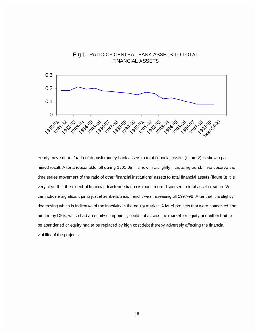
Financial Deepening and Credit Allocation in India

While financial deepening and increased efficiency did happen in India, there remains serious doubt as to

whether the private sector was able to take advantage of it. In fact, as figures 20 and 21 show, credit

portfolio has been moving in favor of government sector with the percentage of non-food credit to total

credit falling distinctly. This is in sharp contrast to the increase in percentage of investment in GOI to total

credit. In terms of investment, the government sector seems to be catching up with the private sector. When

the professed aim of liberalization is to reduce the role of government in investment avenues, this result

sounds very disturbing.

Fig 20. YEARLY DATA ON NON-FOOD CREDIT AS % OF SCB's CREDIT FROM 1989-90 TO 1999-2000

80

85

90

95

100

1989-90 1992-93 1995-96 1998-99

33

Liberalization and the Financial Sector

We did not explicitly do any analysis regarding the extent of financial development in the pre- and post-

liberalization period. The reason is that figures 1 to 11 are clearly indicative of the growth of financial sector

as well as the qualitative changes that have taken place since liberalization. This is not surprising since

before the liberalization period, financial sector – like most other sectors – was highly regulated, and the

financial markets did not fulfil its basic functions such as pooling resources and splitting shares, transferring

resources across time and space, managing risk, providing price information to help co-ordinate

decentralized decision making, and dealing with incentive problems. That financial sector blossomed after

the liberalization period shows that the Indian financial intermediaries have achieved certain level of

maturity.

Fig 21. INVESTMENT IN GOI SECTOR AS % OF TOTAL CREDIT

40

50

60

70

Mar

-96

Jun-

96

Sep-9

6

Dec-9

6

Mar

-97

Jun-

97

Sep-9

7

Dec-9

7

Mar

-98

Jun-

98

Sep-9

8

Dec-9

8

Mar

-99

Jun-

99

Sep-9

9

Dec-9

9

Mar

-00

Jun-

00

Sep-0

0

Dec-0

0

Mar

-01

34

2.5 CONCLUSION

Presently discussions regarding the success and failure of the reform process in India are taking place at

length. Our analysis clearly reveals that in so far as the financial sector is concerned, the size, activity and

efficiency of the financial intermediaries have improved considerably since financial reforms were adopted.

Financial development is a reality in India. In other words, in playing the role of channeling savings to

investors, which is its primary function, financial intermediaries have considerably increased their capability

in all fronts. And most importantly the quality of that role has significantly improved. However, what should

be extremely worrying for the reformers is the result showing that the allocation of credit (savings) is not

favouring the private sector. The ratio of government credit to private credit has been increasing since mid

1990s. With the increasing withdrawal of government from activities in the real sector, this investment

tendency clearly indicates relative inactivity of the private sector in the real economy. This is not to say that

the reforms in the financial sector and its subsequent development are of no consequence. One should

realize that without the improvement in the financial sector, India’s capability of handling crisis and business

cycle fluctuations would have been considerably reduced. The role of financial sector in a closed and

controlled economy and its role in an open and liberalized economy are not the same. Without financial

reforms and its development, India, in an open, complex and liberalized economy, certainly would have

faced grave problems. The reason for the relative inactivity of the real sector lies not with the financial

sector but probably in problems pertaining to the real economy supply and demand constraints.

35

CHAPTER III

FINANCIAL FRAGILITY IN STOCK MARKETS : CROSS-SECTIONAL STUDY

3.1 INTRODUCTION

A major plank in a non-fragile financial infrastructure is obviously a stock market performing in the

best possible manner. Optimal stock market operations imply among others stock prices moving

in accordance with fundamentals which simultaneously ensure optimal returns (i.e. risk free rate

plus premium for risk borne) for investors and raising required capital at optimal cost for

borrowing firms. At any given point in time or during any given period of time, stock price will

move in an attempt to find levels commensurate with fundamental explanatory variables. The

fundamental explanatory variables include financial as well as economic variables, which

determine the value of a stock. Thus, the deviation between actual market price and

fundamentally explained price of a stock should be random. Conversely, the larger than normal

deviations, deviations not petering out quickly – i.e., non-random behavior, points to existence of

and building up of bubbles ( with possibilities of boom and subsequent bust ) leading to financial

fragility.

Fama’s (1970) early original work indicated that stock prices moved according to fundamentals.

However, empirical researches since then have raised serious doubts about this observation.

Shiller (1981) found stock prices to be more volatile than what would be warranted by economic

events. Summers (1986) opined that financial markets were not efficient in the sense of rationally

36

reflecting fundamentals. Fama and French (1988) in their paper on permanent and temporary

components of stock prices found returns to possess large predictable components casting

doubts about the efficiency of the stock market. Dwyer and Hafer (1990) examined the behavior

of stock prices in a cross-section of countries and found no support for either ‘bubbles’ in or the

fundamentals in explaining the stock prices. Froot and Obstfeld (1991) study on ‘Intrinsic Bubbles

– the Case of Stock Prices’ once again doubts about the stock prices being determined by the

fundamentals.

If the changes in stock prices or return can be significantly explained by an appropriate set of

financial and economic variables, then we may say that stock prices are being determined by

fundamentals. In case the bubbles dominate the stock prices, stock price behavior may be

explained more appropriately by incorporating variables accounting for speculative elements of

the market. Dwyer and Hafer (1990), in this direction, present a theoretical basis leading to

formulation of model incorporating fundamentals and bubbles. As the return received on stock

basically relates to dividends, they argue that the value of a stock should relate to the stream of

expected dividends. For, at the time of purchasing a stock, the investor expects a dividends Etdt

and a post dividend price Et Pt+1 , so that the fundamental price of a stock Ptf in period t, will be

Ptf = (1+r) –1 Et Pt+1 + Etdt

Assuming expected real interest rate r to be constant and the transversity condition

Lim (1+r) –i Et Pt+i =0

t→∝

holds, then

Ptf = Et (dt) + (1+r) –1 Et (dt+1) + ………………

37

With the implication that the expected growth rate of dividends is assumed to be constant, then

the proportional changes in stock prices should be constant as well, and fluctuation in stock

prices should be random.

In this context, Blanchard and Watson (1982) assume that actual stock prices in period t deviates

from the fundamental price by an amount of bubble, bt , such that price including bubble is

Ptb = Pt

f + bt

They show that when the bubble is present, the proportional change in stock prices is an

increasing function of time and therefore predictable; further, as time increases, the bubble starts

dominating fundamentals, which can be tested by regressing the proportional change in stock

prices on time.

For Indian stock markets, there have been a number of studies on the question of efficiency.

Studies by Barua (1981), Sharma (1983), Gupta (1985) and others indicate weak form of market

efficiency. For example, Sharma (1983) uses data of 23 stocks listed in the BSE between the

period 1973-78 and his results indicate at least weak form of random walk holding for the BSE

during the period. There were also tests by Dixit (1986) and others, which primarily regress stock

prices on dividends to test the role of fundamentals. These tests also found support for efficiency

hypothesis. However, evidence in the recent period, particularly in the 1990’s, Barua and

Raghunathan (1990), Sundaram (1991), Obaidullah (1991) raise doubt about this hypothesis. For

example, Barua and Raghunathan (1990) used (BSE) 23 leading company stock prices. They

estimated P/E ratio based on fundamentals and compared them with actual P/E data. The result

indicated shares to be over- valued. Obaidullah (1991) used sensex data from 1979-1991 and

38

found that stock price adjustment to release of relevant information (fundamentals) is not in the

right direction, implying presence of undervalued and overvalued stocks in the market. Barman

and Madhusoodan (1993) in their RBI Papers found that stock returns do not exhibit efficiency in

the shorter or medium term, though appear to be efficient over a longer run period. Barman

(1999) study finds that fundamentals rather than bubbles are more important in the determination

of stock prices in the long run; however, discerns contribution of bubbles, mild though it is, in

stock prices in the short run.

Besides, it is the 90s which has seen significant structural changes with the opening up of the

financial markets through privatising a large part of the public sector and the opening of the

national stock exchange with the introduction of online trading. The purpose of this study is to

bring out the long run properties of the Indian stock market by relating a) the relation of stock

prices to fundamentals and b) by estimating the extent to which bubbles are present in the stock

market data. It is to be emphasized that this study differs from other studies from another

direction. This study analyses the properties of the stock prices as opposed to returns in the

section on cross-sectional analysis. Since financial capital is to a large extent independent of the

political structure of the firm, cross-sectional analysis can estimate the stationary properties of

stock prices at least around that date. In the other section on time series analysis, we analyse

price differentials over various time periods.

3.2. CROSS-SECTIONAL DATASET

Data for the regression estimates is obtained from the Prowess database of Centre for Monitoring

Indian Economy. It is a pooled database covering the period 1988-2001. Prowess provides

39

information on around 7638 companies. The coverage includes public, private, co-operative and

joint sector companies, listed or otherwise. These account for more than seventy per cent of the

economic activity in the organised industrial sector of India. It contains a highly normalised

database built on disclosures in India on over 7638 companies. These data has been compiled

from the audited annual accounts of all public limited companies in India which furnish annual

returns with Registrar of Companies and are listed on the Bombay Stock Exchange. The

database provides financial statements, ratio analysis, funds flows, product profiles, returns and

risks on the stock markets, etc. Besides, it provides information from scores of other reliable

sources, such as the stock exchanges, associations, etc.

In our cross-sectional study we have used the year 2000 as the benchmark case as it not only is

the first year in the decade following the 90's but also the most recent full year. The share price Pt

was considered as the closing price on 31st December of 2000, while the other figures were the

balance sheet and profit & loss accounts figures, as the case may be, as was available from the

Annual Returns and is provided in the Prowess dataset.

The following variables were considered :

Adj. price = adjusted closing price at 31.12.00 , closing price is adjusted for stock splits, bonus

shares to reflect the true price per share.

Net worth per share = Net worth/no. of outstanding equity shares both at 31.12.00

Debt Equity Ratio = Debt / Equity at 31.12.00

Net Profit per share = Net Profit after tax + extraordinary expenses – extraordinary income

(as on 31.12.00) No. of outstanding equity shares

Dividend per share = Total dividend paid during 2000

(as on 31.12.00) No. of outstanding equity shares

40

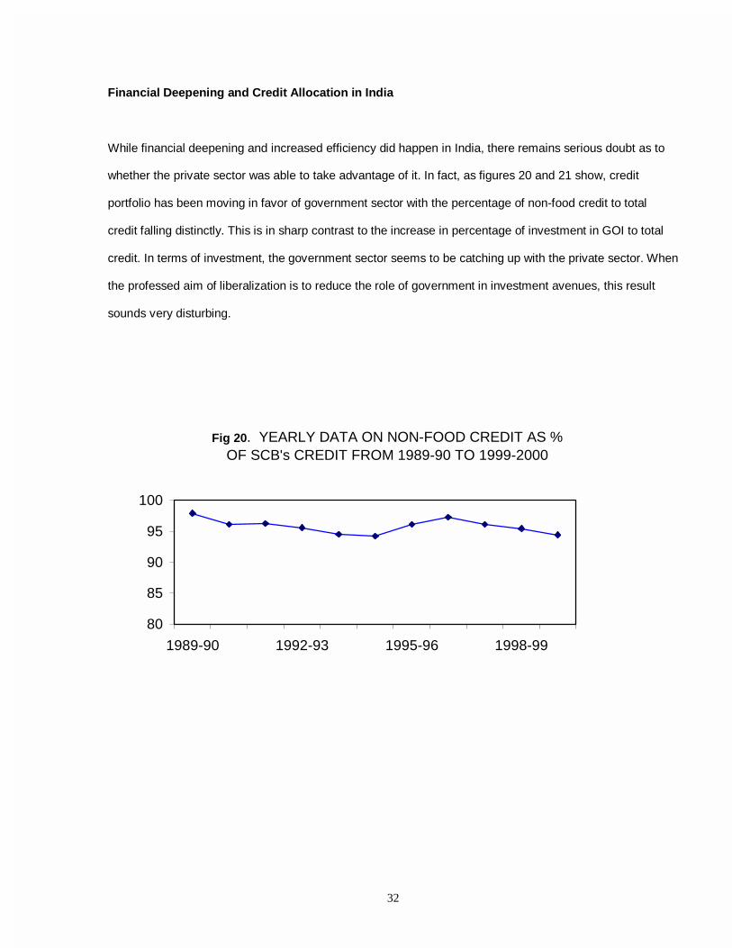
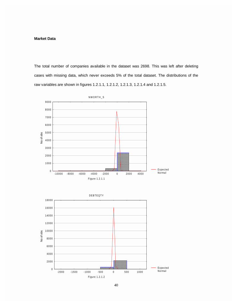
Market Data

The total number of companies available in the dataset was 2698. This was left after deleting

cases with missing data, which never exceeds 5% of the total dataset. The distributions of the

raw variables are shown in figures 1.2.1.1, 1.2.1.2, 1.2.1.3, 1.2.1.4 and 1.2.1.5.

ExpectedNorma l

N W O R T H _ S

Figure 1.2.1.1

No

of o

bs

0

1 0 0 0

2 0 0 0

3 0 0 0

4 0 0 0

5 0 0 0

6 0 0 0

7 0 0 0

8 0 0 0

9 0 0 0

- 1 0 0 0 0 - 8 0 0 0 - 6 0 0 0 - 4 0 0 0 - 2 0 0 0 0 2 0 0 0 4 0 0 0

ExpectedNorma l

D E B T E Q T Y

Figure 1.2.1.2

No

of o

bs

0

2 0 0 0

4 0 0 0

6 0 0 0

8 0 0 0

1 0 0 0 0

1 2 0 0 0

1 4 0 0 0

1 6 0 0 0

1 8 0 0 0

-2000 -1500 -1000 -500 0 5 0 0 1 0 0 0

41

ExpectedNorma l

P A T _ S

Figure 1.2.1.3

No

of o

bs

0

2 0 0 0

4 0 0 0

6 0 0 0

8 0 0 0

1 0 0 0 0

1 2 0 0 0

1 4 0 0 0

1 6 0 0 0

1 8 0 0 0

-2000 -1500 -1000 -500 0 5 0 0

ExpectedNorma l

DIV_S

Figure 1.2.1.4

No

of o

bs

0

5 0 0

1 0 0 0

1 5 0 0

2 0 0 0

2 5 0 0

3 0 0 0

3 5 0 0

4 0 0 0

4 5 0 0

5 0 0 0

5 5 0 0

6 0 0 0

-20 0 2 0 4 0 6 0 8 0 1 0 0

42

Control Market Data

The total market dataset was partitioned into two datasets by the adj. closing price / face value

ratio.

This divides up the companies into two subsets on the basis of adj. closing price >= 10

face value

Thus, those companies whose shares were trading at over 10 times their face value are

considered to be the blue chip companies while the others are the medium and poorly performing

companies, especially so far as the stock market is concerned. The first subset consisted of 251

companies after correcting for missing data and the medium to poorly performing companies

ended up with 2447 companies after deleting the missing data. The data fields were as in

previous cases. The distributions of the variables in the datasets are plotted in figures 1.2.2.1,

1.2.2.2, 1.2.2.3, 1.2.2.4, 1.2.2.5, and 1.2.2.1.1, 1.2.2.2.2, 1.2.2.3.3., 1.2.2.4.4 and 1.2.2.5.5.

ExpectedNorma l

A D J P R I C E

Figure 1.2.1.5

No

of o

bs

0

5 0 0

1 0 0 0

1 5 0 0

2 0 0 0

2 5 0 0

3 0 0 0

3 5 0 0

4 0 0 0

4 5 0 0

5 0 0 0

-1000 0 1 0 0 0 2 0 0 0 3 0 0 0 4 0 0 0 5 0 0 0 6 0 0 0 7 0 0 0 8 0 0 0

43

ExpectedNorma l

N W _ S H

Figure 1.2.2.1

No

of o

bs

0

2 0

4 0

6 0

8 0

1 0 0

1 2 0

1 4 0

1 6 0

1 8 0

2 0 0

2 2 0

2 4 0

2 6 0

2 8 0

-1000 -500 0 5 0 0 1 0 0 0 1 5 0 0 2 0 0 0 2 5 0 0 3 0 0 0 3 5 0 0

ExpectedNorma l

D E B T E Q T Y

Figure 1.2.2.2

No

of o

bs

0

2 0

4 0

6 0

8 0

1 0 0

1 2 0

1 4 0

1 6 0

1 8 0

2 0 0

2 2 0

2 4 0

-2 0 2 4 6 8 1 0 1 2

44

ExpectedNorma l

P A T _ S H

Figure 1.2.2.3

No

of o

bs

0

2 0

4 0

6 0

8 0

1 0 0

1 2 0

1 4 0

1 6 0

1 8 0

2 0 0

2 2 0

2 4 0

2 6 0

2 8 0

-200 -100 0 1 0 0 2 0 0 3 0 0 4 0 0 5 0 0

ExpectedNorma l

D IV_SH

Figure 1.2.2.4

No

of o

bs

0

2 0

4 0

6 0

8 0

1 0 0

1 2 0

1 4 0

1 6 0

1 8 0

2 0 0

2 2 0

-10 0 1 0 2 0 3 0 4 0 5 0 6 0 7 0

45

ExpectedNorma l

A D J P R I C E

Figure 1.2.2.5

No

of o

bs

0

2 0

4 0

6 0

8 0

1 0 0

1 2 0

1 4 0

1 6 0

1 8 0

2 0 0

2 2 0

2 4 0

2 6 0

2 8 0

-1000 0 1 0 0 0 2 0 0 0 3 0 0 0 4 0 0 0 5 0 0 0 6 0 0 0

ExpectedNorma l

N W O R T H _ S

Figure 1.2.2.1.1

No

of o

bs

0

1 0 0 0

2 0 0 0

3 0 0 0

4 0 0 0

5 0 0 0

6 0 0 0

7 0 0 0

8 0 0 0

- 1 0 0 0 0 - 8 0 0 0 - 6 0 0 0 - 4 0 0 0 - 2 0 0 0 0 2 0 0 0 4 0 0 0

46

ExpectedNorma l

D E B T E Q T Y

Figure 1.2.2.2.2

No

of o

bs

0

2 0 0 0

4 0 0 0

6 0 0 0

8 0 0 0

1 0 0 0 0

1 2 0 0 0

1 4 0 0 0

1 6 0 0 0

1 8 0 0 0

-2000 -1500 -1000 -500 0 5 0 0 1 0 0 0

ExpectedNorma l

P A T _ S H

Figure 1.2.2.3.3

No

of o

bs

0

2 0 0 0

4 0 0 0

6 0 0 0

8 0 0 0

1 0 0 0 0

1 2 0 0 0

1 4 0 0 0

1 6 0 0 0

-2000 -1500 -1000 -500 0 5 0 0

47

ExpectedNorma l

D IV_SH

Figure 1.2.2.4.4

No

of o

bs

0

5 0 0

1 0 0 0

1 5 0 0

2 0 0 0

2 5 0 0

3 0 0 0

3 5 0 0

4 0 0 0

4 5 0 0

5 0 0 0

5 5 0 0

-20 0 2 0 4 0 6 0 8 0 1 0 0

ExpectedNorma l

A D J P R I C E

Figure 1.2.2.5.5

No

of o

bs

0

5 0 0

1 0 0 0

1 5 0 0

2 0 0 0

2 5 0 0

3 0 0 0

3 5 0 0

4 0 0 0

-1000 0 1 0 0 0 2 0 0 0 3 0 0 0 4 0 0 0 5 0 0 0 6 0 0 0 7 0 0 0 8 0 0 0

48

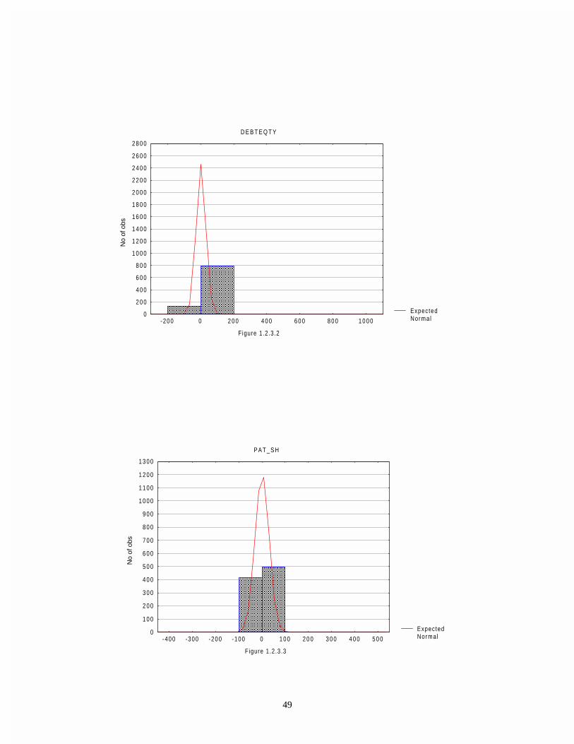
Manufacturing Sector Data

The manufacturing sector dataset consists of a set of 923 companies. In selecting this datasets

we have applied the "survival" assumption; that is, only those manufacturing companies, which

have survived the ten years 1990-2000 have been considered within the dataset. Regression run

on this dataset will thus not only be a test on the fit of the model, but also on the conditional

properties of the model subject to the ten year survival assumption. The distribution of the raw

data are plotted in figures 1.2.3.1., 1.2.3.2., 1.2.3.3., 1.2.3.4 and 1.2.3.5.

ExpectedNorma l

N W O R T H _ S

Figure 1.2.3.1

No

of o

bs

0

1 0 0

2 0 0

3 0 0

4 0 0

5 0 0

6 0 0

7 0 0

8 0 0

9 0 0

1 0 0 0

1 1 0 0

-1000 -500 0 5 0 0 1 0 0 0 1 5 0 0 2 0 0 0 2 5 0 0 3 0 0 0 3 5 0 0

49

ExpectedNorma l

D E B T E Q T Y

Figure 1.2.3.2

No

of o

bs

0

2 0 0

4 0 0

6 0 0

8 0 0

1 0 0 0

1 2 0 0

1 4 0 0

1 6 0 0

1 8 0 0

2 0 0 0

2 2 0 0

2 4 0 0

2 6 0 0

2 8 0 0

-200 0 2 0 0 4 0 0 6 0 0 8 0 0 1 0 0 0

ExpectedNorma l

P A T _ S H

Figure 1.2.3.3

No

of o

bs

0

1 0 0

2 0 0

3 0 0

4 0 0

5 0 0

6 0 0

7 0 0

8 0 0

9 0 0

1 0 0 0

1 1 0 0

1 2 0 0

1 3 0 0

-400 -300 -200 -100 0 1 0 0 2 0 0 3 0 0 4 0 0 5 0 0

50

ExpectedNorma l

D IV_SH

Figure 1.2.3.4

No

of o

bs

0

1 0 0

2 0 0

3 0 0

4 0 0

5 0 0

6 0 0

7 0 0

8 0 0

9 0 0

-10 0 1 0 2 0 3 0 4 0 5 0 6 0 7 0

ExpectedNorma l

A D J P R I C E

Figure 1.2.3.5

No

of o

bs

0

1 0 0

2 0 0

3 0 0

4 0 0

5 0 0

6 0 0

7 0 0

8 0 0

9 0 0

1 0 0 0

1 1 0 0

1 2 0 0

1 3 0 0

-1000 0 1 0 0 0 2 0 0 0 3 0 0 0 4 0 0 0 5 0 0 0 6 0 0 0

51

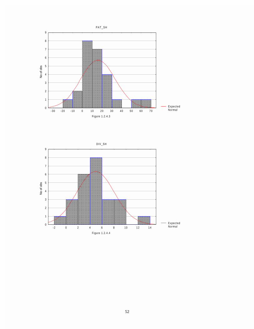
BSE 30 set of Companies

The BSE 30 set of companies at 31.12.2000 was chosen and the data for the model was set

aside for this set. Out of the 30 companies, full data were available for only 22 companies. The

distributions of the raw data are shown in figures 1.2.4.1, 1.2.4.2, 1.2.4.3, 1.2.4.4 and 1.2.4.5.

ExpectedNorma l

N W O R T H _ S

Figure 1.2.4.1

No

of o

bs

0

2

4

6

8

1 0

1 2

1 4

1 6

-100 0 1 0 0 2 0 0 3 0 0 4 0 0 5 0 0 6 0 0

ExpectedNorma l

D E B T E Q T Y

Figure 1.2.4.2

No

of o

bs

0

2

4

6

8

1 0

1 2

1 4

1 6

1 8

-1 0 1 2 3 4 5 6

52

ExpectedNorma l

P A T _ S H

Figure 1.2.4.3

No

of o

bs

0

1

2

3

4

5

6

7

8

9

-30 -20 -10 0 1 0 2 0 3 0 4 0 5 0 6 0 7 0

ExpectedNorma l

D IV_SH

Figure 1.2.4.4

No

of o

bs

0

1

2

3

4

5

6

7

8

9

-2 0 2 4 6 8 1 0 1 2 1 4

53

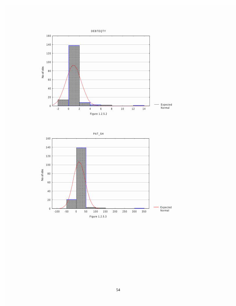
BSE 200 set of Companies

The BSE 200 set of companies at 31.12.2000 was chosen and the data for the model set aside

for this set. Out of the 200 companies in the set all data were available for 166 companies. The

distributions of the raw data are shown in the figures 1.2.5.1., 1.2.5.2., 1.2.5.3., 1.2.5.4 and

1.2.5.5.

ExpectedNorma l

A D J P R I C E

Figure 1.2.4.5

No

of o

bs

0

2

4

6

8

1 0

1 2

1 4

1 6

1 8

2 0

-1000 0 1 0 0 0 2 0 0 0 3 0 0 0 4 0 0 0 5 0 0 0 6 0 0 0 7 0 0 0 8 0 0 0

ExpectedNorma l

N W O R T H _ S

Figure 1.2.5.1

No

of o

bs

0

2 0

4 0

6 0

8 0

1 0 0

1 2 0

1 4 0

1 6 0

1 8 0

-500 0 5 0 0 1 0 0 0 1 5 0 0 2 0 0 0 2 5 0 0 3 0 0 0 3 5 0 0

54

ExpectedNorma l

D E B T E Q T Y

Figure 1.2.5.2

No

of o

bs

0

2 0

4 0

6 0

8 0

1 0 0

1 2 0

1 4 0

1 6 0

-2 0 2 4 6 8 1 0 1 2 1 4

ExpectedNorma l

P A T _ S H

Figure 1.2.5.3

No

of o

bs

0

2 0

4 0

6 0

8 0

1 0 0

1 2 0

1 4 0

1 6 0

-100 -50 0 5 0 1 0 0 1 5 0 2 0 0 2 5 0 3 0 0 3 5 0

55

ExpectedNorma l

D IV_SH

1.2.5.4

No

of o

bs

0

2 0

4 0

6 0

8 0

1 0 0

1 2 0

1 4 0

1 6 0

-10 0 1 0 2 0 3 0 4 0 5 0 6 0 7 0

ExpectedNorma l

A D J P R I C E

Figure 1.2.5.5

No

of o

bs

0

2 0

4 0

6 0

8 0

1 0 0

1 2 0

1 4 0

1 6 0

1 8 0

-1000 0 1 0 0 0 2 0 0 0 3 0 0 0 4 0 0 0 5 0 0 0 6 0 0 0 7 0 0 0 8 0 0 0

56

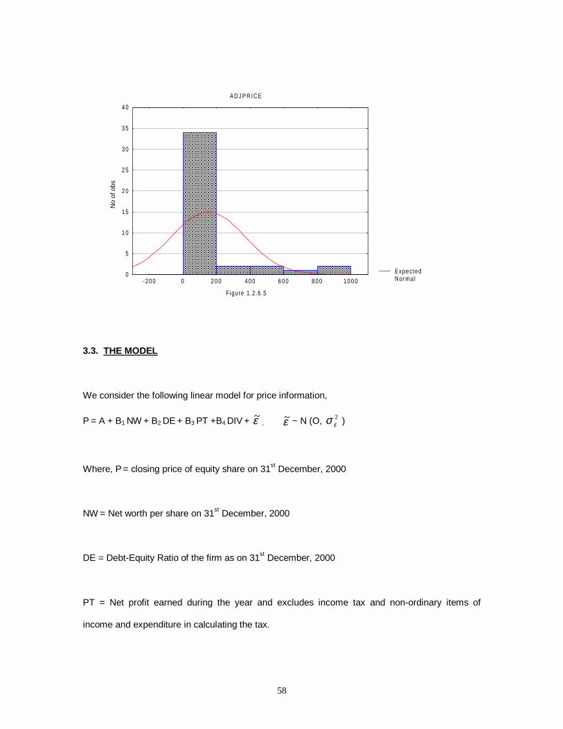
BSECG set of Companies

The BSECG set of companies (i.e., the set of companies in the BSE’s Consumer Goods Index) at

31.12.2000 was chosen and the data for the model set aside for this set. Out of the 50

companies, full dataset was available for 41 companies. The distributions of the raw variables are

provided in figures 1.2.6.1., 1.2.6.2., 1.2.6.3., 1.2.6.4 and 1.2.6.5.

ExpectedNorma l

N W O R T H _ S

Figure 1.2.6.1

No

of o

bs

0

2

4

6

8

1 0

1 2

1 4

1 6

-50 0 5 0 1 0 0 1 5 0 2 0 0 2 5 0

ExpectedNorma l

D E B T E Q T Y

Figure 1.2.6.2

No

of o

bs

0

5

1 0

1 5

2 0

2 5

3 0

3 5

-14 -12 -10 -8 -6 -4 -2 0 2 4

57

ExpectedNorma l

P A T _ S H

Figure 1.2.6.3

No

of o

bs

0

2

4

6

8

1 0

1 2

1 4

1 6

-40 -30 -20 -10 0 1 0 2 0 3 0 4 0

ExpectedNorma l

D IV_SH

Figure 1.2.6.4

No

of o

bs

0

2

4

6

8

1 0

1 2

1 4

1 6

1 8

2 0

2 2

-5 0 5 1 0 1 5 2 0

58

3.3. THE MODEL

We consider the following linear model for price information,

P = A + B1 NW + B2 DE + B3 PT +B4 DIV + ε~ , ε~ ~ N (O, 2εσ )

Where, P = closing price of equity share on 31st December, 2000

NW = Net worth per share on 31st December, 2000

DE = Debt-Equity Ratio of the firm as on 31st December, 2000

PT = Net profit earned during the year and excludes income tax and non-ordinary items of

income and expenditure in calculating the tax.

ExpectedNorma l

A D J P R I C E

Figure 1.2.6.5

No

of o

bs

0

5

1 0

1 5

2 0

2 5

3 0

3 5

4 0

-200 0 2 0 0 4 0 0 6 0 0 8 0 0 1 0 0 0

59

DIV = Dividend distributed during the year on each outstanding equity share at

31st December, 2000

ε = cross sectional error term which is a white noise and assumed to be distributed normally with

mean 0 and variance 2εσ >0.

Dividend = equity dividend distributed during year 2000 divided by the no of outstanding shares at

31.12.2000

Debt - equity =debt - equity ratio as is reflected in the Annual Returns at 31.12.2000

Profit after tax = Net profit - extraordinary income + extraordinary expenditure - other income tax.

NW describes the capital accumulated by the firm per share and is a measure of its capital stock

per share at t, which is also owner's equity per share; DE represents the debt-equity ratio and is

a measure of the financial risk associated with its capital structure; DIV represents the dividend

payments made by the firm during the year and is usually a reflection of both the profit distribution

policy of the firm as well as its liquidity situation. Although according to the Modigliani-Miller

theorem neither debt-equity ratio nor dividend distributions should affect the valuation of shares of

a firm, yet as has been argued in the literature, the ideal conditions required for Modigliani-Miller

theorem to hold do not realize in practice. For example, there are differential rates of taxes on

dividend income obtained from holding equity shares as opposed to interest income holding debt

instruments. Besides, as has been shown by Polemarchakis (1990) degree of risk aversion

amongst different participants in the financial markets should affect share pricing when one

integrates the financial and economic variables, at equilibrium. Besides, who owns debt and who

owns equity should also matter, hence bringing in questions of distribution of ownership of firms.

Dividends also have a number of reasons as to why they should affect equilibrium price of

shares. Firstly, in developing countries such as India financial markets are incomplete (on this

see Polemarchakis (1990). This may arise due to variety of reasons like asymmetric distribution

of wealth, costs of private technology and lack of information including technical expertise.

Hence, not all equity shares can be actively traded even amongst the participants in the stock

60

market. In fact it has been observed that, on average, more than 80% of the trading in financial

markets happens with respect to a select few shares of large companies and the rest of the

market is passive, not to mention shares of newly floated firms, small firms and those who cannot

list themselves with the stock exchange. Thus there is a difference in realizability between

distribution of profit in cash and trading on shares to realize capital gains. Besides, taxes on

dividends and taxes on capital gains are different. Bhattacharya (1979) has also brought out the

importance of the signaling property of dividends, i.e., medium and small companies want to

signal liquidity to go in for a history of dividend payouts. Thus inherent in dividends is the rationale

for signaling of profit, liquidity for investment and signaling of historically sound performance. In

fact, some old partial equilibrium finance models in the U.S., like the Gordon model (Gordon

(1959)), had provided justification for valuing the equity shares of a company on its dividend

payments history alone.

The importance of profit per share on the price per share does not require much argument.

Investment in shares by shareholder is done because the firm will produce profit on the

investment, which will increase the value of wealth in the form of shares, and which will be

distributed in accordance with the future contingent consumption plan of the equity holders.

Thus, the price of equity shares at equilibrium is derived from its equilibration between the

demand and supply of shares, demand being derived from NW, PT, DIV in its historical context

and supply being derived from NW, DE. The dual importance of NW is derived from the fact that

NW is both shareholders’ wealth as well as firm’s capital base. Since demand for shares (future

contingent consumption) is derived from the wealth per share owned by an equity holder, it drives

the demand for shares. At the same time, the NW is the capital base of the company, hence its

ability and necessity to attract financial capital depends on the capital it already has accumulated

in the form the net worth. Thus, the supply side of the share market is also made dependent on

NW. The capital structure composition also determines the value of shares, which a company

61

decides to issue or call back or split or offers as options. Of course, the supply side of the share

market is not only composed of new shares, but also from negative demand by existing

shareholders.

3.4. RESULTS OF GOODNESS-OF-FIT

The result of GLS regressions on the various datasets are as follows :

The Market Model

The regression results for the market model is summarised in the following table 1.4.1.1.

Table 1.4.1.1

Variable B t (2689) Level of significance

Intercept 14.845 3.606 0%

NW 0.124 2.840 0%

DE -0.007 -0.062 INSIGNIFICANT

PT 0.466 2.022 4%

DV 23.714 20.001 0%

62

The fitted line for price is presented in diagram 1.4.1.1., adjusted R2 = 0.253. The F-statistic of

229.09 with 4 d.o.f. is significant at the 1% level, therefore rejecting non-zero error. The DW-

statistic is small implying serial correlation of the residuals to be 0.026. Hence, the equilibrium

pricing equation is obtained from the fixed-point equation.

Regress ion95% conf id .

Predic ted vs. Observed Values

Dependent var iab le : ADJPRICE

Figure 1.4.1.1

Predic ted Values

Obs

erve

d V

alue

s

- 500

5 0 0

1 5 0 0

2 5 0 0

3 5 0 0

4 5 0 0

5 5 0 0

6 5 0 0

-2000 -1000 0 1 0 0 0 2 0 0 0 3 0 0 0

Regress ion95% conf id .

Predic ted vs. Observed Values

Dependent var iab le : ADJPRICE

Figure 1.4.1.2

Predic ted Values

Obs

erve

d V

alue

s

- 500

5 0 0

1 5 0 0

2 5 0 0

3 5 0 0

4 5 0 0

5 5 0 0

6 5 0 0

-1000 0 1 0 0 0 2 0 0 0 3 0 0 0 4 0 0 0 5 0 0 0 6 0 0 0

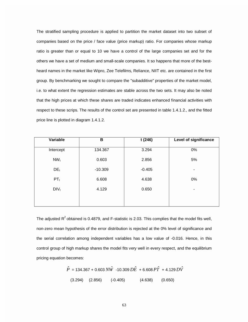
63

The stratified sampling procedure is applied to partition the market dataset into two subset of

companies based on the price / face value (price markup) ratio. For companies whose markup

ratio is greater than or equal to 10 we have a control of the large companies set and for the

others we have a set of medium and small-scale companies. It so happens that more of the best-

heard names in the market like Wipro, Zee Telefilms, Reliance, NIIT etc. are contained in the first

group. By benchmarking we sought to compare the "subadditive" properties of the market model,

i.e. to what extent the regression estimates are stable across the two sets. It may also be noted

that the high prices at which these shares are traded indicates enhanced financial activities with

respect to these scrips. The results of the control set are presented in table 1.4.1.2., and the fitted

price line is plotted in diagram 1.4.1.2.

Variable B t (246) Level of significance

Intercept

NWt

DEt

PTt

DIVt

134.367

0.603

-10.309

6.608

4.129

3.294

2.856

-0.405

4.638

0.650

0%

5%

-

0%

-

The adjusted R2 obtained is 0.4879, and F-statistic is 2.03. This complies that the model fits well,

non-zero mean hypothesis of the error distribution is rejected at the 0% level of significance and

the serial correlation among independent variables has a low value of -0.016. Hence, in this

control group of high markup shares the model fits very well in every respect, and the equilibrium

pricing equation becomes:

P̂ = 134.367 + 0.603 WN ˆ -10.309 ED ˆ + 6.608 TP ˆ + 4.129 VD ˆ

(3.294) (2.856) (-0.405) (4.638) (0.650)

64

The t-statistic is given in brackets. The insignificance of the DE coefficient suggests that the

capital structure plays an insignificant role although the sign is negative, while the DIV

coefficients have insignificant t-statistic. The other weights are significant and positive suggesting

that the contribution of NW to demand dominate its influence on supply according to the model.

The results of the general subset are summarized in table 1.4.1.3 and are as follows:

Table 1.4.1.3

Variable B t (2442) Level of significance

Intercept 15.355 3.394 0%

NW 0.115 2.371 2%

DE -0.007 -0.055 -

PT 0.519 2.015 5%

DIV 23.632 18.85 0%

The adjusted R2 =0.247, F-statistic is 201.268 and Durbin-Watson statistic is 1.948. This implies

that the model fits well with these companies too, although the R2 diminishes, while the non-zero

mean of error is rejected at 0% level and the serial correlation is low at 0.026. Hence, the

equilibrium pricing equation becomes:

P̂ = 15.355 +0.1151 WN ˆ -0.007 ED ˆ + 0.519 TP ˆ + 23.632 VD ˆ

(3.394) (2.371) (-0.055) (2.015) (18.850)

The B on DE remains insignificant and so does the negative sign. Apart from the intercept, three

other Bs become significant, including that on dividend. The scales of the Bs are lowered as the

Ps in this case are of a lower scale.

65

The fits of the predicted and actual values of P� are given in diagram 1.4.1.3.

The "subadditivity" of stock price work in this case with respect to sign except so far as dividend

is concerned.

3.5. RESULTS OF VOLATILITY

The Market Model

The residual of the cross-sectional regression model for the market database is analysed. The

R2 of 0.25 suggests that the percentage of the total variability explained by the error variability is

above 75%. The null hypothesis that the mean of the error is not 0 is rejected by the F-statistic of

201.27 which is significant at the 1% level. Therefore residual term is a white noise. Beside, the

Regress ion95% conf id .

Predic ted vs. Observed Values

Dependent var iab le : ADJPRICE

Figure 1.4.1.3

Predic ted Values

Obs

erve

d V

alue

s

- 500

5 0 0

1 5 0 0

2 5 0 0

3 5 0 0

4 5 0 0

5 5 0 0

6 5 0 0

-2000 -1000 0 1 0 0 0 2 0 0 0 3 0 0 0

66

serial correlation of errors is low at 2.6%, suggesting that the price variable is fairly uncorrelated

with the errors. The speculative component contained in the error is volatile but has mean 0,

which suggests a white noise structure. Distribution of error is plotted in diagram 1.5.1.

Control Market Data

The blue chip companies dataset gives an adjusted R2 statistic of 0.49 suggested that the

percentage of the total variability explained by the error variability is about 51%. The null

hypothesis of non-zero error is explained by the F-statistic of 60.556 at the 1% level. Therefore,

the residual term is a white noise, besides, the serial correlation is -1.5%, qualitatively replicating

the properties of the market dataset. The variance of the error term is high at 533834x102

ExpectedNorma l

Dist r ibut ion of Raw residuals

Figure 1.5.1

No

of o

bs

0

5 0 0

1 0 0 0

1 5 0 0

2 0 0 0

2 5 0 0

3 0 0 0

3 5 0 0

-3500-3000

-2500-2000

-1500-1000

-5000

5 0 01 0 0 0

1 5 0 02 0 0 0

2 5 0 03 0 0 0

3 5 0 04 0 0 0

4 5 0 05 0 0 0

5 5 0 06 0 0 0

6 5 0 0

67

suggesting that there is significant scope for analysing and reducing risk. The distribution of the

errors is plotted in diagram 1.5.2.

Manufacturing Sector Data

The manufacturing sector dataset, which has been obtained by historically conditioning on the

survival path, consists of 920 companies. The high R2 of 0.564 suggested that a significant part of

the risk in prices is explained by the variables of the model so that the residual is only about 43%.

The high F-statistic at 301.147 convincingly rejects the non-zero mean of error. Therefore the

residual term is a white noise, given the model. However, the residual sum of squares is

375290x102 which suggests significant risk residual. The serial correlation of variables is 1.5%

suggesting that the errors are white noise and therefore arises due to speculation or unfounded

variables called "sunspots". The residuals are plotted in diagram 1.5.3.

ExpectedNorma l

Dist r ibut ion of Raw residuals

Figure 1.5.2

No

of o

bs

0

2 0

4 0

6 0

8 0

1 0 0

1 2 0

1 4 0

1 6 0

1 8 0

2 0 0

-2500-2000

-1500-1000

-5000

5 0 01 0 0 0

1 5 0 02 0 0 0

2 5 0 03 0 0 0

3 5 0 04 0 0 0

4 5 0 05 0 0 0

5 5 0 06 0 0 0

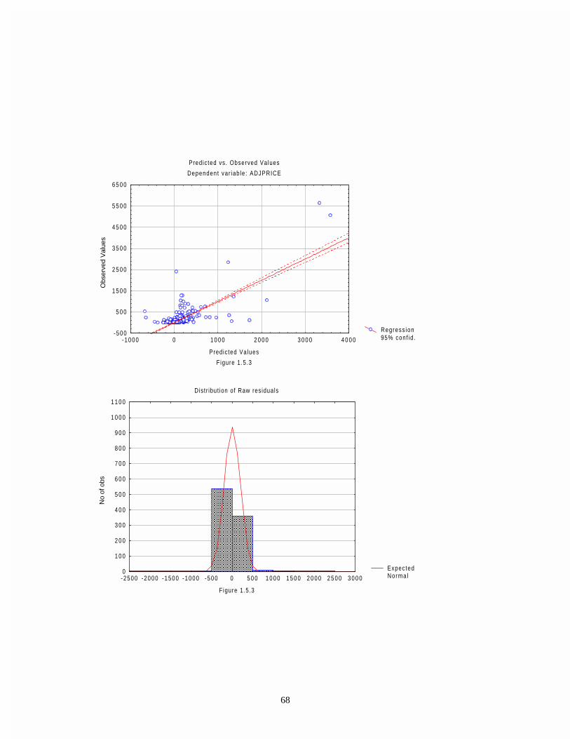
68

Regress ion95% conf id .

Predic ted vs. Observed Values

Dependent var iab le : ADJPRICE

Figure 1.5.3

Predic ted Values

Obs

erve

d V

alue

s

- 500

5 0 0

1 5 0 0

2 5 0 0

3 5 0 0

4 5 0 0

5 5 0 0

6 5 0 0

-1000 0 1 0 0 0 2 0 0 0 3 0 0 0 4 0 0 0

ExpectedNorma l

Dist r ibut ion of Raw residuals

Figure 1.5.3

No

of o

bs

0

1 0 0

2 0 0

3 0 0

4 0 0

5 0 0

6 0 0

7 0 0

8 0 0

9 0 0

1 0 0 0

1 1 0 0

-2500 -2000 -1500 -1000 -500 0 5 0 0 1 0 0 0 1 5 0 0 2 0 0 0 2 5 0 0 3 0 0 0

69

BSE 30 set of Companies

Out of the 30 companies in the dataset, full data is available on 31.12.2000 for 22 companies.

The R2 is 0.15. This means that about 85% of the total sum of squares and hence the risk in the

price variability are to be explained and controlled. The magnitude of the residual sum of squares

is 416845x102. The F-statistic is also low at 0.77, therefore the mean different from zero

hypothesis cannot be rejected. The serial correlation is -3%. However, this dataset requires a lot

to be explained. It is possible that the small size of the sample is causing the misfit. The

distribution of residuals is plotted in diagram 1.5.4.

Regress ion95% conf id .

Predic ted vs. Observed Values

Dependent var iab le : ADJPRICE

Figure 1.5.4

Predic ted Values

Obs

erve

d V

alue

s

- 1 000

0

1 0 0 0

2 0 0 0

3 0 0 0

4 0 0 0

5 0 0 0

6 0 0 0

7 0 0 0

8 0 0 0

-400 0 4 0 0 8 0 0 1 2 0 0 1 6 0 0 2 0 0 0 2 4 0 0

70

BSE 200 set of Companies

The BSE 200 set of companies contained 166 companies after deleting missing entries. The

adjusted R2 stands at 0.324 leaving about 67% of the volatility in prices in the errors. The

magnitude of the residual sum of squares is 612932x102 which means a lot of the variability

remains to explained and controlled. The F-statistic is high at 20.747 therefore the error

distribution has mean 0 at 99% level of significance. The serial correlation is low at 1%. These

suggest a white noise error whose volatility could be speculative or at best unscientific. The

distribution of residuals is shown in diagram 1.5.5.

ExpectedNorma l

Dist r ibut ion of Raw residuals

Figure 1.5.4

No

of o

bs

0

1

2

3

4

5

6

7

8

9

1 0

1 1

1 2

1 3

-3000 -2000 -1000 0 1 0 0 0 2 0 0 0 3 0 0 0 4 0 0 0 5 0 0 0 6 0 0 0 7 0 0 0

71

BSECG Set Of Companies

The third portfolio considered as the dataset is the set of companies in the BSE's Consumer

Goods Index. The model fits the dataset that consists of 41 companies with an adjusted R2 of

Regress ion95% conf id .

Predic ted vs. Observed Values

Dependent var iab le : ADJPRICE

Figure 1.5.5

Predic ted Values

Obs

erve

d V

alue

s

- 1 000

0

1 0 0 0

2 0 0 0

3 0 0 0

4 0 0 0

5 0 0 0

6 0 0 0

7 0 0 0

8 0 0 0

-1000 0 1 0 0 0 2 0 0 0 3 0 0 0 4 0 0 0 5 0 0 0

ExpectedNorma l

Dist r ibut ion of Raw residuals

Figure 1.5.5

No

of o

bs

0

1 0

2 0

3 0

4 0

5 0

6 0

7 0

8 0

9 0

1 0 0

1 1 0

1 2 0

-2000-1500

-1000-500

05 0 0

1 0 0 01 5 0 0

2 0 0 02 5 0 0

3 0 0 03 5 0 0

4 0 0 04 5 0 0

5 0 0 05 5 0 0

6 0 0 06 5 0 0

7 0 0 07 5 0 0

72

0.194, which leaves about 80% of the volatility in prices to be explained and controlled.

Considering that the entire market’s R2 is 0.25 and that of the blue chip companies controlled for

size is 0.566, there seems to be significant speculative and/or unsystematic component in this

portfolio. This could also be said of the BSE 30 portfolio although that portfolio has small size.

The F-statistic is low at the 1% level but significant for the 2% level. Besides, the serial correlation

is about 20%, which is reasonable high. The predicted and actual residuals are plotted in diagram

1.5.6.

Regress ion95% conf id .

Predic ted vs. Observed Values

Dependent var iab le : ADJPRICE

Figure 1.5.6

Predic ted Values

Obs

erve

d V

alue

s

- 100

1 0 0

3 0 0

5 0 0

7 0 0

9 0 0

-200 -100 0 1 0 0 2 0 0 3 0 0 4 0 0

ExpectedNorma l

Dist r ibut ion of Raw residuals

Figure 1.5.6

No

of o

bs

0

2

4

6

8

1 0

1 2

1 4

1 6

1 8

2 0

-400 -300 -200 -100 0 1 0 0 2 0 0 3 0 0 4 0 0 5 0 0 6 0 0 7 0 0

73

3.6. CONCLUSION

The cross-sectional model of price formation in Indian stock market at the present time is

significantly corroborated over all the datasets of companies studied. The market dataset, the

historically conditioned manufacturing sector dataset as well as the BSE 200 and BSECG

portfolios perform fairly well with respect to the model. This shows conclusively that price

formation in Indian stock markets is significantly dependent on net worth of companies as well as

their profitability and dividend payouts. However, capital structure in the form of debt/equity ratio

never gets significant weightage although the weightage is negative. It is also observed that the

B's on Net worth per share is negative. This can be explained by the decomposition of excess

demand in that the supply of share capital as well as demand depends on this variable in

opposite ways. Dividend is found to have significant weightage through demand for share capital.

It corroborates both liquidity preference and “short-sightedness" (myopia) amongst the

participants of the Indian stock market. The signaling rationale for dividends is probably rejected

due to the insignificance of Dividends in the case of "blue chip" companies where Net worth and

Profit get significant weightage. There seems to be an anomaly with respect to risk perception of

participants if debt-equity ratio and dividend payments are considered side by side for the rest of

the data sets.

The Indian stock market is however significantly described by "bounded rationality", as has been

discussed in the model section, through myopia, liquidity preference and significant volatility of

the error terms when compared within the ratio of unexplained to total sum of squares. The ratio

is reasonably high in all cases, and is significantly high in some cases, although the power of the

model and of the tests is demonstrably high. This leaves a lot of controls and long run policies

with respect to the stock market to be desired.

74

Side by side with a good explanation of the mean of share prices, is found excess volatility which

in most cases is significant suggesting presence of speculation and non-fundamental driven

activities as are referred to as "sunspot" in the Rational Expectations literature. This opens the

way for time series analysis of historical stock prices incorporating expectations into the model.

75

CHAPTER IV

FINANCIAL FRAGILITY IN STOCK MARKETS : TIME SERIES STUDY

4.1 INTRODUCTION

In estimating the Time Series properties of Price formation in stock markets, the historical data

can be divided into instantaneous, short-run, medium-run and long–run. Instantaneous analysis

requires data generated in continuous time for all variables whether relating to price formation or

fundamentals. This study however, uses discrete time data organised annually into a decade.

Hence, this study is both a short-run, as well as, a medium-run study of the stock market system.

Long-run analysis of stock market data however, requires analysis of historical epochs, which in a

semi-planned economy such as India ought to cover more than two consecutive plan periods.

This study covers a segment of the 7th Five Year Plan Period, the 8th Five Year Plan Period in full

and the first portion of the 9th Five Year Plan Period. This period also witnessed two significant

stock market crashes in the years 1993 and 1997 and the “Harshad Mehta scam” in 1992. The

time series results have to be analysed against these sets of contemporary history along with the

economic causalities outlined in the model (Bagchi(1998)).

4.2 TIME SERIES DATASET

Data for the time series regression are obtained from the Prowess database of the centre for

Monitoring Indian Economy. The database contains data for the years 1988-2000. The data have

been compiled from the audited annual accounts of public limited companies in India which

furnish Annual Returns with the Registrar of Companies and are listed on the Bombay Stock

Exchange.

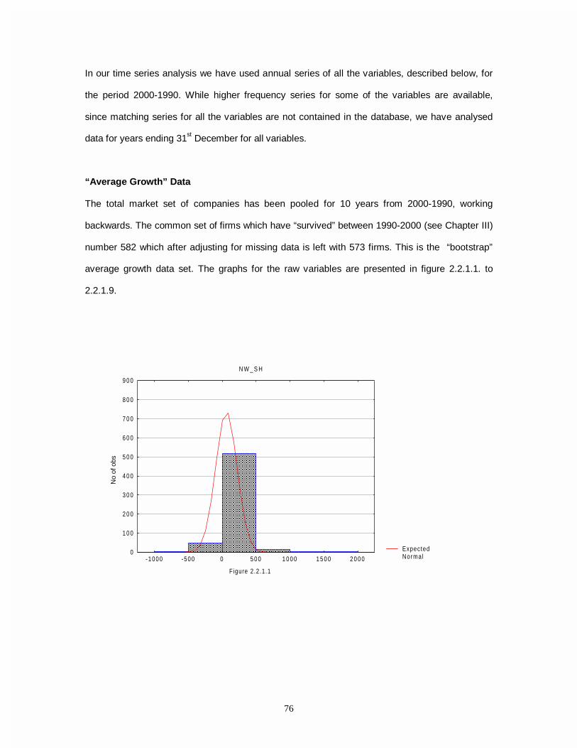
76

In our time series analysis we have used annual series of all the variables, described below, for

the period 2000-1990. While higher frequency series for some of the variables are available,

since matching series for all the variables are not contained in the database, we have analysed

data for years ending 31st December for all variables.

“Average Growth” Data

The total market set of companies has been pooled for 10 years from 2000-1990, working

backwards. The common set of firms which have “survived” between 1990-2000 (see Chapter III)

number 582 which after adjusting for missing data is left with 573 firms. This is the “bootstrap”

average growth data set. The graphs for the raw variables are presented in figure 2.2.1.1. to

2.2.1.9.

ExpectedNorma l

N W _ S H

Figure 2.2.1.1

No

of o

bs

0

1 0 0

2 0 0

3 0 0

4 0 0

5 0 0

6 0 0

7 0 0

8 0 0

9 0 0

-1000 -500 0 5 0 0 1 0 0 0 1 5 0 0 2 0 0 0

77

ExpectedNorma l

D E _ S H

Figure 2.2.1.2

No

of o

bs

0

1 0 0

2 0 0

3 0 0

4 0 0

5 0 0

6 0 0

7 0 0

8 0 0

9 0 0

-350 -300 -250 -200 -150 -100 -50 0 5 0 1 0 0

ExpectedNorma l

P T _ S H

Figure 2.2.1.3

No

of o

bs

0

1 0 0

2 0 0

3 0 0

4 0 0

5 0 0

6 0 0

7 0 0

8 0 0

-300 -200 -100 0 1 0 0 2 0 0 3 0 0 4 0 0

78

ExpectedNorma l

D I V _ S H

Figure 2.2.1.4

No

of o

bs

0

5 0

1 0 0

1 5 0

2 0 0

2 5 0

3 0 0

3 5 0

4 0 0

4 5 0

-10 0 1 0 2 0 3 0 4 0 5 0 6 0 7 0

ExpectedNorma l

G N W _ S

Figure 2.2.1.5

No

of o

bs

0

2 0 0

4 0 0

6 0 0

8 0 0

1 0 0 0

1 2 0 0

1 4 0 0

-800 -600 -400 -200 0 2 0 0 4 0 0

79

ExpectedNorma l

G D E _ S

Figure 2.2.1.6

No

of o

bs

0

5 0

1 0 0

1 5 0

2 0 0

2 5 0

3 0 0

3 5 0

4 0 0

4 5 0

5 0 0

5 5 0

6 0 0

6 5 0

-15 -10 -5 0 5 1 0 1 5 2 0 2 5 3 0

ExpectedNorma l

G P T _ S

Figure 2.2.1.7

No

of o

bs

0

1 0 0

2 0 0

3 0 0

4 0 0

5 0 0

6 0 0

7 0 0

8 0 0

-140 -120 -100 -80 -60 -40 -20 0 2 0 4 0 6 0

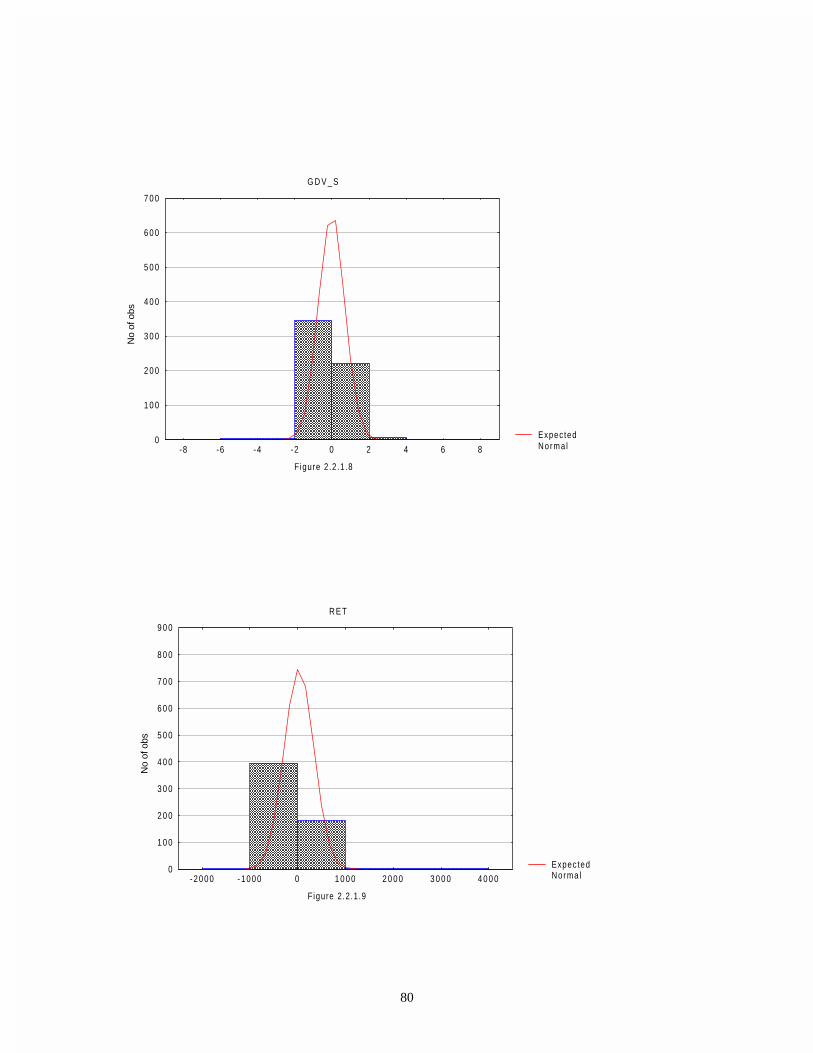
80

ExpectedNorma l

G D V _ S

Figure 2.2.1.8

No

of o

bs

0

1 0 0

2 0 0

3 0 0

4 0 0

5 0 0

6 0 0

7 0 0

-8 -6 -4 -2 0 2 4 6 8

ExpectedNorma l

R E T

Figure 2.2.1.9

No

of o

bs

0

1 0 0

2 0 0

3 0 0

4 0 0

5 0 0

6 0 0

7 0 0

8 0 0

9 0 0

-2000 -1000 0 1 0 0 0 2 0 0 0 3 0 0 0 4 0 0 0

81

Annual Price Differential Data

One period annual price differential (Return) datasets for the annual growth models 2000 –1999

to 1991-1990 are presented in the form of correlation matrix in table 2.2.2.1. A casual look at the

correlation gives an approximate idea of the nature of relationship existing between the various

variables over the annual partitions of the 10-year period.

Table 2.2.2.1

RET_1Y RET_2Y RET_3Y RET_4Y RET_5Y RET_6Y RET_7Y RET_8Y RET_9Y RET_10Y RET_1Y 1.00 -.04 .00 .02 -.01 -.01 .01 .00 .01 .00 RET_2Y -.04 1.00 -.05 .01 .01 .02 -.00 -.01 -.01 -.03 RET_3Y .00 -.05 1.00 .03 -.02 .01 .02 .05 .02 -.01 RET_4Y .02 .01 .03 1.00 .01 -.02 .01 .01 -.01 -.04 RET_5Y -.01 .01 -.02 .01 1.00 -.03 .00 -.02 .00 .05 RET_6Y -.01 .02 .01 -.02 -.03 1.00 .02 .02 .04 .01 RET_7Y .01 -.00 .02 .01 .00 .02 1.00 -.00 -.01 -.01 RET_8Y .00 -.01 .05 .01 -.02 .02 -.00 1.00 -.03 -.01 RET_9Y .01 -.01 .02 -.01 .00 .04 -.01 -.03 1.00 -.01 RET_10Y

.00 -.03 -.01 -.04 .05 .01 -.01 -.01 -.01 1.00

No correlations are significant at p < .05000

Manufacturing Sector Data

The only industry that has been considered in isolation from the market dataset is the

manufacturing sector. The reason being that the only sector that has a large number of surviving

firms between 1990 & 2000 is this sector. Three stages in the algorithm are carried out with

respect to this dataset. The 2000 – 1990 average growth model is fitted as also the 2000 –1999

annual growth model is fitted. The fits, as well as the errors, are then compared to ensure that the

errors are uncorrelated. The total number of firms in the first data set is 517 and in the other case

is 1925. The correlation matrices with respect to the two growth models are given in tables

2.2.3.1 and 2.2.3.2.

Table 2.2.3.1

NW_SH90 DE_SH90

PT_SH90

DIV_SH90 GNW_S10Y GDE_S10Y

GPT_S10Y

GDV_S10Y RET10Y

82

NW_SH90 1.000000 .025183 .740111 .851955 .114692 -.032914 -.100677 -.429485 .210495 DE_SH90 .025183 1.000000 .018750 .010412 .019033 -.777652 .012947 .008249 .014449 PT_SH90 .740111 .018750 1.000000 .706037 .139353 -.038373 -.218449 -.450747 .071874 DIV_SH90 .851955 .010412 .706037 1.000000 -.113054 -.009213 -.306639 -.658594 .062606 GNW_S10Y .114692 .019033 .139353 -.113054 1.000000 -.008633 .881516 .413916 .355693 GDE_S10Y -.032914 -.777652 -.038373 -.009213 -.008633 1.000000 .006541 -.015088 -.016135 GPT_S10Y -.100677 .012947 -.218449 -.306639 .881516 .006541 1.000000 .463758 .339531 GDV_S10Y -.429485 .008249 -.450747 -.658594 .413916 -.015088 .463758 1.000000 .439172 RET10Y .210495 .014449 .071874 .062606 .355693 -.016135 .339531 .439172 1.000000

Table 2.2.3.2

NW_SH99

DE_SH99 PT_SH99

DIV_SH99 GNW_S1Y GDE_S1Y

GPT_S1Y GDV_S1Y

RET_1Y

NW_SH99 1.000000 .006132 .732348 .440819 .618084 -.000103 .285385 -.010703 -.212520 DE_SH99 .006132 1.000000 .014161 -.001055 .012673 -.339267 .004004 .000673 .003175 PT_SH99 .732348 .014161 1.000000 .289349 .526261 -.008514 -.206490 -.017957 -.157580 DIV_SH99 .440819 -.001055 .289349 1.000000 .035746 -.001292 -.072465 -.565834 -.382219 GNW_S1Y .618084 .012673 .526261 .035746 1.000000 -.007056 .427272 .287532 -.107605 GDE_S1Y -.000103 -.339267 -.008514 -.001292 -.007056 1.000000 -.002271 -.000435 .001055 GPT_S1Y .285385 .004004 -.206490 -.072465 .427272 -.002271 1.000000 .163399 .063614 GDV_S1Y -.010703 .000673 -.017957 -.565834 .287532 -.000435 .163399 1.000000 -.019667 RET_1Y -.212520 .003175 -.157580 -.382219 -.107605 .001055 .063614 -.019667 1.000000

4.3 TIME SERIES MODEL

We consider the following time series model for dynamic price formation in Indian stock markets.

Pt+1 Pt = At +B1t NWt + B2t DEt + B3t PTt + B4t DIVt

B5t Et û 1:t + B6t Et û '(t + B7t Et û 37t + B8t Et û ',9t

+ η~ t , η~ t ∼ 1 ���1 �

2

t)

where, Pt = closing price of shares at 31st December of the year t,

NWt = Net worth per outstanding equity share at 31st December of the year t,

PTt = Profit for the year t per outstanding equity share at 31st December of the year t,

DEt = Debt Equity ratio at 31st December of the year t,

DIVt = Dividend declared during year t per outstanding equity share at 31st December of

the year t

83

û 1:t = NWt +1 - NWt , is the first forward difference in NW,

û 37t = PTt +1 - PTt , is the first forward difference in PT,

û '(t = DEt +1 - DEt, is the first forward difference in DE,

û ',9t = DIVt +1 - DIVt is the first forward difference in DIV

Et is the forward looking Rational Expectations operator with respect to 31st December of year t.

ηt LV D UDQGRP HUURU WHUP QRUPDOO\ GLVWULEXWHG ZLWK PHDQ � DQG YDULDQFH PDWUL[ 1 �

2

t >0

We shall jointly test for the fit of the model as well as the properties of the error terms

hypothesized, with annual data over the period 1990-2000.

The econometric testing of a time series model of this form, which consists of a large cross–

section of companies at any given t, can be carried out along two directions. The first method is

the traditional Vector Auto Regression method of the Box–Jenkins type. In such a method the

entire panel data pooled across firms and time periods has to be studied in integrated form to

give GLS estimates by the ARIMA model. This has the potential dimensionality cost of there

being around 2500 firms for each of the years 1990 –2000 with twelve variables, which could

become a 2500 X 10 X 12 matrix requiring high computing time and memory costs. Besides,

with a linear model specification such as ours the nonlinearity involved in the historical behavior

of stock prices would not be readily evident till we change our specification and fit a nonlinear

model all over again. This prompts us to carry out the Time-Series GLS regression in a “ nested”

procedure similar in many respects with that suggested by Granger & Newbold (1977) and

consists of the following algorithm. This algorithm uses the residual matrix of nested models to

set up an objective function based on correlations amongst nested residuals. While this

procedure helps in time series estimation of the parameters along the Granger et. al. approach, it

also provides a procedure for estimating TVP (Time Varying Parameter) problems as discussed

in Rao (2000), without using any exogenous cost minimisation objectives.

84

In the first step we break up the pooled time series ARIMA model into nested models, identified

by years, as follows:

[ Pt+1 - Pt ] = [ At + ∑=

4

1iitB historical variable it + ∑

=

8

5iitB expectation variable it + ηt]

C ⊗ T

where C is the no of companies in the data set, T is the time “ horizon” which in this case is

1990-2000 and Bit is the coefficient on historical variable i at time t where i is the indicator as

follows:

i=1 ⇒ NW

i=2 ⇒ DE

i=3 ⇒ PT

i=4 ⇒ DIV

The historical variables are as given above, the expectation variables follow exactly the same

identification i.e.

i=5 ⇒ Et û 1:

i=6 ⇒ Et û '(

i=7 ⇒ Et û 37

i=8 ⇒ Et û ',9

This is the basic time series model.

The next step we break up this general ARIMA (1,1,1) specification into first a “bootstrap”

average growth model as follows :

P2000 – P1990 = A + B1 NW1990 + B2 DE1990 + B3 PT1990 + B4 DIV1990 + B5 E1990 û 1:2000-1990

85

+ B6 E1990 û '( 2000-1990 + B7 E1990 ûPT 2000-1990 + B8 E1990 û',92000-1990 + η~

Where, E1990 û1:2000-1990 = NW2000 - NW1990 ,

E1990 û'(2000-1990 = DE2000 - DE1990,

E1990 û372000-1990 = PT2000 - PT1990

E1990 û',92000-1990 = DIV2000 -DIV1990

Thus, here the dependant variable is the total price differential over the decade. Any of the

coefficients B5 to B8 is the "average growth" coefficient in the sense for e.g.

B5 E1990 û 1: 2000-1990 = 10 B5 E1990 û1:2000-1990

10

This model seems as the benchmark "bootstrap" model for the decade of the 90s.

In the third step the linear growth assumption along with the 10-year horizon assumption is

relaxed to test a set of ten "nested" models, one for each year as follows :

Ret n = An + ∑=

4

1iinB historical variable i + ∑

=

8

5iinB expectation variable i

+ nε~ , nε~ ~ N(0, 1 0

2

t), n = 1999 ….. 1990.

and growth is taken over 1 year periods working back from 2000 for each n , and expectations is

forward looking over the one year.

For example,

B15 E1 û1:1 = B1999,5

(NW2000-NW1999) and so on

Retn =Pn+1 – Pn

86

Granger & Newbold (1977) argue, this is a valid procedure for obtaining the Time Series

SURSHUWLHV RI 6WRFN 3ULFH� SURYLGHG WKH UHVLGXDO PDWUL[ >/n ] does not show significant serial

correlation. Therefore the final step in this algorithm is to check for the corrHODWLRQ LQ WKH >/n ]

matrix from the ten nested models obtained in step 3. If the significance of serial correlation is low

then this is also a algorithmic procedure for cointegration of stock price variables. We test these

hypotheses in the following sections.

4.4 TIME SERIES RESULTS (GOODNESS-OF-FIT)

The "Average Growth " Model

The average growth model for the ten year period 2000 - 1990 is presented. The dataset consists

of the entire market data and the partitioned manufacturing data. Both the set of results serve as

a bootstrapping benchmark for the linear model specification in the stage 1 of the modeling

algorithm.

The Market Data

The total number of "surviving" firms between the decade 31.12.90 and 31.12.2000 is 573 in the

total market dataset. The average growth model was run on the set taking annual series as has

been discussed. The results are summarised in the following table:

87

Variable B t (573) Level of

significance

Intercept

NW1990

DE1990

PT1990

DIV1990

GNW2000-1990

GDE2000-1990

GPT2000-1990

GDV2000-1990

-16.47

- 0.165

0.085

2.819

23.30

-2.909

0.875

21.355

326.194

-1.298

-1.225

0.079

4.33

6.823

-3.227

0.106

4.415

14.356

Insignificant

Insignificant

Insignificant

1%

0%

1%

Insignificant

1%

0%

Thus, the estimated equation becomes:

P2000 - P1990 = -16.47 - 0.165NW1990 +0.085 DE1990 + 2.819 PT1990 + 23.30 DIV1990

(-1.298) (-1.225) (0.079) (4.33) (6.823)

-2.909 GNW2000-1990 + 0.875 GDE2000-1990 +21.355 GPT2000-1990 + 326.194 GDV2000-1990

(-3.227) (0.106) (4.415) (14.356)

The R2 is high at 0.36 and the F-statistic is high at 42.09366 which is significant at the 0% level

and the serial correlation of the residuals is low at 0.05 suggesting a good fit for the model.

The signs of the significant weights on the initial profit (PT1990), initial dividend (DIV1990) and in

their growth is substantiated by the model, while the negative weightage on GNW2000-1990 seems

88

to be arising due to the predominance of the supply factors over demand in the fixed point

equation of the model. The fitted "price differential" line is plotted in fig. 2.4.1.1. as RET 10Y.

Manufacturing Sector Data

The total number of "surviving " firms in the manufacturing sector dataset over the period 2000 -

1990 is 517. The average growth linear model was run on the dataset taking annual series, as

has been discussed, to obtain the GLS estimates. The results are presented in the following

table:

Regress ion95% conf id .

Predic ted vs. Observed Values

Dependent var iab le : RET10Y

Figure 2.4.1.1

Predic ted Values

Obs

erve

d V

alue

s

- 1 500

-500

5 0 0

1 5 0 0

2 5 0 0

3 5 0 0

4 5 0 0

-1400 -800 -200 4 0 0 1 0 0 0 1 6 0 0 2 2 0 0

89

Variable B t (573) Level of

significance

Intercept

NW1990

DE1990

PT1990

DIV1990

GNW2000-1990

GDE2000-1990

GPT2000-1990

GDV2000-1990

-20.47

0.215

0.069

2.967

30.885

-5.987

1.273

37.317

441.713

-1.425

1.003

0.061

4.04

6.504

-5.586

0.146

6.716

16.69

Insignificant

Insignificant

Insignificant

1%

0%

0%

Insignificant

0%

0%

The R2 is high at 0.46.

The graph of the plot of the fitted price differential is shown in figure 2.4.1.2.

Regress ion95% conf id .

Predic ted vs. Observed Values

Dependent var iab le : RET10Y

Figure 2.4.1.2

Predic ted Values

Obs

erve

d V

alue

s

- 1 000

0

1 0 0 0

2 0 0 0

3 0 0 0

4 0 0 0

5 0 0 0

6 0 0 0

-1500 -1000 -500 0 5 0 0 1 0 0 0 1 5 0 0 2 0 0 0 2 5 0 0 3 0 0 0

90

Annual Price Differential Data

In keeping with the algorithmic approach to the time series analysis of this paper we regress the

model on annual data for the periods 2000-1990. The results of the regression for the various

periods within the decade are summarized in the following table 2.4.1.3.1.

91

period Inter- cept

NW DE PT DIV GNW GDE GPT GDIV R2 F DW

00-99 -4.2 (-1.39)

-0.021 (-0.46)

0.023 (0.163)

0.419 (2.30)

-16.87 (-19.14)

-0.33 (-3.54)

0.01 (0.11)

0.977 (5.01)

-13.49 (-11.40)

0.19 73.24 1.80

99-98 22.88 (5.74)

0.098 (2.79)

-0.05 (-0.14)

1.02 (7.15)

7.54 (6.78)

0.21 (3.44)

-0.04 (-0.24)

1.15 (6.45)

6.29 (5.04)

0.08 34.38 1.76

98-97 3.38 (3.84)

0.019 (4.57)

-0.01 (-0.11)

0.18 (3.47)

-3.16 (11.86)

0.34 (-8.14)

0.00 (0.08)

0.61 (8.4)

1.28 (4.07)

0.08 39.18 1.97

97-96 7.52 (5.72)

0.04 (6.08)

-0.15 (-1.06)

-0.39 (-8.02)

-11.21 (-28.23)

-0.56 (-25.18)

0.01 (0.17)

-0.5 (-5.3)

7.02 (9.03)

0.34 226.20 1.97

96-95 3.01 (1.71)

-0.31 (-11.24)

-0.00 (-0.001)

1.13 (9.61)

-7.52 (-10.20)

-0.55 (-8.23)

-0.01 (-0.05)

-0.63 (-6.92)

4.04 (3.03)

0.27 147.86 2.02

95-94 -13.15 (-3.45)

-0.68 (-11.48)

0.01 (0.07)

1.35 (6.19)

-5.13 (-3.54)

-0.53 (-7.21)

-0.02 (-0.16)

2.14 (11.78)

-14.11 (-6.73)

0.24 89.38 1.99

94-93 37.6 (3.75)

1.19 (8.85)

-0.07 (-0.11)

-1.58 (-3.61)

-14.11 (-4.61)

0.13 (0.68)

-0.05 (0.09)

0.36 (0.85)

-11.4 (-1.99)

0.09 19.29 1.97

93-92 6.55 (2.50)

0.07 (2.44)

-0.16 (-0.44)

-0.07 (-0.66)

0.699 (1.16)

-0.06 (-1.71)

-0.005 (0.06)

0.323 (4.23)

4.962 (3.385)

0.07 11.67 2.02

92-91 0.79 (0.26)

0.058 (1.957)

-0.273 (-0.805)

0.52 (4.37)

5.82 (6.926)

0.008 (0.157)

-0.293 (-0.861)

1.251 (9.167)

8.552 (6.187)

0.26 42.55 2.12

91-90 20.12 (3.86)

0.09 (1.67)

0.04 (0.07)

-0.53 (-2.43)

8.84 (6.36)

-0.29 (-2.33)

0.034 (0.07)

0.64 (3.074)

2.883 (2.98)

0.14 17.40 2.11

Table 2.4.1.3.1

92

The fit of the ten annual models never perform better than the average growth model over the

10-year horizon in terms of R2, which has a significantly high R2 at 0.36. Besides, the F-statistic is

significant for the average growth rational expectations model over 10 years and the serial

correlation of residuals is also low, rejecting a non-linear fit to the pricing equation through annual

series in favour of a linear fit. This inference is correct based on the comparison of the two sets of

models, because as required by Granger & Newbold (1977), the error correlation matrix among

the nested residuals as given in table 2.4.1.3.2 does not show significant serial correlation.

Table 2.4.1.3.2

E1 E2

E3

E4

E5

E6

E7

E8

E9

E10

E1 1.00 -.04 -.01 .01 -.07* .01 .04 .07* -.01 -.00 E2 -.04 1.00 -.03 -.04 -.04 .01 .02 -.02 -.00 -.00 E3 -.01 -.03 1.00 -.01 -.01 -.03 -.03 -.02 -.00 .04 E4 .01 -.04 -.01 1.00 .00 .00 .01 -.02 .01 .02 E5 -.07* -.04 -.01 .00 1.00 -.03 .02 .02 -.02 .00 E6 .01 .01 -.03 .00 -.03 1.00 .02 .05 -.01 -.01 E7 .04 .02 -.03 .01 .02 .02 1.00 .03 .01 .16* E8 .07* -.02 -.02 -.02 .02 .05 .03 1.00 -.04 -.02 E9 -.01 -.00 -.00 .01 -.02 -.01 .01 -.04 1.00 .00 E10 -.00 -.00 .04 .02 .00 -.01 .16* -.02 .00 1.00 Marked correlations are significant at p < 0.05000

This rejects the hypothesis of significant correlation with only 3 out of 45 correlations being

significant and that too with a maximum magnitude of 0.16. This inference is also true when one

compares the manufacturing sector for its fit over 2000-1990 with 2000-1999 the most recent one

year. The results for the 2000 -1999 period are given in table 2.4.1.3.3.

93

Variable B t-statistic Level of significance

Intercept

NW99

DE99

PT99

DIV99

GNW

GDE

GPT

GDV

-3.91

0.007

0.02

0.327

-21.09

-0.27

0.005

0.832

-18.197

-1.057

0.183

0.129

1.564

-19.967

-2.483

0.065

3.733

-13.214

Insignificant

Insignificant

Insignificant

Insignificant

0%

2%

Insignificant

1%

0%

Adjusted R2 is 0.23.

Here also the average growth ten-year model obtains a better fit, suggesting that the longer term

linear rational expectations model performs better. In other words, the cointegrated price

variables fit better in both cases with a linear average growth trend. Both these observations are

somewhat incongruous with a high and significant weightage on historical dividends and dividend

growths, which suggest high liquidity preference and therefore "myopia".

The fitted lines for the ten year average growth model and for the 2000-1999 model for the entire

market data set are presented in figures 2.4.1.3.1 and 2.4.1.3.2.

94

4.5 TIME SERIES RESULTS (VOLATILITY)

An analysis-of-fit of the model to the time series data reveals that on average a good part of the

dynamic price differential is explained by the set of historical and rational expectations variables.

Regress ion95% conf id .

Predic ted vs. Observed Values

Dependent var iab le : RET_10Y

Figure 2.4.1.3.1

Predic ted Values

Obs

erve

d V

alue

s

- 400

2 0 0

8 0 0

1 4 0 0

2 0 0 0

2 6 0 0

3 2 0 0

-300 -200 -100 0 1 0 0 2 0 0 3 0 0 4 0 0 5 0 0 6 0 0

Regress ion95% conf id .

Predic ted vs. Observed Values

Dependent var iab le : RET_1Y

Figure 2.4.1.3.2

Predic ted Values

Obs

erve

d V

alue

s

- 3 500

-2500

-1500

-500

5 0 0

1 5 0 0

2 5 0 0

-1800 -1400 -1000 -600 -200 2 0 0 6 0 0

95

The result shows an overall R2 (adjusted for serial autocorrelation and heteroskedasticity) of 0.36

with significant t-statistic on all but the debt-equity variables. The fit of the model is more striking

in the case of the manufacturing sector. However, it still leaves a lot of volatility to be explained.

When it comes to an analysis of the volatility in the residuals it is observed that as was true in the

cross-section data the F-statistic and DW-statistic are both significantly high, leaving therefore the

variance to be analysed only. Further an analysis of the correlation matrix across the various

"nested " models of annual duration suggest that the across the period serial correlations are

insignificant. This not only points to the existence of a ten year set of data cointegrated with the

price differentials but also to the fact that residuals are "random walks" over time at least within

this ten year history. However, after the conditioning on the variables of the model the errors do

follow a "random walk" pattern. Variability reducing policies targeted at the short-term annual

performances are necessary in this respect. What type of instruments co-vary with these annual

residuals so as to reduce them is a question which requires consideration.

Behaviourally speaking "myopia" through dividend and expected dividend dependence operates

in contrast to the overriding performance of the longer term "average growth " model. This is an

anomaly like the “Hindu” rate of growth in India. However, the significant variance of the residual

sum of squares does certainly point direction to speculative "gambling" and "sunspot"

components in the stock market. The plot of the distribution of residuals in the ten year average

growth model for the total market and manufacturing sector datasets are presented in figures

2.5.1 and 2.5.2.

96

ExpectedNorma l

Dist r ibut ion of Raw residuals

Figure 2.5.1

No

of o

bs

0

5 0

1 0 0

1 5 0

2 0 0

2 5 0

3 0 0

3 5 0

4 0 0

4 5 0

5 0 0

5 5 0

6 0 0

-800-600

-400-200

02 0 0

4 0 06 0 0

8 0 01 0 0 0

1 2 0 01 4 0 0

1 6 0 01 8 0 0

2 0 0 02 2 0 0

2 4 0 02 6 0 0

2 8 0 0

ExpectedNorma l

Dist r ibut ion of Raw residuals

Figure 2.5.2

No

of o

bs

0

5 0

1 0 0

1 5 0

2 0 0

2 5 0

3 0 0

3 5 0

4 0 0

4 5 0

5 0 0

-2000 -1500 -1000 -500 0 5 0 0 1 0 0 0 1 5 0 0 2 0 0 0 2 5 0 0 3 0 0 0 3 5 0 0

97

4.6 CONCLUSION

The structure of the financial markets in India is described by the presence of historical real (net

worth per share, profitability per share ) and financial (debt-equity ratio, dividend distributed per

share ) variables as well as their rationally expected growth values over the future. This structure

is cointegrated with the stock price so that it may be said that in corporate governance, price is an

important consideration in making decisions on the above explanatory variables at the corporate

level. This is in the light of the fact that although there is a lot of residual volatility, lack of

explosive components makes cointegration possible. If one compares it with the fact that the

relationships within the model are stronger in the annual data in periods distant from 1993 and

1997, the two periods of crashes and other significant events, as discussed in the beginning

(which therefore opens up areas of further analysis of structural breaks), then the linear fit, on

average, suggests that, albeit a high degree of volatility, "planned competition" has been

responsible in preventing markets from crashing more often, and changing the overall structure of

the interplay between price formation, history and expectations along with it.

98

CHAPTER V

FINANCIAL FRAGILITY IN STOCK MARKETS: MACRO-MONETARY POLICY ANALYSIS

5.1. INTRODUCTION

The previous chapters were involved with the estimation of the extent of financial fragility in Indian

financial markets. In this chapter, the possible impact of monetary policy in controlling the fragility

through price formation is sought to be estimated. As monetary policy operates through interest

rates mainly, in so far as the stock market is concerned, this chapter estimates the impact of

monetary policy on stock prices through the estimation of interest cost sensitivity of stock prices.

Interest cost has two components, viz. interest rate and the volume of debt. In estimating

sensitivity to monetary policy changes, both the components of interest as mentioned above can

be controlled by the Reserve Bank of India through various policy tools, for example, altering the

PLR, changing the interest rate on lending by commercial banks to companies which are bank

financed. Since a change in the nature of priorities in granting loans alters the volume of term

loans available for various types of projects by such borrowing companies, it is sought justified to

consider the entire interest cost component of corporate expenditure separately as an

explanatory variable in its own right in estimating the pricing equation of the stock market over

time. While debt does not consist of borrowings from banks only, which is under the direct control

of the Reserve Bank of India, debt costs operating through competitive debt markets are indirectly

controlled by the Reserve Bank of India and the Ministry of Finance through its monetary policy

and the operation of the money multiplier.

In estimating the time series properties of price formation in stock markets with interest cost as an

explanatory variable, interest cost is differentiated from the profit term by addition and identified

separately. The historical data has been, as in the previous chapter, divided into instantaneous,

short-run, medium-run and long–run data. Instantaneous analysis requires data generated in

continuous time for all variables whether relating to price formation or fundamentals. This study,

99

however, uses discrete time data organised annually into a decade. Hence, this study is both a

short-run, as well as, a medium-run study of the stock market system, including interest cost as a

fundamental variable. Long-run analysis of stock market data however, requires analysis of

historical epochs, which in a semi-planned economy such as the Indian economy, ought to cover

more than two consecutive plan periods. This study covers a segment of the 7th Five Year Plan

Period, the 8th Five Year Plan Period in full and the first portion of the 9th Five Year Plan Period.

This period also witnessed two significant stock market crashes in the years 1993 and 1997 and

the “Harshad Mehta scam” in 1992. The time series results have to be analysed against these

sets of contemporary history along with the economic causalities outlined in the model (Tobin

(1972), Bagchi (1998)).

5.2. TIME SERIES DATA

Data for the time series regression are obtained from the Prowess database of the Centre for

Monitoring Indian Economy. The database contains data for the years 1988-2000. The data have

been compiled from the audited annual accounts of public limited companies in India, which

furnish annual returns with the Registrar of Companies and are listed on the Bombay Stock

Exchange.

In our time series analysis we have used annual series of all the variables, described below, for

the period 2000-1990. While higher frequency series for some of the variables are available,

since matching series for all the variables are not contained in the database, we have analysed

data for years ending 31st December for all variables.

“Average Growth” Data

100

The total market set of companies has been pooled for 10 years from 2000-1990, working

backwards. The common set of firms, which have “survived” between 1990-2000 (see Chapter

IV), numbers 582 which after adjusting for missing data is left with 571 firms. This is the

“bootstrap” average growth dataset. The graphs for the raw variables are presented in figure

3.2.1.1 to 3.2.1.11

ExpectedNormal

NW_SH90

Figure 3.2.1.1

No

of o

bs

0

100

200

300

400

500

600

700

800

900

-1000 -500 0 500 1000 1500 2000

ExpectedNormal

DE_SH90

Figure 3.2.1.2

No

of o

bs

0

100

200

300

400

500

600

700

800

900

-350 -300 -250 -200 -150 -100 -50 0 50 100

101

ExpectedNormal

PI_SH90

Figure 3.2.1.3

No

of o

bs

0

50

100

150

200

250

300

350

400

450

500

550

600

-300 -200 -100 0 100 200 300 400 500 600 700

ExpectedNormal

IC_SH90

Figure 3.2.1.4

No

of o

bs

0

50

100

150

200

250

300

350

400

450

500

550

600

650

-100 0 100 200 300 400 500

102

ExpectedNormal

DV_SH90

Figure 3.2.1.5

No

of o

bs

0

50

100

150

200

250

300

350

400

450

-10 0 10 20 30 40 50 60 70

ExpectedNormal

GNW_S10Y

Figure 3.2.1.6

No

of o

bs

0

200

400

600

800

1000

1200

1400

-8000 -6000 -4000 -2000 0 2000 4000

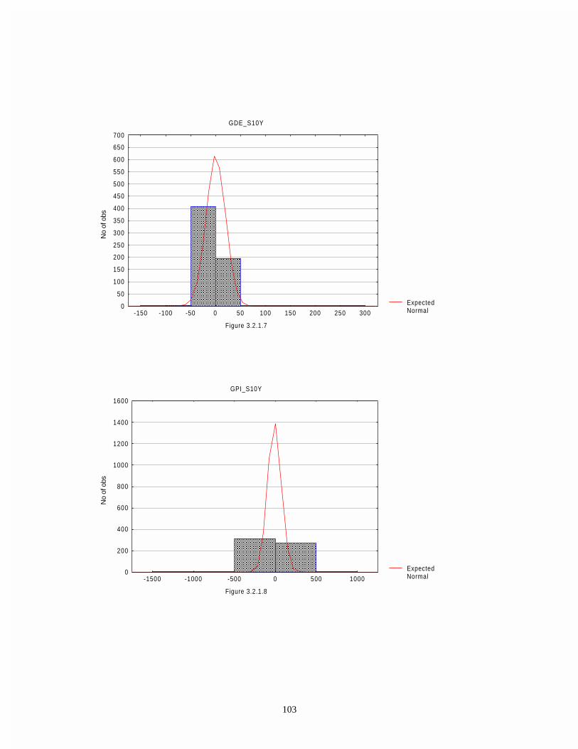
103

ExpectedNormal

GDE_S10Y

Figure 3.2.1.7

No

of o

bs

0

50

100

150

200

250

300

350

400

450

500

550

600

650

700

-150 -100 -50 0 50 100 150 200 250 300

ExpectedNormal

GPI_S10Y

Figure 3.2.1.8

No

of o

bs

0

200

400

600

800

1000

1200

1400

1600

-1500 -1000 -500 0 500 1000

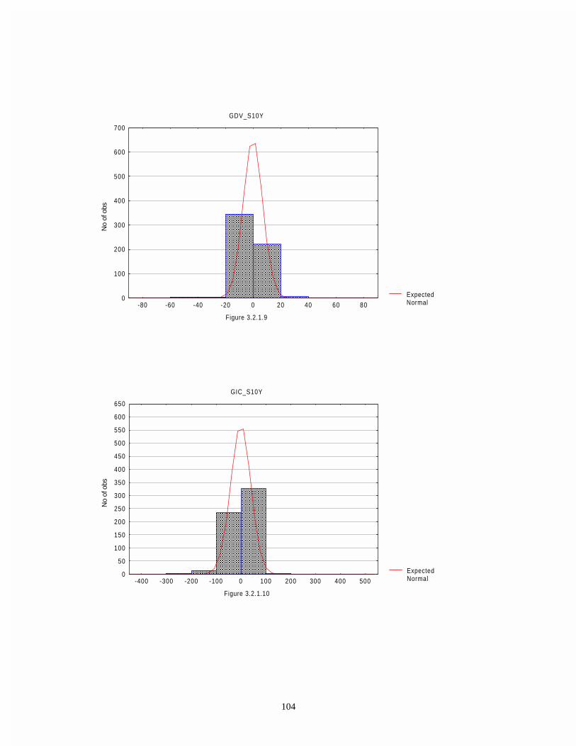
104

ExpectedNormal

GDV_S10Y

Figure 3.2.1.9

No

of o

bs

0

100

200

300

400

500

600

700

-80 -60 -40 -20 0 20 40 60 80

ExpectedNormal

GIC_S10Y

Figure 3.2.1.10

No

of o

bs

0

50

100

150

200

250

300

350

400

450

500

550

600

650

-400 -300 -200 -100 0 100 200 300 400 500

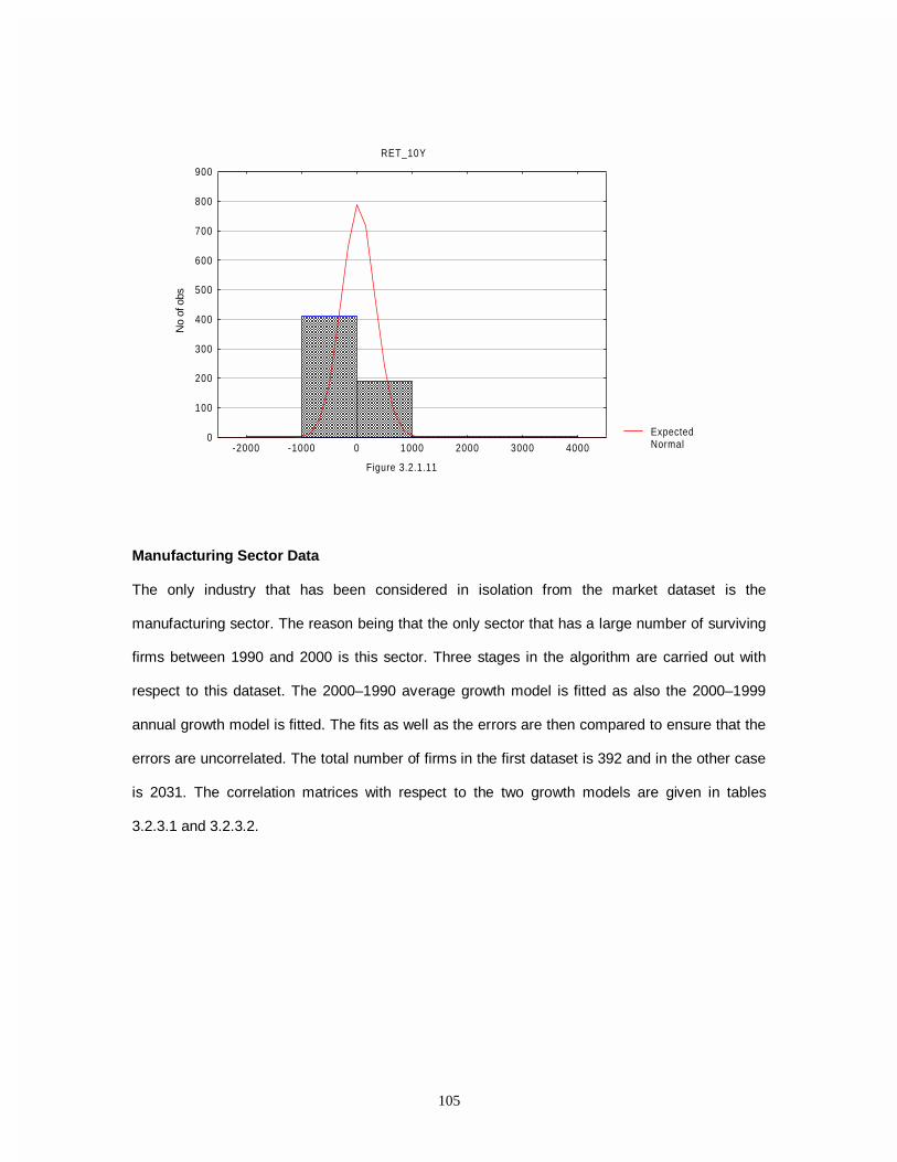
105

Manufacturing Sector Data

The only industry that has been considered in isolation from the market dataset is the

manufacturing sector. The reason being that the only sector that has a large number of surviving

firms between 1990 and 2000 is this sector. Three stages in the algorithm are carried out with

respect to this dataset. The 2000–1990 average growth model is fitted as also the 2000–1999

annual growth model is fitted. The fits as well as the errors are then compared to ensure that the

errors are uncorrelated. The total number of firms in the first dataset is 392 and in the other case

is 2031. The correlation matrices with respect to the two growth models are given in tables

3.2.3.1 and 3.2.3.2.

ExpectedNormal

RET_10Y

Figure 3.2.1.11

No

of o

bs

0

100

200

300

400

500

600

700

800

900

-2000 -1000 0 1000 2000 3000 4000

106

NW_SH90 DE_SH90 PI_SH90 IC_SH90 DIV_SH90 GNW_ S10Y

GDE_ S10Y

GPT_ S10Y

GDV_ S10Y

GIC_ S10Y

RET10Y

NW_SH90 1.00 .02 .81* .43* .84* -1.00* -.03 -.42* -.51* -.22* .22*

DE_SH90 .02 1.00 -.01 -.03 .00 -.02 -.73* .03 .01 .03 .01

PI_SH90 .81* -.01 1.00 .70* .72* -.81* -.01 -.59* -.39* -.30* .31*

IC_SH90 .43* -.03 .70* 1.00 .39* -.42* .03 -.43* -.13* -.29* .36*

DIV_SH90 .84* .00 .72* .39* 1.00 -.84* -.01 -.54* -.68* -.28* .10

GNW_S10Y -1.00* -.02 -.81* -.42* -.84* 1.00 .10 .42* .51* .22* -.22*

GDE_S10Y -.03 -.73* -.01 .03 -.01 .10 1.00 -.00 -.01 -.02 -.02

GPT_S10Y -.42* .03 -.59* -.43* -.54* .42* -.00 1.00 .61* .22* .21*

GDV_S10Y -.51* .01 -.39* -.13* -.68* .51* -.01 .61* 1.00 .30* .41*

GIC_SH10Y -.22* .03 -.30* -.29* -.28* .22* -.02 .22* .30* 1.00 .05

RET10Y .22* .01 .31* .36* .10 -.22* -.02 .21* .41* .05 1.00

*Marked correlations are significant at p < .05000 N=392

7DEOH �������

107

NW_SH90 DE_SH90

PI_SH90 IC_SH90 DIV_SH90 GNW _S1Y

GDE _S1Y

GPT _S1Y

GDV _S1Y

GIC _SH1Y

RET1Y

NW_SH90 1.00 .01 .69* .24* .42* .43* -.00 .24* -.01 .14* -.21*

DE_SH90 .01 1.00 .02 .00 -.00 .01 -.34* -.00 .00 -.01 .00

PI_SH90 .69* .02 1.00 .47* .46* .31* -.01 -.27* -.01 .03 -.22*

IC_SH90 .24* .00 .47* 1.00 .32* -.30* .00 -.11* .01 .38* -.12*

DIV_SH90 .42* -.00 .46* .32* 1.00 .04 -.00 -.09* -.56* -.05* -.38*

GNW_S1Y

.43* .01 .31* -.30* .04 1.00 -.01 .43* .27* -.13* -.10*

GDE_S1Y -.00 -.34* -.01 .00 -.00 -.01 1.00 .00 -.00 .01 .00

GPT_S1Y .24* -.00 -.27* -.11* -.09* .43* .00 1.00 .19* .13* .10*

GDV_S1Y -.01 .00 -.01 .01 -.56* .27* -.00 .19* 1.00 .09* -.02

GIC_SH1Y

.14* -.01 .03 .38* -.05* -.13* .01 .13* .09* 1.00 .10*

RET1Y -.21* .00 -.22* -.12* -.38* -.10* .00 .10* -.02 .10* 1.00

* Marked correlations are significant at p < 0.05 N=2031

7DEOH �������

108

5.3. TIME SERIES MODEL

We consider the following time series model for dynamic price formation in Indian Stock Markets.

Pt+1 Pt = At +B1t NWt + B2t DEt + B3t PIt + B4t DIVt + B5tICt

B6t Et û 1:t + B7t Et û '(t + B8t Et û 3,t + B9t Et û ',9t + B10t Et ¨ ,&t

+ κ~ t , κ~ t ∼ 1 ��� 1

2Kt

)

where, Pt = closing price of shares at 31st December of the year t,

NWt = Net worth per outstanding equity share at 31st December of the year t,

PIt = Profit for the year t after adding back the interest cost, per outstanding equity

share at 31st December of the year t,

DEt = Debt-Equity ratio at 31st December of the year t,

DIVt = Dividend declared during year t per outstanding equity share at 31st December of

the year t,

ICt = Interest cost for the year t,

û 1:t = NWt +1 - NWt , is the first forward difference in NW,

û 3,t = PIt +1 - PIt , is the first forward difference in PI,

û '(t = DEt +1 - DEt, is the first forward difference in DE

û ',9t = DIVt +1 - DIVt is the first forward difference in DIV

¨ ,&t = ICt+1 – ICt is the first forward difference in IC,

Et is the forward looking Rational Expectations operator with respect to 31st December of year t

κ t is a random error term normally distributed with mean 0 and variance matrix 1 � t

2 >0

We shall jointly test for the fit of the model as well as the properties of the error terms

hypothesized, with annual data over the period 1990-2000.

109

The econometric testing of a time series model of this form, which consists of a large cross–

section of companies at any given t can be carried out along two directions. The first method is

the traditional Vector Auto Regression method of the Box–Jenkins type. In such a method the

entire panel data pooled across firms and time periods has to be studied in integrated form to

give GLS estimates by this ARIMA model. This has the potential dimensionality cost of there

being around 2500 firms for each of the years 1990–2000 with twelve variables, which could

potentially become a 2500 X 10 X 12 matrix requiring high computing time and memory costs.

Besides, with a linear model specification such as ours, the nonlinearity involved in the historical

behavior of stock prices would not be readily evident till we change our specification and fit a

nonlinear model all over again. This prompts us to carry out the Time Series GLS regression in a

“nested” procedure similar in many respects with that suggested by Granger & Newbold (1977)

and consists of the following algorithm. This algorithm uses the residual matrix of nested models

to set up an objective function based on correlations amongst the nested residuals. While this

procedure helps in time series estimation of the parameters along the Granger et. al. approach, it

also provides a procedure for estimating TVP (Time Varying Parameter) problems as discussed

in Rao (2000), without using any exogenous cost minimisation objectives.

In the first step we break up the pooled time series ARIMA model into nested models identified by

years as follows:

[ Pt+1 - Pt ] = [ At + ∑=

5

1iitB historical variable it + ∑

=

10

6iitB expectation variable it + κ t]

C ⊗ T

where C is the number of companies in the data set T is the time “ horizon” which in this case is

1990-2000. Bit is the coefficient on historical variable i at time t where i is the indicator as follows:

i=1 ⇒ NW

i=2 ⇒ DE

110

i=3 ⇒ PI

i=4 ⇒ DIV

i=5 ⇒ IC

The historical variables are, as given above, the expectation variables follow exactly the same

identification, i.e.,

i=6 ⇒ Et û 1:

i=7 ⇒ Et û '(

i=8 ⇒ Et û 3,

i=9 ⇒ Et û ',9

I=10 ⇒ Et ¨ ,&

This is the basic time series model.

In the second step, we break up this general ARIMA (1,1,1) specification into first a “bootstrap”

average growth model as follows:

P2000 – P1990 = A + B1 NW1990 + B2 DE1990 + B3 PI1990 + B4 DIV1990 + B5IC1990 + B6 E1990 û 1:2000-1990

+ B7 E1990 û '( 2000-1990 + B8 E1990 û3, 2000-1990 + B9 E1990 û',92000-1990

+ B10E1990 ¨ ,&2000-1990 + κ~

where, E1990 û1:2000-1990 = NW2000 - NW1990 ,

E1990 û'(2000-1990 = DE2000 - DE1990,

E1990 û3,2000-1990 = PI2000 - PI1990

E1990 û',92000-1990 = DIV2000 - DIV1990

E1990 û,&2000-1990 = IC2000 - IC1990

Thus, here the dependent variable is the total price differential over the decade. Any of the

coefficients B6 to B10 is the "average growth" coefficient in the sense that

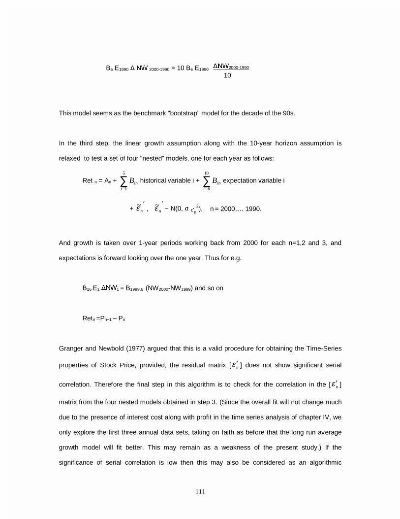
111

B6 E1990 û 1: 2000-1990 = 10 B6 E1990 û1:2000-1990

10

This model seems as the benchmark "bootstrap" model for the decade of the 90s.

In the third step, the linear growth assumption along with the 10-year horizon assumption is

relaxed to test a set of four "nested" models, one for each year as follows:

Ret n = An + ∑=

5

1iinB historical variable i + ∑

=

10

6iinB expectation variable i

+ ′

nε~ , ′

nε~ ~ N(0, 1 0¶n

2), n = 2000…. 1990.

And growth is taken over 1-year periods working back from 2000 for each n=1,2 and 3, and

expectations is forward looking over the one year. Thus for e.g.

B16 E1 û1:1 = B1999,6

(NW2000-NW1999) and so on

Retn =Pn+1 – Pn

Granger and Newbold (1977) argued that this is a valid procedure for obtaining the Time-Series

properties of Stock Price, provided, the residual matrix [ nε ′ ] does not show significant serial

correlation. Therefore the final step in this algorithm is to check for the correlation in the [ nε ′ ]

matrix from the four nested models obtained in step 3. (Since the overall fit will not change much

due to the presence of interest cost along with profit in the time series analysis of chapter IV, we

only explore the first three annual data sets, taking on faith as before that the long run average

growth model will fit better. This may remain as a weakness of the present study.) If the

significance of serial correlation is low then this may also be considered as an algorithmic

112

procedure for cointegration of stock price variables. We test these hypotheses in the following

sections.

5.4. TIME SERIES RESULTS (GOODNESS - OF - FIT)

The "Average Growth " Model

The average growth model for the ten-year period 2000-1990 is presented. The dataset consists

of the entire market data and the partitioned manufacturing data. Both the set of results serve as

a bootstrapping benchmark for the linear model specification in the stage one of the modeling

algorithm.

The Market Data

The total number of "surviving" firms between the decade of 31.12.90 and 31.12.2000 is 571 in

the total market dataset. The average growth model was run on the set taking annual series as

has been discussed before. The results are summarised in the following table:

Variable B t (571) Level of

significance

Intercept

NW1990

DE1990

PI1990

IC1990

DIV1990

GNW2000-1990

GDE2000-1990

-12.69

-0.688

-0.156

6.088

-1.659

10.044

-0.615

-0.204

-1.15

-5.103

-0.168

9.804

-2.88

3.211

-7.46

-0.284

Insignificant

0%

Insignificant

0%

1%

1%

0%

Insignificant

113

GPI2000-1990

GDV2000-1990

GIC2000-1990

4.762

18.407

-1.092

10.209

8.157

-2.245

0%

0%

3%

Thus, the estimated equation becomes:

P2000 - P1990 = -12.69 - 0.688 NW1990 - 0.156 DE1990 + 6.088 PI1990 - 1.659 IC1990 + 10.04 DIV1990

(-1.15) (-5.103) (-0.168) (9.804) (-2.88) (3.211)

-0.615 GNW2000-1990 - 0.204 GDE2000-1990 + 4.762 GPI2000-1990 + 18.407 GDV2000-1990

(-7.46) (-0.284) (10.209) (8.157)

- 1.092 GIC2000-1990

(-2.245)

The R2 is high at 0.52 and the F-statistic is high at 63.36 which is significant at the 0% level and

the serial correlation of the residuals is low at 0.08 suggesting a good fit for the model. In fact, the

fit of the model improves significantly with the inclusion of the interest cost separately.

The significant weights on the initial net worth (NW1990), initial profit (PI1990), initial interest cost

(IC1990), initial dividend (DIV1990), and in their growth is substantiated by the model, while the signs

of the coefficients are suggestive of the predominance of the supply or demand factors over the

other, as the case may be. The fitted "price differential" line is plotted in fig. 3.4.1.1 as Ret 10Y.

114

Regression95% confid.

Predicted vs. Observed Values

Dependent variable: RET_10Y

Figure 3.4.1.1

Predicted Values

Obs

erve

d V

alue

s

-1500

-500

500

1500

2500

3500

4500

-1000 0 1000 2000 3000 4000

115

Manufacturing Sector Data

The total number of "surviving " firms in the manufacturing sector dataset over the period 2000 -

1990 is 392. The average growth linear model was run on the data set taking annual series, as

has been discussed, to obtain the GLS estimates. The results are presented in the following

table:

Variable B t (381) Level of

significance

Intercept

NW1990

DE1990

PI1990

IC1990

DIV1990

GNW2000-1990

GDE2000-1990

GPI2000-1990

GDV2000-1990

GIC2000-1990

-49.98

3.75

-3.89

2.691

2.184

25.5

3.81

-4.04

1.96

35.35

0.61

-2.17

0.0

-0.0

3.95

3.75

4.91

0.0

-0.0

5.7

10.59

1.57

4%

Insignificant

Insignificant

1%

1%

1%

Insignificant

Insignificant

0%

0%

Insignificant

The R2 is high at 0.53.

116

The graph of the plot of the fitted price differential is shown in figure 3.4.1.2.

Annual Price Differential Data

In keeping with the algorithmic approach to the time series analysis of this paper we regress the

model on annual data for the periods 2000-1997. We only consider three annual data as they

comprise the most recent three years and extrapolate our results on the basis of the results

obtained in this section as well as chapter IV. The results of the regression for the various periods

within the decade are summarized in the following table 3.4.1.3.1.

Regression95% confid.

Predicted vs. Observed Values

Dependent variable: RET_10Y

Figure 3.4.1.2

Predicted Values

Obs

erve

d V

alue

s

-2000

0

2000

4000

6000

8000

-2000 -1000 0 1000 2000 3000 4000 5000 6000

117

Period 00-99 99-98 98-97

Intercept -3.12 (-1.11)

22.83 (5.76)

3.76 (4.24)

NW -0.07 (-2.92)

0.07 (1.91)

0.02 (3.56)

DE 0.02 (0.15)

-0.06 (-0.16)

-0.001 (-0.01)

PI 0.87 (5.79)

1.09 (7.33)

0.123 (2.35)

IC -0.73 (-4.45)

-0.94 (-6.16)

-0.33 (-5.37)

DIV -18.12 (-20.79)

7.04 (6.24)

-2.23 (-7.31)

GNW -0.51 (-5.47)

0.25 (3.92)

-0.32 (-7.49)

GDE 0.006 (0.08)

-0.05 (-0.25)

0.00 (0.09)

GPI 1.42 (8.23)

1.16 (6.37)

0.58 (7.28)

GDV -14.36 (-12.25)

6.91 (5.40)

1.39 (4.42)

GIC 0.42 (1.41)

-1.78 (-6.27)

-0.64 (-6.75)

R2 0.21 0.09 0.09

F 71.21 28.84 35.68

DW 1.84 1.76 1.98

7DEOH ���������

118

The fit of the three annual models never perform better than the average growth model over the

10-year horizon, in terms of R2, which has a significantly high R2 at 0.52. Besides the F statistic is

significant for the average growth rational expectations model over 10 years and the serial

correlation of residuals is also low, rejecting a nonlinear fit to the pricing equation through annual

series in favour of a linear fit, as was the case in Chapter IV. This inference is correct based on

the comparison of the two sets of models, because as required by Granger & Newbold (1977),

the error correlation matrix among the nested residuals shown in table 3.4.1.3.2 do not show

significant serial correlation.

Table 3.4.1.3.2

E1 E2

E3

E1 1.00 -0.09* -0.00 E2 -0.09* 1.00 0.01 E3 -0.00 0.01 1.00 Marked correlations are significant at p < 0.05000

This rejects the hypothesis of significant correlation, as the maximum magnitude is 0.09. This

inference is also true when one compares the manufacturing sector for its fit over 2000-1990 with

2000-1999 the most recent one year. The results for the 2000-1999 period are given in table

3.4.1.3.3.

119

Table 3.4.1.3.3

Variable B t statistic

(2020)

Level of significance

Intercept

NW99

DE99

PI99

IC99

DIV99

GNW

GDE

GPT

GDV

GIC

-1.69

-0.21

0.01

1.83

-0.85

-22.12

-0.6

0.002

2.31

-20.46

1.95

-0.49

-6.57

0.04

8.7

-3.84

-20.84

-5.29

0.03

10.05

-14.49

4.45

Insignificant

0%

Insignificant

0%

1%

0%

0%

Insignificant

0%

0%

1%

Adjusted R2 is 0.27

Here also the average growth ten-year model obtains a better fit, suggesting that the longer term

linear rational expectations model performs better. In other words the cointegrated price variables

fit better in both cases with a linear average growth trend. Both these observations are somewhat

incongruous with a high and significant weightage on historical dividends and dividend growths,

which suggest high liquidity preference and therefore "myopia". Associated with this, is a

significant positive sensitivity of returns with interest cost, both in levels as well as in growth.

Positive elasticity with interest cost suggests that demand effect for manufacturing shares is

outweighed by the supply effect (Tobin (1972) for example). This implies that the monetary

authority, by adjusting the interest rate, can have a significant positive effect on returns in

120

manufacturing shares. This is true whether the annual 2000-1999 dataset is being discussed or

the average growth 10-year 2000-1990 dataset is being considered.

The fitted lines for the ten-year average growth model and for the 2000-1999 model for the entire

market dataset are presented in figures 3.4.1.3.4 and 3.4.1.3.5.

5.5. TIME SERIES RESULTS (VOLATILITY)

Regression95% confid.

Predicted vs. Observed Values

Dependent variable: RET_10Y

Figure 3.4.1.3.4

Predicted Values

Obs

erve

d V

alue

s

-1500

-500

500

1500

2500

3500

4500

-1000 0 1000 2000 3000 4000

Regression95% confid.

Predicted vs. Observed Values

Dependent variable: RET_1Y

Figure 3.4.1.3.5

Predicted Values

Obs

erve

d V

alue

s

-3500

-2500

-1500

-500

500

1500

2500

-2000 -1600 -1200 -800 -400 0 400 800

121

An analysis of fit of the model to the time series data reveals that, on average a good part of the

dynamic price differential is explained by the set of historical and rational expectations variables

considered, giving an overall R2 (adjusted for serial autocorrelation and heteroskedasticity) of

0.52 with significant t-statistic on all but the debt-equity variables. The fit of the model in the case

of the benchmark set of companies, having market price/face value ratio >=10 (consisting of 93

companies), is significantly higher with an adjusted R2 = 0.77 and significant t-statistic for all but

the interest cost and dividend variables. The fit of the model is also striking in the case of the

manufacturing sector with an adjusted R2 of 0.53. However, it still leaves a lot of volatility to be

explained.

When it comes to an analysis of the volatility in the residuals it is observed that as was true in the

case with no interest cost variable, the F-statistic and DW-statistic are both significantly high,

leaving therefore the variance to be analysed only (in the general dataset, F = 63.36 and DW=

1.83; in the benchmark dataset, F = 30.99 and DW= 2.02; and in the manufacturing sector data

set, F = 44.69 and DW= 1.93). Further an analysis of the correlation matrix across the various

"nested " models of annual duration suggest that the across period serial correlations are

insignificant. This not only points to the existence of a ten-year set of data cointegrated with the

price differentials but also to the fact that residuals follow "random walk" over time at least within

this ten-year history. However, after the conditioning on the variables of the model, including the

monetary policy variables of interest cost and growth in interest cost, the errors do follow a

"random walk" pattern. The reduction in residual variance consequent to the treatment of the

interest cost variable in terms of increase in R2 over the ten-year dataset are given in the

following table.

122

Adjusted R2 without

monetary policy variables

Adjusted R2 with monetary

policy variables

Total Market 0.36 0.52

Benchmark Data Set 0.62 0.77

Manufacturing 0.46 0.53

It has already been noted in previous chapters that "myopia" through dividend and expected

dividend dependence operates in contrast to the overriding performance of the longer-term

average growth model, which is an anomaly found in this study. However, the significant variance

of the residual sum of squares does certainly point direction to speculative "gambling" and

"sunspot" components in the stock market. The elasticities of the variances in returns as is

captured by the B coefficients in the regression equations are given below for the three datasets

in the ten-year average growth model.

B for Interest Cost B for Growth in Interest Cost

Total Market -1.66

(2.88)

-1.09

(-2.24)

Benchmark Data Set 4.21

(1.11 - insignificant)

8.95

(2.41)

Manufacturing 2.18

(3.95)

0.61

(1.57 – insignificant)

Thus, the variability reducing power of the interest variables in all the above three categories of

industries is corroborated by the significance of at least one t-statistic in all the cases (as

originally suggested in, for example, the Tobin (1972) paper). However, the signs and magnitudes

of the coefficients are not uniform even within this ten-year time series analysis. In the overall

market data, the Bs lie between 1 and 2 with negative signs. Since interest rates and therefore

interest costs are profit-reducing elements for companies, hence, the demand side of the capital

123

market ought to be negatively related to interest (law of demand). On the other hand, supply of

capital ought to have a positive relation with interest by savings theories. Hence, a negative net

effect on price differentials suggests that the demand for capital (supply of shares) effect

dominates the supply of capital (demand for shares) effect.

5.6 CONCLUSION

From our discussions above, it can be discerned that, in the case of major blue chip companies,

pursual of a “cheap money” policy by the Reserve Bank of India may lead to an increase in the

net demand for capital thereby increasing returns on capital through the stock market.

However, other classifications of company groupings do not result in similar observations. In

these cases, the supply side of the capital market (i.e. the demand side of the share market)

dominates the demand side as it is reflected in a positive interest sensitivity. In more specific

terms, as interest (cost) increases, the supply of capital increases as savings increases, part of

which is mobilised by financial institutions and channelised into equity markets, leading to

increase in demand for shares, resulting in increase in share prices and thus returns.

Alternatively, another possible explanation for this may be derived from the positive income effect

on demand for shares derived from increase in interest income to savers and the resultant

upward pull on share prices resulting from the demand increase. However, on average interest

income constitutes a much smaller portion of the income of financial institutions (who are the

major investors) compared to income from securities, dividends and capital gains. Hence, this

marked shift in the signs of the coefficients is somewhat anomalous, pointing to a possible

presence of short-term myopia exacerbating fragility, requiring further in-depth study.

124

CHAPTER VI ªÉ

FINANCIAL FRAGILITY IN THE BANKING SECTOR: A TIME SERIES ANALYSIS OF NON-PERFORMING ASSETS

6.1 INTRODUCTION

The beneficial impact of a well functioning financial system, particularly the banking sector, on the

real sector is well known. As such, the existence or lack of fragility or vulnerability or “proneness”

to random shocks or unforeseen events assumes a critical dimension. Allen and Gayle (2000),

Kaminsky and Reinhart (1999, 1996), Kiyotaki and Moore (1997), Rakshit (1998), Stiglitz (1981)

and others have examined the factors that make the banking sector particularly fragile. The

existing literature has expressed concern over the inherent tendencies in the banking sector

towards fragility, arising out of institutional characteristics with respect to norms / rules and

inadequate controls. We discuss a combination of macroeconomic, microeconomic and

rules/norms based factors – all contributing to this fragility of the banking system. Further, our

study and empirical analysis brings out three significant tendencies. First, NPAs (as a ratio of

loans and advances) are significantly sticky over time. Second, larger NPAs are associated with

larger advances and vice-versa; and third, NPAs do not seem to be spiraling out of control, rather

shows signs of a slight reduction. The policy initiated during the 90s of classifying bad debts as

NPAs after two installment defaults, seems to have brought some amount of control on the bad

debts situation. However, this study also shows that the real and asymmetric information

problems associated with bad debts formation needs serious attention.

On the macroeconomic side there are national economy wide and even global economy wide

factors, which are essentially beyond the control of the banking sector or individual banks. Large

cyclical fluctuations in the level of economic activity, high and variable inflation and interest rates,

large and unforeseen shocks in world demand and supply conditions of the country’s exportables

125

and importables, volatility in foreign exchange and capital markets raise the degree of risk to be

confronted by producers (borrowers) and hence by banks (and lenders) as well. The macro-

impact becomes more critical in less developed economies with relatively undeveloped stock

markets and where, as such, firms are compelled to resort to borrowings.

On the microeconomic side, there are several factors that tend to make the system “inherently”

fragile. There is the major problem of collecting information pertaining to the solvency of the bank,

which in turn depends on the solvency and creditworthiness of the borrowers. Depositors

generally have very little means or ability to monitor the activities of the banks or to judge the

quality of the bank assets. Further, there is the inherent distortion under little or no regulation of

the banking sector resulting in the high ratio of deposits to own funds of banks; and as we know

under the law of limited liability total loss of banks cannot exceed their own funds invested.

These factors result in two types of distortion in banking, viz., adverse selection and moral

hazard. As Akerlof and Roemer (1993) have pointed out, the difficulty of monitoring the activity of

banks by depositors and control over large funds of which bankers themselves own a small

fraction put great temptation in their own way to indulge in shady deals for personal gains and

siphon off bank’s resources.

Further, as Rakshit (1998) has demonstrated, under the free play of market forces, banks

inherently tend to choose (a) projects that are high risk and have low expected returns; and (b)

the deposit rate tends to exceed the expected return on the projects chosen. Even when banks

are risk averse, banks’ management of risk, when left to themselves, tend to be both inadequate

and inefficient.

Further, we have observed in all too many instances, an inherent tendency for troubles specific to

individual banks, leads to serious contagion and precipitate a sector-wide and systemic crisis.

126

Hence, there is a need for public intervention (regulation or supervision) in banking at both the

macro and micro levels.

In addition to basic contra-cyclical macro-stabilisation policies (which alone cannot do away the

fragility of the banking sector), one suggested way out for averting run on banks and systematic

crisis in the banking sector is deposit insurance or some form of government guarantee.

However, it is widely held that such measures create and compound serious moral hazard

problems by way of inducing bankers to finance high risk projects and removing all incentives for

depositors to gather necessary information, monitor bank’s activities and assess bank’s

performance.

This highlights the importance of effective bank regulation and supervision for ensuring the

viability of the banking sector. One such step towards regulation involves restricting competition,

as discussed in Caprio and Summers (1998), through some form of licensing (scrutinizing record

of applicants seeking entry into the banking sector) – thus ‘preventing entry of entrepreneurs’ of

doubtful ability and integrity. Another measure or instrument of regulation will be to administer the

own capital to total investment ratio, though there is a clear dilemma in the exercise of this

instrument for regulation of banks. As Rakshit (1998) has shown, a low own-capital ratio tends to

undermine viability of the banking sector through gross distortion in bank’s choice of assets; on

the other hand, fixing the ratio at a very high level severely limits the financial intermediation,

especially in a developing economy.

Although attainment and maintenance of macroeconomic stability is necessary for avoiding

financial crisis, the task of attaining macro balance is frequently seen to be beyond the capability

of many a country. As Rakshit (1998) has shown, with the lack of built-in flexibility of the tax

system particularly in a developing economy and the difficulty of counter-cyclical adjustment of

normal government expenditure, it is argued that macro-stabilisation may require public debt

backed by public assets in commercially run enterprises. Monetary measures being flexible are

127

more effective than fiscal measures, in the short run, in countering cyclical fluctuations, though

mobility of international capital has put serious constraints on the policy options before the

Central Bank.

In such contexts, the need for adequate regulation and effective supervision of banks becomes

paramount. The Bank of International Settlement (BIS) has been engaged in developing

appropriate norms to be observed by banks and formulating principles for their regulation. The

recommendations of both the 1991 and 1998 Narasimhan Committee (Reserve Bank of India) are

primarily based on successive reports of the Bank Committee on Banking Supervision, that are

set up by the BIS. The “core principles” set forth in the 1997 Basle Committee report (BIS, 1997)

constitute the minimum requirements for effective banking supervision, licensing, prudential

requirements, information requirements and cross border banking. The Basle Committee report

recommends necessary supplements by other measures in the context of specific conditions and

risks in the financial system of particular countries. For example, prudential requirements relate to

capital adequacy, asset quality and related provisioning norms, asset liability management and

accurate accounting. The most crucial of the prudential norms is capital adequacy which under

the Basle Capital Accord of 1988 is set in terms of a minimum Capital to Risk Assets Ratio

(CRAR) of a bank, set at 8%. The Narasimhan Committee had recommended that Indian Banks

should attain a minimum CRAR of 9% by the year 2000 and 10% by the year 2002.

However, there are at least two major limitations of the capital adequacy and related norms. In

the first place, in the context of the observations made above, the norms on their own are quite

inadequate in preventing moral hazard. Secondly, as discussed in Rakshit (1998), they tend to

produce macro-instability (and thus fragility or vulnerability) both through pro-cyclical behaviour of

credit and changes in its composition during the course of the cycle. During the upward phase of

the cycle, there is rapid increase in the capital base of the banks with accumulation of reserves

out of profits boosted through (a) booming business conditions, and (b) sharp fall in provisioning

requirements with improvement in quality of bank assets and a decline in NPAs. The result is

128

sharp growth in bank credit, while macro-stabilisation requires its containment during this period.

Similarly, it can be shown that the Basle norms will add to the credit crunch during a depression.

Finally, it is also important to recognise and give effect to inherent interrelationships between

regulatory measures and monetary policies so as to ensure proper coordination of the two types

of policies towards achievement of stability in the financial sector in general and the banking

sector in particular.

The organisation of this chapter is as follows. In section 6.2 we discuss the outline of the model

used for analysis. In section 6.3 we discuss the dataset. In section 6.4 we provide a time series

ARIMA (1,0,1) Maximum Likelihood analysis and the results. In section 6.5 we conclude.

6.2 THE MODEL

The banking sector in India, since the nationalisation in the late 60’s and early 80’s, is largely

state-owned in the form of nationalised banks. Since, till recently, shares of nationalised banks

were not traded in the stock market, financial performance of banks is to be measured with

respect to criteria different from that of companies listed on the stock exchange and as discussed

in the previous chapters. Besides, banking companies being financial institutions, belong to a

different industrial sector and hence measures of performance have to differ. Such discussions

can be traced to the literature on the economics of banking in such papers as Gurley and Shaw

(1960), Rakshit (1998), Bagchi (1998).

The purpose of this study, in keeping with the overall purpose of this project, is to assess the

extent of financial fragility in the banking system over the period covering the 1980s and the

1990s. This period has witnessed the significant structural change involving the opening up of the

stock markets and the trading of portions of shares of certain nationalised banks notably the State

Bank of India, in the stock market. However, since the significant nature of operations of the

banks remains the inflow and outflow of credit through the mechanism of interest rates (i.e.

129

commercial banking), therefore financial performance of banks have to be measured in terms of

the efficient intake and maturity of deposits and efficient provision and recovery of loans and

advances. The two essential variables in this circulation mechanism are interest and bad debts.

Interest received on loans and advances forms the major part of the income of the banking

sector, while interest paid and bad debts (technically renamed as non-performing assets) forms

the major part of the costs of the banking sector. On comparison of the nationalised as opposed

to private banks, as will be discussed in the data section in detail, it is evident that NPA forms a

formidable problem for the nationalised banks as opposed to private banks. However, since

nationalised banks constitute a majority portion of the banking sector’s total deposits as well as

loans and advances, because of its historical priority on small savings and prioritised lending,

NPA forms a significant cost to the efficient functioning of the banking sector as a whole and the

key factor in the financial fragility of the banking system.

Explanations for the level of NPAs are not hard to find. To a large extent, as is the case with any

industry, bad debts arise due to an inefficient system of management and recovery of debt along

with the real economic causes of business failure. When applied to the banking sector, lending

gets coupled with bad debts as possible explanations for the incidence of NPA costs. Thus,

lending to bad quality projects both in terms of technology and risk, asymmetric information giving

rise to imperfect screening and monitoring which results in adverse selection of projects and

terms of lending, and moral hazard in the monitoring and recovery of loans (Stiglitz & Weiss

(1981)), lead to the large incidence of NPA costs. According to the definition of NPA given by the

Reserve Bank of India, non-performing assets are those loans and advances on which interest

payment is in default for more than two quarters. Hence, it includes not only bad debts but also

other loans and advances which fall in the risky category with respect to debt servicing. Thus, the

broad definition of risk assets in the adverse selection and moral hazard literature coincides more

or less with the NPA definition.

130

An interpretation of the asymmetric information literature as discussed above, can proceed as

follows. Banks, which had lent in the past to high default risk category of firms due to priority

reasons or the adverse selection and moral hazard reasons, find it difficult to recover interest

income as well as the principal. This reduces the debt-service-coverage-ratio of bank deposits

inducing thereby to lend to higher return higher risk category of customers. This, due to the

dynamic operation of the adverse selection and moral hazard problems, accumulates further

NPAs. By this argument, the aggregate implication is that, “NPAs give rise to further NPAs” in the

Indian banking sector. In this chapter, we pursue this line of reasoning to test the time series

properties of NPAs. Hence, as will be seen, NPAs expressed as a function of outstanding loans

and advances are self-driven over time and this stickiness has given rise to a vicious cycle of bad

debts in the banking sector, which makes the entire financial system fragile by impeding the

operation of the multiplier.

6.3 THE DATASET

The dataset comprises the period 1995–2000 for which full data is available in the Prowess

database of the Centre for Monitoring the Indian Economy, and consists of a maximum of 188

banking companies in 1998 and a minimum of 121 banking companies in 1995. The variables

that are considered for the purpose of the present study are as follows: provision for bad debts

(NPA) for the year, closing balance of loans and advances, and the year of operation. With these

variables, we construct a composite variable 100 * bad debts / loans & advances = ratio_p to

express bad debts as a function of loans and advances. As has been already discussed in the

previous section, bad debts and NPAs will be used interchangeably. The graphs of the variables

are given below. Figure 6.1 describes the plot of the Bad Debts (NPAs) over time ranging from

first half of 1995 to second half of 2000. Figure 6.2 describes the plot of the NPA to loans and

advances ratio (ratio_p) over time. Figure 6.3 describes the plot of Bad Debts against advances.

This shows a significant clustering at small advances and low bad debt levels. Besides, there

131

seems to be a linear trend that we estimate in the next section. Figure 6.4 describes the plot of

ratio_p against advances. This again shows a significant clustering close to the origin. Besides,

there seems to be a constant relation across level of advances. Figures 6.5 and 6.6 are three-

dimensional graphs, plotting the Bad Debts and the ratio_p against advances and across time.

While a clear picture does not seem to emerge graphically, a clustering of points at the low

advance - low bad debt and low bad debt - advance ratio levels are clearly discernible. How these

relations change (or remain sticky) over time are analysed in the M-L estimation in the next

section.

Figure 6.1

Figure 6.2

T I M E

BD

EB

TS

- 200

2 0 0

6 0 0

1 0 0 0

1 4 0 0

1 8 0 0

0.5 1 .5 2 .5 3 .5 4 .5 5 .5 6 .5

132

Figure 6.3

Figure 6.4

T I M E

RA

TIO

_P

- 20

2 0

6 0

1 0 0

1 4 0

1 8 0

0.5 1 .5 2 .5 3 .5 4 .5 5 .5 6 .5

A D V A N C E S

BD

EB

TS

- 200

2 0 0

6 0 0

1 0 0 0

1 4 0 0

1 8 0 0

- 1 0 0 0 0 1 0 0 0 0 3 0 0 0 0 5 0 0 0 0 7 0 0 0 0 9 0 0 0 0 1.1e5

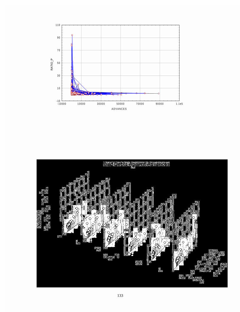
133

A D V A N C E S

RA

TIO

_P

- 10

1 0

3 0

5 0

7 0

9 0

1 1 0

- 1 0 0 0 0 1 0 0 0 0 3 0 0 0 0 5 0 0 0 0 7 0 0 0 0 9 0 0 0 0 1.1e5

134

Figure 6.6

6.4 TIME SERIES RESULTS

The ARIMA (1,0,1) results of the single series (ratio_p) time series are presented in table 6.1. The

ratio_p variable is regressed on itself 1 period lagged and 1 period led. The model is of the

following nature:

ratio_p t = A + B1 ratio_p t-1 + B2 ratio_p t+1 + tε~ , tε~ ~ N(0, 120 t)

The parameters of the model are estimated using maximum likelihood estimation procedure.

135

Table 6.1

Model:(1,0,1) MS Residual=40.730 Asympt. Asympt. Lower Upper Param. Std.Err. t ( 914) p 95% Conf 95% Conf Constant 2.564742* .259974* 9.86537* .000000* 2.054526* 3.074958* p(1) .941871* .063173* 14.90940* 0.000000* .817890* 1.065852* q(1) .928103* .069250* 13.40221* 0.000000* .792195* 1.064010* Marked entries are significant. Table 6.2 Parameter Covariances

Model:(1,0,1) MS Residual=40.730 Constant p(1) q(1) Constant .067587 .004796 .000373 p(1) .004796 .003991 .004306 q(1) .000373 .004306 .004796 Table 6.3 Parameter Correlations

Model: (1,0,1) MS Residual=40.730 Constant p(1) q(1) Constant 1.000000 .291996 .020696 p(1) .291996 1.000000 .984292 q(1) .020696 .984292 1.000000

As was evident from the graphical analysis, the time series shows a significant secular trend and

a significant intercept. The p coefficient (autoregressive) takes on a value of 0.94 and the q

coefficient (autoregressive) is 0.93. Both these estimates are less than 1, thereby predicting

stability in the long run. Besides, the coefficients are close to 1, although decaying slowly at

around 1%. Thus, the ratio of NPA to Total Loans and Advances can be taken to be constant

over the short run. An inference which directly follows is that bigger value of advances are likely

to be associated with bigger default, while smaller advances are less likely to be in default.

There is a significant constant intercept of 2.6, thereby signifying a chronic bad debt problem

which does not change over time and therefore with the volume of advances by the banks. This

requires suitable policy controls. However, the redeeming feature is that, as discussed above, the

series is stable and therefore does not predict immediate signs of spiraling out of control.

The estimated equation obtains as follows:

136

ratio_p t = 2.56 + 0.94 ratio_p t-1 + 0.93 ratio_p t+1

(9.87) (14.91) (13.40)

The graph of the predicted variable for the first 500 cases is given below.

6.5 CONCLUSION

Two significant tendencies emerge from the above analysis. First, NPAs are significantly sticky

over time. Second, larger NPAs are associated with larger advances and vice-versa. However,

optimism can still prevail – NPAs do not seem to be spiraling out of control and shows signs of a

slight reduction. The policy initiated during the 90s of classifying bad debts as NPAs after two

installments’ default, seems to have brought some amount of control on the bad debts situation.

However, whether such a policy, which is more accounting in nature, can address the real

economic problems associated with bank loans going bad is another question. As this study

shows, the real and asymmetric information problems associated with bad debts formation needs

serious attention. Till then, the vicious cycle of NPAs giving rise to further NPAs continues.

Fragility of the banking system, which largely enjoys the insurance of State support due to it being

nationalised to a large extent, is thus more complex than that of the stock market. For, in spite of

Forecasts; Model:(1,0,1)

Input: RATIO_P

Figure 6.7

Observed Forecast ± 90.0000%

-20

0

20

40

60

80

100

120

-20

0

20

40

60

80

100

120

-100 0 100 200 300 400 500 600 700 800 900 1000 1100 1200 1300 1400 1500

137

there being infusion of working capital consequent to nationalisation, mobilisation of savings from

the grassroot level by the safety offered by State guarantee, and a well organised trade union

movement covering the banking sector, the NPA / Advances ratio has observations as high as

90%.

The mean of this ratio is 2.54%, which although is not high in percentage terms, can primarily

translate into two implications. Firstly, since the total advances is Rs. 6,06,151.04 crores in 2000,

the predicted NPA would be around Rs. 15,396 crores, which comes to around Rs. 150 per

capita. This figure is significant if confidence in the banking system is perturbed somehow.

Secondly, since according to the accounting system followed in banks this 2.54% is a charge on

profits, therefore assuming rational decision making in the banking sector, interest rates charged

can be expected to be inflated by at least this figure of 2.54%, which has its own spiraling

depressing effects on growth.

Thus, while policy attention seems to be overtly fixed on the stock market with the globalisation

regime, cumulative effects of history on the operation of the current banking system requires

appropriate attention. This attention probably has to draw upon the interaction of the banking

sector with the real economy as well as the interaction of the banking sector with the stock

market.

138

CHAPTER VII

CONCLUSION AREAS OF FURTHER RESEARCH

In conclusion, our research entitled “Financial Fragility, Asset Bubbles, Capital Structure and Real Rate of

Growth – A Study of the Indian Economy During 1970 –2000” has led us to an in-depth study of critical

relationships, first, between the real and financial sectors, and second, in respect of financial markets in

general and equity markets and the banking sector in particular.

Our analysis clearly reveals that in so far as the financial sector is concerned, the size, activity and

efficiency of the financial intermediaries have improved considerably since financial reforms were adopted.

However, what should be extremely worrying for the reformers is the result showing that the allocation of

credit (savings) is not favouring the private sector. The ratio of government credit to private credit has been

increasing since mid 1990s. With the increasing withdrawal of government from activities in the real sector,

this investment tendency clearly indicates relative inactivity of the private sector in the real economy. The

reason for the relative inactivity of the real sector lies not with the financial sector but probably in problems

pertaining to the real economy supply and demand constraints.

Our cross-sectional study shows conclusively that price formation in Indian Stock Markets is significantly

dependent on net worth of companies as well as their profitability and dividend payouts. However, capital

structure in the form of debt/equity ratio never gets significant weightage although the weightage is

negative. It is also observed that the beta coefficients (B’s) on Net worth per share is negative. This can be

explained by the decomposition of excess demand in that the supply of share capital as well as demand

depends on this variable in opposite ways. Dividend is found to have significant weightage through demand

for share capital. It corroborates both liquidity preference and “short-sightedness" (myopia) amongst the

participants of the Indian stock market. The signaling rationale for dividends is probably rejected due to the

insignificance of Dividends in the case of "blue chip" companies, whereas Net worth and Profit get

139

significant weightage. There seems to be an anomaly with respect to risk perception of participants if debt-

equity ratio and dividend payments are considered side by side for the rest of the data sets.

The estimated equation for the control dataset consisting of the blue chip companies is as follows:

P̂ = 134.367 + 0.603 WN ˆ -10.309 ED ˆ + 6.608 TP ˆ + 4.129 VD ˆ

(3.294) (2.856) (-0.405) (4.638) (0.650)

The estimated equation for the market dataset is as follows:

P̂ = 15.355 +0.1151 WN ˆ -0.007 ED ˆ + 0.519 TP ˆ + 23.632 VD ˆ

(3.394) (2.371) (-0.055) (2.015) (18.850)

The Indian stock market is however significantly described by "bounded rationality", through myopia,

liquidity preference and significant volatility of the error terms when compared within the ratio of

unexplained to total sum of squares. The ratio is reasonably high in all cases, and is significantly high in

some cases, although the power of the model and of the tests is demonstrably high. This leaves a lot of

controls and long run policies with respect to the stock market to be desired.

Side by side with a good explanation of the mean of share prices, is found excess volatility which in most

cases is significant suggesting presence of speculation and non-fundamental driven activities as are

referred to as "sunspots" in the Rational Expectations literature.

The time-series study in respect to the stock market, reveals that the structure of these markets in India is

best described by the presence of historical real (net worth per share, profitability per share ) and financial

(debt-equity ratio, dividend distributed per share ) variables as well as their rationally expected growth

values over the future. This structure is cointegrated with the stock price so that it may be said that in

corporate governance, price is an important consideration in making decisions on the above explanatory

variables at the corporate level. This is in the light of the fact that although there is a lot of residual volatility,

lack of explosive components makes cointegration possible. If one compares it with the fact that the

relationships within the model are stronger in the annual data in periods distant from 1993 and 1997, the

140

two periods of crashes and other significant events, as discussed in the beginning (which therefore opens

up areas of further analysis of structural breaks), then the linear fit, on average, suggests that in spite of a

high degree of volatility, "planned competition" has been responsible in preventing markets from crashing

more often, and changing the overall structure of the interplay between price formation, history and

expectations along with it.

The estimated time series equation incorporating stock prices and growth for the market dataset is as

follows:

P2000 - P1990 = -16.47 - 0.165NW1990 +0.085 DE1990 + 2.819 PT1990 + 23.30 DIV1990

(-1.298) (-1.225) (0.079) (4.33) (6.823)

-2.909 GNW2000-1990 + 0.875 GDE2000-1990 +21.355 GPT2000-1990 + 326.194 GDV2000-1990

(-3.227) (0.106) (4.415) (14.356)

From our inferences drawn from the estimation including macroeconomic variables (interest cost), it can be

discerned that pursual of a “cheap money” policy by the Reserve Bank of India, in the case of major blue

chip companies, may lead to an increase in the net demand for capital, thereby increasing returns on

capital through the stock market.

The estimated time series equation including macroeconomic policy variable for the market dataset is as

follows:

P2000 - P1990 = -12.69 - 0.688 NW1990 - 0.156 DE1990 + 6.088 PI1990 - 1.659 IC1990 + 10.04 DIV1990

(-1.15) (-5.103) (-0.168) (9.804) (-2.88) (3.211)

141

-0.615 GNW2000-1990 - 0.204 GDE2000-1990 + 4.762 GPI2000-1990 + 18.407 GDV2000-1990

(-7.46) (-0.284) (10.209) (8.157)

- 1.092 GIC2000-1990

(-2.245)

However, other classifications of company groupings do not result in similar observations. In these cases,

the supply side of the capital market (i.e. the demand side of the share market) dominates the demand side

as it is reflected in a positive interest sensitivity. In more specific terms, as interest (cost) increases, the

supply of capital increases as savings increases, part of which is mobilised by financial institutions and

channelised into equity markets, leading to increase in demand for shares, resulting in increase in share

prices and thus returns. Alternatively, another possible explanation for this may be derived from the positive

income effect on demand for shares derived from increase in interest income to savers and the resultant

upward pull on share prices resulting from the demand increase. However, on average, interest income

constitutes a much smaller portion of the income of financial institutions (who are the major investors)

compared to income from securities, dividends and capital gains. Hence, this marked shift in the signs of

the coefficients is somewhat anomalous, pointing to a possible presence of short-term myopia exacerbating

fragility requiring further in-depth study.

The existing literature has expressed concern over the inherent tendencies in the banking sector towards

fragility, arising out of institutional characteristics with respect to norms / rules and inadequate controls. Our

study and empirical analysis brings out three significant tendencies. First, NPAs (as a ratio of loans and

advances) are significantly sticky over time. Second, larger NPAs are associated with larger advances and

vice-versa; and third, NPAs do not seem to be spiraling out of control, rather shows signs of a slight

reduction. The policy initiated during the 90s of classifying bad debts as NPAs after two installment defaults,

seems to have brought some amount of control on the bad debts situation. However, this study also shows

that the real and asymmetric information problems associated with bad debts formation needs serious

attention.

142

The Maximum Likelihood estimated time series equation for the banking sector data set is as follows:

ratio_p t = 2.56 + 0.94 ratio_p t-1 + 0.93 ratio_p t+1

(9.87) (14.91) (13.40)

As we have observed, solvency of banks may be threatened by the factors operating at both the global and

national wide levels. The existing literature has highlighted the institutional aspects of the financial fragility

in the banking sector with a look into the efficacy of Bank for International Settlements (BIS) norms and

other policy programmes in reducing financial fragility. There is, however, need and scope for a

comprehensive fundamentals–based analysis of the fragility in the banking sector.

With the collapse of the Bretton-Woods fixed exchange rate system and introduction of freely floating

exchange rates from 1973 practically by all industrialised countries, it was observed that exchange rates

exhibited considerable volatility and prolonged periods of overvaluation and undervaluation in both size and

duration, all indicating currency markets not being satisfactorily determined by fundamentals leading to

financial fragility in such markets.

In case of India, the switch to a floating exchange rate regime (at least on current account) from the prior

multi-currency peg (adopted in 1975) was accomplished gradually between 1991-93. There was significant

variability in the rupee exchange rate vis-à-vis major currencies like the U.S. dollar; particularly after 1993

given the increased flexibility of the exchange rate regime, when nominal exchange rate movements are

expected to reflect changes in the price levels, we consistently find the exchange rate movements to

exceed the changes in price levels, suggesting exchange rate movements in currency markets not being

adequately explained by fundamental explanatory variables like relative inflation rates.

Our framework of research, therefore, identifies a functional (i.e., fundamentals based) analysis of the

extent of the fragility in the banking sector and the currency markets as areas for further research.