financial fragility, sovereign default risk and the … fragility, sovereign default risk and the...
TRANSCRIPT

UvA-DARE is a service provided by the library of the University of Amsterdam (http://dare.uva.nl)
UvA-DARE (Digital Academic Repository)
Financial fragility, sovereign default risk and the limits to commercial bank bail-outs
van der Kwaak, C.G.F.; van Wijnbergen, S.J.G.
Published in:Journal of Economic Dynamics & Control
DOI:10.1016/j.jedc.2014.03.011
Link to publication
Citation for published version (APA):van der Kwaak, C. G. F., & van Wijnbergen, S. J. G. (2014). Financial fragility, sovereign default risk and thelimits to commercial bank bail-outs. Journal of Economic Dynamics & Control, 43, 218-240. DOI:10.1016/j.jedc.2014.03.011
General rightsIt is not permitted to download or to forward/distribute the text or part of it without the consent of the author(s) and/or copyright holder(s),other than for strictly personal, individual use, unless the work is under an open content license (like Creative Commons).
Disclaimer/Complaints regulationsIf you believe that digital publication of certain material infringes any of your rights or (privacy) interests, please let the Library know, statingyour reasons. In case of a legitimate complaint, the Library will make the material inaccessible and/or remove it from the website. Please Askthe Library: http://uba.uva.nl/en/contact, or a letter to: Library of the University of Amsterdam, Secretariat, Singel 425, 1012 WP Amsterdam,The Netherlands. You will be contacted as soon as possible.
Download date: 17 May 2018

Contents lists available at ScienceDirect
Journal of Economic Dynamics & Control
Journal of Economic Dynamics & Control ] (]]]]) ]]]–]]]
http://d0165-18
n CorrE-m
Pleaslimitjedc.
journal homepage: www.elsevier.com/locate/jedc
Financial fragility, sovereign default risk and the limitsto commercial bank bail-outs
C.G.F. van der Kwaak a,b, S.J.G. van Wijnbergen a,b,n
a Tinbergen Institute, The Netherlandsb University of Amsterdam, The Netherlands
a r t i c l e i n f o
Article history:Received 26 March 2013Received in revised form24 March 2014Accepted 25 March 2014
JEL classification:E44E62H30
Keywords:Financial intermediationMacrofinancial fragilityFiscal policySovereign default risk
x.doi.org/10.1016/j.jedc.2014.03.01189/& 2014 Elsevier B.V. All rights reserved.
esponding author at: University of Amsterdail address: [email protected] (S.J.G
e cite this article as: van der Kwaaks to commercial bank bail-outs. Jo2014.03.011i
a b s t r a c t
We show that with intertwined weak banks and weak sovereigns, bank recapitalizationsbecome much less effective. We construct a DSGE model with leverage constrained bankslending to firms and holding domestic government bonds. Bond prices reflect endogen-ously generated sovereign risk. This introduces a negative amplification cycle: aftera credit crisis output losses increase more because higher interest rates trigger lowerbond prices and subsequent losses at banks. This further tightens bank leverageconstraints, and causes interest rates to rise further. Also bank recapitalizations are thenmuch less effective. Recaps involve swaps of newly issued sovereign bonds for bankequity, the new debt increases sovereign debt discounts, leading to capital losses for thebanks on their holdings of sovereign debt that (partially) offset the impact of therecapitalization. The favorable macroeconomic effects of bank recaps on the recoveryafter a financial crisis are correspondingly lower.
& 2014 Elsevier B.V. All rights reserved.
“The decision to downgrade the Kingdom of Spain's rating reflects the following key factors:”1. The Spanish government intends to borrow up to EUR 100 billion from the European Financial Stability Facility (EFSF) or
from its successor, the European Stability Mechanism (ESM), to recapitalize its banking system. This will further increase thecountry's debt burden, which has risen dramatically since the onset of the financial crisis.....”; Moody's downgrades SpanishSovereign bonds, June 13, 2012. (Moody's Investors Service, 2012a).
“Today's actions reflect, to various degrees across these banks, two main drivers:(i) Moody's assessment of the reduced creditworthiness of the Spanish sovereign, which not only affects the government's
ability to support the banks, but also weighs on banks' standalone credit profiles.....”; Moody's downgrades 28 Spanish banks byone to four notches 6 days later. (Moody's Investors Service, 2012b).
1. Introduction
The same day Moody's Investors Service (2012a, 2012b) downgraded 28 Spanish banks, the political leaders of the G20declared that “Against the backdrop of renewed market tensions, Euro area members of the G20 will take all necessary measuresto [...........] break the feedbackloop between sovereigns and banks” G20 Leaders (2012). And this concern is more than political
am, Valckenierstraat 65-67, 1018 XE Amsterdam, The Netherlands.. van Wijnbergen).
, C.G.F., van Wijnbergen, S.J.G., Financial fragility, sovereign default risk and theurnal of Economic Dynamics and Control (2014), http://dx.doi.org/10.1016/j.
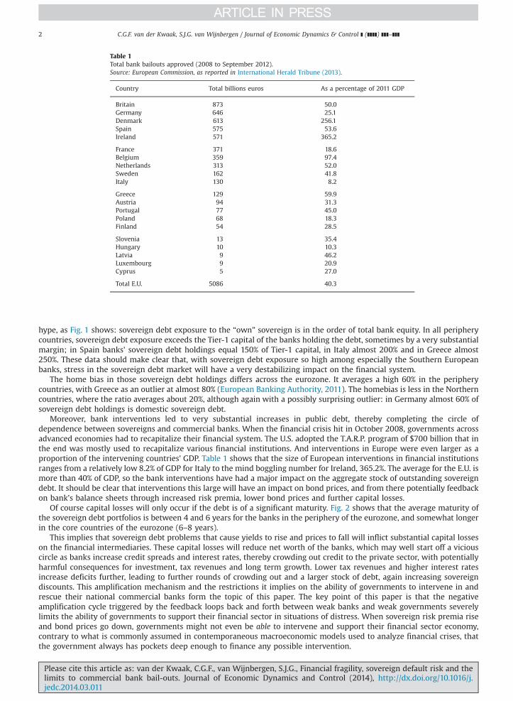
Table 1Total bank bailouts approved (2008 to September 2012).Source: European Commission, as reported in International Herald Tribune (2013).
Country Total billions euros As a percentage of 2011 GDP
Britain 873 50.0Germany 646 25.1Denmark 613 256.1Spain 575 53.6Ireland 571 365.2
France 371 18.6Belgium 359 97.4Netherlands 313 52.0Sweden 162 41.8Italy 130 8.2
Greece 129 59.9Austria 94 31.3Portugal 77 45.0Poland 68 18.3Finland 54 28.5
Slovenia 13 35.4Hungary 10 10.3Latvia 9 46.2Luxembourg 9 20.9Cyprus 5 27.0
Total E.U. 5086 40.3
C.G.F. van der Kwaak, S.J.G. van Wijnbergen / Journal of Economic Dynamics & Control ] (]]]]) ]]]–]]]2
hype, as Fig. 1 shows: sovereign debt exposure to the “own” sovereign is in the order of total bank equity. In all peripherycountries, sovereign debt exposure exceeds the Tier-1 capital of the banks holding the debt, sometimes by a very substantialmargin; in Spain banks' sovereign debt holdings equal 150% of Tier-1 capital, in Italy almost 200% and in Greece almost250%. These data should make clear that, with sovereign debt exposure so high among especially the Southern Europeanbanks, stress in the sovereign debt market will have a very destabilizing impact on the financial system.
The home bias in those sovereign debt holdings differs across the eurozone. It averages a high 60% in the peripherycountries, with Greece as an outlier at almost 80% (European Banking Authority, 2011). The homebias is less in the Northerncountries, where the ratio averages about 20%, although again with a possibly surprising outlier: in Germany almost 60% ofsovereign debt holdings is domestic sovereign debt.
Moreover, bank interventions led to very substantial increases in public debt, thereby completing the circle ofdependence between sovereigns and commercial banks. When the financial crisis hit in October 2008, governments acrossadvanced economies had to recapitalize their financial system. The U.S. adopted the T.A.R.P. program of $700 billion that inthe end was mostly used to recapitalize various financial institutions. And interventions in Europe were even larger as aproportion of the intervening countries' GDP. Table 1 shows that the size of European interventions in financial institutionsranges from a relatively low 8.2% of GDP for Italy to the mind boggling number for Ireland, 365.2%. The average for the E.U. ismore than 40% of GDP, so the bank interventions have had a major impact on the aggregate stock of outstanding sovereigndebt. It should be clear that interventions this large will have an impact on bond prices, and from there potentially feedbackon bank's balance sheets through increased risk premia, lower bond prices and further capital losses.
Of course capital losses will only occur if the debt is of a significant maturity. Fig. 2 shows that the average maturity ofthe sovereign debt portfolios is between 4 and 6 years for the banks in the periphery of the eurozone, and somewhat longerin the core countries of the eurozone (6–8 years).
This implies that sovereign debt problems that cause yields to rise and prices to fall will inflict substantial capital losseson the financial intermediaries. These capital losses will reduce net worth of the banks, which may well start off a viciouscircle as banks increase credit spreads and interest rates, thereby crowding out credit to the private sector, with potentiallyharmful consequences for investment, tax revenues and long term growth. Lower tax revenues and higher interest ratesincrease deficits further, leading to further rounds of crowding out and a larger stock of debt, again increasing sovereigndiscounts. This amplification mechanism and the restrictions it implies on the ability of governments to intervene in andrescue their national commercial banks form the topic of this paper. The key point of this paper is that the negativeamplification cycle triggered by the feedback loops back and forth between weak banks and weak governments severelylimits the ability of governments to support their financial sector in situations of distress. When sovereign risk premia riseand bond prices go down, governments might not even be able to intervene and support their financial sector economy,contrary to what is commonly assumed in contemporaneous macroeconomic models used to analyze financial crises, thatthe government always has pockets deep enough to finance any possible intervention.
Please cite this article as: van der Kwaak, C.G.F., van Wijnbergen, S.J.G., Financial fragility, sovereign default risk and thelimits to commercial bank bail-outs. Journal of Economic Dynamics and Control (2014), http://dx.doi.org/10.1016/j.jedc.2014.03.011i

Fig. 1. Sovereign debt exposure of banks to the domestic sovereign in the eurozone as a percentage of their total tier 1 capital. Core: AT: Austria,BE: Belgium, DE: Germany, FI: Finland, FR: France, NL: Netherlands. Periphery: ES: Spain, GR: Greece, IE: Ireland, IT: Italy, PT: Portugal.Source: European Banking Authority (2011), own calculations.
Fig. 2. Average maturity of the domestic sovereign debt exposure of the banking sector. Core: AT: Austria, BE: Belgium, DE: Germany, FI: Finland,FR: France, NL: Netherlands. Periphery: ES: Spain, GR: Greece, IE: Ireland, IT: Italy, PT: Portugal.Source: European Banking Authority (2011), own calculations.
Please cite this article as: van der Kwaak, C.G.F., van Wijnbergen, S.J.G., Financial fragility, sovereign default risk and thelimits to commercial bank bail-outs. Journal of Economic Dynamics and Control (2014), http://dx.doi.org/10.1016/j.jedc.2014.03.011i
C.G.F. van der Kwaak, S.J.G. van Wijnbergen / Journal of Economic Dynamics & Control ] (]]]]) ]]]–]]] 3

C.G.F. van der Kwaak, S.J.G. van Wijnbergen / Journal of Economic Dynamics & Control ] (]]]]) ]]]–]]]4
That this concern is not just a theoretical artifact was clearly shown in the case of Spain. Before the financial crisis started,the Spanish economy experienced a housing boom. When the bubble burst, Spanish banks were left with big losses on theirreal estate portfolios, effectively wiping out their net worth. This, in turn, depressed the flow of credit to the private sector,and contributed to the ensuing recession. At the same time government deficits soared, and within a couple of years Spanishdebt rose from 35% of GDP to more than 80% of GDP (Spanish Ministry of Economic Affairs, 2012). The Spanish governmentdecided to restructure the Spanish financial system in May 2012, and committed to debt-financed public recapitalizations incase banks would not be able to raise new capital privately. It was expected that the new flow of credit by a recapitalizedbanking system would restart the economy, and thereby improve the long term budget position of the Spanish government,which should be reflected in lower yields on current Spanish government bonds. Instead, yields soared, undermining anyeffect of the intended bank recapitalization, and the Spanish government had to apply for external funds from the ESM to betransmitted directly to the banks on June 25, 2012. Similar problems have emerged across Southern Europe, extremely so inIreland. There bank intervention was in fact the only source of the subsequent debt problems, prior to the recent crisis Irishdebt was as low as 25% of GDP (Eurostat, 2014) while their government budget was in fact in surplus in 2007. The bankrescue in 2008 led to an explosion of domestic debt, a collapse in debt prices and an effective drying up of capital marketaccess for Ireland.
In order to capture the above-described dynamics, we build a dynamic stochastic general equilibrium model thatincorporates balance sheet constrained financial intermediaries supplying loans both to firms and to the government (i.e.they hold sovereign debt on their balance sheet). We also explicitly introduce sovereign risk. The methodological innovationis the fact that we combine financial intermediaries in our macromodel that are balance sheet constrained while holdingboth corporate loans and government bonds subject to sovereign default risk. Through this channel we capture theinterconnectedness between the financial system and the fiscal problems of the government.
We introduce long term government bonds in a way similar to Woodford (1998, 2001), through a variable maturitystructure of government debt captured by the parameter ρ, through which we can obtain any duration between 1 periodbonds ðρ¼ 0Þ and perpetuals, or ‘consols’ ðρ¼ 1Þ.1 Introducing maturity structure allows us to capture the stylized facts fromFig. 2. Introducing maturities longer than the one period bonds commonly used in macroeconomic models is importantbecause of the link with capital losses for the already balance sheet constrained commercial banks in the model. The longerthe maturity of the government bonds, the higher the capital losses for the financial intermediaries, and the morepronounced the adverse effects on the economy in case of a financial crisis.
Long term government debt is commonly thought of as stabilizing because of lower roll over risk; while that isdoubtlessly true, we show that there is another side to this whereby long term debt may in fact exacerbate a given financialcrisis. We do not try to derive an optimal maturity structure balancing these two conflicting effects on financial fragility;instead, more modestly, we take the maturity structure as given, and show how lengthening the maturity structurestrengthens a poisonous link between financial fragility and sovereign weakness in the debt market.
Sovereign default risk is captured by postulating a so-called maximum level of (lump-sum) taxation that is politicallyfeasible, which is imposed by assumption. We then map this maximum level of taxation into a maximum level of debt. Weassume that the government follows a core tax policy that guarantees intertemporal solvency in the no default setup andcompute the amount of new debt that needs to be issued in order to finance all government obligations, and compare thiswith the maximum level of debt that is still politically feasible. If the so-called level of no default debt is smaller than themaximum level of debt, the government honors its obligations and does not default; when the no-default level exceeds themaximum level, a (partial) default occurs bringing back the number of government bonds to the maximum numberpossible.
We first use the model to assess the effect of varying the maturity of the government bonds on the impact of a financialcrisis. We then proceed to investigate the effect of a recapitalization of the financial sector that is announced at the onset ofa financial crisis, but implemented 4 quarters later, reflecting realistic delays in implementing rescue programs. This willintroduce anticipation effects coming in before the recapitalization itself due to the forward looking nature of the model. Wefinally introduce sovereign default risk, and compare the same recapitalization exercise but now in the presence ofendogenous sovereign default risk. In particular, we want to investigate whether and how financial sector bailout programsaffect sovereign default risk, and whether sovereign default risk can feedback to the financial sector, thereby underminingthe rescue action and creating an amplification mechanism exacerbating the initial impact of a financial shock.
Since the start of the credit crisis, the theoretical literature with general equilibrium models containing financial frictionsis growing, although Bernanke et al. (1999) preceded the crisis. Gertler and Karadi (2011) introduce financial intermediariesthat are balance sheet constrained by an agency problem between the deposit holders and the bank owners. This gives riseto an endogeneous leverage constraint, which becomes more binding when net worth is reduced by for example a negativeshock to the quality of the loans. Several others have a similar mechanism, for example Kiyotaki and Moore (1997), Gertlerand Kiyotaki (2010), and Kirchner and van Wijnbergen (2012), who include financial intermediaries holding short termgovernment debt besides loans to the private sector. The current paper extends that model by introducing long termgovernment bonds and sovereign default risk. Woodford (1998, 2001) introduces long term government debt by assumingthat the government is financed through a bond with infinite maturity. The stream of payments that the holder receives,
1 We are indebted to a referee for suggesting this approach.
Please cite this article as: van der Kwaak, C.G.F., van Wijnbergen, S.J.G., Financial fragility, sovereign default risk and thelimits to commercial bank bail-outs. Journal of Economic Dynamics and Control (2014), http://dx.doi.org/10.1016/j.jedc.2014.03.011i

C.G.F. van der Kwaak, S.J.G. van Wijnbergen / Journal of Economic Dynamics & Control ] (]]]]) ]]]–]]] 5
though, decreases each period by a factor ρr1, thereby creating a bond with an effective duration that depends on thefactor ρ. We follow this approach to modeling maturity. Gertler and Karadi (2013) also extend the number of assets held byfinancial intermediaries by letting them hold a long term government bond in the form of a perpetuity, a case that isencompassed as a special case in the setup used in this paper (for ρ¼ 1). The introduction of government bonds financed byfinancial intermediaries creates a second amplification mechanism, whereby increased government bond issuance, in orderto stimulate the economy, can crowd out financing of the private sector. These papers, however, do not take into account thepossibility of a government default. Acharya et al. (2011) have a setup containing both financial sector bailouts and sovereigndefault risk, but their analysis occurs within a partial equilibrium setup. Acharya and Steffen (2013), in their empiricalresearch on systemic risk of the European banking sector, find that European banks have been at the center of the two majorsystemic crises that have faced the financial system since 2007, and specifically that markets have demanded more capitalfrom banks with high sovereign debt exposures to peripheral countries, thereby indicating that sovereign debt holdingsfrom those countries are a major contributor to systemic risk.
Designing the optimal maturity structure of public debt is not the ambition of this paper (cf. Cole and Kehoe, 2000;Chatterjee and Eyigungor, 2012; Arellano and Ramanarayanan, 2012 for a discussion of the optimal maturity structure). Ourfocus is exclusively on the possibility of capital losses due to changes in sovereign risk. Sovereign default risk is captured inArellano (2008), which contains an endogeneous default mechanism somewhat similar in outcome to our approach (seeDavig et al., 2011 for a similar approach). Our setup is close to Schabert and van Wijnbergen (2011) who introduce sovereigndefault risk by assuming that there exists a (stochastic) maximum level of taxation that is politically feasible and derive fromthere a default risk discount that is increasing with government debt.
Section 2 describes the version of the model without sovereign default risk. Section 3 introduces sovereign default riskinto the model. Section 4 describes the calibration of the model. Section 5 discusses the results from the simulations, andSection 6 concludes.
2. Model description
Financial frictions are introduced in a manner similar to the approach pioneered by Gertler and Karadi (2011), but in oursetup banks extend credit to firms but also hold public sector debt on their balance sheet, like in Kirchner and vanWijnbergen (2012). Furthermore we introduce long term government debt and the possibility of a (partial) sovereigndefault. The government issues debt to financial intermediaries and raises taxes in a lump sum fashion from households tofinance its expenditures and meet debt service obligations of its existing debt. The default probability is increasing in thereal debt burden in a manner specified more fully below. The other part of the public sector is a central bank that is incharge of monetary policy. It sets the nominal interest rate on the deposits that the households bring to the financialintermediaries. The private sector consists of financial intermediaries and a non-financial sector that includes householdsand firms. The non-financial sector consists of capital producing firms that buy investment goods and used capital, andconvert these into capital that is sold to the intermediate goods producers. The intermediate goods producers use the capitalas an input, together with labor, to produce intermediate goods for the retail firms. Future gross profits are pledged to thefinancial intermediaries in order to obtain funding, hence the profits of the intermediate goods producers are zero inequilibrium. Each intermediate goods producer produces a differentiated product. The retail firms repackage and sell theretail products to the final goods producer. Every retail firm is a monopolist and charges a markup for his product. The finalgoods producers buy these goods and combine them into a single output good. The final good is purchased by thehouseholds for consumption, by the capital producers to convert it into capital, and by the government. The householdmaximizes life-time utility subject to a budget constraint, which contains income from deposits, profits from the firms, bothfinancial and non-financial, and from labor. The income is used for consumption, lump sum taxes and investments indeposits.
2.1. Household
The household sector consists of a continuum of infinitely lived households that exhibit identical preferences and assetendowments. A typical household consists of bankers and workers. Every period, a fraction f of the household members is abanker running a financial intermediary. A fraction 1� f of the household members is a worker. At the end of every period,all members of the household pool their resources, and every member of the household has the same consumption pattern.Hence there is perfect insurance within the household, and the representative agent representation is preserved. Everyperiod, the household earns income from the labor of the working members and the profits of the firms, which are ownedby the household. And deposits are paid back with interest. The household uses these funds to buy goods for consumptionor deposits them in financial intermediaries (but not the ones owned by the family, in order to prevent self-financing). Thehousehold members derive utility from consumption and leisure, with habit formation in consumption, in order to morerealistically capture consumption dynamics, as in Christiano et al. (2005). Households maximize expected discounted utility
maxfct þ s ;htþ s ;dtþ sg1s ¼ 0
Et ∑1
s ¼ 0βs log ctþ s�υct�1þ sð Þ�Ψh
1þφtþ s
1þφ
!" #;
Please cite this article as: van der Kwaak, C.G.F., van Wijnbergen, S.J.G., Financial fragility, sovereign default risk and thelimits to commercial bank bail-outs. Journal of Economic Dynamics and Control (2014), http://dx.doi.org/10.1016/j.jedc.2014.03.011i

C.G.F. van der Kwaak, S.J.G. van Wijnbergen / Journal of Economic Dynamics & Control ] (]]]]) ]]]–]]]6
βAð0;1Þ; υA ½0;1Þ; φZ0;
where ct is the consumption per household, and ht are the hours worked, subject to the following budget constraint:
ctþdtþτt ¼wthtþ 1þrdt� �
dt�1þΠt :
The household optimizes with respect to the budget constraint. Intermediary deposits dt�1 are deposited at t�1; they receiveinterest rt
dand repayment of principal at time t. wt is the real wage rate, τt are the lump sum tax payments the household has
to pay to the government, and Πt are the profits from the firms that are owned by the households. The profits of the financialintermediary are net of the startup capital for new bankers, as will be explained below. The first order conditions are nowgiven by
ct : λt ¼ ðct�υct�1Þ�1�υβEt ½ðctþ1�υctÞ�1�; ð1Þ
ht :Ψhφt ¼ λtwt ; ð2Þ
dt :1¼ βEt ½Λt;tþ1ð1þrdtþ1Þ�; ð3Þwhere λt is the Lagrange multiplier of the budget constraint, and Λt;tþ i ¼ λtþ i=λt is the stochastic discount factor for iZ0.
2.2. Financial intermediaries
Financial intermediaries lend funds obtained from households to intermediate goods producers and the government. Thebanker's balance sheet is given by
pj;t ¼ nj;tþdj;t ;
where pj;t are the assets of bank j in period t, nj;t and dj;t denote the net worth and deposits of bank j, respectively. Thefinancial intermediary invests its funds in claims issued by the intermediate goods producer, and in government bonds.Hence the asset side of the bank's balance sheet has the following structure:
pj;t ¼ qkt skj;tþqbt s
bj;t ;
where skj;t are the number of claims on the intermediate goods producers with price qtk, and sbj;t the number of government
bonds acquired by intermediary j, at a price qtb. The claims on the producers pay a net real return rktþ1 at the beginning of
period tþ1. Government bonds pay a net real return rbtþ1 at the beginning of period tþ1. Financial intermediaries earnthose returns on their assets, and pay a return on the deposits. The difference between the two is equal to the increase in thenet worth from one period to the next. The balance sheet of intermediary j then evolves as follows:
nj;tþ1 ¼ 1þrktþ1
� �qkt s
kj;tþ 1þrbtþ1
� �qbt s
bj;t� 1þrdtþ1
� �dj;tþng
j;tþ1� ~ngj;tþ1
¼ rktþ1�rdtþ1
� �qkt s
kj;tþ rbtþ1�rdtþ1
� �qbt s
bj;tþ 1þrdtþ1
� �nj;t
þτntþ1nj;t� ~τntþ1nj;t ;
where ngj;tþ1 ¼ τntþ1nj;t denotes the net worth provided by the government to the financial intermediary j (for example a
capital injection). ~ngj;tþ1 ¼ ~τntþ1nj;t denotes the repayment of government support received in previous periods.
The financial intermediary maximizes expected profits. The probability that the banker has to exit the industry nextperiod equals 1�θ, in which case he will bring his net worth nj;tþ1 to the household. So θ is the probability that he will beallowed to continue operating. The banker discounts these outcomes by the stochastic discount factor βΛt;tþ1, since financialintermediaries are owned by households. The banker's objective is then given by the following recursively definedmaximand:
Vj;t ¼max Et ½βΛt;tþ1fð1�θÞnj;tþ1þθVj;tþ1g�;where Λt;tþ1 ¼ λtþ1=λt . We conjecture the solution to be of the following form, and later check whether this is the case:
Vj;t ¼ νkt qkt skj;tþνbt qbt sbj;tþηtnj;t : ð4Þ
Like in Gertler and Karadi (2011), bankers can divert a fraction λ of the assets at the beginning of the period, and transferthese assets costlessly back to the household. If that happens, the depositors will force the intermediary into bankruptcy, butwill only be able to recover the remaining fraction 1�λ of the assets of the financial intermediary. Hence lenders will onlysupply funds if the gains from stealing are lower than the continuation value of the financial intermediary. This gives rise tothe following constraint:
Vj;tZλ qkt skj;tþqbt s
bj;t
� �) νkt q
kt s
kj;tþνbt qbt sbj;tþηtnj;tZλ qkt s
kj;tþqbt s
bj;t
� �: ð5Þ
Please cite this article as: van der Kwaak, C.G.F., van Wijnbergen, S.J.G., Financial fragility, sovereign default risk and thelimits to commercial bank bail-outs. Journal of Economic Dynamics and Control (2014), http://dx.doi.org/10.1016/j.jedc.2014.03.011i

C.G.F. van der Kwaak, S.J.G. van Wijnbergen / Journal of Economic Dynamics & Control ] (]]]]) ]]]–]]] 7
The optimization problem can now be formulated in the following way:
maxfqkt skj;t ;qbt sbj;t g
Vj;t ; s:t: Vj;tZλ qkt skj;tþqbt s
bj;t
� �:
From the first order conditions we find that νbt ¼ νkt . Hence the leverage constraint (5) can be rewritten in the following way:
νkt qkt skj;tþqbt s
bj;t
� �þηtnj;tZλ qkt s
kj;tþqbt s
bj;t
� �) qkt s
kj;tþqbt s
bj;trϕtnj;t ;
ϕt ¼ηt
λ�νkt; ð6Þ
where ϕt denotes the ratio of assets to net worth, which can be seen as the leverage constraint of the financial intermediary.The intuition for the leverage constraint is straightforward: a higher shadow value of assets νt
kimplies a higher value from
an additional unit of assets, which raises the continuation value of the financial intermediary, thereby making it less likelythat the banker will steal. A higher shadow value of net worth ηt implies a higher expected profit from an additional unit ofnet worth, while a higher fraction λ implies that the banker can steal a larger fraction of assets, which induces the householdto provide less funds to the banker, resulting in a lower leverage ratio everything else equal. Substitution of the conjecturedsolution into the right hand side of the Bellman equation gives the following expression for the continuation value of thefinancial intermediary:
Vj;t ¼ Et ½Ωtþ1nj;tþ1�;Ωtþ1 ¼ βΛt;tþ1fð1�θÞþθ½ηtþ1þνktþ1ϕtþ1�g:
Ωtþ1 can be thought of as a stochastic discount factor that incorporates the financial friction. Now substitute the expressionfor next period's net worth into the expression above:
Vj;t ¼ Et ½Ωtþ1nj;tþ1�
¼ Et Ωtþ1 1þrktþ1
� �qkt s
kj;tþ 1þrbtþ1
� �qbt s
bj;t� 1þrdtþ1
� �dj;tþng
j;tþ1� ~ng
j;tþ1
� �� �
¼ Et Ωtþ1 rktþ1�rdtþ1
� �qkt s
kj;tþ rbtþ1�rdtþ1
� �qbt s
bj;tþ 1þrdtþ1þτntþ1� ~τ
n
tþ1
� �nj;t
n oh i: ð7Þ
After combining the conjectured solution with (4), we find the following first order conditions:
ηt ¼ Et Ωtþ1 1þrdtþ1þτntþ1� ~τn
tþ1
� �h i; ð8Þ
νkt ¼ Et Ωtþ1 rktþ1�rdtþ1
� �h i; ð9Þ
νbt ¼ νkt ¼ Et Ωtþ1 rbtþ1�rdtþ1
� �h i; ð10Þ
Ωtþ1 ¼ βΛt;tþ1 1�θð Þþθ ηtþ1þνktþ1ϕtþ1
h in o:
2.2.1. Financial sector supportWe assume that support provided to an individual intermediary, if provided, will be proportional to the intermediary's
net worth in the previous period. Hence individual financial support is given by
ngj;t ¼ τnt nj;t�1; ζr0; lZ0;
τnt ¼ ζðξt� l�ξÞ:Repayment of the support is parametrized proportional to the sector's net worth in the period preceding the pay backperiod:
~ngj;t ¼ ~τnt nj;t�1;
where ~τnt is a scaling factor that is obviously time dependent and incorporates the return paid by the sector to thegovernment over the support funds.
2.2.2. Aggregation of financial variablesIntegrating the individual balance sheets of the financial intermediaries yields the aggregate balance sheet of the
financial sector:
pt ¼ ntþdt : ð11ÞAggregation over the asset side of the balance sheet gives the composition of the aggregated financial system:
pt ¼ qkt skt þqbt s
bt : ð12Þ
Please cite this article as: van der Kwaak, C.G.F., van Wijnbergen, S.J.G., Financial fragility, sovereign default risk and thelimits to commercial bank bail-outs. Journal of Economic Dynamics and Control (2014), http://dx.doi.org/10.1016/j.jedc.2014.03.011i

C.G.F. van der Kwaak, S.J.G. van Wijnbergen / Journal of Economic Dynamics & Control ] (]]]]) ]]]–]]]8
ϕt does not depend on firm specific factors, so we can aggregate the leverage constraint (6) across financial intermediaries tolink sector wide assets and net worth:
pt ¼ qkt skt þqbt s
bt ¼ ϕtnt : ð13Þ
The share of assets invested in private loans is given by
ωt ¼ qkt skt =pt : ð14Þ
At the end of the period, only a fraction θ of the current bankers will remain a banker, while the remaining fraction 1�θ willbecome a worker. Bankers only pay out dividends at the moment they quit the banking business. If they do not quit, theyretain their net worth and carry it into the next period. So the aggregate net worth of the continuing bankers at the end ofthe period equals:
ne;t ¼ θ rkt �rdt Þqkt�1skt�1þ rbt �rdt
� �qbt�1s
bt�1þ 1þrdt
� �nt�1
� i:
hExiting bankers bring their net worth into the household's income. A fraction 1�θ of the f bankers leave the financialindustry each period, equal to a fraction ð1�θÞf of the household. The same fraction of the household will enter the financialindustry next period. We assume that the household will provide a starting net worth to the new bankers proportional tothe assets of the old bankers, equal to a fraction χ=ð1�θÞ of the assets of the old bankers, as in Gertler Karadi (2011). Hencethe aggregate net worth of the new bankers will be equal to:
nn;t ¼ χpt�1:
Then the total net worth at the end of the period, after the lottery has decided which bankers will leave the industry, is
nt ¼ ne;tþnn;tþngt � ~ng
t
¼ θ rkt �rdt� �
qkt�1skt�1þ rbt �rdt
� �qbt�1s
bt�1þ 1þrdt
� �nt�1
h iþχpt�1þng
t � ~ngt ; ð15Þ
where ntgand ~ng
t are aggregate financial sector support and payback of (earlier) financial support, respectively. Sinceindividual support is proportional to the individual intermediary's net worth, it is straightforward to get aggregate financialsector support:
ngt ¼ ζðξt� l�ξÞnt�1: ð16Þ
Similarly, we can aggregate financial sector payback:
~ngt ¼ ~τnt nt�1 ) ~τnt ¼ ~ng
t =nt�1: ð17ÞWe derive the expression for ~ng
t below, in Section 2.4.
2.3. Production side
The production side of the economy is modeled in now standard New-Keynesian fashion. We have a continuum ofintermediate goods producers indexed by iA ½0;1� borrowing from the financial intermediary to purchase the capitalnecessary for production. With the proceeds from the sale of the output and the sale of the capital after it has been used, thefirms pay workers and pay back the loans to the financial intermediary. The capital producers buy the capital that has beenused, and transform the used capital, together with the goods purchased from the final goods producers, into new capital.This new capital is sold to the intermediate goods producers, who will use it for production next period. A continuum ofretail firms, indexed by f A ½0;1�, repackage the products bought from the intermediate goods producers to produce a uniquedifferentiated retail product. The retail firms sell their products to a continuum of final goods producers. The products aredifferentiated, so each individual retail firm has “local” monopoly power, and charges a markup. A randomly selectedfraction ψ of all retail firms cannot change prices in a given period. The final goods producers convert the inputs from theretail firms into final goods. Due to perfect competition, profits are zero in equilibrium, and the final goods are sold to thehouseholds, the government, and the capital producers. We only derive the non-standard parts, and refer to Appendix A.2for the rest of the production process.
2.3.1. Capital producersAt the end of period t, when the intermediate goods firms have produced, the capital producers buy the remaining stock
of capital ð1�δÞξtkt�1 from the intermediate goods producers at a price qtk. They combine this capital with goods bought
from the final goods producers (investment it) to produce next period's beginning of period capital stock kt. This capital isbeing sold to the intermediate goods producers at a price qt
k. We assume that the capital producers face convex adjustment
costs when transforming the final goods bought into capital goods, set up such that changing the level of gross investment iscostly. Hence we get
kt ¼ 1�δð Þξtkt�1þ 1�Ψ ιtð Þð Þit ; Ψ xð Þ ¼ γ
2ðx�1Þ2; ιt ¼ it=it�1: ð18Þ
Please cite this article as: van der Kwaak, C.G.F., van Wijnbergen, S.J.G., Financial fragility, sovereign default risk and thelimits to commercial bank bail-outs. Journal of Economic Dynamics and Control (2014), http://dx.doi.org/10.1016/j.jedc.2014.03.011i

C.G.F. van der Kwaak, S.J.G. van Wijnbergen / Journal of Economic Dynamics & Control ] (]]]]) ]]]–]]] 9
ξt represents a capital quality shock which will be discussed later. Profits are passed on to the households, who own thecapital producers. The profit at the end of period t equals
Πct ¼ qkt kt�qkt ð1�δÞξtkt�1� it :
The capital producers maximize expected current and (discounted) future profits (where we substitute in (18)):
maxfit þ ig1i ¼ 0
Et ∑1
i ¼ 0βiΛt;tþ iðqktþ ið1�Ψ ðιtþ iÞÞitþ i� itþ iÞ
" #:
Differentiation with respect to investment gives the first order condition for the capital producers
qkt ð1�Ψ ðιtÞÞ�1�qkt ιtΨ0ðιtÞþβEtΛt;tþ1qktþ1ι
2tþ1Ψ
0ðιtþ1Þ ¼ 0;
which gives the following expression for the price of capital:
1qkt
¼ 1� γ2
itit�1
�1� 2
� γitit�1
itit�1
�1�
þβEt Λt;tþ1qktþ1
qkt
itþ1
it
� 2
γitþ1
it�1
� " #: ð19Þ
2.3.2. Intermediate goods producersThere exists a continuum of intermediate goods producers indexed by iA ½0;1�. Each of these firms produces a
differentiated good. The intermediate goods producers obtain funds from the financial intermediaries by pledging nextperiod's profits, so banks are exposed to downside risk. We assume that there are no financial frictions between the financialintermediaries and the intermediate goods producers. The securities issued by the intermediate goods producers are bestconsidered as state-contingent debt, like in Gertler and Kiyotaki (2010).2 The price of the claims is equal to qkt�1, and pays astate-contingent net real return rt
kin period t. The production technology of the intermediate goods producers is given by
yi;t ¼ atðξtki;t�1Þαh1�αi;t ;
logðatÞ ¼ ρa logðat�1Þþεa;t ; logðξtÞ ¼ ρξ logðξt�1Þþεξ;t :Both (log of) total factor productivity at and capital quality ξt are AR(1) processes driven by random shocks εa;t �Nð0; s2aÞ andεξ;t �Nð0;s2ξ Þ. The intermediate goods producer acquires the capital at the end of period t�1 and uses it for production inperiod t. The capital quality shock ξt occurs at the beginning of period t, so ξtki;t�1 is the effective stock of capital used forproduction in period t. A negative realization of εξ;t lowers the quality of the capital stock, hence the return on the claims of thefinancial intermediary will be lower. The intermediate goods producer hires labor hi;t for a wage rate wt after the shock ξthas been realized. When the firm has produced in period t, the output is sold for price mt to the retail firms. mt is the relativeprice of the intermediate goods with respect to the price level of the final goods, i.e. mt ¼ Pm
t =Pt . A fraction δ of the capitalstock ξtki;t�1 is used up in the production process. The intermediate goods producing firms sell back what is left of theeffective capital stock to the capital producers for the end-of-period price of qt
kand thus receives qkt ð1�δÞξtki;t�1. Hence period
t profits are
Πi;t ¼mtatðξtki;t�1Þαh1�αi;t þqkt ð1�δÞξtki;t�1�ð1þrkt Þqkt�1ki;t�1�wthi;t :
The intermediate goods producing firms maximize expected current and future profits using the household's stochasticdiscount factor βsΛt;tþ s (since they are owned by the households), taking all prices as given
maxfkt þ s ;ht þ sg1s ¼ 0
Et ∑1
s ¼ 0βsΛt;tþ sΠi;tþ s
� �:
The resulting first order conditions are derived in a straightforward manner, and can be found in the appendix.
2.4. Government
The government issues bt bonds in period t, and raises qbt bt with qtbbeing the market price of bonds. We parametrize the
maturity structure of government debt like Woodford (1998, 2001): maturity is introduced by assuming that onegovernment bond issued in period t pays out rc units (in real terms) in period tþ1, ρrc real units in period tþ2, ρ2rc realunits in period tþ3, etc. This is equivalent to a payout of rc plus ρ times one newly issued bond in period tþ1, with a valueof rcþρqbtþ1. So ρ pins down the maturity of government debt, and government debt service in period t is ðrcþρqbt Þbt�1.The duration3 of public debt is 1=ð1�βρÞ. The government also raises revenue by levying lump sum taxes on the households.Government purchases are constant: gt ¼ G. Furthermore the government may provide assistance to the financial
2 It is therefore better to think of the claims of financial intermediaries as equity. Occhino and Pescatori (2010) explicitly model loans to producers witha fixed face value, where the goods producers have the possibility of defaulting on the loans. We refrain from explicitly modelling this default possibility,and note the equity characteristics of debt in the real world when firms are short of funds to pay off the loans.
3 Duration is defined as ∑1j ¼ 1jβ
jðρj�1rcÞ=∑1j ¼ 1β
jðρj�1rcÞ
Please cite this article as: van der Kwaak, C.G.F., van Wijnbergen, S.J.G., Financial fragility, sovereign default risk and thelimits to commercial bank bail-outs. Journal of Economic Dynamics and Control (2014), http://dx.doi.org/10.1016/j.jedc.2014.03.011i

C.G.F. van der Kwaak, S.J.G. van Wijnbergen / Journal of Economic Dynamics & Control ] (]]]]) ]]]–]]]10
intermediaries by injecting capital ntg, and it receives repayment of support administered previously ( ~ng
t ). So the budgetconstraint becomes
qbt btþτtþ ~ngt ¼ gtþng
t þ rcþρqbt� �
bt�1 ¼ gtþngt þ
rcþρqbtqbt�1
!qbt�1bt�1;
⟹qbt btþτtþ ~ngt ¼ gtþng
t þð1þrbt Þqbt�1bt�1: ð20Þ
rtbis the real return on government bonds:
1þrbt ¼rcþρqbtqbt�1
: ð21Þ
The tax rule of the government is given by a rule which Bohn (1998) has shown secures sustainability:τt ¼ τþκbðbt�1�bÞþκnng
t ; κbA ð0;1�; κnA ½0;1�: ð22Þ
b is the steady state level of debt. κn controls the way government transfers to the financial sector are financed. If κn ¼ 0,support is financed by new debt. κn ¼ 1 implies that the additional spending is completely financed by increasing lump sumtaxes. We parametrize government support as follows:
ngt ¼ τnt nt�1; ζr0; lZ0;
τnt ¼ ζðξt� l�ξÞ: ð23Þ
Thus the government provides funds to the financial sector if ζo0 (a negative shock to the quality of capital). Depending onthe value of l, the government can provide support instantaneously (l¼0), or with a lag (l40). Furthermore, ϑ indicates theextent to which the government needs to be repaid:
~ngt ¼ ϑng
t� e; ϑZ0; eZ1: ð24Þ
ϑ¼ 0 means that the support is a gift from the government. In case ϑ¼ 1, the government aid is a zero interest loan, while aϑ41 implies that the financial intermediaries have to pay interest over the support received earlier.4 The parameter edenotes the amount of time after which the government aid has to be paid back.
2.5. Central Bank
The Central Bank sets the nominal interest rate on deposits rtnaccording to a standard Taylor rule, in order to minimize
output and inflation deviations:
rnt ¼ ð1�ρrÞðrnþκπðπt�π Þþκy logðyt=yt�1ÞÞþρrrnt�1þεr;t ; ð25Þ
where εr;t �Nð0; s2r Þ, and κπ40 and κy40. The parameter π is the target inflation rate. We choose κπ41; κy40 (leaningagainst the wind). The real interest rate on deposits then equals:
1þrdt ¼ ð1þrnt�1Þ=πt : ð26Þ
2.6. Market clearing
Equilibrium requires that the number of claims owned by the financial intermediaries (stk) must be equal to aggregate
capital (kt), while the number of government bonds owned by the financial sector (stb) must be equal to the number of bonds
issued by the government (bt):
skt ¼ kt ; ð27Þ
sbt ¼ bt : ð28Þ
Goods market clearing requires that the aggregate demand equals aggregate supply:
ctþ itþgt ¼ yt : ð29Þ
4 The case where ϑ41 happened in the Netherlands, where financial intermediaries received government aid with a penalty rate of 50%.
Please cite this article as: van der Kwaak, C.G.F., van Wijnbergen, S.J.G., Financial fragility, sovereign default risk and thelimits to commercial bank bail-outs. Journal of Economic Dynamics and Control (2014), http://dx.doi.org/10.1016/j.jedc.2014.03.011i

C.G.F. van der Kwaak, S.J.G. van Wijnbergen / Journal of Economic Dynamics & Control ] (]]]]) ]]]–]]] 11
3. Extension with government default
3.1. The default process
The government follows a simple tax rule consistent with the long term sustainability requirements outlined in Bohn(1998):
τtþ1 ¼ τþκbðbt�bÞþκnngtþ1:
But we furthermore assume that there is a maximum level beyond which taxes are not politically sustainable anymore, likein Schabert and van Wijnbergen (2011), or like the ‘fiscal limit’ in Davig et al. (2011). This fiscal limit is not derivedendogeneously, but is instead introduced by assumption. This fiscal limit translates in a maximum level of debt that canbe sustained, and introduces the possibility of (partial) default if shocks trigger higher levels of debt than the maximumlevel of debt implied by the ‘fiscal limit’. Such a maximum level of taxes should probably be stochastic, as in Schabert andvan Wijnbergen (2011), but for simplicity and without much loss of generality we follow Davig et al. (2011) in assuming it tobe fixed and known to be equal to τmax. The maximum level of debt bt
maximplied by this fiscal limit then becomes
bmaxt ¼ bþτ
max�τκb
: ð30Þ
As shown in Section 2.4, the Woodford (1998, 2001) maturity structure leads to a government liability before financing ofthe primary deficit equal to Lt
q¼ðrcþρqbt Þbt�1. Thus in the absence of government default, the end of period debt wouldbecome
qbt~bt ¼ Lqt þgtþng
t �τt� ~ngt ;
where ~bt denotes the level of government debt if the government would not default on its obligations. The constraint can berewritten in the following way:
qbt~btþτtþ ~ng
t ¼ gtþngt þðrcþρqbt Þbt�1: ð31Þ
As long as the level of debt that the government needs to issue in order not to default ( ~bt) is smaller than the maximumlevel of debt bt
max, the actual government debt bt will be equal to the no default level of government debt ~bt . But when
~bt4bmaxt , we assume that the government defaults on a large enough fraction of its outstanding debt and debtservice
obligations to bring the actual end-of-period debt down to btmax
:
bt ¼~bt if ~btrbmax
t ;
bmaxt if ~bt4bmax
t :
8<: ð32Þ
We assume that the government achieves this outcome through orderly renegotiation with its creditors. Since creditorshave rational expectations, they know that they will not be able to get more from the government than what thegovernment can raise through the maximum level of taxes τmax. The debt/tax limit may nevertheless become bindingbecause of random shocks to the system affecting debt both directly and through the government's tax and expenditurerules. We abstain from free-rider problems among creditors and assume that all creditors participate in the renegotiation.The government partially reneges on its debtservice obligations, applying the same discount Δt as used in the debtrestructuring.5 We can see the debt structure bt as the blue solid line in Fig. A1 (see appendix). It is informative to write thedebt level structure (32) in the following way:
bt ¼minð ~bt ; bmaxt Þ ¼ bmax
t �maxðbmaxt � ~bt ;0Þ: ð33Þ
The second term is like the payout of a put option at maturity with underlying process ~bt and strike price btmax
; see Claessensand van Wijnbergen (1993) who apply such a model in their evaluation of the Mexican Brady plan debt restructuring usingoption pricing methodology for ex ante valuation. As an ex post default function, however, (33) is not differentiable atbt ¼ bmax
t which creates severe problems in solving the model. We therefore approximate the ex post default rule by itsex ante option pricing based valuation formula.6 Since option prices close to maturity are a good approximation to option-payouts at maturity, our option based formula approximates (33) closely but without differentiability problems. This isdescribed in detail in Appendix A.3.
5 For analytical simplicity and without loss of generality we choose an equal discount percentage for both current debtservice and the existing stockof debt.
6 We acknowledge that we introduce an approximation error in this way. In our simulations, though, we never reach the maximum level of debt, andfind that the government maximally defaults over less than 1.5% of the outstanding debt stock. Hence the sovereign default risk operates mostly through anex ante anticipation effect. We therefore think that the approximation does not significantly affect our results, see also the Journal's Online SupplementaryArchive.
Please cite this article as: van der Kwaak, C.G.F., van Wijnbergen, S.J.G., Financial fragility, sovereign default risk and thelimits to commercial bank bail-outs. Journal of Economic Dynamics and Control (2014), http://dx.doi.org/10.1016/j.jedc.2014.03.011i

C.G.F. van der Kwaak, S.J.G. van Wijnbergen / Journal of Economic Dynamics & Control ] (]]]]) ]]]–]]]12
3.2. Default and the government budget constraint
Of course this default process has implications for the government budget constraint. When ~btrbmaxt , Δt ¼ 0 but when
~bt4bmaxt , the old government debt bt�1 is restructured by converting the old bonds into new bonds against a pro-rata
discount high enough to avoid overshooting the maximum debt level. Both coupon payments and all existing bonds arereduced by a factor ð1�ΔtÞ This implies that the government saves an amount equal to Δtðrcþρqbt Þbt�1 on new debtissuance. The flow budget constraint of the government in period t thus becomes
qbt bt ¼ Lqt þgtþngt �τt� ~ng
t �Δtðrcþρqbt Þbt�1;
with Δt ¼ 0 when there is no default. This can be rearranged to get
qbt btþτtþ ~ngt ¼ gtþng
t þð1�ΔtÞðrcþρqbt Þbt�1: ð34Þ
3.3. Financial intermediaries and default
The returns to the financial intermediaries holding the sovereign debt are of course affected. Call the default inclusivereturn rbnt , which is given by
1þrbnt ¼ 1�Δtð Þð1þrbt Þ ¼ 1�Δtð Þ rcþρqbtqbt�1
!: ð35Þ
This definition of the return on sovereign debt captures the complete direct impact of the possible default on financialintermediaries holding the debt, so we do not need to change anything after the introduction of possible sovereign defaults otherthan replacing rt
bby rbnt . This in turn implies that the expression for the leverage constraint remains unchanged, as well
as the expressions for the shadow value of private loans and net worth, and that the equations for the shadow value ofgovernment bonds and the law of motion of net worth of financial intermediaries only need minor adjustment (replacement ofrtbby rbnt ):
νbt ¼ Et Ωtþ1 rbntþ1�rdtþ1
� �h i; ð36Þ
nt ¼ θ rkt �rdt� �
qkt�1skt�1þ rbnt �rdt
� �qbt�1s
bt�1þ 1þrdt
� �nt�1
h iþχpt�1þng
t � ~ngt : ð37Þ
4. Calibration
4.1. No default version
We calibrate the model on a quarterly frequency. The parameter values can be found in Table 2. Most of the parametersare common in the literature on DSGE models, or frequently used in models containing financial frictions. We mostly followthe calibration of Gertler and Karadi (2011). This is the case for the subjective discount factor β, the degree of habit formationυ, the Frisch elasticity of labor supply.7 φ�1, the elasticity of substitution among intermediate goods ϵ, the price rigidityparameter ψ, the effective capital share α, and the investment adjustment cost parameter γ. The calibration of the financialvariables is also taken from Gertler and Karadi (2011). The steady state leverage ratio is set to 4, while the credit spread Γ isset to 100 basis points annually (which amounts to Γ ¼ 0:0025), which coincides with the pre-2007 spreads in US financialdata between BAA corporate and government bonds. The parameter θ is calibrated by taking the average survival period(Θ¼ 1=ð1�θÞ) to be equal to 36 quarters, or θ¼ 0:9722. The parameters in the Taylor rule are set to conventional values.
The feedback from government debt on taxes is set to a value such that both the model with and without default arestable. We calibrate the steady state ratios of investment and government spending over GDP, i=y and g=y to 20%(a reasonable value for OECD countries), by calibrating the depreciation parameter δ. The fixed payment in real terms thatthe holder of government bonds receives each period is set to 0.04. Different values have been tried but do not significantlyaffect the results. In our base case we set the maturity parameter at ρ¼ 0:96, equivalent to an average duration of 5 years.The steady state bond price, though, changes as we vary ρ in the first experiment, the parameter governing the averageduration of government debt. In order for different maturities to be comparable, we must make sure that the fraction ofgovernment debt on the balance sheet of the financial intermediaries does not change. Hence we calibrate on the
7 As a robustness check we have set φ¼ 4. The results carry over qualitatively, although labor supply becomes more persistent, and thereforemoderates the financial crisis. We have also investigated an RBC version of the model, and found that the effect from the maturity parameter ρ becomesless severe, while preserving the results qualitatively. See also the Journal's Online Supplementary Archive.
Please cite this article as: van der Kwaak, C.G.F., van Wijnbergen, S.J.G., Financial fragility, sovereign default risk and thelimits to commercial bank bail-outs. Journal of Economic Dynamics and Control (2014), http://dx.doi.org/10.1016/j.jedc.2014.03.011i

Table 2Model parameters.
Parameter Value Definition
Householdsβ 0.990 Discount rateυ 0.815 Degree of habit formationΨ 3.409 Relative utility weight of laborφ 0.276 Inverse Frisch elasticity of labor supply
Financial intermediariesλ 0.3863 Fraction of assets that can be divertedχ 0.0021 Proportional transfer to entering bankersθ 0.9722 Survival rate of the bankersΓ 0.0025 Steady state credit spread E½rk�rd�
Intermediate good firmsϵ 4.176 Elasticity of substitutionψ 0.779 Calvo probability of keeping prices fixedα 0.330 Effective capital share
Capital good firmsγ 1.728 Investment adjustment cost parameterδ 0.0494 Depreciation rate
Autoregressive componentsρz 0.95 Autoregressive component of productivityρξ 0.66 Autoregressive component of capital qualityρr 0 Interest rate smoothing parameter
Policyrc 0.04 Real payment to government bondholderρ 0.96 Parameter government debt duration (5 years)κb 0.050 Tax feedback parameter from government debtκπ 1.500 Inflation feedback on nominal interest rateκy 0.125 Output feedback on nominal interest rate
Default parametersΔ 0.005 Steady state share of default indicator
Shockssz 0.010 Standard deviation productivity shocksξ 0.050 Standard deviation capital quality shocksr 0.0025 Standard deviation interest rate surprise shock
Option parametersr �0.0273 Compounded risk-free interest rates 0.5031 Standard deviation underlying processT 0.1107 Time to maturity
C.G.F. van der Kwaak, S.J.G. van Wijnbergen / Journal of Economic Dynamics & Control ] (]]]]) ]]]–]]] 13
outstanding government liabilities as a fraction of GDP qbb=y instead of b=y, and set it equal to 2.4, implying an annualdebt-to-GDP ratio of 60%. Even though government financing by financial intermediaries accounts for only a small part inthe US, most financial friction models have been calibrated on US data. We follow the conventional calibration. The purposeof this paper is not to perform quantitative exercises specifically focused on the debt-distressed European peripheryeconomies; our aim is more generally to highlight the relevant mechanisms, leaving calibration on European data for thefuture. We perform robustness checks to make sure that the mechanism does not depend on a specific set of parameters. Weassume more aggressive monetary policy in the face of a credit crisis, and hence set ρr ¼ 0 in times of crisis. We think thiscaptures the way central banks reacted when the financial crisis erupted. A credit crisis is represented by a negative shock tocapital quality ξt of 5% on impact, with an autocorrelation coefficient ρξ ¼ 0:66, as in Gertler and Karadi (2011).
4.2. Default calibration
In this section we describe the calibration when sovereign default risk is introduced. The calibration of the real economyis not affected by the introduction of sovereign default risk. For the financial sector, the steady state bond price qb changes,and hence b. We calibrate the maximum level of government liabilities qbbmax=y to be at 90% of annual steady state GDP.Different values could have been chosen, but the main point of the paper is to show the mechanisms that interplay whendebt levels get close to the maximum level of debt. The steady state fraction of government liabilities qbb=y on the balancesheet of financial intermediaries does not change, since it is still calibrated to hit the 60% annual steady state output target.The reason for this freedom is the fact that we have a new variable, the level of debt in case of no government debt ~bt , andthe steady state tax rate that we can adjust in order to still be able to hit our original targets. The steady state default
Please cite this article as: van der Kwaak, C.G.F., van Wijnbergen, S.J.G., Financial fragility, sovereign default risk and thelimits to commercial bank bail-outs. Journal of Economic Dynamics and Control (2014), http://dx.doi.org/10.1016/j.jedc.2014.03.011i
C.G.F. van der Kwaak, S.J.G. van Wijnbergen / Journal of Economic Dynamics & Control ] (]]]]) ]]]–]]]14
probability is set at a rather conservative estimate of Δ ¼ 0:005, which implies an annual default probability of 2%, which issmall given the observed bond spreads in the European periphery.
There are two ways in which we calibrate the model, which are in detail described in the appendix. We apply calibrationstrategy 1 when far away from the debt limit. In this case we always apply Δ ¼ 0:005. When the steady state level ofgovernment debt comes close to the maximum level of debt, though, this strategy cannot be followed anymore, due tonumerical problems. This is the case for the last exercise, in which we investigate a delayed recapitalization when the steadystate government liabilities are at 80% of annual steady state GDP. First we find the parameters of the (option)approximation when qbb=y is at 75% of annual steady state GDP. Calibration strategy 1 cannot go further than this whenthe maximum level of government liabilities is at 90% of annual steady state GDP. We therefore change to calibrationstrategy 2 which can still be applied, and calibrate the model at 80% of annual steady state GDP. This changes the steadystate default probability to Δ ¼ 0:0068.
5. Results
As a prelude to the main results about the interaction between financial fragility, sovereign debt and commercial bankrescues, we first investigate the effect of a financial crisis, initiated through a credit (capital quality) shock in the model, toset the stage for the interventions that form the main topic of this paper. A special point of interest highlighted in thissubsection is the crucial importance of the maturity of sovereign debt. We then analyze the consequences of a classiccommercial bank recapitalization by the government, where we realistically assume that the recaps are implemented 4quarters after the announcement. Then we show that introducing sovereign default risk exacerbates the poisonouslynegative interactions between sovereign debt holdings of commercial banks and debt financed rescue attempts.
5.1. The macroeconomic impact of a financial crisis
As a prelude to the analysis of the interaction between sovereign debt and bank rescues, we first set the benchmark,a financial crisis without government intervention to support banks. Like Gertler and Karadi (2011), we model a financialcrisis as a decrease in the capital quality ξt. A deterioration of capital quality induces losses at the financial intermediaries onthe loans provided to the intermediate goods producers. As a consequence, the net worth of the financial intermediariesdecreases, and hence the intermediaries become more balance sheet constrained, and the credit spread increases by almost120 basis points in the short maturity case (which corresponds to an average maturity of 2 quarters). The lower quality ofcapital also decreases the expected productivity from the capital that is purchased with the loans, and because of the lowernet worth, the financial intermediaries have to cut back on lending, which further reduces the price of capital. Because ofclassic Dornbusch style overshooting, the price collapse leads to a higher expected return on the loans once the shock hashit. In response, financial intermediaries sell government bonds, thereby pushing down the current bond price, which inturn inflicts further capital losses on the financial intermediaries. This process continues until the forward looking expectedreturn on government bonds has increased sufficiently to make the intermediaries willingly hold the outstanding stock ofbonds. In the process, financial net worth falls further; the intermediaries' balance sheet further deteriorates, raisingborrowing costs and so on. What we see (in the plots collected in Fig. 3) is a pro-cyclical amplification cycle wherebyinvestment and eventually capital drop by more than 10%.
A third balance sheet effect that plays a role was highlighted by Kirchner and van Wijnbergen (2012) and is due tocrowding out by government debt. Government spending gt is fixed; then government borrowing is primarily affected bythe bond price qbt . Since the increase in the (expected) interest rates on private loans pushes up the (expected) interest rateson government debt, the bond price drops. Besides inflicting capital losses on the financial intermediaries, it also increasesthe number of bonds the government needs to issue for a given amount of expenditures. Issuing more bonds implies thatthere are more creditors to which the government has to pay the fixed payment rc, implying higher borrowing needs infuture periods. Hence a smaller proportion of the intermediaries' balance sheets is available for financing the capitalpurchases of the intermediate goods producers. This effect is amplified because the size of the balance sheet is reduced aswell, due to a tightening of the balance sheet constraint.
The lower capital quality reduces the productivity of the capital. Wages fall as a consequence, as do profits from theproduction sector and the financial intermediaries, and (except in the period of the shock) the real return on deposits. Sincewe assume a very aggressive monetary policy response (the smoothing parameter is set to zero after the crisis hits), nominalrates initially fall to such an extent that the Zero Lower Bound is actually violated for one period. For more realistic values ofthe smoothing parameter the ZLB is not violated. Obviously the household's budget constraint is tightened, andconsumption falls: We see that output and consumption are reduced by more than 4%. The model also reproduces theReinhart and Rogoff (2009) finding of long recessions after financial crises: after 40 quarters the economy has still notrecovered completely from the initial shock.
Fig. 3a and b compares the case where ρ¼ 0:5, which coincides with an average duration of 2 quarters (solid blue line),with the case ρ¼ 0:96, which corresponds to an average duration of 5 years (dashed red line). The impact of a longermaturity structure is very clear: the longer the maturity of the government bonds, the larger the drop in the bond price toeven 7%, thereby increasing the capital losses faced by financial intermediaries, and a further deterioration of the net worthof the financial intermediaries. Hence they become more balance sheet constrained, as can be seen from an increase in the
Please cite this article as: van der Kwaak, C.G.F., van Wijnbergen, S.J.G., Financial fragility, sovereign default risk and thelimits to commercial bank bail-outs. Journal of Economic Dynamics and Control (2014), http://dx.doi.org/10.1016/j.jedc.2014.03.011i

Fig. 3. Impulse response functions for the model without default for ρ¼ 0:5 (blue solid line) and ρ¼ 0:96 (red solid line with dots). The financial crisis isinitiated through a negative capital quality shock of 5% relative to the steady state, and no additional government policy is implemented. (For interpretationof the references to color in this figure legend, the reader is referred to the web version of this paper.)
C.G.F. van der Kwaak, S.J.G. van Wijnbergen / Journal of Economic Dynamics & Control ] (]]]]) ]]]–]]] 15
credit spread to almost 150 basis points. The tightening of the balance sheet induces the financial intermediaries to chargehigher expected returns on both bonds and private loans, thereby reducing demand for new private loans, which in turndecreases the price of capital and investment. The drop in asset prices further erodes net worth, further raising interestrates, etc. The effects on the real economy are clear: output drops further, and a decrease in investment pushes down thecapital stock. The reduction in capital further reduces the demand for labor, and lowers wages and profits from the firms inthe economy, which tightens the household budget constraint, further pushing down consumption.
Fig. 4 elaborates on the importance of the maturity of sovereign debt for the economy without sovereign default risk.The figure shows the average deviation from the steady state in percentages (except the credit spread, which is inabsolute deviation in basis points) for selected variables as a function of the average duration of government bonds. Theaverage deviation is taken over the first 40 periods after the capital shock hits the economy in period 1. By assumption, the
Please cite this article as: van der Kwaak, C.G.F., van Wijnbergen, S.J.G., Financial fragility, sovereign default risk and thelimits to commercial bank bail-outs. Journal of Economic Dynamics and Control (2014), http://dx.doi.org/10.1016/j.jedc.2014.03.011i

Fig. 4. Average deviation from the steady state in percentages (except the credit spread, which is in absolute deviation in basis points) for selected variablesvs. average duration of government bonds for the model without sovereign default risk. The average is taken over the first 40 periods, where the financialcrisis is initiated when a negative capital quality shock of 5% relative to the steady state hits the economy in period 1. The government does not engage inadditional policy. 1 quarter duration corresponds to ρ¼ 0, while an average duration of 100 quarters corresponds practically speaking to the case ofperpetual bonds, or ‘consols’, ρ¼ 1. The maturity parameter ρ is transformed into an average duration in quarters q through the formula q¼ 1=ð1�βρÞ.
C.G.F. van der Kwaak, S.J.G. van Wijnbergen / Journal of Economic Dynamics & Control ] (]]]]) ]]]–]]]16
government does not engage in additional policy. 1 quarter duration corresponds to ρ¼ 0. ρ¼ 1 corresponds to perpetualbonds (consols), which we list in the figure as an average duration of 100 quarters. The maturity parameter ρ is transformedinto an average duration in quarters q through the formula q¼ 1=ð1�βρÞ.
Fig. 4 shows that a longer maturity of sovereign bonds substantially increases the impact of a crisis. The mechanismshould be clear: longer maturities introduce larger capital losses on the stock of bonds on bank balance sheets, giving thenegative feedback between bank holdings of sovereign debt and financial fragility another perverse twist. The relation isstrikingly nonlinear. The average deviation of all variables drops substantially when increasing the average duration from 1quarter to approximately 30 quarters after which the pace of the decline is lower. The average output decline is higher byabout a half over the range considered; the capital stock decline increases by about a quarter. This is triggered by an almostdoubling of the decline in net worth and a substantially higher increase in credit spread as maturities lengthen. Clearly, thematurity structure of government bonds is an important channel for further capital losses on bank balance sheets duringfinancial crises, with substantial adverse macroeconomic consequences.
5.2. Financial crisis and government response: the effect of a (delayed) recapitalization
Since low capitalization is at the root of the credit tightening and macroeconomic fall out after a financial crisis, arecapitalization is a logical response and has been the mainstay of government intervention on both sides of the Atlantic. Weevaluate the impact of a recapitalization of the financial system of 1.25% of annual steady state GDP by an issuance of newgovernment bonds. We assume that the recap is announced immediately after the crisis hits, but that implementing it takestime: in our policy experiment 4 quarters. The measure is designed to improve financing conditions: the recap alleviates thebalance sheet constraint. On the other hand, the recap requires the government to issue more bonds, which will cause a drop inthe bondprice due to an increased supply, which in turn affects the balance sheet of the banks which hold bonds in their assetportfolio. Fig. 5 compares the case of no additional policy with the delayed recapitalization. The maturity parameter is set atρ¼ 0:96, which corresponds to an average maturity of sovereign debt of about 5 years, about the average for the Eurozone area.
Please cite this article as: van der Kwaak, C.G.F., van Wijnbergen, S.J.G., Financial fragility, sovereign default risk and thelimits to commercial bank bail-outs. Journal of Economic Dynamics and Control (2014), http://dx.doi.org/10.1016/j.jedc.2014.03.011i
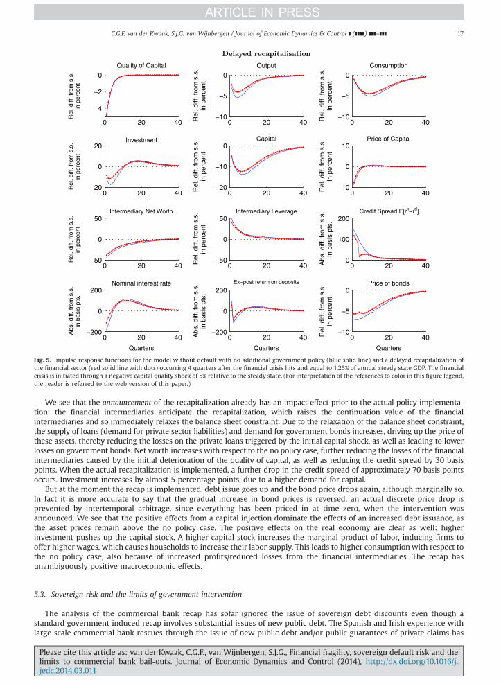
Fig. 5. Impulse response functions for the model without default with no additional government policy (blue solid line) and a delayed recapitalization ofthe financial sector (red solid line with dots) occurring 4 quarters after the financial crisis hits and equal to 1.25% of annual steady state GDP. The financialcrisis is initiated through a negative capital quality shock of 5% relative to the steady state. (For interpretation of the references to color in this figure legend,the reader is referred to the web version of this paper.)
C.G.F. van der Kwaak, S.J.G. van Wijnbergen / Journal of Economic Dynamics & Control ] (]]]]) ]]]–]]] 17
We see that the announcement of the recapitalization already has an impact effect prior to the actual policy implementa-tion: the financial intermediaries anticipate the recapitalization, which raises the continuation value of the financialintermediaries and so immediately relaxes the balance sheet constraint. Due to the relaxation of the balance sheet constraint,the supply of loans (demand for private sector liabilities) and demand for government bonds increases, driving up the price ofthese assets, thereby reducing the losses on the private loans triggered by the initial capital shock, as well as leading to lowerlosses on government bonds. Net worth increases with respect to the no policy case, further reducing the losses of the financialintermediaries caused by the initial deterioration of the quality of capital, as well as reducing the credit spread by 30 basispoints. When the actual recapitalization is implemented, a further drop in the credit spread of approximately 70 basis pointsoccurs. Investment increases by almost 5 percentage points, due to a higher demand for capital.
But at the moment the recap is implemented, debt issue goes up and the bond price drops again, although marginally so.In fact it is more accurate to say that the gradual increase in bond prices is reversed, an actual discrete price drop isprevented by intertemporal arbitrage, since everything has been priced in at time zero, when the intervention wasannounced. We see that the positive effects from a capital injection dominate the effects of an increased debt issuance, asthe asset prices remain above the no policy case. The positive effects on the real economy are clear as well: higherinvestment pushes up the capital stock. A higher capital stock increases the marginal product of labor, inducing firms tooffer higher wages, which causes households to increase their labor supply. This leads to higher consumption with respect tothe no policy case, also because of increased profits/reduced losses from the financial intermediaries. The recap hasunambiguously positive macroeconomic effects.
5.3. Sovereign risk and the limits of government intervention
The analysis of the commercial bank recap has sofar ignored the issue of sovereign debt discounts even though astandard government induced recap involves substantial issues of new public debt. The Spanish and Irish experience withlarge scale commercial bank rescues through the issue of new public debt and/or public guarantees of private claims has
Please cite this article as: van der Kwaak, C.G.F., van Wijnbergen, S.J.G., Financial fragility, sovereign default risk and thelimits to commercial bank bail-outs. Journal of Economic Dynamics and Control (2014), http://dx.doi.org/10.1016/j.jedc.2014.03.011i

C.G.F. van der Kwaak, S.J.G. van Wijnbergen / Journal of Economic Dynamics & Control ] (]]]]) ]]]–]]]18
indicated, however, that such debt financed bank rescues do undermine capital market confidence in the public sector andits debt. This, in turn, may jeopardize the impact of the initial bank rescue action when the same banks hold sovereign debton their balance sheet. To analyze this conflict, we introduce sovereign risk into the model. The specifics of the calibrationstrategies can be found in the appendix. We once again analyze the impact of a recap equal to 1.25% of annual steady stateoutput, and announced at the onset of the financial crisis but implemented 4 quarters later. Fig. 6 compares themacroeconomic responses set against the same experiment but without sovereign risk.
The graphs clearly show that the government default possibility does have a significant effect on the economy. Theannouncement of a recapitalization immediately causes the bond price to drop by an additional 5% with respect to the nodefault case. Investors subsequently anticipate the extra bond issuance necessary for financing the recapitalization, and theaccompanying increase in the sovereign risk discount. This causes additional losses at the financial intermediaries and afurther tightening of the balance sheet constraints of those intermediaries. As a consequence, the cost of capital (requiredreturn) shoots up as the price drops on impact. The effects on the real economy are clear: investment goes down further,pushing down the capital stock, wages go down, and thereby the supply of labor. Consumption eventually decreases morethan in the no default case. Clearly sovereign default risk affects the economy substantially as increased sovereign riskpremia are translated into lower bond prices that further inflict capital losses on the financial intermediaries.
The drop in the bond price clearly shows the limits of government intervention: the bonds are issued to increase bankcapitalization, but their very issuance causes prices to fall, triggering subsequent losses on commercial banks' sovereignasset portfolios that substantially offset the impact of the recap they are financing. The sovereign risk impact of the recapmakes it more difficult to implement effective support measures. This is reminiscent of the failed recapitalization of theSpanish banking sector that the Spanish government (Spanish Ministry of Economic Affairs, 2012) tried to implement inMay 2012, by committing to provide new capital to banks if they could not raise it privately. It was expected that therecapitalization of the Spanish financial sector would relax the debt overhang problems, and create additional room forfinancing the Spanish private sector. Contrary to these expectations, though, bond yields on Spanish government debt shotup and bond prices went down commensurately when the recap was announced, and the Spanish government had to apply
Fig. 6. Impulse response functions comparing the case with no default (blue solid line) and default (red solid line with dots) in case of a delayedrecapitalization of the financial sector of 1.25% of annual steady state GDP that is announced at the start of the financial crisis but implemented 4 quarterslater. Steady state government liabilities are at 80% of annual steady state GDP. The financial crisis is initiated through an initial negative capital quality shockof 5% relative to the steady state. (For interpretation of the references to color in this figure legend, the reader is referred to the web version of this paper.)
Please cite this article as: van der Kwaak, C.G.F., van Wijnbergen, S.J.G., Financial fragility, sovereign default risk and thelimits to commercial bank bail-outs. Journal of Economic Dynamics and Control (2014), http://dx.doi.org/10.1016/j.jedc.2014.03.011i

C.G.F. van der Kwaak, S.J.G. van Wijnbergen / Journal of Economic Dynamics & Control ] (]]]]) ]]]–]]] 19
for a direct financial sector bailout by the EFSF/ESM, whereby the bank risk was taken over by those financial institutions.Our model highlights the importance of the poisonous nexus between banks and sovereigns in times of financial fragility.
6. Conclusion
We have investigated the poisonous interaction between financial fragility, commercial bank holdings of public debt andsovereign risk. We do so by introducing sovereign default risk into a model with financial intermediaries that hold publicdebt in their asset portfolio and are subject to a leverage constraint. We show that the maturity structure of governmentdebt matters a great deal. Issuing more debt as part of a bank recapitalization exercise causes interest rates to rise. But atlonger maturities this leads to larger capital losses for the very banks the debt issue is supposed to recapitalize, and themore so the longer is the average maturity of the sovereign debt outstanding.
We also introduce sovereign default risk and show that the real effects from sovereign default risk are again substantialunder plausible parametrizations of the default process, leading to further difficulties when trying to recapitalize banks aftera financial crisis. Higher debt issuance undermines sovereign credibility and thus leads to larger sovereign debt discounts,further increasing the capital losses on sovereign debt holdings of the banks being intervened. The additional capital lossescause the leverage constraint to tighten more, thereby exacerbating the link between sovereign debt problems and financialfragility, through which sovereign debt problems have a negative impact on the corporate sector: (required) returnsincrease, making finance more expensive, asset prices go down, balance sheet constraints are tightened, with substantialsubsequent negative impact on investment, consumption and output. Obviously, the bond price is most significantlyaffected: the price drop is doubled compared with the case of no sovereign default. This also triggers dynamic problems: thegovernment has to issue more bonds to finance the same intervention, which increases the payments that the governmenthas to make in the future, thereby increasing future debt issuance and default probabilities once again, causing a furtheramplification channel through which bond prices fall even more and losses on bank balance sheets rise again.
The mechanisms we highlighted in this paper bring out the limits to traditional bank intervention when commercialbanks have sovereign bonds on their balance sheets. Capital losses on longer maturity bonds in commercial bank portfolios,through higher interest rates and/or through increased sovereign risk discounts triggered by increased fears of default,undermine the recapitalization for which the bonds are issued to begin with. The link between the sovereign debt-financialfragility nexus and the European debt crisis, and especially the failed Spanish recapitalization attempt in 2012, is clear: ourmodel predicts the increase in sovereign risk discounts and drop in bond prices when announcing a debt financed bankrecapitalization that caused the Spanish government's recapitalization program announced in May 2012 to fail before evenbeing implemented. We explored in this paper a mechanism the literature has abstracted from, the channel is clearlyquantitatively relevant under a fairly standard calibration, suggesting the need and usefulness of further empiricalassessment of macromodels incorporating financial frictions.
Acknowledgment
We thank Keith Kuester of the University of Bonn for many useful suggestions, and for sharing his data and code onsovereign debt exposure of European banks.
Appendix A. Mathematical derivations
A.1. Derivation of structural equations financial intermediaries in presence of sovereign default risk
The introduction of sovereign default risk changes the equations for the financial intermediaries. In this section we show thatthe net worth of an individual intermediary is given by the same expression as the case with no default, except for the fact thatwe replace rt
bby rbnt . Hence we only have to replace rt
bin the equations governing the financial intermediaries by rbnt , and include
the expression for rbnt in the first order conditions. We start by observing that the funds obtained from selling the bonds in periodtþ1, that were purchased in period t, are reduced by 1�Δtþ1, just as the fixed real payment rc per bond is reduced toð1�Δtþ1Þrc. Hence the law of motion for the net worth of an individual intermediary changes into the following equation:
nj;tþ1 ¼ 1þrktþ1
� �qkt s
kj;tþ 1�Δtþ1ð Þrcsbj;tþ 1�Δtþ1ð Þρqbtþ1s
bj;t
� 1þrdtþ1
� �dj;tþng
j;tþ1� ~ngj;tþ1
¼ 1þrktþ1
� �qkt s
kj;tþ 1�Δtþ1ð Þ rcþρqbtþ1
� �sbj;t
� 1þrdtþ1
� �dj;tþng
j;tþ1� ~ngj;tþ1
¼ 1þrktþ1
� �qkt s
kj;tþ 1�Δtþ1ð Þðrcþρq
btþ1Þ
qbtqbt s
bj;t
� 1þrdtþ1
� �dj;tþng
j;tþ1� ~ngj;tþ1
Please cite this article as: van der Kwaak, C.G.F., van Wijnbergen, S.J.G., Financial fragility, sovereign default risk and thelimits to commercial bank bail-outs. Journal of Economic Dynamics and Control (2014), http://dx.doi.org/10.1016/j.jedc.2014.03.011i

C.G.F. van der Kwaak, S.J.G. van Wijnbergen / Journal of Economic Dynamics & Control ] (]]]]) ]]]–]]]20
¼ 1þrktþ1
� �qkt s
kj;tþ 1�Δtþ1ð Þ 1þrbtþ1
� �qbt s
bj;t
� 1þrdtþ1
� �dj;tþng
j;tþ1� ~ngj;tþ1
¼ rktþ1�rdtþ1
� �qkt s
kj;tþðrbntþ1�rdtþ1Þqbt sbj;t
þ 1þrdtþ1
� �nj;tþτntþ1nj;t� ~τntþ1nj;t ;
where rbnt is given by
1þrbnt ¼ 1�Δtð Þ 1þrbt� �
¼ 1�Δtð Þ rcþρqbtqbt�1
!:
We replace rtbby rbnt in the equation for the shadow value of government bonds, and the law of motion of net worth:
νbt ¼ Et Ωtþ1 rbntþ1�rdtþ1
� �h i;
nt ¼ θ rkt �rdt� �
qkt�1skt�1þ rbnt �rdt
� �qbt�1s
bt�1þ 1þrdt
� �nt�1
h iþχpt�1þng
t � ~ngt :
The other equations for the financial intermediaries remain the same.
A.2. Production process
A.2.1. Intermediate goods producersWe remember that period t profits are given by
Πi;t ¼mtatðξtki;t�1Þαh1�αi;t þqkt ð1�δÞξtki;t�1�ð1þrkt Þqkt�1ki;t�1�wthi;t :
The intermediate goods producing firms maximize expected current and future profits using the household's stochasticdiscount factor βsΛt;tþ s (since they are owned by the households), taking all prices as given:
maxfktþ s ;ht þ sg1s ¼ 0
Et ∑1
s ¼ 0βsΛt;tþ sΠi;tþ s
� �:
The first order conditions belonging to this problem are given by
ki;t : Et βΛt;tþ1qkt 1þrktþ1
� �h i¼ Et βΛt;tþ1 αmtþ1yi;tþ1=ki;tþqktþ1ð1�δÞξtþ1
� �h i;
hi;t :wt ¼ ð1�αÞmtyi;t=hi;t :
In equilibrium profits will be zero. By substituting the first order condition for the wage rate into the zero-profit conditionΠi;t ¼ 0, we can find an expression for the ex post return on capital:
rkt ¼ qkt�1
� ��1αmtyi;t=ki;t�1þqkt ð1�δÞξt� �
�1:
Now we rewrite the first order condition for labor and the expression for the ex post return on capital to find the factor demands:
ki;t�1 ¼ αmtyi;t= qkt�1 1þrkt� �
�qkt 1�δð Þξth i
;
hi;t ¼ ð1�αÞmtyi;t=wt :
By substituting the factor demands into the production technology function, we get for the relative intermediate output price mt:
mt ¼ α�αð1�αÞα�1a�1t w1�α
t qkt�1 1þrkt� �
ξ�1t �qkt 1�δð Þ
h iα� �: ð38Þ
A.2.2. Retail firmsRetail firms purchase goods (yi;t) from the intermediate goods producing firms for a nominal price Pt
m, and convert these into
retail goods (yf ;t). These goods are sold for a nominal price Pf ;t to the final goods producer. It takes one intermediate goods unit toproduce one retail good (yi;t ¼ yf ;t). All the retail firms produce a differentiated retail good by assumption, therefore operate in amonopolistically competitive market, and charge a markup over the input price earning them profits ðPf ;t�Pm
t Þyf ;t .Each period, only a fraction 1�ψ of retail firms is allowed to reset their price, while the ψ remaining firms are not
allowed to do so, like in Calvo (1983) and Yun (1996). The firms allowed to adjust prices are randomly selected each period.Once selected, they set prices so as to maximize expected current and future profits, using the stochastic discount factorβsΛt;tþ sðPt=Ptþ sÞ
maxPf ;t
Et ∑1
s ¼ 0ðβψÞsΛt;tþ sðPt=Ptþ sÞ½Pf ;t�Pm
tþ s�� �
yf ;tþ s;
where yf ;t ¼ ðPf ;t=PtÞ� ϵyt is the demand function. yt is the output of the final goods producing firms, and Pt is the generalprice level. Symmetry implies that all firms allowed to reset their prices choose the same new price (Pn
t ). Differentiation with
Please cite this article as: van der Kwaak, C.G.F., van Wijnbergen, S.J.G., Financial fragility, sovereign default risk and thelimits to commercial bank bail-outs. Journal of Economic Dynamics and Control (2014), http://dx.doi.org/10.1016/j.jedc.2014.03.011i
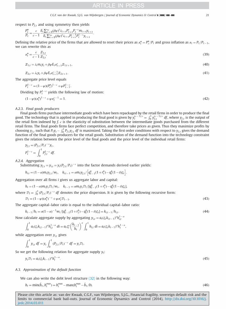
C.G.F. van der Kwaak, S.J.G. van Wijnbergen / Journal of Economic Dynamics & Control ] (]]]]) ]]]–]]] 21
respect to Pf ;t and using symmetry then yields
Pn
t
Pt¼ ϵ
ϵ�1Et∑1
s ¼ 0ðβψÞsλtþ sPϵtþ sP
� ϵt mtþ sytþ s
Et∑1s ¼ 0ðβψÞsλtþ sP
ϵ�1tþ s P
1� ϵt ytþ s
:
Defining the relative price of the firms that are allowed to reset their prices as πnt ¼ Pn
t =Pt and gross inflation as πt ¼ Pt=Pt�1,we can rewrite this as
πnt ¼ϵ
ϵ�1Ξ1;t
Ξ2;t; ð39Þ
Ξ1;t ¼ λtmtytþβψEtπϵtþ1Ξ1;tþ1; ð40Þ
Ξ2;t ¼ λtytþβψEtπϵ�1tþ1Ξ2;tþ1: ð41Þ
The aggregate price level equals
P1� ϵt ¼ ð1�ψÞðPn
t Þ1� ϵþψP1� ϵt�1 :
Dividing by P1� ϵt yields the following law of motion:
ð1�ψÞðπnt Þ1� ϵþψπϵ�1t ¼ 1: ð42Þ
A.2.3. Final goods producersFinal goods firms purchase intermediate goods which have been repackaged by the retail firms in order to produce the final
good. The technology that is applied in producing the final good is given by yðϵ�1Þ=ϵt ¼ R 1
0 yðϵ�1Þ=ϵf ;t df , where yf ;t is the output of
the retail firm indexed by f. ϵ is the elasticity of substitution between the intermediate goods purchased from the differentretail firms. The final goods firms face perfect competition, and therefore take prices as given. Thus they maximize profits bychoosing yf ;t such that Ptyt�
R 10 Pf ;tyf ;t df is maximized. Taking the first order conditions with respect to yf ;t gives the demand
function of the final goods producers for the retail goods. Substitution of the demand function into the technology constraintgives the relation between the price level of the final goods and the price level of the individual retail firms:
yf ;t ¼ ðPf ;t=PtÞ� ϵyt ;
P1� ϵt ¼
Z 1
0P1� ϵf ;t df :
A.2.4. AggregationSubstituting yf ;t ¼ yi;t ¼ ytðPf ;t=PtÞ� ϵ into the factor demands derived earlier yields:
hi;t ¼ ð1�αÞmtyf ;t=wt ; ki;t�1 ¼ αmtyf ;t= qkt�1ð1þrkt Þ�qkt ð1�δÞξth i
:
Aggregation over all firms i gives us aggregate labor and capital:
ht ¼ ð1�αÞmtytDt=wt ; kt�1 ¼ αmtytDt=½qkt�1ð1þrkt Þ�qkt ð1�δÞξt �;where Dt ¼
R 10 ðPf ;t=PtÞ� ϵ df denotes the price dispersion. It is given by the following recursive form:
Dt ¼ ð1�ψÞðπnt Þ� ϵþψπϵtDt�1: ð43ÞThe aggregate capital–labor ratio is equal to the individual capital–labor ratio:
kt�1=ht ¼ αð1�αÞ�1wt=½qkt�1ð1þrkt Þ�qkt ð1�δÞξt � ¼ ki;t�1=hi;t : ð44ÞNow calculate aggregate supply by aggregating yi;t ¼ atðξtki;t�1Þαh1�αi;tZ 1
0atðξtki;t�1Þαh1�αi;t di¼ atξαt
kt�1
ht
� α Z 1
0hi;t di¼ atðξtkt�1Þαh1�α
t ;
while aggregation over yi;t givesZ 1
0yi;t df ¼ yt
Z 1
0ðPf ;t=PtÞ� ϵ df ¼ ytDt :
So we get the following relation for aggregate supply yt:
ytDt ¼ atðξtkt�1Þαh1�αt : ð45Þ
A.3. Approximation of the default function
We can also write the debt level structure (32) in the following way:
bt ¼minð ~bt ; bmaxt Þ ¼ bmax
t �maxðbmaxt � ~bt ;0Þ: ð46Þ
Please cite this article as: van der Kwaak, C.G.F., van Wijnbergen, S.J.G., Financial fragility, sovereign default risk and thelimits to commercial bank bail-outs. Journal of Economic Dynamics and Control (2014), http://dx.doi.org/10.1016/j.jedc.2014.03.011i

Fig. A1. Plot showing the mapping from the no default level of debt ~bt to the actual debt level bt. The solid blue line is the actual mapping, while thedashed red line is an approximation to it, where option pricing formulas have been used. (For interpretation of the references to color in this figure legend,the reader is referred to the web version of this paper.)
C.G.F. van der Kwaak, S.J.G. van Wijnbergen / Journal of Economic Dynamics & Control ] (]]]]) ]]]–]]]22
We can interpret the second term of the new debt level as the payoff of a put option at maturity with underlying process ~bt
and strike price btmax
. The formula for bt, however, does not have a defined derivative at ~bt ¼ bmaxt . Therefore we apply an
approximation for the payoff structure of the put option, and use the option pricing formula, which gives the price of the putoption when time to maturity is equal to T, compounded risk-free interest rate r, and volatility of the underlying process s.This is an approximation to the actual mapping from ~bt to bt, and has in this sense no economic interpretation in our model.The dashed line in Fig. A1 is the approximation to the actual mapping of ~bt to bt. We then get the following approximationfor bt, with Φð�Þ denoting the standard normal CDF, which is indeed continuous:
bt ¼ bmaxt �putt ; ð47Þ
putt ¼ Xe� rTΦð�d2;tÞ�StΦð�d1;tÞ; ð48Þ
d1;t ¼log S=X �þ rþs2
2
� T
sffiffiffiT
p ; ð49Þ
d2;t ¼log S=X �þ r�s2
2
� T
sffiffiffiT
p ; ð50Þ
X ¼ bmaxt ; ð51Þ
St ¼ ~bt : ð52Þ
Appendix B. Supplementary material
An appendix containing the details of the calibration of the default function is available in the Journal's OnlineSupplementary Archive.
Supplementary data associated with this article can be found in the online version at http://dx.doi.org/10.1016/j.jedc.2014.03.011.
References
Acharya, V.V., Drechsler, I., Schnabl, P., 2011. A Pyrrhic Victory? Bank Bailouts and Sovereign Credit Risk. NBER Working Papers 17136.Acharya, V.V., Steffen, S., 2013. Analyzing systemic risk of the European banking sector. In: Fouque, J.P., Langsam, J. (Eds.), Handbook on Systemic Risk,
Cambridge University Press, pp. 247–282. (Chapter 10).Arellano, C., 2008. Default risk and income fluctuations in emerging economies. Am. Econ. Rev. 98 (3), 690–712.
Please cite this article as: van der Kwaak, C.G.F., van Wijnbergen, S.J.G., Financial fragility, sovereign default risk and thelimits to commercial bank bail-outs. Journal of Economic Dynamics and Control (2014), http://dx.doi.org/10.1016/j.jedc.2014.03.011i

C.G.F. van der Kwaak, S.J.G. van Wijnbergen / Journal of Economic Dynamics & Control ] (]]]]) ]]]–]]] 23
Arellano, C., Ramanarayanan, A., 2012. Default and the maturity structure in sovereign bonds. J. Polit. Econ. 120 (2), 187–232.Bernanke, B.S., Gertler, M., Gilchrist, S., 1999. The financial accelerator in a quantitative business cycle framework. In: Taylor, J.B., Woodford, M. (Eds.),
Handbook of Macroeconomics, vol. 1. , Elsevier, pp. 1341–1393. (Chapter 21).Bohn, H., 1998. The behavior of U.S. public debt and deficits. Q. J. Econ. 113 (3), 949–963.Calvo, G.A., 1983. Staggered prices in a utility-maximizing framework. J. Monet. Econ. 12 (3), 383–398.Chatterjee, S., Eyigungor, B., 2012. Maturity, indebtedness, and default risk. Am. Econ. Rev. 102 (6), 2674–2699.Christiano, L.J., Eichenbaum, M., Evans, C.L., 2005. Nominal rigidities and the dynamic effects of a shock to monetary policy. J. Polit. Econ. 113 (1), 1–45.Claessens, S., van Wijnbergen, S., 1993. Secondary market prices and Mexico's Brady deal. Q. J. Econ. 108 (4), 967–982.Cole, H.L., Kehoe, T.J., 2000. Self-fulfilling debt crises. Rev. Econ. Stud. 67 (1), 91–116.Davig, T., Leeper, E.M., Walker, T.B., 2011. Inflation and the fiscal limit. Eur. Econ. Rev. 55 (1), 31–47.European Banking Authority, 2011. 2011 EU-Wide Stress Test Results. URL: ⟨http://www.eba.europa.eu/risk-analysis-and-data/eu-wide-stress-testing/2011/
results⟩.Eurostat, 2014. Quarterly Government Debt. URL: ⟨http://epp.eurostat.ec.europa.eu/portal/page/portal/eurostat/home/⟩.G20 Leaders, 2012. Los Cabos, Mexico, Press Release. URL: ⟨http://g20mexico.org/images/stories/temp/G20_Leaders_Declaration_2012.pdf⟩.Gertler, M., Karadi, P., 2011. A model of unconventional monetary policy. J. Monet. Econ. 58 (1), 17–34.Gertler, M., Karadi, P., 2013. QE 1 vs. 2 vs. 3. . .: a framework for analyzing large-scale asset purchases as a monetary policy tool. Int. J. Cent. Bank. 9 (1), 5–53.Gertler, M., Kiyotaki, N., 2010. Financial intermediation and credit policy in business cycle analysis. In: Friedman, B.M., Woodford, M. (Eds.), Handbook of
Monetary Economics, vol. 3. , Elsevier, pp. 547–599. (Chapter 11).International Herald Tribune, August 7, 2013. Bank System in Germany is Big Worry for Europe.Kirchner, M., van Wijnbergen, S., 2012. Fiscal Deficits, Financial Fragility, and the Effectiveness of Government Policies. Tinbergen Institute Discussion
Papers 12-0442.Kiyotaki, N., Moore, J., 1997. Credit cycles. J. Polit. Econ. 105 (2), 211–248.Moody's Investors Service, 2012a. Rating Action: Moody's Downgrades Spain's Government Bond Rating to Baa3 from A3, on Review for Further
Downgrade. URL: ⟨https://www.moodys.com/research/Moodys-downgrades-Spains-government-bond-rating-to-Baa3-from-A3-PR_248236⟩.Moody's Investors Service, 2012b. Rating Action: Moody's Downgrades Spanish Banks. URL: ⟨https://www.moodys.com/research/Moodys-downgrades-
Spanish-banks-PR_249316⟩.Occhino, F., Pescatori, A., 2010. Debt overhang and credit risk in a business cycle model. Working Paper 1003, Federal Reserve Bank of Cleveland.Reinhart, C.M., Rogoff, K.S., 2009. The aftermath of financial crises. Am. Econ. Rev. 99 (2), 466–472.Schabert, A., van Wijnbergen, S., 2011. Sovereign Default and the Stability of Inflation Targeting Regimes. Tinbergen Institute Discussion Papers 11-064/2/
DSF20.Spanish Ministry of Economic Affairs, 2012. Spain's Path Towards Stability and Growth. URL: ⟨http://www.thespanisheconomy.com/SiteCollectionDocu
ments/en-gb/Financial%20Sector/Spains%20path%20towards%20stability%20and%20growth.pdf⟩.Woodford, M., 1998. Public Debt and the Price Level. Unpublished manuscript Columbia University.Woodford, M., 2001. Fiscal requirements for price stability. J. Money Credit Bank. 33 (3), 669–728.Yun, T., 1996. Nominal price rigidity, money supply endogeneity, and business cycles. J. Monet. Econ. 37 (2–3), 345–370.
Please cite this article as: van der Kwaak, C.G.F., van Wijnbergen, S.J.G., Financial fragility, sovereign default risk and thelimits to commercial bank bail-outs. Journal of Economic Dynamics and Control (2014), http://dx.doi.org/10.1016/j.jedc.2014.03.011i