Financial Intermediation Chains

in an OTC Market∗

Ji Shen

London School of Economicsshenjitoq@gmail.com

Bin WeiFederal Reserve Bank of Atlanta

bin.wei@atl.frb.org

Hongjun YanYale School of Management

hongjun.yan@yale.edu

May 9, 2015

∗We thank Briana Chang, Nicolae Garleanu, Pete Kyle, Ricardo Lagos, Matt Spiegel,Pierre-Olivier Weill, Randall Wright, and seminar participants at UCLA and Yale for helpfulcomments. The views expressed here are those of the authors and do not necessarily reflectthe views of the Federal Reserve Bank of Atlanta or the Federal Reserve System. The latestversion of the paper is available at http://faculty.som.yale.edu/hongjunyan/.

Financial Intermediation Chainsin an OTC Market

Abstract

More and more layers of intermediaries arise in modern financial markets. What

determines this chain of intermediation? What are the consequences? We analyze

these questions in a stylized search model with an endogenous intermediary sector

and intermediation chains. We show that the chain length and the price dispersion

among inter-dealer trades are decreasing in search cost, search speed, and market

size, but increasing in investors’ trading needs. Using data from the U.S. corporate

bond market, we find evidence broadly consistent with these predictions. Moreover,

as the search speed goes to infinity, our search-market equilibrium does not always

converge to the centralized-market equilibrium. In the case with an intermediary

sector, prices and allocations converge, but the trading volume remains higher than

that in a centralized-market equilibrium. This volume difference goes to infinity when

the search cost approaches zero.

JEL Classification Numbers: G10.

Keywords : Search, Chain, Financial Intermediation.

1 Introduction

Financial intermediation chains appear to be getting longer over time, that is, more

and more layers of intermediaries are involved in financial transactions. For instance,

with the rise of securitization in the modern financial system in the U.S., the process

of channeling funds from savers to investors is getting increasingly complex (Adrian

and Shin (2010)). This multi-layer nature of intermediation not only exists in markets

with relatively high transaction costs and “slow” speeds (e.g., mortgage market), it is

also prevalent in those with small transaction costs and exceptionally “fast” speeds.

For example, the average daily trading volume in the Federal Funds market is more

than ten times the aggregate Federal Reserve balances (Taylor (2001)). The trading

volume in the foreign exchange market appears disproportionately large relative to

international trade. According to the Main Economic Indicators database, the annual

international trade in goods and services is around $4 trillion in 2013. In that same

year, however, the Bank of International Settlement estimates that the daily trading

volume in the foreign exchange market is around $5 trillion.

These examples suggest that the multi-layer nature of intermediation is prevalent

for markets across the board. What determines the chain of intermediation? How

does it respond as the economic environment evolves? What is its influence on asset

prices and investor welfare? To analyze these issues, we need theories that endogenize

the chain of intermediation. The literature so far has not directly addressed these

issues. Our paper attempts to fill this gap.

The full answer to the above questions is likely to be complex and hinges on

a variety of issues (e.g., transaction cost, trading technology, regulatory and legal

environment, firm boundary). As the first step, however, we abstract away from many

of these aspects to analyze a simple model of an over-the-counter (OTC) market, and

assess its predictions empirically.1

In the model, investors have heterogeneous valuations of an asset. Their valuations

change over time, leading to trading needs. When an investor enters the market to

trade, he faces a delay in locating his trading partner. In the mean time, he needs to

pay a search cost each period until he finishes his transaction. Due to the delay and

1OTC markets are enormous. According to the estimate by the Bank for International Settle-ments, the total outstanding OTC derivatives is around 711 trillion dollars in December 2013.

1

search cost, not all investors choose to stay in the market all the time, giving rise to a

role of intermediation. Some investors choose to be intermediaries. They stay in the

market all the time and act as dealers. Once they acquire the asset, they immediately

start searching to sell it to someone who values it more. Similarly, once they sell the

asset, they immediately start searching to buy it from someone who values it less. In

contrast, other investors act as customers : once their trades are executed, they leave

the market to avoid the search cost. We solve the model in closed-form, and the main

implications are the following.

First, when the search cost is lower than a certain threshold, there is an equilibrium

with an endogenous intermediary sector. Investors with intermediate valuations of

the asset choose to become dealers and stay in the market all the time, while others

with high or low valuations choose to be customers, and leave the market once their

transactions are executed. Intuitively, if an investor has a high valuation of an asset,

once he obtains the asset, there is little benefit for him to stay in the market since

the chance of finding someone with an even higher valuation is low. Similarly, if

an investor has a low valuation of the asset, once he sells the asset, there is little

benefit for him to stay in the market. In contrast to the above equilibrium, when

the search cost is higher than the threshold, however, there is an equilibrium with no

intermediary. Only investors with very high or low valuations enter the market, and

they leave the market once their trading needs are satisfied. Those with intermediate

valuations have weak trading needs, and choose to stay out of the market to avoid

the search cost.

Second, at each point in time, there is a continuum of prices for the asset. When

a buyer meets a seller, their negotiated price depends on their specific valuations.

The delay in execution in the market makes it possible to have multiple prices for the

asset. Naturally, as the search technology improves, the price dispersion reduces, and

converges to zero when the search technology becomes perfect.

Third, we characterize two equilibrium quantities on the intermediary sector,

which can be easily measured empirically. The first is the dispersion ratio, the price

dispersion among inter-dealer trades divided by the price dispersion among all trades

in the economy.2 The second is the length of the intermediation chain, the average

2For convenience, we refer to the intermediaries in our model as “dealers,” the transactions among

2

number of layers of intermediaries for all customers’ transactions. Intuitively, both

variables reflect the size of the intermediary sector. When more investors choose to

become dealers, the price dispersion among inter-dealer trades is larger (i.e., the dis-

persion ratio is higher), and customers’ transactions tend to go through more layers

of dealers (i.e., the chain is longer).

Our model predicts that both the dispersion ratio and the chain length are de-

creasing in the search cost, the speed of search, and the market size, but are increasing

in investors’ trading frequency. Intuitively, a higher search cost means that fewer in-

vestors find it profitable to be dealers, leading to a smaller intermediary sector and

hence a smaller dispersion ratio and chain length. Similarly, with a higher search

speed or a larger market size, intermediation is less profitable because customers can

find alternative trading partners more quickly. This leads to a smaller intermediary

sector (relative to the market size). Finally, when investors need to trade more fre-

quently, the higher profitability attracts more dealers and so increases the size of the

intermediary sector.

We test these predictions using data from the U.S. corporate-bond market. The

Trade Reporting and Compliance Engine (TRACE) database records transaction

prices, and identifies traders as “dealers” and “customers.” This allows us to construct

the dispersion ratio and chain length. There is substantial cross-sectional variation

in both variables. The dispersion ratio ranges from 0 to 1, while chain length is 1 at

the first percentile and is 7 at the 99th percentile.

We run Fama-MacBeth regressions of the dispersion ratio and chain length of a

corporate bond on proxies for search cost, market size, the frequency of investors’

trading needs. Our evidence is broadly consistent with the model predictions. For

example, we find that investment-grade bonds tend to have larger dispersion ratios

and longer intermediation chains than other bonds. Our regressions suggest that,

on average, relative to other bonds, investment-grade bonds’ price dispersion ratio is

larger by 0.007 (t = 2.62), and their chain length is longer by 0.245 (t = 32.17). If

one takes the interpretation that it is less costly to make market for investment-grade

bonds than for other bonds (i.e., the search cost is lower for investment-grade bonds),

then this evidence is consistent with our model prediction that the dispersion ratio

dealers as “inter-dealer trades.”

3

and chain length are decreasing in search cost. We also include in our regressions five

other variables as proxies for search cost, the frequency of investors’ trading needs,

and market size. Among all 12 coefficients, 11 are highly significant and consistent

with our model predictions.3

Fourth, when the search technology approaches perfection, the search-market equi-

librium does not always converge to a centralized-market equilibrium. Specifically, in

the case without intermediary (i.e., the search cost is higher than a certain thresh-

old), as the search speed goes to infinity, all equilibrium quantities (prices, volumes,

and allocations) converge to their counterparts in the centralized-market equilibrium.

However, in the case with intermediaries (i.e., the search cost is lower than a certain

threshold), as the search speed goes to infinity, all the prices and asset allocations

converge but the trading volume in the search-market equilibrium remains higher

than that in the centralized-market equilibrium. Moreover, this difference in volume

is larger if the search cost is smaller, and converges to infinity when the search cost

goes to 0.

Intuitively, in the search market, intermediaries act as “middlemen” and generate

“excess” trading. As noted earlier, when the search speed increases, the intermediary

sector shrinks. However, thanks to the faster search speed, each dealer executes more

trades, and the total excess trading volume is higher. As the search speed goes to

infinity, the trading volume in the search market remains significantly higher than that

in a centralized market. Moreover, the volume difference increases when the search

cost becomes smaller because a smaller search cost implies a larger intermediary

sector, which leads to a higher excess trading volume in the search market.

This insight sheds light on why a centralized-market model has trouble explaining

trading volume, especially in an environment with a small transaction cost. We

argue that even for the U.S. stock market, it seems plausible that some aspects of

the market are better captured by a search model. For example, the cheaper and

faster trading technology in the last a few decades made it possible for investors to

exploit many high frequency opportunities that used to be prohibitive. Numerous

trading platforms were set up to compete with main exchanges; hedge funds and

3The only exception is the coefficient for issuance size in the price dispersion ratio regression. Asexplained later, we conjecture that this is due to dealers’ inventory capacity constraint, which is notconsidered in our model.

4

especially high-frequency traders directly compete with traditional market makers.

The increase in turnover in the stock market in the last a few decades was likely to

be driven partly by these “intermediation” trades.

Finally, the relation between dispersion ratio, chain length and investors’ welfare

is ambiguous. As noted earlier, a higher dispersion ratio and longer chain may be

due to a lower search cost. In this case, they imply higher investors welfare. On

the other hand, they may be due to a slower search speed. In that case, they imply

lower investors welfare. Hence, the dispersion ratio and chain length are not clear-cut

welfare indicators.

1.1 Related literature

Our paper belongs to the recent literature that analyzes over-the-counter (OTC) mar-

kets in the search framework developed by Duffie, Garleanu, and Pedersen (2005).

This framework has been extended to include risk-averse agents (Duffie, Garleanu,

and Pedersen (2007)), unrestricted asset holdings (Lagos and Rocheteau (2009)). It

has also been adopted to analyze a number of issues, such as security lending (Duffie,

Garleanu, and Pedersen (2002)), liquidity provision (Weill (2007)), on-the-run pre-

mium (Vayanos and Wang (2007), Vayanos and Weill (2008)), cross-sectional returns

(Weill (2008)), portfolio choices (Garleanu (2009)), liquidity during a financial cri-

sis (Lagos, Rocheteau, and Weill (2011)), price pressure (Feldhutter (2012)), order

flows in an OTC market (Lester, Rocheteau, and Weill (2014)), commercial aircraft

leasing (Gavazza 2011), high frequency trading (Pagnotta and Philippon (2013)), the

roles of benchmarks in OTC markets (Duffie, Dworczak, and Zhu (2014)), adverse

selection and repeated contacts in opaque OTC markets (Zhu (2012)) the effect of

the supply of liquid assets (Shen and Yan (2014)) as well as the interaction between

corporate default decision and liquidity (He and Milbradt (2013)). Another literature

follows Kiyotaki and Wright (1993) to analyze the liquidity value of money. In partic-

ular, Lagos and Wright (2005) develop a tractable framework that has been adopted

to analyze liquidity and asset pricing (e.g., Lagos (2010), Lester, Postlewaite, and

Wright (2012), and Li, Rocheteau, and Weill (2012), Lagos and Zhang (2014)). Tre-

jos and Wright (2014) synthesize this literature with the studies under the framework

of Duffie, Garleanu, and Pedersen (2005).

5

Our paper is related to the literature on the trading network of financial markets,

see, e.g., Gofman (2010), Babus and Kondor (2012), Malamud and Rostek (2012).

Atkeson, Eisfeldt, and Weill (2014) analyze the risk-sharing and liquidity provision in

an endogenous core-periphery network structure. Neklyudov (2014) analyzes a search

model with investors with heterogeneous search speeds to study the implications on

the network structure.

Intermediation has been analyzed in the search framework (e.g., Rubinstein and

Wolinsky (1987), and more recently Wright and Wong (2014), Nosal Wong andWright

(2015)). However, the literature on financial intermediation chains has been recent.

Adrian and Shin (2010) document that the financial intermediation chains are be-

coming longer in the U.S. during the past a few decades. Li and Schurhoff (2012)

document the network structure of the inter-dealer market for municipal bonds. Glode

and Opp (2014) focuses on the role of intermediation chain in reducing adverse se-

lection. Afonso and Lagos (2015) analyze an OTC market for Federal Funds. The

equilibrium in their model features an intermediation chain, although they do not

focus on its property. The model that is closest to ours is Hugonnier, Lester, and

Weill (2014). They analyze a model with investors with heterogenous valuations,

highlighting that heterogeneity magnifies the impact of search frictions. Our paper

is different in that, in order to analyze intermediation, we introduce search cost and

derive the intermediary sector, price dispersion ratio, and the intermediation chain,

and also conduct empirical analysis of the intermediary sector.

The rest of the paper is as follows. Section 2 describes the model and its equi-

librium. Section 3 analyzes the price dispersion and intermediation chain. Section 4

contrasts the search market equilibrium with a centralized market equilibrium. Sec-

tion 5 tests the empirical predictions. Section 6 concludes. All proofs are in the

appendix.

2 Model

Time is continuous and goes from 0 to ∞. There is a continuum of investors, and the

measure of the total population is N . They have access to a riskless bank account

with an interest rate r. There is an asset, which has a total supply of X units with

6

X < N . Each unit of the asset pays $1 per unit of time until infinity. The asset is

traded at an over-the-counter market.

Following Duffie, Garleanu, and Pedersen (2005), we assume the matching tech-

nology as the following. Let Nb and Ns be the measures of buyers and sellers in the

market, both of which will be determined in equilibrium. A buyer meets a seller at the

rate λNs, where λ > 0 is a constant. That is, during [t, t+ dt) a buyer meets a seller

with a probability λNsdt. Similarly, a seller meets a buyer at the rate λNb. Hence,

the probability for an investor to meet his partner is proportional to the population

size of the investors on the other side of the market. The total number of matched

pairs per unit of time is λNsNb. The search friction reduces when λ increases, and

disappears when λ goes to infinity.

Investors have different types, and their types may change over time. If an in-

vestor’s current type is ∆, he derives a utility 1 + ∆ when receiving the $1 coupon

from the asset. One interpretation for a positive ∆ is that some investors, such as

insurance companies, have a preference for long-term bonds, as modeled in Vayanos

and Vila (2009). Another interpretation is that some investors can benefit from using

those assets as collateral and so value them more, as discussed in Bansal and Coleman

(1996) and Gorton (2010). An interpretation of a negative ∆ can be that the investor

suffers a liquidity shock and so finds it costly to carry the asset on his balance sheet.

We assume that ∆ can take any value in a closed interval. Without loss of generality,

we normalize the interval to[0,∆

].

Each investor’s type changes independently with intensity κ. That is, during

[t, t+ dt), with a probability κdt, an investor’s type changes and is independently

drawn from a random variable, which has a probability density function f (·) on the

support[0,∆

], with f (∆) < ∞ for any ∆ ∈

[0,∆

]. We use F (·) to denote the

corresponding cumulative distribution function.

Following Duffie, Garleanu, and Pedersen (2005), we assume each investor can

hold either 0 or 1 unit of the asset. That is, an investor can buy 1 unit of the asset

only if he currently does not have the asset, and can sell the asset only if he currently

has it.

There is a search cost of c per unit of time, with c ≥ 0. That is, when an investor

searches to buy or sell in the market, he incurs a cost of cdt during [t, t + dt). All

7

investors are risk-neutral and share the same time discount rate r. An investor’s

objective function is given by

supθτ

Et

[∫∞

t

e−r(τ−t) (θτ (1 + ∆τ )dτ − c1τdτ − Pτdθτ )

],

where θτ ∈ {0, 1} is the investor’s holding in the asset at time τ ; ∆τ is the investor’s

type at time τ ; 1τ is an indicator variable, which is 1 if the investor is searching in

the market to buy or sell the asset at time τ , and 0 otherwise; and Pτ is the asset’s

price that the investor faces at time τ and will be determined in equilibrium.

2.1 Investors’ choices

Since we will focus on the steady-state equilibrium, the value function of a type-∆

investor with an asset holding θt at time t can be denoted as

V (θt,∆) ≡ supθτ

Et

[∫∞

t

e−r(τ−t) (θτ (1 + ∆τ )dτ − c1τdτ − Pτdθτ )

].

A non-owner (whose θt is 0) has two choices: search to buy the asset or stay inactive.

We use Vn(∆) to denote the investor’s expected utility if he chooses to stay inactive,

and follows the optimal strategy after his type changes. Similarly, we use Vb(∆) to

denote the investor’s expected utility if he searches to buy the asset, and follows the

optimal strategy after he obtains the asset or his type changes. Hence, by definition,

we have

V (0,∆) = max(Vn(∆), Vb(∆)). (1)

An asset owner (whose θt is 1) has two choices: search to sell the asset or stay

inactive. We use Vh(∆) to denote the investor’s expected utility if he chooses to be an

inactive holder, and follows the optimal strategy after his type changes. Similarly, we

use Vs(∆) to denote the investor’s expected utility if he searches to sell, and follows

the optimal strategy after he sells his asset or his type changes. Hence, we have

V (1,∆) = max(Vh(∆), Vs(∆)). (2)

We will verify later that in equilibrium, equation (1) implies that a non-owner’s

optimal choice is given by{

stay out of the market if ∆ ∈ [0,∆b),search to buy the asset if ∆ ∈ (∆b,∆],

(3)

8

where the cutoff point ∆b will be determined in equilibrium. A type-∆b non-owner is

indifferent between staying out of the market and searching to buy the asset. Note

that due to the search friction, a buyer faces delay in his transaction. In the meantime,

his type may change, and he will adjust his action accordingly. Similarly, equation

(2) implies that an owner’s optimal choice is

{search to sell his asset if ∆ ∈ [0,∆s),stay out of the market if ∆ ∈ (∆s,∆],

(4)

where the ∆s will be determined in equilibrium. A type-∆s owner of the asset is

indifferent between the two actions. A seller faces potential delay in his transaction.

In the meantime, if his type changes, he will adjust his action accordingly. If an

investor succeeds in selling his asset, he becomes a non-owner and his choices are

then described by equation (3).

Suppose a buyer of type x ∈[0,∆

]meets a seller of type y ∈

[0,∆

]. The surplus

from the transaction is

S (x, y) = [V (1, x) + V (0, y)]︸ ︷︷ ︸total utility after trade

− [V (0, x) + V (1, y)]︸ ︷︷ ︸total utility before trade

. (5)

The pair can agree on a transaction if and only if the surplus is positive. We assume

that the buyer has a bargaining power η ∈ (0, 1), i.e., the buyer gets η of the surplus

from the transaction, and the price is given by

P (x, y) = V (1, x)− V (0, x)− ηS(x, y), if and only if S(x, y) > 0. (6)

The first two terms on the right hand side reflect the value of the asset to the buyer:

the increase in the buyer’s expected utility from obtaining the asset. Hence, the above

equation implies that the transaction improves the buyer’s utility by ηS(x, y).

We conjecture, and verify later, that when a buyer and a seller meet in the market,

the surplus is positive if and only if the buyer’s type is higher than the seller’s:

S (x, y) > 0 if and only if x > y. (7)

That is, when a pair meets, a transaction occurs if and only if the buyer’s type is

higher than the seller’s type. With this conjecture, we obtain investors’ optimality

9

condition in the steady state as the following.

Vh (∆) =1 + ∆ + κE [max {Vh (∆

′) , Vs (∆′)}]

κ + r, (8)

Vs (∆) =1 + y − c

κ+ r+

λ (1− η)

κ+ r

∫ ∆

∆

S (x,∆)µb (x) dx+κE [max {Vh (∆

′) , Vs (∆′)}]

κ+ r,(9)

Vn (∆) =κE [max {Vn (∆

′) , Vb (∆′)}]

κ+ r, (10)

Vb (∆) = −c

κ+ r+

λη

κ+ r

∫ ∆

0

S (∆, x)µs (x) dx+κE [max {Vb (∆) , Vn}]

κ+ r, (11)

where ∆′ is a random variable with a PDF of f(·).

2.2 Intermediation

Decision rules (3) and (4) determine whether intermediation arises in equilibrium.

There are two cases. In the first case, ∆b ≥ ∆s, there is no intermediation. When an

investor has a trading need, he enters the market. Once his transaction is executed,

he leaves the market and stays inactive. In the other case ∆b < ∆s, however, some

investors choose to be intermediaries in equilibrium. If they are non-owners, they

search in the market to buy the asset. Once they receive the asset, however, they

immediately search in the market to sell the asset. For convenience, we call them

“dealers.”

Details are illustrated in Figure 1. Panel A is for the case without intermediation,

i.e., ∆b ≥ ∆s. If an asset owner’s type is below ∆s, as in the upper-left box, he

enters the market to sell his asset. If successful, he becomes a non-owner and chooses

to be inactive since his type is below ∆b, as in the upper-right box. Similarly, if a

non-owner’s type is higher than ∆b, as in the lower-right box, he enters the market to

buy the asset. If successful, he becomes an owner and chooses to be inactive because

his type is above ∆s, as in the lower-left box.

The dashed arrows in the diagram illustrate investors’ chooses to enter or exit the

market when their types change. Suppose, for example, an owner with a type below

∆s is searching in the market to sell his asset, as in the upper-left box. Before he

meets a buyer, however, if his type changes and becomes above ∆s, he will exit the

market and become an inactive owner in the lower-left box. Finally, note that all

investors in the interval (∆s,∆b) are inactive regardless of their asset holdings.

10

Panel B illustrates the case with intermediation, i.e., ∆b < ∆s. As in Panel A,

asset owners with types below ∆s enter the market to sell their assets. However, they

have two different motives. If a seller’s type is in [0,∆b), as in the upper-left box,

after selling the asset, he will leave the market and become an inactive non-owner in

the upper-right box. For convenience, we call this investor a “true seller.” This is

to contrast with those sellers whose types are in (∆b,∆s), as in the middle-left box.

We call them “intermediation sellers,” because once they sell their assets and become

non-owners (i.e., move to the middle-right box), they immediately search to buy the

asset in the market since their types are higher than ∆b. Similarly, we call non-owners

with types in (∆s,∆] “true buyers” and those with types in (∆b,∆s) “intermediation

buyers.”

In the intermediation region (∆b,∆s), investors always stay in the market. If they

are asset owners, they search to sell their assets. Once they become non-owners,

however, they immediately start searching to buy the asset. They buy the asset from

those with low types and sell it to those with high types, and make profits from their

intermediation services.

What determines whether intermediation arises in equilibrium? Intuitively, a key

determinant is the search cost c. Investors are only willing to become intermediaries

when the expected trading profit is enough to cover the search cost. We will see

later that the intermediation equilibrium arises if c < c∗, and the no-intermediation

equilibrium arises if c ≥ c∗, where c∗ is given by equation (72) in the appendix.

2.3 Demographic analysis

We will first focus on the intermediation equilibrium case, and then analyze the no-

intremediation case in Section 4.3. Due to the changes in ∆ and his transactions in

the market, an investor’s status (type ∆ and asset holding θ) changes over time. We

now describe the evolution of the population sizes of each group of investors. Since

we will focus on the steady-state equilibrium, we will omit the time subscript for

simplicity.

We use µb(∆) to denote the density of buyers, that is, buyers’ population size in the

region (∆,∆+d∆) is µb(∆)d∆. Similarly, we use µn(∆), µs(∆), and µh(∆) to denote

the density of inactive non-owners, sellers, and inactive asset holders, respectively.

11

In the steady state, the cross-sectional distribution of investors’ type is given

by the probability density function f (∆). Hence, the total investor population in

(∆,∆ + d∆) is Nf (∆) d∆. Hence, the following accounting identity holds for any

∆ ∈[0,∆

]:

µs (∆) + µb (∆) + µn (∆) + µh (∆) = Nf (∆) . (12)

Decision rules (3) and (4) imply that for any ∆ ∈ (∆s,∆],

µn (∆) = µs (∆) = 0. (13)

In the steady state, the group size of inactive holders remains a constant over

time, implying that for any ∆ ∈ (∆s,∆],

κµh (∆) = κXf (∆) + λNsµb (∆) . (14)

The left hand aside of the above equation is the “outflow” from the group of inactive

holders: The measure of inactive asset holders in interval (∆,∆+ d∆) is µh (∆) d∆.

During [t, t+ dt), a fraction κdt of them experience changes in their types and leave

the group. Hence, the total outflow is κµh (∆) d∆dt. The right hand side of the above

equation is the “inflow” to the group: A fraction κdt of asset owners, who have a

measure of X , experience type shocks and κXf (∆) d∆dt investors’ new types fall

in the interval (∆,∆ + d∆). This is captured by the first term in the right hand

side of (14). The second term reflects the inflow of investors due to transactions.

When buyers with types in (∆,∆+d∆) acquire the asset, they become inactive asset

holders, and the size of this group is λNsµb (∆) d∆dt. Similarly, for any ∆ ∈ [0,∆b),

we have

µb (∆) = µh (∆) = 0, (15)

κµn (∆) = κ (N −X) f (∆) + λNbµs (∆) . (16)

For any ∆ ∈ (∆b,∆s), we have

µn (∆) = µh (∆) = 0, (17)

κµs (∆) = κXf (∆)− λµs (∆)

∫ ∆

∆

µb (x) dx+ λµb (∆)

∫ ∆

0

µs (x) dx. (18)

12

2.4 Equilibrium

Definition 1 The steady-state equilibrium with intermediation consists of two cutoff

points ∆b and ∆s, with 0 < ∆b < ∆s < ∆, the distributions of investor types (µb (∆),

µs (∆), µn (∆), µh (∆)), and asset prices P (x, y), such that

• the asset prices P (x, y) are determined by (6),

• the implied choices (3) and (4) are optimal for all investors,

• the implied sizes of each group of investors remain constants over time and

satisfy (12)–(18),

• market clears: ∫ ∆

0

[µs(∆) + µh(∆)] d∆ = X. (19)

Theorem 1 If c < c∗, where c∗ is given by equation (72), there exists a unique steady-

state equilibrium with ∆b < ∆s. The value of ∆b is given by the unique solution to

c =λκηX

[κ+ r + λNb (1− η)] (κ+ λNb)

∫ ∆b

0

F (x) dx, (20)

the value of ∆s is given by the unique solution to

c =λκ (1− η) (N −X)

(κ+ r + ληNs) (κ+ λNs)

∫ ∆

∆s

[1− F (x)] dx, (21)

where Nb and Ns are given by (54) and (52). Investors’ distributions are given by

equations (44)–(51). When a type-x buyer (x ∈ (∆b,∆]) and a type-y seller (y ∈

[0,∆s)) meet in the market, they will agree to trade if and only if x > y, and their

negotiated price is given by (6), with the value function V (·, ·) given by (67)–(70).

This theorem shows that when the cost of search is smaller than c∗, there is a unique

intermediation equilibrium. Investors whose types are in the interval (∆b,∆s) choose

to be dealers. They search to buy the asset if they do not own it. Once they obtain

the asset, however, they immediately start searching to sell it. They make profits

from the differences in purchase and sale prices to compensate the search cost they

incur. In contrast to these intermediaries, sellers with a type ∆ ∈ [0,∆s) and buyers

13

with a type ∆ ∈ (∆b,∆] are true buyers and true sellers, and they leave the market

once they finish their transactions.

The difficulty in constructing the equilibrium lies in the fact that investors’ type

distributions (µb (∆) , µs (∆) , µn (∆) , µh (∆)) determine the speed with which in-

vestors meet their trading partners, which in turn determines investors’ type dis-

tributions. The equilibrium is the solution to this fixed-point problem.4 The above

theorem shows that the distributions can be computed in closed-form, making the

analysis of the equilibrium tractable.

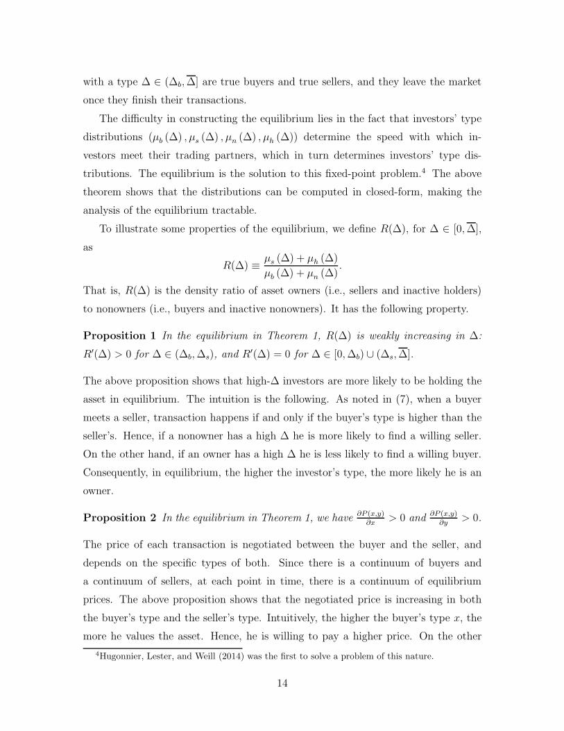
To illustrate some properties of the equilibrium, we define R(∆), for ∆ ∈ [0,∆],

as

R(∆) ≡µs (∆) + µh (∆)

µb (∆) + µn (∆).

That is, R(∆) is the density ratio of asset owners (i.e., sellers and inactive holders)

to nonowners (i.e., buyers and inactive nonowners). It has the following property.

Proposition 1 In the equilibrium in Theorem 1, R(∆) is weakly increasing in ∆:

R′(∆) > 0 for ∆ ∈ (∆b,∆s), and R′(∆) = 0 for ∆ ∈ [0,∆b) ∪ (∆s,∆].

The above proposition shows that high-∆ investors are more likely to be holding the

asset in equilibrium. The intuition is the following. As noted in (7), when a buyer

meets a seller, transaction happens if and only if the buyer’s type is higher than the

seller’s. Hence, if a nonowner has a high ∆ he is more likely to find a willing seller.

On the other hand, if an owner has a high ∆ he is less likely to find a willing buyer.

Consequently, in equilibrium, the higher the investor’s type, the more likely he is an

owner.

Proposition 2 In the equilibrium in Theorem 1, we have ∂P (x,y)∂x

> 0 and ∂P (x,y)∂y

> 0.

The price of each transaction is negotiated between the buyer and the seller, and

depends on the specific types of both. Since there is a continuum of buyers and

a continuum of sellers, at each point in time, there is a continuum of equilibrium

prices. The above proposition shows that the negotiated price is increasing in both

the buyer’s type and the seller’s type. Intuitively, the higher the buyer’s type x, the

more he values the asset. Hence, he is willing to pay a higher price. On the other

4Hugonnier, Lester, and Weill (2014) was the first to solve a problem of this nature.

14

hand, the higher the seller’s type y, the less eager he is in selling the asset. Hence,

only a higher price can induce him to sell.

3 Intermediation Chain and Price Dispersion

If a true buyer and a true seller meet in the market, the asset is transferred without

going through an intermediary. On other occasions, however, transactions may go

through multiple dealers. For example, a type-∆ dealer may buy from a true seller,

whose type is in [0,∆b), or from another dealer whose type is lower than ∆. Then,

he may sell the asset to a true buyer, whose type is in (∆s,∆], or to another dealer

whose type is higher than ∆. Hence, for an asset to be transferred from a true seller

to a true buyer, it may go through multiple dealers.

What is the average length of the intermediation chain in the economy? To analyze

this, we first compute the aggregate trading volumes for each group of investors. We

use TVcc to denote the total number of shares of the asset that are sold from a true

seller to a true buyer (i.e., “customer to customer”) per unit of time. Similarly, we

use TVcd, TVdd, and TVdc to denote the numbers of shares of the asset that are sold,

per unit of time, from a true seller to a dealer (i.e., “customer to dealer”), from a

dealer to another (i.e., “dealer to dealer”), and from a dealer to a true buyer (i.e.,

“dealer to customer”), respectively.

To characterize these trading volumes, we denote Fb(∆) and Fs(∆), for ∆ ∈ [0,∆],

as

Fb(∆) ≡

∫ ∆

0

µb(x)dx,

Fs(∆) ≡

∫ ∆

0

µs(x)dx.

That is, Fb(∆) is the population size of buyers whose types are below ∆, and Fs(∆)

is population size of sellers whose types are below ∆.

15

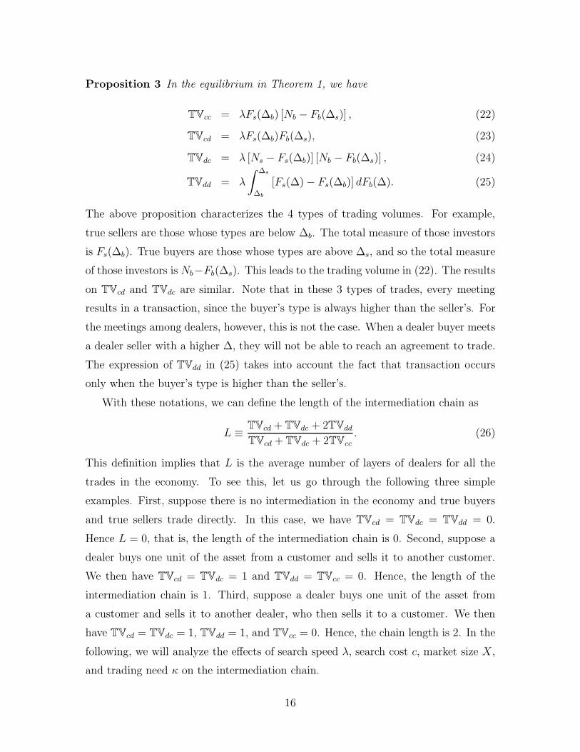
Proposition 3 In the equilibrium in Theorem 1, we have

TVcc = λFs(∆b) [Nb − Fb(∆s)] , (22)

TVcd = λFs(∆b)Fb(∆s), (23)

TVdc = λ [Ns − Fs(∆b)] [Nb − Fb(∆s)] , (24)

TVdd = λ

∫ ∆s

∆b

[Fs(∆)− Fs(∆b)] dFb(∆). (25)

The above proposition characterizes the 4 types of trading volumes. For example,

true sellers are those whose types are below ∆b. The total measure of those investors

is Fs(∆b). True buyers are those whose types are above ∆s, and so the total measure

of those investors is Nb−Fb(∆s). This leads to the trading volume in (22). The results

on TVcd and TVdc are similar. Note that in these 3 types of trades, every meeting

results in a transaction, since the buyer’s type is always higher than the seller’s. For

the meetings among dealers, however, this is not the case. When a dealer buyer meets

a dealer seller with a higher ∆, they will not be able to reach an agreement to trade.

The expression of TVdd in (25) takes into account the fact that transaction occurs

only when the buyer’s type is higher than the seller’s.

With these notations, we can define the length of the intermediation chain as

L ≡TVcd + TVdc + 2TVdd

TVcd + TVdc + 2TVcc

. (26)

This definition implies that L is the average number of layers of dealers for all the

trades in the economy. To see this, let us go through the following three simple

examples. First, suppose there is no intermediation in the economy and true buyers

and true sellers trade directly. In this case, we have TVcd = TVdc = TVdd = 0.

Hence L = 0, that is, the length of the intermediation chain is 0. Second, suppose a

dealer buys one unit of the asset from a customer and sells it to another customer.

We then have TVcd = TVdc = 1 and TVdd = TVcc = 0. Hence, the length of the

intermediation chain is 1. Third, suppose a dealer buys one unit of the asset from

a customer and sells it to another dealer, who then sells it to a customer. We then

have TVcd = TVdc = 1, TVdd = 1, and TVcc = 0. Hence, the chain length is 2. In the

following, we will analyze the effects of search speed λ, search cost c, market size X ,

and trading need κ on the intermediation chain.

16

3.1 Search cost c

Proposition 4 In the equilibrium in Theorem 1, ∂∆b

∂c> 0 and ∂∆s

∂c< 0, that is, the

total population size of the intermediary sector is decreasing in c.

Intuitively, investors balance the gain from trade against the search cost. The search

cost has a disproportionately large effect on dealers since they stay active in the

market constantly. Hence, when the search cost c increases, fewer investors choose to

be dealers and so the size of the intermediary sector becomes smaller (i.e., the interval

(∆b,∆s) shrinks). Consequently, the smaller intermediary sector leads to a shorter

intermediation chain, as summarized in the following proposition.

Proposition 5 In the equilibrium in Theorem 1, ∂L∂c

< 0, that is, the length of the

financial intermediation chain is decreasing in c.

When c increases to c∗, the interval (∆b,∆s) shrinks to a point and the intermediary

sector disappears. Hence, we have limc→c∗ L = 0. On the other hand, as c decreases,

more investors choose to be dealers, leading to more layers of intermediation and a

longer chain in the economy. What happens when c goes to zero?

Proposition 6 When c goes to 0, in the equilibrium in Theorem 1, the following

holds:

∆b = 0, ∆s = ∆,

Ns = X, Nb = N −X,

L = ∞.

As the search cost c diminishes, the intermediary sector (∆b,∆s) expands. When c

goes to 0, (∆b,∆s) becomes the whole interval (0,∆). That is, all investors (except

zero measure of them at 0 and ∆) are intermediaries, constantly searching in the

market. Hence, Ns = X and Nb = N − X , that is, virtually every asset holder

is trying to sell his asset and every non-owner is trying to buy. Since virtually all

transactions are intermediation trading, the length of the intermediation chain is

infinity.

17

3.2 Search speed λ

Proposition 7 In the equilibrium in Theorem 1, when λ is sufficiently large, ∂∆s−∆b

∂λ<

0, that is, the intermediary sector shrinks when λ increases; ∂L∂λ

< 0, that is, the length

of the financial intermediation chain is decreasing in λ.

The intuition for the above result is the following. As the search technology improves,

a customer has a higher outside option value when he trades with a dealer. This is

because the customer can find an alternative trading partner more quickly, if the

dealer were to turn down the trade. As a result, intermediation is less profitable and

the dealer sector shrinks, leading to a shorter intermediation chain.

3.3 Market size X

To analyze the effect of the market size X , we keep the ratio of investor population

N and asset supply X constant. That is, we let

N = φX, (27)

where φ is a constant. Hence, when the issuance size X changes, the population size

N also changes proportionally. We impose this condition to shut down the effect from

the change in the ratio of asset owners and non-owners in equilibrium.

Proposition 8 In the equilibrium in Theorem 1, under condition (27), when λ is

sufficiently large, ∂∆s−∆b

∂X< 0, that is, the intermediary sector shrinks when the market

size increases; ∂L∂X

< 0, that is, the length of the financial intermediation chain is

decreasing in the size of the market X.

Intuitively, when the market size gets larger, it becomes easier for an investor to

meet his trading partner. Hence, the effect is similar to that from an increase in the

search speed λ. From the intuition in Proposition 7, we obtain that the length of the

financial intermediation chain is decreasing in the size of the market.

3.4 Trading need κ

Proposition 9 In the equilibrium in Theorem 1, when λ is sufficiently large, ∂(∆s−∆b)∂κ

>

0, and ∂L∂κ

> 0, that is, the intermediary sector expands and the length of the inter-

mediation chain increases when the frequency of investors’ trading need increases.

18

The intuition for the above result is as follows. Suppose κ increases, i.e., investors

need to trade more frequently. This makes it more profitable for dealers. Hence, the

intermediary sector expands as more investors choose to become dealers, leading to

a longer intermediation chain.

3.5 Price dispersion

Theorem 1 shows that there is a continuum of prices for the asset in equilibrium.

How is the price dispersion related to search frictions? It seems reasonable to expect

the price dispersion to decrease as the market frictions diminishes. However, this

intuition is not complete, and the relationship between price dispersion and search

frictions is more subtle.

To see this, we use D to denote the price dispersion

D ≡ Pmax − Pmin, (28)

where Pmax and Pmin are the maximum and minimum prices, respectively, among all

prices. Proposition 2 implies that

Pmax = P (∆,∆s), (29)

Pmin = P (∆b, 0). (30)

That is, Pmax is the price for the transaction between a buyer of type ∆ and a seller

of type ∆s. Similarly, Pmin is the price of the transaction between a buyer of type ∆b

and a seller of type 0. The following proposition shows that effect of the search speed

on the price dispersion.

Proposition 10 In the equilibrium in Theorem 1, when λ is sufficiently large, ∂D∂λ

<

0.

The intuition is the following. When the search speed is faster, investors do not

have to compromise as much on prices to speed up their transactions, because they

can easily find alternative trading partners if their current trading partners decided

to walk away from their transactions. Hence, the dispersion across prices becomes

smaller when λ increases.

19

However, the relation between the price dispersion and the search cost c is more

subtle. As the search cost increases, fewer investors participate in the market. On

the one hand, this makes it harder to find a trading partner and so increases the

price dispersion as the previous proposition suggests. There is, however, an opposite

driving force: Less diversity across investors leads to a smaller price dispersion. In

particular, as noted in Proposition 4, ∆s is decreasing in c, that is, when the search

cost increases, only investors with lower types are willing to pay the cost to try to sell

their assets. As noted in (29), this reduces the maximum price Pmax. On the other

hand, when the search cost increases, only investors with higher types are willing to

buy. This increases the minimum price Pmin. Therefore, as the search cost increases,

the second force decreases the price dispersion. The following proposition shows that

the second force can dominate.

Proposition 11 In the equilibrium in Theorem 1, the sign of ∂D∂c

can be either posi-

tive or negative. Moreover, when c is sufficiently small, we have ∂D∂c

< 0.

Price dispersion in OTC markets has been documented in the literature, e.g., Green,

Hollifield, and Schurhoff (2007). Jankowitsch, Nashikkar, and Subrahmanyam (2011)

proposes that price dispersion can be used as a measure of liquidity. Our analysis

in Proposition 10 confirms this intuition that the price dispersion is larger when

the search speed is lower, which can be interpreted as the market being less liquid.

However, Proposition 11 also illustrates the potential limitation, especially in an

environment with a low search cost. It shows that the price dispersion may decrease

when the search cost is higher.

3.6 Price dispersion ratio

To further analyze the price dispersion in the economy, we define dispersion ratio as

DR ≡P dmax − P d

min

Pmax − Pmin

, (31)

where P dmax and P d

min are the maximum and minimum prices, respectively, among

inter-dealer transactions. That is, DR is the ratio of the price dispersion among

inter-dealer transactions to the price dispersion among all transactions.

20

This dispersion ratio measure has two appealing features. First, somewhat surpris-

ingly, it turns out to be easier to measure DR than D. Conceptually, price dispersion

D is the price dispersion at a point in time. When measuring it empirically, how-

ever, we have to compromise and measure the price dispersion during a period of

time (e.g., a month or a quarter), rather than at an instant. As a result, the asset

price volatility directly affects the measure D. In contrast, the dispersion ratio DR

alleviates part of this problem since asset price volatility affects both the numerator

and the denominator. Second, as noted in Proposition 11, the effect of search cost

on the price dispersion is ambiguous. In contrast, our model predictions on the price

dispersion ratio are sharper, as illustrated in the following proposition.

Proposition 12 In the equilibrium in Theorem 1, we have ∂DR∂c

< 0; when λ is

sufficiently large, we have ∂DR∂λ

< 0, ∂DR∂κ

> 0, and under condition (27) we have

∂DR∂X

< 0.

Intuitively, DR is closely related to the size of the intermediary sector. All these

parameters (c, λ,X, and κ) affect DR through their effects on the interval (∆b,∆s).

For example, as noted in Proposition 4, when the search cost c increases, the inter-

mediary sector (∆b,∆s) shrinks, and so the price dispersion ratio DR decreases. The

intuition for the effects of all other parameters (λ,X, and κ) is similar.

In summary, both DR and L are closely related to the size of the intermediary

sector. All the parameters of (c, λ,X, and κ) affect both DR and L through their

effects on the interval (∆b,∆s). Indeed, by comparing the above results with Propo-

sitions 5, 7, 8, and 9, we can see that, for all four parameters (c, λ,X, and κ), the

effects on DR and L have the same sign.

3.7 Welfare

What are the welfare implications from the intermediation chain? For example, is a

longer chain an indication of higher or lower investors’ welfare? Propositions 5–12

have shed some light on this question. In particular, a longer intermediation chain (or

a larger price dispersion ratio) is a sign of a lower c, a lower λ, a higher κ, or a lower

X , which have different welfare implications. Hence, the chain length and dispersion

ratio are not clear-cut indicators of investors’ welfare.

21

For example, a lower c means that more investors would search in equilibrium.

Hence, high-∆ investors can obtain the asset more quickly, leading to higher welfare

for all investors. On the other hand, a lower λ means that investors obtain their

desired asset positions more slowly, leading to lower welfare for investors. Therefore,

if the intermediation chain L becomes longer (or the price dispersion ration DR gets

larger) because of a lower c, it is a sign of higher investor welfare. However, if it is

due to a lower search speed λ, it is a sign of lower investor welfare. A higher κ means

that investors have more frequent trading needs. If L becomes longer (or DR gets

larger) because of a higher κ, holding the market condition constant, this implies that

investors have lower welfare. Finally, if L becomes longer (or DR gets larger) because

of a smaller X , it means that investors execute their trades more slowly, leading to

lower welfare for investors. To formalize the above intuition, we use W to denote the

average expected utility across all investors in the economy. The relation between

investors’ welfare and those parameters is summarized in the following proposition.

Proposition 13 In the equilibrium in Theorem 1, we have ∂W∂c

< 0; when λ is suffi-

ciently large, we have ∂W∂λ

> 0, ∂W∂κ

< 0, and under condition (27) ∂W∂X

> 0.

4 On Convergence

When the search friction disappears, does the search market equilibrium converge to

the equilibrium in a centralized market? Since Rubinstein and Wolinsky (1985) and

Gale (1987), it is generally believed that the answer is yes. This convergence result

is also demonstrated in Duffie, Garleanu, and Pedersen (2005), the framework we

adopted.

However, we show in this section that as the search technology approaches per-

fection (i.e., λ goes to infinity) the search equilibrium does not always converge to a

centralized market equilibrium. In particular, consistent with the existing literature,

the prices and allocation in the search equilibrium converge to their counterparts in

a centralized-market equilibrium, but the trading volume may not.

22

4.1 Centralized market benchmark

Suppose we replace the search market in Section 2 by a centralized market and keep

the rest of the economy the same. That is, investors can execute their transactions

without any delay. The centralized market equilibrium consists of an asset price Pw

and a cutoff point ∆w. All asset owners above ∆w and nonowners below ∆w stay

inactive. Moreover, each nonowner with a type higher than ∆w buys one unit of the

asset instantly and each owner with a type lower than ∆w sells his asset instantly,

such that all investors find their strategies optimal, the distribution of all groups of

investors remain constant over time, and the market clears. This equilibrium is given

by the following proposition.

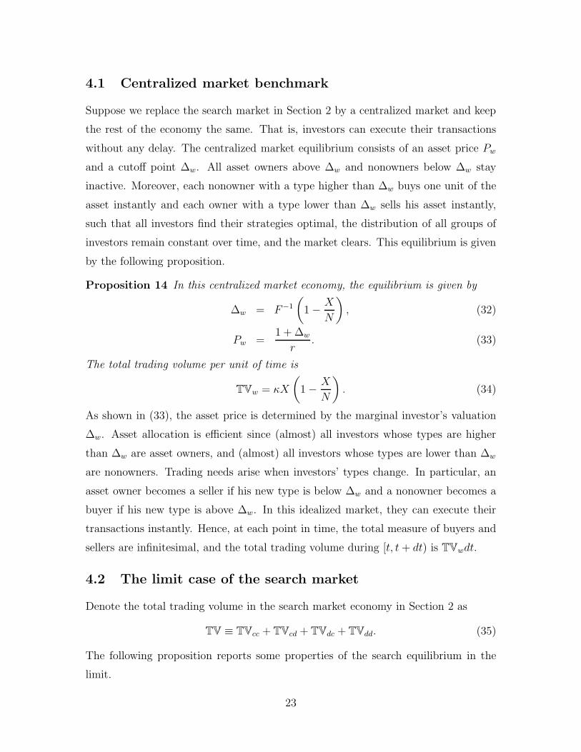
Proposition 14 In this centralized market economy, the equilibrium is given by

∆w = F−1

(1−

X

N

), (32)

Pw =1 +∆w

r. (33)

The total trading volume per unit of time is

TVw = κX

(1−

X

N

). (34)

As shown in (33), the asset price is determined by the marginal investor’s valuation

∆w. Asset allocation is efficient since (almost) all investors whose types are higher

than ∆w are asset owners, and (almost) all investors whose types are lower than ∆w

are nonowners. Trading needs arise when investors’ types change. In particular, an

asset owner becomes a seller if his new type is below ∆w and a nonowner becomes a

buyer if his new type is above ∆w. In this idealized market, they can execute their

transactions instantly. Hence, at each point in time, the total measure of buyers and

sellers are infinitesimal, and the total trading volume during [t, t + dt) is TVwdt.

4.2 The limit case of the search market

Denote the total trading volume in the search market economy in Section 2 as

TV ≡ TVcc + TVcd + TVdc + TVdd. (35)

The following proposition reports some properties of the search equilibrium in the

limit.

23

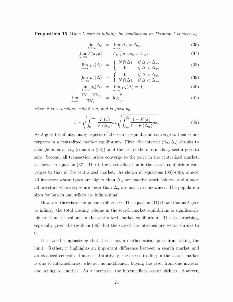
Proposition 15 When λ goes to infinity, the equilibrium in Theorem 1 is given by

limλ→∞

∆b = limλ→∞

∆s = ∆w, (36)

limλ→∞

P (x, y) = Pw for any x < y, (37)

limλ→∞

µh(∆) =

{Nf(∆) if ∆ > ∆w,

0 if ∆ < ∆w,(38)

limλ→∞

µn(∆) =

{0 if ∆ > ∆w,

Nf(∆) if ∆ < ∆w,(39)

limλ→∞

µb(∆) = limλ→∞

µs(∆) = 0, (40)

limλ→∞

TV− TVw

TVw

= logc

c, (41)

where c is a constant, with c > c, and is given by

c =

√∫ ∆w

0

F (x)

F (∆w)dx

√∫ ∆

∆w

1− F (x)

1− F (∆w)dx. (42)

As λ goes to infinity, many aspects of the search equilibrium converge to their coun-

terparts in a centralized market equilibrium. First, the interval (∆b,∆s) shrinks to

a single point at ∆w (equation (36)), and the size of the intermediary sector goes to

zero. Second, all transaction prices converge to the price in the centralized market,

as shown in equation (37). Third, the asset allocation in the search equilibrium con-

verges to that in the centralized market. As shown in equations (38)–(40), almost

all investors whose types are higher than ∆w are inactive asset holders, and almost

all investors whose types are lower than ∆w are inactive nonowners. The population

sizes for buyers and sellers are infinitesimal.

However, there is one important difference. The equation (41) shows that as λ goes

to infinity, the total trading volume in the search market equilibrium is significantly

higher than the volume in the centralized market equilibrium. This is surprising,

especially given the result in (36) that the size of the intermediary sector shrinks to

0.

It is worth emphasizing that this is not a mathematical quirk from taking the

limit. Rather, it highlights an important difference between a search market and

an idealized centralized market. Intuitively, the excess trading in the search market

is due to intermediaries, who act as middlemen, buying the asset from one investor

and selling to another. As λ increases, the intermediary sector shrinks. However,

24

thanks to the faster search technology, each intermediary can execute more trades

such that the total excess trading induced by intermediaries increases with λ despite

the reduction in the size of the intermediary sector. As λ goes to infinity, the trading

volume in the search market remains significantly higher than that in a centralized

market.

As illustrated in (41), the difference between TV and TVw is larger when the search

cost c is smaller, and approaches infinity when c goes to 0. As noted in Proposition 4,

the smaller the search cost c, the larger the intermediary sector. Hence, the smaller

the search cost c, the larger the excess trading generated by middlemen.

These results shed some light on why centralized market models have trouble

explaining trading volume, especially in markets with small search frictions. Even

in the well-developed stock market in the U.S., some trading features are perhaps

better captured by a search model. It is certainly quick for most investors to trade in

the U.S. stock market. However, the cheaper and faster technology makes it possible

for investors to exploit opportunities that were prohibitive with a less developed

technology. Indeed, over the past a few decades, numerous trading platforms were

set up to compete with main exchanges; hedge funds and especially high-frequency

traders directly compete with traditional market makers. It seems likely that the

increase in turnover in the stock market in the past a few decades was driven partly

by the decrease in the search frictions in the market. Intermediaries, such as high

frequency traders, execute a large volume of trades to exploit opportunities that used

to be prohibitive.

In summary, our analysis suggests that a centralized market model captures the

behavior of asset prices and allocations when market frictions are small. However, it

is not well-suited for analyzing trading volume, even in a market with a fast search

speed, especially in the case when the search cost is small.

4.3 Equilibrium without Intermediation

Our discussion so far has focused on the case c < c∗. We now briefly summarize

the analysis for the other case. As noted in Section 3.1, when c increases to c∗,

the interval (∆b,∆s) shrinks to a point and the intermediary sector disappears. As

one might have expected, intermediaries disappear in the equilibrium for the case of

25

c ≥ c∗.

Similar to the analysis in Section 2, we can construct an equilibrium for the case

c ≥ c∗. The only difference is that as described in Panel A of Figure 1, two cutoff

points ∆b and ∆s are such that ∆b ≥ ∆s. In the equilibrium in Theorem 1, investors

with intermediate valuations become intermediaries and stay in the market all the

time. In contrast, in this case with a higher search cost, investors with intermediate

valuations choose not to participate in the market. Only those with strong trading

motives (buyers with types higher than ∆b and sellers with types lower than ∆s)

are willing to pay the high search cost to participate in the market. In the limit case

where λ goes to infinity, as in Proposition 15, equations (36)–(40) still hold. However,

we now have

limλ→∞

TV = TVw.

This is, as λ goes to infinity, both ∆b and ∆s converge to ∆w. The inactive sector

shrinks to a point. Moreover, the prices, allocation, and the trading volume all con-

verge to their counterparts in a centralized market equilibrium. This result further

confirms our earlier intuition that, in the intermediation equilibrium in Section 2, the

difference between TV and TVw is due to the extra trading generated by intermedi-

aries acting as middlemen.

4.4 Alternative matching functions

Section 4.2 shows that the non-convergence result on volume is due to the fact that

while λ increases, the intermediary sector shrinks but each one can trade more quickly.

The higher trading speed dominates the reduction in the size of the intermediary sec-

tor. One natural question whether this result depends on the special matching func-

tion in our model. As explained in Section 2, for tractability, we adopt the matching

function λNbNs. Does our non-convergence conclusion depend on this assumption?

To examine this, we modify our model to have a more general matching function:

We now assume that the matching function is λQ(Nb, Ns), where Q(·, ·) is homoge-

neous of degree k (k > 0) in Nb and Ns. The matching function in our previous

analysis, λNbNs, is a special case with homogeneity of degree 2. The rest of the

model is kept the same as in Section 2. We construct an intermediation equilibrium

that is similar to the one in Theorem 1, and let λ go to infinity to compare the limit

26

equilibrium with the centralized market equilibrium.

The conclusions based on this general matching function remain the same as those

in Section 4.2. When λ goes to infinity, both the prices and allocation converge to

their counterparts in a centralized market equilibrium, but the trading volume does

not. Interestingly, the trading volume in this generalized model converges to exactly

the same value as in our previous model, and is given by (41).

5 Empirical Analysis

In this section, we conduct empirical tests of the model predictions on the length of the

intermediation chain L and the price dispersion ratio DR. We choose to analyze the

U.S. corporate bond market, which is organized as an OTC market, where dealers and

customers trade bilaterally. Moreover, a large panel dataset is available that makes

it possible to conduct the tests reliably.

5.1 Hypotheses

Our analysis in Section 3 provides predictions on the effects of search cost c, market

size X , trading need κ, and search technology λ. Our empirical analysis will focus

on the cross-sectional relations. Hence, there is perhaps little variation in the search

technology λ across corporate bonds in our sample during 2002–2012. Our analysis

below will focus on the effects of c, X , and κ.

Specifically, we obtain a number of observable variables that can be used as proxies

for these three parameters. Table 1 summarizes the interpretations of our proxies and

model predictions. We use issuance size as a proxy for the market size X . Another

variable that captures the effect of market size is age. The idea is that after a corporate

bond is issued, as time goes by, a larger and larger fraction of the issuance reaches long-

term buy-and-hold investors such as pension funds and insurance companies. Hence,

the active size of the market becomes smaller as the bond age increases. With these

interpretations, Propositions 8 and 12 imply that the intermediation chain length L

and price dispersion ratioDR should be decreasing in the issuance size, but increasing

in bond age.

We use turnover as a proxy for the frequency of investors’ trading need κ. The

27

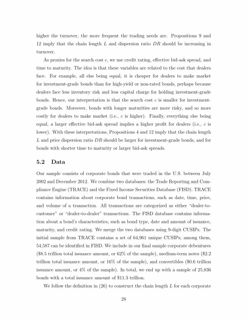
higher the turnover, the more frequent the trading needs are. Propositions 9 and

12 imply that the chain length L and dispersion ratio DR should be increasing in

turnover.

As proxies for the search cost c, we use credit rating, effective bid-ask spread, and

time to maturity. The idea is that these variables are related to the cost that dealers

face. For example, all else being equal, it is cheaper for dealers to make market

for investment-grade bonds than for high-yield or non-rated bonds, perhaps because

dealers face less inventory risk and less capital charge for holding investment-grade

bonds. Hence, our interpretation is that the search cost c is smaller for investment-

grade bonds. Moreover, bonds with longer maturities are more risky, and so more

costly for dealers to make market (i.e., c is higher). Finally, everything else being

equal, a larger effective bid-ask spread implies a higher profit for dealers (i.e., c is

lower). With these interpretations, Propositions 4 and 12 imply that the chain length

L and price dispersion ratio DR should be larger for investment-grade bonds, and for

bonds with shorter time to maturity or larger bid-ask spreads.

5.2 Data

Our sample consists of corporate bonds that were traded in the U.S. between July

2002 and December 2012. We combine two databases: the Trade Reporting and Com-

pliance Engine (TRACE) and the Fixed Income Securities Database (FISD). TRACE

contains information about corporate bond transactions, such as date, time, price,

and volume of a transaction. All transactions are categorized as either “dealer-to-

customer” or “dealer-to-dealer” transactions. The FISD database contains informa-

tion about a bond’s characteristics, such as bond type, date and amount of issuance,

maturity, and credit rating. We merge the two databases using 9-digit CUSIPs. The

initial sample from TRACE contains a set of 64,961 unique CUSIPs; among them,

54,587 can be identified in FISD. We include in our final sample corporate debentures

($8.5 trillion total issuance amount, or 62% of the sample), medium-term notes ($2.2

trillion total issuance amount, or 16% of the sample), and convertibles ($0.6 trillion

issuance amount, or 4% of the sample). In total, we end up with a sample of 25,836

bonds with a total issuance amount of $11.3 trillion.

We follow the definition in (26) to construct the chain length L for each corporate

28

bond during each period, where TVcd + TVdc is the total dealer-to-customer trading

volume and TVdd is the total dealer-to-dealer trading volume during that period. In

our data, TVcc = 0, that is, there is no direct transaction between two customers.

Hence, the chain length is always larger than or equal to 1.

We obtain the history of credit ratings on the bond level from FISD. For each

bond, we construct its credit rating history at the daily frequency: for each day, we

use credit rating by S&P if it is available, otherwise, we use Moody’s rating if it is

available, and use Fitch’s rating if both S&P and Moody’s ratings are unavailable.

In the case that a bond is not rated by any of the three credit rating agencies, we

consider it as “not rated.” We use the rating on the last day of the period to create

a dummy variable “IG”, which equals one if a bond has an investment-grade rating,

and zero otherwise.

To measure the effective bid-ask spread of a bond, denoted as Spread, we follow

Bao, Pan, and Wang (2011) to compute the square root of the negative of the first-

order autocovariance of changes in consecutive transaction prices during the period,

which is based on Roll (1984)’s measure of effective bid-ask spread. Maturity refers

to the time to maturity of a bond, measured in years. We use Age to denote the time

since issuance of a bond, denominated in years, use Size to denote issuance size of a

bond, denominated in million dollars, and use Turnover to denote the total trading

volume of a bond during the period, normalized by its Size.

We follow the definition in equation (31) to construct the price dispersion ratio,

DR, for each bond and time period, where P dmax and P d

min are the maximum and

minimum transaction prices among dealer-to-dealer transactions, and Pmax and Pmin

are the maximum and minimum transaction prices among all transactions.

5.3 Analysis

Table 2 reports the summary statistics for variables measured at the monthly fre-

quency. To rule out extreme outliers, which are likely due to data error, we winsorize

our sample by dropping observations below the 1st percentile and above 99th per-

centile. For the overall sample, the average chain length is 1.73. There is significant

variation. The chain length is 7.00 and 1.00 at the 99th and 1st percentiles, respec-

tively. Investment-grade bonds tend to have longer chains. For example, the average

29

chain length is 1.81 and the 99th percentile is 7.53. The average price dispersion ratio

is 0.50 for the overall sample, and 0.51 for investment-grade bonds. For the overall

sample, the average turnover is 0.08 per month and the average issuance size is $462

million. Investment-grade bonds have a larger average issuance size of $537 million,

and a turnover ratio of 0.07. The effective bid-ask spread is 1.43% for the overall

sample, and 1.32% for the investment-grade subsample. The average bond age is

around 5 years and the time to maturity is around 8 years.

We first run Fama-MacBeth regressions of chain length on the variables in Table

1, and the results are reported in Table 3. As shown in column 1, the signs of all

coefficients are consistent with the model predictions, and all coefficients are highly

significantly different from 0. The coefficient for IG is 0.245 (t = 32.17) implying

that, holding everything else constant, the chain length for investment-grade bonds

is longer than that for other bonds by 0.245 on average. The coefficient for Spread is

0.073, with a t-statistic of 17.17. Hence, when the effective bid-ask spread increases

from the 25th percentile to the 75th percentile, the chain length increases by 0.091

(= 0.073×(1.81−0.56)). With the interpretation that a higher spread implies a lower

cost for dealers, this is consistent our model that the chain length is decreasing in

the search cost. The coefficient for Turnover is 0.199 (t = 11.48), suggesting that the

chain length increases with the frequency of investors’ trading needs. The coefficients

for Size and Age are −0.012 (t = 3.73) and 0.025 (t = 23.92), implying that the

chain length is decreasing in the size of the market. Also consistent with the model

prediction, the coefficient for Maturity is significantly negative.

We then run another Fama-MacBeth regression, using the price dispersion DR

as the dependent variable. Our model predicts that the signs of coefficients for all

the variables should be the same as those in the regression for L. As shown in the

third column of Table 3, five out of the six coefficients have the same sign as those

in the regression for L in column 1. For example, as shown in the third column of

Table 3, the coefficient for IG is 0.007 (t = 2.62) implying that, holding everything

else constant, the price dispersion for investment grade bonds is larger than that for

other bonds by 0.007 on average. Similarly, as implied by our model, the coefficients

for other variables such as Spread, Turnover, Age, and Maturity are all significant

and have the same sign as in the regression for L.

30

The only exception is for Size. Contrary to our model prediction, the coefficient is

significantly positive. Intuitively, our model implies that, for a larger bond, it is easier

to find trading partners. Hence, it is less profitable for dealers, leading to a smaller

intermediary sector, and consequently a shorter intermediation chain and a smaller

price dispersion ratio. However, our evidence is only consistent with the implication

on the chain length, but not the one on the price dispersion ratio. One conjecture

is that our model abstracts away from the variation in transaction size and dealers’

inventory capacity constraints. For example, in our sample, the monthly maximum

transaction size for the largest 10% of the bonds is more than 50 times larger than

that for the smallest 10% of the bonds. When facing extremely large transactions

from customers, with inventory capacity constraints, a dealer may have to offer price

concessions when trading with other dealers, leading to a larger price dispersion ratio.

However, this channel has a much weaker effect on the chain length, which reflects the

average number of layers of intermediation and so is less sensitive to the transactions

of extreme sizes. As a result, our model prediction on the chain length holds but the

prediction on the price dispersion does not.

As a robustness check, we reconstruct all variables at the quarterly frequency

and repeat our analysis. As shown in the second and fourth columns, the results

at the quarterly frequency are similar to those at the monthly frequency. The only

difference is that the coefficient for Maturity becomes insignificant. Finally, we share

the endogeneity concern for Spread, and should interpret its coefficient with caution.

We also rerun our regressions after dropping Spread, and our results remain very

similar for all other variables.

6 Conclusion

We analyze a search model with an endogenous intermediary sector and an interme-

diation chain. We characterize the equilibrium in closed-form. Our model shows that

the length of the intermediation chain and price dispersion ratio are decreasing in

search cost, search speed, market size, but are increasing in investors’ trading need.

Based on the data from the U.S. corporate bond market, our evidence is broadly

consistent with the model predictions.

31

As search frictions diminish, the search market equilibrium does not always con-

verge to a centralized market equilibrium. In particular, the prices and allocations in

the search market equilibrium converge to their counterparts in a centralized market

equilibrium, but the trading volume does not converge in the case with intermediaries.

The difference between the two trading volumes across the two equilibria increases

when the search cost becomes smaller, and approaches infinity when the search cost

goes to zero. These results suggest that a centralized market model captures the

behavior of asset prices and allocations when market frictions are small. However, it

is not well-suited for analyzing trading volume, even in a market with a fast search

speed, especially in the case when the search cost is small.

32

7 Appendix

In the following, we sketch the proof of Theorem 1. We collect the proofs of all other

results in the online appendix at http://faculty.som.yale.edu/hongjunyan/.

The proof is organized as follows. Step I, we take ∆b, ∆s and decision rules (3)

and (4) as given to derive densities µs (∆), µb (∆), µn (∆), µh (∆). Step II, from the

two indifference conditions at ∆b and ∆s, we obtains equations (20) and (21) that

pin down ∆b and ∆s. Step III, we verify that decision rules (3) and (4) are indeed

optimal for all investors.

Step I. We now show that µi(∆) for i = b, s, h, n are given by following. For

∆ ∈ [0,∆b),

µb (∆) = µh (∆) = 0, (43)

µn (∆) =κ (N −X) + λNbN

κ + λNb

f (∆) , (44)

µs (∆) =κX

κ + λNb

f (∆) . (45)

For ∆ ∈ (∆b,∆s),

µn (∆) = µh (∆) = 0, (46)

µs (∆) =Nf (∆)

2

1− N −NF (∆)−X − κ

λ√[N −NF (∆)−X − κ

λ

]2+ 4κ

λ(N −X) [1− F (∆)]

,(47)

µb (∆) =Nf (∆)

2

1 + N −NF (∆)−X − κ

λ√[N −NF (∆)−X − κ

λ

]2+ 4κ

λ(N −X) [1− F (∆)]

.(48)

For ∆ ∈(∆s,∆

],

µn (∆) = µs (∆) = 0, (49)

µb (∆) =κ (N −X)

κ+ λNs

f (∆) , (50)

µh (∆) =κX + λNsN

κ+ λNs

f (∆) . (51)

From (3) and (4), we have (43), (46), and (49). Substituting (49) into (12), we

obtain

µb (∆) + µh (∆) = Nf (∆) .

33

From the above equation and (14), we obtain (50) and (51). The market clearing

condition (19), together with (43) and (46), implies that

∫ ∆

∆s

µh (∆) d∆+Ns = X.

Substituting (51) into the above equation, we get an equation of Ns,

N2s +

(κλ+N −X −NF (∆s)

)Ns −

κX

λF (∆s) = 0

from which we get

Ns =1

2

√[κλ+N −X −NF (∆s)

]2+ 4

κX

λF (∆s)−

1

2

[κλ+N −X −NF (∆s)

].

(52)

The derivation for the region ∆ ∈ [0,∆b) is similar. We obtain (44) and (45), with

N2b +

(κλ−N +X +NF (∆b)

)Nb −

κ

λ(N −X) [1− F (∆b)] = 0. (53)

Solving the above equation for Nb, we obtain

Nb =N−NF (∆b)−X− κ

λ

2+

1

2

√[N −NF (∆b)−X−

κ

λ

]2+ 4

κ

λ(N −X) [1−F (∆b)].

(54)

The derivation for the region ∆ ∈ (∆b,∆s) is the following. We rewrite (18) as

κdFs (∆)

d∆= κXf (∆)− λ [Nb − Fb (∆)]

dFs (∆)

d∆+ λFs (∆)

dFb (∆)

d∆. (55)

After some algebra, we get

κdFs (∆)

d∆= κXf (∆)−

d

d∆[λ (Nb − Fb (∆))Fs (∆)] .

Integrating both sides from ∆b to ∆ ∈ (∆b,∆s), we have

κ [Fs (∆)−Fs (∆b)] = κX [F (∆)−F (∆b)]−λ [(Nb − Fb (∆))Fs (∆)−NbFs (∆b)] ,

(56)

where we have used the fact that Fb (∆b) = 0.

Substituting (45) into the definition of Fs (·), we have

Fs (∆b) =κX

κ + λNb

F (∆b) . (57)

34

Substituting (46) into (12), we get

µs (∆) + µb (∆) = Nf (∆) . (58)

We can rewite the above equation as

dFb (∆)

d∆+

dFs (∆)

d∆= Nf (∆) .

Integrating both sides from ∆b to ∆ ∈ (∆b,∆s], after some algebra, we obtain

Fs (∆) = Fs (∆b)− Fb (∆) +N [F (∆)− F (∆b)] . (59)

Substituting (57) and (59) into (56), we get a quadratic euqation of Fb (∆), from

which we obtain the solution for Fb (∆). Differentiating it with respect to ∆, we

obtain µb (∆) in (48). From (58) we obtain µs (∆) in (47).

Step II. Let’s first determine Vn (∆) and Vh (∆) for ∆ ∈[0,∆

]. Equation (10)

implies that Vn (∆) is a constant for all ∆. We denote it by Vn ≡ Vn (∆). Equation

(8) implies that Vh (∆) is linear in ∆ with a positive slope

dVh (∆)

d∆=

1

κ+ r. (60)

We now compute the slope for Vs (∆) for the region ∆ ∈ [0,∆b). From (9), we

have

Vs (∆) =1 + ∆− c

κ+ r+

κE [max {Vh (∆′) , Vs (∆

′)}]

κ+ r

+λ (1− η)

κ+ r

∫ ∆s

∆b

[Vs (x) + Vn − Vb (x)− Vs (∆)]µb (x) dx

+λ (1− η)

κ+ r

∫ ∆

∆s

[Vh (x) + Vn − Vb (x)− Vs (∆)]µb (x) dx.

Differentiating both sides of the equation with respect to ∆, we obtain

dVs (∆)

d∆=

1

κ+ r + λ (1− η)Nb

. (61)

Similarly, for ∆ ∈ (∆b,∆s), we get

dVs (∆)

d∆=

1

κ+ r−

λ (1− η)

κ+ r

[dVs (∆)

d∆−

dVb (∆)

d∆

] ∫ ∆

∆

µb (x) dx. (62)

35

Let’s now determine the slope for Vb (∆) for ∆ ∈(∆s,∆

]. From (11), we have

Vb (∆) = −c

κ+ r+

κE [max {Vb (∆′) , Vn}]

κ+ r

+λη

κ+ r

∫ ∆b

0

[Vh (∆) + Vn (x)− Vb (∆)− Vs (x)]µs (x) dx

+λη

κ+ r

∫ ∆s

∆b

[Vh (∆) + Vb (x)− Vb (∆)− Vs (x)]µs (x) dx.

Differentiating both sides with respect to ∆, after some algebra, we obtain

dVb (∆)

d∆=

1

κ + r

ληNs

κ + r + ληNs

for ∆ ∈(∆s,∆

]. (63)

Similarly, for ∆ ∈ (∆b,∆s), we have

dVb (∆)

d∆=

λη

κ+ r

[dVs (∆)

d∆−

dVb (∆)

d∆

] ∫ ∆

0

µs (x) dx. (64)

From (62) and (64), we can solve for the dVs(∆)d∆

and dVs(∆)d∆

for ∆ ∈ (∆b,∆s). Then,

we have the following

dVs (∆)

d∆=

{1

κ+r+λ(1−η)Nb

for ∆ ∈ [0,∆b)1

κ+r

κ+r+ληFs(∆)κ+r+λ(1−η)[Nb−Fb(∆)]+ληFs(∆)

for ∆ ∈ (∆b,∆s). (65)

dVb (∆)

d∆=

{1

κ+r

ληFs(∆)κ+r+λ(1−η)[Nb−Fb(∆)]+ληFs(∆)

for ∆ ∈ (∆b,∆s)1

κ+r

ληNs

κ+r+ληNsfor ∆ ∈

(∆s,∆

] . (66)

From the above expressions for the slopes, we obtain the following

Vn =κ

r

∫ ∆s

∆b

dVb (z)

dz[1− F (z)] dz +

κ

r

1

κ+ r

ληNs

κ+ r + ληNs

∫ ∆

∆s

[1− F (z)] dz. (67)

Vb (∆) = Vn +

{ ∫ ∆

∆b

dVb(z)dz

dz for z ∈ [∆b,∆s]∫ ∆s

∆b

dVb(z)dz

dz + 1κ+r

ληNs

κ+r+ληNs(∆−∆s) for z ∈

(∆s,∆

] , (68)

Vh (∆) = Vh (∆s) +∆−∆s

κ + r, (69)

where

Vh (∆s) =1+∆s

r−κ

r

∫ ∆b

0F (z) dz

κ+ r + λNb (1− η)−κ

r

∫ ∆s

∆b

dVs (z)

dzF (z) dz+

κ

r

∫ ∆

∆s[1− F (z)] dz

κ + r,

Vs (∆) = Vs (∆b) +

{∆−∆b

κ+r+λNb(1−η)for z ∈ [0,∆b)∫ ∆

∆b

dVs(z)dz

dz for z ∈(∆b,∆

] , (70)

36

where

Vs (∆b) = Vh (∆s)−

∫ ∆s

∆b

dVs (z)

dzdz.

We now verify the conjecture in (7). Suppose x ∈ (∆b,∆s) and y ∈ (∆b,∆s).

Define ξ (∆) for ∆ ∈ (∆b,∆s) as

ξ (z) ≡dVs (z)

dz−

dVb (z)

dz. (71)

Then we have S (x, y) =∫ x

yξ (z) dz. Hence, S (x, y) > 0 if and only if x > y. The

verification for other values for x and y is straightforward.

We now derive the value for ∆b and ∆s. Substituting ∆ = ∆b into (11), we then

obtain

Vb (∆b) = −c

κ + r+ Vn +

λη

κ+ r

κX

κ+ λNb

∫ ∆b

0F (x) dx

κ + r + λ (1− η)Nb

.

Substituting the indifference condition Vb (∆b) = Vn into the above equation, we

obtain (20). From the monotonicity of the right hand side of (20) and its boundary

conditions at ∆b = 0 and ∆b = ∆, we know that equation (20) has a unique solution

∆b ∈ [0,∆]. Similarly, substituting ∆ = ∆s in (9), after some algebra, we obtain

Vs (∆s) = Vh (∆s)−c

κ+ r+

λ (1− η)

κ + r

κ (N −X)

κ + λNs

∫ ∆

∆s[1− F (x)] dx

κ+ r + ληNs

.

Substituting the indifference condition Vs (∆s) = Vh (∆s) into the above equation, we

obtain (21). From the monotonicity of the right hand side of (21) and its boundary

conditions at ∆s = 0 and ∆s = ∆, we know that equation (21) has a unique solution

∆s ∈ [0,∆].

Equation (20) implies that ∆b is increasing in c. Let’s denote the function as ∆b(c).

Similarly, equation (21) implies that ∆s is decreasing in c. Let’s denote the function

as ∆s(c). Define c∗ as the solution to

∆b(c∗) = ∆s(c

∗). (72)

From the monotonicity and boundary conditions, the above equation has a unique

solution. Moreover, for any c < c∗, we have ∆b < ∆s.

Step III. We now verify that a non-owner’s optimal choice is given by (3) and

that an owner’s optimal choice is given by (4). We can prove both by contradiction.

37

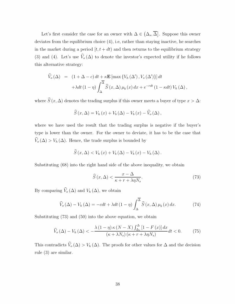
Let’s first consider the case for an owner with ∆ ∈(∆s,∆

]. Suppose this owner

deviates from the equilibrium choice (4), i.e, rather than staying inactive, he searches

in the market during a period [t, t+ dt) and then returns to the equilibrium strategy

(3) and (4). Let’s use Vo (∆) to denote the investor’s expected utility if he follows

this alternative strategy:

Vo (∆) = (1 + ∆− c) dt+ κE [max {Vh (∆′) , Vs (∆

′)}] dt

+λdt (1− η)

∫ ∆

∆

S (x,∆)µb (x) dx+ e−rdt (1− κdt) Vh (∆) ,

where S (x,∆) denotes the trading surplus if this owner meets a buyer of type x > ∆:

S (x,∆) = Vh (x) + Vb (∆)− Vb (x)− Vo (∆) ,

where we have used the result that the trading surplus is negative if the buyer’s

type is lower than the owner. For the owner to deviate, it has to be the case that

Vo (∆) > Vh (∆). Hence, the trade surplus is bounded by

S (x,∆) < Vh (x) + Vb (∆)− Vb (x)− Vh (∆) .

Substituting (68) into the right hand side of the above inequality, we obtain

S (x,∆) <x−∆

κ+ r + ληNs

. (73)

By comparing Vo (∆) and Vh (∆), we obtain

Vo (∆)− Vh (∆) = −cdt + λdt (1− η)

∫ ∆

∆

S (x,∆)µb (x) dx. (74)

Substituting (73) and (50) into the above equation, we obtain

Vo (∆)− Vh (∆) < −λ (1− η) κ (N −X)

∫ ∆

∆s[1− F (x)] dx

(κ + λNs) (κ+ r + ληNs)dt < 0. (75)

This contradicts Vo (∆) > Vh (∆). The proofs for other values for ∆ and the decision

rule (3) are similar.

38

References

Adrian, Tobias and Hyun Song Shin, 2010, The Changing Nature of Financial In-termediation and the Financial Crisis of 2007-09, Annual Review of Economics2, 603–618.

Afonso, Gara and Ricardo Lagos, 2014, An Empirical Study of Trade Dynamics inthe Fed Funds Market, working paper.

Afonso, Gara and Ricardo Lagos, 2015, Trade Dynamics in the Market for FederalFunds, Econometrica, forthcoming.

Atkeson, Andrew, Andrea Eisfeldt, and Pierre-Olivier Weill, 2014, Entry and Exitin OTC Derivatives Markets, working paper.

Babus, Ana and Peter Kondor, 2012, Trading and information diffusion in OTCmarkets, working paper.

Bao, Jack, Jun Pan, and Jiang Wang, 2011, The Illiquidity of Corporate Bonds,Journal of Finance 66, 911–946.

Duffie, Darrell, Nicolae Garleanu, and Lasse Pedersen, 2002, Securities Lending,Shorting and Pricing, Journal of Financial Economics, 66, 307–339.

Duffie, Darrell, Nicolae Garleanu, and Lasse Pedersen, 2005, Over-the-Counter Mar-kets, Econometrica, 73, 1815–1847.

Duffie, Darrell, Nicolae Garleanu, and Lasse Pedersen, 2007, Valuation in Over-the-Counter Markets, Review of Financial Studies, 66, 307–339.

Duffie, Darrell, Piotr Dworczak, and Haoxiang Zhu, 2014, Benchmarks in SearchMarkets, working paper.

Feldhutter, Peter, 2012, The same bond at different prices: Identifying search fric-tions and selling pressures, Review of Financial Studies 25, 1155–1206.

Gale, Douglas, 1987, Limit Theorems for Markets with Sequential Bargaining, Jour-nal of Economic Theory 43, 20–54.

Garleanu, Nicolae, 2009, Portfolio choice and pricing in illiquid markets, Journal ofEconomic Theory, 144, 532–564.

Gavazza, Alessandro, 2011, Leasing and secondary markets: Theory and evidencefrom commercial aircraft, Journal of Political Economy, 119, 325–377.

Glode, Vincent and Christian Opp, 2014, Adverse Selection and IntermediationChains, working paper.

Gofman, Michael, 2010, A network-based analysis of over-the-counter markets, work-ing paper.

39

Green, Richard, Burton Hollifield, and Norman Schurhoff, 2007, Financial Interme-diation and the Costs of Trading in an Opaque Market, Review of FinancialStudies 20, 275–314.

He, Zhiguo, and Konstantin Milbradt, 2013, Endogenous Liquidity and DefaultableDebt, Econometrica, forthcoming.

Hugonnier, Julien, Benjamin Lester, and Pierre-Olivier Weill, 2014, Heterogeneityin Decentralized Asset Markets, working paper.

Jankowitsch, Rainer, Amrut Nashikkar, and Marti Subrahmanyam, 2011, Price dis-persion in OTC markets: A new measure of liquidity, Journal of Banking andFinance 35, 343–357.

Kiyotaki, Nobuhiro and Randall Wright, 1993, A search-theoretic approach to mon-etary economics, American Economic Review, 83, 63–77.

Lagos, Ricardo, 2010, Asset Prices and Liquidity in an Exchange Economy, Journalof Monetary Economy, 57, 913–930.

Lagos Ricardo, and Guillaume Rocheteau, 2009, Liquidity in Asset Markets withSearch Frictions, Econometrica, 77, 403–426.

Lagos, Ricardo, Guillaume Rocheteau, and Pierre-Olivier Weill, 2011, Crises andLiquidity in OTC markets, Journal of Economic Theory, 146, 2169–2205.

Lagos, Ricardo and Randall Wright, 2005, A unified framework for monetary theoryand policy analysis, Journal of political Economy, 113, 463–484.

Lagos, Ricardo, and Shengxing Zhang, 2014, Monetary Exchange in Over-the-CounterMarkets: A Theory of Speculative Bubbles, the Fed Model, and Self-fulfillingLiquidity Crises, working paper.

Lester, Benjamin, Andrew Postlewaite, and Randall Wright, 2012, Information, liq-uidity, asset prices, and monetary policy, Review of Economic Studies, 79, 1209–1238.

Lester, Benjamin, Guillaume Rocheteau, and Pierre-Olivier Weill, 2014, Competingfor order flow in OTC markets, working paper.

Li, Dan and Norman Schurhoff, 2012, Dealer networks, working paper.

Li, Yiting, Guillaume Rocheteau, and Pierre-Olivier Weill, 2012, Liquidity and thethreat of fraudulent assets, Journal of Political Economy, 120, 815–846.

Malamud, Semyon and Marzena Rostek, 2012, Decentralized exchange, working pa-per.

Neklyudov, Artem, 2014, Bid-Ask Spreads and the Over-the-Counter InterdealerMarkets: Core and Peripheral Dealers, working paper.

40

Nosal, Ed, Yuet-Yee Wong, and Randall Wright, 2015, More on Middlemen: Equilib-rium Entry and Efficiency in Intermediated Markets, Journal of Money, Creditand Banking, forthcoming.

Pagnotta, Emiliano and Thomas Philippon, 2013, Competing on speed, workingpaper.

Roll, Richard, 1984, A simple implicit measure of the effective bid-ask spread in anefficient market, Journal of Finance 39, 1127–1139.

Rubinstein, Ariel and Asher Wolinsky, 1985, Equilibrium in a Market with Sequen-tial Bargaining, Econometrica 53, 1133–1150.

Shen, Ji, and Hongjun Yan, 2014, A Search Model of Aggregate Demand for Liq-uidity and Safety, working paper.

Taylor, John, 2001, Expectations, Open Market Operations, and Changes in theFederal Funds Rate, Federal Reserve Bank of St. Louis Review, 83, 33–47.

Trejos, Alberto and Randall Wright, 2014, Search-based models of money and fi-nance: An integrated approach, Journal of Economic Theory, forthcoming.

Vayanos, Dimitri, and Tan Wang, 2007, Search and Endogenous Concentration ofLiquidity in Asset Markets, Journal of Economic Theory, 66, 307–339.

Vayanos, Dimitri, and Pierre-Olivier Weill, 2008, A Search-Based Theory of theOn-the-run Phenomenon, Journal of Finance, 63, 1361–1398.

Vayanos, Dimitri, and Jean-Luc Vila, 2009, A Preferred-Habitat Model of the Term-Structure of Interest Rates, working paper.

Weill, Pierre-Olivier, 2007, Leaning Against the Wind, Review of Economic Studies,74, 1329–1354.

Weill, Pierre-Olivier, 2008, Liquidity Premia in Dynamic Bargaining Markets, Jour-nal of Economic Theory, 140, 66–96.

Wright, Randall and Yuet-Yee Wong, 2014, Buyers, Sellers and Middlemen: Varia-tions on Search-Theoretic Themes, International Economic Review 55, 375–397.

Zhu, Haoxiang, 2012, Finding a Good Price in Opaque Over-the-Counter Markets,Review of Financial Studies, 25 1255–1285.

41

Table 1: Model Predictions

This table summarizes the model predictions. The first column are the variablesthat we will measure empirically. The second column reports the variables in ourmodel, for which the variable in the first column is a proxy. The third column reportsthe predicted relation with the length of the intermediation chain L and the pricedispersion ratio DR. L is the ratio of the volume of transactions generated by dealersto that generated by customers, and is defined in (26). DR is the price dispersionamong inter-dealer trades divided by the price dispersion among all trades, and isdefined in (31). IG is a dummy variable, which is 1 if the bond is rated as investmentgrade, and 0 otherwise. Spread of a bond is the square root of the negative of thefirst-order autocovariance of changes in consecutive transaction prices of the bond.Maturity is the the time until maturity of a bond, measured in years. Turnover is thetotal trading volume of a bond in face value during the period, normalized by Size,which is the initial face value of the issuance size of the corporate bond, denominatedin million dollars. Age is the time since the issuance, denominated in years.

Variable Proxy for Relation with L and DR

IG c +Spread c +Maturity c −Turnover κ +Size X −Age X +

42

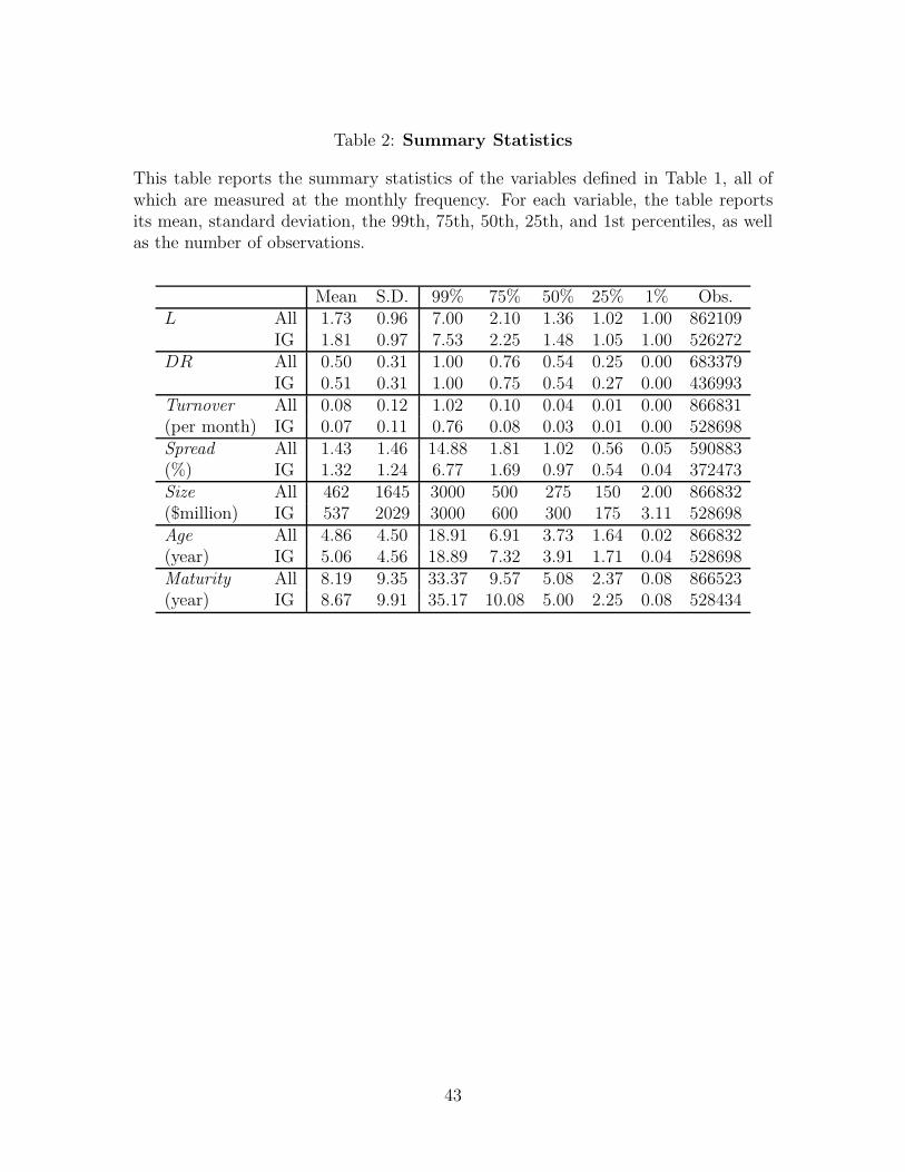
Table 2: Summary Statistics

This table reports the summary statistics of the variables defined in Table 1, all ofwhich are measured at the monthly frequency. For each variable, the table reportsits mean, standard deviation, the 99th, 75th, 50th, 25th, and 1st percentiles, as wellas the number of observations.

Mean S.D. 99% 75% 50% 25% 1% Obs.L All 1.73 0.96 7.00 2.10 1.36 1.02 1.00 862109

IG 1.81 0.97 7.53 2.25 1.48 1.05 1.00 526272DR All 0.50 0.31 1.00 0.76 0.54 0.25 0.00 683379

IG 0.51 0.31 1.00 0.75 0.54 0.27 0.00 436993Turnover All 0.08 0.12 1.02 0.10 0.04 0.01 0.00 866831(per month) IG 0.07 0.11 0.76 0.08 0.03 0.01 0.00 528698Spread All 1.43 1.46 14.88 1.81 1.02 0.56 0.05 590883(%) IG 1.32 1.24 6.77 1.69 0.97 0.54 0.04 372473Size All 462 1645 3000 500 275 150 2.00 866832($million) IG 537 2029 3000 600 300 175 3.11 528698Age All 4.86 4.50 18.91 6.91 3.73 1.64 0.02 866832(year) IG 5.06 4.56 18.89 7.32 3.91 1.71 0.04 528698Maturity All 8.19 9.35 33.37 9.57 5.08 2.37 0.08 866523(year) IG 8.67 9.91 35.17 10.08 5.00 2.25 0.08 528434

43

Table 3: Regression Results

This table reports the estimated coefficients from Fama-MacBeth regressions of inter-mediation chain length L and price dispersion ratio DR on a number of independentvariables, at monthly and quarterly frequencies. All variables are defined in Table1. T -statistics are reported in parentheses. The superscripts ∗, ∗∗, ∗ ∗ ∗ indicatesignificance levels of 10%, 5%, and 1%, respectively.

L DR

Monthly Quarterly Monthly QuarterlyIG 0.245∗∗∗ 0.239∗∗∗ 0.007∗∗∗ 0.004

(32.17) (20.43) (2.62) (1.14)Spread 0.073∗∗∗ 0.049∗∗∗ 0.004∗∗∗ 0.003∗∗

(17.17) (8.22) (4.47) (2.54)Turnover 0.199∗∗∗ 0.118∗∗∗ 0.217∗∗∗ 0.107∗∗∗

(11.48) (10.47) (26.58) (15.59)Size(×10−3) −0.012∗∗∗ −0.008∗ 0.021∗∗∗ 0.016∗∗∗

(3.73) (1.66) (15.17) (8.88)Age 0.025∗∗∗ 0.019∗∗∗ 0.001∗∗∗ 0.002∗∗∗

(23.92) (13.92) (5.39) (5.47)Maturity −0.001∗∗∗ 0.000 −0.001∗∗∗ 0.000

(3.72) (0.08) (6.00) (0.40)Const. 1.383∗∗∗ 1.311∗∗∗ 0.490∗∗∗ 0.573∗∗∗

(163.14) (136.07) (69.71) (50.47)

44

Figure 1: The evolution of demographics.

Panel A: The case without intermediation: ∆b ≥ ∆s

Panel B: The case with intermediation: ∆b < ∆s

45