financial liberalisation, bank excess liquidity and...

Glasgow Theses Service http://theses.gla.ac.uk/

[email protected]

Islam, Qamarullah Bin Tariq (2016) Financial liberalisation, bank excess liquidity and lending: A bank-level study for the economy of Bangladesh. PhD thesis. http://theses.gla.ac.uk/7271/ Copyright and moral rights for this thesis are retained by the author A copy can be downloaded for personal non-commercial research or study This thesis cannot be reproduced or quoted extensively from without first obtaining permission in writing from the Author The content must not be changed in any way or sold commercially in any format or medium without the formal permission of the Author When referring to this work, full bibliographic details including the author, title, awarding institution and date of the thesis must be given

http://theses.gla.ac.uk/

http://theses.gla.ac.uk/7271/

FINANCIAL LIBERALISATION, BANK EXCESS LIQUIDITY AND LENDING:

A BANK-LEVEL STUDY FOR THE ECONOMY OF BANGLADESH

Qamarullah Bin Tariq Islam

Submitted in fulfillment of the requirements for the Degree of Doctor of Philosophy in Economics

Adam Smith Business School College of Social Science

University of Glasgow

Glasgow December 2015

2

Abstract One of the main aims of financial liberalisation was to increase banking sector competition. Different policies were prescribed for this with one of the ultimate objectives being that banks would be able to lend without any constraint. If banks are able to lend their deposits fully then there will be no excess liquidity in the banking sector; even a significant increase of lending will imply reduction in excess liquidity. However, it is observed that although the process of financial liberalisation started around the early 1990s for most of the developing economies, still there is substantial excess liquidity problem in the banking sector in these countries, including Bangladesh. This study examined the possible reasons for excess liquidity and lending in Bangladesh using bank-level data of 37 banks for the period of 1997-2011 applying panel estimation methods. The first empirical chapter analysed how financial liberalisation affected the excess liquidity situation in banks. The second chapter examined how excess liquidity was related with business cycle and the recent financial crisis. The final empirical chapter looked at how financial liberalisation was related to lending. One key contribution of this study is that it applied an index of financial liberalisation to identify the process and its effect more comprehensively. Another important contribution of this research is to see if there were any definite patterns for different bank typologies. To address this, four bank-specific characteristics of ownership, size, mode of operation and age were used. Financial liberalisation was found to have significant positive relationship with excess liquidity as well as for lending for all types of banks. It was also observed that business cycle had a significant positive impact on excess liquidity. However less significant relationship between the financial crisis and excess liquidity showed the resilience of the banking sector in Bangladesh during the crisis. When bank-specific characteristics were analysed, the results showed that public banks had higher growth of excess liquidity and lower lending than private banks and new banks had lower growth of excess liquidity and higher lending than old banks. No definite differences could be observed between Islamic and conventional banks. It was also observed that public banks acted less procyclically than the private banks while large and new banks acted more procyclically than their counterparts. For the recent financial crisis, it is concluded that large and new banks had more excess liquidity than their counterparts while other typologies were found to be indifferent. Analysis of significant positive impact of financial liberalisation on both lending and excess liquidity suggested that prudent lending by banks to avoid loan default in the face of increased risk was a key for this parallel movement. Differences in interest rate according to bank-specific characteristics are found to be influential for the significant variations according to bank typologies.

3

Table of Contents Abstract 2

Table of Contents 3

List of Tables 9

List of Figures 11

Dedication 13

Acknowledgements 14

Declaration 15

List of Abbreviations 16

1 BACKGROUND AND JUSTIFICATION FOR THE STUDY 18

1.1 Introduction 18

1.2 Motivation for this Study 19

1.2.1 Different Strands of Studies 20

1.2.2

Alternative Possible Scenarios of the Impacts of

Financial Liberalisation 21

1.2.3 Excess Liquidity and Lending 23

1.2.4 Practical Experiences of Excess Liquidity in

Different Countries 26

1.3 Empirical Chapters of the Thesis 28

1.3.1 Financial Liberalisation and Excess Liquidity 28

1.3.2 Business Cycle, the Financial Crisis and Excess

Liquidity 29

1.3.3 Financial Liberalisation and Lending 30

1.4 Data Sources 31

1.5 Methodology 32

1.6 Structure of the Study 32

4

2 THE BANKING SECTOR IN BANGLADESH, EXCESS

LIQUIDITY AND LENDING 34

2.1 An Introduction of the Banking Sector in Bangladesh 34

2.1.1 Different Stages of the Banking Sector 34

2.1.2 The Financial System in Bangladesh 36

2.1.3 The Scheduled Banks in Bangladesh 37

2.1.4 Growth of the Banking Sector in Bangladesh 39

2.2 Excess Liquidity in Bangladesh: Some Stylised Facts 44

2.2.1 Excess Liquidity Situation According to

Traditional Classification of Banks 48

2.3 Credit in Bangladesh: Some Stylised Facts 50

2.3.1 Domestic Credit at Public and Private Sectors 50

2.3.2 Bank Advances by Economic Purposes 51

2.3.3 Ratio of NPL to Total Loans by Different Types

of Banks 53

Appendix 2.1 Generation of PCBs in Bangladesh 54

Appendix 2.2 Banking structure in Bangladesh 55

3 LITERATURE SURVEY 56

3.1 Introduction 56

3.2 Determinants of Excess Liquidity 58

3.3 Determinants of Lending 67

3.4 Methodology 72

Appendix 3.1 Some key estimated equations 76

Appendix 3.2 Summative table of some of the key findings 81

4 RELATIONSHIP BETWEEN FINANCIAL LIBERALISATION AND

EXCESS LIQUIDITY AT BANK-LEVEL 84

4.1 Introduction 84

5

4.2 Motivation of this Chapter 85

4.2.1 How Financial Liberalisation Can Reduce the

Problem of Excess Liquidity 85

4.2.2 Why Financial Liberalisation May Not Reduce the

Problem of Excess Liquidity and Rather Increase

It 86

4.2.3 Stages and Sequencing of Financial

Liberalisation 87

4.2.4 Importance of Bank-level Study 87

4.2.5 Contribution of this Chapter 90

4.3 The Empirical Approach 91

4.3.1 Dependent Variable 91

4.3.2 Explanatory Variables 91

4.3.2.1 Standard Control Variables 92

4.3.2.2 Key Variables of Interest 95

4.3.3 Variations According to Bank-specific

Characteristics 102

4.3.3.1 Variations According to Graphs 103

4.3.3.2 Statistical Tests for Difference among

Bank Typologies 105

4.4 Methodology 108

4.5 Sources of Data 114

4.6 Empirical Results 115

4.6.1 Data 115

4.6.2 Discussion of Results 116

4.6.3 Explanation of Results 121

4.6.3.1 Prudent Lending 122

6

4.6.3.2 Spread between Government Bill and

Interest Rate 123

4.6.3.3 Differences in Interest Rate 124

4.7 Conclusion and Policy Implications 127

Appendix 4.1 Data availability of banks in Bankscope 130

Appendix 4.2 Variable definitions 131

Appendix 4.3 Bank size classifications 132

Appendix 4.4 Generation of PCBs in Bangladesh 133

Appendix 4.5 Coding rules for the financial liberalisation

index 134

Appendix 4.6 Coverage area of this study of the banking

sector 140

5 EXCESS LIQUIDITY ACCORDING TO BANK TYPOLOGY,

BUSINESS CYCLE AND THE FINANCIAL CRISIS 142

5.1 Introduction 142

5.1.1 Capitalisation and Excess Liquidity 143

5.1.2 Structural and Cyclical Factors 144

5.1.3 Contribution of this Chapter 145

5.2 Previous Works 147

5.3 The Financial Crisis and the Bangladesh Economy 150

5.4 Empirical Approach 151



5.4.2.1 Standard Control Variables from Earlier

Studies on Lending and Excess Liquidity 153

5.4.2.2 Key Variables of Interest 156

5.5 Methodology 163

7

5.5.1 The Model 165

5.6 Empirical Results and Discussion 167

5.6.1 Empirical Results 167

5.6.2 Discussion of Results 175

5.7 Conclusion 179


6 BANK LENDING AND FINANCIAL LIBERALISATION: IS

THERE ANY DEFINITE PATTERN FOR DIFFERENT BANK

TYPOLOGIES? 182


6.2 Bank Typology 186

6.3 Contribution of this Chapter 193

6.4 Statistical Tests for Difference among Bank Typologies 195

6.5 Methodology 196

6.6 Data 197



6.6.3 Sources of Data 199

6.7 Empirical Results 200

6.7.1 Empirical Estimates 201

6.7.2 Robustness Checks 207

6.8 Conclusion and Policy Implications 209

6.8.1 Conclusion 209

6.8.2 Policy Implications 210


Appendix 6.2 Data availability 214

8

Appendix 6.3 Additional estimates 215

Appendix 6.4 Relationship between excess liquidity and

lending 216

7 CONCLUSION 218


7.2 Contribution to Literature and Summary Findings 219

7.3 Policy Recommendations 223

7.4 Concluding Remarks 225

BIBLIOGRAPHY 228

9

LIST OF TABLES

Sl. No. Name of Table Page

No.

Table 2.1 Excess liquidity according to different types of

banks (in per cent)

49

Table 4.1 Nominal EL, real EL and EL-SLR ratio in Bangladesh 85

Table 4.2 Bank classifications 99

Table 4.3 Wilcoxon rank-sum test results for bank typologies

of ownership, size, mode of operation and age

107

Table 4.4 t-test results for excess liquidity according to

ownership, size, mode of operation and age

108

Table 4.5 Correlation matrix of excess liquidity and the

dependent variables

116

Table 4.6 EL estimates applying two-step system GMM 117

Table 4.7 EL estimates applying two-step system GMM with

bank typologies

119

Table 5.1 The Hausman test result 166

Table 5.2 Correlation matrix of EL, BC, FC and other variables

of interest

168

Table 5.3 EL estimates applying FE 169

Table 5.4 EL estimates applying FE with bank typologies 171

Table 5.5 EL estimates applying RE with bank typologies 174

Table 6.1 Wilcoxon rank-sum test results for bank typologies

of ownership, size, mode of operation and age

196

Table 6.2 t-test results for ownership, size, mode of operation

and age

196

Table 6.3 Summary statistics of main regression variables

(annual data of 1997-2011)

200

10

Sl. No. Name of Table Page No.

Table 6.4 Correlation matrix of total lending and explanatory

variables

201

Table 6.5 Gross loan estimates applying two-step system GMM 202

Table 6.6 Gross loan estimates for bank typologies using FE

method

208

11

LIST OF FIGURES

Sl. No. Name of Figure Page No.

Figure 2.1 Bank assets (in billion taka) 39

Figure 2.2 Bank asset as a ratio of total asset (in per cent) 40

Figure 2.3 Number of bank branches 41

Figure 2.4 Bank deposit as a ratio of total deposit (in per cent) 42

Figure 2.5 Bank lending as a ratio of GDP 42

Figure 2.6 EL in nominal and real term(in billion taka) 45

Figure 2.7 Excess liquidity as a ratio of required liquid assets

(SLR)

46

Figure 2.8 Excess liquidity according to different types of banks

(in per cent)

50

Figure 2.9 Total domestic credit (in billion taka) 51

Figure 2.10 Bank advances by economic purposes (in per cent) 52

Figure 2.11 Ratio of gross NPL to total loans by type of banks (in

per cent)

53

Figure 4.1 Excess liquidity according to ownership 103

Figure 4.2 Excess liquidity according to size 104

Figure 4.3 Excess liquidity according to mode of operation 104

Figure 4.4 Excess liquidity according to age 105

Figure 4.5 NPL as ratio of total loan 123

Figure 4.6 Lending rate and government bill rate spread 124

Figure 4.7 Interest rate according to ownership 125

Figure 4.8 Interest rate according to size 126

Figure 4.9 Interest rate according to mode of operation 126

12

Sl. No. Name of Figure Page No.

Figure 4.10 Interest rate according to age 127

Figure 5.1 Capitalisation according to ownership 177

Figure 5.2 Capitalisation according to age 177

Figure 5.3 Capitalisation according to mode of operation 178

Figure 5.4 Capitalisation according to size 179

Figure 6.1 Total and private credit as a ratio of GDP in

Bangladesh

185

Figure 6.2 Gross loan according to ownership 187

Figure 6.3 Gross loan according to size 189

Figure 6.4 Gross loan according to mode of operation 191

Figure 6.5 Gross loan according to age 192

Figure 6.6 Consumer loan according to ownership 205

Figure 6.7 Consumer loan according to age 207

13

Dedication

To

My Mother

Who left this world just two days before my submission on 9 September 2014

14

Acknowledgements

I am thankful to my supervisor, Dr. Alberto Paloni, for his thorough supervision. His advice regarding things to be included, possible sources of data and econometric estimation were all very helpful. His guidance, constructive criticism and careful reading of the thesis led to several improvements for which I remain grateful to him. I also thank my second supervisors Dr. Joseph Byrne and Dr. Marco Avarucci for their advice whenever I met them. Dr. Marco Avarucci’s suggestions regarding the econometric part of the thesis were very helpful. I am also very thankful to my internal examiner Dr. Celine Azemar and external examiner Professor John Struthers for their valuable and detailed suggestions which enriched my thesis. My special thanks go to the Commonwealth Scholarship Commission for sponsoring me. The scholarship was crucially important in completing this study. They were very helpful, prompt and cooperative in correspondence. I am also thankful to the University of Rajshahi for giving me the study leave to complete this study. I wish to thank the staff and student in Economics at the University of Glasgow, especially Ms. Jane Brittin, Ms. Christine Athorne, my officemates Dr. Tariq Majeed and Dr. Simone Tonin for their help and encouragement. I am grateful to my colleagues in Economics at the University of Rajshahi for all their support. It is difficult to mention all the friends, colleagues and well-wishers whom I met here in Glasgow. I am grateful to them all. My mother, Professor Sultana Samiya Begum, left us all just two days before my submission but her prayers along with memories of love and affection kept me going to submit this thesis on time. I dedicate this thesis to her. My father Professor Tariq Saiful Islam constantly gave his encouragement and moral support which was crucial for me in completing this study. He is the most influential and a very special person in my life and will always remain so. I am going to mention three very special persons in my life: my elder brother Professor Abdullah Shams Bin Tariq, sister Dr. Sultana Fatima Tariq and brother Nazmullah Bin Tariq for their encouragement and help. My special thanks go to my brother-in-law Hafizur Rahman Khan and sisters-in-law Rasheda Kaneta and Sanjida Islam for their encouragement. My nieces and nephews were a source of joy during this time. I would like to express my gratitude to my aunty Razia Akter Khanam and other relatives for their encouragement. I especially remember my Aunty Alia Begum, whom we lost during this study. I am especially thankful to my father-in-law Muhammad Mahtab Uddin and mother-in-law Mahfuja Khatun and to all my in-laws who were constantly in touch for their encouragement. My wife, Dr. Mst. Hadikatul Jannat Al Mahmuda, was instrumental in completing my PhD. She left her job to accompany me and was always by my side, which included difficult phases. She always remained positive and showed her faith in me to successfully complete this study. She also demonstrated extreme patience, encouragement and understanding. Most importantly, Allah the Exalted led me through this learning period towards successful completion, which often looked long and unending. Qamarullah Bin Tariq Islam December 17, 2015

15

Declaration

I declare that, except where explicit reference is made to the contribution

of others, this dissertation is the result of my own work and has not been

submitted for any other degree at the University of Glasgow or any other

institution.

Signature

Printed name Qamarullah Bin Tariq Islam

16

LIST OF ABBREVIATIONS 2SLS Two-Stage Least Squares AR(1) First-order autoregressive process AR(2) Second-order autoregressive process BASIC Bank of Small Industries and Commerce BB Bangladesh Bank BBS Bangladesh Bureau of Statistics BC Business Cycle BDBL Bangladesh Development Bank Limited BIDS Bangladesh Institute of Development Studies BIS Bank of International Settlement BK Baxter-King BRC Banking Restructuring Committee BSRS Bangladesh Shilpa Rin Sangstha BT Bank Typologies CAR Capital Adequacy Ratio CEE Central and East European CEEC Central and East European Countries CEMAC Communaute Economique et Monetaire de l’Afrique Centrale

(Central African Economic and Monetary Community) CF Christiano-Fitzgerald CPI Consumer Price Index CRR Cash Reserve Ratio DFI Development Financial Institution EL Excess Liquidity EU European Union FBCCI Federation of Bangladesh Chambers of Commerce and Industry FC Financial Crisis FCB Foreign Commercial Bank FE Fixed Effects FSRP Financial Sector Reform Programme FV Fair Value GDP Gross Domestic Product GLS Generalised Least Squares GMM Generalised Method of Moments HP Hodrick-Prescott ICB International Commercial Bank IFS International Finance Statistics IMF International Monetary Fund InM Institute of Microfinance IRS Interest Rate Spread L/C Letter of Credit LDCs Less-Developed Countries LSDV Least Square Dummy Variable MCD Months for Cyclical Dominance MDFA Multivariate Direct Filter Approach MDG Millennium Development Goal MFI Micro-Finance Institution ML Maximum Likelihood

17

MOF Ministry of Finance MWW Mann-Whitney-Wilcoxon NBER National Bureau of Economic Research NCB Nationalised Commercial Bank NPL Non-Performing Loans NRB Non Resident Bangladeshi OLS Ordinary Least Squares PAT Phase-Average Trend PCB Private Commercial Banks RAKUB Rajshahi Krishi Unnayan Bank RE Random Effects ROA Return on Assets ROE Return on Equity SCB State-Owned Commercial Bank SLR Statutory Liquidity Reserve UNCTAD United Nations Conference on Trade and Development VAR Vector Autoregressive WCF Working Capital Financing WDI World Development Indicator WG Within Group

18

CHAPTER 1 BACKGROUND AND JUSTIFICATION FOR THE STUDY

1.1 INTRODUCTION

The setting of financial prices by central banks, especially in developing

countries, was a fairly common practice in the 1950s and 1960s. The

soundness of this approach was challenged by Goldsmith (1969) in the late

1960s, and by McKinnon (1973) and Shaw (1973) in the early 1970s. They

ascribed the poor performance of investment and growth in developing

countries to interest rate ceilings, high reserve requirements and

quantitative restrictions in the credit allocation mechanism.

According to them, these restrictions were sources of ‘financial

repression’, the main symptoms of which were low savings, credit rationing

and low investment. They argued that financial repression would restrain

savings by deliberately maintaining interest rates below their natural level.

As a result, growth would remain below its potential even when investment

opportunities are abound (McKinnon, 1973; Shaw, 1973; Fry, 1989). In

summary, the low rates of savings and investment that characterised

developing economies are assumed to be the results of government

intervention in the financial sector.

They proposed the theory of financial liberalisation, also known as the

McKinnon-Shaw hypothesis, according to which investment and savings are

repressed by a combination of controlled and low interest rates,

insufficient competition, high reserve requirements and government

allocation of credit. So the countries needed to deregulate interest rates,

lower the reserve requirements, dismantle any credit allocation schemes

and privatise as well as liberalise bank licensing in order to increase

competition. The rise of interest rates would then increase the incentive to

save and the resulting higher financial savings would lead to an

augmentation of investment levels. The increase in interest rates should

also weed out less productive investment, thereby leading to an increase in

19

the quality of investment. Judicious private bankers, without the

constraints of credit controls, would allocate funds to the most productive

users. Furthermore, increased competition would lower the spread

between savings and loan rates, thereby increasing the efficiency of the

financial system.

Therefore, according to this, there would be a higher rate of savings, which

would generate more investment and stimulate economic growth, which in

turn would augment savings, thereby creating a virtuous circle. However,

the key is to ensure that interest rates are market-determined as well as

banks are privately owned and operated so that bankers can make

decisions without political constraints. Moreover, sufficient number of bank

licenses must be made available to enhance competition while avoiding too

much deposit insurance and its associated problems of moral hazard

(encouraging risky behaviour) and adverse selection (leading to poorly run

banks).

1.2 MOTIVATION FOR THIS STUDY

As mentioned above, one of the expected outcomes of financial

liberalisation is a reduction in the level of excess liquidity. However, even

a cursory glance at media reports on banking would tell one that often one

can find significant levels of excess liquidity to exist. This is disturbing,

particularly when it coexists with an unmet demand for loans.

Therefore, it is interesting to study the dynamics of excess liquidity. Why

does is exist? Has financial liberalisation been able to have any impact on

it? What are the effects of other factors? Which of them are significant?

What effect has the recent financial crisis had on excess liquidity in banks?

Similarly, what are the effects of business cycle etc.?

Furthermore, as it will be discussed in greater detail in the literature

survey, after periods of extensive cross-country studies, a new approach

that has been introduced, but yet to be applied in great detail is that of

bank-level studies. These allow a closer look at how different types of

20

banks respond to a variety of factors. No such study exists for Bangladesh,

and such studies are still to address the issue of excess liquidity. How do

different banks behave regarding excess liquidity? Do they show any

differences? What policy measures could be introduced to address the issue

and in that case what aspects of bank typology should policymakers take

into consideration?

1.2.1 Different Strands of Studies

Over the years from when the financial liberalisation hypothesis was first

proposed, hundreds of empirical studies have been done on this topic. The

nature of these studies evolved over time with initial studies focusing on

the effects of financial repression followed by studies that examined

possible impacts of financial liberalisation while probable destabilising

implications of this process were analysed later on. A very eloquent

discussion on this can be found in the work of Gemech and Struthers

(2003).

The main strand of studies on the impact of financial liberalisation was

mainly done on its relationship with economic growth. From the early

1990s, empirical studies using large cross-section datasets with a particular

focus on the empirics of the finance–growth relationship started. A detailed

discussion of this cannot be presented here since it is not the aim of this

study but the following papers, among others, contain comprehensive

reviews on this aspect: King and Levine (1993), Hermes and Lensink (1996),

Arestis and Demetriades (1997), Levine (1997), Demirguc-Kunt and Levine

(2001), World Bank (2001), Green and Kirkpatrick (2002), Goodhart (2004),

Mavrotas and Son (2006) and Mavrotas (2008).

Another strand of literature on the effects of financial liberalisation

examined the follow-up link between financial liberalisation and poverty

reduction. Research on this area increased even more with the emergence

of the Millennium Development Goals (MDGs). Among others, the works of

Beck et al. (2004), Honohan (2004), Green et al. (2005) and Claessens and

Feijen (2006) shed important light on this area.

21

Researchers also started examining the impact of financial liberalisation

through different possible channels rather than looking at its direct impact

on economic growth and poverty. It was observed that financial

liberalisation works through increased savings with a positive correlation by

means of interest rate and thereby increasing investment to foster

economic growth (Levine, 1997). Although the conclusion in this regard is

still inconclusive1, there is a better consensus from the empirical studies on

the point that economic growth is positively related with moderately

positive real interest rate (Roubini and Sala-i-Martin, 1992; Bandiera et al.,

2000).

Institutional factors are also identified as one of the reasons for positively

helping the impact of financial liberalisation (Kayizzi-Mugerwa, 2003). It is

observed that good and well-functioning institutions are a key for

sustainable growth (Levine, 2003; Rodrik et al., 2004; Acemoglu et al.,

2005).

1.2.2 Alternative Possible Scenarios of the Impacts of Financial

Liberalisation

Financial liberalisation started in the late 1980s and in the early 1990s

around the world. The process of financial liberalisation is a multi-

dimensional and multi-faceted process, sometimes involving reversals

(Bandiera et al., 2000). Importance of country-specific studies was also

mentioned since they can be very useful tool to examine the effect of

financial liberalisation in depth (Guha-Khasnobis and Mavrotas, 2008).

One important area of the effect of financial liberalisation is bank lending.

From the discussion above, particularly in section 1.1, it can be observed

that one of the main aims of financial liberalisation was to increase the

banking sector competition. To attain this objective, countries will

deregulate interest rates, privatise and liberalise bank licensing, lower the

reserve requirements and dismantle any credit allocation schemes.

Moreover, astute private bankers, without the constraints of credit

1 See Fry, 1997, for a survey.

22

controls, will allocate funds to the most productive users. These two

together will mean that banks will be able to lend more. Banks’ ability to

supply more credit should imply that, keeping other things constant, there

will be significantly less or no excess liquidity in the banking sectors. In

other words, financial liberalisation should be able to sufficiently increase

lending to reduce or remove excess liquidity problem.

In this regard, possible effects of financial liberalisation can be classified

into various groups. One possible effect describes the positive impacts of

financial liberalisation on banking and how it can increase lending and

banking profitability. While the other scenario describes the probable

negative effect that financial liberalisation brings with it. Another

possibility states an in-between scenario where banks will be inclined to

lend more because of financial liberalisation but at the same time will take

into consideration the risks involved in it due to increased fragility

associated with the banking sector with this process. Therefore, banks will

only lend when they receive a minimum rate that will compensate risks and

other costs.

According to the first possibility, banking profitability increases in the short

run after the financial liberalisation. This is mainly due to the fact that

liberalisation includes the process of financial opening which ultimately

accumulates liquidity and thereby favours investment. Another reason for

increased profitability of the banking sector is attributed to reduced

control and supervision. This enables banks to lend in more risky projects

with higher returns.

The second possibility is that financial liberalisation can also lead to

banking fragility. The process of higher profit and return gradually involve

banks in lending to more risky projects, obviously with higher returns, but

also with probability of higher default. In addition, banks may also depend

on speculation when lending due to asymmetric information. Moreover,

there can be lack of proper institutional framework. All these together can

lead to deterioration of the financial situation of banks and lead to banking

23

fragility. This is evident from the experiences of both developed and

developing countries (Caprio and Kliengebiel, 1995; Lindgren et al., 1996).

This highlights the importance of analysing the benefits of liberalisation

carefully against the cost of the fragility and uncertainty that may come

along with this process. This has also led to the advocacy of some sort of

regulation in economies, particularly where the liberalisation is premature

(Caprio and Summers, 1993; Stiglitz, 1994).

Another alternative probability, proposed by Khemraj (2010), suggested

that in a relatively normal circumstance, there can still be excess liquidity

problem if banks decide to lend only when they receive a minimum interest

rate. This minimum rate should at least compensate the risks involved,

marginal transaction costs and the rate of return on a safe foreign asset. If

the borrower is unwilling or unable to take loan at this rate, then banks

will accumulate excess liquidity. On the other hand, banks can also

increase their lending rate to avoid risky loans. Thus, in the loan market,

loans and this non-remunerative excess liquidity can be perfect

substitutes2. It would be interesting to see which of these above possible

excess liquidity scenarios of the impact of financial liberalisation hold for

the banking sector in Bangladesh.

1.2.3 Excess Liquidity and Lending

Banks need to keep some part of their deposits as a reserve in the central

bank. In Bangladesh, this is called the cash reserve ratio (CRR). The

Bangladesh Bank (BB) which is the central bank of Bangladesh, has set a

percentage of demand and time liabilities which all banks need to keep

avoiding any sudden cash shortage. This is called statutory liquidity reserve

(SLR) which also includes the CRR. If banks hold more reserve than the SLR,

then it is said that banks have excess liquidity. The opportunity cost of

holding reserves at the central bank, where they earn very little or no

interest, increases the economic cost of funds above the recorded interest

expenses that banks tend to shift to its customers. In a study on CEMAC

2 This is observed to be reliable in an oligopolistic loan market following the industrial organisation banking model of Klein (1971) and Freixas and Rochet (1999).

24

(Communaute Economique et Monetaire de l’Afrique Centrale, which

represents Central African Economic and Monetary Community) countries,

Saxegaard (2006) observed that there are no remunerative alternatives for

excess liquidity.

Bank lending and excess liquidity are two very closely related aspects

(Alper et al., 2012) of the banking sector. Heeboll-Christensen (2011) used

the US data from 1987 to 2010 and found that “mechanisms of credit

growth and excess liquidity are found to be closely related.”

Given deposit, , the amount (1 − ) is available for

lending/investment. If the actual lending is , one may write:

= (1 − ) − (1.1)

Therefore generally it may be said that higher lending implies lower excess

liquidity. However, when one looks at how excess liquidity changes over

time with lending, one needs to take into account the fact that the deposit

is also changing over time. Thus taking differences:

∆ = ∆ (1 − ) − ∆ (1.2)

i.e. − = ( − )(1 − ) − ( − ) (1.3)

where, for simplicity it has been assumed that SLR does not change. It

should be obvious that if lending does not in(de)crease by the same

amount as the in(de)crease in deposit the excess liquidity will in(de)crease.

However, it is quite possible that lending increases but cannot keep pace

with the increase of deposit. In this case excess liquidity will also increase.

This is why empirical studies have found mixed relationships between

lending and excess liquidity.

Therefore, relationship between lending and deposit can lead to various

possible relationships between lending and excess liquidity. The

relationship is not so simple when deposit also increases. It will reverse

depending on whether growth in lending is larger or smaller than deposit

increase. There is difference of opinion about whether deposit is required

25

for lending. While the neoclassical view states that deposit is required for

lending, according to the post-Keynesian view, deposit is not a prerequisite

for lending. Assuming that all possibilities can occur, all the different

situations are discussed here. When lending increases more than deposit

increase (it can happen when deposit is not a prerequisite for lending or

when banks have liquid funds frm previous periods), then excess liquidity

will fall, implying negative relationship. But if increase in lending is less

than increase in deposit, then excess liquidity will rise (irrespective of

whether deposit is a prerequisite or not). Thus, among the two scenarios of

lending rise, the first scenario of (∆ ↑> ∆ ↑) will lead to a negative

relationship between lending and excess liquidity while the second scenario

(∆ ↑< ∆ ↑) will lead to a positive relationship between the two. The

third scenario of fall in lending will lead to increase in excess liquidity

(again irrespective of whether deposit is a prerequisite for it). For

Bangladesh, the second scenario is observed to be true where lending

increased less than deposit increase during the study period of 1997-2011.

For Fiji, Jayaraman and Choong (2012) found that excess liquidity and

lending were inversely related. The Bank of England also noted that the

available excess liquidity could be used to support lending (The Telegraph,

26 June 2013). Heider et al. (2009) described similar relationships but from

the alternative perspective as they concluded that illiquidity can reduce

the amount of lending. Saxegaard (2006) observed that excess liquidity in

the case of Sub-Saharan Africa could be due to deficient lending.

However, the above relationship where excess liquidity can act as an

increased amount of lending or vice versa is not always true. It has been

found that in Liberia, many banks have excess liquidity although there is

huge unmet demand for loans. Similar findings were also observed for

Bangladesh, where businessmen struggled to get loan but banks were

flooded with excess liquidity. Former President of the Federation of

Bangladesh Chambers of Commerce and Industry (FBCCI) Hossain

commented that though all the credit demand is not fulfilled, there is

26

excess liquidity. He stated, “Though the BB3 says there is no liquidity crisis,

as a borrower I face it” (The Daily Star, 21 June 2011). Similarly, Pontes

and Murta (2012) observed for Cape Verde that although there was excess

liquidity in the economy, still the lending rate was high, which should have

been low with high excess liquidity.

Of the above two paragraphs, the first one clearly shows how lending is

expected and generally observed to be inversely related with excess

liquidity while the second paragraph suggests that despite possibly being

related they may not always follow a certain pattern of negative

relationship. Hence, the aim of this work is to study excess liquidity and its

relationship with financial liberalisation at bank-level. Relationship of

excess liquidity with business cycle and the recent financial crisis will also

be seen. Finally, the relationship between lending and financial

liberalisation will be examined to have a better understanding of the

overall situation.

Normally one would expect any funds available to banks will be lent for

profit. However, as exemplified in the thesis, excess liquidity seems to be a

widely observed phenomenon even where the demand for lending is unmet.

Financial liberalisation, for example, would be considered a factor that

facilitates lending. Part of the motivation of this study is to understand the

banks’ behaviour regarding excess liquidity. What factors affect their

lending pattern and hence excess liquidity? How do they respond to policy

actions such as financial liberalisation, or other external factors such

financial crises, business cycles etc.? How do these responses vary across

the various types of banks that exist? These are some of the questions that

are addressed in this work (and again analysed in Section 7.2 of the

concluding chapter).

1.2.4 Practical Experiences of Excess Liquidity in Different Countries

Excess liquidity in Bangladesh is a constant phenomenon and frequently

mentioned by the central bank as well as by different businessmen and also

3 Bangladesh Bank, the central bank of Bangladesh.

27

reported in various newspapers. One senior official of the central bank

stated that, “banks in Bangladesh are flooded with excess liquidity”

(Reuters, Dhaka, 12 April 2009). This phenomenon is not only true overall,

but also true across banks. In the BB Annual Report (2009), it is written

that, “all the banks had excess liquidity.”

A detailed discussion of the excess liquidity situation in Bangladesh is

presented in Chapter 2 but it should be mentioned here thatBangladesh

experienced a dramatic rise in excess liquidity over the last 25 years both

in nominal and in real terms. Moreover, an increasing trend can be

observed even when it is expressed as a ratio of required liquid assets.

Excess liquidity is a problem not only in Bangladesh but also in many other

countries. Therefore, a detailed analysis of the situation in Bangladesh will

shed important light on the issues causing excess liquidity and how to deal

with it in Bangladesh as well as for other countries facing the similar

problem.

Researchers have found that excess liquidity is present in many countries.

For example, different studies on Africa and Caribbean countries have

observed persistent excess liquidity problem. Among others, Saxegaard

(2006) observed it for the CEMAC region, Nigeria and Uganda; Fielding and

Shortland (2005) found it for Egypt; while Khemraj (2006) had similar

observations for the Caribbean country of Guyana.

Similarly, it is also observed for the Asian countries where Agenor et al.

(2004) found this existent in Thailand, Eggertsson and Ostry (2005) in

Japan, Zhang and Pang (2008) in China. For the South Asian countries,

Mohan (2006) observed it for India while Majumder (2007) along with

Bhattacharya and Khan (2009) found it for Bangladesh.

It is obvious from the studies above that excess liquidity still remains a

major problem for most, if not all, of the developing economies. The

situation is also observed in the developed countries (e.g. Eggertsson and

28

Ostry, 2005; observed it for Japan) but since this study is related to a

developing economy and also because of similarities of the fact that

financial liberalisation was carried out in these countries, the literature

discussed were mainly those that focused on developing economies.

1.3 EMPIRICAL CHAPTERS OF THE THESIS

There will be three empirical chapters in this thesis. The first chapter will

discuss the relationship between financial liberalisation and excess liquidity

while the second will examine how excess liquidity is related with business

cycle and the recent financial crisis. The link between lending and financial

liberalisation will be analysed in the final empirical chapter.

1.3.1 Financial Liberalisation and Excess Liquidity

Most of the studies on the excess liquidity problem were done on a specific

country (e.g. Agenor et al., 2004; Fielding and Shortland, 2005; Aikaeli,

2006; Chen, 2008; Khemraj, 2008; Zhang, 2009; Yang, 2010). Only a few

studies (Saxegaard, 2006; Khemraj, 2010) examined this problem at a

cross-country level. These cross-country level studies were generally done

on Africa. According to our knowledge, there has been no study on excess

liquidity carried out at bank-level. In this respect, a study at bank-level

specifically on an Asian country like Bangladesh can shed important light

for the persistent excess liquidity in this region. It can also help in giving

further insight on excess liquidity prevailing in similar developing countries.

Therefore, the first empirical chapter of this study will aim to see the

probable effect of the possible determinants used in earlier studies of

excess liquidity along with an attempt to examine some additional

concepts. This will enable to explain better the stubbornly high excess

liquidity in these countries even after the financial liberalisation took place

and the possible reasoning for this excessive liquidity. An index of financial

liberalisation will be applied which is crucial due to the fact that the

process of financial liberalisation is a multi-faceted process (Bandiera et

al., 2000). This will help in avoiding misleading results when a dummy

variable or only a single variable is used to represent this versatile process.

29

Various bank-typologies will be applied to see if there are any differences

in excess liquidity according to bank-specific characteristics of ownership,

size, mode of operation and age.Thus the main questions that will be

examined in this study are as follows: (i) what is/are the reason(s) for the

prevalent excess liquidity even after the financial liberalisation took place?

(ii) how is financial liberalisation related with the excess liquidity situation

for the economy of Bangladesh? (iii) is it only due to the usual and

traditional factors that are discussed in different previous studies or is

there any other factor(s) which is/are normally ignored in the studies of

excess liquidity or is it a combination of both of these factors? (iv) what is

the relationship between excess liquidity and financial liberalisation for

different bank typologies?

1.3.2 Business Cycle, the Financial Crisis and Excess Liquidity

There have been several studies on the lending behaviour with differences

in bank ownerships in terms of business cycle. It has been observed that

public banks have a different lending pattern than private banks over the

business cycle with the general trend of public banks behaving procyclically.

But sometimes they behave counter-cyclically while sometimes they are

also found to behave acyclically. However, there is a gap in the existing

literature of studies on how other bank-specific characteristics play a role

in lending. Moreover, there was no study according to our knowledge on

business cycle and excess liquidity. Based on the earlier discussion on

relationship between lending and excess liquidity, this study will analyse

the difference in bank excess liquidity related to business cycle using some

additional typologies of banking. This will include bank size (based on bank

assets), banking mode of operation (Islamic versus conventional banks) and

bank age (based on year of establishment) in addition to bank ownership

(public versus private banks).4

Another interesting and related topic which may also affect lending

behavior of banks is crisis time. Generally it is observed that public banks 4Another classification of ownership based on whether a bank is domestic or foreign. This is due to the inavailablity of data in Bankscope for foreign banks in Bangladesh. Bankscope authority was also contacted in this regard.

30

are less efficient than private banks in non-crisis times. Nevertheless,

during the recent financial crisis of 2008-09, public banks were found to

play a positive role for the economy by either acting counter-cyclically or

less procyclically than private banks.

The objective of the second empirical chapter (Chapter 5) will be to fill

these gaps in this strand of literature with the main contributions

including: (i) examining the relationship between business cycle and excess

liquidity using bank-level data; (ii) investigating if there were any

differences in the relationship between business cycle and excess liquidity

according to bank typologies; (iii) examining the relationship between the

financial crisis and excess liquidity using bank-level data; (iv) investigating

if there were any differences in the relationship of the financial crisis and

excess liquidity according to bank typologies.

1.3.3 Financial Liberalisation and Lending

In relation to lending, the following three aspects of financial liberalisation

can be identified: (i) it reduces credit constraints of households engaged in

smoothing consumption when income growth is expected; (ii) it reduces

deposits required of first-time buyers of housing; and (iii) it increases the

availability of collateral-backed loans for households which already possess

collateral.

Most of the earlier works on lending were at an aggregate level. This was

mainly due to the fact that data were not easily available at disaggregated

levels (Gattin-Turkalj et al., 2007). Lack of sufficiently long historical data

at sector level was another reason for the lack of these types of studies (De

Nederlandsche Bank, 2000). It is also suggested that with more data

availability, future area of research should focus on breakdown (Calza et

al., 2001).

The related works between financial liberalisation and lending can be

broadly divided into three categories. The first category of studies tried to

investigate the effect of the financial liberalisation on lending but they

31

were done at an aggregate level and not at bank-level (Boissey et al., 2005;

Egert et al., 2006). The second category of works used bank-level data to

see the effect of some other phenomenon on lending pattern. For instance,

Cull and Peria (2012) used bank-level data for some countries in Eastern

Europe and Latin America but their main aim was to see if the lending

changed along with the process of the financial crisis of 2008-09. The third

category of research used some classifications of banking to see how they

are related to changes in the monetary policy. For example, Lang and

Krznar (2004) used the bank characteristics of ownership, capitalisation,

liquidity and size typologies of the banks to see how they differ in their

reaction to changes in the monetary policy in Croatia.

The aim of this work is to fill some of the gaps in the existing literature of

the above categories of studies and conduct a comprehensive study on bank

lending across banks applying different bank-specific characteristics to see

how they affected the lending pattern of the banking sector. The process

of the financial liberalisation will also be included to examine its effect on

these relationships.

The main objectives of this chapter of the thesis will be as follows:

(i)examining the relationship between financial liberalisation and lending

using bank-level data; (ii) investigating if there were any differences in the

relationship between financial liberalisation and lending according to

different bank typologies of ownership, size, mode of operation and age.

1.4 DATA SOURCES

The study will use bank-level data of 37 banks for the period of 1997 to

2011. The main source of data in this study will be the Bankscope database

which has data at bank-level. Some additional sources of data will also be

used. These include various issues of the Bangladesh Bank Annual Report

(the annual publication of the central bank in Bangladesh) and the

Statistical Yearbook, published by the Bangladesh Bureau of Statistics (BBS).

Moreover, data from international sources will also be taken which include

the World Bank database of World Development Indicator (WDI), the

32

International Monetary Fund (IMF) database of International Finance

Statistics (IFS). Some data from other published sources will also be used.

1.5 METHODOLOGY

The methodological and analytical basis for this study will be drawn from

the empirical literature focusing on financial liberalisation, excess liquidity

and lending. Moreover, literature related to business cycle and financial

crisis will also be studied. Descriptive statistics and econometric

techniques will be used to derive the results in this study and panel

estimation methods will be applied for estimations. Graphs and tables will

be provided when necessary to illustrate data and results of this study.

1.6 STRUCTURE OF THE STUDY

This study is organised into seven chapters. Chapter One, which is this

chapter, provides introductory background and motivation for this study.

Chapter Two will give an overview of the banking sector in Bangladesh,

specifically highlighting excess liquidity and lending situations.

Chapter Three will make a review of the relevant literature. This will be

done in two parts. In the first part, literature on excess liquidity will be

provided and in the second part, the review will discuss the determinants

of lending studied in various earlier works. Both theoretical and empirical

studies will be taken into account. This is very important as this will

ultimately help to specify the standard control variables of this study.

The relationship between excess liquidity and financial liberalisation in

Bangladesh will be empirically examined in Chapter Four. This relationship

will be investigated applying the standard control variables from earlier

studies on excess liquidity. Moreover, some key variables of interest will

also be investigated along with the reasoning for them to be included in

this study. Due to the complex nature of financial liberalisation, an index

of financial liberalisation will be used to comprehensively see the impact of

this liberalisation process. As this study will be at bank-level, hence

different bank-specific characteristics of ownership, size, mode of

33

operation and age will be included to see if there is any bank-level

difference of excess liquidity according to these characteristics.

Chapter Five will examine if and how the bank-specific characteristics,

used in this study, differ in terms of business cycle. Moreover, the effect of

business cycle on excess liquidity will also be examined. Since the period of

this study covers the recent financial crisis, popularly known as the ‘Great

Recession’, this chapter will also examine if and how this crisis impacted

the excess liquidity situation in Bangladesh. Moreover, the diversity of this

relationship in terms of ownership, size, mode of operation and age will

also be examined.

In the final empirical chapter (Chapter Six), lending pattern of the banking

sector in Bangladesh will be investigated. Following a similar classification

from the earlier empirical chapters, the effect of financial liberalisation

will be seen on lending as well as if there were any significant variations

across bank-typologies in the banking sector in Bangladesh.

Chapter Seven will present the conclusions of the thesis. This will include

the summary findings of the three empirical chapters, some policy

recommendations and the concluding remarks.

34

CHAPTER 2 THE BANKING SECTOR IN BANGLADESH,

EXCESS LIQUIDITY AND LENDING

2.1 AN INTRODUCTION OF THE BANKING SECTOR IN BANGLADESH

Bangladesh got independence on 16 December 1971. Soon after the

independence, the government of Bangladesh established the central bank

of Bangladesh, named the Bangladesh Bank5. Moreover, the government

also nationalised all the domestic banks of that time6. The foreign banks

were also permitted to continue and thus the banking sector of Bangladesh

started its journey.

2.1.1 Different Stages of the Banking Sector

As mentioned above, the banking sector in Bangladesh began its journey

with two Acts immediately after independence in 1971. One was related

with the central bank while the other was related with the nationalisation

of the domestic banks. Foreign banks were also permitted to continue their

operation independently. The main reasonings for the nationalisation of all

banks at that time were:

a) Branch expansion for providing services to the rural people;

b) Mobilisation of domestic savings, specially rural savings more

effectively;

c) Providing credit to the priority sector such as agriculture, small scale

and cottage industries etc;

d) Ensuring balanced regional development and removal of control on

banks by few individuals.

Later in the 1980s, the government decided to start privatising the

commercial banking sector. As a result, there were some privatisations of

the existing commercial banks while some new private commercial banks

5According to the Bangladesh Bank Order, 1972 (P.O. No. 127 of 1972) with effect from 16 December 1971. 6By Presidential Order No. 26 titled Bangladesh Banks Nationalization Order, 1972.

35

were also established at that time. The first private commercial bank, The

Arab Bangladesh Bank, was established in 1981-82.

By the mid-1980s, the government made a committee named ‘Money,

Banking and Credit’ headed by the then finance minister. It started

implementing the financial liberalisation which was termed as the

‘Financial Sector Reform Programme (FSRP)’. This process involved many

steps that included classifying overdue loans, restructuring the state-owned

commercial banks (SCBs)7 and private commercial banks (PCBs) as well as

fixing the interest rates on deposits and advances (Task Force Report,

1991).

The objectives of these steps taken at that time were to increase market

oriented incentive for priority sector lending, removing gradually the

distortions in the interest rate structure with a view to improving the

allocation of resources, adopting appropriate monetary tools to control

inflation, establishing appropriate accounting policies and modes of

recapitalisation, improving debt recovery process and strengthening the

capital market. Along with these, they also brought together some manuals

for operation and guidance of reporting system which were: lending risk

analysis, financial spread sheet, performance planning system, large loan

reporting system and new loan ledger card.

When the FSRP was ending, the government formed another committee

named ‘Banking Restructuring Committee (BRC)’ which suggested some

further steps for improvement in the banking sector. These steps included

an aggressive institutional renewal programme for Bangladesh Bank,

fundamental reforms of SCBs, better internal governance both in SCBs and

PCBs, penalties for imprudent lending, compliance with capital standards,

hiring of auditors of valuation audits of SCBs, special recovery efforts,

formation of a Bank Supervision Committee, strengthening the legal

process and institution of expending recovery of debt.

7 This type of bank is also called NCBs (nationalised commercial banks). Hence, NCBs and SCBs are used interchangeably.

36

They also took the following steps to improve the situation of the banking

sector in Bangladesh:

a) The amendment of Bangladesh Bank Order, 1972, to give Bangladesh

Bank legal autonomy over its affairs;

b) Reforms of supervision system of Bangladesh Bank to bring back

financial discipline;

c) Reforms of Bangladesh Banks (Nationalization) Order, 1972, to give

autonomy to SCBs’ boards so that SCBs could run on commercial

consideration;

d) Deposit insurance scheme to protect depositors’ interest;

e) Amendments to Bank Company Act, 1991, to effectively handle

problem banks;

f) Precluding crony (insider) lending and ensuring credit discipline.

All these were done to attain two major goals. Firstly, to attain an

effective legal system, good management and an effective central bank,

which were the three pillars of banking. Secondly, to shift focus from the

peripheral aspects of privatisation to the core aspects of dominance of

market forces, competition among banks, financial discipline through broad

based legal as well as regulatory base and operational efficiency.

2.1.2 The Financial System in Bangladesh

Before discussing in detail about the financial system in Bangladesh, a brief

description of the central bank of Bangladesh (the Bangladesh Bank), is

provided here. After independence, the Bangladesh Bank was established in

1972. It had nine different branches around the country. Of them, two

were in the capital, two were in the Rajshahi division and the rest were in

the other five divisions.

The rest of the banking system in Bangladesh is broadly divided into two

broad categories: the scheduled banks and the non-scheduled banks. The

scheduled banks worked according to the Bank Company Act 1991

(amended in 2003). The non-scheduled banks cannot perform all the

37

functions of the scheduled banks and were set up for some specific

purposes.

2.1.3 The Scheduled Banks in Bangladesh

The scheduled banks in Bangladesh can be broadly divided into four

categories: the state-owned commercial banks, the development financial

institutions (DFIs), the private commercial banks and the foreign

commercial banks (FCBs). At the moment, there are 57 scheduled banks in

Bangladesh. Of these, there are 4 SCBs, 5 DFIs, 42 PCBs of which 6 are Non

Resident Bangladeshi (NRB) banks and 9 FCBs.

State-owned Commercial Banks: After independence, the government of

Bangladesh nationalised all the commercial banks, except the foreign

banks. As a result, there were 6 SCBs at that time. They were: Sonali Bank,

Rupali Bank, Agrani Bank, Janata Bank, Pubali Bank and Uttara Bank. When

the government decided to start privatisation in the banking sector in the

early 1980s, Pubali Bank and Uttara Bank were privatised in 1985. Then in

1986, the government transformed Rupali Bank as a public limited

company. In 2007, the government also made the remaining three banks,

Sonali Bank, Agrani Bank and Janata Bank, as public limited company. As a

result, currently there are 4 SCBs in Bangladesh, which are working as

public limited companies.

Development Financial Institutions: Like the commercial banks, two

existing specialised banks were also nationalised. They were Bangladesh

Krishi Bank and Bangladesh Shilpa Bank. The first one was established for

the agricultural sector and the second one was for the industrial sector.

These banks were also called specialised banks as they were established

with specific objectives to attain. As Rajshahi Division was very prominent

in agriculture but distantly located from the capital, the Bangladesh Krishi

Bank was divided into two parts in 1987 to facilitate the agricultural

activities in this region. As a result, the Rajshahi Krishi Unnayan Bank

(RAKUB) was established to look after and develop the agricultural

activities in the Rajshahi division while the Bangladesh Krishi Bank

38

monitored agriculture for other parts of the country. To look after and help

promote the need of small and medium scale enterprises, the Bank of Small

Industries and Commerce (BASIC) was established in 1988. Later on the

government made it a specialised bank in 1993 and took control of it. In

2010, the government merged the Bangladesh Shilpa Bank with the

Bangladesh Shilpa Rin Sangstha (BSRS) and renamed it as the Bangladesh

Development Bank Limited (BDBL).

Private Commercial Banks: The PCBs started their operation in the early

1980s as privatisation of the banking sector started through Nationalization

(Amendment) Ordinance 1977. The Arab Bangladesh Bank was the first

private commercial bank which was established in 1982. Soon after it,

quite a few banks were established in the 1980s. These were IFIC Bank

Limited, National Bank Limited, Islami Bank Limited, City Bank Limited,

United Commercial Bank Limited and ICB (International Commercial Bank)

Islami Bank Limited. Along with these, two of the nationalised banks,

Uttara Bank Limited and Pubali Bank Limited, were privatised in 1983. The

main aims were to stop the continuous loss of these public enterprises,

increasing competition, improving their efficiency as well as customer

service and thereby increasing the flow of credit to all sectors of the

economy.

In the second stage, some more private commercial banks were established

between 1990 and 2000. This was the period when different measures of

the financial liberalisation were taking place. During this period, a very

large number of banks, 18 to be precise, were established. These are also

called the ‘Second Generation Banks’.

In the third stage (after 2000), some more banks were established. These

are called the ‘Third Generation Banks’. These banks used more of modern

technologies like online banking, debit and credit cards and ATM

(automated teller machine) booths which was also followed by ‘Second

Generation’ and other banks (more detail on all these banks along with

year of their establishment are provided in the appendix). Recently, 10

39

more banks were established after a long interval. Of these, 6 were PCBs, 3

were NRBs and 1 was a specialised bank.

Foreign Commercial Banks: The foreign banks were always allowed to

operate in Bangladesh. Even when the government decided to nationalise

all the commercial banks, they only did it for the domestic banks. The

foreign banks were allowed to carry on their activities as independent

institutions. Currently there are 9 FCBs in Bangladesh. These are: City Bank

NA, HSBC, Standard Chartered Bank, Commercial Bank of Ceylon, State

Bank of India, Habib Bank Limited, National Bank of Pakistan, Woori Bank

and Bank Al-Falah.

2.1.4 Growth of the Banking Sector in Bangladesh

The banking sector in Bangladesh achieved a very steady and robust growth

over the years ranging from its increase in terms of assets to number of

branches and as well as in terms of amount of deposit and lending.

Recently, some new banks have been given permission to start their

operation for further growth of this sector and meet the increasing

demand.

Bank Asset: Banking sector in Bangladesh went through a very rapid growth

from various directions.

Figure 2.1: Bank assets (in billion taka)

Source: Bangladesh Bank Annual Report, various issues.

0

1000

2000

3000

4000

5000

6000

7000

8000

2001 2002 2003 2004 2005 2006 2007 2008 2009 2010 2011 2012

Bank asset

40

Total asset was 1280.31 billion taka in 2001. It then almost doubled and

reached 2406.7 billion taka in 2007. In the next 5 years, it almost tripled

and reached a mammoth 7030.7 billion taka.

On the basis of the traditional classification of banks (i.e. SCBs, DFIs, PCBs

and FCBs), a shift in the percentage of assets can be observed between the

SCBs and the PCBs while it remained much more stable for the FCBs. In

2002, the asset of the DFIs as a ratio of total assets was 11.47 while it was

6.8 for FCB. The highest ratio in 2002 was for the SCBs with 45.56 per cent.

The PCBs had a share of 36.16 per cent.

Figure 2.2: Bank asset as a ratio of total asset (in per cent)


Over the next ten years, PCBs achieved significant growth and their share

of assets rose from 36.16 per cent to 62.18 in 2012. The share of the FCBs

almost remained stagnant, marginally increasing from 6.28 to 6.80 per cent

in this period. Both the SCBs and the DFIs experienced significant decline

and reduced to almost half of their shares of 2002. The SCBs share fell to

26.06 from 45.56 while the share of DFIs reduced to 5.48 from 11.47 in

these ten years.

0

10

20

30

40

50

60

70

SCB DFI PCB FCB

2012

2002

41

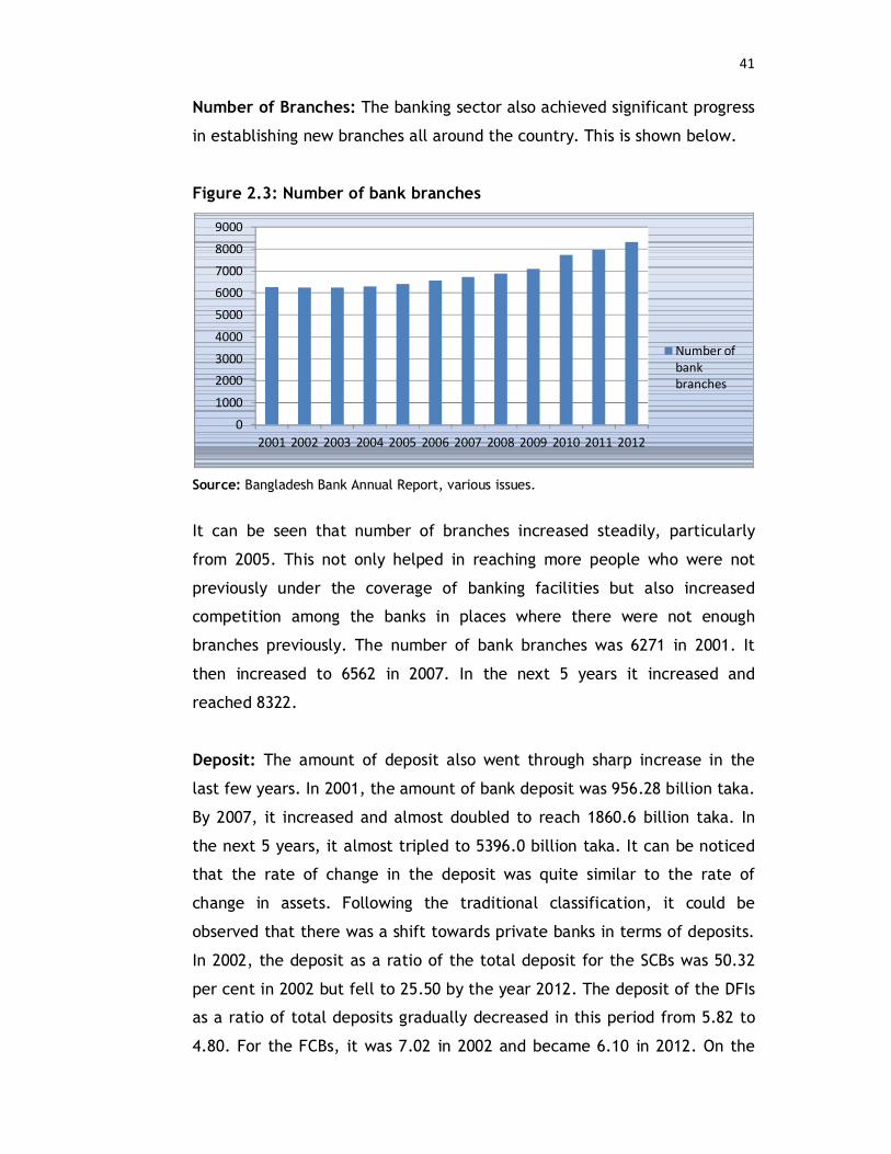
Number of Branches: The banking sector also achieved significant progress

in establishing new branches all around the country. This is shown below.

Figure 2.3: Number of bank branches


It can be seen that number of branches increased steadily, particularly

from 2005. This not only helped in reaching more people who were not

previously under the coverage of banking facilities but also increased

competition among the banks in places where there were not enough

branches previously. The number of bank branches was 6271 in 2001. It

then increased to 6562 in 2007. In the next 5 years it increased and

reached 8322.

Deposit: The amount of deposit also went through sharp increase in the

last few years. In 2001, the amount of bank deposit was 956.28 billion taka.

By 2007, it increased and almost doubled to reach 1860.6 billion taka. In

the next 5 years, it almost tripled to 5396.0 billion taka. It can be noticed

that the rate of change in the deposit was quite similar to the rate of

change in assets. Following the traditional classification, it could be

observed that there was a shift towards private banks in terms of deposits.

In 2002, the deposit as a ratio of the total deposit for the SCBs was 50.32

per cent in 2002 but fell to 25.50 by the year 2012. The deposit of the DFIs

as a ratio of total deposits gradually decreased in this period from 5.82 to

4.80. For the FCBs, it was 7.02 in 2002 and became 6.10 in 2012. On the

0

1000

20003000

4000

5000

60007000

8000

9000

2001 2002 2003 2004 2005 2006 2007 2008 2009 2010 2011 2012

Number of bank branches

42

contrary, the PCBs experienced significant growth rising from a share of

36.84 in 2002 to 63.60 per cent in 2012.

Figure 2.4: Bank deposit as a ratio of total deposit (in per cent)


Lending: Lending by banks, which was a key for increased investment, and

thereby growth, not only increased at gross level but it also rose as a ratio

of gross domestic product (GDP). This was estimated as domestic credit

provided by financial sector (% of GDP).

Figure 2.5: Bank lending as a ratio of GDP


0

10

20

30

40

50

60

70

SCBs DFIs PCBs FCBs

2002

2012

0

10

20

30

40

50

60

70

80

1997 2002 2007 2012

Lending-GDP ratio

43

This ratio was 29.94 per cent in 1997. In the next five years, it increased

dramatically to 50.44 per cent. The growth slowed down a bit but

continued and by the year 2007, it reached 58.21 per cent. This growth

picked up again in 2012 and became 68.98 per cent.

Recent Approvals for New Banks: There was a recent surge of approvals

for banks in Bangladesh. From 2012 onwards, 10 new banks were given

approval. This made the total number of banks reaching 57. The main aim

of these new approvals was aimed at strengthening the financial inclusion

of the unbanked people in the country. The previous time before this when

bank licenses was approved happened in 2000-01. Hence, expansion in this

sector was needed to address the current increased demand, particularly in

the face of the continuous economic growth that Bangladesh achieved over

the years as well as fulfilling the future banking requirements.

These new approvals were also required since population per branch was

21065 and the ratio of loan accounts per 1000 adults was only 42 (as of

2012). The situation was better in the neighbouring countries of India (with

a population of 14485 per branch and 124 loan accounts per 1000 adults)

and Pakistan (20340 and 47 respectively). Furthermore, a recent survey by

the Institute of Microfinance (InM) observed that only 45 per cent of the

surveyed people (based on nearly 9000 households) had access to banks and

micro-finance institutions (MFIs) for loans8.

The newly established banks consisted of one specialised bank and nine

commercial banks, of which six were PCBs and the remaining three were

NRB banks. A brief description about these new banks, established from

2012 onwards, is given below. However, they were not included in this

study due to their data unavailability for this study period.

Remittance was a major source of foreign exchange earnings and need

special attention. To address this, the Probashi Kallyan Bank, was 8 The central bank also took other measures to bring unbanked people under banking facilities. One of these initiatives was to provide banking account facility with a very nominal amount of deposit.

44

established to facilitate the financial transactions of the migrants. This

specialised bank is particularly related to remittance transfer, migration

and investment opportunities.

The newly established six PCBs were Union Bank Limited, Modhumoti Bank

Limited, Farmers Bank Limited, Meghna Bank Limited, Midland Bank

Limited and South Bangla Agriculture and Commerce Bank Limited while

the three new NRBs are NRB Commercial Bank Limited, NRB Bank Limited

and NRB Global Bank Limited.

It was made mandatory that these new banks would have to deposit 4

billion taka to the central bank of their paid-up capital before starting

their operation. Moreover, they need to maintain the 1:1 ratio when

opening branches in rural and urban areas. This was mainly to reach the

unbanked people who were mostly located in rural areas.

The NRBs will also need to deposit 4 billion taka to the central bank of

paid-up capital. Of these, 50 per cent will be from their sponsors while the

rest will be from the public offerings. Moreover, each shareholder must

hold at least shares worth 100 million taka while the maximum stake of

bank’s total paid-up capital for a shareholder can be 10 per cent.

2.2 EXCESS LIQUIDITY IN BANGLADESH: SOME STYLISED FACTS

Excess liquidity in Bangladesh was a constant phenomenon. This was

mentioned by the central bank, businessmen and was also reported in

newspapers. In the Bangladesh Bank Annual Report 2008-09, it was written

that, “Liquidity indicators measured as percentage (BB) of demand and

time liabilities (excluding inter-bank items) of the banks indicate that all

the banks had excess liquidity.”

When a bank holds reserves over and above the level sufficient to finance

its statutory required minimum reserves, deposit outflows and short-term

maturing obligations, it is reckoned as holding excess liquidity. The

opportunity cost of holding reserves at the central bank increases the

45

economic cost of funds above the recorded interest expenses that banks

tend to shift to customers.

If banks hold more reserve than the SLR, then it is said that banks have

excess liquidity. The data of nominal excess liquidity, real excess liquidity

and excess liquidity as a percentage of required liquid assets are given in

Figures 2.6 and 2.7. The real excess liquidity and excess liquidity as a

percentage of required liquid assets are given to have a real view of the

excess liquidity scenario in the economy.

It can be observed from Figure 2.6 that excess liquidity (EL) in nominal

terms did not change much around the late 1980s and early 1990s. Then it

experienced significant rise followed by a stable condition over the next

few years (particularly from 1994 to 1998). It then started to rise again and

continued with some exception (e.g. 2001, 2005 and 2006). It increased

dramatically in 2009 to reach an all time high.

Figure 2.6: EL in nominal and real term (in billion taka)

Source: Based on various issues of Bangladesh Bank Annual Reports and author’s own calculation.

The real excess liquidity of Bangladesh also saw a dramatic rise in the last

25 years. It was 18.71 billion taka in 1987. Then it fell over the next 3 years

before increasing again.

0.00

50.00

100.00

150.00

200.00

250.00

300.00

350.00

400.00

1987 1989 1991 1993 1995 1997 1999 2001 2003 2005 2007 2009 2011

EL in nominal term

EL in real term

46

It hovered around 20 billion taka till 1997. Then it increased till 2004 with

the exception of 2001. Though it fluctuated in the next few years but it

crossed the 100 billion mark in 2007 and reached a record high in 2009,

reaching a mammoth 267.09 billion taka. This came with a big jump in the

year 2009.

Even when excess liquidity data was given in real terms, it could be argued

that the rise in excess liquidity was due to increase in number of banks and

their branches leading to a rise in the total amount of deposit. To address

this, another figure is presented where excess liquidity is expressed as a

percentage of the required liquid assets, SLR.

It can be observed that changes in excess liquidity (as % of required liquid

assets) also followed an increasing pattern like nominal and real excess

liquidity though to a lesser extent. Although it went through fluctuations

but there was a growing trend in the long-run.

Figure 2.7: Excess liquidity as a ratio of required liquid assets (SLR)

Source: Based on various issues of Bangladesh Bank Annual Reports and author’s own calculation.

Excess liquidity as a percentage of the required liquid assets was 34.4 in

1987. It then fell in the next few years but then increased with some

fluctuations after 1991. From 1999, even with some fluctuation, the ratio

0.00

10.00

20.00

30.00

40.00

50.00

60.00

70.00

80.00

90.00

1987 1989 1991 1993 1995 1997 1999 2001 2003 2005 2007 2009 2011

EL as a % of SLR

47

substantially increased. It reached a huge 81.66 in 2009 which was also the

year when the amount of excess liquidity was all time high for Bangladesh.

But after 2009, it started falling again. Even after significant decrease in

the next two years, it was still quite high at 51.24 in June 2011.

The continuous rise of excess liquidity, as observed above, puts forward

the need for a study which can explain the reasons for it. This can be due

to factors that have been used in earlier studies of excess liquidity or can

be some other factors or it can be a combination of both. Nevertheless, it

is worth an effort to see why excess liquidity is so high and still increasing

in Bangladesh.

One point that needs to be noted is that excess liquidity fell before the

financial liberalisation programme (which was initiated in Bangladesh in

the early 1980s) but surprisingly it increased, with some exceptions, after

it. As mentioned before, the excess liquidity reached a record high of

267.09 billion taka (in real terms) in 2009.

Trying to explain the reason for this very high excess liquidity in 2009 it

was mentioned that “Bankers and experts attribute the build-up of the

excess liquidity in the banking system to poor investment situation, mainly

triggered by the on-going global meltdown” (The Financial Express, 5

August, 2009). A similar notion was mentioned in another newspaper,

“Economists and bankers think the investment flow is not picking up

because of the ongoing global recession” (The Daily Star, 13 July 2009).

According to former BB Chief Economist and currently Director General of

the Bangladesh Institute of Development Studies (BIDS) Mujeri:

“Credit to the private sector has declined in recent months due

mainly to lower import orders for capital machinery as well as

falling trend of major commodities prices in the global market”

(The Financial Express, 5 August 2009).

48

All possible reasons of this disproportionate excess liquidity in 2009 were

summarised very nicely by Bhattacharya and Khan (2009) in the following

words:

“The excess liquidity situation has been compounded by several

factors. Firstly, this fall in investment demand has been

exacerbated by import and export slowdown as a large share of

the bank credit in Bangladesh goes towards Letter of Credit

(L/C) opening. Further, fall in prices of majority of commodities

in the global market implies lower money demand for financing

imports. Secondly, because of the financial crisis the business

community has been prone to taking conservative steps with

regard to business decisions. This is evident through the decline

of L/C opening for capital machineries. Thirdly, credit

requirement of the government for financing of fiscal deficit has

also been moderate.”

2.2.1 Excess Liquidity Situation According to Traditional Classification of

Banks

With the recent establishment of 10 new banks, there are 57 scheduled

banks in Bangladesh. However, the description below is only for 47

scheduled banks as data for the new ones are not available for the period

under discussion. These 47 banks are generally divided into the following

four groups: nationalised, specialised, private and foreign.

The Islami banks maintain lower SLR instead of the existing one for the

conventional scheduled banks because of insufficient availability of Shariah

based approved securities. In other words, the Islami banks cannot

purchase treasury bills and bonds that involve receipt of interest, as the

Shariah rules ban payment or receipt of interest by any individual or

institution. The specialised banks (except BASIC Bank Limited) are

exempted from maintaining SLR fully because they were established for

specific objectives like agricultural or industrial development.

49

According to the Bangladesh Bank Annual Report of 2010-11:

“the commercial banks’ demand and time liabilities are at

present subject to a statutory liquidity requirement (SLR) of 19.0

percent inclusive of average 6.0 percent (at least 5.5 percent in

any day) cash reserve ratio (CRR) on bi-weekly basis. The CRR is

to be kept with the BB and the remainder as qualifying secured

assets under the SLR, either in cash or in Government securities.

SLR for the banks operating under the Islamic Shariah is 11.5

percent. The specialised banks (except Basic Bank Ltd.) are

exempted from maintaining the SLR. Liquidity indicators

measured as percentage of demand and time liabilities

(excluding inter-bank items).”

Excess liquidity situation for banks are given in the following table:

Table 2.1: Excess liquidity according to different types of banks (in per

cent)

Year NCBs DFIs PCBs FCBs 1997 2.7 9.7 6.0 11.2 1998 4.4 9.2 6.7 19.9 1999 5.2 8.7 8.0 31.4 2000 6.5 9.9 6.8 14.8 2001 5.7 8.9 6.2 14.3 2002 7.3 6.9 8.5 21.8 2003 8.4 5.8 9.8 21.9 2004 6.8 4.7 8.8 21.9 2005 2.0 6.2 5.1 23.6 2006 2.1 3.8 5.6 16.4 2007 6.9 5.6 6.4 11.2 2008 14.9 4.9 4.7 13.3 2009 17.6 7.1 5.3 21.8 2010 8.2 2.3 4.6 13.2

Source: Bangladesh Bank Annual Report, various issues. NCBs = Nationalised commercial banks, DFIs = State-owned development financial institutions, PCBs = Private commercial banks, FCBs = Foreign commercial banks.

For the nationalised commercial banks, the excess liquidity in per cent was

only 2.7 in 1997. With few exceptions, it gradually increased to 8.2 per

cent in 2010. It reached its peak of 17.6 per cent in 2009.

50

For the specialised banks, the situation was almost the opposite. It had 9.7

per cent excess liquidity in 1997 and then gradually decreased to 2.3 per

cent in 2010. In case of the private commercial banks, it could be seen that

excess liquidity hovered around 6 per cent for most of the years.

Figure 2.8: Excess liquidity according to different types of banks (in per

cent)

Source: Based on Table 2.1.

The scenario of excess liquidity in the foreign commercial banks had always

been different. It remained very high in relation to other types of banks

except in 2008 (when excess liquidity in NCBs were highest).

2.3 CREDIT IN BANGLADESH: SOME STYLISED FACTS

Credit in Bangladesh went through a very steady growth. It is worthwhile to

have a look at the lending pattern from different angles. Therefore, a brief

description is presented here both at aggregate and disaggregate levels.

Domestic bank credit is discussed first for total, public and private sector.

Then bank advances classified by major economic purpose are described.

2.3.1 Domestic Credit at Public and Private Sectors

Total domestic credit was 53.09 billion taka in 1997, increased to 101.40 in

the next five years, doubled to 204.27 in 2007 and rose to 433.53 in 2011.

0

5

10

15

20

25

30

35

1997 1998 1999 2000 2001 2002 2003 2004 2005 2006 2007 2008 2009 2010

NCBs

DFIs

PCBs

FCBs

51

Figure 2.9: Total domestic credit (in billion taka)


Gross credit to the private sector in 1997 was 38.95 billion taka, rose to

73.56 in 2002, more than doubled in the next five years reaching 150.77

and the growth continued reaching 340.71 by 2011. Credit to the public

sector followed a similar trend and reached 92.81 billion taka in 2011 from

14.14 in 1997. Of the credit to the public sector, net credit to government

increased sharply from 8.02 billion taka in 1997 to 73.44 in 2011 while

credit to other public sector rose from 6.12 in 1997 to 19.38 billion taka in

2011.

Total credit, credit to the private sector and credit to the public sector

increased by around eight-fold during this 15 year period with credit to the

private sector increasing slightly more than the public sector. However,

within the public sector, net credit to government increased by more than

nine-fold while credit to other public sector only tripled during this time.

2.3.2 Bank Advances by Economic Purposes

Trade was and still remains as the highest area of bank advances over the

years. It received 12.08 billion taka in 1997, which almost doubled in the

next five years. By 2007, it reached 48.62 billion and in 2011, it received

121.68 billion taka. The second highest area of bank advance was

manufacturing (excluding the working capital financing). It received 11.17

050

100150200250300350400450500

Total domestic credit in billion taka

52

billion taka in 1997, increased to 17.85 in 2002, almost doubled in the next

five years. By 2011, it reached 70.05 billion taka.

The third major area of bank advance in 1997 was agriculture (including

forestry and fisheries). It received 6.74 in 1997 which rose to 9.65 in 2002.

It remained stagnant in the next five years receiving 10.90 in 2007.

However, this sector experienced significant increase reaching 19.65 in

2011. Working capital for manufacturing was the fourth highest area of

receiving credit in 1997 (4.95). However, it rose dramatically over the

years and surpassed the advance received by agriculture (including forestry

and fisheries) in the next five years. The growth continued and reached

28.51 in 2007. By the year 2011, it received 47.06 billion taka.

Figure 2.10: Bank advances by economic purposes (in per cent)

Source: Bangladesh Bank Annual Report, various issues. Note: Manufacturing is estimated excluding working capital financing (WCF) which is given separately. Agriculture is estimated including forestry & fisheries.

It can be observed from the graph above that among the major sectors,

trade, working capital financing and others grew in terms of percentage

while agriculture and manufacturing (excluding WCF) fell. The growth in

the ‘others’ category can be mainly attributed to the growth in the

construction sector which was a mere 2.42 billion taka in 1997 but rose

rapidly to reach a significant amount of 24.19 in 2011, thus even surpassing

the advances made to the agricultural sector. Overall, this showed a

0

5

10

15

20

25

30

35

40

Trade Manufacturing Agriculture WCF Others

1997

2004

2011

53

structural shift away from agriculture. This is a noteworthy change for a

country where most of the people are still reliant on agriculture for

employment.

2.3.3 Ratio of NPL to Total Loans by Different Types of Banks

In Figure 2.11, the data for ratio of gross non-performing loans (NPL) to

total loans are provided. It showed the ratio for different types of banks.

Figure 2.11: Ratio of gross NPL to total loans by type of banks (in per

cent)

Source: Bangladesh Bank Annual Report, various issues. A similar trend of decrease can be observed for almost all types of banks

except the foreign ones which were very low in the beginning and it

remained so throughout. For the nationalised banks, it decreased from

36.60 per cent in 1997 to 15.70 in 2010.

For the DFIs, it fell from a huge 65.70 per cent to 24.20 during this period.

The decrease for the PCBs was the most dramatic as it fell by almost ten

times from 31.40 per cent in 1997 to only 3.20 per cent in 2010. As

mentioned before, it was always low for the foreign banks with the highest

of only 4.10 per cent in 1998.

0

10

20

30

40

50

60

70

80

1997 1998 1999 2000 2001 2002 2003 2004 2005 2006 2007 2008 2009 2010

NCBs

DFIs

PCBs

FCBs

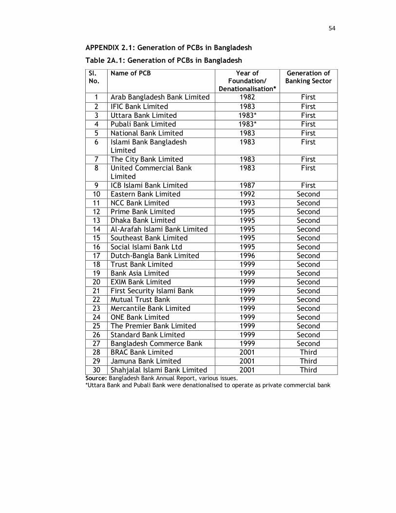
54

APPENDIX 2.1: Generation of PCBs in Bangladesh

Table 2A.1: Generation of PCBs in Bangladesh

Sl. No.

Name of PCB Year of Foundation/

Denationalisation*

Generation of Banking Sector

1 Arab Bangladesh Bank Limited 1982 First 2 IFIC Bank Limited 1983 First 3 Uttara Bank Limited 1983* First 4 Pubali Bank Limited 1983* First 5 National Bank Limited 1983 First 6 Islami Bank Bangladesh

Limited 1983 First

7 The City Bank Limited 1983 First 8 United Commercial Bank

Limited 1983 First

9 ICB Islami Bank Limited 1987 First 10 Eastern Bank Limited 1992 Second 11 NCC Bank Limited 1993 Second 12 Prime Bank Limited 1995 Second 13 Dhaka Bank Limited 1995 Second 14 Al-Arafah Islami Bank Limited 1995 Second 15 Southeast Bank Limited 1995 Second 16 Social Islami Bank Ltd 1995 Second 17 Dutch-Bangla Bank Limited 1996 Second 18 Trust Bank Limited 1999 Second 19 Bank Asia Limited 1999 Second 20 EXIM Bank Limited 1999 Second 21 First Security Islami Bank 1999 Second 22 Mutual Trust Bank 1999 Second 23 Mercantile Bank Limited 1999 Second 24 ONE Bank Limited 1999 Second 25 The Premier Bank Limited 1999 Second 26 Standard Bank Limited 1999 Second 27 Bangladesh Commerce Bank 1999 Second 28 BRAC Bank Limited 2001 Third 29 Jamuna Bank Limited 2001 Third 30 Shahjalal Islami Bank Limited 2001 Third

Source: Bangladesh Bank Annual Report, various issues. *Uttara Bank and Pubali Bank were denationalised to operate as private commercial bank

55

APPENDIX 2.2: Banking structure in Bangladesh

Table 2A.2: Banking structure in Bangladesh

Bank

Types

Number

of

Banks

Number

of

Branches

% of

Branches

Total

Assets

(Crore

Tk.)

% of

Industry

Assets

Deposits

(Crore

Tk.)

% of

Deposits

SCBs 4 3437 43.17 1629.2 27.8 1235.6 27.4

DFIs 4 1406 17.66 328.8 5.6 214.4 4.8

PCBs 30 3055 38.37 3524.2 60.0 2787.5 61.8

FCBs 9 63 0.79 385.4 6.6 272.2 6.0

Total 47 7961 100.00 5867.6 100.00 4509.7 100.00

Source: Bangladesh Bank Annual Report 2012-13.

56

CHAPTER 3 LITERATURE SURVEY

3.1 INTRODUCTION

In spite of efforts to liberalise and modernise financial institutions, markets

and instruments in less-developed countries (LDCs), the banking sector

remained the most important source of financing in these economies and it

is likely to remain so in the foreseeable future (Stiglitz, 1989; Singh, 1997).

Hence, the investment choice of banks could either contain role of finance

in growth or enhance that role. Thus, it was very important to analyse the

situation of excess liquidity in the banking system and also the reasons

behind it.

As discussed before, one of the main aims of financial liberalisation was to

increase the banking sector competition. For this, countries would

deregulate interest rates, privatise and liberalise bank licensing (in order

to increase competition), lower the reserve requirements and dismantle

any credit allocation schemes. Moreover, discerning private bankers,

without the constraints of credit controls, would allocate funds to the most

productive users.

Allocation of short- and long-term credit was also mentioned as one of the

channels between financial development and economic growth (Das and

Guha-Khasnobis, 2008; Yucel, 2009). These two together should mean that

banks would be able to lend more. It may be expected that ability of banks

to give more credit would imply that there would be less excess liquidity in

the banking sectors. In other words, financial liberalisation should reduce

the excess liquidity problem.

However, the practical experience of different developing economies

around the world told a different story. In many less developed countries

banks hold large quantities of excess liquidity in their asset portfolio, a

57

large part of which was non-remunerated (Fielding and Shortland, 2005;

Khemraj, 2006; Saxegard, 2006).

As described in Section 1.2.4, it was observed that various countries still

suffered from the problem of excess liquidity. For example, it was present

in the African countries (Fielding and Shortland, 2005; Gulde et al., 2006;

Khemraj, 2006; Saxegaard, 2006). Similarly, it was also observed that this

problem was present in China (Chen, 2008; Zhang, 2009; Yang, 2010) and

also in some other Asian countries (Agenor et al., 2004; Mohan, 2006;

Majumder, 2007; Zhang and Pang, 2008; Bhattacharya and Khan, 2009).

Holding huge amount of liquidity implied banks were trading off possible

profits with enormous risks related to existing vulnerable investment

avenues.

There was a difference of opinion among the economists on whether excess

liquidity was good for the economy or not. According to some economists,

excess liquidity was somewhat desired (Friedman and Schwartz, 1963;

Calomiris and Wilson, 1996; Ramos, 1996). This strand of argument

considered accumulation of excess reserves as protective liquidity. On the

other hand, some other economists viewed excess liquidity as an undesired

phenomenon attributed to exogenous economic factors (Bernanke, 1983,

1995; Ferderer and Zalewski, 1994).

There was also disagreement on whether excess liquidity was a demand or

a supply side phenomenon. If there was lack of credit demand from the

borrowers’ side, then it could be attributed to demand side. But if there

was enough demand for credit (in other words, if the credit demand was

not fulfilled) while the banks had excess liquidity, then it should be

attributed to the supply side.

Several authors had pointed to weak bank lending as one of the main

reasons for the build-up of excess liquidity. Wyplosz (2005) and Gilmour

(2005) identified weak bank lending, due to poor growth prospects, as the

reason for the increase in excess reserves in the Eurozone. Saxegaard

58

(2006), on the other hand, found that weak loan demand (owing to high

loan rates) accounted for the involuntary reserve accumulation in several

African countries.

However, in several other countries it was present side by side with

unfulfilled credit demand. For instance, it was found that banks in

Tanzania had excess liquidity though there was high private sector credit

demand (Aikaeli, 2011). This was supported by a World Bank study where

it was mentioned that “excess liquidity can coexist with very limited

investable funds” (Honohan and Beck, 2007).

This also seemed to be generally the case for Bangladesh. Though at times

of financial crisis, lowering of investment rates could contribute to excess

liquidity, generally excess liquidity existed alongside unment credit

demands. As already mentioned once, former President of the Federation

of Bangladesh Chambers of Commerce and Industry Hossain said, “Though

the BB (Bangladesh Bank) says there is no liquidity crisis, as a borrower I

face it” (The Daily Star, 21 June 2011).

All these imply that excess liquidity in many countries was not due to lack

of demand from the borrowers’ side but it was a situation arising from the

supply side. The banks were lending less than the amount they could or

were expected to lend due to some reasons other than the lack of demand.

So, in this study, the excess liquidity situation will be examined to explore

these possible factors.

The literature review section is broadly divided into two categories. The

first discusses the studies related to excess liquidity while the second part

describes the empirical works on lending.

3.2 DETERMINANTS OF EXCESS LIQUIDITY

Earlier studies on excess liquidity used various factors as the determinants

of excess liquidity. The most important explanatory variable of excess

liquidity that emerged from the previous studies was reserve requirement.

59

In their study on Thailand, Agenor et al. (2004) included it as one of the

independent variables and found it to be significant. Nyagetera (1997) also

agreed that reserve requirements play an important role in withdrawing or

enhancing liquidity in the banking system in Tanzania. In a separate

research, Aikaeli (2011) also studied excess liquidity problem for Tanzania

and found that along with other variables, the rate of required reserves

was also responsible for accumulation of excess liquidity in commercial

banks.

Chirwa and Michila (2004) mentioned that banks in many developing

countries were still subject to high liquidity reserve requirements even

after financial liberalisation. In sub-Saharan Africa, Seck and Nil (1993)

underscored the role of high reserve requirements, which acted as an

implicit financial tax by keeping interest rates high. While reserve

requirements may be designed with the aim of protecting depositors, the

availability of a pool of resources allowed for financing high fiscal deficits

through the implicit financial tax, thereby creating an environment that

could promote high inflation and persistent high intermediation margins.

The opportunity cost of holding reserves at the central bank, where they

generally would earn less interest than lending, increased the economic

cost of funds above the recorded interest expenses that banks tend to shift

to customers.

Other things being equal one would expect that an increase in lending rate

of the commercial banks would reduce lending and contribute towards

increasing excess reserves. This was observed in the study of Saxegaard

(2006) for sub-Saharan African countries. High lending interest rates,

whether caused by inefficiency or lack of competition, increased

borrower’s costs. By pricing the safer borrowers out of the market, high

interest rates could increase the risk of lending, making banks less willing

to lend and potentially resulting in credit rationing leading to high bank

liquidity. This was also mentioned in the work of Stiglitz and Weiss (1981).

60

Another important factor that was found to be related with excess liquidity

was deposit volatility. Agenor et al. (2004) found that deposit volatility

was one of the main factors that could explain the excess liquidity problem

for the economy of Thailand. Larsen (1951) also identified volatility as a

probable reason for excess liquidity. According to him, liquidity preference

of banks was affected by the formation of public expectations. To analyse

banks’ demand for liquidity, volatility of depositors’ cash preference

should thus be taken into consideration. Saxegaard (2006) observed that

currency withdrawal volatility9, which was very similar to deposit volatility,

could influence the excess liquidity situation.

Barajas et al. (2000) found evidence of a positive and significant

relationship between interest rate spread (IRS) and liquidity reserves in

the Colombian banking system. Brock and Rojas-Suarez (2000) and Saunders

and Schumacher (2000) observed that reserve requirement could have an

influence on the spread as they found evidence that suggested reserve

requirements acted as a tax on banks that translates into higher spreads in

a number of Latin American and developed countries.

Different authors observed that sometime banks kept excess reserve than

required in case of emergency. Mishkin (2001) explained that banks kept

excess reserves as an insurance against the costs associated with deposit

outflows. According to him, the higher the costs associated with deposits

outflow the more the excess reserves banks wanted to hold. This cost was

called the penalty rate and was generally proxied by either the discount

rate or the money market rate (Agenor et al. 2004; Aikaeli, 2006;

Saxegaard, 2006; Khemraj, 2010).

In a Bank of International Settlement (BIS) paper by McCauley and Zukunft

(2008) on the economy of Malaysia, the Philippines and Thailand, it was

observed that excess liquidity was due to weak credit growth in relation

9 Here the currency withdrawal volatility does not refer to ‘capital flight’ but is referring to volatility in the depositors’ behaviour in withdrawing their deposits from banks.

61

to domestic deposit growth. They measured this as a ratio of loan to

deposit.

One important factor that may cause excess liquidity and was used in some

of the earlier studies was excess savings. Chen (2008) considered five

indicators of excess liquidity on China. One of the determinants was excess

savings resulting from the poor social security network. This was supported

by some other studies where it was observed that one of the causes of

excess liquidity was the high saving ratio (Gu and Zhang, 2006; Wang, 2006;

McKinnon, 2006, 2007; Han and Chen, 2007; Roubini, 2007; Xia and Chen,

2007; Zheng and Yi, 2007). Jiao and Ma (2007), in their study of the excess

liquidity problem for the economy of China, used a slightly different

concept of savings where the variable they used was low consumption rate

paired with high savings rate.

Though Jiao and Ma (2007) studied the excess liquidity problem for the

economy of China using low consumption rate paired with high savings rate,

Qing (2006) used only the low consumption spending as an independent

variable to see its impact on excess liquidity in the economy. He observed

that low consumer spending resulted in large amounts of funds in the

banking system and thereby increased liquidity.

Two similar concepts of risks were used in different papers which were

very similar to each other. These were: the liquidity risk and the credit

risk. Agenor et al. (2004) used the concept of liquidity risk in their study

on Thailand while Aikaeli (2006) used credit risk as one of the variables

and found that credit risks were responsible for accumulation of excess

liquidity in commercial banks in Tanzania. Changes in the demand for cash

could be a proxy for this and the authors used the measure of deviation of

output from trend for it.

Many studies identified different external factors as reasons for excess

liquidity. Chen (2008), in a study on China, considered foreign exchange

system as one of the indicators of excess liquidity. This was supported by

62

some other studies where it was observed that one of the causes of excess

liquidity was the foreign currency exchange system (Gu and Zhang, 2006;

Wang, 2006; McKinnon, 2006, 2007; Han and Chen, 2007; Roubini, 2007; Xia

and Chen, 2007; Zheng and Yi, 2007). Khemraj (2006) identified several

possible determinants of excess liquidity. One of these was unsterilised

foreign exchange market interventions. He explained that sterilisation

involved simultaneously selling Treasury bills to mop up the liquidity

injected when the central bank buys foreign currencies from the foreign

exchange market. If there was total sterilisation then one could observe a

sterilisation coefficient of –1 while partial sterilisation was represented by

a coefficient value of between 0 and –1.

Bakani (2012), in his BIS paper, found that recent increase in foreign

exchange reserve was the main reason for excess liquidity in Papua New

Guinea. Jiao and Ma (2007) also observed that the continued growth of

foreign exchange reserve was one of the reasons for the excess liquidity

problem for the economy of China.

Another external factor used by authors was export. Jiao and Ma (2007)

used rapid rise in exports as one of the factors of excess liquidity and found

that it actually affected the excess liquidity. Similarly, Qing (2006)

observed that rapid growth of exports and investment could be a factor of

excess liquidity, especially if the consumption growth was way behind the

speed of investment and export.

Foreign aid was another external factor which was identified as a probable

factor leading to excess reserves. Gilmour (2005) argued that a significant

part of the increase in aid inflows in the early part of this century were

saved and channeled into excess reserves in Ethiopia. Saxegaard (2006) also

observed that excess liquidity could be due to variables such as foreign aid

which could account for the involuntary reserve accumulation in several

African countries.

63

Saxegaard (2006) mentioned that oil revenues could account for the

involuntary reserve accumulation. He found it to be true for some of the

African countries and this view was supported by one of the IMF (2005)

studies where they reported that in the case of Equatorial Guinea, large oil

inflows were associated with increase in excess liquidity.

Among other external factors, Bakani (2012) pointed towards the private

foreign direct investment as one of the reasons for excess liquidity in

Papua New Guinea while Khemraj (2006) identified remittance as one of

the possible determinants of excess liquidity as it could cause a build-up of

deposits (and reserves) as people convert foreign currency into local

currency.

There was also an indication in the literature that excess liquidity may vary

during periods of stress relative to normal situations, leading to greater

asset price volatility during the former and so disrupting liquidity targets

(Cohen and Shin, 2003). Morrison (1966) did a study on demand for excess

reserves in both panic and non-panic periods of banks. He concluded that

excess reserves were held as a buffer to avoid asset transaction costs

emanating from unforeseen transitory deposit shocks. This sort of excess

liquidity could also be interpreted as an insurance against deposit outflows.

Al-Hamidy (2013) found for the economy of Saudi Arabia that turbulent

international markets slowed down domestic credit growth and increased

excess liquidity.

Fielding and Shortland (2005) estimated a time-series model of excess

liquidity for the Egyptian banking sector and found that though financial

liberalisation and financial stability were found to have reduced excess

liquidity, these effects were offset by an increase in the number of violent

political incidents. They concluded that one of the reasons for excess

liquidity in Egypt was political instability.

Supply of credit or loan is expected to be related with excess liquidity

since an increase in the supply of credit from the banking sector should

64

mean that there would be less excess liquidity in the banking sector. Thus

excess liquidity could be taken as the other side of the coin of credit supply

and the factors that may affect the supply of credit could also be the

factors of excess liquidity. In this regard, the study of Andrianova et al.

(2010) could be helpful. They mentioned moral hazard (strategic loan

defaults) and adverse selection (lack of good projects) as two of the factors

that could affect the loan supply. Thus two very similar factors could be

used to explain the liquidity problem: one related to weak contract

enforcement and rule of law and the other related to weak and uncertain

economic growth. As both could lead to loan default, therefore impaired

loan was included in this analysis to see if these factors actually played any

role in the excess liquidity problem in Bangladesh.

Business cycle can have an effect on the excess liquidity situation of the

banks through its effect on lending. During economic boom, it was

expected that there will be an increase in demand for loans. Moreover, the

probability of loan default was expected to decrease during this time as a

result of borrowers doing well during this period. These will make banks

become softer in lending which may reduce the excess liquidity situation.

During the bust or economic downturn, banks would become stricter as the

probability of loan default increased. Moreover, investors also became

more careful in investing at this time and, and as a result, may end up

having higher amount of deposit in banks. Therefore, an inverse

relationship was expected to prevail between business cycle and excess

liquidity which meant that during the boom period of the business cycle,

there would be less excess liquidity while during the bust period, excess

liquidity will be more (Ruckes, 2004).

Although there were many works on business cycle and lending (particularly

using the bank ownership characteristics), but studies on the relationship

between business cycle and excess liquidity were very scarce. Most of the

studies on business cycle and lending were done at cross-country levels.

From these studies, it was generally observed that different types of banks

had different lending pattern over the business cycle.

65

Davydov (2013) observed that private banks’ lending pattern was generally

procyclical. The author observed that when public banks lending was also

procyclical, they were less procyclical than private banks in most cases. In

some cases, it was observed that lending of public banks could even be

counter-cyclical (Bertay et al., 2012). Some of the earlier studies found

mixed results for different countries or regions (Cull and Peria, 2012) while

some others did not find any significant difference in lending between

these two types of banks (Iannotta, et al., 2011). Thus it could be

concluded from these above mentioned works that the lending behaviour of

banks according to ownership was not same in all cases and varies where in

some cases they were procyclical, in some cases they were counter-cyclical

while in some cases they were acyclical.

This view of dissimilarity in lending according to ownership was also

supported by various country-level studies. For example, Berger et al.

(2008) observed it for Argentina, Lin and Zhang (2009) found this for China,

and Omran (2007) witnessed it for Egypt.

In some cases, it was observed that public banks and private banks were

almost equally efficient (Beck et al., 2005; Kraft et al., 2006). In another

study, Micco et al. (2007) observed that this feature of higher efficiency of

private banks was truer for developing countries than in the developed

countries. Davydov (2013) stated three possible reasons for the

comparative inefficiency of the public banks. They were: (i) political

interference, that deviate them from the profit maximisation aims; (ii)

incentives structure for managers were weaker than the private banks; and

(iii) inferior incentives for owners leading to poor monitoring.

However, it may be noted that the idea of comparing public and private

banks in terms of efficiency or profitability was rather misleading since

public banks had many other agenda along with the agendum of

profitability and hence pursuing solely the profit objective was not their

aim (UNCTAD, 2008). To attain these other objectives, the public banks

needed to compromise with the objective of profit maximisation to a

66

certain degree and became less profitable than their counterparts.

Therefore less profitability of public banks did not necessarily imply that

they were less efficient.

Another interesting and related topic which may also affect the lending

behaviour of banks was crisis time. The financial crisis and business cycle

could be closely related due to the fact that if the downturn or recession of

the business cycle goes on for a long time, it could lead to crisis. This

reasoning was supported by Bordo et al. (2001): “crises are an intrinsic part

of the business cycle and result from shocks to economic fundamentals.”

Similar to the difference in bank lending in terms of ownership during

business cycle, it was also observed that banks lend differently according

to ownership during crisis time. In different cross-country studies on non-

crisis times, it was commonly found that public banks were less efficient

and sometime led to lower financial development than private banks (Barth

et al., 2004; Bonin et al., 2005; Duprey, 2013).10

However, during the recent financial crisis of 2008-09, the public banks

played a positive role for the economy by generally acting counter-

cyclically (Allen et al., 2013) or less procyclically (Fungacova et al., 2013).

This was crucial and helped the economy to stabilise as the domestic

private banks acted procyclically (Kowalewski and Rybinski, 2011; Cull and

Peria, 2012). This was also true for earlier financial crises in Asia and Latin

America in the 1990s (Hawkins and Mihaljek, 2001).

Micco and Panizza (2006), in their study of 179 countries, mentioned four

possible reasons why public banks stabilised credit: (i) public banks do it as

part of their objectives, (ii) with possibilities of bank failures, people

generally considered public banks to be a safer place and hence these

banks end up having a better deposit base during the crisis which led them

to a better position for smoothing credit, (iii) public bank managers could

10In some cases, it was also observed that this feature of higher efficiency of private banks was truer for developing countries than the developed countries.

67

be lazy due to lack of having a proper set of incentives, (iv) in election

years, politicians could try to influence public bank lending.

Studies on financial crisis and excess liquidity could be broadly divided into

two categories. One group analysed how excess liquidity acted as one of

the factors for the financial crisis (Palma, 2009; Acharya and Naqvi, 2012;

Brana et al., 2012) while the other group discussed how financial crisis

could affect excess liquidity.

One of the possible effects of financial crisis was that it increased

uncertainty and riskiness in the economy. This made lending riskier for the

banks. Therefore, banks lent less and thereby the excess liquidity situation

increased. For example, Agenor et al. (2004) observed this for Thailand

while Ashcraft et al. (2011) found it for US. Montoro and Moreno (2011)

found similar results for Peru. In another study, Murta and Garcia (2010)

examined excess liquidity for banks in the Euro area.

The most direct empirical study till now, to our knowledge, that examined

the effect of the recent financial crisis on the excess liquidity situation of

banking sector was carried out by Pontes and Murta (2012). They studied

this relationship for the African economy of Cape Verde. Their results

suggested that the crisis decreased the excess liquidity in the economy.

The possible reasons included the extreme dependence of the economy on

the external economy (especially remittance) as well as the

underdevelopment of the financial markets.

3.3 DETERMINANTS OF LENDING

Different studies used different sets of explanatory variables. Some of

them were more common while others were used less frequently across

studies. The three most common explanatory variables used in the earlier

studies were: economic growth, interest rate and the lagged dependent

variable.11

11The definition of these variables and their measurement are given in detail in Appendix 6.1.

68

It was expected that if there was economic growth, there would be higher

demand for investment and also increased demand for loan. This was

mainly due to the fact of favourable economic conditions. Therefore,

economic growth should affect lending positively. This was also observed in

earlier empirical studies (Cottarelli et al., 2003; Kiss et al., 2006; Kraft,

2006; Gattin-Turkalj et al., 2007; Brissimis et al., 2014). To capture

economic growth, real GDP was used in this study.

The rate of interest was another variable that had been frequently used in

studies of lending. It was expected to have a negative relationship with

lending since lower interest rate should increase the demand for credit and

vice versa (Egert et al., 2006). In this study, to capture the effect of

interest rate, interest rate was taken in real terms, which was calculated

by deducting the current inflation from the nominal interest rate. This was

done to reflect the true effect. To convert interest rate into real terms,

both consumer price index (CPI) and GDP deflator were used.12

Lagged Dependent Variable was also applied in earlier studies. It was

found to have a positive effect on lending (e.g. Gattin-Turkalj et al., 2007).

Hence, this variable was included in this study to capture and account for

the persistence of lending from the earlier period.

Since financial liberalisation took place in most of the economies around

the 1990s, the impact of this process was part of some of the recent

studies on lending. As the liberalisation process was initiated at the

backdrop of the financial repression and was proposed to remove various

credit restrictions to ensure the free flow of credit, it was expected that

there will be a positive relationship between liberalisation and lending.

Different bank-specific characteristics could play a role in lending. These

include bank ownership, size, mode of operation and age.13 Summarily it

can be said that there could be differences in the lending behaviour of 12 Results using the real interest rate using CPI are presented in the main text while that using the other measure of real interest rate are given in Appendix 6.3. 13These characteristics are discussed in detail in Sections 4.3 and 6.2.

69

banks according to these characteristics and it would be interesting and

worthwhile to see if and how these characteristics significantly differed

lending of banks.

It was generally believed that the availability of bank lending depends, in

addition to the traditional factors, on the process of financial

liberalisation. With the process of liberalisation, banks would be able to

lend more due to the fact that entry into the banking sector would be

easier. Furthermore, the expansion of the banking sector would also

increase the credit supply and reduce the lending rate (Boissay et al.,

2005; de Haas and van Horen, 2010).

However, the process of liberalisation could also increase the interest rate

volatility and asset prices. This rise in asset and property prices could also

trigger a temporary unwarranted credit boom (Bandiera et al., 2000).

Furthermore, competition among banks could increase as a result of the

liberalisation process which may end up in a situation where banks lend

imprudently (Caprio et al., 2006). But imprudent lending could be due to

outright managerial failure also (Honohan, 1997). Therefore, the overall

impact of financial liberalisation on credit mainly leant towards the fact

that lending would increase. This positive relationship between

liberalisation and lending was also supported by earlier empirical works

(Cottarelli et al., 2003; Gattin-Turkalj et al., 2007)14.

Since it was a continuous and multi-faceted process (Bandiera et al., 2000),

the results could be misleading if a binary dummy variable was used to

represent this versatile process. Therefore, to address the process in a

more comprehensive way, an index of financial liberalisation was used by

Abiad et al. (2010). Although most studies either used a binary dummy or a

single indicator of liberalisation, the use of an index to appropriately

capture the process of liberalisation was not uncommon. For example,

14 Although many earlier studies observed that even with the financial liberalisation, credit for firms remained a major problem and this was true for many developing countries around the world. For a comprehensive survey, see the works of Aryeetey et al. (1997) and Nissanke (2001), among others.

70

Cottarelli et al. (2003) also applied a similar index in their study of CEEC

countries. In this study an index motivated by that of Abiad et al. (2010)

was used.

The earlier related works on lending could be broadly divided into three

categories. The first category of these studies investigated the effect of

financial liberalisation on lending. These were done at an aggregate level

and not across banks (Boissey et al., 2005; Egert et al., 2006).

The second category of research used some classifications of banking to see

how they were related to the changes in the monetary policy. For example,

Lang and Krznar (2004) used the bank characteristics of ownership,

capitalisation, liquidity and size to see how they differed in their reaction

to changes in the monetary policy in Croatia. But they did not see how the

process of financial liberalisation affected lending according to these

characteristics.

The third category of works, which was analogous to this study, used bank-

level data to see the effect of some other phenomena (than financial

liberalisation) on lending. For instance, Cull and Peria (2012) used bank-

level data for some countries in Eastern Europe and Latin America but their

main aim was to see if lending changed along with the process of the

financial crisis of 2008-09.

There were quite a few studies on European Countries. Among the recent

cross-country studies on lending, Brzoza-Brzezina (2005) studied the new

European Union (EU) countries and found that lending generally increased

across countries. However, the degree differed from country to country

with Hungary and Poland experiencing a very strong growth as well as

Ireland and Portugal. Similar observations of differing degree of changes

were observed by Egert et al. (2006) in their study of 11 Central and East

European (CEE) countries. They observed that while some countries

experienced steady growth (e.g. Estonia and Latvia), some others

experienced growth after initial slowdown (e.g. Hungary and Croatia) while

71

some others experienced almost steady decline (e.g. Czech Republic and

Bulgaria).

For example, Calza et al. (2001) studied the lending pattern of the Euro

area while Cottarelli et al. (2003) studied the Central and East European

Countries (CEEC). They observed that although lending as a ratio of GDP

increased in most of the countries (e.g. Bulgaria, Croatia, Poland and

Slovania) but it declined for some other countries (e.g. Czech Republic,

Slovak Republic and Macedonia). This sort of mixed findings was also

supported by, among others, Schadler et al. (2004) and Kiss et al. (2006). In

another work by IMF (2004) on some of the European countries, excessive

growth in credit was recognised. It was observed that Bulgaria, Romania

and Ukraine experienced very high credit growth. The paper observed that

although increase in lending was a good sign but excessive credit growth

could be a matter of concern.

In a study of 16 industrialised countries across regions, Hofmann (2001)

observed that credit as a ratio of GDP increased in most of the countries.

The author also observed that growth in credit and economic growth moved

very closely with each other, supporting procyclicality of financial

development. In another IMF (2004) study, it was observed that although

lending increased across countries and regions, it increased more in

Southeast Asian countries.

The analysis of the effect of the liberalisation process on lending pattern in

Bangladesh started almost immediately after the liberalisation process

started in this country. Khan (1993) observed that banks were not able to

allocate credit efficiently, mainly due to the problem of imperfect

information. However, he also pointed out that it “might be too early to

determine the benefit of the liberalisation.” In another study, Ahmed

(1995) observed mixed implications of the liberalisation on the banking

sector in Bangladesh. Khan et al. (2011) observed that lending in

Bangladesh increased for all the banks since the financial liberalisation

started. They examined lending by traditional categories of banking data as

72

was generally available in Bangladesh. According to this, the scheduled

banks were classified into SCBs, DFIs, PCBs and FCBs. They also analysed

lending according to sectors and found that loans were gradually moving

from agriculture towards industrial sector.

One important point to note was that almost all studies on Bangladesh

were either done at an aggregate level or when they were done at a

disaggregated level, the banks were classified into the earlier mentioned

categories of SCBs, DFI, PCBs and FCBs. This was done possibly because of

easier data availability as the data were available in this format. However,

these studies missed out the possible effects of different bank-specific

characteristics which may have an impact on the lending behaviour of

banks. Therefore, to investigate if these characteristics significantly (or

insignificantly) affected lending of banks, it was crucially important to

include these characteristics and study them accordingly. This was

attempted in this bank-level study for the banks in Bangladesh.

3.4 METHODOLOGY

In this section, some of the methodologies applied in earlier studies on

excess liquidity and lending are discussed. In the first part, the works on

excess liquidity are discussed followed by studies on lending in the second

part. Furthermore, some of the important equations in the earlier studies

on excess liquidity and lending are described in the appendix of this

chapter.

Various estimation methods were employed by different authors in their

works. Most of them used system GMM (generalised method of moments)

for its overall superiority over other panel estimators. However, different

other methods were also applied by some authors. The methods used in

these studies and their rationale are briefly described in the following

paragraphs.

When the country-specific studies were considered, it was found that

different methods were used in different studies. Lin et al. (2012) used the

73

GMM method for Japan in their study of lending and financial crisis.

According to them, the reason for using the Arrellano-Bond (1991) GMM

estimator was that it allowed for more flexibility in specifying which

variables were to be taken as endogenous or truly exogenous and to assign

appropriate instruments to endogenous variables. Moreover, the qualities

of all the designations could be tested by different standard tests and it

could be evaluated whether the variables of interest were independent of

the error term. The Arrellano-Bond (1991) method also enabled to take into

account the possible autocorrelation in the dependent variables.

Fungacova et al. (2013) used the maximum likelihood (ML) estimation

method to see the relationship between lending and financial crisis in

Russia for the stochastic frontier model. According to them, this method

helped in capturing the time dimensionality by estimating the model in a

series of pooled cross-sections, rather than a panel, because it was

important that all model parameters, including residual distributions, could

change over time.

To investigate if bank ownership exerted an impact on credit supply during

the financial crisis, they added dummy variables for state ownership and

foreign ownership to the frontier model as these variables were always

viewed relative to domestic private ownership. Further, they included

interaction between ownership and time dummy variables for each quarter

of the sample period. Moreover, they also stated that the respective

parameters of the time variable effects of state and foreign ownership

indicated the difference in the change of the proportionality factor of

state-controlled and foreign banks relative to private banks in time.

Two-step Generalised Method of Moments was applied by Chen and Liu

(2013) for Taiwan in their study of lending and political consideration. They

used it because their econometric methodology depended crucially on the

validity of the instruments, which could be evaluated with Sargan's test of

overidentifying restrictions. Another advantage of this was that it addresses

the problem of potential endogeneity when instruments were lagged values

74

of the dependent variable in levels and in differences, and lagged values of

other regressors (that could potentially suffer from endogeneity).

They also stated that the dynamic panel model technique, the GMM model,

was particularly well-suited to handling short macro panels with

endogenous variables and was also helpful in amending the bias induced by

omitted variables in cross-sectional estimates and the inconsistency caused

by endogeneity. The dynamic GMM technique also allowed controlling for

the endogeneity bias induced by reverse causality running from dependent

variable to political effects and other explanatory variables.

Pontes and Murta (2012) used two-stage least squares (2SLS) method along

with tests of unit root and cointegration to see how the financial crisis

affected the excess liquidity situation in Cape Verde. Their reasoning was

that several empirical studies (e.g. Saxegaard, 2006) have recognised the

presence of endogeneity of the majority of the explanatory variables. In

this type of scenario, the ordinary least squares (OLS) method was not

adequate. Therefore they used the 2SLS method.

Akinboade and Makina (2009) used vector autoregressive (VAR) method in

their study on South Africa on business cycle and lending because the VAR

methodology allowed all variables to be endogenously determined and had

the advantage of fully capturing the interactions between banking sector

specific and macroeconomic variables.

Among the cross-country studies for example, Allen et al. (2013) used

system GMM panel estimator in addition to fixed effects (FE) and random

effects (RE) in their study on differences in lending according to ownership

in times of crisis for central and eastern European countries. They used

system GMM to avoid any possible inconsistency due to the potential

correlation between the lagged dependent variable and panel level effects.

75

Duprey (2013) used fixed effects method first and then for robustness

applied system GMM methodology in his study on 93 countries of 459 banks

for the period of 1990 to 2010. Bertay et al. (2012) also used two-step GMM

estimation and the Windmeijer (2005) correction in their study for the

period 1999 to 2010 on 1633 banks of 111 countries, to control for the

possible endogeneity problem of GDP growth.

Ferri et al. (2013) used the Arellano-Bond type difference GMM estimator

(Arellano and Bond, 1991) in their study on the European countries for the

period 1999-2011. They used Arellano-Bond type difference GMM estimator

(Arellano and Bond, 1991) because of the lagged dependent variable and

heteroscedasticity present in the data. According to them, the Arellano-

Bond type difference GMM estimator ensured efficiency and consistency of

their estimates provided that instruments were adequately chosen. They

employed the Hansen test (1982) to examine the validity of the

instruments. The Hansen test of overidentifying restrictions had the null

hypothesis that instruments were exogenous. A rejection of this null

hypothesis implied that the instruments were not satisfying the

orthogonality conditions required for their employment. A further test was

the Arellano-Bond tests of autocorrelation of errors, with a null hypothesis

no autocorrelation in differenced residuals. Specifically, the second order

test, AR(2) was more relevant and would be better if the null hypothesis

was rejected.

Similarly, the Hansen test of overidentifying restrictions and the Arellano-

Bond test for error autocorrelation were applied by Bertay et al. (2012) and

Ferri et al. (2013) while Allen et al. (2013) used the Sargan test along with

the Arellano-Bond test for error autocorrelation.

76

APPENDIX 3.1: Some key estimated equations

Some key estimated equations on excess liquidity

In this small space, it is very difficult to include all the estimated equations

from previous studies. However, some of the key equations on excess

liquidity and lending are stated in the following pages.

Among the studies on excess liquidity, Agenor et al. (2004) used the

following equation:

ln = ( ) + ( ) + ( ) ⁄ + ( ) ⁄

+ ( ) + ( ) + ( ) +

Here, excess liquidity was the dependent variable. The explanatory

variables included the required reserve, cash to deposit ratio, discount rate

and deviation of output from trend.

In another study on excess liquidity, Aikaeli (2011) estimated the equation

below:

= + + + + +

Here, the explanatory variables were required reserve, cash trend

deviation, borrowing rate and loans return deviation.

Fielding and Shortland (2005), in their study on Egypt, utilised the

subsequent equation:

∆ ln( ) = + ∅. + .

+ . ∆ ln( )

+ . ln( ) + . ∆ ln( ) + . ∆

+ . ∆ ln( ) + ∗. ∆ ln( ) + ∗. ln( ) + ∗. ln( )

+

Where, the logarithm of the reserve assets ratio, ln( ), depended on the

following variables of , ln( ) , ln( ) , and ln( ). Here,

77

was a dummy for the post-reform period (1991 onwards), ln( )was the

logarithm of real GDP, ln( ) was the rate of parallel exchange rate

depreciation, was the central bank discount rate and ln( ) was the index

of political violence.

In a study on the economy of Thailand, Saxegaard (2006) applied the

following two regressions:

= { , , , , , , }

= { , , , , , , , , }

In this study, the independent variables included required reserve,

standard deviation (SD) of output gap, SD of cash-deposit ratio, discount

rate, output gap, private credit and government credit.

In a separate study by Khemraj (2006), the equation applied was as follows:

= ∝ + ∝ + ∝ ∆ + ∝

+ ∝ +

Here, the dependent variable was excess reserve (denoted by ). The

explanatory variables were foreign exchange market surplus or deficit ( ),

the change in the level of the central bank’s international reserves (∆ )

and the volatility of the Guyana dollar-US dollar nominal exchange rate

( ).

Pontes and Murta (2012) applied the following equation:

= + + + + + +

+ + + +

Where, the dependent variable was the ratio between excess reserves

and bank’s total assets. The exogenous variables represented the

precautionary and involuntary factors.

Bank of Cape Verde’s (BCV’s) lending rate was given by . To include the

role of uncertainty, deposit volatility was used and was computed as the

moving average of the standard deviation of private sector deposits divided

78

by the moving average of this variable, . The variable was the

indicator of the volatility of the preference of the public by currency in

circulation and was equal to the moving average of the SD of the ratio

currency in circulation/deposits divided by moving average of this ratio.

Some key estimated equations on lending

In the study on business cycle, Duprey (2013) used the following equation:

, = ∗ ℎ , + ∗ ℎ , ∗ + ∗

+ ∗ ℎ , ∗ + ∗ + ∗ ,⁄

+ ,

Where, stood for bank, for year and for country. Public (resp. Foreign)

was a dummy variable which took 1 if the bank was considered as public

(resp. foreign).

In antoher study, Cull and Peria (2012) applied the following similar

equation:

∆ , , = , , + , , + _2008 , , + _2009 , ,

+ _2008 , , × , ,

+ _2008 , , × , ,

+ _2009 , , × , ,

+ _2009 , , × , , + , , + + , ,

Where, ∆ , , was the growth of total gross loans (or of corporate,

consumer, or residential mortgage loans) for bank at time in country .

Iannotta et al. (2011), in their study on some of the European banks,

estimated the following OLS regression:

, = , , ,

× , , , , , ) + ,

Here, – the dependent variable – was the change in bank ’s

total loans in year , normalised by total assets from the previous year,

that was ( − . Annual GDP growth rate ( )

was to control for demand-side effects on loans. was a set of

bank-specific variables reflecting factors that affect a bank’s loans growth,

79

namely, (i) , the log of total assets as of year − 1; (ii) ,

the ratio of loans to total earning assets as of year − 1, (iii) ,

the ratio of retail deposits to total funding as of year − 1 and

(iv)CAPITAL , total equity divided by total assets as of year − 1. Lagged

values for all four variables were used in this study to avoid endogeneity

problems.

Micco et al. (2006) used the following equation to examine whether

elections affected the relationship of bank ownership and performance:

, , = , + , , ∝ +∝ , +∝ ,

+ , , + , + , ,, + , ,

Where, , was a variable that measured real GDP growth in

country and year and , was a dummy variable that took value of

1 when country was in an election year and 0 otherwise (presidential

elections and legislative elections in countries with parliamentary systems).

Brzoza-Brzezina (2005) used the following equation:

− − − = 0

Where stood for the log of real loans, for the log of real GDP and for

the real rate of interest.

Calza et al. (2001) used the following regression:

( − ) = + . + . + .

where loans, and in the above equation respectively denoted logs of

nominal loans to the private sector, the GDP deflator and real GDP; the

nominal composite lending rate was represented by while stood for the

annualised quarterly inflation rate and was equivalent to ∗ 4. Loans to

private sector were deflated by the GDP deflator. This was done to address

the theoretically plausible hypothesis where it was expected that nominal

loans were homogeneous with respect to prices in the long-run.

Egert et al. (2006) used the following equation:

= ( , , , , )

80

In this equation, was bank credit to the private sector expressed as a

share of GDP. Robustness of the variables included in the equation was

affected by the use of alternative measures often used in the literature

(e.g. replacing GDP per capita by real GDP growth or long-term lending

rates by short-term lending rates). These alternative variables were

subsequently introduced one by one in the baseline specification.

Cottarelli et al. (2003) used the following equation:

= + ∗ + ∗ ( ) + ∗ (1 − ℎ )

∗1

ℎ ℎ + ∗ ℎ ∗1

−1

ℎ ℎ

+ ∗ + ∗ + ∗

+ ∗ + ℇ

Here, was bank credit to the private sector as a ratio to GDP. In this

paper, the RE estimator was preferred to the FE estimator as Hausman

specification test did not reject the hypothesis of no correlation between

the errors and the regressor.15

Kiss et al. (2006) applied the following regression:

∆ = ∅ , − , + ∆ , + ∆ , + +

= ′

where and stand for the actual and equilibrium credit/GDP ratio,

respectively, was the vector of explanatory variables and was an

unexplained country-specific effect which could correlate with the other

explanatory variables. The sign of was expected to be negative, meaning

that lower than equilibrium credit stock induces credit growth in the next

period.

15 See pp. 57-59 of Cottarelli et al. (2003) for further details.

81

APPENDIX 3.2: Summative table of some of the key findings

Table 3A.1: Summative table of some of the key findings

Authors Country Dependent Variable

Explanatory Variables

Khemraj (2006)

Guyana Excess reserve

fx, Δir and ert-1 (one period lag of er) were significant while volfer was not significant.

Agenor et al. (2004)

Thailand Excess liquidity

ln(RR/D) had a negative impact, the volatility of ln(C/D), tended to increase, the volatility of Y/YT, was showing mixed results, the cyclical component of output, as measured by ln(Y/YT), had a positive effect on the demand for excess liquid assets in all three regressions; the effect of an increase in the penalty rate, r, was to increase ln(EL/D) in the first and third cases; when the Hodrick–Prescott filter was used, the penalty rate had a perverse effect. The foreign exposure variable had the expected sign in the first two regressions. Finally, the effect of lagged EL/D was significant.

Aikaeli (2006)

Tanzania Excess liquidity

In the long-run, a rise in the rate of required reserves (x1) by 1 per cent lowered excess liquidity by about 6 per cent, while one per cent surge in volatility of cash preference (x2), the bank borrowing rate (x3) and variations of loans return (x4) increased excess liquidity respectively by about 9 per cent, 0.2 per cent and 1.1 per cent.

Saxegaard (2006)

CEMAC countries

Excess liquidity

Surprisingly, increasing volatility of government deposits appeared to lower excess liquidity. This result proved to be remarkably robust across different specifications and to changes in the sample period. Not only was this counterintuitive, but also contrary to statements made by officials at the regional central bank regarding the cause for the increase in excess reserves in the CEMAC region. Increases in private sector and government deposits both appeared to increase excess reserves whereas increase in credit to the private sector and the public sector lowered excess

82



liquidity. There was a significant positive effect on excess liquidity from increases in the aid to GDP ratio. Surprisingly, however, there was no direct effect from changes in the oil price.

Saxegaard (2006)

Nigeria Excess liquidity

Increase in the required reserve ratio was predicted to reduce excess reserves. Furthermore, the estimated model predicted that banks would demand more excess liquidity if the ratio of demand deposits to time and saving deposits increased. Finally, the liquidity risk, measured by the volatility of the cash to deposit ratio, led to an increase in demand for excess reserves. A net increase in government deposits had the effect of raising excess liquidity. An increase in the lending rate reduced the demand for loans in the private sector and leads to an increase in excess liquidity. Finally, the increases in the ratio of oil exports to GDP were important for the build-up of involuntary excess liquidity.

Saxegaard (2006)

Uganda Excess liquidity

Volatility in the output gap was important although this was wrongly signed, relative to prior beliefs. Government deposits and lending to the government were important determinants. Also observed a significant effect from lending to the private sector.

Pontes and Murta (2012)

Cape Verde

Excess liquidity

Credit, government bond, international reserve and the financial crisis had significant impact while some other important variables (e.g. required reserve, deposit volatility and deposits of both sectors were found to be insignificant).

Cottarelli et al. (2003)

CEEC and Balkans

Lending Economic growth was positively related while interest rate was found negative. The liberalisation index was found to be positively related while inflation value, although significant, was almost zero.

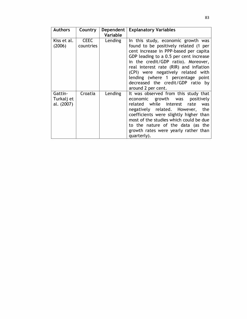
83



Kiss et al. (2006)

CEEC countries

Lending In this study, economic growth was found to be positively related (1 per cent increase in PPP-based per capita GDP leading to a 0.5 per cent increase in the credit/GDP ratio). Moreover, real interest rate (RIR) and inflation (CPI) were negatively related with lending (where 1 percentage point decreased the credit/GDP ratio by around 2 per cent.

Gattin-Turkalj et al. (2007)

Croatia Lending It was observed from this study that economic growth was positively related while interest rate was negatively related. However, the coefficients were slightly higher than most of the studies which could be due to the nature of the data (as the growth rates were yearly rather than quarterly).

84

CHAPTER 4 RELATIONSHIP BETWEEN FINANCIAL LIBERALISATION AND

EXCESS LIQUIDITY AT BANK-LEVEL

4.1 INTRODUCTION

Although there was no specific study on the relationship between financial

liberalisation and excess liquidity at bank-level according to our

knowledge, there were many works on excess liquidity at an aggregate

level. These were discussed earlier in detail in Chapter 3. From all these

works, it could be observed that these countries were still experiencing

significant amount of excess liquidity and it remained one of the focal

problems for most, if not all, of these developing economies.

To have an idea about the excess liquidity situation in Bangladesh, data of

nominal excess liquidity, real excess liquidity and excess liquidity as a

percentage of required liquid assets are given in Table 4.116. It could be

observed from the table that excess liquidity in nominal terms has

increased substantially. Since increase in the nominal excess liquidity could

in some part be attributed to inflation, therefore, excess liquidity data was

also provided in real terms. This helped in seeing the actual change and

trend of excess liquidity free from the effect of inflation. It could be seen

that real excess liquidity also increased over time.

Excess liquidity as a percentage of the required liquid assets (statutory

liquidity ratio, SLR) provided the relative excess liquidity situation for the

period of 1987-2011. The continuous overall increase of this ratio implied

that the rise in excess liquidity was not due to increase in the number of

banks or the number of branches because when the number of branches

increase then the amount of deposits also increase. As a result of which the

total amount of excess liquidity in the country might increase in absolute

terms. But when excess liquidity is taken as a ratio of required reserve,

then it will truly show the condition and trend of excess liquidity after 16 This was also provided earlier graphically in Figure 2.6.

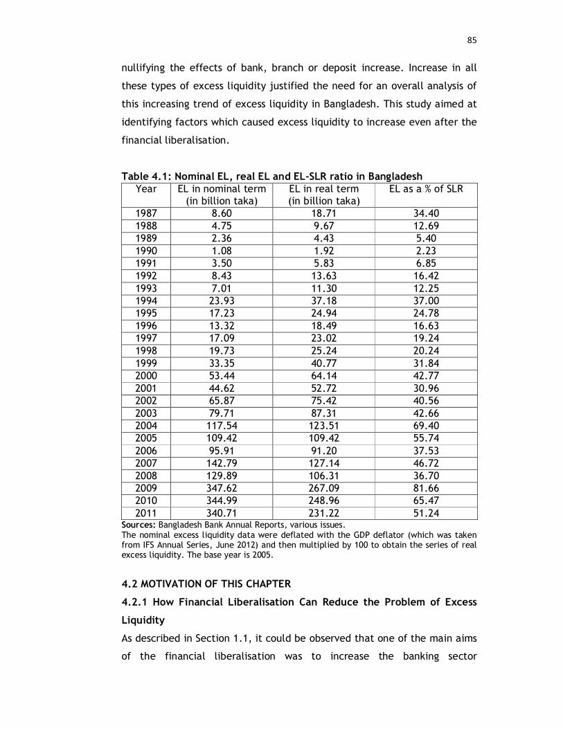
85

nullifying the effects of bank, branch or deposit increase. Increase in all

these types of excess liquidity justified the need for an overall analysis of

this increasing trend of excess liquidity in Bangladesh. This study aimed at

identifying factors which caused excess liquidity to increase even after the

financial liberalisation.

Table 4.1: Nominal EL, real EL and EL-SLR ratio in Bangladesh Year

EL in nominal term

(in billion taka) EL in real term (in billion taka)

EL as a % of SLR

1987 8.60 18.71 34.40 1988 4.75 9.67 12.69 1989 2.36 4.43 5.40 1990 1.08 1.92 2.23 1991 3.50 5.83 6.85 1992 8.43 13.63 16.42 1993 7.01 11.30 12.25 1994 23.93 37.18 37.00 1995 17.23 24.94 24.78 1996 13.32 18.49 16.63 1997 17.09 23.02 19.24 1998 19.73 25.24 20.24 1999 33.35 40.77 31.84 2000 53.44 64.14 42.77 2001 44.62 52.72 30.96 2002 65.87 75.42 40.56 2003 79.71 87.31 42.66 2004 117.54 123.51 69.40 2005 109.42 109.42 55.74 2006 95.91 91.20 37.53 2007 142.79 127.14 46.72 2008 129.89 106.31 36.70 2009 347.62 267.09 81.66 2010 344.99 248.96 65.47 2011 340.71 231.22 51.24

Sources: Bangladesh Bank Annual Reports, various issues. The nominal excess liquidity data were deflated with the GDP deflator (which was taken from IFS Annual Series, June 2012) and then multiplied by 100 to obtain the series of real excess liquidity. The base year is 2005.

4.2 MOTIVATION OF THIS CHAPTER

4.2.1 How Financial Liberalisation Can Reduce the Problem of Excess

Liquidity

As described in Section 1.1, it could be observed that one of the main aims

of the financial liberalisation was to increase the banking sector

86

competition. For this, these countries needed to deregulate interest rates,

privatise and liberalise bank licensing in order to increase competition,

lower the reserve requirements and dismantle any credit allocation

schemes (Goldsmith, 1969; McKinnon, 1973; Shaw, 1973). Moreover,

judicious private bankers, without the constraints of credit controls, would

allocate funds to the most productive users. These two together would lead

banks to lend more. Banks’ ability to give more credit would also imply

that there would be less liquidity in the banking sectors. In other words,

the financial liberalisation should substantially reduce the excess liquidity

situation.

4.2.2 Why Financial Liberalisation May Not Reduce the Problem of

Excess Liquidity and Rather Increase It

It needs to be taken into account that the process of financial liberalisation

was not an isolated process or phenomenon but it rather came with many

policies which have their own implications. It was observed by different

studies that the process of financial liberalisation could make an economy

more fragile and vulnerable because of its related policies. This fragility

and vulnerability could also lead to possible banking crises if the

institutions were not very strong (Detragiache and Demirguc-Kunt, 1998).

Authors also found that the risk in the banking system increased after

financial liberalisation (Fischer and Chenard, 1997). These could make the

economy less stable and banks may feel more uncertain. If banks were not

good at risk management in a more risky environment after the beginning

of financial liberalisation, then they might not lend enough. For a similar

reason, banks might also decide to keep their money in government bills

and bonds as they were risk-free and in most cases had reasonably high

rates of return. Banks also take note of the fact that due to the removal of

the ceiling of the interest rate (and an increase in the rate thereby), safer

borrowers apply less for loans and were replaced by the high-risk borrowers

(Blanchard and Fischer, 1989). This either led banks to lend to “projects

with lower probabilities of success but higher payoffs when successful”

(Stiglitz and Weiss, 1981) or banks might decide not to go for lending for

these risky projects and might end up having higher excess liquidity.

87

4.2.3 Stages and Sequencing of Financial Liberalisation

It was also found that the effect of the financial liberalisation can have

different impact on different countries depending on the stage of

liberalisation (Bandiera et al., 2000). This is due to the fact that financial

liberalisation is a continuous process and a country at its early stage may

not have the same impact like a country that is at an advanced stage of the

liberalisation.

Sequencing of financial liberalisation can play a vital role in achieving the

objectives of financial liberalisation. Moreover, institutional strength was

critically important for the success of it. Caprio et al. (2006) mentioned,

“institutional strengthening now widely accepted as being the pre-requisite

of a successful liberalised financial sector.” If an economy was structurally

weak then it was difficult to reap the benefits of financial liberalisation.

4.2.4 Importance of Bank-level Study

Another important contribution of this study was to see the relationship of

excess liquidity and financial liberalisation using various bank-specific

characteristics. While most of the studies on excess liquidity problem were

done on a specific country at an aggregate level (e.g. Agenor et al., 2004;

Fielding and Shortland, 2005; Chen, 2008; Zhang, 2009; Yang, 2010;

Aikaeli, 2011), very few examined this at a cross-country level. Most of

cross-country studies were done on Africa (Saxegaard, 2006; Khemraj,

2010).

According to our knowledge, there was no study on excess liquidity and

financial liberalisation at bank-level. In this respect, a study at bank-level

could provide important findings for the persistent excess liquidity. Bank-

level study could shed important light on how banks behaved in terms of

excess liquidity at bank-level. The bank-level study allowed us to look for

differences according to different typology of banks. Hence the evolving

pattern of excess liquidity with the process of financial liberalisation could

be seen more specifically for these different typologies.

88

The banks in Bangladesh have diverse characteristics and on the basis of

various criteria, could be classified into different groups. Based on the

existing literature, banks were classified according to ownership (whether

owned by the government or privately), size (if they were large or small),

mode of operation (whether Islamic or conventional/otherwise) and age

(whether new or old). Using data at bank-level, this study attempted to

investigate if banks behaved differently in terms of excess liquidity

according to these characteristics17.

This approach could shed important light on the behavioural and

operational characteristics and effectiveness of the different types of

banking system within a same country and how they adapted and

benefitted from financial liberalisation. Antwi-Asare and Addison (2000)

observed that bank-specific indicators could be important in showing the

different effects of bank performance. These differences among them

could have different effects of the financial liberalisation.

It was generally observed that private banks were more efficient than

public banks. In a study on Pakistan, the authors used the group-wise

efficiency and found that as a group, the private domestic banks had 90.5

per cent efficiency while the nationalised commercial banks had 70.5 per

cent (Abbas and Malik, 2010). In another study on Ghana, it was found that

the state-run banks were not prepared to take as much risk when lending

as the private banks (Antwi-Asare and Addison, 2000). The authors

observed that the performances of the private banks were higher than the

state-owned banks in terms of profitability, intermediation and operations.

However, the above view was not always found to be true. Das and Drine

(2011) found that public sector banks were more efficient than the

domestic private banks in India.

17 In this study, the foreign commercial banks could not be included due to lack of bank-level data for foreign banks operating in Bangladesh. Bureau van Dijk – producer of the Bankscope database, which is one of the most comprehensive database of banks operating throughout the world and is the main source of data for this study – was contacted directly but they confirmed that they did not have data at bank-level for foreign banks in Bangladesh.

89

Generally it was seen that new banks performed better in times of financial

liberalisation. One possible reason, mentioned by Kraft and Tirtiroglu

(1998), was that since they were not held back by overstaffing or bad loans.

However, the empirical results did not always support this view and in

some cases it was found that old banks performed better than the new

banks. One possible explanation could be their advantage in terms of size

and experience, helping them to work nearer to efficient scale and at a

comparable or better level of managerial efficiency than the new banks

(Kraft and Tirtiroglu, 1998).

The possible effect of financial liberalisation on Islamic banking was still

ambiguous. On one hand, there was perception that Islamic banks could not

take full advantage of the financial liberalisation as they were

comparatively small, narrow in focus and mostly vulnerable to financial

shocks. On the other hand, it was also believed that Islamic banks were

able to cope better with the vulnerability and the fragility caused by the

financial liberalisation. So, whether financial liberalisation had a positive

effect on Islamic banking remained inconclusive (Bashir, 2007).

Inability to reach a definitive conclusion was also evident when the possible

effect of financial liberalisation on bank size was analysed in the literature.

Some argued that large banks performed better in times of financial

liberalisation (Berger and Humphrey, 1997; Yildirim, 2002; Andries and

Capraru, 2013). The main possible reason for this was the market power of

‘larger banks’ and their ability to diversify credit risk in an uncertain

macroeconomic environment (Yildirim, 2002). Nevertheless, some others

had observed that smaller banks were more efficient than the larger ones

(Leong and Dollery, 2002). This “could be due to their higher flexibility,

which allowed them to adapt to changes in the banking industry brought

about by the financial liberalisation programme” (Ataullah et al., 2004).

Therefore, it would be interesting to see if these differences in

characteristics in the banking sector had any effect on excess liquidity.

Guha-Khasnobis and Mavrotas (2008) mentioned that country-specific

90

studies could be very useful for a more in-depth analysis. Therefore this

study would analyse these aspects of ownership, size, mode of operation

and age of the banking sector in Bangladesh.

4.2.5 Contribution of this Chapter

Financial liberalisation in Bangladesh was initiated in the early 1980s. But

this was not a one-step process. Three distinct sectors were identified in

which financial liberalisation took place. These were: (a) development of

competitive banking sector and a viable rural financial system; (b) control

over interest rate, exchange rate and capital flows; and (c) development of

money and capital market. Financial liberalisation in these three sectors

did not take place simultaneously. In fact, it was not until 1990 that the

process of financial liberalisation started in the case of interest rates. This

was observed with the departure of nominal interest rates and the interest

rate spread from the regimentally fixed round values after 1990 (Hossain,

1996). Regarding the interest rate liberalisation, Mujeri and Younus (2009)

wrote:

“Bangladesh began to implement financial sector reform

measures in the 1980s and the interest rates were partially

deregulated in November 1989 to introduce flexibility in

determining deposit and lending rates. As a part of the

process, Bangladesh Bank started to set the ceilings and the

floors and individual banks were allowed to set their interest

rates within the stipulated band. In April 1992, the interest

rate bands for lending were removed for all sectors except

agriculture, small industries and exports while, for deposits,

the ceilings were removed but the floors were retained.”

It could be observed from Table 4.1 that excess liquidity in Bangladesh had

a general growing pattern over time. One point that needed to be noted

was that excess liquidity fell before the financial liberalisation programme

but it increased, with some exceptions, after the financial liberalisation.

This put forward the need for a study which could explain the reasons for

this continuous increasing trend. It could either be due to the financial

91

liberalisation itself or it could be because of the standard factors used in

earlier studies of excess liquidity or could be a combination of both.

Therefore, the standard variables along with financial liberalisation was

applied in this study to see why excess liquidity was so high and still

increasing in Bangladesh.

As mentioned before, there was no study using bank-level data to directly

look at the relationship between financial liberalisation and excess liquidity

directly according to our knowledge. To fill this vacuum in the literature,

bank-level data were used to examine how excess liquidity and the

financial liberalisation were related.

As the study period of this paper started after the financial liberalisation

was initiated in Bangladesh, hence an index of financial liberalisation

(introduced in Section 4.3.2.1) was used to properly capture the effect of it

on excess liquidity. It not only allowed a quantitative study of their

relationship but also helped in reaching towards a definitive conclusion

about the continuous and ever growing debate of the effect of the financial

liberalisation and attainment of its objectives.

4.3 THE EMPIRICAL APPROACH

4.3.1 Dependent Variable

The dependent variable for this study was excess liquidity. This was

measured using the liquid assets data from Bankscope. It was calculated in

Bankscope by summing up: trading securities and at fair value (FV) through

income, loans and advances to banks, reverse repos and cash collateral and

cash and due from banks. Then mandatory reserves included above were

deducted. Finally, growth of this was taken.

4.3.2 Explanatory Variables

One of the main variables of interest in this study was financial

liberalisation. Other key variables of interest were the bank typology

variables. These were included to see if there was any pattern among

different types of banks in terms of excess liquidity due to financial

92

liberalisation. Moreover, the standard variables in the excess liquidity

literature were also incorporated to see the direction and significance of

their relationship. These standard variables included deposit volatility,

interest rate, government bill and bond rate as well as the lagged

dependent variable. The measurements of these determinants in the

context of bank-level study of excess liquidity are discussed in the

following pages.

4.3.2.1 Standard Control Variables

Deposit volatility: Liquidity preference of banks was affected by the public

expectations formation. This was found to be related with excess liquidity.

Agenor et al. (2004) found this as one of the main factors that could

explain the excess liquidity problem for the economy of Thailand. Larsen

(1951) also identified this as a probable reason for excess liquidity.

According to him, liquidity preference of banks was affected by public

expectations. To analyse demand for liquidity of banks, volatility of

depositors’ cash preference should thus be taken into consideration.

Saxegaard (2006) observed that currency withdrawal volatility, which was

very similar to deposit volatility, could influence excess liquidity situation.

From Bankscope, the data of total deposits or total customer deposits

could represent the concept of deposit. These measures could also

represent concepts like excess savings (that was used by Gu and Zhang,

2006; Wang, 2006; McKinnon, 2006, 2007; Han and Chen, 2007; Roubini,

2007; Xia and Chen, 2007; Zheng and Yi, 2007; Chen, 2008) and low

consumer spending (which was used by Qing, 2006; Jiao and Ma, 2007).

Moreover, deposit volatility also represented the liquidity risk (Agenor et

al., 2004) since the volatility of deposit might force banks to keep more

liquid assets than required due to the uncertainty involved.

In this study, the volatility of deposit was measured by a 3-year period

standard deviation of total deposit using the overlapping method. Reason

for choosing the 3-year period was the short span of data availability as the

maximum period of available data for each bank was 15 years. Through this

93

way, two observations were lost but still there were generally a series of

13 years of data for each bank.

Deposit rate: The deposit rate could affect the excess liquidity situation of

the banks. If the deposit rate was high, people would be more interested in

keeping their money in banks. Assuming everything else constant, this

would lead to higher level of excess liquidity in the banking sector. Hence,

it could be assumed that the deposit rate would be positively related with

the excess liquidity situation of the banking sector. From Bankscope, the

ratio of interest expense on customer deposits as a ratio of average

customer deposits was taken to measure this variable.

Impaired loans: One possible reason of high impaired loans was risky

environment. If banks faced problem of loan default, then they would be

less encouraged towards lending which will lead towards less allocation of

credit. Hence, the amount of impaired loans could lead to higher excess

liquidity. Impaired loans as a ratio of gross loans data from Bankscope was

taken to measure this determinant. This measure might also represent

factors like weak contract enforcement and rule of law as well as

imprudent lending.

Government bills and bonds: As discussed earlier, out of the total required

reserve for each bank, some part was needed to be kept in cash. This was

called the CRR. The rest could be put in cash or in government bills or

bonds. Since these were risk free, so there was a tendency of banks to put

part of their reserves in the government bills and bonds rather than opting

for lending as that involved risk of default. The rate of these bills and

bonds and their difference with the lending rate played a significant role

on how much would be invested on these as well as the direction and

significance of the relationship.

In this respect, the spread between the treasury bill rate and the lending

rate was applied to see how it affected the excess liquidity situation. This

measure involved both the rates that banks consider and decide whether to

94

invest or keep as liquid assets. Treasury bill rate for the 91-day bills was

used to represent the government bills and bonds. Then the lending rate

was deducted from this rate for each individual bank. The lending rate was

proxied by the ‘interest income/ average earning assets (%)’ measure from

Bankscope.

Lagged dependent variable: The lag of excess liquidity was used in some

of the earlier studies of excess liquidity (e.g. Agenor et al., 2004;

Saxegaard, 2006; Aikaeli, 2011). The reason for using this as one of the

explanatory variables was that it takes into account both the

contemporaneous and the lagged effects. Another argument for its

inclusion was that the adjustments were unlikely to be instantaneous.

Hence, one-year lag values of the dependent variable were taken as one of

the explanatory variables.

Some other variables: Some variables that were used in earlier studies but

not included in this work due to their similarity with one of the

independent variables or the dependent variable are described here. The

rate of required reserve was observed as one of the important variables in

earlier studies. However, since the dependent variable in its definition

deducts the mandatory reserve, hence the required reserve variable was

not included as one of the explanatory variables. The concepts of ‘excess

savings’, ‘low consumer spending’ and ‘liquidity risk’ could be measured by

the same measure of ‘deposit volatility’ concept while the concept of

‘weak credit growth in relation to domestic deposit growth’ was very close

to the concept of excess liquidity. Since deposit rate was used as an

explanatory variable and lending rate was used to measure the spread from

the treasury bill rate, so the ‘lending rate’ and ‘interest rate spread’ were

not used separately. Different external factors like ‘foreign reserve’,

‘export’, ‘foreign aid’, ‘oil revenue’, ‘foreign direct investment’,

‘exchange rate’ and ‘remittance’ were described important in different

earlier studies (e.g. Gilmour, 2005; IMF, 2005; Khemraj, 2006; Qing, 2006;

Saxegaard, 2006; Jiao and Ma, 2007; Ma 2007; Bakani, 2012). At bank-level

several of these are irrelevant. One measure that might be able to proxy

95

the variable of exchange rate was deposit rate since central bank could

enforce a higher deposit rate for each bank to protect the economy from a

weak exchange rate. Since deposit rate was used as one of the explanatory

variables, exchange rate was not separately included in this study.

4.3.2.2 Key Variables of Interest

Financial liberalisation: In different works, financial liberalisation was

represented by different variables or measures. Generally, easily available

monetary aggregates such as M2 or M3 as a ratio of nominal GDP were

widely used (Ang and McKibbin, 2007). Using dummy variable for financial

liberalisation was also a very common practice. However, since financial

liberalisation was a continuous process including many reversals, it was

very difficult to capture this process with only a 0 or a 1. Moreover, it

involved many processes together and also the process was an on-going

one. Keeping this in mind, there has been a recent trend to build index of

financial liberalisation where different processes of financial liberalisation

were combined together and the magnitudes of those processes could also

be incorporated (e.g. Williamson and Mahar, 1998; Bandiera and others,

2000; Edison and Warnock, 2003; Kaminsky and Schmukler, 2003; Laeven,

2003).

In one of these new initiatives, Abiad et al. (2010) formed an index of

financial liberalisation where they distinguished seven different dimensions

of financial liberalisation. These dimensions were: credit controls and

excessively high reserve requirements, interest rate controls, entry

barriers, state ownership in the banking sector, capital account

restrictions, prudential regulations and supervision of the banking sector

and securities market policy (these seven dimensions are discussed in detail

in Appendix 4.5).

Following this, an index of financial liberalisation was constructed for

Bangladesh for the period of 1997-2011. In every dimension, one or more

questions were used and they were coded afterwards to see the overall

impact of the financial liberalisation. In the first dimension of ‘credit

96

controls and excessively high reserve requirements’, the questions were:

1)Were reserve requirements restrictive? 2) Were there minimum amounts

of credit that must be channeled to certain sectors? 3) Was any credit

supplied to certain sectors at subsidised rates? 4) Were there in place

ceilings on expansion of bank credit?

In the second dimension of ‘interest rate liberalisation’, deposit rates and

lending rates were separately considered. Factors included if both deposit

interest rates and lending interest rates were determined at market rates

or they were fixed within a band.

‘Banking sector entry’, which was the third dimension, included the

following four questions: 1) To what extent did the government allow

foreign banks to enter into a domestic market? 2) Did the government allow

the entry of new domestic banks? 3) Were there restrictions on branching?

4) Did the government allow banks to engage in a wide range of activities?

The fourth dimension of ‘capital account transactions’ included the

questions of: 1) Was the exchange rate system unified? 2) Did a country set

restrictions on capital inflow? 3) Did a country set restrictions on capital

outflow?

The fifth dimension of ‘privatisation’ examined the magnitude of

privatisation of banks. ‘Securities markets’, which was the sixth dimension,

included the following two questions: 1) Had the country taken measures to

develop securities markets? 2) Was the country’s equity market open to

foreign investors?

The last dimension of this index was the ‘banking sector supervision’. This

had four questions: 1) Had the country adopted a capital adequacy ratio

(CAR) based on the Basel standard? 2) Was the banking supervisory agency

independent from executives’ influence? 3) Did a banking supervisory

agency conduct effective supervisions through on-site and off-site

97

examinations? 4) Did the country’s banking supervisory agency cover all

financial institutions without exception?

As could be noted from the different dimensions and sub-dimensions, some

of these were quantitative while some were qualitative. For the

quantitative ones, the published data sources were used. Regarding the

qualitative ones, different information from various sources was used for

this purpose. After collecting all the information and providing a

quantitative value for each one irrespective of whether they were

quantitative or qualitative, they were checked with the Abiad et al.

database of Bangladesh for the period available (1997-2005). It was found

that this new database generally conformed to the Abiad et al. (2010)

database.

One difference between the Abiad et al. (2010) index and financial

liberalisation index measure of this study was that while Abiad et al. (2010)

rescaled their dimensions in creating the final index, here the dimensions

were not rescaled after summing up the values of each sub-dimension. The

reason behind not rescaling was that this could suppress the effects of the

process of financial liberalisation and then the estimates would not fully

reflect the effects of this process.

Bank typology: To see if there were any effect of different types of banks

on excess liquidity due to the process of financial liberalisation, the banks

in Bangladesh in this study were classified according to ownership (whether

owned by the government or private), size (whether they have assets over

$1 billion or not), mode of operation (whether run according to Islamic

principles of banking or otherwise) and age (whether they were new or old).

Although there was no universal definition for the classification of bank

size, the rule followed in this study has also been used in many earlier

studies (e.g. Cole et al., 2004) including works on Bangladesh (e.g. Cihak

and Hesse, 2008). If (and when) banks have assets over $1 billion, the size

98

dummy was 1 and 0 otherwise18. There can be other approaches such as

classifying them as big or small on the basis of data at the beginning of the

sample, or at the end of the sample, or as averages over the entire sample.

However, the approach taken in this study was more reflective of the

actual situation as with this approach, there were some banks which have

value of 0 in some years and 1 in some other years as they moved from

small to large. For banks which remain either in the large or in the small

category, have one static value (of either 0 or 1) for the whole study

period. For the ownership dummy, the value of 1 was taken if the bank was

owned by the state and 0 otherwise. For the dummy value for mode of

operation, it was 1 if it operates according to the Islamic principles of

banking and 0 otherwise19. For the age dummy the value was 1 if they were

in the new category (established after 1990) and 0 otherwise. All these

dummy values were multiplied by the financial liberalisation index value

and these multiplied variables were used in the estimation. A table was

given here based on the above characteristics.

Earlier works on holding liquid assets started where the cost of having or

holding liquid assets, which had lower return than other investments, was

compared with the risks of running out (Baltensperger, 1980; Santomero,

1984). This implied that if the risk of running out was higher, then banks

would incur the cost of holding excess liquidity. Therefore, excess liquidity

situation and decision of bank would depend on the opportunity cost of

holding liquid assets. According to the newer generation of models, market

imperfections play a key role for banks being unable to raise instantaneous

and unlimited amounts of liquidity. These imperfections were generally

referred to as moral hazard (Holmstrom and Tirole, 1998) or adverse

selection (Kiyotaki and Moore, 2008). Therefore, financially constrained

banks would try to have more liquidity.

18 Due to the growth of the banking sector, many banks moved from small to large category over the study period. Each bank was categorised accordingly by giving a value of 0 when their assets was less than $1 billion while 1 when they cross this mark. 19 There are some banks which had some branches or sections operating under Islamic principles of banking. In this study, only those banks were included under Islamic banking category which used Islamic principles of banking throughout.

99

Table 4.2: Bank classifications

Sl. No.

Name of bank Bank ownership

Bank size

Bank mode of operation

Bank age

Year of

start 1. AB Bank Private Small to

Large Conventional Old 1982

2. Agrani Bank Public Large Conventional Old 1971 3. Al-Arafah

Islami Bank Private Small to

Large Islamic New 1995

4. Bangladesh Commerce Bank

Public Small Conventional New 1999

5. Bangladesh Development Bank

Public Small Conventional Old 1971

6. Bangladesh Krishi Bank

Public Small to Large

Conventional Old 1971

7. Bank Asia Private Small to Large

Conventional New 1999

8. BASIC Bank Public Small Conventional Old 1988 9. BRAC Bank Private Small to

Large Conventional New 2001

10. City Bank Private Small to Large


11. Dhaka Bank Private Small to Large


12. Dutch Bangla Bank

Private Small to Large


13. Eastern Bank Private Small to Large


14. EXIM Bank Private Small to Large

Islamic New 1999

15. First Security Islami Bank


Islamic New 1999

16. ICB Islamic Bank Limited

Private Small Islamic Old 1987

17. IFIC Bank Private Small to Large


18. Islami Bank Bangladesh


Islamic Old 1983

19. Jamuna Bank Private Small to Large


20. Janata Bank Public Large Conventional Old 1971 21. Mercantile

Bank Private Small to

Large Conventional New 1999

22. Mutual Trust Bank

Private Small Conventional New 1999

23. National Bank Private Small to Large


24. NCC Bank Private Small to Large


100

Sl. No.

Name of bank Bank ownership

Bank size

Bank mode of operation

Bank age

Year of

start 25. One Bank Private Small Conventional Old 1999 26. Premier Bank Private Small Conventional Old 1999 27. Prime Bank

Limited Private Small to


28. Pubali Bank Private Small to Large

Conventional Old 1983*

29. Rupali Bank Public Small to Large


30. Shahjalal Islami Bank


Islamic Old 2001

31. Social Islami Bank


Islamic Old 1995

32. Sonali Bank Public Large Conventional Old 1971 33. Southeast

Bank Private Small to


34. Standard Bank

Private Small Conventional Old 1999

35. Trust Bank Private Small Conventional Old 1999 36. United

Commercial Bank



37. Uttara Bank Private Small to Large

Conventional Old 1983*

Source for size: Defined according to total asset data from Bankscope. Source for ownership, mode of operation and age: BB Annual Report, various issues. *Uttara Bank and Pubali Bank were denationalised to operate as Private Commercial Bank. Note: Small to Large means that asset of the bank was lower than $1 billion at the beginning but crossed the threshold at some point during this period.

Earlier works on holding liquid assets started where the cost of having or

holding liquid assets, which had lower return than other investments, was

compared with the risks of running out (Baltensperger, 1980; Santomero,

1984). This implied that if the risk of running out was higher, then banks

would incur the cost of holding excess liquidity. Therefore, excess liquidity

situation and decision of bank would depend on the opportunity cost of

holding liquid assets. According to the newer generation of models, market

imperfections play a key role for banks being unable to raise instantaneous

and unlimited amounts of liquidity. These imperfections were generally

referred to as moral hazard (Holmstrom and Tirole, 1998) or adverse

selection (Kiyotaki and Moore, 2008). Therefore, financially constrained

banks would try to have more liquidity.

101

Based on these models, bank characteristics, such as bank size and

ownership, could affect their ability to raise non-deposit forms of finance.

For example, small banks had more difficulties in accessing capital markets

while public banks were less liquidity-constrained than private banks, as

public banks might have an implicit guarantee. This would affect the

banks’ precautionary demand for liquidity buffers.

Kashyap and Stein (1997) and Kashyap et al. (2002), using a large panel of

US banks, found a strong effect of bank size on holdings of liquid assets

with smaller banks being more liquid as they face constraints in accessing

capital markets. Dinger (2009) also found that smaller Eastern European

banks hold more liquidity. However, Aspachs et al. (2005) did not find any

significant relationship between excess liquidity and bank size in their

panel study of 57 UK resident banks.

Bank age might also be related to performance, since bank production20

might follow the ‘learning by doing’ hypothesis (Mester, 1996). This would

imply that over time, performance of banks would improve as they would

learn new things and would adapt to the changing environment more than

before. However, it might also happen that efficient management might

become less prominent at some stage and opt for a less proactive style,

leading to a decrease in efficiency (Esho, 2001). If the latter effect

dominates then the age variable should display a positive coefficient.

Staikouras et al. (2007) found that the coefficient of the age variable was

positive and statistically significant in all specifications, in contrast to the

‘learning by doing’ hypothesis, as identified by Mester (1996), DeYoung and

Hasan (1998) and Kraft and Tirtiroglu (1998). They also mentioned that

older banks were mostly formerly state-owned.

20Banks’ ability to ameliorate informational asymmetries between borrowers and lenders and their ability to manage risks are the essence of bank production (Hughes and Mester, 1998). These abilities are integral components of bank output and influence the managerial incentives to produce financial services prudently and efficiently.

102

Demetriades and Fielding (2009) found that, for very young banks, raising

deposits was likely to be easier than identifying reliable borrowers. Older

banks were likely to have more information so that their ability to screen

borrowers was likely to be better than that of younger banks.

DeYoung (1999) found that bank age influenced the risk of small-bank

failure, especially if the banks were three to five years old because it took

some time for profits to reach a sustainable levels. Amel and Prager (2013)

measured this variable as the number of years since the bank opened. They

found it negative and significant for most cases in the rural regions, but its

sign varied over time in urban markets.

It was observed in different studies that Islamic banks generally had less

excess liquidity than the conventional banks (Gafoor, 1995; Siddiqui, 2013).

Initially this was due to less people being attracted towards this new

banking system to deposit money. On the other hand, Islamic banking

system had fewer instruments than the conventional banking to lend money

(Siddiqui, 2013). Over time, more people became interested in the Islamic

system of banking and the difference between this type of banking with

conventional banking reduced significantly. However, like the conventional

banks, Islamic banks in Bangladesh were also suffering from this problem of

excess liquidity.

4.3.3 Variations According to Bank-specific Characteristics

Two different strategies were applied here to see if there were any

possible differences in excess liquidity according to bank-specific

characteristics of ownership, size, mode of operation and age. Firstly,

various graphs of the time-evolution of average excess liquidity were drawn

splitting the data based on these characteristics. These were done

separately as the characteristics were not exclusive from each other.

Therefore, four separate graphs were drawn to see visually if there were

any variations among them. Secondly, statistical tests were applied

according to these characteristics to see if they differed from each other.

These tests included both nonparametric and parametric tests.

103

4.3.3.1 Variations According to Graphs

Figure 4.1 shows the excess liquidity for public and private banks.

Figure 4.1: Excess liquidity according to ownership

Sources: Author’s own calculation based on data from Bankscope and Bangladesh Economic Review, various issues.

It could be seen from the figure that there were differences in excess

liquidity between public and private banks. The gap increased in the late

90’s but started converging from the early 2000. They remained quite close

from 2005 onwards. It could also be observed that while the private banks

experienced a fluctuating pattern, the public banks had a rather steady

pattern over the period.

Large and Small Banks

Figure 4.2 shows if there was any difference between large and small

banks. It could be seen from the figure that there was difference between

large and small banks also and the trend was quite similar with the gap

increasing in the late 90’s but starting to converge from the early 2000s.

They remained quite close from 2005 onwards. It could also be observed

that while the large banks experienced a fluctuating pattern, the small

banks had a rather steady pattern over the period.

0

0.1

0.2

0.3

0.4

0.5

0.6

Average Public Banks

Average Private Banks

104

Figure 4.2: Excess liquidity according to size


Islamic and Conventional Banks

In contrast to the earlier two characteristics, Figure 4.3 showed that excess

liquidity of Islamic banking and conventional bankingwasquite similar.

Figure 4.3: Excess liquidity according to mode of operation

Sources: Author’s own calculation based on data from Bankscope and Bangladesh Economic Review, various issues

Although the gap increased in the late 1990s, they remained quite close

from 2000 onwards. The trend of their change also remained quite similar

0

0.1

0.2

0.3

0.4

0.5

0.6

Average Large BanksAverage Small Banks

0

0.1

0.2

0.3

0.4

0.5

0.6

0.7

Islamic Banks

Conventional Banks

105

over these years where increase and fall followed a very analogous pattern.

However, the pattern of the conventional banks fluctuated less than that

of the Islamic banks.

New and Old Banks

The characteristic of age seemed to follow a similar pattern of differences

as were observed for ownership and size. Starting with a substantial gap at

the beginning of the study period, the gap increased substantially.

However, over the years it fell markedly and remained quite close from

2005 onwards. It could also be observed that while the new banks

experienced a fluctuating pattern, the old banks had a rather steady

pattern over the period.

Figure 4.4: Excess liquidity according to age

Source: Author’s own calculation based on data from Bankscope and Bangladesh Economic Review, various issues.

4.3.3.2 Statistical Tests for Difference among Bank Typologies

Two types of statistical tests were carried out in addition to the graphical

representation above. The first type of test was a non-parametric test

while the second type of test was a parametric test. The non-parametric

test applied was the Wilcoxon rank-sum test whereas t-test was applied as

the parametric test.

0

0.1

0.2

0.3

0.4

0.5

0.6

0.7

0.8

Average Old BanksAverage New Banks

106

The Wilcoxon rank-sum test, also called the Wilcoxon Mann-Whitney test,

was a nonparametric test for assessing whether two samples of

observations came from the same distribution. This was applied for two

unmatched group of observations (Wilcoxon, 1945; Mann and Whitney,

1947). The null was that the two populations had identical distribution

functions against the alternative hypothesis was that the two distribution

functions differed21.

It is one of the most powerful nonparametric tests. This test does not

require the assumption that the differences between the two samples be

normally distributed. It was also frequently used as an alternative of the

two sample t-test when the normality assumption was questionable 22 .

Janusonis (2009) stated that Wilcoxon test should not be applied if one

group had 3 and the other group had 3 or 4 cases and t-test was better with

sample size of N = 3 or N = 4. Posten (1982) found that for sample sizes of

as small as 5 per group, Wilcoxon test had the highest statistical power23.

For the Wilcoxon rank-sum test, there were two independent random

variables, and , and the following null hypothesis of ~ was tested

with a sample size of for and for . In this test, the null

hypothesis was that there was no difference between the two (unmatched)

groups. If the null was rejected (when the probability was less than 10% or

0.1), then it implied that there was significant difference between the

groups.

The results of the Wilcoxon rank-sum test across bank typologies were

given below with the null hypothesis that there was no difference between

two groups. Here, excess liquidity was the ranking variable.

21 The Mann-Whitney-Wilcoxon (MWW) U-test was an extension of the Wilcoxon (1945) test that was developed for equal sample sizes. 22 The following website contained further details: http://www.stats.gla.ac.uk/steps/glossary/nonparametric.html#wmwt 23 For detailed discussion and comparision between these tests, see de Winter (2013).

107

The Wilcoxon rank-sum test results showed that the null of no difference

for ownership typology was rejected implying that there was difference

between public and private banks in terms of excess liquidity. Similar

findings were observed for both size and age typology suggesting that there

was variation between large and small banks as well as between new and

old banks. However, the null for the mode of operation typology was not

rejected implying that there was no significant difference between Islamic

and conventional banks in terms of excess liquidity.

Table 4.3: Wilcoxon rank-sum test results for bank typologies of


Typology Ownership observation rank sum

expected H0: no difference between two (unmatched) groups

Ownership

Private 30 649 570 3.064

(0.0022) Public 7 54 133

Size Large 6 207 114 3.132

(0.0017) Small 31 496 589

Mode of

operation

Islamic 7 166 133 -1.280

(0.2006) Conventional 30 537 570

Age New 21 277 399 3.740

(0.0002) Old 16 426 304

The parametric tests applied here was the t-test. The results of the t-test

conform to the findings of the Wilcoxon rank-sum test, showing that there

were differences for all the bank-specific characteristics except the mode

of operation typology.

The results of this test are provided here. The results showed that the

coefficient of ownership, age and size were significant at 1% level while

that of the mode of operation was not.

108

Table 4.4: t-test results for excess liquidity according to ownership,

size, mode of operation and age

Typology Coefficient Standard

error

z P > | z | 95% confidence

interval

Ownership

-0.114 0.027 -4.23 0.000 -0.166 -0.061

Size -0.108 0.030 -3.60 0.000 -0.167 -0.049

Mode of

operation

0.049 0.033 1.49 0.137 -0.015 0.113

Age 0.099 0.020 4.97 0.000 0.060 0.138

4.4 METHODOLOGY

This study used panel data. This type of data has three main advantages

over cross-section data. Firstly, it can exploit both cross-section and time

series variation in the data. Secondly, this technique can control for the

presence of unobserved firm-specific factors (in this case, bank-specific

factors). Finally, this approach can also address the problem of potential

endogeneity of the regressors (Verbeek, 2004).

In this panel data analysis, there might be unobserved bank-specific time-

invariant heterogeneity, which could bias the estimates if not properly

accounted for. This was due to the fact that the error term might contain

time varying bank-specific characteristics which might be correlated with

banks’ liquidity ratios. Another issue was potential endogeneity of some of

the explanatory variables.

These concerns could be addressed with the GMM proposed by Arellano and

Bond (1991), Arellano and Bover (1995) and recently extended by Blundell

and Bond (2000) and Bond (2002). This method was particularly appropriate

to address the dynamic panel bias that arised in the presence of lagged

dependent variables in samples with a large number of groups (N) and a

relatively small number of time periods (T), such as in this study. This

method also helped to overcome the weak instrument problem (past

109

changes do contain information about current levels), and resulted in

improvements in the efficiency of the estimates (Arellano and Bond, 1991;

Roodman, 2006).

Another advantage of this framework was that it helped to control for

potential biases induced by endogeneity (the correlation between the

lagged dependent variable and the error term) which was inherent in the

specification because of the inclusion of lagged dependent variables as

regressors.

However, Roodman (2009) argued that the system GMM could generate

moment conditions prolifically, in which case, too many instruments in the

system GMM overfits endogenous variable and weakens the Hansen test of

the instruments’ joint validity. Following Zulkefly et al. (2010), this study

adopted two techniques to remedy the problem of instruments

proliferation. First, not all available lags for instruments were used.

Second, instruments were combined through addition into smaller sets by

collapsing the block of the instrument matrix. This technique was also used

by Calderon et al. (2002), Cardovic and Levine (2005) and Roodman (2009),

among others.

The study used two-step system GMM estimation. Zulkefly et al. (2010)

argued that the success of the GMM estimator in producing unbiased,

consistent and efficient results was highly dependent on the adoption of

the appropriate instruments. Therefore, the following two specifications

tests were conducted as suggested by Arellano and Bond (1991), Arellano

and Bover (1995) and Blundell and Bond (1998). Firstly, the Hansen test of

overidentifying restrictions, which test the overall validity of the

instruments by analysing the sample analogue of the moments conditions

used in the estimation process. If the moment condition holds, then the

instrument was valid and the model is correctly specified. Secondly, the

nonserial correlation among the transformed error term was tested. The

AR(2) test for serial correlation was used for this.

110

Duprey (2013) mentioned that system GMM also has, among others, the

following advantages:

(i) It can limit the number of missing observations by using the forward

orthogonal deviation transform instead of the first difference

transformation, and

(ii) The use of the collapsed option was allowed which help to avoid the

proliferation of instruments, as all available lags were used as

internal instruments.

The estimated equation in this study mainly stemmed from the earlier

works of Agenor et al. (2004) and Saxegaard (2006). Additionally, financial

liberalisation index was added to see how it was related with excess

liquidity. Furthermore, interaction of bank typologies (BT) with the

financial liberalisation variable was included to see if there was any

difference in the behaviour of banks according to their characteristics. The

main equation of excess liquidity to be estimated in this study can be

simply written as:

= + , + + + + + ( ) +

( × ) + (4.1)

The above equation explains effect at bank-level on excess liquidity where

represented excess liquidity, was for deposit volatility, showed

interest rate, government bill and bond was given by , impaired loan

was represented by , expressed financial liberalisation index and BT

showed different bank typologies (ownership, size, mode of operation and

age). The interaction terms of FL and BT showed bank typologies based on

bank-specific characteristics interacted with the financial liberalisation

index. Banks were represented by subscript and was showing year.

The above model can be rewritten in a panel data framework in matrix

notation in the following way:

= + , + ′ + (4.2)

111

Here excess liquidity was shown with vector and was denoted as which

implied excess liquidity of bank in year ; was a parameter to be

estimated with respect to the lagged dependent variable (excess liquidity);

′ was a (1 × ) vector of regressors, was a (1 × ) vector of parameters

to be estimated and was the stochastic disturbance term.

According to the literature, when numerous individual units were observed

over time, specifying the stochastic nature of the disturbances became

conceptually difficult (Nerlove, 1971). For example, some of the ‘omitted

variables’ might reflect factors which were peculiar to both the individual

banks as well as the time periods for which the observations were

obtained. Others may reflect only those bank-specific differences which

affect the observations for a given bank while some variables may

represent factors which were peculiar to specific time periods (Owusu-

Gyapong, 1986).

Nerlove (1971) observed that if these unobservable ‘other effects’ were not

taken account of in the estimation process and ordinary least squares

method was applied to equation (4.2), then the estimates of the ’s in this

equation might be both biased and inefficient. Therefore, equation (4.2)

needed to be transformed to the following error component model to

include these other causal variables:

= + , + ′ + (4.3)

where,

= + = − − , − ′ (4.4)

and,

[ ] = [ ] = [ + ] = 0 (4.5)

Here, denote the unobservable individual specific effects and was time-

invariant, accounting for the special effects that were not included in the

model – the fixed effects. The remainder disturbance varies with both

individual and time – the idiosyncratic shock. The error of the model

112

therefore becomes the sum of , the individual specific effects, and ,

the well-behaved error component. It was assumed that and were

independent for each over all .

Although there were various methods of estimation for panel data, over

time it has been observed that the system Generalised Method of Moments

(system GMM)24 was superior to the fixed effects and the random effects

methods. There were some advantages of Generalised Method of Moments

over other panel estimators for specific cases. Firstly, this method does not

need distributional assumptions like normality. Secondly,

heteroscedasticity of unknown form was allowed in this model. Thirdly,

even if the model was not solvable analytically from the first order

condition, still the method can estimate the parameters (Verbeek, 2004).

From the above discussion, it could be concluded that the most appropriate

method was system GMM for the type of model (dynamic with short time

dimension) used in this study (Blundell and Bond, 1998). This method was

also applied in several empirical studies of similar types. This included

works of Cottarelli et al. (2003), IMF (2004) and Louzis et al. (2011).

If the lagged dependent variable was included to account for dynamics in

the process, then, methods like OLS, FE or Within Group (WG) estimators

contained some limitations. If OLS was applied, then the estimator would

be biased due to the presence of lagged dependent variables as one of the

explanatory variables. The bank-specific effects could be accounted for by

the FE or WG estimator but they would remain biased in the presence of

lagged dependent variables. This study therefore used the system GMM

estimator developed for dynamic panel data estimation25.

24 System GMM is proposed and continuously developed with the pioneer works of Arelleano and Bond (1991), Arellano and Bover (1995), Blundell and Bond (1998) and Blundell et al. (2000). 25 For a more detailed description, see the works of Arellano and Bover (1995), Blundell and Bond (1998), Baltagi (2001), Bond et al. (2001), Woolridge (2002) and Roodman (2009), among others.

113

The GMM estimator that combined the moment conditions for the

differenced model with those for the levels model was called the SYSTEM

estimator (Blundell and Bond, 1998). It was shown to perform better (less

bias and more precision), especially when the series were persistent. The

system GMM was developed as a superior estimator as it controlled for the

firm-specific effects as well as the bias caused by the inclusion of the

lagged dependent variable. Moreover, system GMM combined the standard

set of equations in first-differences with suitably lagged levels as

instruments, with an additional set of equations in levels with suitably

lagged first-differences as instruments. This was different from the first-

difference GMM approach discussed by Arellano and Bond (1991). In system

GMM, the unobserved fixed effects ( ) were removed by taking first

difference of equation (4.3) and obtaining the following equation:

∆ = ∆ , + ∆ ′ + ∆ (4.6)

Additionally, the right hand side variables were instrumented using lagged

values of regressors. The equations in first differencing (equation 4.6) and

in levels (equation 4.3) were jointly estimated in a system of equations. It

was assumed that the error term was serially uncorrelated and the

regressors were endogenous. Therefore valid instruments for the

equation in first difference were levels of series lagged two periods

(Blundell and Bond, 1998).

For diagnostic checks, the validity of the instruments was tested using the

Hansen test of overidentifying restrictions. A test for the absence of serial

correlation of the residuals was also applied using the tests of

autocorrelation which was important due to the fact that the error term

was not serially correlated.

System GMM estimation could be based either on a one-step or a two-step

estimator. The two-step estimator was asymptotically more efficient in

presence of heteroscedasticity of the error term εit. However, Monte Carlo

simulation showed that standard errors associated with the two-step

114

estimates were downward biased in small samples (Arellano and Bond,

1991; Blundell and Bond, 1998).

For this reason, the one-step system GMM estimator was believed to be

more efficient when the errors were homoscedastic and not correlated

over time. As a result, the one-step system GMM estimator, with standard

errors corrected for heteroscedasticity, was preferred by researchers than

the two-step system GMM estimator. But in a recent development by

Windmeijer (2005), who devised a small-sample correction for the two-step

standard errors, reported that the two-step system GMM perform somewhat

better than one-step system GMM in estimating coefficients, with lower

bias and standard errors. Moreover, the reported two-step standard errors

were quite accurate with this correction. Consequently, the two-step

estimation with corrected errors was considered to be modestly superior to

robust one-step estimation and applied in this study.

The data of this study comprised bank-level information of the banking

sector in Bangladesh with annual data for the period of 1997-2011. STATA

(version 13.1) was generally used for the estimation of applying system

GMM to an original panel dataset of NT = 37 15 = 555 observations. The

system GMM estimator was more suitable to datasets with small T and large

N observations. Another advantage of the system GMM estimator was that it

addresses the problem of possible unit root since it used first differenced

models. As a result, if there was a problem of unit root, it would become

stationary after first difference.

4.5 SOURCES OF DATA

This bank-level study had mainly used the Bankscope database. The

treasury bill rate data was collected from various issues of annual reports

published by the Bangladesh Bank. Some of them were also taken from the

paper of Ahmed and Islam (2004).

Although most of the banks had 15 years of data but there were some

banks for which 15 years of data were not available. In some cases, there

115

was some missing years inside the series. Out of 38 banks (excluding the

foreign banks), data were available in Bankscope for 37 banks. Due to data

unavaility, data of 37 out of a possible 47 banks were taken in this study.

However, it should be noted that the 37 banks included in the study

represented the banking sector in Bangladesh very well since they

accounted for more than 99 per cent of bank branches as well as more than

90 per cent of assets and deposits of the 47 banks (Bangladesh Bank Annual

Report, 2013). A more detailed discussion on these is provided in Appendix

4.6 along with graphs and tables. A detailed description of data availability

is provided in Appendix 4.1.

Regarding the form of data, it was available in consolidated or

unconsolidated26 or in both forms. For Bangladesh, it was available in both

consolidated and unconsolidated forms for 18 banks, available only in

unconsolidated forms for 16 banks and available only in consolidated forms

for 3 banks. Since the unconsolidated data availability was greater, so most

of the data were taken in unconsolidated forms. Consolidated forms were

taken when only they were available and contained more data. This was in

line with the literature (Ehrmann et al., 2001; Cihak and Hesse, 2008)27.

4.6 EMPIRICAL RESULTS

4.6.1 Data

To provide some basic idea, a correlation matrix is presented between the

dependent variable and the explanatory variables in Table 4.5. The most

important observation from this table was that the correlations among the

right hand side regressors were low and therefore there was no concern of

multicollinearity.

26 According to Bankscope (2014), “A consolidated statement is the statement of a bank integrating the statements of its subsidiaries” while it defined unconsolidated statement as “A statement not integrating the possible subsidiaries of the concerned bank.” Althouth it was true that consolidated data could reflect activities in several countries if any bank operated across countries and was crucial to take into account in a study, but it was observed that most banks in Bangladesh do not operate abroad and the advantage of Bankscope database was that if any bank operated abroad, then their entities were given separately. 27In their paper, Ehrmann et al. (2001) used consolidated data whenever available and unconsolidated data otherwise.

116

Table 4.5: Correlation matrix of excess liquidity and the dependent

variables

Excess liquidity

(EL)

Lag of EL (LagEL)

Deposit volatility

(DV)

Deposit rate (DR)

Govt. bills & bonds (GBB)

Impaired loans (IL)

Financial liberalisa-tion (FL)

EL 1.0000 --- --- --- --- --- ---

LagEL

-0.4830* 1.0000 --- --- --- --- ---

DV 0.1901* -0.1595* 1.0000 --- --- --- ---

DR -0.1731* 0.3176* 0.1338* 1.0000 --- --- ---

GBB 0.0850 -0.0995* 0.4498* 0.2316* 1.0000 --- ---

IL 0.1467* -0.3410* -0.2484* -0.5636* -0.2854* 1.0000 ---

FL 0.1854* -0.2518* 0.1557* 0.0486 0.2426* -0.0993 1.0000

* Significant at 5% level.

4.6.2 Discussion of Results

The excess liquidity of banks in Bangladesh was estimated applying the

two-step system GMM. All the variables were taken in log form except the

bank typology variables. Flexibility in taking both actual and log values of

the explanatory variables were evident from earlier works (Levine et al.,

2000; Hauk Jr. and Wacziarg, 2009; Roodman, 2009; Jayasuriya and Burke,

2013). The typology variables were not taken in a simple form but they

were taken in an interaction form where each typology was multiplied by

the financial liberalisation variable.

From Table 4.6, it could be observed from the Hansen test that there was

no identification problem. The Arellano-Bond (1991) test of

autocorrelations showed, with the values of AR(2) test, that there was no

problem of autocorrelation. The Wald test, which was equivalent to the F-

test, showed that the overall results were significant for all cases.

The main variable of interest in this analysis was the variable of financial

liberalisation. As discussed earlier, financial liberalisation could have both

positive and negative effect on the excess liquidity situation in the banking

sector.

117

Table 4.6: EL estimates applying two-step system GMM Variable Coefficient

LagEL 0.766*** (0.107)

DV 0.047** (0.019)

DR 0.140** (0.060)

IL 0.021* (0.012)

FL 1.039** (0.507)

Wald chi2 (7) 436.28 (0.000)

Hansen Test 0.08 (0.779)

Sargan Test 0.14 (0.708)

Test for AR (1) errors -4.19 (0.000)

Test for AR (2) errors -0.72 (0.470)

No. of banks 37

No. of observations 337

Note 1: The FL variable here was constructed following the Abiad et al. index of financial liberalisation. Note 2: Standard errors were in parentheses to the right of the respective estimated coefficients. In the lower part of the table, the probability values were given in parentheses. * Significant at the 10% level, ** Significant at the 5% level, *** Significant at the 1% level.

The result showed that there was significant positive relationship between

financial liberalisation and excess liquidity situation for the banking sector

in Bangladesh. It was positive and significant (1.039).

Deposit volatility was another important determinant as observed from

earlier studies. This variable was generally found to be positively affecting

the excess liquidity situation. Agenor et al. (2004), Larsen (1951) and

Saxegaard (2006) also found similar results. This was also found significant

in this study with a coefficient value of 0.047.

Another explanatory variable that was found in the literature on excess

liquidity was deposit rate28. This variable was also found to be significantly

and positively related with a value of 0.140. This meant that with higher

28 Islamic banks do not have any pre-announced interest rate as their rate of profit or loss is calculated after the period. Information of this rate is available for the Islamic banks along with other banks in Bankscope and is used in this study.

118

deposit rate, banks would have more deposit and with higher deposit rate,

chances were that lending rates would be higher. In these circumstances,

the demand for loans would be lower. As mentioned earlier, deposits would

be high, implying overall higher amount of excess liquidity.

Impaired loans variable, which represented risky environment in terms of

loan default, was positive and significant. If banks feel that there is

possibility of loan default, then they would be less interested in lending

and thereby leading to higher amount of excess liquidity. The positive and

significant value (0.021) for this variable justified the above view for the

banking sector in Bangladesh.

The results showed that the lagged dependent variable was significant.

From the positive value of the coefficient, it can be concluded that the

previous year’s excess liquidity significantly affected the present excess

liquidity along with other explanatory variables which were found to be

significant.

Government bills and bonds could affect the excess liquidity situation

positively if this rate was higher than the lending rate as banks would keep

their funds in these bills. However, unlike in some other countries, this

rate (proxied by the 91-day treasury bill rate) was lower than the lending

rate in Bangladesh. This explained the insignificant (though negative)

results of this variable for different regressions.

One important feature of this study was the application of bank typology

variable. Different bank typologies were used to see if there were any

differences according to different bank-specific characteristics in terms of

excess liquidity with the financial liberalisation. For this, interaction

variables were taken where the financial liberalisation values were

multiplied by the dummy values of bank typologies according to their

definitions.

119

Table 4.7: EL estimates applying two-step system GMM with bank typologies Variable Ownership Size Mode of

operation Age

Coefficient Coefficient Coefficient Coefficient LagEL 0.796***

(0.222) 0.899*** (0.225)

0.820*** (0.240)

0.908*** (0.223)

DV 0.054* (0.031) 0.071** (0.029)

0.058* (0.032)

0.080*** (0.029)

DR 0.220** (0.106)

0.250** (0.098)

0.214** (0.098)

0.248** (0.108)

TBR 0.003 (0.022) -0.014 (0.025)

0.002 (0.021)

-0.005 (0.024)

IL 0.058** (0.029)

0.067** (0.030)

0.063* (0.032)

0.069** (0.031)

FL 1.170** (0.551)

1.278** (0.621)

1.147** (0.536)

1.157** (0.576)

Public* FL 0.241*(0.137) --- --- --- Large* FL --- 0.185

(0.179) --- ---

Islamic* FL --- --- 0.020 (0.124)

---

New* FL --- --- --- -1.272* (0.770)

Wald chi2 (7) 94.45 (0.000) 91.35 (0.000)

81.21 (0.000)

105.59 (0.000)

Hansen Test 1.70 (0.637) 2.69 (0.442) 1.60 (0.658) 2.09 (0.553) Sargan Test 1.13 (0.770) 2.33 (0.507) 1.00 (0.802) 1.74 (0.628) Test for AR (1) errors

-2.29 (0.022) -2.55 (0.011)

-2.24 (0.025)

-2.54 (0.011)

Test for AR (2) errors

0.20 (0.838) 0.26 (0.792) 0.22 (0.826) 0.32 (0.745)

No. of banks 37 37 37 37 No. of observations

283 282 283 282

Note 1: The FL variable here was constructed following the Abiad et al. index of financial liberalisation. The typology variables were taken in dummy form of 0-1 scale. Note 2: Robust standard errors were in parentheses to the right of the respective estimated coefficients. In the lower part of the table, the probability values were given in parentheses. * Significant at the 10% level, ** Significant at the 5% level, *** Significant at the 1% level.

For private banks, 1 per cent increase in financial liberalisation led to an

increase of 1.170 while it was even higher for public banks (1.411).

Similarly, small, conventional and old banks also experienced significant

increase of 1.278, 1.147 and 1.157 respectively for a 1 per cent rise in

financial liberalisation. New banks differed significantly from old banks and

had lower percentage change (1.272) in excess liquidity. Large and Islamic

banks did not experience significant difference to small and conventional

120

banks respectively. Overall, the results showed that excess liquidity

increased for all banks which was in contrast to the theory forwarded by

the McKinnon-Shaw hypothesis where one of the aims of financial

liberalisation hypothesis was to remove all shortcomings of lending and

allocate credit freely which in turn should reduce excess liquidity29.

The ‘ownership’ variable showed that the effect of financial liberalisation

was higher for public banks than private banks. The state-owned banks

having higher excess liquidity could be due to large number of staffs and

lack of technological approach. However, excessive staff and lack of

technological approach would have caused excess liquidity even without

financial liberalisation. Therefore, a more plausible explanation of why

public banks increased their excess liquidity more than other banks could

be due to the fact that the financial liberalisation along with all its policies

made the environment risky and uncertain. As observed by many studies

before, public banks were usually less efficient than private ones and

hence, they were less able to cope with this situation than their

counterpart and therefore ended up having higher excess liquidity.

The ‘age’ variable showed that the effect of financial liberalisation was

lower for new banks than old banks. This meant that new banks coped with

the risky environment better and thereby had less excess liquidity. This

could be as a result of the higher efficiency of these banks due to their

modern approach applying latest technologies of banking. Moreover, all the

new banks had unique goal of profit maximisation while some of the old

banks were public and had various social objectives to fulfil. The result did

not show any significant pattern of difference of the effect of financial

liberalisation for the remaining two typologies. These were: ‘mode of

operation’ and ‘size’.

29 Since bank typologies were taken in interaction form, hence, the coefficients of the FL, which were represented in different columns, showed the impact of private, conventional, small and old banks respectively. It could be observed that for all these banks, excess liquidity increased with the financial liberalisation.

121

4.6.3 Explanation of Results

This study analysed the relationship between financial liberalisation and

excess liquidity situation for the banking sector in Bangladesh using the

two-step system GMM. The main aim of this study was to see how the

process of financial liberalisation affected the excess liquidity situation in

the banking sector in Bangladesh. Moreover, this study also attempted to

see if there were any definite patterns between different types of banks in

terms of excess liquidity as the financial liberalisation took place. To

overcome the fact that the dataset started after the beginning of financial

liberalisation in Bangladesh, an index of financial liberalisation was created.

This not only helped to capture the different stages of financial

liberalisation but also helped in analyzing how it affected the excess

liquidity situation in Bangladesh.

The ‘financial liberalisation’ variable had significant positive relationship

with the excess liquidity for all types of banks. Increased uncertainty

among the banks that this process brought along with it when it took place

might have prevented lending from increasing enough to stop increase in

excess liquidity or reduce it.

As mentioned earlier, one significant feature of this study was that it used

bank-level data. The advantage of this was that the bank-level data help in

understanding better the differences at bank-level and also assists in

identifying the differences across banks because it was easier to classify

the banks according to different typology and examine the effect

accordingly.

Different classifications of banks showed that new banks had less growth of

excess liquidity than the old banks indicating that they performed better in

terms of managing risk and uncertainty brought along with the financial

liberalisation. This result was in line with the work of Kraft and Tirtiroglu

(1998).

122

Public banks were found to have higher growth of excess liquidity than the

private banks indicating that they were not very efficient in lending

operations which was consistent with earlier findings (Antwi-Asare and

Addison, 2000; Abbas and Malik, 2010). However, it was important to

remember that public banks do not follow the only objective of profit

maximisation but they also needed to cater for different social needs as

per the wish of the government. However, no definite patterns could be

observed for Islamic or large banks.

The results also showed that the relationships of the standard control

variables of excess liquidity were generally consistent with the earlier

studies of excess liquidity (e.g. Agenor et al., 2004; Saxegaard, 2006). The

variables of deposit volatility, deposit rate and impaired loans were found

to be significantly increasing the excess liquidity in the banking sector

whereas the government bills and bonds and the lagged dependent

variables were both showing insignificant relationship (the first one

negative while the second one positive). As described before, the opposite

and insignificant sign of the government bills and bonds was due to the

particular scenario of Bangladesh where the lending rate has generally

been higher than the treasury bill rate.

4.6.3.1 Prudent Lending

Prudent lending due to increased risk could lead banks to keep higher

amount of excess liquidity. After financial liberalisation, with banks

becoming more independent but at the same time having less support or

backing from the government, banks needed to be more careful in all their

operations including lending. It is also well-known that liberalisation could

make the economy more vulnerable and fragile. The increased risk along

with higher competition could lead banks toward improper lending and to

higher default.

Conversely, banks might become more prudent to survive in this new

situation and lend carefully. This would lead toward lower NPL (as a ratio

of total lending) but at the same time toward higher amount of excess

123

liquidity. This possibility was examined with the graph showing amount of

NPL as a ratio of total lending.

It could be observed that although this ratio experienced some increase at

the beginning of this study period for a couple of years but then decreased

continuously from 1999. This decline in the ratio justified the fact that

banks have become more prudent in lending in the face of the more risky

environment.

Figure 4.5: NPL as a ratio of total loan


4.6.3.2 Spread between Government Bill and Interest Rate

Government bill and bond rate can also play a role for banks about whether

to keep their reserve in this form to avoid risky lending. If the rate of

government bills and bonds were higher than the lending rate then banks

would be inclined more towards these options. If the rates of government

bills and bonds were lower than the lending rate but were reasonably high,

even then banks might still incline towards these options depending on

other circumstances and earn interest since there was no risk involved.

A close look at the government bill and bond rate (or the spread of it with

the interest rate) overtime shed further light on this. Therefore, the spread

is shown graphically in the following graph.

0

5

10

15

20

25

30

35

40

45

NPL as ratio of total loan

124

Figure 4.6: Lending rate and government bill rate spread

Source: Author’s own calculation based on data from various issues of Bangladesh Bank Annual Report.

The graph did not show any gradual increase overtime. Although it

fluctuated significantly, overall it hovered around the same mark. This

tendency alone may not justify banks moving towards government bills

when there was higher return through lending. Nevertheless, higher risk in

lending (due to increased interest rate) along with more prudent lending by

banks could lead to a situation of high excess liquidity. In such a situation,

banks might opt towards keeping more reserves in government bills as a

second best option in terms of return but a more secured one, without the

fear of default.

4.6.3.3 Differences in Interest Rate

Variations in interest rate according to different bank-specific

characteristics can play a significant role in difference in excess liquidity.

To analyse this, interest rates of banks were averaged for each typology.

The higher the interest rate, it was expected that the less would be the

demand for borrowing and hence higher excess liquidity. Therefore, it

would be interesting to see if there were any differences in interest rates

among the bank-specific characteristics. These are analysed in the

following paragraphs.

0

2

4

6

8

10

12

14

1999 2000 200120022003 200420052006 2007 200820092010 2011

Lending and government bill rate spread

125

Ownership Typology

Interest rates for ownership typology showed that although they were very

close at the beginning of the study period, they gradually diverged over

time. There were years where there was convergence, still a substantial

gap remained with the average interest rate of public banks were

significantly higher than the private banks. This higher interest rate of

public banks might be an explanation of why excess liquidity of public

banks were negatively related with lending and positively related with

excess liquidity as was found by this study.

Figure 4.7: Interest rate according to ownership

Source: Author’s own calculation based on Bankscope database.

Size Typology

Although gap between large and small banks could be observed in terms of

interest rates, it could be seen that the gap was much smaller than

ownership typology. This was one of the reasons why the size typology

coefficient was not significant. This also implied that unless difference in

interest rate according to a characteristic reach a certain level, the

variation in lending will not be significantly affecting excess liquidity.

0.00

1.00

2.00

3.00

4.00

5.00

6.00

7.00

8.00

9.00

Average Public BanksAverage Private Banks

126

Figure 4.8: Interest rate according to size


Mode of Operation Typology

When Interest rates for mode of operation typology were analysed, it was

observed that they had similar trends and not much gap existed between

Islamic and conventional banks. Moreover, they experienced convergence

in the latter period of study. This showed different pattern than the

previous two typologies. Since no significant difference was found in this

study for mode of operation typology, therefore, this graph further

justified the fact that differences in interest rates played a crucial role in

lending and thereby impacting excess liquidity.

Figure 4.9: Interest rate according to mode of operation


0.00

1.00

2.00

3.00

4.00

5.00

6.00

7.00

8.00

9.00


0.001.002.003.004.005.006.007.008.009.00

Islamic Banks

Conventional Banks

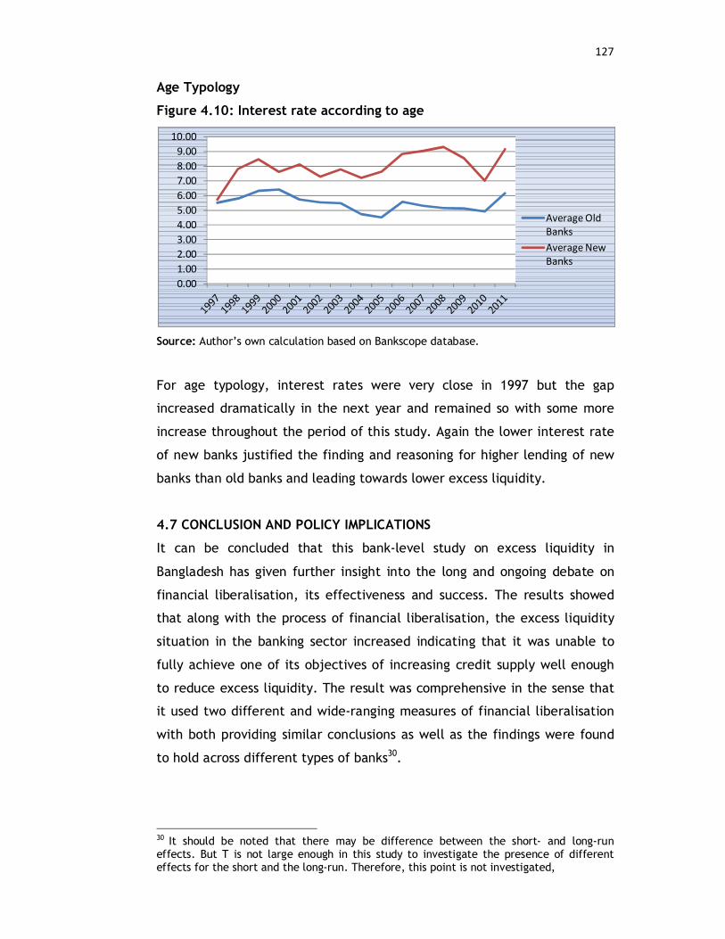
127

Age Typology

Figure 4.10: Interest rate according to age


For age typology, interest rates were very close in 1997 but the gap

increased dramatically in the next year and remained so with some more

increase throughout the period of this study. Again the lower interest rate

of new banks justified the finding and reasoning for higher lending of new

banks than old banks and leading towards lower excess liquidity.

4.7 CONCLUSION AND POLICY IMPLICATIONS

It can be concluded that this bank-level study on excess liquidity in

Bangladesh has given further insight into the long and ongoing debate on

financial liberalisation, its effectiveness and success. The results showed

that along with the process of financial liberalisation, the excess liquidity

situation in the banking sector increased indicating that it was unable to

fully achieve one of its objectives of increasing credit supply well enough

to reduce excess liquidity. The result was comprehensive in the sense that

it used two different and wide-ranging measures of financial liberalisation

with both providing similar conclusions as well as the findings were found

to hold across different types of banks30.

30 It should be noted that there may be difference between the short- and long-run effects. But T is not large enough in this study to investigate the presence of different effects for the short and the long-run. Therefore, this point is not investigated,

0.001.002.003.004.005.006.007.008.009.00

10.00

Average Old BanksAverage New Banks

128

This study allowed one to frame specific policies and its implementations

based on different bank-specific characteristics. One significant feature of

this study was that it used bank-level data which helped in understanding

better the differences at bank-level and to classify the banks according to

different typology and examine the effect accordingly.

For ownership typology, it was found that public banks had higher excess

liquidity than private banks. Therefore, it is important that public banks

step up their lending in normal times rather than using the advantage of

government backing. On the other hand, careful attention is needed so

that private banks do not lend injudiciously, which may look good in short-

run but can be detrimental in long-run due to the higher risk associated

with imprudent lending.

Similarly, for age typology, old banks were found to be having more excess

liquidity than the new banks. Hence, old banks were needed to be

encouraged to lend more using their advantages in lending towards large

firms. Since Bangladesh is a country with many small firms, old banks were

needed to concentrate in increasing their lending scope by raising lending

to small firms and consumers. Specific targets should be set for these types

of banks by the central bank in this regard as was done by the central bank

in other cases (e.g., specific targets were set for agricultural lending by

the central bank in Bangladesh). On the other hand, new banks should be

monitored so that they do not overlend, particularly during the initial years

to survive. An initial period of a few years of support may help these banks

to lend more prudently and survive in this very competitive sector.

This study observed no significant difference for mode of operation and

size typologies. These results suggested that policies should be formulated

and implemented on a priority basis where the characteristics of ownership

and age need to be addressed first. This also supported the view that ‘one

size fits all’ approach should be avoided and specific policies need to be

formulated keeping in mind different bank-specific characteristics.

129

Although bank-level variations are observed, this does not mean that

general policies are harmful and should not be taken. What this study

points out is that only general policies are not enough and tailor-made

policies for different bank characteristics based on the above findings can

be very helpful in terms of effectiveness. Therefore, a multidimensional

approach should be taken to get the maximum benefit or attainment of the

objective since these characteristics were overlapping for banks. Moreover,

special attention needs to be given for the variation in interest rates

according to bank-specific characteristics. As observed from Figures 4.8 to

4.11, rate of interest played an important role in lending and variation in

interest rates had an impact to difference in lending. Therefore, steps

need to be taken to address this variation and reduce it to a level so that

lending does not differ much according to these bank-specific

characteristics.

The financial liberalisation index constructed and applied in this study

showed that although liberalisation started in Bangladesh in the early

1990s, it was still far from reaching its completion stage. Hence, it is very

important that the remaining process is incorporated and accomplished

with urgency so that maximum benefit from it can be achieved.

Sequencing of liberalisation can also play a crucial role in achieving the

benefit from this process. If a country is at its early stage, then it is very

important to keep in mind this process of sequencing. But for countries

where the process started long back and was in place for years, it might be

useful to work on strengthening the institutional factors as a pre-requisite

for the success of financial liberalisation (Caprio et al., 2006).

130

APPENDIX 4.1: Data availability of banks in Bankscope

Table 4A.1: Data availability of banks in Bankscope

No. Name Form available Form taken

Period Total Year

1 Sonali Bank Unconsolidated U 1997-2011 15 2 Agrani Bank Unconsolidated U 1997-2011 15 3 Rupali Bank Unconsolidated U 1997-2011 15 4 Janata Bank Both (U & C) U 1997-2011 15 5 United Commercial Bank Both (U & C) U 1997-2011 15 6 Mutual Trust Bank Both (U & C) U 2000-2011 12 7 BRAC Bank Both (U & C) U 2001-2011 11 8 Eastern Bank Both (U & C) U 1997-2011 15 9 Dutch Bangla Bank Unconsolidated U 1997-2011 15 10 Dhaka Bank Limited Both (U & C) C 1997-2011 15 11 Islami Bank Bangladesh Consolidated C 1997-2011 15 12 Uttara Bank Limited Unconsolidated U 1997-2011 15 13 Pubali Bank Limited Both (U & C) U 1997-2011 15 14 IFIC Bank Limited Consolidated C 1997-2011 15 15 National Bank Limited Both (U & C) C 1997-2011 15 16 The City Bank Limited Both (U & C) U 1997-2011 15 17 NCC Bank Limited Unconsolidated U 1997-2011 15 18 Mercantile Bank Limited Unconsolidated U 1999-2011 13 19 Prime Bank Limited Both (U & C) U 1997-2011 15 20 Southeast Bank Limited Both (U & C) U 1997-2011 15 21 Al-Arafah Islami Bank Both (U & C) U 1997-2011 14* 22 Social Islami Bank Ltd Both (U & C) U 1998-2011 14 23 Standard Bank Limited Consolidated C 1999-2011 13 24 One Bank Limited Both (U & C) U 1999-2011 13 25 First Security Islami Bank Unconsolidated U 1999-2011 13 26 The Premier Bank Limited Both (U & C) U 1999-2011 13 27 Bank Asia Limited Both (U & C) U 1999-2011 13 28 Trust Bank Limited Unconsolidated U 2000-2011 12 29 Shahjalal Islami Bank Ltd Unconsolidated U 2001-2011 11 30 Jamuna Bank Limited Both (U & C) C 2001-2011 11 31 ICB Islamic Bank Limited Unconsolidated U 1997-2011 12* 32 AB Bank Both (U & C) U 1997-2011 15 33 EXIM Bank Limited Unconsolidated U 1999-2011 13

34 Bangladesh Commerce Bank Limited

Unconsolidated U 2000-2011 12

35 Bangladesh Krishi Bank Unconsolidated U 1997-2011 15

36 Bangladesh Development Bank Ltd

Unconsolidated U 1997-2009 12*

37 BASIC Bank Limited Unconsolidated U 1997-2011 15

38 Rajshahi Krishi Unnayan Bank

Not available No

* One or more year(s) missing inside the period. U = Unconsolidated, C = Consolidated

131

APPENDIX 4.2: Variable definitions

Table 4A.2: Variable definitions

Variable Name

Variable Definition

Comment

Dependent Variable

Excess liquidity Liquid assets =summing up trading securities and at fair value through income + loans and advances to banks + reverse repos and cash collateral + cash and due from banks) -mandatory reserves included above.

log value taken


Lag of excess liquidity

Lag of initial year data log value of initial year data taken

Financial liberalisation (FL)

A composite index of seven indicators following Abiad et al. but constructed by authors

Actual values taken first and then log values taken.

Deposit volatility SD of total deposit (using 3-year

overlapping SD estimation) log value taken

Deposit rate Interest expense/ average interest-bearing liabilities

log value taken

Government bills and bonds

(Treasury bill rate of 91-day) - (interest income/ average earning assets)

log value taken

Impaired loans Impaired loans / gross loans log value taken Ownership dummy with interaction

FL* Public (1 if state-owned, 0 otherwise)

Size dummy with interaction

FL* Large (1 if large, 0 otherwise)

Mode of operation dummy with interaction

FL* Islamic (1 if Islamic, 0 otherwise)

Age dummy with interaction

FL* New (1 if new {established after 1990}, 0 otherwise)

132

APPENDIX 4.3: Bank size classifications

Table 4A.3: Bank size classifications

Sl. No. Name of PCB Bank Size 1 AB Bank Small to Large 2 Agrani Bank Large 3 Al-Arafah Islami Bank Small to Large 4 Bangladesh Commerce Bank Small 5 Bangladesh Development Bank Small 6 Bangladesh Krishi Bank Small to Large 7 Bank Asia Small to Large 8 BASIC Bank Small 9 BRAC Bank Small to Large 10 City Bank Small to Large 11 Dhaka Bank Small to Large 12 Dutch Bangla Bank Small to Large 13 Eastern Bank Small to Large 14 EXIM Bank Small to Large 15 First Security Islami Bank Small to Large 16 ICB Islamic Bank Limited Small 17 IFIC Bank Small to Large 18 Islami Bank Bangladesh Small to Large 19 Jamuna Bank Small to Large 20 Janata Bank Large 21 Mercantile Bank Small to Large 22 Mutual Trust Bank Small 23 National Bank Small to Large 24 NCC Bank Small to Large 25 One Bank Small 26 Premier Bank Small 27 Prime Bank Limited Small to Large 28 Pubali Bank Small to Large 29 Rupali Bank Small to Large 30 Shahjalal Islami Bank Small to Large 31 Social Islami Bank Small to Large 32 Sonali Bank Large 33 Southeast Bank Small to Large 34 Standard Bank Small 35 Trust Bank Small 36 United Commercial Bank Small to Large 37 Uttara Bank Small to Large

Source: Defined according to total asset data from Bankscope. *Small to Large means that asset of the bank was lower than $1 billion at the beginning but crossed the threshold at some part during this period.

133

APPENDIX 4.4: Generation of PCBs in Bangladesh

Table 4A.4: Generation of PCBs in Bangladesh

Sl. No.

Name of PCB Year of Foundation/ Denationalisation*

1 Arab Bangladesh Bank Limited 1982 2 IFIC Bank Limited 1983 3 Uttara Bank Limited 1983* 4 Pubali Bank Limited 1983* 5 National Bank Limited 1983 6 Islami Bank Bangladesh Limited 1983 7 The City Bank Limited 1983 8 United Commercial Bank Limited 1983 9 ICB Islami Bank Limited 1987 10 Eastern Bank Limited 1992 11 NCC Bank Limited 1993 12 Prime Bank Limited 1995 13 Dhaka Bank Limited 1995 14 Al-Arafah Islami Bank Limited 1995 15 Southeast Bank Limited 1995 16 Social Islami Bank Ltd 1995 17 Dutch-Bangla Bank Limited 1996 18 Trust Bank Limited 1999 19 Bank Asia Limited 1999 20 EXIM Bank Limited 1999 21 First Security Islami Bank 1999 22 Mutual Trust Bank 1999 23 Mercantile Bank Limited 1999 24 ONE Bank Limited 1999 25 The Premier Bank Limited 1999 26 Standard Bank Limited 1999 27 Bangladesh Commerce Bank 1999 28 BRAC Bank Limited 2001 29 Jamuna Bank Limited 2001 30 Shahjalal Islami Bank Limited 2001

Source: Bangladesh Bank Annual Report, various issues. *Uttara Bank and Pubali Bank were denationalised to operate as private commercial bank.

134

APPENDIX 4.5: Coding rules for the financial liberalisation index Coding rules for the financial liberalisation index, in line with the work of Abiad et al. (2010), is described below. To construct an index of financial liberalisation, codes were assigned along the seven dimensions below. Each dimension had various sub-dimensions. Based on the score for each sub-dimension, each dimension received a ‘raw score.’ The explanations for each sub-dimension below indicate how to assign the raw score. After a ‘raw score’ was assigned, Abiad et al. (2010) normalised to a 0-3 scale. The normalisation was done on the basis of the classifications listed below for each dimension. That is, fully liberalised = 3; partially liberalised = 2; partially repressed = 1; fully repressed = 0. The final scores were used to compute an aggregate index for each year by assigning equal weight to each dimension. For example, if the ‘raw score’ on credit controls and reserve requirements totals 4 (by assigning a code of 2 for liberal reserve requirements, 1 for lack of directed credit and 1 for lack of subsidised directed credit), this was equivalent to the definition of fully liberalised. So, the normalisation would assign a score of 3 on the 0-3 scale. However, in this study, we avoided the normalisation process as we thought that this would reflect the process better. The questions used by Abiad et al. (2010) are described here. This study used the same seven dimensions. These seven dimensionsand the situation in Bangladesh in respect to these are given below to explain how each dimension was extended. I. Credit Controls and Reserve Requirements: 1) Were reserve requirements restrictive? Coded as 0 if reserve requirement was more than 20 per cent. Coded as 1 if reserve requirements were reduced to 10–20 per cent or

complicated regulations to set reserve requirements were simplified as a step toward reducing reserve requirements Coded as 2 if reserve requirements were less than 10 per cent.

2) Were there minimum amounts of credit that must be channeled to certain sectors? Coded as 0 if credit allocations were determined by the central bank or

mandatory credit allocations to certain sectors exist. Coded as 1 if mandatory credit allocations to certain sectors were

eliminated or do not exist. 3) Were there any credits supplied to certain sectors at subsidised rates? Coded as 0 when banks have to supply credits at subsidised rates to

certain sectors. Coded as 1 when the mandatory requirement of credit allocation at

subsidised rates was eliminated or banks do not have to supply credits at subsidised rates. II. Aggregate Credit Ceilings Coded as 0 if ceilings on expansion of bank credit were in place. This

includes bank-specific credit ceilings imposed by the central bank.

135

Coded as 1 if no restrictions exist on the expansion of bank credit. III. Interest Rate Liberalisation Deposit rates and lending rates were separately considered, in coding this measure, in order to look at the type of regulations for each set of rates. They were coded as being government set or subject to a binding ceiling (code=0), fluctuating within a band (code=1) or freely floating (code=2). The coding was based on the following description: FL=4 [2, 2] Fully Liberalised if both deposit interest rates and lending interest rates were determined at market rates. LL = 3 [2, 1] Largely Liberalised when either deposit rates or lending rates were freed but the other rates were subject to band or only a part of interest rates were determined at market rates. PR= 2/1 [2, 0] [1, 1][1, 0] Partially Repressed when either deposit rates or lending rates were freed but the other interest rates were set by government or subject to ceiling/floor; or both deposit rates and lending rates were subject to band or partially liberalised; or either deposit rates or lending rates were subject to band or partially liberalised. FR= 0 [0, 0] Fully Repressed when both deposit rates and lending rates were set by the government or subject to ceiling/floor.

IV. Banking Sector Entry The following sub-measures were considered: 1) To what extent does the government allow foreign banks to enter into a domestic market? This question was coded to examine whether a country allows the entry of foreign banks into a domestic market; whether branching restrictions of foreign banks were eased; to what degree the equity ownership of domestic banks by nonresidents was allowed. Coded as 0 when no entry of foreign banks was allowed; or tight

restrictions on the opening of new foreign banks were in place. Coded as 1 when foreign bank entry was allowed, but nonresidents must

hold less than 50 per cent equity share. Coded as 2 when the majority of share of equity ownership of domestic

banks by nonresidents was allowed; or equal treatment was ensured for both foreign banks and domestic banks; or an unlimited number of branching was allowed for foreign banks. Three questions look at policies to enhance the competition in the domestic banking market. 2) Does the government allow the entry of new domestic banks? Coded as 0 when the entry of new domestic banks was not allowed or

strictly regulated. Coded as 1 when the entry of new domestic banks or other financial

institutions was allowed into the domestic market.

136

3) Were there restrictions on branching? (0/1) Coded as 0 when branching restrictions were in place. Coded as 1 when there were no branching restrictions or if restrictions

were eased. 4) Does the government allow banks to engage in a wide range of activities? (0/1) Coded as 0 when the range of activities that bank can take consists of

only banking activities. Coded as 1 when banks were allowed to become universal banks.

The dimension of entry barriers was coded by adding the scores of these three questions. Fully Liberalised= 4 or 5, Largely Liberalised= 3, Partially Repressed= 1 or 2, Fully Repressed = 0 V. Capital Account Transactions 1) Was the exchange rate system unified? (0/1) Coded as 0 when a special exchange rate regime for either capital or

current account transactions exists. Coded as 1 when the exchange rate system was unified.

2) Does a country set restrictions on capital inflow? (0/1) Coded as 0 when significant restrictions exist on capital inflows. Coded as 1 when banks were allowed to borrow from abroad freely

without restrictions and there were no tight restrictions on other capital inflows. 3) Does a country set restrictions on capital outflow? (0/1) Coded as 0 when restrictions exist on capital outflows. Coded as 1 when capital outflows were allowed to flow freely or with

minimal approval restrictions. By adding these three items, Fully Liberalised = [3], Largely Liberalised = [2], Partially Repressed = [1], Fully Repressed= [0] VI. Privatisation Privatisation of banks was coded as follows: Fully Liberalised: if no state banks exist or state-owned banks do not consist of any significant portion of banks and/or the percentage of public bank assets was less than 10 per cent. Largely Liberalised: if most banks were privately owned and/or the percentage of public bank assets was from 10 per cent to 25 per cent. Partially Repressed: if many banks were privately owned but major banks were still state-owned and/or the percentage of public bank assets was 25 per cent to 50 per cent. Fully Repressed: if major banks were all state owned banks and/or the percentage of public bank assets was from 50 per cent to 100 per cent.

137

VII. Securities Markets 1) Has a country taken measures to develop securities markets? Coded as 0 if a securities market does not exist. Coded as 1 when a securities market was starting to form with the

introduction of auctioning of T-bills or the establishment of a security commission. Coded as 2 when further measures have been taken to develop securities

markets (tax exemptions, introduction of medium and long-term government bonds in order to build the benchmark of a yield curve, policies to develop corporate bond and equity markets, or the introduction of a primary dealer system to develop government security markets). Coded as 3 when further policy measures have been taken to develop

derivative markets or to broaden the institutional investor base by deregulating portfolio investments and pension funds, or completing the full deregulation of stock exchanges. 2) Was a country’s equity market open to foreign investors? Coded as 0 if no foreign equity ownership was allowed. Coded as 1 when foreign equity ownership was allowed but there was less

than 50 per cent foreign ownership. Coded as 2 when a majority equity share of foreign ownership was

allowed. By adding these two sub-dimensions, Fully Liberalised = [4 or 5], Largely Liberalised = [3], Partially Repressed = [1, 2], and Fully Repressed = [0] **NOTE** If information on the second sub-dimension was not available (as was the case with some low income countries), the measure was coded using information on securities market development. When information on securities markets were considered, a 0-3 scale was assigned based on the score on securities markets. VIII. Banking Sector Supervision 1) Has a country adopted a capital adequacy ratio based on the Basel standard? (0/1) Coded as 0 if the Basel risk-weighted capital adequacy ratio was not

implemented. Date of implementation was important, in terms of passing legislation to enforce the Basel requirement of 8 per cent CAR. Coded as 1 when Basel CAR was in force. (Note: If the large majority of

banks meet the prudential requirement of an 8 per cent risk-weighted capital adequacy ratio, but this was not a mandatory ratio as in Basel, the measure was still classified as 1). Prior to 1993, when the Basel regulations were not in place internationally, this measure takes the value of 0.

2) Was the banking supervisory agency independent from executives’ influence? (0/1/2) A banking supervisory agency’s independence was ensured when the banking supervisory agency can resolve banks’ problems without delays.

138

Delays were often caused by the lack of autonomy of the banking supervisory agency, which was caused by political interference. For example, when the banking supervisory agency has to obtain approval from different agencies such as the Ministry of Finance (MOF) in revoking or suspending licenses of banks or liquidating banks’ assets, or when the ultimate jurisdiction of the banking supervisory agency was the MOF, it often causes delays in resolving banking problems. In addition to the independence from political interference, the banking supervisory agency also has to be given enough power to resolve banks’ problems promptly. Coded as 0 when the banking supervisory agency does not have an

adequate legal framework to promptly intervene in banks’ activities; and/or when there was the lack of legal framework for the independence of the supervisory agency such as the appointment and removal of the head of the banking supervisory agency; or the ultimate jurisdiction of the banking supervision was under the MOF; or when a frequent turnover of the head of the supervisory agency was experienced. Coded as 1 when the objective supervisory agency was clearly defined

and an adequate legal framework to resolve banking problems was provided (the revocation and the suspension of authorisation of banks, liquidation of banks and the removal of banks’ executives etc.) but potential problems remain concerning the independence of the banking supervisory agency (for example, when the MOF may intervene into the banking supervision in such as case that the board of the banking supervisory agency board was chaired by the MOF, although the fixed term of the board was ensured by law); or although clear legal objectives and legal independence were observed, the adequate legal framework for resolving problems was not well articulated. Coded as 2 when a legal framework for the objectives and the resolution

of troubled banks was set up and if the banking supervisory agency was legally independent from the executive branch and actually not interfered with by the executive branch. 3) Does a banking supervisory agency conduct effective supervisions through on-site and off-site examinations? (0/1/2) Conducting on-site and off-site examinations of banks was an important way to monitor banks’ balance sheets. Coded as 0 when a country has no legal framework and practices of on-

site and off-site examinations was not provided or when no on-site and off-site examinations were conducted. Coded as 1 when the legal framework of on-site and off-site examinations

was set up and the banking supervision agency have conducted examinations but in an ineffective or insufficient manner. Coded as 2 when the banking supervisory agency conducts effective and

sophisticated examinations. 4) Does a country’s banking supervisory agency cover all financial institutions without exception? (0/1) If some kinds of banks were not exclusively supervised by the banking supervisory agency or if offshore intermediaries of banks were excluded from the supervision, the effectiveness of the banking supervision was seriously undermined.

139

Coded as 1 when all banks were under supervision by supervisory agencies without exception. Coded as 0 if some kinds of financial institutions were not exclusively

supervised by the banking supervisory or were excluded from banking supervisory agency oversights. Enhancement of banking supervision over the banking sector was coded by summing up these four dimensions, which were assigned a degree of reform as follows. Highly Regulated = [6], Largely Regulated = [4-5], Less Regulated = [2-3], Not Regulated = [0-1]

140

Appendix 4.6: Coverage area of this study of the banking sector During the period of this study (1997-2011), there were altogether 47 banks operating in Bangladesh. Of them, 9 were foreign commercial banks. As mentioned in footnote 4, they were excluded due to data unavailability. For the same reason, one specialised bank, Rajshahi Krishi Unnayan Bank, could not be included in this study. With the exception of these 10 banks, all the remaining banks were included in this study. These 37 banks included in the study, represent the banking sector in Bangladesh very well since they account for more than 99 per cent of bank branches. Moreover, they had a share of more than 90 per cent of assets and deposits of these 47 banks (Bangladesh Bank Annual Report, 2013). These are graphically presented here with the help of table and pie charts. Table 4A.5: Coverage area of this study of the banking sector in 2011 Classification Number of

branches Total assets

(in billion taka) Deposits

(in billion taka) Share of banks excluding FCBs

7898 5482.2 4237.5

Share of FCBs 63 385.4 272.2 TOTAL 7961 5867.6 4509.7

Source: Bangladesh Bank Annual Report 2013. Figures 4A.1: Coverage area of this study of the banking sector

Share of banks excluding FCBs

99%

Share of

FCBs1%

Number of branches (in per cent)

141

It may be mentioned that recently in 2012, ten more new banks were established. But they were not included in this study as they were established after the study period.


93%

Share of

FCBs7%

Total assets (in billion taka) in per cent


94%

Share of

FCBs6%

Deposits (in billion taka) in per cent

142

CHAPTER 5 EXCESS LIQUIDITY ACCORDING TO BANK TYPOLOGY, BUSINESS

CYCLE AND THE FINANCIAL CRISIS

5.1 INTRODUCTION

There were many studies on the lending behaviour with different bank

ownerships in terms of business cycle. It was observed that different types

of banks had different lending patterns over the business cycle. Some of

them were procyclical, some were counter-cyclical while some were

acyclical. These studies were generally done for public and private banks.

Although it was not true in all cases but generally it was observed that

private banks’ lending pattern was procyclical whereas public banks lent

less procyclically in most cases (Davydov, 2013). However, sometimes the

lending of public banks was found to be even counter-cyclical (Bertay et

al., 2012). Some other studies found mixed results for different countries

or regions (Cull and Peria, 2012) while some others did not find any

significant difference in lending between these two types of banks

(Iannotta, et al., 2011).

Another interesting and related topic which may also affect the lending

behavior of banks was crisis time. Generally it was observed that public

banks were less procyclical than the private banks in non-crisis times.

During the recent financial crisis of 2008-09, the public banks played a

positive role for the economy by either acting counter-cyclically or at least

less procyclically.

In some cross-country studies on non-crisis times, it was commonly found

that public banks were less efficient, and sometimes led to lower financial

development, than the private banks (Barth et al., 2004; Bonin et al.,

2005; Duprey, 2013). Micco et al. (2007) observed that this feature of

higher efficiency of private banks was truer for developing countries than

the developed countries. However, since public banks had additional

143

agenda to fulfill, this property of efficiency might not be appropriate to

distinguish between public and private banks.

This view of dissimilarity in lending according to ownership was also

supported by various country-level studies. For example, Berger et al.

(2008) observed it for Argentina, Lin and Zhang (2009) found it for China,

and Omran (2007) witnessed it for Egypt. But in some cases it was observed

that public banks and private banks were almost equally efficient (Beck et

al., 2005; Kraft et al., 2006).

Since most of the earlier studies discussed the differences in ownership and

their effect, this study addressed the issue using some additional typologies

of banking. This included the most common typology of ownership (public

versus private banks) along with size (small versus large banks), mode of

operation (Islamic versus conventional banks) and age (new versus old

banks). It would be interesting to see if the large banks behaved differently

from the small banks about their liquid assets while if there was any

pattern for new banks which separated them from the old banks. The

growth of Islamic banking worldwide and in Bangladesh made it a very

worthy effort to investigate if they differed from the conventional banks.

5.1.1 Capitalisation and Excess Liquidity

After the financial crisis of 2007, a process of recapitalisation started to

help the banking sector. The Euro area governments announced different

measures to support these institutions and one of them was recapitalisation

of the financial institutions in difficulty (Stark, 2009). This phenomenon

was also observed by Brei and Gadanecz (2012), especially for the G10

countries. In another paper, the authors mentioned that public

recapitalisations were almost equal to $500 billions between 2007 and 2010

(Brei et al., 2013) in the G10 countries. Brei and Gadanecz (2012) observed

that majority funds were provided during the period of 2008Q4 to 2009Q1

and most funds were allocated to US, UK, Germany, Netherlands and

France.

144

Therefore, it was important to see if the process of capitalisation was

related with excess liquidity. Delechat et al. (2012), in their study of 96

commercial banks from Central American countries, observed that there

was significant inverse relationship between capitalisation and excess

liquidity. According to them, better capitalised banks had easier access to

markets and thus held less liquidity.

Capitalisation could play a key role in reducing the liquidity risk of the

banks which in turn could reduce the amount of excess liquidity any bank

holds. Since the amount of capitalisation could vary according to bank

typologies, it was important to examine how different bank types were

affected and how they differed in keeping excess liquidity. For example,

public banks have the government to back up in case of any emergency and

hence they will be less worried about the liquidity risk and may end up

keeping less excess liquidity than the private banks. Similarly, large banks

would be more capitalised than the smaller ones and therefore small banks

would keep more excess liquidity than large banks due to the higher

liquidity risk.

Walker (2012) found evidence that the lending behaviour of less well-

capitalised banks was more sensitive to monetary policy shocks than that of

better-capitalised banks. Opolot (2013) observed that the interaction term

between bank capitalisation and monetary policy was positive and

significant implying that banks with high capitalisation ratio were able to

offer more loans during a period of monetary policy 31 tightening (also

supported by Zulkefly et al., 2010). This could be due to the fact that

banks with higher capitalisation ratio might not be affected that much by a

contractionary monetary policy stance.

5.1.2 Structural and Cyclical Factors

Based on the characteristics, the determinants of the involuntary excess

liquidity could be classified into two types: (i) structural factors – due to 31 Monetary policy is one of the policies of central bank involving management of money supply mainly using interest rate with the objectives include attaining growth, low unemployment and controlling inflation.

145

macroeconomic and financial development – and (ii) cyclical factors

(Pontes and Murta, 2012). The first structural determinant of involuntary

liquidity was low degree of financial development. This was inversely

related with excess liquidity since an inefficient interbank market and high

costs of financial operations (e.g. evaluation and monitoring costs) lead

banks to keep higher level of reserves (Agenor and Aynaoui, 2010). High

degree of risk aversion was another structural determinant. It was

positively related with excess liquidity as it caused banks to demand a high

risk premium and lowered private sector credit demand. The degree of risk

aversion was related with macroeconomic instability (Agenor and Aynaoui,

2010). Other structural factors included asymmetric information and lack

of competition in the banking sector (Saxegaard, 2006).

Among the cyclical factors, inflation was the most mentioned one. This

was positively related as a rise in inflation caused higher volatility in

relative prices and higher uncertainty in the risk degree of investment

projects and in the value of collateral (Agenor and Aynaoui, 2010).

Therefore, leading banks to demand higher interest rates on loans which

reduced the credit demand and thereby increasing excess liquidity.

Another cyclical determinant was capital inflow. This could happen as a

result of various reasons which include oil commerce receipts, foreign

direct investment (FDI) associated with liberalisation of capital flows

and/or foreign aid (Saxegaard, 2006). It was also observed that steps

removing restrictions on capital inflows for non-residents (maintaining the

restrictions on capital outflows), along with privatisation of state

enterprises could lead to large inflows of capital intermediated by banks

and hence to larger amount of excess liquidity (Agenor and Aynaoui, 2010).

5.1.3 Contribution of this Chapter

The objective of this research was to fill some of the gaps in this strand of

literature. The main questions addressed in this study are described below.

(i) Does ownership matter in case of the effect of business cycle? From

earlier studies, it could be observed that public banks may had less excess

146

liquidity due to the fact that these banks had support from the government

and therefore would worry less than the private banks about the liquidity

risk. We would like to test if business cycle affects the excess liquidity

situation differently between public and private banks.

(ii) Does the effect of business cycle vary with bank size? This study

examined if business cycle affected differently the excess liquidity

situation for large and small banks. From the point of capitalisation, it was

mentioned that large banks were more capitalised and therefore would

have less excess liquidity than the small banks due to fear of liquidity risk.

(iii) Was there any difference according to age? Another issue was to look

at whether old banks have more or less excess liquidity than new banks.

For newer banks, it was easier to raise deposits and relatively difficult to

identify reliable borrowers. Hence, it was expected that new banks would

have more excess liquidity than old banks since the old banks usually have

more information and it becomes easier for them to screen the borrowers.

(iv) Were Islamic banks affected differently? Since Bangladesh is a Muslim

populated country and the Islamic banking system was flourishing quickly

and formed a substantial part, therefore it was important to see if the

Islamic banking system was affected differently in terms of excess liquidity

situation from the conventional banking system. It was generally observed

that Islamic banks, due to its inherent restrictions, did not have enough

instruments like the conventional banks to address the issue of excess

liquidity and therefore suffered more from this problem. So, it was

expected that Islamic banks will have more excess liquidity than the

conventional banks.

(v) Were financial crisis and excess liquidity related? Financial crisis is a

time when the banks would not feel very confident to lend and there would

be less demand from the investors’ side. Hence there was supposed to be a

positive relationship between the crisis and the excess liquidity. However,

the period of crisis was normally accompanied by a process of

147

recapitalisation to make the economy move on by increased lending. This

process might in turn reduce the amount of excess liquidity. Therefore,

excess liquidity is expected to increase in the short-term and decrease

later.

(vi) Did the relationship of excess liquidity with financial crisis follow

the same pattern as business cycle? Finally this study also saw if the

relationship of different bank typologies (ownership, size, mode of

operation and age) followed the same pattern of relationship as it did for

the business cycle bust or did it follow a different pattern. It would be

interesting to see if all these typologies had a significant impact on excess

liquidity with the process of business cycle or in time of the financial crisis.

It could happen that in some cases, they were significant while in some

other cases, they were not. This indicated differences of the impact on

these typologies.

5.2 PREVIOUS WORKS

Most of the studies in this area were cross-country studies. As discussed in

Section 5.1, the general finding was that public banks lend less

procyclically in most cases. While sometimes the lending was found to be

counter-cyclical, some studies also found mixed results for different

countries or regions and some did not find any significant difference.

Similarly, different ownerships of banks had different lending patterns

during the crisis time. In different cross-country studies on non-crisis times,

it was commonly found that public banks were less efficient and sometimes

led to lower financial development than the private banks. This feature of

higher efficiency of private banks was truer for developing countries than

the developed countries.

Davydov (2013) identified three possible reasons for the comparative

inefficiency of the public banks. These were: (i) political interference, that

deviate them from the profit maximisation aims; (ii) incentives structure

for managers were weaker than the private banks; and (iii) inferior

incentives for owners leading to poor monitoring.

148

However, as already mentioned, comparing public and private banks in

terms of efficiency or profitability can be misleading (UNCTAD, 2008) since

public banks have other agenda (along with that of profitability) and hence

pursuing solely the profit objective is not their aim. Therefore, they may

sometime need to sacrifice the objective of profit maximisation and

become less profitable than the private banks. This (less profitability) does

not imply that the public banks were less efficient.

During the recent financial crisis of 2008-09, public banks played a positive

role for the economy by generally acting counter-cyclically (Allen et al.,

2013) or less procyclically (Fungacova et al., 2013). This was crucial and

helped the economy to stabilise as the domestic private banks acted

procyclically (Kowalewski and Rybinski, 2011; Cull and Peria, 2012). This

was also true for earlier financial crises in Asia and Latin America in the

1990s (Hawkins and Mihaljek, 2001).

Micco and Panizza (2006), in their study of 179 countries, mentioned four

possible reasons why public banks stabilise credit. These were:

(i) it was part of their objectives as public banks;

(ii) generally it was considered by depositors to be a safer place during

possible bank failures, hence the public banks end up having a

better deposit base during the crisis and thereby also in a better

position to smooth credit;

(iii) sometimes the public banks do not have a proper set of incentives

and hence the public bank managers can be lazy;

(iv) politicians might try to influence public bank lending in election

years.

Bank lending and excess liquidity were very closely related two aspects

(Alper et al., 2012) of the banking sector and there were many works on

lending and bank ownership related to the financial crisis and business

cycle. Interestingly enough, there were very few empirical works on excess

liquidity directly related to the financial crisis, especially investigating the

aftermath of the crisis on excess liquidity. Similar was also true for

149

business cycle and excess liquidity. Therefore, this study is trying to fill this

gap in the existing literature with the following three objectives. Firstly, by

investigating how excess liquidity was affected when the recent financial

crisis occurred. Secondly, to see the movement of excess liquidity with the

business cycle process. Finally, examine if there were any differences in

excess liquidity situation in terms of ownership, size, mode of operation

and age.

The boom and bust of the business cycle can have an effect on the excess

liquidity situation of the banks. During economic boom, there is an increase

in demand for loans and the probability of loan default decreases. This

makes banks become softer in lending which may reduce the excess

liquidity situation. During the bust or downturn, banks become stricter as

the probability of loan default increases. Moreover, investors also become

more careful in investing at this time and may deposit more in banks. This

implies that the relationship between the business cycle and the excess

liquidity is generally expected to be negative meaning that during the

boom period of the business cycle, there will be less excess liquidity while

during the bust period, the excess liquidity will be more (Ruckes, 2004).

Therefore, an inverse relationship is expected to prevail between business

cycle and the excess liquidity.

The financial crisis and business cycle can be closely related due to the

fact that if the downturn or recession of the business cycle goes on for a

long time, it can lead to crisis. This reasoning was supported by Bordo et

al. (2001): “crises are an intrinsic part of the business cycle and result from

shocks to economic fundamentals.”

Heeboll-Christensen (2011) used the US data from 1987 to 2010 and found

that “mechanisms of credit growth and excess liquidity are found to be

closely related.” According to this study, housing bubble was created

initially with a prolonged credit cycle and was fuelled by excess liquidity

and led to the financial crisis of 2007.

150

The existing works on financial crisis and excess liquidity can broadly be

divided into two categories. One group discussed how excess liquidity acted

as one of the factors for the financial crisis (Palma, 2009; Acharya and

Naqvi, 2012; Brana et al., 2012).

The other group discussed how the crisis situation could affect excess

liquidity. One of the possible effects of financial crisis was that it increased

the uncertainty and riskiness in the economy. This made lending riskier for

the banks. Therefore, banks lend less and thereby increasing the excess

liquidity situation. This was found in the studies of Agenor et al. (2004) for

Thailand and Ashcraft et al. (2011) for US. Montoro and Moreno (2011)

found similar results for Peru. In another study, Murta and Garcia (2010)

examined the excess liquidity in the banks of the Euro area.

The most direct empirical study till now, to our knowledge, that examined

the effect of the recent financial crisis on the excess liquidity situation of

the banking sector was carried out by Pontes and Murta (2012). They

studied this relationship for the African economy of Cape Verde. Their

results suggested that the crisis decreased the excess liquidity in the

economy. The possible reasons included the extreme dependence of the

economy on the external economic factors (especially remittance) and also

the underdevelopment of the financial markets.

5.3 THE FINANCIAL CRISIS AND THE BANGLADESH ECONOMY

The experience of the recent financial crisis showed that not all economies

were affected at the same time. Some were affected immediately (termed

as first shockwave), some were after some time (called second shockwave

through impact on credit), while some were after even some more time

(named third shockwave through impact on real economy). Like other

economies, the global financial crisis of 2007 also affected the economy of

Bangladesh. However, it did not impact the economy immediately but after

some time. According to Rahman et al. (2009), the crisis started affecting

the economy of Bangladesh from October 2008. One of the main features of

151

this crisis was that “the crisis has evolved from financial crisis to credit

contraction to crisis of confidence.”

The lag effect of crisis could be due to the very little exposure of the

capital market in Bangladesh to the foreign portfolio investment (only

2.4%). This perhaps led Bangladesh to survive the first shockwave.

However, it started to feel the impact from the second shockwave. The

economy was mainly affected through the three channels of exports,

remittances and foreign investment.

One of the key factors of the impact of these channels depended on the

economic performance of the main partner countries (Murshid et al.,

2009). As they were unable to perform well, the crisis also affected the

Bangladesh economy negatively.

Ali and Islam (2010) stated that although the financial crisis did not affect

the economy very harshly but it still slowed down along with exports and

remittances. However, they also mentioned that Bangladesh performed

well in agriculture and in equity markets to counterbalance the effect of

the financial crisis. Raihan (2010) also mentioned that the crisis affected

the export sector negatively and some categories had to suffer negative

growth both in terms of value and volume.

5.4 EMPIRICAL APPROACH

There were various works on the relationship between bank lending and

ownership during business cycles. Recently the focus shifted to examine

the lending pattern of different types of banks during and after the crisis.

The main reason for this shift of focus of the recent works was mainly due

to the ‘Great Recession’ that occurred from 2007. Because of this, it

became important to investigate how it affected the excess liquidity

situation of banks and recently the focus shifted to address this issue to

some extent (Micco et al., 2007; Omran 2007; Lin and Zhang, 2009;

Davydov, 2013; Duprey, 2013).

152

However, these studies mainly examined the effect of ownership of banks

to see the effect of lending. But our study goes further to see other

possible and pertinent bank-specific characteristics and their impact on

excess liquidity via lending. According to our knowledge, the four bank-

specific characteristics used in this study had not been used previously

together to study excess liquidity. This was done to have a very

comprehensive picture of how bank typologies affect the excess liquidity

pattern in the banks.

While many works have already been done on the lending pattern of

banking sector and also between different types of banks, they were mostly

cross-country studies. Furthermore, the studies (especially the empirical

ones) on the relationship between excess liquidity and banking sector and

its types were very sparse. As mentioned earlier that lending and excess

liquidity were related (and since this work was on the excess liquidity),

therefore it would be pertinent to look into how the excess liquidity

situation of different types of banks varied with the business cycle and also

with the financial crisis.


From the earlier studies, it was generally observed that during economic

recession or crisis, there would be more excess liquidity and there would

be generally an inverse relationship between excess liquidity and the

business cycle. This relationship would be similar in times of crisis also.

However, different typologies based on bank-specific characteristics might

not be related in the same way and for each classification, there could be

variation in the direction, degree and significance of the relationship

(discussed in detail in sections 4.3.3 and 5.1.3). To investigate this

relationship, excess liquidity would be the dependent variable to see how

it was affected by different typologies of banking. Additionally, business

cycle and the financial crisis were also included in the analysis to see their

relationship with excess liquidity.

153

The data was collected from Bankscope. The excess liquidity was

calculated by summing up: trading securities and at fair value through

income, loans and advances to banks, reverse repos and cash collateral and

cash and due from banks. Then mandatory reserves included above were

deducted. As there were banks of different sizes according to assets,

therefore growth rate of liquid assets was taken to proxy for the excess

liquidity to avoid the scale problem. Logarithm values of these were taken

first and then growth rate was calculated by deducting the log value of the

previous year. Hence, one observation was lost per series.


5.4.2.1 Standard Control Variables from Earlier Studies on Lending and

Excess Liquidity

Different explanatory variables were used in the studies of lending. Of

them, some variables may also impact the excess liquidity. These include:

capital, size, age, economic growth and inflation rate. Of these, the first

three were bank-specific variables while the last two were macroeconomic.

Among the macroeconomic variables, a measure similar to GDP growth has

been used to empirically emulate the business cycle. Therefore, this

variable was not included.

Different studies captured the effect of macroeconomic variables. Among

the cross-country studies, Allen et al. (2013) employed GDP growth and

inflation rate to capture the effect of the macroeconomic variables.

GDP growth rate: GDP growth rate was used extensively in different works

to see the effect of macroeconomic variables (Micco et al., 2007; Bertay et

al., 2012; Allen et al., 2013). There could be two possible effects of

economic growth on excess liquidity. On one hand, economic growth would

continuously increase the lending opportunities of the banks and reduce

excess liquidity. On the other hand, there would be higher demand for

deposits with the improvement in the overall economic condition of the

people, making banks cautious to keep enough deposits which might lead

to higher excess liquidity.

154

In their study on 111 countries, Bertay et al. (2012) used constant per

capita GDP. In an even bigger study of 179 countries, Micco et al. (2007)

used the GDP growth rate. Following Micco et al. (2007), GDP growth rate

was used in this study.

Inflation: Inflation could also possibly play a role in excess liquidity

situation of the banks. This relationship and the logic were very similar to

that of economic growth.There could be two possible effects of inflation on

excess liquidity. On one hand, inflation would continuously increase the

demand for loans of the banks which would reduce excess liquidity. On the

other hand, there would be higher demand for deposits due to devaluation

of money because of inflation, forcing banks to keep more deposits which

may led to higher excess liquidity.

Among the country-specific studies, Akinboade and Makina (2010) used

inflation as one of the variables in their study on South Africa. Bertay et al.

(2012), in their study on 111 countries, measured inflation as the

percentage change in the GDP deflator and used the World Development

Indicators database of 2011. Bhaumik et al. (2011) used industry growth in

their study on India as for that particular scenario, which was more

relevant than the GDP growth (Bhaumik and Piesse, 2008). They also used

inflation but found insignificant result32.

Reserve requirement: Earlier studies on excess liquidity used various

factors as the determinants of excess liquidity. One of the most important

variables of excess liquidity that emerged from the previous studies was

reserve requirement. With the same amount of deposit available, if the

reserve requirement was higher in the banking sector then it was expected

that there would be lower excess liquidity while lower reserve requirement

(assuming the same amount of deposit) would mean banks have higher

excess liquidity. Therefore, reserve requirement was expected to have

negative relationship with the dependent variable.

32Our observation was also similar in preliminary estimation. Therefore, inflation was not included in the final regression.

155

In their study on Thailand, Agenor et al. (2004) included it as one of the

explanatory variables and found it to be significant. Aikaeli (2011) also

studied the excess liquidity problem for Tanzania and found that along with

other variables, the rate of required reserves was also responsible for

accumulation of excess liquidity in commercial banks in Tanzania. One

point that needs to be noted was that the inclusion (and significance) of

this variable depends on how excess liquidity was measured. If, as many

studies had done before, excess liquidity was proxied by bank liquidity then

reserve requirements should be included as an explanatory variable. If,

however, excess liquidity was measured net of required reserves then it

should not be included as an explanatory variable. Since this study used the

second type of definition of excess liquidity, therefore this variable was not

included in the final regression.

Period of stress: There was also an indication in the literature that excess

liquidity might vary during periods of stress relative to normal situations,

leading to greater asset price volatility during the former and so disrupting

liquidity targets (Cohen and Shin, 2003). Morrison (1966) did a study on

banks’ demand for excess reserves in both banks’ panic and non-panic

periods. He concluded that excess reserves were held as a buffer to avoid

asset transaction costs emanating from unforeseen and transitory deposit

shocks. This sort of excess liquidity could also be interpreted as an

insurance against deposit outflows. Al-Hamidy (2013) found that turbulent

international markets slowed down domestic credit growth and increased

excess liquidityfor the economy of Saudi Arabia.

Political motive: One possible reason for changes in excess liquidity

situation in the banking sector was the political situation. Fielding and

Shortland (2005) estimated a time-series model of excess liquidity for the

Egyptian banking sector and observed that political instability increased

excess liquidity while Micco et al. (2007) found that political consideration

played a role in lending differences according to bank ownership. This view

was also found by others like Cole (2009) for India, Khwaja and Mian (2005)

for Pakistan, Carvalho (2010) for Brazil, Sapienza (2004) for Italy, and Dinc

156

(2005) for a cross-country study. Normally dummy variables for election

years were used to see this relationship. For example, Micco et al. (2007)

used a dummy variable for election that was equal to 1 when the country

was in election year and zero otherwise.

The main reason for this was that sometimes election years had a

significant impact on bank lending (Dinc, 2005) due to the pressure from

politicians during that time to win the elections. Khwaja and Mian (2005)

also found political influence as an important factor for lending by public

banks in Pakistan. However, this was not true for all cases as Chen and Liu

(2013) found that lending of public banks do not change during the election

years and private banks lend more during election years in Taiwan.

An interesting term has been used by Bhattacharya (The News Today, 2013)

which ascertains that election years can be related with the business cycle.

According to him:

“Ahead of the election, the country enters into a ‘political

business cycle (PBC)’. So, both the opposition and ruling

leaderships need to deal with the matter so that country’s

economy does not experience any shock.”

Hence, it was important to see if political motive played any role in the

excess liquidity situation. As election years were mainly used to see if and

how the political motive plays any role, therefore dummy was used here

for this variable where the value was 1 for election years and 0 otherwise.

The value of 1 was only assigned when the full parliamentary elections

were held33.

5.4.2.2 Key Variables of Interest

The main variables of interest in this study were business cycle and the

financial crisis. Bank typology variables were also included to see if there

was any pattern among different types of banks in terms of excess liquidity 33 This is in line with the work of Chen and Liu (2013) where the value of 1 was given only when the Presidential elections took place.

157

due to business cycle and the financial crisis. The main objective was to

see whether different types of banks vary in their excess liquidity situation

in relation to business cycle and the financial crisis. It could shed important

light if it was known that any particular type of banking has procyclical,

counter-cyclical or acyclical relationship with business cycle and the

financial crisis.

Some of the standard variables in the literature were also incorporated to

see the direction and significance of their relationship. Measurement of

these determinants in the context of bank-level study of excess liquidity

was also discussed.

Business cycle: Among the explanatory variables, the main variable of

interest was the business cycle. Business cycle could be defined and

identified as showing high and low economic growth in an economy. While

the boom period of the business cycle could lead to higher loan demand, it

was expected that there will be less excess liquidity in the banks. However,

banks would also need to keep higher amount of deposits to meet the

demand of the customers who were expected to spend more during the

boom periods.

It could be measured in many ways but the most conventional method of

measuring it was through the GDP growth rate (Micco and Panizza, 2006). It

was observed that GDP growth at both aggregate (Duprey, 2013) or at

individual level (i.e. GDP per capita growth rate), was used for this purpose

(Bertay et al., 2012). While the first one was more relevant to see how the

expansion of GDP affected the relevant variable, the latter one was more

related with the development issues. Among these two, the more

conventional way of estimating business cycle was by measuring with the

GDP growth rate. However, there were many other sophisticated methods34

to calculate it and one of the most common one was the Hodrick-Prescott

(HP) method, proposed by Hodrick and Prescott (1997). Because of its many

34 These include the Phase-Average Trend (PAT) method, the Christiano-Fitzgerald (CF) filter, the Baxter-King (BK) filter and the Multivariate Direct Filter Approach (MDFA).

158

advantages, the HP filter was used in this study. The advantages include its

flexibility and its ability to calculate by minimising the gap between the

actual and trend output and the trend output rate change. Another major

advantage of the HP filter was that it can be applied even when the data

was nonstationary.

The HP filtered output trend and the output gap between actual and

potential GDP was also used (Duprey, 2013). This variable, defined as

‘MacroShock’ by Duprey (2013), was used in both absolute and interaction

form. Akinboade and Makina (2010) used coincidental indicators to

represent the business cycle. The index of coincidental indicators35 was a

combination of different business cycle indicators which moved along with

the economy and hence a positive value indicates higher economic growth

and vice versa.

Stolz and Wedow (2005) used different measures to calculate business

cycle fluctuations in their study on Germany. These included: i) the real

GDP growth rate; ii) the real GDP growth rates by state (SGDP); and iii) the

real output gap (measured by subtracting a non-linear trend from real GDP

using the HP filter).

As mentioned before, the HP method was proposed by Hodrick and Prescott

in 1997 (although their original work appeared in the form of a working

paper in 1980). One major advantage of it was that it may be applied when

the data was nonstationary. This removed a major problem which was

faced by researchers when macroeconomic or financial data were used

(Baum, 2006). It was also flexible and was able to calculate by minimising

the gap between the actual and trend output and the trend output rate

35Coincidental indicators are indicators of the state the economy is in at the present, including: number of employees outside of the agriculture sector, personal income less transfer payments, industrial production and manufacturing and trade sales. These indicators occur at approximately the same time as the conditions they signify. Rather than predicting future events, coincidental indicators change at the same time as the economy. For instance, personal income is a coincidental indicator for the economy: high personal income rates will coincide with a strong economy.

159

change. For these advantages, the HP filter was still used extensively

(Woitek, 1998; Gyomai and Wildi, 2013).

The HP filter was an algorithm that “smoothes” the original time series

to estimate its trend component . The cyclical component was the

difference between the original series and its trend, i.e.,

= + (5.1)

Where was constructed to minimise:

T T

tttttty1

1

2

211

2 )]()[()(

The first term was the sum of the squared deviations of from the trend

and the second term, which was the sum of squared second differences in

the trend, was a penalty for changes in the trend’s growth rate. The larger

the value of the positive parameter , the greater the penalty and the

smoother the resulting trend will be. If, e.g., = 0 , then = , =

1, … , . If → ∞, then was the linear trend obtained by fitting to a

linear trend model by OLS.

For quarterly data, Hodrick and Prescott suggested a value of q = 1/1600.

This value was used and referred to as a smoothing constant. For annual

data, Harvey and Trimbur (2008) commented that a smoothing constant

value of 6.25 for annual data would be equivalent to 1600 for quarterly

data. This smoothing parameter of 6.25 for annual data has been applied

by researchers (e.g. Duprey, 2013; Ravn and Uhlig, 2002) and was also

applied in this study to estimate the business cycle for Bangladesh.

Although the HP filter still remained a very popular method, there were

many other filters. Among these other measures of detrending and

calculating the business cycle, the most prominent ones include the PAT

method, the CF filter and the BK filter. The PAT method was used in

combination with the Bry-Boschan turning point detection algorithm. The

160

resulting medium-term cycle was smoothed by the Months for Cyclical

Dominance (MCD) method to yield the final smooth cycle. Baxter and King

(1995) constructed the BK filter which was a bandpass filter of finite order

K which was optimal in the sense that it was an approximate bandpass

filter with trend-reducing properties and symmetric weights which ensure

that there was no phase shift in the filter output. The CF random walk

filter was a band pass filter that was built on the same principles as the BK

filter. These filters formulate the de-trending and smoothing problem in

the frequency domain.

Harding and Pagan (2005) stated that cycles can be measured in three main

ways: i) classical (or business) cycles that were measured by the

fluctuations in the level of an economic variable; ii) deviation cycles that

were measured by the differences between the level and permanent

component of an economic variable; and iii) growth rate cycles that were

measured by the growth rates of level variables. Egert and Sutherland

(2012) observed that HP method was a good way to determine the business

cycle.36 As mentioned earlier, one major advantage of the HP filter was

that it could be used even if the data was nonstationary which removed a

major problem generally faced when macroeconomic or financial data were

used. Therefore, HP filter was used in this study to derive the business

cycle for Bangladesh. The HP trend value of log of GDP was estimated first

and then the difference was taken from the actual value to identify the

business cycle.

Financial crisis: There were very few empirical works on the relationship

between excess liquidity and the financial crisis. One of the determinants

of the excess liquidity studies in general, the deposit volatility, was

included in these works (Pontes and Murta, 2012). This was measured by

Pontes and Murta (2012) for Cape Verde as the moving average of the

standard deviation of private sector deposits divided by the moving average

of the same variable. Fadare (2011) examined the banking sector liquidity

36 The cycle can also be measured by the growth rate of customer loans, by GDP growth, and by the growth rate of house and share prices (Egert and Sutherland, 2012).

161

for the economy of Nigeria to see the effect of the financial crisis. A

different approach was taken by him where the basis was to see if the

actual loan-to-deposit ratio was above or below the predicted value. If the

actual value was above the predicted value, then it implied less liquid

assets while less actual value than the predicted value meant more liquid

assets. This approach reflected the comment made by Moore (2009):

“If the actual loan-to-deposit ratio is above the predicted value

this would suggest that commercial banks were less liquid than is

consistent with fundamentals, while if the actual ratio is below

the predicted value commercial banks were more liquid than

what is consistent with economic fundamentals.”

This approach was applied for the specific years of the financial crisis (i.e.

2007-09) and was found that during the financial crisis, the banks in Nigeria

became much less liquid and hence more vulnerable to the crisis although

in normal or non-crisis times, the banks were normally holding excess

liquidity.

The possible final effect of the financial crisis was also ambiguous since it

was expected that initially there would be higher excess liquidity in the

banks due to lower demand and higher risk. However, as governments and

other organisations recapitalise the banking sector during these periods to

boost the economy, banks would be able to lend more and thereby reduce

excess liquidity situation. Again, there can be higher excess liquidity if

banks lend less than they were recapitalised.

Like the business cycle variable, the financial crisis variable can also be

used in both absolute and interaction terms. They were generally given

value of 1 for the crisis dummies in years 2008 and 2009 and 0 for others.

The interactions of crisis and public bank dummies can show how public

banks performed in this period relative to private banks. Dummy variable

for crisis was also used by Allen et al. (2013). Kapan and Minoiu (2013)

divided the sample period into ‘before’, ‘shock’ and ‘after’ period where

the shock period was from July 2007 to September 2008, which was the

162

period of US subprime crisis. Davydov (2013) used crisis dummy variable

that equals one in fiscal years 2008, 2009 and 2010.

Although the financial crisis started in September 2007, the effect of it

reached Bangladesh in 2008 and the effect continued in the following year.

Therefore, 2008 and 2009 were the most appropriate years and were given

value of 1 during these two years. The interactions of crisis and bank

typology dummies were used to see how the excess liquidity situation

differed for different types of banks. This was in line with some of the

earlier studies (Cull and Peria, 2012) that used dummy variables to see the

lending pattern during and after the financial crisis.

Capital: Of the bank-level variables, capital was measured by bank equity

as ratio of total assets. If the study was related to the financial crisis (as in

this case), it would be ideal to include the capital variable as one

important feature after the financial crisis was to recapitalise the banking

sector in order to increase the flow of money in the economy. Therefore, it

was not only interesting but became important to see how, if at all, it

affected the excess liquidity situation in the banking sector around the

time of the financial crisis. Since highly capiltalised banks would be able to

lend more, therefore it was expected to have a negative relationship with

excess liquidity.

Ownership variable: It was mainly been measured with the help of dummy

variable. For the ownership dummy, value of 1 was given if it was a public

bank and 0 otherwise. Bank ownership dummy variable was also been used

by Van den Heuvel (2002), Gambacorta (2005) and Allen et al. (2013).

Size variable: Another explanatory variable that was used quite often in

the earlier studies was the size variable (Vihriala, 1997; Allen et al., 2013;

Davydov, 2013). In most cases, the asset values were taken from

Bankscope. But it was measured differently in different works. These

include: (i) banks average total asset divided by the average total asset of

the country, (ii) asset of the bank relative to top 20, and (iii) growth rate

163

of number. Of all these measures, the first measure showed bank size in

absolute terms while the rest of them indicated the variable in relative

term (Cull and Peria, 2012; Duprey, 2013).

Age variable: In country-level studies, similar variables were used (Beck et

al., 2005; Lin and Zhan, 2009). Beck et al. (2005) also included the age

variable with the notion that it could have positive effect on its

performance37 due to the experience of older banks while it also had the

possibility of negative effect if newer banks gained more rent in foreign

exchange rate market. According to them, older and smaller banks

performed poorly than newer and bigger banks.

Of the above two concepts, the size variable was not used separately as

one of the typologies used in this study was bank size. Similarly, the age

variable was also not to be used since another typology (old versus new)

covers the effect of this variable.

5.5 METHODOLOGY

If time (T) was short and number of observations (N) was large, then a

surprising amount of difference can happen in the estimates of the

parameters. The discussion should then not be about the ‘true nature’ of

the effects but should be whether the FE approach was conditional upon

the true values for . Therefore, it essentially considered the distribution

of given , where the s could be estimated. This made sense

intuitively if the individuals in the sample could not be viewed as a random

draw from some underlying population. On the other hand, the RE

approach was not conditional upon the individual s, but integrated them

out. So the RE approach allowed to make inference with respect to the

population characteristics (by focusing on arbitrary individuals with certain

characteristics). To see which one of these was true, Hausman (1978)

suggested a test for the null hypothesis that and were uncorrelated.

37Performance is one of the five variables measuring the performance of bank at time . As noted, those variables include return on equity (ROE), return on assets (ROA), and the share of total loans that were non-performing. ROE and ROA were both used including and excluding foreign exchange revenues.

164

In this test, two estimators were compared where one was consistent under

both the null and alternative hypothesis while the other estimator was

consistent under the null hypothesis only. The FE estimator of was

consistent irrespective of whether and were uncorrelated while RE

estimator of will be consistent only when and were uncorrelated.

Using the covariance matrix of and , the Hausman test was used to

check whether the FE or the RE method were significantly different. As

mentioned above, existence of correlation between and could be

crucial on whether the two estimators would be different. For a more

detailed discussion, see Verbeek (2004: 351-352). A similar approach was

used by others before (e.g. Duprey, 2013).

In this study, the following two estimation methods of panel regression

were applied: fixed effects and random effects. The Hausman test was

applied here to compare the FE and the RE method of panel estimation.

The null hypothesis was that the individual effects were uncorrelated with

the other regressors in the model (Hausman, 1978). The null hypothesis was

also checked to see if both the estimators could be used. So, if the null

hypothesis was rejected then it implied that RE model would produce

biased estimators and therefore FE model was preferred. On the other

hand, if the null hypothesis was accepted, it was standard to use both FE

and RE methods38 as the null implied that the estimator was indeed an

efficient (and consistent) estimator of the true parameters, so there should

be no systematic difference between the two estimators when the null was

accepted. If the alternative hypothesis was accepted then it meant that FE

should be used rather than RE and there would be a difference between

the two sets of coefficients.

This was because the random effects estimator makes an assumption (the

random effects are orthogonal to the regressors) which the fixed effects

estimator does not. If this assumption is wrong, the random effects

38 Similar approach was applied by Duprey (2013) and Allen et al. (2013). Detailed technical explanation was given by Schaffer (2014) in the following link: http://www.stata.com/statalist/archive/2003-09/msg00595.html (accessed on 6 August 2014).

165

estimator will be inconsistent but the fixed effects estimator will remain

unaffected. Hence, if the assumption was wrong this will be reflected in a

difference between the two sets of coefficients. The bigger the difference

(the less similar were the two sets of coefficients), the bigger will be the

Hausman statistic.

The reason for not applying GMM here was that this model did not have the

lagged dependent variable. This was one of the reasons for using GMM

method since it was advantageous when a lagged dependent variable is

part of the model (Verbeek, 2004). GMM was also advantageous when there

was possible endogeneity problem (Gali and Gertler, 1999). In this study,

the lagged dependent variable was not one of the explanatory variables

while the business cycle variable was taken at lag level and to avoid any

possible problem of endogeneity.

5.5.1 The Model

The FE method examined the relationship within an individual where each

individual had its own characteristics that could affect the predictor

variables while the variation across individuals was assumed to be random

and uncorrelated with the predictor or independent variables in the RE

model (Torres-Reyna, 2007). According to Greene (2008, p.183):

“…the crucial distinction between fixed and random effects is

whether the unobserved individual effect embodies elements

that are correlated with the regressors in the model, not

whether these effects are stochastic or not.”

To decide which of these tests should be applied, it is a standard practice

to use the Hausman test. This test checks whether the unique errors were

correlated with the regressor with the null hypothesis was that they were

not (Torres-Reyna, 2007). A large and significant Hausman statistic means

the null was rejected implying that both the methods would give similar

results while if the null was accepted then FE should be used and not RE.

Result of the Hausman test is given below:

166

Table 5.1: The Hausman test result

FE and RE estimators do not differ substantially

ℎ (4) 2.86 (0.5818)

The result showed that the null hypothesis was not rejected. Therefore,

both FE and RE methods were applied. A similar approach has been used by

others before (Allen et al., 2013; Duprey, 2013). In this study, FE was

applied first followed by RE. Following Duprey (2013), the model below was

applied in this study:

= + + ∗ + + ∗ + + (5.2)

Here, represented the business cycle and could be measured with the

deviation from the HP filtered output trend or the output gap between

actual and potential GDP. Bank typology variables were represented by

which include ownership, size, mode of operation and age. The financial

crisis was showed with and can be measured with the dummy variable

of 1 when there was financial crisis and 0 otherwise. Here, was excess

liquidity and was representing the set of control variables. The subscript

was representing the banks while was showing the years.

Whether the banking sector behaved in a procyclical or counter-cyclical

manner according to ownership can be analysed using bank-level data. The

main source of data used in this paper was the Bankscope database. For

bank-level data, Bankscope contained annual income statements and

balance sheet data for individual banks. Some publications from Bangladesh

Bank and other government publications were also used.

Although most of the banks had 15 years of data in the Bankscope database

but there were some banks for which 15 years of data were not available.

In some cases, there was some missing years inside the series. Out of 38

banks (excluding the foreign banks), data were available in Bankscope for

167

37 banks (detailed description of data availability were given earlier in

Appendix 4.1).

Regarding the form of the data available, it was available in both

consolidated and unconsolidated forms for 18 banks, available only in

unconsolidated forms for 16 banks and available only in consolidated forms

for only 3 banks. Since the unconsolidated data availability was more, so

most of the data were taken from unconsolidated sources. Taking data

mainly from the unconsolidated sources was in line with Duprey (2013).

However, taking consolidated data along with unconsolidated ones was also

in line with some earlier works (Ehrmann et al., 2001; Cihak and Hesse,

2008).

Among other sources, the treasury bill rate data was collected from various

issues of annual reports published by the Bangladesh Bank. Some of them

were taken from the paper of Ahmed and Islam (2004). The GDP growth

and the inflation rate data were collected from various issues of

Bangladesh Bank Annual Report.

5.6 EMPIRICAL RESULTS AND DISCUSSION

Excess liquidity data and its characteristics were presented before in the

earlier empirical chapter and therefore not repeated here. Here the

empirical results are described first followed by a discussion of the results.

5.6.1 Empirical Results

The correlation matrix of the dependent variable and the explanatory

variables are presented below in Table 5.2. This correlation matrix shows

that the model was free from the problem of multicollinearity. Observed

correlations were also found to be significant in almost all cases. This

confirmed the finding of the correlation matrix.

168

Table 5.2: Correlation matrix of EL, BC, FC and other variables of

interest

Excess liquidity (EL)

Capitalisation Election Business cycle Financial Crisis

EL 1.0000 --- --- --- ---

CAP 0.0773* 1.0000 --- --- ---

ELEC 0.0609 0.0021 1.0000 --- ---

BC 0.0842* -0.1533* -0.0902* 1.0000 ---

FC -0.0822* 0.1834* 0.4155* -0.5419* 1.0000


The estimation used panel data, which had the advantage of allowing

controlling for unobserved individual heterogeneity that was constant over

time. Although the simple OLS estimator was unbiased but it was not

efficient and the standard errors were wrong since those did not take into

account the independence of the error term within individual over time.

The RE estimator take into account of this correlation structure to estimate

the parameters efficiently by weighting the observations on the basis of a

consistent estimate applying the generalised least squares (GLS) estimator.

However, one shortcoming of the RE estimator was that it assumed that the

individual effect was uncorrelated with the regressors. This assumption was

not particularly true and therefore was not very practical to apply because

of its weakness in assumption.

A more realistic scenario was when the unobserved individual effects were

correlated with the regressors. In such a situation, OLS and RE estimators

were biased and inconsistent. A solution to this was to estimate the model

with a separate intercept for every individual by OLS. This can be done by

Least Square Dummy Variable (LSDV) estimator. A computationally

convenient alternative of this was the FE Estimator.

169

The estimates were done where a baseline equation was estimated first

followed by interaction terms in the next step. The results are reported in

the following tables.

Table 5.3: EL estimates applying FE

Variable Coefficient

CAP 0.190* (0.105)

ELEC 0.160*** (0.045)

BC -3.964*** (0.651)

FC -0.033 (0.051)

Asset ---

Age ---

F-value 14.15 (0.000)

No. of banks 35

Observations 440

Note 1: Standard errors were in parentheses to the right of the respective estimated coefficients. Note 2: * Significant at the 10% level, ** Significant at the 5% level, *** Significant at the 1% level.

One of the main variables of interest in this study was business cycle. It can

be observed from the results that business cycle was negatively affecting

the excess liquidity situation of the banking sector where the coefficient

value is -3.964.

Among other key variables of interest, the political motive was found to be

consistently significant with a positive sign implying that during election

years, the banks were not more inclined towards lending (coefficient value

of 0.160). On the positive note, this imply that the politicians do not or

cannot force the banks for higher lending during this time to influence the

election result by implementing different development works at that time.

Conversely, on the negative note, this could imply that the situation

became uncertain and banks wanted to move carefully about their lending

decision. This could be particularly true for Bangladesh as election years

generally remained tense and borrowers as well as banks took a cautious

approach during this time to gauge the situation and lend less.

170

Capitalisation was found to be positive (0.190) but significant only at 10

per cent level. Generally it was observed that increased capitalisation

could lead banks towards more lending. This was a principle that was

applied during the recent financial crisis to bail out the banking sector.

However, if increase in lending was less than increase in capitalisation then

it would lead towards increased excess liquidity. Since the period of study

was 15 years in which a couple of years were directly related to the

financial crisis (along with capitalisation), therefore it might have led to

this positive but not very significant relationship.

The study period of this analysis (1997-2011) covered the recent financial

crisis of 2007. Moreover, there was an opinion that business cycle and

financial crisis were related as prolonged period of recession could lead to

financial crisis. With both the opinion mentioned above, this study

examined if there was any relationship between the recent financial crisis

of 2007 and the excess liquidity in the banking sector in Bangladesh.

Unlike the business cycle, the financial crisis was not significant. This

implied that the banking sector faced the situation very well and had

withstood the negative effects of the financial crisis.

In earlier studies, it was generally found that bank ownership could play a

role in terms of lending in times of business cycle with public banks acting

less procyclically than the private banks. In this study, the aim was to see

if this also holds for the excess liquidity situation in banks. Moreover, some

additional typologies of size, mode of operation and age were included to

see if there were any differences in terms of excess liquidity according to

these typologies.

The results here showed that the coefficient of the interaction term of BC

and public ownership was positive. It implied that public banks had higher

excess liquidity than private banks. One of the reasons for this could be

lower lending by public banks than their counterparts, showing that public

banks were less procyclical than private banks. This supported the findings

171

of earlier works where public banks were found to be less procyclical than

the private banks. This implied that in good economic times, the public

banks respond less swiftly than their counterpart resulting in higher excess

liquidity. During times when growth was less than average, then they also

react slowly to lower their lending. Another reason that plays a role in

lower liquidity during this time was the fact that government generally

stepped in to increase investment. This was mainly carried out by public

banks. The variation in the coefficients of this variable can be due to the

large standard errors of the coefficients.

Table 5.4: EL estimates applying FE with bank typologies Variable Ownership Size Mode of

operation Age

Coefficient Coefficient Coefficient Coefficient CAP 0.129

(0.100) 0.239** (0.101)

0.191* (0.105)

0.245** (0.101)

ELEC 0.155*** (0.046)

0.141*** (0.043)

0.159*** (0.045)

0.141*** (0.044)

BC -4.632*** (0.603)

7.213*** (2.858)

-3.307*** (1.134)

6.565** (2.644)

Public* BC 6.473** (1.730)

--- --- ---

Large* BC --- -3.965*** (1.176)

--- ---

Islamic* BC --- --- -0.795 (1.369)

---

New* BC --- --- --- -3.822*** (1.117)

FC -0.048 (0.053)

-1.505*** (0.302)

0.013 (0.103)

-1.436*** (0.283)

Public* FC 0.063 (0.119)

--- --- ---

Large* FC --- 0.546*** (0.116)

--- ---

Islamic* FC --- --- -0.056 (0.116)

---

New* FC --- --- --- 0.534*** (0.111)

F-value 16.35 (0.000)

14.69 (0.000)

13.01 (0.000)

16.31 (0.000)

No. of banks 35 35 35 35 Observations 440 440 440 440


172

The large banks39 were found to be acting more procyclically with the

business cycle as the coefficient of the interaction term of BC term and

large bank was negative. This showed that large banks were less procyclical

than small banks. As large banks lent more to large companies, it was

logical to think that these companies react quickly with the change in the

economic environment while smaller ones were affected with some delay.

It was also possible that they were affected to a much lesser extent by the

business cycle.

Berger and Black (2011), in their study, mentioned that large banks lent

more to large companies. This was basically due to the advantage in terms

of hard information that was more available for large companies. The

authors also mentioned that “Large banks were considered to have

comparative advantages in hard technologies because they have economies

of scale in the processing and transmission of hard information, and may be

better able to quantify and diversify the portfolio risks associated with

hard-information loans. Conversely, large banks may be disadvantaged in

processing and transmitting soft information through the communication

channels of large organisations (e.g. Stein, 2002). Lending based on soft

information may also be associated with agency problems within the

financial institution because the loan officer was the main repository of the

information, giving a comparative advantage to small institutions with

fewer layers of management (e.g. Berger and Udell, 2002) or less

hierarchical distance between the loan officer and the manager that

approves the loans (e.g. Liberti and Mian, 2009).”

However, recently there was a trend for large banks to use hard

information technology to increase their lending for small firms. For

example, credit scoring information of small firms was used for lending

decisions of banks. Different studies confirmed the possibility of banks

using a hard technology to expand their small business lending or improve

their information sets about very small customers, depending on how the

39In this study, the dummy value of 0 is given for a bank in years when the assets of a bank are below the threshold while it is given 1 when it is over the threshold.

173

technology was implemented (e.g. Frame et al., 2001; Berger et al., 2005;

Berger et al., 2005; DeYoung et al., 2008).

In case of Islamic banking, it was found that the relationship was negative

and insignificant. This showed that there was no significant difference

between Islamic and conventional banks in terms of excess liquidity with

respect to business cycle. This could be due to the judiciousness from

Islamic banks in competing and surviving with the conventional banks even

though Islamic banks were generally in a disadvantageous position due to

the fact that they could not use all instrument of conventional banking due

to restrictions in Islamic law.

Finally, the age variable was found to be negatively and significantly

related with the business cycle variable. This implied that newer banks

were more procyclical in their behaviour with relation to business cycle.

Since new banks use modern technologies of banking more than others, it

was easier for them to react quickly with changes in the economy.

Regarding the recent financial crisis and relationship of different bank

typologies with excess liquidity, the results were again mixed. For

ownership and mode of operation typologies, the coefficients were

insignificant. For both size and age typologies, the relationships were

positive and significant implying that both large and new banks lent

comparatively less during the financial crisis than small and old banks

respectively. This could be either due to the fact that they were more

careful or could afford to lend less and still survive during the time of crisis.

It could also mean that a higher fraction of their assets was impaired.

Application of RE Method: The relationship between business cycle and

the financial crisis with excess liquidity was also estimated applying the RE

method.

174

The result was very robust as the business cycle variable was again found to

be negatively significant while the relationship of the typologies of

ownership, size and age were found to be significant. In line with the FE

results, election was found to be positively significant in all cases while the

significance level of capitalisation was much lower.

Table 5.5: EL estimates applying RE with bank typologies Variable Ownership Size Mode of

operation Age

Coefficient Coefficient Coefficient Coefficient CAP 0.176**

(0.090) 0.198** (0.080)

0.190** (0.089)

0.204** (0.081)

ELEC 0.167*** (0.048)

0.148*** (0.044)

0.171*** (0.048)

0.147*** (0.045)

BC -4.085*** (0.662)

7.377*** (2.038)

-2.817*** (0.944)

6.491*** (1.912)

Public* BC 1.734 (1.468)

--- --- ---

Large* BC --- -3.928*** (0.806)

--- ---

Islamic* BC --- --- -1.242 (1.240)

---

New* BC --- --- --- -3.699*** (0.762)

FC -0.078 (0.057)

-1.444*** (0.299)

-0.070 (0.107)

-1.375*** (0.282)

Public* FC 0.210** (0.104)

--- --- ---

Large* FC --- 0.518*** (0.114)

--- ---

Islamic* FC --- --- 0.020 (0.124)

---

New* FC --- --- --- 0.504*** (0.110)

F-value 75.53 (0.000)

89.71 (0.000)

62.39 (0.000)

99.19 (0.000)

No. of banks 35 35 35 35 Observations 440 440 440 440


The findings of the financial crisis were also very similar to that obtained

using FE method. The financial crisis variable was found to be insignificant

implying the effect of the crisis on excess liquidity was not as

175

comprehensive as of business cycle. Among the typology variables, both

large and new banks were found to be positively significant again. However,

as may be noted, the results for public banks were not so robust.

5.6.2 Discussion of Results

This study analysed how the business cycle affected the excess liquidity

situation in the banking sector in Bangladesh. Although there were many

studies on how business cycle affects the lending pattern of the banking

sector, research on relationship between business cycle and excess

liquidity was very scarce. The aim of this study was to fill this void in the

literature.

Since the study period covered the great recession that started in 2007 and

as the business cycle bust for a sustained period could lead to crisis,

therefore the financial crisis was also included to see if and how it affected

the excess liquidity of the banking sector in Bangladesh. The relationship of

excess liquidity with the financial crisis was found to be different from the

relationship with business cycle. It showed insignificant relationship which

supports the strength of the banking sector as well as the economy in

Bangladesh in facing this crisis.

Significant and positive value of the political motive variable showed that

banks did not lend excessively during election years. This is a good sign

since political influence is used in some countries during the elction years.

Capitalisation was another key variable of interest which was also found to

be positive but significant at a lower level, confirming the earlier results.

Another contribution of this study was to see if there were any definite

patterns for different types of banks. To address this, four different

typologies of banks were included in this study. The results showed that

business cycle had a significant negative effect on the excess liquidity of

the banking sector in Bangladesh.

176

Among the typology variables, the results showed that the public banks

acted less procyclically than the private banks validating earlier general

findings on lending (Bertay et al., 2012; Davydov, 2013). New and large

banks were found to behave more procyclically with the business cycle

than their counterparts. No significant difference could be observed

between conventional and Islamic banks.

During the financial crisis, among the typology variables, the size and age

typologies were found to be positive and significant. These relationships

implied that large and new banks had higher amount of excess liquidity due

to the financial crisis. For large banks, this could be due to their lack of

flexibility relative to the small banks and the diseconomies of scale after a

certain threshold level. For new banks, this could be due to their

inexperience relative to the older banks. The relationships were

insignificant for other typologies.

Variation in Capitalisation

Variations in capitalisation according to different bank-specific

characteristics can play a significant role in difference in excess liquidity.

It was observed that there was significant inverse relationship between

capitalisation and excess liquidity as better capitalised banks had easier

access to markets and thus held less liquidity (Delechat et al., 2012).

Ownership Typology

Capitalisation for ownership typology showed that although they were not

very distant at the beginning of the study period, they gradually diverged

over time. Although there were years where there was convergence, still a

substantial gap remained with average capitalisation of the private banks

which remained significantly higher than the public banks.

This higher capitalisation of private banks could explain why private banks

generally behaved counter-cyclically. It could be seen that during the

financial crisis, capitalisation of the public banks increased which led

public banks to lend more during these times.

177

Figure 5.1: Capitalisation according to ownership


Age Typology

For age typology, gap in capitalisation was relatively small in 1997 but the

gap increased dramatically in the next year and remained so for most of

the period of this study.

Figure 5.2: Capitalisation according to age


It reached the highest point in 2006, it started to decrease until the end of

financial crisis. This justify why new banks generally lend more than the

-6.00

-4.00

-2.00

0.00

2.00

4.00

6.00

8.00

10.00

1997

1998

1999

2000

2001

2002

2003

2004

2005

2006

2007

2008

2009

2010

2011

Average Public BanksAverage Private Banks

-2.00

0.00

2.00

4.00

6.00

8.00

10.00

12.00

Average Old Banks

Average New Banks

178

old banks in good times while relatively less during the crisis times where

large banks experienced higher capitalisation.

Mode of Operation Typology

When capitalisation for mode of operation typology were analysed, it was

observed that the differences were very volatile starting with not much

difference for most of the period. There was a sharp increase in 2005 but it

decreased in the following year again in 2005 followed by increase in gap in

the next few years. It reduced again but then the gap increased sharply in

2011. This volatility and not much difference for majority period led led to

the insignificant variation in excess liquidity for this bank typology.

Figure 5.3: Capitalisation according to mode of operation


Size Typology

Although relatively small, significant gap between large and small banks

could be observed in terms of capitalisation. The gap was much smaller at

the beginning but gradually increased overtime. Significant gap between

large and small banks could be observed from 2002 onwards except in

2005. This was perhaps the reason why the size typology coefficient was

significant.

-2.00

-1.00

0.00

1.00

2.00

3.00

4.00

5.00

6.00

7.00

8.00

9.00

Islamic Banks

Conventional Banks

179

For the financial crisis interacted bank typology variables, it was found that

there was no significant difference between public and private banks. The

same was true for Islamic and conventional banks. But for the case of size

and age typologies, it was observed that large banks and new acted less

procyclically than their counterparts. If Figures 5.1 to 5.4 were carefully

examined, it can be observed that except for size typology, gap in

capitalisation decreased during the financial crisis. While for the size

typology, the gap increased during this period. This showed that

capitalisation and its difference played a key role in significant (or

insignificant) difference in behaviour according to bank-specific

characteristics in times of the financial crisis.

Figure 5.4: Capitalisation according to size


5.7 CONCLUSION

This bank-level study provided better understanding about the relationship

between business cycle and the financial crisis with excess liquidity in

Bangladesh. The business cycle was quite consistently found to have

significant impact on the excess liquidity. However, the result showed that

the banking sector faced the financial crisis very well and, as a result, the

excess liquidity was not significantly affected. The fact that the banking

sector did not face any banking crisis during or after the financial crisis

0.00

1.00

2.00

3.00

4.00

5.00

6.00

7.00

8.00

9.00


180

supported this finding. This showed the strength and resilience of the

banking sector in Bangladesh.

The significant positive effect of political motive showed that excess

liquidity increased during these times. This could be due to the lack of

demand during this time due to possible political uncertainty. The

differences in terms of different typology showed that one-size-fits-all

approach should not be applied. Rather it highlighted the importance of

addressing the banking sector improvement with a tailor-made-approach.

In particular, more attention is required for ownership, size and age

typologies during the business cycle while specific attention required for

size and age typologies for any crisis time. Combining the above two

opinions, it could be concluded that the size and age typologies requires

main attention as they were significant at both times (of business cycle and

the financial crisis). Further discussion including policy implications is

provided in the concluding chapter.

181



Variable Name

Variable Definition

Comment

Dependent Excess liquidity Liquid assets =summing up trading

securities and at fair value through income + loans and advances to banks + reverse repos and cash collateral + cash and due from banks) - mandatory reserves included above.

Explanatory

Business cycle HP filter applied on the GDP data (in billion US dollars) {source of GDP data: World Bank}

log value of GDP taken for filter and then difference taken from actual GDP

Financial crisis Dummy variable was taken where it takes the value of 1 when the country was affected by the financial crisis and 0 otherwise.

Capital bank equity as ratio of total assets log value taken Political motive

1 if the national election has taken place on that year, 0 otherwise. Or 1 if there was no democratic government at power on that year, 0 otherwise

2008 and 2009 were taken as election years for Bangladesh

Ownership dummy with BC interaction

BC* Public (1 if state-owned, 0 otherwise)

Size dummy with BC interaction

BC* Large (1 if large, 0 otherwise)

Mode of operation dummy with BC interaction

BC* Islamic (1 if Islamic, 0 otherwise)

Age dummy with BC interaction

BC* New (1 if new {established after 1990}, 0 otherwise)

Ownership dummy with FC interaction

FC* Public (1 if state-owned, 0 otherwise)

Size dummy with FC interaction

FC* Large (1 if large, 0 otherwise)

Mode of operation dummy with FC interaction

FC* Islamic (1 if Islamic, 0 otherwise)

Age dummy with FC interaction

FC* New (1 if new {established after 1990}, 0 otherwise)

Lag of excess liquidity

Lag of initial year data log value of initial year data taken

Inflation

Annual change in the consumer price index {source of GDP growth data: BBS}

log value taken (not used in the final regression)

GDP growth rate

GDP growth rate {source of GDP growth data: BB}

log value taken (not in final regression)

182

CHAPTER 6 BANK LENDING AND FINANCIAL LIBERALISATION:

IS THERE ANY DEFINITE PATTERN

FOR DIFFERENT BANK TYPOLOGIES?

6.1 INTRODUCTION

So far in this study we focussed on effects of various factors, particularly

financial liberalisation on excess liquidity. Excess liquidity was generally

taken to be the opposite of lending. In fact, one of the main interests in a

study of excess liquidity was due to the fact that the existence of excess

liquidity was a sign of sub-optimal lending. However, there were other

factors that also came into play, most significantly deposits, which meant

excess liquidity and lending might not have a definite relationship. This was

discussed in Section 1.2.3. Therefore, it makes sense to additionally look

directly at effects on lending itself, i.e. with lending itself as the

dependent variable. Here this was also done differentiating between banks

according to the typologies in consideration of ownership, age, mode of

operation and size.

It was generally believed that availability of bank lending depends, in

addition to the traditional factors, on the process of financial

liberalisation. It was expected that with the process of liberalisation, banks

would be able to lend more due to the fact that entry into the banking

sector would be easier as well as the expansion of these banks would also

increase the credit supply and reduce the lending rate (Boissay et al.,

2005; de Haas et al., 2010).

However, the process of liberalisation could also increase the interest rate

volatility and asset prices. The increase in asset and property prices could

also trigger a temporary unwarranted credit boom (Bandiera et al., 2000).

Furthermore, competition among banks could increase as a result of the

liberalisation process which might end up in a situation where banks lend

imprudently (Caprio et al., 2006). Imprudent lending could also be due to

183

outright managerial failure (Honohan, 1997). The overall impact of

financial liberalisation on credit, therefore, mainly leant towards the fact

that it would increase lending. This was supported by earlier works

(Cottarelli et al., 2003; Gattin-Turkalj et al., 2007)40.

In this section, cross-country studies on lending are discussed first followed

by some discussions on banks in Bangladesh. There has been a recent surge

of cross-country studies in the lending literature. Brzoza-Brzezina (2005)

studied the new European Union countries and found that lending increased

in general across countries. However, the degree differed from country to

country with Hungary and Poland experiencing a very strong growth as well

as Ireland and Portugal. Similar observations of differing degree of changes

were observed by Egert et al. (2006) in their study of 11 Central and East

European countries. They observed that while some countries experienced

steady growth (e.g. Estonia and Latvia), some others experienced growth

after initial slowdown (e.g. Hungary and Croatia) while some others

experienced almost steady decline (e.g. Czech Republic and Bulgaria).

There were quite a few studies on European Countries. For example, Calza

et al. (2001) studied the lending pattern of the Euro area while Cottarelli

et al. (2003) studied the Central and East European Countries. They

observed that although lending as a ratio of GDP increased in most of the

countries (e.g. Bulgaria, Croatia, Poland and Slovania) but the ratio

declined for some countries (e.g. Czech Republic, Slovak Republic and

Macedonia). This sort of mixed findings was also supported by, among

others, Schadler et al. (2004) and Kiss et al. (2006).

In another work on some of the European countries, excessive growth in

credit was recognised (IMF, 2005). It was observed that Bulgaria, Romania

and Ukraine experienced very high credit growth. The paper observed that

although increase in lending was a good sign but excessive credit growth

40However, many earlier studies observed that even with the financial liberalisation, credit for firms remained a major problem and this was true for many developing countries around the world. For a comprehensive survey, see the works of Aryeetey et al. (1997) and Nissanke (2001), among others.

184

could be a matter of concern. In a study of 16 industrialised countries

across regions, Hofmann (2001) observed that credit as a ratio of GDP

increased in most of the countries. The author also observed that growth in

credit and economic growth moved very closely with each other,

supporting procyclicality of financial development. In another IMF (2004)

study, it was observed that although lending increased across countries and

regions, it increased more in Southeast Asian countries.

The analysis of the effect of the liberalisation process on the lending

pattern started almost immediately after it took place in Bangladesh. Khan

(1993) observed that banks were not able to efficiently allocate credit,

mainly due to the problem of imperfect information. However, he also

pointed out that it ‘might be too early to determine the benefit of the

liberalisation.’ In another study, Ahmed (1995) observed mixed implications

of the liberalisation on the banking sector in Bangladesh. Khan et al. (2011)

observed that lending in Bangladesh increased for all the banks since the

financial liberalisation started. They examined the lending by the

traditional categories of banking data as was generally available in

Bangladesh. According to this, the scheduled banks were classified into

SCBs, DFIs, PCBs and FCBs. They also analysed lending according to sectors

and found that loans were gradually moving from agriculture towards

industrial sector.

Almost all studies on Bangladesh were either done at an aggregate level or

when they were done at a disaggregated level, the banks were classified

into the earlier mentioned categories of SCBs, DFI, PCBs and FCBs. This was

done possibly because of easier data availability as data were available in

this format. However, these studies missed out the other different bank-

specific characteristics which might have an impact on the lending

behaviour of banks. Therefore, to investigate if these characteristics

significantly affect the lending of banks, it was important to include these

characteristics and study them accordingly. This was attempted in this

bank-level study for the banks in Bangladesh.

185

Figure 6.1: Total and private credit as a ratio of GDP in Bangladesh

Source: Based on data of the Statistics Department, Bangladesh Bank.

The lending pattern of the banking sector in Bangladesh had experienced a

very steady growth. In this section, lending in Bangladesh was discussed

only for the period that was related to this study period. It can be observed

that both total and private lending (expressed as a ratio of GDP) increased

significantly. The total lending as ratio of GDP almost doubled increasing

from 29.38% to 55.05% while the private lending increased more than two-

fold during this time by rising from 21.55% to 43.27%. As this was a ratio of

GDP, it showed that the magnitude of increase in lending in Bangladesh

was phenomenal.

In nominal terms, the total lending during this period increased more than

eight-fold from 1997 to 2011. In 1997, it was 530.86 billion taka and it

continuously increased to cross the 1,000 billion taka mark in 2002. The

growth continued over the next 5 years and more than doubled by reaching

2056.72 billion taka in 2007. Within the next 4 years, it again increased by

more than two-fold and reached a huge amount of 4335.25 billion taka in

2011. Similarly, private lending in nominal terms also increased sharply

during this period. It was 389.47 billion taka in 1997, increased to reach

745.54 billion taka in 2002 and 1521.77 billion taka in 2007. Finally, it rose

to 3407.12 billion taka in 2011.

0

10

20

30

40

50

60

Total credit as % of GDP

Private credit as % of GDP

186

One possible reason of higher lending by banks could be imprudent lending.

As was known, the liberalisation process increased competition and to

maximise profit, banks could end up lending to sectors and individuals who

were not worthy of credit. This may result in higher non-performing loans if

the borrowers were unable to repay their loans. Demirguc-Kunt and

Detragiache (1999) observed that countries where the financial

liberalisation took place were more likely to face banking crises. But they

also mentioned that this impact was less if there prevailed a strong

institutional environment with less corruption and good rule of law.

In Bangladesh, however, it was found that the non-performing loans as a

ratio of total loans decreased overtime (Iqbal, 2012). Having a closer look

revealed the fact that it increased after the liberalisation started and

reached the highest mark of 41.19 per cent in 1999 but then it gradually

decreased and reached a single-digit mark (Rahman, 2012).

6.2 BANK TYPOLOGY

It was observed from the earlier empirical chapters that there could be

significant differences in excess liquidity across bank typologies in respect

to financial liberalisation, business cycle and the recent financial crisis.

This chapter aimed to investigate further if these differences persisted in

terms of lending. To analyse this, lending at bank-level was examined to

see if there were any significant differences across banks according to

different typologies. Lending was measured by gross loan in million US

dollars. It was summed up for the relevant category when a particular

typology was used. For example, there would be two categories of public

and private banks for the ownership typology. Following the earlier

empirical chapters, the same bank typologies were applied here which

were based on ownership (public and private), size (large and small), mode

of operation (Islamic and conventional) and age (old and new).

Public and Private Banks

It was observed that banks differed in their lending behaviour in terms of

ownership (De Bonis, 1998). Interest rates of public banks were lower than

187

the private banks and public banks lent more to the large firms. Public

banks also lent more in depressed areas. Although some earlier studies

concluded that public banks were less efficient and profitable than the

private banks (Martiny and Salleo, 1997; Sapienza, 2004), these findings

should not be taken on its own as public banks did not operate with the

sole objective of profit maximisation but they also had other broader social

objectives to fulfil. So, it would be interesting to see whether lending

differed across banks according to ownership.

Figure 6.2: Gross loan according to ownership


The graph type was selected to show the comparative scenario of lending

between two different types of banks. Significant difference among public

and private banks could be observed in terms of direction where share of

private banks was less than 30 per cent at the beginning of the study period

but continuously increased and more than doubled in the next 15 years to

reach almost 70 per cent of the share of lending. The share of public banks

decreased continuously over this period and experienced an almost

opposite identical scenario where the share was above 70 per cent in 1997

while it was around 30 per cent in 2011. The increase of private banks’

share was continuous almost throughout the period (and vice versa for

public banks) except in the first two and the last three years where it

0%10%20%30%40%50%60%70%80%90%

100%

Public bank gross loanPrivate bank gross loan

188

remained almost constant. Most importantly, over this period of time, the

majority share of lending changed from public to private banks.

Large and Small Banks

It was observed by some earlier studies that large banks mainly relied on

‘hard’ information such as financial statements and credit scoring (Haynes

et al., 1999; Cole et al., 2004; Berger et al., 2005) while small banks

mainly relied on ‘soft’ information which included borrowers’

characteristics and conditions of local market (Park and Pennacchi, 2004).

Besides, small banks relied on bank-firm relationship as well as depending

on the behaviour of more informed investors with a lag (Barron and Valev,

2000). It was also found that smaller banks had comparative advantage in

lending to smaller organisations due to their extensive use of soft

information (Kashyap and Stein, 1997). Another interesting observation was

that small banks did possess some advantage over the large banks due to

the fact that soft information were not easily transferrable while the hard

information were (Sharpe, 1990; Rajan, 1992). However, since large firms

had more information in record, large banks tended to lend more to large

firms. This dichotomy of hard and soft information was also respectively

referred to as ‘transaction-based’ and ‘relationship’ lending (Berger and

Udell, 2002). According to this, small banks would do better in case of

‘relationship’ lending while large banks would do better in cases of

‘transaction-based’ lending. Dependence on hard information was also

called the ‘cookie cutter’ approach and was supported by empirical studies

(Cole et al., 2004).

Kashyap and Stein (1995) observed that smaller banks were more

responsive to monetary policy changes and they lent more to small

businesses whose demands were procyclical (Peek and Rosengren, 1995;

Berger et al., 1998). Another finding of the earlier studies was that small

banks made ‘high powered loans’. This ‘high powered loans’ implied that

the impact was bigger on the economy 41 when lending of small banks

41 This is measured by gross state product, number of employees, number of firms and real payroll.

189

declined by a dollar than decline in lending by a dollar of large banks

(Hancock and Wilcox, 1998).

However if large banks were public banks (as in many cases) then the

lending of large banks might include the implicit guarantee of not being

withdrawn. This was mainly related to the hypothesis of ‘too big to fail.’

Additionally, large banks were able and lent at a greater distance (Kashyap

and Stein, 2000; Berger et al., 2005).

As large and small banks were grouped according to their assets, therefore

it could be observed that there were differences in terms of lending among

banks according to this criterion. The magnitude of the aggregate effect of

it on the economy depended on the ratio of small and large firms in the

economy. However, it was not always true that small banks covered most

of the small firm lending. For example, Berger and Black (2011) found that

large banks covered 60% of the small firms lending. Similar findings were

also observed by de la Torre et al. (2010).

Figure 6.3: Gross loan according to size


Figure 6.3 showed that if there was any difference in lending between

large and small banks. It could be observed that share of lending by small

0%

10%20%

30%

40%

50%

60%

70%

80%

90%

100%

Large bank gross loanSmall bank gross loan

190

banks were less than 30 per cent at the beginning of the study period but

the share continuously increased, except the last year, and more than

doubled reaching more than 60 per cent by the end of this study period. On

the other hand, the share of large banks almost continuously decreased

throughout this period reaching a share of less than 40 per cent in 2011

which was more than 70 per cent in 1997. This change of direction and

amount led the majority of share in lending changing from large to small

banks.

Islamic and Conventional Banks

The third category of bank classification was based on their mode of

banking operation. Islamic banking in Bangladesh flourished significantly

and this study also aimed to look at whether there was any difference in

lending between Islamic and conventional banking system.

On one side, it was expected that Islamic banks could be under additional

pressure to lend due to their mode of operation where profit and loss were

shared when returns for depositors were calculated (Khan and Ahmed,

2001). Although it was true that Islamic banks paid according to profit-loss

sharing and, therefore, were not forced theoretically to pay a specific

amount on deposit but practically they needed to be competitive to survive

the competition since there could be loss in some cases which they needed

to compensate with higher profits42 . The additional pressure could be

related to screening about whom to lend as Islamic banks could not force

borrowers to pay original and profit if they make loss.

On the other hand, it was also witnessed that religious feeling played a key

role in the mind of most of the depositors and there was less chance of

withdrawal of deposits even if the return was not competitively high. In a

study by Gerrard and Cunningham (1997), it was observed that over 60% of

Muslim borrowers declared that they would not withdraw their deposits

even if there was no return. This probably played a key role during liquidity

42 Moreover, due to the fact that Islamic banks were not allowed to carry out all types of operations of conventional banking, this had also handicapped them to some extent.

191

crisis when it was found that Islamic banks faced less withdrawal than their

conventional counterparts (Zaheer and Farooq, 2013). Moreover, it was also

found in some studies that Islamic banks were better capitalised, had

superior asset quality and strong liquidity positions. Therefore, it would be

interesting to see how these two types of banks differed in their lending

behaviour after and with the process of financial liberalisation.

The lending data for these two types of banks are presented in Figure 6.4.

This graph showed that lending of conventional banks held the majority of

share and it remained so throughout the period of this study. It was more

than 90 per cent at the beginning and though it experienced a fall, it still

had a share of around 80 per cent by the end of this period. Share of

lending of Islamic banks were very low (around 5 per cent) but it

continuously rose, except in 1998, reaching almost 20 per cent of the share

of lending.

Figure 6.4: Gross loan according to mode of operation


New and Old Banks

Banks could also differ in terms of lending due to their difference in age. It

was seen that new banks might be in a relatively disadvantageous position

as they took some time before starting operating at their full capacity. This

0%

10%

20%

30%

40%

50%

60%

70%

80%

90%

100%

Islamic bank gross loan

Conventional bank gross loan

192

was known as the ‘learning by doing’ hypothesis (Mester, 1996; DeYoung

and Hasan, 1998; Kraft and Tirtiroglu, 1998). This time period was found to

be between three to five years and during that time, there was probability

of small bank-failure (DeYoung, 1999).

Therefore, it could happen that banks perform better with age. This was

supported empirically by Staikouras et al. (2007) who found that banks

established before performed better than the banks established later.

However, management could become less proactive and prominent

overtime which might decrease their efficiency (Esho, 2001).

Thus, it would be interesting to see the effect of bank age on lending along

with the process of the financial liberalisation. Figure 6.5 shows the

lending of new and old banks.

Figure 6.5: Gross loan according to age


It could be seen from the graph that there was difference between old and

new banks. As mentioned earlier, banks established after 1990 were in the

new bank category while those established before 1990 were in the old

category. Share of lending of old banks was much higher than the new

banks but they converged overtime. The share was more than 90 per cent

0%10%20%30%40%50%60%70%80%90%

100%

Old bank gross loanNew bank gross loan

193

in 1997 but gradually decreased and reached a share of less than 60 per

cent by 2011. Contrarily, the share of new banks experienced a sharp rise

in their share from a mere share of less than 5 per cent in 1997 to more

than 40 per cent in 2011.

6.3 CONTRIBUTION OF THIS CHAPTER

It could be observed from the above discussion that lending increased in

the banking sector in Bangladesh after the process of financial

liberalisation. The data on lending in Bangladesh also supported this view

that lending increased after the process of financial liberalisation started

(Figure 6.1). However, when the banks were classified according to

different bank-specific characteristics, it was observed that there were

variations in terms of lending, always in magnitude and sometimes also in

direction (Figures 6.2 to 6.5). The aim of this study was to shed further

light on this using bank-level data and provide information on whether

lending significantly differed across banks and, if they did, in which way.

The earlier related works on lending could be broadly divided into three

categories. The first category of studies investigated the effect of the

financial liberalisation on lending but they were done at an aggregate level

and not across banks (Boissey et al., 2005; Egert et al., 2006).

The second category of research used some classifications of banking to see

how they were related to changes in the monetary policy. For example,

Lang and Krznar (2004) used the bank characteristics of ownership,

capitalisation, liquidity and size typologies of the banks to see how they

differed in their reaction to changes in the monetary policy in Croatia but

did not see how the process of financial liberalisation affected lending

according to these characteristics.

The third category of works, which was analogous to this study, used bank-

level data to see the effect of some other phenomenon on lending pattern.

For instance, Cull and Peria (2012) used bank-level data for some countries

in Eastern Europe and Latin America but their main aim was to see if the

194

lending changed along with the process of the financial crisis of 2008-09.

The difference of this study from those earlier studies was that this study

attempted to examine the effect on bank lending of the financial

liberalisation while the earlier studies looked at the effect of the financial

crisis on bank lending.

The aim of this study was to fill these gaps in the existing literature of

these above categories of studies. Using data at bank-level, lending at

aggregate level were used for this purpose. Bank-level data of 37 banks for

a period of 15 years (1997-2011) from the banking sector in Bangladesh

were applied in this study.

The main contribution of this study was to investigate if there was any

difference in lending across banks. The bank typologies include bank

ownership (public versus private), size (large versus small), mode of

operation (Islamic versus conventional) and age (old versus new).

Specifically, the following questions were addressed in this study:

(i) Does ownership matter? One of the aims of this study was to see if and

how the ownership criterion affected lending of the banks in times of

financial liberalisation. From earlier studies, it was observed that public

banks had some advantages in lending to larger firms while private banks

were in a relatively disadvantageous position in this regard. However,

public banks had social goals in addition to profit maximisation which was

not part of the objectives of private banks.

(ii) Does bank size vary the effect of financial liberalisation? This study

also examined if financial liberalisation affected the lending decision for

large and small banks differently. Some earlier studies found possible

negative relationship between bank size and lending (Lang and Krznar,

2004).

(iii) Was Islamic banking affected differently? Mode of operation typology

(Islamic versus conventional) was also investigated to see if there was any

195

difference among their lending pattern. Since Bangladesh is a Muslim

populated country and the Islamic banking system flourished and currently

formed a substantial part of the banking sector, therefore it was important

to see if the Islamic banking system was affected differently than the

conventional banking system along with the direction of their relationship.

(iv) Was there any difference according to age? Another typology of banks

was also studied to find out whether old banks behaved differently than

new banks in times of financial liberalisation. It was generally observed

that new banks lent more than the old banks but this study examined how

this was affected by the process of financial liberalisation.

6.4 STATISTICAL TESTS FOR DIFFERENCE AMONG BANK TYPOLOGIES

Two types of statistical tests were carried out in addition to the graphical

representation above: non-parametric and parametric tests. The non-

parametric test applied was the Wilcoxon rank-sum test whereas the t-test

was applied as the parametric test43.

The results of the Wilcoxon rank-sum test across these bank typologies

were given below with the null hypothesis that there was no difference

between two groups. Here, total lending was the ranking variable which

was measured by the gross loan as a ratio of GDP.

The Wilcoxon rank-sum test results showed that the null hypothesis was

rejected implying that there was difference between public and private

banks in terms of total lending. Similar findings were observed for both size

and age typology suggesting that there were differences between large and

small banks as well as between new and old banks. However, the null for

the mode of operation typology was not rejected implying that there was

no significant difference between Islamic and conventional banks in terms

of total lending.

43 These tests were explained in detail in Section 4.3.3.2.

196

Table 6.1: Wilcoxon rank-sum test results for bank typologies of


Typology Ownership Observation Rank sum

Expected H0: no difference between two (unmatched) groups

Ownership

Private 30 500 570 -2.714

(0.0066) Public 7 203 133

Size Large 6 207 114 z = -3.832

(0.0001) Small 31 496 589

Mode of

operation

Islamic 30 609 570 1.512

(0.1304) Conventional 7 94 133

Age New 16 426 304 z = 3.740

(0.0002) Old 21 277 399

The results of the t-test also supported the findings of the Wilcoxon rank-

sum test, showing that there were differences for most of the bank-specific

characteristics. The results of this test were provided here. The results

showed that the coefficient of ownership, size and age typologies were

significant at 1% level while it was not for the mode of operation.

Table 6.2: t-test results for ownership, size, mode of operation and age

Gross loan Coefficient Standard error

t p > | t | 95% confidence interval

Ownership 1.665 0.097 17.08 0.000 1.473 1.856

Size 2.348 0.080 29.32 0.000 2.191 2.505

Mode of

operation

-0.293 0.120 -2.45 0.015 -0.529 -0.579

Age -1.015 0.084 -12.05 0.000 -1.181 -0.850

6.5 METHODOLOGY

This study used panel data. It was logical to assume that the lending

behaviour of banks would be influenced by its past lending and therefore a

dynamic model specification was more appropriate to use. Based on the

methodologies used before in this area of research and also because of its

197

advantages over other panel methods (already discussed before), two-step

system GMM was considered the most appropriate method of estimation for

this type of model. For robustness, the Hausmann test was applied to see

whether the fixed effects or the random effects method was more

appropriate and then the appropriate method was applied.

The main equation of total lending to be estimated in this study could be

written as:

GLit = α0 + α1GLi,t-1 + β1GDPt + β2INTit + β3(FLt)+ β4(FLtBTit)+ εit (6.1)

The above equation explained effect at bank-level on lending where GL

was representing gross lending, GDP was showing economic growth,

interest rate was given by INT, FL was expressing the financial

liberalisation index and BT was showing different bank typologies

(ownership, size, mode of operation and age). The interaction terms of FL

and BT showed bank typologies based on bank-specific characteristics

interacted with the financial liberalisation index. Banks were represented

by subscript i and t was showing year. The variables of lagged dependent

variable, economic growth and interest rate were the most common

variables applied in most of the earlier studies on lending44.

6.6 DATA

The data of this study comprised bank-level information of the banking

sector in Bangladesh with annual data for the period of 1997-2011. Version

13.1 of STATA (StataCorp, 2013) was used for the estimation of system

GMM to an original panel dataset of 555 observations (NT = 37 15).


The aim of this study was to examine the effect of bank-specific

characteristics on lending. The lending in real terms was used in this study

to reflect the actual scenario. Lending in real terms rather than in nominal

44Some studies have also used inflation but this variable is not used in this study due to problem of multicollinearity.

198

terms has also been used by others before (Hofmann, 2001; Calza et al.,

2003; Hulsewig et al., 2004; Brzoza-Brzezina, 2005).


Different studies have used different sets of explanatory variables. Some of

them were more common while some were used less frequently across

studies. The three most common explanatory variables used in the earlier

studies were: economic growth, interest rate and the lagged dependent

variable. The definition of all these variables and their measurement were

given in detail in Appendix 6.1.

Economic Growth: It was expected that if there was economic growth,

there would be higher demand for investment and also increased demand

for loan. This was mainly due to the fact of favourable economic

conditions. Therefore, economic growth should affect lending positively.

This was also observed in earlier empirical studies (Cottarelli et al., 2003;

Kiss et al., 2006; Kraft, 2006; Gattin-Turkalj et al., 2007; Brissimis et al.,

2014). To capture economic growth, real GDP was used in this study.

Interest Rate: The rate of interest was another variable that was

frequently employed in studies of lending. It was expected to have a

negative relationship with lending since lower interest rate should increase

the demand for credit and vice versa (Egert et al., 2006). In this study, to

capture the effect of interest rate, interest rate in real terms was taken

which was calculated by deducting the current inflation from the nominal

interest rate. To convert interest rate into real terms, both CPI and GDP

deflator were used. Results using the real interest rate using CPI are

presented in the main text while the other measure of real interest rate is

given in the appendix (in Appendix 6.3).

Lagged Dependent Variable: Lag of the dependent variable was included

in this model with an aim to capture and account for the persistence of

lending from the earlier period. It was expected to have a positive

relationship with the dependent variable of lending. This was also

199

employed in earlier studies and was found to be positively affecting lending

(e.g. Gattin-Turkalj et al., 2007).

Financial Liberalisation: Since financial liberalisation took place in most of

the economies around the 1990s, the impact of it was part of some of the

studies of lending. As the liberalisation process was initiated at the

backdrop of financial repression and was proposed to remove various credit

restrictions to ensure the free flow of credit, it was expected that there

would be a positive relationship between liberalisation and lending. Since it

was a continuous and multi-faceted process (Bandiera et al., 2000), the

results could be misleading if a dummy variable or only a single variable

was used to represent this versatile process.

Therefore, as described in the previous chapters, to address the process in

a more comprehensive way, an index of financial liberalisation was created

on the basis of the earlier works. The index used in this study was mainly

based on the work of Abiad et al. (2010). Although most studies had either

used a dummy or a single indicator of liberalisation, the use of index to

appropriately capture the process of liberalisation was not uncommon.

Cottarelli et al. (2003) used a similar index in their study of CEEC

countries.

Bank-specific Characteristics: Different bank-specific characteristics could

play a role in lending. These included bank ownership, size, mode of

operation and age (discussed in detail in section 6.2). Summarily it could

be said that there could be differences in the lending behaviour of banks

according to these characteristics and it would be interesting and

worthwhile to see if and how significantly these characteristics affected

bank lending.

6.6.3 Sources of Data

Like the previous empirical chapters, Bankscope was the main source of

data of this chapter. Data of all banks were not always available for full 15

years (detailed description of data availability has been given earlier in

200

Appendix 4.1). Data were available in different forms. Earlier practice from

the literature was used as a guideline to address this issue (Ehrmann et al.,

2001; Cihak and Hesse, 2008).

6.7 EMPIRICAL RESULTS

To provide some basic idea, summary statistics of the variables used in this

study are provided below45. The dependent variable of gross lending had an

average of 3.44 with highest of 23 and lowest of -12. GDP growth rate

ranged from 4.42 to 6.71 where the average was 5.76. The average interest

rate was around the same mark with a value of 6.87% but fluctuated much

more with the highest being 18.88% and the lowest 0.09%. Average of

financial liberalisation index was -0.72 with values ranging from -0.87 to

0.54.

Table 6.3: Summary statistics of main regression variables (annual data

of 1997-2011)

Variable Description Mean Std. Dev.

Min. Max.

Gross loan (GL)

Real gross loan 3.44 0.04 -12 23

GDP growth (GDP)

Growth rate of log of real GDP

5.76 0.64 4.42 6.71

Interest rate (INT)

log of the ratio of interest rate and inflation

6.87 1.98 0.09 18.88

FL Financial liberalisation index (using different sub-dimensions)

-0.72 0.12 -0.87 -0.54

Correlations among the variables are shown below to have a primary

indication of the relationship between them. The correlation matrix

showed that total lending was positively and highly related with its lag

implying that lending was highly influenced by its past behaviour.

It was also found to be positively related with economic growth which was

logical since growth increased demand for loans through increased demand

for investment as well as the supply of loans due to increased savings. An 45These statistics in Table 6.3 were based on the panel data in a yearly format.

201

increase in the interest rate would normally reduce the demand as higher

costs would be associated (and vice versa) which was supported by the

negative sign. The positive correlation between financial liberalisation and

lending supported the theory that lending would increase after the

liberalisation. This also confirmed with the final evidence of increased

lending after financial liberalisation took place in Bangladesh and in other

countries.

Table 6.4: Correlation matrix of total lending and explanatory variables

Total lending (GL)

Lag of total lending (LagGL)

Economic growth (EG)

Interest rate (IR)

Financial liberalisation (FL)

GL 1.0000 --- --- --- ---

LagGL 0.9882* 1.0000 --- --- ---

EG 0.0979* 0.0988* 1.0000 --- ---

IR -0.1915* -0.2937* -0.2914* 1.0000 ---

FL 0.1315* 0.1235* 0.7395* -0.3080* 1.0000


6.7.1 Empirical Estimates

In this estimation, the lending pattern of the banking system was estimated

using the two-step system GMM. In Table 6.5, the relationship between

total lending with liberalisation, different bank-specific characteristics as

well as the macroeconomic factors were presented. The diagnostics of the

results were provided at the end of the table.

In the estimated models, the F-test showed that the parameters were

jointly significant at the 1% level. The overidentifying restriction tests of

Hansen-J statistic showed that the instruments used in this model were not

correlated with the residuals, implying that the instruments in this model

were justified. Both the tests of autocorrelation, tests AR(1) and AR(2),

showed that the application of the two-step system GMM was appropriate

since the insignificance of the AR(2) test result showed no second-order

serial correlation of the error term, implying there was no problem of

202

autocorrelation and the GMM estimates were consistent (Arellano and

Bond, 1991).

Table 6.5: Gross loan estimates applying two-step system GMM Variable Ownership Size Mode of

operation Age

Coefficient Coefficient Coefficient Coefficient LagGL 0.701***

(0.226) 0.705*** (0.225)

0.725*** (0.210)

0.650** (0.280)

GDPgrowth 0.361*** (0.124)

0.360*** (0.126)

0.365*** (0.126)

0.354*** (0.119)

Interest rate -3.101** (1.212)

-2.708** (1.269)

-2.780** (1.231)

-3.216** (1.284)

FL 1.343*** (0.475)

1.239** (0.498)

1.248** (0.496)

1.164** (0.490)

Public* FL -0.186*** (0.063)

--- --- ---

Large* FL --- -0.033 (0.047)

--- ---

Islamic* FL --- --- 0.031 (0.048)

---

New* FL --- --- --- 0.211*** (0.066)

Wald chi2 (6) 219.37 (0.000)

153.65 (0.000)

122.18 (0.000)

235.71 (0.000)

Hansen-J Test 2.49 (0.477) 2.43 (0.488) 2.50 (0.476) 2.87 (0.413)


-3.09 (0.002)

-3.12 (0.002)

-3.32 (0.001) -2.54 (0.011)


0.31 (0.757) 0.39 (0.699) 0.41 (0.681) 0.23 (0.818)


403 403 403 403

Note 1: The FL variable here was constructed following the Abiad et al. index of financial liberalisation. Also the dummy variables were taken in actual form in 0-1 scale. Note 2: Robust standard errors were in parentheses to the right of the respective estimated coefficients. In the lower part of the table, the probability values were given in parentheses. * Significant at the 10% level, ** Significant at the 5% level, *** Significant at the 1% level.

In this study, total lending was estimated by using the growth of the gross

loan and then taking its logarithm. The gross loan was taken in real form by

deflating with the consumer price index. The results were then checked for

robustness using alternative estimators.

203

Among the explanatory variables, both economic growth and interest rate

were taken in log form with the interest rate taken in real terms using the

inflation rate represented by CPI as well as GDP deflator. Bank typology

variables were represented by the dummy variable of typology interacted

with the financial liberalisation index. Flexibility in taking both actual and

log values of the explanatory variables were evident from earlier works

(Levine et al., 2000; Hauk Jr. and Wacziarg, 2009; Roodman, 2009; Jayasuriya

and Burke, 2013). The typology variables were not taken in a simple form

but in an interaction form where each typology value was multiplied by the

value of the financial liberalisation variable.

The result showed that the lagged dependent variable of total lending was

positive and significant in all cases. This supported the view that banks

followed their past lending behaviour.

If an economy experienced growth, it improved the economic condition and

was supposed to increase the demand for further investment. However,

this effect could take time and therefore lag of economic growth was taken

here. Using lag of economic growth to capture the effect on lending was

not uncommon and was used by others before (Fuentes and Maqueira,

1999). The coefficient in this study was positive and significant which was

in line with the prior theories. Similar result was also found earlier by

others, both in country-specific studies (Gattin-Turkalj et al., 2007;

Brissimis et al., 2014) as well as in cross-country studies (Hofmann, 2001;

Calza et al., 2003).

A rise in interest rate increases the cost of borrowing which should reduce

the demand for borrowing. On the other hand, a reduction in the interest

rate should increase the demand for loans if all other things remain

constant. Therefore, lending should be negatively related with the interest

rate. In line with this theoretical background, the relationship was found to

be negative and significant46. Similar results were also observed by others

46When GDP deflator was used instead of CPI inflation information in calculating the real interest rate, the result remained almost same. The result is given in Appendix 6.3.

204

in earlier studies on lending which also found negative relationship

(Cotarelli et al., 2003; Brzoza and Brzezina, 2005).

As mentioned before, one of the objectives of the financial liberalisation

was to remove the barriers in terms of lending and increase it which in turn

would increase investment and economic growth in the economy.

Therefore it was expected that the process of financial liberalisation would

increase lending in the economy. In this study, the coefficient of financial

liberalisation was found to be significantly positive for all bank typologies,

justifying the theoretical background of the financial liberalisation.

As different types of banks existed in the banking sector of Bangladesh, it

was important to see if they reacted differently in terms of lending with

the process of financial liberalisation. To measure this effect, interaction

variables were taken where the financial liberalisation variable was

multiplied by the typology dummy variables. For the ownership dummy,

the value of 1 was given if bank was owned by the government while 0 if it

was owned privately. For the size dummy, if a bank has an asset over 1

billion dollars, the bank was categorised as a large bank and was given the

value of 1 and was 0 when the bank has less than 1 billion dollars asset.

When the mode of operation dummy was applied, the value of 1 was given

if it was an Islamic bank and 0 if it was a conventional bank. Finally, the

value of 1 was attached with a bank if it was established after 1990 while 0

if it was established before that for the age dummy.

The interaction term for the ‘ownership’ typology variable showed that

financial liberalisation had lower impact on lending for the public banks.

This could be due to their disadvantages mentioned in the literature which

included low lending to smaller firms. It may be noted that objectives of

public banks were not solely to maximise profits but also to pursue and

achieve additional social goals. Although these could lead to higher lending

but might also reduce the incentive to compete in lending with other banks

in maximising their profit.

205

While the above explanation was based either on Inefficiency of public

banks or their lack of capacity to lend to small firms, another possible

explanation (which was partly in contradiction with the earlier one) was

that financial liberalisation encouraged imprudent behaviour of

overlending, especially by private banks. For example, private banks might

have extended their lending disproportionately to consumers, while of

course public banks would not do that. Indeed private banks had over time

taken up a greater share of lending as evident from the following graph.

Whether this was attributable to imprudent lending was not certain. When

investigated further, it was observed that level of impaired loans were

greater for public banks than private banks. For example, the ratio of gross

non-performing loans to total loans was 11.3 per cent for public banks

while it was only 2.9 per cent for private banks in 2011. Therefore, it is

more appropriate to say that private banks captured greater share of

lending because of (a) continued growth of private banking itself and

(b)better efficiency compared to public banks.

Figure 6.6: Consumer loan according to ownership


It can be observed that while the share of public banks reduced to less than

half during this period of time, the share of private banks more than

doubled during the same time period. This also meant that the majority

0%10%20%30%40%50%60%70%80%90%

100%

Public bank consumer loan

Private bank consumer loan

206

share of consumer lending switched from public banks to private banks

during this period.

However, the coefficient for the ‘size’ typology variable with interaction

term was insignificant. This implied that bank size did not play any

significant role in terms of lending and banks followed a similar pattern in

their lending behaviour (irrespective of their size). While the large banks

had relative advantages for lending to large firms, small banks’ share of

consumer loans increased much more than the large banks. These might

have nullified each other.

The result also did not show any significant dependence on the ‘mode of

operation’. This meant that Islamic banks did not behave much differently

in relation to conventional banks in terms of lending. While conventional

banks were in a more advantageous position due to the availability of more

instruments to use for lending, Islamic banks had the advantage of the fact

that in a Muslim populated country like Bangladesh, people prefer to

engage more in Islamic banking due to religious reasons. These opposite

effects might have crossed out each other resulting in an insignificant

relationship for this bank typology. This supported the findings of the

earlier studies which concluded that Islamic banking did not behave

differently in relation to other conventional banks and refuted the opposite

findings or theories which said that Islamic banking was different in their

behaviour from the conventional banking system. This insignificant

relationship might also imply that Islamic banks had done quite well to

perform similarly to the conventional banks.

The ‘age’ typology variable with interaction term was found to be

significant and positive. This positive relationship implied that the new

banks lent more relative to the old banks. It was worthwhile to mention

that banks were classified as first, second and third generation banks along

the line of when they were established. This was crucial since the later the

banks were established, they were technologically more advanced.

Although old banks are also gradually moving towards using modern

207

technological facilities but it takes time. In most cases, it was almost

impossible to change the earlier infrastructure completely. The results

above suggested that new banks had used these technological advantages

in lending more than the old banks.

Another possible interpretation was that new banks needed to grab a

market share and, to do that, they had to expand lending faster than other

banks. Their expansion in lending therefore might have little to do with

superior technology and efficiency. Another possible factor could be the

fact that banks become less efficient overtime (Esho, 2001). Moreover,

when the share of consumer lending was examined, it was observed that

share of this type of loan for new banks have increased dramatically over

the last few years.

Figure 6.7: Consumer loan according to age


6.7.2 Robustness Checks

For robustness, an additional method of estimation was applied to check

the robustness of the results obtained from the two-step system GMM. The

FE method is generally considered to be better when T is larger than 30.

The time period for this study was only 15 years and FE method had its own

0%

10%

20%

30%

40%

50%

60%

70%

80%

90%

100%

Old bank consumer loanNew bank consumer loan

208

limitations in respect to estimating the dynamic panel data as was used

here. Still the results of FE method are presented in Table 6.6.

Table 6.6: Gross loan estimates for bank typologies using FE method Variable Ownership Size Islamic Age

Coefficient Coefficient Coefficient Coefficient LagGL 0.344***

(0.061) 0.305*** (0.048)

0.441*** (0.075)

0.291*** (0.065)

GDPgrowth 0.106 (0.414)

0.504 (0.414)

-0.001 (0.428)

0.154 (0.407)

Interest rate -0.106*** (0.032)

-0.112*** (0.025)

-0.156*** (0.023)

-0.057* (0.032)

FL 14.365*** (1.468)

9.763*** (1.603)

14.745*** (1.528)

15.344*** (1.551)

Public* FL -1.262*** (0.480)

Large* FL - 1.855*** (0.231)

-

Islamic* FL 0.015 (0.361)

New* FL - - - 1.410*** (0.346)

Wald Chi2(5) 253.23 (0.000)

226.45 (0.000)

276.51 (0.000)

226.83 (0.000)


429 429 429 429


It could be observed that the results from the two-step system GMM were

quite robust as in alternative estimation, all the control variables were

found significant (except one) and in line with the expected theories and

similar to the results found by the two-step system GMM method. The

financial liberalisation variable was found to be significant in all cases and

also positive. For the bank typology variables, results for ownership and

age typologies were same as the main estimation presented in Table 6.5.

Insignificant result for mode of operation typology was similar to the

earlier results. However, results for size typology differed from the main

estimation.

209

6.8 CONCLUSION AND POLICY IMPLICATIONS

6.8.1 Conclusion

It could be concluded that this bank-level study of lending for the banking

sector in Bangladesh had given further and important insights into the long

and ongoing debate of the effect of the financial liberalisation. There were

differences of opinions about the success and the extent of it. The results

of this study showed that the financial liberalisation increased lending in

the banking sector.

The relationship was found to be significant in all cases of four types of

regression using four different bank-specific characteristics. This meant

that the process of financial liberalisation was able increase credit

allocation, which was in line with earlier empirical findings (e.g. Cotarelli

et al., 2003)47. However, as observed from the earlier findings of this study,

this increase in lending was not large enough to reduce excess liquidity

problem for the banking sector in Bangladesh. Therefore, findings of this

chapter (increase of lending with the process of financial liberalisation) in

relation to the first empirical chapter (Chapter 4) where it was found that

excess liquidity in the banking sector increased after financial liberalisation

require some further analysis since lending and excess liquidity were

generally expected to move in the opposite direction.

It was quite natural that lending would increase after and with the process

of financial liberalisation in line with one of its chief objectives of

removing different lending barriers. Similarly, this was also expected to

remove or reduce excess liquidity in the banking sector. However, with

deposits increasing, if lending grows but less compared to increase in

deposit, then lending and EL will both rise. One possible reason for lending

not keeping pace with growth in deposits could be a more prudent lending

behaviour of banks. Moreover, a consistent spread between government bill

and bond rate with the interest rate also helped banks in lending safely

because of the interest they could earn in government bills and bonds

47Though in most cases, authors used different measures of financial liberalisation than the one used in this study.

210

without the risk of default. Detailed discussion on this was done in Section

4.8.1.

Variations in interest rate according to different bank-specific

characteristics could play a significant role for difference in lending. To

analyse this, interest rates of banks were averaged for each typology. The

higher the interest rate, it was expected that the less will be the demand

for borrowing. Therefore, it would be interesting to see if there were any

differences in interest rates among the bank-specific characteristics. It was

discussed in detail in Section 4.8.1 and was observed that differences in

interest rates above a certain level led to significant differences while if

the gap was not much than there was no significant difference. This

highlighted the importance for keeping the interest rate within a

reasonable band for different banks to avoid too much variation in terms of

lending.

It was also observed by earlier studies that stages and sequencing of

liberalisation could have an impact on how banks behave (Bandiera et al.,

2000). Moreover, institutional strength was also mentioned to be critically

important for the success of it. Caprio et al. (2006) wrote: ‘institutional

strengthening now widely accepted as being the pre-requisite of a

successful liberalised financial sector’. If an economy was structurally weak

then it was difficult to reap the proper benefits of financial liberalisation.

6.8.2 Policy Implications

This study highlighted the importance of specific policies and its

implementations based on different bank-specific characteristics. One

significant feature of this study was that it used bank-level data which

helped in understanding better the differences at bank-level and also

assisted in identifying the differences across banks. This was because it was

easier, with bank-level data, to classify the banks according to different

typology and examine the effect accordingly.

211

For ownership typology, it is important that public banks step up their

lending in normal times rather than using the advantage of government

backing. On the other hand, careful attention is needed so that private

banks do not lend injudiciously, which may look good in the short-run but

can prove detrimental in the long-run due to the higher risk associated with

imprudent lending.

Similarly, for age typology, large banks need to be encouraged to lend

more using their advantages in lending towards large firms. Since

Bangladesh is a country with many small firms, large banks also need to

concentrate in widening their lending scope by increasing lending to small

firms and consumers. Specific targets need to be set for these types of

banks by the central bank in this regard as is done by the central bank in

other cases. For example, specific targets were set for agricultural lending

by the central bank in Bangladesh. On the other hand, new banks should be

monitored so that they do not overlend, particularly during the initial years,

to survive. An initial period of a few years support is therefore suggested to

help these banks to lend more prudently in this very competitive sector.

Insignificance of size and mode of operation typology suggests that policies

can be formulated and implemented on a priority basis where the

characteristics of ownership and age should be addressed first before the

characteristics of mode of operation and size. Therefore, ‘one size fits all’

approach should be avoided and specific policies need to be formulated

keeping in mind different bank-specific characteristics.

Special attention needs to be given to address the variation in interest

rates according to bank-specific characteristics. As observed above, rate of

interest played an important role in lending and variation in interest rates

could lead to difference in lending. Therefore, steps need to be taken to

reduce this variation to a certain level across these bank-specific

characteristics.

212

The financial liberalisation index constructed and applied in this study

showed that although liberalisation started in Bangladesh in the early

1990s, it was still far from reaching its completion. Hence, it is very

important that the remaining process is incorporated and accomplished

with urgency so that maximum benefit from it can be achieved.

Some earlier studies observed that sequencing of liberalisation played a

crucial role in achieving the benefit from this process. If a country was in

at its early stage, then it was very important to keep in mind this process

of sequencing. However, for countries where the process started much

earlier and was already in place for years, it would be more useful to work

on strengthening the institutional factors for its success (Caprio et al.,

2006).

213



Variable Name Variable Definition Comment

Dependent

Variable

Gross loan Gross loans log value taken

Explanatory

Variables

Lag dependent

variable

Lag of initial year data of the

dependent variable

GDP growth log of GDP growth log value taken

Interest rate Deposit rate: Interest

Expense/Average Interest-

bearing Liabilities

log value taken

Financial

liberalisation

(FL)

A composite index of seven

indicators following Abiad et

al. but constructed by authors

Actual values taken

first and then log

values taken.

Ownership

dummy with

interaction

FL* Public (1 if state-owned, 0

otherwise)

Interacted with the

financial liberalisation

Size dummy with

interaction

FL* Large (1 if large, 0

otherwise)

Interacted with the


Mode of

operation

dummy with

interaction

FL* Islamic (1 if Islamic, 0

otherwise)

Interacted with the


Age dummy with

interaction

FL* New (1 if new {established

after 1990}, 0 otherwise)

Interacted with the


214

APPENDIX 6.2: Data availability

APPENDIX 6A.2: Data availability of gross loan for banks in Bankscope

Serial Name Bank Type

Gross loan Total Year

1 AB Bank PCB 1997-2011 15 2 Agrani Bank SCB 1997-2011 15 3 Al-Arafah Islami Bank PCB 1997-2011 15* 4 Bangladesh Commerce

Bank PCB 2000-2011 12

5 Bangladesh Development Bank

DFI 1997-2009 12**

6 Bangladesh Krishi Bank DFI 1997-2011 15 7 Bank Asia PCB 1999-2011 13 8 BASIC Bank DFI 1997-2011 15 9 BRAC Bank PCB 2001-2011 11 10 City Bank PCB 1997-2011 15 11 Dhaka Bank PCB 1997-2011 15 12 Dutch Bangla Bank PCB 1997-2011 15 13 Eastern Bank PCB 1997-2011 15 14 EXIM Bank PCB 1999-2011 13 15 First Security Islami Bank PCB 1999-2011 13 16 ICB Islamic Bank PCB 1997-2011 15*** 17 IFIC Bank PCB 1997-2011 15 18 Islami Bank Bangladesh PCB 1997-2011 15 19 Jamuna Bank PCB 2001-2011 11 20 Janata Bank SCB 1997-2011 15 21 Mercantile Bank PCB 1999-2011 13 22 Mutual Trust Bank PCB 2000-2011 12 23 National Bank PCB 1997-2011 15 24 NCC Bank PCB 1997-2011 15 25 One Bank PCB 1999-2011 13 26 Premier Bank PCB 1999-2011 13 27 Prime Bank Limited PCB 1997-2011 15 28 Pubali Bank PCB 1997-2011 15 29 Rupali Bank SCB 1997-2011 15 30 Shahjalal Islami Bank PCB 2001-2011 11 31 Social Islami Bank PCB 1998-2011 14 32 Sonali Bank SCB 1997-2011 15 33 Southeast Bank PCB 1997-2011 15 34 Standard Bank PCB 1999-2011 13 35 Trust Bank PCB 2000-2011 12 36 United Commercial Bank PCB 1997-2011 15 37 Uttara Bank PCB 1997-2011 15

* 2000 missing; ** 2006, 2010, 2011 missing; *** 1998, 2004, 2005 missing. SCB = State-owned Commercial Bank, PCB = Private Commercial Bank, DFI = State-owned Development Financial Institution.

215

APPENDIX 6.3: Additional estimates

Table 6A.3: Gross loan estimates applying two-step system GMM using

alternative measure of real interest rate (using GDP deflator)

Variable Ownership Islamic Size Age

Coefficient Coefficient Coefficient Coefficient

LagGL 0.732*** (0.219)

0.749*** (0.205)

0.732*** (0.218)

0.681** (0.279)

GDPgrowth 0.317*** (0.117)

0.328*** (0.120)

0.323*** (0.119)

0.298*** (0.110)

Interest rate -3.705*** (1.395)

-3.185** (1.382)

-3.136** (1.419)

-4.045*** (1.547)

FL 1.637*** (0.535)

1.476*** (0.549)

1.471*** (0.553)

1.499*** (0.557)

Public* FL -0.193*** (0.059)

--- --- ---

Islamic* FL --- 0.033 (0.048)

--- ---

Large* FL --- --- -0.037 (0.045)

---

New* FL --- --- --- 0.231*** (0.058)

Wald chi2 (6) 209.36 (0.000)

132.02 (0.000)

167.81 (0.000)

194.71 (0.000)

Hansen-J Test 1.65 (0.647) 1.68 (0.641) 1.64 (0.650) 2.44 (0.486) Test for AR (1) errors

-3.22 (0.001) -3.42 (0.001) -3.25 (0.001)

-2.65 (0.008)


0.89 (0.372) 0.93 (0.351) 0.89 (0.372) 0.82 (0.410)


403 403 403 403


216

Appendix 6.4: Relationship between excess liquidity and lending

The main objective of this study was to examine the impact of financial

liberalisation on excess liquidity and lending. Therefore, the relationship

between lending and excess liquidity was never tested in this dissertation.

However, possible relationships between them were discussed in detail in

Section 1.2.3 to have a clear understanding about how they could be

related.

Furthermore, the relationship between lending and excess liquidity was

now tested with a regression where lending was the dependent variable

and excess liquidity was one of the explanatory variables. The regression

result showed that excess liquidity and lending were positively related for

Bangladesh. The relationship between lending and excess liquidity was

tested with the following equation of total lending:

= + + + + +

The above equation explained effect at bank-level on lending where

representing total lending, showed excess liquidity, was for

economic growth, interest rate was given by and expressed

inflation. Banks were represented by subscript while was showing year.

The variables of lagged dependent variable, economic growth, inflation and

interest rate were the most common variables applied in most of the

earlier studies on lending.

Table 6A.4: Relationship between lending and excess liquidity

(Dependent variable: Gross loan)

Explanatory variables Coefficient

Excess liquidity 10.42*** (1.665)

GDP growth 208.57 (210.676)

Interest rate 179.37 (117.978)

Inflation 57.30 (59.221)

217

The regression result showed that lending and excess liquidity was

positively related. In addition, correlation between excess liquidity and

lending was estimated.

Table6A.5: EL and Lending Correlation

Variable EL (nominal) EL (real)

Total domestic credit 0.9351* 0.9027*

Private credit 0.9353* 0.9006*


The results showed that they were positively correlated with each other.

This positive relationship between lending and excess liquidity was

observed across different definitions of both of them. Moreover, they were

found significant in all cases.

218

CHAPTER 7 CONCLUSION

7.1 INTRODUCTION

This study investigated the effect of financial liberalisation on excess

liquidity and lending along with analysing the impact of business cycle and

the recent financial crisis on excess liquidity across banks. Bank-level data

of 37 (nearly all) banks for the economy of Bangladesh were used for the

period of 1997-2011 in this study. Along with the standard control

variables, some other key variables of interest were considered using panel

estimation methods. Since Bangladesh is a developing country like most

other countries where financial liberalisation took place and the process of

liberalisation in Bangladesh started around the same time like in most

economies, the findings and policy implications of this study are relevant

and applicable for many other countries, particularly developing ones.

One of the main aims of financial liberalisation, which was proposed more

than fifty years back, was to increase banking sector competition. Different

policies were prescribed for this with the ultimate objective that banks

would be able to lend without any constraint. If banks were able and

choose to lend without any restriction, then this would have led to a

situation of very low or zero excess liquidity in the banking sector. On the

other hand, financial liberalisationcan increase uncertainty in the

economy, leading banks to careful lending and ultimately increase the

excess liquidity.

Now, it is observed that though the process of financial liberalisation

started in early 1990s for most of the developing economies, still there is

substantial excess liquidity problem in the banking sector in these

countries, including Bangladesh. Since it is generally observed that there is

sufficient demand from borrowers, therefore lending decisions lie mainly

with the banks. Thus it was pertinent to study what affected EL and

lending and how at bank-level.

219

7.2 CONTRIBUTION TO LITERATURE AND SUMMARY FINDINGS

According to our knowledge, there has not been any study at bank-level to

explore the relationship between excess liquidity and financial

liberalisation. This study aimed to fill this gap in the literature by using the

bank-level data of the Bangladesh economy.

As the process of liberalisation is a composite process of many steps and

sectors, use of a dummy or a single variable to proxy this process has some

limitations. To address this difficulty to capture this complex process

adequately, an index of liberalisation was used in this study to measure its

effect accurately. This index was constructed with seven indicators

following the work of Abiad et al. (2010)48. The main indicators were:

credit controls and excessively high reserve requirements, interest rate

controls, entry barriers, state ownership in the banking sector, capital

account restrictions, prudential regulations and supervision of the banking

sector and securities market policy.

Contrary to the expectation that the liberalisation process would reduce

excess liquidity, it was found that in spite of the financial liberalisation in

Bangladesh, the excess liquidity for all types of banks has continued to

grow. This means that even after the financial liberalisation, banks were

either not able to or chose not to lend sufficiently to remove or even

reduce excess liquidity problem in the banking sector. As generally there is

enough demand from borrowers, the second possible scenario of banks not

choosing to lend is more applicable. Increased uncertainty due to

liberalisation is found to be a key factor as it led to higher loan default,

followed by subsequent prudent lending in response by the banking sector

(Figure 4.6). Significant positive impact of impaired loan and deposit

volatility variables further supported the effect of economic uncertainty in

increasing excess liquidity in the banking sector.

48A more detailed discussion about this index was provided in Section 4.3.2.2 and in Appendix 4.5.

220

Another key contribution of this study to the existing literature was to

examine the effect of various bank-specific characteristics. It was observed

from previous studies that these characteristics could play a differential

role among the banks. However no study till now, according to our

knowledge, had investigated if banks behaved differently in terms of

excess liquidity due to these characteristics with the financial

liberalisation. Therefore, to see if banks behaved differently according to

these characteristics, four bank-specific characteristics were used in this

study for the banking sector in Bangladesh. These were ownership, size,

mode of operation and age.

The results showed that the public banks had higher growth of excess

liquidity than the private banks. However, it should be explained carefully

as the objectives of public banks include various social objectives which

make them less aggressive to lend competitively with other banks whose

only aim is profit maximisation.

Lower growth of excess liquidity for the new banks than the old banks

support the fact that new banks performed better in terms of managing

uncertainty brought along with the financial liberalisation. It also meant

that they were engaged inhigher amount of lending to get a reasonable

share in this competitive market of banking sector quickly.

No definite patterns could be observed for mode of operation bank

typology. Unlike the conventional banks, the Islamic banks are unable to

use all instruments of lending due to Islamic rules related to interest. But

strategically they are in a more advantageous position in a Muslim

populated country like Bangladesh as many Muslim actively engage with

Islamic banking without worrying much about interest.

No significant difference is observed between large and small banks. Large

banks are in a better position where hard information is required but small

banks do better when soft information is important. All these opposite

221

effects have nullified each other and led to an insignificant difference

between them.

Careful examination of these bank typologies showed that significant

variations in interest rate played a key role in difference in excess

liquidity. It was observed that banks with higher interest rate had lower

excess liquidity while banks with lower interest rate had higher excess

liquidity. Moreover, when the spread of interest rates between two groups

were considerably large, significant relationship was observed for that

typology (Figures 4.8 to 4.11).

Although previous studies had examined how lending was related to

business cycle and if they differed according to ownership (and some other

bank-specific characteristics), there has been no study to see how business

cycle affected excess liquidity. The second empirical chapter analysed how

excess liquidity was related to business cycle in Bangladesh. Applying same

bank-specific characteristics of the earlier chapter, an effort was made to

see if there were any variations in excess liquidity according to this. It was

observed that business cycle had a significant negative impact on excess

liquidity of the banking sector in Bangladesh. The results also showed that

the public banks acted less procyclically than the private banks validating

the earlier similar general findings on lending. However, it was observed

that the large and the new banks acted more procyclically than their

counterparts. The difference in behaviour by banks according to these

bank-specific characteristics during business cycle was explained by the

variation in capitalisation. These variations across banks not only explained

the reasoning for difference in relation to business cycle but also with the

recent financial crisis (Figures 5.1 to 5.4).

Since business cycle bust for a sustained period can lead to crisis and the

recent financial crisis falls under the period of this study, this crisis was

also included to see if and how it was related with excess liquidity. On the

one hand, financial crisis is likely to lead to higher excess liquidity as a

crisis period would lower the demand of borrowers as well as making banks

222

skeptic towards lending due to higher chance of default. Yet, the process

of capitalisation during this period can lead banks towards higher lending

and lower excess liquidity.

Furthermore, if the economy and the banking sector are strong enough to

face the financial crisis, then banks can still continue to lend at a higher

level. It was observed that the relationship of excess liquidity with the

financial crisis was different from the relationship with business cycle.

Factual evidence suggested that all these possible scenarios (careful

lending, lower demand, capitalisation and resilience of the banking sector

and the economy) and their possible effects, acting in opposite directions

to each other, had generally nullified each other during the crisis period.

For the typology variables, significant difference was found for size and age

typologies where it was observed that the large and new banks acted more

procyclically than the small and old banks respectively. As mentioned

before, variation in the process of capitalisation was important for this

significant difference as higher capitalisation leads to higher lending and

thereby lower excess liquidity. This was observed to be true for public and

large banks.

Previous studies on lending had either looked at the effect of lending on

financial liberalisation at country level or at cross-country levels. Where

bank-level data of lending were used, the relationship of lending was

analysed for some other phenomena (and not financial liberalisation).

Therefore, to fill the gap in the existing literature, relationship between

financial liberalisation and lending at bank-level was examined in the third

empirical chapter. In line with the earlier two empirical chapters, an effort

was made to see if there were any variations in lending among different

types of banks. It was found that the financial liberalisation variable had a

significant positive relationship with lending across all types of banks. This

supported the factual evidence of continuous increase in lending after the

process of financial liberalisation. The results relating to the different

typologies of banks showed that public banks had lower lending than

private banks while large and new banks experienced higher lending than

223

small and old banks respectively. The remaining typologies of mode of

operation did not show any significant variation. Differences in consumer

lending was found to play an important role in the variation in lending

(Figures 6.6 and 6.7 and discussions thereof).

As mentioned earlier in Chapter 1, part of the motivation of this study was

to understand the banks’ behaviour regarding excess liquidity. Some of the

questions mentioned there included: What factors affected their lending

pattern and hence excess liquidity? How did they respond to policy actions

such as financial liberalisation, or other external factors such as financial

crises, business cycles etc.? How did these responses vary across the

various types of banks that existed? These were some of the questions that

were addressed in this work and discussed in detail in the result section of

each chapter. Summarily, the findings showed that the lagged dependent

variable affected lending while impaired loan, interest rate and financial

liberalisation were found to affect excess liquidity. It is also found that

policy actions like financial liberalisation affected both lending and excess

liquidity. When the impact of business cycle and the recent financial crisis

were analysed, it was seen that business cycle had a more direct impact

while the financial crisis had much less effect. One of the key findings of

this thesis is that in several cases, banks behaved differently according to

the bank typologies applied in this research49.

7.3 POLICY RECOMMENDATIONS

This study highlighted a number of policy issues related to financial

liberalisation with excess liquidity and lending as well as the relationship

between excess liquidity with business cycle and the financial crisis. These

are described below in the following paragraphs.

(i) Tailor-made approach for different bank typologies: In this bank-level

study, it is observed that a 1 per cent increase in financial

liberalisation led to an increase of 1.170 for private banks, while it was

even higher for public banks (1.411). Similarly, small, conventional and

49With the exception of ‘mode of operation’ typology.

224

old banks also experienced significant increase of 1.278, 1.147 and

1.157 respectively for a 1 per cent rise in financial liberalisation. New

banks differed significantly from old banks and had lower percentage

change (1.272) in excess liquidity. Large and Islamic banks did not

experience significant difference to small and conventional banks

respectively.

Based on these findings, it is recommended that ‘one size fits all’

approach should not be applied. These results suggest that policies

should be bank typology specific and have orders of priority where age

criterion will come first followed by ownership and size typology.50.

(ii) Observing risky lending: Consumer lending is found to play an

important role in difference in lending. While the private banks were

found to rapidly increase their share of consumer lending, the opposite

was found for the public banks. Similar to the private banks, the new

banks were also observed to increase their share of consumer lending

while the share of the old banks decreased. Although increased lending

is generally believed to be good, unnecessary increase in lending can

lead to risky behaviour. For the private banks, this is due to their aim

for profit maximisation while for the new banks, this is to get a

reasonable market share in their early period of establishment.

Additionally, non-performing loans are found to be affecting the excess

liquidity situation. Hence, close monitoring of loan default situation is

recommended in this regard. A specific gestation period at the

beginning for new banks is also suggested to avoid any untoward

lending.

(iii) Reduction of political uncertainty in the economy: Although it was

expected that financial liberalisation would reduce excess liquidity

through increased lending, it had failed to achieve reduction in excess

50 Similar recommendations have emerged from earlier studies of financial liberalisation on different countries (Griffith-Jones et al., 2003). The difference between those studies and this study is that those were not done at bank-level.

225

liquidity. In this study, political motive was found to be positive and

significant. Therefore, political and other uncertainties need to be

especially taken care of to address the problem of excess liquidity.

This is also observed by others. For example, one of the reasons

mentioned for excess liquidity in Bangladesh is political uncertainty

(Dhaka Tribune, 7 November 2013).

(iv) Strengthening of the monetary policy: In addition to political

uncertainty, this study also observed that deposit volatility and

impaired loan had significant positive impact on excess liquidity. To

remove uncertainties in the economy, it is therefore recommended

that monetary policy should be strengthened and made more

predictable. This is in line with earlier suggestion by IMF (2009) to

address the problem of excess liquidity in Bangladesh.

(v) Making capitalisation process symmetric: This study has observed that

when there are differences in capitalisation among banks (according to

typologies), there are differences in their in terms of excess liquidity.

To avoid this variation, special attention is recommended so that all

banks are capitalised in a similar way.

7.4 CONCLUDING REMARKS

This bank-level study on the banking sector in Bangladesh has given further

insight into the ongoing debate on the effect of financial liberalisation.

Various aspects of excess liquidity and lending with financial liberalisation

are analysed in this study. Moreover, impacts of business cycle and the

recent financial crisis on excess liquidity are also analysed. Although it is

found that financial liberalisation affected lending positively, it is also

observed that financial liberalisation has not been able to reduce excess

liquidity problem in the banking sector which is contrary to the general

expectation. Business cycle is found to be affecting excess liquidity while

the financial crisis showed a less conclusive relationship.

226

Significant relationship of deposit volatility and impaired loans with excess

liquidity has shown that uncertain environment (both economic and

political) had an impact on excess liquidity situation. This is due to the

uncertainty that financial liberalisation brings in with it. Capitalisation

showed mixed effect on excess liquidity while political motive is found to

positively affect the situation. For lending, it was observed that economic

growth was positively related.

Inverse relationship of interest rate with excess liquidity and lending

(positive with excess liquidity and negative with lending) supported the

generally assumed opposite relationship between lending and excess

liquidity. However, positive relationship of financial liberalisation with

both excess liquidity and lending led to further analysis and conclusion that

prudent lending from banks in the face of uncertain situation to avoid risky

lending had kept lending within a certain level.

Variations in behaviour for different bank typologies shed important light

on the need for different policies for different banks. It is recommended

that significant differences in interest rate, capitalisation and consumer

lending among banks with different ownership and age need prior attention

while capitalisation of banks with different size and ownership needs to be

addressed in times of crisis. However, mode of operation typology requires

least attention as Islamic banks, despite its limitations in scopes and

instruments related to lending, were generally found to perform similar to

the conventional banks.

Overall the results suggested that increased uncertainty due to financial

liberalisation had significant impact on the banking sector. It is

recommended that institutional and other necessary reforms are carried

out to get the maximum benefit from liberalisation rather than imposing

this process on a general basis. Since liberalisation is a multi-dimensional

process of various phases, sequencing of it also needs to be kept in mind as

improper sequencing is an obstacle in getting the maximum benefit unless

the process of liberalisation is already on for too long.

227

Significant impact of deposit volatility, impaired loan and political motive

showed that uncertainty in the economy was a very important aspect for

the behaviour in the banking sector. This was particularly important due to

the fact that financial liberalisation was found to have significant impact

on the banking sector and liberalisation can also bring in uncertainty.

However, the significant impact of capitalisation highlighted the fact that

government or central bank can play a role in addressing issues related to

the banking sector. It is recommended that the central bank step in

whenever banks behave significantly differently according to their different

characteristics.

Variations across bank typologies in this study showed the importance of

bank-level study. Bank-level data enabled us to investigate closely how

banks behaved differently. It also highlighted the importance of applying

bank-level study in other aspects related to the banking sector. After the

recent surge of cross-country studies, this new dimension of bank-level

study can be a new type of future research area.

228

BIBLIOGRAPHY

Abbas, K. and Malik, M. H. 2010. Impact of financial liberalisation and

deregulation on banking sector in Pakistan, Pakistan Institute of

Development Economics Working Papers 64: Islamabad.

Abiad, A., Detragiache, E. and Tressel, T. 2010. A new database of

financial reforms, IMF Staff Papers, 57(2), pp. 281-302.

Acemoglu, D., Johnson, S. and Robinson, J. A. 2005. Institutions as the

fundamental cause of long-run growth. In: Aghion, P. and Durlauf, S.

eds. Handbook of Economic Growth. Amsterdam: Elsevier, pp. 385–

472.

Acharya, V. and Naqvi, H. 2012. The seeds of a crisis: A theory of bank

liquidity and risk taking over the business cycle. Journal of Financial

Economics 106(2), pp. 349–366.

Agenor, P-R., Aizenman, J. and Hoffmaister, A. W. 2004. The credit crunch

in East Asia: What can bank excess liquid assets tell us. Journal of

International Money and Finance 23, pp. 27–49.

Agenor, P-R. and Aynaoui, K. E. 2010. Excess liquidity, bank pricing rules,

and monetary policy. Journal of Banking & Finance 34(5), pp. 923-

933.

Ahmed, A. J. M. H. 1995. Legal reform measures & recovery of bank loan.

BIBM Seminar. Dhaka, 12 July, 1995.

Ahmed, S. and Islam, M. E. 2004. The monetary transmission mechanism.

Bangladesh: Bank lending and exchange Rate. The Bangladesh

Development Studies 30(3,4), pp. 31-87.

Aikaeli, J. 2006. Commercial banks efficiency in Tanzania. Social Science

Research Network Working Paper.

Aikaeli, J. 2011. Determinants of excess liquidity in Tanzanian commercial

banks. African Finance Journal13(1), pp. 47-63.

229

Akinboade, O. A. and Makina, D. 2010. Econometric analysis of bank

lending and business cycles in South Africa. Applied Economics

42(29), pp. 3803-3811.

Al-Hamidy, A. A. 2013. Compliance and anti-money laundering. Fifth

Annual Gathering on Compliance and anti-money laundering. Riyadh,

26–27 March 2013.

Ali, M. M. and Islam, A. M. 2010. Macroeconomic impacts of the global

financial crisis on the Bangladesh economy. Savings and

Development 34(3), pp. 305-342.

Allen, F., Jackowicz, K. and Kowalewski, O. 2013. The effects of foreign

and government ownership on bank lending behavior during a crisis

in Central and Eastern Europe, MPRA Paper 48059.

Alper, K., Hulagu, T and Keles, G. 2012. An empirical study on liquidity and

bank lending. Research and Monetary Policy Department Working

Papers 1204, Central Bank of the Republic of Turkey.

Amel, D. F. and Prager, R. A. 2013. Performance of community banks in

good times and bad times: Does management matter? Federal

Reserve/Conference of State Bank Supervisors Community Banking

Research Conference, St. Louis, October 3.

Andrianova, S., Baltagi, B., Demetriades, P. and Fielding, D. 2010. The

African credit trap. Department of Economics Discussion Papers in

Economics, revised Oct 2010, University of Leicester.

Andries, A. M. and Capraru, B. 2013. Impact of financial liberalization on

banking sectors performance from Central and Eastern European

Countries, PLoS ONE 8(3): e59686.

doi:10.1371/journal.pone.0059686 [Accessed: 9 June 2014].

Ang, J. B. and McKibbin, W. J. 2007. Financial liberalization, financial

sector development and growth: Evidence from Malaysia. Journal of

Development Economics 84(1), pp. 215-233.

230

Antwi-Asare, T. O. and Addison, E. K. Y. 2000. Financial Sector Reforms

and Bank Performance in Ghana. Nottingham: Russell Press Ltd.

Arellano, M. and Bond, S. R. 1991. Some tests of specification for panel

data: Monte Carlo evidence and an application to employment

equations. Review of Economic Studies 58, pp. 277–297.

Arellano, M. and Bover, O. 1995. Another look at the instrumental variables

estimation of error-component models. Journal of Econometrics 68,

pp. 29–51.

Arestis, P. and Demetriades, P. 1997. Financial development and economic

growth: Assessing the evidence. Economic Journal 107(442), pp. 783–

799.

Aryeetey, E., Hettige, H., Nissanke, M. and Steele, W. 1997. Financial

market fragmentation and reforms in Ghana, Malawi, Nigeria and

Tanzania. The World Bank Economic Review 11(2), pp. 195-218.

Ashcraft, A., McAndrews, J. and Skeie, D. 2011. Precautionary reserves and

the interbank Market. Journal of Money, Credit and Banking 43, pp.

311–348.

Aspachs, O., Nier E. and Tiesset, M. 2005. Liquidity, banking regulation and

the macroeconomy: Evidence on bank liquidity holdings from a panel

of UK-resident banks. Working Paper, London School of Economics.

Ataullah, A., T. Cockerill, and Le, H. 2004. Financial liberalization and

bank efficiency: A comparative analysis of India and Pakistan.

Applied Economics 36(17), pp. 1915-1924.

Bakani, L. M. 2012. Papua New Guinea’s semi annual monetary policy

statement. Bank of Papua New Guinea, Port Moresby, 30 March.

Baltagi, B. H. 2001. Econometric Analysis of Panel Data. 2nd ed. New York:

John Wiley & Sons.

231

Baltensperger, E. 1980. Alternative approaches to the theory of the

banking firm. Journal of Monetary Economics 6, pp. 1–37.

Bandiera, O., Caprio, G., Honohan, P. and Schiantarelli, F. 2000. Does

financial reform raise or reduce saving. Review of Economics and

Statistics 82(2), pp. 239-263.

Bangladesh Bank. Various issues. Bangladesh Bank Annual Report. Dhaka.

Barajas, A., Steiner, R. and Salazar, N. 2000. The impact of liberalization

and foreign investment in Colombia’s financial sector. Journal of

Development Economics 63, pp. 157–196.

Barron J. M. and Valev, N. T. 2000. International lending by U.S. banks.

Journal of Money, Credit and Banking 32, pp. 357–381.

Barth, J. R., Caprio Jr., G. and Levine, R. 2004. Bank supervision and

regulation: What works best? Journal of Financial Intermediation 13,

pp. 205–248.

Bashir, A. 2007. Islamic banks participation, concentration and

profitability: Evidence from MENA Countries. Economic Research

Forum Working Paper 0402.

Baum, C. 2006. Time series filtering techniques in STATA. Department of

Economics Working Papers Boston College.

Baxter, M. and King, R. G. 1995. Measuring Business cycles: Approximate

Band-pass filters for economic time series. NBER Working Paper

5022.

Beck, T., Cull, R. and Jerome, A. 2005. Bank privatization and

performance: Empirical evidence from Nigeria. Journal of Banking &

Finance 29, pp. 2355–2379.

Beck, T., Demirguc-Kunt, A. and Levine, R. 2004. Finance, inequality and

poverty: Cross-country evidence. Policy Research Working Paper

3338 Washington DC: World Bank.

232

Berger, A. N., Frame, W. and Miller, N. H. 2005. Credit Scoring and the

Availability, Price, and Risk of Small Business Credit. Journal of

Money, Credit and Banking 37(2), pp. 191-222.

Berger, A. N. and Humphrey, D. B. 1997. Efficiency of financial institutions:

International survey and directions for future research. European

Journal of Operational Research 98(2), pp. 175–212.

Berger, A. N., Klapper, L. F., Peria, M. S. M. and Zaidi, R. 2008. Bank

ownership type and banking relationships. Journal of Financial

Intermediation 17, pp. 37–62.

Berger, A. N. and Black, L. K. 2011. Bank size, lending technologies, and

small business finance. Journal of Banking and Finance 35, pp. 724-

735.

Berger, A. N., Miller, N. H., Petersen, M. A., Rajan, R. G. & Stein, J. C.

2005. Does function follow organizational form? Evidence from the

lending practices of large and small banks. Journal of Financial

Economics 76(2), pp. 237-269.

Berger, A. N. and Udell, G. F. 2002. Small business credit availability and

relationship lending: The importance of bank organizational

structure. Economic Journal 112, pp. 32-53.

Berger, A. N., Saunders, A., Scalise, J. M. and Udell, G. F. 1998. The

effects of bank mergers and acquisitions on small business lending.

Journal of Financial Economics 50, pp.187-229.

Bernanke, B. S. 1983. Non-monetary Effects of the financial crisis in the

propagation of the great depression. American Economic Review 73,

pp. 257-276.

Bernanke, B. S. 1995. The macroeconomics of the great depression: A

comparative Approach. Journal of Money, Credit and Banking 27,

pp. 1-28.

233

Bertay, A. C., Demirguc-Kunt, A. and Huizinga, H. 2012. Bank ownership

and credit over the business cycle: Is lending by state banks less

procyclical? The World Bank, Development Research Group, Policy

Research Working Paper 6110.

Bhattacharya, D. and Khan, T. I. 2009. Recent monetary policy statement

of Bangladesh Bank: An analytical commentary. Centre for Policy

Dialogue (CPD) Occasional Paper 82: Dhaka.

Bhaumik, S. K. and J. Piesse 2008. Does lending behaviour of banks in

emerging economies vary by ownership? Evidence from the Indian

banking sector. Economic Systems 32, pp. 177–196.

Bhaumik, S. K., Dang, V. and Kutan, A. M. 2011. Implications of bank

ownership for the credit channel of monetary policy transmission:

Evidence from India. Journal of Banking and Finance 35, pp. 2418–

2428.

Blanchard, O. J. and Fischer, S. 1989. Lectures on macroeconomics. The

MIT press: Cambridge.

Blundell, R. and Bond, S. R. 1998. Initial conditions and moment

restrictions in dynamic panel data models. Journal of Econometrics

87(1), pp. 115–143.

Blundell, R., Bond, S. R. and Windmeijer, F. 2000. Estimation in dynamic

panel data models: improving on the performance of the standard

GMM estimator. Advances in Econometrics 15, pp. 53–91.

Boissay, F., Calvo-Gonzalez, O. and Kozluk, T. 2005. Is Lending in Central

and Eastern Europe developing too fast? Paper Presented at the

Conference on European Economic Integration 2005. Vienna, 14-15

November, 2005.

Bond, S. R. 2002. Dynamic panel data models: a guide to micro data

methods and practice. Portuguese Economic Journal 1, pp. 141-162.

234

Bond, S. R., Hoeffler, A. and Temple, J. 2001. GMM estimation of empirical

growth models. Discussion Paper 2048, Centre for Economic Policy

Research.

Bonin, J. P., Hasan, I. and Wachtel, P. 2005. Privatization matters: Bank

efficiency in transition countries. Journal of Banking & Finance 29,

pp. 2155–2178.

Bordo, M., Eichengreen, B., Klingebiel, D. and Martinez-Peri, M. 2001. Is

the crisis problem growing more severe? Economic Policy 16(32), pp.

51-82.

Brana, S., Djibenou, M-L. and Prat, S. 2012. Global excess liquidity and

asset prices in emerging countries: A PVAR approach. Working

Papers hal-00740102, HAL.

Brei, M. and Gadanecz, B. 2012. Public recapitalisations and bank risk:

evidence from loan spreads and leverage’, Monetary and Economic

Department BIS Working Paper 383, Bank for International

Settlements.

Brei, M., Gambacorta, L. and von Peter, G. 2013. Rescue packages and

bank lending. Journal of Banking & Finance 37(2), pp. 490-505.

Brissimis, S. N., Garganas, E. N. and Hall, S. G. 2014. Consumer credit in an

era of financial liberalization: An overreaction to repressed demand?

Applied Economics 46(2), pp. 139-152.

Brock, P. L. and Rojas-Suarez, L. 2000. Understanding the behaviour of

bank spreads in Latin America. Journal of Development Economics

63, pp. 113-134.

Brzoza-Brzezina, M. 2005. Lending booms in the new EU member states -

Will Euro adoption matter? European Central Bank Working Paper

543.

Bureau Van Dijk. Bankscope: World Banking Information Source. Various

issues.

235

Calderon, C. A., Chong, A. and Loayza, N. V. 2002. Determinants of current

account deficits in developing countries. Contribution to

Macroeconomics 2, 1-31.

Calomiris, C. W. and Wilson, B. 1996. Bank capital and portfolio

management: The 1930s capital crunch and scramble to shed risk.

NBER Working Paper 6649, Cambridge.

Calza, A., Gartner, C. and Sousa, J. 2001. Modelling the demand for loans

to the private sector in the Euro area. European Central Bank

Working Paper 55.

Calza, A., Manrique, M. and Sousa, J. 2003. Aggregate loans to the Euro

area private sector. European Central Bank Working Paper 202.

Caprio, G. and Klingebiel, D. 1995. Dealing with bank insolvencies: Cross

country experience. World Bank Policy Research Working Paper

1620, Washington DC.

Caprio, G. and Summers, L. 1993. Finance and its reform: Beyond laissez-

faire. Policy Research Working Paper 1171, World Bank, Washington

DC.

Caprio, G., Honohan, P. and Stiglitz, J. E. 2006. Financial Liberalization:

How Far, How Fast? Cambridge University Press: Cambridge.

Cardovic, C. A. and Levine, R. 2005. Does foreign direct investment

accelerate economic growth? In: MORAN, T., GRAHAM, E. and

BLOMSTROM, M. (eds.) Does Foreign Direct Investment Promote

Development. Washington, DC: Institute for International Economics

and Center for Global Development.

Carvalho, D. 2010. The real effects of government-owned banks: evidence

from an emerging market. USC Marshall School of Business Working

Paper.

Chen, P-F. and Liu, P-C. 2013. Bank ownership, performance, and the

politics: Evidence from Taiwan. Economic Modelling 31, pp. 578-585.

236

Chen, Y. 2008. Chinese economy and excess liquidity. China and World

Economy 16(5), pp. 63-82.

Chirwa, E. W. and Mlachila, M. 2004. Financial reforms and interest rate

spreads in the commercial banking system in Malawi. IMF Staff

Papers 51(1), pp. 96-122.

Christiano, L. J. and Fitzgerald, T. J. 2003. The band pass filter.

International Economic Review 44, pp. 435-465.

Cihak, M. and Hesse, H. 2008. Islamic banks and financial stability: An

empirical analysis. International Monetary Fund Working Paper

08/16, Washington DC.

Claessens, S. and Feijen, E. 2006. Financial sector development and the

millennium development goals. World Bank Working Paper 89, World

Bank, Washington DC.

Cohen, B. and Shin, H. 2003. Positive feedback trading under stress:

Evidence from the U.S. treasury market. Working Paper, London

School of Economics.

Cole, R. A., Goldberg, L. G. and White, L. J. 2004. Cookie cutter vs.

character: The micro structure of small business lending by large and

small banks. Journal of Financial and Quantitative Analysis 39(2),

pp. 227-251.

Cole, S. 2009. Financial development, bank ownership, and growth. Does

quantity imply quality? The Review of Economics and Statistics 91(1),

pp. 33–51.

Cottarelli, C., Dell'Ariccia G. and Hollar, I. V. 2003. Early birds, late risers,

and sleeping beauties: Bank credit growth to the private sector in

Central and Eastern Europe and in the Balkans. IMF Working Paper

03/213.

237

Cull, R. and Peria, M. S. M. 2012. Bank ownership and lending patterns

during the 2008–2009 financial crisis: Evidence from Latin America

and Eastern Europe. Development Research Group, Policy Research

Working Paper 6195, World Bank, Washington DC.

Das, P. K. and Guha-Khasnobis, B. 2008. Finance and Growth: An Empirical

Assessment of the Indian Economy. In: Guha-Khasnobis, B. and

Mavrotas, G. eds. Financial Development, Institutions, Growth and

Poverty Reduction. New York: Palgrave Macmillan.

Das, S. K. and Drine, I. 2011. Financial liberalization and banking sector

efficiency in India: A fourier flexible functional form and stochastic

frontier approach. International Business and Management 2(1), pp.

42-58.

Davydov, D. 2013. Should state-owned banks be privatized? Evidence from

the Financial crisis. Presented at the Vaasa A&F Research Seminar.16

April, 2013, University of Vaasa.

De Bonis, R. 1998. Public sector banks in Italy: past and present. mimeo.

de Haas, R. and van Horen, N. 2010. The crisis as a wake-up call: do banks

tighten screening and monitoring during a financial crisis? DNB

Working Paper 255.

De Nederlandsche Bank. 2000. EUROMON: The Nederlandsche Bank’s multi-

country model for policy analysis in Europe. Monetary Monographs

No. 19. De Nederlandsche Bank: Amsterdam.

de Winter, J. C. F. 2013. Using the Student’s t-test with extremely small

sample sizes. Practical Research, Assessment & Evaluation 18(10),

pp. 1-12.

Delechat, C., Henao, C., Muthoora P. and Vtyurina, S. 2012. The

determinants of banks' liquidity buffers in central America. IMF

Working Paper, December 2012.

238

Demetriades, P. and Fielding, D. 2009. Information, institutions and

banking sector development in West Africa. Unpublished manuscript,

University of Leiceste rWorking Paper 09/04, UK.

Demirguc-Kunt, A and Detragiache, E. 1999. Monitoring banking sector

fragility: A multivariate logit approach with an application to the

1996/97 banking crises. IMF Mimeo.

Demirguc-Kunt, A. and Levine, R. 2001. Financial Structure and Economic

Growth: A Cross Country Comparison of Banks, Markets, and

Development Cambridge: MIT Press.

Detragiache, E. and Demirguc-Kunt, A. 1998. Financial liberalization and

financial fragility. Washington: International Monetary Fund.

DeYoung, R. 1999. Birth, growth, and life or death of newly chartered

banks. Federal Reserve Bank of Chicago Economic Perspectives,

Third Quarter 1999, pp. 18-35.

DeYoung, R. and Hasan, I. 1998. The performance of De Novo commercial

banks: A profit efficiency approach. Journal of Banking and Finance

22, pp: 565–587.

DeYoung, C. G., Peterson, J. B., Seguin, J. R., Pihl, R. O. and Tremblay, R.

E. 2008. Externalizing behaviour and the higher-order factors of the

Big Five. Journal of Abnormal Psychology 111, pp. 947-953.

Dhaka Tribune. 2013. Banks burdened with excess liquidity. 7 November

2013, Dhaka.

Dinc, I. S. 2005. Politicians and banks: Political influences on government-

owned banks in emerging markets. Journal of Financial Economics

77, pp. 453-479.

Dinger, V. 2009. Do foreign-owned banks affect banking system liquidity

risk? Journal of Comparative Economics 37, pp. 647–57.

239

Duprey, T. 2013. Bank ownership and credit cycle: the lower sensitivity of

public bank lending to the business cycle. Bank of France Working

Paper 411 and Paris School of Economics Working Paper 2013-15.

Edison, H. J. and Warnock, F. 2003. A simple measure of the intensity of

capital controls. Journal of Empirical Finance 10, pp. 81–103.

Egert, B. and Sutherland, D. 2012. The nature of financial and real business

cycles: The great moderation and banking sector Pro-Cyclicality.

OECD Economics Department Working Papers 938, OECD Publishing.

Egert, B., Backe, P. and Zumer, T. 2006. Credit growth in Central and

Eastern Europe: new (over)shooting stars? European Central Bank

Working Paper 687.

Eggertsson, G. B. and Ostry, J. D. 2005. Does excess liquidity pose a threat

in Japan? IMF Policy Discussion Papers 05/5. International Monetary

Fund: Washington DC.

Ehrmann, M., Gambacorta, L., Martinez-Pages, J., Sevestre, P. and Worms,

A. 2001. Financial systems and the role of banks in monetary policy

transmission in the Euro area. European Central Bank Working Paper

105.

Esho, N. 2001. The determinants of cost efficiency in cooperative financial

institutions: Australian evidence. Journal of Banking and Finance 25,

pp. 941–964.

Fadare, S. O. 2011. Banking sector liquidity and financial crisis in Nigeria.

International Journal of Economics and Finance 3(5), pp. 3-11.

Ferderer, J. P. and Zalewski, A. 1994. Uncertainty as a propagating force in

the great depression. Journal of Economic History 54, pp. 825–849.

Ferri, G., Kalmi, P., Kerola, E. 2013. Governance and performance:

Reassessing the pre-crisis situation of European banks. In: Goglio, S.

and Alexopoulos, Y. (Eds.). Financial Cooperatives and Local

Development. Abingdon, UK: Routledge.

240

Fielding, D. and Shortland, A. 2005. Political violence and excess liquidity

in Egypt. Journal of Development Studies 41(4), pp. 542–557.

Fischer, K. and Chenard, M. 1997. Financial liberalization causes banking

system fragility. Faculte des sciences de l’administration, Working

Paper No. 97-14.

Frame, S., Srinivasna, A. and Woosley, L. 2001. The effect of credit scoring

on small business lending. Journal of Money, Credit, and Banking

33(3), pp. 813–825.

Freixas, X. and Rochet, J. C. 1999. Microeconomics of Banking. Cambridge:

MIT Press.

Friedman, M. and Schwartz, A. J. 1963. Monetary History of the United

States. New Jersey: Princeton University Press.

Fry, M. 1989. Financial development: Theories and recent experience.

Oxford Review of Economic Policy 5(4), pp. 13-28.

Fry, M. J. 1997. In favour of financial liberalisation. Economic Journal

107(442), pp. 754-770.

Fuentes, J. R. and Maqueira, C. P. 1999. Institutional arrangements to

determine loan repayment in Chile. Research Network Working

Paper R-74. Washington DC.

Fungacova, Z., Herrala, R. and Weill, L. 2013. The influence of bank

ownership on credit supply: Evidence from the recent financial

crisis. Emerging Markets Review 15, pp. 136–147.

Gafoor, A. L. M. A. 1995. Interest-free Commercial Banking. Groningen:

Apptec Publications.

Gali, J. and Gertler, M. 1999. Inflation dynamics: A structural econometric

analysis. Journal of Monetary Economics 44, pp.195-222.

Gambacorta, L. 2005. Inside the bank lending channel. European Economic

Review 49, pp. 1737–1759.

241

Gattin-Turkalj, K., Ljubaj, I., Martinis, A. and Mrkalj, M. 2007. Estimating

credit demand in Croatia. Croatian National Bank Research and

Statistics Department. Available at: http://www.hnb.hr/ [Accessed:

15 October 2013].

Gemech, G. and Struthers, J. 2003. The McKinnon-Shaw hypothesis: Thirty

years on: A review of recent developments in financial liberalisation

theory. Paper presented at Development Studies Association (DSA)

Annual Conference on Globalisation and Development. Available at:

http://ideas.repec.org/p/ess/wpaper/id537.html [Accessed: 9

November 2011].

Gerrard, P. and Cunningham, J. B. 1997. Islamic banking: A study in

Singapore. International Journal of Bank Marketing 15(6), pp.204-

216.

Gilmour, A. 2005. Ethiopia: Excess bank reserves in the context of

increased aid flows. Unpublished. International Monetary Fund:

Washington.

Goldsmith, R. W. 1969. Financial Structure and Development. New Haven:

Yale University Press.

Goodhart, C. 2004. Financial Development and Economic Growth:

Explaining the Links. Basingstoke: Palgrave Macmillan.

Green, C. and Kirkpatrick, C. 2002. Finance and development: An overview

of the issues. Journal of International Development 14(2), pp. 207–

210.

Green, C., Kirkpatrick, C. and Murinde, V. 2005. How does finance

contribute to the development process and poverty reduction? In:

Green, C. et. al. eds. Finance and Development: Surveys of Theory,

Evidence and Policy. Cheltenham: Edward Elgar.

Greene, W. H. 2008. Econometric analysis, 6th ed., Upper Saddle River, N.

J.: Prentice Hall.

242

Griffith-Jones, S., Bhattacharya, A. and Antoniou, A. 2003. Enhancing

private capital flows to developing countries in the new

international context. Economic Affairs Division of the

Commonwealth Secretariat: London

Gu, X. and Zhang, L. 2006. Effectiveness of China’s monetary policy and

reform of its foreign exchange system. China & World Economy

14(5), pp. 48–64

Guha-Khasnobis, B. and Mavrotas. G. 2008. Financial Development,

Institutions, Growth and Poverty Reduction, Palgrave Macmillan:

New York.

Gulde, A. M., Pattillo, C. A. and Christensen, J. 2006. Sub-Saharan Africa:

Financial sector challenges. Washintgon DC: International Monetary

Fund.

Gyomai, G. and Wildi, M. 2013. OECD composite leading indicators for G7

countries: A comparison of the Hodrick-Prescott filter and the

Multivariate Direct Filter Approach. OECD: STD working paper series

2012(5), published on 16th January 2013

http://blog.zhaw.ch/idp/sefblog/index.php?/archives/340-I-MDFA-

and-OECD-CLIs.html [Accessed: 9 September 2013].

Han, X. and Chen, X. 2007. How to handle the abnormal foreign exchange

inflow — the ‘reverse forcing’ mechanism of international hot

money. Review of Economic Research 2, pp. 31–38.

Hancock, D. and Wilcox, J. A. 1998. The credit crunch and the availability

of credit to small business. Journal of Banking and Finance 22, pp.

983-1014.

Hansen, L. 1982. Large sample properties of generalized method of

moments estimators. Econometrica 50, pp. 1029–1054.

243

Harding, D. and Pagan, A. 2005. A suggested framework for classifying the

modes of cycle research. Journal of Applied Econometrics 20, pp.

151-159.

Harvey, A. and Trimbur, T. 2008. Trend estimation and the Hodrick-

Prescott Filter. Journal of Japan Statistical Society 38(1), pp. 41–49.

Hauk Jr., W. R. and Wacziarg, R. 2009. A Monte Carlo study of growth regressions.

Journal of Economic Growth 14(2), pp. 103-147.

Hausman, J. A. 1978. Specification tests in econometrics. Econometrica 46,

pp. 1251–1271.

Hawkins, J. and Mihaljek, D. 2001. The banking industry in the emerging

market economies: Competition, consolidation, and systemic

stability: An overview. BIS Papers 4 pp. 1-44.

Haynes, G. W., Ou, C. and Berney, R. 1999. Small business borrowing from

large and small banks. In: Blanton, J. L., Williams, A., Rhine, S. L.

W. (Eds.), Business Access to Capital and Credit. Federal Reserve

System Research Conference. pp. 287-327.

Heeboll-Christensen, C. 2011. Financial instability - Result of excess

liquidity or credit cycles? Department of Economics Discussion

Papers No. 11-21. University of Copenhagen.

Heider, F., Hoerova, M. and Holthausen, C. 2009. Liquidity hoarding and

interbank market spreads: The role of counterparty risk. ECB

Working Paper.

Hermes, N. and Lensink, R. 1996. Financial Development and Economic

Growth: Theory and Experiences from Developing Countries,

Routledge Studies in Development Economics. London: Routledge.

Hodrick, R. and Prescott, E. P. 1997. Postwar business cycles: An empirical

investigation. Journal of Money, Credit, and Banking 29, pp. 1-16.

244

Hofmann, B. 2001. The determinants of private sector credit in

industrialised countries: Do property prices matter? BIS Working

Paper 108.

Holmstrom, B. and Tirole, J. 1998. Private and public supply of liquidity.

Journal of Political Economy 106(1), pp. 1–40.

Honohan, P. 1997. Banking system failures in developing and transition

countries: Diagnosis and Prediction. BIS Working Paper.

Honohan, P. 2004. Financial development, growth and poverty: How close

are the links? In: Goodhart, C. eds. Financial Development and

Economic Growth: Explaining the Links. Basingstoke: Palgrave

Macmillan.

Honohan, P. and Beck, T. H. L. 2007. Making finance work for Africa.

Washington DC: The World Bank.

Hossain, A. 1996. Macroeconomic Issues and Policies: The Case of

Bangladesh. Dhaka: University Press Limited.

Hughes, J. P. and Mester, L. J. 1998. Bank capitalization and cost:

Evidence of scale economies in risk management and signaling. The

Review of Economics and Statistics 80(2), pp. 314-325.

Hulsewig, O., Winker, P. and Worms, A. 2004. Bank lending and monetary

policy transmission: A VECM analysis for Germany. Jahrbucher Fur

Nationalokonomie Und Statistik 224, pp. 511-529.

Iannotta, G., Nocera, G. and Sironi, A. 2011.The impact of government

ownership on bank risk profile and lending behavior. Mimeo: Bocconi

University.

IMF. 2004. Are credit booms in emerging markets a concern? IMF World

Economic Outlook 4, pp. 147-166.

IMF. 2005. Equatorial Guinea – Staff Report for the Article IV Consultation.

Staff report, IMF.

245

IMF. 2009. Bangladesh: Article IV Consultation – Preliminary conclusions of

the IMF missions. Available from

http://www.imf.org/external/pubs/ft/scr/2010/cr1055.pdf

[Accessed: 5 September 2014].

Iqbal, M. J. 2012. Banking sector's performance in Bangladesh-An

application of selected CAMELS ratio. Unpublished masters

dissertation, Asian Institute of echnology.

Janusonis, S. 2009. Comparing two small samples with an unstable,

treatment-independent baseline. Journal of Neuroscience Methods

179, pp. 173–178.

Jayaraman, T. K. and Chee-Keong, C. 2012. Implications of excess liquidity

in Fijiís banking system. An Empirical Study MPRA Paper 43505,

Munich.

Jayasuriya, D. S. and Burke, P. J. 2013. Female parliamentarians and

economic growth: evidence from a large panel. Applied Economics

Letters 20 (3), pp. 304-307.

Jiao, F-Y and Ma, J. 2007. The causes of excess liquidity and

Macroeconomic policy choice in China. School of Economics and

Management 08/2007: Heilongjiang University.

Kaminsky, G. and Schmukler, S. 2003. Short-run pain, long-run gain: The

effects of financial liberalization, IMF Working Papers, WP/03/34,

IMF.

Kapan, T. and Minoiu, C. 2013. Balance sheet strength and bank lending

during the global financial crisis. IMF Working Paper, WP/13/102.

Kashyap, A. K. and Stein, J. C. 1995. The impact of monetary policy on

bank balance sheets. Carnegie-Rochester Conference Series on

Public Policy 42, pp. 151–95.

246

Kashyap A. K. and Stein, J. C. 1997. The role of banks in monetary policy: a

survey with implications for the European monetary union. Economic

Perspectives. Federal Reserve Bank of Chicago.

Kashyap A. K. and Stein, J. C. 2000. What do a million observations on

banks say about the transmission of monetary policy. The American

Economic Review 90(3), pp. 407-428.

Kashyap, A. K., Rajan, R. and Stein, J. C. 2002. Banks and liquidity

providers: An explanation for the coexistence of lending and deposit-

taking. Journal of Finance 57(1), pp. 33–73.

Kayizzi-Mugerwa, S. 2003. Reforming Africa’s Institutions: Ownership,

Incentives and Capabilities. Tokyo: United Nations University Press

for UNU-WIDER.

Khan, A. R., Rahman, L. and Islam, M. E. 2011. Credit flows in Bangladesh:

An appraisal of the changing structure. Journal of Banking and

Financial Services 5(1), pp. 1-34.

Khan, M. K., 1993. Credit flow after interest rate liberalization: Issues and

problems. Bank Parikrama 18(1&2), pp. 20-26.

Khan, T. and Ahmed, H. 2001. Risk management: An analysis of issues in

Islamic financial industry. Islamic Development Bank Occasional

Paper 5, Jeddah.

Khemraj, T. 2006. Excess liquidity, oligopoly banking, and monetary policy

in a small open economy. Unpublished doctoral Dissertation, New

School University.

Khemraj, T. 2008. The Missing Link: The finance-growth nexus and the

Guyanese growth stagnation. Social and Economic Studies 57(3&4),

pp. 105-129.

Khemraj, T. 2010. What does excess bank liquidity say about the loan

market in less developed countries? Oxford Economic Papers 62, pp.

86–113.

247

Khwaja, A. and Mian, A. 2005. Unchecked intermediaries: Price

manipulation in an emerging stock market. Journal of Financial

Economics 78, pp. 203-241.

King, R. G. and Levine, R. 1993. Finance and growth: Schumpeter may be

right. Quarterly Journal of Economics 108, pp. 717-737.

Kiss, G., Nagy, M. and Vonnak, B. 2006. Credit Growth in Central and

Eastern Europe: Trend, cycle or boom? Finance and Consumption

Workshop: Consumption and Credit in Countries with Developing

Credit Markets, 16-17 June 2006, Florence.

Kiyotaki, N. and Moore, J. 2008. Liquidity, business cycles and monetary

policy. Mimeo, Princeton University and LSE. Klein, M. 1971. A

theory of the banking firm. Journal of Money, Credit and Banking 3,

pp. 205–218.

Klein, M. A. 1971. A theory of the banking firm. Journal of Money, Credit,

and Banking 3, pp. 205–218.

Kowalewski, O. and Rybinski, K. 2011. The hidden transformation: the

changing role of the state after the collapse of communism in

central and eastern Europe. Oxford Review of Economic Policy 27,

pp. 634–657.

Kraft, E. 2006. Household lending in Croatia: A comparative perspective.

Paper Presented at the 12th Dubrovnik Economic Conference, June

28 - July 1, 2006, Dubrovnik.

Kraft, E. and Tirtiroglu, D. 1998. Bank efficiency in Croatia: A stochastic

frontier analysis. Journal of Comparative Economics 26(2), pp. 282–

300.

Kraft, E., Hofler, R. and Payne, J. 2006. Privatization, foreign bank entry

and bank efficiency in Croatia: a fourier-flexible function stochastic

cost frontier analysis. Applied Economics 38, pp. 2075-2088.

248

Lang, M. and Krznar, I. 2004. Transmission mechanism of monetary policy

in Croatia. Paper Presented at the 10th Dubrovnik Economic

Conference, June 23 - 26, 2004, Dubrovnik.

Larsen, H. S. 1951. The liquidity preference of banks. The Review of

Economic Studies 18(2), pp. 123-127.

Leong, W. H. and Dollery, B. 2002. The productive efficiency of Singapore

banks. Working Papers Series in Economics, University of New

England, website: Available at: http://www.une.

edu.au/febl/EconStud/wps.htm. [Accessed: 9 March 2014]

Levine, R. 1997. Financial development and economic growth: Views and

agenda. Journal of Economic Literature 35(2), pp. 688–726.

Levine, R. 2003. More on finance and growth: More finance, more growth?

Federal Reserve Bank of St. Louis Review 85(4), pp. 31–46.

Levine, R., N. Loyaza and Beck, T. 2000. Financial intermediation and

growth: Causality and causes. Journal of Monetary Economics 46(1),

pp. 31-77.

Liberti, J. and Mian, A. 2009. The Effect of Hierarchies on Information Use.

Review of Financial Studies, 22(4), pp. 4057–4090.

Lin, Y., Srinivasan, A. and Yamada, T. 2012. The bright side of lending by

state owned banks: Evidence from Japan. Unpublished Working

Paper.

Lin, X. and Zhang, Y. 2009. Bank ownership reform and bank performance

in China. Journal of Banking & Finance 33, pp. 20–29.

Lindgren, C. J., Garcia, G. and Saal, M. 1996. Bank Soundness and

Macroeconomic Policy. Washington DC: IMF.

249

Louzis, D. P., Vouldis, A. T. and Metaxas, V. L. 2011. Macroeconomic and

bank-specific determinants of non-performing loans in Greece: A

comparative study of mortgage, business and consumer loan

portfolios. Journal of Banking and Finance 36(4), pp. 1012-1027.

Ma, J. 2007. China’s import substitution. Deutsche Bank Global Markets

Research, 7 June 2007.

Majumder, M. A. 2007. Does public borrowing crowd-out private

investment? Evidence from Bangladesh. Bangladesh Bank Working

Paper 0708, Dhaka.

Mann, H. B., and Whitney, D. R. 1947. On a test of whether one of two

random variables is stochastically larger than the other. The Annals

of Mathematical Statistics 18, pp. 50–60.

Martiny, M. and Salleo, C. 1997. The efficiency of Italian banks: Some

empirical evidence. Mimeo.

Mavrotas, G. 2008. Domestic Resource Mobilization and Financial

Development. Basingstoke: Palgrave Macmillan for UNU-WIDER.

Mavrotas, G. and. Son, S.I. 2006. Financial sector development and growth:

Re-examining the nexus. In: Bagella, M. et al. eds. Transparency,

Governance and Markets. Amsterdam: Elsevier. McCauley, R. N. and

Zukunft, J. 2008. Asian Banks and the International Interbank

Market. BIS Quarterly Review. Available at SSRN:

http://ssrn.com/abstract=1517676 [Accessed: 9 June 2013].

McCauley, R. N. and Zukunft, J. 2008. Asian banks and the international

interbank market. BIS Quarterly Review, June, pp. 67–79.

McKinnon, R. I. 2006. China’s exchange rate appreciation in the light of the

earlier Japanese experience. Pacific Economic Review 11(3), pp.

287–298.

McKinnon, R. I. 2007. Why China should keep its dollar peg. International

Finance 10(1), pp. 43–70.

250

McKinnon, R. I. 1973. Money and capital in economic development,

Washington DC: Brookings Institution.

Mester, L. J. 1996. A study of bank efficiency taking into account risk-

preferences. Journal of Banking and Finance 20, pp. 1025-1045.

Micco, A. and Panizza, U. 2006. Bank ownership and lending behaviour.

Economics Letters 93, pp. 248–254.

Micco, A., Panizza, U. and Yanez, M. 2007. Bank ownership and

performance: Does politics matter? Journal of Banking & Finance 31,

pp. 219–241.

Mishkin, F. S. 2001. The Economics of Money, Banking and Financial

Markets. 6th ed. New York: Addison Wesley Publishing Company.

Mohan, R. 2006. Coping with liquidity management in India: a practitioner’s

view. Address at the 8th Annual Conference on Money and Finance

in the Indian Economy at Indira Gandhi Institute of Development

Research (IGIDR). 27 March, Mumbai,

http://rbidocs.rbi.org.in/rdocs/Speeches/PDFs/69613.pdf

[Accessed: 13 February 2012].

Montoro, C. and Moreno, R. 2011. The use of reserve requirements as a

policy instrument in Latin America. BIS Quarterly Review, Bank for

International Settlements.

Moore, W. 2009. How do financial crises affect commercial bank liquidity?

Evidence from Latin America and the Caribbean. MPRA Paper 21473,

University Library of Munich. [Online] Available from: SSRN:

http://mpra.ub.uni-muenchen.de/21473/1/MPRA_paper_21473.pdf

[Accessed: 1 March 2011].

Morrison, G. R. 1966. Liquidity Preferences of Commercial Banks. Chicago,

IL: University of Chicago Press.

251

Mujeri, M. K. and Younus, S. 2009. An analysis of interest rate spread in the

banking sector in Bangladesh. The Bangladesh Development Studies

32(4), pp. 1-34.

Murshid, K. A. S., Zohir, S. C., Ahmed, M., Zabid, I. and Mehdi, A. 2009.The

global financial crisis: Implications for Bangladesh’, BIDS-PRP

Working 1.

Murta, F. T. S. and Garcia, A. M. 2010. The demand for excess reserves in

the Euro area and the impact of the current credit crisis. GEMF

Working Paper 2010-01.

Nerlove, M. 1971. Further evidence on the estimation of dynamic economic

relations from a time-series of cross-sections. Econometrica 39, pp.

359-382.

Nissanke, M. 2001. Financing enterprise development in Sub-Saharan

Africa. Cambridge Journal of Economics 25(3), pp. 343-368.

Nyagetera, B. M. 1997. Financial repression in Tanzania: Its impact on

savings, investment, credit and growth. Unpublished doctoral

dissertation, University of Dar es Salaam.

Omran, M. 2007. Privatization, state ownership, and bank performance in

Egypt. World Development 35(4), pp. 714–733.

Opolot, J. 2013. Bank lending channel of the monetary policy transmission

in Uganda: Evidence from panel data analysis. Bank of Uganda

Working Paper 01/2013.

Owusu-Gyapong, A. 1986. Alternative estimating techniques for panel data

on strike activity. The Review of Economics and Statistics 68(3), pp.

526-531.

Palma, J. G. 2009. The revenge of the market on the rentiers: Why neo-

liberal reports of the end of history turned out to be premature.

Cambridge Journal of Economics 33(4), pp. 829-869.

252

Park, K. and Pennacchi, G. 2004. Harming depositors and helping borrowers:

The disparate impact of bank consolidation. University of Illinois

working paper.

Peek, J. and Rosengren, E.S. 1995. Bank regulation and credit crunch.

Journal of Banking and Finance 19, pp. 679-692.

Pontes, G. and Murta, F. T. S. 2012. The Determinants of the bank's excess

liquidity and the credit crisis: The case of Cape Verde’, retrieved at

http://www.alde.es/encuentros/anteriores/xveea/trabajos/p/pdf/

132.pdf [Accessed: 7 November 2013].

Posten, H. O. 1982. Two-sample Wilcoxon power over the Pearson system

and comparison with the t-test. Journal of Statistical Computation

and Simulation 16, pp.1–18.

Qing, Z. 2006. Analysis on the present market liquidity surplus. Financial

Theory & Practice 12.

Rahman, M. M. 2012. Banking sector reforms in Bangladesh and its impact.

Unpublished masters thesis, Asian Institute of Technology, School of

Management.

Rahman, M., Bhattacharya, D. Iqbal, M. A., Khan, T. I. and Paul, T. K.

2009. Global financial crisis discussion series. Paper 1: Bangladesh.

Overseas Development Institute, London.

Raihan, S. 2010. Implications of the global economic crisis for the

Bangladesh economy. 13th Annual Conference on Global Economic

Analysis, June 2010. Malaysia.

Rajan, R. 1992. Insiders and outsiders: The choice between informed and

arms-length debt. Journal of Finance 47, pp. 1367-1400

Ramos, A. M. 1996. Bank capital structure and the demand for liquid

assets. In: Rethinking Bank Regulations: What Should Regulators Do?

Thirty Second Annual Conference on Bank Structure and

Competition: Federal Reserve Bank of Chicago.

253

Ravn, M. O. and Uhlig, H. 2002. On adjusting the Hodrick-Prescott filter for

the frequency of observations. Review of Economics and Statistics

84(2), pp: 371-376.

Reuters 2009. Bangladesh flooded with excess liquidity. 12 April 2009,

Dhaka.

Rodrik, D., Subramanian, A. and Trebbi, F. 2004. Institutions rule: The

primacy of institutions over geography and integration in economic

development. Journal of Economic Growth 9 (2), pp. 131–165.

Roodman, D. (2006). How to do xtabond2: An introduction to difference

and system GMM in Stata. Center for Global Development Working

Paper 103.

Roodman, D. 2009. A note on the theme of too many instruments. Oxford

Bulletin of Economics and Statistics 71(1), pp. 135–158.

Roubini, N. 2007. Why China should abandon its dollar peg. International

Finance 10(1), pp. 71–89.

Roubini, N. and Sala-i-Martin, X. 1992. Financial repression and economic

growth. Journal of Development Economics 39, pp. 5–30.

Ruckes, M. 2004. Bank competition and credit standards. Review of

Financial Studies 17, pp. 1073-1102

Santomero, A. M. 1984. Modeling the banking firm. Journal of Money,

Credit and Banking 16(2), pp. 576–602.

Sapienza, P. 2004. The effects of government ownership on bank lending.

Journal of Financial Economics 72, pp. 357-384.

Saunders, A. and Schumacher, L. 2000. The determinants of bank interest

rate margins: An international study. Journal of International Money

and Finance 19(6), pp. 813-832.

254

Saxegaard, M. 2006. Excess liquidity and the effectiveness of monetary

policy: Evidence from Sub-Saharan Africa. International Monetary

Fund Working Paper 06/115, Washington DC.

Schadler, S., Murgasova, Z. and Elkan, R. V. 2004. Credit booms, demand

booms, and Euro adoption. Paper Presented at the Conference on

Challenges for Central Banks in an Enlarged EMU, 20-21 February.

Austrian National Bank, Vienna.

Schaffer, M. E. http://www.stata.com/statalist/archive/2003-

09/msg00595.html [accessed on 6 August 2014].

Seck, D. and Nil, Y. H. E. 1993. Financial liberalisation in Africa. World

Development 21(11), pp. 1867-1881.

Sharpe, S. A. 1990. Asymmetric information, bank lending, and implicit

contracts: A stylized model of customer relationships. Journal of

Finance 45, pp.1069-1087.

Shaw, E. S. 1973. Financial Deepening in Economic Development. New

York: Oxford University Press.

Siddiqui, I. 2013. Islamic banks face excess liquidity – Pakistan, Islamic

Banking and Finance Network. The better understanding of Islamic

Finances, November.

Singh, A. 1997. Financial liberalisation, stock markets and economic

development. Economic Journal 107, pp. 771-782.

Staikouras, C., Mamatzakis, E. and Koutsomanoli-Filippaki, A. 2007.

Operating performance of the banking industry: An empirical

investigation of the South Eastern European Region. South-Eastern

Europe Journal of Economics 2, pp. 245-266.

Stark, J. 2009. The economic crisis and the response of fiscal and monetary

policy. Austrian Industrial Organisation, 8 June 2009. Linz.

255

StataCorp, 2013. Stata Statistical Software: Release 13.1. College Station,

TX: StataCorp LP.

Stein, J. C. 2002. Information production and capital allocation:

Decentralized vs. hierarchical firms. Journal of Finance 57, pp.

1891-1921.

Stiglitz, J. 1989. Financial markets and development. Oxford Review of

Economic Policy 5(4), pp. 55-67.

Stiglitz, J. 1994. The role of the state in financial markets. In Proceedings

of the World Bank Conference on Development Economics,

Washington, DC: World Bank.

Stiglitz, J. and Weiss, A. 1981. Credit rationing in markets with imperfect

information. American Economic Review 71, pp. 393-410.

Task Force Report 1991. Report of the task forces on Bangladesh

development for the 1990’s. Dhaka: University Press Ltd.

The Daily Star. 2009. Excess liquidity hits banks. 13 July 2009, Business

page, Dhaka.

The Daily Star. 2011. Budget lacks clear focus: Experts say it is not much

friendly to private sector. 21 June 2011, Business page, Dhaka.

The Financial Express. 2009. Excess liquidity in banks reaches all-time high:

BB reintroduces auction of 30-day Bills. 5 August 2009, Dhaka.

The News Today. 2013. CPD warns of economic instability: It smells money

laundering in increased capital machinery import. 23 October 2013,

p. 1, Dhaka.

The Telegraph. 2013. BoE softens rules for banks to give economy £70bn

boost. Availabe at:

http://www.telegraph.co.uk/finance/economics/10143049/BoE-

softens-rules-for-banks-to-give-economy-70bn-boost.html [Accessed:

7 July 2014].

256

Torres-Reyna, O. 2007. Panel data analysis, Fixed & Random Effects

[online] Available at:

<http://dss.princeton.edu/training/Panel101.pdf> [Accessed: 4

September 2014]

UNCTAD. 2008. Trade and development report. New York and Geneva:

United Nations publications.

Van den Heuvel, S. J. 2002. Does bank capital matter for monetary

transmission? Economic Policy Review 8, pp. 258–265.

Verbeek, M. 2004. A Guide to Modern Econometrics. 2nd ed. West Sussex,

England: John Wiley and Sons.

Vihriala, H. S. V. 1997. Banks and the Finnish credit cycle 1986-1995. Bank

of Finland Studies E7.

Walker, S. E. J. 2012. The bank-lending channel of monetary policy

transmission in countries of the East African community. CSAE and

Department of Economics, University of Oxford.

Wang, Y. 2006. Rethinking fast growth in China’s foreign exchange

reserves. China & World Economy 14(2), pp. 56–66.

Wilcoxon, F. 1945. Individual comparisons by ranking methods. Biometrics

1, pp. 80–83.

Windmeijer, F. 2005. A finite sample correction for the variance of linear

efficient two-step GMM estimators. Journal of Econometrics 126, pp.

25–51.

Woitek, U. 1998. A Note on the Baxter-King filter. Department of

Economics, University of Glasgow.

Wooldridge, J. M. 2002. Econometric Analysis of Cross Section and Panel

Data. Cambridge, MA: MIT Press.

257

World Bank, 2001. Finance for Growth: Policy Choices in a Volatile World.

New York: Oxford University Press.

World Bank. 2011. World Development Indicators 2011. Available at

http://data.worldbank.org/indicator [Accessed: 15 December 2013].

Wyplosz, C. 2005. Excess liquidity in the Euro area: Briefing notes to the

committee for economic and monetary affairs of the European

parliament. Available at:

http://www.europarl.eu.int/comparl/econ/emu/20050314/wyplosz

_en.pdf [Accessed: 11 January 2014].

Xia, B. and Chen, D. 2007. Several problems on liquidity management.

China Finance 17, pp. 38–40.

Yang, J. 2010. Expectation, excess liquidity and inflation dynamics in

China. Frontiers of Economics in China 5(3), pp. 412–429.

Yildirim, C. 2002. Evolution of banking efficiency within an unstable

macroeconomic environment: the case of Turkish commercial banks.

Applied Economics 34, pp. 2289–2301.

Yucel, F. 2009. Causal relationships between financial development, trade

openness and economic growth: The case of Turkey. Journal of

Social Sciences 5(1), pp. 33-42.

Zaheer, S. and Farooq, M. 2013. On the co-existence of conventional and

Islamic banks: Do these banks differ in business structure, financial

stability, asset quality and efficiency? Working Paper.

Zhang, C. 2009. Excess liquidity, inflation and the yuan appreciation: what

can China learn from recent history? The World Economy 32(7), pp.

998-1018.

258

Zhang, C. and Pang, H. 2008. Excess liquidity and inflation dynamics in

China. China & World Economy 16(4), pp. 1-15.

Zheng, Y. and Yi, J. 2007. China’s rapid accumulation of foreign exchange

reserves and its policy implications. China & World Economy 15(1),

pp. 14–25.

Zulkefly, A. K., Ngah, W., Saini, W. A. and Bakri, A. K. 2010. Bank lending

channel of monetary policy: dynamic panel data evidence from

Malaysia. National University of Malaysia.

financial liberalisation, bank excess liquidity and...

Documents