financial modeling, second edition part1

Financial ModelingSimon Benninga

with a section on Visual Basic for Applications by Benjamin Czaczkes

SECOND EDITION

The MIT PressCambridge, Massachusetts London, England

© 2000 Massachusetts Institute of Technology

All rights reserved. No part of this book may be reproduced in any form by an electronic or mechanical means(including photocopying, recording, or information storage and retrieval) without permission in writing from thepublisher.

Library of Congress Cataloging-in-Publication DataBenninga, Simon,

Financial modeling / Simon Benninga; with a section onVisual Basic for Applications by Benjamin Czaczkes.—2nd ed.

p. cm.Includes bibliographical references and index.ISBN 0-262-02482-9

1. Finance—Mathematical models. 2. Excel—Finance applications.3. Microsoft Visual Basic for applications. I. Czaczkes, Benjamin.II. Title.HG173 .B46 2000332.01'5118—dc21 00-035473

Dedication

To our parents: Helen and Noach Benninga, Esther and Alfred Czaczkes

Financial Modeling

Financial Modeling, Second EditionSimon Benninga

Copyright © 2000 Massachusetts Institute of Technology

Books24x7, Inc. © 2001-2002 – Feedback

PrefaceThe purpose of this book remains to provide a "cookbook" for implementing common financial models in Excel. Thisedition has been expanded by six additional chapters, covering financial calculations, cost of capital, value at risk(VaR), real options, early exercise boundaries, and term-structure modeling. There is also an additional technicalchapter containing a potpourri of Excel hints.

I am indebted to a number of people (in addition to those mentioned in the previous preface) for help andsuggestions: Yoni Aziz, Michael Giacomo Bertolino, Michael J. Clarke, Beni Daniel, Hector Tassinari Eldridge,RazGilad, Doron Greenberg, Rick Labs, Allen Lee, Paul Legerer, Steve Rubin, Roger Shelor, Maja Sliwinski, BobTaggart, Sandra van Balen, Ubbo Wiersema, and Khurshid Zaynutdinov. I also want to thank my editors, who againhave been a great help: Nancy Lombardi, Peter Reinhart, Victoria Richardson, and Terry Vaughn.

As always I welcome suggestions and comments.

Simon Benningahttp://finance.wharton.upenn.edu/~benninga<[email protected]>

Preface




Preface to the First EditionLike its predecessor Numerical Techniques in Finance, this book presents some important financial models andshows how they can be solved numerically and/or simulated using Excel. In this sense this is a finance "cookbook";like any cookbook, it gives recipes with a list of ingredients and instructions for making and baking. As any cookknows, a recipe is just a starting point; having followed the recipe a number of times, you can think of your ownvariations and make the results suit your tastes and needs.

Financial Modeling covers standard financial models in the areas of corporate finance, financial statementsimulation, portfolio problems, options, portfolio insurance, duration, and immunization. Clear and conciseexplanations are provided in each case for the implementation of the models using Excel. Very little theory is offeredexcept where necessary to understand the numerical implementations.

While Excel is often inappropriate for high-level, industrial-strength calculations (portfolios are an example), it is anexcellent tool for understanding the computational intricacies involved in financial modeling. It is often the case thatthe fullest understanding of the models comes by calculating them, and Excel is one of the most accessible andpowerful tools available for this purpose.

Along the way a lot of students, colleagues, and friends (these are nonexclusive categories) have helped me withadvice and comments. In particular I would like to thank Olivier Blechner, Miryam Brand, Elizabeth Caulk, JohnCaulk, Benjamin Czaczkes, John Ferrari, John P. Flagler, Kunihiko Higashi, Julia Hynes, Don Keim, Anthony Kim,Ken Kunimoto, Philippe Nore, Nir Sharabi, Mark Thaler, Terry Vaughn, and Xiaoge Zhou.

Finally, my thanks go to a wonderful set of editors: Nancy Lombardi, Peter Reinhart, Victoria Richardson, and TerryVaughn.

Preface to the First Edition




Part I: Corporate Finance ModelsChapter List

Chapter 1: Basic Financial Calculations

Chapter 2: Calculating the Cost of Capitol

Chapter 3: Financial Statement Modeling

Chapter 4: Using Financial Statement Models for Valuation

Chapter 5: The Financial Analysis of Leasing

Chapter 6: The Financial Analysis of Leveraged Leases

The six chapters that open Financial Modeling cover some problems in corporate finance that are highly numericallyintensive. Chapters 1 and 2 are a review of some finance basics. Chapter 1 is an introduction to basic financialcalculations using Excel. Almost all of the applications discussed center on variations of the discounted-cash-flowmethod. The cost of capital, discussed in Chapter 2, is the rate at which corporate cash flows are discounted toarrive at enterprise value. Calculating this rate is not trivial and involves a combination of some theoretical modelsand numerical computation.

Chapter 3 shows how to build pro forma models, which simulate the corporate income statement and balancesheets. Pro forma models are at the heart of many corporate finance applications, including business plans, creditanalyses, and valuations. The models require a mixture of finance, accounting, and Excel. In Chapter 4 we use proforma models to do a valuation of a firm; the simple example we develop is typical of an exercise that accompaniesmany merger and acquisition valuations.

Chapters 5 and 6 discuss the financial analysis of leasing. In Chapter 5 we concentrate on the basic lease/purchasedecision using the equivalent-loan method. An appendix to Chapter 5 discusses some tax and accountingconsiderations relating to leases. Chapter 6 discusses the financial analysis of leveraged lease arrangements,including a discussion of the multiple-phases method of Statement 13 of the Financial Accounting Standards Board(FASB 13). The multiple-phases-method rate of return is a hybrid internal rate of return (IRR), and Excel can easilybe used to calculate this return.

Part I - Corporate Finance Models




Chapter 1: Basic Financial Calculations

1.1 IntroductionThis chapter aims to give you some finance basics and their Excel implementation. If you have had a goodintroductory course in finance, most of the topics will probably be superfluous.

This chapter covers the following:

n Net present value (NPV)

n Internal rate of return (IRR)

n Future value

n Pension and accumulation problems

n Continuously compounded interest

Almost all financial problems center on finding the value today of a series of cash receipts over time. The cashreceipts (or cash flows, as we will call them) may be certain or uncertain. In this chapter we analyze the values ofnonrisky cash flows—future receipts that we will receive with absolute certainty.

The basic concept to which we will return over and over is the concept of opportunity cost. Opportunity cost is thereturn that would be required of an investment to make it a viable alternative to other, similar, investments.[1] Asillustrated in this chapter, when we calculate the net present value, we use the investment's opportunity cost as adiscount rate. When we calculate the internal rate of return, we compare the calculated return to the investment'sopportunity cost to judge its value.

[1]In the financial literature you will find many synonyms for opportunity cost, among them discount rate, cost ofcapital, and interest rate. When it is applied to risky cash flows (as in the next chapter), we will sometimes call theopportunity cost the risk-adjusted discount rate (RADR) or the weighted average cost of capital (WACC).

Chapter 1 - Basic Financial Calculations




1.2 Present Value (PV) and Net Present Value (NPV)Both concepts, present value and net present value, are related to the value today of a set of future anticipated cashflows. As an example, suppose we are valuing an investment that promises $100 per year at the end of this and thenext four years. We suppose that there is no doubt that this series of five payments of $100 each will actually bepaid. If a bank would pay us an annual interest rate of 10 percent on a five-year deposit, then this 10 percent is theinvestment's opportunity cost, the alternative benchmark return to which we want to compare the investment. Wemay calculate the value of the investment by discounting its cash flows using this opportunity cost as a discount rate:

The present value (PV) of $379.08 is the value today of the investment.

Suppose this investment was being sold for $400. Clearly it would not be worth its purchase price, since—given thealternative return (discount rate) of 10 percent—the investment is worth only $379.08. The net present value (NPV)is the applicable concept here. Denoting by r the discount rate applicable to the investment, the NPV is calculated asfollows:

where CFt is the investment's cash flow at time t and CF0 is today's cash flow:




A Note about Nomenclature

Excel's language about discounted cash flows differs somewhat from the standard finance nomenclature. Exceluses the letters NPV to denote the present value (not the net present value) of a series of cash flows.

To calculate the finance net present value of a series of cash flows using Excel, we have to calculate the presentvalue of the future cash flows (using the Excel NPV function) and subtract from this present value the time-zerocash flow. (This is often the cost of the asset in question.)


1.3 The Internal Rate of Return (IRR) and Loan TablesWe continue with the same example. Suppose that we indeed paid $400.00 for this series of cash flows. The internalrate of return (IRR) is defined as the compound rate of return r that makes the NPV equal to zero:

Excel's function IRR will solve this problem; note that the IRR includes as arguments all of the cash flows of theinvestment, including the first (in this case negative) cash flow of −400:

The IRR is the compound rate of return paid by the investment. To understand this point fully, it helps to make thefollowing table:

The loan table divides each of the payments made by the asset into an interest component and a return-of-principalcomponent. The interest component at the end of each year is the IRR times the principal balance at the beginningof that year. Notice that the principal at the beginning of the last year ($92.65 in the example) exactly equals thereturn of principal at the end of that year.

We can actually use the loan table to find the internal rate of return. Consider an investment costing $1,000 todaythat pays off at the end of years 1, 2, …, 5.




As the following loan table shows, the IRR of this investment is larger than 15 percent:

Note that we have added an extra cell (B16) to this example. If the interest rate in cell B3 is indeed the IRR, then cellB16 should be 0. We can now use Excel's Goal Seek (found on the Tools menu) to calculate the IRR:

You can see the result in the following display:

Of course, we could have simplified life by just using the IRR function:

1.4 Multiple Internal Rates of ReturnSometimes a series of cash flows has more than one IRR. In the next example we can tell that the cash flows in cellsB35:B40 have two IRRs, since the NPV graph crosses the x-axis twice.

Excel's IRR function allows us to add an extra argument that will help us find both IRRs. Instead of writing IRR(B8:B13), we write IRR(B8:B13,guess). The argument guess is a starting point for the algorithm which Excel uses tofind the IRR; by adjusting the guess, we can identify both the IRRs. Cells B59 and B60 give an illustration.

There are two things we should note about this procedure.1. The argument guess merely has to be close to the IRR; it is not unique. For example by setting the guesses

equal to 0.1 and 0.5, we will still get the same IRRs:

2. In order to identify the number and the approximate value of the IRRs, it helps greatly to graph the NPV of theinvestment as a function of various discount rates (as we have already done). The internal rates of return arethen the points where the graph crosses the x-axis, and the approximate location of these points should beused as the guesses in the IRR function.[2]

From a purely technical point of view, a set of cash flows can have multiple IRRs only if it has at least two changes ofsign. Many "typical" cash flows have only one change of sign. Consider, for example, the cash flows from purchasinga bond having a 10 percent coupon, a face value of $1,000, and eight more years to maturity. If the current market




price of the bond is $800, then the stream of cash flows changes signs only once (from negative in year 0 to positivein years 1–8). Thus there is only one IRR:

[2]If you don't put in a guess (as we did in the previous section), Excel defaults to a guess of 0. Thus, in the currentexample, IRR(B8:B13) will return 8.78 percent.


1.5 Flat Payment SchedulesAnother problem: You take a loan for $10,000 at an interest rate of 7 percent per year. The bank wants you to makea series of payments that will pay off the loan and the interest over six years. We can use Excel's PMT function todetermine how much should each annual payment be:

Notice that we have put "PV"—Excel's nomenclature for the initial loan principal—with a minus sign. Otherwise Excelreturns a negative payment (a minor irritant).

You can confirm that this answer is correct by creating a loan table:





1.6 Future Values and ApplicationsWe start with a triviality. Suppose you deposit $1,000 in an account, leaving it there for 10 years. Suppose theaccount draws annual interest of 10 percent. How much will you have at the end of 10 years? The answer, as shownin the following spreadsheet, is $2,593.74.

As cell C21 shows, you don't need all these complicated calculations: The future value of $1,000 in 10 years at 10percent per year is given by

Now consider the following, slightly more complicated, problem: Again, you intend to open a savings account. Yourinitial deposit of $1,000 this year will be followed by a similar deposit at the beginning of years 1,2, …, 9. If theaccount earns 10 percent per year, how much will you have in the account at the start of year 10?

This problem is easily modeled in Excel:




Thus the answer is that we will have $17,531.17 in the account at the beginning of year 10. This same answer canbe represented as a formula that sums the future values of each deposit.

An Excel Function Note from cell D21 that Excel has a function FV that gives this sum. The dialog box brought up byFV is the following:

We note three things about this function:1. For positive deposits FV returns a negative number. There is an explanation for why this function is

programmed in this way, but basically this outcome is an irritant. To avoid negative numbers, we have put thePmt in as −1,000.

2. The line Pv in the dialog box refers to a situation where the account has some initial value other than 0 whenthe series of deposits is made. In this example, this line has been left blank, indicating that the initial accountvalue is zero.

3. As noted in the picture, "Type" (either 1 or 0) refers to whether the deposit is made at the beginning or the endof each period.


1.7 A Pension Problem—Complicating the Future Value ProblemA typical exercise follows. You are 55 years old and intend to retire at age 60. To make your retirement easier, youintend to start a retirement account.

n At the beginning of each of years 0, 1, 2, …, 4 (i.e., starting today and for each of the next four years), youintend to make a deposit into the retirement account. You think that the account will earn 8 percent per year.

n After retirement at age 60, you anticipate living eight more years.[3] During each of these years you want towithdraw $30,000 from your retirement account. Of course, account balances will continue to earn 8 percent.

How much should you deposit annually in the account? The following spreadsheet fragment shows how easily youcan go wrong in this kind of problem—in this case, you've calculated that in order to provide $30,000 per year foreight years, you need to contribute $240,000/5 = $48,000 in each of the first five years. As the spreadsheet shows,you'll end up with a lot of money at the end of eight years! (The reason—you've ignored the powerful effects ofcompound interest. If you set the interest rate in the spreadsheet equal to 0 percent, you'll see that you're right.)

There are two ways to solve this problem. The first involves Excel's Solver. This can be found on the Tools menu.[4]




Clicking on the Solver makes a dialog box appear; here we've filled it in:

If we now click on the Solve box, we get the answer:

1.7.1 Solving the Retirement Problem Using Financial FormulasWe can develop an even more intelligent solution to the problem if we understand the discounting process. Thepresent value of the whole series of payments, discounted at 8 percent, must be zero.

Both the numerator on the right-hand side as and the denominator can becalculated using Excel's PV function:

[3]Of course you're going to live much longer! And I wish you good health! The dimensions of this problem have beenchosen to make it fit nicely on a page.

[4]If the Solver does not appear on the Tools menu, then you have to load it. Go Tools|Add-Ins and click SolverAdd-In on the list of programs. Note that you could also use the Goal Seek tool to solve this problem. For simpleproblems such as this one, there is not much difference between the Solver and Goal Seek; the one (notinconsiderable) advantage of the Solver is that it remembers its previous arguments, so that if you bring it up againon the same spreadsheet, you can see what you did in the previous iteration. In later chapters we will illustrateproblems that cannot be solved by Goal Seek and where the use of the Solver is a necessity.


1.8 Continuous CompoundingSuppose you deposit $1,000 in a bank account that pays 5 percent per year. At the end of the year you will have1,000 * (1.05) = $1,050. Now suppose that the bank pays you 2.5 percent interest twice a year. After six months

you'll have $1,025, and after one year you will have $1,000 * = $1,050.625. By this logic, if you

get paid interest n times per year, your accretion at the end of the year will be $1,000 * . As nincreases, this amount gets larger, converging (rather quickly, as you will soon see) to e0.05, which in Excel is writtenas the function Exp. When n is infinite, we refer to this process as continuous compounding.

(By typing Exp(1) in a spreadsheet cell, you can see that e = 2.7182818285.…)

As you can see in the next display, $1,000 continuously compounded for one year at 5 percent grows to $1,000 *e0.05 = $1,051.271 at the end of the year. Continuously compounded for t years, it will grow to $1,000 * e0.05*t.

1.8.1 A Technical Note on the GraphThe graph is an Excel XY (Scatter) chart; the x-axis in the chart has been set to be in logarithmic scale. Thisemphasizes the compounding process. The following picture shows the graph's x-axis marked and the relevantdialog box (right-click after marking the axis and go to Format Axis).




1.8.2 Back to Finance—Continuous DiscountingIf the accretion factor for continuous compounding at interest r over t years is ert, then the discount factor for thesame period is e−rt. Thus a cash flow Ct occurring in year t and discounted at continuously compounded rate r will beworth Cte

−rt today, as illustrated here.

1.8.3 Calculating the Continuously Compounded Return from Price DataSuppose at time 0 you had $1,000 in the bank and suppose that one year later you had $1,200. What was yourpercentage return? Although the answer may appear obvious, it actually depends on the compounding method. If thebank paid interest only once a year, then the return would be 20 percent:

However, if the bank paid interest twice a year, you would need to solve the following equation to calculate thereturn:

The annual percentage return when interest is paid twice a year is therefore 2 * 9.5445 percent = 19.089 percent.

In general, if there are n compounding periods per year, you have to solve −1 and then

multiply the result appropriately. If n is very large, this solution converges to r = ln = 18.2322 percent:

1.8.4 Why Use Continuous Compounding?All of this may seem somewhat esoteric. However, continuous compounding and discounting are often used infinancial calculations. In this book, continuous compounding is used to calculate portfolio returns (Chapters 7–12)and in practically all of the options calculations (Chapters 13–19).

There's another reason to use continuous compounding—its ease of calculation. Suppose, for example, that your$1,000 grew to $1,500 in one year and nine months. What's the annualized rate of return? The easiest—and mostconsistent—way to answer this question is to calculate the continuously compounded annual return. Since one yearand nine months equals 1.75 years, this return is

Exercises1. You are offered an asset costing $600 that has cash flows of $100 at the end of each of the next 10 years.

a. If the appropriate discount rate for the asset is 8 percent, should you purchase it?

b. What is the IRR of the asset?

2. You just took a $10,000, five-year loan. Payments at the end of each year are flat (equal in every year) at aninterest rate of 15 percent. Calculate the appropriate loan table, showing the breakdown in each year betweenprincipal and interest.

3. You are offered an investment with the following conditions:

n The cost of the investment is 1,000.

n The investment pays out a sum X at the end of the first year; this payout grows at the rate of 10 percentper year for 11 years.

If your discount rate is 15 percent, calculate the smallest X that would entice you to purchase the asset. Forexample, as you can see in the following display, X = $100 is too small—the NPV is negative.

4. The following cash-flow pattern has two IRRs. Use Excel to draw a graph of the NPV of these cash flows as afunction of the discount rate. Then use the IRR function to identify the two IRRs. Would you invest in thisproject if the opportunity cost were 20 percent?

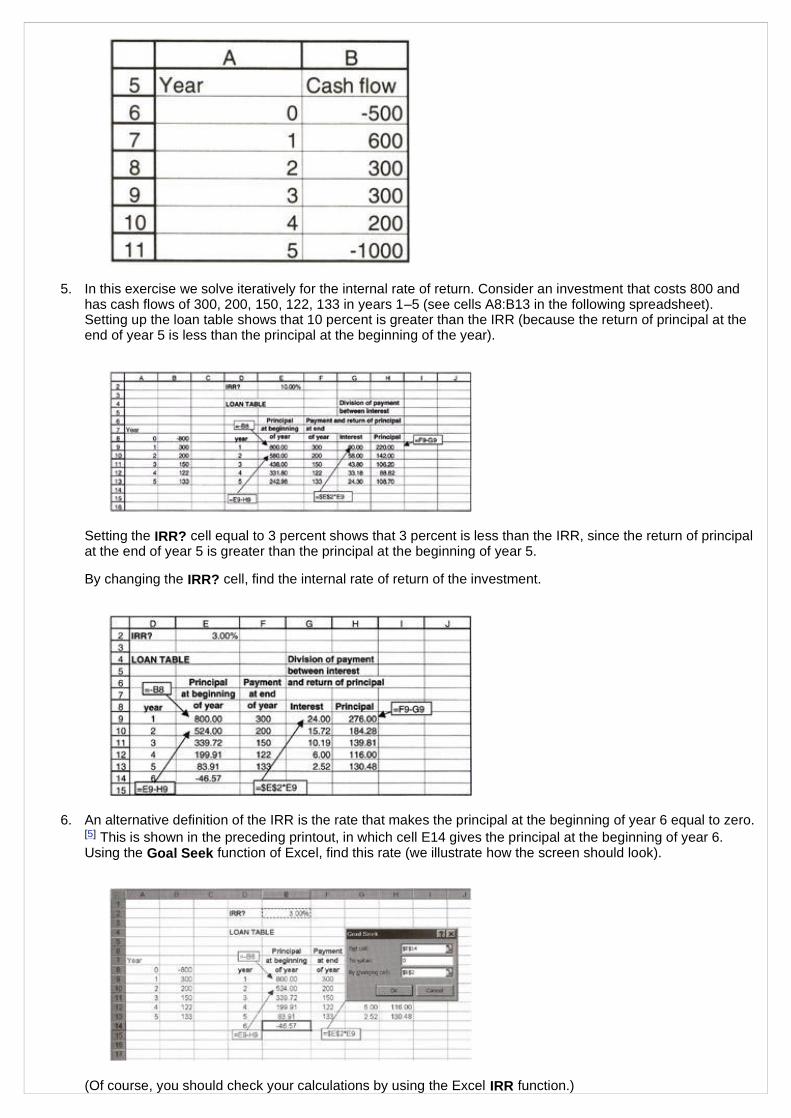
5. In this exercise we solve iteratively for the internal rate of return. Consider an investment that costs 800 andhas cash flows of 300, 200, 150, 122, 133 in years 1–5 (see cells A8:B13 in the following spreadsheet).Setting up the loan table shows that 10 percent is greater than the IRR (because the return of principal at theend of year 5 is less than the principal at the beginning of the year).

Setting the IRR? cell equal to 3 percent shows that 3 percent is less than the IRR, since the return of principalat the end of year 5 is greater than the principal at the beginning of year 5.

By changing the IRR? cell, find the internal rate of return of the investment.

6. An alternative definition of the IRR is the rate that makes the principal at the beginning of year 6 equal to zero.[5] This is shown in the preceding printout, in which cell E14 gives the principal at the beginning of year 6.Using the Goal Seek function of Excel, find this rate (we illustrate how the screen should look).

(Of course, you should check your calculations by using the Excel IRR function.)

7. Calculate the flat annual payment required to pay off a five-year loan of $100,000 bearing an interest rate of13 percent.

8. You have just taken a car loan of $15,000. The loan is for 48 months at an annual interest rate of 15 percent(which the bank translates to a monthly rate of 15 percent/12 = 1.25 percent). The 48 payments (to be madeat the end of each of the next 48 months) are all equal.

a. Calculate the monthly payment on the loan.

b. In a loan table, calculate, for each month, the principal remaining on the loan at the beginning of themonth and the split of that month's payment between interest and repayment of principal.

c. Show that the principal at the beginning of each month is the present value of the remaining loanpayments at the loan interest rate (use the PV function).

9. You are considering buying a car from a local auto dealer. The dealer offers you one of two payment options:

n You can pay $30,000 cash.

n The "deferred payment plan": You can pay the dealer $5,000 cash today and a payment of $1,050 at theend of each of the next 30 months.

As an alternative to the dealer financing, you have approached a local bank, which is willing to give you a carloan of $25,000 at the rate of 1.25 percent per month.

a. Assuming that 1.25 percent is the opportunity cost, calculate the present value of all the payments onthe dealer's deferred payment plan.

b. What is the effective interest rate being charged by the dealer? Do this calculation by preparing aspreadsheet like this (only part of the spreadsheet is shown—you have to do this calculation for all 30months):

Now calculate the IRR of the numbers in column F; this is the monthly effective interest rate on the deferredpayment plan.

10. You are considering a savings plan that calls for a deposit of $15,000 at the end of each of the next five years.If the plan offers an interest rate of 10 percent, how much will you accumulate at the end of year 5?

Do this calculation by completing the following spreadsheet. This spreadsheet does the calculation twice—once using the FV function and once using a simple table that shows the accumulation at the beginning ofeach year.

11. Redo the calculation of exercise 10, this time assuming that you make five deposits at the beginning of thisyear and the following four years. How much will you accumulate by the end of year 5?

12. A mutual fund has been advertising that, had you deposited $250 per month in the fund for the last 10 years,you would now have accumulated $85,000. Assuming that these deposits were made at the beginning ofeach month for a period of 240 months, calculate the effective annual return fund investors got.

Hint Set up the following spreadsheet, and then use Goal Seek

The effective annual return can then be calculated in one of two ways:1. (1 + Monthly return)12 − 1: This is the compound annual return, which is preferable, since it makes

allowance for the reinvestment of each month's earnings.

2. 12 * Monthly return: This method is often used by banks.

13. You have just turned 35, and you intend to start saving for your retirement. Once you retire in 30 years (whenyou turn 65), you would like to have an income of $100,000 per year for the next 20 years. Calculate howmuch you would have to save between now and age 65 in order to finance your retirement income. Make thefollowing assumptions:

n All savings draw compound interest of 10 percent per year.

n You make the first payment today and the last payment on the day you turn 64 (30 payments).

n You make the first withdrawal when you turn 65 and the last withdrawal when you turn 84 (20 payments).

14. You have $25,000 in the bank, in a savings account that draws 5 percent interest. Your business needs$25,000, and you are considering two options: (a) Use the money in your savings account or (b) borrow themoney from the bank at 6 percent, leaving the money in your savings account.

Your financial analyst suggests that solution (b) is better. His logic: The sum of the interest paid on the 6percent loan is lower than the interest earned at the same time on the $25,000 deposit. His calculations areillustrated in the following spreadsheet. Show that this logic is wrong. (If you think about it, it couldn't bepreferable to take a 6 percent loan when you are getting 5 percent interest from the bank. However, theexplanation for this may not be trivial.)

[5]In general, of course, the IRR is the rate of return that makes the principal in the year following the last paymentequal to zero.


Chapter 2: Calculating the Cost of Capital

2.1 IntroductionThe most widely used valuation method for firms is the discounted cash flow (DCF) method. In the next two chapterswe show how to use integrated accounting-based financial models for the firm to calculate the firm's free cash flows.Discounting these cash flows at an appropriately risk-adjusted discount rate will give us the value of the firm.

In this chapter we discuss how to calculate the firm's cost of capital, the discount rate applied to future cash flows.We consider two models for calculating the cost of equity, the discount rate applied to equity cash flows:

n The Gordon model calculates the cost of equity based on the anticipated dividends of the firm.

n The capital asset pricing model (CAPM) calculates the cost of equity based on the correlation between the firm'sequity returns and the returns of a large, diversified, market portfolio. As we will see, the CAPM can also beused to calculate the cost of the firm's debt.

The other component of the cost of capital is the cost of debt, the anticipated future cost of the firm's borrowing. Weillustrate three models to calculate the cost of debt.

We use all of these models to calculate the weighted average cost of capital (WACC), the appropriate discount ratefor valuation of firm cash flows. Throughout this chapter we apply our techniques to calculating the cost of capital forAbbott Laboratories.

A Terminological Note As noted in the previous chapter, "cost of capital" is a synonym for the "appropriate discountrate" to be applied to a series of cash flows. In finance, "appropriate" is most often a synonym for "risk-adjusted."Hence, another name for the cost of capital is the "risk-adjusted discount rate" (RADR).

Chapter 2 - Calculating the Cost of Capital




2.2 The Gordon Dividend ModelThe Gordon dividend model[1] derives the cost of equity from the following deceptively simple statement:

The value of a share is the present value of the future anticipated dividend stream from the share, where the futureanticipated dividends are discounted at the appropriate risk-adjusted cost of equity.

Consider, for example, the case of a stock whose dividends are anticipated to grow at 10 percent per year. If nextyear's anticipated dividend is $3 per share, then the value of the stock today, P0, is given by

The formula in cell B6 of the following spreadsheet discounts 67 years of dividends (not all for which are shown):

Notice that our "solution" is really only an approximation. We've simply taken the NPV for a very long series ofdividends, whereas the actual problem in the equation relates to an infinite series of dividends. To do this infinite-series calculation, we need to resort to some manipulation of the formula. We rewrite the formula using D1 to denotethe next period anticipated dividend and using g to denote the anticipated growth rate of dividends:

The last equality, P0 = , was derived by the Swiss mathematician Leonhard Euler (1707–83), and itsderivation (which we won't give here) is a staple of high-school algebra classes. Note the proviso at the end: In order




for the infinite sum on the first line of the formula to have a finite solution, the growth rates of the dividends must beless than the discount rate. We can use this formula in our spreadsheet:

So—if the dividend to be paid one year from now is anticipated to be $3, and if this dividend is expected to grow by10 percent per year, and if the correct discount rate is 15 percent, then the value of the share should be $60. We canfix the technical problem by redefining the formula, as in the following spreadsheet:

2.2.1 "Supernormal Growth" and the Gordon ModelNotice that if the condition |g| < rE is violated, the formula P0 = D1/ (rE − g) gives a negative answer. However, thisdoes not mean that the value of the share is negative; rather it means that the basic condition has been violated. Infinance examples, violations of |g| < rE usually occur for very fast-growing firms, in which—at least for short periodsof time—we anticipate very high growth rates, so that g>rE. In this case the original dividend discount formula showsthat P0 will have an infinite value. Since this result is clearly unreasonable (remember that we are valuing a security),it probably means either (1) that the long-term growth rate is less than the discount rate rE, or (2) that the discountrate rE is too low.

The following spreadsheet illustrates an initial, very high, growth rate that ultimately slows to a lower rate. Weconsider a firm whose current dividend is $8 per share. The firm's dividend is expected to grow at 35 percent for thenext five years, after which the growth rate will slow down to 8 percent per year. The cost of equity, the discount ratefor all of the dividends, is 18 percent:

To calculate the value of the firm's share, we first discount the dividends for years 1–5. Cell E4 shows that these fivefuture dividends are worth $40. Now look at years 6–∞. Denote the long-term growth rate by g2 (in our example thisis 8 percent). At time 0, the discounted dividend stream from years 6–∞ looks like:

This last expression is basically the Gordon model discounted over five years.

As shown in the spreadsheet, the value of the share is estimated at 230.33.

2.2.2 Back to the Gordon Model with Constant Growth RatesNow we return to the Gordon model with a single growth rate. Since in this model P0 = D1/(rE − g), we can rearrangethe formula to give us the cost of equity rE:

Often we assume that the D1 = D0(1 + g), where D0 is the last dividend the firm has paid; in this case the Gordonmodel is written

[1]This model is named after M. J. Gordon, who first published this formula in a paper entitled "Dividends, Earningsand Stock Prices," Review of Economics and Statistics 41 (May 1959), pp. 99–105.


2.3 Calculating the Cost of Equity for Abbott Laboratories Using the GordonModelIn the following spreadsheet you can see the dividend history of Abbott Laboratories from 1988 to 1998. Thecompound growth rate of Abbott's dividends over the period is 14.87 percent (and the five-year growth rate is 12.03percent). Abbott's stock price at the end of 1998 was $49. Applying the Gordon formula gives (cells J22 and J23)Abbott's cost of equity as 16.28 percent or 13.4 percent depending on which growth rate we use.

2.3.1 Choosing the Growth Rate in the Gordon ModelThe growth rate g in the Gordon formula is the anticipated rate of dividend growth, which is not necessarily thehistorical growth rate of dividend. Thus the "correct" growth rate is a judgment call—it depends on your expectationsof what the company can and will pay out in dividends in the future. [2] In the case of Abbott Labs, we might decidethat the five-year growth rate is more representative of future anticipated dividend growth than the 10-year rate. Inthis case, the cost of equity would be 13.40 percent instead of 16.28 percent. (Based on a more extensive analysisof Abbott, you might decide that the historical rate of Abbott's dividend growth has no relevance for its future dividendgrowth rate. This is one of the hard decisions that analysts have to make!)

[2]The pro forma financial statements discussed in the next chapter can sometimes help in this matter. By anticipatingfuture sales growth and capital needs for the company, we can perhaps predict the company's future dividend.





2.4 Capital Asset Pricing ModelThe capital asset pricing model (CAPM) is the other viable alternative to the Gordon model for calculating the cost ofcapital. The CAPM derives the firm's cost of capital from its covariance with the market return.[3] In the following tablewe show part of a 10-year price and return history for Abbott Labs and the S&P 500 index (the actual β calculationwas done with 10 years of data—see the spreadsheet on the book CD-ROM).

Abbott's beta, βAbbott, shows the sensitivity of its stock return to the market return. It is calculated by the followingformula:

In cell J5 of the spreadsheet fragment in section 2.5.1 we show that Abbott's β is 0.8055.

Another way of calculating the β is to graph the S&P 500 returns on the x-axis and to graph the Abbott stock returnson the y-axis and then use the Excel Trendline function to calculate the regression equation:




The regression equation in the graph shows the best linear function that explains the Abbott's returns (the y in theequation) in terms of the S&P 500 returns (the x on the right-hand side of the equation).[4] The regression equationshows that, during 1997, a 1 percent increase or decrease in the S&P 500 return led to a 0.8055 percent increase ordecrease in Abbott's return. The R2 = 0.3348 says that about 33 percent of the variation in Abbott's returns wasexplained by the variation in the S&P 500 returns.[5]

[3]The CAPM is discussed in detail in Chapters 7–11. At this point we outline the application of the model to findingthe cost of capital without entering into the theory.

[4]The use of Excel's Trendline function—used to calculate the regression equation—is further explained in Chapter29.

[5]An R [2] of 33 percent may seem low, but in the CAPM literature this is actually quite a respectable number. It saysthat roughly 33 percent of the variation in Abbott's returns is explicable by the variation in the S&P 500 return. Therest of the variability in the Abbott returns can be diversified away by including Abbott's shares in a diversifiedportfolio of shares.


2.5 Using the Security Market Line (SML) to Calculate Abbott's Cost of EquityIn the capital asset pricing model, the security market line (SML) is used to calculate the risk-adjusted cost of capital.In this section we consider two SML formulations. The difference between these two methods has to do with the waytaxes are incorporated into the cost of capital equation.

2.5.1 Method 1: The Classic SMLThe classic CAPM formula uses a security market line (SML) equation that ignores taxes.

Here rf is the risk-free rate of return in the economy and E(RM) is the expected rate of return on the market. Thechoice of values for the SML parameters is often problematic. A common approach is to choose

n rf equal to the risk-free interest rate in the economy (for example, the yield on Treasury bills).

n E(rM) − rf equal to the historic average of the "market risk premium," defined as the average return of a broad-based market portfolio minus the risk-free rate.

The following spreadsheet fragment illustrates this approach.

2.5.2 Method 2: The Benninga-Sarig Tax-Adjusted SMLThe classic CAPM approach makes no allowance for taxation. Benninga-Sarig (1997) show that the SML has to beadjusted for the marginal corporate tax rate in the economy. Denoting the corporate tax rate by TC, the Benninga-Sarig tax-adjusted SML is

This formula can be applied by an adaptation of the previous approach:

n rf is equal to the risk-free interest rate in the economy (in this case, the yield on Treasury bills).

n E(rM) − rf(1 − TC) = [E(rM) − rf] + TCrf , which is equal to the historic average of the market risk premium plus TCrf.

For Abbott Labs, the Benninga-Sarig approach gives a slightly lower cost of equity:




2.5.3 Calculating the Expected Return on the Market, E(rM): Using the GordonModelThe 8.40 percent figure for E (rM) − rf approximates the historic market risk premium in the United States for 1926–1994. On the one hand, historic averages are appropriate if we think that the future anticipated rates of return willcorrespond to the historic average. On the other hand, we may want to take current market data to calculate directlythe future anticipated market yield.

As Benninga and Sarig show, the Gordon model gives us an approach for doing so. [6] Recall that the model saysthat the cost of equity rE is given by

Rewriting this formula, assuming that the firm pays out a constant proportion a of its earnings as dividends, indicatingby EPS0 the current earnings per share, and interpreting g to be the earnings growth of the firm:

The term on the right-hand side of this equation P0/EPS0 is the price-earnings ratio of the firm. This formula ties thecost of equity to currently observable market parameters. Here is an implementation for calculating Abbott's cost ofequity:

[6]A fuller exposition of this model can be found in Chapter 8 of Corporate Finance: A Valuation Approach by SimonBenninga and Oded Sarig (McGraw-Hill, 1997).


2.6 Calculating the Cost of DebtThus far we have calculated the cost of equity for the Abbott Labs. We now want to calculate the cost of the firm'sdebt. In principle, this is the marginal cost to the firm (before corporate taxes) of borrowing an additional dollar. Inpractice the cost of debt often turns out to be more difficult to calculate than the cost of equity. There are at least fourways of calculating the firm's cost of debt. We will state them briefly and then go on to illustrate the application ofthree of the methods to Abbott Labs. The first two methods are easy to apply and, although they may not betheoretically perfect, they are often used in practice.

n As a practical matter, the cost of debt can often be approximated by taking the average cost of the firm's existingdebt. Although this method is the easiest to use, it confuses past costs with the future anticipated cost of debtthat we actually want to measure.

n We can use the yield of similar-risk corporate securities. If a company is rated A and has mostly medium-termdebt, then we can use the average yield on medium-term, A-rated debt as the firm's cost of debt. Note that thismethod is somewhat problematic because the yield on a bond is its promised return, whereas the cost of debt isthe expected return on a firm's debt. Since there is usually a risk of default, the promised return is generallyhigher than the expected return.

Both these methods are relatively easy to apply. In many cases problems or errors that are encountered in thesemethods are not critical.[7] As a matter of theory, however, both these methods fail to make proper riskadjustments for the cost of the firm's debt. The next two methods make risk adjustments but are harder to apply:

n The CAPM can be applied to the cost of capital by estimating the β of the firm's debt. We can then estimate thefirm's cost of debt by using the security market line (SML). This approach is, in principle, similar to the processapplied to the firm's equity, although—as we will show—the actual application requires many shortcuts andfuzzinesses.

n We can use a model that estimates the cost of debt from data about the firm's bond prices, the estimatedprobabilities of default, and the estimated payoffs to bondholders in case of default. This method requires a lot ofwork and is mathematically nontrivial; we postpone its discussion until Chapter 23. For cost of capitalcalculations it would be used in practice only if the firm we are analyzing has significant amounts of risky debt.

[7]Calculating the cost of capital requires a large number of assumptions and does not necessarily give a preciseanswer. Thus cost of capital estimation is not a science, it is an art. Users of cost of capital estimates should alwaysdo a sensitivity analysis around the numbers calculated. Given the data on the company you are analyzing, somesloppiness in the cost of capital calculations (with its accompanying savings in time) may be expedient.





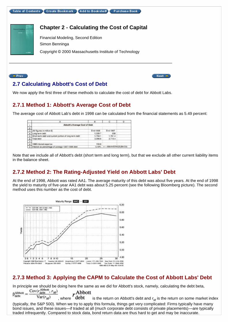
2.7 Calculating Abbott's Cost of DebtWe now apply the first three of these methods to calculate the cost of debt for Abbott Labs.

2.7.1 Method 1: Abbott's Average Cost of DebtThe average cost of Abbott Lab's debt in 1998 can be calculated from the financial statements as 5.49 percent:

Note that we include all of Abbott's debt (short term and long term), but that we exclude all other current liability itemsin the balance sheet.

2.7.2 Method 2: The Rating-Adjusted Yield on Abbott Labs' DebtAt the end of 1998, Abbott was rated AA1. The average maturity of this debt was about five years. At the end of 1998the yield to maturity of five-year AA1 debt was about 5.25 percent (see the following Bloomberg picture). The secondmethod uses this number as the cost of debt.

2.7.3 Method 3: Applying the CAPM to Calculate the Cost of Abbott Labs' DebtIn principle we should be doing here the same as we did for Abbott's stock, namely, calculating the debt beta,

, where is the return on Abbott's debt and rM is the return on some market index(typically, the S&P 500). When we try to apply this formula, things get very complicated: Firms typically have manybond issues, and these issues—if traded at all (much corporate debt consists of private placements)—are typicallytraded infrequently. Compared to stock data, bond return data are thus hard to get and may be inaccurate.




In practice the β of corporate debt relates to two factors:1. The maturity of the debt. The longer the term of a firm's debt, the more risky it is.

2. The default risk of the debt. The greater the default risk, the greater is the debt β.

For many corporate debt issues, the first factor is more important than the second. For a relatively highly ratedcompany like Abbott, this factor is dominant.

A good rule of thumb for estimating the firm's debt β is the following (these numbers—very crude estimates—arejustified somewhat in the appendix to this chapter):

Abbott Labs is a low-risk company. Its average debt maturity is on the low side of the medium-term debt. We canthus plug its debt β as βdebt = 0.15. As in the case of the CAPM calculations for equity, there are two models withwhich to calculate the cost of debt. The classic CAPM formulation is that the cost of debt is calculated using thefollowing security market line (SML):

The Benninga-Sarig tax-adjusted cost of debt SML for debt is

The following spreadsheet fragment illustrates both calculations:

Term Riskiness Bond Beta

Very short Low 0

Short (1–3 years) Low 0.1

Medium (3–10 years) Intermediate 0.35

Long (> 10 years) Low 0.6

Long (> 10 years) Intermediate 0.8


2.8 Weighted Average Cost of Capital (WACC)The preceding examples for the Gordon dividend model and the CAPM derive the cost of equity, the risk-adjusteddiscount rate that should be applied to the firm's equity payouts to shareholders. The discount rate that should beapplied to the firm's free cash flows—the cash flows of the firm as a whole—is called the weighted average cost ofcapital (WACC). The WACC is a weighted average of the cost of equity and the cost of debt.

where E is the market value of the firm's equity, D is the market value of the firm's debt, and TC is the corporate taxrate.

In the next spreadsheet we calculate Abbott's WACC for the case where the cost of debt is calculated by Method 1but where we use both the Gordon model and the CAPM for the cost of equity:





2.9 When the Models Don't WorkAll models have problems, and nothing is perfect.[8] In this section we discuss some of the potential problems withthe Gordon model and with the capital asset pricing model.

2.9.1 Problems with the Gordon ModelObviously the Gordon model doesn't work if a firm doesn't pay dividends and appears to have no intention—in theimmediate future—of paying dividends.[9] But even for dividend-paying firms, it may be difficult to apply the model.Particularly problematic, in many cases, is the extraction of the future dividend payout rate from past dividends.

Consider, for example, the dividend history of Ford Motor Company in the years 1989–98:

The problem here is easily identifiable: Ford, whose dividends were in steady decline until 1997, paid a cashdividend of $21.09 in 1998, in addition to its regular quarterly dividends (which summed to $1.72 in 1998). If we usepast history to predict the future, any inclusion of the extraordinary cash dividend will cause us to overestimate thefuture dividend growth. Excluding the $21.09 dividend, however, also does not reflect the actual situation.

It appears that the 10-year history of Ford's dividends is not, perhaps, the best guide to its future dividend payout.There are several solutions for those wishing to use the Gordon model:

n If we exclude the extraordinary dividend of $21.09 in 1998, then the dividend growth over the four years endingin 1998 is a respectable 6.64 percent. If Ford's anticipated future dividend growth is estimated to be this rate,then—given its end-1998 stock price of $58.69—the Gordon-model cost of equity is 9.77 percent.




n A second alternative to finding Ford's cost of capital is to predict its future dividends by doing a full-blownfinancial model for the company. Such models—illustrated in the succeeding two chapters—are often used byanalysts. Though they are complicated and time-consuming to build, they take into account all of the firm'sproductive and financial activities. Potentially they are, therefore, a more accurate predictor of the dividend.

2.9.2 Problems with the CAPMIn the following spreadsheet fragment you will find the return of the S&P 500 and Big City Bagels (notice that thespreadsheet fragment skips from row 8 to row 35—some of the rows of the data have been hidden). Immediatelyafter the spreadsheet is a graph that shows the calculation of Big City's β, which is computed to be −0.6408.

Big City Bagel's stock is clearly risky—the annualized standard deviation of its returns is 152 percent as compared toabout 17 percent for the S&P 500 over the same period. However, the β of Big City Bagels is −0.6408, indicating thatBig City has—in a portfolio context—negative risk. Were this conclusion true, it would mean that adding Big City to aportfolio would lower the portfolio variance enough to justify a below-risk-free return for Big City. While this statementmight be true for some stocks, it is hard to believe that—in the long run—the β of Big City is indeed negative.[10]

The R2 of the regression between Big City's returns and the S&P 500 is extraordinarily low, 0.0052, meaning that theS&P 500 simply doesn't explain any of the variation in Big City returns. For statistics mavens: The situation isactually worse—the standard error of the slope estimate is 1.57, which is 2.5 times larger than the slope itself

(meaning that the slope estimate is not statistically significantly different from zero).

What are we to make of this situation? How should we calculate the cost of capital for Big City? There are severalalternatives.

n We could assume that the Big City β is −0.6408. Depending on which version of the CAPM you use, this wouldgive Big City's cost of equity as follows:

n We could assume that the β of Big City is in fact zero. Given the standard deviation of the β estimate for BigCity, the β is not statistically different from zero, so that this assumption makes sense. We can conclude that allof Big City's risk is diversifiable and that the correct cost of equity for Big City is the riskless rate of interest.

n We could assume that the covariance (or lack thereof) between Big City and the S&P 500 is not indicative oftheir future correlation. This assumption would eventually lead us to conclude that Big City's risk is comparableto that of similar companies. A small study of the βs of snack food companies shows their βs to be well over 1:New World Coffee has a β of 1.15, Pepsico has a β of 1.42, and Starbucks has a β of 1.84. Thus we mightconclude that the β of Big City (in the sense of its future correlation with the market) would be somewherebetween 1.15 and 1.84.

[8]"Happiness is the maximum agreement of reality and desire."—Stalin.

[9]Firms cannot intend never to pay dividends, because such an intention would rationally mean that the value of theshares is zero.

[10]A more plausible explanation is that—for the period covered—Big City's return has nothing whatsoever to do withthe market return.


2.10 ConclusionIn this chapter we have illustrated in detail the application of two models for calculating the cost of equity: the Gordondividend model and the CAPM. We have also considered three of the four practicable models for calculating the costof debt. Because the application of these models includes many judgment calls, our advice is to

n Always use several models to calculate the cost of capital.

n If you have time, try to calculate the cost of capital not only for the firm you are analyzing, but also for other firmsin the same industry.

n From your analysis try to pick out a consensus estimate of the cost of capital. Don't hesitate to exclude numbers(such as Big City's negative cost of equity) that strike you as unreasonable.

In sum, the calculation of the cost of capital is not just a mechanistic exercise!

Exercises1. ABC Corp. has a stock price P0 = 50. The firm has just paid a dividend of $3 per share, and knowledgable

shareholders think that this dividend will grow by a rate of 5% per year. Use the Gordon dividend model tocalculate the cost of equity of ABC.

2. Unheardof, Inc. has just paid a dividend of $5 per share. This dividend is anticipated to increase at a rate of15% per year. If the cost of equity for Unheardof is 25%, what should be the market value of a share of thecompany?

3. Dismal.com is a producer of depressing Internet products. The company is not currently paying dividends, butits chief financial officer thinks that starting in 3 years it can pay a dividend of $15 per share, and that thisdividend will grow by 20% per year. Assuming that the cost of equity of Dismal.com is 35%, value a sharebased on the discounted dividends.

4. Consider the following dividend and price data for Chrysler Corporation:




Use the Gordon model to calculate Chrysler's cost of equity in 1996.

5. On the spreadsheet associated with this chapter you will find the following monthly data for IBM's stock priceand the S&P 500 index during 1998:

a. Use these data to calculate IBM's β.

b. Suppose that at the end of 1997, the risk-free rate was 5.50 percent. Assuming that the market riskpremium, E (rm)−rf = 8 percent and that the corporate tax rate TC = 40 percent, calculate IBM's cost ofequity using both the classic CAPM security market line and Benninga-Sarig's tax-adjusted securitymarket line.

c. At the end of 1997, IBM had 969,015,351 shares outstanding and had $39.9 billion of debt. Assumingthat IBM's cost of debt is 6.10 percent, use your calculations for the cost of equity in part b to arrive attwo estimates of IBM's weighted average cost of capital.

6. A firm has a current stock price of $50 and has just paid a dividend of $5 per share.a. Assuming that investors in the firm anticipate a dividend growth rate of 10 percent, what is the firm's

cost of equity?

b. Draw a graph showing the relation between the cost of equity and the anticipated dividend growth rate.

7. Exercise on supernormal growth: ABC Corporation has just paid a dividend of $3 per share. You—anexperienced analyst—feel quite sure that the growth rate of the company's dividends over the next 10 yearswill be 15 percent per year. After 10 years you think that the company's dividend growth rate will slow to theindustry average, which is about 5 percent per year. If the cost of equity for ABC is 12 percent, what is thevalue today of one share of the company?

8. Consider a company that has βequity = 1.5 and βdebt = 0.4. Suppose that the risk-free rate of interest is 6percent, the expected return on the market E(rm) is 15 percent and the corporate tax rate is 40 percent. If thecompany has 40 percent equity and 60 percent debt in its capital structure, calculate its weighted averagecost of capital using both the classic CAPM and the Benninga-Sarig tax-adjusted CAPM.

9. You are considering buying the bonds of a very risky company. A bond with a $100 face value, a one-yearmaturity, and a coupon rate of 22% is selling for $95. You consider the probability that the company willactually survive to pay off the bond 80%. With 20% probability, you think that the company will default, inwhich case you think that you will be able to recover $40. What is the expected return on the bond?

10. It is January 1, 1997. Normal America, Inc. (NA) has paid a year-end dividend in each of the last 10 years, asshown by the following table.

Calculate NA's β with respect to the SP500.

Appendix 1: A Rule of Thumb for Calculating Debt BetasVanguard is a large manager of mutual funds. Among its funds is the Vanguard Index 500 fund, which tracks theS&P 500 portfolio. The company also has numerous bond funds. The following table shows the β of these bondfunds derived by calculating the

for each fund. When we do this calculation for a number of Vanguard funds, we get the following results.

Regressing the β on the bond fund average maturity gives:

The rules of thumb for debt betas in the chapter are based on this regression.

The regression results can be seen in the following graph:

Appendix 2: Why Is β Such a Good Measure of Risk? Portfolio β versusIndividual Stock βAlthough β may not be a very good measure of the riskiness of an individual stock, the average β is a very goodmeasure of the riskiness of a diversified portfolio. This point is illustrated in this appendix. However, before we fireinto the illustration, we want to stress the meaning of the first sentence:

If portfolio β is a good measure of portfolio risk, then—for holders of diversified portfolios (and these include mostinvestors)—the individual-share β is a good measure of the risk of a share, when this share is ultimately held in adiversified portfolio.

To illustrate, consider the following graph, which gives the βs of 23 shares.[11] As you can see, the R2 for theindividual regressions are not high (the highest R2 is 35 percent and the lowest is close to zero). The average R2 forthe 23 stocks is 16.05 percent, and the average β is 0.944.

When we combine the 23 shares into an equally weighted portfolio, the portfolio β is 0.944, which is equal to theaverage beta of the component securities.[12] However, the portfolio's R2 = 61.44 percent, which is much larger thanaverage R2 of the component securities. For a large, well-diversified portfolio, the portfolio R2 approaches 1.

The meaning of this number is that—when we invest in large diversified portfolios—almost all of the risk is due to the

individual assets' βs.

Appendix 3: Getting Data from the InternetAll of the data used in this chapter were retrieved from the Internet. This appendix provides a brief description of howthey were obtained. Keep in mind that, since the Internet is a very lively place, some of the technical details andaddresses may have changed by the time you read this book.

1. By going to the Yahoo business news page (http://dailynews.yahoo.com/headlines/business/) you canindicate in the Get Quotes window the ticker symbol of the company you want to look up. In the followingpicture, I have asked for information on abt, the symbol for Abbott Laboratories.

2. Clicking on the Get Quotes box gives you the company's latest stock quote.

3. Clicking on Profile (in the box labeled More Info) gives a page of basic financial information about thecompany, including its β.

Note that the β for Abbott is not the same as the one calculated in the chapter. There are two reasons for thisdifference: First, the chapter uses return data that include dividends, whereas the calculation on Yahooexcludes dividends. Second, the time horizon is different—the Yahoo calculation uses five years of data,whereas the calculations in the chapter are based on 10 years.

Note also that the page can direct you to much more information about Abbott. The company's Web site hasall its financial statements in downloadable form.

4. To get downloadable price information on Abbott Labs in Yahoo, click on Chart in the Basic Info box. You willthen see a page like the following:

5. Clicking on Table and choosing the appropriate time interval (here we chose monthly) gives you thefollowing:

Clicking on Download Spreadsheet Format gives the data (already adjusted for dividends and splits) in a csv filethat can be opened with Excel. Note that you can change the Start Date and the End Date for the data.

Final Note Ticker symbols for two indexes commonly used: ^SPX (S&P 500), ^DJI (the Dow-Jones 30 Industrials).

[11]β is calculated against return data for the S&P 500 for monthly return data from July 1994 through June 1999.

[12]This equality will always hold: Suppose we take n securities whose βs are β1, β2,…βn. Now suppose we take a

portfolio in which the weight of each security is x1, x2, …xn, where . Then the portfolio β will be equal to the

weighted average of the individual security βs: βportfolio = .

Chapter 3: Financial Statement Modeling

3.1 OverviewThe usefulness of financial-statement projections for corporate financial management is undisputed. Suchprojections, termed pro forma financial statements, are the bread and butter of much corporate financial analysis. Inthis and the next chapter we will focus of the use of pro formas for valuing the firm and its component securities, butpro formas also form the basis for many credit analyses; by examining pro forma financial statements we can predicthow much financing a firm will need in future years. We can play the usual "what if" games of simulation models, andwe can use pro formas to ask what strains on the firm may be caused by changes in financial and sales parameters.

In this chapter we present a variety of financial models. All the models are sales driven, in that they assume thatmany of the balance-sheet and income-statement items are directly or indirectly related to sales. The mathematicalstructure of solving the models involves finding the solution to a set of simultaneous linear equations predicting boththe balance sheets and the income statements for the coming years. However, the user of a spreadsheet need neverworry about the solution of the model; the fact that spreadsheets can solve—by iteration—the financial relations ofthe model means that we only have to worry about correctly stating the relevant accounting relations in our Excelmodel.[1]

[1]The mathematics of balance sheet spreadsheets involve an iterative method for solving simultaneous equationsknown as the Gauss-Seidel method. Although you do not need to know this method to understand the contents ofthis chapter, it may be interesting to know that Gauss-Seidel can be implemented directly in Excel. For details, seeChapter 28.

Chapter 3 - Financial Statement Modeling




3.2 How Financial Models Work: Theory and an Initial ExampleAlmost all financial-statement models are sales driven; this term means that as many as possible of the mostimportant financial statement variables are assumed to be functions of the sales level of the firm. For example,accounts receivable may be taken to be a direct percentage of the sales of the firm. A slightly more complicatedexample might postulate that the fixed assets (or some other account) are a step function of the level of sales:

etc.

In order to solve a financial-planning model, we must distinguish between those financial-statement items that arefunctional relationships of sales and perhaps of other financial-statement items and those items that involve policydecisions. The asset side of the balance sheet is usually assumed to be dependent only on functional relationships.The current liabilities may also be taken to involve functional relationships only, leaving the mix between long-termdebt and equity as a policy decision.

A simple example is the following. We wish to predict the financial statements for a firm whose current balance sheetand income statement are as follows:

The current (year 0) level of sales is 1,000. The firm expects its sales to grow at a rate of 10 percent per year. In




addition, the firm anticipates the following financial-statement relations.

3.2.1 The "Plug"Perhaps the most important financial policy variable in the financial statement modeling is the "plug": deciding whichbalance-sheet item will "close" the model. As an example, consider the balance sheet of our first pro forma model:

In this balance sheet we assume that that cash and marketable securities will be the plug. This assumption has twomeanings:

1. The mechanical meaning of the plug: Formally, we define

By using this definition, we guarantee that assets and liabilities will always be equal.

2. The financial meaning of the plug: By defining the plug to be cash and marketable securities, we are alsomaking a statement about how the firm finances itself. In our next model, for example, the firm sells noadditional stock, does not pay back any of its existing debt, and does not raise any more debt. This definitionmeans that all incremental financing (if needed) for the firm will come from the cash and marketable securitiesaccount; it also means that if the firm has additional cash, it will go into this account.[2]

3.2.2 Projecting Next Year's Balance Sheet and Income StatementWe have already given the financial statement for year zero. We now project the financial statement for year one:

Current assets: Assumed to be 15 percent of end-of-year sales

Current liabilities: Assumed to be 8 percent of end-of-year sales

Net fixed assets: 77 percent of end-of year sales

Depreciation: 10 percent of the average value of assets on the books during the year

Fixed assets at cost: Sum of net fixed assets plus accumulated depreciation

Debt: The firm neither repays any existing debt nor borrows any more money over thefive-year horizon of the pro formas.

Cash and marketablesecurities:

This is the balance sheet plug (see explanation that follows). Average balances ofcash and marketable securities are assumed to earn 8 percent interest.

Assets Liabilities and Equity

Cash and marketable securities Current liabilities

Current assets Debt

Fixed assetsFixed assets at cost - Accumulated depreciation

Net fixed assets

EquityStock (paid in capital)

Accumulated retained earnings

Total assets Total liabilities and equity

The formulas are mostly obvious. (The dollar signs—indicating that when the formulas are copied, the cell referencesto the model parameters should not change—are very important! If you fail to put them in, the model will not copycorrectly when you project years 2 and beyond.) Model parameters are in bold-face in the following list:

Income Statement Equations

n Sales = Initial sales * (1 + Sales growth)year

n Costs of goods sold = Sales * Costs of goods sold/Sales

The assumption is that the only expenses related to sales are costs of goods sold. Most companies also bookan expense item called selling, general, and administrative expenses (SG&A). The changes you would have tomake to accommodate this item are obvious (see an exercise at the end of this chapter).

n Interest payments on debt = Interest rate on debt * Average debt over the year

This formula allows us to accommodate changes in the model for repayment of debt, as well as rollover of debtat different interest rates. Note that in the current version of the model, debt stays constant; but in other versionsof the model to be discussed later debt will vary over time.

n Interest earned on cash and marketable securities = Interest rate on cash * Average cash and marketablesecurities over the year

n Depreciation = Depreciation rate * Average fixed assets at cost over the year

This calculation assumes that all new fixed assets are purchased during the year. We also assume that there isno disposal of fixed assets.

n Profit before taxes = Sales − Costs of goods sold − Interest payments on debt + Interest earned on cash andmarketable securities − Depreciation

n Taxes = Tax rate * Profit before taxes

n Profit after taxes = Profit before taxes − Taxes

n Dividends = Dividend payout ratio * Profit after taxes

The firm is assumed to pay out a fixed percentage of its profits as dividends. An alternative would be to assumethat the firm has a target for its dividends per share.

n Retained earnings = Profit after taxes − Dividends

Balance Sheet Equations

n Cash and marketable securities = Total liabilities − Current assets − Net fixed assets

As explained earlier, this formula means that cash and marketable securities are the balance sheet plug.

n Current assets = Current Assets/Sales * Sales

n Net fixed assets = Net fixed assets/Sales * Sales

n Accumulated depreciation = Previous year's accumulated depreciation + Depreciation rate * Average fixedassets at cost over the year.

n Fixed assets at cost = Net fixed assets + Accumulated depreciation

Note that this model does not distinguish between plant property and equipment (PP&E) and other fixed assetssuch as land.

n Current liabilities = Current liabilities/Sales * Sales

n Debt is assumed to be unchanged. An alternative model, which we will explore later, assumes that debt is thebalance-sheet plug.

n Stock doesn't change (the company is assumed to issue no new stock).

n Accumulated retained earnings = Previous year's accumulated retained earnings + Current year's additions toretained earnings

Financial statement models in Excel always involve cells that are mutually dependent. As a result, the solution ofthe model depends on the ability of Excel to solve circular references. To make sure your spreadsheetrecalculates, you have to go to the Tools|Options|Calculation box and click Iteration. If you open aspreadsheet that involves iteration, and if this box is not clicked, you will see the following Excel error message:

Depending on where you are in Excel when you open the file with the circular references, you may get a slightlydifferent version of this message. Whatever message you see, get out of it and go toTools|Options|Calculation|Iteration.In this dialog box click the box labeled Iteration:

3.2.3 Extending the Model to Years 2 and Beyond

Now that you have the model set up, you can extend it by copying the columns.

Note that the most common mistake to make in the transition between the two-columned financial model and thisone is the failure to mark the model parameters with dollar signs. If you commit this error, you will get zeros in placeswhere there should be numbers.

[2]The cash and marketable securities account can be viewed as a kind of "negative debt." We will return to this pointlater when we use the pro forma model to value the firm.


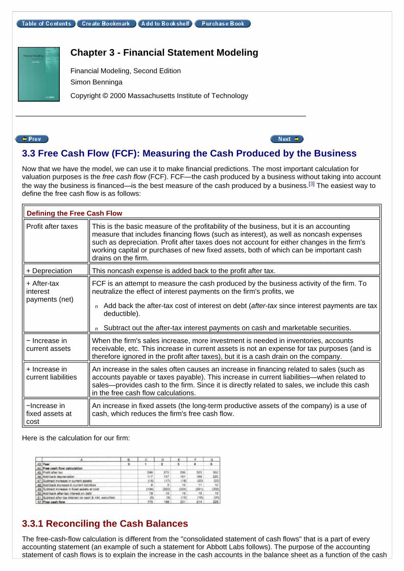
3.3 Free Cash Flow (FCF): Measuring the Cash Produced by the BusinessNow that we have the model, we can use it to make financial predictions. The most important calculation forvaluation purposes is the free cash flow (FCF). FCF—the cash produced by a business without taking into accountthe way the business is financed—is the best measure of the cash produced by a business.[3] The easiest way todefine the free cash flow is as follows:

Here is the calculation for our firm:

3.3.1 Reconciling the Cash BalancesThe free-cash-flow calculation is different from the "consolidated statement of cash flows" that is a part of everyaccounting statement (an example of such a statement for Abbott Labs follows). The purpose of the accountingstatement of cash flows is to explain the increase in the cash accounts in the balance sheet as a function of the cash




Defining the Free Cash Flow

Profit after taxes This is the basic measure of the profitability of the business, but it is an accountingmeasure that includes financing flows (such as interest), as well as noncash expensessuch as depreciation. Profit after taxes does not account for either changes in the firm'sworking capital or purchases of new fixed assets, both of which can be important cashdrains on the firm.

+ Depreciation This noncash expense is added back to the profit after tax.

+ After-taxinterestpayments (net)

FCF is an attempt to measure the cash produced by the business activity of the firm. Toneutralize the effect of interest payments on the firm's profits, we

n Add back the after-tax cost of interest on debt (after-tax since interest payments are taxdeductible).

n Subtract out the after-tax interest payments on cash and marketable securities.

− Increase incurrent assets

When the firm's sales increase, more investment is needed in inventories, accountsreceivable, etc. This increase in current assets is not an expense for tax purposes (and istherefore ignored in the profit after taxes), but it is a cash drain on the company.

+ Increase incurrent liabilities

An increase in the sales often causes an increase in financing related to sales (such asaccounts payable or taxes payable). This increase in current liabilities—when related tosales—provides cash to the firm. Since it is directly related to sales, we include this cashin the free cash flow calculations.

−Increase infixed assets atcost

An increase in fixed assets (the long-term productive assets of the company) is a use ofcash, which reduces the firm's free cash flow.

flows from the firm's operating, investing, and financing activities.

In the next example, we treat the cash and marketable securities account as if it were solely a cash account; we thenderive the increase in this account through a consolidated statement of cash flows:

Consolidated Statement of Cash Flows—Abbott Labs

Year ended December31

(dollars in thousands) 1998 1997 1996

Cash Flow from (Used in) Operating Activities:Net earnings $2,333,231 $2,094,462 $1,882,033

Adjustments to reconcile net earnings to net cash from operatingactivities—Depreciation and amortization

784,243 727,754 686,085

Exchange (gains) losses, net (14,176) 31,005 (3,419)

Investing and financing (gains) losses, net 90,798 113,999 57,224

Trade receivables (143,470) (222,427) (163,621)

Inventories (111,649) (98,964) (125,726)

Prepaid expenses and other assets (239,533) (491,769) (303,766)

Trade accounts payable and other liabilities 178,979 485,407 342,407

Income taxes payable (145,522) (10,700) 10,845

Net Cash from Operating Activities 2,732,901 2,628,767 2,382,062

Cash Flow from (Used in) Investing Activities:Acquisition of International Murex in 1998, Sanofi's parenteralproducts businesses in 1997, and MediSense in 1996, net ofcash acquired

(249,177) (200,475) (830,559)

Acquisitions of property, equipment and other businesses (990,619) (1,007,296) (949,028)

Purchases of investment securities (278,002) (25,115) (312,535)

Proceeds from sales of investment securities 78,898 43,424 117,783

Other 18,034 (8,209) 19,098

Net Cash Used in Investing Activities (1,420,866) (1,197,671) (1,955,241)

Cash Flow from (Used in) Financing Activities:Proceeds from (repayments of) commercial paper, net 42,000 402,000 317,000

Proceeds from issuance of long-term debt 400,000 — 500,000

Other borrowing transactions, net (59,499) 16,085 18,037

Purchases of common shares (875,407) (1,054,512) (808,816)

Proceeds from stock options exercised 150,881 137,482 109,638

Dividends paid (891,661) (809,554) (728,147)

Net Cash Used in Financing Activities (1,233,686) (1,308,499) (592,288)

Effect of exchange rate changes on cash and cash equivalents (143) (2,782) (5,521)

Net Increase (Decrease) in Cash and Cash Equivalents 78,206 119,815 (170,988)

Cash and Cash Equivalents, Beginning of Year 230,024 110,209 281,197

Cash and Cash Equivalents, End of Year $308,230 $230,024 $110,209

Supplemental Cash Flow Information:Income taxes paid $1,060,479 $922,242 $801,107

Interest paid 153,875 132,645 89,509

Line 77 checks that the changes in the cash accounts derived through the consolidated statement of cash flowsmatch those derived in the financial model (which uses cash as a plug).

[3]Extensive discussions of free cash flow and its uses in a valuation context can be found in books by Benninga andSarig (1997) and Copeland, Koller, and Murrin (1996).


3.4 Using the FCF to Value the Firm and Its EquityThe enterprise value of the firm is defined to be the value of the firm's debt, convertible securities, and equity. Infinancial theory, the enterprise value is the present value of the firm's future anticipated cash flows.

We can use the FCF projections and a cost of capital to determine the enterprise value of the firm. Suppose we havedetermined that the firm's weighted average cost of capital (WACC) is 20 percent (recall that the calculation of theWACC was discussed in Chapter 2). Then the enterprise value of the firm is the discounted value of the firm'sprojected FCFs plus its terminal value:

In this formula, the year-5 terminal value is a proxy for the present value of all FCFs from year 6 onward.[4]

Here's an example that uses our projections:

[4]We don't actually project these cash flows. Instead, as you will see in a moment, we determine the terminal valuebased on year-5 FCF.





3.5 Some Notes on the Valuation Procedure

3.5.1 Terminal ValueIn determining the terminal value we used a version of the Gordon model described in Chapter 2. We have assumedthat—after the year-5 projection horizon—the cash flows will grow at a rate equal to the sales growth of 10 percent.This assumption gives the terminal value as

The last equality is derived in a manner similar to the dividend valuation of shares (the Gordon model) discussed inChapter 2.

There are other ways of calculating the terminal value. All of the following are common variations that can beimplemented in the framework of our model (see end-of-chapter exercises):

n Terminal value = Year-5 book value of debt + Equity.

This calculation assumes that the book value correctly predicts the market value.

n Terminal value = (Enterprise market/book multiple) * (Year-5 book value of debt + Equity)

n Terminal value = P/E ratio * Year-5 profits + Year-5 book value of debt

n Terminal value = EBITDA ratio * Year-5 anticipated EBITDA (EBITDA = Earnings before interest, taxes,depreciation, and amortization.)

3.5.1.1 The Treatment of Cash and Marketable Securities in the ValuationNote that we have added the initial cash balances back to the present value of the projected FCFs to get theenterprise value. This procedure assumes the following:

n Year-0 balances of cash and marketable securities are not needed to produce the FCFs in subsequent years.

n Year-0 balances of cash and marketable securities are "surpluses" that could be drawn down or paid out toshareholders without affecting the future economic performance of the firm.

A wholly equivalent assumption sometimes made by investment bankers and equity analysts is to assume that initialcash balances are negative debt. If you made this assumption, you would value the equity in the following way:

3.5.2 Half-Year Discounting




While the NPV formula assumes that all cash flows occur at the end of the year, it is more logical to assume thatthey occur smoothly throughout the year. For discounting purposes, we should therefore discount cash flows as if, onaverage, they occur in the middle of the year. Thus the enterprise value is more logically calculated as follows:

Incorporating this half-year discounting into our value calculations gives


3.6 Sensitivity AnalysisAs in any Excel model, we can perform extensive sensitivity analysis on our valuation. Taking the last case as ourbase case, we can ask, for example, what is the effect of the sales growth rate on the equity value of the firm?

Cells B91:C100 contain a data table (see Chapter 26 if you are unsure of how to construct these tables). As youmight expect, the higher the sales growth, the higher the equity value of the firm.

Another variation is to calculate the effect on equity valuation of both the sales growth and the WACC. Here,however, you have to be careful: Examining the terminal value equation

will show you that this calculation only makes sense if the WACC is greater than the growth rate.[5] To overcome thisproblem we define the data table cell B107 (this is the calculation on which the data table does its sensitivityanalysis) in the following way:

[5]If the growth rate is greater than the WACC, then the terminal value is equal to .This problem was also discussed in Chapter 2 in the context of the Gordon dividend model.





3.7 Debt as a PlugIn the models that we have shown so far, cash and marketable securities were the plug and debt was a constant.However, for some values of the model parameters, you can get negative cash and marketable securities. Considerthe following example, which is still the same model, but—as indicated on the spreadsheet itself—with some differentparameter values.

Given these changes, the cash and marketable securities account (line 28) turns negative by year 2, a result which isobviously illogical. However, the economic meaning of these negative numbers is clear: Given the increased salesgrowth, increased current-asset and fixed-asset requirements, and increased dividend payouts, the firm needs morefinancing.[6]

What we want is a model which recognizes that

n Cash cannot be less than zero.

n When the firm needs additional financing, it borrows money.

Here is the model:




The equations for cash (line 28) and debt (line 37) are indicated for the year-5 entries. What they do in accountingterms is the following:

Cash and marketable securities remains the plug in the model.

The debt on the balance sheet conforms to the following test

n Current assets + Net fixed assets > Current liabilities + Last year's debt + Stock + Accumulated retainedearnings

If this relation holds, then there is no need to increase debt, and, in fact, the firm has to have positive cash andmarketable securities as a balancing item. The fact that we have made cash the plug will take care of thisconcern.

n Current assets + Net fixed assets < Current liabilities + Last year's debt + Stock + Accumulated retainedearnings

In this case, even if cash and marketable securities are equal to 0, we need to increase debt balances in orderto finance the firm's productive activities.

n In Excel programming terms, this formula becomes (for year 5, but each previous year has the same type ofequation) Max(G29+G33−G36−G38−G39,F37).

As shown in the exercises to this chapter, the model can easily accommodate a situation in which there are minimumcash balances.

[6]If you examine the model as it now stands, you will see that it implicitly assumes that this extra financing comes atthe cost of the cash and marketable securities. If we consider this account a kind of checking account with interest,then the model implicitly assumes that the firm can finance overdrafts from this account at the same rate of interestas it is being paid on the account.


3.8 Incorporating a Target Debt/Equity Ratio into a Pro FormaAnother change we might want to make in our model relates to the plug. Suppose that the firm has a target ratio ofdebt to equity: In each of the years 1–5 it wants debt and equity on the balance sheet to conform to a certain ratio.This situation is illustrated in the following example:

Line 42 of the spreadsheet shows the target debt/equity ratio in each of years 1–5. The firm wants to lower its currentdebt/equity ratio of 53 percent to 30 percent over the next two years. The relevant changes to the equations of ourinitial model are the following:

n Debt = Target debt/equity ratio * (Stock + Retained earnings)

n Stock = Total assets − Current liabilities − Debt − Accumulated retained earnings

Note that the firm will issue new debt in years 4 and 5; in year 1 the stock account grows (indicating that new equityis issued), whereas in subsequent years stock decreases (indicating a repurchase of equity).





3.9 Project Finance: Debt Repayment SchedulesHere is another use for pro forma modeling: In a typical case of so-called "project finance," the firm borrows money inorder to finance a project. The borrowing often comes with strings attached:

n The firm is not allowed to pay any dividends until the debt is paid off.

n The firm is not allowed to issue any new equity.

n The firm must pay back the debt over a specified period.

The following simplified example uses a variation of the version of our basic model with cash balances. A new firm orproject is set up; in year 0,

n The firm has assets of 2,200, which are financed with 100 of current liabilities, 1,100 of equity, and 1,000 ofdebt.

n The debt must be paid off in equal installments of principal over the next five years. Until the debt is paid off, thefirm is not allowed to pay dividends (if there is extra cash, it will go into a cash and marketable securitiesaccount).

The debt repayment terms are incorporated into the model by simply specifying the debt balances at the end of eachyear. Since the firm is assumed to issue no new equity (in accordance with the covenants on the lending), it followsthat the model's plug cannot be on the liabilities side of the balance sheet. In our model the plug is the cash andmarketable securities account.

The model incorporates one other assumption often made about fixed assets: It assumes that the net fixed assetsstay constant over the life of the project. As you can see from looking at lines 30–32, this assumption means that thefixed assets at cost grow each year by the increase in asset depreciation. It also means that in there is no net cash




flow from depreciation:

In this example the firm has no problem in making its debt principal repayments. As credit analysts, we might beinterested in how the firm's ability to meet its payments is affected by the various parameter values. In the followingexample we have increased the ratio of cost of goods sold to sales. With the new parameter values, the firm can nolonger meet its debt repayments in years 1–3. This fact can be seen in the pro forma: In years 1–3 the balances ofcash and marketable securities are negative, indicating that—in order to make the repayment of the loan principal—the firm had to borrow money.[7]

3.9.1 Calculating the Return on EquityEquity owners in the project have to pay 1,100 in year 0. During years 1–4 they get no payoffs, but in year 5 theyown the company. Suppose that the book value of the assets accurately reflects the market value. Then at the end ofyear 5 in the previous example the equity in the firm is worth Stock + Accumulated retained earnings = 2,255. Theexpected return on the equity investment (ROE) is calculated as follows:

It is interesting to note that this equity return increases as the equity investment decreases.[8] Consider the casewhere the firm initially borrows 1,500 and the equity owners invest 600:

As the following data table and graph show, the less the initial equity investment, the greater the equity return:

[7]From the point of view of corporate finance, positive balances of cash are like negative balances of debt. Thus,when the cash is negative, it is equivalent to the firm having borrowed money.

[8]Interesting but not surprising: As the equity investment goes down, the project becomes more leveraged andhence more risky for the equity investors. The increased return should compensate the equity holders for this extrarisk. The really interesting question (not answered here) is whether the increased return is in fact a compensation forthe riskiness.


3.10 ConclusionPro forma modeling is one of the basic skills of corporate financial analysis. Remember that financial modeling is adevious combination of finance, the implementation of accounting rules, and spreadsheet skills. In order to be useful,financial models must match the situation at hand, but they must also be simple enough so that the user can easilyunderstand why the results happen (be they valuations, creditworthiness, or simply commonsense predictions of howa firm or project might look several years down the road).

Exercises1. Here's a basic exercise that will help you understand what's going on in the modeling of financial statements.

Replicate the models in sections 3.2, 3.7, and 3.8. That is, enter the correct formulas for the cells and see thatyou get the same results as the book. (This turns out to be more of an exercise in accounting than in finance.If you're like many financial modelers, you'll see that there are some aspects of accounting that you'veforgotten!)

2. The model of section 3.2 includes cost of goods sold but not selling, general, and administrative (SG&A)expenses. Suppose that the firm has $200 of these expenses each year, irrespective of the level of sales.

a. Change the model to accommodate this new assumption. Show the resulting profit and lossstatements, balance sheets, free cash flows, and valuation.

b. Create a data table in which you show the sensitivity of the equity value to the level of SG&A. LetSG&A vary from 0 to $500 per year.

3. Suppose that in the model of section 3.2 the fixed assets at cost for years 1–5 are 100 percent of sales (in thecurrent model, it is net fixed assets that are a function of sales). Change the model accordingly. Show theresulting profit and loss statements, balance sheets, and free cash flows for years 1–5. (Assume that in year0, the fixed assets accounts are as shown in section 3.2. Note that since year 0 is given—it is the currentsituation of the firm, whereas years 1–5 are the predictions for the future—there is no need for the year-0ratios to conform to the predicted ratios for years 1–5.)

4. Referring again to the model of section 3.2, suppose that the fixed assets at cost follow the following stepfunction:

Incorporate this function into the model.

5. Consider the model in section 3.7 (where debt is the plug).a. Suppose that the firm has 1,000 shares and that it decides to pay, in year 1, a dividend per share of 15

cents. In addition, suppose that it wants this dividend per share to grow in subsequent years by 12percent per year. Incorporate these changes into the pro forma model.

b. Do a sensitivity analysis in which you show the effect on the debt/equity ratio of the annual growth rateof dividends. Vary this rate from 0 percent to 18 percent, in steps of 2 percent. For this exercise, definedebt as net debt (i.e., debt minus cash and marketable securities).

6. In the model of section 3.7, assume that the firm needs to have minimum cash balances of 25 at end of eachyear. Introduce this constraint into the model.

7. In the valuation exercise of section 3.4, the terminal value is calculated using a Gordon dividend model on thecash flows. Replace this terminal value by the year-5 book value of debt plus equity. In making this change,




you are essentially assuming that the book value correctly predicts the market value.

8. Repeat exercise 7, but this time replace the terminal value by an EBITDA ratio times year-5 anticipatedEBITDA. Show a graph of the equity value of the firm as a function of the assumed year-5 EBITDA ratio,varying this ratio from 6 to 14.

9. In the project finance pro forma of section 3.9 it is assumed that the firm pays off its initial debt of 1,000 inequal installments of principal over five years. Change this assumption and assume instead that the firm paysoff its debt in equal payments of interest and principal over five years. Hint: You have to use the PMT functionto find the annual payments; then set up a loan table (as in Chapter 1) to split the annual payments into aninterest and repayment of principal.

10. This problem introduces the concept of "sustainable dividends": The firm whose financials are illustratedfollowing wishes to maintain cash balances of 80 over the next 5 years. It also desires to issue neitheradditional stock nor make any changes in its current level of debt. This means that dividends are the plug inthe balance sheet. Model this situation. Note that for some parameter levels you may get "negativedividends," indicating that there is no sustainable level of dividends.

Appendix 1: Calculating the Free Cash Flows When There Are Negative ProfitsWe start off with a simple example. A firm that has no depreciation, no changes in net working capital, and no capitalexpenditures has the following profits in two successive years:

Recall that the FCF is the amount of cash generated by the firm under the assumption that it has no debt. Thus, tocalculate the FCFs of the firm, we calculate the profit and loss statement that it would have had (including taxcarryforwards) if it had no interest payments:

The loss carryforward is added back to the profit after tax because it is a non-cash charge against earnings (likedepreciation). We can also do this calculation directly from the profit and loss statement. However, we have torecognize that the tax-loss carryforward includes an element of the interest charges, which needs to be netted out:

Appendix 2: Accelerated Depreciation in Pro Forma Models [9]

The models in the chapter all use straight-line depreciation. However, they can be adjusted to accommodateaccelerated depreciation (whether this adjustment is worth the effort is another question that is discussed at the endof this appendix).

As an example, consider a company that depreciates all of its assets using the five-year accelerated cost recoverysystem (ACRS) depreciation schedule that is part of the 1986 Tax Reduction Act in the United States. [10] Under thisschedule, the depreciation rates for an asset are as shown in the following table.

(Note that the "five-year" depreciation schedule actually depreciates the asset over six years.)

The following spreadsheet fragment shows the fixed-asset schedule over the next five years:

Here's an explanation of this schedule:

n In each of the years, the ratio of net fixed assets to sales is assumed to be 77 percent. With anticipated sales asin row 58, the required net fixed assets are given in row 63.

n At date 0, the firm's assets are assumed to be three years old. Therefore, the cumulative depreciation on theassets is 71 percent of their initial value (0.71 * 2,674 = 1,904).

n The cumulative depreciation in years 1–5 is calculated by summing the annual depreciation on each set ofassets using the VLookup function (for a description of this function, see Chapter 29):

n The results from the cumulative depreciation calculated in the previous screen are then referenced in row 62.The fixed assets at cost are calculated in row 61:

Is This Worth It?As you can see, writing pro forma models to account for accelerated depreciation is a fairly big mess! Modelingaccelerated depreciation requires additional assumptions about the schedule in use for the assets (i.e., are assetsdepreciated on a three-year, five-year, seven-year, . . . schedule?). It also requires the modeler to make assumptionsabout the average age of existing assets; in the present example, we have assumed that assets are all depreciatedon a five-year schedule and that existing assets in place at date 0 are three years old. Accelerated depreciation alsorequires separate depreciation schedules for assets acquired in each year.

As a financial analyst, you have to ask yourself whether this is worth the effort. In our opinion the detailed analysis ofaccelerated depreciation is worth-while only in cases where the firm has large amounts of fixed assets that generatesignificantly large accretions to the fixed asset base (meaning that the cash-flow effect of doing an accelerated-fixed-asset calculation versus a straight-line calculation is large).

[9]This appendix contains an advanced topic that can be skipped on first reading.

[10]For more information about the ACRS depreciation schedules, you are referred to standard U.S. finance texts,such as Brealey and Myres (1996, chapter 6).

Chapter 4: Using Financial Statement Models for Valuation

4.1 OverviewIn this chapter we use the pro forma models developed in Chapter 3 to perform a corporate valuation. The valuationis typical of those done in many analyses of mergers and acquisitions (though far simpler).

A valuation of a company requires the consideration of many complex issues:

n Building a pro forma model for the company to be valued.

n Calculating the relevant free cash flows.

n Calculating the cost of capital for the free cash flows.

n Determining the terminal value of the firm.

n Properly discounting the free cash flows.

n Sensitivity analysis on the results.

n A bold combination of finance, accounting, and common sense!

These are a lot of issues for one small chapter of a book on financial modeling![1] Nevertheless, we discuss eachissue briefly in this chapter and show how to implement them. We illustrate most of the issues through the valuationsof a fictitious company, Farmers Bagels.

[1]A fuller discussion of these issues requires a whole book. The reader is (immodestly) referred to CorporateFinance: A Valuation Approach, by Simon Benninga and Oded Sarig (New York: McGraw-Hill, 1997).

Chapter 4 - Using Financial Statement Models forValuationFinancial Modeling, Second EditionSimon BenningaCopyright © 2000 Massachusetts Institute of Technology


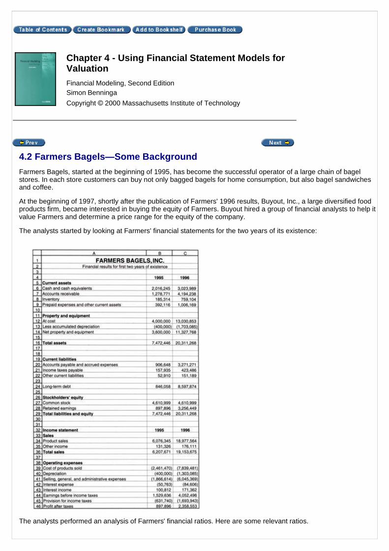
4.2 Farmers Bagels—Some BackgroundFarmers Bagels, started at the beginning of 1995, has become the successful operator of a large chain of bagelstores. In each store customers can buy not only bagged bagels for home consumption, but also bagel sandwichesand coffee.

At the beginning of 1997, shortly after the publication of Farmers' 1996 results, Buyout, Inc., a large diversified foodproducts firm, became interested in buying the equity of Farmers. Buyout hired a group of financial analysts to help itvalue Farmers and determine a price range for the equity of the company.

The analysts started by looking at Farmers' financial statements for the two years of its existence:

The analysts performed an analysis of Farmers' financial ratios. Here are some relevant ratios.


4.3 Building a Financial ModelThe analysts used the ratios derived in the preceding section (and some additional information that they gleanedfrom conversations with Farmers and Buyout) to build a financial model from which to predict the future financialperformance of Farmers. To build such a model, they had to make a lot of assumptions:

Model Assumptions

n Drop the distinction between product sales and other income, and predict only total sales. The consultantsdecided that they could not predict other income with any degree of accuracy. Their predictions for Farmers'sales are as follows:

The analysts were wary of predicting sales past 2001; as a result, we will have a terminal value problem, which isdiscussed in section 4.5.

n Cost of products sold will be 40 percent of sales.

n Selling, general, and administrative expenses will drop by 1 percent per year, from 32 percent of sales in 1996 to28 percent of sales in 2001.

n Interest expenses on debt will be 12 percent of average debt balances throughout the year, and interest incomewill be 6 percent of average balances of cash and cash equivalents throughout the year.

n Farmers Bagels' income tax rate will be 41.5 percent of its income.

n The consultants felt that a "cash cushion" would be needed for Farmers, though the size of this cushion coulddecrease as the firm grew. They predicted that cash and cash equivalents would be a declining proportion ofsales:


n Accounts receivable will remain at 22 percent of sales.

n Inventory will be rise to 5 percent of sales over the next two years and remain there.

n Prepaid expenses will drop to 5 percent of sales.

n Property and equipment at cost will drop from 70 percent of incremental sales in 1996 to 40 percent ofincremental sales in 2001. The consultants explained that this decrease would result from greater efficiency inproducing bagels.

n Depreciation will be straight line at 10 percent of sales.

n Accounts payable and accrued expenses will rise by 1 percent per year until they reach 20 percent.

n Income tax payable will remain at 25 percent of taxes owed for each year. This item represents the portion of thecurrent year's taxes that will actually be paid in the following year.

n Other current liabilities will be 1 percent of sales.

n Farmers will pay no dividends during the next five years and will raise no new equity. Therefore, debt is the"plug" in the model.

The model with results from these assumptions and predictions is given as follows.

4.3.1 Negative DebtNotice that in the pro forma statements, the long-term debt balance in 2001 is projected to be negative. The model'sconstruction explains why this result occurs: Since debt is the model "plug," when the firm produces enough cash,the debt balances will all be paid off, and the amount of debt needed to balance the liabilities against the assets willbe negative. This outcome is not aesthetic (balance sheet debt is almost invariably a positive entry), although inprinciple there is nothing wrong with this procedure: Negative debt simply represents positive amounts of cash forthe firm. In our model this projection is somewhat more problematic, not only because the interest on debt (12percent) is greater than the interest earned on cash (6 percent), but also because Farmers wants to have a certainminimal amount of cash on hand. However, the solution to this problem follows the lines laid down in section 3.7.The implementation involves the following logic:

n Farmers Bagels wants to have a certain minimum ratio of cash to sales on hand. If the total value of thisminimum cash balance plus all other assets is greater than current liabilities plus equity, then Farmers needs

debt.

n If, on the other hand,

[Cash ratio] * Sales + Accounts receivable + Inventory + Prepaid expenses + Net property and equipment − Currentliabilities − Common stock − Retained earnings < 0

then debt is set at 0. In this case

Total liabilities > Accounts receivable − Inventory − Prepaid expenses − Net property and equipment

The difference between the two sides of this inequality is the cash account (which will exceed the minimum desiredcash balances).

This procedure produces the following pro forma financial statements.


4.4 Deriving the Free Cash Flows (FCF) for Farmers BagelsAs explained in section 3.3, free cash flow (FCF) is a concept that refers to the cash produced by the businessactivities of the firm. Another way of viewing the FCF is that it is the amount of cash that the firm would produce if ithad no financial assets whatsoever—no debt and no cash or marketable securities.

The formal definition is the following:

A firm's FCF is often negative, even if it has positive profits. This tends to be true especially during periods of quickgrowth, when large amounts of new assets are needed to provide the basis from which to make new sales. It wascertainly true for Farmers during the first two years of its existence:

During its first two years of existence, Farmers Bagels produced healthy profits, but much financing was needed forincreases in net working capital (defined as the difference between current assets and current liabilities) and for thepurchase of new fixed assets. Until the growth of Farmers' sales moderates, or until the company gets larger, we canexpect this trend to continue.

The following table shows the projected free cash flows for Farmers Bagels in the next five years:

Only in 1999 was Farmers projected to produce its first positive cash flows.


Calculation of the Free Cash Flow

Profit after taxes (PAT)

Add back depreciation

Add back interest paid, net of taxes

Subtract out interest earned, net of taxes

Subtract increase in current assets except for cash and cash equivalents

Add increase in current liabilities

Subtract new fixed assets purchased (subtract change in fixed assets at cost)

4.5 Calculating Farmers' Weighted Average Cost of CapitalIn order to value Farmers Bagels, we calculate its weighted average cost of capital, defined as

where rE is the firm's cost of equity, rD is its cost of debt, TC is its marginal corporate tax rate, and D and E refer tothe market values of Farmers' equity and debt, respectively. Cost of capital calculations tend to have a lot of "noise":The cost of capital for an individual firm may be affected by random factors that are not necessarily relevant for thefuture. To avoid this problem, we calculate the average cost of capital for firms in the bagel industry, using the capitalasset pricing model (CAPM). As the next spreadsheet shows, the average asset β for firms in Farmers' industry is1.56, and the industry-average WACC is 20.43 percent:

We use the industry average WACC to value Farmers:

The present value of the 1997–2001 FCFs assumes that—on average—the cash flows occur in midyear; asdiscussed in section 3.5.2, it is therefore necessary to multiply the Excel present-value formula by (1 + WACC)0.5.This adjustment is incorporated in cell B87. When the terminal value proxies for the present value of all the FCFsbeyond the prediction horizon, the same adjustment has to be made (cell B88):

where g is the terminal growth rate.



4.6 Sensitivity AnalysisThe valuation calculations offer many opportunities for sensitivity analysis, which are easy to implement using Excel.Here we build a two-dimensional data table to calculate the value of Farmers as a function of the WACC and theterminal growth rate:

Here's the resulting data table:

Another sensitivity analysis can be done be using different proxies for the terminal value of Farmers:



4.7 ConclusionA pro forma model is an extremely useful tool for projecting cash flows and for building an integrated framework inwhich to value the firm. However, you should not be misled by the welter of numbers into thinking that the resultingvaluation is precise and immutable: The model builder uses an artistic mixture of financial theory, accountingstructure, and educated guesses to value the firm.

Exercises1. In the valuation model of section 4.5 for Farmers Bagels, build data tables that show the sensitivity of

a. The value of Farmers' equity to changes in the ratio of accounts receivable to sales.

b. The value of Farmers' equity to changes in the income tax rate.

2. The valuation model in section 4.5 assumes that increments to fixed assets at cost are a decreasing functionof sales. Change the model and assume that net fixed assets are a constant function of sales.

3. Extend the model in section 4.5 past 2001. Show that if Farmers will continue not to pay dividends, there willbe a large buildup of cash and cash equivalents. "Fix" this problem by assuming that starting in 2002,Farmers will start to pay a fixed proportion of its profits in dividends.

4. Do a sensitivity analysis of the section 4.6 valuation using the market/book (M/B) ratio. Vary the M/B ratiofrom 0.8 to 2.

5. Do a sensitivity analysis of the section 4.6 valuation using the price/earnings (P/E) ratio, varying this ratio from4 to 20.

6. Suppose that the average EBITDA ratio for the bagel industry is 8. Use this EBITDA ratio to value FarmersBagels' shares.



Chapter 5: The Financial Analysis of Leasing

5.1 IntroductionA lease is a contractual arrangement by which the owner of an asset (the lessor) rents the assets to a lessee. In thischapter we analyze leases, starting from the viewpoint of the lessee. The leases analyzed in this chapter are long-term leases, in which the asset spends most of its useful life with the lessee. In economic terms the leases weconsider in this chapter are considered by the lessees as alternatives to purchasing an asset.[1]

In the example that follows we consider a company that is faced with the choice of either purchasing or leasing apiece of equipment. We assume that the operating inflows and outflows from the equipment are not affected by itsownership—irrespective of how the asset is held (whether owned or leased) the owner/lessee will have the samesales and must bear the responsibility for maintaining the equipment. In the words of Statement 13 of the FinancialAccounting Standards Board, the lease we are considering is one that "transfers substantially all of the benefits andrisks incident to the ownership of property" to the lessor.

The analysis in this chapter concentrates exclusively on the cash flows from the lease. It is assumed that the lessorpays taxes on the income from the lease rentals and gets a tax shield on the depreciation of the asset, and that thelessee can claim the rent as an expense. The analysis implicitly assumes that the tax authorities treat the lessor asthe owner of the asset and the lessee as the user. As is explained in the appendix to this chapter, this assumption isnot trivial. In addition to the cash-flow issues of leasing there are heavy accounting issues, which are also touchedon briefly in the appendix.

[1]Thus the analysis of this chapter fits many long-term equipment leases, but not short-term leasing (car rentals, forexample).

Chapter 5 - The Financial Analysis of Leasing




5.2 A Simple ExampleThe essence of our analysis can be understood from the following simple example: A company has decided toacquire the use of a machine costing $540,000. If purchased, the machine will be depreciated on a straight-line basisto a residual value of zero. The machine's estimated life is six years, and the company's tax rate TC is 38 percent.

The company's alternative to purchasing the machine is to lease it for six years. A lessor has offered to lease themachine to the company for $130,000 annually, with the first payment to be made today and with five additionalpayments to be made at the start of each of the next five years.

One way of analyzing this problem (a misleading way, as it turns out) is to compare the present values of the cashflows to the company of leasing and of buying the asset. The company feels that the lease payment and the taxshield from depreciation are riskless. Suppose, furthermore, that the risk-free rate is 12 percent. On the basis of thefollowing calculation, the company should lease the asset.[2]

This analysis suggests that leasing the asset is preferable to buying it. However, it is misleading because it ignoresthe fact that leasing is very much like buying the asset with a loan. The financial risks are thus different when wecompare a lease (implicitly a purchase with loan financing) against a straight-forward purchase without loanfinancing. If the company is willing to lease the asset, then perhaps it should also be willing to borrow money to buythe asset. This borrowing will change the cash-flow patterns and could also produce tax benefits. Hence, our leasingdecision could change if we were to take the loan potential into account.

In the following section we present a method of analyzing leases that deals with this problem by imagining what kindof loan would produce cash flows (and hence financial risks) equivalent to those produced by the lease. This methodof lease analysis is called the equivalent-loan method.

[2]At this point we assume that the residual value of the asset at the end of its life is zero. In section 5.5 we drop thisassumption.





5.3 Leasing and Firm Financing: The Equivalent-Loan MethodThe idea behind the equivalent-loan method is to devise a hypothetical loan that is somehow equivalent to the lease.[3] It then becomes easy to see whether the lease or the purchase of an asset is preferable.

The easiest way to understand the equivalent loan method is with an example. We return to the previous example:

Rows 3–7 give the parameters of the problem. The spreadsheet then compares two after-tax cash flows, that of thelease and that of the buy. Note that we write outflows with a minus sign and inflows (such as the tax shield from thedepreciation) with a plus sign.

n The cash flow from leasing the asset is (1 − Tax rate) * Lease payment in each of years 0–5.

n The cash flow from buying the asset is the asset cost in year 0 (an outflow, hence positive) and the tax shield onthe asset's depreciation, Tax rate * Depreciation, in years 1–6 (an inflow, hence written here with a negativesign).

Line 20 of the spreadsheet shows the differential cash flow between the lease and the buy decision. This line showsthat leasing the asset, instead of buying it, results in

n A cash inflow of $459,400 in year 0. This inflow is the cash saved at time 0 by the lease.

n A cash outflow of $114,800 in years 1–5 and an outflow of $34,200 in year 6. This outflow corresponds to themarginal after-tax cost of the lease versus the buy in these years. This marginal cost has two components: theafter-tax lease payment ($80,600) and the fact that when we lease we do not get the tax shield on the asset'sdepreciation ($34,200).

Thus leasing instead of purchasing the asset is like getting a loan of $459,400 with after-tax repayments of $114,800in years 1–5 and an after-tax repayment of $34,200 in year 6. The lease, in other words, can be viewed as analternative method of financing the asset. In order to compare the lease to the buy, we should compare the cost ofthis financing with the cost of alternative financing. The internal rate of return of line 22—9.60 percent—gives us thecost of the financing implicit in the lease; this is larger than the after-tax cost of firm borrowing, since in this case(where the firm's tax rate is 38 percent and its borrowing cost is 12 percent), this cost is 7.44 percent. Thus ourconclusion: Buying is preferable to leasing.




5.3.1 Why We Decided Against the LeaseNot everyone is fully convinced by the preceding argument. We therefore present an alternative argument in thissubsection. We show that if the firm can borrow at 12 percent, it can borrow more money with the same schedule ofafter-tax repayments as that which resulted from the lease versus the buy. This hypothetical loan is shown in thefollowing table:

The table (a version of the loan tables discussed in Chapter 1) shows the principal of a hypothetical bank loanbearing a 12 percent interest rate. At the beginning of year 0 (i.e., at the time when the firm either purchases orleases the asset), for example, the firm borrows $487,443 from the bank. At the end of the year, the firm repays$137,027 to the bank, of which $58,493 is interest (since $58,493 = 12 percent * 487,443) and the remainder,$78,534, is repayment of principal. The net, after-tax, repayment in year 1—assuming full tax deductibility of theinterest payment—is (1 – 38 percent) * 58,493 + 78,534 = 114,800, which is, of course, the same after-tax differentialcash flow calculated in our original spreadsheet.

Payments in subsequent years are calculated similarly to the illustration in the preceding paragraph. At the beginningof year 6, there is still $31,832 of principal outstanding; this is fully paid off at the end of the year with an after-taxpayment of $34,200.

The point of this example? If the firm is considering leasing the asset in order to get the financing of $459,400 thatthe lease gives, it should instead borrow $487,443 from the bank at 12 percent; it can repay this larger loan with thesame after-tax cash flows as are implicit in the lease. The bottom line: Purchasing is still preferable to leasing theasset.

The loan table was constructed in the following way:

n The principal at the beginning of each of years 1–6 is the present value of the lease-versus-buy outflows,discounted at (1 − 38 percent) * 12 percent. Thus, for example,

Once the principal at the start of each year is known, it is an easy matter to construct the rest of thecolumns.

Interest = 12 percent * Principal, beginning of year

Total payment = Interest in year t + Repayment of principal in year t

After-tax payment, year t = (1 − Tax rate) * Interest + Repayment of principal

[3]This method is due to Myers, Dill, and Bautista (1976). A somewhat more accessible explanation can be found inLevy and Sarnat (1979).


5.4 The Lessor's Problem: Calculating the Highest Acceptable Lease RentalThe lessor's problem is the opposite of that of the lessee:

n The lessee has to decide whether—given a rental rate on the leased asset—it is preferable to buy the asset orlease it.

n The lessor has to decide what minimum rental rate justifies the purchase of the asset in order to lease it out.

One way of solving the lessor's problem is to turn the preceding analysis around. We use the Excel Goal Seek(Tools|Goal Seek) to get $121,047 as the lessor's minimum acceptable rental:

Here's what the Goal Seek settings look like:

If you're using Solver to do this problem, it would look like:




The symmetry between the lessee's problem and the lessor's problem suggests that if the lessee wants to lease, itwill not be profitable for the lessor to purchase the asset in order to lease it out. In some cases, however, it may bethat depreciation schedules and differences in tax rates between the lessee and the lessor make it profitable for bothto enter into a leasing arrangement. An example is given in the exercises for this chapter.

Some Peculiarities of the Excel Solver and Excel Goal Seek1. Neither of these (otherwise wonderful) Excel tools will accept a formula in the box that specifies the target.

Thus—in the present example—we would have liked to write the formula =(1-B7)*B4 in the To value boxof Goal Seek. But that technique won't work: We have to specify a numerical value (in this case, the after-tax interest rate).

2. You may have to fiddle with Tools|Options|Calculation in order to specify enough accuracy to get cellB23 to be exactly 7.44 percent. If you do not get an acceptable answer, set a higher value for the optionMaximum change.

3. Goal Seek does not remember its settings between accesses. Therefore, you will have to reenter thedata each time. (Solver, on the other hand, does remember its settings.)


5.5 Asset Residual Value and Other ConsiderationsIn the example, we have ignored the residual value of the asset—its anticipated market value at the end of the leaseterm. In a mechanical sense, it is easy to include the residual value in the calculations (but you have to be careful—see the warning after the next numerical example). Suppose, for example, you think that the asset will have a marketvalue of $100,000 in year 7; assuming that this value is fully taxed (after all, we've depreciated the asset to zerovalue over the first six years), the after-tax residual value will be (1 − Tax rate) * $100,000 = $62,000.

Not surprisingly, the possibility of realizing an extra cash flow from asset ownership makes the lease even lessattractive than before (you can see this difference by noting that the return rate in cell B24, the IRR of the differentialcash flows, has increased from 9.60 percent in our original example to 10.02 percent).

Be a bit careful here, however; the spreadsheet treats the residual value as if it has the same certainty of realizationas the depreciation tax shields and the lease rentals. This assumption can be far from the truth! There is no goodpractical solution to this problem; an ad hoc way of dealing with it might be to reduce the $100,000 by a factor thatexpresses the uncertainty about its realization. The finance technical jargon for this is "certainty-equivalence factor,"and you can find it referenced in any basic finance text.[4] The last spreadsheet snapshot in this chapter assumesthat you've decided that the certainty-equivalence factor for the residual value is 0.7:




Exercises1. Your company is considering either purchasing or leasing an asset that costs $1,000,000. The asset, if

purchased, will be depreciated on a straight-line basis over six years to a zero residual value. A leasingcompany is willing to lease the asset for $300,000 per year; the first payment on the lease is due at the timethe lease is undertaken (i.e., year 0), and the remaining five payments are due at the beginning of years 1–5.Your company has a tax rate TC = 40 percent and can borrow at 10 percent from its bank.

a. Should your company lease or purchase the asset?

b. What is the maximum lease payment it will agree to pay?

2. ABC Corporation is considering leasing an asset from XYZ Corporation. Here are the relevant facts:

Show that it will be advantageous both for ABC to lease the asset and for XYZ to purchase the asset in orderto lease it out to ABC.

3. Continuing with the same example: Find the maximum rental that ABC will pay and the minimum rental thatXYZ will accept.

4. Perform a sensitivity analysis (using Data|Table, see Chapter 26) on the certainty-equivalence factor insection 5.5, showing how the IRR of the differential cash flows varies with the CE factor.

Appendix: The Tax and Accounting Treatment of LeasesThis chapter discusses the case where the lessor retains the tax benefits of ownership; that is, the lessor is able totake the depreciation on the leased asset, and the lessee deducts the lease payments from his income as anexpense. In order for these things to happen, it is critical that the Internal Revenue Service be willing to recognize thelease as a true lease.

Although the specific IRS rules change from time to time, the principle underlying the rules remains that the lessorshould be accorded the benefits of ownership only if he bears some of the economic risks of ownership. Thisprinciple has led the IRS to develop a series of tests to determine whether or not the lessor has transferredessentially all of the ownership risks to the lessee. If this is the case, the IRS treats the "lease" arrangement as asale of the asset by the "lessor" to the "lessee." If the ownership risks have not all been transferred to the lessee,then the lease is a true lease, and the analysis of the chapter holds.

Revenue Ruling 55–540 sets out seven conditions under which a transaction will be found to be a sale rather than alease for tax purposes:

n Portions of the rental payments are specifically applicable to an equity interest to be acquired by the lessee.

n The lessee will acquire title upon payment of a stated amount of rentals.

n A substantial proportion of the asset's purchase price is paid in rentals in a relatively short period of time fromthe inception of the lease.

n The rental payments exceed a "fair" rental value.

Asset cost $1,000,000Depreciationschedule

Year1: 20%Year 2: 32%Year 3: 19.20%Year 4: 11.52%Year 5: 11.52%Year 6: 5.76%

Lease term 6 yearsLease payment $200,000 per year, at the beginning of years 0, 1, …, 5Asset residualvalue

Zero

Tax rates ABC:TC = 0% (ABC has tax-loss carryforwards that prevent it from utilizing anyadditional tax shields)XYZ: TC = 40%

n There is a bargain-purchase option; the option price is nominal in relation to the fair market value of the asset atthe time when the option can be exercised.

n Some part of the payments is designated as interest.

n The lease may be renewed at nominal rentals over the useful life of the asset.

In addition to these conditions, Revenue Ruling 55–541 deals with the relation of the lease term to the useful life ofthe asset. The ruling would seem to suggest that the transaction will be classified as a conditional sale and not as alease if the useful life of the asset is not in excess of the lease term.

One lease packager states that the IRS will generally classify a lease as a true lease if all of the following criteria aremet:

n The estimated fair market value of the leased asset at the end of the lease term will equal at least 20 percent ofthe original cost of the leased property.

n The lease term does not exceed 80 percent of the estimated useful life of the asset.

n There is no bargain-purchase option.

n The lessor's equity in the leased asset is at least 20 percent.

The Accounting Treatment of LeasesAccountants have found leases troublesome. Before the advent of Financial Accounting Standards Board Statement13 (FASB 13) in 1976, it was common for firms to leave leases off their balance sheets altogether, and to record thefact that some assets were leased only in footnotes to the financial statement. This practice created an asymmetrybetween the accounting treatment of a lease and the accounting treatment of a purchase of an asset with debt.Since the economic similarity between these two transactions is great, this asymmetric treatment is illogical.

FASB 13 attempts to solve this problem. The statement is long and complex, and it is beyond the purview of thisbook to fully present the statement's solutions. We will sketch here the solution to the problem as outlined in FASB13; the next chapter deals with FASB 13's treatment of the leveraged leases.

The basic idea behind the FASB 13 treatment of leases is that in some cases the lessee should record a leasedasset on his balance sheet, even though legally the asset belongs to another party. The cases in which this shouldhappen are those in which the economic substance of the lease transaction (as opposed to the legal fiction) is thatthe lessee effectively owns the asset. An example would be a 10-year noncancelable lease of an automobile. By thetime the car is returned to the lessor, it is likely to be practically worthless; hence, FASB 13 would require the lesseeto record the asset on his balance sheet.

Formally, FASB 13 requires the lessee to put the lease on his balance sheet (the terminology is that in this case thelease is a capital lease) if one of four criteria applies:

1. The lease transfers ownership of the property to the lessee at the end of the lease term.

2. The lease contains a bargain-purchase option, which allows the lessee to purchase the leased asset at a verylow price at the end of the lease term.

3. The lease term exceeds 75 percent of the life of the asset.

4. The present value of the lease payments (at the lessee's incremental borrowing rate) exceeds 90 percent ofthe asset's fair value.

If a lease is a capital lease under the FASB 13 rules, then the lessee records the capital lease as an asset andrecords a corresponding liability on his balance sheet. The asset is then depreciated, and the liability is amortized,over the lease term. It is as if the asset in question has been bought with 100 percent loan financing.

What does the lessor do if the lessee has to record the lease on his balance sheet? If the lessee has (in anaccounting sense) bought the asset with 100 percent loan financing, then the lessor must have (in the same sense)sold the asset with 100 percent loan financing. This is the essence of the FASB 13 treatment of the lessor.

Reconciling the Tax and Accounting Treatments of LeasesThe tax treatment and the accounting treatment of leases are very similar in spirit. It is therefore logical to expect thatwhenever a lease is classified under the FASB 13 rules as a capital lease, it should be classified by the IRS as asale. If the world were a rational place, lessees would put leases on their books only if the IRS decided to treatleases as sales.

However, the world is a funny place. It turns out to be fairly simple to keep a lease off the lessee's balance sheet,have the IRS treat it as a true lease, and still have all the parties involved feel as if they had transferred all of theeconomic benefits of ownership from the lessor to the lessee. See the references for further reading.

[4]For further references on certainty equivalents, see Brealey and Myers (1996, p. 225). However, note that neitherthis work nor the present text (nor anyone else) can tell you precisely how to calculate the certainty-equivalencefactor. It depends on your attitudes toward risk.


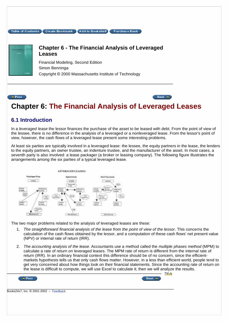
Chapter 6: The Financial Analysis of Leveraged Leases

6.1 IntroductionIn a leveraged lease the lessor finances the purchase of the asset to be leased with debt. From the point of view ofthe lessee, there is no difference in the analysis of a leveraged or a nonleveraged lease. From the lessor's point ofview, however, the cash flows of a leveraged lease present some interesting problems.

At least six parties are typically involved in a leveraged lease: the lessee, the equity partners in the lease, the lendersto the equity partners, an owner trustee, an indenture trustee, and the manufacturer of the asset. In most cases, aseventh party is also involved: a lease packager (a broker or leasing company). The following figure illustrates thearrangements among the six parties of a typical leveraged lease.

The two major problems related to the analysis of leveraged leases are these:1. The straightforward financial analysis of the lease from the point of view of the lessor. This concerns the

calculation of the cash flows obtained by the lessor, and a computation of these cash flows' net present value(NPV) or internal rate of return (IRR).

2. The accounting analysis of the lease. Accountants use a method called the multiple phases method (MPM) tocalculate a rate of return on leveraged leases. The MPM rate of return is different from the internal rate ofreturn (IRR). In an ordinary financial context this difference should be of no concern, since the efficient-markets hypothesis tells us that only cash flows matter. However, in a less than efficient world, people tend toget very concerned about how things look on their financial statements. Since the accounting rate of return onthe lease is difficult to compute, we will use Excel to calculate it; then we will analyze the results.

Chapter 6 - The Financial Analysis of LeveragedLeasesFinancial Modeling, Second EditionSimon BenningaCopyright © 2000 Massachusetts Institute of Technology


6.2 An ExampleWe can explore these issues by considering an example, roughly based on an example given in Appendix E ofFASB 13, the accounting profession's magnum opus on accounting for leases.

A leasing company is considering the purchase of an asset whose cost is $1,000,000. The asset will be purchasedwith $200,000 of the company's equity and with $800,000 of debt. The interest on the debt is 10 percent, so that theannual payment of interest and principal over the 15-year term of the debt is $105,179.[1]

The company will lease the asset out for $110,000 per year, payable at the end of each year. The lease term is 15years. The asset will be depreciated over a period of eight years, using the standard IRS depreciation schedule forassets with a seven-year life.[2] The depreciation schedule for such assets is as follows:

Because the asset will be fully depreciated at the time it is sold (year 16), the whole anticipated residual value($300,000) will be taxable. The company's tax rate is 40 percent.

These facts are summarized in the following spreadsheet, which also derives the lessor's cash flows.


Year Depreciation %1 14.282 24.493 17.494 12.55 8.926 8.927 8.928 4.48

The last column gives the cash flow to the equity owners of the asset. A typical year's cash flow for the equity owneris calculated as follows:

The explanation is as follows:

The cash flows of the typical long-lived leveraged lease areusually positive at the beginning of the lease term, andthen decline over time, turning positive again at the end, when the residual value is received. There are threereasons for this phenomenon:

1. The cash flow that stems from depreciation typically ends or falls off rapidly before the end of the lease term.The more accelerated the depreciation method, the larger will be the depreciation allowances (and hence thelarger the depreciation tax shields) at the beginning of the asset's life.

2. In the later years of the lease, the portion of the annual debt payments devoted to interest (tax deductible)falls, while the portion of the annual debt payments that constitutes a repayment of principal (not taxdeductible) rises.

3. Finally, of course, we anticipated a large cash flow from the realization of the asset's residual value at the endof the lease term.

[1]Using Excel: =PMT(10%,15,−800,000) gives 105,179.

[2]Refer to Ross, Westerfield, and Jaffee (1996), table 7.3 (p. 171). Note that by IRS rules, an asset depreciated overa seven-year life has eight years of depreciation deductions, since it is assumed that the asset is purchased inmidyear.

Item Explanation+ (1 − Tax) * Rent Equity owners get the rental from the asset, net of any taxes.+ Tax * Depreciation Equity owners get the tax shield from the depreciation of the

asset.− (1 − Tax) * Interest The interest on the debt is tax deductible.− Repayment of debt principal Repayment of debt principal is not tax deductible.+ (1 − Tax)* Residual value This item only occurs in the last year; the residual is usually

fully taxed, since the depreciation has been taken on thewhole value of the asset.

Cash flow (t) =(1 − Tax)Rent+ Tax *Depreciation(t)− (1 − Tax)Interest(t)−Principal repayment(t)

The cash flow in a typical year (excluding the residual).


6.3 Analyzing the Cash Flows by NPV or IRRWhat do we make of these cash flows? One way of viewing the cash flows (probably the best, at least in theory) is totake their net present value (NPV) at some appropriate risk-adjusted discount rate. If we analyze the cash-flowcomponents, we see that the primary riskiness stems from three sources:

1. The lessee may default on the rental.

2. Tax rates can change, affecting the tax shields from depreciation and the cash flow from the interestpayments.

3. The residual value is highly uncertain.

The following graph shows the NPV of the cash flows at various interest rates:

Note that since the cash flows are after-tax, the relevant basis for comparison is an after-tax interest rate. Forexample, suppose the lessor feels highly certain about all the cash flows and therefore wants to compare the cashflows to his loan rate of 10 percent. Then, since the lessor's tax rate is 40 percent, the appropriate discount rate forcomparison is (1 − 40 percent) * 10 percent = 6 percent; at this rate the lease cash flows have an NPV of $38,068.

Lessors are often uncomfortable with net present value. They prefer internal rate of return as a measure of theacceptability of the lease. Since the cash flows of the lease have two changes in sign, it is—in principle—possiblethat they have two IRRs. Since the IRR is the interest rate for which the NPV graph crosses the x-axis, we can useExcel to determine graphically how many IRRs there are. The following graph shows that for a very large range ofreasonable interest rates, there is only one IRR:


We are thus safe in using IRR(cash flows,0) to determine that the internal rate of return of the lease cash flows is12.46 percent.


6.4 What Does the IRR Mean?Asking what the IRR means is relevant both to an economic understanding of the meaning of the internal rate ofreturn and to the discussion in the next section of the accounting determination of the income from a leveragedlease. To illustrate the complexities, we stray for a moment from our original example to study a much simplerexample. Consider an investment of $100,000 that has positive cash flows only for the next five years.

What is the meaning of the IRR of 8.097 percent? If we think of the initial investment of $100,000 as a loan to theproject, then each cash flow is attributable to

1. Interest on the "loan principal" outstanding at the beginning of the period,

2. Repayment of this "principal."

Of course, at the end of the five years, all of the principal must be repaid. The IRR is the "rate of interest" that exactlyrepays the "loan," with its "interest payments," over the life of the project. We can see this point in the following table,which attributes each cash flow to either "income" on the "investment outstanding at the beginning of the period" orto the "repayment of the investment":

In each period, we first "charge" the investment at the beginning of the period with an "interest charge," which is theIRR. The remaining cash flow is attributed to the repayment of the investment. Thus, for example:


Investment at beginning of period 1 (i.e., the initial investment) 100,000

Note the last line in our cash-flow attribution table: At the beginning of year 5, we still have $32,378 of investmentleft; the cash flow of $35,000 for year 5 suffices exactly to pay the income of $2,622 on this investment and to repaythe investment itself. At the beginning of year 6, there is no investment left! (This result, of course, is not a miracle—it's the way we calculated the internal rate of return.)

6.4.1 Back to the Leveraged Lease ExampleWe now apply this same logic to the cash flows of the leveraged lease.

Note that—as in our simple example—the IRR of 12.46 percent successfully attributes income in such a way that thewhole of the investment is accounted for at the end of the project's life (after 16 years, for the case of the leveragedlease). However, note that there are some unusual features of the table: five of the income figures are negative, asare seven of the "repayment of investment" terms. There are two ways to understand these features:

n In "mechanical" terms, the only way to make the table work is to have some negative income numbers. Thisinterpretation, though true, is not very interesting.

n In economic terms, the negative income figures mean that in some years the project is not worth holding onto,but that it cannot be given away. As an example consider the lessor's position at the beginning of year 9. Sevenyears of negative cash flows lie ahead. Only in eight years, in year 16, will the lessor again see a positive cashflow from the lease. A rational lessor would like to give away the lease contract at this point; the present value ofthe cash flows at the beginning of year 9 at a 10 percent discount rate is −$39,333 (and this includes therealization of the residual value at the end of year 16!). But of course no rational investor would take over thecontract at the beginning of year 9 unless she were paid to do so, or unless her discount rate were negative. It isthis fact—that the lessor would have to pay someone to take the contract off her hands in year 9—that makes usattribute negative income to the project at this point.[3] In economic terms the lease at this point is worse thanvalueless; it is a burden.

As we shall see in the next section, the negative income of leveraged leases causes the accounting profession aconsiderable headache.

[3]Negative income attribution in fact starts in year 7, showing that already at this point the project has negativeeconomic value.

Cash flow for period 31,000

8.10% * Investment at beginning of period 8,097

Cash flow available for repayment of investment 22,903

Investment at beginning of period 2 = Investment at beginning of previous period −Cash flow available for repayment in period 1

100,000 − 22,903 =77,097

6.5 Accounting for Leveraged Leases: The "Multiple-Phases Method"Financial Accounting Standards Board Statement 13 (FASB 13) mandates that the lessor in a leveraged leaseallocate the cash flow from the lease between income and investment. The logical way to do so would be to use theIRR of the lease's cash flows in the way illustrated in the preceding section. But here the promulgators of FASB 13apparently ran up against the troublesome facet of human nature that hates to record a loss even if it is economicallywarranted. (The implausibility of the method for leveraged leases mandated in the statement is explained only by theassumption that lessors did not want, under any circumstances, to record economic losses that stemmed from theleases.)

The method that was devised to avoid the reporting of negative income is sometimes termed the multiple-phasesmethod (MPM). A better term might have been "bastardized IRR method."

The fact that a somewhat silly method of recognizing income is used shouldn't bother us, since foolishness isrampant in this world. However, the complexity and the opaqueness of the method have lent it respectability. (Theremust be a lesson in this!) A little debunking, in the form of an explanation, is in order.

Suppose we let the multiple-phases rate of return Q (short for quirky) be defined as follows:

6.5.1 Calculating the Multiple-Phases-Method Rate of ReturnTo calculate the MPM Rate Q, we first set up a spreadsheet similar to the one we used to illustrate the IRR in section6.4. The one difference is that we have extended the years to include year 17 (one year after the project ends). Asolution Q should give a zero investment at the beginning of year 17. The following, for example, is not a solution forQ.


Year MPM Explanation

1 The lessor's investment in the lease at the beginning of year 1 is equalto her initial investment in the lease's equity. In our example, Investment(1) = $200,000

This is the same as thecalculation of the IRR.

t The lessor's accounting income from the lease at the end of year t is If income is positive,MPM follows theattribution of income andinvestment of thestandard IRR method.Otherwise, income is setto zero.

t The lessor's investment in the lease at the beginning of any year t> 1 isdefined as Investment (t) = Investment (t − 1) −[Cash flow (t) − 1) −Income (t − 1)]

Follows IRR method

Lastyear

Cash flow(last year) = Investment(last year) * (1 + Q) Similar to IRR method.

All the formulas in this table are the same as in the case of the IRR, with the exception of the formulas in the incomecolumn. For example, the income in year 1 has the following formula:

Using the Excel Solver, we find the solution for Q. The solver (Tools|Solver) dialog box looks like this:

The target cell $D$26 is the investment at the beginning of year 17; since this is one year after the project ends, thisinvestment should be zero. When this method is applied in our case, the solution is as follows:

6.6 Comparing the MPM Rate of Return with the IRRThe MPM rate of return is widely used in the leveraged-leasing industry. How does it compare with the IRR?

n In general, the MPM rate of return is less than or equal to the IRR. The two will be equal if all the lease's cashflows are positive. Otherwise the MPM rate of return is less than the IRR.

n If the MPM rate of return is less than the IRR, then at some point the IRR will attribute negative income to thelease, whereas the MPM will attribute zero income to the lease.

Graphically, for the specific example of this chapter, we have

Exercises1. Reconsider the leveraged-leasing example in this chapter. Show that if depreciation is straight line over 15

years, then the MPM rate of return is equal to the IRR. Explain.

2. In the leveraged-lease example of section 6.6, find the lowest lease rental so that the MPM is equal to the IRR(assume the original depreciation schedule).



financial modeling, second edition part1

Economy & Finance

open financial modeling

financial statementsimulation

financial statement

standard financial models

common financial models

editionfinancial modeling

prefacefinancial modeling

editionsimon benningacopyright