financial speculation in energy and agriculture futures markets: a
TRANSCRIPT
1
Matteo Manera,a* Marcella Nicolini,b and Ilaria Vignati c
Financial speculation in energy and agriculture futures markets:
A multivariate GARCH approach Abstract: This paper analyses futures prices of four energy commodities (crude oil, heating oil, gasoline and natural gas) and five agricultural commodities (corn, oats, soybean oil, soybeans and wheat), over the period 1986-2010. Using DCC multivariate GARCH models, it provides new evidence on four research questions: 1) Are macroeconomic factors relevant in explaining returns of energy and non-energy commodities? 2) Is financial speculation significantly related to returns in futures markets? 3) Are there significant relationships among returns, either in their mean or variance, across different markets? 4) Is speculation in one market affecting returns in other markets? Results suggest that the S&P 500 index and the exchange rate significantly affect returns. Financial speculation, proxied by Working’s T index, is poorly significant in modelling returns of commodities. Moreover, spillovers between commodities are present and the conditional correlations among energy and agricultural commodities display a spike around 2008. JEL Codes: C32; G13; Q11; Q43. Keywords: Energy; Agricultural commodities; Futures markets; Financial speculation; Multivariate GARCH. __________ a University of Milan-Bicocca, Milan and Fondazione Eni Enrico Mattei, Milan. Email: [email protected] b University of Pavia, Pavia and Fondazione Eni Enrico Mattei, Milan. Email: [email protected] c Fondazione Eni Enrico Mattei, Milan. Email: [email protected] * Corresponding author.
A previous version of this paper has been presented at the FEEM International Conference on “Financial Speculation in the Oil Market and the Determinants of the Oil Price”, held in Milan, 12-13 January 2012. We would like to thank seminar participants at FEEM, University of Milan-Bicocca and University of Pavia for helpful comments.
2
1. Introduction
The last decades have witnessed a number of changes in commodities futures markets. The oil
market has continuously grown, becoming the world's biggest commodity market and turning from
a primarily physical product activity into a sophisticated financial market (Chang et al. 2011). The
increasing presence of hedgers, as well as speculators, has led to allegations that speculation drives
crude oil prices, and speculators, index funds and hedge funds have been responsible for the
increase in energy and food prices from 2004 onwards (Masters 2008). The literature however has
provided, so far, little empirical evidence in support of this claim.
Speculators have historically been present in non-energy commodities futures markets as well: it is
therefore reasonable, while testing the role of speculators and any possible impact on commodities’
returns, to extend the analysis to both energy and non-energy commodities.
Moreover, the common behaviour displayed by energy and non-energy commodities prices in
recent times, characterized by a steep rise around year 2008 which has been followed by a sharp
decrease during the “great recession”, has posed the question of the linkage between these markets,
and the spillovers that may be present.
This paper contributes to the existing literature by shedding some light on several compelling
issues. More precisely, it focusses on four research questions. First, are macroeconomic factors
relevant in explaining returns of energy and non-energy commodities? Second, is financial
speculation significantly related to returns in futures markets? Third, are there significant
relationships among returns, either in their mean or variance, across different markets? Finally, is
speculation in one market affecting returns in other markets? Or, in other words, are there spillovers
across markets in speculation?
Our empirical exercise considers weekly data over the time period 1986:3 to 2010:52. We collect
data on returns of four energy commodities (gasoline, heating oil, natural gas and crude oil) and
four non-energy commodities (corn, oats, soybeans and wheat). Additionally, we include in our
analysis a biofuel, soybean oil, to investigate if the relationship among the latter and energy
commodities is stronger than what can be found between energy and food commodities. We
consider a generalized autoregressive conditional heteroskedasticity (GARCH) model to estimate
commodities’ returns: we first discuss an univariate analysis, where returns are explained by
macroeconomic variables and a measure of speculation. Then, we present multivariate GARCH
models to investigate the presence of spillovers across commodities.
Our results suggest that macroeconomic variables are relevant in explaining commodities’ returns,
more precisely the Standard & Poor’s (S&P) 500 index has a positive and significant coefficient,
3
while the multilateral exchange rate has a negative effect, as expected. As concerns the second
research question, we observe that speculation, measured by the Working’s T index, does not seem
to significantly affect returns. As for the third issue, we observe that returns of other commodities
are generally not significant in the mean equations (with the exception of natural gas and crude oil
in the returns of other energy commodities). We find however that the dynamic conditional
correlations among commodities are time varying and higher in recent years. Interestingly,
correlations between soybean oil and energy commodities, as well as correlations between
agricultural commodities and a factor of energy ones, present a spike around 2008. Finally, as
speculation is generally poorly significant, we do not detect a relevant impact on other markets’
returns.
The remainder of this paper is structured as follows. Section 2 discusses the debate on the impact
of speculation in futures markets and the presence of spillovers across commodities. Section 3
presents the data and some descriptive statistics. Section 4 describes the econometric model while
Section 5 presents the results. Finally, Section 6 concludes.
2. Literature review
Some commentators (Frankel 2008a, Mitchell 2008, Verleger 2009, Smith 2009) suggest that the
causes of price increases have to be identified in economic fundamentals as low interest rates in the
USA, which forced to look for other investment opportunities. Another factor is the rapid economic
growth worldwide, especially in China and India, which has been accompanied by growing demand
for food commodities. Instability among oil producers, especially in the Middle East, and therefore
uncertainty in the supply of oil has to be accounted for as well. Finally, misguided ethanol subsidies
have increased biofuel production and might have affected prices. Baffes and Haniotis (2010) add
to the latter argument claiming that the future path of commodities prices is uncertain due to the
strict relationship between energy and non-energy prices. In particular, this relationship has
increased considerably in the recent boom, indicating that events and policy changes happening in
one market affect other markets. Gilbert (2010) finds that, in the last years, oil prices have had more
influence on food ones. He claims however that this is the result of common causation rather than of
a direct causal link.
More recently, several researchers and analysts suggested that the increasing presence of
speculators in commodity future markets could explain the spike in prices in the 2007-2008 period
(see, among many, Eckaus 2008, Masters 2008, Soros 2008). Indeed, Medlock III and Jaffe (2009)
show that non-commercial agents in 2009 represented about 50% of total open interest in the oil
4
market, compared to about 20% prior to 2002. Moreover, the open interest held by speculators
moved from a lagging indicator of price to a leading indicator around January 2006, suggesting a
possible cause in oil prices increase. Khan (2009) argues that speculation played a role as the price
of crude oil and the price of gold, which used to move together until 2000, display a gap from 2002
onwards. Robles et al. (2009) find some evidence that speculative activity Granger-causes current
commodity prices of wheat, maize, soybeans and rice. Du et al. (2011) show that scalping and
speculation affect positively crude oil price volatility. Moreover, after 2006, they find that the oil
price shock has triggered price changes in corn and wheat markets, potentially because of an
increase in ethanol production.
Other authors instead do not find a statistically significant relationship between commodity prices
and index funds, which are held responsible for speculation. Index Investment Data (IID) have been
made available by CFTC from December 2007. Using these data Irwin and Sanders (2012) find
little evidence that IID positions influence returns or volatility in 19 commodity futures markets.
Authors interested in analysing the previous period proxied index funds activity using data on swap
dealers. Empirical tests provide no evidence that position changes by any trader group influence
price changes in both energy and non-energy commodities futures markets (Brunetti and
Büyükşahin 2009, Stoll and Whaley 2010, Büyükşahin and Harris 2011, Bastianin et al. 2012).
Sanders et al. (2010) study agricultural futures markets over the period 1995-2008 and show that the
Working’s T (1960) index, traditionally adopted to measure excess speculation (see Section 3 for a
formal definition), has remained stable or below historical levels in recent years. However, they
suggest that this result might be due to the nature of the index itself: the recent rise in long
speculative positions has been paralleled by an increase in short hedging, thus implying an overall
decrease in the Working’s T index. Till (2009) reaches the same conclusion for oil futures market
over the period 2006-2009.
Other authors suggest that the crude oil price spike and collapse in 2007-08, while being mainly
driven by increasing world demand, can not be explained by macroeconomic factors only and
suggest that speculation played a role (Kaufmann and Ulman 2009, Kaufmann 2011). We follow
this approach, and in the subsequent econometric analysis we investigate the role of macroeconomic
variables and speculation on futures’ returns.
The asset pricing literature provides empirical evidence of the ability of few macroeconomic
variables to forecast returns on commodities futures. The first is the return on the 90-day Treasury
bill, which represents the short-term discount rate free of a risk premium. The T-bill tends to be
lower during economic recessions and higher during periods of growth. Thus, it is expected to be
negatively correlated with real economic output growth. A negative relationship between real
5
commodity prices and real interest rates has been confirmed empirically (Frankel 2008b). The
second variable is the equity dividend yield: futures commodity prices are expected to reflect the
systemic risk embedded within the evolution of stock market conditions (Chevallier 2009). A third
variable is the “junk bond premium”, which is the premium on long-term corporate bonds rated
BAA by Moody’s over the AAA rated ones. This difference represents the monetary compensation
for risk. Recent works on petroleum futures returns and carbon futures returns (Sadorsky 2002,
Chevallier 2009) find however that these macroeconomic risk variables are poorly significant.
Finally, exchange rates are thought to be closely related to commodities futures prices, although the
direction of the causality among these variables is still debated. Indeed, Chen et al. (2010) show that
exchange rates have robust forecasting power over global commodity prices and that commodity
prices Granger-cause exchange rates in-sample.1
Another issue we tackle with the present econometric exercise is the relationship among
commodities prices and price changes. The literature has largely debated on this. Several authors
find cointegration among commodity prices (see among many Malliaris and Urrutia 1996,
Chaudhuri 2001, Natanelov et al. 2011).
Pindyck and Rotemberg (1990) analyze monthly returns of 7 commodities (wheat, cotton, copper,
gold, crude oil, lumber and cocoa) from 1960 to 1985. The commodities are chosen to be neither
substitutes nor complements, neither co-produced and neither inputs for others’ production and they
are thus expected to be uncorrelated. However, the authors find that the residuals of a regression of
these commodities’ prices on macroeconomic variables are highly correlated, meaning that prices
move together even after accounting for a set of macroeconomic variables. This “excess co-
movement” is possibly explained by the so called “herd” behaviour of financial traders.
Subsequently, several papers have challenged the excess co-movement hypothesis (Leybourne et al.
1994, Deb et al. 1996, Ai et al. 2006).
More recently the literature has concentrated on possible linkages between energy and non-energy
commodities. Indeed, crude oil is an important input in agricultural production, either in the form of
diesel, fertilizers or pesticides. Baffes (2007) measures the effect of crude oil prices on the prices of
35 internationally traded primary commodities for the 1960–2005 period, finding that the pass-
through of crude oil price changes to the overall non-energy commodity index is 0.16: a 10%
increase in the price of crude oil brings a 1.6% increase in the non-energy commodity prices.
Extending the sample up to 2008 Baffes (2010) finds that a 10% increase in energy prices brings a
1 Given the weekly frequency of data adopted in the econometric exercise we are not able to include other macroeconomic controls, such as industrial production or unemployment rate (which are available a monthly frequency).
6
2.8% increase in non-energy prices, suggesting that the 2008 financial crisis has strengthened the
relationship between energy and non-energy prices.
Researchers have focussed recently also on a specific class of commodities, biofules, and on the
possible linkages between biofuels and other food commodities. Natanelov et al. (2011) show a lack
of cointegration between corn and crude oil price between mid 2004 and July 2006, which is due to
policy interventions on biofules. However, after surpassing a certain threshold in crude oil price the
two series are cointegrated. Ciaian and Kancs (2011) show that the interdependencies among crude
oil and agricultural commodities (included corn and soybean) are increasing over time, while Du
and McPhail (2012) find that after 2008 ethanol, gasoline, and corn prices are more closely linked.
3. Data description
We collect data on futures prices for four energy commodities (light sweet crude oil, heating oil,
gasoline and natural gas) and five agricultural commodities (corn, oats, soybean oil, soybeans and
wheat). All the energy commodities are traded on the New York Mercantile Exchange (NYMEX),
while the agricultural ones are traded on Chicago Board of Trade (corn, oats, soybean oil and
soybeans) and Kansas City Board of Trade (wheat). Daily data are retrieved from Datastream and
turned into weekly averages of futures prices2 for each commodity. Indeed, data necessary to build
the speculation index are provided by the Commitments of Traders (COT) reports of U.S.
Commodity Futures Trading Commission (CFTC) on a weekly basis, thus we have to adopt this
data frequency.3 CFTC collects every week the open interest for specific categories of traders:
commercial (hedgers)4 and non-commercial (speculators and arbitrageurs),5 distinguishing between
short and long positions. The period considered spans from 1986:3 to 2010:52.6
2 We use the continuous futures price series, calculated by Thomson Financial. They start at the nearest contract month which forms the first values for the continuous series and switch over on 1st day of new trading month. 3 Notice that daily data exist, but are not publicly available. 4 Commercial agents are also active in the spot market. In this category CFTC includes producers, merchants, processors and users, i.e. who use futures markets to manage or hedge risks associated with the physical activity of commodities, and swap dealers, i.e. all the agents who use these markets to manage or hedge the risk associated with swap transactions. 5 Non-commercial agents are in futures markets to make profits from selling and buying futures contracts. In this category CFTC includes money managers, i.e. a category which includes a registered commodity trading advisor (CTA), a registered commodity pool operator (CPO) or an unregistered fund identified by CFTC, and other reportables, i.e. any trader that is not identified in the previous categories. 6 From January 1986 to September 1992 CFTC reports data with bi-monthly frequency. Missing data are replaced by the average between the previous and the following observation. As a robustness check, we estimate the models in the period running from September 1992 to December 2010. Results are unaffected. These estimates are reported in the statistical appendix, available from the authors upon request.
7
The data collected allow to calculate the Working’s T index, which is a measure of speculative
activity that proxies the excess of speculation relative to hedging activity. This index is calculated
as the ratio of non-commercial positions to total commercial positions:
<+
+
≥+
+
HLHSifHLHS
SL
HLHSifHLHS
SS
1
1 (1)
where SS is speculation short, SL is speculation long, HS is hedging short and HL is hedging long.
It should be noted that the calculation of the Working’s T index crucially depends on the
classification of the market operators between hedgers and speculators. CFTC also provides data for
“Non Reportable” agents,7 which are not classified into any of the two categories. However, open
interest held by these subjects should be included in the computation of the index. Several rules to
treat them are at hand. One could consider them as being all hedgers or, more likely, all speculators.
Indeed, hedgers are generally known by CFTC and are less likely to be among non reportables. We
follow an intermediate approach, assuming that 70% of them are speculators and 30% are hedgers.
However, we calculate the speculation index also in the two “extreme” hypotheses and perform the
econometric exercise with these variables.8
To control for macroeconomic factors we collect daily (5 days) data, which we turn into weekly
averages, on Moody’s AAA and BAA corporate bond yield, 3-month Treasury bill, S&P 500 index
and a weighted exchange rate index of the U.S. dollar against a subset of broad index currencies
outside U.S. for the period 01/02/1986 - 12/31/2010 from the Federal Reserve Economic Data
(FRED) provided by the Federal Reserve of St. Louis.9
Descriptive statistics of the variables are reported in Table 1. Futures prices and macroeconomic
variables contain a unit root, as the Augmented Dickey-Fuller (ADF) test statistics does not reject
the null hypothesis for almost all series in the dataset. Therefore, for each commodity we consider
7 CFTC defines this category as follows: “The long and short open interest shown as "Non Reportable Positions" is derived by subtracting total long and short "Reportable Positions" from the total open interest. Accordingly, for "Non Reportable Positions", the number of traders involved and the commercial/non-commercial classification of each trader are unknown.” (see http://www.cftc.gov/MarketReports/CommitmentsofTraders/ExplanatoryNotes/index.htm) Notice that threshold levels for non-reportables have changed over time. As long as non-reportables are included in the computation of the Working’s T index and our results using different rules to attribute non-reportables (see more infra) to the different trading categories are robust, we might expect that the change in thresholds does not impair our results. 8 Results are similar using alternative definitions of the Working’s T index. They can be found in the statistical appendix available from the authors upon request. 9 The trade weighted exchange index is defined as a weighted average of the foreign exchange value of the U.S. dollar against a subset of the broad index currencies that circulate widely outside the country of issue. Major currency index includes the Euro Area, Canada, Japan, United Kingdom, Switzerland, Australia, and Sweden. According to this definition, a decrease of the index corresponds to a depreciation of the U.S. dollar.
8
the return itr , which is defined as )/log( 1−itit PP , where itP and 1−itP are the prices of commodity i at
weeks t and t-1, respectively. This transformation allows to obtain stationarity, as shown in the
second panel of Table 1.
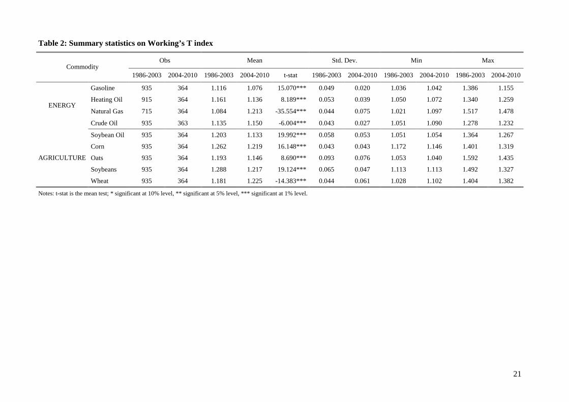
The third panel shows that Working’s T index ranges from mean values of 10.5% (in gasoline) to
26.8% (in soybeans) and, in the entire sample, it reaches maximum values of around more than 50%
(in natural gas and oats). The index is stationary in levels and therefore is not transformed.
However, the long time span considered in our sample may, on average, conceal the role of
speculation in recent times. We report summary statistics for two different periods: 1986-2003 and
2004-2010 to inspect if any change of this index occurred across different commodities over time.
The choice is driven by the consideration that the sharp increase in oil prices is generally
acknowledged to begin in 2004 (Smith 2009): in this year the oil demand exceptionally reaches a
record level of almost three millions barrels a day10 and the S&P GSCI (Goldman Sachs
Commodity Index) sharply accelerates. Results are reported in Table 2. First, we observe that in the
1986-2003 period energy commodities display lower mean values than non-energy ones. Second,
mean values are generally lower in the 2004-2010 period, with the notable exception of natural gas,
crude oil and wheat: excess speculation has increased in recent times for these commodities. The
tests of the equality of means reported in Table 2 suggest that these differences are statistically
significant.
The contemporaneous rise in agricultural and energy prices poses the question of the linkages
between these markets and the spillovers that may take place: preliminary evidence is provided by
the correlations between the variables employed in the estimation.11 The highest correlations are
those between returns of energy commodities (generally higher that 0.7), while soybean oil,
notwithstanding its widespread use as fuel, is poorly correlated with them. Correlations between
returns and Working’s T indexes are in almost all cases not significant, suggesting that the
relationship linking these variables is weak and anticipating the result found in the econometric
analysis that speculation is not relevant in explaining futures returns. Correlations between
speculation indexes are generally not large and mixed in sign.
4. The econometric specification
We aim at modelling the returns of commodities’ futures prices. As a preliminary step, we test for
stationarity of all the series, and take the log difference if necessary (see Table 1).
10 See U.S. Energy Information Administration (2008). 11 The correlation matrix is not reported but is available in the statistical appendix.
9
Then, we estimate the following equation:
0 1 2 3 4 5_ _ _ & _it t t t t it itr int rate junk bond yield S P exc rate WTα α α α α α ε= + + + + + + (2)
where the dependent variable is the return in commodity market i at time t. The macroeconomic
context is summarized by the returns of 3-month treasury bills (int_ratet), the junk bond yield, the
returns of the S&P 500 index (S&Pt) and the exchange rate between U.S. dollar and other
currencies, and the speculation present in markets, represented by the Working’s T (WTit) for the
market i at time t. We consider nine markets and the time period spans from 1986:3 to 2010:52.12
We first estimate the model with ordinary least squares (OLS) and test for autoregressive
conditional heteroskedasticity (ARCH) effects in the residuals. If such effects are present, we revert
to a generalized conditional heteroskedasticity (GARCH) model. If the GARCH term is statistically
significant, we opt for a GARCH(1,1) model, controlling that the second moment and log moment
conditions are respected. We also test for autocorrelation in the residuals and include an auto
regressive term if necessary.
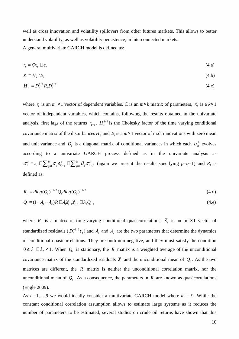
As will be shown in the next section, the GARCH(1,1) model with an AR(1) term is the preferred
specification to model the returns. Therefore, we end up estimating a model where the conditional
mean equation is:
0 1 2 3 4 5 6 1_ _ _ & _it t t t t it it itr int rate junk bond yield S P exc rate WT rγ γ γ γ γ γ γ ε−= + + + + + + + (3.a)
and the conditional variance is defined as:
2
1
2
1
2jit
q
j jjit
p
j jiitiis −=−= ∑∑ ++= σβεασ (3.b)
where the variance 2itσ of the regression model’s disturbances is a linear function of lagged values
of the squared regression disturbances and of its past value: p defines the order of the ARCH term,
and q of the GARCH term. In the econometric exercise, we estimate a model where p=q=1.
The univariate analysis is however limited in its scope: the common trend in futures prices suggests
that a multivariate approach should be implemented to investigate the presence of spillovers, both in
the mean and in the variance equation. Indeed, a multivariate-GARCH model captures the effects
on current volatility of own innovation and lagged volatility shock originated in a given market, as
12 For heating oil data are available from 1986:22, for natural gas from 1990:14.
10
well as cross innovation and volatility spillovers from other futures markets. This allows to better
understand volatility, as well as volatility persistence, in interconnected markets.
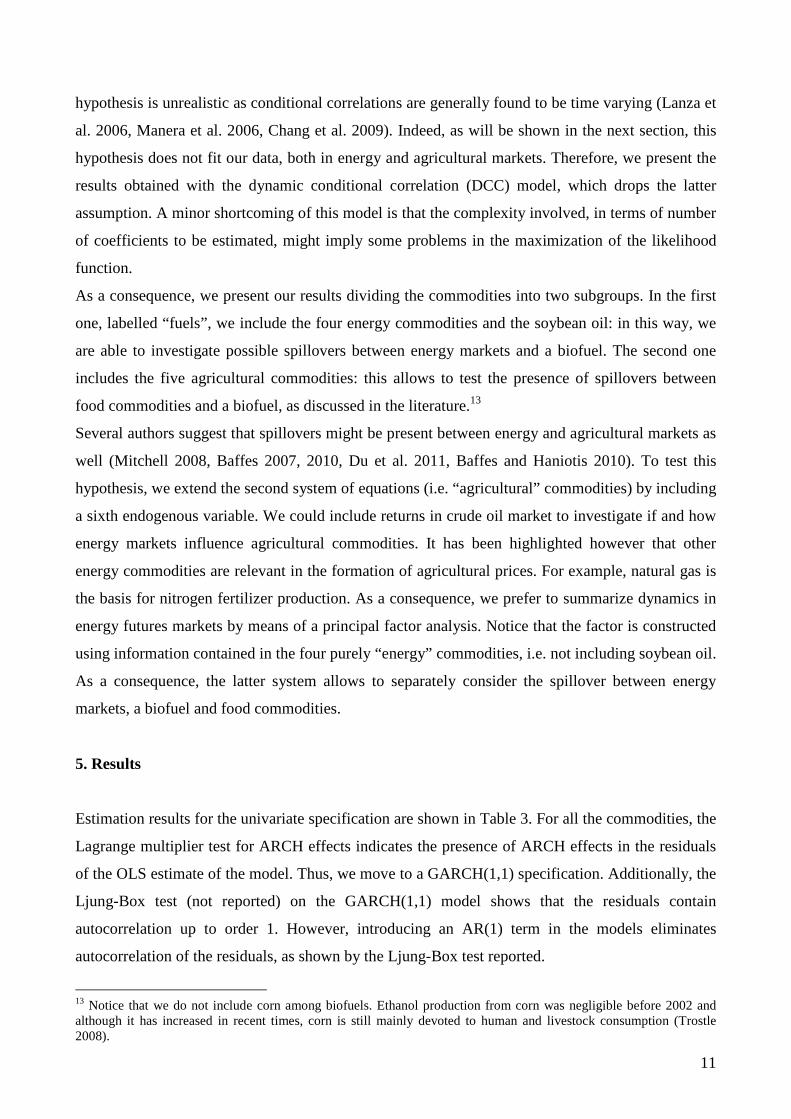
A general multivariate GARCH model is defined as:
ttt Cxr ε+= (4.a)
ttt H υε 2/1= (4.b)
2/12/1tttt DRDH = (4.c)
where tr is an m ×1 vector of dependent variables, C is an m×k matrix of parameters, tx is a k×1
vector of independent variables, which contains, following the results obtained in the univariate
analysis, first lags of the returns 1−tr , 2/1tH is the Cholesky factor of the time varying conditional
covariance matrix of the disturbancestH and tυ is a m×1 vector of i.i.d. innovations with zero mean
and unit variance and tD is a diagonal matrix of conditional variances in which each 2itσ evolves
according to a univariate GARCH process defined as in the univariate analysis as
2
1
2
1
2jit
q
j jjit
p
j jiitiis −=−= ∑∑ ++= σβεασ (again we present the results specifying p=q=1) and Rt is
defined as:
2/12/1 )()( −−= tttt QdiagQQdiagR (4.d)
12'
11121~~)1( −−− ++−−= tttt QRQ λεελλλ (4.e)
where tR is a matrix of time-varying conditional quasicorrelations, tε~ is an m ×1 vector of
standardized residuals ( ttD ε2/1− ) and 1λ and 2λ are the two parameters that determine the dynamics
of conditional quasicorrelations. They are both non-negative, and they must satisfy the condition
10 21 <+≤ λλ . When tQ is stationary, the R matrix is a weighted average of the unconditional
covariance matrix of the standardized residuals tε~ and the unconditional mean of tQ . As the two
matrices are different, the R matrix is neither the unconditional correlation matrix, nor the
unconditional mean of tQ . As a consequence, the parameters in R are known as quasicorrelations
(Engle 2009).
As i =1,…,9 we would ideally consider a multivariate GARCH model where m = 9. While the
constant conditional correlation assumption allows to estimate large systems as it reduces the
number of parameters to be estimated, several studies on crude oil returns have shown that this
11
hypothesis is unrealistic as conditional correlations are generally found to be time varying (Lanza et
al. 2006, Manera et al. 2006, Chang et al. 2009). Indeed, as will be shown in the next section, this
hypothesis does not fit our data, both in energy and agricultural markets. Therefore, we present the
results obtained with the dynamic conditional correlation (DCC) model, which drops the latter
assumption. A minor shortcoming of this model is that the complexity involved, in terms of number
of coefficients to be estimated, might imply some problems in the maximization of the likelihood
function.
As a consequence, we present our results dividing the commodities into two subgroups. In the first
one, labelled “fuels”, we include the four energy commodities and the soybean oil: in this way, we
are able to investigate possible spillovers between energy markets and a biofuel. The second one
includes the five agricultural commodities: this allows to test the presence of spillovers between
food commodities and a biofuel, as discussed in the literature.13
Several authors suggest that spillovers might be present between energy and agricultural markets as
well (Mitchell 2008, Baffes 2007, 2010, Du et al. 2011, Baffes and Haniotis 2010). To test this
hypothesis, we extend the second system of equations (i.e. “agricultural” commodities) by including
a sixth endogenous variable. We could include returns in crude oil market to investigate if and how
energy markets influence agricultural commodities. It has been highlighted however that other
energy commodities are relevant in the formation of agricultural prices. For example, natural gas is
the basis for nitrogen fertilizer production. As a consequence, we prefer to summarize dynamics in
energy futures markets by means of a principal factor analysis. Notice that the factor is constructed
using information contained in the four purely “energy” commodities, i.e. not including soybean oil.
As a consequence, the latter system allows to separately consider the spillover between energy
markets, a biofuel and food commodities.
5. Results
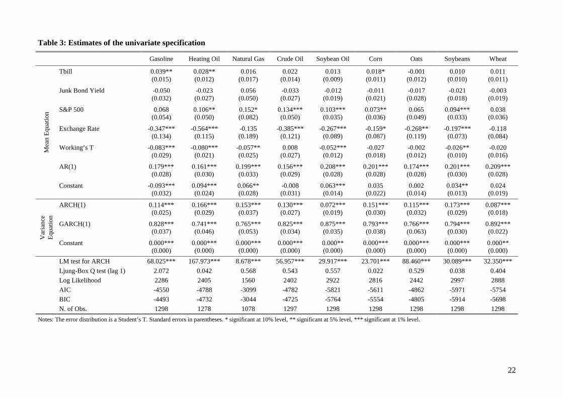
Estimation results for the univariate specification are shown in Table 3. For all the commodities, the
Lagrange multiplier test for ARCH effects indicates the presence of ARCH effects in the residuals
of the OLS estimate of the model. Thus, we move to a GARCH(1,1) specification. Additionally, the
Ljung-Box test (not reported) on the GARCH(1,1) model shows that the residuals contain
autocorrelation up to order 1. However, introducing an AR(1) term in the models eliminates
autocorrelation of the residuals, as shown by the Ljung-Box test reported.
13 Notice that we do not include corn among biofuels. Ethanol production from corn was negligible before 2002 and although it has increased in recent times, corn is still mainly devoted to human and livestock consumption (Trostle 2008).

12
The speculation index is negative or not significant. This result contrasts with claims that
speculation has affected returns in a positive way. A negative sign implies that an increase in excess
speculations corresponds to a decrease in returns.
As for the macroeconomic controls, we observe that the S&P 500 index is positive and generally
significant, and that the exchange rate is negative and generally significant, suggesting that a
depreciation of U.S. dollar compared to other currencies increases futures prices and is thus
correlated with positive returns. As expected, the ARCH (α ) and GARCH (β ) terms are always
statistically significant: the ARCH estimates are generally small (between 0.072 for soybean oil and
0.173 for soybeans) and the GARCH estimates are generally high and close to one (between 0.741
for heating oil and 0.892 for wheat). This indicates a near long memory process: a shock in the
volatility series impacts on futures volatility over a long horizon.14 Notice that our results are robust
to alternative econometric specifications, such as GARCH-in-mean, exponential GARCH and
threshold GARCH.15
To analyze the spillovers between different commodities and the linkages between different futures
markets we move to a system where the returns are jointly estimated, allowing for conditional
variances. Additionally, we can check if the speculation index of one commodity influences returns
of other ones.
Starting from a GARCH(1,1)-AR(1) specification that is supported for all commodities in the
univariate case, we consider a DCC multivariate GARCH. This model is preferred to the CCC
specification, as the conditional correlations obtained are clearly not constant over time (more
infra).16 In each equation the returns of each commodity are regressed on the macroeconomics
controls, on the lagged dependent variable17 and on the lagged returns of the other commodities.
Finally, we include among the regressors the own speculative index as well as the Working’s T of
all the other commodities, to investigate if speculation in one market is significant in other markets.
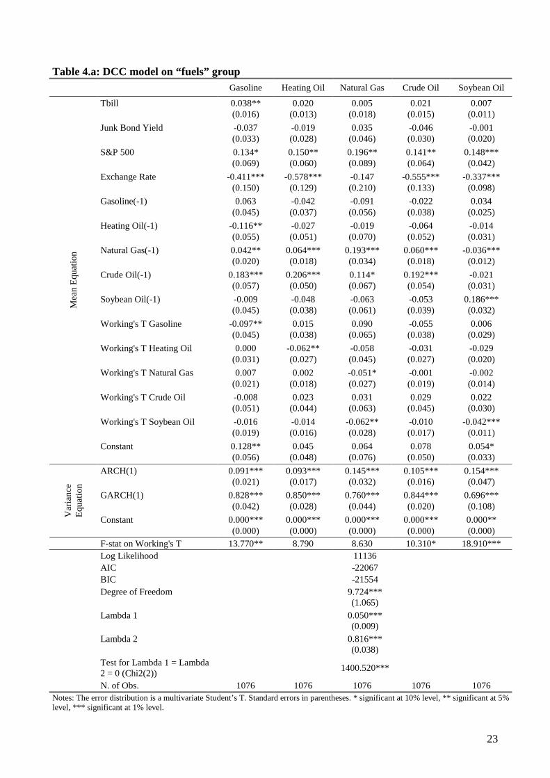
The results for the group of “fuels” commodities are presented in Tables 4.a and 4.b. Table 4.a
reports the results for the mean and variance equations. Among macroeconomic variables, the S&P
index is always positive and significant and the exchange rate is generally negative and significant.
We observe, with the exception of gasoline and heating oil, that lagged values of the dependent
variable are positive and significant, suggesting persistence in returns. Moreover, lagged returns in
crude oil and natural gas positively affect returns of the other commodities. The estimates suggest
14 As 1<+ βα for all commodities, the second moment and log-moment conditions are satisfied in all markets, and
this is a sufficient condition for consistency and asymptotic normality of the QMLE estimator (McAleer at al. 2007). 15 A summary of results using alternative specifications is available in the statistical appendix. 16 The results obtained with a CCC specification for the mean equation are very similar to the DCC ones. Therefore, they are not reported but are available in the statistical appendix. 17 We include only one lag as the univariate case supports an AR(1) model.
13
that speculation is widely not significant: the Working’s T index in own market is generally
negative, confirming the results obtained in the univariate analysis. The ARCH (α ) and GARCH
( β ) terms are always positive and statistically significant and their sum is smaller than one. Again,
the ARCH estimates are small and the GARCH estimates are generally high, confirming the
presence of a near long memory process. We estimate the models assuming a multivariate Student’s
T distribution for the error terms. The degrees of freedom of the distribution are estimated and
reported at the bottom of Table 4.a. The DCC model reduces to the CCC if the λ parameters are
both equal to zero: we test the null hypothesis that 021 == λλ and the test strongly rejects the null,
thus supporting the dynamic specification. As concerns the time-varying conditional correlations,
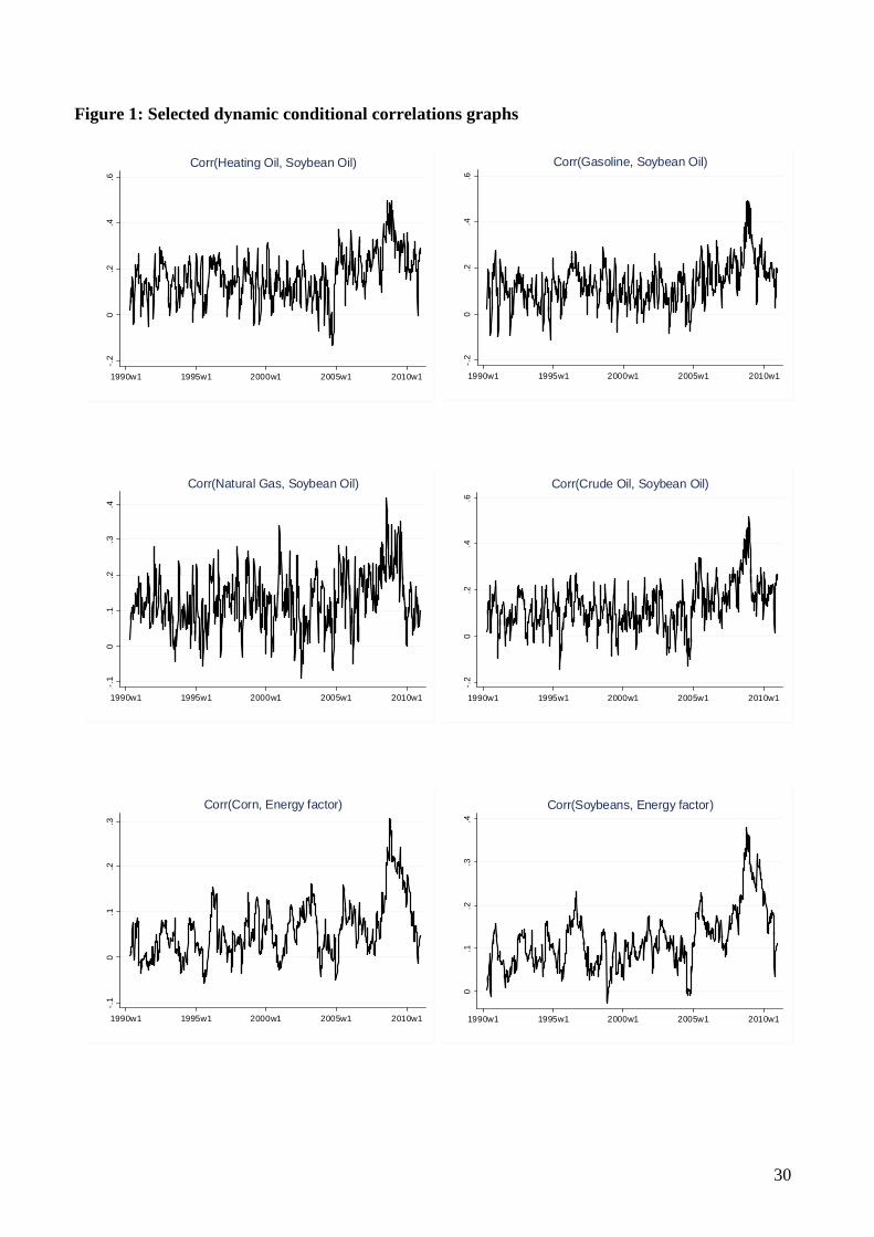
we find that correlations between soybean oil and the other energy commodities present high values
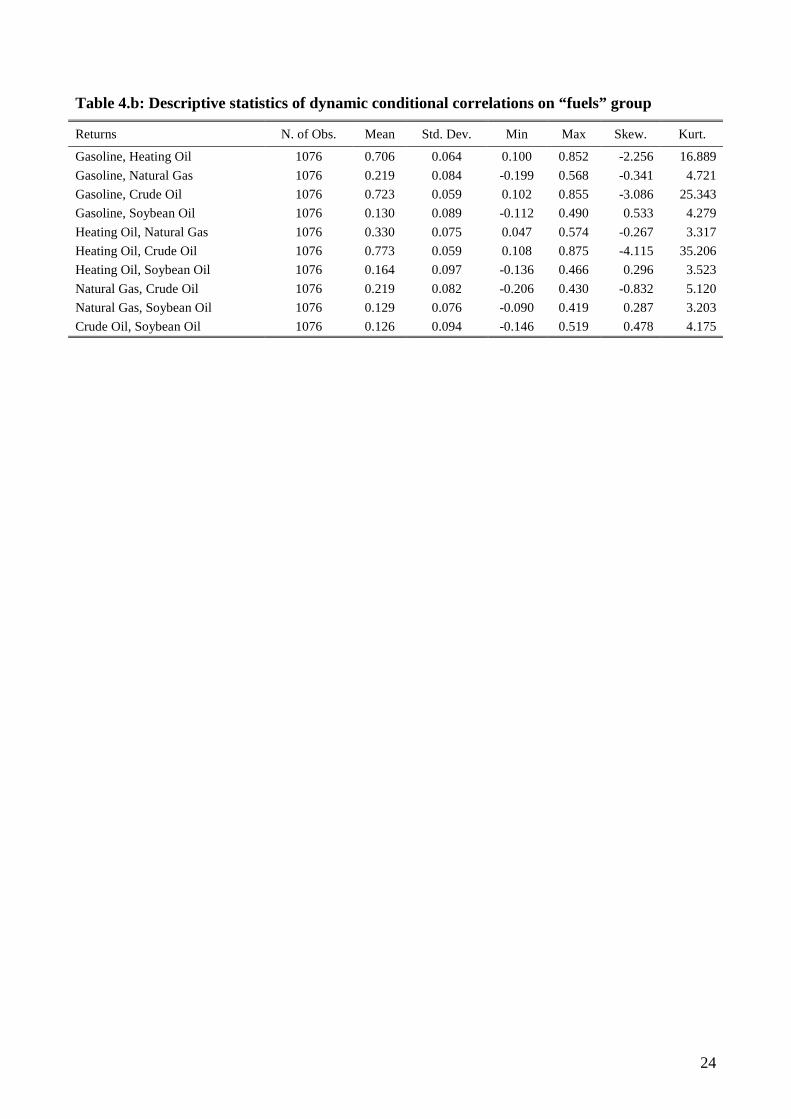
around the year 2008, i.e. in the peak period of prices (see Figure 1).18 Descriptive statistics on the
conditional correlations are reported in Table 4.b: the highest mean value observed is between
heating oil and crude oil (0.773) followed by the one between gasoline and crude oil (0.723) and
between gasoline and heating oil (0.706). The lowest mean values are those related to soybean oil.19
Besides, all the correlations vary dramatically displaying also negative values and having a large
range of variation. For example, if we consider the correlation between heating oil and crude oil, a
maximum value of 0.875 means that, on the corresponding week (13th week of 1998), heating oil
and crude oil returns would have brought almost the same risk. On the contrary, a minimum value
of -0.206 (50th week of 2000) between natural gas and crude oil means that shocks to these two
commodities are not perfect substitutes in terms of risk.
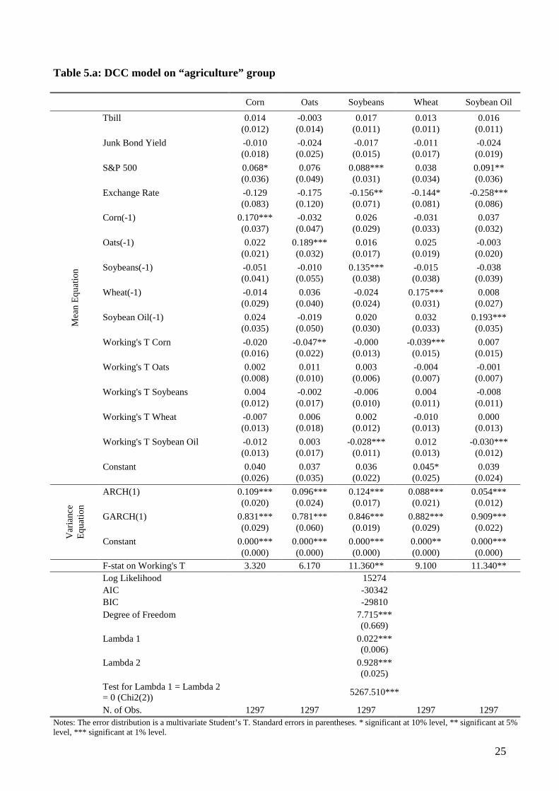
Results for the “agriculture” group of commodities are reported in Tables 5.a-5.b. Among
macroeconomic controls, only the S&P return and the exchange rate display significant coefficients,
with the expected signs. We do not observe spillovers in the mean equation: only the own lagged
return shows positive and significant coefficients. Measures of speculation are poorly significant:
exclusively the Working’s T indexes for corn and soybean oil are significant and negative.20
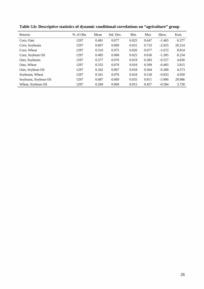
The conditional correlations implied by the DCC model reported in Table 5.b are generally high.
Contrary to the “fuels” DCC, we do not observe marked peaks in recent times. The minimum values
of the correlations are, within this group, always positive, meaning that the substitution in risk is
absent in these futures markets.
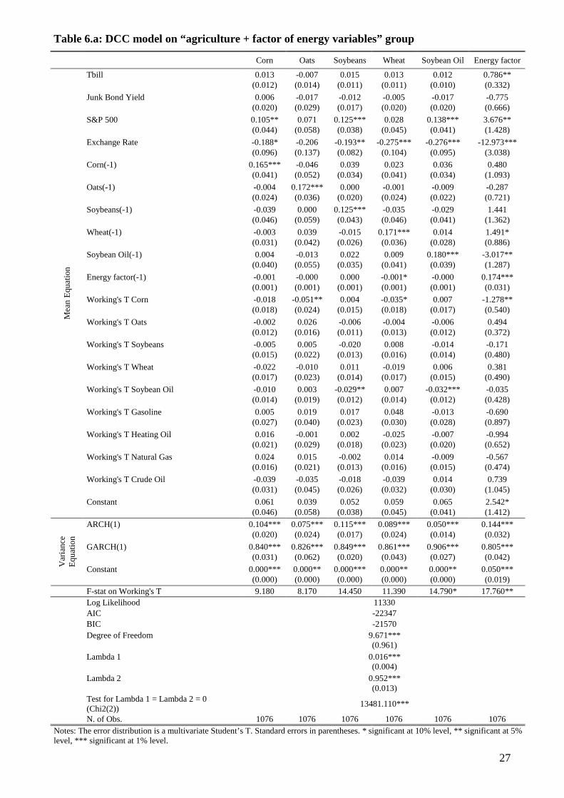
Finally, we discuss the results for the extended group, which includes agricultural commodities and
a factor summarizing the four energy variables, which has been obtained using the principal factor 18 For the full set of dynamic conditional correlation plots refer to the statistical appendix. 19 These values are on average slightly smaller than the correlations obtained in the CCC model which are reported in the statistical appendix 20 Notice that results for this group are on a longer time span relative to the “fuels” group. Results on the same interval are unchanged and are reported in the statistical appendix.
14
method to analyze the correlation matrix among the returns of the four energy commodities. Results
reported in Tables 6.a-6.b confirm previous evidence concerning the five agricultural commodities.
However, we observe no evident spillover in the mean equation among food commodities, a biofuel
and the energy factor.
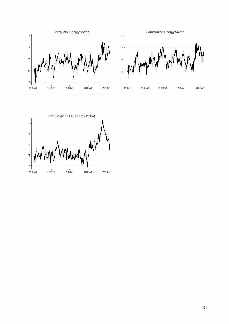
The dynamic conditional correlations, reported in Table 6.b, are generally positive. Interestingly,
the correlations between the energy factor and the other commodities are mainly low, with the
highest value being the correlation with soybean oil (0.143). Figure 1 reports the dynamic
conditional correlations, and shows that, while being on average small, the conditional correlations
with the energy factor display a peak around year 2008. The descriptive statistics reported in Table
6.b show that negative values exist only when considering correlations with the energy factor:
negative correlations indicate that high volatility values in the energy markets correspond to low
volatility levels in the markets for agricultural commodities.
5.1 Sensitivity over time
Our sample has a long time span, so it is interesting to see if spillover effects in the volatility of
commodity returns become more marked in recent years. This is shown in Table 7.a, where are
reported mean tests on dynamic conditional correlations of “fuels” group. Mean values are
statistically different at 1% level in the two samples. In particular, values after 2004 are higher and
mean values between energy commodities and soybean oil are almost doubled in the second period.
This result confirms the increasing interaction between markets, especially when biofuels are
considered. Table 7.b shows that, also for the “agriculture” group, mean values have increased after
2004, but, this time, the increase is less sharp and the relationship with biofuels is less marked.
Finally, Table 7.c confirms that, also in this last group, mean values of dynamic conditional
correlations between agricultural commodities and the energy factor are more than doubled after
2004.
We investigate if there are changes in mean equations before and after 2004 in the results of DCC
estimations.21 As regards the “fuels” group it is relevant to notice that the influence of crude oil
(with reference to its past returns and its Working’s T index) on other commodities and, in
particular, on soybean oil, appears to be significant only after 2004, suggesting that spillovers in the
mean equation happen mostly in the last period. Interestingly, we find that the conditional
correlations increase in size after 2004 and that the correlations between fuels and soybean oil
become significant and positive, confirming again spillover effects in recent times. Results for the
“agriculture” group do not show marked differences before and after 2004. Finally, looking at the
21 These results, as well as those with CCC model, are reported in the statistical appendix.
15
“agriculture” system enriched with the energy factor, we observe that the correlations between the
energy factor and the agricultural commodities and biofuel become significant only after 2004.
These last results support once again the increasing interaction between different markets and are in
line with similar results obtained adopting alternative econometric approaches (Natanelov et al.
2011, Ciaian and Kancs 2011, Du and McPhill 2012).
6. Conclusions
The recent spike in commodities prices in 2008 has lead to claims that prices are driven by
speculators. Moreover, as the rise has affected both energy and food commodities a generalized
financialization of commodities futures markets has been held responsible. Another channel for the
transmission of price shocks has been alleged to be the increasing relevance of biofules, which
interconnect energy and food markets. However, most of the evidence in support of these
hypotheses is based on descriptive statistics.
We collect data on futures prices for four energy commodities and five agricultural commodities
(including a biofuel, soybean oil) over the period 1986-2010 at weekly frequency and measure
financial speculation by means of the Working’s T (1960) index. With this sample we aim at
answering to four research questions. First, we look at the role of macroeconomic factors as
possible drivers of returns of energy and agricultural commodities. Second, we consider whether
financial speculation is significantly related to returns in futures markets. Third, we focus on the
relationship among returns across different markets both with respect to the mean and the variance.
Moreover, we investigate if and how speculation in one market affects returns in other markets.
Descriptive evidence shows that the Working’s T index has significantly increased after 2004 only
in crude oil, natural gas and wheat futures markets. Additionally, the correlations with commodities
returns are generally not significant.
The econometric exercise presents an univariate analysis where commodity returns are modelled
according to a GARCH(1,1)-AR(1) term. Working’s T index is negative or not significant: a
negative sign implies that an increase in excess speculation corresponds to a decrease in returns.
This result contrasts with the claims in the literature that speculation has affected returns in a
positive way (Eckaus 2008, Masters 2008, Soros 2008). Among macroeconomic factors, S&P500
index is positive and significant and the exchange rate is negative and generally significant,
suggesting that a depreciation of U.S. dollar increases futures prices.
To analyze spillovers between commodities and different futures markets we present results from
multivariate GARCH models. We group the commodities into two subgroups, “fuels” (gasoline,

16
heating oil, natural gas, crude oil and soybean oil) and “agriculture” (corn, oats, soybeans, wheat
and soybean oil). As in the univariate case, S&P500 index is always positive and significant and the
exchange rate is generally negative and significant.
Thus, as concerns our first research question, some macroeconomic variables seem to significantly
affect the returns in commodities futures. With respect to our second research question, estimates
suggest that speculation is generally not relevant. As for the third issue, i.e. possible spillovers
across commodities, both in the mean and variance equation, we observe that lagged returns of
crude oil and natural gas positively affect returns of the other energy commodities. Looking at
volatilities, it is interesting to note that correlations between soybean oil and the other energy
commodities and those between agricultural and energy factor present higher values around 2008,
i.e. in the peak period of prices. Negative correlations between agriculture commodities and the
energy factor suggest that high (low) volatilities in the agricultural markets correspond to low (high)
volatility in the energy market. Moreover, when we distinguish between time periods, we notice
that mean values of dynamic conditional correlations always increase after 2004 and, in fuels
markets, they even double. Finally, speculation in one market does not seem to significantly affect
returns in other markets.
References
Ai, Chunrong, Arjun Chatrath and Frank Song. 2006. “On the Comovement of Commodity
Prices” American Journal of Agricultural Economics 88 (3): 574-588.
Baffes, John. 2007. “Oil spills on other commodities” Resources Policy 32 (3): 126-134.
Baffes, John. 2010. “More on the Energy/Non-Energy Price Link” Applied Economics Letters 17:
1555-1558.
Baffes, John and Tassos Haniotis. 2010. “Placing the Recent Commodity Boom into Perspective”
in M. Ataman Aksoy and Bernard M. Hoekman, eds., Food Prices and Rural Poverty. Washington
DC: The International Bank for reconstruction and Development-The World Bank: 41-70.
Bastianin, Andrea, Matteo Manera, Marcella Nicolini and Ilaria Vignati. 2012. “Speculation,
Returns, Volume and Volatility in Commodities Futures Markets” Review of Environment, Energy
and Economics, January 20, 2012.
Brunetti, Celso, and Bahattin Büyükşahin. 2009. Is Speculation Destabilizing? U.S. Commodity
Futures Trading Commission Working Paper.
17
Büyükşahin, Bahattin and Jeffrey H. Harris. 2011. “Do Speculators Drive Crude Oil Futures
Prices?” The Energy Journal 32 (2): 167-202.
Chang, Chia-Lin, Michael McAleer and Roengchai Tansuchat. 2009. “Modeling conditional
correlations for risk diversification in crude oil markets” Journal of Energy Markets 2: 29-51.
Chang, Chia-Lin, Michael McAleer and Roengchai Tansuchat. 2011. “Crude oil hedging
strategies using dynamic multivariate GARCH” Energy Economics 33: 912-923.
Chaudhuri, Kausik. 2001. “Long-run prices of primary commodities and oil prices” Applied
Economics 33 (4): 531-538.
Chen, Yu-Chin, Kenneth S. Rogoff and Barbara Rossi. 2010. “Can exchange rate forecast
commodity prices?” Quarterly Journal of Economics 125 (3): 1145–1194.
Chevallier, Julien. 2009. “Carbon Futures and Macroeconomic Risk Factors: a View from the EU
ETS” Energy Economics 31: 614-625.
Ciaian, Pavel and d’Artis Kancs. 2011. “Food, energy and environment: Is bioenergy the missing
link?” Food Policy 36: 571-580.
Deb, Partha, Pravin K. Trivedi and Panayotis Varangis. 1996. “The Excess Co-Movement of
Commodity Prices Reconsidered” Journal of Applied Econometrics 11 (3): 275-291.
Du, Xiaodong and Lihong Lu McPhail. 2012. “Inside the Black Box: the Price Linkage and
Transmission between Energy and Agricultural Markets” The Energy Journal 33 (2): 171-194.
Du, Xiaodong, Cindy L. Yu and Dermot J. Hayes. 2011. “Speculation and volatility spillover in
the crude oil and agricultural commodity markets: A Bayesian analysis” Energy Economics 33:
497-503.
Eckaus, Richard S. 2008. “The Oil Price Really Is A Speculative Bubble” Center for Energy and
Environmental Policy Research 08-007.
Engle, Robert F. 2009. Anticipating Correlations A New Paradigm for Risk Management.
Princeton, NJ: Princeton University Press.
Frankel, Jeff A. 2008a. “Commodity Prices, Again: Are Speculators to Blame?”
http://content.ksg.harvard.edu/blog/jeff_frankels_weblog/2008/07/25/commodity-prices-again-are-
speculators-to-blame.
Frankel, Jeff A. 2008b. “The Effect of Monetary Policy on Real Commodity Prices” in John Y.
Campbell, ed., Asset Prices and Monetary Policy: 291 – 333.
18
Gilbert, Christopher L. 2010. “How to Understand High Food Prices” Journal of Agricultural
Economics 61 (2): 398-425.
Irwin, Scott H. and Dwight R. Sanders. 2012. “Testing the Masters Hypothesis in commodity
futures markets” Energy Economics 34: 256-269.
Kaufmann, Robert K. and Ben Ulman. 2009. “Oil prices, speculation, and fundamentals:
Interpreting causal relations among spot and futures prices” Energy Economics 31: 550-558.
Kaufmann, Robert K. 2011. “The role of market fundamentals and speculation in recent price
changes for crude oil” Energy Policy 39: 105-115.
Khan, Moshin S. 2009. “The 2008 Oil Price “Bubble”” Peterson Institute for International
Economics No. PB09-19.
Lanza, Alessandro, Matteo Manera and Michael McAleer. 2006. “Modeling dynamic conditional
correlations in WTI oil forward and future returns” Finance Research Letters 3 (2): 114-132.
Leybourne, Stephen J., Tim A. Lloyd and Geoffrey V. Reed. 1994. “The Excess Comovement of
Commodity Prices Revisited” World Development 22 (11): 1747-1758.
Malliaris, Anastasios G. and Jorge L. Urrutia. 1996. “Linkages Between Agricultural Commodity
Futures Contracts” Journal of Futures Markets 16 (5): 595-609.
Manera, Matteo, Michael McAleer and Margherita Grasso. 2006. “Modeling time-varying
conditional correlations in the volatility of Tapis oil spot and forward returns” Applied Financial
Economics 16 (7): 525-533.
Masters, Michael W. 2008. “Testimony of Michael W. Masters before the Committee on
Homeland Security and Governmental Affairs United States Senate”, May 2008.
http://hsgac.senate.gov/public/_files/052008Masters.pdf.
McAleer, Michael, Felix Chan and Dora Marinova. 2007. “An econometric analysis of
asymmetric volatility: theory and application to patents” Journal of Econometrics 139 (2): 259-284.
Medlock III, Kenneth B. and Amy M. Jaffe. 2009. “Who Is In the Oil Futures Market and How
Has It Changed?” James A. Baker III Institute for Public Policy, Rice University.
Mitchell, Donald. 2008. “A Note on Rising Food Prices” Policy Research Working Paper No.
4682.
Natanelov, Valeri, Mohammad J. Alam, Andrew M. McKenzie and Guido Van Huylenbroeck.
2011. “Is there co-movement of agricultural commodities futures prices and crude oil?” Energy
Policy 39: 4971-4984.

19
Pindyck, Robert S. and Julio J. Rotemberg. 1990. “The Excess Co-Movement of Commodity
Prices” The Economic Journal 100 (403): 1173-1189.
Robles, Miguel, Maximo Torero and Joachim von Braun. 2009. “When Speculation Matters”
International Food Policy Research Institute, Issue Brief 57.
Sadorsky, Perry. 2002. “Time-varying Risk Premiums in Petroleum Futures Prices” Energy
Economics 24: 539-556.
Sanders, Dwight R., Scott H. Irwin and Robert P. Merrin. 2010. “The Adequacy of Speculation in
Agricultural Futures Markets: Too Much of a Good Thing?” Applied Economic Perspectives and
Policy 32 (1): 77-94.
Smith, James L. 2009. “World Oil: Market or Mayhem?” Journal of Economic Perspectives 23
(3): 145-164.
Soros, George. 2008. “Testimony before the U.S. Senate Commerce Committee Oversight
Hearing on FTC Advanced Rulemaking on Oil Market Manipulation”, June 2008.
http://www.georgesoros.com/files/SorosFinal-Testimony.pdf.
Stoll, Hans R. and Robert E. Whaley. 2010. “Commodity Index Investing and Commodity
Futures Prices” Journal of Applied Finance 20 (1): 7-46.
Till, Hilary. 2009. “Has There Been Excessive Speculation in the US Oil Futures Markets?”
EDHEC-Risk Institute Position Paper.
Trostle, Ronald. 2008. “Global Agricultural Supply and Demand: Factors Contributing to the
Recent Increase in Food Commodity Prices”. United States Department of Agriculture, WRS-0801.
U.S. Energy Information Administration (EIA). 2008. Short Term Energy Outlook, 2008-07.
Verleger, Philip K. 2009. “The Role of Speculators in Setting the Price of Oil”, Testimony to
U.S. Commodities Futures Trading Commission.
http://www.cftc.gov/ucm/groups/public/@newsroom/documents/file/hearing080509_verleger.pdf.
Working, Holbrook. 1960. “Speculation on Hedging Markets” Food Research Institute Studies
1:185-220.
20
Tables and Figures
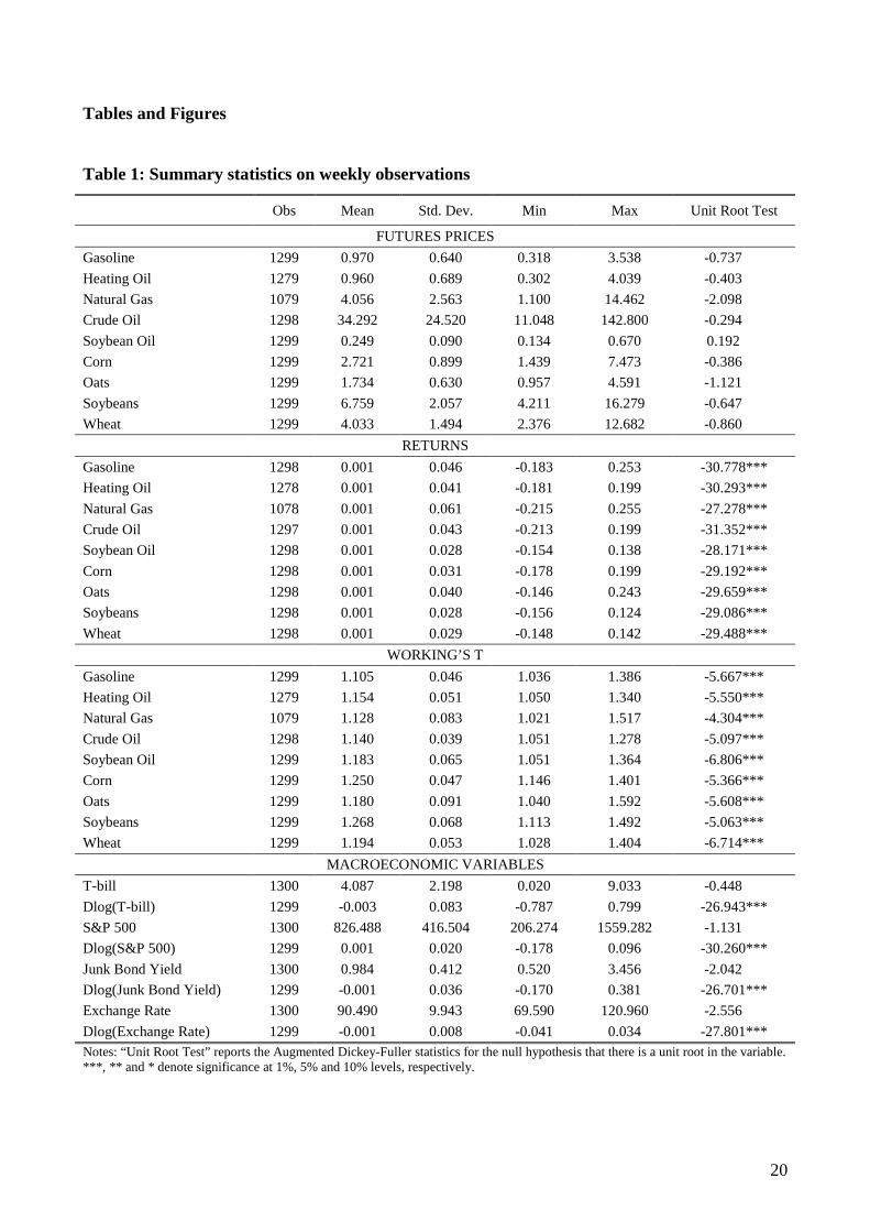
Table 1: Summary statistics on weekly observations
Obs Mean Std. Dev. Min Max Unit Root Test
FUTURES PRICES
Gasoline 1299 0.970 0.640 0.318 3.538 -0.737***
Heating Oil 1279 0.960 0.689 0.302 4.039 -0.403***
Natural Gas 1079 4.056 2.563 1.100 14.462 -2.098***
Crude Oil 1298 34.292 24.520 11.048 142.800 -0.294***
Soybean Oil 1299 0.249 0.090 0.134 0.670 0.192***
Corn 1299 2.721 0.899 1.439 7.473 -0.386***
Oats 1299 1.734 0.630 0.957 4.591 -1.121***
Soybeans 1299 6.759 2.057 4.211 16.279 -0.647***
Wheat 1299 4.033 1.494 2.376 12.682 -0.860***
RETURNS Gasoline 1298 0.001 0.046 -0.183 0.253 -30.778***
Heating Oil 1278 0.001 0.041 -0.181 0.199 -30.293***
Natural Gas 1078 0.001 0.061 -0.215 0.255 -27.278***
Crude Oil 1297 0.001 0.043 -0.213 0.199 -31.352***
Soybean Oil 1298 0.001 0.028 -0.154 0.138 -28.171***
Corn 1298 0.001 0.031 -0.178 0.199 -29.192***
Oats 1298 0.001 0.040 -0.146 0.243 -29.659***
Soybeans 1298 0.001 0.028 -0.156 0.124 -29.086***
Wheat 1298 0.001 0.029 -0.148 0.142 -29.488***
WORKING’S T Gasoline 1299 1.105 0.046 1.036 1.386 -5.667***
Heating Oil 1279 1.154 0.051 1.050 1.340 -5.550***
Natural Gas 1079 1.128 0.083 1.021 1.517 -4.304***
Crude Oil 1298 1.140 0.039 1.051 1.278 -5.097***
Soybean Oil 1299 1.183 0.065 1.051 1.364 -6.806***
Corn 1299 1.250 0.047 1.146 1.401 -5.366***
Oats 1299 1.180 0.091 1.040 1.592 -5.608***
Soybeans 1299 1.268 0.068 1.113 1.492 -5.063***
Wheat 1299 1.194 0.053 1.028 1.404 -6.714***
MACROECONOMIC VARIABLES T-bill 1300 4.087 2.198 0.020 9.033 -0.448***
Dlog(T-bill) 1299 -0.003 0.083 -0.787 0.799 -26.943***
S&P 500 1300 826.488 416.504 206.274 1559.282 -1.131***
Dlog(S&P 500) 1299 0.001 0.020 -0.178 0.096 -30.260***
Junk Bond Yield 1300 0.984 0.412 0.520 3.456 -2.042***
Dlog(Junk Bond Yield) 1299 -0.001 0.036 -0.170 0.381 -26.701***
Exchange Rate 1300 90.490 9.943 69.590 120.960 -2.556***
Dlog(Exchange Rate) 1299 -0.001 0.008 -0.041 0.034 -27.801*** Notes: “Unit Root Test” reports the Augmented Dickey-Fuller statistics for the null hypothesis that there is a unit root in the variable. ***, ** and * denote significance at 1%, 5% and 10% levels, respectively.
21
Table 2: Summary statistics on Working’s T index
Obs Mean Std. Dev. Min Max Commodity
1986-2003 2004-2010 1986-2003 2004-2010 t-stat 1986-2003 2004-2010 1986-2003 2004-2010 1986-2003 2004-2010
Gasoline 935 364 1.116 1.076 15.070*** 0.049 0.020 1.036 1.042 1.386 1.155
Heating Oil 915 364 1.161 1.136 8.189*** 0.053 0.039 1.050 1.072 1.340 1.259
Natural Gas 715 364 1.084 1.213 -35.554*** 0.044 0.075 1.021 1.097 1.517 1.478 ENERGY
Crude Oil 935 363 1.135 1.150 -6.004*** 0.043 0.027 1.051 1.090 1.278 1.232
Soybean Oil 935 364 1.203 1.133 19.992*** 0.058 0.053 1.051 1.054 1.364 1.267
Corn 935 364 1.262 1.219 16.148*** 0.043 0.043 1.172 1.146 1.401 1.319
Oats 935 364 1.193 1.146 8.690*** 0.093 0.076 1.053 1.040 1.592 1.435
Soybeans 935 364 1.288 1.217 19.124*** 0.065 0.047 1.113 1.113 1.492 1.327
AGRICULTURE
Wheat 935 364 1.181 1.225 -14.383*** 0.044 0.061 1.028 1.102 1.404 1.382
Notes: t-stat is the mean test; * significant at 10% level, ** significant at 5% level, *** significant at 1% level.
22
Table 3: Estimates of the univariate specification
Gasoline Heating Oil Natural Gas Crude Oil Soybean Oil Corn Oats Soybeans Wheat
Tbill 0.039** 0.028** 0.016 0.022 0.013 0.018* -0.001 0.010 0.011
(0.015) (0.012) (0.017) (0.014) (0.009) (0.011) (0.012) (0.010) (0.011)
Junk Bond Yield -0.050 -0.023 0.056 -0.033 -0.012 -0.011 -0.017 -0.021 -0.003
(0.032) (0.027) (0.050) (0.027) (0.019) (0.021) (0.028) (0.018) (0.019)
S&P 500 0.068 0.106** 0.152* 0.134*** 0.103*** 0.073** 0.065 0.094*** 0.038
(0.054) (0.050) (0.082) (0.050) (0.035) (0.036) (0.049) (0.033) (0.036)
Exchange Rate -0.347*** -0.564*** -0.135 -0.385*** -0.267*** -0.159* -0.268** -0.197*** -0.118
(0.134) (0.115) (0.189) (0.121) (0.089) (0.087) (0.119) (0.073) (0.084)
Working’s T -0.083*** -0.080*** -0.057** 0.008 -0.052*** -0.027 -0.002 -0.026** -0.020
(0.029) (0.021) (0.025) (0.027) (0.012) (0.018) (0.012) (0.010) (0.016)
AR(1) 0.179*** 0.161*** 0.199*** 0.156*** 0.208*** 0.201*** 0.174*** 0.201*** 0.209***
(0.028) (0.030) (0.033) (0.029) (0.028) (0.028) (0.028) (0.030) (0.028)
Constant -0.093*** 0.094*** 0.066** -0.008 0.063*** 0.035 0.002 0.034** 0.024
Me
an E
qu
atio
n
(0.032) (0.024) (0.028) (0.031) (0.014) (0.022) (0.014) (0.013) (0.019)
ARCH(1) 0.114*** 0.166*** 0.153*** 0.130*** 0.072*** 0.151*** 0.115*** 0.173*** 0.087***
(0.025) (0.029) (0.037) (0.027) (0.019) (0.030) (0.032) (0.029) (0.018)
GARCH(1) 0.828*** 0.741*** 0.765*** 0.825*** 0.875*** 0.793*** 0.766*** 0.794*** 0.892***
(0.037) (0.046) (0.053) (0.034) (0.035) (0.038) (0.063) (0.030) (0.022)
Constant 0.000*** 0.000*** 0.000*** 0.000*** 0.000** 0.000*** 0.000*** 0.000*** 0.000**
Va
ria
nce
E
qu
atio
n
(0.000) (0.000) (0.000) (0.000) (0.000) (0.000) (0.000) (0.000) (0.000)
LM test for ARCH 68.025*** 167.973*** 8.678*** 56.957*** 29.917*** 23.701*** 88.460*** 30.089*** 32.350*** Ljung-Box Q test (lag 1) 2.072 0.042 0.568 0.543 0.557 0.022 0.529 0.038 0.404 Log Likelihood 2286 2405 1560 2402 2922 2816 2442 2997 2888 AIC -4550 -4788 -3099 -4782 -5821 -5611 -4862 -5971 -5754 BIC -4493 -4732 -3044 -4725 -5764 -5554 -4805 -5914 -5698 N. of Obs. 1298 1278 1078 1297 1298 1298 1298 1298 1298
Notes: The error distribution is a Student’s T. Standard errors in parentheses. * significant at 10% level, ** significant at 5% level, *** significant at 1% level.
23
Table 4.a: DCC model on “fuels” group Gasoline Heating Oil Natural Gas Crude Oil Soybean Oil
Tbill 0.038** 0.020 0.005 0.021 0.007 (0.016) (0.013) (0.018) (0.015) (0.011)
Junk Bond Yield -0.037 -0.019 0.035 -0.046 -0.001 (0.033) (0.028) (0.046) (0.030) (0.020)
S&P 500 0.134* 0.150** 0.196** 0.141** 0.148*** (0.069) (0.060) (0.089) (0.064) (0.042)
Exchange Rate -0.411*** -0.578*** -0.147 -0.555*** -0.337*** (0.150) (0.129) (0.210) (0.133) (0.098)
Gasoline(-1) 0.063 -0.042 -0.091 -0.022 0.034 (0.045) (0.037) (0.056) (0.038) (0.025)
Heating Oil(-1) -0.116** -0.027 -0.019 -0.064 -0.014 (0.055) (0.051) (0.070) (0.052) (0.031)
Natural Gas(-1) 0.042** 0.064*** 0.193*** 0.060*** -0.036*** (0.020) (0.018) (0.034) (0.018) (0.012)
Crude Oil(-1) 0.183*** 0.206*** 0.114* 0.192*** -0.021 (0.057) (0.050) (0.067) (0.054) (0.031)
Soybean Oil(-1) -0.009 -0.048 -0.063 -0.053 0.186*** (0.045) (0.038) (0.061) (0.039) (0.032)
Working's T Gasoline -0.097** 0.015 0.090 -0.055 0.006 (0.045) (0.038) (0.065) (0.038) (0.029)
Working's T Heating Oil 0.000 -0.062** -0.058 -0.031 -0.029 (0.031) (0.027) (0.045) (0.027) (0.020)
Working's T Natural Gas 0.007 0.002 -0.051* -0.001 -0.002 (0.021) (0.018) (0.027) (0.019) (0.014)
Working's T Crude Oil -0.008 0.023 0.031 0.029 0.022 (0.051) (0.044) (0.063) (0.045) (0.030)
Working's T Soybean Oil -0.016 -0.014 -0.062** -0.010 -0.042*** (0.019) (0.016) (0.028) (0.017) (0.011)
Constant 0.128** 0.045 0.064 0.078 0.054*
Mea
n E
qu
atio
n
(0.056) (0.048) (0.076) (0.050) (0.033)
ARCH(1) 0.091*** 0.093*** 0.145*** 0.105*** 0.154*** (0.021) (0.017) (0.032) (0.016) (0.047)
GARCH(1) 0.828*** 0.850*** 0.760*** 0.844*** 0.696*** (0.042) (0.028) (0.044) (0.020) (0.108)
Constant 0.000*** 0.000*** 0.000*** 0.000*** 0.000**
Var
ian
ce
Eq
uat
ion
(0.000) (0.000) (0.000) (0.000) (0.000)
F-stat on Working's T 13.770** 8.790 8.630 10.310* 18.910***
Log Likelihood 11136 AIC -22067 BIC -21554 Degree of Freedom 9.724*** (1.065)
Lambda 1 0.050*** (0.009)
Lambda 2 0.816*** (0.038)
Test for Lambda 1 = Lambda 2 = 0 (Chi2(2))
1400.520***
N. of Obs. 1076 1076 1076 1076 1076 Notes: The error distribution is a multivariate Student’s T. Standard errors in parentheses. * significant at 10% level, ** significant at 5% level, *** significant at 1% level.
24
Table 4.b: Descriptive statistics of dynamic conditional correlations on “fuels” group
Returns N. of Obs. Mean Std. Dev. Min Max Skew. Kurt.
Gasoline, Heating Oil 1076 0.706 0.064 0.100 0.852 -2.256 16.889
Gasoline, Natural Gas 1076 0.219 0.084 -0.199 0.568 -0.341 4.721
Gasoline, Crude Oil 1076 0.723 0.059 0.102 0.855 -3.086 25.343
Gasoline, Soybean Oil 1076 0.130 0.089 -0.112 0.490 0.533 4.279
Heating Oil, Natural Gas 1076 0.330 0.075 0.047 0.574 -0.267 3.317
Heating Oil, Crude Oil 1076 0.773 0.059 0.108 0.875 -4.115 35.206
Heating Oil, Soybean Oil 1076 0.164 0.097 -0.136 0.466 0.296 3.523
Natural Gas, Crude Oil 1076 0.219 0.082 -0.206 0.430 -0.832 5.120
Natural Gas, Soybean Oil 1076 0.129 0.076 -0.090 0.419 0.287 3.203
Crude Oil, Soybean Oil 1076 0.126 0.094 -0.146 0.519 0.478 4.175
25
Table 5.a: DCC model on “agriculture” group
Corn Oats Soybeans Wheat Soybean Oil
Tbill 0.014 -0.003 0.017 0.013 0.016 (0.012) (0.014) (0.011) (0.011) (0.011)
Junk Bond Yield -0.010 -0.024 -0.017 -0.011 -0.024 (0.018) (0.025) (0.015) (0.017) (0.019)
S&P 500 0.068* 0.076 0.088*** 0.038 0.091** (0.036) (0.049) (0.031) (0.034) (0.036)
Exchange Rate -0.129 -0.175 -0.156** -0.144* -0.258*** (0.083) (0.120) (0.071) (0.081) (0.086)
Corn(-1) 0.170*** -0.032 0.026 -0.031 0.037 (0.037) (0.047) (0.029) (0.033) (0.032)
Oats(-1) 0.022 0.189*** 0.016 0.025 -0.003 (0.021) (0.032) (0.017) (0.019) (0.020)
Soybeans(-1) -0.051 -0.010 0.135*** -0.015 -0.038 (0.041) (0.055) (0.038) (0.038) (0.039)
Wheat(-1) -0.014 0.036 -0.024 0.175*** 0.008 (0.029) (0.040) (0.024) (0.031) (0.027)
Soybean Oil(-1) 0.024 -0.019 0.020 0.032 0.193*** (0.035) (0.050) (0.030) (0.033) (0.035)
Working's T Corn -0.020 -0.047** -0.000 -0.039*** 0.007 (0.016) (0.022) (0.013) (0.015) (0.015)
Working's T Oats 0.002 0.011 0.003 -0.004 -0.001 (0.008) (0.010) (0.006) (0.007) (0.007)
Working's T Soybeans 0.004 -0.002 -0.006 0.004 -0.008 (0.012) (0.017) (0.010) (0.011) (0.011)
Working's T Wheat -0.007 0.006 0.002 -0.010 0.000 (0.013) (0.018) (0.012) (0.013) (0.013)
Working's T Soybean Oil -0.012 0.003 -0.028*** 0.012 -0.030*** (0.013) (0.017) (0.011) (0.013) (0.012)
Constant 0.040 0.037 0.036 0.045* 0.039
Mea
n E
qu
atio
n
(0.026) (0.035) (0.022) (0.025) (0.024)
ARCH(1) 0.109*** 0.096*** 0.124*** 0.088*** 0.054*** (0.020) (0.024) (0.017) (0.021) (0.012)
GARCH(1) 0.831*** 0.781*** 0.846*** 0.882*** 0.909*** (0.029) (0.060) (0.019) (0.029) (0.022)
Constant 0.000*** 0.000*** 0.000*** 0.000** 0.000***
Var
ian
ce
Eq
uat
ion
(0.000) (0.000) (0.000) (0.000) (0.000)
F-stat on Working's T 3.320 6.170 11.360** 9.100 11.340**
Log Likelihood 15274 AIC -30342 BIC -29810 Degree of Freedom 7.715*** (0.669)
Lambda 1 0.022*** (0.006)
Lambda 2 0.928*** (0.025)
Test for Lambda 1 = Lambda 2 = 0 (Chi2(2))
5267.510***
N. of Obs. 1297 1297 1297 1297 1297 Notes: The error distribution is a multivariate Student’s T. Standard errors in parentheses. * significant at 10% level, ** significant at 5% level, *** significant at 1% level.
26
Table 5.b: Descriptive statistics of dynamic conditional correlations on “agriculture” group
Returns N. of Obs. Mean Std. Dev. Min Max Skew. Kurt.
Corn, Oats 1297 0.481 0.077 0.025 0.647 -1.465 6.377
Corn, Soybeans 1297 0.607 0.069 0.031 0.733 -2.925 20.214
Corn, Wheat 1297 0.510 0.075 0.026 0.677 -1.672 8.814
Corn, Soybean Oil 1297 0.485 0.068 0.025 0.636 -1.305 8.234
Oats, Soybeans 1297 0.377 0.070 0.019 0.583 -0.527 4.830
Oats, Wheat 1297 0.355 0.070 0.018 0.599 -0.405 3.815
Oats, Soybean Oil 1297 0.342 0.067 0.018 0.564 -0.368 4.573
Soybeans, Wheat 1297 0.341 0.076 0.018 0.518 -0.833 4.050
Soybeans, Soybean Oil 1297 0.687 0.069 0.035 0.811 -3.906 29.986
Wheat, Soybean Oil 1297 0.284 0.069 0.015 0.457 -0.584 3.730
27
Table 6.a: DCC model on “agriculture + factor of energy variables” group
Corn Oats Soybeans Wheat Soybean Oil Energy factor
Tbill 0.013 -0.007 0.015 0.013 0.012 0.786** (0.012) (0.014) (0.011) (0.011) (0.010) (0.332)
Junk Bond Yield 0.006 -0.017 -0.012 -0.005 -0.017 -0.775 (0.020) (0.029) (0.017) (0.020) (0.020) (0.666)
S&P 500 0.105** 0.071 0.125*** 0.028 0.138*** 3.676** (0.044) (0.058) (0.038) (0.045) (0.041) (1.428)
Exchange Rate -0.188* -0.206 -0.193** -0.275*** -0.276*** -12.973*** (0.096) (0.137) (0.082) (0.104) (0.095) (3.038)
Corn(-1) 0.165*** -0.046 0.039 0.023 0.036 0.480 (0.041) (0.052) (0.034) (0.041) (0.034) (1.093)
Oats(-1) -0.004 0.172*** 0.000 -0.001 -0.009 -0.287 (0.024) (0.036) (0.020) (0.024) (0.022) (0.721)
Soybeans(-1) -0.039 0.000 0.125*** -0.035 -0.029 1.441 (0.046) (0.059) (0.043) (0.046) (0.041) (1.362)
Wheat(-1) -0.003 0.039 -0.015 0.171*** 0.014 1.491* (0.031) (0.042) (0.026) (0.036) (0.028) (0.886)
Soybean Oil(-1) 0.004 -0.013 0.022 0.009 0.180*** -3.017** (0.040) (0.055) (0.035) (0.041) (0.039) (1.287)
Energy factor(-1) -0.001 -0.000 0.000 -0.001* -0.000 0.174*** (0.001) (0.001) (0.001) (0.001) (0.001) (0.031)
Working's T Corn -0.018 -0.051** 0.004 -0.035* 0.007 -1.278** (0.018) (0.024) (0.015) (0.018) (0.017) (0.540)
Working's T Oats -0.002 0.026 -0.006 -0.004 -0.006 0.494 (0.012) (0.016) (0.011) (0.013) (0.012) (0.372)
Working's T Soybeans -0.005 0.005 -0.020 0.008 -0.014 -0.171 (0.015) (0.022) (0.013) (0.016) (0.014) (0.480)
Working's T Wheat -0.022 -0.010 0.011 -0.019 0.006 0.381 (0.017) (0.023) (0.014) (0.017) (0.015) (0.490)
Working's T Soybean Oil -0.010 0.003 -0.029** 0.007 -0.032*** -0.035 (0.014) (0.019) (0.012) (0.014) (0.012) (0.428)
Working's T Gasoline 0.005 0.019 0.017 0.048 -0.013 -0.690 (0.027) (0.040) (0.023) (0.030) (0.028) (0.897)
Working's T Heating Oil 0.016 -0.001 0.002 -0.025 -0.007 -0.994 (0.021) (0.029) (0.018) (0.023) (0.020) (0.652)
Working's T Natural Gas 0.024 0.015 -0.002 0.014 -0.009 -0.567 (0.016) (0.021) (0.013) (0.016) (0.015) (0.474)
Working's T Crude Oil -0.039 -0.035 -0.018 -0.039 0.014 0.739 (0.031) (0.045) (0.026) (0.032) (0.030) (1.045)
Constant 0.061 0.039 0.052 0.059 0.065 2.542*
Mea
n E
quat
ion
(0.046) (0.058) (0.038) (0.045) (0.041) (1.412)
ARCH(1) 0.104*** 0.075*** 0.115*** 0.089*** 0.050*** 0.144*** (0.020) (0.024) (0.017) (0.024) (0.014) (0.032)
GARCH(1) 0.840*** 0.826*** 0.849*** 0.861*** 0.906*** 0.805*** (0.031) (0.062) (0.020) (0.043) (0.027) (0.042)
Constant 0.000*** 0.000** 0.000*** 0.000** 0.000** 0.050***
Var
ian
ce
Eq
uat
ion
(0.000) (0.000) (0.000) (0.000) (0.000) (0.019)
F-stat on Working's T 9.180 8.170 14.450 11.390 14.790* 17.760** Log Likelihood 11330 AIC -22347 BIC -21570 Degree of Freedom 9.671*** (0.961) Lambda 1 0.016*** (0.004) Lambda 2 0.952*** (0.013)
Test for Lambda 1 = Lambda 2 = 0 (Chi2(2))
13481.110***
N. of Obs. 1076 1076 1076 1076 1076 1076 Notes: The error distribution is a multivariate Student’s T. Standard errors in parentheses. * significant at 10% level, ** significant at 5% level, *** significant at 1% level.
28
Table 6.b: Descriptive statistics for dynamic conditional correlations on “agriculture + factor of energy variables” group
Returns N. of Obs. Mean Std. Dev. Min Max Skew. Kurt.
Corn, Oats 1076 0.488 0.073 0.016 0.605 -2.218 10.706
Corn, Soybeans 1076 0.592 0.075 0.019 0.703 -3.233 19.297
Corn, Wheat 1076 0.514 0.080 0.017 0.665 -2.102 11.044
Corn, Soybean Oil 1076 0.464 0.068 0.015 0.592 -1.909 10.613
Corn, Energy factor 1076 0.060 0.062 -0.057 0.306 1.063 4.500
Oats, Soybeans 1076 0.345 0.060 0.011 0.539 -0.676 5.206
Oats, Wheat 1076 0.357 0.067 0.012 0.496 -0.990 5.836
Oats, Soybean Oil 1076 0.318 0.055 0.010 0.522 -0.454 5.572
Oats, Energy factor 1076 0.072 0.060 -0.111 0.248 0.188 3.007
Soybeans, Wheat 1076 0.329 0.070 0.011 0.477 -0.916 4.410
Soybeans, Soybean Oil 1076 0.680 0.081 0.022 0.798 -3.657 23.293
Soybeans, Energy factor 1076 0.119 0.068 -0.026 0.380 0.977 4.372
Wheat, Soybean Oil 1076 0.284 0.064 0.010 0.447 -0.555 4.163
Wheat, Energy factor 1076 0.091 0.052 -0.056 0.239 0.298 2.506
Soybean Oil, Energy factor 1076 0.143 0.083 -0.024 0.435 1.138 4.114
Table 7.a: Mean tests on dynamic conditional correlations of “fuels” group
Obs. Mean Returns
Before 2004 After 2004 Before 2004 After 2004 t-stat
Gasoline, Heating Oil 713 363 0.692 0.733 -10.340***
Gasoline, Natural Gas 713 363 0.203 0.250 -8.946***
Gasoline, Crude Oil 713 363 0.717 0.733 -4.290***
Gasoline, Soybean Oil 713 363 0.104 0.182 -15.046***
Heating Oil, Natural Gas 713 363 0.320 0.350 -6.355***
Heating Oil, Crude Oil 713 363 0.767 0.786 -5.262***
Heating Oil, Soybean Oil 713 363 0.134 0.223 -15.924***
Natural Gas, Crude Oil 713 363 0.211 0.236 -4.678***
Natural Gas, Soybean Oil 713 363 0.115 0.157 -8.784***
Crude Oil, Soybean Oil 713 363 0.097 0.183 -15.981***
Notes: * significant at 10% level, ** significant at 5% level, *** significant at 1% level.
29
Table 7.b: Mean tests on dynamic conditional correlations of “agriculture” group
Obs. Mean Returns
Before 2004 After 2004 Before 2004 After 2004 t-stat
Corn, Oats 933 364 0.476 0.493 -3.646***
Corn, Soybeans 933 364 0.609 0.604 0.982***
Corn, Wheat 933 364 0.504 0.526 -4.660***
Corn, Soybean Oil 933 364 0.481 0.495 -3.381***
Oats, Soybeans 933 364 0.377 0.378 -0.122***
Oats, Wheat 933 364 0.347 0.377 -7.029***
Oats, Soybean Oil 933 364 0.334 0.362 -7.037***
Soybeans, Wheat 933 364 0.340 0.343 -0.539***
Soybeans, Soybean Oil 933 364 0.678 0.711 -7.761***
Wheat, Soybean Oil 933 364 0.277 0.302 -5.863***
Notes: * significant at 10% level, ** significant at 5% level, *** significant at 1% level.
Table 7.c: Mean tests on dynamic conditional correlations of “agriculture + factor of energy variables” group
Obs. Mean Returns
Before 2004 After 2004 Before 2004 After 2004 t-stat
Corn, Oats 713 363 0.482 0.499 -3.748***
Corn, Soybeans 713 363 0.591 0.594 -0.568***
Corn, Wheat 713 363 0.506 0.530 -4.739***
Corn, Soybean Oil 713 363 0.455 0.480 -5.716***
Corn, Energy factor 713 363 0.043 0.092 -13.260***
Oats, Soybeans 713 363 0.341 0.352 -3.099***
Oats, Wheat 713 363 0.344 0.382 -9.207***
Oats, Soybean Oil 713 363 0.305 0.343 -11.055***
Oats, Energy factor 713 363 0.059 0.096 -9.869***
Soybeans, Wheat 713 363 0.326 0.335 -1.868***
Soybeans, Soybean Oil 713 363 0.667 0.708 -8.377***
Soybeans, Energy factor 713 363 0.093 0.170 -20.795***
Wheat, Soybean Oil 713 363 0.274 0.304 -7.442***
Wheat, Energy factor 713 363 0.082 0.110 -8.477***
Soybean Oil, Energy factor 713 363 0.104 0.218 -27.458***
Notes: * significant at 10% level, ** significant at 5% level, *** significant at 1% level.
30
-.2
0.2
.4.6
1990w1 1995w1 2000w1 2005w1 2010w1
Corr(Gasoline, Soybean Oil)
-.2
0.2
.4.6
1990w1 1995w1 2000w1 2005w1 2010w1
Corr(Crude Oil, Soybean Oil)
0.1
.2.3
.4
1990w1 1995w1 2000w1 2005w1 2010w1
Corr(Soybeans, Energy factor)
Figure 1: Selected dynamic conditional correlations graphs
-.2
0.2
.4.6
1990w1 1995w1 2000w1 2005w1 2010w1
Corr(Heating Oil, Soybean Oil)
-.1
0.1
.2.3
.4
1990w1 1995w1 2000w1 2005w1 2010w1
Corr(Natural Gas, Soybean Oil)
-.1
0.1
.2.3
1990w1 1995w1 2000w1 2005w1 2010w1
Corr(Corn, Energy factor)
31
-.1
0.1
.2.3
1990w1 1995w1 2000w1 2005w1 2010w1
Corr(Wheat, Energy factor)-.
10
.1.2
.3
1990w1 1995w1 2000w1 2005w1 2010w1
Corr(Oats, Energy factor)
0.1
.2.3
.4
1990w1 1995w1 2000w1 2005w1 2010w1
Corr(Soybean Oil, Energy factor)