financial stability report - federal reserve · promoting financial stability is a key element in...

B o a r d o f G o v e r n o r s o f t h e F e d e r a l R e s e rv e S y s t e m

Financial Stability Report

November 2019

This and other Federal Reserve Board reports and publications are available online at www.federalreserve.gov/publications/default.htm.

To order copies of Federal Reserve Board publications offered in print, see the Board’s Publication Order Form

(www.federalreserve.gov/pubs/orderform.pdf)

or contact: Publications Fulfillment

Mail Stop N-127 Board of Governors of the Federal Reserve System

Washington, DC 20551(ph) 202-452-3245(fax) 202-728-5886

(email) [email protected]

Errata

The Federal Reserve revised this report on November 19, 2019, to reflect a corrected source note. The revision is listed below.

On p. 45, under the “Potential Shocks Cited in Market Outreach,” chart, the source note has been revised from “Source: Staff calculations based on data from the interdealer broker community; Bloomberg Finance LP.” to “Source: FRBNY phone survey of market and official-sector contacts from mid-August to end-September.”

https://www.federalreserve.gov/publications/default.htm

https://www.federalreserve.gov/pubs/orderform.pdf

mailto:Publications-BOG%40frb.gov?subject=info%20request

iii

Contents

Purpose . . . . . . . . . . . . . . . . . . . . . . . . . . . . . . . . . . . . . . . . . . . . . . . . . . . . . . . 1

Framework. . . . . . . . . . . . . . . . . . . . . . . . . . . . . . . . . . . . . . . . . . . . . . . . . . . . . 3

Overview . . . . . . . . . . . . . . . . . . . . . . . . . . . . . . . . . . . . . . . . . . . . . . . . . . . . . . 7

1. Asset Valuations . . . . . . . . . . . . . . . . . . . . . . . . . . . . . . . . . . . . . . . . . . . . . . 9

2. Borrowing by Businesses and Households. . . . . . . . . . . . . . . . . . . . . . . . . 19

3. Leverage in the Financial Sector . . . . . . . . . . . . . . . . . . . . . . . . . . . . . . . . 27

4. Funding Risk . . . . . . . . . . . . . . . . . . . . . . . . . . . . . . . . . . . . . . . . . . . . . . . 35

Near-Term Risks to the Financial System . . . . . . . . . . . . . . . . . . . . . . . . . . . 43

Figure Notes . . . . . . . . . . . . . . . . . . . . . . . . . . . . . . . . . . . . . . . . . . . . . . . . . . 47

Note: This report generally reflects information that was available as of November 7, 2019.

What Has Been Happening to the Liquidity of U.S. Treasury and Equity Futures Markets? . . . . . . . . . . . . . . . . . . . . . . . . . . . . . . . . . . . . . . 14

The Recent Decline in Interest Rates and Implications for Financial Stability . . . . . . . . . . . . . . . . . . . . . . . . . . . . . . . . . . . . . . . . . . . . 28

Global Stablecoins and Financial Stability . . . . . . . . . . . . . . . . . . . . . . . . . . . 40

Salient Shocks to Financial Stability Cited in Market Outreach . . . . . . . . . . 44

Boxes

1

PurposeThis report presents the Federal Reserve Board’s current assessment of the resilience of the U.S. financial system. By publishing this report, the Board intends to promote public under-standing and increase transparency and accountability for the Federal Reserve’s views on this topic.

Promoting financial stability is a key element in meeting the Federal Reserve’s dual mandate for monetary policy regarding full employment and stable prices. As we saw in the 2007–09 financial crisis, in an unstable financial system, adverse events are more likely to result in severe financial stress and disrupt the flow of credit, leading to high unemployment and great financial hardship. Monitoring and assessing financial stability also support the Fed-eral Reserve’s regulatory and supervisory activities, which promote the safety and soundness of our nation’s banks and other important financial institutions. Information gathered while monitoring the stability of the financial system helps the Federal Reserve develop its view of the salient risks to be included in the scenarios of the stress tests and its setting of the coun-tercyclical capital buffer (CCyB).1

The Board’s Financial Stability Report is similar to those published by other central banks and complements the annual report of the Financial Stability Oversight Council (FSOC), which is chaired by the Secretary of the Treasury and includes the Federal Reserve Board Chair and other financial regulators.

1 More information on the Federal Reserve’s supervisory and regulatory activities is available on the Board’s website; see the Supervision and Regulation Report (https://www.federalreserve.gov/supervisionreg/supervision-and-regulation-report.htm) as well as the webpages for Supervision and Regulation (https://www.federalreserve.gov/supervisionreg.htm) and Payment Systems (https://www.federalreserve.gov/paymentsystems.htm). Moreover, additional details about the conduct of monetary policy are also on the Board’s website; see the Monetary Policy Report (https://www.federalreserve.gov/monetarypolicy/mpr_default.htm) and the webpage for Monetary Policy (https://www.federalreserve.gov/monetarypolicy.htm).

https://www.federalreserve.gov/supervisionreg/supervision-and-regulation-report.htm

https://www.federalreserve.gov/supervisionreg.htm

https://www.federalreserve.gov/paymentsystems.htm

https://www.federalreserve.gov/monetarypolicy/mpr_default.htm

https://www.federalreserve.gov/monetarypolicy/mpr_default.htm

https://www.federalreserve.gov/monetarypolicy.htm

3

FrameworkA stable financial system, when hit by adverse events, or “shocks,” continues to meet the demands of households and businesses for financial services, such as credit provision and payment services. In contrast, in an unstable system, these same shocks are likely to have much larger effects, disrupting the flow of credit and leading to declines in employment and economic activity.

Consistent with this view of financial stability, the Federal Reserve Board’s monitoring framework distinguishes between shocks to and vulnerabilities of the financial system. Shocks, such as sudden changes to financial or economic conditions, are typically surprises and are inherently difficult to predict. Vulnerabilities tend to build up over time and are the aspects of the financial system that are most expected to cause widespread problems in times of stress. As a result, the framework focuses primarily on monitoring vulnerabilities and emphasizes four broad categories based on research.2

1. Elevated valuation pressures are signaled by asset prices that are high relative to eco-nomic fundamentals or historical norms and are often driven by an increased willingness of investors to take on risk. As such, elevated valuation pressures imply a greater possibil-ity of outsized drops in asset prices.

2. Excessive borrowing by businesses and households leaves them vulnerable to distress if their incomes decline or the assets they own fall in value. In the event of such shocks, businesses and households with high debt burdens may need to cut back spending sharply, affecting the overall level of economic activity. Moreover, when businesses and households cannot make payments on their loans, financial institutions and investors incur losses.

3. Excessive leverage within the financial sector increases the risk that financial institu-tions will not have the ability to absorb even modest losses when hit by adverse shocks. In those situations, institutions will be forced to cut back lending, sell their assets, or, in extreme cases, shut down. Such responses can substantially impair credit access for house-holds and businesses.

4. Funding risks expose the financial system to the possibility that investors will “run” by withdrawing their funds from a particular institution or sector. Many financial institu-tions raise funds from the public with a commitment to return their investors’ money on short notice, but those institutions then invest much of the funds in illiquid assets that are hard to sell quickly or in assets that have a long maturity. This liquidity and maturity

2 For a review of the research literature in this area and further discussion, see Tobias Adrian, Daniel Covitz, and Nellie Liang (2015), “Financial Stability Monitoring,” Annual Review of Financial Economics, vol. 7 (December), pp. 357–95.

4 Framework

transformation can create an incentive for investors to withdraw funds quickly in adverse situations. Facing a run, financial institutions may need to sell assets quickly at “fire sale” prices, thereby incurring substantial losses and potentially even becoming insolvent. Histo rians and economists often refer to widespread investor runs as “financial panics.”

These vulnerabilities often interact with each other. For example, elevated valuation pres-sures tend to be associated with excessive borrowing by businesses and households because both borrowers and lenders are more willing to accept higher degrees of risk and leverage when asset prices are appreciating rapidly. The associated debt and leverage, in turn, make the risk of outsized declines in asset prices more likely and more damaging. Similarly, the risk of a run on a financial institution and the consequent fire sales of assets are greatly amplified when significant leverage is involved.

It is important to note that liquidity and maturity transformation and lending to households, businesses, and financial firms are key aspects of how the financial system supports the economy. For example, banks provide safe, liquid assets to depositors and long-term loans to households and businesses; businesses rely on loans or bonds to fund investment projects; and households benefit from a well-functioning mortgage market when buying a home.

The Federal Reserve’s monitoring framework also tracks domestic and international devel-opments to identify near-term risks—that is, plausible adverse developments or shocks that could stress the U.S. financial system. The analysis of these risks focuses on assessing how such potential shocks may play out through the U.S. financial system, given our current assessment of the four areas of vulnerabilities.

While this framework provides a systematic way to assess financial stability, some potential risks do not fit neatly into it because they are novel or difficult to quantify. For example, cybersecurity and developments in crypto-assets are the subject of monitoring and policy efforts that may be addressed in future discussions of risks.3 In addition, some vulnerabili-ties are difficult to measure with currently available data, and the set of vulnerabilities may evolve over time. Given these limitations, we continually rely on ongoing research by the Federal Reserve staff, academics, and other experts to improve our measurement of existing vulnerabilities and to keep pace with changes in the financial system that could create new forms of vulnerabilities or add to existing ones.

Federal Reserve actions to promote the resilience of the financial system

The assessment of financial vulnerabilities informs Federal Reserve actions to promote the resilience of the financial system. The Federal Reserve works with other domestic agencies

3 This report does not currently provide a standard set of metrics for determining the cyber resilience of systems that are deemed to be critical to maintaining U.S. financial stability. Nonetheless, the Federal Reserve is using the available informa-tion and working with the relevant domestic agencies to develop resilience expectations and measures.

FINaNCIaL STaBILITY rePorT: NoVemBer 2019 5

directly and through the FSOC to monitor risks to financial stability and to undertake super-visory and regulatory efforts to mitigate the risks and consequences of financial instability.

Actions taken by the Federal Reserve to promote the resilience of the financial system include its supervision and regulation of financial institutions—in particular, large bank holding companies (BHCs), the U.S. operations of certain foreign banking organizations, and financial market utilities. Specifically, in the post-crisis period, for the largest, most sys-temically important BHCs, these actions have included requirements for more and higher- quality capital, an innovative stress-testing regime, new liquidity regulation, and improve-ments in the resolvability of such BHCs.

In addition, the Federal Reserve’s assessment of financial vulnerabilities informs the design of stress-test scenarios and decisions regarding the CCyB. The stress scenarios incorporate some systematic elements to make the tests more stringent when financial imbalances are rising, and the assessment of vulnerabilities also helps identify salient risks that can be included in the scenarios. The CCyB is designed to increase the resilience of large banking organizations when there is an elevated risk of above-normal losses and to promote a more sustainable supply of credit over the economic cycle.

7

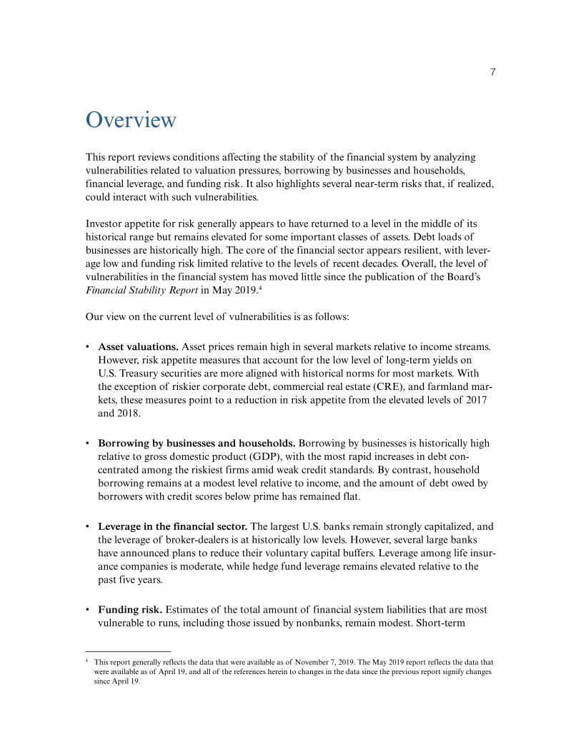
OverviewThis report reviews conditions affecting the stability of the financial system by analyzing vulner abilities related to valuation pressures, borrowing by businesses and households, financial leverage, and funding risk. It also highlights several near-term risks that, if realized, could interact with such vulnerabilities.

Investor appetite for risk generally appears to have returned to a level in the middle of its historical range but remains elevated for some important classes of assets. Debt loads of businesses are historically high. The core of the financial sector appears resilient, with lever-age low and funding risk limited relative to the levels of recent decades. Overall, the level of vulnerabilities in the financial system has moved little since the publication of the Board’s Financial Stability Report in May 2019.4

Our view on the current level of vulnerabilities is as follows:

• Asset valuations. Asset prices remain high in several markets relative to income streams. However, risk appetite measures that account for the low level of long-term yields on U.S. Treasury securities are more aligned with historical norms for most markets. With the exception of riskier corporate debt, commercial real estate (CRE), and farmland mar-kets, these measures point to a reduction in risk appetite from the elevated levels of 2017 and 2018.

• Borrowing by businesses and households. Borrowing by businesses is historically high relative to gross domestic product (GDP), with the most rapid increases in debt con-centrated among the riskiest firms amid weak credit standards. By contrast, household borrowing remains at a modest level relative to income, and the amount of debt owed by borrowers with credit scores below prime has remained flat.

• Leverage in the financial sector. The largest U.S. banks remain strongly capitalized, and the leverage of broker-dealers is at historically low levels. However, several large banks have announced plans to reduce their voluntary capital buffers. Leverage among life insur-ance companies is moderate, while hedge fund leverage remains elevated relative to the past five years.

• Funding risk. Estimates of the total amount of financial system liabilities that are most vulnerable to runs, including those issued by nonbanks, remain modest. Short-term

4 This report generally reflects the data that were available as of November 7, 2019. The May 2019 report reflects the data that were available as of April 19, and all of the references herein to changes in the data since the previous report signify changes since April 19.

8 oVerVIew

wholesale funding continues to be low compared with other liabilities, and the ratio of high-quality liquid assets to total assets remains high at large banks.

Stresses in Europe, such as those related to Brexit; stresses in emerging markets; and an unexpected and marked slowdown in U.S. economic growth are among the near-term risks that have the potential to interact with these vulnerabilities and pose risks to the financial system.

9

Valuation pressures remain elevated in some markets

Equity prices relative to forecast earnings remain above their long-run median, and yields on corporate bonds are near historically low levels. However, measures of investor appetite for risk that take into account the low level of long-term Treasury yields are broadly in line with historical norms for equity and safer corporate bonds, while they are still somewhat elevated for high-yield bonds and leveraged loans. CRE and farmland prices are elevated relative to rents and incomes in these sectors. By contrast, residential real estate (RRE) prices are roughly in line with their long-run relation to rents on a national basis.

Table 1 shows the size of the asset markets discussed in this section. The largest asset mar-kets are those for RRE, corporate equities, and CRE.

1.

Table 1. Size of Selected Asset Markets

ItemOutstanding

(billions of dollars)

Growth, 2018:Q2–2019:Q2

(percent)

Average annual growth, 1997–2019:Q2

(percent)

residential real estate 37,336 5.4 5.6

equities 35,624 5.5 8.9

Commercial real estate 20,030 5.1 7.5

Treasury securities 15,884 6.4 7.4

Investment-grade corporate bonds 5,864 5.4 8.4

Farmland 2,534 1.8 5.5

High-yield and unrated corporate bonds 1,317 .1 6.6

Leveraged loans* 1,197 14.6 15.4

Price growth (real)

Commercial real estate** 7.0 3.4

residential real estate*** 1.6 2.2

Note: The data extend through 2019:Q2. Growth rates are measured from Q2 of the year immediately preceding the period through Q2 of the final year of the period. equities, real estate, and farmland are at market value; bonds and loans are at book value.

* The amount outstanding shows institutional leveraged loans and generally excludes loan commitments held by banks. For example, lines of credit are generally excluded from this measure. average annual growth of leveraged loans is from 2000 to 2019:Q2, as this market was fairly small before then.

** one-year growth of commercial real estate prices is from June 2018 to June 2019, and average annual growth is from 1998:Q4 to 2019:Q2. Both growth rates are calculated from value-weighted nominal prices deflated using the consumer price index.

*** one-year growth of residential real estate is from June 2018 to June 2019, and average annual growth is from 1997:Q4 to 2019:Q2. Nominal prices are deflated using the consumer price index.

Source: For leveraged loans, S&P Global market Intelligence, Leveraged Commentary & Data; for corporate bonds, mergent, Inc., Corporate Fixed Income Securities Database; for farmland, Department of agriculture; for residential real estate price growth, CoreLogic; for commercial real estate price growth, CoStar Group, Inc., CoStar Commercial repeat Sale Indices (CCrSI); for all other items, Federal reserve Board, Sta-tistical release Z.1, “Financial accounts of the United States.”

Asset Valuations

10 aSSeT VaLUaTIoNS

1-3. option-Implied Volatility on the 10-Year Swap rate

Source: Barclays PLC, Barclays Live.

0

50

100

150

200

1999 2003 2007 2011 2015 2019

monthly

Basis points

Nov.

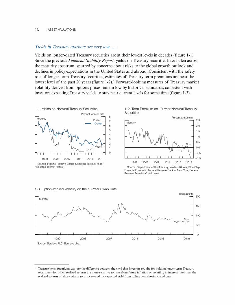
Yields in Treasury markets are very low . . .

Yields on longer-dated Treasury securities are at their lowest levels in decades (figure 1-1). Since the previous Financial Stability Report, yields on Treasury securities have fallen across the maturity spectrum, spurred by concerns about risks to the global growth outlook and declines in policy expectations in the United States and abroad. Consistent with the safety role of longer-term Treasury securities, estimates of Treasury term premiums are near the lowest level of the past 20 years (figure 1-2).5 Forward-looking measures of Treasury market volatility derived from options prices remain low by historical standards, consistent with investors expecting Treasury yields to stay near current levels for some time (figure 1-3).

5 Treasury term premiums capture the difference between the yield that investors require for holding longer-term Treasury securities—for which realized returns are more sensitive to risks from future inflation or volatility in interest rates than the realized returns of shorter-term securities—and the expected yield from rolling over shorter-dated ones.

0

1

2

3

4

5

6

7

8

1999 2003 2007 2011 2015 2019

monthly

Percent, annual rate

2-year10-year

Nov.

1-1. Yields on Nominal Treasury Securities

Source: Federal reserve Board, Statistical release H.15, “Selected Interest rates.”

−1.0

−0.5

0.0

0.5

1.0

1.5

2.0

2.5

1999 2003 2007 2011 2015 2019

monthly

Percentage points

Nov.

1-2. Term Premium on 10-Year Nominal Treasury Securities

Source: Department of the Treasury; wolters kluwer, Blue Chip Financial Forecasts; Federal reserve Bank of New York; Federal reserve Board staff estimates.


. . . as are yields on corporate bonds, while spreads on high-yield bonds remain somewhat compressed

Yields on corporate bonds are also very low, in line with very low Treasury yields (figure 1-4). The spread between yields on investment-grade corporate bonds and yields on Treasury securities is close to its long-run median.6 By contrast, the spread between yields on high-yield corporate bonds and yields on Treasury securities is narrower than its long-run median (figure 1-5). Other measures also suggest that investors’ appetite for riskier corporate bonds remains strong. For instance, the excess bond premium, measured as the gap between bond spreads and expected credit losses and inversely related to investor risk appetite, lies below its median (figure 1-6).7

6 Spreads between yields on corporate bonds and comparable-maturity Treasury securities reflect the extra compensation investors require to hold debt that is subject to corporate default or liquidity risks.

7 For a description of the excess bond premium, see Simon Gilchrist and Egon Zakrajšek (2012), “Credit Spreads and Busi-ness Cycle Fluctuations,” American Economic Review, vol. 102 (June), pp. 1692–720.

0

2

4

6

8

10

12

14

16

18

1999 2003 2007 2011 2015 2019

monthly

Percent

10-year high-yield

10-year triple-B

Nov.

1-4. Corporate Bond Yields

Source: ICe Data Indices, LLC, used with permission.

0

1

2

3

4

5

6

7

8

0

2

4

6

8

10

12

14

16

1999 2003 2007 2011 2015 2019

monthly

Percentage pointsPercentage points

Nov.

10-year triple-B(left scale)

10-yearhigh-yield(right scale)

1-5. Corporate Bond Spreads to Similar-maturity Treasury Securities

Source: ICe Data Indices, LLC, used with permission; Department of the Treasury.

1-6. Corporate Bond Premium over expected Losses

Source: Federal reserve Board staff calculations based on Lehman Brothers Fixed Income Database (warga); Intercontinental exchange, Inc., ICe Data Services; Center for research in Security Prices, CrSP/Compustat merged Database, wharton research Data Services; S&P Global market Intelligence, Compustat.

−3

−2

−1

0

1

2

3

4

5

1999 2003 2007 2011 2015 2019

monthly

Standard deviations from mean

oct.

12 aSSeT VaLUaTIoNS

Investor demand for leveraged loans remains strong, albeit below the levels seen in 2018. The interest rate spread on higher-rated leveraged loans is below its historical median, although the spread on lower-rated loans is close to its median and above the very tight level of last year, consistent with weakening demand for this class of loans (figure 1-7). Lending standards and loan covenants have gener-ally remained weak but have recently been tightening for lower-rated loans.

5

8

11

14

17

20

23

26

29

1994 1999 2004 2009 2014 2019

monthly

ratio

median

Nov.

1-8. Forward Price-to-earnings ratio of S&P 500 Firms

Source: Federal reserve Board staff calculations using refinitiv (formerly Thomson reuters), IBeS estimates.

−2

0

2

4

6

8

10

1994 1999 2004 2009 2014 2019

monthly

Percentage points

median

oct.

1-9. Spread of Forward earnings-to-Price ratio of S&P 500 Firms to 10-Year real Treasury Yield

Source: Federal reserve Board staff calculations using refinitiv (formerly Thomson reuters), IBeS estimates; Department of the Treasury; Survey of Professional Forecasters.

1.01.52.02.53.03.54.04.55.05.56.06.5

1999 2003 2007 2011 2015 2019

Percentage points

B+/BBB/BB−

monthly

Sept.

1-7. Spreads on Newly Issued Institutional Leveraged Loans

Source: S&P Global, Leveraged Commentary & Data.

Equity prices are high relative to corporate earnings, consistent with low interest rates

Over the past couple of years, equity prices have been high relative to forecasts of corporate earnings (figure 1-8). However, other measures of investors’ risk appetite in domestic equity markets are in the middle of their historical ranges. The gap between the forward earnings-to-price ratio and the expected real yield on 10-year Treasury securities—a rough measure of the premium investors require for holding corporate equities—is well above its long-run median (figure 1-9). A measure of expected equity return volatility over the next 30 days implied by option prices remains low (figure 1-10).


0

10

20

30

40

50

60

70

1999 2003 2007 2011 2015 2019

monthly average

Percent

option-implied volatility (VIX)realized volatility

Nov.

1-10. S&P 500 return Volatility

Source: Bloomberg Finance LP.

Liquidity in U.S. Treasury and equity futures markets deteriorated

“Market liquidity” refers to the cost of buying or selling securities quickly. Market liquidity conditions deteriorated in U.S. Treasury and equity futures markets amid separate episodes of elevated volatility in May and August. The box “What Has Been Happening to the Liquidity of U.S. Treasury and Equity Futures Markets?” provides additional information about these developments.

CRE prices are high relative to rents . . .

CRE prices have increased substantially over the past seven years (figure 1-11). By contrast, commercial property rents have generally risen more slowly. As a result, capitalization rates, which measure annual rental income relative to prices for recently transacted commercial properties, have moved down over the past decade and are at historically low levels, little changed since mid-2017 (figure 1-12). This year, the spread of capitalization rates over yields

5.5

6.0

6.5

7.0

7.5

8.0

8.5

9.0

9.5

10.0

2003 2007 2011 2015 2019

monthly

Percent

Sept.

1-12. Capitalization rate at Property Purchase

Source: real Capital analytics; andrew C. Florance, Norm G. miller, ruijue Peng, and Jay Spivey (2010), “Slicing, Dicing, and Scoping the Size of the U.S. Commercial real estate market,” Journal of Real Estate Portfolio Management, vol. 16 (may–august), pp. 101–18.

1-11. Commercial real estate Prices (real)

Source: CoStar Group, Inc., CoStar Commercial repeat Sale Indices; Bureau of Labor Statistics, consumer price index, via Haver analytics.

40

60

80

100

120

140

160

180

200

1999 2003 2007 2011 2015 2019

Jan. 2001 = 100

equal-weightedValue-weighted

monthly

Sept.

14 aSSeT VaLUaTIoNS

What Has Been Happening to the Liquidity of U.S. Treasury and Equity Futures Markets?

“Market liquidity” refers to the cost of quickly buying or selling a desired quantity of a security. Liquid markets support financial stability. Poor market liquidity exacerbates price volatility and may hinder the ability of investors and institutions to adjust positions, adversely affecting the ability of the financial system to adjust to shocks. In this discussion, we examine how liquid markets currently are, how frag-ile this liquidity is, and whether the risk of “flash events”—sudden, large changes in asset prices that are then reversed—has increased. We focus on two important markets: the interdealer U.S. Treasury security market and the E-mini S&P 500 futures market.

U.S. Treasury and equity futures market liquidity has recently deteriorated

Measuring market liquidity is challenging because liquidity has several dimensions. Some measures that capture different dimensions of market liquidity include the bid-ask spread, quoted depth, and price impact. The bid-ask spread is the difference between the best price offer to buy a security, which is the “bid,” and the best price offer to sell, which is the “ask.” In very competitive and liquid markets, the spread, or difference between the bid and ask prices, is small. Quoted depth is the quantity of an asset available to buy or sell at the posted bid and offer prices. Markets that are more liquid have greater quoted depth. Price impact is how much a security price changes for a given amount bought or sold. Markets are liquid when traders can sell larger quantities without triggering outsized price drops. For simplicity, the following analysis combines these three measures into a single index of illiquidity, which is higher when bid-ask spreads are wider, quoted depth is smaller, and trades have a greater effect on price.1

Figure A shows the illiquidity index for 2-, 5-, and 10-year U.S. Treasury notes from 2005 to the present, along with the Merrill Lynch Option Volatility Estimate, or MOVE, index, a measure of implied interest rate volatility. Illiquidity increased notably during the financial crisis and quickly declined there-after. Illiquidity also rose around the 2013 taper tantrum and the October 15, 2014, flash rally as well as in August 2019. In other words, Treasury security illiquidity is higher when Treasury yields are more volatile. This relationship holds true in most markets. To the extent that asset price volatility reflects

1 The indexes are calculated for each market as the first principal components of the standardized individual liquidity measures. The first principal components capture 60 to 85 percent of the variation in the individual measures.

(continued)

−3

0

3

6

9

12

0

60

120

180

240

2005 2007 2009 2011 2013 2015 2017 2019

Index pointsIndex points

Sept.30

Daily

Tapertantrum

Flashrally

Illiquidity index (left scale)moVe index (right scale)

Source: Staff calculations based on data from the interdealer broker community.

Figure a. U.S. Treasury Securities market Illiquidity Index


asset value uncertainty and the riskiness of providing liquidity, intermediaries either need to pull back as a way of managing the risk or need to charge more for providing liquidity as compensation for bear-ing the risk. This withdrawal and the increase in compensation for risk make trading more expensive, increasing illiquidity. Nonetheless, the relationship between U.S. Treasury illiquidity and interest rate volatility seems roughly stable over time, suggesting that liquidity has not become more fragile.

Figure B shows the illiquidity index for the E-mini S&P 500 futures contract, along with the CBOE Vol-atility Index (VIX). Illiquidity spiked during the financial crisis and, more recently, rose in early 2018, late 2018, and August 2019, coinciding with increases in the VIX. As with Treasury securities, equity illiquid-ity is higher when asset price volatility is higher. In contrast to U.S. Treasury securities, the relationship between the two appears to have changed since 2018, with illiquidity since then unusually high relative to its past relationship to volatility. This change suggests that liquidity has become more fragile over time—it tends to disappear when it is needed the most, when asset price volatility is high.

Flash events appear to have become modestly more frequent in equity futures

A possible implication of a deterioration in market liquidity is a greater incidence of flash events, in which prices move abruptly and sizably and then quickly revert. Indeed, such flash events have received significant attention from the press in recent years. Flash events may undermine confidence in trading venues and financial markets even if the price dislocations are short lived. Price dislocations, particularly if they occur at the end of a trading session, could trigger mark-to-market losses among a range of market participants. Finally, trading is increasingly connected across markets, so flash events in one market could affect trading and liquidity in other markets.

As shown in figure C, the number of flash events rose sharply during the crisis and then quickly declined. Recently, the number of flash events increased modestly in equity futures (the red bars) but not in the Treasury market (the blue bars).2

2 we identify flash events as five-minute returns that exceed 10 standard deviations in magnitude (positive or negative, based on all five-minute returns from 2005 to the present) and that then revert by at least two-thirds of the size of the initial jump within the next 12 hours.

(continued on next page)

Figure B. equity Futures market Illiquidity Index

Source: Staff calculations, based on data from Thomson reuters Tick History.

−3

0

3

6

9

0

20

40

60

80

2005 2007 2009 2011 2013 2015 2017 2019

PercentIndex points

Sept.30

Daily Illiquidity index (left scale)CBoe VIX (right scale)

16 aSSeT VaLUaTIoNS

To learn more, we asked dealers for their opinions

The September 2019 Senior Credit Officer Opinion Survey on Dealer Financing Terms asked dealers whether equity futures market liquidity has increased or decreased, on average, or become more fragile, in addition to inquiring about the causes of any changes. Consistent with the evidence shown in this discussion, dealers responded that, compared with January 2018, liquidity in the equity futures market has deteriorated and become more fragile. Survey respondents cited several reasons, includ-ing higher volatility, decreased willingness of principal trading firms (PTFs) and non-PTFs to provide liquidity, and an increase in the concentration of firms that provide liquidity.3 The box “Salient Shocks to Financial Stability Cited in Market Outreach” discusses other shifts in market structure that could render market liquidity more vulnerable to shocks.

3 a PTF is defined as a principal investor who deploys proprietary low-latency automated trading strategies and who may be registered as a broker-dealer but does not have clients as in a typical broker-dealer business model; see U.S. Department of the Treasury, Board of Governors of the Federal reserve System, Federal reserve Bank of New York, U.S. Securities and exchange Commission, and U.S. Commodity Futures Trading Commission (2015), Joint Staff Report: The U.S. Treasury Market on October 15, 2014 (washing-ton: Department of the Treasury, Board of Governors, FrBNY, SeC, and CFTC, July), https://www.treasury.gov/press-center/press-releases/Documents/Joint_Staff_report_Treasury_10-15-2015.pdf.

Figure C. Flash events

0

10

20

30

40

50Number of jumpsNumber of jumps

2005 2006 2007 2008 2009 2010 2011 2012 2013 2014 2015 2016 2017 2018 2019

0

3

6

9

12

15

U.S. Treasury securities (left scale)equity futures (right scale)

Source: Staff calculations based on data from the interdealer broker community and Thomson reuters Tick History.

What Has Been Happening to Market Liquidity? (continued)

https://www.treasury.gov/press-center/press-releases/Documents/Joint_Staff_Report_Treasury_10-15-2015.pdf

https://www.treasury.gov/press-center/press-releases/Documents/Joint_Staff_Report_Treasury_10-15-2015.pdf


on 10-year Treasury securities, which is a rough measure of the premium that investors require for holding CRE over safe alternative investments, has risen from low levels to above its median over the past decade, as the decline in Treasury yields this year has not been accompanied by an acceleration in CRE prices (figure 1-13). Data from the Senior Loan Officer Opinion Survey on Bank Lending Practices (SLOOS) collected in July and October indicated that CRE lending standards were tightened, on net, in the second and third quarters (figure 1-14). They remained at the tighter end of the range that has prevailed since 2005.

. . . and farmland prices are falling from recent historical highs . . .

Although they have recently moved down from their peaks, farmland prices, both nationally and in several midwestern states, remain high by historical standards (figure 1-15). Farmland prices also remain high relative to rents (figure 1-16). Net farm income continues to be well below the high levels seen in the early years of the past decade, reflecting low agricultural commodity prices and trade tensions.

1-13. Spread of Capitalization rate at Property Purchase to 10-Year Treasury Yield

Source: real Capital analytics; andrew C. Florance, Norm G. miller, ruijue Peng, and Jay Spivey (2010), “Slicing, Dicing, and Scoping the Size of the U.S. Commercial real estate market,” Journal of Real Estate Portfolio Management, vol. 16 (may–august), pp. 101–18; Department of the Treasury.

1.01.52.02.53.03.54.04.55.05.56.0

2003 2007 2011 2015 2019

Percentage points

Sept.

monthly

median

−100−80−60−40−20

020406080

100

1999 2003 2007 2011 2015 2019

Quarterly

Net percentage of banks reporting

eas

ing

Ti

ghte

ning

Q3

1-14. Change in Bank Standards for Cre Loans

Source: Federal reserve Board, Senior Loan officer opinion Survey on Bank Lending Practices; Federal reserve Board staff calculations.

1-15. Farmland Prices

Source: Department of agriculture; Federal reserve Board staff calculations.

1000

2000

3000

4000

5000

6000

7000

1969 1979 1989 1999 2009 2019

annual

2018 dollars per acre

median

midwest indexUnited States

1-16. Farmland Price-to-rent ratio

Source: Department of agriculture; Federal reserve Board staff calculations.

10

15

20

25

30

35

1969 1979 1989 1999 2009 2019

annual

ratio

median

midwest indexUnited States

18 aSSeT VaLUaTIoNS

. . . while home prices are growing moderately and are consistent with rents

House prices have risen substantially since 2012, although increases in home prices have slowed noticeably this year and, nationwide, recent levels of home prices appear broadly in line with rents (figure 1-17). For instance, while the aggregate housing price-to-rent ratio is higher than its long-run historical trend, this implied gap is small (figure 1-18). How-ever, housing price-to-rent ratios vary significantly across regional markets, and price-to-rent ratios for cities that have seen rapid price increases are still above their usual ranges ( figure 1-19).

60

70

80

90

100

110

120

130

140

150

1983 1989 1995 2001 2007 2013 2019

monthly

Trend at Sept. 2019 = 100

Price-to-rent ratio

Long-run trend

Sept.

1-18. Housing Price-to-rent ratio

Source: For house prices, CoreLogic; for rent data, Bureau of Labor Statistics.

−15

−10

−5

0

5

10

15

20

2011 2013 2015 2017 2019

monthly

12−month percent change

ZillowCoreLogic

Sept.

1-17. Growth of Nominal Prices of existing Homes

Source: CoreLogic; Zillow.

1-19. Selected Local Housing Price-to-rent ratio Indexes

406080

100120140160180200220240

1991 1993 1995 1997 1999 2001 2003 2005 2007 2009 2011 2013 2015 2017 2019

monthly

Jan. 2010 = 100

Sept.

PhoenixmiamiLos angelesmedianmiddle 80% of markets

Source: For house prices, CoreLogic; for rent data, Bureau of Labor Statistics.

19

Business-sector debt relative to GDP is historically high amid weak credit standards, whereas debt owed by households remains at a modest level relative to incomes

On balance, vulnerabilities arising from total private-sector credit are at moderate levels. Business debt levels are high compared with either business assets or GDP, with the riskiest firms accounting for most of the increase in debt in recent years. By contrast, household borrowing has advanced more slowly than economic activity and has been heavily concen-trated among borrowers with high credit scores.

Table 2 shows the current volume and recent historical growth rates of forms of debt owed by nonfinancial businesses and households. Total outstanding private credit is split equally among businesses and households, with each owing close to $16 trillion.

2.

Table 2. Outstanding Amounts of Nonfinancial Business and Household Credit

ItemOutstanding


Growth, 2018:Q2–2019:Q2

(percent)


(percent)

Total private nonfinancial credit 31,530 4.1 5.5

Total business credit 15,764 5.1 5.7

Corporate business credit 9,973 4.7 5.1

Bonds and commercial paper 6,499 3.6 5.7

Bank lending 1,409 6.5 2.9

Leveraged loans* 1,137 14.6 15.4

Noncorporate business credit 5,791 5.6 7.2

Commercial real estate 2,431 4.5 6.2

Total household credit 15,766 3.2 5.4

mortgages 10,415 2.7 5.5

Consumer credit 4,057 5.1 5.2

Student loans 1,607 5.1 9.3

auto loans 1,173 3.9 5.0

Credit cards 1,031 4.0 3.1

Nominal GDP 21,339 4.6 4.2

Note: The data extend through 2019:Q2. Growth rates are measured from Q2 of the year immediately preceding the period through Q2 of the final year of the period. The table reports the main components of corporate business credit, total household credit, and consumer credit. other, smaller components are not reported. The commercial real estate (Cre) row shows Cre debt owed by both corporate and noncorporate busi-nesses. The total household sector credit includes debt owed by other entities, such as nonprofit organizations. GDP is gross domestic product.

* Leveraged loans included in this table are an estimate of the leveraged loans that are made to nonfinancial businesses only and do not include the small amount of leveraged loans outstanding for financial businesses. The amount outstanding shows institutional leveraged loans and generally excludes loan commitments held by banks. For example, lines of credit are generally excluded from this measure. The average annual growth rate shown for leveraged loans is computed from 2000 to 2019:Q2, as this market was fairly small before 2000.

Source: For leveraged loans, S&P Global, Leveraged Commentary & Data; for GDP, Bureau of economic analysis, national income and product accounts; for all other items, Federal reserve Board, Statistical release Z.1, “Financial accounts of the United States.”

Borrowing by Businesses and Households

20 BorrowING BY BUSINeSSeS aND HoUSeHoLDS

Figure 2-2 shows the credit-to-GDP ratio separately for the household and nonfinancial business sectors (leverage of financial firms is discussed in the next section). Before the crisis, household debt relative to GDP rose steadily to levels far above historical trends. After the crisis, the household debt-to-GDP ratio fell sharply and has leveled off since then. Business borrowing tends to track the economic cycle more closely. After the crisis, the business debt-to-GDP ratio also fell but has expanded significantly over the past several years and is now near its historical high.

Total private credit has advanced roughly in line with economic activity . . .

Over the past several years, total debt owed by businesses and households expanded at a pace similar to that of nominal GDP. As a result, the nonfinancial-sector credit-to-GDP ratio has been broadly stable, similar to its level in mid-2005, the period preceding the most rapid credit growth from 2006 to 2007 (figure 2-1).

2-2. Nonfinancial Business- and Household-Sector Credit-to-GDP ratios

0.3

0.4

0.5

0.6

0.7

0.8

0.9

1.0

1.1

0.45

0.50

0.55

0.60

0.65

0.70

0.75

1983 1986 1989 1992 1995 1998 2001 2004 2007 2010 2013 2016 2019

Quarterly

ratioratio

Nonfinancial business (right scale)Household (left scale)

Q2

Source: Federal reserve Board staff calculations based on Bureau of economic analysis, national income and product accounts, and Federal reserve Board, Statistical release Z.1, “Financial accounts of the United States.”

2-1. Private Nonfinancial-Sector Credit-to-GDP ratio

0.8

1.1

1.4

1.7

2.0

1980 1983 1986 1989 1992 1995 1998 2001 2004 2007 2010 2013 2016 2019

Quarterly

ratio

Q2

Source: Federal reserve Board staff calculations based on Bureau of economic analysis, national income and product accounts, and Federal reserve Board, Statistical release Z.1, “Financial accounts of the United States.”


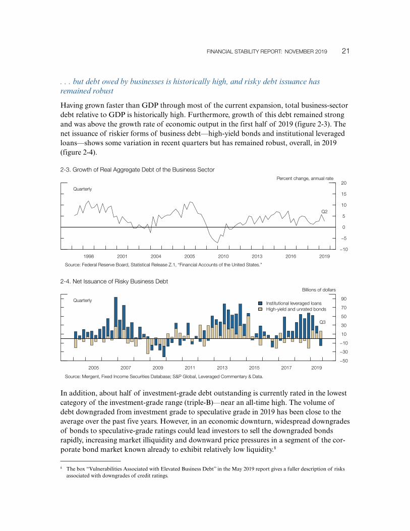
. . . but debt owed by businesses is historically high, and risky debt issuance has remained robust

Having grown faster than GDP through most of the current expansion, total business-sector debt relative to GDP is historically high. Furthermore, growth of this debt remained strong and was above the growth rate of economic output in the first half of 2019 (figure 2-3). The net issuance of riskier forms of business debt—high-yield bonds and institutional leveraged loans—shows some variation in recent quarters but has remained robust, overall, in 2019 (figure 2-4).

2-4. Net Issuance of risky Business Debt

−50

−30

−10

10

30

50

70

90

2005 2007 2009 2011 2013 2015 2017 2019

Quarterly

Billions of dollars

Q3

Institutional leveraged loansHigh-yield and unrated bonds

Source: mergent, Fixed Income Securities Database; S&P Global, Leveraged Commentary & Data.

In addition, about half of investment-grade debt outstanding is currently rated in the lowest category of the investment-grade range (triple-B)—near an all-time high. The volume of debt downgraded from investment grade to speculative grade in 2019 has been close to the average over the past five years. However, in an economic downturn, widespread downgrades of bonds to speculative-grade ratings could lead investors to sell the downgraded bonds rapidly, increasing market illiquidity and downward price pressures in a segment of the cor-porate bond market known already to exhibit relatively low liquidity.8

8 The box “Vulnerabilities Associated with Elevated Business Debt” in the May 2019 report gives a fuller description of risks associated with downgrades of credit ratings.

−10

−5

0

5

10

15

20

1998 2001 2004 2005 2010 2013 2016 2019

Quarterly

Percent change, annual rate

Q2

2-3. Growth of real aggregate Debt of the Business Sector

Source: Federal reserve Board, Statistical release Z.1, “Financial accounts of the United States.”

https://www.federalreserve.gov/publications/files/financial-stability-report-201905.pdf


Moreover, credit standards for some business loans remain weak . . .

In line with the discussion of price terms and risk appetite in section 1, demand for insti-tutional leveraged loans has remained strong and credit standards have remained weak. The share of newly issued loans to large corporations with high leverage—defined as those with ratios of debt to earnings before interest, taxes, depreciation, and amortization greater than 6—exceeds previous peak levels observed in 2007 and 2014 when underwriting quality was poor (figure 2-5). Incoming data point to continued strong issuance of leveraged loans in the third quarter of 2019. However, the credit performance of leveraged loans has been solid so far, with low default rates (figure 2-6).

. . . and balance sheet leverage of businesses is near its highest level over the past two decades

A broad indicator of the leverage of businesses—the ratio of debt to assets for all publicly traded nonfinancial firms—is at its highest level in 20 years (figure 2-7).9 Moreover, the

9 The dashed line in the series beginning in the first quarter of 2019 reflects a structural break due to a new accounting stan-dard that requires operating leases, previously considered off-balance-sheet activities, to be included in measures of debt and assets.


2-6. Default rates of Leveraged Loans

−2

0

2

4

6

8

10

12

14

2001 2004 2007 2010 2013 2016 2019

monthly

Percent

Sept.

2-5. Distribution of Institutional Leveraged Loan Volumes, by Debt-to-eBITDa ratio

0

20

40

60

80

100

120

140

160

2001 2004 2007 2010 2013 2016 2019

Percent

Debt multiples ≥ 6xDebt multiples 5x−5.99xDebt multiples 4x−4.99xDebt multiples < 4x Q3



leverage ratio among highly leveraged firms—defined as firms above the 75th percentile of the leverage distribution—is close to a historical high. Despite high balance sheet leverage, historically low interest rates have contributed to keeping the ratio of corporate earnings to interest expenses high for the median firm and near the historical median for riskier firms, which are those in the bottom 25th percentile of the distribution of this ratio (figure 2-8).

Borrowing by households, however, has risen in line with incomes and is concentrated among borrowers with low credit risk

Household debt continues to expand in line with income, but debt owed by households with prime ratings accounts for most of the growth. Loan balances owed by borrowers with a prime credit score, who account for about one-half of all borrowers and about two-thirds of all balances, continued to grow in the first half of 2019, surpassing pre-crisis levels (after an adjustment for general price inflation). By contrast, inflation-adjusted loan balances for the remaining one-half of borrowers with near-prime and subprime credit scores have changed little since 2014 (figure 2-9).

20

25

30

35

40

45

50

55

2001 2004 2007 2010 2013 2016 2019

Quarterly

Percent

75th percentile

all firmsQ2

2-7. Gross Balance Sheet Leverage of Public Nonfinancial Businesses

Source: Federal reserve Board staff calculations based on S&P Global, Compustat.

−1.0−0.50.00.51.01.52.02.53.03.54.04.5

2001 2004 2007 2010 2013 2016 2019

Quarterly

ratio

Q2

median25th percentile

2-8. Interest Coverage ratios for Public Nonfinancial Businesses

Source: Compustat.

100018002600340042005000580066007400820090009800

2001 2004 2007 2010 2013 2016 2019

Quarterly

Billions of dollars (real)

Q2

Prime

Q2

Near prime

Subprime

2-9. Total Household Loan Balances

Source: FrBNY Consumer Credit Panel/equifax; Bureau of Labor Statistics, consumer price index.


Credit risk of outstanding mortgages remains generally low . . .

Mortgage debt accounts for roughly two-thirds of total household credit. New mortgage extensions remain skewed toward prime borrowers, consistent with the general shift in the composition of household debt toward less-risky borrowers and in line with stronger under-writing standards relative to the mid-2000s (figure 2-10). Mortgage loan performance has been solid, resulting in low credit losses for lenders. An early indicator of payment difficul-ties is the rate at which existing mortgages transition into delinquency, and this rate has been low for several years among borrowers with prime and nonprime credit scores and for loans in programs offered by the Federal Housing Administration and the U.S. Department of Veterans Affairs (figure 2-11). Delinquency rates for newly originated mortgages, a gauge of recent underwriting standards, have been low as well. In addition, the ratio of outstanding mortgage debt to home values is now at the level seen in the relatively calm housing market of the late 1990s, suggesting that home mortgages are currently backed by sufficient collat-eral, thus providing lenders with protection against credit losses (figure 2-12). Also, the share

70

80

90

100

110

120

130

140

150

2001 2004 2007 2010 2013 2016 2019

Quarterly

1999:Q1 = 100

Q2

relative to model- implied values

relative to market value

2-12. estimates of Housing Leverage

Source: FrBNY Consumer Credit Panel/equifax; CoreLogic; Bureau of Labor Statistics.

0

1

2

3

4

5

6

7

2001 2004 2007 2010 2013 2016 2019

monthly

Percent of previously current loans

Nonprime

JulyFHa/VaPrime

2-11. Transition rates into mortgage Delinquency

Source: For prime and FHa/Va, Black knight mcDash Data; for nonprime, CoreLogic.

0

200

400

600

800

1000

1200

1400Billions of dollars (real)

2001 2004 2007 2010 2013 2016 2019

annual SubprimeNear primePrime

2-10. estimate of New mortgage Volume to Households



of outstanding mortgages with negative equity—mortgages where the amount owed on a property exceeds its underlying value—has continued to edge down (figure 2-13).

. . . although some households are struggling to manage their debt

The remaining one-third of total debt owed by households, commonly referred to as con-sumer credit, consists mainly of student loans, auto loans, and credit card debt (figure 2-14). Table 2 shows that consumer credit rose 5 percent over the year ending in the first quarter of 2019 and currently stands at about $4 trillion.

2-13. estimate of mortgages with Negative equity

Source: CoreLogic; Zillow.

0

10

20

30

40

2011 2013 2015 2017 2019

Percent

June

Q4

ZillowCoreLogic

Household balances on student loans continued their upward trajectory in the first half of 2019. Delinquency rates on those loans remain high relative to historical standards, although they have been, on balance, moving sideways in recent years. Although the risks posed to the broader financial system appear limited, as the majority of student loans were issued through government programs, the elevated student loan balances and delinquency rates highlight the challenges associated with debt payments some households continue to face.

200

400

600

800

1000

1200

1400

1600

1800

2001 2004 2007 2010 2013 2016 2019

Quarterly


Student loans

auto loans

Q2

Credit cards

2-14. Consumer Credit Balances



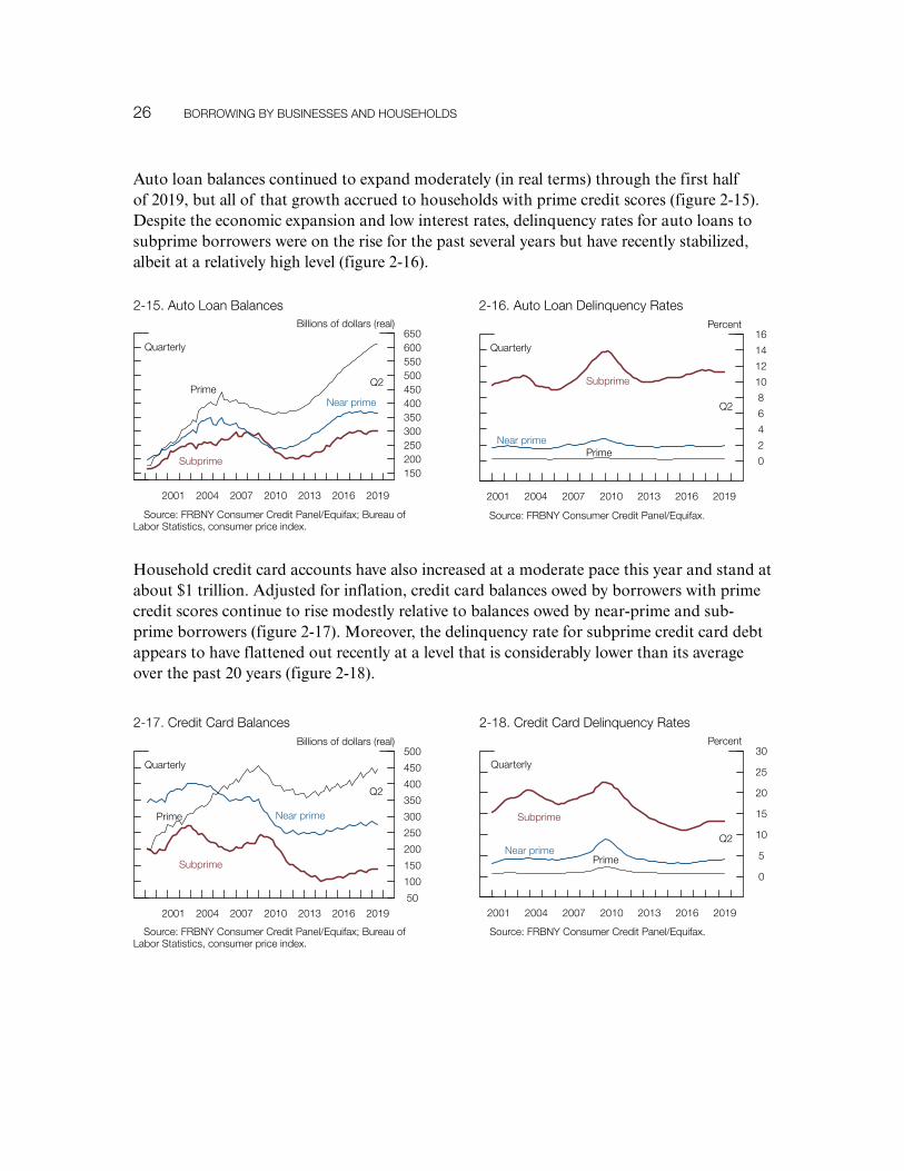
Auto loan balances continued to expand moderately (in real terms) through the first half of 2019, but all of that growth accrued to households with prime credit scores (figure 2-15). Despite the economic expansion and low interest rates, delinquency rates for auto loans to subprime borrowers were on the rise for the past several years but have recently stabilized, albeit at a relatively high level (figure 2-16).

50

100

150

200

250

300

350

400

450

500

2001 2004 2007 2010 2013 2016 2019

Quarterly


Prime

Q2

Near prime

Subprime

2-17. Credit Card Balances


0

5

10

15

20

25

30

2001 2004 2007 2010 2013 2016 2019

Quarterly

Percent

Prime

Q2Near prime

Subprime

2-18. Credit Card Delinquency rates

Source: FrBNY Consumer Credit Panel/equifax.

0

2

4

6

8

10

12

14

16

2001 2004 2007 2010 2013 2016 2019

Quarterly

Percent

Prime

Q2

Near prime

Subprime

2-16. auto Loan Delinquency rates

Source: FrBNY Consumer Credit Panel/equifax.

150200250300350400450500550600650

2001 2004 2007 2010 2013 2016 2019

Quarterly


PrimeQ2

Near prime

Subprime

2-15. auto Loan Balances


Household credit card accounts have also increased at a moderate pace this year and stand at about $1 trillion. Adjusted for inflation, credit card balances owed by borrowers with prime credit scores continue to rise modestly relative to balances owed by near-prime and sub-prime borrowers (figure 2-17). Moreover, the delinquency rate for subprime credit card debt appears to have flattened out recently at a level that is considerably lower than its average over the past 20 years (figure 2-18).

27

3.

Table 3. Size of Selected Sectors of the Financial System, by Types of Institutions and Vehicles

ItemTotal assets


Growth, 2018:Q2–2019:Q2

(percent)


(percent)

Banks and credit unions 19,506 3.1 5.7

mutual funds 16,670 3.7 10.2

Insurance companies 10,730 6.3 6.1

Life 8,149 5.9 6.2

Property and casualty 2,581 7.3 5.8

Hedge funds* 7,593 4.8 7.2

Broker-dealers 3,487 11.1 5.1

Outstanding (billions of dollars)

Securitization 10,402 3.0 5.4

agency 9,243 3.4 5.9

Non-agency** 1,159 − .3 3.0

Note: The data extend through 2019:Q2. Growth rates are measured from Q2 of the year immediately preceding the period through Q2 of the final year of the period. Life insurance companies’ assets include both general and separate account assets.

* Hedge fund data start in 2013:Q4 and are updated through 2018:Q4.** Non-agency securitization excludes securitized credit held on balance sheets of banks and finance companies.Source: Federal reserve Board, Statistical release Z.1, “Financial accounts of the United States”; Federal reserve Board staff calculations

based on Securities and exchange Commission, Form PF, reporting Form for Investment advisers to Private Funds and Certain Commodity Pool operators and Commodity Trading advisors.

Current debt levels point to financial-sector resilience

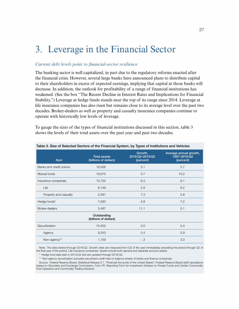
The banking sector is well capitalized, in part due to the regulatory reforms enacted after the financial crisis. However, several large banks have announced plans to distribute capital to their shareholders in excess of expected earnings, implying that capital at those banks will decrease. In addition, the outlook for profitability of a range of financial institutions has weakened. (See the box “The Recent Decline in Interest Rates and Implications for Financial Stability.”) Leverage at hedge funds stands near the top of its range since 2014. Leverage at life insurance companies has also risen but remains close to its average level over the past two decades. Broker-dealers as well as property and casualty insurance companies continue to operate with historically low levels of leverage.

To gauge the sizes of the types of financial institutions discussed in this section, table 3 shows the levels of their total assets over the past year and past two decades.

Leverage in the Financial Sector

28 LeVeraGe IN THe FINaNCIaL SeCTor

The Recent Decline in Interest Rates and Implications for Financial Stability

In line with sovereign yields globally, yields on U.S. Treasury securities have declined substantially over the past year, in part reflecting decisions by the Federal Open Market Committee designed to keep the U.S. economy strong. However, yields at longer maturities have fallen more than those at some shorter maturities. Market equity-to-book ratios for some financial intermediaries have fallen over recent quarters. If interest rates were to remain low for a prolonged period, the profitability of banks, insurers, and other financial intermediaries could come under stress and spur reach-for-yield behavior, thereby increasing the vulnerability of the financial sector to subsequent shocks.

To be sure, the profitability of banks is currently strong. However, the fall in long-term interest rates has the potential to compress net interest margins and thus weaken the profitability of banks. The interest rates that banks earn on loans are typically set at a spread over an interest rate benchmark and are therefore likely to come down as benchmark rates decline. By contrast, the interest rates that banks pay to depositors are already quite low and unlikely to decline much further. Taken together, falling loan rates and largely unchanged deposit rates could compress the net interest income of banks. Moreover, the pressures on profitability among banks could encourage reach-for-yield behavior, including an ero-sion of lending standards and an increased willingness to extend credit to firms with weaker balance sheets and households with lower credit ratings.

A decrease in interest rates can also weaken the profitability outlook for life insurance companies by affecting both their assets and their liabilities. Life insurance companies hold asset portfolios of long-term fixed-income securities to back the stream of payments on even longer-term insurance liabilities. Falling interest rates tend to induce policyholders to surrender their contracts less frequently because new policies will likely offer lower rates than existing policies. In addition, low rates can reduce the yield insurers earn on their assets, as higher-yielding assets gradually mature and are replaced with lower-yielding ones.

Low interest rates may also increase risk-taking among some financial institutions. In addition to the pressures on banks and insurance companies, low interest rates could affect pension funds and other institutional investors who offer pre-specified returns for policyholders that are significantly higher than the general level of interest rates. In order to meet the specified yield, these asset managers may hold riskier investment portfolios, which are expected to generate higher returns. Furthermore, this decision could artificially increase the price of risky assets.

While vulnerabilities related to low interest rates have the potential to grow, thus calling for caution and continued monitoring, so far, the financial system appears resilient.


Banks are well capitalized

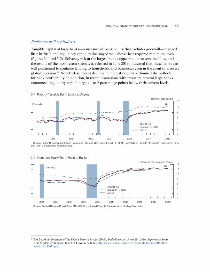
Tangible capital at large banks—a measure of bank equity that excludes goodwill—changed little in 2019, and regulatory capital ratios stayed well above their required minimum levels (figures 3-1 and 3-2). Solvency risk at the largest banks appears to have remained low, and the results of the most recent stress test, released in June 2019, indicated that these banks are well positioned to continue lending to households and businesses even in the event of a severe global recession.10 Nonetheless, recent declines in interest rates have dimmed the outlook for bank profitability. In addition, in recent discussions with investors, several large banks announced regulatory capital targets 1 to 2 percentage points below their current levels.

10 See Board of Governors of the Federal Reserve System (2019), Dodd-Frank Act Stress Test 2019: Supervisory Stress Test Results (Washington: Board of Governors, June), https://www.federalreserve.gov/publications/files/2019-dfast-results-20190621.pdf.

0

2

4

6

8

10

12

1989 1994 1999 2004 2009 2014 2019

Quarterly

Percent of total assets

other BHCsLarge non–G-SIBsG-SIBs

Q2

3-1. ratio of Tangible Bank equity to assets

Source: Federal Financial Institutions examination Council, Call report Form FFIeC 031, Consolidated reports of Condition and Income for a Bank with Domestic and Foreign offices.

0

2

4

6

8

10

12

14

2001 2003 2005 2007 2009 2011 2013 2015 2017 2019

Quarterly

Percent of risk−weighted assets

other BHCsLarge non−G-SIBsG-SIBs

Q2

3-2. Common equity Tier 1 ratio of Banks

Source: Federal reserve Board, Form Fr Y-9C, Consolidated Financial Statements for Holding Companies.

https://www.federalreserve.gov/publications/files/2019-dfast-results-20190621.pdf

https://www.federalreserve.gov/publications/files/2019-dfast-results-20190621.pdf


Leverage stayed low at broker-dealers and remained moderate at life insurance companies . . .

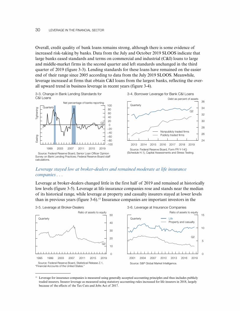
Leverage at broker-dealers changed little in the first half of 2019 and remained at historically low levels (figure 3-5). Leverage at life insurance companies rose and stands near the median of its historical range, while leverage at property and casualty insurers stayed at lower levels than in previous years (figure 3-6).11 Insurance companies are important investors in the

11 Leverage for insurance companies is measured using generally accepted accounting principles and thus includes publicly traded insurers. Insurer leverage as measured using statutory accounting rules increased for life insurers in 2018, largely because of the effects of the Tax Cuts and Jobs Act of 2017.

Overall, credit quality of bank loans remains strong, although there is some evidence of increased risk-taking by banks. Data from the July and October 2019 SLOOS indicate that large banks eased standards and terms on commercial and industrial (C&I) loans to large and middle-market firms in the second quarter and left standards unchanged in the third quarter of 2019 (figure 3-3). Lending standards for these loans have remained on the easier end of their range since 2005 according to data from the July 2019 SLOOS. Meanwhile, leverage increased at firms that obtain C&I loans from the largest banks, reflecting the over-all upward trend in business leverage in recent years (figure 3-4).

3-6. Leverage at Insurance Companies

Source: S&P Global market Intelligence.

0

5

10

15

2001 2004 2007 2010 2013 2016 2019

Quarterly

ratio of assets to equity

LifeProperty and casualty

Q2

3-5. Leverage at Broker-Dealers

Source: Federal reserve Board, Statistical release Z.1, “Financial accounts of the United States.”

0

10

20

30

40

50

1995 1999 2003 2007 2011 2015 2019

Quarterly

ratio of assets to equity

Q2

24

26

28

30

32

34

36

2013 2014 2015 2016 2017 2018 2019

Quarterly

Debt as percent of assets

Q2

Nonpublicly traded firmsPublicly traded firms

3-4. Borrower Leverage for Bank C&I Loans

Source: Federal reserve Board, Form Fr Y-14Q (Schedule H.1), Capital assessments and Stress Testing.

−100−80−60−40−20

020406080

100

1999 2003 2007 2011 2015 2019

Quarterly

Net percentage of banks reporting

eas

ing

Tig

hten

ing

Q3

3-3. Change in Bank Lending Standards for C&I Loans

Source: Federal reserve Board, Senior Loan officer opinion Survey on Bank Lending Practices; Federal reserve Board staff calculations.


corporate bond and collateralized loan obligation (CLO) markets, exposing them to risks stemming from elevated leverage in the corporate sector. However, the modest level of lever-age at insurance companies should help limit the amplification of possible shocks emanating from the business sector.

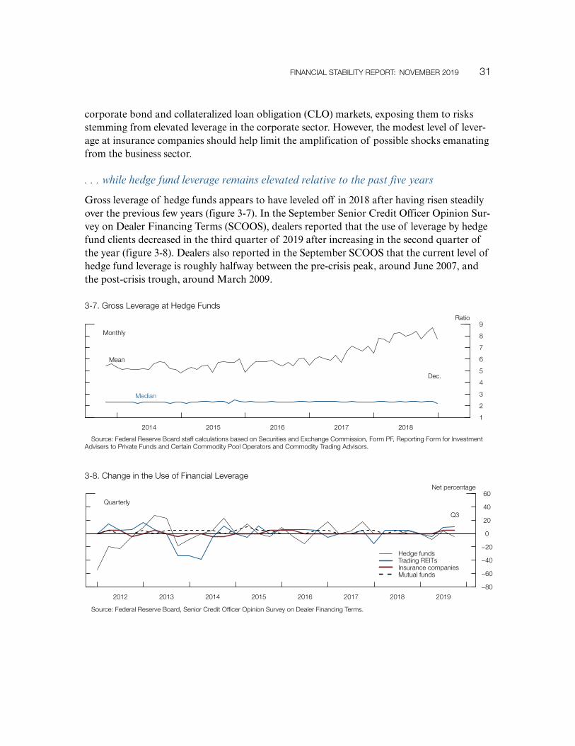
. . . while hedge fund leverage remains elevated relative to the past five years

Gross leverage of hedge funds appears to have leveled off in 2018 after having risen steadily over the previous few years ( figure 3-7). In the September Senior Credit Officer Opinion Sur-vey on Dealer Financing Terms (SCOOS), dealers reported that the use of leverage by hedge fund clients decreased in the third quarter of 2019 after increasing in the second quarter of the year (figure 3-8). Dealers also reported in the September SCOOS that the current level of hedge fund leverage is roughly halfway between the pre-crisis peak, around June 2007, and the post-crisis trough, around March 2009.

1

2

3

4

5

6

7

8

9

2014 2015 2016 2017 2018

monthly

ratio

mean

median

Dec.

3-7. Gross Leverage at Hedge Funds

Source: Federal reserve Board staff calculations based on Securities and exchange Commission, Form PF, reporting Form for Investment advisers to Private Funds and Certain Commodity Pool operators and Commodity Trading advisors.

−80

−60

−40

−20

0

20

40

60

2012 2013 2014 2015 2016 2017 2018 2019

Quarterly

Net percentage

Hedge fundsTrading reITsInsurance companiesmutual funds

Q3

3-8. Change in the Use of Financial Leverage

Source: Federal reserve Board, Senior Credit officer opinion Survey on Dealer Financing Terms.


Securitization volumes were largely unchanged . . .

Securitization allows financial institutions to bundle loans or other financial assets and sell claims on the cash flows generated by these assets as securities that can be traded, much like bonds. This process often involves the creation of claims with different levels of seniority and thus represents a form of credit risk transformation, whereby highly rated securities can be created from a pool of lower-rated underlying assets. Examples of the resulting securities include CLOs, asset-backed securities, and commercial and residential mortgage-backed securities. Issuance volumes of non-agency securities (that is, those not guaranteed by a government-sponsored enterprise or by the federal government) remain well below the levels seen in the run-up to the financial crisis (figure 3-9).

0

400

800

1200

1600

2000

2400

2800

2001 2003 2005 2007 2009 2011 2013 2015 2017 2019

annual


otherPrivate-label rmBSNon-agency CmBSauto loan/lease aBSCDos (incl. aBS, CDo, and CLo)

3-9. Issuance of Non-agency Securitized Products, by asset Class

Source: Harrison Scott Publications, asset-Backed alert (aBalert.com) and Commercial mortgage alert (Cmalert.com); Bureau of Labor Statistics, consumer price index, via Haver analytics.

CLO issuance has increased rapidly since 2012 and continues to be robust in 2019 after reaching a record level in 2018. These securities fund more than 50 percent of outstanding institutional leveraged loans. Unlike open-end mutual funds, CLOs do not generally permit early redemptions and do not rely on funding that must be rolled over before the underlying assets mature. As a result, CLOs avoid run risk associated with a rapid reversal in investor sentiment.

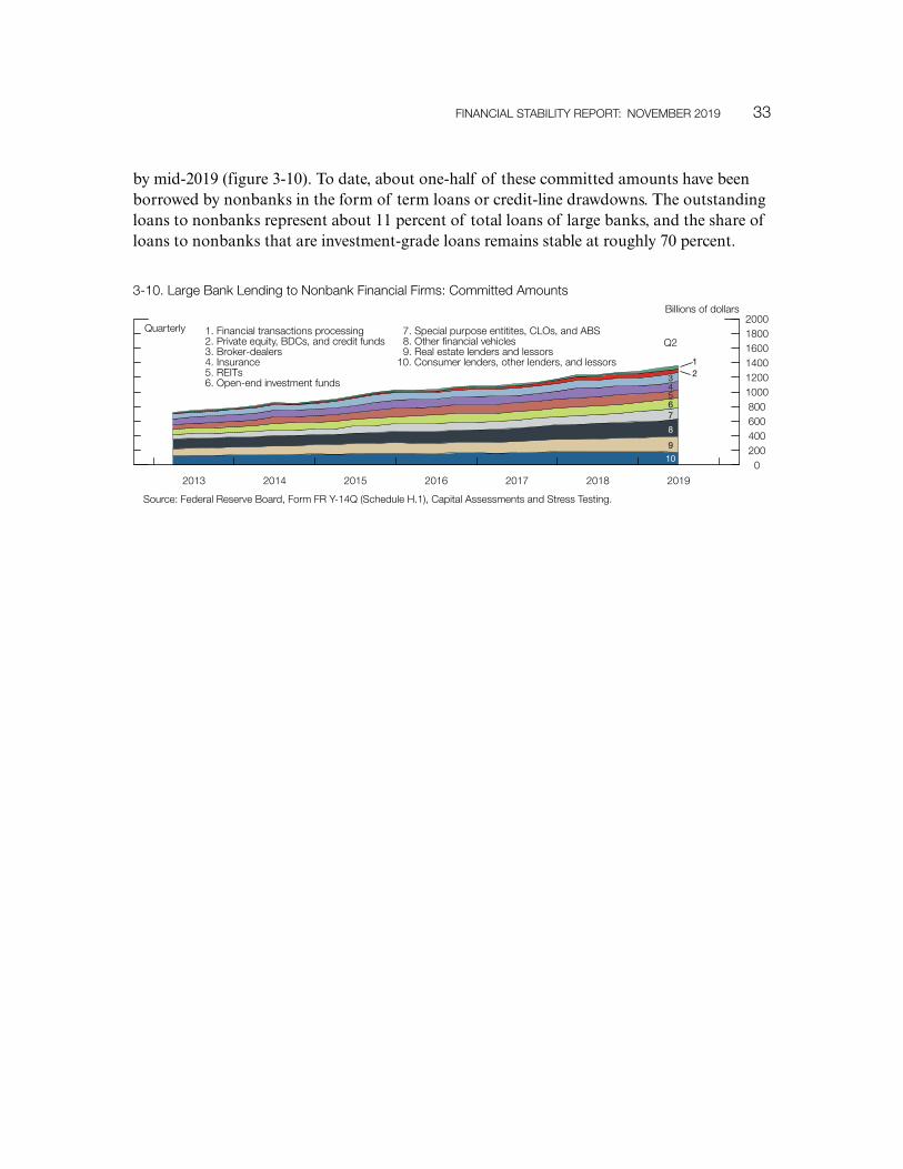
. . . while bank lending to nonbank financial institutions continued to grow notably

Data on bank lending to financial institutions operating outside the banking sector—such as finance companies, asset managers, securitization vehicles, and mortgage real estate investment trusts—can be informative about the use of leverage by nonbanks and shed light on the credit exposures of banks to these institutions. Committed amounts of credit from large banks to nonbanks have nearly doubled since 2013 and reached about $1.4 trillion


by mid-2019 (figure 3-10). To date, about one-half of these committed amounts have been borrowed by nonbanks in the form of term loans or credit-line drawdowns. The outstanding loans to nonbanks represent about 11 percent of total loans of large banks, and the share of loans to nonbanks that are investment-grade loans remains stable at roughly 70 percent.

Quarterly

Billions of dollars

0200400600800

100012001400160018002000

2013 2014 2015 2016 2017 2018 2019

1. Financial transactions processing2. Private equity, BDCs, and credit funds3. Broker-dealers4. Insurance5. reITs6. open-end investment funds

7. Special purpose entitites, CLos, and aBS8. other financial vehicles9. real estate lenders and lessors

10. Consumer lenders, other lenders, and lessors

10

9

8

76543 2

1

Q2

3-10. Large Bank Lending to Nonbank Financial Firms: Committed amounts

Source: Federal reserve Board, Form Fr Y-14Q (Schedule H.1), Capital assessments and Stress Testing.

35

Despite notable volatility in short-term funding markets . . .

Banks, securities dealers, money market mutual funds (also referred to as money market funds, or MMFs), and other financial market participants lend to and borrow from each other for short periods, typically ranging from overnight to two weeks, against high-quality collateral. These short-term secured loans are known as repurchase agreements (repos). The repo market allows securities dealers to finance their own inventories of Treasury securities or to finance purchases of Treasury securities by levered investors, such as hedge funds. Interest rates on these and other short-term loans among financial institutions spiked in mid-September, and some rates remained relatively elevated through early October.

The pressures in repo markets appeared to be driven by short-lived changes to demand and supply that occurred against a backdrop of increasing Treasury securities outstanding and declining reserves in the banking system. On the demand side, dealers and other investors had increased needs for financing securities following the settlement of Treasury auctions at mid-month. On the supply side, some institutional investors, such as government-only MMFs and banks, may have been less willing to step up repo lending because they experi-enced cash outflows over a few days as their clients were making corporate tax payments due in mid-September. Both the Treasury debt settlements and the tax payments reduced the amount of reserves in the financial system.

Repo rates started to increase on September 16 and spiked on the morning of September 17. Pressures in the repo market spilled over to other markets, including the federal funds mar-ket. The Federal Reserve took a number of steps beginning in mid-September to maintain the federal funds rate within its target range and to ensure an ample supply of reserves. Pressures in short-term funding markets subsequently abated.

. . . vulnerabilities stemming from liquidity and maturity mismatches in the financial sector remain low

The total amount of liabilities that are most vulnerable to runs, including those of nonbanks, increased about 9 percent over the past year to $15 trillion (table 4). Banks rely only mod-estly on short-term wholesale funding and maintain large amounts of high-quality liquid assets, in part because of liquidity regulations introduced after the financial crisis and the improved understanding by banks of their liquidity risks. MMFs remain less prone to runs than they were before the implementation of the money market reforms.

4. Funding Risk

36 FUNDING rISk

0

4

8

12

16

20

24

2001 2004 2007 2010 2013 2016 2019

Quarterly

Percent of assets

Q2

G-SIBsother BHCsLarge non–G-SIBs

4-1. Liquid assets Held by Banks

Source: Federal reserve Board, Form Fr Y-9C, Consolidated Financial Statements for Holding Companies; Federal Financial Institutions examination Council, Consolidated reports of Condition and Income (Call report).

10

15

20

25

30

35

40

2001 2004 2007 2010 2013 2016 2019

Quarterly

Percent of assets

Q2

4-2. Short-Term wholesale Funding of Banks

Source: Federal reserve Board, Form Fr Y-9C, Consolidated Financial Statements for Holding Companies.

Banks maintain high levels of liquid assets and stable funding . . .

Banks have strong liquidity positions. Holdings of liquid assets at large banks decreased slightly in the second quarter of 2019 as those banks reduced their holdings of reserves, but liquid asset positions continue to exceed regulatory requirements at most large banks ( figure 4-1). Meanwhile, short-term wholesale funding—which includes short-term deposits, federal funds purchased, and securities sold under agreements to repurchase—remains at his-torically low levels (figure 4-2). By contrast, core deposits—the most stable source of funding for banks—stand near historical highs.

Table 4. Size of Selected Instruments and Institutions

Item

Outstanding/ total assets


Growth,2018:Q2–2019:Q2

(percent)

Average, annual growth, 1997–2019:Q2

(percent)

Total runnable money-like liabilities* 14,733 9.3 4.0

Uninsured deposits 4,820 3.6 8.1

repurchase agreements 3,902 21.6 8.1

Domestic money market funds** 3,192 12.9 2.4

Commercial paper 1,090 3.7 4.9

Securities lending*** 649 −5.1 10.6

Bond mutual funds 4,174 9.0 9.0

Note: The data extend through 2019:Q2. Growth rates are measured from Q2 of the year immediately preceding the period through Q2 of the final year of the period.

* average annual growth is from 2003:Q4 to 2019:Q2.** average annual growth is from 2001:Q4 to 2019:Q2.*** average annual growth is from 2000:Q4 to 2019:Q2.Source: Securities and exchange Commission, Private Funds Statistics; imoneyNet, Inc., offshore money Fund analyzer; Bloomberg

Finance LP; Securities Industry and Financial markets association: U.S. municipal VrDo Update; risk management association, Securities Lending report; DTCC Solutions LLC, an affiliate of the Depository Trust & Clearing Corporation: Commercial Paper data; Federal reserve Board staff calculations based on Investment Company Institute data; Federal reserve Board, Statistical release H.6, “money Stock and Debt measures” (m3 monetary aggregate); Federal reserve Board, Statistical release Z.1, “Financial accounts of the United States”; Federal Financial Institutions examination Council, Consolidated reports of Condition and Income (Call report); morningstar, Inc., morningstar Direct; moody’s analytics, Inc., CreditView, aBCP Program Index.


. . . and run risk in short-term funding markets has stayed well below the pre-crisis levels . . .

Money-like liabilities that are prone to runs—an aggregate measure of private short-term debt that can be rapidly withdrawn in times of stress—stand at about 70 percent of GDP (figure 4-3). The growth in runnable liabilities over the past couple of quarters is largely attributable to a surge in repos backed by Treasury securities that in turn is a consequence of the high volume of Treasury issuance that has occurred over this period.

Reforms implemented by the Securities and Exchange Commission in 2016 reduced run risks associated with prime institutional MMFs.12 As the deadline for implementation approached, many investors shifted their holdings from prime MMFs to government MMFs, which hold assets backed by either the U.S. government or government-sponsored enterprises that are less prone to losing value in times of stress. As a result, assets under management at prime MMFs fell from their pre-reform levels of around $1.5 trillion in mid-2015 to $400 billion in the fourth quarter of 2016. However, these assets have been moving up recently, reaching $732 billion in September 2019 (figure 4-4).

12 In July 2014, the Securities and Exchange Commission adopted amendments to the rules that govern MMFs to address risks of investor runs. The new rules, which became effective in October 2016, require institutional prime MMFs to value their portfolio securities using market-based factors and to sell and redeem shares based on a floating net asset value. The new rules also provided nongovernment MMF boards with tools—liquidity fees and redemption gates—to prevent runs.

4-3. runnable money-Like Liabilities as a Share of GDP, by Instrument and Institution

Quarterly

Percent of GDP

0

20

40

60

80

100

120

2004 2007 2010 2013 2016 2019

1. other2. Securities lending3. Commercial paper

4. Domestic money market funds5. repurchase agreements6. Uninsured deposits

Q2

6

5

4

321

Source: Securities and exchange Commission, Private Funds Statistics; imoneyNet, Inc., offshore money Fund analyzer; Bloomberg Finance LP; Securities Industry and Financial markets association: U.S. municipal VrDo Update; risk management association, Securities Lending report; DTCC Solutions LLC, an affiliate of the Depository Trust & Clearing Corporation: Commercial Paper data; Federal reserve Board staff calculations based on Investment Company Institute data; Federal reserve Board, Statistical release H.6, “money Stock and Debt measures” (m3 monetary aggregate); Federal reserve Board, Statistical release Z.1, “Financial accounts of the United States”; Federal Financial Institutions examination Council, Consolidated reports of Condition and Income (Call report); moody’s analytics, Inc., CreditView, aBCP Program Index; Bureau of economic analysis, gross domestic product, via Haver analytics.

38 FUNDING rISk

. . . but holdings of corporate debt by mutual funds have grown notably in recent years . . .

U.S. corporate bonds held by mutual funds more than tripled over the past decade, reach-ing more than $1.5 trillion in the second quarter of 2019 (figure 4-5). Mutual funds are estimated to hold about one-sixth of outstanding corporate bonds and to purchase about one-fifth of newly originated leveraged loans. Total assets under management in high-yield corporate bond mutual funds, which hold primarily riskier corporate bonds, and in bank loan funds have more than doubled over the past decade to about $350 billion (figure 4-6).

4-4. Domestic money market Fund assets

monthly


0

750

1500

2250

3000

3750

4500

5250

2001 2003 2005 2007 2009 2011 2013 2015 2017 2019

1. Government-only2. Tax-exempt

3. retail prime4. Institutional prime

4

3

21

Sept.

Source: Federal reserve Board staff calculations based on Investment Company Institute data; Bureau of Labor Statistics, consumer price index, via Haver analytics.

monthly


0

75

150

225

300

375

450

525

2003 2007 2011 2015 2019

Bank loan mutual fundsHigh-yieldbond mutual funds

oct.

4-6. High-Yield Bond and Bank Loan mutual Fund assets

Source: morningstar, Inc., morningstar Direct; Bureau of Labor Statistics, consumer price index, via Haver analytics.

Quarterly


0

250

500

750

1000

1250

1500

1750

2001 2004 2007 2010 2013 2016 2019

Q2

4-5. U.S. Corporate Bonds Held by mutual Funds

Source: Federal reserve Board staff estimates based on Federal reserve Board Statistical release Z.1, “Financial accounts of the United States”; Bureau of Labor Statistics, consumer price index, via Haver analytics.

The timing mismatch between the ability of investors in open-end bond and bank loan mutual funds to redeem their shares daily and the longer time often required to sell corpo-rate bonds or loans creates conditions that can lead to runs on these funds in times of stress. While bank loan mutual funds continued to experience moderate outflows in 2019, mutual funds have been able to meet those redemptions without significant dislocations to market functioning (figure 4-7).


. . . while liquidity risks at life insurers have remained moderate

Nontraditional liabilities of life insurers—repos, funding-agreement-backed securities, and securities lending cash collateral, all of which suffered runs during the financial crisis, as well as Federal Home Loan Bank advances—have edged up over the past few years but have remained moderate by historical standards (figure 4-8).13

13 The data on securities and repos of life insurers are not available for the pre-crisis period. However, the firm American Inter-national Group, Inc., or AIG, alone had $88.4 billion in securities lending outstanding at the peak in the third quarter of 2007; see AIG’s U.S. Securities and Exchange Commission Form 10-Q for the quarter ended September 30, 2007, at https://www.sec.gov/Archives/edgar/data/5272/000095012307015058/y38903e10vq.htm.

0

50

100

150

200

250

300

2007 2009 2011 2013 2015 2017 2019


FHLB advancesFunding-agreement-backed securities

Q2

Quarterly

0

20

40

60

80

100

2011 2013 2015 2017 2019


repurchase agreementsSecurities lending

Q2

Quarterly

4-8. Nontraditional Liabilities of U.S. Life Insurers, by Liability Type

Source: Bureau of Labor Statistics, consumer price index, via Haver analytics; moody’s analytics, Inc., CreditView, aBCP Program Index; Securities and exchange Commission, Form 10-Q and 10-k; National association of Insurance Commissioners, quarterly and annual statutory filings accessed via the S&P Global market Intelligence platform; Bloomberg Finance LP.

−25−21−17−13−9−5−1371115

mar. June Sept. Dec. mar. June Sept. Dec. mar. June Sept.2017 2018 2019

Billions of dollars

Bank loan mutual fundsHigh-yield bond mutual funds

monthly

4-7. mutual Fund Net Flows

Source: Investment Company Institute.

https://www.sec.gov/Archives/edgar/data/5272/000095012307015058/y38903e10vq.htm

https://www.sec.gov/Archives/edgar/data/5272/000095012307015058/y38903e10vq.htm

40 FUNDING rISk

Global Stablecoins and Financial Stability

Stablecoins are a form of cryptocurrency whose value is supposed to be tied to an underlying asset or basket of assets.1 Innovations that foster faster, cheaper, and more inclusive payments could complement existing payment systems and improve consumer welfare if appropriately designed and regu lated. However, the possibility for a stablecoin payment network to quickly achieve global scale introduces important challenges and risks related to financial stability, monetary policy, safeguards against money laundering and terrorist financing, and consumer and investor protection.

Stablecoins could become a new medium of exchange . . .

Price volatility is one of the key problems that has limited the use of early cryptocurrencies as a pay-ment instrument. Extreme fluctuations in the value of bitcoin, for example, have made it a poor medium of exchange; the dollar value of bitcoin might double in a few hours. Stablecoins attempt to address this volatility by seeking to tie their value to an asset (for example, domestic currency) or a basket of assets (for example, a portfolio of sovereign currencies). Stablecoin initiatives that are built on existing large and cross-border customer networks, such as Facebook’s Libra, have the potential to rapidly achieve widespread adoption. These initiatives are referred to as “global stablecoins.”

. . . but, if poorly designed and unregulated, could negatively affect financial stability

A global stablecoin network, if poorly designed and unregulated, could pose risks to financial stability. The failure of a stablecoin to operate as expected could disrupt other parts of the financial system. For example, the inability to convert stablecoins into domestic currency on demand or to settle payments on time could create credit and liquidity dislocations in the economy. If a stablecoin’s credit, liquidity, market, and operational risks are managed ineffectively, it could face a loss of confidence. This loss of confidence could lead to a run, where many holders attempt to liquidate their stablecoins at the same time. In an extreme scenario, holders may be unable to do so, with potentially severe consequences for domestic or international economic activity, asset prices, or financial stability.

1 Noncollateralized stablecoins, such as those that are algorithmic, are outside the scope of this discussion.

(continued)


Stablecoins must meet safeguards against money laundering and terrorist financing

The anonymity often found in stablecoins could be used to obscure financial transparency and facili-tate money laundering, terrorist financing, and other financial crimes. Financial institutions are subject to customer due diligence and other anti-money-laundering regulations intended to help detect and disrupt illicit activity. Addressing such vulnerabilities is critical for any stablecoin. Regulators in many jurisdictions have made it clear that stablecoin issuers, operators, and intermediaries are responsi-ble for preventing their systems from being used by criminals to obscure their identity, location, and transactional activity and for ensuring compliance with anti-money-laundering and counter-terrorist- financing laws and regulations in each jurisdiction in which they operate.

Consumer and investor protection will be crucial

With any financial product, it is key that consumers and investors understand how it works and are aware of the product’s relevant costs and fees, terms and conditions, and risks. Stablecoin issuers, operators, and intermediaries should fully disclose the terms of their services. Disclosures should clearly detail consumer and investor rights and protections, including whether the holder of the stable-coin has any rights to the underlying asset. Issuers should be transparent on how the stablecoin is tied to the underlying asset. Holders must be protected against erroneous and fraudulent transactions and receive recourse in the event of any unauthorized use. In addition, holders’ data privacy must be appropriately maintained.

The Federal Reserve is closely monitoring the risks of stablecoins

Given the array of risks and unaddressed issues to date, the Federal Reserve and other regulators are cooperating closely to ensure that any stablecoin system with global scale and scope must address a core set of legal and regulatory challenges before it can operate. As the Group of Seven has noted, “no global stablecoin project should begin operation until the legal, regulatory and oversight challenges and risks outlined [in this report] are adequately addressed, through appropriate designs and by adher-ing to regulation that is clear and proportionate to the risks.”2

2 See G7 working Group on Stablecoins (2019), Investigating the Impact of Global Stablecoins (Basel, Switzerland: Group of Seven, International monetary Fund, and Committee on Payments and market Infrastructures of the Bank for International Settlements, october), p. iii, https://www.bis.org/cpmi/publ/d187.pdf.

https://www.bis.org/cpmi/publ/d187.pdf

43

Developments in domestic and international markets could pose a number of near-term risks to the financial system, with the ultimate effects likely depending on the vulnerabilities of the financial system identified earlier in this report. The Federal Reserve routinely engages with domestic and international policymakers, academics, community groups, and others in part to gauge the set of risks of particular concern to these groups. The box “Salient Shocks to Financial Stability Cited in Market Outreach” presents views reported by a range of finan-cial market participants. The following analysis considers possible interactions of existing vulnerabilities with three broad categories of potential risks identified in these conversations: risks emanating from Europe; risks originating from emerging market economies (EMEs), including China; and an unexpected and marked slowing of U.S. economic growth.

Stresses emanating from Europe pose risks for U.S. markets and financial institutions . . .

European economies have notable financial and economic linkages with the United States, and a sharp economic downturn in Europe would likely spill over to the U.S. financial sys-tem. Adverse economic and financial developments in Europe could heighten uncertainty and lead to a sharp pullback of investors from riskier assets, amplifying market volatility and declines in asset prices. Stresses in European banks could also be transmitted to the U.S. financial system directly through credit exposures as well as indirectly through the common participation of globally active banks in a broad range of activities, including dollar funding markets. Moreover, the consequent dollar appreciation and lower global demand in the event of a sharp downturn in Europe would weaken the U.S. economy through trade channels, impairing the creditworthiness of U.S. exporting firms.

The United Kingdom and the European Union have agreed to a Brexit extension until January 31, 2020, but the risk of a no-deal Brexit in 2020, while diminished, still persists. A no-deal Brexit could trigger market and economic disruptions in Europe that might spill over to global markets, leading to a tightening of U.S. financial conditions. Should a no-deal Brexit cause distress in systemically important financial institutions in Europe, it would amplify the transmission of economic disturbances to U.S. and global financial systems.

. . . and adverse developments in China and other EMEs also could spill over to the United States

Because of the size of the Chinese economy, significant distress in China could spill over to U.S. and global markets through a retrenchment of risk appetite, U.S. dollar appreciation, and declines in trade and commodity prices. A prolonged period of rapid credit expansion in China has rendered its nonfinancial corporate sector highly vulnerable to a sharp downturn. In addition, poor asset quality and notable interconnections between banks and the large

Near-Term Risks to the Financial System

44 Near-Term rISkS To THe FINaNCIaL SYSTem

Salient Shocks to Financial Stability Cited in Market Outreach

As part of its market intelligence gathering, the Federal Reserve staff conducts outreach to a wide range of market and official-sector contacts to gather their views on risks to U.S. financial stability.1 As in the previous report, respondents cited uncertainties around trade and monetary policy as the top two sources of risk over the next 12 to 18 months (see the figure in this box). Survey respondents for this report appear more concerned about the prospect of sharp declines in market liquidity, raising this risk to be the third most cited (the subject of the box “What Has Been Happening to the Liquidity of the U.S. Treasury and Equity Futures Markets?”). The threat of geopolitical shocks was viewed as broad-ening; indeed, contacts cited numerous and potentially mutually reinforcing East Asian flashpoints in addition to Iran tensions and Brexit. Finally, global recession concerns remained pronounced, with respondents highlighting a number of vulnerabilities—including U.S. and Chinese indebtedness as well as untested market structures and investment strategies—that could amplify stress in a downturn.

The risks from U.S. trade and advanced-economy monetary policy are front and center

Trade frictions—centered on the U.S.–China dispute but also including possible actions against the European Union—remained the most widely cited potential near-term shock. Respondents generally expected higher tariffs on Chinese imports to persist well into next year and noted that the tariffs had started to affect U.S. economic activity. Some contacts also worried about a deterioration in broader U.S.–China relations—rooted in technology and national security issues—and the potential for regional geopolitical risks in Hong Kong, Taiwan, and North Korea to amplify bilateral tensions. Several respon-dents cited a new, related risk of more activist U.S. investment and currency policies, including the possible taxation of—or limits on—capital flows as well as interventions in foreign exchange markets.

The second most widely cited risk centered on the efficacy of U.S. and other advanced-economy monetary policies. Many respondents wondered whether central banks would be able to counter an economic slowdown due to already low levels of interest rates and compressed risk premiums. Relatedly, some contacts argued that select foreign central banks with negative policy rates were either close to or beyond reversal rates, which are the rates at which the negative effects of incremen-tal easing—for example, weaker profitability of financial institutions or higher precautionary savings from retirees—might offset positive growth impulses. Amid very low global interest rates, contacts also noted a heightened willingness to assume leverage as well as credit, duration, and currency risks, rendering risk premiums and exposures vulnerable to a potential sharp upward repricing of interest rates. With regard to the Federal Reserve specifically, a few contacts highlighted the possibility that U.S. interest rates could turn negative, with potentially severe repercussions for money market funds and the municipal bond market. Moreover, several respondents cited the short-lived episode of funding market volatility in September while noting that an additional episode of upward pressure on secured and unsecured rates could weigh on risk sentiment or damage central bank credibility.

1 Contacts included analysts and strategists at banks, investment firms, and political risk consultants as well as financial stability experts from central banks, universities, and multilateral agencies. The outreach was conducted from mid-august to the end of September.

(continued)


Contacts express concern that a recession could expose leveraged sectors and untested market structures

A number of contacts expressed concern that a U.S. recession would expose highly leveraged sectors of the economy. As with previous outreach, concerns related to nonfinancial corporate debt were cited most frequently, with a focus on the growth in leveraged loans, private credit, and triple-B-rated bonds. However, in this round, a few contacts also raised concerns over household balance sheets, high-lighting the gradual increase in credit card delinquencies in recent years, as well as subdued growth of net worth among a large share of lower-income households that tend to have higher propensities to consume.

Additionally, several contacts highlighted that a downturn could test new market structures, investment strategies, and business models, generating hard-to-foresee spillovers. Contacts focused especially on the growth of passive investment strategies and exchange-traded funds (ETFs), highlighting that a market downturn could expose liquidity mismatches in the assets and liabilities of select ETFs. Respondents also noted other shifts in market structure—a growing concentration of dealer inter-mediaries in some markets and a rising presence of high-frequency traders that tend to withdraw in stress—could render market liquidity more vulnerable to shocks.

In addition, contacts pointed to untested credit models based on big data, the rapid growth of new credit originating outside of the banking sector, and the concern that dealers were largely staffed with traders that had never operated in a sustained market downturn. Finally, several respondents noted the disruptive potential of new financial technologies, including the possibility that they could weaken bank deposit stability, facilitate riskier credit extension, and disintermediate banks.

Potential Shocks Cited in market outreach

Household debt/distribution

Benchmark rate reform

U.S. politics

Untested structures/strategies

Passive investing bubble

Iran

Asian geopolitcal uncertainty

Fintech risks

Brexit

U.S. or global recession

Reserve scarcity/funding mkt vol

Higher inflation/bond tantrum

Capital flow/FX policy

Sharp equity correction

Corporate debt/credit cycle turn

China economic/financial strains

Market liquidity

Global mon policy efficacy

Trade frictions

Share of contacts citing shock (percent of total)

0 10 20 30 40 50 60 70 80

Source: FrBNY phone survey of market and official-sector contacts from mid-august to end-September.

46 Near-Term rISkS To THe FINaNCIaL SYSTem

and weakly regulated shadow banking sector leave the Chinese financial sector vulnerable. In this context, near-term risks such as an escalation in the trade conflict with the United States, a rapid adjustment in property prices, or a high-profile corporate default may trigger financial instability that could be transmitted globally.

Broader stresses in EMEs, possibly due to geopolitical conflicts, could spill over to the U.S. financial system. Currently, there are a few areas where strains are acute. The social and political unrest in Hong Kong could threaten the near-term outlook in the region and may pose financial-sector risks given Hong Kong’s status as a global financial hub. Argentina and Turkey also face an array of financial and economic problems. So far, these develop-ments appear idiosyncratic and U.S. exposure is limited, but these cases point to fragilities should broader strains emerge.

A marked slowdown in economic growth could pose risks to the financial system

Although most forecasters expect continued expansion in the United States, many of the shocks highlighted in the box “Salient Shocks to Financial Stability Cited in Market Out-reach” could lead to a marked slowdown in the U.S. economy. As noted in the box, such a slowdown could affect the financial system by weakening the balance sheets of businesses and households and through a decline in asset prices.

If the economy were to slow unexpectedly, profits of nonfinancial businesses would decrease, and, given the generally high level of leverage in that sector, such decreases would likely lead to financial stress and defaults at some firms. Investor risk appetite and asset prices may decline significantly in such a scenario, especially in markets such as high-yield bonds and CRE, where valuations are elevated. In addition to generating losses for the holders of the assets, a decline in asset prices could affect the financial system more generally either by impairing the ability of some financial institutions to lend or by inducing a wave of selling and redemptions of withdrawable liabilities.

While indicators point to financial fragility among some households, these shocks are less likely to propagate to the financial system through the household sector because household borrowing overall is moderate relative to income, and the majority of debt is owed by house-holds with higher credit scores. Moreover, U.S. banks generally remain well capitalized and hold ample liquidity. The most recent stress tests conducted by the Federal Reserve indicate that the largest banks are sufficiently resilient to continue to serve creditworthy borrowers even under a severely adverse scenario.14 The broader financial system also has less leverage and funding risk by historical standards, so the effects of a decline in asset prices are less likely to be amplified through these vulnerabilities.

14 See Board of Governors of the Federal Reserve System (2019), Comprehensive Capital Analysis and Review 2019: Assessment Framework and Results (Washington: Board of Governors, June), https://www.federalreserve.gov/publications/files/2019-ccar-assessment-framework-results-20190627.pdf

https://www.federalreserve.gov/publications/files/2019-ccar-assessment-framework-results-20190627.pdf

https://www.federalreserve.gov/publications/files/2019-ccar-assessment-framework-results-20190627.pdf

47

Figure NotesFigure 1-1 The 2- and 10-year Treasury rates are the constant-maturity yields based on the most actively traded securities.

Figure 1-2 Term premiums are estimated from a three-factor term structure model using Treasury yields and Blue Chip interest rate forecasts.

Figure 1-3 Implied volatility on the 10-year swap rate 1 year ahead, derived from swaptions.

Figure 1-4 The 10-year triple-B reflects the effective yield of the ICE BofAML 7-to-10-year triple-B U.S. Corporate Index (C4A4), and the 10-year high-yield reflects the effective yield of the ICE BofAML 7-to-10-year U.S. Cash Pay High Yield Index (J4A0).

Figure 1-5 The 10-year triple-B reflects the effective yield of the ICE BofAML 7-to-10-year triple-B U.S. Corporate Index (C4A4), and the 10-year high-yield reflects the effective yield of the ICE BofAML 7-to-10-year U.S. Cash Pay High Yield Index (J4A0). Treasury yields from smoothed yield curve estimated from off-the-run securities.

Figure 1-6 Data are normalized to have a sample mean of 0 and a standard deviation of 1.

Figure 1-7 Breaks in the series represent periods with no issuance. Spreads are calculated against three-month LIBOR (London interbank offered rate). The spreads do not include up-front fees.

Figure 1-8 Aggregate forward price-to-earnings ratio of S&P 500 firms. Based on expected earnings for 12 months ahead.

Figure 1-9 Aggregate forward earnings-to-price ratio of S&P 500 firms. Based on expected earnings for 12 months ahead. Real Treasury yields are calculated from the 10-year consumer price index inflation forecast and the smoothed nominal yield curve estimated from off-the-run securities.

Figure 1-10 Realized volatility estimated from five-minute returns using an exponentially weighted mov-ing average with 75 percent of the weight distributed over the past 20 days.

Figure 1-11 Series deflated using the consumer price index and seasonally adjusted by Board staff.

48 FIGUre NoTeS

Figure 1-12 The data are three-month moving averages of weighted capitalization rates in the industrial, retail, office, and multifamily sectors, based on national square footage in 2009.

Box: What Has Been Happening to the Liquidity of U.S. Treasury and Equity Futures Markets?

Figure A 21-day moving averages of an illiquidity index for 2-, 5-, and 10-year on-the-run U.S. Treasury notes in the interdealer market and the Merrill Lynch Option Volatility Estimate (MOVE) index.

Figure B 21-day moving averages of an illiquidity index for the front-month E-mini S&P 500 futures contract and the CBOE Volatility Index (VIX).

Figure C Price jumps (five-minute returns that exceed 10 standard deviations in size) that revert by at least two-thirds of the size of the initial jump within the next 12 hours for 2-, 5-, and 10-year on-the-run U.S. Treasury notes and the front-month E-mini S&P 500 futures contract. Results for 2019 are through September and annualized.

Figure 1-13 The data are three-month moving averages of weighted capitalization rates in the industrial, retail, office, and multifamily sectors, based on national square footage in 2009.

Figure 1-14 Banks’ responses are weighted by their commercial real estate (CRE) loan market shares. The shaded bars indicate periods of business recession as defined by the National Bureau of Economic Research: March 2001–November 2001 and December 2007–June 2009. Survey respondents to the Senior Loan Officer Opinion Survey on Bank Lending Practices are asked about the changes over the quarter.

Figure 1-15 The data for the United States start in 1997. Midwest index is a weighted average of Corn Belt and Great Plains states that comes from staff calculations. Values are given in real terms.

Figure 1-16 The data for the United States start in 1998. Midwest index is the weighted average of Corn Belt and Great Plains states.

Figure 1-18 Figure shows the log of the price-to-rent ratio. Long-run trend is estimated using data from 1978 to 2001 and includes the effect of carrying costs on the expected price-to-rent ratio. The last value of the trend is normalized to equal 100.

Figure 1-19 Seasonally adjusted. The data for Phoenix start in 2002. Monthly rent values for Phoenix are interpolated from semiannual numbers. Percentiles are based on 19 metropolitan stat isti cal areas.


Figure 2-1 The shaded bars indicate periods of business recession as defined by the National Bureau of Economic Research: January 1980–July 1980, July 1981–November 1982, July 1990–March 1991, March 2001–November 2001, and December 2007–June 2009. GDP is gross domestic product.

Figure 2-2 The shaded bars indicate periods of business recession as defined by the National Bureau of Economic Research: January 1980–July 1980, July 1981–November 1982, July 1990–March 1991, March 2001–November 2001, and December 2007–June 2009. GDP is gross domestic product.

Figure 2-3 Nominal debt growth is seasonally adjusted and is translated into real terms after subtracting the growth rate of the price deflator for core personal consumption expenditures price.

Figure 2-4 Institutional leveraged loans generally exclude loan commitments held by banks.

Figure 2-5 The data for 2019 are quarterly. Volumes are for large corporations with earnings before interest, taxes, depreciation, and amortization (EBITDA) greater than $50 million and exclude existing tranches of add-ons and amendments as well as restatements with no new money. Key identifies bars in order from top to bottom.

Figure 2-6 The default rate is calculated as the amount in default over the past 12 months divided by the total outstanding volume at the beginning of the 12-month period. The shaded bars indi-cate periods of business recession as defined by the National Bureau of Economic Research: March 2001–November 2001 and December 2007–June 2009.

Figure 2-7 Gross leverage is an asset-weighted average of the ratio of firms’ book value of total debt to book value of total assets. The 75th percentile is calculated from a sample of the 2,500 larg-est firms by assets. The dashed line shows the data after the structural break in the series due to the 2019 compliance deadline for Financial Accounting Standards Board rule ASU 2016-02.

Figure 2-8 The interest coverage ratio is earnings before interest and taxes over interest payments. Firms with leverage < 5% and interest payments less than $500,000 are excluded.

Figure 2-9 Near prime are those with an Equifax Risk Score from 620 to 719; prime are greater than 719. Scores are measured contemporaneously. Student loan balances before 2004 are estimated using average growth from 2004 to 2007, by risk score. The data are converted to constant 2019 dollars using the consumer price index.

50 FIGUre NoTeS

Figure 2-10 Year-over-year change in balances for the second quarter of each year among those house-holds whose balance increased over this window. Near prime are those with an Equifax Risk Score from 620 to 719; prime are greater than 719. Scores were measured a year ago. The data are converted to constant 2019 dollars using the consumer price index. Key identifies bars in order from left to right.

Figure 2-11 Percent of previously current mortgages that transition from being current to being at least 30 days delinquent each month. The data are three-month moving averages. FHA is Federal Housing Administration; VA is U.S. Department of Veterans Affairs. Prime and nonprime are defined among conventional loans.

Figure 2-12 Housing leverage is estimated as the ratio of the average outstanding mortgage loan balance for owner-occupied homes with a mortgage to (1) current home values using the CoreLogic national house price index and (2) model-implied house prices estimated by a staff model based on rents, interest rates, and a time trend.

Figure 2-13 Estimated share of mortgages with negative equity according to CoreLogic and Zillow. For CoreLogic, the data are monthly. For Zillow, the data are quarterly and, for 2017, are avail-able only for the first and fourth quarters.

Figure 2-14 The data are converted to constant 2019 dollars using the consumer price index.

Figure 2-15 Near prime are those with an Equifax Risk Score from 620 to 719; prime are greater than 719. Scores are measured contemporaneously. The data are converted to constant 2019 dollars using the consumer price index.

Figure 2-16 Delinquency is at least 30 days past due, excluding severe derogatory loans. The data are four-quarter moving averages. Near prime are those with an Equifax Risk Score from 620 to 719; prime are greater than 719. Credit scores are lagged four quarters.

Figure 2-17 Near prime are those with an Equifax Risk Score from 620 to 719; prime are greater than 719. Scores are measured contemporaneously. The data are converted to constant 2019 dollars using the consumer price index.

Figure 2-18 Delinquency is at least 30 days past due, excluding severe derogatory loans. The data are four-quarter moving averages. Near prime are those with an Equifax Risk Score from 620 to 719; prime are greater than 719. Credit scores are lagged four quarters.


Figure 3-1 Bank equity is total equity capital net of preferred equity and intangible assets, and assets are total assets. The data are seasonally adjusted by Board staff. G-SIBs are global system-ically important U.S. banks. Large non–G-SIBs are bank holding companies (BHCs) and intermediate holding companies (IHCs) with greater than $100 billion in total assets that are not G-SIBs. The shaded bars indicate periods of business recession as defined by the National Bureau of Economic Research: July 1990–March 1991, March 2001–November 2001 and December 2007-June 2009.

Figure 3-2 The data are seasonally adjusted by Board staff. Before 2014:Q1, the numerator of the common equity Tier 1 ratio is Tier 1 common capital for advanced-approaches bank hold-ing companies (BHCs) and intermediate holding companies (IHCs) (before 2015:Q1, for non-advanced-approaches BHCs). Afterward, the numerator is common equity Tier 1 capital. G-SIBs are global systemically important U.S. banks. Large non–G-SIBs are BHCs, and IHCs with greater than $100 billion in total assets that are not G-SIBs. The denominator is risk-weighted assets. The shaded bars indicate periods of business recession as defined by the National Bureau of Economic Research: March 2001–November 2001 and December 2007–June 2009.

Figure 3-3 Banks’ responses are weighted by their commercial and industrial (C&I) loan market shares. Survey respondents to the Senior Loan Officer Opinion Survey on Bank Lending Prac-tices are asked about the changes over the quarter. Results are shown for loans to large and medium-sized firms. The shaded bars indicate periods of business recession as defined by the National Bureau of Economic Research: March 2001–November 2001 and December 2007–June 2009.

Figure 3-4 Weighted median leverage of nonfinancial firms that borrow using commercial and indus-trial (C&I) loans from the 26 banks that have filed in every quarter since 2013:Q1. Leverage is measured as the ratio of the book value of total debt to the book value of total assets of the borrower, as reported by the lender, and the median is weighted by committed amounts.

Figure 3-5 Leverage is calculated by dividing financial assets by equity.

Figure 3-6 Ratio is calculated as (total assets − separate account assets)/(total capital − accumulated other comprehensive income).

Figure 3-7 Leverage is computed as the ratio of hedge funds’ gross notional exposure (including deriv-ative notional exposures and the nominal value of all long and short positions) to net asset value. Data are reported on a three-quarter lag.

52 FIGUre NoTeS

Figure 3-8 Net percentage equals the percentage of institutions that reported increased use of finan-cial leverage over the past three months minus the percentage of institutions that reported decreased use of financial leverage over the past three months. REIT is real estate invest-ment trust.

Figure 3-9 The data from the first three quarters of 2019 are annualized to create the 2019 bar. CMBS is commercial mortgage-backed securities; CDO is collateralized debt obligation; RMBS is residential mortgage-backed securities; CLO is collateralized loan obligation. The “Other” category consists of other asset-backed securities (ABS) backed by credit card debt, student loans, equipment, floor plans, and miscellaneous receivables; resecuritized real estate mort-gage investment conduit (Re-REMIC) RMBS; and Re-REMIC CMBS. The data are con-verted to constant 2019 dollars using the consumer price index. Key identifies bars in order from top to bottom.

Figure 3-10 Committed amounts on credit lines and term loans extended to nonbank financial firms by a balanced panel of 26 bank holding companies that have filed Form FR Y-14Q in every quarter since 2013:Q1. Nonbank financial firms are identified based on reported North American Industry Classification System (NAICS) codes. In addition to NAICS codes, a name-matching algorithm is applied to identify specific entities such as real estate investment trusts (REITs), special purpose entities, collateralized loan obligations (CLOs), and asset-backed securities (ABS). REITs incorporate both mortgage (trading) REITs and equity REITs. Broker-dealers also include commodity contracts dealers and brokerages and other securities and commodity exchanges. Other financial vehicles include closed-end investment and mutual funds and financial planning and pension funds. BDCs are business development companies.

Figure 4-1 Liquid assets are excess reserves plus estimates of securities that qualify as high-quality liq-uid assets as defined by the liquidity coverage ratio requirement. Accordingly, Level 1 assets, and discounts and restrictions on Level 2 assets, are incorporated into the estimate. G-SIBs are global systemically important U.S. banks. Large non–G-SIBs are bank holding com-panies (BHCs) and intermediate holding companies with greater than $100 billion in total assets.

Figure 4-2 Short-term wholesale funding is defined as the sum of large time deposits with matu-rity less than one year, federal funds purchased and securities sold under agreements to repurchase, deposits in foreign offices with maturity less than one year, trading liabilities (excluding revaluation losses on derivatives), and other borrowed money with maturity less than one year. The shaded bars indicate periods of business recession as defined by the National Bureau of Economic Research: March 2001–November 2001 and December 2007–June 2009.


Figure 4-3 The black striped area denotes the period from 2008:Q4 to 2012:Q4, when insured depos-its increased because of the Transaction Account Guarantee Program. “Other” consists of variable-rate demand obligations, federal funds, funding-agreement-backed securities, private liquidity funds, offshore money market funds, and local government investment pools. Secu-rities lending includes only lending collateralized by cash. GDP is gross domestic product. Values for variable-rate demand obligations come from Bloomberg beginning in 2019:Q1. See Jack Bao, Josh David, and Song Han (2015), “The Runnables,” FEDS Notes (Wash-ington: Board of Governors of the Federal Reserve System, September 3), https://www.federalreserve.gov/econresdata/notes/feds-notes/2015/the-runnables-20150903.html.



Figure 4-6 The data are converted to constant 2019 dollars using the consumer price index. Key identi-fies series in order from top to bottom.

Figure 4-8 The data are converted to constant 2019 dollars using the consumer price index. FHLB is Federal Home Loan Bank.

Box: Salient Shocks to Financial Stability Cited in Market Outreach

Figure Reflects outreach to 24 contacts (banks, investment firms, and official-sector institutions) in 2019:Q3. Responses were to the following question: “Over the next 12–18 months, which shocks, if realized, do you think would have the greatest negative impact on the functioning of the U.S. financial system (can impair the system and harm the economy)?” Each respon-dent provided at least three shocks.

https://www.federalreserve.gov/econresdata/notes/feds-notes/2015/the-runnables-20150903.html

https://www.federalreserve.gov/econresdata/notes/feds-notes/2015/the-runnables-20150903.html

Board of Governors of the Federal Reserve System

www.federalreserve.gov

1119

https://www.facebook.com/federalreserve

https://twitter.com/federalreserve

http://www.flickr.com/photos/federalreserve/

https://www.youtube.com/user/FedReserveBoard