1

FINANCIALIZATION AND SPECULATIVE BUBBLES – INTERNATIONAL

EVIDENCE

Ehsan Ahmed; James Madison University

J. Barkley Rosser, Jr.; James Madison University

Jamshed Y. Uppal; Catholic University of America

November 17, 2016

Abstract:

Countries across the globe have undergone financialization of their economies over the recent

decades. Concomitantly, asset markets have exhibited high levels of volatility with sharp

increases characteristic of speculative bubbles followed by even sharper crashes. This paper

attempts to test the possible presence of nonlinear speculative bubbles in 23 international

markets using daily data from January 1993-March 2015, and its possible link to the

financialization phenomenon. To estimate fundamental values, we estimate VAR models for each

market for stock market returns with world interest rates, exchange rates, and world stock

indexes as the fundamental variables. Residuals from these VAR national market models are

tested for significant movements away from the fundamentals using Hamilton regime switching

and Hurst rescaled range tests. After removing ARCH effects from the residuals the remaining

series is tested for nonlinearities using BDS statistics. Our results indicate the presence of

speculative bubbles in all 23 of these markets with increasing incidence over time, which suggest

a linkage with the phenomenon of financialization of the economies over the period.

Keywords: bubbles, emerging markets, nonlinear speculation

2

FINANCIALIZATION AND SPECULATIVE BUBBLES –

INTERNATIONAL EVIDENCE

1. Introduction:

In the recent years the phenomenon of financialization has come in the limelight. It refers to

the growing dominance of financial instruments and markets over the traditional industrial and

agricultural economies, and is connected with the concomitant development of cyberspace, the

global deregulation of financial markets, and the rise of shareholder governance (Lagoarde-Segot,

2016).1 In its broader impact financial markets, financial institutions and financial elites gain

greater influence over economic policy and economic outcomes (Palley, 2007).

Since the Global Financial Crisis (GFC) of 2007-09 the financialization literature has focused

on its negative consequences for the economies. Palley (2007) lists the principal impacts of

financialization as: (i) elevating the significance of the financial sector relative to the real sector;

(ii) transferring income from the real sector to the financial sector; and (iii) increasing income

inequality and contributing to wage stagnation. Additionally, financialization may render the

economy prone to risk of debt-deflation and prolonged recession. Aalbers et al. (2015) present a

case study of the financialization of both housing and the state in the Netherlands documenting its

negative consequences.

Financialization is seen as breaking the traditional link between the real economy and the

financial sector, which was to facilitate flow of capital to the real sector; thus, the returns on the

real assets would be reflected in the financial market. However, financialization has led to a de-

coupling of the two sectors which has frequently manifested it-self in periods of speculative

bubbles and booming financial markets in the face of stagnant economies. The economic bubbles

may last for some time but ultimately burst and in many cases lead to financial crisis and

economic depression. The Global Financial Crisis of 2007-09 is a stark example of such a case.

The GFC which originated in the US mortgage market was fueled by engineered complex

financial products such as the Mortgage Backed Securities (MBS) and Credit Default Swaps

(CDS) which allowed securitization of real assets. When the housing price bubble burst in the US

it unleashed “weapons of mass-destruction” across the globe and pushed many countries in to the

1 According to Aalbers (2015) the financialization literature seeks to conjoin real-world processes and

practices that are otherwise treated as discrete entities; it addresses how the financialization of the global

economy is tied to the financialization of the state, economic sectors, individual firms, and daily life. Gupta

(2015) provides a brief review of the literature on “financialization” and the causes for the emergence of

this phenomenon. For a more detailed treatment, see Epstein (2005).

3

Great Recession. The impact of the crisis was magnified because of the financialization and

globalization of the financial markets (Aalbers, 2008).

Cloke (2010, 2013) suggests that the global financial crisis “represents a distinctly new form

of actor-network capitalism, originating in the hybrid financial innovations since the 1970s, the

explosive growth in cyber-space potential during the 1990s and the subsuming of the State by

finance that accompanied these two processes.” The author suggests that the evolution of ultra-

capital (capital beyond capital) from within the global financial services sector, has contributed to

the recurrent financial crisis. Vitali et al. (2011) suggest that the structure of the control network

of transnational corporations creates a small tightly-knit core of financial institutions, an

economic “super-entity” which affects global market competition and financial stability. An

analysis of financial crises since 1945 by Kaminsky & Reinhart (1999) demonstrates that

financial liberalization has proceeded in the majority of cases. Aalbers (2008) suggests that

liberalization-enabled securitization and financialization, by embracing risk rather than avoiding

it, act against the interests of long-term investments. “Through financialization, the volatility of

Wall Street has entered not only companies off Wall Street, but increasingly also individual

homes.”

The link between financialization and increasing incidence of speculative bubble and

financial crisis is of particular importance to the developing countries. For the past quarter of a

century these countries have consciously followed public policies to foster financial sector

development. Enabling legal and regulatory structures have been put in place to accommodate

financial innovations and products such as financial derivatives. The complexity of the

engineered products at times seems to be beyond the governance and regulatory capacity of many

of the developing countries. However, the acceptance and rationalization of the reliance on

financial markets and products is anchored in the neo-liberal and free-market doctrines and in the

structural discourse Walter (2016) terms as the “financial logos.” Liberalization and globalization

have been embraced all over the world with many developing countries moving towards these

regimes with speed. The Global Financial Crisis has, however, inserted a cautionary note in this

narrative, in particular, the question is being raised as to what extent financialization of an

economy leads to increasing incidence of speculative bubbles and resulting economic crisis. The

question is of significance to the development of public policies aimed at containment of the

associated ill-consequences of the increasing role of the financial sector in the economy.

4

The objective of this study is to examine the incidence of speculative bubbles in the selected

sample countries since market liberalization measures were taken in the 1990s. The next section

describes the evolution of financial sectors and the structural changes in the emerging markets

which have contributed to greater dominance of the financial sector in the economies. The third

section lays out the theory of financial bubbles. The next section explains our methodology and

data used in the study, which is followed by a section on the empirical results. The final section

summarizes our findings and presents the conclusions.

II. An Overview of Financialization

Countries across the globe have seen fundamental structural changes in their economies

and financial markets over our study period, roughly 1993-2015, leading to financialization of

their economies to varying extent. Our sample consists of 23 non-Western economies, with

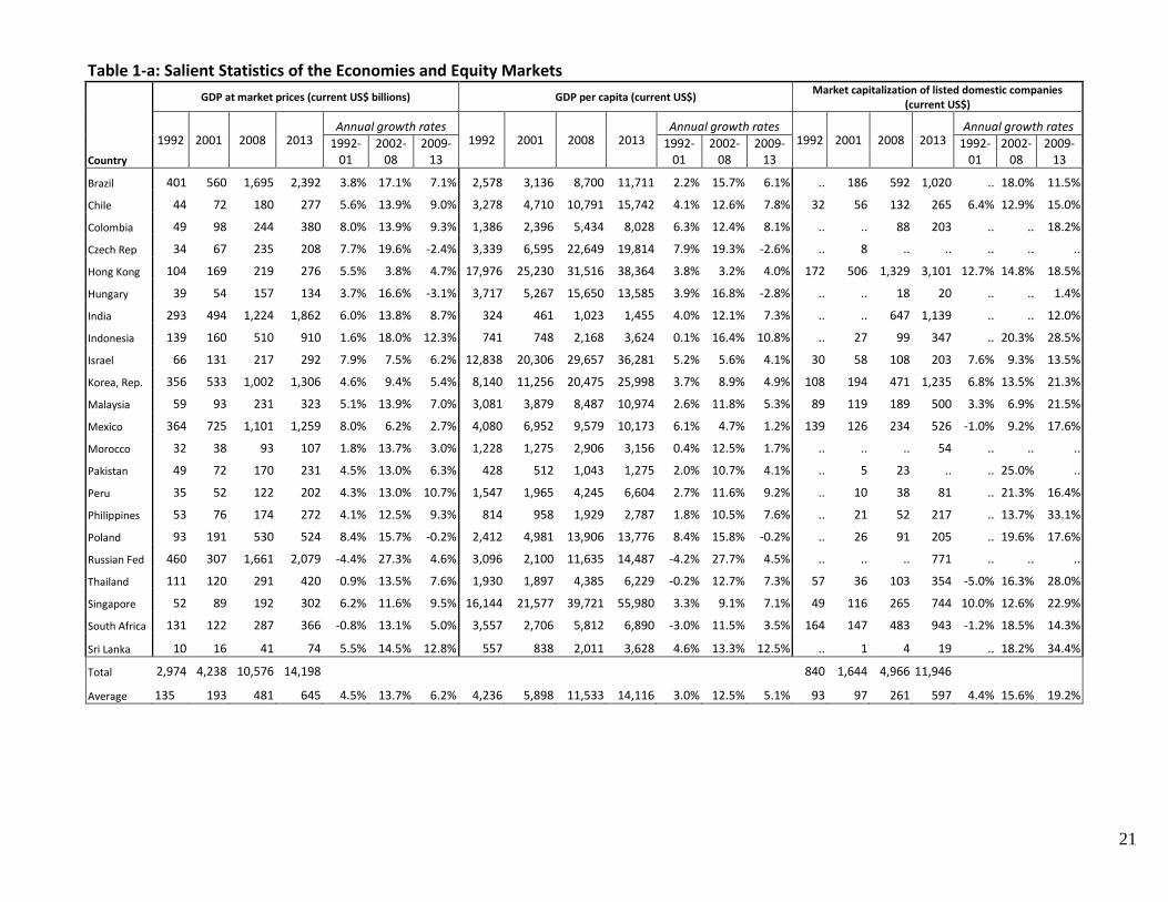
developing countries in the majority. Tables 1a and 1b portray salient features of these economies

for the selected years 1993, 2001, 2008 and 2013, to capture the development of the economies

and the key indicators of financialization over the study period.

As Table 1a shows, the sample includes large economies in terms of GDP (e.g., India,

Mexico and Brazil) as well as smaller economies (e.g., Sri Lanka, and Morocco), and countries at

various stages of development, in terms of Gross National Income per capita (e.g., Bangladesh

and Singapore). Majority of the sample falls in the emerging or frontier markets category, though

Hong Kong, Singapore and South Korea are classified as developed markets. The countries vary

widely across regions and economic systems. There is also a considerable disparity in their

growth rate over the period, and economic structure. Since the beginning of the study period

(1993) statistics, one can see that overall the economies have experienced substantial economic

growth. The countries recorded an average rate of GDP growth of 4.5% during the 1993-2001

period which accelerated to 13.7% p.a. during the following seven years (2001-08), but dropped

to 6.2% p.a. following the global financial crisis starting 2008.

An important development has been the increasing role of the financial markets in the

countries’ economies. The total equity market capitalization for the countries in the sample

increased from US$ 840 billion to US$ 1,644 billion in 2001, registering an annual growth rate of

4.4%. The total capitalization, however, increased three times in the following seven years to US$

4,966 billion, at an annual rate of 15.6%. Following the Global Financial Crisis, however, the

total market capitalization further increased by about 2½ times to US$ 11,946 billion in the next

five years (at annual compound growth rate of 19.2%).

5

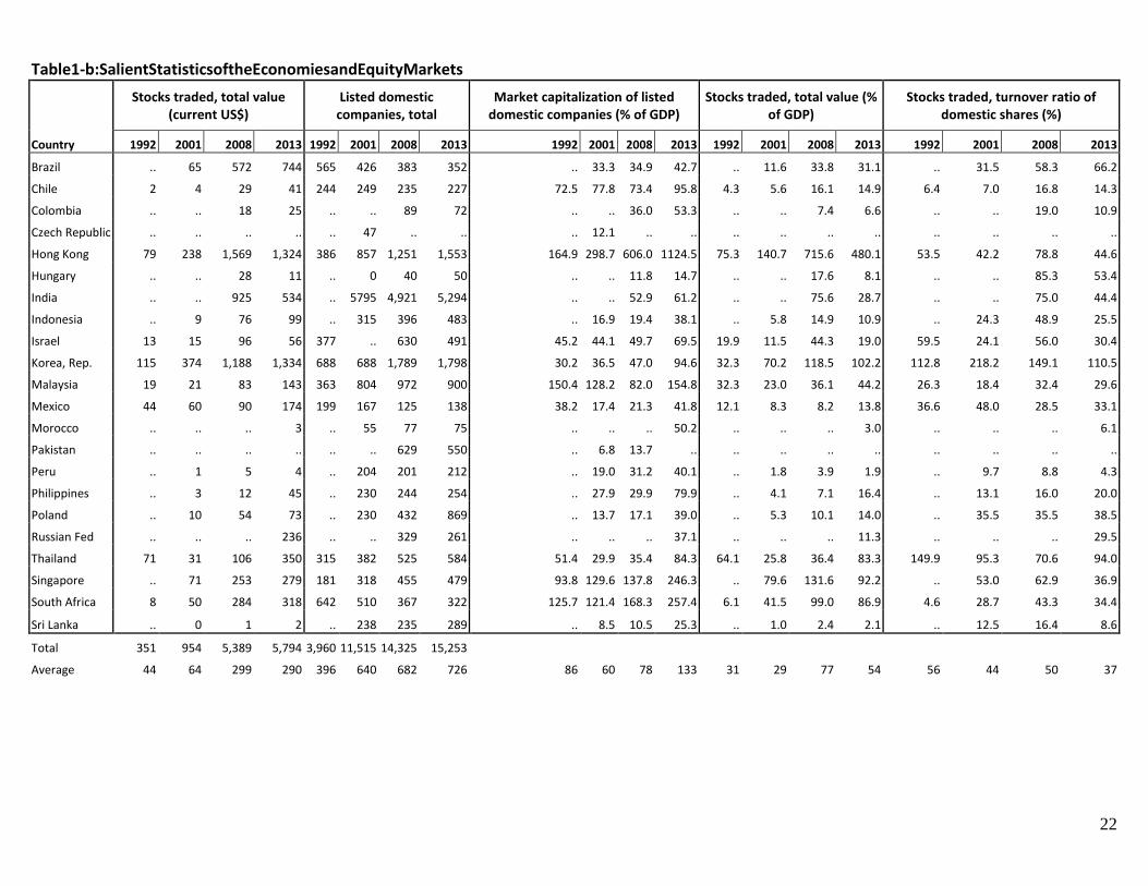
The average market capitalization as a percentage of the GDP, which had remained in the

range of 86%-78% up to 2008, increased to 133% by the end of 2013 as can be seen in Table 1b.

The table also provides salient statistics for the stock markets in the sample countries for the

selected years for comparison. The table shows stocks traded (total value in current US$), number

of listed domestic companies, total market capitalization of listed domestic companies (% of

GDP), the total value stocks traded (% of GDP), and the turnover ratio of domestic shares traded.

All statistics show robust markets growth and a high level of trading activity indicating

financialization of the economies. However, there has been substantial disparity within the

sample as to both the market growth as well as market activity.

Over the study period the emerging markets have implemented important capital market

reforms, which have included stock market liberalization, improvements in securities clearance

and settlements mechanisms, and the development of regulatory and supervisory frameworks.

The privatization of state-owned enterprises and the development of financial institutions such as

privately managed pension funds, have further spurred the growth in the capital markets. These

capital markets reforms taken in the early 1990’s were part of the overall financial liberalization

efforts, and included liberalizing interest rates, shifting to indirect instruments of monetary

control, dismantling directed credit, and opening the capital account to foreign flows. In the mid

1990’s the emphasis of reforms was on strengthening financial sector infrastructure and

individual institutions. During this period, the scope of the financial sector reforms expanded to

include strengthening the legal framework for the banking systems, and developing regulatory

framework and governance environment for corporate sector and securities markets. At the same

time strengthening the enforcement of insider trading laws, accounting and auditing standards

were emphasized.

In the wake of the Asian financial crisis (1997-98) the financial sector reforms assumed a

new urgency. The crisis demonstrated that the corporate and financial sectors are interlinked and

the adverse events in one can have consequences for the other. The reforms that followed these

crises focused on the need for greater transparency and accountability, and ownership structure.

The developing countries implemented a number of fundamental reforms for improving

transparency and accountability. These included steps for improving disclosure of

macroeconomic information, disclosure requirements for securities markets participants, and

investor education. The countries saw establishment of rating agencies and credit bureaus and

adoption of international accounting and auditing standards.

6

In the 2000’s the deepening and broadening of the financial markets continued. The

countries have seen expansion and maturation of financial institutions such as mutual funds,

pension funds, and insurance companies, many of which were established in the mid-1990s. The

availability of financial instruments has been broadened with the establishment and expansion of

derivative markets, commodities exchanges, and electronic trading platforms. In a number of

these markets a variety of derivative instruments have been made available for hedging risk,

although as the financial crisis of late 2008 warns us, sometimes the availability of some of these

instruments may reduce the broader resilience of the financial system, even as they increase the

ability of agents to manage risk in the short run.

The Global Financial Crisis of 2008 (GFC) has had far reaching and extreme effects on

the financial markets crosswise over nations. Stock market volatility expanded numerous folds

throughout the time of crisis, all economic sectors encountering extreme returns. Exceptional

expansive swings in the stock prices were seen with a recurrence which had never been

experienced previously. This brings up a fascinating issue of whether the financial markets over

the globe experienced speculative bubbles leading to the financial crisis, and has the experience

of financial crisis led to a toning downing of the animal spirits associated with such bubbles. The

Global Financial crisis period provides us with an opportunity to investigate the incidence of

speculative behavior of the stock markets over time as financialization took hold. In the past,

financial and monetary crisis, such as the Asian Flu, the Tequila Crisis or the Russian Virus, have

tended to be preceded by periods of speculations. These crashes have been infectious across

countries and have prompted gigantic bailouts by the global organizations to stem contagion.

III. Theoretical Problems of Speculative Bubbles

The conventional theoretical approach to speculative bubbles in the financial economics

literature has been to identify it as a price of an asset staying away from the fundamental value of

the asset for some extended period of time. While it is easier to theoretically hypothesize the

existence of stationary bubbles that can easily arise in overlapping generations models, even with

homogeneous agents possessing rational expectations (Tirole, 1985), such as has been argued is

the case for fiat monies with positive values (whose fundamental values are presumably zero, or

barely above it, “the value of the paper the money is printed on”), such bubbles are essentially

impossible to identify in practice. It is the exploding bubbles, or at least the sharply increasing

ones, that we have any hope of empirically observing, even if the theory behind how they can

arise is less general than that for the stationary bubbles.

7

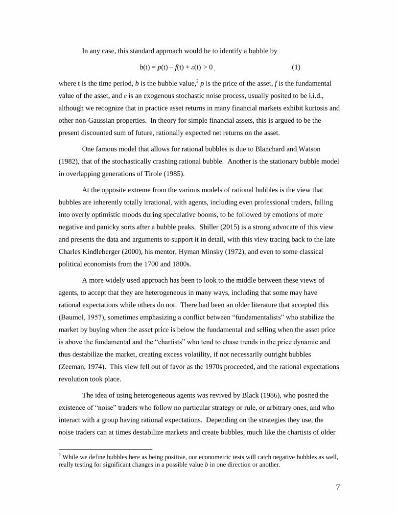
In any case, this standard approach would be to identify a bubble by

b(t) = p(t) – f(t) + ε(t) > 0 , (1)

where t is the time period, b is the bubble value,2 p is the price of the asset, f is the fundamental

value of the asset, and ε is an exogenous stochastic noise process, usually posited to be i.i.d.,

although we recognize that in practice asset returns in many financial markets exhibit kurtosis and

other non-Gaussian properties. In theory for simple financial assets, this is argued to be the

present discounted sum of future, rationally expected net returns on the asset.

One famous model that allows for rational bubbles is due to Blanchard and Watson

(1982), that of the stochastically crashing rational bubble. Another is the stationary bubble model

in overlapping generations of Tirole (1985).

At the opposite extreme from the various models of rational bubbles is the view that

bubbles are inherently totally irrational, with agents, including even professional traders, falling

into overly optimistic moods during speculative booms, to be followed by emotions of more

negative and panicky sorts after a bubble peaks. Shiller (2015) is a strong advocate of this view

and presents the data and arguments to support it in detail, with this view tracing back to the late

Charles Kindleberger (2000), his mentor, Hyman Minsky (1972), and even to some classical

political economists from the 1700 and 1800s.

A more widely used approach has been to look to the middle between these views of

agents, to accept that they are heterogeneous in many ways, including that some may have

rational expectations while others do not. There had been an older literature that accepted this

(Baumol, 1957), sometimes emphasizing a conflict between “fundamentalists” who stabilize the

market by buying when the asset price is below the fundamental and selling when the asset price

is above the fundamental and the “chartists” who tend to chase trends in the price dynamic and

thus destabilize the market, creating excess volatility, if not necessarily outright bubbles

(Zeeman, 1974). This view fell out of favor as the 1970s proceeded, and the rational expectations

revolution took place.

The idea of using heterogeneous agents was revived by Black (1986), who posited the

existence of “noise” traders who follow no particular strategy or rule, or arbitrary ones, and who

interact with a group having rational expectations. Depending on the strategies they use, the

noise traders can at times destabilize markets and create bubbles, much like the chartists of older

2 While we define bubbles here as being positive, our econometric tests will catch negative bubbles as well,

really testing for significant changes in a possible value b in one direction or another.

8

models. Day and Huang (1990) followed this with a model that added market makers to this

setup and showed the possibility of a wide variety of dynamic paths for asset prices, including

dynamically chaotic ones. Impetus for such an approach increased after DeLong et al (1991)

demonstrated that such noise traders could not only survive but even thrive in markets that also

contained traders with rational expectations, thus overturning an old argument that such traders

would lose money and be driven from the markets.

Eventually this general approach evolved to allow for wider varieties of heterogeneous

interacting agents, who could learn and change strategies over time, with Föllmer et al (2005)

providing a general theoretical perspective on such approaches and Hommes (2006) and LeBaron

(2006) provide broad summaries and reviews of them. We shall look briefly at one such model

that can produce a wide variety of dynamic paths, due to Bischi et al (2006), which in turn draws

on Chiarella et al (2003), a discrete choice model of agents whose strategies evolve over time in

response to their performance. This approach was initiated by Brock and Hommes (1997).

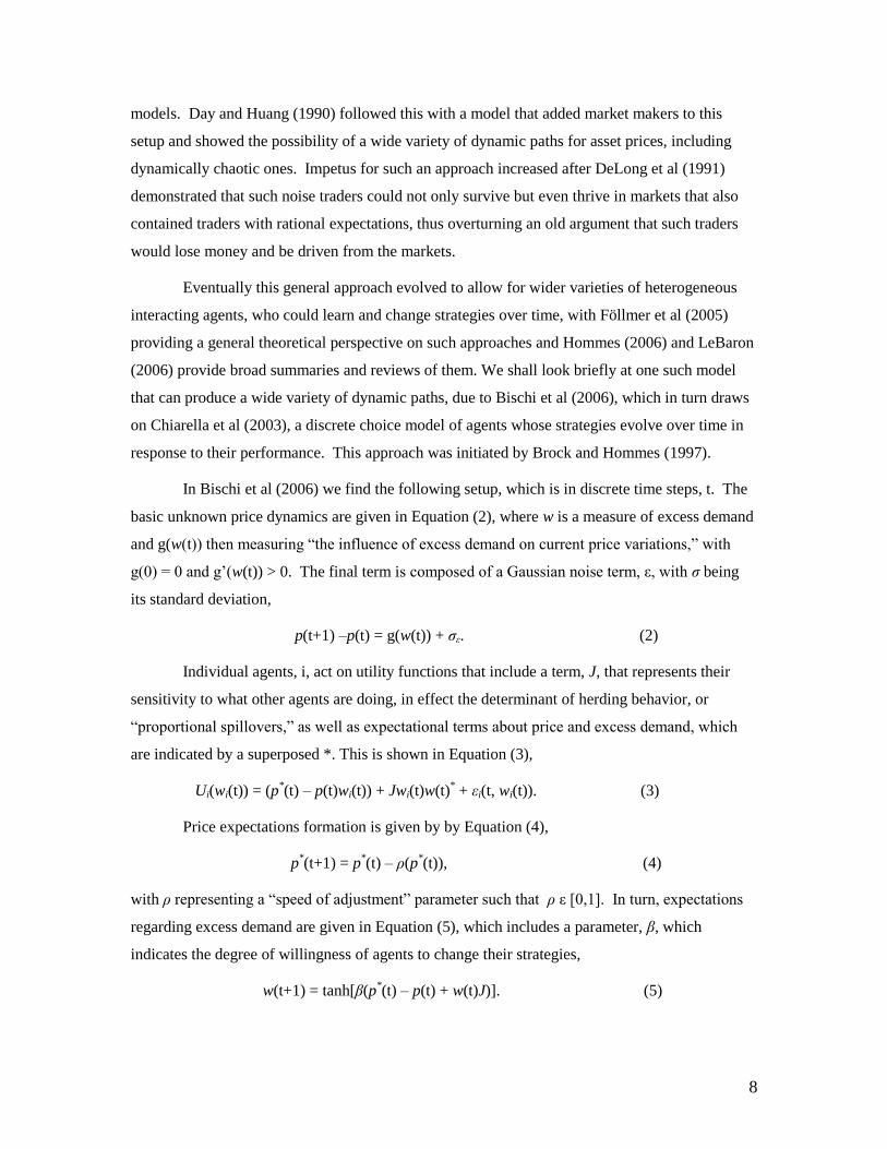
In Bischi et al (2006) we find the following setup, which is in discrete time steps, t. The

basic unknown price dynamics are given in Equation (2), where w is a measure of excess demand

and g(w(t)) then measuring “the influence of excess demand on current price variations,” with

g(0) = 0 and g’(w(t)) > 0. The final term is composed of a Gaussian noise term, ε, with σ being

its standard deviation,

p(t+1) –p(t) = g(w(t)) + σε. (2)

Individual agents, i, act on utility functions that include a term, J, that represents their

sensitivity to what other agents are doing, in effect the determinant of herding behavior, or

“proportional spillovers,” as well as expectational terms about price and excess demand, which

are indicated by a superposed *. This is shown in Equation (3),

Ui(wi(t)) = (p*(t) – p(t)wi(t)) + Jwi(t)w(t)

* + εi(t, wi(t)). (3)

Price expectations formation is given by by Equation (4),

p*(t+1) = p

*(t) – ρ(p

*(t)), (4)

with ρ representing a “speed of adjustment” parameter such that ρ ε [0,1]. In turn, expectations

regarding excess demand are given in Equation (5), which includes a parameter, β, which

indicates the degree of willingness of agents to change their strategies,

w(t+1) = tanh[β(p*(t) – p(t) + w(t)J)]. (5)

9

It turns out that the nature of the dynamics are ultimately shaped by the respective values of β and

J, with generally speaking more volatile and complex dynamics arising when these parameters

are of higher values above certain critical levels.3 Simulations of this model are able to replicate

patterns that we see regularly in financial markets, with periods of relatively stable behavior

alternating with periods of heightened volatility, driven by oscillations in which different

strategies are dominant among the agents at different times.

We close this section by noting that this is simply a representative model, which we are

not attempting to estimate per se in what follows (the relevant parameters being hard to estimate

from actual market data), which uses a more generic time-series approach, although we do model

the fundamental with a vector auto-regression (Engle, 1982) that uses certain macroeconomic

variables.

IV. Data and Methodology:

This paper uses methods from Ahmed et al (2006, 2010), which in turn combined

methods used in Ahmed et al (1996) and in Ahmed et al (1997)4, to test for the absence of

excessively rapid movements of price movements in daily stock market indices in 23 market

economies from 1993 to 2015 as well as to test for absence of nonlinearities beyond ARCH

effects. Failure to reject such absences is seen as possible evidence for the presence of nonlinear

speculative bubbles in such markets. This would confirm a widely held perception that many

such markets have exhibited such bubbles, possibly even more so than the markets of either more

fully developed or less developed economies (although we do not test for either of these last

hypotheses). While such bubbles are seen as destabilizing and disruptive to these economies in

many ways, they are also seen as often accompanying waves of real investment that are crucial to

the development process, which means that a nation may or may not wish to reduce or eliminate

such bubbles.

Our method is to estimate time-series for likely fundamentals of the daily stock market

indices using vector auto-regressions (VAR) of the stock market index returns with a leading

country interest rate, the country’s foreign exchange rate, a world interest rate, and average world

3 This approach draws ultimately from statistical physics of interacting particle systems, with β being

related to temperature and J related to the strength of interactions between the particles. These parameters

are difficult to estimate from actual data. An extension of this approach that brings in the Minsky approach

is due to Gallegati et al (2011), with a further discussion of related policy issues by Rosser et al (2012). 4 Ahmed et al (1996) studied such phenomena in the Pakistani stock market while Ahmed et al (1997)

looked at such bubbles in closed-end country funds. In addition, Ahmed et al (2006) focused on the

Chinese stock markets of the 1990s, with Ahmed et al (2010) applying this to a set of emerging market

stock markets prior to the Great Recession.

10

stock market returns. We then subject the residuals of these hypothesized fundamental series for

each country to two separate tests for excessively rapid movements away from the fundamental

(or more precisely test for the absence of such movements). The first test is the regime switching

test due to Hamilton (1989) and the second is the rescaled range analysis (RRA) due originally to

Hurst (1951). We then estimate and remove ARCH effects for each series and test for the

absence of additional nonlinearities using the BDS test (Brock et al, 1997), although we do not

seek to determine more precisely the forms of these nonlinearities, which presumably vary from

country to country. For all countries, at the 1% level of significance we fail to reject the absence

of such bubbles, the presence of further nonlinearities beyond ARCH, using the BDS test.

A number of efforts have been made recently by others to study such dynamics in one

form or another in such markets, with much of the focus being on the especially volatile stock

markets of China. Ahmed et al (2006) studied this issue for 1999 data, and were unable to reject

the presence of nonlinear bubbles. Jiang et al (2010) found long memory in the Chinese and

Japanese stock markets using detrended fluctuation analysis, indicative of rejection of the

efficient market hypothesis. Thiele (2014) finds persistence and fractal patterns in the Chinese

market and suggests that regulations may have aggravated the potential for bubbles5. Sarkar and

Mukhopadhyay (2005) found a variety of anomalies and nonlinear dependence in the Indian stock

markets, with Hiremath (2014, chaps. 5-6) providing more detailed discussion of the Indian case.

Ciner and Karagozoglu (2008) have found such nonlinear bubbles to arise from asymmetric

information in the Turkish stock market.

At this point we warn of an important caveat to this analysis. This is the ubiquitous

problem of the misspecified fundamental, first identified by Flood and Garber (1980). The

problem is that to identify a bubble one must be certain that one has correctly identified the

fundamental series from which it is seen to be deviating from. What one sees as a bubble might

actually be the fundamental if it reflects rational expectations of a substantial increase in the

future of the fundamental that simply turns out not to be realized. Only a few assets can avoid

this problem to some extent, with closed-end funds whose fundamentals are the values of the

assets constituting them (with some adjustment for tax or liquidity matters) being such an

example (Ahmed et al, 1997). Thus, while our approach to estimate the fundamental series for

these stock markets has been used by others (Canova and Ito, 1991), we cannot guarantee that we

have determined proper fundamentals for these stock markets. So, even though the evidence we

5 These dynamics have also happened despite China maintaining capital controls in its foreign exchange

markets, something recommended even by Bhagwati (2007) who supports free trade and increased

economic globalization in general.

11

present is quite strong for almost all of these markets, it cannot be viewed as conclusive.

However, even if we cannot say for certain that we have identified speculative bubbles, the

econometric techniques we use can be said to identify sharp movements that can be identified as

at least constituting “high volatility.”

V. Empirical Tests of Speculative Bubbles

We examine daily returns behavior in the sample countries over periods 1993-2013. For

each country, we use daily values of the market’s major index, and compute stock index ‘returns’

as the first log differences; RI,t = ln(Indext) - ln(Indext-1). These index returns were then used in a

Vector Autoregressive (VAR) model with those of daily interest rates, daily exchange rates and

World Stock index returns as a measure of the presumptive fundamental. Two alternative series

of interest rates were used for some countries; the first representing short-term rates for 30-days

or less maturity and the second set of interest rate series represented rates on relatively longer-

term one year maturity instruments.6 These interest rates were proxied, depending on the

availability of data for each country, by various rates series, including CD rate, inter-bank

overnight rate, T-Bill auction yields, bank base rates, and bank loan rates. To capture the impact

and the linkages of the developed markets on the fundamental of the sample countries we also

included MSCI World index in the VAR model. The MSCI World index, maintained by Morgan

Stanley Capital International, is considered a stock market index of ‘world portfolio’ and includes

a collection of stocks of all the 23 developed markets in the world, as defined by MSCI, for which

returns are calculated as for the local indices. The data on the stock market indices, interest rates

and exchange rates was obtained from the Datastream International, Ltd. database.

Residuals from the resulting VARs are used for the bubble tests, with ARCH effects

removed later for the BDS nonlinearity tests. We then carry out three types of tests: (i) the regime

switching tests, (ii) the rescaled range tests, and the (iii) nonlinearity tests.

i) Regime Switching Tests

Hamilton (1989) introduced an approach to regime switching tests that can be used to test for

trends in time series and switches, with a more complete analysis in Hamilton, (1994, Chap. 22).

We use this approach as our main test for the null of no bubbles on the residual series derived

above which is given by

t = nt + zt (6)

6 Arguably we should include a measure of monetary policy. However, such policies do not change daily

except as manifested in daily changes of interest rates.

12

where

nt = 1 + 2st (7)

and

zt - zt-1 = 1(zt-1 - zt-2) +…+r (zt-r - zt-r-1) + t (8)

with s = 1 being a positive trend, s = 0 being a negative trend, and I 0 indicating the possible

existence of a trend element beyond the VAR process. Furthermore, let

Prob [st = 1 st-1 = 1] = p, Prob [st = 0 st-1 = 1] = 1 - p (9)

Prob [st = 0 st-1 = 0] = q, Prob [st = 1 st-1 = 0] = 1 - q. (10)

Following Engel and Hamilton (1990) a "no bubbles" test proposes a null hypothesis of no

trends given by p = 1 - q. This is tested by with a Wald test statistic given by

[p - (1 - q)]/[var(p) + var(1 - q) + covar(p, 1 - q)]. (11)

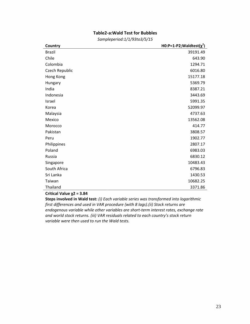
Results: The regime switching tests results are reported in table 2a which shows the χ2

values for the Wald Test for bubbles (H0: p = 1- q) as explained above. The critical value for

rejecting the null of no trends is 2 = 3.8. Clearly, the null is strongly rejected in all countries for

the full sample period from 1/1/1993 to 3/5/15. In order to examine the incidence of speculative

bubbles over time we sub-divide the full sample into four sub-periods as follows:

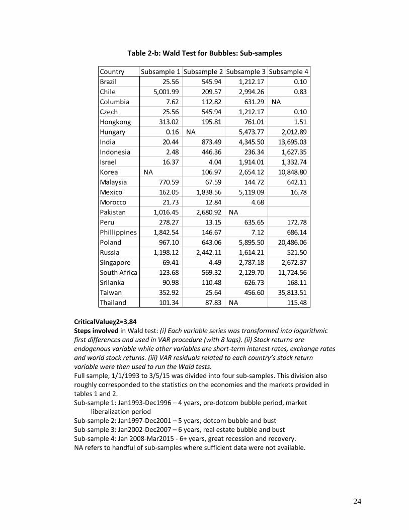
1. Sub-sample 1: Jan 1993 - Dec 1996 - 4 years, market liberalization, pre-dotcom bubble.

2. Sub-sample 2: Jan 1997 - Dec 2001 - 5 years, dotcom bubble and bust.

3. Sub-sample 3: Jan 2002 - Dec 2007 - 6 years, real estate bubble and bust.

4. Sub-sample 4: Jan 2008 - Mar 2015 - 6+ years, great recession and recovery.

The division also roughly corresponded to the statistics on the economies and the markets

provided in tables 1 and 2.

Table 2b contains the results of the regime switching tests for the four subsamples. The null

hypothesis of no trends is strongly rejected in the preponderance of the tests (countries and the

sub-samples), the test statistics exceeding the critical value of 2 = 3.8. However, the null is not

rejected for the sub-sample 4 for Brazil, Chile, Czech Republic and Hong Kong, and for sub-

period 1 for Hungary and Indonesia. Also, for some sub-periods the statistic could not be

computed due to insufficient data. Although, we did not conduct a formal statistical test for the

difference in the incidence of bubbles across the four subsamples, the magnitude of the test

statistic 2 may be used to make an inference as to whether a market was more or less bubbly

13

from one period to another. When we compare the values of the Wald test statistics from one

period to the next we find that there is quite a variation in the 2 value from one period to the

other; countries depict a varied pattern across time. In the case of a few countries (India and

South Africa) the Wald statistic shows an increase between each sub-period, i.e., sub-periods 2 vs

1, 3 vs 2 and 4 vs 3. We find that comparing sub-period 2 to sub-period 1 (the market

liberalization period), the value of the test statistic increased in about half the sample (10 out of

21), but decreased in the other half (11/21). However, the markets depict a marked increase in the

speculative behavior (as indicated by the magnitude of the 2 statistic) when we compare sub-

period 3 to 2 (the statistic is higher in 16 out of 20 countries), and sub-period 3 to 1 (the statistic

is higher in 17 out of 21 countries). Comparing the sub-period 4 (the post Global Crisis period) to

sub-period 3 (the pre-Global Crisis period) we find that the magnitude of the statistic decreased in

majority of the markets (11 out of 19 countries), in particular we see no evidence of the presence

of speculative tends in four countries, as noted above. Nevertheless, the value of the statistic is

higher for half the sample. The post-Global Crisis period seems to have attenuated the incidence

of speculative bubbles to some extent. Yet, the overall picture is that there seems to be a secular

trend towards increasing tendency for the market to exhibit speculative behavior.

ii) Hurst Persistence Tests

Hurst (1951) developed a test to study persistence of Nile River annual flows, which was first

applied to economic data by Mandelbrot (1972). For a series xt with n observations, mean of x*m

and a max and a min value, the range R(n) is:

R(n) = [max 1kn ∑ (x𝑗 − x∗)𝑘𝑗=1 - min 1kn ∑ (x𝑗 − x∗)𝑘

𝑗=1 ] (12)

The scale factor, S(n, q) is the square root of a consistent estimator for spectral density at

frequency zero, with q < n,

S(n, q)2 = g0 + 2 ∑ 𝑤𝑗

𝑞𝑗=1 (q)gj, wj(q) = 1 - [j/(q-1)], (13)

with g’s autocovariances and w’s weights based on the truncation parameter, q, which is a period

of short-term dependence.7 The classical Hurst case has q = 0, which reduces the scaling factor to

a simple standard deviation.

Feller (1951) showed that if xt is a Gaussian i.i.d. series then

7 Lo (1991) has criticized the use of the classical Hurst coefficient for studying long-term persistence in

stock markets precisely because of this presence of short-term dependence for which he proposes a method

to avoid such dependence. However, this is not a problem for us because it is precisely short-term

dependence that we are interested in detecting.

14

R(n)/S(n) nH, (14)

H = ½ implies integer integro-differentiation and thus standard Brownian motion, the "random

walk." H is the Hurst coefficient, which can vary from zero to one with a value of 1/2 implying

no persistence in a process, a value significantly less than 1/2 implying "anti-persistence" and a

value significantly greater than 1/2 implying positive persistence. The significance test involves

breaking the sample into sub-samples (namely, pre-bubble, during-bubble and post-bubble

period) and then estimating a Chow test on the null that the sub-periods possess identical slopes.

This technique is also called rescaled range analysis. Sub-samples are determined on visual

examination of the entire stock returns series. While we did not use a formal technique to seek

structural breaks, we note that the bias for not doing so is to weaken the results as such techniques

work to maximize the differences between the various sub-samples.

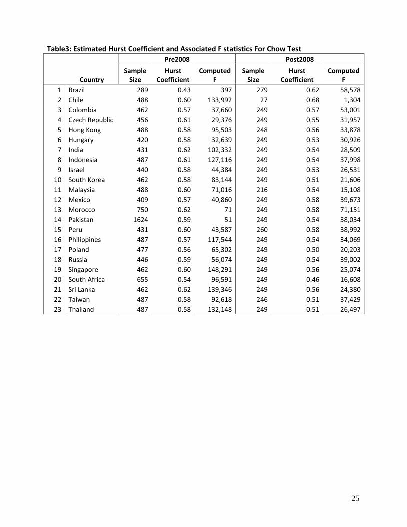
Results: The Hurst persistent test is conducted for two sample, pre- and Global Financial

Crisis (2007) periods; first period is from January 2002 to December 2007, and the second is

from January 2008 to March 2015. Table 3 presents the results of this test.

For each country H (Hurst) coefficient is estimated and as can be seen the value of the

estimated value of the coefficient is above 0.50 for all countries in both sub-periods, except for

one Brazil, (H=0.46) for the pre-GFC period and for Poland (H=0.50) and South Africa (H=0.46)

for the post-GFC period. The median Hurst Coefficient is 0.58 for the first and 0.54 for the

second period. The F values reported in the table are for the Chow tests which involves breaking

the sample into sub-samples (namely, pre-bubble, during-bubble and post-bubble period) and

then testing the null that the sub-periods data possess identical slopes, explained above.

As the table shows the computed F-values for all of the countries are substantially above

the critical value showing a significant rejection of the null hypothesis that the coefficient is equal

to 0.50 (thus indicating no persistence). Results are reported for a test of a model with the

intercept suppressed.

iii) Nonlinearity Tests

We test for nonlinearity of the VAR residual series in two stages. The first is to remove

ARCH effects. Engle (1982) showed that the nonlinear variance dependence measure of

autoregressive conditional heteroskedasticity (ARCH) as

xt = tt (15)

15

t2 = 0 + ∑ 𝑖

𝑛𝑖=0 xI-i

2 (16)

with i.i.d. and the I's different lags. We use a three period lag and, as expected, found

significant ARCH effects in all series, available on request from the authors.8

The second stage involves removing variability attributable to the estimated ARCH effects

from the VAR residual series for both models. The remaining residual series is run through the

BDS test due to Brock, Dechert, LeBaron, and Scheinkman (1997). This statistic tests for

generalized nonlinear structure but does not test for any specific form such as alternative ARCH

forms or chaos.

The correlation integral for a data series xt, t = 1,…,T, results from forming m-histories such

that x = [xt, xt+1, …, xt+m+1] for any embedding dimension m. It is

cmT() = ∑ I𝑡<𝑠 (xtm, xs

m)[2/Tm(Tm-1)] (17)

with a tolerance distance of , conventionally measured by the standard deviation divided by the

spread of the data, I(xtm, xs

m) is an indicator function equaling 1 if │I(xt

m, xs

m)│< and equaling

zero otherwise, and Tm = T - (m - 1).

The BDS statistic comes from the correlation integral as

BDS (m, ) = T1/2

{cm() - [c1()]m}/bm (18)

where bm is the standard deviation of the BDS statistic dependent on the embedding dimension m.

The null hypothesis is that the series is i.i.d., meaning that for a given and an m > 1, cm() -

[c1()]m equals zero. Thus, sufficiently large values of the BDS statistic indicate nonlinear

structure in the remaining series. This test is subject to severe small sample bias with a cutoff of

500 observations sufficient to overcome this, a minimum both of our daily series easily achieve.

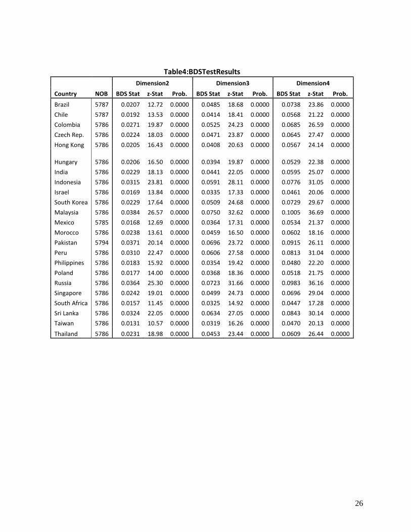
Results: Table 4 presents the results of this test for embedding dimensions, m = 2 to 4 (m

= 3 is conventional). The critical value for rejecting the null of i.i.d. is approximately 6. Based

on the estimated BDS statistics null is rejected for all cases except one case (Israel sample 2).

Thus, there appears to be remaining nonlinearity beyond basic ARCH in the VAR residual series.

Of course, just as our earlier tests are subject to the validity of our original VAR

specifications, likewise so is this test. We emphasize that the nature of the remaining nonlinearity

remains unknown. It is likely that different models of nonlinearity will work better for each

8 We have tried different lags and also alternative simple GARCH tests, with no great differences. Of

course there is a large set of alternative GARCH-related measures.

16

country than others, but finding which is best for each is a task beyond the scope of this paper.

However, we note that without knowing the nature of the complex dynamics, it will be very hard

for any particular government to intervene with confidence in its financial markets to achieve a

given result. Unexpected things may well happen.

VI. Discussion and Conclusions

We have shown that for a set of 23 markets around the world, there is strong evidence of

the presence of nonlinear speculative bubbles in their stock markets during the period of 1993-

2015. Regime switching tests rejected the null hypothesis of no bubbles for all countries. The

rescaled range tests also find rejection for the same null hypothesis for all countries. Moreover,

the test for nonlinearity beyond ARCH effects using the BDS statistic rejected the null of no such

nonlinearity. For most of these tests the rejection of the null was overwhelming.

We recognize that we may not have accurately specified the fundamentals of the stock

market. Yet, at a minimum our findings show that the stock markets in just about all of the

countries in our sample have exhibited considerable volatility, persistence and non-linearities

during the study period; it is in effect what the empirical tests used here can claim to show. Even

if the existence of true speculative bubbles is not proved, the markets in these countries have

clearly experienced large and sudden fluctuations. Many of these fluctuations are likely to be due

to speculative bubbles. This is further supported by the fact that these fluctuations have tended to

be far greater than attributable to the underlying fluctuations of macroeconomic variables as

shown the macro-economic data provided in tables 1 and 2. Additionally, the reported and

anecdotal evidence out of most of these countries suggests that market participants believe that

they have frequently observed such bubbles. This long term trend appears to have been somewhat

moderated in the post-Global Crisis period, which may have led to attenuation of the speculative

proclivities to some extent. Yet, the overall picture is that there seems to be a secular trend

towards increasing tendency for the market to exhibit speculative behavior. We have discussed

how the period under study has been characterized by the financialization phenomenon. We have

not conducted a robust statistical test of the association of the observation of increased incidence

of bubbles and the financialization of the economies. Nevertheless, our findings provide a prima

facie evidence of the association between the two.

The apparently linkage of the prevalence of bubbles and financialization certainly raises

public policy challenges for the governments and the financial regulators. Participants in the

financial markets do not like excessive volatility, and certainly market crashes can have

17

devastating consequences for the economy. Indeed, macro-economic policies in most countries

seek to stabilize financial markets and to deflate asset bubble. However, it may well be that such

bubbles are an inevitable part of the development of financial systems particularly in the

emerging market economies, but the markets in more developed and established economies are

not immune to such bouts either.

The conundrum for policymakers is that while bubbles can distort economic allocation

and activity, they may also be an inevitable in process of the development. Theoretical models of

smooth growth do not reflect the reality of the development experience. In reality development

involves spurts of growth associated with investment surges in particular sectors. Such

investment surges may well require outbreaks of excessive enthusiasm, the “animal spirits” of

Keynes, in order to bring forth the investment surge. Such outbreaks of enthusiasm will readily

show up in stock markets as outbreaks of enthusiasm regarding the stock in such a sector, with

the likelihood of speculative bubbles in those stocks emerging. As long as financial markets exist

it may be impossible to avoid speculative bubbles. Increasing experimental evidence shows the

tendency to bubbles as deeply rooted in the human psyche, occurring even when agents are fully

informed about the situations that they are in (Porter and Smith, 1994).

The price of slowing the growth of the financial sector to ward off ill-effects of

financialization and possibly avoiding bubbles may be slower economic growth. Certainly it is

possible for countries to increase regulation of the financial sector or use either direct capital

controls or indirect monetary policy tools such as raising interest rates or margin requirements.

However, the demand for modern and innovative financial products from market participants will

likely continue to be strong, who may bring political pressure to bear to resist such efforts.

Broader contractionary monetary policy can simply slow growth and bring on a recession, and

raise unemployment; governments, therefore, face hard choices. Also, the presence of

nonlinearities suggests that these bubbles are complex, so that predicting the impacts of trying to

manage them through any policies may be difficult, certainly without a better understanding of

the particular dynamics of a particular country’s financial markets.

The financial crises of 2007 caution us that the financial innovations and availability of

low cost financing may also bring risks and dangers, including the risk of spawning of bubbles.

However, the experience of this crisis also suggests that these problems are broader and may

affect any economy whose financial markets are connected with those of the rest of the world.

Again, bubbles and crashes may be inevitable, with the forward march of globalization and the

18

expansion of financial instruments in developing financial markets simply making this

inevitability all that more unavoidable. It may be that the best that the governments can do is to

ensure that the victims of the crashes are assisted in such ways as can be arranged and managed

through social safety nets, without harming the broader functioning of their economic systems

and development strategies.

19

References

Ahmed, E., Koppl, R., Rosser, J.B., Jr., and White, M.V. 1997. Complex bubble persistence in

closed-end country funds. Journal of Economic Behavior and Organization 32, 19-37.

Ahmed, E., Li, H., Rosser, J.B., Jr. Nonlinear bubbles in Chinese stock markets in the 1990s.

Eastern Economic Journal 32, 1-18.

Ahmed, E., Rosser, J.B., Jr., and Uppal, J.Y. 1996. Asset speculative bubbles in emerging

markets: The case of Pakistan. Pakistan Economic and Social Review 34, 97-118.

Ahmed, E., Rosser, J.B., Jr., and Uppal, J.Y. 2010. Emerging markets and stock market bubbles:

Nonlinear speculation? Emerging Markets, Finance, and Trade 46, 73-91.

Aalbers, M. B., 2015. The potential for financialization, Dialogues in Human Geography, 5(2),

214–219.

Aalbers, M. B., van Loon, J., and Fernandez, R., 2015. The financialization of a social housing

provider, Paper presented at the RC21 International Conference on “The Ideal City:

between myth and reality. Representations, policies, contradictions and challenges for

tomorrow's urban life” Urbino. http://www.rc21.org/en/conferences/urbino2015/

Aalbers, M. B. 2008. The Financialization of Home and the Mortgage Market Crisis. Competition

& Change, 12(2), 148-166.

Baumol. W.J. 1957. Speculation, profitability, and instability. Review of Economics and Statistics

34, 263-271.

J. Bhagwati. 2007. In Defense of Globalizaton, with a New Afterword. New York: Oxford

University Press.

Bischi, G.-I., Gallegati, M., Gardini, L., Leombrini, R., and Palestrini, A. 2006. Herd behavior

and non-fundamental asset price fluctuations in financial markets. Macroeconomic

Dynamics 10, 502-528.

Black, F. 1986. Noise. Journal of Finance 41, 529-542.

Blanchard, O. and Watson, M.W. 1982. Bubbles, rational expectations, and financial markets. In

P. Wachtel, ed., Crises in the Economic and Financial Structure. Lexington: Lexington

Books,295-315.

Brock, W.A., Dechert,W.D., Scheinkman, J.A., and LeBaron, B. A test for independence based

on the correlation dimension. Econometric Reviews 15, 197-235.

Brock, W.A. and Hommes, C. 1997. A rational route to randomness. Econometrica 65, 1059-

1095.

Canova, F. and Ito, T. 1991. The time series properties in the risk premium of the yen/dollar

exchange rate. Journal of Applied Econometrics 22, 213-223.

Chiarella, C., Gallegati, M., Leombrini, R., and Palestrini, A. 2003. Asset price dynamics using

heterogeneous interacting agents. Computational Economics 22, 213-223.

Cloke, J. 2010. Capital is dead: Long live ultra-capital. In T. Lagoarde-Segot (Ed.), After the

crisis: Rethinking finance. Nova Science, 1–16.

Cloke, J. 2013. Actor-network capitalism and the evolution of ultra-capital. Working paper,

University of Helsinki.

Ciner, C. and Karagozlu, A.K. 2008. Information asymmetries, speculation and foreign trading

activity: Evidence from an emerging market. International Review of Financial Analysis

17, 664-680.

Day, R.H. and Huang, W. 1990. Bulls, bears, and market sheep. Journal of Economic Behavior

and Organization 14, 299-329.

DeLong, J.B., Shleifer, A., Summers, L.H., and Waldmann, R. 1991. The survival of noise traders

in financial markets. Journal of Business 64, 1-19.

Engel, R. and Hamilton,J.D. 1990. Long swings in the dollar: Are they in the data and do markets

know it? American Economic Review 80, 689-713.

20

Engle, R.F. 1982. Autoregressive conditional heteroscedasticity with estimation of the variance of

United Kingdom inflation. Econometrica 50, 251-276.

Feller, W. 1951. The asymptotic distribution of the range of sums of independent random

variables. Annals of Mathematical Statistics 22, 427-432.

Flood,R.P. and Garber, P.M. 1980. Market fundamentals versus price level bubbles: The first

tests. Journal of Political Economy 88, 745-776.

Föllmer, H., Horst, U., and Kirman, A. 2005. Equilibria in financial markets with heterogeneous

agents: A probabilistic approach. Journal of Mathematical Economics 41, 123-155.

Gallegati, M., Palestrini, A., Rosser, J.B., Jr. 2011. The period of financial distress in speculative

markets: Interacting heterogeneous agents and financial constraints. Macroeconomic

Dynamics 15, 60-79.

Hamilton, J.D. 1989. A new approach to the economic analysis of nonstationary time series and

the business cycle. Econometrica 57, 357-384.

Hamilton, J.D. 1994. Time-Series Analysis. Princeton: Princeton University Press.

Hiremath, G.S. 2014. Indian Stock Market: An Empirical Analysis of Informational Efficiency.

New Delhi, Springer.

Hurst, H.E. 1951. Long term storage capacity of reservoirs. Transactions of the American Society

of Civil Engineers 116, 770-799.

Jiang, Z.-Q., Zhou, W.-X., Sornette, D., Woodard, R., Bastiaensean, and Cauwels, P. 2010.

Bubble diagnosis and prediction of the 2005-2007 and 2008-2009 Chinese stock market

bubbles. Journal of Economic Behavior and Organization 74, 149-161.

Kaminsky, G.L. and Reinhart, C.M. 1999. The twin crises: the causes of banking and balance-of-

payment problems, American Economic Review, 89(3), 473–500.

Kindleberger, C.P. 2000. Manias, Panics, and Crashes, 4th edition. New York: Wiley.

Minsky, H.P. 1972. Financial instability revisited: The economics of disaster. Reappraisal of the

Federal Reserve Discount Mechanism 3, 97-136.

Lo, A.W. 1991. Long memory in stock prices. Econometrica 59, 1279-1313.

Mandelbrot, B.B. 1972. Statistical methodology for nonperiodic cycles: From covariance to R/S

analysis. Annals of Economic and Social Measurement 1, 259-290.

Palley, T. I. 2007. Financialization: What it is and why it matters, Paper presented at a conference

on “Finance-led Capitalism? Macroeconomic Effects of Changes in the Financial

Sector,” the Hans Boeckler Foundation, Berlin, Germany.

Rosser, J.B., Jr., Rosser, M.V., and Gallegati, M. 2012. A Minsky-Kindleberger perspective on

the financial crisis. Journal of Economic Issues 45, 449-458.

Sarkar, N. and Mukhopadhyay. 2005. Testing predictability and nonlinear dependence in the

Indian stock market. Emerging Markets, Finance and Trade 41, 7-44.

Shiller, R.J. 2015. Irrational Exuberance, 3rd

edition. Princeton: Princeton University Press.

Thiele, T.A. 2014. Multiscaling and stock market efficiency in China. Review of Pacific Basin

Financial Markets and Policies 17, doi 1450023.

Tirole, J. 1985. Asset bubbles and overlapping generations. Econometrica 53, 1499-1528.

Vitali, S., Glattfelder, J. B., and Battiston, S. 2011. The network of global corporate control. PLoS

One. 2011; 6(10): e25995. Published online 2011 Oct 26. doi:

10.1371/journal.pone.0025995

Walter, C., 2016. The financial Logos: The framing of financial decision-making by

mathematical modelling, Research in International Business and Finance, 37, 597–604.

Zeeman, E.C. 1974. On the unstable behavior of the stock exchange. Journal of Mathematical

Economcs 1, 39-44.

21

Table 1-a: Salient Statistics of the Economies and Equity Markets

GDP at market prices (current US$ billions) GDP per capita (current US$)

Market capitalization of listed domestic companies (current US$)

1992 2001 2008 2013

Annual growth rates 1992 2001 2008 2013

Annual growth rates 1992 2001 2008 2013

Annual growth rates

Country

1992-01

2002-08

2009-13

1992-01

2002-08

2009-13

1992-01

2002-08

2009-13

Brazil 401 560 1,695 2,392 3.8% 17.1% 7.1% 2,578 3,136 8,700 11,711 2.2% 15.7% 6.1% .. 186 592 1,020 .. 18.0% 11.5%

Chile 44 72 180 277 5.6% 13.9% 9.0% 3,278 4,710 10,791 15,742 4.1% 12.6% 7.8% 32 56 132 265 6.4% 12.9% 15.0%

Colombia 49 98 244 380 8.0% 13.9% 9.3% 1,386 2,396 5,434 8,028 6.3% 12.4% 8.1% .. .. 88 203 .. .. 18.2%

Czech Rep 34 67 235 208 7.7% 19.6% -2.4% 3,339 6,595 22,649 19,814 7.9% 19.3% -2.6% .. 8 .. .. .. .. ..

Hong Kong 104 169 219 276 5.5% 3.8% 4.7% 17,976 25,230 31,516 38,364 3.8% 3.2% 4.0% 172 506 1,329 3,101 12.7% 14.8% 18.5%

Hungary 39 54 157 134 3.7% 16.6% -3.1% 3,717 5,267 15,650 13,585 3.9% 16.8% -2.8% .. .. 18 20 .. .. 1.4%

India 293 494 1,224 1,862 6.0% 13.8% 8.7% 324 461 1,023 1,455 4.0% 12.1% 7.3% .. .. 647 1,139 .. .. 12.0%

Indonesia 139 160 510 910 1.6% 18.0% 12.3% 741 748 2,168 3,624 0.1% 16.4% 10.8% .. 27 99 347 .. 20.3% 28.5%

Israel 66 131 217 292 7.9% 7.5% 6.2% 12,838 20,306 29,657 36,281 5.2% 5.6% 4.1% 30 58 108 203 7.6% 9.3% 13.5%

Korea, Rep. 356 533 1,002 1,306 4.6% 9.4% 5.4% 8,140 11,256 20,475 25,998 3.7% 8.9% 4.9% 108 194 471 1,235 6.8% 13.5% 21.3%

Malaysia 59 93 231 323 5.1% 13.9% 7.0% 3,081 3,879 8,487 10,974 2.6% 11.8% 5.3% 89 119 189 500 3.3% 6.9% 21.5%

Mexico 364 725 1,101 1,259 8.0% 6.2% 2.7% 4,080 6,952 9,579 10,173 6.1% 4.7% 1.2% 139 126 234 526 -1.0% 9.2% 17.6%

Morocco 32 38 93 107 1.8% 13.7% 3.0% 1,228 1,275 2,906 3,156 0.4% 12.5% 1.7% .. .. .. 54 .. .. ..

Pakistan 49 72 170 231 4.5% 13.0% 6.3% 428 512 1,043 1,275 2.0% 10.7% 4.1% .. 5 23 .. .. 25.0% ..

Peru 35 52 122 202 4.3% 13.0% 10.7% 1,547 1,965 4,245 6,604 2.7% 11.6% 9.2% .. 10 38 81 .. 21.3% 16.4%

Philippines 53 76 174 272 4.1% 12.5% 9.3% 814 958 1,929 2,787 1.8% 10.5% 7.6% .. 21 52 217 .. 13.7% 33.1%

Poland 93 191 530 524 8.4% 15.7% -0.2% 2,412 4,981 13,906 13,776 8.4% 15.8% -0.2% .. 26 91 205 .. 19.6% 17.6%

Russian Fed 460 307 1,661 2,079 -4.4% 27.3% 4.6% 3,096 2,100 11,635 14,487 -4.2% 27.7% 4.5% .. .. .. 771 .. .. ..

Thailand 111 120 291 420 0.9% 13.5% 7.6% 1,930 1,897 4,385 6,229 -0.2% 12.7% 7.3% 57 36 103 354 -5.0% 16.3% 28.0%

Singapore 52 89 192 302 6.2% 11.6% 9.5% 16,144 21,577 39,721 55,980 3.3% 9.1% 7.1% 49 116 265 744 10.0% 12.6% 22.9%

South Africa 131 122 287 366 -0.8% 13.1% 5.0% 3,557 2,706 5,812 6,890 -3.0% 11.5% 3.5% 164 147 483 943 -1.2% 18.5% 14.3%

Sri Lanka 10 16 41 74 5.5% 14.5% 12.8% 557 838 2,011 3,628 4.6% 13.3% 12.5% .. 1 4 19 .. 18.2% 34.4%

Total 2,974 4,238 10,576 14,198

840 1,644 4,966 11,946

Average 135 193 481 645 4.5% 13.7% 6.2% 4,236 5,898 11,533 14,116 3.0% 12.5% 5.1% 93 97 261 597 4.4% 15.6% 19.2%

22

Table1-b:SalientStatisticsoftheEconomiesandEquityMarkets

Stocks traded, total value (current US$)

Listed domestic companies, total

Market capitalization of listed domestic companies (% of GDP)

Stocks traded, total value (% of GDP)

Stocks traded, turnover ratio of domestic shares (%)

Country 1992 2001 2008 2013 1992 2001 2008 2013 1992 2001 2008 2013 1992 2001 2008 2013 1992 2001 2008 2013

Brazil .. 65 572 744 565 426 383 352 .. 33.3 34.9 42.7 .. 11.6 33.8 31.1 .. 31.5 58.3 66.2

Chile 2 4 29 41 244 249 235 227 72.5 77.8 73.4 95.8 4.3 5.6 16.1 14.9 6.4 7.0 16.8 14.3

Colombia .. .. 18 25 .. .. 89 72 .. .. 36.0 53.3 .. .. 7.4 6.6 .. .. 19.0 10.9

Czech Republic .. .. .. .. .. 47 .. .. .. 12.1 .. .. .. .. .. .. .. .. .. ..

Hong Kong 79 238 1,569 1,324 386 857 1,251 1,553 164.9 298.7 606.0 1124.5 75.3 140.7 715.6 480.1 53.5 42.2 78.8 44.6

Hungary .. .. 28 11 .. 0 40 50 .. .. 11.8 14.7 .. .. 17.6 8.1 .. .. 85.3 53.4

India .. .. 925 534 .. 5795 4,921 5,294 .. .. 52.9 61.2 .. .. 75.6 28.7 .. .. 75.0 44.4

Indonesia .. 9 76 99 .. 315 396 483 .. 16.9 19.4 38.1 .. 5.8 14.9 10.9 .. 24.3 48.9 25.5

Israel 13 15 96 56 377 .. 630 491 45.2 44.1 49.7 69.5 19.9 11.5 44.3 19.0 59.5 24.1 56.0 30.4

Korea, Rep. 115 374 1,188 1,334 688 688 1,789 1,798 30.2 36.5 47.0 94.6 32.3 70.2 118.5 102.2 112.8 218.2 149.1 110.5

Malaysia 19 21 83 143 363 804 972 900 150.4 128.2 82.0 154.8 32.3 23.0 36.1 44.2 26.3 18.4 32.4 29.6

Mexico 44 60 90 174 199 167 125 138 38.2 17.4 21.3 41.8 12.1 8.3 8.2 13.8 36.6 48.0 28.5 33.1

Morocco .. .. .. 3 .. 55 77 75 .. .. .. 50.2 .. .. .. 3.0 .. .. .. 6.1

Pakistan .. .. .. .. .. .. 629 550 .. 6.8 13.7 .. .. .. .. .. .. .. .. ..

Peru .. 1 5 4 .. 204 201 212 .. 19.0 31.2 40.1 .. 1.8 3.9 1.9 .. 9.7 8.8 4.3

Philippines .. 3 12 45 .. 230 244 254 .. 27.9 29.9 79.9 .. 4.1 7.1 16.4 .. 13.1 16.0 20.0

Poland .. 10 54 73 .. 230 432 869 .. 13.7 17.1 39.0 .. 5.3 10.1 14.0 .. 35.5 35.5 38.5

Russian Fed .. .. .. 236 .. .. 329 261 .. .. .. 37.1 .. .. .. 11.3 .. .. .. 29.5

Thailand 71 31 106 350 315 382 525 584 51.4 29.9 35.4 84.3 64.1 25.8 36.4 83.3 149.9 95.3 70.6 94.0

Singapore .. 71 253 279 181 318 455 479 93.8 129.6 137.8 246.3 .. 79.6 131.6 92.2 .. 53.0 62.9 36.9

South Africa 8 50 284 318 642 510 367 322 125.7 121.4 168.3 257.4 6.1 41.5 99.0 86.9 4.6 28.7 43.3 34.4

Sri Lanka .. 0 1 2 .. 238 235 289 .. 8.5 10.5 25.3 .. 1.0 2.4 2.1 .. 12.5 16.4 8.6

Total 351 954 5,389 5,794 3,960 11,515 14,325 15,253 Average 44 64 299 290 396 640 682 726 86 60 78 133 31 29 77 54 56 44 50 37

23

Table2-a:Wald Test for Bubbles

Sampleperiod:1/1/93to3/5/15

Country H0:P=1-P2;Waldtest(χ2)

Brazil 39191.49

Chile 643.90

Colombia 1294.71

Czech Republic 6016.80

Hong Kong 15177.18

Hungary 5369.79

India 8387.21

Indonesia 3443.69

Israel 5991.35

Korea 52099.97

Malaysia 4737.63

Mexico 13562.08

Morocco 414.77

Pakistan 3808.57

Peru 1902.77

Philippines 2807.17

Poland 6983.03

Russia 6830.12

Singapore 10483.43

South Africa 6796.83

Sri Lanka 1430.53

Taiwan 10682.25

Thailand 3371.86

Critical Value χ2 = 3.84 Steps involved in Wald test: (i) Each variable series was transformed into logarithmic first differences and used in VAR procedure (with 8 lags).(ii) Stock returns are endogenous variable while other variables are short-term interest rates, exchange rate and world stock returns. (iii) VAR residuals related to each country’s stock return variable were then used to run the Wald tests.

24

Table 2-b: Wald Test for Bubbles: Sub-samples

CriticalValueχ2=3.84 Steps involved in Wald test: (i) Each variable series was transformed into logarithmic first differences and used in VAR procedure (with 8 lags). (ii) Stock returns are endogenous variable while other variables are short-term interest rates, exchange rates and world stock returns. (iii) VAR residuals related to each country’s stock return variable were then used to run the Wald tests. Full sample, 1/1/1993 to 3/5/15 was divided into four sub-samples. This division also roughly corresponded to the statistics on the economies and the markets provided in tables 1 and 2. Sub-sample 1: Jan1993-Dec1996 – 4 years, pre-dotcom bubble period, market

liberalization period Sub-sample 2: Jan1997-Dec2001 – 5 years, dotcom bubble and bust Sub-sample 3: Jan2002-Dec2007 – 6 years, real estate bubble and bust Sub-sample 4: Jan 2008-Mar2015 - 6+ years, great recession and recovery. NA refers to handful of sub-samples where sufficient data were not available.

Country Subsample 1 Subsample 2 Subsample 3 Subsample 4

Brazil 25.56 545.94 1,212.17 0.10

Chile 5,001.99 209.57 2,994.26 0.83

Columbia 7.62 112.82 631.29 NA

Czech 25.56 545.94 1,212.17 0.10

Hongkong 313.02 195.81 761.01 1.51

Hungary 0.16 NA 5,473.77 2,012.89

India 20.44 873.49 4,345.50 13,695.03

Indonesia 2.48 446.36 236.34 1,627.35

Israel 16.37 4.04 1,914.01 1,332.74

Korea NA 106.97 2,654.12 10,848.80

Malaysia 770.59 67.59 144.72 642.11

Mexico 162.05 1,838.56 5,119.09 16.78

Morocco 21.73 12.84 4.68

Pakistan 1,016.45 2,680.92 NA

Peru 278.27 13.15 635.65 172.78

Phillippines 1,842.54 146.67 7.12 686.14

Poland 967.10 643.06 5,895.50 20,486.06

Russia 1,198.12 2,442.11 1,614.21 521.50

Singapore 69.41 4.49 2,787.18 2,672.37

South Africa 123.68 569.32 2,129.70 11,724.56

Srilanka 90.98 110.48 626.73 168.11

Taiwan 352.92 25.64 456.60 35,813.51

Thailand 101.34 87.83 NA 115.48

25

Table3: Estimated Hurst Coefficient and Associated F statistics For Chow Test

Country

Pre2008 Post2008

Sample Size

Hurst Coefficient

Computed F

Sample Size

Hurst Coefficient

Computed F

1 Brazil 289 0.43 397 279 0.62 58,578

2 Chile 488 0.60 133,992 27 0.68 1,304

3 Colombia 462 0.57 37,660 249 0.57 53,001

4 Czech Republic 456 0.61 29,376 249 0.55 31,957

5 Hong Kong 488 0.58 95,503 248 0.56 33,878

6 Hungary 420 0.58 32,639 249 0.53 30,926

7 India 431 0.62 102,332 249 0.54 28,509

8 Indonesia 487 0.61 127,116 249 0.54 37,998

9 Israel 440 0.58 44,384 249 0.53 26,531

10 South Korea 462 0.58 83,144 249 0.51 21,606

11 Malaysia 488 0.60 71,016 216 0.54 15,108

12 Mexico 409 0.57 40,860 249 0.58 39,673

13 Morocco 750 0.62 71 249 0.58 71,151

14 Pakistan 1624 0.59 51 249 0.54 38,034

15 Peru 431 0.60 43,587 260 0.58 38,992

16 Philippines 487 0.57 117,544 249 0.54 34,069

17 Poland 477 0.56 65,302 249 0.50 20,203

18 Russia 446 0.59 56,074 249 0.54 39,002

19 Singapore 462 0.60 148,291 249 0.56 25,074

20 South Africa 655 0.54 96,591 249 0.46 16,608

21 Sri Lanka 462 0.62 139,346 249 0.56 24,380

22 Taiwan 487 0.58 92,618 246 0.51 37,429

23 Thailand 487 0.58 132,148 249 0.51 26,497

26

Table4:BDSTestResults

Dimension2 Dimension3 Dimension4

Country NOB BDS Stat z-Stat Prob. BDS Stat z-Stat Prob. BDS Stat z-Stat Prob.

Brazil 5787 0.0207 12.72 0.0000 0.0485 18.68 0.0000 0.0738 23.86 0.0000

Chile 5787 0.0192 13.53 0.0000 0.0414 18.41 0.0000 0.0568 21.22 0.0000

Colombia 5786 0.0271 19.87 0.0000 0.0525 24.23 0.0000 0.0685 26.59 0.0000

Czech Rep. 5786 0.0224 18.03 0.0000 0.0471 23.87 0.0000 0.0645 27.47 0.0000

Hong Kong 5786 0.0205 16.43 0.0000 0.0408 20.63 0.0000 0.0567 24.14 0.0000

Hungary 5786 0.0206 16.50 0.0000 0.0394 19.87 0.0000 0.0529 22.38 0.0000

India 5786 0.0229 18.13 0.0000 0.0441 22.05 0.0000 0.0595 25.07 0.0000

Indonesia 5786 0.0315 23.81 0.0000 0.0591 28.11 0.0000 0.0776 31.05 0.0000

Israel 5786 0.0169 13.84 0.0000 0.0335 17.33 0.0000 0.0461 20.06 0.0000

South Korea 5786 0.0229 17.64 0.0000 0.0509 24.68 0.0000 0.0729 29.67 0.0000

Malaysia 5786 0.0384 26.57 0.0000 0.0750 32.62 0.0000 0.1005 36.69 0.0000

Mexico 5785 0.0168 12.69 0.0000 0.0364 17.31 0.0000 0.0534 21.37 0.0000

Morocco 5786 0.0238 13.61 0.0000 0.0459 16.50 0.0000 0.0602 18.16 0.0000

Pakistan 5794 0.0371 20.14 0.0000 0.0696 23.72 0.0000 0.0915 26.11 0.0000

Peru 5786 0.0310 22.47 0.0000 0.0606 27.58 0.0000 0.0813 31.04 0.0000

Philippines 5786 0.0183 15.92 0.0000 0.0354 19.42 0.0000 0.0480 22.20 0.0000

Poland 5786 0.0177 14.00 0.0000 0.0368 18.36 0.0000 0.0518 21.75 0.0000

Russia 5786 0.0364 25.30 0.0000 0.0723 31.66 0.0000 0.0983 36.16 0.0000

Singapore 5786 0.0242 19.01 0.0000 0.0499 24.73 0.0000 0.0696 29.04 0.0000

South Africa 5786 0.0157 11.45 0.0000 0.0325 14.92 0.0000 0.0447 17.28 0.0000

Sri Lanka 5786 0.0324 22.05 0.0000 0.0634 27.05 0.0000 0.0843 30.14 0.0000

Taiwan 5786 0.0131 10.57 0.0000 0.0319 16.26 0.0000 0.0470 20.13 0.0000

Thailand 5786 0.0231 18.98 0.0000 0.0453 23.44 0.0000 0.0609 26.44 0.0000