finding a range using statistics in traffic crash...
TRANSCRIPT

Introduction Prob Theory Rand Vars Sampling Range Examples Conclusion
Finding a Range Using Statistics In Traffic CrashReconstruction
Jeremy DailyThe University of Tulsa
Jackson Hole Scientific Investigations, Inc.
1st Annual Traffic Crash Reconstruction Cruise Conference
6-13 July 2008

Introduction Prob Theory Rand Vars Sampling Range Examples Conclusion
Abstract
Quantities used in crash reconstruction often have someinherent variation and a single value is not appropriate. Theeasiest way to overcome this deficiency is to use a range: ahigh and a low value. The question is how do we determine arange in a logical and mathematically consistent fashion?We can use sampling statistics and probability theory togenerate a distribution of possible values. The investigatorchooses a significance level and the corresponding range isdetermined based on a Bootstrap (Monte Carlo) samplingscheme implemented in Excel. The results provide aconservative range and can deal with small sample sizes. Theresults, however, may not make physical sense and reality musttake precedent over statistics. Crash related examples areincluded.

Introduction Prob Theory Rand Vars Sampling Range Examples Conclusion
Outline of Presentation
1 IntroductionMotivationStatistical Definitions
2 Probability TheoryAxioms of ProbabilityConditional ProbabilityBayes’ Theorem
3 Random VariablesNormal DistributionCentral Limit Theorem
4 SamplingDescriptive Statistics
Statistics for the MeanStatistics for the Variance
5 Determining a RangeFrequentist AssumptionsSignificance levelsThe Bootstrapping Method
6 ExamplesDrag FactorsCrush Stiffness CoefficientsPerception-Reaction TimeWalking SpeedsDrag Sleds vs. Accelerometers
7 Conclusion

Introduction Prob Theory Rand Vars Sampling Range Examples Conclusion
Outline
1 IntroductionMotivationStatistical Definitions
2 Probability TheoryAxioms of ProbabilityConditional ProbabilityBayes’ Theorem
3 Random VariablesNormal DistributionCentral Limit Theorem
4 SamplingDescriptive Statistics
Statistics for the MeanStatistics for the Variance
5 Determining a RangeFrequentist AssumptionsSignificance levelsThe Bootstrapping Method
6 ExamplesDrag FactorsCrush Stiffness CoefficientsPerception-Reaction TimeWalking SpeedsDrag Sleds vs. Accelerometers
7 Conclusion

Introduction Prob Theory Rand Vars Sampling Range Examples Conclusion
How do we determine a range?
Example
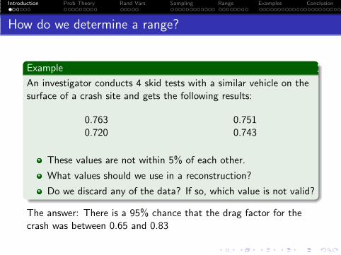
An investigator conducts 4 skid tests with a similar vehicle on thesurface of a crash site and gets the following results:
0.7630.720
0.7510.743
These values are not within 5% of each other.
What values should we use in a reconstruction?
Do we discard any of the data? If so, which value is not valid?
The answer: There is a 95% chance that the drag factor for thecrash was between 0.65 and 0.83

Introduction Prob Theory Rand Vars Sampling Range Examples Conclusion
How do we determine a range?
Example
An investigator conducts 4 skid tests with a similar vehicle on thesurface of a crash site and gets the following results:
0.7630.720
0.7510.743
These values are not within 5% of each other.
What values should we use in a reconstruction?
Do we discard any of the data? If so, which value is not valid?
The answer: There is a 95% chance that the drag factor for thecrash was between 0.65 and 0.83

Introduction Prob Theory Rand Vars Sampling Range Examples Conclusion
Motivation
Crash Reconstruction by nature is highly variable.
Statistics provide some tools to help us quantify the variationfound in crash reconstruction.
All calculations can be performed with a spreadsheet.A preprogrammed spreadsheet is publically available athttp://www.jhscientific.com/cgi-bin/downloads.py.
We can deal with both large samples and small samples.
Experience DOES matter! Mathematics does not turn baddata into good data. All answers should be checked.

Introduction Prob Theory Rand Vars Sampling Range Examples Conclusion
Two Types of Uncertainty
Aleatory uncertainty describes the inherent variationassociated with the physical system. This is alsocalled the noise in a system.
Epistemic uncertainty is a result of our ignorance. This can beeither because we lack enough data or ourmathematical models are not good enough. If wecollect more data, our understanding improves.
We will have one tool that deals with both types of uncertainty.

Introduction Prob Theory Rand Vars Sampling Range Examples Conclusion
Statistics Definitions
Stochastic is a term given to a quantity (variable) that neverhas one specific value. Its values are represented by aprobability function.
Deterministic is the converse to stochastic in that the value of adeterministic quantity is unique for a given situation.
Constants are parameters that never change. For our purposes,the acceleration due to gravity is a constant 32.2ft/s2.

Introduction Prob Theory Rand Vars Sampling Range Examples Conclusion
Stochastic Variables
What are some common quantities in reconstruction that arestochastic?
Drag Factor
Crush Stiffness Coefficients
Human Performance
Walking SpeedsPerception TimeReaction Time
Some variables are difficult to quantify using statistics
Departure angles from a crashTake off angle for an airborne analysis
Always make sure the result of a statistical analysis makessense given the physical evidence!!

Introduction Prob Theory Rand Vars Sampling Range Examples Conclusion
Probability and Statistics
Statistics is the art of learning from data.
Probability theory provides the framework to discuss theinterpretation of the data.

Introduction Prob Theory Rand Vars Sampling Range Examples Conclusion
Probability and Statistics
Statistics is the art of learning from data.
Probability theory provides the framework to discuss theinterpretation of the data.

Introduction Prob Theory Rand Vars Sampling Range Examples Conclusion
Outline
1 IntroductionMotivationStatistical Definitions
2 Probability TheoryAxioms of ProbabilityConditional ProbabilityBayes’ Theorem
3 Random VariablesNormal DistributionCentral Limit Theorem
4 SamplingDescriptive Statistics
Statistics for the MeanStatistics for the Variance
5 Determining a RangeFrequentist AssumptionsSignificance levelsThe Bootstrapping Method
6 ExamplesDrag FactorsCrush Stiffness CoefficientsPerception-Reaction TimeWalking SpeedsDrag Sleds vs. Accelerometers
7 Conclusion

Introduction Prob Theory Rand Vars Sampling Range Examples Conclusion
What is Probability?
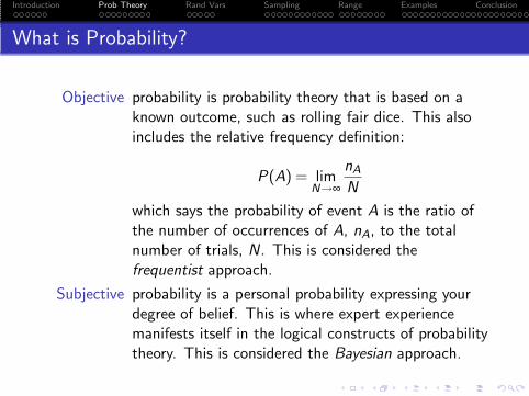
Objective probability is probability theory that is based on aknown outcome, such as rolling fair dice. This alsoincludes the relative frequency definition:
P(A) = limN→∞
nA
N
which says the probability of event A is the ratio ofthe number of occurrences of A, nA, to the totalnumber of trials, N. This is considered thefrequentist approach.
Subjective probability is a personal probability expressing yourdegree of belief. This is where expert experiencemanifests itself in the logical constructs of probabilitytheory. This is considered the Bayesian approach.
Introduction Prob Theory Rand Vars Sampling Range Examples Conclusion
What is Probability?
Objective probability is probability theory that is based on aknown outcome, such as rolling fair dice. This alsoincludes the relative frequency definition:
P(A) = limN→∞
nA
N
which says the probability of event A is the ratio ofthe number of occurrences of A, nA, to the totalnumber of trials, N. This is considered thefrequentist approach.
Subjective probability is a personal probability expressing yourdegree of belief. This is where expert experiencemanifests itself in the logical constructs of probabilitytheory. This is considered the Bayesian approach.

Introduction Prob Theory Rand Vars Sampling Range Examples Conclusion
Axioms of Probability
1 The probability of an event is represented as a numberbetween 0 and 1.
If the probability of an event is 0, then the event will neverhappen.If the probability of an event is 1, then the event will alwaysoccur.
2 The probability of all events must add to 1
3 The probability of two independent events is the sum of theirindividual probabilities.
Introduction Prob Theory Rand Vars Sampling Range Examples Conclusion
An Example of a Die
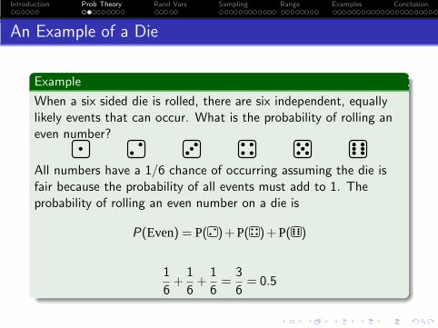
Example
When a six sided die is rolled, there are six independent, equallylikely events that can occur. What is the probability of rolling aneven number?
All numbers have a 1/6 chance of occurring assuming the die isfair because the probability of all events must add to 1. Theprobability of rolling an even number on a die is
P(Even) = P( )+P( )+P( )
1
6+
1
6+
1
6=
3
6= 0.5

Introduction Prob Theory Rand Vars Sampling Range Examples Conclusion
Conditional Probability
Definition
Conditional probability has very logical basis. The notation P(A|B)says the probability of event A given event B. This allows us tocondition the probability given some event.
P(A|B) =P(A and B)
P(B)

Introduction Prob Theory Rand Vars Sampling Range Examples Conclusion
Rolling the Dice
Example
Consider rolling two dice, one at a time. What is the probability ofgetting a 3?A three can happen one of two ways: Either or . Theprobability is written mathematically as:
P( and ) or P( and )
P( )×P( )+P( )×P( )(
1
6
)(1
6
)
+
(1
6
)(1
6
)
=2
36

Introduction Prob Theory Rand Vars Sampling Range Examples Conclusion
Rolling the Dice
Example
What if we roll one die at a time and the first die shows up ?Now the probability of getting a three has changed. It is nowconditional.
P(3| ) =P(3 and )
P( )
=13616
=1
6
The probability of the final outcome is conditioned by the resultsof the first event.
Introduction Prob Theory Rand Vars Sampling Range Examples Conclusion
Conditional Probability
Theorem
The probability every real world event is conditional, even if onlyon background information.
Proof.
Every real event was influenced by either the previous event or thesurroundings. Our belief of events in a crash depend on ourexperience and the evidence at the scene.

Introduction Prob Theory Rand Vars Sampling Range Examples Conclusion
Conditional Probability
Example
The probability of a vehicle negotiating a turn depends on theradius of the turn and the friction of the road. The friction isdependent on the weather and the weather is dependent on theseason and so forth.
Conditional probability that includes background information iswritten as:
P(A|B, I )
The background information is always present in an analysis andmust be understood.

Introduction Prob Theory Rand Vars Sampling Range Examples Conclusion
Bayes’ Theorem
Theorem
Bayes’ theory allows us to work with conditional probabilities:
P(A|B) =P(B|A)P(A)
P(B|A)P(A)+P(B|not A)P(not A)
This can lead to a discussion of joint and marginal probability (offtopic).

Introduction Prob Theory Rand Vars Sampling Range Examples Conclusion
Priors, Posteriors and Likelihood
Simplify Bayes’ Theorem:
P(Event|Data, I ) ∝ P(Data|Event, I )P(Event|I )
I is the background information
P(Event|I ) is the prior probability
P(Data|Event, I ) is the likelihood function
P(Event|Data, I ) is the posterior probability
We can combine our knowledge with test results to get a newdistribution.What is a probability distribution function?

Introduction Prob Theory Rand Vars Sampling Range Examples Conclusion
Outline
1 IntroductionMotivationStatistical Definitions
2 Probability TheoryAxioms of ProbabilityConditional ProbabilityBayes’ Theorem
3 Random VariablesNormal DistributionCentral Limit Theorem
4 SamplingDescriptive Statistics
Statistics for the MeanStatistics for the Variance
5 Determining a RangeFrequentist AssumptionsSignificance levelsThe Bootstrapping Method
6 ExamplesDrag FactorsCrush Stiffness CoefficientsPerception-Reaction TimeWalking SpeedsDrag Sleds vs. Accelerometers
7 Conclusion
Introduction Prob Theory Rand Vars Sampling Range Examples Conclusion
Random Variables
Definition
A random variable is the numerical outcome of a randomexperiment.
An event needs to be coded or operationalized to become arandom variable.
Some random events have little meaning as random variables.Examples: driver fatigue or human emotion
Random variables are described in terms of probabilitydistributions.

Introduction Prob Theory Rand Vars Sampling Range Examples Conclusion
The Normal Distribution
f (x)
µ µ +σµ −σ
Figure: The probability density function of a Normal distribution with amean of µ (mu) and a standard deviation of σ (sigma). The shadedregion represents 68% of the area and is bounded by ±1σ . The area isequal to the probability.

Introduction Prob Theory Rand Vars Sampling Range Examples Conclusion
The Normal Distribution
Definition
The equation for the probability density function (PDF) of theNormal (Gaussian) distribution is:
f (x) =1
σ√
2πexp
(
−1
2
[x −µ
σ
]2)
It is written shorthand as N(µ,σ).

Introduction Prob Theory Rand Vars Sampling Range Examples Conclusion
Normal Distributions Representing Drag Factor
Example
Plot the Probability Density Functions (PDFs) of the drag factorsfor a new Crown Victoria and an old 3/4 ton Pickup. The PDF ofthe Crown Victoria is:
N(0.8,0.03)
The PDF of the Pickup is:
N(0.6,0.08)

Introduction Prob Theory Rand Vars Sampling Range Examples Conclusion
Normal Distributions Representing Drag Factor
0.8f
0.6
Figure: The normal distribution representing the truck has a lower meanbut more spread.

Introduction Prob Theory Rand Vars Sampling Range Examples Conclusion
Central Limit Theorem
Why do we use a normal distribution?
Theorem
Variables that are influenced by many different factors that areunrelated approximate a normal distribution.
Note: Normal distributions are found in all aspects of physicalphenomena. They are the most likely distributions given no otherinformation.

Introduction Prob Theory Rand Vars Sampling Range Examples Conclusion
Outline
1 IntroductionMotivationStatistical Definitions
2 Probability TheoryAxioms of ProbabilityConditional ProbabilityBayes’ Theorem
3 Random VariablesNormal DistributionCentral Limit Theorem
4 SamplingDescriptive Statistics
Statistics for the MeanStatistics for the Variance
5 Determining a RangeFrequentist AssumptionsSignificance levelsThe Bootstrapping Method
6 ExamplesDrag FactorsCrush Stiffness CoefficientsPerception-Reaction TimeWalking SpeedsDrag Sleds vs. Accelerometers
7 Conclusion
Introduction Prob Theory Rand Vars Sampling Range Examples Conclusion
Sampling from a Population
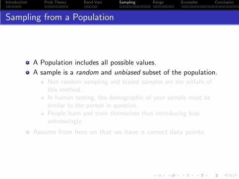
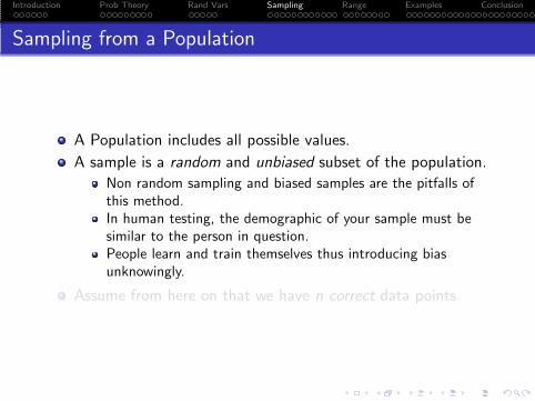
A Population includes all possible values.
A sample is a random and unbiased subset of the population.
Non random sampling and biased samples are the pitfalls ofthis method.In human testing, the demographic of your sample must besimilar to the person in question.People learn and train themselves thus introducing biasunknowingly.
Assume from here on that we have n correct data points.
Introduction Prob Theory Rand Vars Sampling Range Examples Conclusion
Sampling from a Population
A Population includes all possible values.
A sample is a random and unbiased subset of the population.
Non random sampling and biased samples are the pitfalls ofthis method.In human testing, the demographic of your sample must besimilar to the person in question.People learn and train themselves thus introducing biasunknowingly.
Assume from here on that we have n correct data points.

Introduction Prob Theory Rand Vars Sampling Range Examples Conclusion
The Sample Mean
Definition
The sample mean, x is the arithmetic average of the data:
x =x1 + x2 + x3 + · · ·+ xn
n
This is also written as:
x =∑n
i=1 xi
n
where ∑ is the summation symbol and means to add all the itemsin the list together.
In Excel: =AVERAGE(array)

Introduction Prob Theory Rand Vars Sampling Range Examples Conclusion
The Sample Standard Deviation
Definition
The sample variance, s2 is obtained with the following formula:
s2 =(x1− x)2 +(x2− x)2 + · · ·+(xn − x)2
n−1
This is also written as:
s2 =∑n
i=1(xi − x)2
n−1
The standard deviation is the square root of the variance:
s =
√
∑ni=1(xi − x)2
n−1
In Excel: =STDEV(array) and =VAR(array)

Introduction Prob Theory Rand Vars Sampling Range Examples Conclusion
Other Descriptions of Data
Central Tendency
Median: 50th percentileMode: the most frequentFor a symmetric distribution: mean = median = mode
Measures of Spread
RangePercentilesBox and Whisker Plots

Introduction Prob Theory Rand Vars Sampling Range Examples Conclusion
Drag Factor Example
Example
The sample mean, x of the given data is:
x =0.763+0.720+0.751+0.743
4= 0.744
The sample variance is:
s2 = VAR(0.763,0.720,0.751,0.743) = 0.0003289
The sample standard deviation is:
s =√
0.0003289 = 0.01814

Introduction Prob Theory Rand Vars Sampling Range Examples Conclusion
Estimators
The sample mean and sample standard deviation are the mostlikely estimates of the true population mean and true populationstandard deviation.
x ⇐⇒ µs ⇐⇒ σ
Since these sample statistics are just estimates, the true populationparameters follow some distribution with respect to their respectiveestimators.

Introduction Prob Theory Rand Vars Sampling Range Examples Conclusion
Distribution of the Mean
Theorem
The distribution of sample means follow a Student-t distributionthat considers the number of samples in the data– regardless ofthe underlying distribution.
x −µs/√
n∼ tn,α
where the term s/√
n is called the standard error.
Note:
As the number of samples becomes large, the standard error dropsto zero and the sample mean approaches the true mean.
Introduction Prob Theory Rand Vars Sampling Range Examples Conclusion
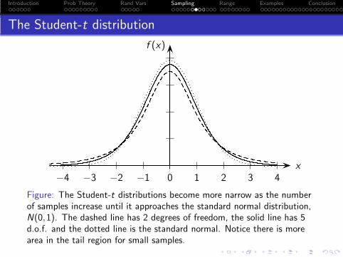
The Student-t distribution
0 1 2 3 4−1−2−3−4x
f (x)
Figure: The Student-t distributions become more narrow as the numberof samples increase until it approaches the standard normal distribution,N(0,1). The dashed line has 2 degrees of freedom, the solid line has 5d.o.f. and the dotted line is the standard normal. Notice there is morearea in the tail region for small samples.

Introduction Prob Theory Rand Vars Sampling Range Examples Conclusion
An Example of the Distribution of the Mean
Example
Construct the two sided confidence interval for the mean of the 4drag factor samples at the α = 0.05 significance level.We can write the distribution of the true population mean as:
µ = x + t4,0.05
(s√n
)
The standard error is:
s√n
=0.01814√
4= 0.009068

Introduction Prob Theory Rand Vars Sampling Range Examples Conclusion
A Picture of the Distribution of the Mean
0.64 0.66 0.68 0.70 0.72 0.74 0.76 0.78 0.80
µ
x = 0.744
Figure: The distribution of the mean follows a Student-t distribution. Forthis example the critical t value for 4 dof and 95% confidence is 2.7764.This gives a confidence bound on the mean as 0.744±2.7764(0.009068)which is a bound between 0.719 and 0.769.
Note:
The critical t value is computed in Excel as =TINV(.05,4)

Introduction Prob Theory Rand Vars Sampling Range Examples Conclusion
The Distribution of the Variance
We have only examined the mean. What about the variance (std.dev.)?
Theorem
The distribution of the true variance follows a χ2 (chi-squared)distribution:
(n−1)s2
σ2∼ χ2
n−1
Where the χ2 distribution depends on the degrees of freedom(n−1). The mean and standard deviation of a χ2
n−1 distributionare:
µ = n−1
σ2 = 2(n−1)
Introduction Prob Theory Rand Vars Sampling Range Examples Conclusion
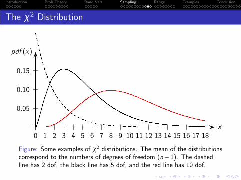
The χ2 Distribution
0.05
0.10
0.15
0 1 2 3 4 5 6 7 8 9 10 11 12 13 14 15 16 17 18
x
pdf (x)
Figure: Some examples of χ2 distributions. The mean of the distributionscorrespond to the numbers of degrees of freedom (n−1). The dashedline has 2 dof, the black line has 5 dof, and the red line has 10 dof.
Introduction Prob Theory Rand Vars Sampling Range Examples Conclusion
An Example of the Distribution of the Variance
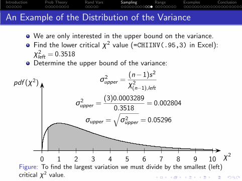
We are only interested in the upper bound on the variance.Find the lower critical χ2 value (=CHIINV(.95,3) in Excel):χ2
left = 0.3518Determine the upper bound of the variance:
σ2upper =
(n−1)s2
χ2(n−1),left
σ2upper =
(3)0.0003289
0.3518= 0.002804
σupper =√
σ2upper = 0.05296
0 1 2 3 4 5 6 7 8 9 10 χ2
pdf (χ2)
Figure: To find the largest variation we must divide by the smallest (left)critical χ2 value.

Introduction Prob Theory Rand Vars Sampling Range Examples Conclusion
Outline
1 IntroductionMotivationStatistical Definitions
2 Probability TheoryAxioms of ProbabilityConditional ProbabilityBayes’ Theorem
3 Random VariablesNormal DistributionCentral Limit Theorem
4 SamplingDescriptive Statistics
Statistics for the MeanStatistics for the Variance
5 Determining a RangeFrequentist AssumptionsSignificance levelsThe Bootstrapping Method
6 ExamplesDrag FactorsCrush Stiffness CoefficientsPerception-Reaction TimeWalking SpeedsDrag Sleds vs. Accelerometers
7 Conclusion

Introduction Prob Theory Rand Vars Sampling Range Examples Conclusion
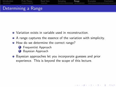
Determining a Range
Variation exists in variable used in reconstruction.
A range captures the essence of the variation with simplicity.
How do we determine the correct range?1 Frequentist Approach2 Bayesian Approach
Bayesian approaches let you incorporate guesses and priorexperience. This is beyond the scope of this lecture.

Introduction Prob Theory Rand Vars Sampling Range Examples Conclusion
Determining a Range
Variation exists in variable used in reconstruction.
A range captures the essence of the variation with simplicity.
How do we determine the correct range?1 Frequentist Approach2 Bayesian Approach
Bayesian approaches let you incorporate guesses and priorexperience. This is beyond the scope of this lecture.

Introduction Prob Theory Rand Vars Sampling Range Examples Conclusion
Frequentist (Classical) Assumptions
The population of samples is Normally distributed.
Every sample is independent of all other samples.
Every sample comes from the same parent distribution.
The mean and standard deviation of the parent population areunknown.

Introduction Prob Theory Rand Vars Sampling Range Examples Conclusion
Significance Levels
Definition
The significance level is the amount of probability that aproposition is not true. We denote the significance as α . Thischoice is arbitrary but the commonly used significance levels areα = 0.10, α = 0.05, and, α = 0.01.
We use this definition to determine the most likely intervals of aparticular value.

Introduction Prob Theory Rand Vars Sampling Range Examples Conclusion
Two Tails or One Tail
x
f (x)
µ µ +1.645σ
(a) A one sided confidence interval
x
f (x)
µ µ +1.96σµ −1.96σ
(b) A two sided confidence interval
Figure: The difference in a one sided and two sided confidence interval.In each case 95% of the area is enclosed.
Introduction Prob Theory Rand Vars Sampling Range Examples Conclusion
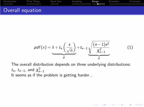
Overall equation
pdf (x) = x + tn
(s√n
)
︸ ︷︷ ︸
µ
+tn−1
√
(n−1)s2
χ2n−1
︸ ︷︷ ︸
σ
(1)
The overall distribution depends on three underlying distributions:tn, tn−1, and χ2
n−1
It seems as if the problem is getting harder...
Introduction Prob Theory Rand Vars Sampling Range Examples Conclusion
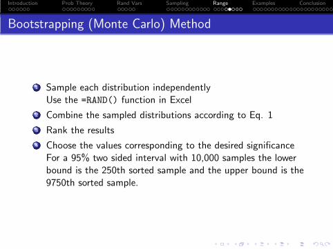
Bootstrapping (Monte Carlo) Method
1 Sample each distribution independentlyUse the =RAND() function in Excel
2 Combine the sampled distributions according to Eq. 1
3 Rank the results
4 Choose the values corresponding to the desired significanceFor a 95% two sided interval with 10,000 samples the lowerbound is the 250th sorted sample and the upper bound is the9750th sorted sample.

Introduction Prob Theory Rand Vars Sampling Range Examples Conclusion
A Picture of the Range
Emperical Cummulative Probability
0
0.1
0.2
0.3
0.4
0.5
0.6
0.7
0.8
0.9
1
0.6 0.65 0.7 0.75 0.8 0.85 0.9
Drag Factor
CD
F
Monte Carlo CDF
Range
Figure: The result of the Monte Carlo simulation represented as acumulative distribution. The actual value has a 95% chance of lying inthe range shown above.

Introduction Prob Theory Rand Vars Sampling Range Examples Conclusion
Range Estimation of a Normally Distributed Variable With an Unknown Mean
and Unknown Standard Deviation
Label Example Drag Factor Tests
Data 0.763
0.720
0.751
0.743
Summary Statistics
Count 4
Sample Mean 0.744
Sample Std Dev 0.01814
Standard Error 0.009068030
Variance 0.0003289167
Significance 95%
alpha 0.05 (this can be changed)
Confidence Interval for the Mean
Student-t 2.7764 (two tailed)
Low Mean 0.7191
High Mean 0.7694
Upper Bound on the Variance
Chi Squared Left 0.351846 (one sided)
Max Variance 0.002804
Max Stdev 0.052957
Bootstrap (Monte Carlo) Results (use this range if it makes sense)
lower bound 0.653upper bound 0.833
Significance Bounds on Most Likely Normal Distribution
lower bound 0.709
upper bound 0.780 (this is computed from summary Stats)
Difference (should be positive)
upper bound 0.055450
lower bound 0.053324
Instructions For Use:
1.) Enter the Desired Data in Column B
2.) Adjust the Value of alpha as Desired (0.05 is commonly accepted)
3.) Press F9 to Calculate the Worksheet (Calculation takes a long time)
Note: The Monte Carlo results may change slightly with each calculation

Introduction Prob Theory Rand Vars Sampling Range Examples Conclusion
Concluding Our Example
The results of the simulation for our drag factor data are:
flower = 0.65
fupper = 0.83
For a 100 ft slide to stop the calculated speeds would be from44.83 mph to 49.59 mph.

Introduction Prob Theory Rand Vars Sampling Range Examples Conclusion
Outline
1 IntroductionMotivationStatistical Definitions
2 Probability TheoryAxioms of ProbabilityConditional ProbabilityBayes’ Theorem
3 Random VariablesNormal DistributionCentral Limit Theorem
4 SamplingDescriptive Statistics
Statistics for the MeanStatistics for the Variance
5 Determining a RangeFrequentist AssumptionsSignificance levelsThe Bootstrapping Method
6 ExamplesDrag FactorsCrush Stiffness CoefficientsPerception-Reaction TimeWalking SpeedsDrag Sleds vs. Accelerometers
7 Conclusion

Introduction Prob Theory Rand Vars Sampling Range Examples Conclusion
Another Drag Factor Example
Example
Consider three skid tests from an accelerometer mounted in anexemplar vehicle. What range of the drag factor should be used ifthe three readings are 0.786, 0.812, and 0.794? Let x denote thedrag factor.
Note:
These measurements are within 5%.

Introduction Prob Theory Rand Vars Sampling Range Examples Conclusion
Range Estimation of a Normally Distributed Variable With an Unknown Mean
and Unknown Standard Deviation
Label Example Drag Factor Tests
Data 0.786
0.812
0.794
Summary Statistics
Count 3
Sample Mean 0.797
Sample Std Dev 0.01332
Standard Error 0.00769
Variance 0.00018
Significance 95%
alpha 0.05 (this can be changed)
Confidence Interval for the Mean
Student-t 3.1824 (two tailed)
Low Mean 0.7729
High Mean 0.8218
Upper Bound on the Variance
Chi Squared Left 0.1026 (one sided)
Max Variance 0.00346
Max Stdev 0.05880
Bootstrap (Monte Carlo) Results (use this range if it makes sense)
lower bound 0.684upper bound 0.911
Significance Bounds on Most Likely Normal Distribution
lower bound 0.771
upper bound 0.823 (this is computed from summary Stats)
Difference (should be positive)
upper bound 0.087091
lower bound 0.087377
Instructions For Use:
1.) Enter the Desired Data in Column B
2.) Adjust the Value of alpha as Desired (0.05 is commonly accepted)
3.) Press F9 to Calculate the Worksheet (Calculation takes a long time)
Note: The Monte Carlo results may change slightly with each calculation

Introduction Prob Theory Rand Vars Sampling Range Examples Conclusion
Summary Statistics
Sample mean:
x =0.786+0.812+0.794
3= 0.797
Sample Variance:
s2 =(0.786−0.797)2 +(0.812−0.797)2 +(0.794−0.797)2
3−1=0.00018
Sample Standard Deviation:
s =√
s2 = 0.01332
Standard Error:
StdErr =0.01332√
3= 0.00769

Introduction Prob Theory Rand Vars Sampling Range Examples Conclusion
Confidence Interval on the Mean
Specify the significance level: α = 0.05
Find the critical t value (=TINV(Prob,DOF) in Excel):tcrit = 3.182
µ
pdf (µ)
xx −3.182 s√n
x +3.182 s√n
Figure: The 95% confidence interval for the mean is 0.797±0.0244.

Introduction Prob Theory Rand Vars Sampling Range Examples Conclusion
Confidence Bound on the Variance
We are only interested in the upper bound on the variance.
Find the lower critical χ2 value (=CHIINV(Prob,DOF) inExcel): χ2
left = 0.1026
Determine the upper bound of the variance:
σ2upper =
(n−1)s2
χ2(n−1),left
σ2upper =
(2)0.000177
0.1026= 0.00345
σupper =√
σ2upper = 0.0588
0 1 2 3 4 5 6 7 8 9 10 χ2
pdf (χ2)

Introduction Prob Theory Rand Vars Sampling Range Examples Conclusion
Run Monte Carlo on Overall Equation
Evaluate 10,000 trials of the equation
Rank all 10,000 results
Extract the 250th and 9750th result to create a range.
Emperical Cummulative Probability
0
0.1
0.2
0.3
0.4
0.5
0.6
0.7
0.8
0.9
1
0.5 0.6 0.7 0.8 0.9 1 1.1
Drag Factor
CD
F
Range
Figure: The result of the Monte Carlo simulation represented as acumulative distribution. The range extracted is 0.68 to 0.91.

Introduction Prob Theory Rand Vars Sampling Range Examples Conclusion
The Range from the Most Likely Normal Distribution
The range given from the normal distribution with a mean of xand a standard deviation of s will always be tighter than previouslydetermined.
For our example x is the drag factor:
55 0.60 0.65 0.70 0.75 0.80 0.85 0.90
x
x
Figure: The shaded region represents 95% of the area and is bounded byx ±1.96s. This gives the lower bound of 0.771 and the upper bound is0.823. This technique does not account for any uncertianty in the meanor standard deviation.

Introduction Prob Theory Rand Vars Sampling Range Examples Conclusion
Crush Stiffness
We can use this for more than drag factors...
Example
A query of the StifCalcs database for 1991-1993 frontal crash testdata for the Honda Accord provided the following data for the Astiffness coefficient values:
354.7600.0649.7362.4908.2353.6386.7
578.9364.2424.9620.2857.1553.5627.6
936.8311.4624.6601.5752.4405.2326.7
703.6320.9347.3332.8328.1
Let’s determine a range to use in an analysis using thespreadsheet...

Introduction Prob Theory Rand Vars Sampling Range Examples Conclusion
Range Estimation of a Normally Distributed Variable With an Unknown Mean
and Unknown Standard Deviation
Label A Stiffness 4N6XPRT StifCalcs for 1991-1993 Honda Accord Frontal Impacts
Data 354.7
600
649.7
362.4
908.2
353.6
386.7 Summary Statistics
578.9 Count 26
364.2 Sample Mean 523.577
424.9 Sample Std Dev 195.740
620.2 Standard Error 38.388
857.1 Variance 38313.980
533.5
627.6 Significance 95%
936.8 alpha 0.05 (this can be changed)
311.4
624.6 Confidence Interval for the Mean
601.5 Student-t 2.06 (two tailed)
752.4 Low Mean 444.67
405.2 High Mean 602.48
326.7
703.6 Upper Bound on the Variance
320.9 Chi Squared Left 14.611 (one sided)
347.3 Max Variance 65554.909
332.8 Max Stdev 256.037
328.1
Bootstrap (Monte Carlo) Results (use this range if it makes sense)
lower bound 89.180upper bound 960.394
Significance Bounds on Most Likely Normal Distribution
lower bound 139.934
upper bound 907.219 (this is computed from summary Stats)
Difference (should be positive)
upper bound 50.754559
lower bound 53.174982
Instructions For Use:
1.) Enter the Desired Data in Column B
2.) Adjust the Value of alpha as Desired (0.05 is commonly accepted)
3.) Press F9 to Calculate the Worksheet (Calculation takes a long time)
Note: The Monte Carlo results may change slightly with each calculation

Introduction Prob Theory Rand Vars Sampling Range Examples Conclusion
Problem: Huge Scatter
1 The spreadsheet gives the following:
Alow = 89.18 lb/in
Ahigh = 960.39 lb/in
2 The range is absurd!!
Ratio of s to x is largeUnderlying distribution does not follow a Normal Distribution
3 Further investigation reveals that the data included vehicle tovehicle data combined with vehicle to barrier data.
4 Cannot take samples from two different populations.
Note:
Excessive ranges indicate improper data or testing techniques. Inthis case, check the original crash test reports and ensure the samephysical process is being measured.

Introduction Prob Theory Rand Vars Sampling Range Examples Conclusion
Are These Data Normal?
Comparison of the Cumulative Probability Functions
0
0.1
0.2
0.3
0.4
0.5
0.6
0.7
0.8
0.9
1
0 200 400 600 800 1000 1200
A Stiffness Coefficient
Cu
mu
lati
ve P
rob
ab
ilit
y (
CD
F)
Normal CDF
A Coeff Emperical CDF
Figure: The actual data are sorted and ranked. Their ranking is dividedby n+1 to get the percentile (probability). The plot of the percentile(empirical CDF) is compared to the plot of the Normal CDF[=NORMINV(prob,mean,stddev)]. These data do not appear to benormally distributed. (There are two different populations.)

Introduction Prob Theory Rand Vars Sampling Range Examples Conclusion
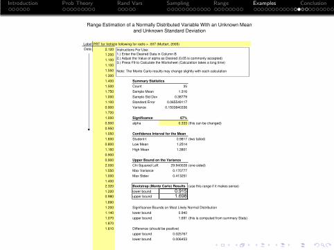
Perception-Reaction Time Example
Adjusted Perception-Reaction time was measured for a vehiclefollowing situation.
The data were taken from [Muttart, 2005] and entered intothe spreadsheet.
A normal driver was defined as the driver in the middle twothirds so α = 1/3.
Results for 66%, 95% are compared.
Plots of the CDF are plotted.

Introduction Prob Theory Rand Vars Sampling Range Examples Conclusion
Perception-Reaction Time Example
Adjusted Perception-Reaction time was measured for a vehiclefollowing situation.
The data were taken from [Muttart, 2005] and entered intothe spreadsheet.
A normal driver was defined as the driver in the middle twothirds so α = 1/3.
Results for 66%, 95% are compared.
Plots of the CDF are plotted.
Introduction Prob Theory Rand Vars Sampling Range Examples Conclusion
Range Estimation of a Normally Distributed Variable With an Unknown Mean
and Unknown Standard Deviation
Label PRT for Vehicle following for rad/s > .007 (Muttart, 2005)
Data 2.120
1.200
1.100
1.100
1.550
1.300
1.400 Summary Statistics
1.500 Count 35
1.750 Sample Mean 1.316
1.000 Sample Std Dev 0.38779
1.100 Standard Error 0.065549117
0.900 Variance 0.1503840336
1.720
1.000 Significance 67%
0.900 alpha 0.333 (this can be changed)
0.950
1.050 Confidence Interval for the Mean
1.600 Student-t 0.9817 (two tailed)
0.800 Low Mean 1.2514
1.160 High Mean 1.3801
0.900
0.900 Upper Bound on the Variance
2.000 Chi Squared Left 29.940028 (one sided)
1.550 Max Variance 0.170777
1.000 Max Stdev 0.413251
1.400
2.320 Bootstrap (Monte Carlo) Results (use this range if it makes sense)
1.220 lower bound 0.9150.980 upper bound 1.698
1.690
1.200 Significance Bounds on Most Likely Normal Distribution
1.140 lower bound 0.940
1.070 upper bound 1.691 (this is computed from summary Stats)
1.870
1.610 Difference (should be positive)
upper bound 0.025767
lower bound 0.006453
Instructions For Use:
1.) Enter the Desired Data in Column B
2.) Adjust the Value of alpha as Desired (0.05 is commonly accepted)
3.) Press F9 to Calculate the Worksheet (Calculation takes a long time)
Note: The Monte Carlo results may change slightly with each calculation

Introduction Prob Theory Rand Vars Sampling Range Examples Conclusion
Range Estimation of a Normally Distributed Variable With an Unknown Mean
and Unknown Standard Deviation
Label PRT for Vehicle following for rad/s > .007 (Muttart, 2005)
Data 2.120
1.200
1.100
1.100
1.550
1.300
1.400 Summary Statistics
1.500 Count 35
1.750 Sample Mean 1.316
1.000 Sample Std Dev 0.38779
1.100 Standard Error 0.065549117
0.900 Variance 0.1503840336
1.720
1.000 Significance 95%
0.900 alpha 0.05 (this can be changed)
0.950
1.050 Confidence Interval for the Mean
1.600 Student-t 2.0301 (two tailed)
0.800 Low Mean 1.1826
1.160 High Mean 1.4488
0.900
0.900 Upper Bound on the Variance
2.000 Chi Squared Left 21.664281 (one sided)
1.550 Max Variance 0.236013
1.000 Max Stdev 0.485812
1.400
2.320 Bootstrap (Monte Carlo) Results (use this range if it makes sense)
1.220 lower bound 0.4810.980 upper bound 2.157
1.690
1.200 Significance Bounds on Most Likely Normal Distribution
1.140 lower bound 0.556
1.070 upper bound 2.076 (this is computed from summary Stats)
1.870
1.610 Difference (should be positive)
upper bound 0.074273
lower bound 0.081157
Instructions For Use:
1.) Enter the Desired Data in Column B
2.) Adjust the Value of alpha as Desired (0.05 is commonly accepted)
3.) Press F9 to Calculate the Worksheet (Calculation takes a long time)
Note: The Monte Carlo results may change slightly with each calculation

Introduction Prob Theory Rand Vars Sampling Range Examples Conclusion
Are PRT Data Normal?
Cumulative Probability of Vehicle Following PRT
0
0.1
0.2
0.3
0.4
0.5
0.6
0.7
0.8
0.9
1
0.000 0.500 1.000 1.500 2.000 2.500 3.000
Perception-Reaction Time
Cu
mu
lati
ve P
rob
ab
ilit
y
Emperical
Normal
LogNormal
Figure: The actual data are sorted and ranked. Their ranking is dividedby n+1 to get the percentile (probability). The plot of the percentile(empirical CDF) is compared to the plot of the Normal CDF[=NORMINV(prob,mean,stddev)]. A log normal CDF is also shown.These data are near normal.

Introduction Prob Theory Rand Vars Sampling Range Examples Conclusion
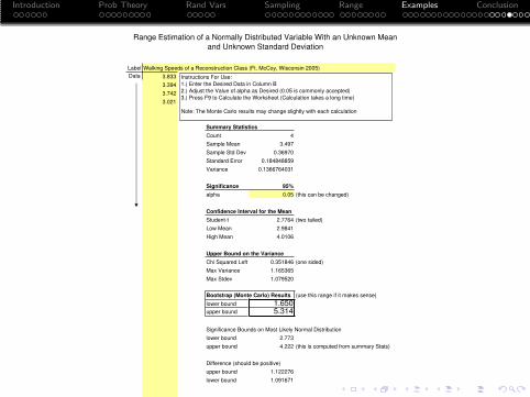
Examine Walking Speeds for Insight on Sample Size
Walking speeds were measured of a reconstruction class(Wisconsin 2002)
Pedestrians were timed walking 100 ft
Average walking speeds were computed in mph for eachparticipant
The data was analyzed unsorted (as it was obtained)
Example
Perform the range analysis for data sets of different sizes.

Introduction Prob Theory Rand Vars Sampling Range Examples Conclusion
Range Estimation of a Normally Distributed Variable With an Unknown Mean
and Unknown Standard Deviation
Label Walking Speeds of a Reconstruction Class (Ft. McCoy, Wisconsin 2005)
Data 3.833
3.394
Summary Statistics
Count 2
Sample Mean 3.613
Sample Std Dev 0.31026
Standard Error 0.219386820
Variance 0.0962611539
Significance 95%
alpha 0.05 (this can be changed)
Confidence Interval for the Mean
Student-t 4.3027 (two tailed)
Low Mean 2.6693
High Mean 4.5572
Upper Bound on the Variance
Chi Squared Left 0.003932 (one sided)
Max Variance 24.480602
Max Stdev 4.947788
Bootstrap (Monte Carlo) Results (use this range if it makes sense)
lower bound -13.350upper bound 16.270
Significance Bounds on Most Likely Normal Distribution
lower bound 3.005
upper bound 4.221 (this is computed from summary Stats)
Difference (should be positive)
upper bound 16.354855
lower bound 12.048829
Instructions For Use:
1.) Enter the Desired Data in Column B
2.) Adjust the Value of alpha as Desired (0.05 is commonly accepted)
3.) Press F9 to Calculate the Worksheet (Calculation takes a long time)
Note: The Monte Carlo results may change slightly with each calculation

Introduction Prob Theory Rand Vars Sampling Range Examples Conclusion
Range Estimation of a Normally Distributed Variable With an Unknown Mean
and Unknown Standard Deviation
Label Walking Speeds of a Reconstruction Class (Ft. McCoy, Wisconsin 2005)
Data 3.833
3.394
3.742
Summary Statistics
Count 3
Sample Mean 3.656
Sample Std Dev 0.23167
Standard Error 0.133756085
Variance 0.0536720707
Significance 95%
alpha 0.05 (this can be changed)
Confidence Interval for the Mean
Student-t 3.1824 (two tailed)
Low Mean 3.2305
High Mean 4.0819
Upper Bound on the Variance
Chi Squared Left 0.102587 (one sided)
Max Variance 1.046376
Max Stdev 1.022925
Bootstrap (Monte Carlo) Results (use this range if it makes sense)
lower bound 1.567upper bound 5.545
Significance Bounds on Most Likely Normal Distribution
lower bound 3.202
upper bound 4.110 (this is computed from summary Stats)
Difference (should be positive)
upper bound 1.634991
lower bound 1.434837
Instructions For Use:
1.) Enter the Desired Data in Column B
2.) Adjust the Value of alpha as Desired (0.05 is commonly accepted)
3.) Press F9 to Calculate the Worksheet (Calculation takes a long time)
Note: The Monte Carlo results may change slightly with each calculation
Introduction Prob Theory Rand Vars Sampling Range Examples Conclusion
Range Estimation of a Normally Distributed Variable With an Unknown Mean
and Unknown Standard Deviation
Label Walking Speeds of a Reconstruction Class (Ft. McCoy, Wisconsin 2005)
Data 3.833
3.394
3.742
3.021
Summary Statistics
Count 4
Sample Mean 3.497
Sample Std Dev 0.36970
Standard Error 0.184848859
Variance 0.1366764031
Significance 95%
alpha 0.05 (this can be changed)
Confidence Interval for the Mean
Student-t 2.7764 (two tailed)
Low Mean 2.9841
High Mean 4.0106
Upper Bound on the Variance
Chi Squared Left 0.351846 (one sided)
Max Variance 1.165365
Max Stdev 1.079520
Bootstrap (Monte Carlo) Results (use this range if it makes sense)
lower bound 1.650upper bound 5.314
Significance Bounds on Most Likely Normal Distribution
lower bound 2.773
upper bound 4.222 (this is computed from summary Stats)
Difference (should be positive)
upper bound 1.122276
lower bound 1.091671
Instructions For Use:
1.) Enter the Desired Data in Column B
2.) Adjust the Value of alpha as Desired (0.05 is commonly accepted)
3.) Press F9 to Calculate the Worksheet (Calculation takes a long time)
Note: The Monte Carlo results may change slightly with each calculation

Introduction Prob Theory Rand Vars Sampling Range Examples Conclusion
Range Estimation of a Normally Distributed Variable With an Unknown Mean
and Unknown Standard Deviation
Label Walking Speeds of a Reconstruction Class (Ft. McCoy, Wisconsin 2005)
Data 3.833
3.394
3.742
3.021
3.742
3.328
3.116 Summary Statistics
2.862 Count 8
Sample Mean 3.380
Sample Std Dev 0.36578
Standard Error 0.129322507
Variance 0.1337944855
Significance 95%
alpha 0.05 (this can be changed)
Confidence Interval for the Mean
Student-t 2.3060 (two tailed)
Low Mean 3.0815
High Mean 3.6779
Upper Bound on the Variance
Chi Squared Left 2.167350 (one sided)
Max Variance 0.432123
Max Stdev 0.657361
Bootstrap (Monte Carlo) Results (use this range if it makes sense)
lower bound 2.315upper bound 4.487
Significance Bounds on Most Likely Normal Distribution
lower bound 2.663
upper bound 4.097 (this is computed from summary Stats)
Difference (should be positive)
upper bound 0.347738
lower bound 0.390736
Instructions For Use:
1.) Enter the Desired Data in Column B
2.) Adjust the Value of alpha as Desired (0.05 is commonly accepted)
3.) Press F9 to Calculate the Worksheet (Calculation takes a long time)
Note: The Monte Carlo results may change slightly with each calculation

Introduction Prob Theory Rand Vars Sampling Range Examples Conclusion
Range Estimation of a Normally Distributed Variable With an Unknown Mean
and Unknown Standard Deviation
Label Walking Speeds of a Reconstruction Class (Ft. McCoy, Wisconsin 2005)
Data 3.833
3.394
3.742
3.742
3.021
3.328
3.116 Summary Statistics
2.862 Count 12
3.339 Sample Mean 3.317
3.129 Sample Std Dev 0.31301
3.057 Standard Error 0.090359201
3.236 Variance 0.0979774229
Significance 95%
alpha 0.05 (this can be changed)
Confidence Interval for the Mean
Student-t 2.1788 (two tailed)
Low Mean 3.1197
High Mean 3.5135
Upper Bound on the Variance
Chi Squared Left 4.574813 (one sided)
Max Variance 0.235584
Max Stdev 0.485370
Bootstrap (Monte Carlo) Results (use this range if it makes sense)
lower bound 2.525upper bound 4.106
Significance Bounds on Most Likely Normal Distribution
lower bound 2.703
upper bound 3.930 (this is computed from summary Stats)
Difference (should be positive)
upper bound 0.177998
lower bound 0.175561
Instructions For Use:
1.) Enter the Desired Data in Column B
2.) Adjust the Value of alpha as Desired (0.05 is commonly accepted)
3.) Press F9 to Calculate the Worksheet (Calculation takes a long time)
Note: The Monte Carlo results may change slightly with each calculation

Introduction Prob Theory Rand Vars Sampling Range Examples Conclusion
Range Estimation of a Normally Distributed Variable With an Unknown Mean
and Unknown Standard Deviation
Label Walking Speeds of a Reconstruction Class (Ft. McCoy, Wisconsin 2005)
Data 3.833
3.394
3.742
3.742
3.021
3.328
3.116 Summary Statistics
2.862 Count 16
3.339 Sample Mean 3.240
3.129 Sample Std Dev 0.31479
3.057 Standard Error 0.078698554
3.236 Variance 0.0990953990
2.924
2.871 Significance 95%
2.929 alpha 0.05 (this can be changed)
3.311
Confidence Interval for the Mean
Student-t 2.1199 (two tailed)
Low Mean 3.0728
High Mean 3.4065
Upper Bound on the Variance
Chi Squared Left 7.260944 (one sided)
Max Variance 0.204716
Max Stdev 0.452455
Bootstrap (Monte Carlo) Results (use this range if it makes sense)
lower bound 2.510upper bound 3.998
Significance Bounds on Most Likely Normal Distribution
lower bound 2.623
upper bound 3.857 (this is computed from summary Stats)
Difference (should be positive)
upper bound 0.112999
lower bound 0.141281
Instructions For Use:
1.) Enter the Desired Data in Column B
2.) Adjust the Value of alpha as Desired (0.05 is commonly accepted)
3.) Press F9 to Calculate the Worksheet (Calculation takes a long time)
Note: The Monte Carlo results may change slightly with each calculation
Introduction Prob Theory Rand Vars Sampling Range Examples Conclusion
Range Estimation of a Normally Distributed Variable With an Unknown Mean
and Unknown Standard Deviation
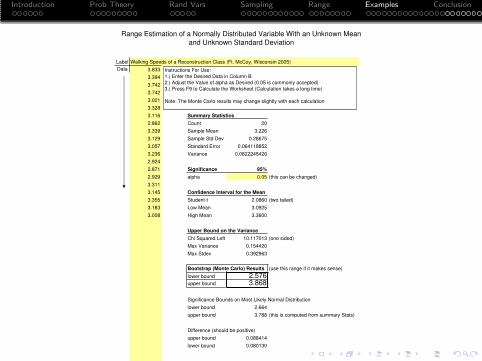
Label Walking Speeds of a Reconstruction Class (Ft. McCoy, Wisconsin 2005)
Data 3.833
3.394
3.742
3.742
3.021
3.328
3.116 Summary Statistics
2.862 Count 20
3.339 Sample Mean 3.226
3.129 Sample Std Dev 0.28675
3.057 Standard Error 0.064118852
3.236 Variance 0.0822245426
2.924
2.871 Significance 95%
2.929 alpha 0.05 (this can be changed)
3.311
3.145 Confidence Interval for the Mean
3.355 Student-t 2.0860 (two tailed)
3.183 Low Mean 3.0925
3.008 High Mean 3.3600
Upper Bound on the Variance
Chi Squared Left 10.117013 (one sided)
Max Variance 0.154420
Max Stdev 0.392963
Bootstrap (Monte Carlo) Results (use this range if it makes sense)
lower bound 2.576upper bound 3.868
Significance Bounds on Most Likely Normal Distribution
lower bound 2.664
upper bound 3.788 (this is computed from summary Stats)
Difference (should be positive)
upper bound 0.088414
lower bound 0.080130
Instructions For Use:
1.) Enter the Desired Data in Column B
2.) Adjust the Value of alpha as Desired (0.05 is commonly accepted)
3.) Press F9 to Calculate the Worksheet (Calculation takes a long time)
Note: The Monte Carlo results may change slightly with each calculation

Introduction Prob Theory Rand Vars Sampling Range Examples Conclusion
Range Estimation of a Normally Distributed Variable With an Unknown Mean
and Unknown Standard Deviation
Label Walking Speeds of a Reconstruction Class (Ft. McCoy, Wisconsin 2005)
Data 3.833
3.394
3.742
3.742
3.021
3.328
3.116 Summary Statistics
2.862 Count 24
3.339 Sample Mean 3.249
3.129 Sample Std Dev 0.28621
3.057 Standard Error 0.058421803
3.236 Variance 0.0819145686
2.924
2.871 Significance 95%
2.929 alpha 0.05 (this can be changed)
3.311
3.145 Confidence Interval for the Mean
3.355 Student-t 2.0639 (two tailed)
3.183 Low Mean 3.1287
3.008 High Mean 3.3698
3.145
3.084 Upper Bound on the Variance
3.672 Chi Squared Left 13.090514 (one sided)
3.557 Max Variance 0.143924
Max Stdev 0.379373
Bootstrap (Monte Carlo) Results (use this range if it makes sense)
lower bound 2.631upper bound 3.894
Significance Bounds on Most Likely Normal Distribution
lower bound 2.688
upper bound 3.810 (this is computed from summary Stats)
Difference (should be positive)
upper bound 0.057733
lower bound 0.083869
Instructions For Use:
1.) Enter the Desired Data in Column B
2.) Adjust the Value of alpha as Desired (0.05 is commonly accepted)
3.) Press F9 to Calculate the Worksheet (Calculation takes a long time)
Note: The Monte Carlo results may change slightly with each calculation

Introduction Prob Theory Rand Vars Sampling Range Examples Conclusion
Range Estimation of a Normally Distributed Variable With an Unknown Mean
and Unknown Standard Deviation
Label Walking Speeds of a Reconstruction Class (Ft. McCoy, Wisconsin 2005)
Data 3.833
3.394
3.742
3.742
3.021
3.328
3.116 Summary Statistics
2.862 Count 28
3.339 Sample Mean 3.277
3.129 Sample Std Dev 0.28717
3.057 Standard Error 0.054270051
3.236 Variance 0.0824666760
2.924
2.871 Significance 95%
2.929 alpha 0.05 (this can be changed)
3.311
3.145 Confidence Interval for the Mean
3.355 Student-t 2.0484 (two tailed)
3.183 Low Mean 3.1661
3.008 High Mean 3.3885
3.145
3.084 Upper Bound on the Variance
3.672 Chi Squared Left 16.151396 (one sided)
3.557 Max Variance 0.137858
3.242 Max Stdev 0.371292
3.212
3.568 Bootstrap (Monte Carlo) Results (use this range if it makes sense)
3.761 lower bound 2.670upper bound 3.908
Significance Bounds on Most Likely Normal Distribution
lower bound 2.714
upper bound 3.840 (this is computed from summary Stats)
Difference (should be positive)
upper bound 0.044502
lower bound 0.067699
Instructions For Use:
1.) Enter the Desired Data in Column B
2.) Adjust the Value of alpha as Desired (0.05 is commonly accepted)
3.) Press F9 to Calculate the Worksheet (Calculation takes a long time)
Note: The Monte Carlo results may change slightly with each calculation

Introduction Prob Theory Rand Vars Sampling Range Examples Conclusion
The Bounds on Walking Speeds According to the Number of
Samples
1
1.5
2
2.5
3
3.5
4
4.5
5
5.5
6
0 4 8 12 16 20 24 28
Number of Samples
Wa
lkin
g S
pe
ed
s (
mp
h)
Upper Bound
MLE Upper Bound
Mean
MLE Lower Bound
Lower Bound

Introduction Prob Theory Rand Vars Sampling Range Examples Conclusion
Sample Size Effect
As the number of samples increases, we recover the inherentvariability.
With small samples we are more uncertain the fixed butunknown parameters.
More samples reduces the difference between ”most likely”and Bootstrap Method.
Walking speeds follow a normal distribution.

Introduction Prob Theory Rand Vars Sampling Range Examples Conclusion
Graph Showing the Effect of Sample Size
Cumulative Probability of Walking Speeds
0
0.1
0.2
0.3
0.4
0.5
0.6
0.7
0.8
0.9
1
2.50 3.00 3.50 4.00
Walking Speed (mph)
Cu
mu
lati
ve P
rob
ab
ilit
y
Emperical
Normal

Introduction Prob Theory Rand Vars Sampling Range Examples Conclusion
Variation Between Drag Sleds and Accelerometers
Example
Determine the range from a series of friction tests based from dragsleds and accelerometers.
Friction determination of the same surface at the same timeusing different techniques
NAPARS Conference June of 2005 in Columbus OH
Vehicle mounted accelerometer (VC3000)
Friction based on drag sleds
Determine a range given both sets of data

Introduction Prob Theory Rand Vars Sampling Range Examples Conclusion
Range Estimation of a Normally Distributed Variable With an Unkown Mean and
Unknown Standard Deviation
Label Drag Factor NAPARS VC3000
Data 0.640
0.645
0.625
0.661
0.645
0.645
0.608 Summary Statistics
0.599 Count 15
0.677 Sample Mean 0.644
0.645 Sample Std Dev 0.02851
0.645 Standard Error 0.00736
0.645 Variance 0.00081
0.626
0.630 Confidence 95%
0.720 alpha 0.05 (this can be changed)
Confidence Interval for the Mean
Student-t 2.1314 (two tailed)
Low Mean 0.6280
High Mean 0.6594
Upper Bound on the Variance
Chi Squared Left 6.5706 (one sided)
Max Variance 0.00173
Max Stdev 0.04161
Monte Carlo Results (use this range if it makes sense)
lower bound 0.576upper bound 0.710
Confidence Bounds on Most Likely Normal Distribution
lower bound 0.588
upper bound 0.700 (this is computed from summary Stats)
Difference (should be positive)
upper bound 0.011949
lower bound 0.010764
Instructions For Use:
1.) Enter the Desired Data in Column B
2.) Adjust the Value of alpha as Desired (0.05 is commonly accepted)
3.) Press F9 to Calculate the Worksheet (Calculation takes a long time)
Note: The Monte Carlo results may change slightly with each calculation

Introduction Prob Theory Rand Vars Sampling Range Examples Conclusion
Range Estimation of a Normally Distributed Variable With an Unkown Mean and
Unknown Standard Deviation
Label Drag Factor NAPARS Drag Sled
Data 0.736
0.670
0.736
0.730
0.730
0.730
0.736 Summary Statistics
0.800 Count 21
0.736 Sample Mean 0.703
0.676 Sample Std Dev 0.10572
0.860 Standard Error 0.02307
0.500 Variance 0.01118
0.550
0.500 Confidence 95%
0.550 alpha 0.05 (this can be changed)
0.736
0.736 Confidence Interval for the Mean
0.736 Student-t 2.0796 (two tailed)
0.730 Low Mean 0.6555
0.920 High Mean 0.7515
0.675
Upper Bound on the Variance
Chi Squared Left 10.8508 (one sided)
Max Variance 0.02060
Max Stdev 0.14352
Monte Carlo Results (use this range if it makes sense)
lower bound 0.464upper bound 0.943
Confidence Bounds on Most Likely Normal Distribution
lower bound 0.496
upper bound 0.911 (this is computed from summary Stats)
Difference (should be positive)
upper bound 0.032682
lower bound 0.031892
Instructions For Use:
1.) Enter the Desired Data in Column B
2.) Adjust the Value of alpha as Desired (0.05 is commonly accepted)
3.) Press F9 to Calculate the Worksheet (Calculation takes a long time)
Note: The Monte Carlo results may change slightly with each calculation

Introduction Prob Theory Rand Vars Sampling Range Examples Conclusion
Drag Sled and Accelerometer Remarks
The range from the accelerometer was 0.57 to 0.71
The range from the drag sleds was was 0.46 to 0.94
This was the same surface– different techniques!
More consistent testing methods reduce variation.
Make sure the samples come from the same population.
Make sure the population represents the proper physics.
The probability of getting values in the tails is smaller thangetting a centrally located value.
Introduction Prob Theory Rand Vars Sampling Range Examples Conclusion
Outline
1 IntroductionMotivationStatistical Definitions
2 Probability TheoryAxioms of ProbabilityConditional ProbabilityBayes’ Theorem
3 Random VariablesNormal DistributionCentral Limit Theorem
4 SamplingDescriptive Statistics
Statistics for the MeanStatistics for the Variance
5 Determining a RangeFrequentist AssumptionsSignificance levelsThe Bootstrapping Method
6 ExamplesDrag FactorsCrush Stiffness CoefficientsPerception-Reaction TimeWalking SpeedsDrag Sleds vs. Accelerometers
7 Conclusion

Introduction Prob Theory Rand Vars Sampling Range Examples Conclusion
Conclusions
If the parent population is near normally distributed, then arange can be determined based on sampling statistics.
As the number of samples increases, the unknown populationmean and standard deviation will converge to the estimatedmean and standard deviation.
If an underlying distribution is clearly not normal, then therange obtained herein may be inappropriate.
The distribution of the mean always follows a Student-tdistribution.
If the population is normally distributed and the range seemtoo large, then more samples must be obtained.
This technique does not acknowledge any prior understandingof the data.

Introduction Prob Theory Rand Vars Sampling Range Examples Conclusion
References I
B. M. Ayyub and R. H. McCuen.Probability, Statistics, and Reliability for Engineers.CRC Press LLC, Boca Raton, 1997.
Colin G. G. Aitken and Franco Taroni.Statistics and the Evaluation of Evidence for ForensicScientists.John Wiley & Sons, Chichester, 2004.
W. Bartlett et al.Evaluating the uncertianty in various measurement taskscommon to accident reconstruction.In Accident Reconstruction SP-1666, number 2002-01-0546 inSP, pages 57–70. Society of Automotive Engineers,Warrendale, PA, March 2002.

Introduction Prob Theory Rand Vars Sampling Range Examples Conclusion
References II
R. B. Dean and W. J. Dixon.Simplified statistics for small numbers of observations.Analytical Chemistry, 23(4):636–638, 1951.
Larry Gonick and Woollcott Smith.The Cartoon Guide To Statistics.Harper Collins, New York, 1993.A good introduction to statistics.
James Joyce.Bayes’ theorem.In Ed-ward N. Zalta, editor, The Stanford Encyclopedia of Philosophy.http://plato.stanford.edu/archives/win2003/entries/bayes-
Winter 2003.Last accessed on 17 August 2005.

Introduction Prob Theory Rand Vars Sampling Range Examples Conclusion
References III
C. C. O. Marks.Accident analysis uncertianty in the forensic context.Personal Communication, 2002.
Jeffrey W. Muttart, William F. Messerschmidt, and Larry G.Gillen.Relationship between relative velocity detection and driverresponse time in vehicle following situations.In Human Factors in Driving, Telematics and Seating Comfort(SP-1934), number 2005-01-0427. Society of AutomotiveEngineers, Warrendale, PA, 2005.

Introduction Prob Theory Rand Vars Sampling Range Examples Conclusion
References IV
Douglas C. Montgomery.Design and Analysis of Experiments.John Wiley and Sons, New York, 5th edition, 2004.A complete discussion of designing, conducting, and analyzingexperiments.
William L. Oberkampf, Jon C. Helton, and Kari Sentz.Mathematical representation of uncertainty.American Institute of Aeronautics and Astronautics (AIAA),(1645):1–22, 2001.
Bernard Roberson and G. A. Vignaux.Interpreting Evidence: Evaluating Foresic Science in theCourtroom.John Wiley & Sons, Chichester, 1995.

Introduction Prob Theory Rand Vars Sampling Range Examples Conclusion
References V
Rinaldo B. Schinazi.Probability with Statistical Applications.Birkhauser, Boston, 2001.
Daniel W. Vomhof.A comprehensible approach to statistical evaluation indocument examination.Personal Communication, 2002.
Pete Wildman.Estimating a population standard deviation or variance.http://wind.cc.whecn.edu/~pwildman/statnew/estimating_a_population_standard_devation_or_varia
2002.Last accessed on 28 August 2005.