finding hyperbolic structures of and surfaces in 3–manifolds
TRANSCRIPT

Varieties associated to 3–manifolds:
Finding Hyperbolic Structures of
and Surfaces in 3–Manifolds
August 2003
Stephan Tillmann
1

2 Contents
Contents
1. Geometry and Surfaces 3
2. From Surfaces to Actions on Trees 11
3. From Actions on Trees to Surfaces 18
4. The Varieties 29
5. Surfaces and Ideal Points 45
6. The Weak Neuwirth Conjecture 51
7. Boundary slopes and the A–polynomial 55
8. Representations and the Alexander polynomial 62
9. The Roots of Unity Phenomenon 67
10. Detected surfaces 74
References 81
These notes were compiled for a short course given at the University of Mel-
bourne, 5-8 February 2001, and much of the material has been taken from or is
based on the following references:
(1) W.D. Neumann: Notes on Geometry and 3–Manifolds [23].
(2) G. Baumslag: Topics in Combinatorial Group Theory [2].
(3) P.B. Shalen: Representations of 3–manifold groups [27].
(4) D. Cooper, M. Culler, H. Gillett, D.D. Long, P.B. Shalen: Plane curves
associated to character varieties of 3–manifolds [7].
This compilation is intended as a hands–on guide to the computation of character
varieties and A–polynomials, as well as an exposition to the construction by Culler
and Shalen which associates essential surfaces to ideal points of curves in the afore-
mentioned algebraic varieties. It is also described how one can decide whether a
connected essential surface is associated to an ideal point, thus providing a tool
useful in the study of examples.
section 1 3
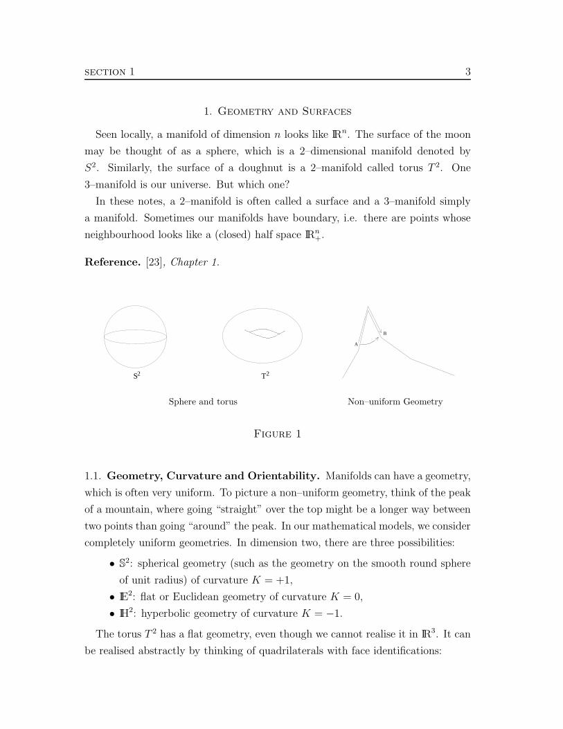
1. Geometry and Surfaces
Seen locally, a manifold of dimension n looks like IRn. The surface of the moon
may be thought of as a sphere, which is a 2–dimensional manifold denoted by
S2. Similarly, the surface of a doughnut is a 2–manifold called torus T 2. One
3–manifold is our universe. But which one?
In these notes, a 2–manifold is often called a surface and a 3–manifold simply
a manifold. Sometimes our manifolds have boundary, i.e. there are points whose
neighbourhood looks like a (closed) half space IRn+.
Reference. [23], Chapter 1.
S2 T2
Sphere and torus
A
B
Non–uniform Geometry
Figure 1
1.1. Geometry, Curvature and Orientability. Manifolds can have a geometry,
which is often very uniform. To picture a non–uniform geometry, think of the peak
of a mountain, where going “straight” over the top might be a longer way between
two points than going “around” the peak. In our mathematical models, we consider
completely uniform geometries. In dimension two, there are three possibilities:
• S2: spherical geometry (such as the geometry on the smooth round sphere
of unit radius) of curvature K = +1,
• IE2: flat or Euclidean geometry of curvature K = 0,
• IH2: hyperbolic geometry of curvature K = −1.
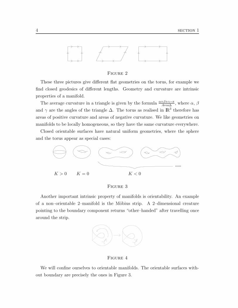
The torus T 2 has a flat geometry, even though we cannot realise it in IR3. It can
be realised abstractly by thinking of quadrilaterals with face identifications:
4 section 1
Figure 2
These three pictures give different flat geometries on the torus, for example we
find closed geodesics of different lengths. Geometry and curvature are intrinsic
properties of a manifold.
The average curvature in a triangle is given by the formula α+β+γ−π
Area∆, where α, β
and γ are the angles of the triangle ∆. The torus as realised in IR3 therefore has
areas of positive curvature and areas of negative curvature. We like geometries on
manifolds to be locally homogeneous, so they have the same curvature everywhere.
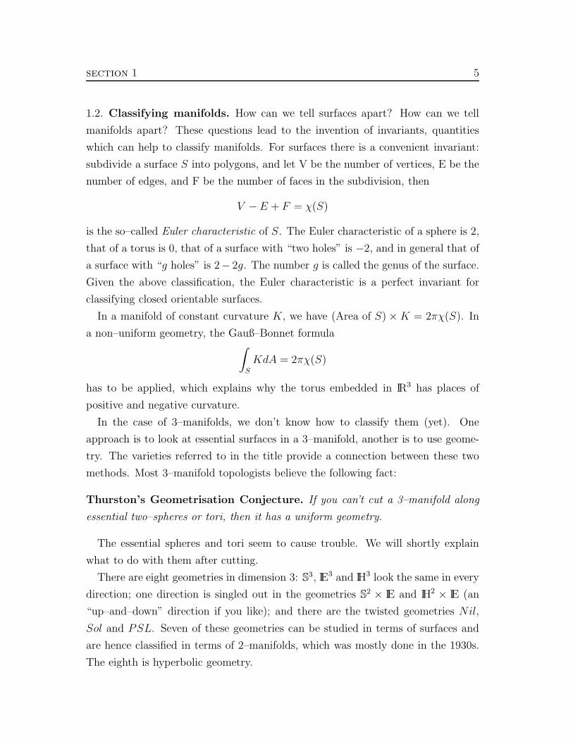
Closed orientable surfaces have natural uniform geometries, where the sphere
and the torus appear as special cases:
.....
K > 0 K = 0 K < 0
Figure 3
Another important intrinsic property of manifolds is orientability. An example
of a non–orientable 2–manifold is the Mobius strip. A 2–dimensional creature
pointing to the boundary component returns “other–handed” after travelling once
around the strip.
Figure 4
We will confine ourselves to orientable manifolds. The orientable surfaces with-
out boundary are precisely the ones in Figure 3.
section 1 5
1.2. Classifying manifolds. How can we tell surfaces apart? How can we tell
manifolds apart? These questions lead to the invention of invariants, quantities
which can help to classify manifolds. For surfaces there is a convenient invariant:
subdivide a surface S into polygons, and let V be the number of vertices, E be the
number of edges, and F be the number of faces in the subdivision, then
V −E + F = χ(S)
is the so–called Euler characteristic of S. The Euler characteristic of a sphere is 2,
that of a torus is 0, that of a surface with “two holes” is −2, and in general that of
a surface with “g holes” is 2− 2g. The number g is called the genus of the surface.
Given the above classification, the Euler characteristic is a perfect invariant for
classifying closed orientable surfaces.
In a manifold of constant curvature K, we have (Area of S) ×K = 2πχ(S). In
a non–uniform geometry, the Gauß–Bonnet formula∫
S
KdA = 2πχ(S)
has to be applied, which explains why the torus embedded in IR3 has places of
positive and negative curvature.
In the case of 3–manifolds, we don’t know how to classify them (yet). One
approach is to look at essential surfaces in a 3–manifold, another is to use geome-
try. The varieties referred to in the title provide a connection between these two
methods. Most 3–manifold topologists believe the following fact:
Thurston’s Geometrisation Conjecture. If you can’t cut a 3–manifold along
essential two–spheres or tori, then it has a uniform geometry.
The essential spheres and tori seem to cause trouble. We will shortly explain
what to do with them after cutting.
There are eight geometries in dimension 3: S3, IE3 and IH3 look the same in every
direction; one direction is singled out in the geometries S2 × IE and IH2 × IE (an
“up–and–down” direction if you like); and there are the twisted geometries Nil,
Sol and PSL. Seven of these geometries can be studied in terms of surfaces and
are hence classified in terms of 2–manifolds, which was mostly done in the 1930s.
The eighth is hyperbolic geometry.

6 section 1
1.3. Hyperbolic Geometry. How can we understand hyperbolic geometry? We
change from the geometry to a mathematical model. An example is the upper half
space model:
C × IR+ = {(z, r) | z = x+ iy, r > 0},
where a measure for arc length is given by taking the Euclidean measure
ds =√
dx2 + dy2 + dr2
and dividing by the height:
dshyp =1
rds =
1
r
√
dx2 + dy2 + dr2.
Hyperbolic planes are hemispheres, and we have a concept of points at infinity,
which lie on the Riemann sphere C ∪ {∞}. A nice feature of hyperbolic geometry
is that infinite objects can have finite volume, such as ideal tetrahedra.
α
Euclidean angle
Straight lines
Upper half space model Ideal tetrahedron
Figure 5
Consider again the flat torus. A 2–dimensional creature living on the torus
(with a particular flat geometry) must feel like living in the plane where things are
copied and move in parallel lines as shown in Figure 6. The group of motions Γ
takes a fundamental domain into another copy, and is a subgroup of Isom(IE2).
The given torus is obtained as T 2 = IE2/Γ. This picture works for any geometry
and dimension:
Definition 1. [23] A geometric manifold (or manifold with a geometric structure)
is a manifold of finite volume of the form X/Γ, where X is a geometry and Γ is a
discrete subgroup of the isometry group Isom(X).

section 1 7
Figure 6
When we are interested in orientable hyperbolic 3–manifolds, we are interested
in M = IH3/Γ, where Γ is a discrete subgroup of
Isom+(IH3) ∼= PSL2(C) = {(
a b
c d
)
| ad− bc = 1}/{±(
1 0
0 1
)
}.
An element in the orientation preserving isometry group is determined by how
points at infinity get moved:(
a b
c d
)
z =az + b
cz + d.
A hyperbolic structure on a 3–manifold M is a complete Riemannian metric of
constant sectional curvature −1. If M admits such a structure, its universal cover
is isometrically identified with hyperbolic 3–space IH3. If M is orientable, the action
of π1(M) by deck transformations on IH3 defines a representation of π1(M) into
Isom+IH3 ∼= PSL2(C).
1.4. Decomposing manifolds. Following Thurston’s Geometrisation Conjecture,
we cut a given manifold along essential spheres and tori. We then take a connected
component which results from this process, fill in the spheres with balls and add
“tori at infinity” to obtain the so–called ends of the manifold.
Figure 7. End of a hyperbolic manifold
8 section 1
Adding “tori at infinity” is the same as taking the interior of a manifold with
boundary. Hyperbolic manifolds have no boundary; however, we may reverse the
above process to obtain compact cores (which have isomorphic fundamental groups)
and may talk about the boundary thereof.
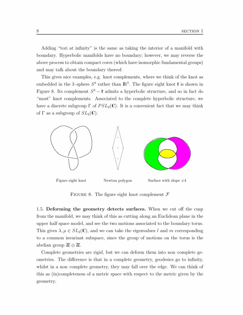
This gives nice examples, e.g. knot complements, where we think of the knot as
embedded in the 3–sphere S3 rather than IR3. The figure eight knot k is shown in
Figure 8. Its complement S3 − k admits a hyperbolic structure, and so in fact do
“most” knot complements. Associated to the complete hyperbolic structure, we
have a discrete subgroup Γ of PSL2(C). It is a convenient fact that we may think
of Γ as a subgroup of SL2(C).
Figure eight knot Newton polygon Surface with slope ±4
Figure 8. The figure eight knot complement F
1.5. Deforming the geometry detects surfaces. When we cut off the cusp
from the manifold, we may think of this as cutting along an Euclidean plane in the
upper half space model, and see the two motions associated to the boundary torus.
This gives λ, µ ∈ SL2(C), and we can take the eigenvalues l and m corresponding
to a common invariant subspace, since the group of motions on the torus is the
abelian group ZZ ⊕ ZZ.
Complete geometries are rigid, but we can deform them into non–complete ge-
ometries. The difference is that in a complete geometry, geodesics go to infinity,
whilst in a non–complete geometry, they may fall over the edge. We can think of
this as (in)completeness of a metric space with respect to the metric given by the
geometry.
section 1 9
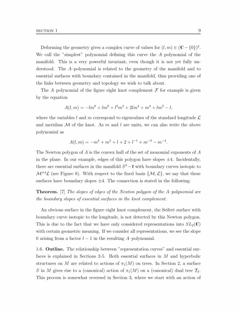
Deforming the geometry gives a complex curve of values for (l,m) ∈ (C−{0})2.
We call the ”simplest” polynomial defining this curve the A–polynomial of the
manifold. This is a very powerful invariant, even though it is not yet fully un-
derstood. The A–polynomial is related to the geometry of the manifold and to
essential surfaces with boundary contained in the manifold, thus providing one of
the links between geometry and topology we wish to talk about.
The A–polynomial of the figure eight knot complement F for example is given
by the equation
A(l,m) = −lm8 + lm6 + l2m4 + 2lm4 +m4 + lm2 − l,
where the variables l and m correspond to eigenvalues of the standard longitude Land meridian M of the knot. As m and l are units, we can also write the above
polynomial as
A(l,m) = −m4 +m2 + l + 2 + l−1 +m−2 −m−4.
The Newton polygon of A is the convex hull of the set of monomial exponents of A
in the plane. In our example, edges of this polygon have slopes ±4. Incidentally,
there are essential surfaces in the manifold S3 − k with boundary curves isotopic to
M±4L (see Figure 8). With respect to the fixed basis {M,L}, we say that these
surfaces have boundary slopes ±4. The connection is stated in the following:
Theorem. [7] The slopes of edges of the Newton polygon of the A–polynomial are
the boundary slopes of essential surfaces in the knot complement.
An obvious surface in the figure eight knot complement, the Seifert surface with
boundary curve isotopic to the longitude, is not detected by this Newton polygon.
This is due to the fact that we have only considered representations into SL2(C)
with certain geometric meaning. If we consider all representations, we see the slope
0 arising from a factor l − 1 in the resulting A–polynomial.
1.6. Outline. The relationship between ”representation curves” and essential sur-
faces is explained in Sections 2-5. Both essential surfaces in M and hyperbolic
structures on M are related to actions of π1(M) on trees. In Section 2, a surface
S in M gives rise to a (canonical) action of π1(M) on a (canonical) dual tree TS.
This process is somewhat reversed in Section 3, where we start with an action of

10 section 1
π1(M) on a tree T and then construct an associated surface S in M . However, an
associated surface S is not canonical, and we will compare the action on T which
we started from to the action on the dual tree TS. This leads to some first ap-
plications, and we will also characterise surfaces that can be associated to a given
action.
The representation and character varieties are defined and explored a little in
Section 4, and the construction by Culler and Shalen is completed in Section 5 by
associating an action on a tree to an ideal point of a representation curve.
In the remaining five sections, various applications are given. We first prove
the Weak Neuwirth Conjecture in Section 6, whose proof leads to information
about boundary slopes of associated surfaces, and hence to the above mentioned
”boundary slopes” theorem in Section 7, where we define the A–polynomial. The
material on roots of the Alexander polynomial and eigenvalues of metabelian rep-
resentations in Section 8 does not use Culler–Shalen theory, and can readily be
understood with little knowledge about representations. However, it fits into the
general theme of trying to give representations geometric meaning. In the last two
sections, more information about associated surfaces is gained, which leads to the
roots of unity phenomenon and necessary and sufficient conditions on connected
associated surfaces.
Acknowledgements. The introduction is inspired by a lecture Walter Neumann
gave at Columbia University on 5 June 2000. The material on Culler–Shalen theory
is mostly taken from Shalen [27]. Some of the original material contained in these
notes now forms part of [32, 33].
Much of the contents had been covered in a working seminar at Columbia Uni-
versity, in which Abhijit Champanerkar, Brian Mangum, Walter Neumann and
Stephan Tillmann lectured. I would like to thank these co–lecturers, as well as
Radu Popescu and the other participants of this seminar. Furthermore, I would
like to thank Craig Hodgson for helpful conversations.
section 2 11
2. From Surfaces to Actions on Trees
This section reviews some material on groups acting on trees, defines essential
surfaces in 3–manifolds, and gives some flavour of the interplay between topology
and algebra.
Reference. [27], Section 1.
2.1. Group actions. An action of a group Γ on a setX is a function · : Γ×X → X
that satisfies 1 ·x = x and (γδ) ·x = γ ·(δ ·x) for all x ∈ X and all elements γ, δ ∈ Γ.
An action gives a partition of the set X into orbits. Two elements x, y ∈ X are
contained in the same orbit if and only if there is an element γ ∈ Γ such that
γ · x = y. We denote the orbit of x by Γ · x. The stabilizer Γx of x ∈ X is the
collection of all elements in Γ such that γ · x = x.
Exercise 1. Show that the stabilizer of x ∈ X is a subgroup of Γ, and that for each
x ∈ X the map Γ → X defined by γ → γ · x induces a bijection between the set of
cosets γΓx and the orbit Γ · x of x.
We call an action free if the stabiliser of every element ofX is the trivial subgroup
of X. A subset S ⊆ X is invariant under the action if γ · s ∈ S for each s ∈ S and
for each γ ∈ Γ. That is, S is a union of orbits. An element is fixed by Γ if {x} is
invariant.
Suppose the group Γ acts on two sets X and Y in the ways · and • respectively.
A map f : X → Y is said to be Γ–equivariant if
f(γ · x) = γ • f(x) ∀x ∈ X ∀γ ∈ Γ.
An action that will appear in the sequel is the action of the fundamental group
of a 3–manifold M on its universal covering space (M, p) by deck transformations.
By the uniqueness of the universal cover, we may suppress base points, since even
though π1(M,x) operates on p−1(x), we have π1(M,x) ∼= Aut(M, p), which is
defined up to equivalence. If M is given a triangulation, then M inherits a trian-
gulation such that the action of π1(M) on M is simplicial. This will be important
later, and we will not distinguish between the simplicial complex and its topological
realisation.

12 section 2
Exercise 2. Starting with a triangulation of M , give M an induced triangulation
such that the covering projection is a simplicial map.
2.2. Graphs and trees. A graph G consists of a non–empty set of vertices V =
V(G) and a set of edges E = E(G), together with the three maps
i : E → V, t : E → V, − : E → E ,
subject to the condition that if e ∈ E , then
e 6= e and e = e.
Thus, the third map is a fixed point free involution on the set of edges, and cor-
responds to reversal of orientation. The second condition implies that t(e) = i(e).
We call e the inverse of e, and t(e) the terminal and i(e) the initial vertex. They
are the extremities of an edge, and we call two vertices adjacent if they are the
extremities of some edge. If i(e) = t(e), then e is called a loop.
When we draw diagrams of graphs, we omit one of e and its inverse, and indicate
orientation by an arrow pointing towards the terminus. The simplest example of a
graph is a point.
A group Γ acts on a graph if it comes equipped with a homomorphism ϕ : Γ →Aut(G), where Aut(G) consists of invertible morphisms G → G with composition
as the binary operation. We denote the image of a vertex v under the action of
γ ∈ Γ by γ · v. A group acts on a graph without inversions if γ · e 6= e for all e ∈ Eand for all γ ∈ Γ. We say that the action is trivial if a vertex of G is fixed by Γ.
Exercise 3. What is the automorphism group of the following graph?
Example. A group acts on its Cayley graph by left multiplication. To construct
the Cayley graph, take Γ as the set of vertices, and for a fixed generating set S we
get the set of edges from the disjoint union of Γ×S and S×Γ. The three functions
are defined by i(γ, s) = γ, t(γ, s) = γs, (γ, s) = (s, γ) and (s, γ) = (γ, s).

section 2 13
Exercise 4. What is the Cayley graph of the trivial group, a finite cyclic group,
an infinite cyclic group?
A path of length n in G is a sequence e1, . . . , en of edges such that i(ei) = t(ei−1)
for i = 2, . . . , n. The vertices i(e1) and t(en) are the extremities of the path. A
path is closed if i(e1) = t(en). A pair ei, ei+1 is termed a backtracking if ei+1 = ei.
A graph G is connected if any two vertices are the extremities of some path, and
it is a tree if it is connected and every closed path of positive length in G contains
a backtracking.
Exercise 5. (1) A group acts on its Cayley graph without inversions.
(2) The Cayley graph is connected.
(3) The Cayley graph contains a loop if and only if 1 ∈ S.
If a group Γ acts without inversions on a graph G, the orbit space G/Γ inherits
the structure of a graph as follows. Denote the orbits of edges and vertices by [·].We have edges [e] = Γ · e, and now define the functions by
i[e] = [i(e)], t[e] = [t(e)], [e] = [e].
Note that the inversion function is fixed point free and of order two since Γ acts
without inversions. Then the quotient map G → G/Γ defined by e → [e] and
v → [v] is a morphism of graphs.
Let Γ be a group acting on a tree T . The translation length of an element is
defined by
`(γ) = min{d(v, γ · v) | v ∈ T }.Group elements which fix a vertex have translation length equal to zero, and are
called elliptic. The set of fixed points of an elliptic element is a subtree of T . An
element with positive translation length is called loxodromic. Loxodromic elements
act by translations along a unique line, which is called their axis, and denoted by
A(γ). The invariant set of an element γ is understood to be its fixed set if it is
elliptic and its axis if it is loxodromic.
Lemma 2. [25] Let Γ be a finitely generated group which acts simplicially on a
tree. Let the generators of Γ be γ1, . . ., γm, and assume that γi and γiγj have fixed
points for all i, j. Then Γ fixes a vertex.
14 section 2
Exercise 6. Prove the lemma!
2.3. Essential surfaces. A surface S in a compact 3–manifold M will always
mean a 2–dimensional PL submanifold properly embedded in M , that is, a closed
subset of M with ∂S = S ∩ ∂M . If M is not compact, we replace it by a compact
core. An embedded sphere S2 in a 3–manifold M is called incompressible if it does
not bound an embedded ball in M , and a 3–manifold is irreducible if it contains
no incompressible 2–spheres.
An orientable surface S without 2–sphere or disc components in an orientable
3–manifold M is called irreducible if for each disc D ⊂M with D ∩ S = ∂D there
is a disc D′ ⊂ S with ∂D′ = ∂D. We will also use the following definition:
Definition 3. [27] A surface S in a compact, irreducible, orientable 3–manifold is
said to be essential if it has the following five properties:
(1) S is bicollared;
(2) the inclusion homomorphism π1(Si) → π1(M) is injective for every compo-
nent Si of S;
(3) no component of S is a 2–sphere;
(4) no component of S is boundary parallel;
(5) S is non-empty.
A bicollaring of a surface S in M is a homeomorphism h : S× [−1, 1] →M such
that h(x, 0) = x for every x ∈ S and
h(∂S × [−1, 1]) = ∂M ∩ h(S × [−1, 1]).
The existence of a bicollaring implies that the surface is 2–sided, i.e. that S sepa-
rates any sufficiently small neighbourhood of itself in M . For surfaces in orientable
manifolds, 2–sidedness is equivalent to orientability.
The second condition in the above definition is equivalent to saying that there
are no compression discs for the surface (cf. [19], Lemma 6.1). A compression disc
is an embedded disc in M such that its boundary lies on S and is not contractible
on S. If there is such a disc, then the second property clearly fails. Conversely,
if the second property fails, then there is a non–trivial simple closed curve on S
which is contractible in M . Using the bicollaring, we obtain an embedded annulus
section 2 15
which bounds a possibly immersed disc in M . Dehn’s lemma yields that there is
an embedded disc with the same boundary curve.
� �� �� �� �� �� �� �� �� �� �� �� �� �
� �� �� �� �� �� �� �� �� �� �� �� �� �
� �� �� �� �� �� �� �� �� �� �� �� �� �
� �� �� �� �� �� �� �� �� �� �� �� �� �
� �� �� �� �� �� �� �� �� �� �� �
� �� �� �� �� �� �� �� �� �� �� �
� �� �� �� �� �� �� �
� �� �� �� �� �� �� �
� � �� � �� � �� � �� � �� � �� � �
� � �� � �� � �� � �� � �� � �� � �
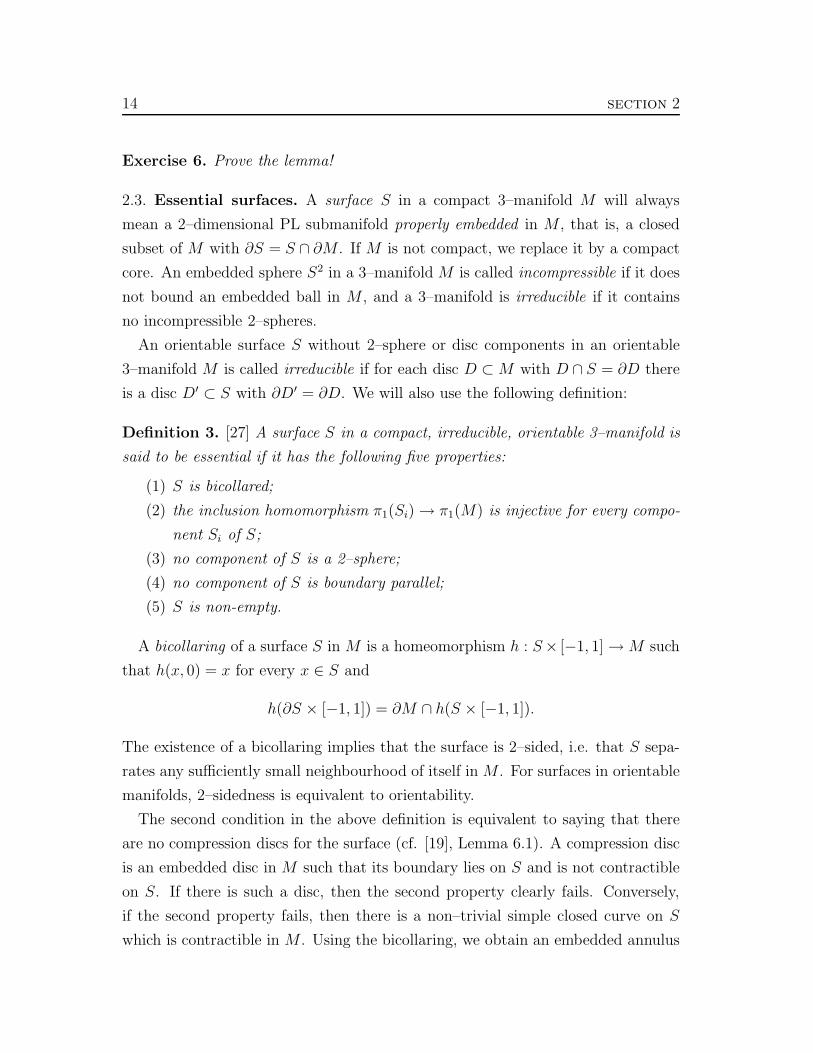
Figure 9. Compressions of a surface
If a surface admits a compression disc, we may cut the surface along the boundary
of this disc and close the resulting “holes” in our surface with two discs. We call
this process a compression of the surface. Two compressions of a genus two surface
are shown in Figure 9 – the separating compression results in two tori, whilst the
non–separating yields a single torus. The resulting surface tends to be simpler in
a sense which we will formalise later.
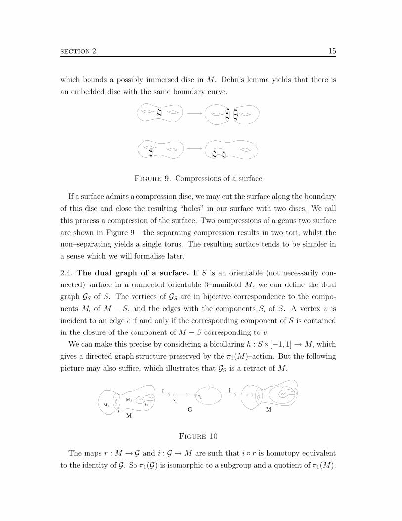
2.4. The dual graph of a surface. If S is an orientable (not necessarily con-
nected) surface in a connected orientable 3–manifold M , we can define the dual
graph GS of S. The vertices of GS are in bijective correspondence to the compo-
nents Mi of M − S, and the edges with the components Si of S. A vertex v is
incident to an edge e if and only if the corresponding component of S is contained
in the closure of the component of M − S corresponding to v.
We can make this precise by considering a bicollaring h : S× [−1, 1] → M , which
gives a directed graph structure preserved by the π1(M)–action. But the following
picture may also suffice, which illustrates that GS is a retract of M .
MM
MG
1
2
s
s
1
2
vv
12
ir
M
Figure 10
The maps r : M → G and i : G → M are such that i ◦ r is homotopy equivalent
to the identity of G. So π1(G) is isomorphic to a subgroup and a quotient of π1(M).
16 section 2
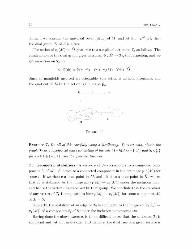
Thus, if we consider the universal cover (M, p) of M , and let S := p−1(S), then
the dual graph TS of S is a tree.
The action of π1(M) on M gives rise to a simplicial action on TS as follows. The
construction of the dual graph gives us a map Φ : M → TS, the retraction, and we
get an action on TS by
γ · Φ(m) = Φ(γ · m) ∀γ ∈ π1(M) ∀m ∈ M.
Since all manifolds involved are orientable, this action is without inversions, and
the quotient of TS by the action is the graph GS.
M
MM
MG
1
2
s
s
1
2
vv
12
T
φ
Φ
p
~
Figure 11
Exercise 7. Do all of this carefully using a bicollaring. To start with, obtain the
graph GS as a topological space consisting of the sets M−h(S×(−1, 1)) and Si×{t}for each t ∈ (−1, 1) with the quotient topology.
2.5. Geometric stabilisers. A vertex v of TS corresponds to a connected com-
ponent K of M − S, hence to a connected component in the preimage p−1(Mi) for
some i. If we choose a base point in Mi and lift it to a base point in K, we see
that K is stabilised by the image im(π1(Mi) → π1(M)) under the inclusion map,
and hence the vertex v is stabilised by that group. We conclude that the stabilizer
of any vertex of TS is conjugate to im(π1(Mi) → π1(M)) for some component Mi
of M − S.
Similarly, the stabilizer of an edge of TS is conjugate to the image im(π1(Si) →π1(M)) of a component Si of S under the inclusion homomorphism.
Having done the above exercise, it is not difficult to see that the action on TS is
simplicial and without inversions. Furthermore, the dual tree of a given surface is
section 2 17
well–defined up to simplicial equivalence since the bicollar is unique up to ambient
isotopy.
2.6. Non–trivial action. If the surface S is essential, the π1–injectivity condition
for components implies that for any component S0 of S a connected component
of p−1(S0) is a universal cover of S0. Applying Van Kampen’s theorem to the
fundamental group of M , it is not too hard to see that for any component Mi of
M − S the inclusion π1(Mi) → π1(M) is injective as well.
Recall that we term an action on a tree non–trivial, if no vertex of TS is fixed by
all of π1(M). We have the following
Proposition 4. Let S be an essential surface in a compact, connected, orientable,
irreducible 3–manifold M . Then the action of π1(M) on the dual tree TS is non–
trivial.
Proof. Assume that the action is trivial, so there is a vertex v such that Stab(v) =
π1(M). By our description of the stabilisers, this implies that there is a component
Mi of M − S such that the inclusion π1(Mi) → π1(M) is an isomorphism.
Since S is non–empty, there is a non–trivial component S0 of S. Since S0 is
not contained in Mi, there is a component M0 of M − S0 such that the inclusion
π1(M0) → π1(M) is surjective.
But if S0 does not separate M , this cannot be true since π1(M) would be a
HNN–extension of π1(M0) across π1(S0). So assume that S0 separates M . Then
there is another component M1 of M − S0. Since S0 is in the closure of both
components, there is an edge in the dual tree TS such that one vertex is stabilised
by π1(M0) = π1(M). Thus, any element which stabilises the other vertex has to
stabilise the whole edge. This implies that π1(M1) ∼= π1(S0). A theorem of Stallings
(see [19], Thm. 10.2) now implies that either M1 is the interior of a ball, hence
S0 = S2, or M1∼= (S0 × [0, 1]), which implies that S0 is boundary parallel. Either
case violates our choice of S. �
2.7. Splittings and graphs of groups. Review amalgamated products, HNN–
extensions and graphs of groups. Mention maximal tree and tree of representatives.
18 section 3
3. From Actions on Trees to Surfaces
We would now like to reverse the process described in the previous section. That
is, we would like to use a non–trivial simplicial action (without inversions) of the
fundamental group of a 3–manifold M on a tree T to construct an essential surface
in the manifold.
A surface dual to the action of π1(M) on a tree T is defined by Culler and Shalen
in [14] using a construction due to Stallings (see [27]). If the given manifoldM is not
compact, replace it by a compact core. Choose a triangulation of M and give the
universal cover M the induced triangulation, so that the fundamental group of M
acts simplicially on this induced triangulation. One can then construct a simplicial,
π1(M)–equivariant map f from M to T . The inverse image of midpoints of edges
is a surface in M which descends to a surface S in M . It turns out that since the
action of π1(M) on T is non–trivial, if necessary, one can change the map f by
homotopy such that the surface S is essential. The dual surface S depends upon
the choice of triangulation of M and the choice of the map f , and is therefore
not canonical. Furthermore, a dual surface often contains finitely many parallel
copies of some of its components. These parallel copies are somewhat redundant,
and we implicitly discard them, whilst we still call the resulting surface dual (or
associated) to the action.
Reference. [27], Section 2.
3.1. A π1(M)–equivariant map M → T . Suppose we have a simplicial action
of π1(M) on a tree T . We wish to construct a simplicial, π1(M)–equivariant map
f : M → T .
Fix a triangulation of M and give M the induced triangulation. We successively
construct maps f (i) from the i–skeleta M (i) of M to T such that each f (i) extends
f (i−1). In the process, we also successively create a subdivision of the triangulation
of M , which will remain π1(M)–invariant, and hence descend to a triangulation of
M .
To start, pick a set of orbit representatives S(0) for the action of π1(M) on the
set of vertices M (0). Let h(0) be any map from S(0) to the vertex set T (0) of T . We
claim that h(0) has exactly one π1(M)–equivariant extension f (0) : M (0) → T (0).

section 3 19
Indeed, uniqueness and existence follow from the condition
f (0)(γ · s) = γ · h(0)(s) ∀s ∈ S(0) ∀γ ∈ π1(M).
Note that this is well–defined since the action of π1(M) on M is free. So for every
vertex v in M (0) there are unique s and γ such that v = γ · s.Now then pick a set of orbit representatives S(1) for the action of π1(M) on the
set of all 1–simplices of M . For each edge σ ∈ S(1), the already constructed map
f (0) restricts to a map on the endpoints ∂σ. Since T is contractible, this map can
be extended to a continuous map hσ : σ → T , since there is a unique path in Tconnecting the images of the endpoints. Note that this map may not necessarily
be simplicial, since an edge in a triangulation of M could map to a path of length
n in the tree, but we may assume that hσ is linear.
Again, there is a unique, π1(M)–equivariant map f (1) : M (1) → T , which restricts
to hσ for each orbit representative σ, which must be given by
f (i+1)(γ · x) = γ · hσ(x) ∀s ∈ S(i+1) ∀x ∈ σ ∀γ ∈ π1(M).
As above, this map is well–defined and equivariant, and by construction continuous.
Since π1(M) acts simplicially on T , each edge contained in an orbit will map to
a path of the same length, say n, in T . In order to make f (1) simplicial, it is
well–defined and sufficient to subdivide the 1–skeleton accordingly by introducing
n−1 evenly spaced vertices on the elements of an orbit, which has a representative
mapped to a path of length n. Thus, f (1) : M (1) → T is π1(M)–equivariant and
simplicial.
We continue the process in the above manner: if f (i) has been constructed, then
pick a set of orbit representatives of the action of π1(M) on the initial set of (i+1)–
simplices, and for each representative σ, construct a continuous map hσ to T , which
agrees with f (i) on ∂σ. (Continuity again follows from the fact that T is simply
connected.) Now remember that we did introduce a subtriangulation of ∂σ and
use this to obtain a generalised barycentric subdivision of σ. Now make use of the
general simplicial approximation theorem:
General Simplicial Approximation Theorem (Munkres Thm 2.16.5). Let K
and L be complexes; let f : |K| → |L| be a continuous map. There exists a
subdivision K ′ of K such that f has a simplicial approximation h : K ′ → L.
20 section 3
Thus, we can take hσ to be this simplicial approximation, and give the (i+ 1)–
skeleton of M the induced triangulation which, by construction, is π1(M)–invariant.
In order to obtain a well–defined map f (i+1) : M (i+1) → T , we have to know that
hσ has not changed on the boundary of σ whilst we made the map simplicial. This
is guaranteed by the following
Lemma 5 (Spanier 3.4.1). Let f : |K| → |L| be a map and suppose that for some
subcomplex K1 ⊂ K, f ||K1| is induced by a simplicial map K1 → L. If ϕ : |K| → |L|is a simplicial approximation to f , then f ||K1| = ϕ||K1|.
So there is a unique, π1(M)–equivariant map f (i+1) : M (i+1) → T , which restrics
to hσ for each orbit representative σ. Again, this map must be given by
f (i+1)(γ · x) = γ · hσ(x) ∀s ∈ S(i+1) ∀x ∈ σ ∀γ ∈ π1(M).
As above, this map is well–defined, and by construction simplicial and π1(M)–
equivariant.
We finally obtain a simplicial, π1(M)–equivariant map f (3) : M → T , which we
denote by f , along with a new triangulation of M and M . We will freeze all these
objects until further notice.
Note that we have started with a given action and a given tree, but obtained f
by starting with any triangulation of M and any map h(0).
3.2. Constructing a dual surface. Consider a point x ∈ T which is not a vertex.
The inverse image f−1(x) = P is a subset of M , and we can look at its intersection
with a simplex σ of M .
If σ is a vertex, then clearly P ∩ σ = ∅. If f doesn’t map σ onto the edge e of Tcontaining x, then again P ∩ σ = ∅.
If f does map σ onto e, then P ∩ σ is an (i − 1)–cell properly embedded in σ
which misses the vertices. Embedded in affine space we may think of this as an
intersection of the simplex with a hyperplane. It follows that P is locally flat in
the interior of each tetrahedron of the triangulation. Is it also locally flat at the
intersections with 1–simplices?
Assume σ is such a 1–simplex and P ∩ σ = {z}. The 2–simplices incident to σ
look like the pages of a cyclic book with σ as its binding. The set P meets each
page in a 1–cell which has one endpoint at z and is otherwise disjoint from σ. Since
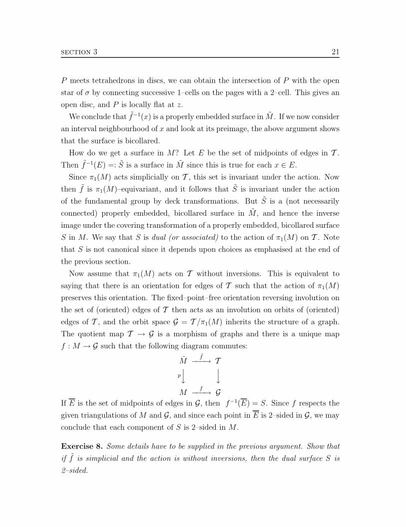
section 3 21
P meets tetrahedrons in discs, we can obtain the intersection of P with the open
star of σ by connecting successive 1–cells on the pages with a 2–cell. This gives an
open disc, and P is locally flat at z.
We conclude that f−1(x) is a properly embedded surface in M . If we now consider
an interval neighbourhood of x and look at its preimage, the above argument shows
that the surface is bicollared.
How do we get a surface in M? Let E be the set of midpoints of edges in T .
Then f−1(E) =: S is a surface in M since this is true for each x ∈ E.
Since π1(M) acts simplicially on T , this set is invariant under the action. Now
then f is π1(M)–equivariant, and it follows that S is invariant under the action
of the fundamental group by deck transformations. But S is a (not necessarily
connected) properly embedded, bicollared surface in M , and hence the inverse
image under the covering transformation of a properly embedded, bicollared surface
S in M . We say that S is dual (or associated) to the action of π1(M) on T . Note
that S is not canonical since it depends upon choices as emphasised at the end of
the previous section.
Now assume that π1(M) acts on T without inversions. This is equivalent to
saying that there is an orientation for edges of T such that the action of π1(M)
preserves this orientation. The fixed–point–free orientation reversing involution on
the set of (oriented) edges of T then acts as an involution on orbits of (oriented)
edges of T , and the orbit space G = T /π1(M) inherits the structure of a graph.
The quotient map T → G is a morphism of graphs and there is a unique map
f : M → G such that the following diagram commutes:
Mf−−−→ T
p
y
y
Mf−−−→ G
If E is the set of midpoints of edges in G, then f−1(E) = S. Since f respects the
given triangulations of M and G, and since each point in E is 2–sided in G, we may
conclude that each component of S is 2–sided in M .
Exercise 8. Some details have to be supplied in the previous argument. Show that
if f is simplicial and the action is without inversions, then the dual surface S is
2–sided.
22 section 3
Note that if M is orientable, 2–sidedness is equivalent to orientability of S. So
now we know that we get a locally flat, 2–sided, properly embedded, bicollared
surface. If we didn’t like things to be simplicial, we would have needed a property
which we got free in the simplicial setting: that f is transversal to the set of
midpoints.
3.3. Algebraic stabilisers. The vertex and edge stabilisers of the action have the
following properties:
Lemma 6. If S is a dual surface to an action of π1(M) on a tree T , then
• for each component Mi of M − S, the subgroup im(π1(Mi) → π1(M)) of
π1(M) is contained in the stabilizer of some vertex of T ; and
• for each component Si of S, the subgroup im(π1(Si) → π1(M)) of π1(M) is
contained in the stabilizer of some edge of T .
Exercise 9. Prove the lemma!
What if the surface associated to our action is empty? Then the only component
of M − S is M itself, and by the first part of the lemma, we know that π1(M)
stabilises a vertex of T . But this is what we called a trivial action. So if π1(M)
acts non–trivially on a tree, then every dual surface is non–empty.
3.4. Making the dual surface essential. Given a surface S dual to a non–
trivial, simplicial action without inversions on a tree, we know from the previous
section that it satisfies two of the five properties of essential surfaces. Can we
always choose a dual surface which is essential?
Let us assume that the dual surface S admits a compression disc D. We wish
to replace S by the surface S ′ resulting from compression along D such that S ′
is still dual to the action. So let us try to replace the map f by a map f ′ with
f ′−1(E) = p−1(S ′). We illustrate the process with a (simplified) picture in Figure
3.4. Continuity and π1(M)–equivariance are the easy properties to obtain, and our
picture is generic for their purpose, but simplicial is the crucial point.
Consider a ball neighbourhood B of the compression disc and pick a homeomor-
phic copy B of B in p−1(B). Our map f restricts to a map B → T , which we
will change on the interior of B. Inside our ball B, we have an annulus A and a

section 3 23
A
D DXX
f(A)
f(X )
f(X )
~ ~
~~
~
~
~
12
1
2
1~
= solid torus
= ball
B~
1 2
maps entirely to a vertex in T
since f is simplicial
(B-X )
Before: the map f restricted to B
� � � �� � � �� � � �� � � �� � � �� � � �� � � �� � � �� � � �� � � �� � � �
D D~ ~
~
1
2
B~
1 2 ZZ2 = ball
~2g(D )=g(D ) 1
g(Z )g(Z )
1
maps entirely to a vertex in T
= 2 balls
After: the map g restricted to B
Figure 12
compression disc D. Furthermore, there are two copies D1 and D2 of D such that
(D1 ∪ D2) ∩ ∂B = A ∩ ∂B.
The annulus A divides B into a ball X1 and a solid torus X2. Since A is 2–sided,
X1 is mapped into the closure of a different component of T −E than X2.
Note that the two discs D1 and D2 divide the ball B into three balls, and the
boundary of B into an annulus and two discs. The map f maps this annulus into
the image of X2, and the two discs into the image of X1. Thus, if we let Z2 be the
ball bounded by that annulus and the two discs D1 and D2, we have a continuous
24 section 3
map from its boundary to f(X2), which we can extend continuously to its interior
since all our objects are contractible.
Similarly, we have continuous maps from the boundaries of the other two balls
into the image of f(X1), which we can extend continuously to their interior. Call
the resulting map g : B → T . By the above construction, g agrees with f on the
boundary of B, and
g−1(f(B) ∩ E) = D1 ∪ D2S′ ∩ B.
In our illustration, g has also been obtained as a simplicial map. This is not easy
in general, but we skip the tedious details here.
So let us extend g uniquely and π1(M)–equivariantly to p−1(B) using the action
of π1(M) on M . Then define the new map f ′ to agree on M − p−1(B) with f and
with g on p−1(B). By the above, this map is well–defined, continuous, π1(M)–
equivariant, and apparently even simplicial. This shows that compressions on a
dual surface result in another dual surface.
What can we do if there are components of S which are boundary parallel or
two–spheres? We claim that we can simply omit them. So assume that there is a
boundary parallel component S0 of S, and consider the surface S ′ = S − S0 and a
deformation retract M ′ ⊂ M such that M ′ ∩ S = S ′. Denote the deformation by
d : M →M ′ and its lift to M by d. We have
Md−−−→ M
f−−−→ Tp
y
p
y
Md−−−→ M
and the composite f ◦ d is the map we are looking for!
Exercise 10. How do we discard spheres?
3.5. Complexity of surfaces. In some ways, the surface S ′ is simpler than S. If
the surfaces were closed and connected, we could say that simpler means of lower
genus. However, we have to define complexity in the following way:
c(S) =∑
Si⊂S
(2 − χ(Si))2.

section 3 25
Since the Euler characteristic of a compact connected surface is less or equal to 2,
we are summing over squares of positive numbers. Note that discarding 2–spheres
does not alter the above complexity.
What happens when we compress? Let S0 be the component which admits a
compression disc. Then
S ′0 = (S0 − intA) ∪D1 ∪D2,
and hence
χ(S ′0) = χ(S0 − intA) + χ(D1) + χ(D2) = χ(S0) + 2.
If S ′0 is connected, then c(S ′) < c(S) since χ(S ′
0) = χ(S0) + 2 ≤ 2. If S ′0 is not
connected, then there are two components S ′α and S ′
β which are not spheres. Put
a = 2 − χ(S ′α) and b = 2 − χ(S ′
β). Then a, b > 0 and 2 − χ(S0) = 4 − χ(S ′0) =
4 − χ(S ′α) − χ(S ′
β) = a + b. So in our formula for complexity, we replace (a + b)2
by a2 + b2, and again c(S ′) < c(S).
As mentioned before, if we discard components which are spheres, the complexity
doesn’t change, but if we discard boundary parallel components, it will decrease.
We therefore obtain an essential surface by choosing a dual surface of minimal
complexity, and amongst those one with minimal number of components.
3.6. Geometric vs. algebraic. The preceding sections show that a compact,
orientable, irreducible 3–manifold M contains an essential surface S if its funda-
mental group admits a non–trivial simplicial action without inversions on a tree
T .
Conversely, we have seen that an essential surface S gives rise to a non–trivial
simplicial action without inversions on a dual tree TS. What is the relationship
between these trees? Since TS is a retract of M , we may compose the inclusion
map i : TS → M with f : M → T to obtain a π1(M)–equivariant map TS → T .
We can now compare the actions of π1(M) on the trees.
Exercise 11. Show that the vertex and edge stabilisers of the action on TS are
contained in vertex and edge stabilisers of the action on T respectively.
As the following example illustrates, these inclusions are not necessarily equali-
ties, and hence the trees not necessarily π1(M)–equivariantly isomorphic. To this

26 section 3
end, note that the edge and vertex stabilisers of the action on TS are finitely gen-
erated. It is quite easy to construct actions on trees which have stabilisers which
are not finitely generated.
Consider a homomorphism ρ of π1(M) into ZZ. Since ZZ acts by translations on
IR, we can pull back to an action of π1(M) on IR. Thus the action is non–trivial
if ρ is non–trivial. The stabilisers of this action are conjugates of the kernel of
ρ. If M was a knot complement, then the kernel is just the commutator group,
and there are enough examples where this group is not finitely generated. (In fact:
it is finitely generated if and only if the knot is fibered.) Note that non–trivial
homomorphisms of π1(M) to ZZ correspond to non–trivial elements ε of H1(M ; ZZ).
So to each ε we can associate an essential surface.
We can say more if ρ : π1(M) → ZZ is an epimorphism. By our construction, we
get a map f : M → S1 which induces an epimorphism f∗ : π1(M) → π1(S1). The
inverse image of some point on S1 is an essential surface S in M . The homomor-
phism π1(M) → π1(S1) simply gives the algebraic intersection number of loops in
M which cross the surface S transversely, i.e. it is the sum of signed intersection
numbers. But ρ is onto, so there is a simple closed loop in M which crosses S an
odd number of times. Thus M − S must be connected and we have proven the
following:
Proposition 7. If M is a compact, orientable, irreducible 3–manifold with positive
first Betti number, then M contains a nonseparating essential surface.
A Haken manifold is a compact, orientable, irreducible 3–manifold which is either
a ball or contains an essential surface. If M is a compact, orientable, irreducible
3–manifold with non–empty boundary, we claim that either M is a ball or M has
positive first Betti number.
Recall that the q–th Betti number βq is the rank of the homology group Hq.
The third Betti number is equal to 0 since the manifold has boundary, and hence
has the homotopy type of a finite 2–dimensional CW–complex. Let DM be the
double of M , that is, two copies of M glued along their boundary. Since DM
is closed, we have 0 = χ(DM) = 2χ(M) − χ(∂M). Hence χ(M) ≤ 0. Now
0 ≥ χ(M) = β0 − β1 + β2 = 1 − β1 + β2 since M is connected. It follows that
β1 ≥ 1 + β2 ≥ 1. So we have the:
section 3 27
Corollary 8. Every compact, orientable, irreducible 3–manifold with non–empty
boundary is a Haken manifold.
3.7. Surface detected by an action. In this subsection, we describe associated
surfaces satisfying certain “non–triviality” conditions as in [32]. Any essential sur-
face gives rise to a graph of groups decomposition of π1(M), which shall be denoted
by 〈Mi, Sj, tk〉, where Mi are the components of M − S, Sj are the components of
S, and tk are generators of the fundamental group of the graph of groups arising
from HNN–extensions.
Assume that M−S consists of m components. For each component Mi of M−Swe fix a representative Γi of the conjugacy class of im(π1(Mi) → π1(M)) as follows.
Let T ′ ⊂ TS be a tree of representatives, i.e. a lift of a maximal tree in GS to TS,
and let {s1, . . ., sm} be the vertices of T ′, labelled such that si maps to Mi under
the composite mapping TS → GS →M . Then let Γi be the stabiliser of si.
Any essential surface S which does not contain parallel copies of one of its com-
ponents is called detected by an action of π1(M) on a tree T if:
S1. every vertex stabiliser of the action on TS is included in a vertex stabiliser
of the action on T ,
S2. every edge stabiliser of the action on TS is included in an edge stabiliser of
the action on T ,
S3. if Mi and Mj , where i 6= j, are identified along a component of S, then
there are elements γi ∈ Γi and γj ∈ Γj such that γiγj acts as a loxodromic
on T ,
S4. each of the generators ti can be chosen to act as a loxodromic on T .
Lemma 9. [32] An essential surface in M detected by an action of π1(M) on a
tree T is dual to the action.
Proof. Denote the essential surface by S, and choose a sufficiently fine triangulation
of M such that the 0–skeleton of the triangulation is disjoint from S, and such that
the intersection of any edge in the triangulation with S consists of at most one
point. Give M the induced triangulation. There is a retraction M → TS, which
we may assume to be simplicial, and we now wish to define a map TS → T .
Note that the vertices {s1, . . ., sm} of the tree of representatives are a complete set
of orbit representatives for the action of π1(M) on the 0–skeleton of TS. Condition

28 section 3
S3 implies that we may choose vertices {v1, . . ., vm} of T such that vi is stabilised
by Γi, and if Mi 6= Mj , then vi 6= vj.
Define a map f 0 between the 0–skeleta of TS and T as follows. Let f 0(si) = vi.
For each other vertex s of TS there exists γ ∈ π1(M) such that γsi = s for some
i. Then let f 0(s) = γf 0(si). This construction is well–defined by the condition
on the vertex stabilisers, and we therefore obtain a π1(M)–equivariant map from
T 0S → T 0. Moreover, this map extends uniquely to a map f 1 : TS → T , since the
image of each edge is determined by the images of its endpoints. Since vi 6= vj for
i 6= j, and since each tk acts as a loxodromic on Tv, the image of each edge of TS
is a path of length greater or equal to one in T .
If f 1 is not simplicial, then there is a subdivision of TS giving a tree TS′ and a
π1(M)–equivariant, simplicial map f : TS′ → T . There is a surface S ′ in M which
is obtained from S by adding parallel copies of components such that TS′ is the
dual tree of S ′.
As before, choose a sufficiently fine triangulation of M such that the 0–skeleton
of the triangulation is disjoint from S ′, and such that the intersection of any edge
in the triangulation with S ′ consists of at most one point, and give M the induced
triangulation. The composite map M → TS′ → T is π1(M)–equivariant and
simplicial, and the inverse image of midpoints of edges descends to the surface S ′
in M . Thus, S ′ is associated to the action of π1(M) on T . �
Note that if S is dual to the action, then the above lemma shows that the map
f : M → T factors through a π1(M)–equivariant map TS → T , which implies that
the vertex and edge stabilisers of the action on TS are contained in vertex and edge
stabilisers of the action on T respectively. This gives a different proof of Exercise
11.

section 4 29
4. The Varieties
The construction by Marc Culler and Peter Shalen in [14] associates an action of
a finitely generated group Γ on a tree with an ideal point of a curve in the SL2(C)–
character variety X(Γ). This construction provides the link between geometry and
topology in the introduction since SL2(C)–representations of connected manifolds
are related to hyperbolic structures, and actions of the fundamental group are
related to essential surfaces. Excellent references to the varieties involved are [27],
Section 4, as well as Boyer and Zhang [5].
4.1. Review of knot groups. The complements of knots in the 3–sphere are nice
manifolds to study, and they will be found as examples and in exercises throughout
these notes. We recall some basic facts concerning their fundamental groups. If
k ⊂ S3 is a knot, we call Γ = Γ(k) = π1(S3 − k) a knot group.
b
gi
si
Generators and arcs
gkgk
gjgj gi gi
ηj = 1 ηj = −1
Reading the relations
Figure 13. Wirtinger presentation
Theorem 10. [6] Let si for i ∈ {1, . . . , n} be the overcrossing arcs of a regular
projection of a knot k. Then the knot group admits the following Wirtinger presen-
tation
Γ = π1(S3 − ν(k)) =< gi | ri, i ∈ {1, . . . , n} > .
The arc si corresponds to the generator gi as shown in Figure 13, and a crossing
with sign ηj = ±1 gives rise to the defining relator
rj = gjg−ηj
i g−1k g
ηj
i ,
where we start reading the crossing from the arc sj and continue in clockwise di-
rection.

30 section 4
It follows from the above theorem that any defining relator is a consequence of all
the other defining relators. Given the correspondence between oriented arcs of the
projection and generators of the fundamental group, we often label arcs directly
with generators.
The abelianisation of a knot group is ZZ, since adding the commutators [gi, gj] to
the relations leaves us with one generator and no relations. Thus, H1(S3 − k) ∼= ZZ.
An epimorphism from Γ to ZZ arises naturally by considering the linking number.
For a path γ in the knot complement, consider a regular projection of k∪ γ. After
orienting k, there are two different types of crossings c of γ with k to which we
associate a sign ε(c) = ±1 according to Figure 14.
+1 −1
Figure 14. Signs of crossings
Let C(γ, k) denote the set of all crossings of γ and k. We define the linking
number
lk(γ, k) =1
2
∑
c∈C(γ,k)
ε(c).
This number is invariant under ambient isotopy and hence well defined on ho-
motopy classes. This gives us a mapping from Γ to ZZ, which turns out to be a
homomorphism. Generators in the Wirtinger presentation have linking number +1
with k as can be verified by looking at Figure 13. Hence the linking number defines
the categorical epimorphism Γ → Γ/Γ′.
Since the intersection number of meridian and longitude is 1, the linking number
of a meridian and the knot k is 1, and hence the generators of Γ in the Wirtinger
presentation are meridians. Given a knot projection, we obtain the longitude Lk
corresponding to the meridian gk as follows: Starting at the arc sk we travel along
the knot and write down gi when undercrossing the arc si from left to right and
g−1i when undercrossing from right to left. Finally, we multiply this by gk with an
exponent such that the total exponent sum adds up to zero.

section 4 31
The fact that Γ/Γ′ ∼= ZZ leads to the following result concerning the structure of
the fundamental group of a knot complement:
Proposition 11. A knot group Γ is a semidirect product Γ = Z n Γ′, where Z ∼=Γ/Γ′ is infinite cyclic.
Proof. Note that < 1 >→ Γ′ ι−→ Γϕ−→ ZZ →< 1 > is an exact sequence. Take any
element g0 ∈ ϕ−1(1) and define a homomorphism j : ZZ → Γ by j(1) = g0. Then
ϕj = id, and the sequence splits. This gives the above result. �
4.2. Some algebraic geometry. A subset I ⊆ C[X1, . . . , Xn] is an ideal if it
satisfies the following properties:
1. 0 ∈ I,
2. If f, g ∈ I, then f + g ∈ I,
3. If f ∈ I and h ∈ C[X1, . . . , Xn], then fh ∈ I.
A subset X ⊆ Cn is an affine algebraic set if for some ideal I ⊆ C[X1, . . . , Xn]
X = V (I) = {z ∈ Cn | f(z) = 0 for all f ∈ I}.
By the Hilbert Basis Theorem, I is finitely generated, so that V (I) is the set
of the simultaneous solutions of finitely many polynomial equations. The map V
takes ideals in C[X1, . . . , Xn] to subsets of Cn, and in particular V (0) = Cn and
V (C[X1, . . . , Xn]) = ∅.The algebraic subsets of Cn form the closed sets of the so–called Zariski topology
on Cn. This is well–defined due to the following two facts:
1. V (I) ∪ V (J) = V (I ∩ J)
2. If {V (Ij)}j is any family of algebraic sets, then their intersection is again
an algebraic set: ∩V (Ij) = V (∑
Ij).
A nonempty topological space X is called irreducible if it is not the union of two
proper closed subsets. Then the following holds:
1. If Y is a subspace of a topological space X, then Y is irreducible if and only
if Y is irreducible.
2. If ϕ : X → Y is a continuous map between topological spaces, and X is
irreducible, then so is ϕ(X).
32 section 4
Let X be a topological space. By the above, a maximal irreducible subspace
is closed. The maximal irreducible subspaces of X are called the (irreducible)
components of X. It is easy to see that the closure of every point ofX is irreducible.
Thus X is contained in the union of its components.
An affine algebraic set it called an algebraic variety if it is irreducible. We shall
use this term in a loose way, and call some sets varieties even though they may not
be irreducible.
4.3. Morphisms. Let X be an affine algebraic set contained in Cn. A map µ :
X → C is called a polynomial function if there exists a polynomial f ∈ C[T1, . . . , Tn]
such that µ = f |X . Thus, the polynomial functions on X are simply the polyno-
mials in C[T1, . . . , Tn] restricted to X.
If X ⊆ Cn and Y ⊆ Cm are affine algebraic sets, then the map ϕ : X → Y is
called a morphism from X to Y if there exist polynomial functions f1, . . . , fm such
that
ϕ(a1, . . . , an) = (f1(a1, . . . , an), . . . , fm(a1, . . . , an))
for all (a1, . . . , an) ∈ X. A morphism ϕ : X → Y is a continuous map in the Zariski
topology
Two affine algebraic sets X and Y are called isomorphic, if there exist morphisms
ϕ : X → Y and γ : Y → X such that γϕ = idY and ϕγ = idX .
4.4. Representation variety. Let Γ be a finitely generated group. A represen-
tation of Γ into SL2(C) is a homomorphism ρ : Γ → SL2(C), and the set of repre-
sentations is R(Γ) = Hom(Γ, SL2(C)). This set is often called the representation
variety of Γ.
If 〈γ1, . . . , γn | rj〉 is a presentation for Γ, then a representation is uniquely
determined by the point (ρ(γ1), . . . , ρ(γn)) ∈ SL2(C)n ⊂ C4n. The latter inclusion
introduces affine coordinates. Substituting n general matrices into the relators
gives sets of polynomial relations in these affine coordinates, and the Hilbert basis
theorem implies that R(Γ) inherits the structure of an affine algebraic set.
Exercise 12. Show that R(Γ) is independent of the chosen presentation for Γ.
That is, given two different presentations, show that the associated representation
spaces are isomorphic.
section 4 33
If Γ is a knot group, then any homomorphism into an abelian group H factors
through Γ/Γ′ ∼= ZZ, i.e. it can be regarded as the composite Γ → ZZ → H . Thus,
each abelian representation of a knot group Γ into SL2(C) corresponds to a single
element of SL2(C), and the set of all abelian representations forms a subvariety of
R(Γ), which is isomorphic to SL2(C). Since
dimSL2(C) = dim C[SL2(C)] = dim C[a, b, c, d]/(ac− bd− 1) = 3,
we know that in particular dim R(Γ) ≥ 3 for a knot group Γ.
Indeed, for any group Γ with a presentation in g generators and r relations, we
have dim R(Γ) ≥ 3(g−r). For a knot group, we always get a Wirtinger presentation
in n generators and n relations where we can omit one of the relations. Thus, it
yields the same estimate as above.
Proposition 12. [14] Let V be an irreducible component of R(Γ). Then any
representation equivalent to a representation in V must itself belong to V .
Proof. The set V × SL2(C) ⊆ SL2(C)n+1 is a product of two irreducible affine
algebraic sets and is therefore an irreducible affine algebraic set. The map f : V ×SL2(C) → R(Γ) given by f(X1, . . . , Xn, A) = (A−1X1A, . . . , A
−1XnA) is defined
by polynomials in the coordinates and hence a morphism. Thus, f is continuous
in the Zariski topology and this implies that f(V × SL2(C)) is irreducible. Hence
f(V × SL2(C)) is contained in a component V ′ of R(Γ). But then V = f(V ×{E}) ⊆ V ′. Since V is a component of R(Γ), this forces V = V ′. Thus f(V ×SL2(C)) ⊆ V , and this proves the proposition. �
4.5. Irreducible and reducible. Two representations are equivalent if they dif-
fer by an inner automorphism of SL2(C). For each ρ ∈ R(Γ), its character is the
function χρ : Γ → C defined by χρ(γ) = tr ρ(γ). It follows that equivalent repre-
sentations have the same character since the trace is invariant under conjugation.
The converse is not true as the following two representations of ZZ illustrate:
ρ(1) =
(
1 1
0 1
)
and σ(1) =
(
1 0
0 1
)
.
The characters of these representations are identical, but the first representation
is faithful, i.e. an injective homomorphism, whilst the latter is trivial. Thus, the
representations are not equivalent.

34 section 4
A representation is irreducible if the only subspaces of C2 invariant under its
image are trivial. This is equivalent to saying that the representation cannot be
conjugated to a representation by upper triangular matrices. Otherwise a repre-
sentation is reducible.
Exercise 13. Let ρ be a reducible representation of Γ which is not abelian. Show
that there is an abelian representation of Γ which has the same character as ρ.
The following facts imply that we can use characters to study (irreducible) rep-
resentations modulo equivalence.
Lemma 13. [14]
1. Let ρ ∈ R(Γ). Then ρ is reducible if and only if χρ(c) = 2 for each element
c of the commutator subgroup Γ′ = [Γ,Γ] of Γ.
2. Let ρ, σ ∈ R(Γ) satisfy χρ = χσ and assume that ρ is irreducible. Then ρ
and σ are equivalent.
The above lemma implies that irreducible representations are determined by
characters up to equivalence, and the reducible representations form a closed subset
of R(Γ).
4.6. Character variety. The collection of characters X(Γ) turns out to be an
affine algebraic set, which is called the character variety. There is a regular map
t : R(Γ) → X(Γ) taking representations to characters. According to [17], affine
coordinates of X(Γ) can be chosen as follows. Number the words
{γiγj | 1 ≤ i < j ≤ n} ∪ {γiγjγk | 1 ≤ i < j < k ≤ n}
starting from n+1 onwards and denote them accordingly by γn+1, . . . , γm. Then a
character is uniquely determined by the point (tr ρ(γ1), . . . , tr ρ(γm)) ∈ Cm, where
m = n+(
n
2
)
+(
n
3
)
= n(n2+5)6
.
If χ ∈ X(Γ) is the character of an irreducible representation, then the fibre t−1(χ)
is at least 3–dimensional. However, the orbit of an abelian representation under
conjugation is 2–dimensional. So if κ is a reducible character on an irreducible
component of X(Γ) which contains an irreducible character, then there is a reducible
non–abelian representation ρ with t(ρ) = κ. This representation is necessarily
metabelian, i.e. its second commutator group vanishes.

section 4 35
Trace identities. Due to the definition of characters, in computation and even
in proofs it is often useful to know certain trace identities which hold in SL2(C).
The most important are briefly stated here, where capital letters denote elements
of SL2(C).
trA−1 =trA(4.1)
tr(B−1AB) = trA(4.2)
trA trB =tr(AB) + tr(AB−1)(4.3)
tr(ABC) = trA tr(BC) + trB tr(AC) + tr(C) tr(AB)(4.4)
− trA trB trC − tr(ACB)
Note that the second identity is equivalent to the identity trAB = trBA, and that
the third implies tr(A2) = (trA)2 − 2.
Exercise 14. Prove the trace identities. You may wish to use the Cayley–Hamilton
theorem.
Proposition 14. [14] Suppose that Γ is generated by γ1 and γ2, and let ρ be a
representation of Γ into SL2(C). Then ρ is reducible if and only if tr ρ([γ1, γ2]) = 2.
In particular, ρ is reducible if and only if x2+y2+z2−xyz = 4, where x = tr ρ(γ1),
y = tr ρ(γ2), and z = tr ρ(γ1γ2).
Proof. We first observe that using the trace identity (4.4), we have
tr ρ([γ1, γ2]) = tr ρ(γ−11 γ−1
2 γ1γ2)
= (tr ρ(γ1))2 + (tr ρ(γ2))
2 + (tr ρ(γ1γ2))2
− tr ρ(γ1) tr ρ(γ2) tr ρ(γ1γ2) − 2
= x2 + y2 + z2 − xyz − 2.
Thus tr ρ([γ1, γ2]) = 2 is equivalent to the fact that x2 + y2 + z2 − xyz = 4. The
statement of the proposition is therefore clearly true if ρ(Γ) is abelian. Hence
assume that ρ(Γ) is nonabelian. If ρ is reducible, then tr ρ([γ1, γ2]) = 2 by Lemma
13.
Suppose now that tr ρ([γ1, γ2]) = 2. We may assume without loss of generality
that Γ is free on the generators γ1 and γ2. Let U denote the subgroup generated
by u = γ1 and v = γ2γ−11 γ−1
2 . Then the character of a representation ρ of U into
36 section 4
SL2(C) is determined by its values at u, v and uv. We have tr ρ(u) = tr ρ(v) and
tr ρ(uv) = 2.
Now consider the representation σ defined by σ(u) = ρ(u) and σ(v) = ρ(u)−1.
Clearly, σ is a well defined homomorphism with cyclic image. Hence σ is reducible.
Further trσ(u) = tr ρ(u) = tr ρ(v) = trσ(v) and tr σ(uv) = tr ρ(uv). It follows that
σ and ρ have the same character. Thus by Lemma 13 ρ|U is reducible. It follows
that the images of the elements u = γ1 and uv = [γ1, γ2] of U have a common
eigenvector.
Similarly, it follows that ρ(γ2) and ρ([γ1, γ2]) have a common eigenvector. Since
ρ([γ1, γ2]) is nontrivial with trace 2, it has an unique 1-dimensional invariant sub-
space. Hence, ρ(γ1) and ρ(γ2) have an common invariant subspace and ρ is re-
ducible. �
Exercise 15. Let Γ be a knot group and χ be the character of an abelian represen-
tation. Show that dim t−1(χ) = 2.
4.7. Computing character varieties. In this subsection a cross–section for the
quotient map from the representation space to the character variety is defined in
the case of groups generated by two elements.
Let Γ be an arbitrary finitely generated group. It follows from Lemma 13, that
the set Red(Γ) consisting of reducible representations is a subvariety of R(Γ). Let
Ri(Γ) denote the closure of the set of irreducible representations. According to
[14], the images Xr(Γ) = t(Red(Γ)) and Xi(Γ) = t(Ri(Γ)) are closed algebraic
sets. Then Xr(Γ) ∪ Xi(Γ) = X(Γ), and the union may or may not be disjoint.
Note that Xr(Γ) is completely determined by the abelianisation of Γ, since the
character of any reducible non–abelian representation is also the character of an
abelian representation. It follows from Lemma 13 that fibres of t : Ri(Γ) → X(Γ)
have dimension three.
Suppose that Γ is a 2–generator group with presentation 〈γ, δ | ri〉. Let ρ be an
irreducible representation in R(Γ). There are four choices of bases {b1, b2} for C2
with respect to which ρ has the form:
(4.5) ρ(γ) =
(
s 1
0 s−1
)
and ρ(δ) =
(
t 0
u t−1
)
.

section 4 37
These bases can be obtained by choosing b′1 invariant under ρ(γ), b′2 invariant under
ρ(δ), and then adjusting by a matrix which is diagonal with respect to {b′1, b′2}.Thus, any irreducible representation in Ri(Γ) is conjugate to a representation in
the subvariety C(Γ) ⊆ Ri(Γ) defined by two equations which specify that the lower
left entry in the image of γ and the upper right entry in the image of δ are equal
to zero, and an additional equation which specifies that the upper right entry
in the image of γ equals one. It follows from the construction that the restriction
t : C(Γ) → X(Γ) is generically 4–to–1, and corresponds to the action of the Kleinian
four group on the set of possible bases for the normal form (4.5). The involutions
(s, t, u) → (s−1, t−1, u) and (s, t, u) → (s, t−1, u + (s− s−1)(t− t−1)) generate this
group.
C(Γ) may be thought of as a variety in (C−{0})2×C, and the intersection of C(Γ)
with Red(Γ) corresponds to the intersection with the hyperplane {u = 0}. For any
reducible non–abelian representation σ ∈ R(Γ), there is a representation ρ ∈ C(Γ)
with u = 0 such that χσ = χρ. Moreover, σ is conjugate to a representation in
C(Γ) unless σ(δ) is a non–trivial parabolic.
Consider the “conjugation” map c : C(Γ)×SL2(C) → R(Γ) defined by c(ρ,X) =
X−1ρX. This is a regular map, and we have c(C(Γ) × SL2(C)) = Ri(Γ). Further-
more, if V ⊂ C(Γ) is an irreducible component, then c(V ) ⊂ R(Γ) is irreducible.
It is convenient to work with C(Γ) ⊂ Ri(Γ) in some applications of Culler–Shalen
theory, and we therefore summarise its properties:
Lemma 15. [32] Let Γ = 〈γ, δ | ri(γ, δ) = 1〉 be a 2–generator group. The variety
C(Γ) defined in (C−{0})2 ×C by (4.5) and the polynomial equations arising from
ri(ρ(γ), ρ(δ)) = E defines a 4–to–1 (possibly branched) cover of Xi(Γ).
We remark that C(Γ) is defined up to polynomial isomorphism once an unordered
generating set has been chosen.
4.8. The Character Variety of the free group of rank two. Let F2 be the free
group of rank 2 on the generators γ and δ and let ρ : F2 → SL2(C) be a representa-
tion. We know that X(F2) is the locus of the points (tr ρ(γ), tr ρ(δ), tr ρ(γδ)) ∈ C3
as ρ ranges over R(F2).
Proposition 16. [2] X(F2) = C3

38 section 4
Proof. The variety R(F2) is parameterised by points in a subvariety of C8, more
precisely, if ρ is a representation and
ρ(γ) =
(
a1 b1
c1 d1
)
and ρ(δ) =
(
a2 b2
c2 d2
)
,
we then can identify ρ with the point
(ρ(γ), ρ(δ)) = (a1, b1, c1, d1, a2, b2, c2, d2).
This in fact shows that R(F2) ∼= SL(2,C) × SL(2,C). We now consider the map
ϕ : R(F2) → C3 defined by ρ→ (tr ρ(γ), tr ρ(δ), tr ρ(γδ)).
It can be verified by direct computation that ϕ is a morphism C8 → C3, and the
fact we want to establish is that it is surjective.
Let (x, y, z) ∈ C3 and consider the quadratic equations
s2 − xs+ 1 = 0 and t2 − yt+ 1 = 0
for s and t. We have
s+ s−1 = x and t+ t−1 = y.
Put
G =
(
s 1
0 s−1
)
and D =
(
t 0
u t−1
)
,
with u still to be determined. We have trG = x, trD = y and detG = 1 = detD.
Computing the product, we get
GD =
(
st+ u t−1
s−1u s−1t−1
)
.
Observing that trGD = st + u + s−1t−1, we put u = z − st − s−1t−1 and get
trGD = z. Let ρ be the representation defined by ρ(γ) = G and ρ(δ) = D, then ρ
corresponds to the point (x, y, z) ∈ C3. �

section 4 39
4.9. Notation. If Γ is the fundamental group of a topological space M , then we
also write R(M) and X(M) instead of R(Γ) and X(Γ) respectively.
Example (m137). Let N be the manifold m137 in the cusped census of SnapPea.
It is hyperbolic, one–cusped and of volume approximately 3.6638. We can obtain N
by 0 Dehn surgery on either component of the link 721 in S3, which implies that N
is the complement of a knot in S2×S1. In figure 15, we see a thrice punctured disc
bounded by one of the link components. If we perform 0 surgery on this component,
we obtain a thrice punctured sphere S in N . We may think of this sphere as the
intersection of S2 × z with N in S2 × S1. The surface S will play a role towards
the end of these notes.
Figure 15. The link 721 and the thrice punctured disc
SnapPea computes the fundamental group and peripheral system as follows:
π1(N) =< a, b | a3b2a−1b−3a−1b2 >, {M,L} = {a−1b−1, a−1b2a4b2}.
Note that the meridian is nullhomologous. We may change the presentation into a
more convenient form, where the meridian is one of the generators:
π1(N) =<M, b | b−1M−1b−1M−1b2M = Mb−2M−1b2 >,
{M,L} = {M, b2M−1b−3M−1b2}.
It turns out that there are no reducible metabelian representations, so the compo-
nent containing abelian representations – which is isomorphic to SL2(C), generated
by the image of b – is disjoint from any component containing an irreducible rep-
resentation. In fact, there is only one such component, and we compute C(N) as
follows:
ρ(M) =
(
m 1
0 m−1
)
and ρ(b) =
(
x 0
y x−1
)
,

40 section 4
where
y = −1 −m3 + x2 −mx2 +m2x2 −m3x2 +m4x2 −mx4 +m4x4
m(1 +m+m2)x(1 + x2)
and m and x are subject to the equation
0 = f(m, x) = (1 − 2m3 +m6)(1 + x8)
+(3 −m+m2 − 6m3 +m4 −m5 + 3m6)(x2 + x6)
+ (4 − 2m+ 2m2 − 9m3 + 2m4 − 2m5 + 4m6)x4
This parameterisation is in fact a 4 : 1 cover of the SL2(C)–character variety,
where the covering corresponds to quotiening by the Kleinian four group generated
by (m, x) → (m−1, x−1) and (m, x) → (m−1, x).
Note that if f(m, x) = 0, then f(m−1, x) = f(m, x−1) = f(m−1, x−1) = 0. This
implies that we can write f as a polynomial function in x+x−1 and m+m−1. The
character variety is then defined by s = tr ρ(M) and t = tr ρ(b), whilst tr ρ(Mb) is
some function in these variables. We obtain:
1 = (4 + 4s− s2 − s3)t2 − (2 + 3s− s3)t4,
and we have already observed that the line s = 2 parameterises the abelian repre-
sentations. We may also verify that there is no point of intersection between these
two components.
Exercise 16 (m004). In the cusped census of SnapPea, the complement of the
figure eight knot F is the manifold m004. You can use this to get a presentation of
the fundamental group, or you can compute a Wirtinger presentation from the knot
projection in Figure 8. Compute the representation variety up to conjugacy, and
hence give a defining equation for its character variety. Show that the component
X0(F) containing irreducible representations is birationally equivalent to a torus
with two punctures.
4.10. Tautological representation. Let Γ be a finitely generated group, and let
V be an irreducible subvariety of X(Γ). By [14], there is an irreducible subvariety
RV ⊂ R(Γ) such that t(RV ) = V . The function field F = C(RV ) contains K =
section 4 41
C(V ). We now obtain the tautological representation P : Γ → SL2(F ) defined by
P(γ) =
(
a b
c d
)
, where the identity ρ(γ) =
(
a(ρ) b(ρ)
c(ρ) d(ρ)
)
for all ρ ∈ RV
determines the functions a, b, c, d ∈ F . One can think of this construction as
restricting the coordinate functions to RV .
For each γ ∈ Γ define Iγ = trP(γ) ∈ K ⊂ F . It follows from the definition of
the tautological representation that Iγ(ρ) = tr ρ(γ) ∈ C for all ρ ∈ RV , and hence
we have a function Iγ : RV → C. Since Iγ ∈ K, it may also be thought of as a
function on V .
More generally, for each γ ∈ Γ, we define a function Iγ : R(Γ) → C by Iγ(ρ) =
tr ρ(γ). Then Iγ is an element in the coordinate ring C[R(Γ)].
4.11. Projective representations. There is also a notion of character variety
arising from representations into PSL2(C), and the relevant objects are denoted
by placing a bar over the previous notation. The natural map q : X(Γ) → X(Γ)
is finite–to–one, but in general not onto. It is the quotient map corresponding to
the H1(Γ; ZZ2)–action on X(Γ), where H1(Γ; ZZ2) = Hom(Γ,ZZ2). This action is not
free in general.
Consider for example the representation of ZZ ⊕ ZZ into PSL2(C) generated by
the images of(
i 0
0 −i
)
and
(
0 1
−1 0
)
.
In PSL2(C), this is isomorphic to ZZ2 ⊕ ZZ2, but any lift to SL2(C) is isomorphic
to the quaternion group Q8. In general, central extensions of PSL2(C) and Γ by
ZZ2 must be studied in order to decide whether a representation into PSL2(C)
lifts to a representation into SL2(C). In [5], Boyer and Zhang give examples of
(non–hyperbolic) 3–manifolds M where dimC X(M) = 0, but dimC X(M) = 1.
Exercise 17. Let k be a knot in S3. Show that every representation of π1(S3 − k)
into PSL2(C) lifts to a representation into SL2(C).
As with the SL2(C)–character variety, there is a surjective “quotient” map t :
R(Γ) → X(Γ), which is constant on conjugacy classes, and with the property that if
ρ is an irreducible representation, then t−1
(t(ρ)) is the orbit of ρ under conjugation.
42 section 4
Again, a representation is irreducible if it is not conjugate to a representation by
upper triangular matrices.
A statement similar to the description of SL2(C)–characters is true. Let Fn
be the free group on ξ1, . . ., ξn, and let y1, . . ., ym be the n(n2+5)6
elements of Fn
corresponding to the single generators and ordered double and triple products
thereof.
Lemma 17. [5] Suppose that Γ is generated by γ1, . . ., γn and that ρ, ρ′ ∈ R(Γ).
Choose matrices A1, . . ., An, B1, . . ., Bn ∈ SL2(C) satisfying ρ(γi) = ±Ai and ρ′(γi) =
±Bi for each i. Define ρ, ρ′ ∈ R(Fn) by requiring that ρ(ξi) = Ai and ρ′(ξi) = Bi
for each i ∈ {1, . . ., n}. Then χρ = χρ′ if and only if there is a homomorphism
ε ∈ Hom(Fn, {±1}) for which tr ρ′(yj) = ε(yj) tr ρ(yj) for each j ∈ {1, . . ., m}.
Boyer and Zhang introduce the tautological representation associated to an irre-
ducible component of R(Γ) in [5], which is analogous to the SL2(C)–version, and
will be denoted by P .
Example (m137). We continue the previous example. The involutions x → −xand therefore t → −t correspond to the central extension since there is a unique
homomorphism onto ZZ2. Substituting x2 = z in f therefore parametrises a 4 : 1
cover of the PSL2(C)–character variety. The latter is given as:
X0(N) = {(s, t) | 1 = (4 + 4s− s2 − s3)t− (2 + 3s− s3)t2},
along with the component {s = 2}.
Exercise 18 (m004). We continue the study of the figure eight knot complement.
Determine the isomorphism type of the reducible metabelian representation cor-
responding to the intersection of X0(F) with the set of reducible representations.
Also determine its isomorphism type if we descend to PSL2(C). What geometric
structure does it correspond to?
4.12. Dehn surgery component. If a 3–manifold M admits a complete hyper-
bolic structure of finite volume, then there is a discrete and faithful representation
π1(M) → PSL2(C). This representation is necessarily irreducible, as hyperbolic
geometry otherwise implies that M has infinite volume.

section 4 43
If M is not compact, then a compact core of M is a compact manifold M such
that M is homeomorphic to the interior of M . We will rely heavily on the following
result:
Theorem 18 (Thurston). [31, 27] Let M be a complete hyperbolic 3–manifold of
finite volume with h cusps, and let ρ0 : π1(M) → PSL2(C) be a discrete and faithful
representation associated to the complete hyperbolic structure. Then ρ0 admits a
lift ρ0 into SL2(C) which is still discrete and faithful. The (unique) irreducible
component X0 in the SL2(C)–character variety containing the character χ0 of ρ0
has (complex) dimension h.
Furthermore, if T1, . . . , Th are the boundary tori of a compact core of M , and if
γi is a non–trivial element in π1(M) which is carried by Ti, then χ0(γi) = ±2 and
χ0 is an isolated point of the set
X∗ = {χ ∈ X0 | I2γ1
= . . . = I2γh
= 4}.
The respective irreducible components containing the so–called complete repre-
sentations ρ0 and ρ0 are denoted by R0(M) and R0(M) respectively. In particular,
t(R0) = X0 and t(R0) = X0 are called the respective Dehn surgery components of
the character varieties ofM , since the holonomy representations of hyperbolic man-
ifolds or orbifolds obtained by performing high order Dehn surgeries on M are near
ρ0 (see [30]).
Example (m137). We have already noted that the only reducible representations
are abelian, with trace of M equal to two, and that there is no point of intersection
with the component containing irreducible representations. The discrete and faithful
representation (unique up to conjugacy, complex conjugation and the sign of x)
corresponds therefore to solutions of f(−1, x) = 0. We have
f(−1, x) = (2 − 2x+ 5x2 − 2x3 + 2x4)(2 + 2x+ 5x2 + 2x3 + 2x4),
so up to everything we have listed above, we get one solution for x. Conversely, all
solutions of the above equation parameterise a discrete and faithful representation,
as given below:
ρ0(M) =
(
−1 1
0 −1
)
, ρ0(L) = ±(
1 14(1 ± 9i)
0 1
)
, ρ0(b) =
(
x 0
2 x−1
)
,
44 section 4
where the sign and the complex conjugate of ρ0(L) depend on the choice of x. Note
that tr ρ0(b) ≡ i mod Q for each of these solutions, which is confirmed by the
invariant trace field computed by snap as z2 + 1.
Deformations of the hyperbolic structure can now be studied through the Dehn
surgery component X0.The introduction focused on the effect of the deformation on
a boundary torus of the manifold. In the case of one cusp, there is strong evidence
that this is a good approach:
Theorem 19. [16] Let M be a finite–volume hyperbolic 3–manifold with one cusp.
Let X0 be a component of the SL2(C)–character variety of M which contains the
character of a discrete and faithful representation. The inclusion i : ∂M → M
induces a regular map i∗ : X0 → X(∂M). This map has degree onto its image at
most |H1(M,ZZ2)|/2, where | · | denotes the number of elements. In particular, if
H1(M,ZZ2) = ZZ2 then i∗ is a birational isomorphism onto its image.
The proof uses facts about deformations of hyperbolic structures to show that
the map between the respective PSL2(C)–character varieties is of degree one, and
hence a birational isomorphism. In the case of SL2(C)–character varieties, we have
such a birational isomorphism in particular for all knot complements in homology
3–spheres.
section 5 45
5. Surfaces and Ideal Points
This section describes how Culler and Shalen associate essential surfaces to ideal
points of curves in the character variety. The ingredients are as follows:
1. A curve in X(M) yields a field F with a discrete valuation at each ideal
point and a representation P : π1(M) → SL2(F ).
2. SL2(F ) acts on a tree Tv and using P we can pull back to an action of
π1(M) which is non–trivial and without inversions.
3. A non–trivial action without inversions on a trees gives essential surfaces.
We have already seen the third step, so let us look at the preceding steps continuing
in reversed order.
Reference. [27], Sections 5.4-5.6 and 3.6-3.9.
5.1. Serre’s tree for SL2(F ). Let F be a field and F ∗ be its multiplicative group.
A map
v : F → ZZ ∪ {∞}
is called a discrete valuation if
1. v(0) = ∞ where z + ∞ = ∞ = ∞ + z for z ∈ ZZ,
2. v : F ∗ → ZZ is an epimorphism onto ZZ as an additive group, i.e. v(ab) =
v(a) + v(b),
3. v(a+ b) ≥ min{v(a), v(b)} where ∞ ≥ z for all z ∈ ZZ.
We then define the valuation ring O = {a ∈ F | v(a) ≥ 0}.
Exercise 19. O is a subring of F . Moreover, if 0 6= a ∈ F , then either a ∈ O or
a−1 ∈ O. Furthermore, O is a principal ideal domain and the non–units of O form
a maximal ideal M. This maximal ideal is generated by a uniformiser π, i.e. an
element with v(π) = 1.
Example. Let us define the p–adic valuation on Q for a prime p. For any non–
zero integer z ∈ ZZ, let vp(z) be the exponent of p in a prime factorisation of |z|,and let vp(0) = ∞. Thus, vp(z) ≥ 0 for all z ∈ ZZ. We now extend the valuation
to Q by setting vp(xy) = vp(x)− vp(y). It can be verified that this valuation satisfies
all the above properties. What are the elements of the valuation ring?
46 section 5
Exercise 20. Note that if we apply the p–adic valuations to a fixed integer varying
p, we recover the prime factorisation of its absolute value. Use this fact to show
that the k–th root of an integer is either irrational or an integer.
Let V be a 2–dimensional left vector space over F , so it is a left O–module. An
O–lattice L of V is any O–sub-module of the form
L = Ox+ Oy =< x, y >,
where x, y ∈ V are linearly independent over F . The group F ∗ acts by left multi-
plication on the set of these O–lattices:
aL = Oax+ Oay,
and orbits of this action give equivalence classes,
L1 ∼ L2 ⇐⇒ ∃a ∈ F such that aL1 = L2.
Denote the equivalence class of L by Λ = [L].
Lemma 20. Given L1, L2 there is m ∈ ZZ such that πmL2 ⊂ L1.
Proof. Pick bases < xi, yi > of Li. Since they span V as a vector space respectively,
there are α, β ∈ F such that x2 = αx1 + βy1. Since x2 6= 0, we have m0 =
min{v(α), v(β)} ∈ ZZ. For all m ≥ m0 we have v(πmα) = m + v(α) ≥ 0. Hence
πmα ∈ O. For the same reason, we have πmβ ∈ O, and hence πmx2 ∈ Ox1 +Oy1 =
L1. If we take m sufficiently large then by the same argument πmy2 ∈ L1 and hence
πmL2 ∈ L1. �
The ”basis theorem” for submodules of finitely generated free modules over prin-
cipal ideal domains asserts that if πmL2 ⊂ L1, then there is a basis {x, y} for L1
such that {πfx, πgy} is a basis for πmL2 for some f, g ∈ ZZ.
Lemma 21. |f − g| is well defined for the equivalence classes Λ1, Λ2.
Exercise 21. Prove the above lemma.
We can now define a distance function d(Λ1,Λ2) = |f − g| and call Λ1 and Λ2
adjacent if d(Λ1,Λ2) = 1. Note that if d(Λ1,Λ2) = 1, we can find representatives
and a basis such that L1 =< x, y > and L2 =< πx, y >. Hence πL1 & L2 & L1.
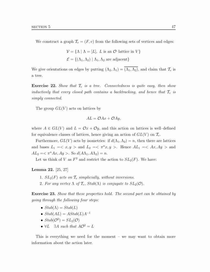
section 5 47
We construct a graph Tv = (F, v) from the following sets of vertices and edges:
V = {Λ | Λ = [L], L is an O–lattice in V }E = {(Λ1,Λ2) | Λ1,Λ2 are adjacent}
We give orientations on edges by putting (Λ2,Λ1) = (Λ1,Λ2), and claim that Tv is
a tree.
Exercise 22. Show that Tv is a tree. Connectedness is quite easy, then show
inductively that every closed path contains a backtracking, and hence that Tv is
simply connected.
The group GL(V ) acts on lattices by
AL = OAx+ OAy,
where A ∈ GL(V ) and L = Ox + Oy, and this action on lattices is well–defined
for equivalence classes of lattices, hence giving an action of GL(V ) on Tv.
Furthermore, GL(V ) acts by isometries: if d(Λ1,Λ2) = n, then there are lattices
and bases L1 =< x, y > and L2 =< πnx, y >. Hence AL1 =< Ax,Ay > and
AL2 =< πnAx,Ay >. So d(AΛ1, AΛ2) = n.
Let us think of V as F 2 and restrict the action to SL2(F ). We have:
Lemma 22. [25, 27]
1. SL2(F ) acts on Tv simplicially, without inversions.
2. For any vertex Λ of Tv, Stab(Λ) is conjugate to SL2(O).
Exercise 23. Show that these properties hold. The second part can be obtained by
going through the following four steps:
• Stab(Λ) = Stab(L)
• Stab(AL) = AStab(L)A−1
• Stab(O2) = SL2(O)
• ∀L ∃A such that AO2 = L
This is everything we need for the moment – we may want to obtain more
information about the action later.

48 section 5
5.2. Some algebraic geometry. Two varieties V,W are birationally equivalent
if there are rational maps ϕ : V → W and ψ : W → V such that ϕ(V ) is dense in
W , ψ(W ) is dense in V , and ϕ ◦ ψ = 1 as well as ψ ◦ ϕ = 1 where defined.
The map J : Cm → CPm defined by J(z1, . . ., zm) = [1, z1, . . ., zm] is a diffeo-
morphism, and if V ⊂ Cm is a variety, then J(V ) is termed a projective completion
of V . In case that V is a 1–dimensional irreducible variety, there is a unique non–
singular projective variety V which is birationally equivalent to J(V ). V is called
the smooth projective completion of V , and the ideal points of V are the points of
V corresponding to J(V ) − J(V ) under the birational equivalence. Moreover, the
function fields of V and V are isomorphic.
5.3. Ideal points and valuations. Let C ⊂ X(M) be a curve, i.e. a 1–dimensional
irreducible subvariety, and denote its smooth projective completion by C. We will
refer to the ideal points of C also as ideal points of C. The function fields of C
and C are isomorphic. Denote them by K. Any ideal point ξ of C determines a
(normalised, discrete, rank 1) valuation ordξ of K, by
ordξ(f) =
k if f has a zero of order k at ξ
∞ if f = 0
−k if f has a pole of order k at ξ
Note that ordξ(z) = 0 for all non-zero constant functions z ∈ C. In the language
of algebraic geometry, the valuation ring {f ∈ K | ordξ(f) ≥ 0} of ordξ is the local
ring at ξ.
5.4. The action. Let C ⊂ X(M) be a curve. We want a representation into SL2 of
a field with a discrete valuation. A good candidate is the tautological representation
P : π1(M) → SL2(F ) of Subsection 4.10. Recall that here, F = C(RC) is the
function field of an irreducible subvariety RC ⊂ R(M) with the property that
t(RC) = C, and F is a finitely generated extension of K = C(C). In order to get
Serre’s tree, we need a suitable valuation on F . To this end, we use the following
extension theorem for valuations:
Lemma 23 (1.1 in [1]). Let F be a finitely generated extension of a field K and
let w : K∗ → ZZ be a valuation of K. Then there exist an integer d > 0 and a
valuation v : F ∗ → ZZ such that v|K∗ = dw.

section 5 49
Note that Ow ⊂ Ov and O∗w ⊂ O∗
v. In particular, the uniformizer in Ow is a d-th
power of a uniformiser in Ov.
The condition of the theorem is satisfied since:
C4n ⊃ C[zi]/J = K ⊃ F = C[yi]/J ⊂ Cm where m = n+
(
n
2
)
+
(
n
3
)
,
where the yi are contained in span{zi}, and we can think of them as trace functions
of generators and ordered double and triple products of generators.
So if we apply the lemma to F , K and the valuation ordx on K, we obtain a
valuation vx on F . We fix our ideal point and write vx = v.
With the valuation v, we can associate a tree Tv on which SL2(F ) acts in the
way described earlier. The tautological representation P : π1(M) → SL2(F ) can
be used to pull the action of SL2(F ) back to an action of π1(M) on Tv, and we
write P(γ) · Λ = γΛ.
This action is simplicial and without inversions by the way SL2(F ) acts. Is it
non–trivial?
5.5. Properties of the action. For each γ ∈ π1(M) we have the function Iγ :
RC → C, defined by Iγ = trP(γ) ∈ K ⊂ F . Since Iγ ∈ K, we may think of it as a
function on C. At an ideal point ξ, it has a well–defined value Iγ(ξ) ∈ C ∪ {∞}.
Lemma 24. [14] For any γ ∈ π1(M) the following are equivalent:
1. Iγ(ξ) ∈ C, i.e. Iγ does not have a pole at ξ.
2. Some vertex of Tv is fixed by γ, where v|K∗ = d · ordξ.
Proof. Note that Iγ(x) ∈ C ⇔ v(Iγ) ≥ 0 ⇔ w(Iγ) ≥ 0 ⇔ Iγ = trP(γ) ∈ O.
(2 ⇒ 1) If a vertex is fixed, then P(γ) is in the stabilizer of the vertex, hence
conjugate to an element in SL2(O). This gives trP(γ) ∈ O.
(1 ⇒ 2) Suppose trP(γ) ∈ O. If P(γ) = ±E, then γ acts trivially on the
tree. Hence assume that P(γ) 6= ±E. Since P(γ) is in the special linear group,
there exists a vector e ∈ K2 such that e and P(γ)e =: f are linearly independent.
With respect to the basis {e, f}, P(γ) has the form
(
0 c
1 d
)
= A−1P(γ)A for
some A ∈ GL2(F ). Now 1 = detP(γ) = −c and d = trP(γ) ∈ O. Thus
P(γ) ∈ ASL2(O)A−1 and fixes a vertex. �
The previous lemma can be generalised as follows:

50 section 5
Lemma 25. A finitely generated subgroup Γ1 of π1(M) fixes a vertex if and only
if Iγ takes a finite value at x for all γ ∈ Γ1.
Proof. The ”only if” follows directly from the first property in Lemma 24, the ”if”
follows from the first property along with Lemma 2. �
Recall that the action of π1(M) on a tree is called non–trivial if π1(M) is not
contained in the stabiliser of a vertex.
Proposition 26. [14] The action of π1(M) on Tv is non–trivial.
Proof. Assume that the action is trivial, then Iγ(x) ∈ C for all γ ∈ π1(M). But
each of our coordinate functions is in particular of the form Iγ for some γ ∈ π1(M)
and at least one of them has to have a pole at an ideal point. This creates a
contradiction. �
Thus, associated to each ideal point of the character variety, there is a non–trivial
action without inversions on a tree, and hence an essential surface. So whenever
there is a curve in X(M) we find an essential surface in M . We have now covered
most of the basic background one needs in order to look at applications.

section 6 51
6. The Weak Neuwirth Conjecture
Let M be a manifold with boundary a single torus. We call the unoriented
isotopy class of a non–trivial simple closed curve in ∂M its slope.
Weak Neuwith Conjecture. Let M be a compact, orientable, irreducible 3–
manifold whose boundary is a single torus. Then either
1. M is a solid torus, or
2. M contains an essential separating annulus, or
3. M contains and essential non–separating torus, or
4. M has at least two boundary slopes.
Proof. ([27], Section 6) We shall deal with the fourth statement in the equivalent
form: If s is any slope, there is an essential surface which has non–empty boundary
and has a boundary slope different from s.
6.1. The case when M is hyperbolic. The proof is easiest if the interior of M
has a finite volume hyperbolic structure. Let s be represented by a curve γ on
∂M and denote the corresponding element in the fundamental group of M by γ.
Consider a component X0 containing a discrete and faithful character. We know
X0 is a curve on which the function Iγ is non–constant. So it must have a pole at
an ideal point x of X0. So we get a tree and an action and a surface S. We need
to show that the surface has non–empty boundary with slope different from s.
So assume that S is closed or that its boundary slope is s. Then γ is isotopic
to a simple closed curve in M − S, and hence γ ∈ im(π1(Mi) → π1(M)) for some
component Mi of M − S. But this implies that γ fixes a vertex and hence Iγ does
not have a pole at x, contradicting our choice of x.
6.2. The other cases. In order to deal with the other cases, we need Thurston’s
Hyperbolisation Theorem:
Thurston’s Hyperbolisation Theorem. If M is a compact, connected, ori-
entable irreducible 3–manifold whose boundary consists of one or more tori, then
its interior admits a hyperbolic structure of finite volume unless M either contains
an essential torus or it is a Seifert fibered space.
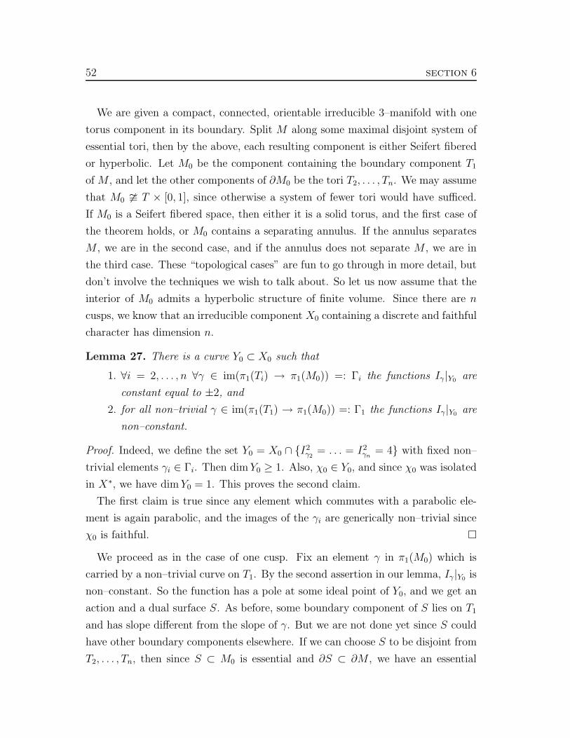
52 section 6
We are given a compact, connected, orientable irreducible 3–manifold with one
torus component in its boundary. Split M along some maximal disjoint system of
essential tori, then by the above, each resulting component is either Seifert fibered
or hyperbolic. Let M0 be the component containing the boundary component T1
of M , and let the other components of ∂M0 be the tori T2, . . . , Tn. We may assume
that M0 � T × [0, 1], since otherwise a system of fewer tori would have sufficed.
If M0 is a Seifert fibered space, then either it is a solid torus, and the first case of
the theorem holds, or M0 contains a separating annulus. If the annulus separates
M , we are in the second case, and if the annulus does not separate M , we are in
the third case. These “topological cases” are fun to go through in more detail, but
don’t involve the techniques we wish to talk about. So let us now assume that the
interior of M0 admits a hyperbolic structure of finite volume. Since there are n
cusps, we know that an irreducible component X0 containing a discrete and faithful
character has dimension n.
Lemma 27. There is a curve Y0 ⊂ X0 such that
1. ∀i = 2, . . . , n ∀γ ∈ im(π1(Ti) → π1(M0)) =: Γi the functions Iγ |Y0are
constant equal to ±2, and
2. for all non–trivial γ ∈ im(π1(T1) → π1(M0)) =: Γ1 the functions Iγ|Y0are
non–constant.
Proof. Indeed, we define the set Y0 = X0 ∩ {I2γ2
= . . . = I2γn
= 4} with fixed non–
trivial elements γi ∈ Γi. Then dimY0 ≥ 1. Also, χ0 ∈ Y0, and since χ0 was isolated
in X∗, we have dimY0 = 1. This proves the second claim.
The first claim is true since any element which commutes with a parabolic ele-
ment is again parabolic, and the images of the γi are generically non–trivial since
χ0 is faithful. �
We proceed as in the case of one cusp. Fix an element γ in π1(M0) which is
carried by a non–trivial curve on T1. By the second assertion in our lemma, Iγ|Y0is
non–constant. So the function has a pole at some ideal point of Y0, and we get an
action and a dual surface S. As before, some boundary component of S lies on T1
and has slope different from the slope of γ. But we are not done yet since S could
have other boundary components elsewhere. If we can choose S to be disjoint from
T2, . . . , Tn, then since S ⊂ M0 is essential and ∂S ⊂ ∂M , we have an essential
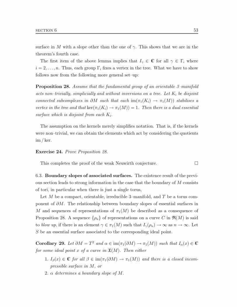
section 6 53
surface in M with a slope other than the one of γ. This shows that we are in the
theorem’s fourth case.
The first item of the above lemma implies that Iγ ∈ C for all γ ∈ Γi where
i = 2, . . . , n. Thus, each group Γi fixes a vertex in the tree. What we have to show
follows now from the following more general set–up:
Proposition 28. Assume that the fundamental group of an orientable 3–manifold
acts non–trivially, simplicially and without inversions on a tree. Let Ki be disjoint
connected subcomplexes in ∂M such that each im(π1(Ki) → π1(M)) stabilises a
vertex in the tree and that ker(π1(Ki) → π1(M)) = 1. Then there is a dual essential
surface which is disjoint from each Ki.
The assumption on the kernels merely simplifies notation. That is, if the kernels
were non–trivial, we can obtain the elements which act by considering the quotients
im / ker.
Exercise 24. Prove Proposition 28.
This completes the proof of the weak Neuwirth conjecture. �
6.3. Boundary slopes of associated surfaces. The existence result of the previ-
ous section leads to strong information in the case that the boundary of M consists
of tori, in particular when there is just a single torus,
Let M be a compact, orientable, irreducible 3–manifold, and T be a torus com-
ponent of ∂M . The relationship between boundary slopes of essential surfaces in
M and sequences of representations of π1(M) be described as a consequence of
Proposition 28. A sequence {ρn} of representations on a curve C in R(M) is said
to blow up, if there is an element γ ∈ π1(M) such that Iγ(ρn) → ∞ as n→ ∞. Let
S be an essential surface associated to the corresponding ideal point.
Corollary 29. Let ∂M = T 2 and α ∈ im(π1(∂M) → π1(M)) such that Iα(x) ∈ C
for some ideal point x of a curve in X(M). Then either
1. Iβ(x) ∈ C for all β ∈ im(π1(∂M) → π1(M)) and there is a closed incom-
pressible surface in M , or
2. α determines a boundary slope of M .
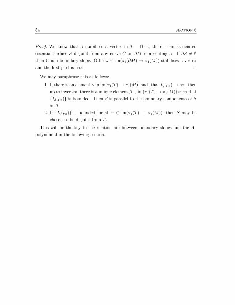
54 section 6
Proof. We know that α stabilises a vertex in T . Thus, there is an associated
essential surface S disjoint from any curve C on ∂M representing α. If ∂S 6= ∅then C is a boundary slope. Otherwise im(π1(∂M) → π1(M)) stabilises a vertex
and the first part is true. �
We may paraphrase this as follows:
1. If there is an element γ in im(π1(T ) → π1(M)) such that Iγ(ρn) → ∞ , then
up to inversion there is a unique element β ∈ im(π1(T ) → π1(M)) such that
{Iβ(ρn)} is bounded. Then β is parallel to the boundary components of S
on T .
2. If {Iγ(ρn)} is bounded for all γ ∈ im(π1(T ) → π1(M)), then S may be
chosen to be disjoint from T .
This will be the key to the relationship between boundary slopes and the A–
polynomial in the following section.
section 7 55
7. Boundary slopes and the A–polynomial
Throughout this section, let M be a 3–manifold with boundary consisting of a
single torus, and fix a generating set {M,L} for the fundamental group of ∂M .
The elements M and L will be referred to as meridian and longitude respectively.
7.1. A–polynomial. The A–polynomial was introduced in [7], and we define it
following [9]. Let RU (M) be the subvariety of R(M) defined by two equations
which specify that the lower left entries in ρ(M) and ρ(L) are equal to zero.
Any representation in R(M) is conjugate to a representation in RU(M) since two
commuting matrices in SL2(C) have a common invariant subspace. We define an
eigenvalue map from RU (M) to (C−{0})2 by taking an element ρ of RU (M) to the
upper left entries of ρ(M) and ρ(L). Taking the closure of the image of this map
and discarding zero–dimensional components, one obtains the eigenvalue variety,
which is necessarily defined by a principal ideal. A generator for the radical of
this ideal is called the A–polynomial. After fixing a basis for the boundary torus,
the A-polynomial is well defined up to multiplication by units in C[l±1, m±1], and
it follows from [7] and [11] that the constant multiple can be chosen such that
the coefficients are all integers with greatest common divisor equal to one. For a
generalisation of the A–polynomial to multi–cusped 3–manifolds, see [33].
Exercise 25. If E is an irreducible component of the eigenvalue variety, show
that (l,m) ∈ E if and only if (l−1, m−1) ∈ E. Hence for each factor AE of the
A—polynomial, we have AE(l,m) = 0 if and only if AE(l−1, m−1) = 0.
The curve defined by the A–polynomial is a useful parameterisation of Dehn
surgery coefficients due to Theorem 19. Note that there is a map from the eigen-
value variety to X(∂M) which generically has degree two. This can be interpreted
as a distinction between the manifolds M(p, q) and M(−p,−q), which is geomet-
rically sensible. Depending on the desired applications and filling curves, one may
want to change from a fixed basis (or framing) for the boundary torus to another.
Exercise 26. How does a change of framing for the boundary torus affect the A—
polynomial? Write down explicit formulae for (M,L) → (M′,L′) and A(l,m) →A(l′, m′).
56 section 7
One generally needs a computer to calculate the A–polynomial, and some com-
putational techniques will be mentioned shortly. It is shown in [7] that if k is a
non–trivial (p, q)–torus knot, then Ak(l,m) is divisible by lmpq +1 (where we follow
the convention that if M is the complement of a knot k in S3, then {M,L} is a
standard peripheral system).
Proposition 30. [33] Let k be a non–trivial (p, q)–torus knot. If p = 2 or q = 2,
then Ak(l,m) = (l− 1)(lmpq + 1), otherwise Ak(l,m) = (l− 1)(lmpq + 1)(lmpq − 1).
Proof. The fundamental group of S3 − k is presented by Γ = 〈u, v | up = vq〉, and
a standard peripheral system is given by M = unvm and L = upM−pq, where
mp + nq = 1. These facts can be found in [6] on page 45. The factor l − 1 arises
from reducible representations, and all factors arising from components containing
irreducible representations are to be determined.
The element up is in the centre of Γ, since it is identical to vq and hence com-
mutes with both generators. Thus the image of up is in the centre of ρ(Γ). Since
two commuting elements have a common eigenvector, ρ(u)p has a common eigen-
vector with ρ(u) and ρ(v) respectively. If the representation is irreducible, these
eigenvectors have to be distinct. Thus, after conjugation it may be assumed that
the generators map to upper and lower triangular matrices respectively, and the
central element is represented by a diagonal matrix. Direct matrix computations
show that the commutativity with either of the generators gives ρ(u)p = ±E.
Assume that ρ(u)p = −E. The relation ρ(L) = −ρ(M)−pq, which is equivalent to
ρ(LMpq) = −E, then implies the equation lmpq = −1. This is the curve obtained
in [7] by sending u and v to non-commuting elements of SL2(C) of order exactly
2p and 2q respectively.
If the image of ρ(u)p is trivial, then ρ(v)q = ρ(u)p = E. If p or q equals 2, this
implies that the image of one of the generators is ±E. But this yields that ρ(Γ)
is abelian, and therefore contradicts the irreducibility assumption. This completes
the proof of the first assertion.
Now assume that neither of p and q is equal to two. As above, curves of irre-
ducible representations are obtained by sending u and v to non-commuting elements
of SL2(C) of order exactly p and q respectively. Any of these curves yields a com-
ponent of the eigenvalue variety defined by the equation lmpq = 1, and this finishes

section 7 57
the proof of the proposition. In fact, with a more precise analysis one could count
the number of 1–dimensional curves in the character variety of a torus knot. �
Exercise 27. How many curves are in the character variety of the (p, q)–torus
knot?
7.2. A–polynomial. Analogous to the SL2(C)–eigenvalue variety, there is an
eigenvalue variety associated to the PSL2(C)–character variety. This is the variety
containing points corresponding to pairs of squares of eigenvalues of the meridian
and longitude (in the case where the boundary of M consists of a single torus).
A generator for its defining (principal) ideal is the A–polynomial, and its vari-
ables have the unfortunate names L and M . Thus, AM(L,M) is the A–polynomial
associated to the manifold M .
Proposition 31. [33] Let k be a non–trivial (p, q)–torus knot. Then Ak(L,M) =
(L− 1)(LMpq − 1).
Proof. It follows from Exercise 17 that all PSL2(C)–representations of a knot group
lift to SL2(C). Thus, all factors of the A–polynomial arise from factors of the A–
polynomial and vice versa.
The eigenvalue of the meridian appears with even powers in the (unfactorised)
A–polynomial of k, and the sign of the longitude’s eigenvalue is uniquely determined
since L is null–homologous. Thus, Ak(l,m) = Ak(l,−m), but Ak(l,m) = 0 does
not imply Ak(−l,m) = 0 in general. However, since Ak(l2, m2) = Ak((−l)2, m2), it
follows that the variety defined by Ak(l2, m2) = 0 is the locus ofAk(l,m)Ak(−l,m) =
0. Expanding Ak(l,m)Ak(−l,m) = 0, substituting l2 = L andm2 = M and deleting
repeated factors therefore gives the result as stated. �
7.3. Elimination theory. Calculations of the A–polynomial (and also of char-
acter varieties) often use the elimination and extension theorems as found in
[12]. Given two polynomials f1, f2 ∈ C[x1, . . ., xm] of positive degree in x1, let
g1, g2 ∈ C[x2, . . ., xm] such that fi = gixni
1 + terms in which x1 has degree lower
than ni. The resultant Res(f1, f2, x1) (whose definition we omit) is an element of
C[x2, . . ., xm]. If this resultant vanishes at P = (p2, . . ., pm) and not both of g1 and
g2 vanish at P , then there is p1 ∈ C such that f1 and f2 vanish at (p1, . . ., pm).
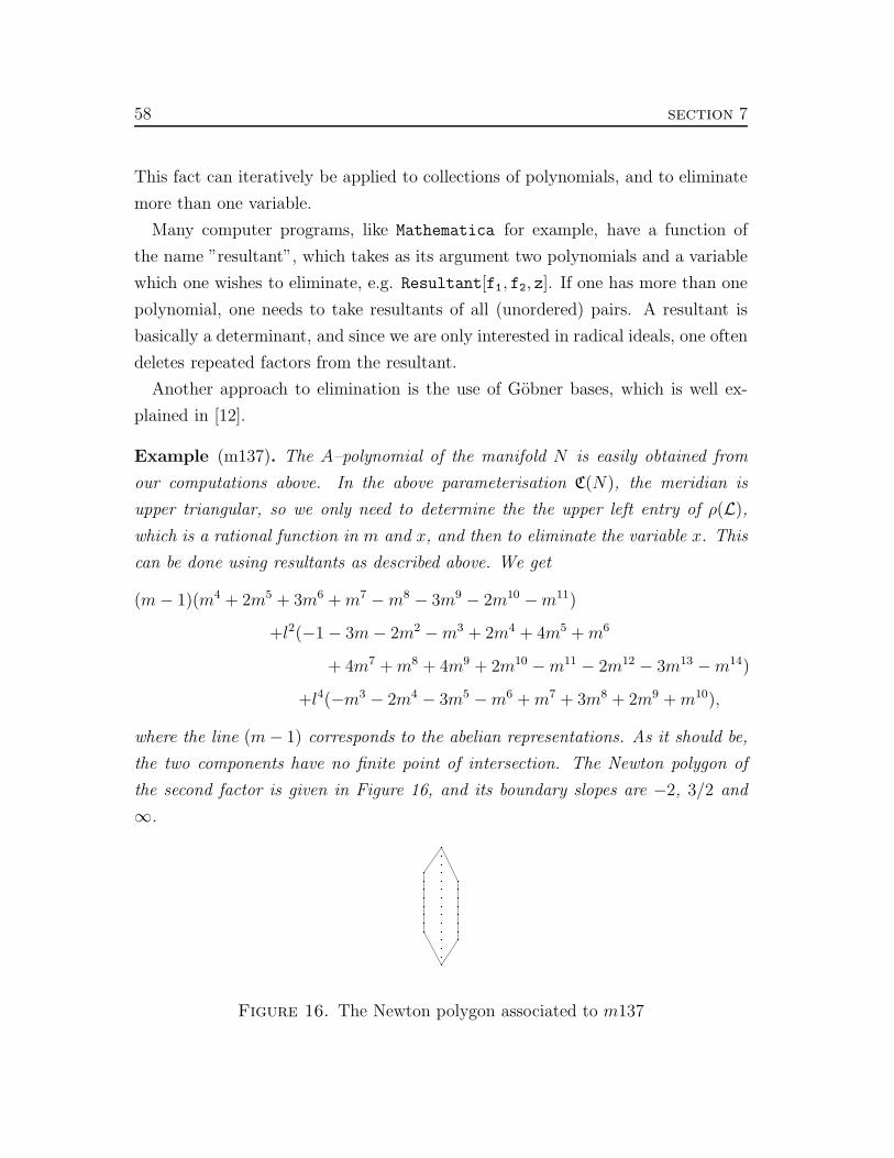
58 section 7
This fact can iteratively be applied to collections of polynomials, and to eliminate
more than one variable.
Many computer programs, like Mathematica for example, have a function of
the name ”resultant”, which takes as its argument two polynomials and a variable
which one wishes to eliminate, e.g. Resultant[f1, f2, z]. If one has more than one
polynomial, one needs to take resultants of all (unordered) pairs. A resultant is
basically a determinant, and since we are only interested in radical ideals, one often
deletes repeated factors from the resultant.
Another approach to elimination is the use of Gobner bases, which is well ex-
plained in [12].
Example (m137). The A–polynomial of the manifold N is easily obtained from
our computations above. In the above parameterisation C(N), the meridian is
upper triangular, so we only need to determine the the upper left entry of ρ(L),
which is a rational function in m and x, and then to eliminate the variable x. This
can be done using resultants as described above. We get
(m− 1)(m4 + 2m5 + 3m6 +m7 −m8 − 3m9 − 2m10 −m11)
+l2(−1 − 3m− 2m2 −m3 + 2m4 + 4m5 +m6
+ 4m7 +m8 + 4m9 + 2m10 −m11 − 2m12 − 3m13 −m14)
+l4(−m3 − 2m4 − 3m5 −m6 +m7 + 3m8 + 2m9 +m10),
where the line (m− 1) corresponds to the abelian representations. As it should be,
the two components have no finite point of intersection. The Newton polygon of
the second factor is given in Figure 16, and its boundary slopes are −2, 3/2 and
∞.
Figure 16. The Newton polygon associated to m137
section 7 59
We will need the following facts in order to prove the main result of this section.
7.4. Newton polytopes. Let f ∈ C[X±11 , ..., X±1
m ] be given as an expression f =∑
α∈ZZm aαXα. Then the Newton polytope of f is the convex hull of s(f) = {α ∈
ZZm | aα 6= 0}. Thus, if s(f) = {α1, . . ., αk}, then
(7.1) Newt(f) = Conv(s(f)) =
{ k∑
i=1
λiαi | λ ≥ 0,k∑
i=1
λi = 1
}
.
Note that Newt(0) = ∅, and since V (0) = (C − {0})m, we have V (0)∞ = Sm−1.
For arbitrary subsets A,B of IRm, let A +B = {a+ b | a ∈ A, b ∈ B}.
Exercise 28. [12]
1. Let f, g ∈ C[X±] such that fg 6= 0. Then Newt(fg) = Newt(f)+Newt(g).
2. Newt(f + g) ⊆ Conv(s(f) ∪ s(g)) = Conv(Newt(f) ∪Newt(g)).
7.5. Spherical duals. The set of outward pointing normal vectors can be de-
scribed using spherical duals. The spherical dual of a bounded convex polytope P
in IRm is the set of vectors ξ of length 1 such that the supremum supα∈P α · ξ is
achieved for more than one α, and it is denoted by Sph(P ). Geometrically, Sph(f)
consists of all outward unit normal vectors to the support planes of P which meet
P in more than one point. If P is the Newton polytope of a non–zero polynomial
f , then the spherical dual of Newt(f) is also denoted by Sph(f).
Spherical duals are easy to visualise in low dimensions. Given a convex polygon
P in IR2, its spherical dual is the collection of points on the unit circle defined by
outward pointing unit normal vectors to edges of P . Given a convex polyhedron in
IR3, we obtain the vertices of its spherical dual again as points on the unit sphere
S2 arising from outward pointing unit normal vectors to faces. We then join two
of these points along the shorter geodesic arc in S2 if the corresponding faces have
a common edge. This gives a finite graph in S2.
Exercise 29. [33] Let f, g ∈ C[X±]. If fg 6= 0, then Sph(fg) = Sph(f)∪ Sph(g).
7.6. Slopes are slopes. We are now in a position to prove the ”boundary slopes”
theorem which was stated in the introduction.
60 section 7
Theorem 32. [7] Let M be a compact, orientable, irreducible 3–manifold with
boundary consisting of a single torus. The slopes of edges of the Newton Poly-
gon of the A–polynomial are the boundary slopes of essential surfaces in the knot
complement.
Proof. Since the boundary of M is a torus, we choose a basis {M,L} for this torus.
Assume that C ⊂ X(M) is a curve with the property that the associated component
E in the eigenvalue variety is a curve. Let the factor of the A–polynomial defining
E be AE(l,m) =∑
(i,j)∈A c(i, j)milj where A ⊂ ZZ2 is a finite set and c(i, j) 6= 0.
We have a component RC of RU (M) such that t(RC) = C, and a tautological
representation P : π1(M) → SL2(F ) where F is a finitely generated extension of
C(C). We may assume that P is upper triangular on the meridian M. Then F is
also a finitely generated extension of C(E), since we obtain a regular map RC → E
by restriction to the upper left entries m of P(M) and l of P(L).
Let x be an ideal point of E. We consider the discrete valuation ordx of C(E).
By the extension lemma, this extends to a valuation of F . Since x is an ideal point,
at least one of the coordinate functions m or l approaches 0 or ∞, and hence at
least one of the functions m + m−1 or l + l−1 blows up. (Note that the argument
given here also works if we regard E as a variety in C2 since eigenvalues on E come
in pairs (m, l) and (m−1, l−1).)
Assume that ordx(m) = −a and ordx(l) = −b, where a, b ∈ ZZ are co-prime
and at least one of them is not zero since x is an ideal point and the valuation
is normalised, discrete, rank 1. Then the eigenvalue of the element M−bLa has
valuation ordx(m−bla) = ab − ba = 0. This implies that IM−bLa stays finite at x,
and the results of Subsection 6.3 imply that M−bLa hence determines a boundary
slope of M , which we also write as −b/a.To know all detected boundary slopes, we therefore need to determine (up to
scaling) the possible valuations v which arise at ideal points of components of the
eigenvalue variety. Assume that v is such a valuation with v(m) = −a, v(l) = −b.
For simplicity, write ξ =
(
a
b
)
. We can compute the valuation of a monomial using
the Euclidean dot product: v(milj) = −ξ ·(
i
j
)
.

section 7 61
Now AE(l,m) =∑
c(i, j)milj vanishes on the curve defined by it if and only if
v(AE) = v(0) = ∞. This is the case only if the monomials that blow up fastest
cancel, i.e. only if the minimum of the terms v(milj) = −ξ ·(
i
j
)
, (i, j) ∈ A, is
assumed at least twice. Conversely, there is a result due to Bergman [3], which
asserts that if this minimum is attained at least twice, then one can define a
valuation v which satisfies v(AE) = ∞ and v(m) = −a and v(l) = −b.Thus, we have a valuation v with v(AE) = ∞ if and only if the maximum of
the terms v(milj) = ξ ·(
i
j
)
, (i, j) ∈ A, is assumed at least twice. This is the
case if and only if ξ is an outward pointing normal vector to a support plane of
the Newton polygon of AE , hence if and only if −b/a is the slope of a side of the
Newton polygon.
Putting everything together, we see that if −b/a is the slope of a side of the
Newton polygon of AE , then −b/a is the slope of an essential surface in M . The
result now follows from Exercise 29, which implies that the set of boundary slopes
of the Newton polygon of a polynomial is the union of the boundary slopes of the
Newton polygons of its irreducible factors. �
62 section 8
8. Representations and the Alexander polynomial
This section does not contain an application of Culler–Shalen theory, but has a
common theme with the previous and the next section: eigenvalues. Following [7],
we interpret non–abelian reducible representations of knot groups as representa-
tions into the affine group of the complex plane, and obtain a relationship to zeros
of the Alexander polynomial.
8.1. Alexander module. Let M = S3 − ν(k). Then there is a covering p : C∞ →M , such that p∗(π1(C∞)) = Γ′, where Γ′ denotes the commutator subgroup of Γ,
and the group of covering transformations is infinite cyclic. This covering is called
the infinite cyclic covering. The induced homomorphism p∗ is injective, we have
π1(C∞) ∼= Γ′, and the first homology group of C∞, H1(C∞), is isomorphic to Γ′/Γ′′.
Recall that Γ is a semidirect product Γ = ZnΓ′, where Z ∼= Γ/Γ′ is infinite cyclic
by Proposition 11. Choose a meridian t of Γ as a representative of a coset of Z.
Since Z acts by conjugation on the commutator subgroup, and since commutator
subgroups are characteristic, this induces an action on Γ′/Γ′′:
g → t−1gt for g ∈ Γ′/Γ′′.
We denote this action by g → tg. This induced action is independent of the choice
of the representative t in tΓ′, since any other representative which is a pullback
of the generating element under Γ → Z gives an action which differs by an inner
automorphism of Γ. Furthermore, we can regard Γ′/Γ′′ as a finitely presented ZZ(t)-
module, ZZ(t) = ZZ[t, 1/t], which is called the Alexander module M(t) of the knot
group Γ.
In other words, the Alexander module is H1(C∞) and the group of covering
transformations induces the module operation. The elements ζ ∈ ZZ(t) such that
ζ(h) = 0 for all h ∈ H1(C∞) form an ideal I. It can be shown that this ideal
is principal. The defining polynomial of this ideal is denoted by ∆k and called
the Alexander polynomial of k. The Alexander polynomial is therefore a general
relation in H1(C∞), and it is defined up to units, i.e. up to ±tn.
Take a (m × n) presentation matrix A(t) of the Alexander module, which we
shall refer to as an Alexander matrix. We can calculate the Alexander polynomial
section 8 63
algebraically as the greatest common divisor of the elements of the ideal generated
by the (n× n) minors of A(t). This is invariant under Tietze transformations.
Consider the epimorphism ϕ : Γ → ZZ given by ϕ(g) = lk(g, k). Choose a
presentation of Γ =< g0, . . . , gn | r1, . . . , rn >, which has one generator more than
relations, and perform basis transformations such that we have a presentation where
ϕ(g0) = 1 and ϕ(gi) = 0 for all i ∈ {1, . . . , n}. Then gi ∈ Γ′ for i ∈ {1, . . . , n},and Γ′ =< gi | r1, . . . , rn > is a presentation of Γ′ as an ZZ(t)–module. Passing to
H1(C∞), we have to abelianise Γ′, and the Alexander polynomial follows from the
relations.
8.2. Metabelian representations. Any abelian homomorphic image of a knot
group is cyclic. Apart from abelian representations there are other reducible rep-
resentations which have to be metabelian by the condition on the trace of elements
in the commutator group in Lemma 13:
Exercise 30. Show that a non-abelian reducible representation of a finitely gen-
erated group Γ into SL2(C) is metabelian, i.e. that the image of Γ′′ = [Γ′,Γ′] is
trivial.
Assume that ρ : Γ → H is a surjective homomorphism, where H is a metabelian
group (not necessarily a subgroup of SL2(C)). Since Γ = Z n Γ′, we have
H = ρ(Γ) = ρ(Z) n ρ(Γ′) = ρ(Z) nH ′,
since the commutator subgroup is characteristic. Assume that ρ(Z) is infinite cyclic.
Then H ′ can be considered as a ZZ(t)–module. Since H is metabelian, H ′ is abelian,
and we have the following unique factorisation:
Z n Γ′ ϕ−−−→ Z nH ′
y
x
Z n Γ′/Γ′′ Z nH1(C∞)
Thus, we factor through the first homology group of the infinite cyclic covering,
which is the Alexander module, and the operation is defined by the operation of
the semidirect product. This shows that any metabelian representation of a knot
group Γ factors through G → Z nH1(C∞).

64 section 8
Let Γ =< g0, . . . , gn | r0, . . . , rn > be a Wirtinger presentation. We have already
observed that lk(gi, k) = 1 for all i ∈ {0, . . . , n}. We now change the basis to the
set {g0, h1, . . . , hn} where hi = gig−10 for i ∈ {1, . . . , n}. Thus lk(hi, k) = 0 and
hence hi ∈ Γ′.
The relations are of one of the following forms:
rj = gjg−1i g−1
k gi,(W1)
rj = gjgig−1k g−1
i .(W2)
Using the equivalent presentation, we get
rj = hjh−1i g−1
0 h−1k hig0(W1’)
= hjh−1i (g−1
0 h−1k g0)(g
−10 hig0),
rj = hjg0hih−1k g−1
0 h−1i(W2’)
= hj(g0hig−10 )(g0h
−1k g−1
0 )h−1i .
As described above, we get any metabelian representation via factorisation through
H1(C∞). Writing H1(C∞) additively, conjugation by g0 becomes multiplication by
t, and we have the relations:
rj = hj − hi − thk + thi,(A1)
rj = hj +1
thi −
1
thk − hi.(A2)
The matrix corresponding to this system of equations is the Alexander matrix,
and its determinant is the Alexander polynomial. In order to find metabelian
representations into SL2(C), we will now take a small detour.
8.3. Affine representations. Consider a metabelian representation ρ of the knot
group Γ into the affine group Af(C) of the complex plane. Let ρ(Γ) = H and
assume that H ′ is nontrivial. We may conjugate this representation such that the
fixed point of ρ(g0) is zero, if we assume that the derivative of ρ(g0) is not equal to
one. Otherwise the representation would be abelian, which contradicts our choice.
Thus, ρ(g0) = f0(z) = tz for some complex number t. Since all meridians are
conjugate, we have ρ(gi) = fi(z) = tz + hi for all i ∈ {1, . . . , n}, i.e. the images of
meridians have the same derivative.
section 8 65
Setting the image of an relator equal to the identity, gives homogeneous linear
equations in h1, . . . , hn. It can easily be verified that this system of equations is
identical to the system of equations given by (A1) and (A2). Starting with the
relations (W1) and (W2), we get:
z = z + hj − hi − thk + thi,(A1’)
z = z + hj +1
thi −
1
thk − hi.(A2’)
Clearly, ρ gives a nonabelian representation if and only if some of the hi are
nonzero. This is the case if and only if the system of equations has a nonzero
solution. Note that if all hi = 0, then H ′ is trivial, and H abelian.
Therefore, there exists a nonabelian affine representation of Γ for which the
image of each meridian has derivative t if and only if t is a zero of the Alexander
polynomial.
Since we are interested in representations into SL2(C), consider the composite
mapping:
fi(z) = tz + hiι−→(
t hi
0 1
)
µ−→(√
t−1
0
0√t−1
)(
t hi
0 1
)
=
(√t hi
√t−1
0√t−1
)
.
Here, we have first mapped affine transformations into GL2(C). Left multiplica-
tion is a bijective mapping of a group, which in this case yields elements in SL2(C).
We claim that this composite mapping gives us a representation of Γ into SL2(C).
For this, we perform the following matrix computation:(√
t hi
√t
0√t−1
)(√t hj
√t
0√t−1
)
=
(
t hj + t−1hi
0 t−1
)
Thus, the composite mapping respects the composition of affine transformations,
and only the identity f(z) = z is contained in its kernel, so µι is a monomorphism.
This yields a representation of Γ into SL2(C). The commutator of two elements is
upper triangular with entries equal to one on the diagonal. Thus, the representation
is reducible by Lemma 13.
This shows that there is a reducible representation of Γ into SL2(C), which has
non-abelian image and sends a meridian to an element with eigenvalue ±√t, if t is
a root of ∆k.
66 section 8
8.4. Conclusion. We now wish to prove the following:
Proposition 33. [7] The following are equivalent:
1. There exists a reducible representation of Γ(k) into SL2(C) which has non-
abelian image and sends a meridian to an element with eigenvalue m.
2. m2 is a root of ∆k.
Proof. One direction has already been shown. Now assume that there exists a
reducible representation of Γ in SL2(C) which has non-abelian image and sends a
meridian to an element with eigenvalue m. We may assume that the meridians are
upper triangular matrices, and that the upper left entry of some meridian is m.
Consider the following mapping:(
m h
0 m−1
)
→ m2z + hm.
This gives a homomorphism from the subgroup of all upper triangular matrices
in SL2(C) to the group of affine motions of the complex plane. Since the group
was supposed to be metabelian, this is the case if and only if m2 is a zero of the
Alexander polynomial. �
We conclude that the eigenvalues m of meridians in metabelian representations
are invariants of the knot — however, this information is already contained in the
Alexander polynomial.
Proposition 34. [7] Suppose that ρ is a reducible representation of a knot group
Γ(k) such that the character of ρ lies on a component of X(Γ) which contains the
character of an irreducible representation. If γ is a meridian of Γ, then ρ(γ) has
eigenvalue m where m2 is a root of the Alexander polynomial of k.
Proof. It is sufficient to show that there is a reducible non-abelian representation
with the same character as ρ. We have dim t−1(y) ≥ 3 for all points y of a com-
ponent which contains the character of an irreducible representation. It is stated
in Exercise 15 that the variety of abelian representations with a given character is
2–dimensional. Since the dimensions of points in the same component are to be
equal, t−1(t ρ) contains a representation with nonabelian image. �
section 9 67
9. The Roots of Unity Phenomenon
Let us assume that a surface S is associated to an ideal point of the character
variety of a manifold M . We know that the “character” at the ideal point takes
finite values when restricted to components of M − S, and hence corresponds
to representations of these pieces. However, since we are at an ideal point of
the character variety, these representations cannot be glued together to form a
representation of the manifold.
In the present section, we will deduce a little more information about the char-
acters at infinity. It turns out that they are reducible on the associated surface.
This observation leads to the roots of unity phenomenon, but also gives a necessary
condition on a surface to be detected.
Reference. [7], Section 5.
9.1. Reduced Surfaces. Let M be a compact, orientable, irreducible 3–manifold
with boundary consisting of a single torus. Assume that there is an ideal point ξ of
a curve C in X(M) with the property that Iγ(ξ) = ∞ for some γ ∈ im(π1(∂M) →π1(M)). This ensures that an essential surface S which is associated to the action
of π1(M) on Tv determined by P has non–empty boundary. The boundary compo-
nents of S are a family of parallel simple closed curves on the torus ∂M , so they all
lie in the same homotopy class. Let h be a representative of the particular homo-
topy class, and let I∂S(ξ) = Ih(ξ). This is well–defined since the trace is invariant
under conjugation and taking inverses.
A surface is called reduced if it has the minimal number of boundary components
amongst all associated essential surfaces. Let n(S) denote the greatest common
divisor of the number of boundary components of the components of S.
Theorem 35. [7] Let M be a compact, orientable, irreducible 3–manifold with
boundary consisting of a single torus, and let ξ be an ideal point of a curve C in
X(M) with the property that Iγ(ξ) = ∞ for some γ ∈ im(π1(∂M) → π1(M)).
Let S be a surface associated to the action of π1(M) on Tv determined by P.
Then I∂S(ξ) = λ+ λ−1, where λ is a root of unity. Moreover, if S is reduced, then
λn(S) = 1.
68 section 9
In order to prove this theorem, we will have to establish more facts about our
action.
9.2. Edges and eigenvalues. Going back to what we have learnt about actions
on trees: what does an element A ∈ SL2(F ) look like if it fixes an edge (Λ1,Λ2)?
Exercise 31. If A ∈ Stab(Λ1,Λ2), then A is of the form
(
a b
c d
)
where a, b, d ∈ O
and c ∈ πO. Furthermore, any element in the commutator group of Stab(Λ1,Λ2)
has trace equal to 2 mod (π). You can show this directly or using the induced
action of A on the residue field k = O/(π).
Now let A ∈ SL2(F ) be any element in the stabilizer of our edge. We know that
we can find representatives L1 and L2 such that the proper inclusions
πL1 & L2 & L1
hold. Passing to the quotient space L1/πL1, which is a 2–dimensional k-vector
space, the above inclusions give
0 & L2/πL1 & L1/πL1.
So L2/πL1 is a non–trivial proper subspace, hence a 1–dimensional subspace. The
matrix A induces a linear transformation on the quotient space, which stabilises
L2/πL1. Thus, it multiplies this line by an element λ ∈ k = O/(π), which we call
an eigenvalue associated to our fixed edge.
Exercise 32. The eigenvalue associated to an edge is independent upon the choice
of lattice representatives.
Note that the eigenvalue was only dependent upon the choice of orientation of
the edge. We claim that
Lemma 36. The eigenvalue of A associated to (Λ1,Λ2) = (Λ2,Λ1) is λ−1.
Proof. The above inclusions imply that
πL2 & πL1 & L2.

section 9 69
So if λ is the eigenvalue associated to (Λ2,Λ1), then A induces multiplication by
this value on πL1/πL2∼= L1/L2. The latter suggests that we ought to look at the
exact sequence
0 → L2/πL1 → L1/πL1 → L1/L2 → 0.
Thus, we have found the eigenvalues corresponding to two direct summands of
L1/πL1, and hence λλ is the image of detA in k. Since A ∈ SL2(F ), this proves
the claim. �
Since the action is without inversions, A fixes the initial and terminal vertices of
our edge, and hence trA ∈ O. If λ is the eigenvalue associated to the edge, then
λ+ λ−1 is the image of trA under the quotient map.
9.3. Comparable edges. An edge path in T is a sequence e0, . . . , en of edges in
T such that i(ej) = t(ej−1) for j = 1, . . . , n. The edge path is reduced if there is no
backtracking, i.e. ej 6= ej−1 for j = 1, . . . , n.
We can define a partial ordering on T by setting e ≤ f if there is a reduced edge
path with e0 = e and en = f . Thus, for any pair of distinct edges, exactly one of
the following relationships holds:
e < f, e < f, f < e, f < e.
By the preceding section, if A ∈ SL2(F ) fixes two edges, then the associated
eigenvalues are either the same or inverses.
Exercise 33. Assume A fixes the edges (Λ1,Λ) and (Λ2,Λ). If the eigenvalue
associated to the first edge is λ, then the eigenvalue associated to the latter is λ−1.
Moreover, if A fixes the first and last edge of a reduced edge path, then it fixes
each edge in between and the associated eigenvalues are all equal.
9.4. Compatibly oriented curves. Let us go back to our manifold, and fix ori-
entations of M and S. Then ∂M and p−1(∂S) have induced orientations. Fur-
thermore, the components of S and ∂S have induced transverse orientations in M
and ∂M . To save us some time, assume that the boundary of M is incompressible.
Then the components of ∂M are planes and the components of p−1(∂S) contained
in a connected component of ∂M form a family of parallel lines. We say that two
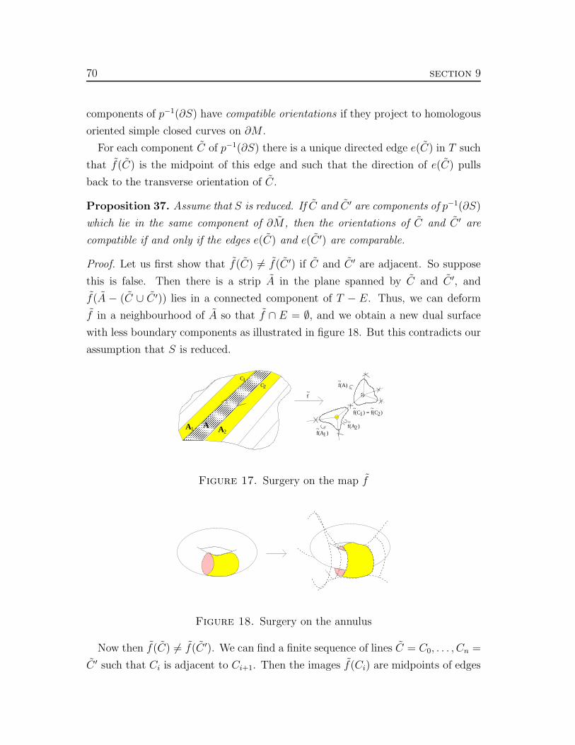
70 section 9
components of p−1(∂S) have compatible orientations if they project to homologous
oriented simple closed curves on ∂M .
For each component C of p−1(∂S) there is a unique directed edge e(C) in T such
that f(C) is the midpoint of this edge and such that the direction of e(C) pulls
back to the transverse orientation of C.
Proposition 37. Assume that S is reduced. If C and C ′ are components of p−1(∂S)
which lie in the same component of ∂M , then the orientations of C and C ′ are
compatible if and only if the edges e(C) and e(C ′) are comparable.
Proof. Let us first show that f(C) 6= f(C ′) if C and C ′ are adjacent. So suppose
this is false. Then there is a strip A in the plane spanned by C and C ′, and
f(A − (C ∪ C ′)) lies in a connected component of T − E. Thus, we can deform
f in a neighbourhood of A so that f ∩ E = ∅, and we obtain a new dual surface
with less boundary components as illustrated in figure 18. But this contradicts our
assumption that S is reduced.
����
� � � � � � � � � � � � � � � � � � � � �� � � � � � � � � � � � � � � � � � � � �� � � � � � � � � � � � � � � � � � � � �� � � � � � � � � � � � � � � � � � � � �� � � � � � � � � � � � � � � � � � � � �� � � � � � � � � � � � � � � � � � � � �� � � � � � � � � � � � � � � � � � � � �� � � � � � � � � � � � � � � � � � � � �� � � � � � � � � � � � � � � � � � � � �� � � � � � � � � � � � � � � � � � � � �� � � � � � � � � � � � � � � � � � � � �� � � � � � � � � � � � � � � � � � � � �� � � � � � � � � � � � � � � � � � � � �� � � � � � � � � � � � � � � � � � � � �� � � � � � � � � � � � � � � � � � � � �� � � � � � � � � � � � � � � � � � � � �� � � � � � � � � � � � � � � � � � � � �� � � � � � � � � � � � � � � � � � � � �� � � � � � � � � � � � � � � � � � � � �� � � � � � � � � � � � � � � � � � � � �� � � � � � � � � � � � � � � � � � � � �� � � � � � � � � � � � � � � � � � � � �� � � � � � � � � � � � � � � � � � � � �� � � � � � � � � � � � � � � � � � � � �� � � � � � � � � � � � � � � � � � � � �� � � � � � � � � � � � � � � � � � � � �� � � � � � � � � � � � � � � � � � � � �� � � � � � � � � � � � � � � � � � � � �� � � � � � � � � � � � � � � � � � � � �� � � � � � � � � � � � � � � � � � � � �� � � � � � � � � � � � � � � � � � � � �� � � � � � � � � � � � � � � � � � � � �� � � � � � � � � � � � � � � � � � � � �
� � � � � � � � � � � � � � � � � � � � �� � � � � � � � � � � � � � � � � � � � �� � � � � � � � � � � � � � � � � � � � �� � � � � � � � � � � � � � � � � � � � �� � � � � � � � � � � � � � � � � � � � �� � � � � � � � � � � � � � � � � � � � �� � � � � � � � � � � � � � � � � � � � �� � � � � � � � � � � � � � � � � � � � �� � � � � � � � � � � � � � � � � � � � �� � � � � � � � � � � � � � � � � � � � �� � � � � � � � � � � � � � � � � � � � �� � � � � � � � � � � � � � � � � � � � �� � � � � � � � � � � � � � � � � � � � �� � � � � � � � � � � � � � � � � � � � �� � � � � � � � � � � � � � � � � � � � �� � � � � � � � � � � � � � � � � � � � �� � � � � � � � � � � � � � � � � � � � �� � � � � � � � � � � � � � � � � � � � �� � � � � � � � � � � � � � � � � � � � �� � � � � � � � � � � � � � � � � � � � �� � � � � � � � � � � � � � � � � � � � �� � � � � � � � � � � � � � � � � � � � �� � � � � � � � � � � � � � � � � � � � �� � � � � � � � � � � � � � � � � � � � �� � � � � � � � � � � � � � � � � � � � �� � � � � � � � � � � � � � � � � � � � �� � � � � � � � � � � � � � � � � � � � �� � � � � � � � � � � � � � � � � � � � �� � � � � � � � � � � � � � � � � � � � �� � � � � � � � � � � � � � � � � � � � �� � � � � � � � � � � � � � � � � � � � �� � � � � � � � � � � � � � � � � � � � �� � � � � � � � � � � � � � � � � � � � �
f(C ) = f(C )1 2~ ~
f(A)~
f(A )f(A )
12~
~
f~
A1 A A2
C1C2
Figure 17. Surgery on the map f
Figure 18. Surgery on the annulus
Now then f(C) 6= f(C ′). We can find a finite sequence of lines C = C0, . . . , Cn =
C ′ such that Ci is adjacent to Ci+1. Then the images f(Ci) are midpoints of edges
section 9 71
in a reduced path e0, . . . , en, where ei is equal to e(Ci) or e(Ci). We know that e0
and en are comparable. If the orientations of C and C ′ are compatible, then either
e0 = e(C) and en = e(C ′) or e0 = e(C) and en = e(C ′). �
9.5. Proof of Theorem 35. Let S0 be a component of S with non–empty bound-
ary, and pick a component S0 of p−1(S0). The group π1(S0) stabilises S0 and
hence an edge e in the tree. We assume that e is directed to match the transverse
orientation of S0.
A component of ∂S0 determines a conjugacy class in π1(S0), and hence a con-
jugacy class in Stab(e). Choose a representative h of this class, and denote the
eigenvalue of h associated to e by λC .
Now list all boundary components of S0, say C1, . . . , Cn. For each component,
let hi be an element of π1(S0) in the conjugacy class determined by Ci with the
induced orientation. Since the image of S0 was the midpoint of the edge e, each hi
is contained in Stab(e) with associated eigenvalue λi = λCi. Since S is a connected
surface, the product h1 · · ·hn is an element of the commutator group of π1(S0) and
hence of the commutator group of the stabilizer of an edge. By the results from one
of the earlier sections, we know that h1 · · ·hn has associated eigenvalue λ1 · · ·λn
and that λ1 · · ·λn = 1 mod π.
We claim that λi = λ±11 for all i. Let Ci be lifts of the boundary components of
S0 to a connected component U of p−1(∂M) with corresponding lifts of S0 for each
i. We have f(Ci) = ei for some edges in T .
Now h1 is a deck transformation of the covering of the torus ∂M by U and leaves
the line C1 invariant. It also preserves the whole family of lines U ∩ p−1(∂S), and
hence in particular each Ci.
So for each i, either h1 or h−11 is the generator of Stab(Ci), depending upon
whether the orientations of C1 and Ci are compatible. This implies that λi = λ±11
for all i. Putting λ1 = λ, this gives λm = 1 in the residue field for some m. Now
tr ∂S = λ+ λ−1 and this proves the first part of the theorem.
Claim. If S is a reduced surface and if C and C ′ are boundary components of S0,
then λC = λC′.
Proof. By the above, we know that either h or h−1 is the generator of Stab(C ′),
depending upon whether the orientations of C and C ′ are compatible. Since S is
72 section 9
reduced, we also know that the edges e and e′ are comparable if and only if the
orientations of C and C ′ are compatible.
Putting all of this together gives that if the orientations of C and C ′ are com-
patible, then h generates both stabilisers, and we have the same eigenvalue. If the
orientations are not compatible, then the edges are not comparable, and λ−1C′ is the
eigenvalue of h associated to e′, and again λC = λC′. �
So if S is reduced, we have that all eigenvalues associated to the components of
∂S0 are equal, which gives the equality λn = 1 in the residue field. Since S0 was
an arbitrary component of the surface S, we have proved Theorem 35.
9.6. Non-trivial roots. Given the main theorem in this section, we see that know-
ing the trace of the unique boundary slope can give us information about associated
reduced surfaces. However, if the trace is just 2 or −2, we don’t get much extra
information. So let us call a root of unity non–trivial if it is not equal to ±1. The
first examples with non–trivial roots of unity associated to a boundary slope were
found by Nathan Dunfield in [15], and the manifold m137 was one of them.
Example. Going back to the tautological representation of m137 on page 39, it is
not hard to work out that the ideal points of the character variety are encoded in
the numerator of the expression given for the coordinate y. If we write the ideal
points naively as tuples (m, x), and let ξk denote a non–trivial k–th root of unity,
we have the following cases and results:
• (1, 0): The longitude has an eigenvalue equal to 0.
• (ξ3, 0): The longitude has an eigenvalue equal to 0.
• (0, ξ6): The element M2L−1 has eigenvalues equal to 1.
• (0, ξ3): The element M2L−1 has eigenvalues equal to −1.
• (0, ξ4): The element M3L2 has eigenvalues equal to −1.
This behaviour can be observed as follows. Firstly, we use the A-polynomial. As
m tends to one of the third roots of unity, the eigenvalue of the longitude tends to
zero, and we are done for the ideal points where x→ 0, since M is now a boundary
slope.
We then perform a basis transformation on the torus such that L → M2L−1.
As m → 0, we obtain the two eigenvalues 1 and −1 for M2L−1 from above. We
section 9 73
use our tautological representation, determine the upper left entry of M2L−1, and
find that as x tends towards one of the third or sixth roots of unity, the limit is well
defined and as stated above. As the approaches x → ±i are well defined, as well,
but give eigenvalues equal to 0 for M2L−1, the slope −2 is not associated to these
ideal points.
So if we have classified the ideal points correctly, the points (0, ξ4) should corre-
spond to the slope 3/2. In order to determine the roots of unity associated to the
slope, we may again perform basis transformations on the torus, which gives the
stated eigenvalue of the element M3L2. We may use this information to verify in
the tautological representation that (0, ξ4) are the corresponding points at infinity.
Thus, we only find non–trivial roots associated to boundary slopes in the second
item above. Applying the main result from this section, we deduce that reduced dual
surfaces associated to the ideal points (ξ3, 0) have 3k boundary components for some
k. Thus, the thrice punctured sphere S from page 39 is a good candidate for such
a surface. We need to show that it is associated to an ideal point. The following
section establishes a method to tell whether a connected surface is associated to an
ideal point.
74 section 10
10. Detected surfaces
We conclude these notes by giving a method to decide whether a connected
essential surface can be associated to an ideal point of the character variety, and
illustrate this with the thrice punctured sphere in the manifold m137.
Reference. [32], Sections 1 and 2.
10.1. Limiting character. The limiting character at an ideal point ξ of a curve
C in X(M) is defined by the trace functions Iγ(ξ) ∈ C ∪ {∞} of Subsection 4.10.
Let S be a surface associated to an ideal point of the character variety of a manifold
M . Then the limiting character takes finite values when restricted to components
of M−S, and hence corresponds to representations of these pieces. However, since
we are at an ideal point of the character variety, these representations cannot be
glued together to form a representation of the manifold.
We have the following information about the limiting representation of any com-
ponent of an associated surface:
Lemma 38. [27] The limiting representation of every component of an associated
surface is reducible.
Exercise 34. Prove the previous lemma. You will need the statements of Lemma
13 and Exercise 31.
10.2. Associating surfaces. Given an essential surface S in a 3–manifoldM , how
can we decide whether S is detected by (the action on a tree associated to) an ideal
point of a curve in X(M)?
Denote the components of M −S by M1, . . .,Mk (where M −S really stands for
M minus an open collar neighbourhood of S). If S is detected by an ideal point,
then the limiting character restricted to Mi is finite for all i = 1, . . ., k. There
is a natural map from X(M) to the Cartesian product X(M1) × . . . × X(Mk), by
restricting to the respective subgroups. Splittings along S which are detected by
ideal points of curves in X(M) correspond to points (χ1, . . ., χk) in the Cartesian
product satisfying the following necessary conditions:
C1. χi ∈ X(Mi) is finite for each i = 1, . . ., k.
C2. For each component of S, let ϕ : S+ → S− be the gluing map between its
two copies arising from the splitting, and assume that S+ ⊂ ∂Mi and S− ⊂

section 10 75
∂Mj , where i and j are not necessarily distinct. Denote the homomorphism
induced by ϕ on fundamental group by ϕ∗. Then for each γ ∈ im(π1(S+) →
π1(Mi)), χi(γ) = χj(ϕ∗γ).
C3. For each i = 1, . . ., k, the restriction of χi to any component of S in ∂Mi is
reducible.
C4. There is an ideal point ξ of a curve C in X(M) and a connected open
neighbourhood U of ξ on C such that the image of U under the map to
the Cartesian product contains an open neighbourhood of (χ1, . . ., χk) on a
curve in X(M1) × . . .× X(Mk), but not (χ1, . . ., χk) itself.
Note that C2 defines a subvariety of the Cartesian product containing the image
of X(M) under the restriction map. According to Lemma 38, C3 is necessary for
a surface to be detected, and reduces the set of possible limiting characters to a
subvariety. The last condition implies that at least one element of π1(M) has non–
trivial translation length with respect to the action on Serre’s tree, and the first
condition implies that im(π1(Mi) → π1(M)) is contained in a vertex stabiliser for
each i = 1, . . ., k.
Lemma 39. [32] Let S be a connected essential surface in a 3-manifold M . S
is associated to an ideal point of the character variety of M if and only if there
are points in the Cartesian product of the character varieties of the components of
M − S satisfying conditions C1–C4.
Proof. It is clear that the conditions are necessary for any associated surface. We
need to show that they are sufficient when S is connected and essential. Assume
that S is non–separating. Let A = im(π1(M − S) → π1(M)), and denote the
subgroups of A corresponding to the two copies of S in ∂(M − S) by A1 and A2.
Since π1(M) is an HNN–extension of A across A1 and A2, there is t ∈ π1(M) such
that t−1A1t = A2, and the subgroup generated by t and A is π1(M).
Let ξ be the ideal point provided by C4, and denote Serre’s tree associated to
ξ by Tv. C1 implies that the subgroup A stabilises a vertex Λ of Tv, and hence
condition S1 is satisfied.
Note that A is finitely generated. C4 yields that the action of π1(M) on Tv is
non–trivial, and Lemma 2 implies that either t is loxodromic with respect to the
action on Tv or there is a ∈ A such that ta or at is loxodromic. In the first case,
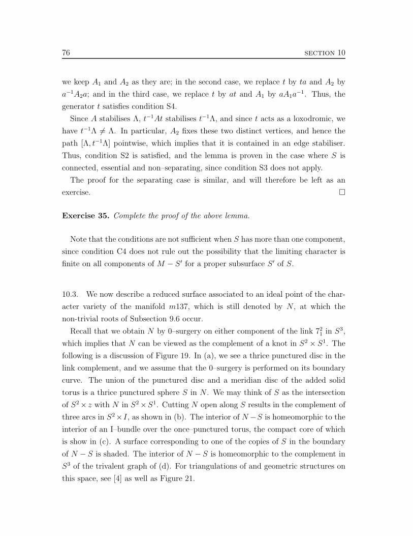
76 section 10
we keep A1 and A2 as they are; in the second case, we replace t by ta and A2 by
a−1A2a; and in the third case, we replace t by at and A1 by aA1a−1. Thus, the
generator t satisfies condition S4.
Since A stabilises Λ, t−1At stabilises t−1Λ, and since t acts as a loxodromic, we
have t−1Λ 6= Λ. In particular, A2 fixes these two distinct vertices, and hence the
path [Λ, t−1Λ] pointwise, which implies that it is contained in an edge stabiliser.
Thus, condition S2 is satisfied, and the lemma is proven in the case where S is
connected, essential and non–separating, since condition S3 does not apply.
The proof for the separating case is similar, and will therefore be left as an
exercise. �
Exercise 35. Complete the proof of the above lemma.
Note that the conditions are not sufficient when S has more than one component,
since condition C4 does not rule out the possibility that the limiting character is
finite on all components of M − S ′ for a proper subsurface S ′ of S.
10.3. We now describe a reduced surface associated to an ideal point of the char-
acter variety of the manifold m137, which is still denoted by N , at which the
non-trivial roots of Subsection 9.6 occur.
Recall that we obtain N by 0–surgery on either component of the link 721 in S3,
which implies that N can be viewed as the complement of a knot in S2 × S1. The
following is a discussion of Figure 19. In (a), we see a thrice punctured disc in the
link complement, and we assume that the 0–surgery is performed on its boundary
curve. The union of the punctured disc and a meridian disc of the added solid
torus is a thrice punctured sphere S in N . We may think of S as the intersection
of S2 × z with N in S2 ×S1. Cutting N open along S results in the complement of
three arcs in S2×I, as shown in (b). The interior of N−S is homeomorphic to the
interior of an I–bundle over the once–punctured torus, the compact core of which
is show in (c). A surface corresponding to one of the copies of S in the boundary
of N − S is shaded. The interior of N − S is homeomorphic to the complement in
S3 of the trivalent graph of (d). For triangulations of and geometric structures on
this space, see [4] as well as Figure 21.
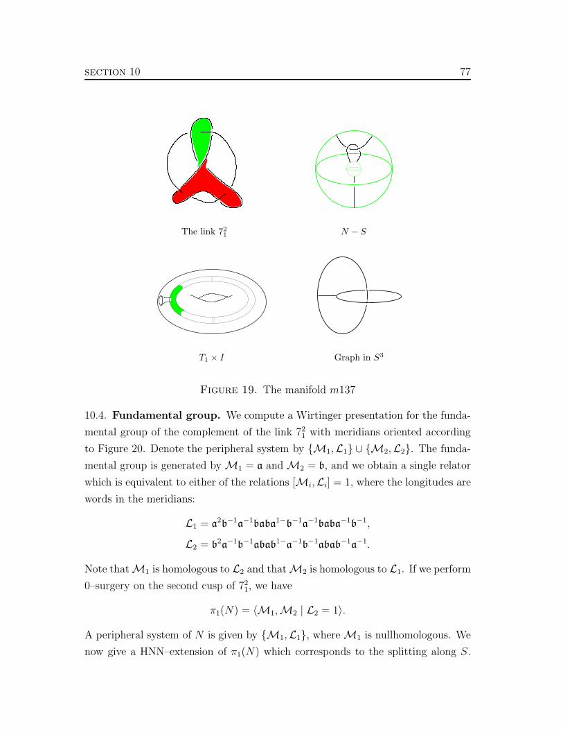
section 10 77
The link 72
1N − S
T1 × I Graph in S3
Figure 19. The manifold m137
10.4. Fundamental group. We compute a Wirtinger presentation for the funda-
mental group of the complement of the link 721 with meridians oriented according
to Figure 20. Denote the peripheral system by {M1,L1} ∪ {M2,L2}. The funda-
mental group is generated by M1 = a and M2 = b, and we obtain a single relator
which is equivalent to either of the relations [Mi,Li] = 1, where the longitudes are
words in the meridians:
L1 = a2b−1a−1baba1−b−1a−1baba−1b−1,
L2 = b2a−1b−1abab1−a−1b−1abab−1a−1.
Note that M1 is homologous to L2 and that M2 is homologous to L1. If we perform
0–surgery on the second cusp of 721, we have
π1(N) = 〈M1,M2 | L2 = 1〉.
A peripheral system of N is given by {M1,L1}, where M1 is nullhomologous. We
now give a HNN–extension of π1(N) which corresponds to the splitting along S.

78 section 10
F
M1
M2
π1(N)
G
M1
π1(S)
F M1
π1(N − S)
Figure 20. Generators for m137
It can be observed from Figure 20, that the elements M1 and F correspond to
generators of im(π1(N − S) → π1(N)), and if S− and S+ are the two copies of S
in ∂(N − S), then M1 ∈ im(π1(S−) → π1(N)) implies F ∈ im(π1(S+) → π1(N)).
Let
F = bab−1, G = F−1a−1Fa, H = F−1aFa−1,
and A = 〈a, F 〉, A1 = 〈a, G〉, A2 = 〈F,H〉.
Each of the groups A, A1 and A2 is free in two generators, and π1(N) is an HNN–
extension of A across A1 and A2 by M2 = b with the relations
bab−1 = F, bGb−1 = HF.
This HNN–extension corresponds to the splitting of N along S.
section 10 79
10.5. Representation spaces. With the method of Subsection 4.7, irreducible
representations of N can (up to conjugation and birational equivalence) be param-
eterised by:
ρ(a) =
(
m 0(1−m)(b2(m2−1)−m)
b2(m−1)+m2+m3 m−1
)
, ρ(F ) =
(
m 1
0 m−1
)
ρ(b) =
(
b2(1−m)+b4(1−m)2−m2
b(m−1)(b2(m−1)+m2+m3)b
b(1−m)(b2(m2−1)−m)b2(m−1)+m2+m3 b(m−1 −m)
)
,
subject to
0 = m3(1 +m+m2)
+ b2m(m2 − 1)(1 −m+m2 + 2m4 +m5) − b4(m− 1)2(1 +m+m2).
Thus, as b → 0, we observe that either m → 0 or m tends to a non–trivial third
root of unity, which we denote by ζ3. Since
tr ρ(b) =−m4 − b2m3(1 −m)2 + b4(1 −m)2
bm(m− 1)(b2(m− 1) +m2 +m3),
it follows that as b→ 0 and m→ ζ3, we have tr ρ(b) → ∞, and an ideal point ξ of
the character variety is approached. Moreover, the A–polynomial can be computed
from the above, and we obtain:
0 = (m13 − l4)(1 −m)(1 +m+m2)3
− l2m3(1 +m2)(1 + 3m+m2 − 2m3 − 3m4 − 2m5 + 2m6
− 2m7 − 3m8 − 2m9 +m10 + 3m11 +m12).
As m → ζ3, we have l → 0, and hence tr ρ(L1) → ∞. Thus, M1 is a strongly
detected boundary slope associated to ξ. The limiting representations of the images
of A, A1 and A2 in π1(N) are determined by:
tr ρ(a) → −1, tr ρ(F ) → −1, tr ρ(Fa) → −ζ3, tr ρ[a, F ] → −1,
tr ρ(a) → −1, tr ρ(G) → −1, tr ρ(Ga−1) → −1, tr ρ[a, G] → 2,
tr ρ(F ) → −1, tr ρ(H) → −1, tr ρ(FH) → −1, tr ρ[F,H ] → 2.
Thus, the limiting representation is irreducible on A, and reducible on A1 and
A2. Since both tr ρ(b) and tr ρ(L1) blow up, Lemma 39 implies that S is a reduced
associated surface.

80 section 10
2π3
2π3
2π3
2π3
2π3
π3
π3
Figure 21. To obtain the limiting orbifold, first glue the faces meeting
along one of the edges with cone angle 2π/3 to obtain a spindle, and then
identify the boundary discs of the spindle. The result is S3 minus two
points, with the labelled graph (minus its vertices) as the singular locus.
Exercise 36. There are two thrice punctured discs in the complement of the link
721, one of which has boundary slopes determined by the pair (L2,M1), the other
by the pair (L1,M2). Denote these discs by D1 and D2 respectively. We observed
that the boundary components of each of these discs are homologous, and that 0
Dehn filling on the second cusp lets D1 descend to a properly embedded surface in
N , which we have associated to the slope 0.
The disc D2 descends to a surface in N which is not properly embedded since the
boundary curve M2 is not peripheral. However, the slope ∞ determined by L1 is
detected by the reducible representations of π1(N). Can you modify D2 and detect
the resulting (essential) surface?
10.6. Degeneration of the hyperbolic structure. Since the limiting eigenvalue
is a third root of unity, the limiting representation may correspond to a geometric
decomposition of the orbifold N(3, 0). Using SnapPea, we can observe the defor-
mation of the ideal triangulation of N as we approach N(3, 0). The manifold m137
has a triangulation with four tetrahedra, and as we approach N(3, 0) through pos-
itively oriented triangulations determined by the surgery coefficients (p, 0) with
p ≥ 3, three tetrahedra degenerate, whilst the remaining tetrahedron has limiting
shape parameter 12
+√
36i. In fact, N(3, 0) contains a Euclidean (3, 3, 3)–turnover
whose complement is a hyperbolic 3–orbifold of volume approximately 0.68 which
can be triangulated by a single ideal tetrahedron as shown in Figure 21. Note that
the link of each vertex of the tetrahedron is a Euclidean (3, 3, 3)–turnover.

section 10 81
References
[1] Alperin and Shalen: Linear groups of finite cohomological dimension, Invent. Math., 66,
89-98, (1982).
[2] G. Baumslag: Topics in Combinatorial Group Theory, Birkhauser, Basel Boston Berlin,
1993.
[3] G.M. Bergman: A weak Nullstellensatz for valuations, Proc. Amer. Math. Soc., 28, 32-38
(1971).
[4] M. Boileau and J. Porti, Geometrization of 3-orbifolds of cyclic type, Appendix A by M.
Heusener and Porti. Asterisque No. 272, 2001.
[5] S.Boyer, X.Zhang: On Culler–Shalen seminorms and Dehn filling, Ann. Math., 148, 737-801
(1998).
[6] Gerhard Burde, Heiner Zieschang: Knots, de Gruyter, 1985.
[7] D. Cooper, M. Culler, H. Gillett, D.D. Long and P.B. Shalen: Plane curves associated to
character varieties of 3–manifolds, Invent. Math., 118, 47-84 (1994).
[8] D. Cooper, C.D. Hodgson, S.P. Kerckhoff: Three–dimensional Orbifolds and Cone–
Manifolds, MSJ Memoir 5, Tokyo, 2000.
[9] D. Cooper, D.D. Long: Remarks on the A-polynomial of a Knot, J. Knot Theory Ramifica-
tions, 5, 609-628 (1996).
[10] D. Cooper, D.D. Long: Representation Theory and the A-polynomial of a knot, Chaos,
Solitions & Fractals, 9, 749-763 (1998).
[11] D. Cooper, D.D. Long: The A–polynomial has ones in the corners, Bull. London Math. Soc.,
29, 2, 231–238 (1997).
[12] David Cox, John Little, Donal O’Shea: Ideals, Varieties, and Algorithms, Springer Verlag,
New York, 1992.
[13] Marc Culler, C.McA. Gordon, J. Luecke, Peter B.Shalen: Dehn surgery on knots, Ann.
Math., 125, 237-300 (1987).
[14] Marc Culler, Peter B. Shalen: Varieties of group representations and splittings of 3-
manifolds, Ann. Math., 117, 109-146 (1983).
[15] Nathan M. Dunfield: Examples of non-trivial roots of unity at ideal points of hyperbolic
3-manifolds, Topology, 38, 457-465 (1999).
[16] Nathan M. Dunfield: Cyclic Surgery, degrees of maps of character curves, and volume rigidity
for hyperbolic manifolds, Invent. Math., 136, 623-657 (1999).
[17] F. Gonzalez-Acuna, J.M. Montesinos-Amilibia: On the character variety of group presenta-
tions in SL2(C) and PSL2(C), Math. Z. 214, 626-652 (1993).
[18] O. Goodman, C.D. Hodgson, W.D. Neumann: Snap, Tube, Isometric, available from
http://www.ms.unimelb.edu.au/∼snap.
[19] John Hempel: 3–manifolds, Princeton University Press, Princeton, 1976.
[20] D.D. Long, A.W. Reid: Commensurability and the character variety, preprint, 1999.
82 section 10
[21] W.S.Massey: Algebraic Topology: An Introduction, Springer Verlag, New York, 1967.
[22] James R.Munkres: Elements of Algebraic Topology.
[23] Walter D.Neumann: Notes on Geometry and 3–manifolds, Low Dimensional Topology,
Boroczky, Neumann, Stipsicz, Eds., Bolyai Society Mathematical Studies 8 (1999), 191–267.
[24] H.Seifert, W.Threlfall: A textbook of topology, Academic press, New York, 1980.
[25] J.–P. Serre: Trees, Springer, Berlin, 1980.
[26] Igor R.Shafarevich: Basic Algebraic Geometry 1 & 2, Springer Verlag, Berlin, 1994.
[27] Peter B.Shalen: Representations of 3–manifold groups, Handbook of geometric topology,
955-1044, Amsterdam, 2002.
[28] Peter B.Shalen: Three–manifold topology and the tree for PSL2, Cont. Math., 243, 189-209
(1999).
[29] Edwin H.Spanier: Algebraic Topology, McGraw-Hill, New York, 1966.
[30] W.P. Thurston: The geometry and topology of 3–manifolds, Princeton Univ. Math. Dept.
(1978). Available from http://msri.org/publications/books/gt3m/.
[31] W. Thurston: Three Dimensional Geometry, Princeton University Press, Princeton, 1983.
[32] S. Tillmann: Character varieties of mutative 3–manifolds, math.GT/0306053.
[33] S. Tillmann: Boundary slopes and the logarithmic limit set, math.GT/0306055.
[34] J.R. Weeks: SnapPea available from http://www.geometrygames.org/SnapPea/.
Current address: Department de mathematiques, Universite du Quebec a Montreal,
Case postale 8888, succursale Centre-Ville, Montreal (Quebec) Canada H3C 3P8.