finding the relationship between elevation and isotopic ... · finding the relationship between...
TRANSCRIPT

Derry Xu Drx55 (GEO 327G)
Finding the Relationship Between Elevation and Isotopic Compositions of Stream Waters in the Peruvian Andes
Abstract
The Peruvian Andes is a prime example of highly-elevated topography generated by oceanic
plate subduction. As a result, several studies have been made to further understand the formation of
the Andean Mountain Range, but as indicated by previous studies (Schildgen et al, 2007), researchers
are still unable to ascertain the of the magnitude of the uplift solely based on structural history due to
conflicting uplift histories and tectonic drivers. Several (conflicting) geodynamic theories and models
were suggested for explaining the Andean orogeny— one of which was a continuous late Cenozoic event
that caused the delamination of the lithosphere on the South American plate, which in turn generated
plate uplift and canyon incisions in the late Miocene. Another theory was that during the late Cenozoic,
the crust continuously thickened and shortened, which resulted in slow surface uplift and also caused
canyon incision. As a result, we believe that best way to confirm or dis-prove the currently proposed
models would be to apply several different proxy approaches that deviate from structural history
research while extending the research areas in question.
To accomplish this, Dr. Breecker and his research group will combine proxy approaches, which
involve retrieving volcanic glasses and soil carbonates to analyze and perform stable isotope analyses for
δD values, while analyzing ignimbrites using the 40Ar/39Ar geochronometer (these studies are to be
done by another professor off campus in the research group). This is to be performed in conjunction
with the analysis of a general circulation climate model (Poulsen et al 2007) that approximates the scale
of the surface elevation changes and their effects on climate (Poulsen et al 2010)— to further verify the
general circulation climate models, modern waters in the region can be analyzed using soil collection
techniques (that undergo water extraction) along with precipitation gauge and rain bucket data. Field
collection is a necessary process because there are no published data on the soil, precipitation, or

Derry Xu Drx55 (GEO 327G)
stream water values on the study region, (there are few precipitation stations in Peru, but not enough to
accurately model precipitation isotopic values).
IEGCMs, or isotope-enabled atmospheric general circulation models, are used to quantify
regional (Fig. 3) and global climate change, allowing the distortion of isotope values (δ 18O, D) to be
recognized (Poulsen 2010). As a result, the usage is IEGCMs is vital in our volcanic glass and soil
carbonate analyses, as we want to minimize the external effects on the δ 18O or δ D values. The δ D
value is especially important to determine because through δ D records, one can determine the
elevation at which a measurement was taken, as higher elevations correlate with lower δ D values. This
inverse relationship occurs because of the rain off effect; when rain occurs in a region of increasing
elevations, water that is δ D enriched is deposited first at lower elevations, whereas δ 18O enriched
precipitation is deposited more towards the peaks in elevation, and the leeward side of the peak usually
receives less water overall (unless multi-directional winds are experienced due to a phenomenon like El
Ninõ, in which that complicates analysis).
One large assumption is made when using these two coupled IECGMs, the assumption that the
IECGMs perform correctly under the scenario of this project. To further evaluate these models on their
ability to quantify all extraneous factors affecting the δ 18O or δ D values, our research group plans to
sample and analyze river waters (or waters extracted from soils) from Peru—the physical results can be
compared to the IECGMs’ modeled results, possibly revealing insight about the limitations of these
models (if there are any). This is a necessary process because there is currently no publication data on
the soil, precipitation, or stream water values on the study region, (there are few precipitation stations
in Peru, but not enough to accurately model precipitation isotopic values).
Purpose

Derry Xu Drx55 (GEO 327G)
As a result, making a map of the analyzed river waters can be an essential step to the formation
of this research paper—maps of the sampled river waters not only provide a visual for the sampling
locations, but it also brings the ability to spatially analyze the collected stream waters, bringing
important relationships to light such as the correspondence between elevation and isotopic
compositions of sampled waters. By calculating the area of upstream drainage basins for each sample
point, one can split the basin areas of each sample into elevation ranges (~200m, 500m, etc.). After
partitioning all of the drainage basin areas into groups, the weighted mean elevation for stream water
can be calculated, and using the isotopic composition data provided by the research group in Peru, one
can finally determine the relationship between isotopic composition and elevation, and see whether or
not the coupled IECGMs also follow this relationship in its modeling process.
Due to the huge data load from ASTER DEMs and the instability of arcMap when handling large
amounts of raster data, a “Proof of Concept” was established for the purposes of this class—instead of
using all 26 of the sampling locations, which span over 15 ASTER DEMs (provided by NASA Reverb), only
one sample location will be used (labled R120) due to its easy-to-spot general basin drainage area and
its lack of nearby sample points (to reduce clutter). This “Proof of Concept” will also help the user learn
the skills necessary to operate ArcHydro tools in ArcMap (which were never explicitly used in class),
while combining preexisting skills learned from GEO327G. Because the “Proof of Concept” only has one
point, the weighted mean elevation of all stream water samples is not necessary because there is only
one stream sample focused on in this (the POC).
Data gathering and Pre-Processing
Because of the Peruvian government did not provide a free DEM for the country, individual files
from the ASTER GDEM had to be ordered and downloaded. The streams and inland waters were
displayed from files by DIVA-GIS—while the files are not from a governmental organization, the data

Derry Xu Drx55 (GEO 327G)
matches up relatively well with the DEMs, and DIVA-GIS was created by Robert J. Jijmans, a professor at
UC Davis. A lot of preprocessing was required for any of the data was to be used—the sampled river
data obtained by the research team in Peru was listed in UTM Eastings and Northings. The ASTER DEM
data used GCS_WGS_1984, along with the inland water data. The preferred coordinate system for this
project was South America Albers Equal Area Conic (which uses the South American 1969 datum). As a
result, the sample location data points had to be imported as UTM coordinates to arcMap using the
“Excel to Table” tool. Then, the points had to be projected (and saved as layer file) to the South America
Albers Equal Area Conic, along with adding all the other files downloaded. ESRI Basemaps were then
added to fill the blankness of the map region. After this somewhat tenuous process, the method could
then be conducted.

Derry Xu Drx55 (GEO 327G)
Map 1- Post Preprocessing Map with a general view of the study area.

Derry Xu Drx55 (GEO 327G)
Method*
*tools or processes already performed in labs will not have supplementary photos. Spatial Analyst and 3D Analyst were turned on beforehand.
After all data processing was conducted, the first step was to create a mosaic for the area of interest (using the “Create a Mosaic Dataset” tool). This can be seen with Map 2. A “Fill” was also conducted to the mosaic to fix any errors due to the resolution of the data or rounding of elevations to the nearest integer value.
Map 2—Outlining the study areas for the POC. Two DEMs were used to test and review the mosaic process, even though DEM S6_W73 is not necessary.
Derry Xu Drx55 (GEO 327G)
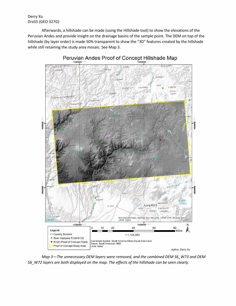
Afterwards, a hillshade can be made (using the Hillshade tool) to show the elevations of the Peruvian Andes and provide insight on the drainage basins of the sample point. The DEM on top of the hillshade (by layer order) is made 50% transparent to show the “3D” features created by the hillshade while still retaining the study area mosaic. See Map 3.
Map 3—The unnecessary DEM layers were removed, and the combined DEM S6_W73 and DEM S6_W72 layers are both displayed on the map. The effects of the hillshade can be seen clearly.
Derry Xu Drx55 (GEO 327G)
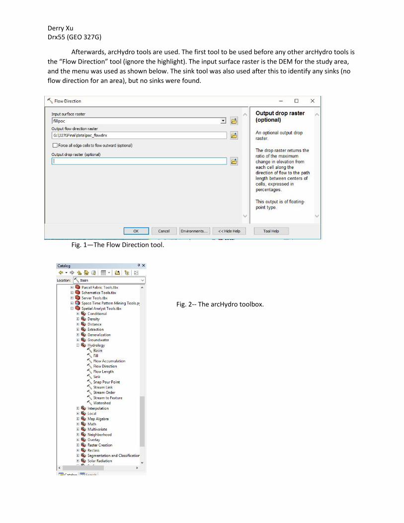
Afterwards, arcHydro tools are used. The first tool to be used before any other arcHydro tools is the “Flow Direction” tool (ignore the highlight). The input surface raster is the DEM for the study area, and the menu was used as shown below. The sink tool was also used after this to identify any sinks (no flow direction for an area), but no sinks were found.
Fig. 1—The Flow Direction tool.
Fig. 2-- The arcHydro toolbox.

Derry Xu Drx55 (GEO 327G)
Fig 3—The Sink tool. It had no effect for this map because no sinks were made, and thus could not be corrected.
Fig. 4—The result of the flow direction raster. Every cell is assigned a direction for water flow due to the changes in elevation from cell to cell.
Afterwards, the watershed tool could be used. The input raster was the flow direction raster, the point of the interest was the POC, and the watershed was to be determined by the “Elevation” field of the point.

Derry Xu Drx55 (GEO 327G)
Fig 5 – Watershed tool. Output raster is not actually in that place.

Derry Xu Drx55 (GEO 327G)
Map 4—Drainage Basin. The Peruvian inland water sources and rivers are added to this map.
(The label for the drainage basin is missing on this map, note.).
Derry Xu Drx55 (GEO 327G)
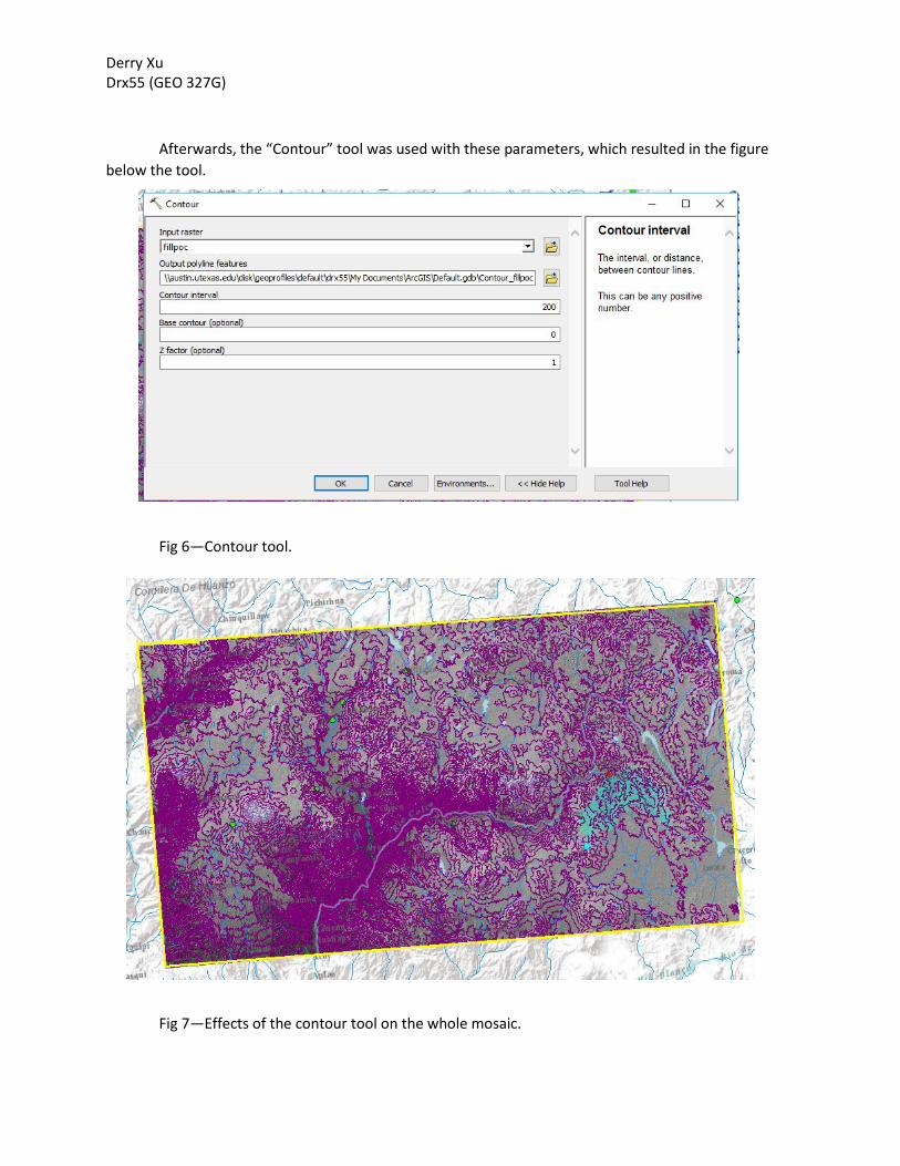
Afterwards, the “Contour” tool was used with these parameters, which resulted in the figure below the tool.
Fig 6—Contour tool.
Fig 7—Effects of the contour tool on the whole mosaic.
Derry Xu Drx55 (GEO 327G)
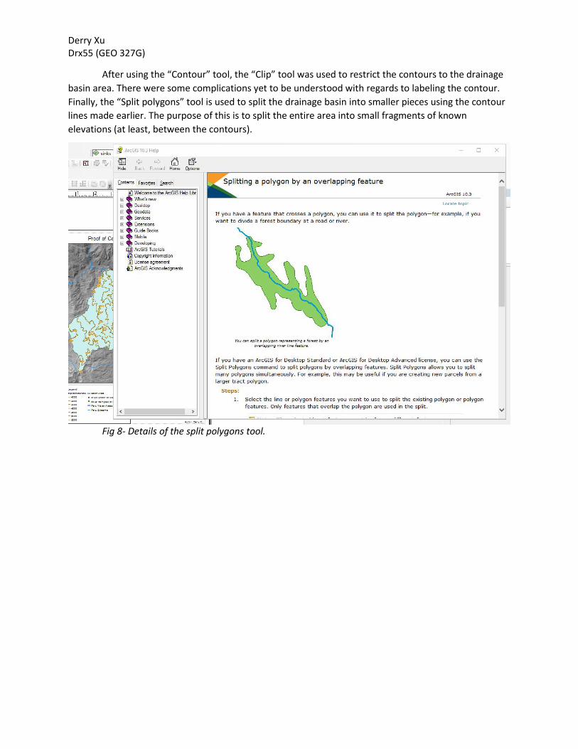
After using the “Contour” tool, the “Clip” tool was used to restrict the contours to the drainage basin area. There were some complications yet to be understood with regards to labeling the contour. Finally, the “Split polygons” tool is used to split the drainage basin into smaller pieces using the contour lines made earlier. The purpose of this is to split the entire area into small fragments of known elevations (at least, between the contours).
Fig 8- Details of the split polygons tool.

Derry Xu Drx55 (GEO 327G)
Map 5- The final POC Map of the drainage Basin. The “jigsaw” Basin Area layer cannot be seen, but it can be viewed via the attribute table. The area of each portion is also calculated. (See Fig 9).

Derry Xu Drx55 (GEO 327G)
Fig 9- Proof that the basin is now split into smaller pieces, each labeled with areas.

Derry Xu Drx55 (GEO 327G)
Conclusion
As a result of all the data collection, a spreadsheet (Fig 10) of all the areas of each “piece” of the
basin bounded by elevation contours of 200m is formed (“Table to Spreadsheet” was used to export the
data). Using this data, one can find the area of each portion, match it to the corresponding contours it is
bound by, and eventually obtain the weight of each 200m section detailed by the data. Of course, this
requires a lot of tedious, rote Excel processing, and for the sake of this assignment, the concept is more
important. Once the Excel operations are performed, the data for the POC can be correlated to a
spreadsheet of all the isotopic compositions for the samples (measured vs. SMOW), (Fig 11). As said
referenced earlier, this entire process is to be repeated 25 more times so that each point can calculate
the area of its drainage basin with respect to its elevation. Even though this entire process is extremely
tedious, the end process can be worthwhile, for only using arcMap, physically sampled river samples,
and an assortment of data collected from the internet, one can essentially “peer-review” (or at the least
cast doubt) on some frequently used climate models.

Derry Xu Drx55 (GEO 327G)
Fig 10- Exported Areas of all the pieces of the drainage basin.

Derry Xu Drx55 (GEO 327G)
Fig 11- Isotopic Values, R120 is highlighted.
Derry Xu Drx55 (GEO 327G)
Sources:
(Tutorial for arcHydro)
https://www.crwr.utexas.edu/gis/gishydro07/Introduction/Exercises/Ex4.html
Rivers Peru
http://www.diva-gis.org/gdata
Peru GDEM
https://reverb.echo.nasa.gov/reverb/orders/B9FAD62A-923B-8496-88CB-F01DE33BA7C7/submit
Works Cited
Poulsen, C. J., Pollard, D., and White, T. S., 2007, General circulation model simulation of the δ18O content of continental precipitation in the middle Cretaceous: A model-proxy comparison: Geology, v. 35, no. 3, p. 199-202.
Poulsen, C. J., Ehlers, T. A., and Insel, N., 2010, Onset of Convective Rainfall During Gradual Late Miocene Rise of the Central Andes: Science, v. 328, p. 490-493.
Schildgen, T. F., Hodges, K. V., Whipple, K. X., Reiners, P. W., and Pringle, M. S., 2007, Uplift of the western margin of the Andean plateau revealed from canyon incision history, southern Peru: Geology, v. 35, no. 6, p. 523-526.