finding the right words - birot.hu · finding the right words implementing optimality theory with...
TRANSCRIPT
Finding the Right WordsImplementing Optimality Theory
with Simulated Annealing
Tamas Bıro
Work presented developed at:Humanities Computing
CLCGUniversity of Groningen
Present affiliation:Theoretical Linguistics
ACLCUniversity of Amsterdam
Amsterdam, ILLC, March 2, 2007
Tamas Bıro 1/ 33

Overview
• Optimality Theory (OT) in a nutshell
• Simulated Annealing for Optimality Theory (SA-OT)
• Examples
• The dis-harmonic mind?
• Conclusion
Tamas Bıro 2/ 33

Optimality Theory in a nutshell
OT tableau: search the best candidate w.r.t lexicographic ordering
(cf. abacus, abolish,..., apple,..., zebra)
cn cn−1 ... ck+1 ck ck−1 ck−2 ...
w 2 0 1 2 3 0
w’ 2 0 1 3 ! 1 2
w” 3 ! 0 1 3 1 2
Tamas Bıro 3/ 33

Optimality Theory in a nutshell
• Pipe-line vs. optimize the Eval-function
• Gen: UR 7→ {w|w is a candidate corresponding to UR}
E.g. assigning Dutch metrical foot structure & stress:
fototoestel 7→ {fototoe(stel), (foto)(toestel), (fo)to(toestel),...}
Tamas Bıro 4/ 33

Optimality Theory: an optimization problem
UR 7→ {w|w is a candidate corresponding to UR}E(w) =
(CN(w), CN−1(w), ..., C0(w)
)∈ NN+1
0
SR(UR) = argoptw∈Gen(UR)E(w)
Optimization: with respect to lexicographic ordering
Tamas Bıro 5/ 33

OT is an optimization problem
The question is:How can the optimal candidate be found?
• Finite-State OT (Ellison, Eisner, Karttunen, Frank & Satta, Gerdemann &
van Noord, Jager...)
• chart parsing (dynamic programming) (Tesar & Smolensky; Kuhn)
These are perfect for language technology. But we would like apsychologically adequate model of linguistic performance (e.g.errors): Simulated Annealing.
Tamas Bıro 6/ 33

How to find optimum: Gradient Descent 1
w := w_init ;Repeat
w’:= best element of set Neighbours(w);Delta := E(w’) - E(w) ;if Delta < 0 then w := w’ ;else
do nothing
end-if
Until stopping condition = true
Return w # w is an approximation to the optimal solution
Tamas Bıro 7/ 33

How to find optimum: Gradient Descent 2
w := w_init ;Repeat
Randomly select w’ from the set Neighbours(w);Delta := E(w’) - E(w) ;if Delta < 0 then w := w’ ;else
do nothing
end-if
Until stopping condition = true
Return w # w is an approximation to the optimal solution
Tamas Bıro 8/ 33
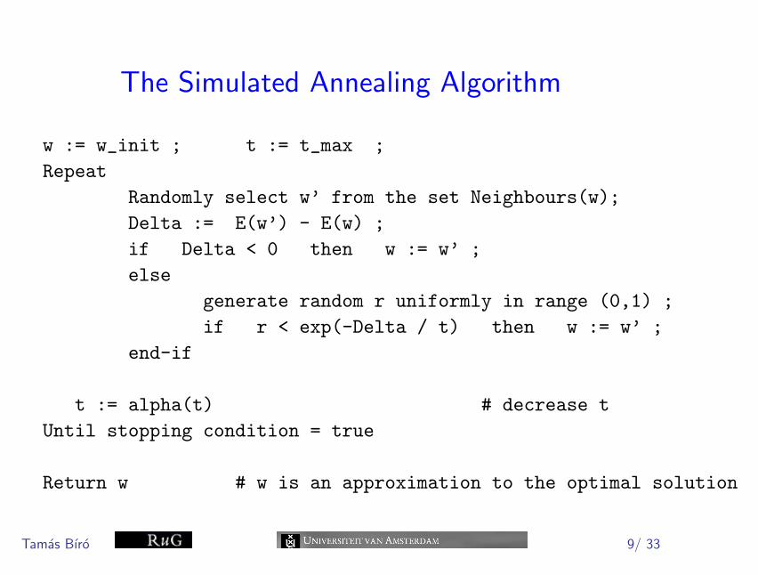
The Simulated Annealing Algorithm
w := w_init ; t := t_max ;Repeat
Randomly select w’ from the set Neighbours(w);Delta := E(w’) - E(w) ;if Delta < 0 then w := w’ ;else
generate random r uniformly in range (0,1) ;if r < exp(-Delta / t) then w := w’ ;
end-if
t := alpha(t) # decrease tUntil stopping condition = true
Return w # w is an approximation to the optimal solution
Tamas Bıro 9/ 33
Deterministic Gradient Descent for OT
• McCarthy (2006): persistent OT (harmonic serialism, cf.Black 1993, McCarthy 2000, Norton 2003).
• Based on a remark by Prince and Smolensky (1993/2004) ona “restraint of analysis” as opposed to “freedom of analysis”.
• Restricted Gen → Eval → Gen → Eval →... (n times).
• Gradual progress toward (locally) max. harmony.
• Employed to simulate traditional derivations, opacity.
Tamas Bıro 10/ 33
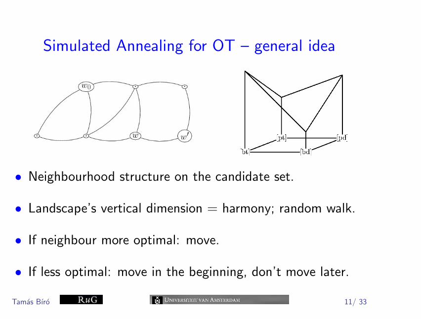
Simulated Annealing for OT – general idea
• Neighbourhood structure on the candidate set.
• Landscape’s vertical dimension = harmony; random walk.
• If neighbour more optimal: move.
• If less optimal: move in the beginning, don’t move later.
Tamas Bıro 11/ 33

Simulated Annealing for OT – general idea
• Neighbourhood structure → local optima.
• System can get stuck in local optima: alternation forms.
• Precision of the algorithm depends on its speed (!!).
• Many different scenarios.
Tamas Bıro 12/ 33

Sim. annealing with non-real valued target function
• Exponential weights if upper bound on Ci(w) violation levels:
E(w) = CN(w)·qN+CN−1(w)·qN−1+...+C1(w)·q+C0(w)
• Polynomials:
E(w)[q] = CN(w)·qN+CN−1(w)·qN−1+...+C1(w)·q+C0(w)
• Ordinal weights:
E(w) = ωNCN(w) + ... + ωC1(w) + C0(w)
Tamas Bıro 13/ 33

Sim. annealing with non-real valued target function
Transition probability if w′ worse than w: what is eE(w′)−E(w)
t ?
• Polynomials:
T [q] = 〈KT , t〉 [q] = t · qKT
P(w → w′ ∣∣ T [q]
)= lim
q→+∞e−E(w′)[q]−E(w)[q]
T [q]
• Ordinals: move iff the generated r ∈ [0, 1] is s.t.
∀α ∈ N+ : r−α > 2q
(∆(E(w′),E(w)
)·α,T
)Tamas Bıro 14/ 33

Domains for temperature and constraints
• Temperature: T = 〈KT , t〉 ∈ Z× R+ (or “Z”×R+).
• Constraints associated with domains of KT :
– – C0 C1 C2
. . . K = −1 K = 0 K = 1 K = 2 . . .
. . . ... 0.5 1.0 1.5 2.0 2.5 ... 0.5 1.0 1.5 2.0 2.5 ... 0.5 1.0 1.5 2.0 2.5 ... 0.5 1.0 1.5 2.0 2.5 . . .
Tamas Bıro 15/ 33

Rules of moving
Rules of moving from w to w′
at temperature T = 〈KT , t〉:
If w′ is better than w: move! P (w → w′|T ) = 1
If w′ loses due to fatal constraint Ck:
If k > KT : don’t move! P (w → w′|T ) = 0
If k < KT : move! P (w → w′|T ) = 1
If k = KT : move with probability
P = e−(Ck(w′)−Ck(w))/t
Tamas Bıro 16/ 33

The SA-OT algorithm
w := w_init ;for K = K_max to K_min step K_step
for t = t_max to t_min step t_stepCHOOSE random w’ in neighbourhood(w) ;COMPARE w’ to w: C := fatal constraint
d := C(w’) - C(w);if d <= 0 then w := w’;else w := w’ with probability
P(C,d;K,t) = 1 , if C < K= exp(-d/t) , if C = K= 0 , if C > K
end-forend-forreturn w
Tamas Bıro 17/ 33
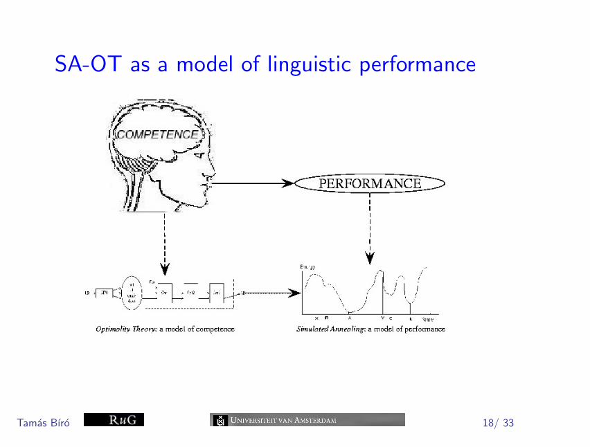
SA-OT as a model of linguistic performance
Tamas Bıro 18/ 33

Proposal: three levels
Level its product its model the product
in the model
Competence in narrow standard globally
sense: static knowledge grammatical form OT optimal
of the language grammar candidate
Dynamic language acceptable or SA-OT local
production process attested forms algorithm optima
Performance in its acoustic (phonetics,
outmost sense signal, etc. pragmatics) ??
Tamas Bıro 19/ 33
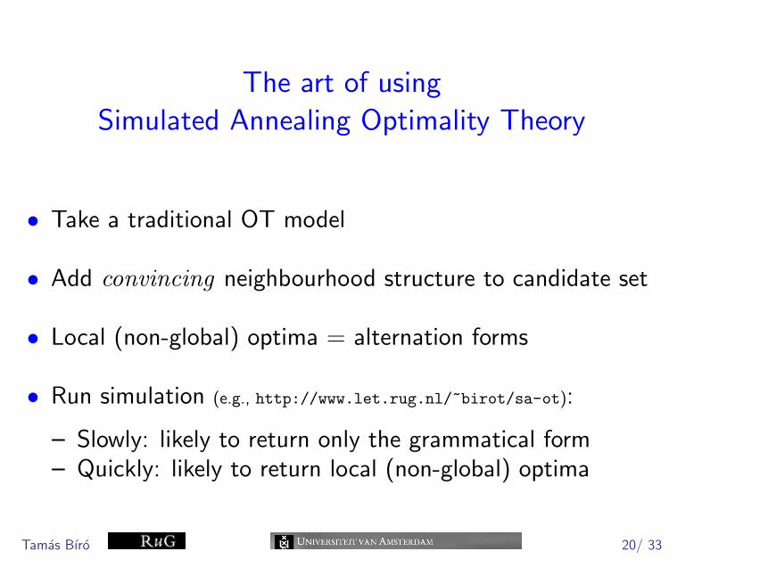
The art of using
Simulated Annealing Optimality Theory
• Take a traditional OT model
• Add convincing neighbourhood structure to candidate set
• Local (non-global) optima = alternation forms
• Run simulation (e.g., http://www.let.rug.nl/~birot/sa-ot):
– Slowly: likely to return only the grammatical form– Quickly: likely to return local (non-global) optima
Tamas Bıro 20/ 33

Parameters of the algorithm
• tstep (and tmax, tmin)
• Kmax (and Kmin)
• Kstep
• w0 (inital candidate)
• Topology (neighbourhood structure)
• Constraint hierarchy
Tamas Bıro 21/ 33
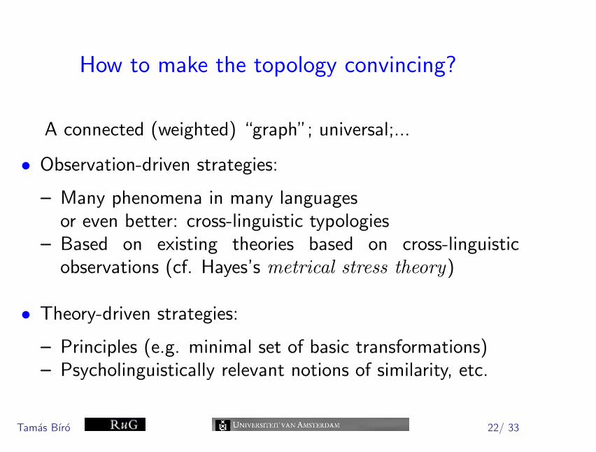
How to make the topology convincing?
A connected (weighted) “graph”; universal;...
• Observation-driven strategies:
– Many phenomena in many languagesor even better: cross-linguistic typologies
– Based on existing theories based on cross-linguisticobservations (cf. Hayes’s metrical stress theory)
• Theory-driven strategies:
– Principles (e.g. minimal set of basic transformations)– Psycholinguistically relevant notions of similarity, etc.
Tamas Bıro 22/ 33

Example: Fast speech: Dutch metrical stress
fo.to.toe.stel uit.ge.ve.rij stu.die.toe.la.ge per.fec.tio.nist‘camera’ ‘publisher’ ‘study grant’ ‘perfectionist’
susu ssus susuu usus
fo.to.toe.stel uit.ge.ve.rıj stu.die.toe.la.ge per.fec.tio.nıstfast: 0.82 fast: 0.65 / 0.67 fast: 0.55 / 0.38 fast: 0.49 / 0.13slow: 1.00 slow: 0.97 / 0.96 slow: 0.96 / 0.81 slow: 0.91 / 0.20
fo.to.toe.stel uit.ge.ve.rıj stu.die.toe.la.ge per.fec.tio.nıstfast: 0.18 fast: 0.35 / 0.33 fast: 0.45 / 0.62 fast: 0.39 / 0.87slow: 0.00 slow: 0.03 / 0.04 slow: 0.04 / 0.19 slow: 0.07 / 0.80
Simulated / observed (Schreuder) frequencies.
In the simulations, Tstep = 3 used for fast speech and Tstep = 0.1 for slow
speech.
Tamas Bıro 23/ 33
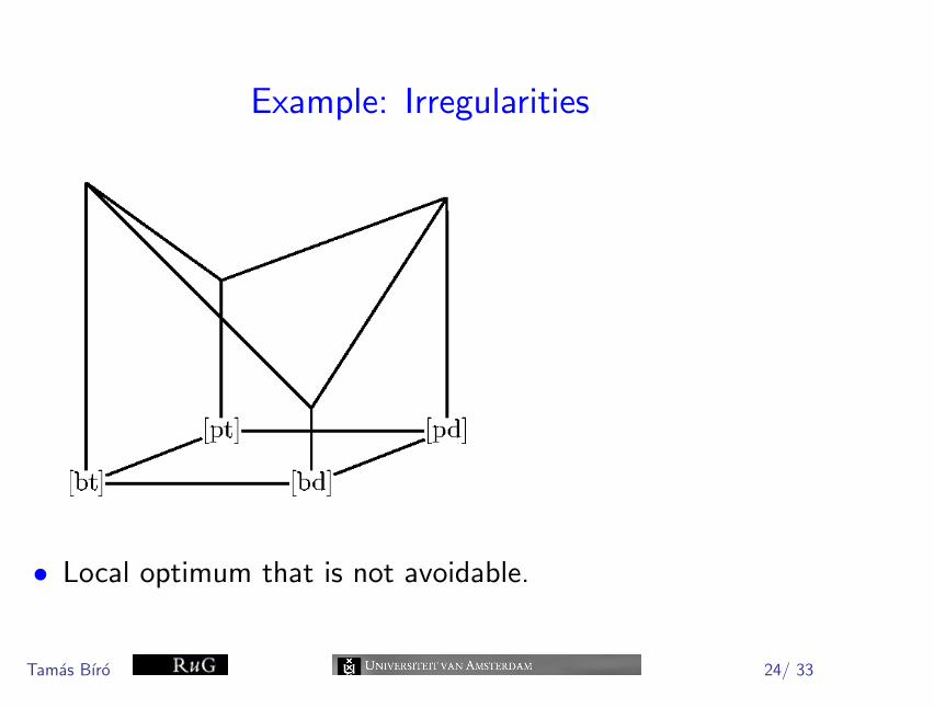
Example: Irregularities
• Local optimum that is not avoidable.
Tamas Bıro 24/ 33

Example: string-grammar
• Candidates: {0, 1, ..., P − 1}L
E.g. (L = P = 4): 0000, 0001, 0120, 0123,... 3333.
• Neighbourhood structure: w and w′ neighbours iff one basicstep transforms w to w′.
• Basic step: change exactly one character ±1, mod P(cyclicity).
• Each neighbour with equal probability.
Tamas Bıro 25/ 33

Example: string-grammar
Markedness Constraints (w = w0w1...wL−1, 0 ≤ n < P ):
• No-n: *n(w) :=∑L−1
i=0 (wi = n)
• No-initial-n: *Initialn(w) := (w0 = n)
• No-final-n: *Finaln(w) := (wL−1 = n)
• Assimilation Assim(w) :=∑L−2
i=0 (wi 6= wi+1)
• Dissimilation Dissim(w) :=∑L−2
i=0 (wi = wi+1)
Tamas Bıro 26/ 33
Example: string-grammar
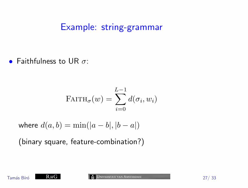
• Faithfulness to UR σ:
Faithσ(w) =L−1∑i=0
d(σi, wi)
where d(a, b) = min(|a− b|, |b− a|)
(binary square, feature-combination?)
Tamas Bıro 27/ 33
Example: string-grammar
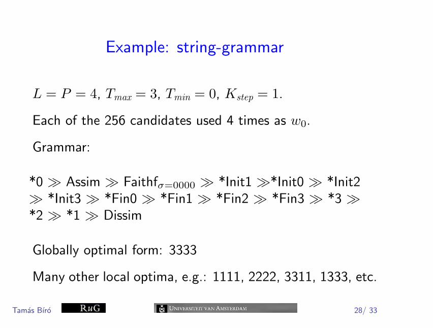
L = P = 4, Tmax = 3, Tmin = 0, Kstep = 1.
Each of the 256 candidates used 4 times as w0.
Grammar:
*0 � Assim � Faithfσ=0000 � *Init1 �*Init0 � *Init2� *Init3 � *Fin0 � *Fin1 � *Fin2 � *Fin3 � *3 �*2 � *1 � Dissim
Globally optimal form: 3333
Many other local optima, e.g.: 1111, 2222, 3311, 1333, etc.
Tamas Bıro 28/ 33

Example: string-grammar
Output frequencies for different Tstep values:
output 0.0003 0.001 0.003 0.01 0.03 0.1
1111 0.40 0.40 0.36 0.35 0.32 0.243333 0.39 0.39 0.41 0.36 0.34 0.212222 0.14 0.14 0.15 0.18 0.19 0.173311 0.04 0.04 0.04 0.05 0.06 0.051133 0.03 0.04 0.04 0.04 0.05 0.04others – – – – 0.04 0.29
Tamas Bıro 29/ 33

What does SA-OT offer to standard OT?
• A new approach to account for variation:
– Non-optimal candidates also produced (cf. Coetzee);– As opposed to: more candidates with same violation
profile; more hierarchies in a grammar.
• A topology (neighbourhood structure) on the candidate set.
• Additional ranking arguments (cf. McCarthy 2006) →learning algorithms (in progress).
• Arguments for including losers (never winning candidates).
Tamas Bıro 30/ 33

The dis-harmonic mind?
ICS (Integrated Connectionist/Symbolic Cognitive Architecture):
“[T]here is no symbolic algorithm whose internal structure can predict
the time and the accuracy of processing; this can only be done with
connectionist algorithms” (Smolensky and Legendre (2006): TheHarmonic Mind, vol. 1, p. 91).
SA-OT:
• symbolic computation only
• predicts tme and accuracy of processing
Tamas Bıro 31/ 33
Summary of SA-OT
• Implementing OT: lang. technology? cognitively plausible?
• A model of variation / performance phenomena.
• Errare humanum est : heuristics in cognitive science.
• Time and accuracy with a symbolic-only architecture.
• Much work needed: learnability, linguistic examples, etc.
• Demo at http://www.let.rug.nl/~birot/sa-ot.
Tamas Bıro 32/ 33
