finding tradeoffs by using multiobjective optimization ...finding tradeoffs by using multiobjective...

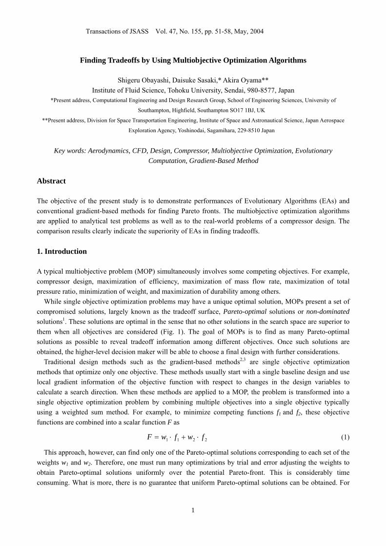
Transactions of JSASS Vol. 47, No. 155, pp. 51-58, May, 2004

1

Finding Tradeoffs by Using Multiobjective Optimization Algorithms

Shigeru Obayashi, Daisuke Sasaki,* Akira Oyama** Institute of Fluid Science, Tohoku University, Sendai, 980-8577, Japan

*Present address, Computational Engineering and Design Research Group, School of Engineering Sciences, University of

Southampton, Highfield, Southampton SO17 1BJ, UK

**Present address, Division for Space Transportation Engineering, Institute of Space and Astronautical Science, Japan Aerospace

Exploration Agency, Yoshinodai, Sagamihara, 229-8510 Japan

Key words: Aerodynamics, CFD, Design, Compressor, Multiobjective Optimization, Evolutionary

Computation, Gradient-Based Method Abstract The objective of the present study is to demonstrate performances of Evolutionary Algorithms (EAs) and conventional gradient-based methods for finding Pareto fronts. The multiobjective optimization algorithms are applied to analytical test problems as well as to the real-world problems of a compressor design. The comparison results clearly indicate the superiority of EAs in finding tradeoffs. 1. Introduction A typical multiobjective problem (MOP) simultaneously involves some competing objectives. For example, compressor design, maximization of efficiency, maximization of mass flow rate, maximization of total pressure ratio, minimization of weight, and maximization of durability among others.

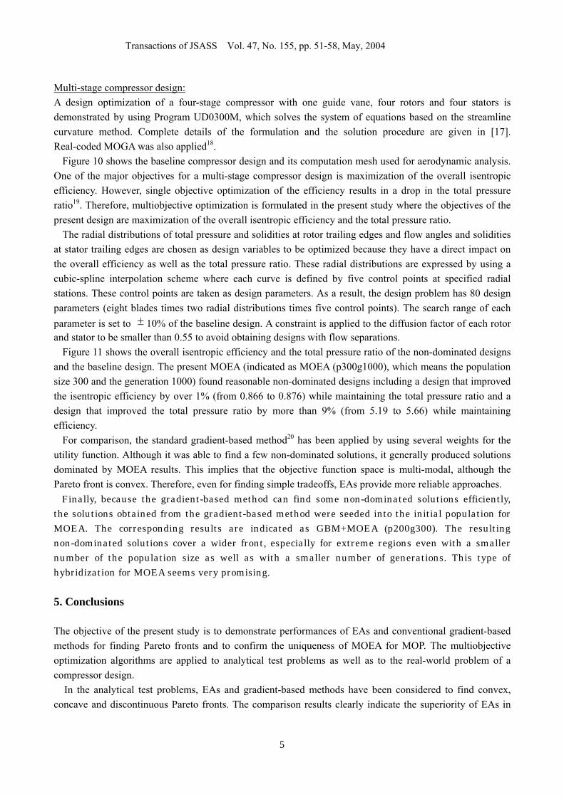
While single objective optimization problems may have a unique optimal solution, MOPs present a set of compromised solutions, largely known as the tradeoff surface, Pareto-optimal solutions or non-dominated solutions1. These solutions are optimal in the sense that no other solutions in the search space are superior to them when all objectives are considered (Fig. 1). The goal of MOPs is to find as many Pareto-optimal solutions as possible to reveal tradeoff information among different objectives. Once such solutions are obtained, the higher-level decision maker will be able to choose a final design with further considerations.

Traditional design methods such as the gradient-based methods2,3 are single objective optimization methods that optimize only one objective. These methods usually start with a single baseline design and use local gradient information of the objective function with respect to changes in the design variables to calculate a search direction. When these methods are applied to a MOP, the problem is transformed into a single objective optimization problem by combining multiple objectives into a single objective typically using a weighted sum method. For example, to minimize competing functions f1 and f2, these objective functions are combined into a scalar function F as

2211 fwfwF ⋅+⋅= (1)

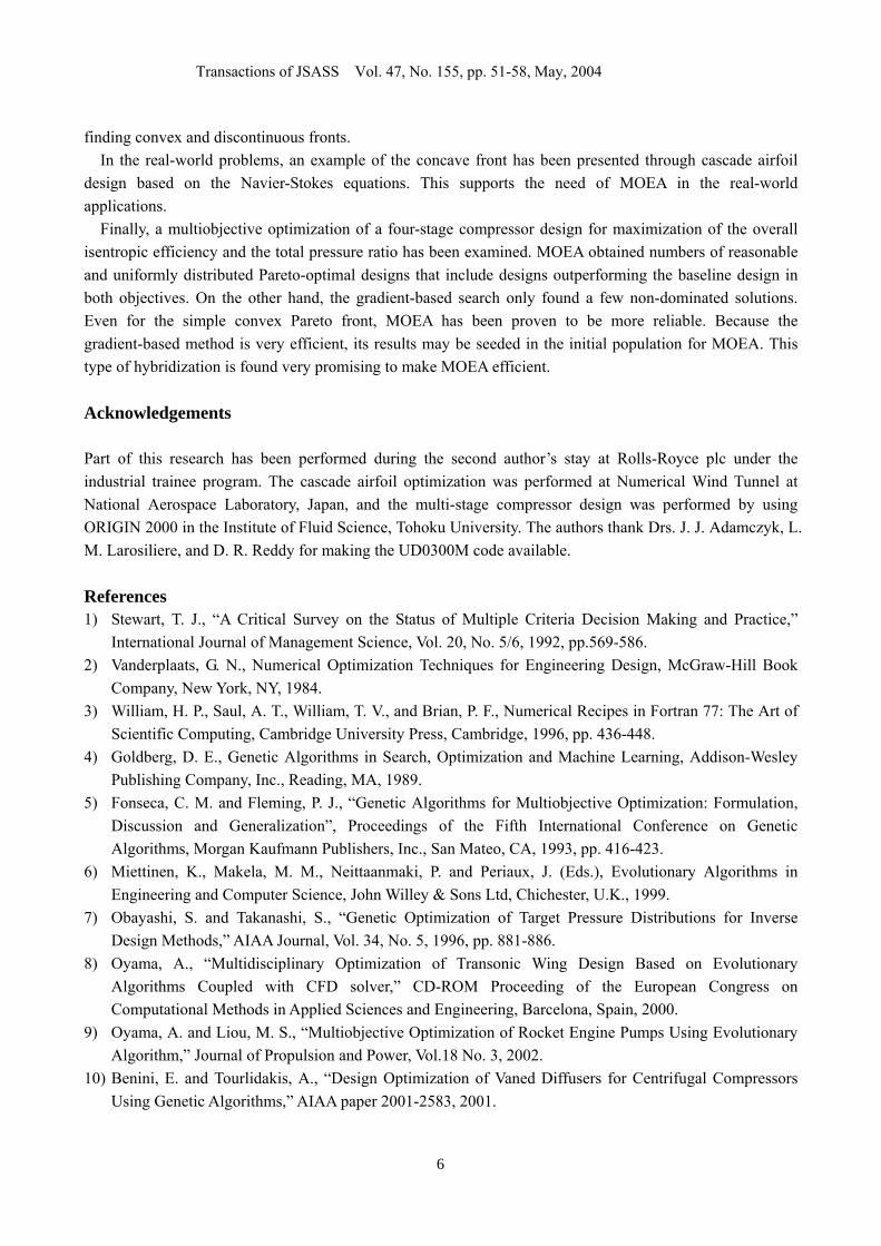
This approach, however, can find only one of the Pareto-optimal solutions corresponding to each set of the weights w1 and w2. Therefore, one must run many optimizations by trial and error adjusting the weights to obtain Pareto-optimal solutions uniformly over the potential Pareto-front. This is considerably time consuming. What is more, there is no guarantee that uniform Pareto-optimal solutions can be obtained. For


2

example, when this approach is applied to a MOP that has a concave tradeoff surface, it converges to two extreme optimums without showing any tradeoff information between the objectives (Fig. 2).

Evolutionary Algorithms (EAs, for example, see [4,5]), on the other hand, are particularly suited for MOPs. By maintaining a population of design candidates and using a fitness assignment method based on the Pareto-optimality concept, they can uniformly sample various Pareto-optimal solutions in one optimization without converting a MOP into a single objective problem. In addition, EAs have other advantages such as robustness, efficiency, as well as suitability for parallel computing. Due to these advantages, EAs are a unique and attractive approach to real-world design optimization problems such as the multi-stage compressor design optimization problem. Recently, EAs have been successfully applied to single objective and multiobjective aerospace design optimization problems6-10.

The objective of the present study is to make comparisons of EAs and conventional gradient-based methods to find Pareto fronts and to confirm the uniqueness of the multiobjective evolutionary algorithm (MOEA). The Multiobjective optimization algorithms are applied to analytical test problems as well as to the real-world problem of a compressor design.

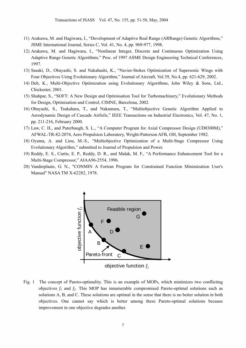
2. ARMOGA To reduce the large computational burden, the reduction of the total number of evaluations is needed. On the other hand, a large string length is necessary for real parameter problems. ARGA, which originally was proposed by Arakawa and Hagiwara, is a unique approach to solve such problems efficiently11,12. Real-coded ARGA has been developed and applied to aerodynamic optimization problems8,13.

ARMOGA has been developed based on ARGA to deal with multiple Pareto solutions for multi-objective optimization. The main difference between ARMOGA and conventional Multi-Objective Genetic Algorithm (MOGA) is the introduction of the range adaptation. The flowchart of present ARMOGA is shown in Fig. 3. Population is reinitialized every M generations for the range adaptation so that the population advances toward promising regions.

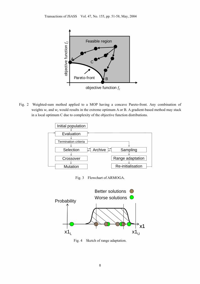
The basis of ARMOGA is the same as ARGA, but a straightforward extension may cause a problem in the diversity of the population. To better preserve the diversity of solution candidates, the normal distribution for encoding is changed. Figure 4 shows the search range with the distribution of the probability. Plateau regions are defined by the design ranges of chosen solutions. Then the normal distribution is considered the side of the plateau.

The advantages of ARMOGA are the following: It is possible to obtain Pareto solutions efficiently because of the concentrated search of the probable design space. In addition, it prevents the convergence to similar solutions. On the other hand, it may be difficult to avoid the local minima, if global solutions are not included in the present search region. Re-initialization also causes the time penalty. 3. Analytical Test Problems In this section, ARMOGA is evaluated by applying it to three different types of MO analytical problems. ARMOGA is compared with another MOEA and two gradient-based methods: NSGA214 (a widely-used MOEA), SQP (efficient gradient-based method) and DHC (robust gradient-based method). SQP and DHC in SOFT15 (Smart Optimization For Turbomachinery), developed by Rolls-Royce plc and University Technology Center, are used. Those gradient-based methods require the following utility function to solve


3

MO problems.

21 ffF ⋅+⋅= βα (2)

The search performance of ARMOGA is evaluated in terms of improvement in Pareto front, reasonable spread in Pareto front and more solutions in Pareto front as shown in Fig. 5. Those characteristics will help to understand the trade-off between objectives easily. For the purpose of aerodynamic optimization, ARMOGA and NSGA2 use a comparatively small number of evaluations.

Convex Pareto front case: This problem has two objective functions to be minimized as formulated below.

Min. ( ) ∑ ==

n

i ixn

f1

21

1x ,

Min. ( ) ( )∑ =−=

n

i ixn

f1

22 21x ,

subject to 44 ≤≤− ix , i = 1,2. (3)

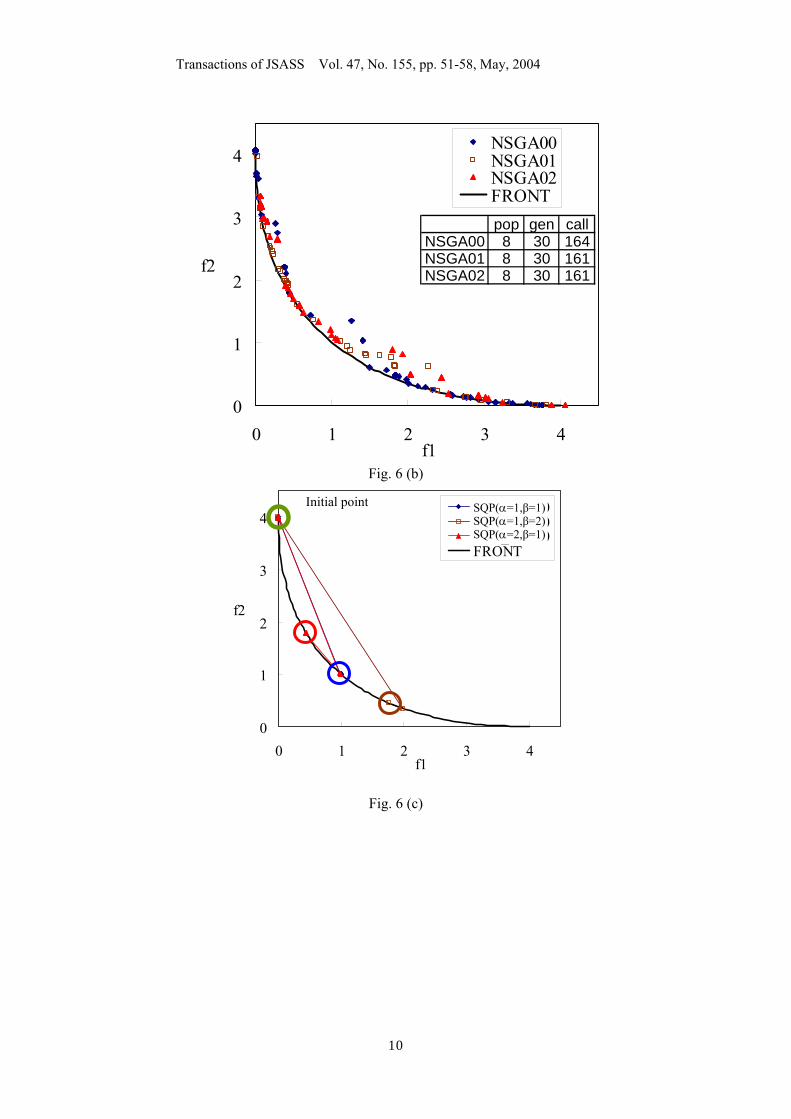
Pareto-optimal solutions have xi in [0,2] and the corresponding Pareto front is convex. Therefore, it is easy to obtain Global Pareto solutions for gradient-based methods. Figures 6 (a) and (b) show the performance of ARMOGA and NSGA2. As GA often depends on initial population, three different initial populations are used by giving different seeds for the random number generator for the comparison. From the figures, those two algorithms show the similar search performance. Figures 6 (c) and (d) show the search history of SQP and DHC. Those two algorithms obtain same final Pareto solutions by changing the weights of utility function described in Table 1. The only the difference is the number of evaluations. SQP could obtain final Pareto solutions rapidly. On the other hand, DHC requires a large number of evaluations similar to MOEAs.

Concave Pareto front case: This problem has a concave Pareto front. The problem is formulated as follows.

Min. ( ) ⎟⎟⎠

⎞⎜⎜⎝

⎛⎟⎠⎞

⎜⎝⎛ −−−= ∑ =

2

111exp1 n

i i nxf x ,

Min. ( ) ⎟⎟⎠

⎞⎜⎜⎝

⎛⎟⎠⎞

⎜⎝⎛ +−−= ∑ =

2

121exp1 n

i i nxf x ,

subject to 44 ≤≤− ix , i = 1,2. (4)

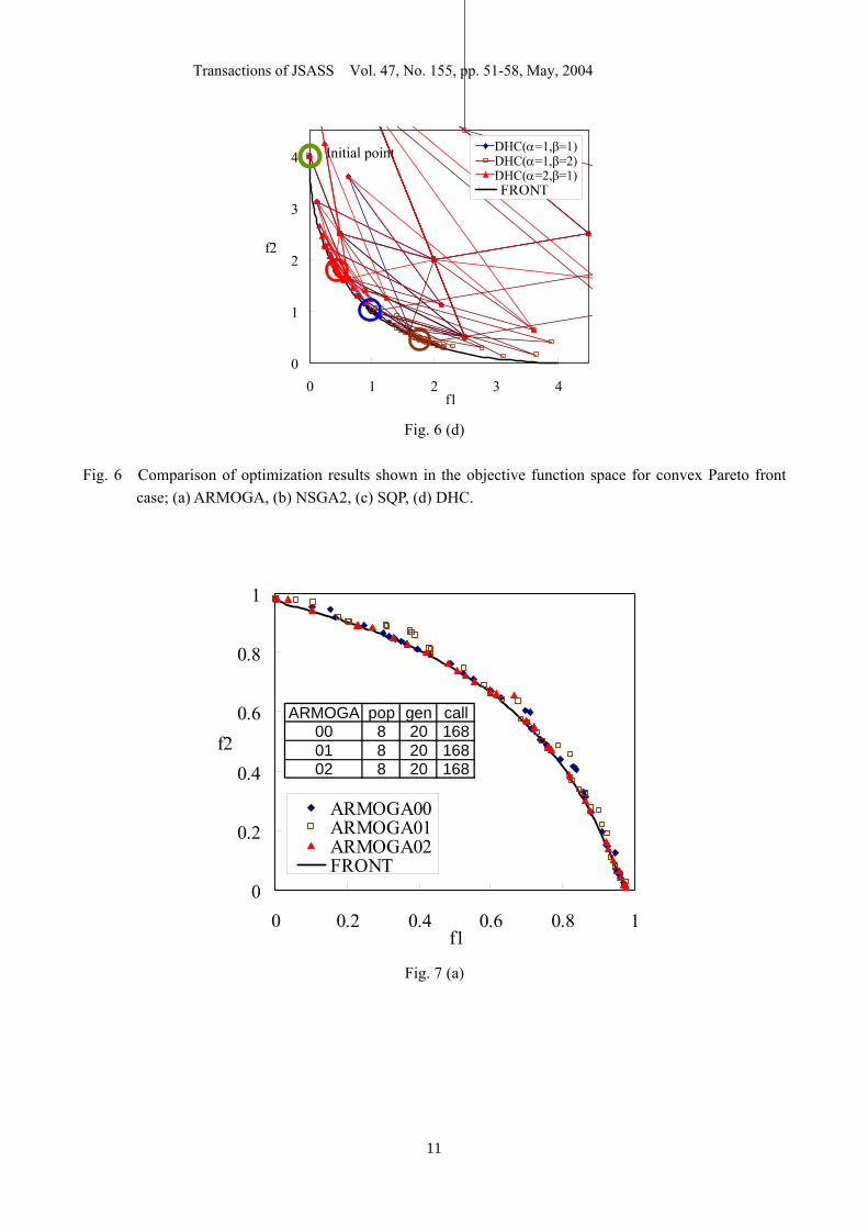
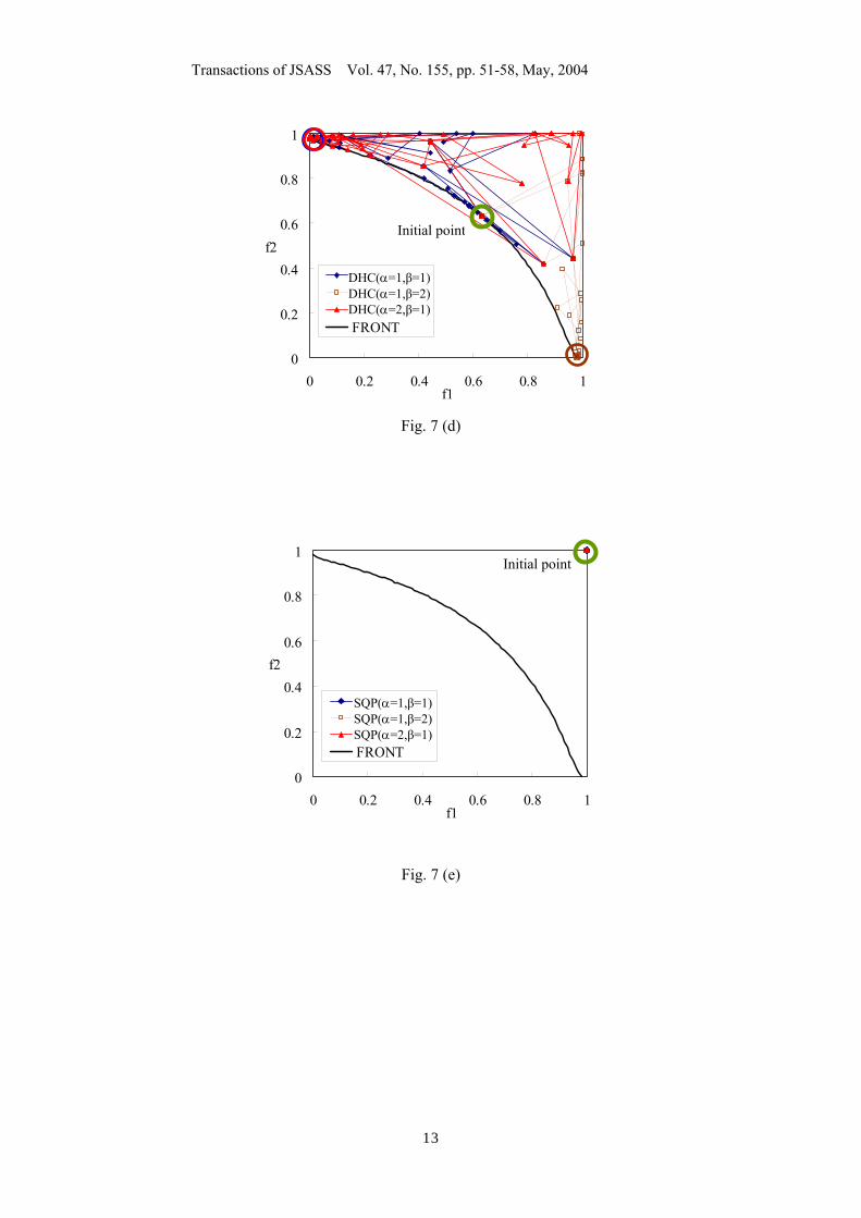
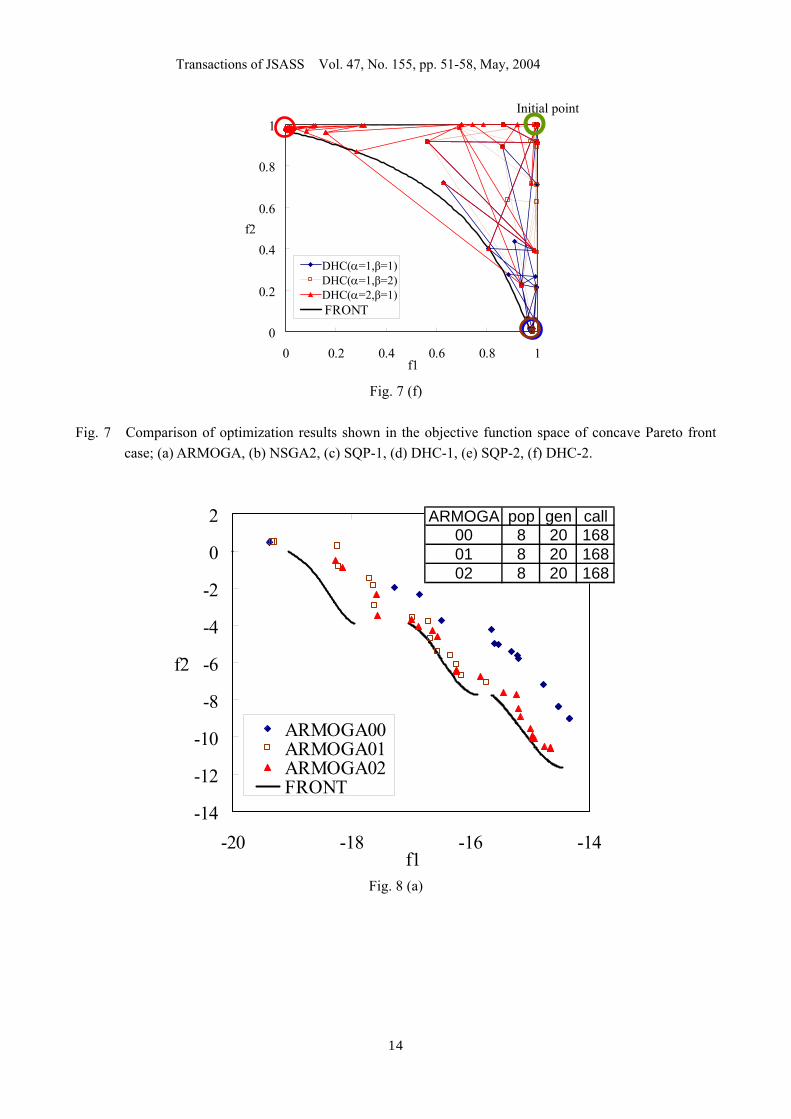
Figures 7 (a) and (b) show the non-dominated front of ARMOGA and NSGA2. Both GAs can obtain approximate Pareto solutions with a reasonable spread. On the other hand, it is difficult to obtain Pareto solutions by the gradient-based methods using a weight function because a final solution always becomes the extreme Pareto solution as shown in Figures 7 (c) – (f). Initial points for SQP-1 and SQP-2 are different. SQP-2 cannot obtain Pareto solutions. DHC-2 starts from the same point as SQP-2, but it is able to find the global Pareto solutions because DHC is more robust. Table 2 shows the summary of this optimization based on the gradient-based methods.


4

Discontinuous Pareto front: This problem has a nonconvex as well as disconnected Pareto-optimal set. It has three disconnected Pareto-optimal fronts and single point (-20,0).

Min. ( ) ( )[ ]∑ = ++−−=2

12

12

1 2.0exp10i ii xxf x ,

Min. ( ) ( )∑ =+=

3

138.0

2 sin5i ii xxf x ,

subject to 55 ≤≤− ix , i = 1,2,3. (5)

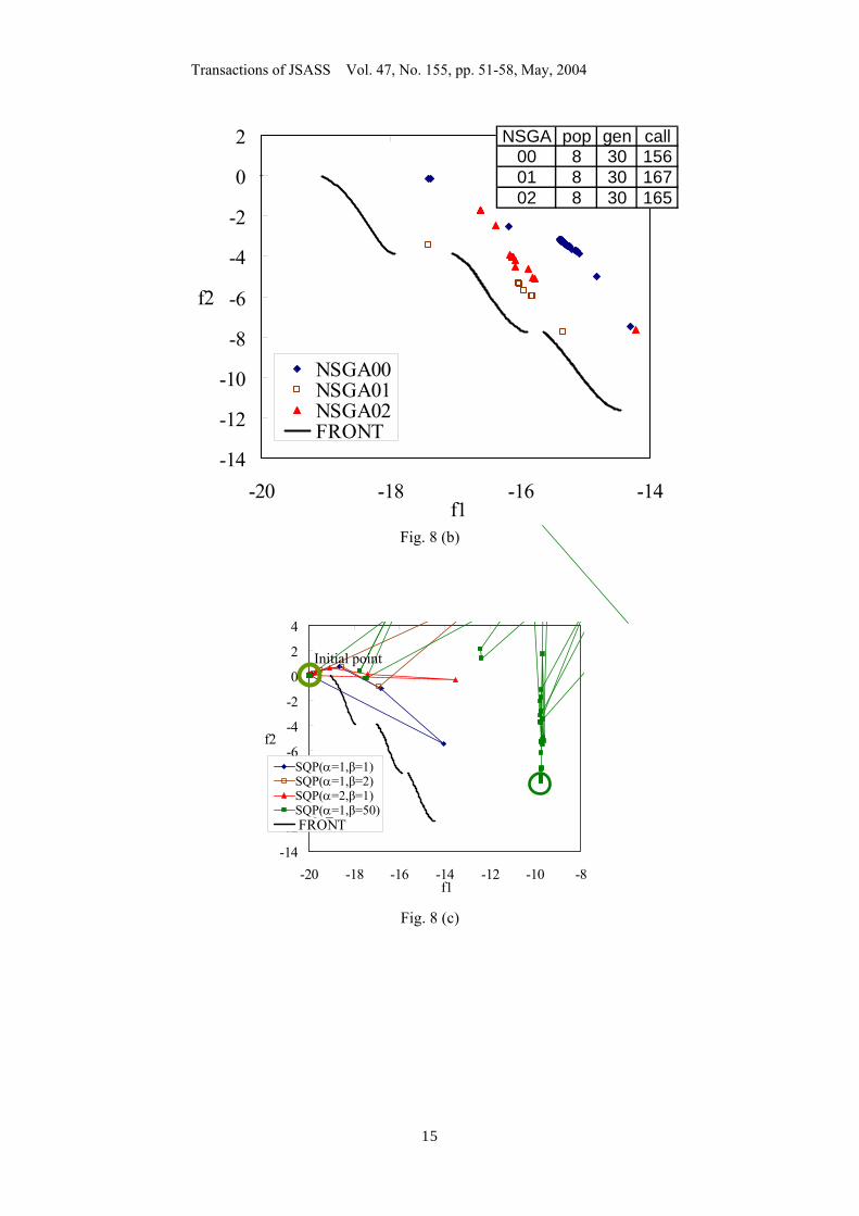
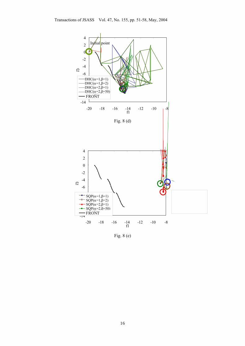
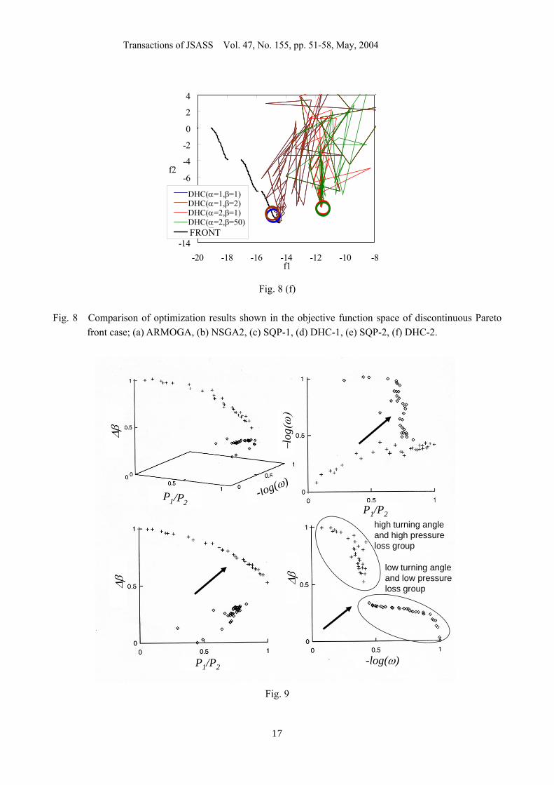
ARMOGA can obtain a good spread in Pareto front compared to NSGA2 as shown in Fig. 8. Figures 8 (c) – (f) show the search history of gradient-based methods and also Table 3 summarizes the optimization results.

Those three MO test cases show the following: 1) MOEAs can find trade-offs effectively. 2) ARMOGA is slightly superior to NSGA2 in the present cases. 3) Their computational costs are comparable to DHC. On the other hand, the gradient-based methods are not suitable for the aim of obtaining trade-offs, although DHC is slightly more robust than SQP. GAs may be more useful for multi-objective, multi-disciplinary aerodynamic optimization. 4. Real-world examples Aerodynamic design for cascade airfoils: Real-world engineering problems often exhibit straightforward convex tradeoffs. This leads to a question whether multiobjective optimization really needs to address concave and discontinuous Pareto fronts. This question is easily answered by a counterexample below.

The goal of the compressor design is to produce the highest pressure rise at the lowest total pressure loss. In addition to these two design goals, the flow turning angle is maximized in Ref. 16. The flow turning angle is an important design criterion in the classical design procedure. In general, the pressure rise increases as the flow turning angle increases. However, there is a limit in the amount of flow turning due to flow separation, causing large total pressure loss.

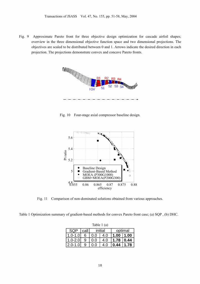
The present multiobjective optimization was performed to seek cascade airfoil shapes that 1. Maximize pressure rise as ratio of outlet to inlet pressures, P2/P1

2. Maximize flow turning angle, β∆

3. Minimize total pressure loss, ω subject to geometric constraints in the airfoil thickness and area. The two-dimensional Navier-Stokes code was used for the flow evaluation. Evolution was simulated for 75 generations with the population size of 64. Real-coded MOGA was applied because ARMOGA was not available yet.

The resulting approximate Pareto front is plotted in Fig. 9. Tradeoffs projected onto three combinations of the two objectives show convex and concave Pareto fronts. Those figures show the danger in the use of utility functions because it is possible to misunderstand the trade-off between objectives based on the gradient-based methods.


5

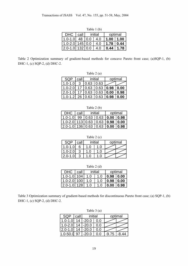
Multi-stage compressor design: A design optimization of a four-stage compressor with one guide vane, four rotors and four stators is demonstrated by using Program UD0300M, which solves the system of equations based on the streamline curvature method. Complete details of the formulation and the solution procedure are given in [17]. Real-coded MOGA was also applied18.

Figure 10 shows the baseline compressor design and its computation mesh used for aerodynamic analysis. One of the major objectives for a multi-stage compressor design is maximization of the overall isentropic efficiency. However, single objective optimization of the efficiency results in a drop in the total pressure ratio19. Therefore, multiobjective optimization is formulated in the present study where the objectives of the present design are maximization of the overall isentropic efficiency and the total pressure ratio.

The radial distributions of total pressure and solidities at rotor trailing edges and flow angles and solidities at stator trailing edges are chosen as design variables to be optimized because they have a direct impact on the overall efficiency as well as the total pressure ratio. These radial distributions are expressed by using a cubic-spline interpolation scheme where each curve is defined by five control points at specified radial stations. These control points are taken as design parameters. As a result, the design problem has 80 design parameters (eight blades times two radial distributions times five control points). The search range of each parameter is set to ± 10% of the baseline design. A constraint is applied to the diffusion factor of each rotor and stator to be smaller than 0.55 to avoid obtaining designs with flow separations.

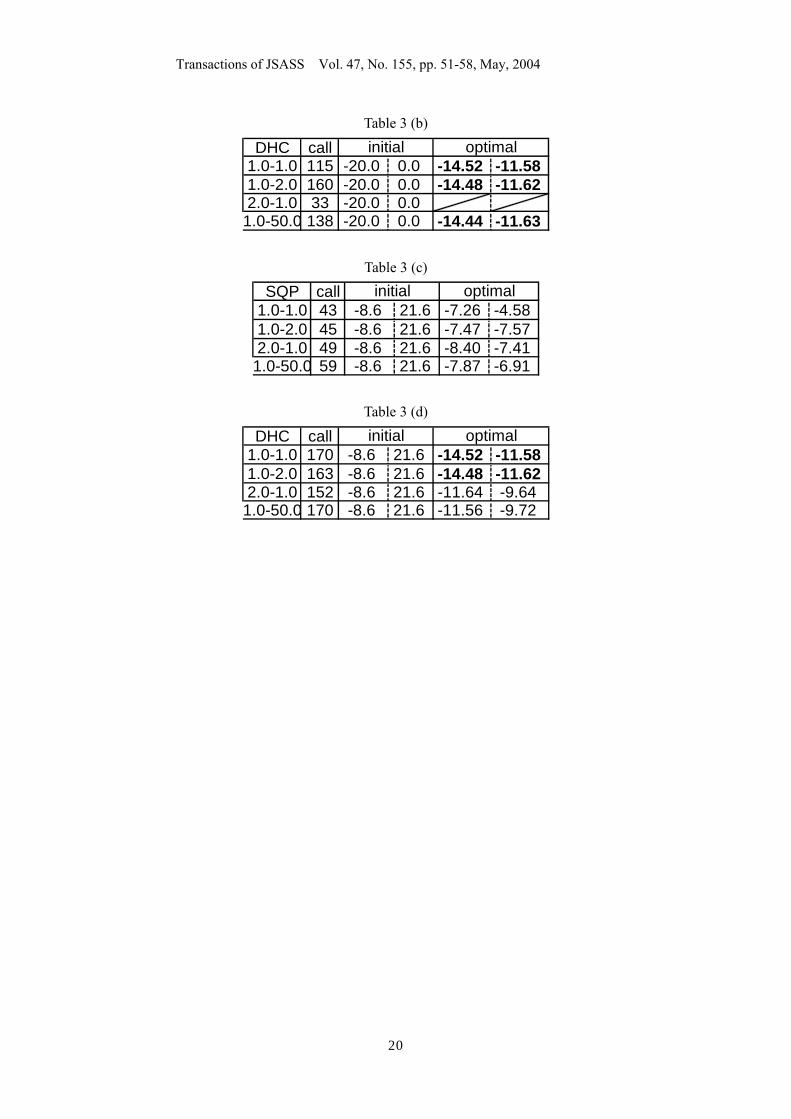
Figure 11 shows the overall isentropic efficiency and the total pressure ratio of the non-dominated designs and the baseline design. The present MOEA (indicated as MOEA (p300g1000), which means the population size 300 and the generation 1000) found reasonable non-dominated designs including a design that improved the isentropic efficiency by over 1% (from 0.866 to 0.876) while maintaining the total pressure ratio and a design that improved the total pressure ratio by more than 9% (from 5.19 to 5.66) while maintaining efficiency.

For comparison, the standard gradient-based method20 has been applied by using several weights for the utility function. Although it was able to find a few non-dominated solutions, it generally produced solutions dominated by MOEA results. This implies that the objective function space is multi-modal, although the Pareto front is convex. Therefore, even for finding simple tradeoffs, EAs provide more reliable approaches.

Finally, because the gradient-based method can find some non-dominated solutions efficiently, the solutions obtained from the gradient-based method were seeded into the initial population for MOEA. The corresponding results are indicated as GBM+MOEA (p200g300). The resulting non-dominated solutions cover a wider front, especially for extreme regions even with a smaller number of the population size as well as with a smaller number of generations. This type of hybridization for MOEA seems very promising.

5. Conclusions The objective of the present study is to demonstrate performances of EAs and conventional gradient-based methods for finding Pareto fronts and to confirm the uniqueness of MOEA for MOP. The multiobjective optimization algorithms are applied to analytical test problems as well as to the real-world problem of a compressor design.

In the analytical test problems, EAs and gradient-based methods have been considered to find convex, concave and discontinuous Pareto fronts. The comparison results clearly indicate the superiority of EAs in


6

finding convex and discontinuous fronts. In the real-world problems, an example of the concave front has been presented through cascade airfoil

design based on the Navier-Stokes equations. This supports the need of MOEA in the real-world applications.

Finally, a multiobjective optimization of a four-stage compressor design for maximization of the overall isentropic efficiency and the total pressure ratio has been examined. MOEA obtained numbers of reasonable and uniformly distributed Pareto-optimal designs that include designs outperforming the baseline design in both objectives. On the other hand, the gradient-based search only found a few non-dominated solutions. Even for the simple convex Pareto front, MOEA has been proven to be more reliable. Because the gradient-based method is very efficient, its results may be seeded in the initial population for MOEA. This type of hybridization is found very promising to make MOEA efficient.

Acknowledgements Part of this research has been performed during the second author’s stay at Rolls-Royce plc under the industrial trainee program. The cascade airfoil optimization was performed at Numerical Wind Tunnel at National Aerospace Laboratory, Japan, and the multi-stage compressor design was performed by using ORIGIN 2000 in the Institute of Fluid Science, Tohoku University. The authors thank Drs. J. J. Adamczyk, L. M. Larosiliere, and D. R. Reddy for making the UD0300M code available. References 1) Stewart, T. J., “A Critical Survey on the Status of Multiple Criteria Decision Making and Practice,”

International Journal of Management Science, Vol. 20, No. 5/6, 1992, pp.569-586. 2) Vanderplaats, G. N., Numerical Optimization Techniques for Engineering Design, McGraw-Hill Book

Company, New York, NY, 1984. 3) William, H. P., Saul, A. T., William, T. V., and Brian, P. F., Numerical Recipes in Fortran 77: The Art of

Scientific Computing, Cambridge University Press, Cambridge, 1996, pp. 436-448. 4) Goldberg, D. E., Genetic Algorithms in Search, Optimization and Machine Learning, Addison-Wesley

Publishing Company, Inc., Reading, MA, 1989. 5) Fonseca, C. M. and Fleming, P. J., “Genetic Algorithms for Multiobjective Optimization: Formulation,

Discussion and Generalization”, Proceedings of the Fifth International Conference on Genetic Algorithms, Morgan Kaufmann Publishers, Inc., San Mateo, CA, 1993, pp. 416-423.

6) Miettinen, K., Makela, M. M., Neittaanmaki, P. and Periaux, J. (Eds.), Evolutionary Algorithms in Engineering and Computer Science, John Willey & Sons Ltd, Chichester, U.K., 1999.

7) Obayashi, S. and Takanashi, S., “Genetic Optimization of Target Pressure Distributions for Inverse Design Methods,” AIAA Journal, Vol. 34, No. 5, 1996, pp. 881-886.

8) Oyama, A., “Multidisciplinary Optimization of Transonic Wing Design Based on Evolutionary Algorithms Coupled with CFD solver,” CD-ROM Proceeding of the European Congress on Computational Methods in Applied Sciences and Engineering, Barcelona, Spain, 2000.

9) Oyama, A. and Liou, M. S., “Multiobjective Optimization of Rocket Engine Pumps Using Evolutionary Algorithm,” Journal of Propulsion and Power, Vol.18 No. 3, 2002.

10) Benini, E. and Tourlidakis, A., “Design Optimization of Vaned Diffusers for Centrifugal Compressors Using Genetic Algorithms,” AIAA paper 2001-2583, 2001.


7

11) Arakawa, M. and Hagiwara, I., “Development of Adaptive Real Range (ARRange) Genetic Algorithms,” JSME International Journal, Series C, Vol. 41, No. 4, pp. 969-977, 1998.

12) Arakawa, M. and Hagiwara, I., “Nonlinear Integer, Discrete and Continuous Optimization Using Adaptive Range Genetic Algorithms,” Proc. of 1997 ASME Design Engineering Technical Conferences, 1997.

13) Sasaki, D., Obayashi, S. and Nakahashi, K., “Navier-Stokes Optimization of Supersonic Wings with Four Objectives Using Evolutionary Algorithm,” Journal of Aircraft, Vol.39, No.4, pp. 621-629, 2002.

14) Deb, K., Multi-Objective Optimization using Evolutionary Algorithms, John Wiley & Sons, Ltd., Chickester, 2001.

15) Shahpar, S., “SOFT: A New Design and Optimisation Tool for Turbomachinery,” Evolutionary Methods for Design, Optimisation and Control, CIMNE, Barcelona, 2002.

16) Obayashi, S., Tsukahara, T., and Nakamura, T., “Multiobjective Genetic Algorithm Applied to Aerodynamic Design of Cascade Airfoils,” IEEE Transactions on Industrial Electronics, Vol. 47, No. 1, pp. 211-216, February 2000.

17) Law, C. H., and Puterbaugh, S. L., “A Computer Program for Axial Compressor Design (UD0300M),” AFWAL-TR-82-2074, Aero Propulsion Laboratory, Wright-Patterson AFB, OH, September 1982.

18) Oyama, A. and Liou, M.-S., “Multiobjective Optimization of a Mulit-Stage Compressor Using Evolutionary Algorithm,” submitted to Journal of Propulsion and Power.

19) Reddy, E. S., Curtis, E. P., Reddy, D. R., and Malak, M. F., “A Performance Enhancement Tool for a Multi-Stage Compressor,” AIAA96-2554, 1996.

20) Vanderplaats, G. N., "CONMIN A Fortran Program for Constrained Function Minimization User's Manual" NASA TM X-62282, 1978.

Pareto-front

A

B

obje

ctiv

e fu

nctio

n f 2

objective function f1

C

Feasible region

D

E

FG

Fig. 1 The concept of Pareto-optimality. This is an example of MOPs, which minimizes two conflicting objectives f1 and f2. This MOP has innumerable compromised Pareto-optimal solutions such as solutions A, B, and C. These solutions are optimal in the sense that there is no better solution in both objectives. One cannot say which is better among these Pareto-optimal solutions because improvement in one objective degrades another.


8

Pareto-front

Feasible region

A

B

obje

ctiv

e fu

nctio

n f 2


C

Fig. 2 Weighted-sum method applied to a MOP having a concave Pareto-front. Any combination of weights w1 and w2 would results in the extreme optimum A or B. A gradient-based method may stack in a local optimum C due to complexity of the objective function distributions.

Initial population

Evaluation

Selection

Crossover

Mutation

Termination criteria

Sampling

Range adaptation

Re-initialisation

Archive

Fig. 3 Flowchart of ARMOGA.

x1x1x1L x1U

Better solutionsWorse solutions

Probability

Fig. 4 Sketch of range adaptation.


9

Pareto-front

A(1)

B(1)

obje

ctiv

e fu

nctio

n f 2


C(1)

Feasible region

D(2)

E(2)

F(3) G(6)

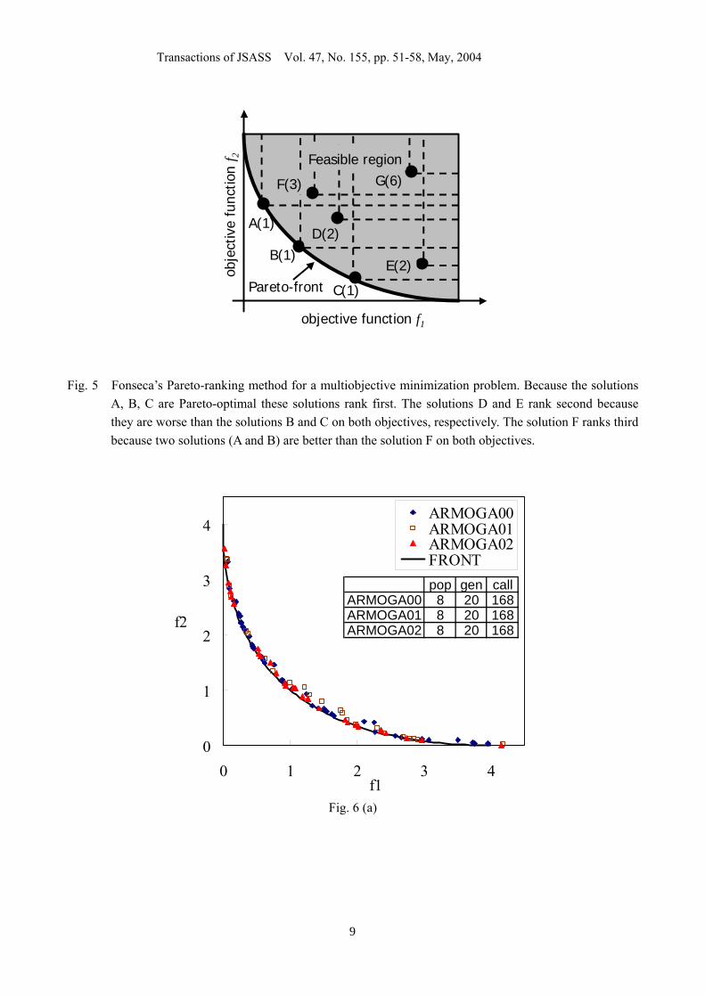
Fig. 5 Fonseca’s Pareto-ranking method for a multiobjective minimization problem. Because the solutions A, B, C are Pareto-optimal these solutions rank first. The solutions D and E rank second because they are worse than the solutions B and C on both objectives, respectively. The solution F ranks third because two solutions (A and B) are better than the solution F on both objectives.

0

1

2

3

4

0 1 2 3 4f1

f2

ARMOGA00ARMOGA01ARMOGA02FRONTpop gen call

ARMOGA00 8 20 168ARMOGA01 8 20 168ARMOGA02 8 20 168

Fig. 6 (a)


10

0

1

2

3

4

0 1 2 3 4f1

f2

NSGA00NSGA01NSGA02FRONTpop gen call

NSGA00 8 30 164NSGA01 8 30 161NSGA02 8 30 161

Fig. 6 (b)

0

1

2

3

4

0 1 2 3 4f1

f2

SQP_1.0-1.0SQP_1.0-2.0SQP_2.0-1.0FRONT

Fig. 6 (c)

SQP(α=1,β=1)SQP(α=1,β=2)SQP(α=2,β=1)

Initial point


11

0

1

2

3

4

0 1 2 3 4f1

f2

DHC_1.0-1.0DHC_1.0-2.0DHC_2.0-1.0FRONT

Fig. 6 (d)

Fig. 6 Comparison of optimization results shown in the objective function space for convex Pareto front

case; (a) ARMOGA, (b) NSGA2, (c) SQP, (d) DHC.

0

0.2

0.4

0.6

0.8

1

0 0.2 0.4 0.6 0.8 1f1

f2

ARMOGA00ARMOGA01ARMOGA02FRONT

ARMOGA pop gen call00 8 20 16801 8 20 16802 8 20 168

Fig. 7 (a)

DHC(α=1,β=1)DHC(α=1,β=2)DHC(α=2,β=1)

Initial point


12

0

0.2

0.4

0.6

0.8

1

0 0.2 0.4 0.6 0.8 1f1

f2

NSGA00NSGA01NSGA02FRONT

NSGA pop gen call00 8 30 15901 8 30 10802 8 30 171

Fig. 7 (b)

0

0.2

0.4

0.6

0.8

1

0 0.2 0.4 0.6 0.8 1f1

f2

SQP_1.0-1.0SQP_1.0-2.0SQP_2.0-1.0SQP_1.0-1.2FRONT

Fig. 7 (c)

SQP(α=1,β=1)SQP(α=1,β=2)SQP(α=2,β=1)SQP(α=2,β=1.2)

Initial point


13

0

0.2

0.4

0.6

0.8

1

0 0.2 0.4 0.6 0.8 1f1

f2

DHC_1.0-1.0DHC_1.0-2.0DHC_2.0-1.0FRONT

Fig. 7 (d)

0

0.2

0.4

0.6

0.8

1

0 0.2 0.4 0.6 0.8 1f1

f2

SQP_1.0-1.0SQP_1.0-2.0SQP_2.0-1.0FRONT

Fig. 7 (e)


Initial point

SQP(α=1,β=1)SQP(α=1,β=2)SQP(α=2,β=1)

Initial point


14

0

0.2

0.4

0.6

0.8

1

0 0.2 0.4 0.6 0.8 1f1

f2

DHC_1.0-1.0DHC_1.0-2.0DHC_2.0-1.0FRONT

Fig. 7 (f)

Fig. 7 Comparison of optimization results shown in the objective function space of concave Pareto front

case; (a) ARMOGA, (b) NSGA2, (c) SQP-1, (d) DHC-1, (e) SQP-2, (f) DHC-2.

-14

-12

-10

-8

-6

-4

-2

0

2

-20 -18 -16 -14f1

f2

ARMOGA00ARMOGA01ARMOGA02FRONT

ARMOGA pop gen call00 8 20 16801 8 20 16802 8 20 168

Fig. 8 (a)


Initial point


15

-14

-12

-10

-8

-6

-4

-2

0

2

-20 -18 -16 -14f1

f2

NSGA00NSGA01NSGA02FRONT

NSGA pop gen call00 8 30 15601 8 30 16702 8 30 165

Fig. 8 (b)

-14

-12

-10

-8

-6

-4

-2

0

2

4

-20 -18 -16 -14 -12 -10 -8f1

f2


Fig. 8 (c)

SQP(α=1,β=1)SQP(α=1,β=2)SQP(α=2,β=1)SQP(α=1,β=50)

Initial point


16

-14

-12

-10

-8

-6

-4

-2

0

2

4

-20 -18 -16 -14 -12 -10 -8f1

f2

DHC_1.0-1.0DHC_1.0-2.0DHC_2.0-1.0DHC_1.0-50.0FRONT

Fig. 8 (d)

-14

-12

-10

-8

-6

-4

-2

0

2

4

-20 -18 -16 -14 -12 -10 -8f1

f2


Fig. 8 (e)

DHC(α=1,β=1)DHC(α=1,β=2)DHC(α=2,β=1)DHC(α=2,β=50)

Initial point

SQP(α=1,β=1)SQP(α=1,β=2)SQP(α=2,β=1)SQP(α=2,β=50)


17

-14

-12

-10

-8

-6

-4

-2

0

2

4

-20 -18 -16 -14 -12 -10 -8f1

f2

DHC_1.0-1.0DHC_1.0-2.0DHC_2.0-1.0DHC_1.0-50.0FRONT

Fig. 8 (f)

Fig. 8 Comparison of optimization results shown in the objective function space of discontinuous Pareto

front case; (a) ARMOGA, (b) NSGA2, (c) SQP-1, (d) DHC-1, (e) SQP-2, (f) DHC-2.

low turning angleand low pressure loss group

∆β∆β ∆β

−log(ω)

P1/P2

high turning angle and high pressure loss group

-log(ω)

P1/P2-log(ω)

P1/P2

Fig. 9

DHC(α=1,β=1)DHC(α=1,β=2)DHC(α=2,β=1)DHC(α=2,β=50)


18

Fig. 9 Approximate Pareto front for three objective design optimization for cascade airfoil shapes;

overview in the three dimensional objective function space and two dimensional projections. The objectives are scaled to be distributed between 0 and 1. Arrows indicate the desired direction in each projection. The projections demonstrate convex and concave Pareto fronts.

IGVS2S1 S4S3

R1 R4R3R2

Fig. 10 Four-stage axial compressor baseline design.

0.855 0.86 0.865 0.87 0.875 0.884.8

5

5.2

5.4

5.6

Baseline DesignGradient-Based MethodMOEA (P300G1000)GBM+MOEA(P200G300)

efficiency

Pt ra

tio

Fig. 11 Comparison of non-dominated solutions obtained from various approaches.

Table 1 Optimization summary of gradient-based methods for convex Pareto front case; (a) SQP , (b) DHC.

Table 1 (a)

SQP call1.0-1.0 6 0.0 4.0 1.00 1.001.0-2.0 9 0.0 4.0 1.78 0.442.0-1.0 9 0.0 4.0 0.44 1.78

initial optimal


19

Table 1 (b) DHC call

1.0-1.0 48 0.0 4.0 1.00 1.001.0-2.0 145 0.0 4.0 1.78 0.442.0-1.0 132 0.0 4.0 0.44 1.78

initial optimal

Table 2 Optimization summary of gradient-based methods for concave Pareto front case; (a)SQP-1, (b) DHC-1, (c) SQP-2, (d) DHC-2.

Table 2 (a)

SQP call1.0-1.0 3 0.63 0.631.0-2.0 17 0.63 0.63 0.98 0.002.0-1.0 17 0.63 0.63 0.00 0.981.0-1.2 26 0.63 0.63 0.98 0.00

initial optimal

Table 2 (b) DHC call

1.0-1.0 99 0.63 0.63 0.00 0.981.0-2.0 113 0.63 0.63 0.98 0.002.0-1.0 136 0.63 0.63 0.00 0.98

initial optimal

Table 2 (c) SQP call

1.0-1.0 6 1.0 1.01.0-2.0 3 1.0 1.02.0-1.0 3 1.0 1.0

initial optimal

Table 2 (d) DHC call

1.0-1.0 104 1.0 1.0 0.98 0.001.0-2.0 100 1.0 1.0 0.98 0.002.0-1.0 128 1.0 1.0 0.00 0.98

initial optimal

Table 3 Optimization summary of gradient-based methods for discontinuous Pareto front case; (a) SQP-1, (b) DHC-1, (c) SQP-2, (d) DHC-2.

Table 3 (a)

SQP call1.0-1.0 14 -20.0 0.01.0-2.0 14 -20.0 0.02.0-1.0 14 -20.0 0.0

1.0-50.0 97 -20.0 0.0 -9.75 -8.44

initial optimal


20

Table 3 (b)

DHC call1.0-1.0 115 -20.0 0.0 -14.52 -11.581.0-2.0 160 -20.0 0.0 -14.48 -11.622.0-1.0 33 -20.0 0.0

1.0-50.0 138 -20.0 0.0 -14.44 -11.63

initial optimal

Table 3 (c)

SQP call1.0-1.0 43 -8.6 21.6 -7.26 -4.581.0-2.0 45 -8.6 21.6 -7.47 -7.572.0-1.0 49 -8.6 21.6 -8.40 -7.41

1.0-50.0 59 -8.6 21.6 -7.87 -6.91

initial optimal

Table 3 (d)

DHC call1.0-1.0 170 -8.6 21.6 -14.52 -11.581.0-2.0 163 -8.6 21.6 -14.48 -11.622.0-1.0 152 -8.6 21.6 -11.64 -9.64

1.0-50.0 170 -8.6 21.6 -11.56 -9.72

initial optimal

finding tradeoffs by using multiobjective optimization ...finding tradeoffs by using multiobjective...

Documents