Finite Difference Schemes and the Schrodinger Equation

Jonathan King, Pawan Dhakal

June 2, 2014

1 Introduction

In this paper, we primarily explore numerical solutions to the Quantum 1D Infinite Square Well problem,and the 1D Quantum Scattering problem. We use different finite difference schemes to approximate thesecond derivative in the 1D Schrodinger’s Equation and linearize the problem. By doing so, we convert theInfinite Well problem to a simple Eigenvalue problem and the Scattering problem to a solution of a systemof linear equations. We examine the convergence of the solution to the infinite square well problem for highorder stencils, and compare the computed results to an analytic solution. For the scattering problem, we testboth first and second order finite difference schemes for boundary conditions, and compare the convergenceof these schemes.

2 Finite Difference Schemes

Finite Difference Methods are used to approximate derivates to solve differential equations numerically. Thegoal is to discretize the domain of the given problem, for example the x grid for a function f(x), and usethe value of the function evaluated at a point and neigbouring point(s) to approximate the derivative ofthe function at the point. The assumption made is that the functions to be differentiated are well behaved.Then using truncated taylor’s sum, one can derive approximations for derivatives. In our project, we neededapproximations for the first derivative and the second derivative.

2.1 Stencils and Differences

Depending on the number of neighbouring points used in approximate derivatives, we can define our approx-imation as being the ’three point stencil’ if we are using two neighbouring points along with the evaluationpoint, or as the ’five point stencil’ if we are using four neighbouring points along with the evaluation pointand so on.Similarly, we can define our approximations as being centered difference, backward difference, or forward

difference depending upon the symmetry of the neighbouring points. For example: u′ ≈ ui+1 − ui∆x

is

the forward (two point stencil) finite difference method for approximating first derivative of u. Similarly,

u′ ≈ ui+1 − ui−12∆x

is the centered finite difference method, and u′ ≈ ui − ui−1∆x

is the backward finite difference

method.

2.2 Deriving Coefficients and Accuracy

To derive the coefficients for finite difference, we use truncated taylor series to approximate the value ofthe function at the point of evaluation of the derivative and at the neighbouring points. We can use theleading term in truncated error (i.e. real sum - truncated sum) to approximate the error in the truncatedtaylor series and predict the accuracy of the approximate derivative. Using a general equivalence relationfn(x) ≈ ...+ af(x− h) + bf(x) + cf(x+ h) + ... depending upon the no of stencils and the type of difference(backward,forward, or centered) we want, we can find the coefficients a,b,c.. to approximate the nth deriva-tive of f.For the purposes of this project, we need the following approximations:

1

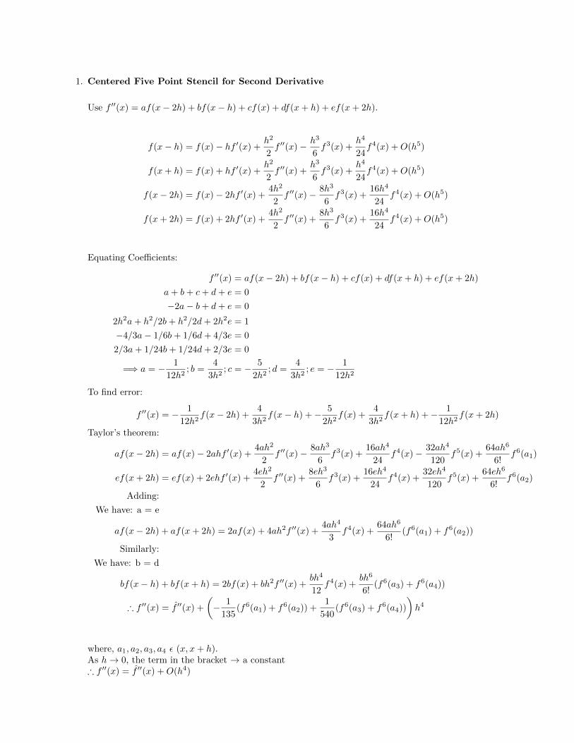
1. Centered Five Point Stencil for Second Derivative

Use f ′′(x) = af(x− 2h) + bf(x− h) + cf(x) + df(x+ h) + ef(x+ 2h).

f(x− h) = f(x)− hf ′(x) +h2

2f ′′(x)− h3

6f3(x) +

h4

24f4(x) +O(h5)

f(x+ h) = f(x) + hf ′(x) +h2

2f ′′(x) +

h3

6f3(x) +

h4

24f4(x) +O(h5)

f(x− 2h) = f(x)− 2hf ′(x) +4h2

2f ′′(x)− 8h3

6f3(x) +

16h4

24f4(x) +O(h5)

f(x+ 2h) = f(x) + 2hf ′(x) +4h2

2f ′′(x) +

8h3

6f3(x) +

16h4

24f4(x) +O(h5)

Equating Coefficients:

f ′′(x) = af(x− 2h) + bf(x− h) + cf(x) + df(x+ h) + ef(x+ 2h)

a+ b+ c+ d+ e = 0

−2a− b+ d+ e = 0

2h2a+ h2/2b+ h2/2d+ 2h2e = 1

−4/3a− 1/6b+ 1/6d+ 4/3e = 0

2/3a+ 1/24b+ 1/24d+ 2/3e = 0

=⇒ a = − 1

12h2; b =

4

3h2; c = − 5

2h2; d =

4

3h2; e = − 1

12h2

To find error:

f ′′(x) = − 1

12h2f(x− 2h) +

4

3h2f(x− h) +− 5

2h2f(x) +

4

3h2f(x+ h) +− 1

12h2f(x+ 2h)

Taylor’s theorem:

af(x− 2h) = af(x)− 2ahf ′(x) +4ah2

2f ′′(x)− 8ah3

6f3(x) +

16ah4

24f4(x)− 32ah4

120f5(x) +

64ah6

6!f6(a1)

ef(x+ 2h) = ef(x) + 2ehf ′(x) +4eh2

2f ′′(x) +

8eh3

6f3(x) +

16eh4

24f4(x) +

32eh4

120f5(x) +

64eh6

6!f6(a2)

Adding:

We have: a = e

af(x− 2h) + af(x+ 2h) = 2af(x) + 4ah2f ′′(x) +4ah4

3f4(x) +

64ah6

6!(f6(a1) + f6(a2))

Similarly:

We have: b = d

bf(x− h) + bf(x+ h) = 2bf(x) + bh2f ′′(x) +bh4

12f4(x) +

bh6

6!(f6(a3) + f6(a4))

∴ f ′′(x) = f ′′(x) +

(− 1

135(f6(a1) + f6(a2)) +

1

540(f6(a3) + f6(a4))

)h4

where, a1, a2, a3, a4 ε (x, x+ h).As h→ 0, the term in the bracket → a constant∴ f ′′(x) = f ′′(x) +O(h4)

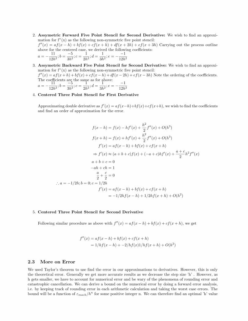
2. Assymetric Forward Five Point Stencil for Second Derivative: We wish to find an approxi-mation for f”(x) as the following non-symmetric five point stencil:f ′′(x) = af(x − h) + bf(x) + cf(x + h) + df(x + 2h) + ef(x + 3h) Carrying out the process outlineabove for the centered case, we derived the following coefficients:

a = − 11

12h2; b =

−5

3h2; c =

1

2h2; d =

1

3h2; e = − −1

12h2

3. Assymetric Backward Five Point Stencil for Second Derivative: We wish to find an approxi-mation for f”(x) as the following non-symmetric five point stencil:f ′′(x) = af(x+ h) + bf(x) + cf(x− h) + df(x− 2h) + ef(x− 3h) Note the ordering of the coefficients.The coefficients are the same as for above:

a = − 11

12h2; b =

−5

3h2; c =

1

2h2; d =

1

3h2; e = − −1

12h2

4. Centered Three Point Stencil for First Derivative

Approximating double derivative as f ′(x) = af(x−h)+bf(x)+cf(x+h), we wish to find the coefficientsand find an order of approximation for the error.

f(x− h) = f(x)− hf ′(x) +h2

2f ′′(x) +O(h3)

f(x+ h) = f(x) + hf ′(x) +h2

2f ′′(x) +O(h3)

f ′(x) = af(x− h) + bf(x) + cf(x+ h)

⇒ f ′(x) ≈ (a+ b+ c)f(x) + (−a+ c)hf ′(x) +a+ c

2h2f ′′(x)

a+ b+ c = 0

−ah+ ch = 1a

2+c

2= 0

∴ a = −1/2h; b = 0; c = 1/2h

f ′(x) = af(x− h) + bf(x) + cf(x+ h)

= −1/2hf(x− h) + 1/2hf(x+ h) +O(h2)

5. Centered Three Point Stencil for Second Derivative

Following similar procedure as above with f ′′(x) = af(x− h) + bf(x) + cf(x+ h), we get

f ′′(x) = af(x− h) + bf(x) + cf(x+ h)

= 1/hf(x− h) +−2/hf(x)1/hf(x+ h) +O(h2)

2.3 More on Error

We used Taylor’s theorem to use find the error in our approximations to derivatives. However, this is onlythe theoretical error. Generally we get more accurate results as we decrease the step size ’h’ . However, ash gets smaller, we have to account for numerical error and be wary of the phenomena of rounding error andcatastrophic cancellation. We can derive a bound on the numerical error by doing a forward error analysis,i.e. by keeping track of rounding error in each arithmetic calculation and taking the worst case errors. Thebound will be a function of εmach/h

n for some positive integer n. We can therefore find an optimal ’h’ value

for which our calculation will be the most accurate for a calculation of a derivative. We just need to equateour numerical error with our theoretical error due to taylor sum truncation, and solve for h.We could derive an optimal h step size for the case of a centered three point stencil approximation for thesecond derivative. But, note that our project involves eigenvalue calculation and linear system solving for1/h by 1/h size matrices (see below). To save computing time, we will not go beyond h = O(10−3) for ourstep sizes, and therefore error in our calculation will be dominated by the theoretical error due to truncationof taylor sum. The numerical error dominates only for very small h.

3 Solving the Schrodinger’s Equation

3.1 Eigenvalue Problem

The wavefunctions, u, are eigenvectors of the Hamiltonian operator, and satisfy the Schrodinger Equation:

H u = E u (1)

where H is the Hamiltonian Operator, and the eigenvalues E are the energies of a particle with wavefunctionu.

In the one dimensional case, u is dependent only on the spatial coordinate x, and the one dimensionalHamiltonian is given by

H =

(−~2m

)∂2

∂x2+ V (x)

where ~ is a constant, m is the mass of the particle, and V(x) defines the potential energy function for theparticle. Note that H is dependent upon x via the V(x) term. To give a dimensionless analysis, we define~ = 2m = 1, so that

H = − ∂2

∂x2+ V (x) (2)

Consider the points: xj j = 0, 1, 2...n.At each point xj , equation (1) holds, so that

Hj u(xj) = E u(xj)

where Hj is the Hamiltonian operator evaluated at V(xj . Considering each of the points xj gives thesystem of equations:

H0 u(x0) = E u(x0)H1 u(x1) = E u(x1)

...Hn u(xn) = E u(xn)

Using equation 2, this system can be written as:

−u′′(x0) + V (x0)u(x0) = Eu(x0)−u′′(x1) + V (x1)u(x1) = Eu(x1) (3)

...−u′′(xn) + V (xn)u(xn) = Eu(xn)

We now have a system of n equations relating the wavefunction of a particle to its energy. Given apotential function V(x), we wish to evaluate the wavefunction to high accuracy at each of the sample pointsu(xj). We will limit our analysis to potential functions that go to infinity at the boundaries a and b of ourgrid, and will assume that the points xj are equally spaced.

Note that this system consists of n solutions to the second order ODE

−u′′(x) + [V (x)− E]u(x) = 0

This will require two boundary conditions which will vary by the case being analyzed. We will limit ouranalysis the evaluation of u(xj) in the case of the infinite square well, and for scattering states within a finiteinterval.

We now choose to approximate u”(x) using a using some finite difference scheme for u”(x), such that:

u′′(xj) =

(1

h2

)(Au(xj−n) +Bu(xj−n+1) + ...+ Cu(xj) + ...+Du(xj+n−1) + Eu(xj+n))

where the coefficients A, B, C, D, and E are constants (that may be equal to zero), h is the step size,and n is an integer.

For the second order, centered finite difference approximation:

u′′(xj) ≈(

1

h2

)(u(xj−1)− 2u(xj) + u(xj+1))

system (3) becomes

−(

1

h2

)u(x−1) +

(V (x0) +

2

h2

)u(x0)− (

1

h2)u(x1) = Eu(x0)

−(

1

h2

)u(x0) +

(V (x1) +

2

h2

)u(x1)−

(1

h2

)u(x2) = Eu(x1)

...

−(

1

h2

)u(xn−2) +

(V (xn−1) +

2

h2

)u(xn−1)−

(1

h2

)u(xn) = Eu(xn−1)

−(

1

h2

)u(xn−1) +

(V (xn) +

2

h2

)u(xn)−

(1

h2

)u(xn+1) = Eu(xn)

Substituting the approximation for u′′(x) into system (3) gives a system of n linear combinations relatingeach u(xj) and nearby u(xk) to Eu(xj). We define the vector

~u =

u(x0)u(x1)...

u(xn−1)u(xn)

By using an appropriate finite differencing scheme, and utilizing boundary conditions, the system of

linear equations may be expressed only in terms of the sample points u(xj) j = 0, 1, ... n(i.e. excluding u(x−1), u(x−2), ... and u(xn+1), u(xn+2), ...).In this case, system (3) may be written as

H~u = E~u (4)

where H is a matrix containing the coefficients of each u(xj) in the system of linear equations. Here, E isan an eigenvalue of H, and the energy of the eigenvector ~u, which corresponds to the value of a wavefunctionu(x) taken at sample points xj .

Note that E is simply a scalar, and equation (4) may be alternatively written as

HE~u = 0 (5)

where HE is simply H with E subtracted from its diagonal entries.Recall that equations (4) and (5) require defining the linear system only in terms of u(xj) where j = 0,

1, ... n. We now examine how this condition may be met for the infinite square well, and scattering statesin a finite interval.

4 The Infinite Square Well

For the infinite square well, the particle is only found in the finite interval (a, b).Equivalently, V(x) = ∞ x /∈ (a, b).This situation can be used to give boundary conditions for the system. Since V(x) = ∞ ∀x /∈ (a, b),

u(x) must vanish for all x /∈ (a,b), and

u(a) = 0 and u(b) = 0

Furthermore, if the sample points are defined such that x0 = a and xn = b, then the conditions ofequation (4) will be met for any finite difference scheme. Consider any sample point u(xk) xk /∈ (a, b) witha non-zero coefficient in a finite difference approximation of some u′′(xj) . Since each u(xk) = 0, no u(xk)will appear in the system of linear equations, and the system will be contain terms including the xj . Thus,we may write

H~u = E~u (4)

For the second order, centered finite difference approximation:

u′′(xj) ≈(

1

h2

)(u(xj+1 − 2u(xj) + u(xj−1))

each linear combination will have form

−(

1

h2

)(u(xj+1)− 2u(xj) + u(xj−1)) + V (xj)u(xj) = Eu(xj)

Simplifying,

−(

1

h2

)u(xj−1) +

[V (xj) +

2

h2

]−(

1

h2

)u(xj+1) = Eu(xj)

where any u(xk) = 0.Thus, the matrix H will take form

Since the particle is localized in a finite interval, it exists in a bound state, and its possible wavefunctionsand energies are quantized. Each wavefunction and Energy has an associated quantum number q = 1, 2,3,... We can solve this problem analytically, and we find that the Energies are E = π2q2. The wavefunctionsare sin(qπx).

Solving for the eigenvalues of an n x n H matrix will give the first n eigenvalues E, corresponding toquantum numbers q = 1, 2, ... n. Inserting E with quantum number q into equation (4) allows the linearsystem to be solved for ~u with quantum number q.

4.1 Matlab Implementation

schrod: The MATLAB code schrod.m solves for the H matrix for the centered three point stencil that wasdescribed in Section 3.2.

——

fivepointschrod1: This function solves for the H matrix for the centered five point stencil problem.The first and the last rows of the fivepointschrod1.m are adjusted to use forward and bacward five pointimplementation respectively that are also described in Section 3.2.

——schrodcenter: This function takes in coefficients for any centered difference stencil in an array along

with an array containing coefficients for forward/backward stencil for the first and last rows of H. This allowsthe infinite square well problem to be solved using arbitrary order finite difference schemes.

——Potential Functions: We have several function handles for one dimensional potential functions.

constpoten describes a constant potential of zero. barrier.m and describes a rectangular potential extendingover [0.4,0.6], harmosc describes the linear harmonic oscillator, morse gives the morse potential, and variedgives a piece-wise potential of varying effects.

——plotenergygraphs: We can find the eigenvalues and eigenvectors of H using the matlab command

eig(H). This function then checks the calculated energies against the analytically calcuated energy values.See below for explanation and plots.

——comparError: This compares convergence rates for both three point and five point stencils for a given

quantum number q and a given range of values of grid points N.

4.2 Solution of u(xj) for Various Physically Relevant Potential Functions

Constant Potential: The constant potential function is relevant because it allows for an analytic solutionto the Schrodinger Equation . This will allow for error convergence analysis.

——Rectangular Barrier: The rectangular barrier can be used to demonstrate the phenomenon of quantum

tunneling.

——Linear Harmonic Oscillator: The Linear Harmonic Oscillator also gives an analytic solution to the

Schrodinger Equation, and provides a good approximation for the vibrational states of a diatomic molecule.

——Morse Potential: The Morse Potential provides a good approximation to the vibrational states of a

molecule, and includes the anharmonicity inherent in chemical bonds.

——Varied Potential: Because we can...

4.3 Error and Convergence

Figure 1: Comparing Energy Calculation for Different Stencils against True Answer.

Explanation:Figure 1 shows the plot of energies using the three point stencil and the five point stencil. They are plottedagainst the true parabolic energy on the above figure; N=1000 grid points were used. Therefore energieswere calculated for quantum numbers 1 to 1000. The finite difference schemes only follow the true parabolicshape for smaller quantum numbers. The five point stencil is good for a larger range of quantum numbersthan the three point stencil.This suggests that in using finite difference schemes to solve the schrodinger’s equation, we are effectivelysolving for a slightly different problem than the actual quantum harmonic oscillator. This is consistent withthe fact that we are truncating taylor sums to get approximations for the second derivative.We can predict that the convergence of small quantum numbers for increasing no of grid points N will be closeto our prediction of O(N−2) for three point stencil and O(N−4) for five point stencil. For larger quantumnumbers, the convergence should be increasingly worse.

Figure 2: Convergence Rates for q = 1.

Explanation:Figure 2 shows the convergence rates plot for q=1 quantum number. Using comparError.m code, we plotthe error in the calculated energies for each stencil against decreasing step size (h as described in Section3.2), i.e. against increasing grid points N. First we notice that the five point stencil is significantly betterthan the three point stencil. We get 4 digits of accuracy using a little more than N=50 grid points for thefive stencil case while the three stencil case requires more than N=500 grid points for 4 digits of accuracy.We also notice that the slope of the plots (which are both loglog plots implemented in matlab) show that theconvergence matches our prediction for both 3 point and 5 point stencils. However, we see that five pointstencil is a little less than order 4 algebraic convergence. This can be attributed to the constant in the errorterm as described in Section 2.3 during the derivation of the error for the centered five point stencil. Alsofor N > 450 grid points, we reach more than 10 digits of accuracy and the numerical calculation does notseem to give more digits of accuracy since the section of the plot for N > 450 in the case of 5 point stencil isnot following a trend. We attribute this to the fact that there are numerical errors along with the truncationtheoretical error in approximating second derivatives, as described in Section 2.3.

Figure 3: Convergence Rates for n=10 Quantum Number.

Explanation:Figure 3 shows the convergence rates for the q=10 quantum number. Again, the five point stencil is muchbetter giving us 8 digits for N=1000 grid points. The three point stencil gives us about 4 digits in as manygrid points. This agrees with the analytically predicted convergence rates for these two stencils.

Figure 4: Convergence Rates for n=180 Quantum Number.

Explanation:As we move on to higher quantum numbers, i.e. as we approach the region where the computed energiesdiverge from the analytic energies, we see there are fewer digits of accuracy. In the above plot, we have 2 to3 digits of accuracy for the five point stencil while only 1 digit of accuracy for the three point stencil. Notethat the convergence rates are decreasing as quantum number increases.

Figure 5: Convergence Rates for n=300 Quantum Number.

Explanation:At this point, when we are barely getting 1 digit of accuracy, and convergence is very poor. Neither the threepoint stencil nor the five point stencil give accurate results, and either more sample points, or a differentmethod, are required.

4.4 Runtime

Figure 6: CPU Time Scale with Increasing N.

Figure 7: Log Log plot of CPU Time Scale with Increasing N.

Explanation:In general, it takes longer to calculate eigenvalues of H using the 5 point stencil than using the 3 pointstencil. However, as the loglog plot of cpu time vs N, the number of sample points, demonstrates (Figure7), the scaling with N for the 5 point stencil is slightly smaller than for the 3 point stencil.

4.5 Eig vs Eigs

Since H is a sparse matrix, we can use the MATLAB function eigs to find the eigenvalues much faster forlarger numbers of grid points N. While eig can only find eigenvalues quickly for smaller N values, eigs canfind a few eigenvalues of a sparse matrix for very large N values very quickly. We use this section to findconvergence plots for small quantum numbers using eigs. To do so, we first have to make MATLAB recognizethat H is a sparse matrix by using the function sparse(H). Then we can use the command eigs(sparse(H),5,0)to find the first five eigenvalues for the infinite square well. The MATLAB code where eigs is implementedis called eigsconvergence.m. Here, we demonstrate the usefulness of eigs by getting more digits of accuracryfor q=1 quantum number using the three point stencil.

Figure 8: Convergence check using N from 1,000 - 20,000 grid points.

Explanation:While we were able to get accuracy to only about 5 digits by using N upto 1000 grid points before (seeFigure 2) using eig, we see in Figure 8 above that we are able to get up to about 9 digits using N upto 20,000grid points. Since eigs only calculates a few eigenvalues from the sparse matrix H, the computing time is notthat long either. This suggests that we can use eigs if we are concerned with only a few smallest or largesteigenvalues to get more accurate results.

5 Scattering Problem

For the scattering problem, the particle may be found in an infinitely large interval. The wavefunction of acompletely free particle may be expressed as a traveling wave, or

u(x) = Ae−ikx

When a potential barrier is present, a traveling wave incoming from the left of the potential will partiallypass over the barrier and continue as an altered traveling wave, and part of the wave will be reflected off thebarrier and travel in the direction of its origin. Thus, a compact support potential function over the interval[a,b] will divide the dimension into three regions: Region 1 is (-∞, a), Region 2 [a,b], and Region 3 (b, ∞).

In Region 1, the wavefunction may be expressed as

u1(x) = Ae−ikx +Beikx

where k =√E − V0. This may be considered as an incoming traveling wave Ae−ikx from the left, and a

reflected wave Beikx traveling to the right.In Region 2, u2(x) is unknown and depends upon the nature of the potential barrier.In Region 3, the particle is quasi-free, and u3(x) consists only of an outgoing traveling wave

u3(x) = Ce−ikx

moving to the left.Since the wavefunction is unknown in the Region 2, we wish to solve for the values of u2(xj) using

approximate, finite-difference methods. Given the approximate solution, the equations of u1(x) and u3(x)may be determined, and u1,3(xk) computed directly.

For this case, we define the xj so that x0 = a and xn = b. As shown in section 3.1, solving for the valuesof u2(xj), which hereafter will be referred to as u(xj), requires system (3) to consist of linear combinationsof only the sample points u(xj) for j = 0, 1, ... n. Thus, for Region 2, the system must consists of linearcombinations of u(xj) where xj ∈ [a, b].

For the second order, centered approximation of u′′(x), each linear combination may be expressed as:

−(

1

h2

)u(xj−1) +

[V (xj)− E +

2

h2

]−(

1

h2

)u(xj+1) = 0

These combinations satisfy the condition of equation (5), except for x0, and xn, which depend on theterms x−1 /∈ [a, b] and xn+1 /∈ [a, b].

For x0 and xn we require the boundary conditions for the system.Noting that u1(a) = u2(a) and u3(b) = u2(b), the boundary conditions are

u2(x0) = Ae−ikx +Beikx

u2(xn) = Ce−ikx

For a dimensionless approximation, set A = 1 so that the boundary conditions are:

u2(x0) = e−ikx0 +Beikx0

u2(xn) = Ce−ikxn

Since B and C are unknown, this form of the boundary conditions is not particularly useful. However,taking the derivative of each condition gives:

u′2(x0) = −ike−ikx0 + ikBeikx0 = −ike−ikx0 + iku2(x0)− ike−ikx0 = −2ike−ikx0 + iku2(x0)u′2(x0)− iku2(x0) = −2ike−ikx0

andu′2(xn) = −ikCe−ikxn = −iku2(xn)

u′2(xn) + iku2(xn) = 0

A finite difference scheme may be used to represent u′2(x0) and u′2(xn) in terms of u2(xj .Since, x0 is the rightmost point in [a,b], the scheme for u′2(x0) san only involve involve u2(xj) to the

right of u′2(x0), so a forwards scheme must be used.Similarly, xn is the leftmost point in [a,b], so a backwards finite difference scheme must be used for

u′2(xn). For the first order, forward and backwards schemes for u′(x):

u′(x0) ≈(

1

h

)(−u(x0) + u(x1))

u′(xn) ≈(

1

h

)(−u(xn) + u(xn−1))

The two linear equations are:(− 1

h− ik

)u(x0) +

1

hu(x1) = −2ike−ikx0(

1

h

)u(xn−1) +

(ik − 1

h

)u(xn) = 0

This gives a system of equation consisting of linear combinations of only u(xj), such that:

HS~u = ~b

where the matrix HS is given by:

and ~b is a vector of all zeros, except for the first entry, which is −2ike−ikx0 .Obtaining ~u is a simple matter of computing H−1S

~b.

5.1 MATLAB Implementation

The functions scatter and scatter2 solve the scattering problem for ~u given a potential function, number ofsample nodes, and desired interval. Additionally, since the values of E are no longer quantized, an inputvalue for E is required.

——scatter: The function scatter uses a first order forward/backward finite difference scheme of u′(x) to

represent the boundary cases of the matrix HS and a second order centered scheme for u′′(x) for all othercases.

——scatter2: The function scatter2 uses a second order forward/backwards finite difference scheme for u′(x)

to represent the boundary cases of the matrix HS , and a second order centered scheme for u′′(x) for all othercases.

——converge: The function converge was used for the convergence analysis of scatter.——converge2: The function converge2 was used for the convergence analysis of scatter2.

5.2 Convergence of scatter

Since the wavefunction in region 3 is described by a single traveling wave:

u3 · u∗3 = C

where C is some constant. This is true for any compact support potential function. However, plottingu3 · u∗3 = P for any potential gives a plot similar to the following:

In this case, a square barrier extends over [0.4, 0.6], the energy of the particle was 900. Let this be knownas test case 1. This plot is for 200 sample points.

We observe experimentally that P is periodic in region 3, rather than a constant. This effect holds forany choice of potential function, energy, step size, and interval. We hypothesize that the amplitude of theerror wave in region 3 could serve as a test of the convergence of the function.

For finite-difference schemes, convergence of various orders depends on the spacing between the samplepoints. If the amplitude of P is to conform with this behavior, then the amplitude of the error wave ε shoulddecrease as step size decreases. For test case 1 with increasing number of sample points (and thereforedecreasing step size), we obtain the following result:

As step size decreases, the amplitude of the error wave decreases, and the wavefunction in region 3approaches a constant value. Thus, ε satisfies our requirements for a test of convergence.

Using the MATLAB code converge, the amplitude of ε was extracted for test case 1 for varying n, andthe following log-log plot obtained:

Note that this is algebraic convergence of order 1, the analytically expected convergence for a first orderfinite difference scheme.

5.3 Convergence of scatter2

The function scatter2 uses a second order finite difference scheme for the boundary conditions of HS , soalgebraic convergence of order 2 is expected. For test case 1 and n = 200, we obtain the following plot ofprobability density:

Note that the magnitude of the error wave ε is noticeably smaller than for the analogous plot for scatter.Since scatter2 uses a second order finite difference scheme, as opposed to the first order finite differencescheme of scatter, this is an expected result.

Using converge2, the amplitude of ε for scatter2 and test case 1 for varying step sizes was extracted, andthe following log-log plot obtained.

Note that this is algebraic convergence of order 2, the analytically expected result for a second orderfinite difference scheme.

6 Conclusion

We conclude that finite difference schemes offer an easy way to solve the 1D Schrodinger’s Equation numer-ically. Generally, the results are more accurate for higher order finite difference methods. For example, forthe infinite well problem, we obtained more accurate results with a small number of grid points by usingthe five point stencil than by using the three point stencil. However, we also observed that the computedenergies diverged from the analytic solution for high quantum numbers.We confirmed the predicted effects of using smaller step sizes in approximating derivatives numerically inSection 4.3. We saw that the convergence of error using the three point stencil was O(N−2) and the conver-gence of the five point stencil was O(N−4).We also found that we can utilize MATLAB’s eigs command to solve the eigenvalues of the sparse matrix H.In the scattering problem, we found that the error in the probability density takes the form of a wave, andthe amplitude of this wave corresponded to the convergence of the numerical solution. Decreasing the stepsize decreased the amplitude of this wave, with a first order finite difference scheme converging O(N−1) anda second oder scheme converging by O(N−2) as analytically predicted.

7 Sources

1. McQuarrie, Donald A. Quantum Chemistry. Mill Valley, CA: U Science, 1983. Print.

2. Griffiths, David J. Introduction to Quantum Mechanics. Upper Saddle River, NJ: Pearson PrenticeHall, 2005. Print.

3. http://faculty.washington.edu/rjl/fdmbook/

4. http://www-personal.umich.edu/ lunmeih/math471fall12/project1.pdf

5. http://www.itp.phys.ethz.ch/education/fs08/cqp/cqp.pdf