finite differences method and adaptive grids … · 2015-06-02 · finite differences method and...
TRANSCRIPT
IJRRAS 23 (2) ● May 2015 www.arpapress.com/Volumes/Vol23Issue2/IJRRAS_23_2_02.pdf
81
FINITE DIFFERENCES METHOD AND ADAPTIVE GRIDS IN THE
METHOD OF LINES FOR PARTIAL DIFFERENTIAL EQUATION
Sangare Boureima Unité de Formation et de Recherche en Sciences et Techniques (UFR/ST)
Université Polytechnique de Bobo Dioulasso, Burkina Faso
E-mail address: [email protected]
ABSTRACT In this paper a time-dependent moving-grid method is described to numerically solve time-dependent partial
differential equations (PDEs) in one space dimensions involving fine scale structures such as steep moving fronts,
emerging steep layers, pulses and shocks. Smoothing in the spatial direction is employed to control grid clustering
and expansion. Additional smoothing in the temporal direction ensures a smooth progression of the grid points in time
by preventing the points from responding too quickly to current values of the weight functions. In particular, we focus
attention on finite differences scheme and adaptative grids using Method Of Line (MOL) toolbox within MATLAB.
The numerical simulation includes various spatial approximation schemes based on finite differences and slope
limiters. Several finite difference schemes, are compared. The performance of the algorithm is demonstrated with
illustrative example including, a model of flame propagation, a methanisation in a reactor problem, and a classical
Korteweg-de-Vries equation.
Keywords: Moving mesh, Partial differential equations (PDEs), Finite Difference Methods (FDMs), Method Of Lines
(MOL), Monitor Functions
2000 Mathematics Subject Classification: 65L12, 65M20, 65N40.
1. INTRODUCTION
During the last decade, dynamically-moving grid methods, also characterized by the term refinement, have shown to
be very useful for solving parabolic and hyperbolic partial differential equations (PDEs) involving fine scale structures
such as steep moving fronts, emerging steep layers, pulses and shocks. In one space dimension moving-grid methods
have been applied successfully to a large class of PDE systems (see e.g. [1, 2, 3] and [4]). For instances there are many
possibilities to treat the one-dimensional boundary and to discretize the spatial domain, each having their own
difficulties for specific PDEs.
One of the most popular approaches to the numerical solution of PDE models is the method of lines (MOL), which
proceeds in two separate steps:
approximation of the spatial derivatives using finite differences, elements or volumes;
time integration of the resulting semi-discrete (discrete in space, but continuous in time) equations using an
appropriate ODE solver.
MATLAB is now widely available in industry and academia and provides a very convenient basis for the development
of MOL tools, allowing compact vector/matrix operations, and requiring minimum programming expertise.
In recent papers [5], [6], the authors have reported on the development of a collection of MATLAB functions (called
MATMOL) implementing various finite difference schemes, flux limiters, static and dynamic spatial grid adaptation
strategies.
In this paper a time-dependent moving-grid method for 1D models is described that produces adaptive grids which
move smoothly in time. Smoothing is also applied in the spatial direction to control grid clustering and expansion.
The discretization of the PDE is carried out in two stages through the method-of-lines. First, the PDE is transformed
to a PDE in a moving frame by a coordinate transformation. This transformed PDE is semi-discretized using central
differences for the spatial derivatives. Then, the moving-grid PDEs are defined that describe the dynamics of the grid.
The moving-grid PDEs are based on an equidistribution principle along coordinate lines in the two spatial directions.
Additional parameters are included to control the smoothness and adaptivity of the grid. Specifically, our aim is to
provide a moving grid algorithm that has robust performance and can be used easily by non-expert users.
IJRRAS 23 (2) ● May 2015 Boureima ● Balancing of the Flexible Rotors
82
The paper is organized as follows. The next section introduces the MOL strategy and a moving grid algorithm,
originally proposed in [12]. In section 3 we introduce some new options in the adaptive grids method. Section 4
presents Matlab numerical simulation of the algorithm proposed in section 2. The fifth section is devoted to numerical
experiments. Finally, section 6 draws some conclusions remarks and future works.
2. OUTLINE OF FINITE DIFFERENCES METHOD AND ADAPTIVE GRIDS IN THE METHOD OF
LINES ALGORITHM
2.1 Problem class and semi-discrete ODE or DAE system
We consider the partial differential equations (PDEs) problem
𝑥𝑡 = 𝑓(𝑧, 𝑡, 𝑥, 𝑥𝑧 , 𝑥𝑧𝑧 , … ), 𝑧 ∈ Ω, 𝑡 ≥ 0 (1)
0 = 𝑏(𝑧, 𝑡, 𝑥, 𝑥𝑧 , … ), 𝑧 ∈ Γ, 𝑡 > 0 (2)
𝑥0(𝑧) = 𝑥(𝑡 = 0, 𝑧), 𝑧 ∈ Ω ∪ Γ (3)
where
• 𝑥 ∈ ℝ𝑛𝑝𝑑𝑒 is the vector dependent variables,
• 𝑧 is the vector of spatial independent variables,
• 𝑡 is an initial value independent variable,
• 𝑥𝑡 =∂𝑥
∂𝑡, 𝑥𝑧 =
∂𝑥
∂𝑧
This problem represent a system of partial differential equation PDEs defined in a spatial domain Ω, their associated
boundary conditions (BCs) defined on the boundary surface Γ of Ω, and initial conditions (ICs) defined on the
complete spatial domain.
Following the MOL principle, finite differences, or other techniques such as spectral methods etc., can be used to
approximate the spatial derivatives appearing in PDEs (1) and BCs (2) and the corresponding linear transformation
can be conveniently implemented using the concept of a differentiation matrix 𝐷.
�̃�𝑧 = 𝐷1�̃�, �̃�𝑧𝑧 = 𝐷2�̃�, … (4)
Replacing of (4) into (1)-(3) gives the semi-discrete ODE or DAE system
�̃�𝑡 = 𝑓(𝑧, 𝑡, �̃�, �̃�𝑧 , �̃�𝑧𝑧 , … ), 𝑧 ∈ Ω, 𝑡 ≥ 0 (5)
0 = 𝑏(𝑧, 𝑡, �̃�, �̃�𝑧 , … ), 𝑧 ∈ Γ, 𝑡 > 0 (6)
�̃�0(𝑧) = 𝑥(𝑡 = 0, 𝑧), 𝑧 ∈ Ω ∪ Γ (7)
�̃� is the approximate solution.
This ODE/DAE system can be integrated in time using one of the solvers available in the MATALB ODE. At this
stage, the numerical solution procedure is only semi-automatic in the sense that the time stepsize is automatically
adjusted by the solver, but the spatial grid is chosen a priori and fixed. However, when considering PDE problems
with steep moving fronts, it can be advantageous to concentrate the grid points in spatial regions of high activity and
to move them continuously in time, i.e., to use dynamic grid adaptation. Not only the number of grid points can be
significantly reduced, as fewer grid points are used in regions of low solution activity, but larger time steps can usually
be taken as the moving fronts are less likely to cross grid points.
IJRRAS 23 (2) ● May 2015 Boureima ● Balancing of the Flexible Rotors
83
2.2 An adaptive method of lines algorithm
The algorithm considered in this study has been originally proposed in [9, 12] and is based on the Lagrangian
formulation of the PDE problem (1) − (3). Consider the continuous time trajectories of the grid points
𝑍0 < 𝑍1 <. . . < 𝑍𝑖(𝑡) <. . . < 𝑍𝑁(𝑡) < 𝑍𝑁+1 (8)
which are, as yet, unknown. Introduce, along 𝑧(𝑡) = 𝑍𝑖(𝑡), the total temporal derivative of 𝑥 is given by
�̇� = 𝑥𝑧�̇� + 𝑥𝑡 = �̇�𝑥𝑧 + ℒ(𝑥, 𝑍𝑖(𝑡), 𝑡), 1 ≤ 𝑖 ≤ 𝑁, (9)
and spatially discretize, for each fixed 𝑡, the space operators ∂
∂𝑧 and ℒ so as to obtain the semi-discrete system
�̇�𝑖 = �̇�𝑖𝑋𝑖+1−𝑋𝑖−1
𝑍𝑖+1−𝑍𝑖−1+ 𝐿𝑖 , 𝑡 > 0, 1 ≤ 𝑖 ≤ 𝑁. (10)
As usual, 𝑋𝑖(𝑡) represents the semi-discrete approximation to the exact PDE solution 𝑢 at the point (𝑧, 𝑡) =(𝑍𝑖(𝑡), 𝑡) and 𝐿𝑖 the finite difference replacement of ℒ(𝑥, 𝑧, 𝑡) at this point. Note that the standard, central difference
approximation for 𝑥𝑧 is used.
It is supposed that 𝐿𝑖 is also based on standard, 3-point central differencing. Further it is of interest to observe that at
this stage of development the only errors introduced are the space discretization errors. With the associated grid
functions
𝑍 = [𝑍1, . . . , 𝑍𝑁]𝑇 ,
𝑋 = [𝑋1𝑇 , . . . , 𝑋𝑁
𝑇]𝑇 ,
𝐿 = [𝐿1𝑇 , . . . , 𝐿𝑁
𝑇 ]𝑇 ,
𝐷 = [𝐷1𝑇 , . . . , 𝐷𝑁
𝑇]𝑇
with 𝑋𝑖 = [𝑋𝑖,1, 𝑋𝑖,2, . . . , 𝑋𝑖,𝑁𝑃𝐷𝐸] and
𝐷𝑖 =𝑋𝑖+1−𝑋𝑖−1
𝑍𝑖+1−𝑍𝑖−1
We reformulate (6) in the more compact form
�̇� = �̇�𝑜𝐷 + 𝐿, 𝑡 > 0, 𝑋(0) 𝑔𝑖𝑣𝑒𝑛, (11)
which represents the semi-discrete system to be numerically integrated in time. The notation �̇�𝑜𝐷 meaning that �̇�𝑖 is to be multiplied with all components of the vector 𝐷𝑖 .
Equation (11) which contains the two unknowns 𝑋 and 𝑍 must be coupled with a second equation in order to form a
complete system. This equation will be obtained by the moving grid process.
The ODEs defining the grid point movement, i.e., 𝑧 = 𝑔(𝑡) , can be derived based on some physical a priori
knowledge, such as a flow-related quantity, or so as to equally distribute a monitor function 𝑚(𝑥) such as the arc-
length of the solution (several other monitor functions can be considered, e.g., based on the solution curvature).
The spatial node movement is based on the equidistribution principle: the grid points 𝑍𝑖, 1 ≤ 𝑖 ≤ 𝑁 are moved so
that a specified quantity, also called the 𝑚𝑜𝑛𝑖𝑡𝑜𝑟 𝑓𝑢𝑛𝑐𝑡𝑖𝑜𝑛 𝑚(𝑥), is equally distributed over the spatial domain.
Equation which govern this equally distribution can be traduced by the following equality called 𝑒𝑞𝑢𝑖𝑑𝑖𝑠𝑡𝑟𝑖𝑏𝑢𝑡𝑖𝑜𝑛
𝑒𝑞𝑢𝑎𝑡𝑖𝑜𝑛
IJRRAS 23 (2) ● May 2015 Boureima ● Balancing of the Flexible Rotors
84
∫𝑍𝑖𝑍𝑖−1
𝑚(𝑥)𝑑𝑧 = ∫𝑍𝑖+1𝑍𝑖
𝑚(𝑥)𝑑𝑧, 2 ≤ 𝑖 ≤ 𝑁 − 1,(12)
Or in a discrete form
𝜂𝑖−1
𝑀𝑖−1=
𝜂𝑖
𝑀𝑖; 2 ≤ 𝑖 ≤ 𝑁 − 1, (13)
where 𝜂𝑖 are called 𝑝𝑜𝑖𝑛𝑡 𝑐𝑜𝑛𝑐𝑒𝑛𝑡𝑟𝑎𝑡𝑒𝑑 𝑣𝑎𝑙𝑢𝑒𝑠 and are defined are follows;
𝜂𝑖 =1
(Δ𝑍𝑖), Δ𝑍𝑖 = 𝑍𝑖+1 − 𝑍𝑖 , 0 ≤ 𝑖 ≤ 𝑁. (14)
For example, the following monitor function based on the arc-length of the solution (case of 𝛼 = 1)
𝑚(𝑥) = √𝛼+∥ 𝑥𝑧 ∥22= √𝛼+∥
∂𝑥(𝑧,𝑡𝑘+1)
∂𝑧∥22 (15)
yields, employing upwind differencing,
𝑀𝑖 = √𝛼 +1
𝑁𝑃𝐷𝐸∑𝑁𝑃𝐷𝐸𝑗=1
(𝑋𝑖+1𝑗−𝑋𝑖
𝑗)2
(𝑍𝑖+1−𝑍𝑖)2 (16)
The positive parameter 𝛼 is introduced to modify the relative importance of values of 𝛥𝑍𝑖 and of 𝛥𝑋𝑖 .
It is well-known that the grid prescribed by equation (16) must be smoothed in order to avoid oscillations and
distortions. Of course, other choices for the monitor function could be used. Others alternative monitor functions will
be considered in the following.
2.2.1 The grid-smoothing procedures
The spatial grid-smoothing is effected by replacing the point concentrations 𝜂𝑖 by their numerically "anti-diffused"
counterparts �̃�𝑖, defined as
�̃�0 = 𝜂0 − 𝜅(𝜅 + 1)(𝜂1 − 𝜂0), �̃�𝑖 = 𝜂𝑖 − 𝜅(𝜅 + 1)(𝜂𝑖+1 − 2𝜂𝑖 + 𝜂𝑖−1), 1 ≤ 𝑖 ≤ 𝑁 − 1, �̃�𝑁 = 𝜂𝑁 − 𝜅(𝜅 + 1)(𝜂𝑁−1 − 𝜂𝑁),
which results in the following system:
�̃�𝑖−1
𝑀𝑖−1=
�̃�𝑖
𝑀𝑖, 0.3𝑐𝑚1 ≤ 𝑖 ≤ 𝑁, (17)
Equation (17) insures that the adjacent point concentrations are restricted such that
𝜅
𝜅+1≤
𝜂𝑖−1
𝜂𝑖≤
𝜅+1
𝜅 (18)
which is the spatial regularization condition. Parameter 𝜅 determines the minimum and maximum interval lengths.
2.2.2 The temporal smoothing procedures
When combined with spatial grid smoothing, the temporal grid-smoothing is affected by replacing the system of
algebraic equations (17) by the following system of differential equations:
�̃�𝑖−1−𝜏�̇̃�𝑖−1
𝑀𝑖−1=
�̃�𝑖−𝜏�̇̃�𝑖
𝑀𝑖, 𝜏 > 0, 1 ≤ 𝑖 ≤ 𝑁, (19)
The introduction of the derivatives of the point concentrations serves to prevent the grid movement from adjusting
solely to new monitor values. The positive parameter 𝜏 acts as a time-constant preventing abrupt changes in the grid
movement and allows to avoid temporal oscillations and hence to obtain a smoother progression of 𝑍(𝑡). Experience
IJRRAS 23 (2) ● May 2015 Boureima ● Balancing of the Flexible Rotors
85
shows that spatial smoothing is more important than temporal smoothing.
2.3 The complete semi-discrete system
2.3.1 The moving grid equation in terms of nodal values
Inserting 𝜂𝑖 =1
(𝛥𝑍𝑖) and �̇�𝑖 = −
𝛥�̇�𝑖
𝛥𝑍𝑖2 into (19) leads to the moving grid equation system which is represented in the
form of the nonlinear ODE system:
𝜏ℬ(𝑍, 𝑋)�̇� = 𝑔(𝑍, 𝑋), (20)
where ℬ is the 𝑁 × 𝑁 penta-diagonal matrix associated to the left-hand side part of (16) and g the right-hand.
2.3.2 The complete semi-discrete system and its numerical integration
System (11) and system (20) together form the complete semi-discrete system that is numerically integrated in time,
𝜏ℬ�̇� = 𝑔, 𝑡 > 0, 𝑍(0) 𝑔𝑖𝑣𝑒𝑛, (21)
�̇� − �̇�𝑜𝐷 = 𝐿, 𝑡 > 0, 𝑋(0) 𝑔𝑖𝑣𝑒𝑛, (22)
giving at each time 𝑡 the associated grid 𝑍 and the corresponding solution 𝑋. For many integrators the coupled
system (21)-(22) must be rewritten as follows:
ℳ(𝑡, 𝑋)�̇� = 𝑓(𝑡, 𝑋) (23)
where vector 𝑋 = [. . . , 𝑋𝑖1, 𝑋𝑖
2, . . . , 𝑋𝑖𝑁𝑃𝐷𝐸, 𝑍𝑖 , . . . ] is the global unknown, ℳ represents the mass matrix and 𝑓 is
the right-hand member of this global system [11].
3. INTRODUCTION OF SOME NEW OPTIONS IN THE ADAPTIVE GRIDS METHOD
3.1 Initial grid adaptation
Since the initial conditions (ICs) play a major role in accuracy of numerical solutions, it may be wise to have the best
approximation possible from the start. Thus, when the initial condition depends spatial variable 𝑧, we apply the initial
grid adaption described in [10].
3.2 Monitor function
In the method described by P. A. Zegeling, [12], only monitor function 𝑚 = 𝑚(𝑥𝑧), based on the arc length of the
solution, was used. However in the scientific literature, other monitors functions 𝑚 = 𝑚(𝑥𝑧𝑧) based on the curvature
of the solution exists. In total, therefore, we have the following two monitors functions, depending on the derivatives
of the solution 𝑥 we have planned and integrated in our informatics program.
𝑚1(𝑥) = √𝛼+∥ 𝑥𝑧 ∥22 (24)
𝑚2(𝑥) = √𝛼+∥ 𝑥𝑧𝑧 ∥∞ (25)
3.3 Approximation of the monitor function
In the description of the method of moving grid in [12], 𝑥𝑧 was approximated by finite differences progressive, two
points, and the standard used was calculated by taking the average of 𝑁𝑝𝑑𝑒 𝐺 components, giving the following
formula:
𝑀𝑖 = √𝛼 +1
𝑁𝑝𝑑𝑒∑𝑁𝑝𝑑𝑒𝑗=1
(𝑋𝑖+1𝑗−𝑋𝑖
𝑗)2
(𝑍𝑖+1−𝑍𝑖)2 , (26)
IJRRAS 23 (2) ● May 2015 Boureima ● Balancing of the Flexible Rotors
86
𝑀𝑖 = √𝛼 +𝑚𝑎𝑥𝑗(𝑋𝑖+1𝑗−𝑋𝑖
𝑗)2
(𝑍𝑖+1−𝑍𝑖)2 , 0 ≤ 𝑖 ≤ 𝑁. (27)
We can, for approximating derivatives of order 1, choose a derivative operator digital 𝐷1 calculating 𝑥𝑧 ie (𝑥𝑧 =𝐷1𝑋) and use again the average or maximum as follows:
𝑀𝑖 = √𝛼 +1
𝑁𝑝𝑑𝑒∑𝑁𝑝𝑑𝑒𝑗=1
(𝑋𝑧,𝑖+1𝑗
−𝑋𝑧,𝑖𝑗)
2, 0 ≤ 𝑖 ≤ 𝑁, (28)
or
𝑀𝑖 = √𝛼 +𝑚𝑎𝑥𝑗(𝑋𝑧,𝑖+1𝑗
−𝑋𝑧,𝑖𝑗)
2, 0 ≤ 𝑖 ≤ 𝑁. (29)
The choice of the operator 𝐷1 is enough large if we recall the different stencils: centered, decentered, decentered
biased. In the case of hyperbolic PDEs with a flux term 𝑓(𝑥), we may consider in the monitor function, the term 𝑓(𝑥) rather than the term 𝑥 and approach the derivative 𝑓(𝑥)𝑧 by different approximation formulas of the first derivatives
or slopes limiters or flux.
For the monitor function 𝑚2, the options are the follow:
𝑀𝑖 = √𝛼 +1
𝑁𝑝𝑑𝑒∑𝑁𝑝𝑑𝑒𝑗=1
|(𝑋𝑧𝑧,𝑖+1𝑗
−𝑋𝑧𝑧,𝑖𝑗)
2|, 0 ≤ 𝑖 ≤ 𝑁. (30)
and
𝑀𝑖 = √𝛼 +𝑚𝑎𝑥𝑗|(𝑋𝑧𝑧,𝑖+1𝑗
−𝑋𝑧𝑧,𝑖𝑗)
2|, 0 ≤ 𝑖 ≤ 𝑁. (31)
In these formulas the second derivative 𝑥𝑧𝑧 is calculated by the equation 𝑋𝑧𝑧 = 𝐷2𝑋 where 𝐷2 denotes an operator
of numerical derivation for the second derivatives. We can use the operator of three bullet points or five bullet points.
3.4 Option in approximation of the moving grid equation
Recall that after the Lagrangian formulation of the problem, the total derivative of the solution 𝑥 wrote
�̇� = 𝑥𝑧�̇� + 𝑥𝑡 = �̇�𝑥𝑧 + ℒ(𝑥, 𝑍𝑖(𝑡), 𝑡), 1 ≤ 𝑖 ≤ 𝑁,(32)
then
�̇�𝑖 = �̇�𝑖𝑋𝑖+1−𝑋𝑖−1
𝑍𝑖+1−𝑍𝑖−1+ 𝐿𝑖 , 𝑡 > 0, 1 ≤ 𝑖 ≤ 𝑁, (33)
formula in which 𝑥𝑧 was approximated by finite differences centered at 3 points. Had been introduced there a grid
function 𝐷 = [𝐷1𝑇 , ⋯ , 𝐷𝑁
𝑇]𝑇 defined by
𝐷𝑖 =𝑋𝑖+1−𝑋𝑖−1
𝑍𝑖+1−𝑍𝑖−1 (34)
IJRRAS 23 (2) ● May 2015 Boureima ● Balancing of the Flexible Rotors
87
Another possibility is to consider finite differences centered at 5 points, or decentered finite differences that reflect
the direction of flow. A formula centered finite differences to 5 points on a non- uniform grid will function following
grid, obtained from a Taylor series:
𝐷𝑖 = −(𝑋𝑖+2 − 𝑋𝑖)(𝑧𝑖+1−𝑧𝑖)(𝑧𝑖−2−𝑧𝑖)
(𝑧𝑖+2−𝑧𝑖+1)…(𝑧𝑖+2−𝑧𝑖−2)+
(𝑋𝑖+1 − 𝑋𝑖)(𝑧𝑖+2−𝑧𝑖)(𝑧𝑖−2−𝑧𝑖)
(𝑧𝑖+1−𝑧𝑖+2)…(𝑧𝑖+1−𝑧𝑖−2)+
(𝑋𝑖−1 − 𝑋𝑖)(𝑧𝑖+2−𝑧𝑖)(𝑧𝑖−2−𝑧𝑖)
(𝑧𝑖−2−𝑧𝑖+2)…(𝑧𝑖−1−𝑧𝑖−2)+
(𝑋𝑖−2 − 𝑋𝑖)(𝑧𝑖+2−𝑧𝑖)(𝑧𝑖−𝑧𝑖)
(𝑧𝑖−2−𝑧𝑖+2)…(𝑧𝑖+2−𝑧𝑖−2), 2 ≤ 𝑖 ≤ 𝑁. (35)
As finite difference formula we can consider the finite difference progressive 2-point function giving by the grid
function.
𝐷𝑖 =𝑋𝑖+1−𝑋𝑖
𝑍𝑖+1−𝑍𝑖, 0 ≤ 𝑖 ≤ 𝑁 + 1 (36)
We can always try without insisting too, the approximation to 5 bullet points in the partial differential equation semi-
discretized.
3.5 Coupling of moving grid method with pente limiters
In the case of hyperbolic PDEs with a flux term 𝑓(𝑥), we may, to approximate the partial derivative 𝑓(𝑥)𝑧, use
limiters slopes or stream instead of operators 𝐷1 numerical derivation. Recall the main limiting slopes available in
MATMOL:
• koren-slope-limiter-fz;
• kurg-centered-slope-limiter-fz;
• minmod-slope-limiter-fz;
• smart-slope-limiter-fz;
• superbee-slope-limiter-fz;
• vanleer-slope-limiter-fz.
After identifying the flow depending on the problem and adapted arguments, the call of limiter enable to approach
𝑓(𝑥)𝑧. We can also use this approximation 𝑓(𝑥)𝑧 in the monitor instead of 𝑥𝑧 function. For a given problem, it is
advisable to use and compare the effect of different limiting slopes to retain the most effective.
3.6 Option in approximation operators of PDEs
To approximate the partial derivatives of order 1, i.e 𝑥𝑧, 𝐷1, we use generally the operator 𝐷1 decentered or biased
decentered for the term of convection. However, if the phenomenon known a propagation in two directions, operators
𝐷1 centered is used. When the problem contains a flux term 𝑓(𝑥), it is recommended to use limiters slopes or stream.
As regards the derivatives of order 2 and higher which typically model the phenomenon of diffusion or dissipation,
centered operators are best adapted. Finally, note that for the derivatives of order 𝑛 and greater than two, operators
𝐷𝑛 can be used or the technique of branch cascade from a lower order operator, eg 𝑥𝑧𝑧𝑧 = 𝐷1(𝐷1(𝐷1𝑥)).
4. MATLAB NUMERICAL SIMULATIONS OF THE ALGORITHM
IJRRAS 23 (2) ● May 2015 Boureima ● Balancing of the Flexible Rotors
88
4.1 Solver ODE15s
In MATLAB there are many, ODE solver. There syntaxe is:
𝑀(𝑡, 𝑌)𝑌′ = 𝑓(𝑡, 𝑌) (37)
ODE15s is chosen for this specialisation in resolution of 𝑠𝑡𝑖𝑓𝑓𝑠 problem. This syntaxe is follow:
[𝑇, 𝑌] = 𝑂𝐷𝐸15𝑠(𝑂𝐷𝐸𝐹𝑈𝑁, 𝑇𝑆𝐴𝑁, 𝑌0, 𝑂𝑃𝑇𝐼𝑂𝑁𝑆)
where
• vectors 𝑇 et 𝑌 represent respectively instant 𝑡𝑖 and solutions 𝑌(𝑡𝑖) corresponding,
• ODEFUN means the function describing the ODE system is the time interval of integration and intermediate
times at which the solution is desired 𝑌0 is the initial vector
• OPTIONS represents the different options selected for the solver.
The options are set using the function ODESET and we used the following form:
𝑂𝐷𝐸𝑆𝐸𝑇𝑂𝑃𝑇𝐼𝑂𝑁𝑆 = (′𝑟𝑒𝑙𝑡𝑜𝑙′𝑣𝑎𝑙𝑒𝑢𝑟𝑅𝑒𝑙𝑇𝑜𝑙′𝐴𝑏𝑠𝑇𝑜𝑙′𝑣𝑎𝑙𝑒𝑢𝑟𝐴𝑏𝑠𝑇𝑜𝑙,′𝑀𝑎𝑠𝑠′,𝑀𝑎𝑡𝑟𝑖𝑐𝑒𝑑𝑒𝑀𝑎𝑠𝑠′𝑀𝑆𝑡𝑎𝑡𝑒𝐷𝑒𝑝𝑒𝑛𝑑𝑎𝑛𝑐𝑒′, ′𝑠𝑡𝑟𝑜𝑛𝑔′, ′𝐽𝑃𝑎𝑡𝑡𝑒𝑟𝑛′, 𝐽𝑃𝑎𝑡′𝑀𝑣𝑃𝑎𝑡𝑡𝑒𝑟𝑛′𝑀𝑣𝑃𝑎𝑡′ 𝑀𝑎𝑠𝑠𝑆𝑖𝑛𝑔𝑢𝑙𝑎𝑟′, ′𝑛𝑜′, ′𝑠𝑡𝑎𝑡𝑠′, ′𝑜𝑛′)
where 𝑟𝑒𝑙𝑡𝑜𝑙 and 𝐴𝑏𝑠𝑇𝑜𝑙 denote the relative and absolute error which we can find justification in MATLAB, and
for the other options tolerances. We insist on the 𝑀𝑣𝑃𝑎𝑡𝑡𝑒𝑟𝑛 options and 𝐽𝑃𝑎𝑡𝑡𝑒𝑟𝑛 because they play a very
important role and must be programmed. The introduction of these options in the code is a trick that allows the ODE
integrator to reduce the number of operations and gain computation time.
4.1.1 Le MvPattern
If the mass matrix 𝑀(𝑡, 𝑌) of the system (37) depends of 𝑌 we associate the sparse matrix 𝑆 defined by
𝑆𝑖𝑗 = {
1 𝑖𝑓 𝑒𝑥𝑖𝑠𝑡 𝑜𝑛𝑒 𝑣𝑎𝑙𝑢𝑒 𝑜𝑓 𝑘 𝑓𝑜𝑟 𝑤ℎ𝑖𝑐ℎ
𝑀𝑖𝑘 d𝑒𝑝𝑒𝑛𝑑 𝑜𝑓 𝑌𝑗 ,
0 𝑒𝑙𝑠𝑒.
It expresses the incomplete nature of ∂𝑀
∂𝑌.
4.1.2 Le JPattern
The Jacobian sparsity pattern or JPattern is sparse matrix 𝑆 defined by
𝑆𝑖𝑗 = {1 𝑖𝑓 𝑓𝑖 𝑑𝑒𝑝𝑒𝑛𝑑 𝑜𝑓 𝑌𝑗 ,
0 𝑒𝑙𝑠𝑒.
where 𝑓𝑖 = 𝑓(𝑡𝑖 , 𝑌𝑖). It expresses the incomplete nature of ∂𝑓
∂𝑌.
The interested reader is referred to the MATLAB documentation for more information on these differents concepts.
4.2 Mass Matrix implementation
In the previous chapter we have shown that the method of moving grid leads to the resolution of the following coupled
system
𝜏𝑩�̇� = 𝑔, 𝑡 > 0, (38)
IJRRAS 23 (2) ● May 2015 Boureima ● Balancing of the Flexible Rotors
89
�̇� − �̇�𝑜𝐷 = 𝐿, 𝑡 > 0, (39)
𝑍(0) = 𝑍0, (40)
𝑋(0) = 𝑋0, (41)
where 𝑍 is the grid computing and 𝑋 the corresponding solution. To use the solver ODE15s we wrote the system in
the following general form :
𝐴(𝑡, 𝑌)�̇� = 𝑏(𝑡, 𝑌) (42)
where
𝑋 = [𝑋11, 𝑋1
2, … 𝑋1𝑁𝑝𝑑𝑒
, 𝑍1, … , 𝑋𝑖1, 𝑋𝑖
2, … 𝑋𝑖𝑁𝑝𝑑𝑒
,
𝑍𝑖, … , 𝑋𝑁1 , 𝑋𝑁
2 , …𝑋𝑁𝑁𝑝𝑑𝑒
, 𝑍𝑁]𝑇 (43)
is the global unknown vector, A the mass matrix of the global system and b the second associate member.
Compared to formula (37), the mass matrix M is replaced by A, the global vector 𝑌 by 𝑋 and the second member 𝑓
by 𝑏.
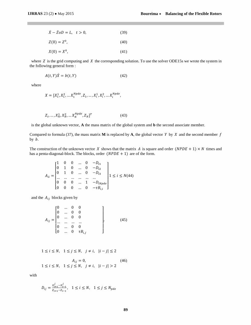
The construction of the unknown vector 𝑋 shows that the matrix 𝐴 is square and order (𝑁𝑃𝐷𝐸 + 1) × 𝑁 times and
has a penta-diagonal-block. The blocks, order (𝑁𝑃𝐷𝐸 + 1) are of the form.
𝐴𝑖𝑖 =
[ 1 0 0 … 0 −𝐷𝑖10 1 0 … 0 −𝐷𝑖20 1 0 … 0 −𝐷𝑖3… … … … … …0 0 0 … 1 −𝐷𝑖𝑁𝑝𝑑𝑒0 0 0 … 0 −𝜏𝐵𝑖,𝑖 ]
1 ≤ 𝑖 ≤ 𝑁(44)
and the 𝐴𝑖𝑗 blocks given by
𝐴𝑖𝑗 =
[ 0 … 0 00 … 0 00 … 0 0… … … …0 … 0 00 … 0 𝜏𝐵𝑖,𝑗 ]
, (45)
1 ≤ 𝑖 ≤ 𝑁, 1 ≤ 𝑗 ≤ 𝑁, 𝑗 ≠ 𝑖, |𝑖 − 𝑗| ≤ 2
𝐴𝑖𝑗 = 0, (46)
1 ≤ 𝑖 ≤ 𝑁, 1 ≤ 𝑗 ≤ 𝑁, 𝑗 ≠ 𝑖, |𝑖 − 𝑗| > 2
with
𝐷𝑖𝑗 =𝑋𝑖+1𝑗−𝑋𝑖−1
𝑗
𝑍𝑖+1−𝑍𝑖−1, 1 ≤ 𝑖 ≤ 𝑁, 1 ≤ 𝑗 ≤ 𝑁𝑝𝑑𝑒
IJRRAS 23 (2) ● May 2015 Boureima ● Balancing of the Flexible Rotors
90
and
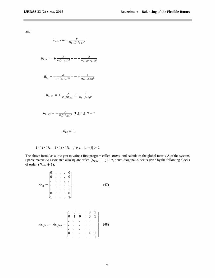
𝐵𝑖,𝑖−2 = −𝜇
𝑀𝑖−1(𝛥𝑍𝑖−2)2
𝐵𝑖,𝑖−1 = +𝜇
𝑀𝑖(𝛥𝑍𝑖−1)2 +⋯+
𝜇
𝑀𝑖−1(𝛥𝑍𝑖−2)2
𝐵𝑖,𝑖 = −𝜇
𝑀𝑖(𝛥𝑍𝑖−1)2 +⋯+
𝜇
𝑀𝑖−1(𝛥𝑍𝑖)2
𝐵𝑖,𝑖+1 = +𝜇
𝑀𝑖(𝛥𝑍𝑖+1)2 +
𝜇
𝑀𝑖−1(𝛥𝑍𝑖)2
𝐵𝑖,𝑖+2 = −𝜇
𝑀𝑖(𝛥𝑍𝑖+1)2 3 ≤ 𝑖 ≤ 𝑁 − 2
𝐵𝑖,𝑗 = 0,
1 ≤ 𝑖 ≤ 𝑁, 1 ≤ 𝑗 ≤ 𝑁, 𝑗 ≠ 𝑖, |𝑖 − 𝑗| > 2
The above formulas allow you to write a first program called 𝑚𝑎𝑠𝑠 and calculates the global matrix A of the system.
Sparse matrix As associated also square order (𝑁𝑝𝑑𝑒 + 1) × 𝑁, penta-diagonal-block is given by the following blocks
of order (𝑁𝑝𝑑𝑒 + 1).
𝐴𝑠𝑖𝑖 =
[ 0 . . . 00 . . . 0. . . . .. . . . .. . . . .0 . . . 01 . . . 1]
, (47)
𝐴𝑠𝑖,𝑖−1 = 𝐴𝑠𝑖,𝑖+1 =
[ 1 0 . . 0 10 1 0 . 0 1. . . . .. . . . .. . . . .0 . . . 1 11 . . . . 1 ]
, (48)
IJRRAS 23 (2) ● May 2015 Boureima ● Balancing of the Flexible Rotors
91
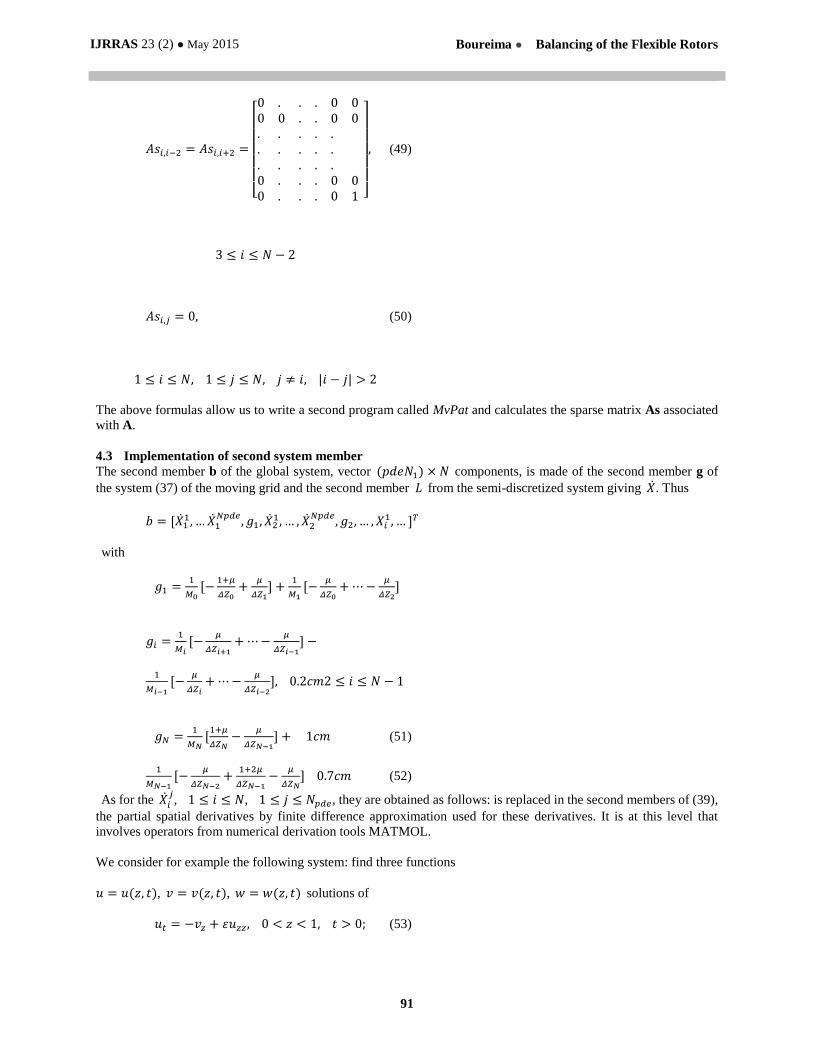
𝐴𝑠𝑖,𝑖−2 = 𝐴𝑠𝑖,𝑖+2 =
[ 0 . . . 0 00 0 . . 0 0. . . . .. . . . .. . . . .0 . . . 0 00 . . . 0 1 ]
, (49)
3 ≤ 𝑖 ≤ 𝑁 − 2
𝐴𝑠𝑖,𝑗 = 0, (50)
1 ≤ 𝑖 ≤ 𝑁, 1 ≤ 𝑗 ≤ 𝑁, 𝑗 ≠ 𝑖, |𝑖 − 𝑗| > 2
The above formulas allow us to write a second program called MvPat and calculates the sparse matrix As associated
with A.
4.3 Implementation of second system member
The second member b of the global system, vector (𝑝𝑑𝑒𝑁1) × 𝑁 components, is made of the second member g of
the system (37) of the moving grid and the second member 𝐿 from the semi-discretized system giving �̇�. Thus
𝑏 = [�̇�11, … �̇�1
𝑁𝑝𝑑𝑒, 𝑔1, �̇�2
1, … , �̇�2𝑁𝑝𝑑𝑒
, 𝑔2, … , 𝑋𝑖1, … ]𝑇
with
𝑔1 =1
𝑀0[−
1+𝜇
𝛥𝑍0+
𝜇
𝛥𝑍1] +
1
𝑀1[−
𝜇
𝛥𝑍0+⋯−
𝜇
𝛥𝑍2]
𝑔𝑖 =1
𝑀𝑖[−
𝜇
𝛥𝑍𝑖+1+⋯−
𝜇
𝛥𝑍𝑖−1] −
1
𝑀𝑖−1[−
𝜇
𝛥𝑍𝑖+⋯−
𝜇
𝛥𝑍𝑖−2], 0.2𝑐𝑚2 ≤ 𝑖 ≤ 𝑁 − 1
𝑔𝑁 =1
𝑀𝑁[1+𝜇
𝛥𝑍𝑁−
𝜇
𝛥𝑍𝑁−1] + 1𝑐𝑚 (51)
1
𝑀𝑁−1[−
𝜇
𝛥𝑍𝑁−2+
1+2𝜇
𝛥𝑍𝑁−1−
𝜇
𝛥𝑍𝑁] 0.7𝑐𝑚 (52)
As for the �̇�𝑖𝑗, 1 ≤ 𝑖 ≤ 𝑁, 1 ≤ 𝑗 ≤ 𝑁𝑝𝑑𝑒, they are obtained as follows: is replaced in the second members of (39),
the partial spatial derivatives by finite difference approximation used for these derivatives. It is at this level that
involves operators from numerical derivation tools MATMOL.
We consider for example the following system: find three functions
𝑢 = 𝑢(𝑧, 𝑡), 𝑣 = 𝑣(𝑧, 𝑡), 𝑤 = 𝑤(𝑧, 𝑡) solutions of
𝑢𝑡 = −𝑣𝑧 + 𝜀𝑢𝑧𝑧, 0 < 𝑧 < 1, 𝑡 > 0; (53)
IJRRAS 23 (2) ● May 2015 Boureima ● Balancing of the Flexible Rotors
92
𝑣𝑡 = −∂
∂𝑧[(𝛾 − 1)𝑤 − 0.5(𝛾 − 3)
𝑣2
𝑢] + (54)
𝜀𝑣𝑧𝑧 , 0 < 𝑧 < 1, 𝑡 > 0;
𝑤𝑡 = −∂
∂𝑧[(𝛾𝑤 − 0.5(𝛾 − 1)
𝑣2
𝑢)𝑣
𝑢] + (55)
𝜀𝑤𝑧𝑧 , 0 < 𝑧 < 1, 𝑡 > 0;
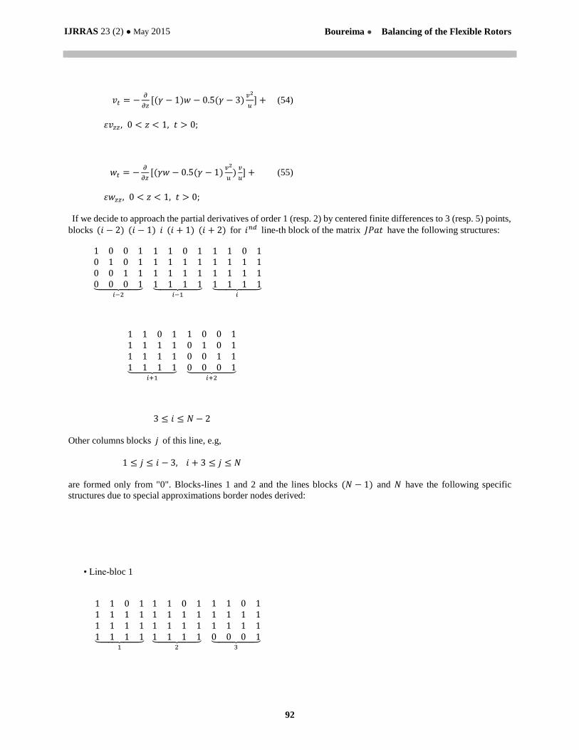
If we decide to approach the partial derivatives of order 1 (resp. 2) by centered finite differences to 3 (resp. 5) points,
blocks (𝑖 − 2) (𝑖 − 1) 𝑖 (𝑖 + 1) (𝑖 + 2) for 𝑖𝑛𝑑 line-th block of the matrix 𝐽𝑃𝑎𝑡 have the following structures:
1 0 0 10 1 0 10 0 1 10 0 0 1⏟
𝑖−2
1 1 0 11 1 1 11 1 1 11 1 1 1⏟
𝑖−1
1 1 0 11 1 1 11 1 1 11 1 1 1⏟
𝑖
1 1 0 11 1 1 11 1 1 11 1 1 1⏟
𝑖+1
1 0 0 10 1 0 10 0 1 10 0 0 1⏟
𝑖+2
3 ≤ 𝑖 ≤ 𝑁 − 2
Other columns blocks 𝑗 of this line, e.g,
1 ≤ 𝑗 ≤ 𝑖 − 3, 𝑖 + 3 ≤ 𝑗 ≤ 𝑁
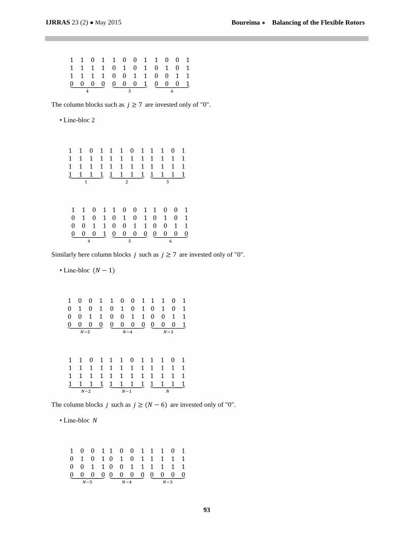
are formed only from "0". Blocks-lines 1 and 2 and the lines blocks (𝑁 − 1) and 𝑁 have the following specific
structures due to special approximations border nodes derived:
• Line-bloc 1
1 1 0 11 1 1 11 1 1 11 1 1 1⏟
1
1 1 0 11 1 1 11 1 1 11 1 1 1⏟
2
1 1 0 11 1 1 11 1 1 10 0 0 1⏟
3
IJRRAS 23 (2) ● May 2015 Boureima ● Balancing of the Flexible Rotors
93
1 1 0 11 1 1 11 1 1 10 0 0 0⏟
4
1 0 0 10 1 0 10 0 1 10 0 0 1⏟
5
1 0 0 10 1 0 10 0 1 10 0 0 1⏟
6
The column blocks such as 𝑗 ≥ 7 are invested only of "0".
• Line-bloc 2
1 1 0 11 1 1 11 1 1 11 1 1 1⏟
1
1 1 0 11 1 1 11 1 1 11 1 1 1⏟
2
1 1 0 11 1 1 11 1 1 11 1 1 1⏟
3
1 1 0 10 1 0 10 0 1 10 0 0 1⏟
4
1 0 0 10 1 0 10 0 1 10 0 0 0⏟
5
1 0 0 10 1 0 10 0 1 10 0 0 0⏟
6
Similarly here column blocks 𝑗 such as 𝑗 ≥ 7 are invested only of "0".
• Line-bloc (𝑁 − 1)
1 0 0 10 1 0 10 0 1 10 0 0 0⏟
𝑁−5
1 0 0 10 1 0 10 0 1 10 0 0 0⏟
𝑁−4
1 1 0 10 1 0 10 0 1 10 0 0 1⏟
𝑁−3
1 1 0 11 1 1 11 1 1 11 1 1 1⏟
𝑁−2
1 1 0 11 1 1 11 1 1 11 1 1 1⏟
𝑁−1
1 1 0 11 1 1 11 1 1 11 1 1 1⏟
𝑁
The column blocks 𝑗 such as 𝑗 ≥ (𝑁 − 6) are invested only of "0".
• Line-bloc 𝑁
1 0 0 10 1 0 10 0 1 10 0 0 0⏟
𝑁−5
1 0 0 10 1 0 10 0 1 10 0 0 0⏟
𝑁−4
1 1 0 11 1 1 11 1 1 10 0 0 0⏟
𝑁−3
IJRRAS 23 (2) ● May 2015 Boureima ● Balancing of the Flexible Rotors
94
1 1 0 11 1 1 11 1 1 10 0 0 1⏟
𝑁−2
1 1 0 11 1 1 11 1 1 11 1 1 1⏟
𝑁−1
1 1 0 11 1 1 11 1 1 11 1 1 1⏟
𝑁
Similarly here column blocks 𝑗 such as 𝑗 ≥ (𝑁 − 6) are invested only of "0".
5. NUMERICAL EXPERIMENTS
5.1 A methanisation in a reactor problem
5.1.1 Description of the problem
A fixed bed reactor is considered wherein the hydrogenation of small amounts methane gives 𝐶𝑂2, according to
chemical equation.
𝐶𝑂2 + 4𝐻2 → 𝐶𝐻4 + 2𝐻2𝑂
Hydrogen was injected into the reactor initially supplied with carbon dioxide following a stepwise pattern. The initial
temperature of the reactor is also adjusted stepwise and we study the evolution of the concentration of carbon dioxide
and evolution of the temperature during the experiment, [7, 8].
Mathematically, the problem is to determine two functions 𝐶 = 𝐶(𝑧, 𝑡) and 𝑇 = 𝑇(𝑧, 𝑡) solutions of
𝐶𝑡 = −𝑣𝐶𝑧 + 𝐷𝐶𝑧𝑧 − 𝑟, 0 < 𝑧 < 𝐿, 𝑡 > 0;(56)
𝑇𝑡 = −𝜀𝑣𝜌𝑔𝑐𝑝𝑔
𝜌𝑐𝑝𝑇𝑧 +
𝜆
𝜌𝑐𝑝𝑇𝑧𝑧 +
2𝑘𝑤
𝑑𝜌𝑐𝑝(𝑇𝑤 − 𝑇) +
(−𝛥𝐻)
𝜌𝑐𝑝𝑟, (57)
0 < 𝑧 > 𝐿, 𝑡 > 0;
where 𝑐(𝑘𝑚𝑜𝑙/𝑚3) is the concentration of reactive species, 𝑇(𝐾) the temperature, 𝐷 = 5 × 10⁻³𝑚2/𝑠 the
diffusivity constant, 𝑣 = 1𝑚/𝑠 the gas velocity, 𝑘 = 29732𝑠−1 the rate constant, 𝐸/𝑅 = 8000𝐾 the activation
temperature, 𝜌𝑐�̅� = 400𝑘𝐽/(𝑚3𝐾) the heat capacity of the fixed bed, 𝜆 = 2.06 × 10⁻³𝑘𝑊/(𝑚𝐾) the effective
axial heat conductivity, 𝜌𝑔𝑐𝑝𝑔 = 0.5𝑘𝐽/(𝑚3𝐾) the heat capacity of the gas, 𝜀 = 0.8 the bed void fraction,
(−𝛥𝐻𝑅) = 206000𝑘𝐽/𝑘𝑚𝑜𝑙 the heat of reaction, 𝐿 = 1𝑚 the reactor length, [8].
For weakly exothermic reactions, operation of the fixed-bed catalytic reactor with periodic flow reversals is of
particular interest. This way, the front and end parts of the catalyst bed act as regenerative heat exchangers for feed
and effluent, allowing the reactions to be operated autothermally at high temperatures. After a start-up phase (here
𝑡𝑠𝑡𝑎𝑟𝑡 = 1500𝑠), where the gas enters at high temperature (𝑐𝑖𝑛 = 1.21 × 10⁻⁴𝑘𝑚𝑜𝑙/𝑚3 at 𝑇𝑖𝑛 = 873𝐾), the feed
temperature is decreased (𝑇𝑖𝑛 = 293𝐾) and periodic flow reversal allows the reactor to be operated autothermally,
[10, 11].
𝐶(𝑧, 0) = 𝐶0(𝑧) = 0, 0 < 𝑧 < 𝐿; (58)
𝑇(𝑧, 0) = 𝑇0(𝑧) = 300, 0 < 𝑧 < 𝐿; (59)
𝐶𝑧(0, 𝑡) =𝑣
𝐷(𝐶 − 𝐶𝑖𝑛), 𝑡 > 0; (60)
IJRRAS 23 (2) ● May 2015 Boureima ● Balancing of the Flexible Rotors
95
𝐶𝑧(𝐿, 𝑡) = 0, 𝑡 > 0; (61)
𝑇𝑧(0, 𝑡) = 𝜀𝑣𝜌𝑔𝑐𝑝𝑔
𝜆(𝑇 − 𝑇𝑖𝑛), 𝑡 > 0; (62)
𝑇𝑧(𝐿, 𝑡) = 0, 𝑡 > 0; (63)
where the reaction rate is given by
𝑟 = 𝑘𝑟𝐶𝑒𝑥𝑝(−
𝐸
𝑅𝑇)
1+𝑘𝑐𝐶;
the initial concentration 𝐶𝑖𝑛 of 𝐶𝑂2 varies by level,
𝐶𝑖𝑛(𝑡) = 0 → 2.5 𝑚𝑜𝑙𝑒𝑠;
The initial temperature 𝑇𝑖𝑛 varies also by level,
𝑇𝑖𝑛(𝑡) = 300 → 500𝐾.
and periodic changes in the sign of the gas velocity 𝑣. From a numerical point of view, this requires the use of
appropriate differentiation matrix.
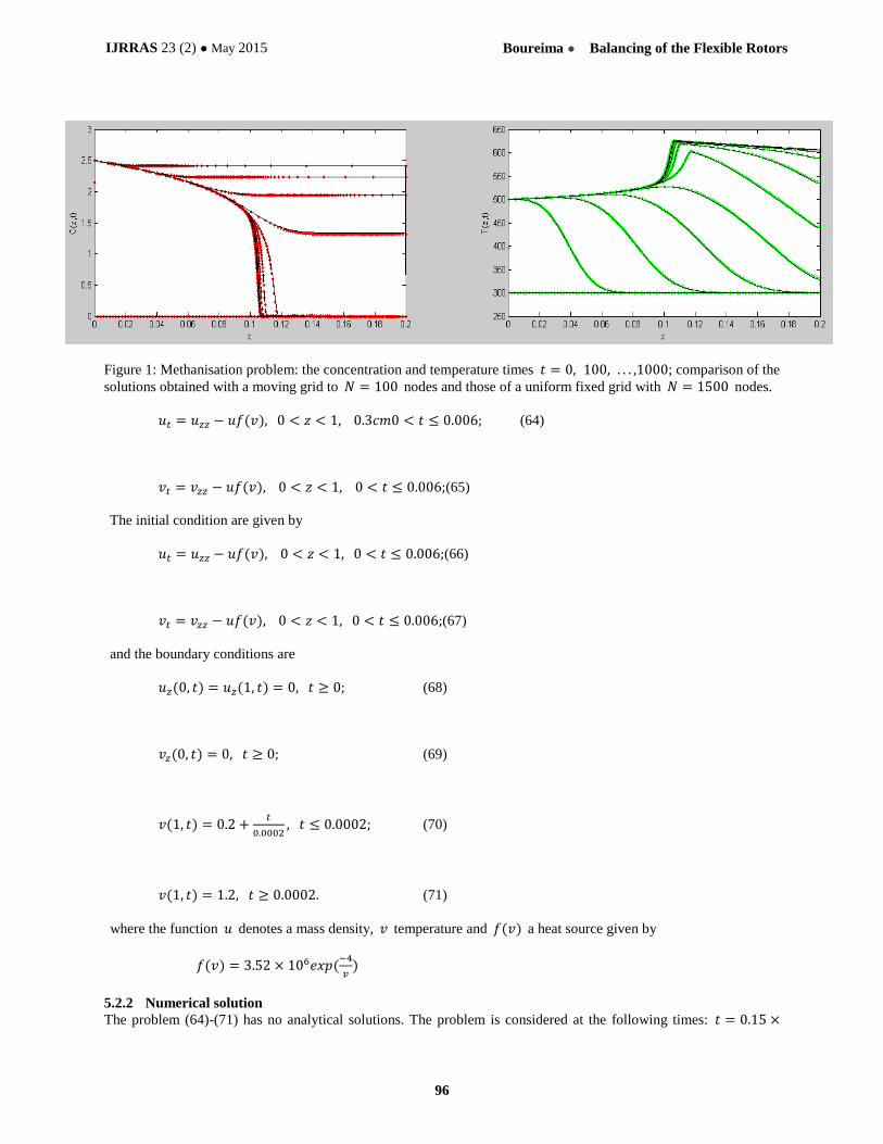
5.1.2 Numerical solution
The problem has no analytical solutions. Reference solution can be computed on a fixed uniform grid with 𝑁 = 1500
nodes.
Figure 1 show the evolution of the concentration and temperature at 𝑡 = 0,100, … ,1000 . Time integration is
performed using the solver 𝑜𝑑𝑒15𝑠 with 𝑅𝑒𝑙𝑇𝑜𝑙 = 10−3 and 𝐴𝑏𝑠𝑇𝑜𝑙 = 10−6. The elements of the concentration
and temperature vectors are interlaced so as to confer a banded structure to the Jacobian matrix, which can be specified
using a function JPattern.
The best results were obtained with the following choice of moving grid parameters and digital derivation operators:
𝛼 = 1, 𝜅 = 2, 𝜏 = 10−2, 𝐷1 = 𝑓𝑜𝑢𝑟 − 𝑝𝑜𝑖𝑛𝑡 − 𝑏𝑖𝑎𝑠𝑒𝑑 − 𝑢𝑝𝑤𝑖𝑛𝑑 and
𝐷2 = 𝑡ℎ𝑟𝑒𝑒 − 𝑝𝑜𝑖𝑛𝑡 − 𝑐𝑒𝑛𝑡𝑒𝑟𝑒𝑑.
For approximating the derivatives of order 1 we used finite differences to four points biased and downstream
derivatives of order 2 centered finite differences to 3 points, [7].
The numerical results obtained with a grate 𝑁 = 100 compared points to those of a fixed uniform grid, even at 𝑁 =1500 nodes show a very good precision numerical solutions with a gain in computing time of the order of 12.8
(427,141 seconds against 5 458.7 seconds).
5.2 A model of flame Propagation
5.2.1 Problem description
Our second example is a model of flame propagation consisting of two coupled equations for mass density and
temperature. This is a problem that simulates several characteristics of flame propagation. A heat source gives rise to
a flame immediately two steep wave fronts propagate in opposite directions, one representing the mass density and
the other temperature [8, 10, 11]. The problem of flame propagation was also discussed in [3].
The problem consists of a system of two partial differential equations (PDEs) supplemented by initial conditions (ICs)
and boundary conditions (BCs). Specifically, it is determined two functions 𝑢 = 𝑢(𝑧, 𝑡) and 𝑣 = 𝑣(𝑧, 𝑡) solutions:
IJRRAS 23 (2) ● May 2015 Boureima ● Balancing of the Flexible Rotors
96
Figure 1: Methanisation problem: the concentration and temperature times 𝑡 = 0, 100, . . . ,1000; comparison of the
solutions obtained with a moving grid to 𝑁 = 100 nodes and those of a uniform fixed grid with 𝑁 = 1500 nodes.
𝑢𝑡 = 𝑢𝑧𝑧 − 𝑢𝑓(𝑣), 0 < 𝑧 < 1, 0.3𝑐𝑚0 < 𝑡 ≤ 0.006; (64)
𝑣𝑡 = 𝑣𝑧𝑧 − 𝑢𝑓(𝑣), 0 < 𝑧 < 1, 0 < 𝑡 ≤ 0.006;(65)
The initial condition are given by
𝑢𝑡 = 𝑢𝑧𝑧 − 𝑢𝑓(𝑣), 0 < 𝑧 < 1, 0 < 𝑡 ≤ 0.006;(66)
𝑣𝑡 = 𝑣𝑧𝑧 − 𝑢𝑓(𝑣), 0 < 𝑧 < 1, 0 < 𝑡 ≤ 0.006;(67)
and the boundary conditions are
𝑢𝑧(0, 𝑡) = 𝑢𝑧(1, 𝑡) = 0, 𝑡 ≥ 0; (68)
𝑣𝑧(0, 𝑡) = 0, 𝑡 ≥ 0; (69)
𝑣(1, 𝑡) = 0.2 +𝑡
0.0002, 𝑡 ≤ 0.0002; (70)
𝑣(1, 𝑡) = 1.2, 𝑡 ≥ 0.0002. (71)
where the function 𝑢 denotes a mass density, 𝑣 temperature and 𝑓(𝑣) a heat source given by
𝑓(𝑣) = 3.52 × 10⁶𝑒𝑥𝑝(−4
𝑣)
5.2.2 Numerical solution
The problem (64)-(71) has no analytical solutions. The problem is considered at the following times: 𝑡 = 0.15 ×
IJRRAS 23 (2) ● May 2015 Boureima ● Balancing of the Flexible Rotors
97
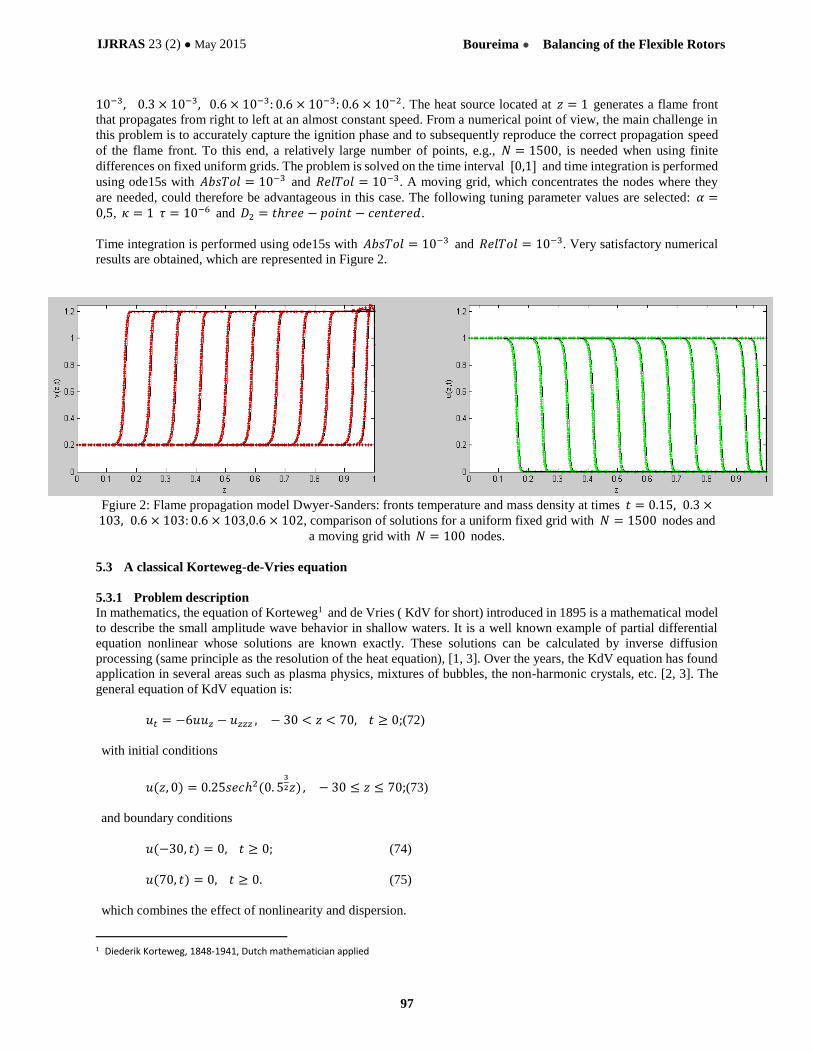
10−3, 0.3 × 10⁻³, 0.6 × 10⁻³: 0.6 × 10⁻³: 0.6 × 10⁻². The heat source located at 𝑧 = 1 generates a flame front
that propagates from right to left at an almost constant speed. From a numerical point of view, the main challenge in
this problem is to accurately capture the ignition phase and to subsequently reproduce the correct propagation speed
of the flame front. To this end, a relatively large number of points, e.g., 𝑁 = 1500, is needed when using finite
differences on fixed uniform grids. The problem is solved on the time interval [0,1] and time integration is performed
using ode15s with 𝐴𝑏𝑠𝑇𝑜𝑙 = 10−3 and 𝑅𝑒𝑙𝑇𝑜𝑙 = 10−3. A moving grid, which concentrates the nodes where they
are needed, could therefore be advantageous in this case. The following tuning parameter values are selected: 𝛼 =0,5, 𝜅 = 1 𝜏 = 10−6 and 𝐷2 = 𝑡ℎ𝑟𝑒𝑒 − 𝑝𝑜𝑖𝑛𝑡 − 𝑐𝑒𝑛𝑡𝑒𝑟𝑒𝑑.
Time integration is performed using ode15s with 𝐴𝑏𝑠𝑇𝑜𝑙 = 10−3 and 𝑅𝑒𝑙𝑇𝑜𝑙 = 10−3. Very satisfactory numerical
results are obtained, which are represented in Figure 2.
Fgiure 2: Flame propagation model Dwyer-Sanders: fronts temperature and mass density at times 𝑡 = 0.15, 0.3 ×10³, 0.6 × 10³: 0.6 × 103,0.6 × 102, comparison of solutions for a uniform fixed grid with 𝑁 = 1500 nodes and
a moving grid with 𝑁 = 100 nodes.
5.3 A classical Korteweg-de-Vries equation
5.3.1 Problem description
In mathematics, the equation of Korteweg1 and de Vries ( KdV for short) introduced in 1895 is a mathematical model
to describe the small amplitude wave behavior in shallow waters. It is a well known example of partial differential
equation nonlinear whose solutions are known exactly. These solutions can be calculated by inverse diffusion
processing (same principle as the resolution of the heat equation), [1, 3]. Over the years, the KdV equation has found
application in several areas such as plasma physics, mixtures of bubbles, the non-harmonic crystals, etc. [2, 3]. The
general equation of KdV equation is:
𝑢𝑡 = −6𝑢𝑢𝑧 − 𝑢𝑧𝑧𝑧 , − 30 < 𝑧 < 70, 𝑡 ≥ 0;(72)
with initial conditions
𝑢(𝑧, 0) = 0.25𝑠𝑒𝑐ℎ2(0. 53
2𝑧) , − 30 ≤ 𝑧 ≤ 70;(73)
and boundary conditions
𝑢(−30, 𝑡) = 0, 𝑡 ≥ 0; (74)
𝑢(70, 𝑡) = 0, 𝑡 ≥ 0. (75)
which combines the effect of nonlinearity and dispersion.
1 Diederik Korteweg, 1848-1941, Dutch mathematician applied
IJRRAS 23 (2) ● May 2015 Boureima ● Balancing of the Flexible Rotors
98
𝑢(𝑧, 𝑡) = 0.5𝑠𝑠𝑒𝑐ℎ2[0.5√(𝑠)(𝑧 − 𝑠𝑡)], (76)
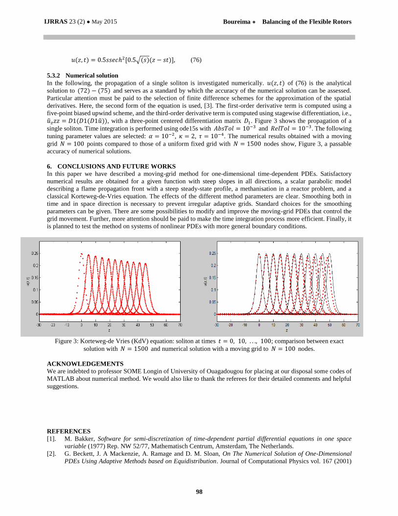
5.3.2 Numerical solution
In the following, the propagation of a single soliton is investigated numerically. 𝑢(𝑧, 𝑡) of (76) is the analytical
solution to (72) − (75) and serves as a standard by which the accuracy of the numerical solution can be assessed.
Particular attention must be paid to the selection of finite difference schemes for the approximation of the spatial
derivatives. Here, the second form of the equation is used, [3]. The first-order derivative term is computed using a
five-point biased upwind scheme, and the third-order derivative term is computed using stagewise differentiation, i.e.,
�̃�𝑧𝑧𝑧 = 𝐷1(𝐷1(𝐷1�̃�)), with a three-point centered differentiation matrix 𝐷1. Figure 3 shows the propagation of a
single soliton. Time integration is performed using ode15s with 𝐴𝑏𝑠𝑇𝑜𝑙 = 10−3 and 𝑅𝑒𝑙𝑇𝑜𝑙 = 10−3. The following
tuning parameter values are selected: 𝛼 = 10−2, 𝜅 = 2, 𝜏 = 10−4. The numerical results obtained with a moving
grid 𝑁 = 100 points compared to those of a uniform fixed grid with 𝑁 = 1500 nodes show, Figure 3, a passable
accuracy of numerical solutions.
6. CONCLUSIONS AND FUTURE WORKS
In this paper we have described a moving-grid method for one-dimensional time-dependent PDEs. Satisfactory
numerical results are obtained for a given function with steep slopes in all directions, a scalar parabolic model
describing a flame propagation front with a steep steady-state profile, a methanisation in a reactor problem, and a
classical Korteweg-de-Vries equation. The effects of the different method parameters are clear. Smoothing both in
time and in space direction is necessary to prevent irregular adaptive grids. Standard choices for the smoothing
parameters can be given. There are some possibilities to modify and improve the moving-grid PDEs that control the
grid movement. Further, more attention should be paid to make the time integration process more efficient. Finally, it
is planned to test the method on systems of nonlinear PDEs with more general boundary conditions.
Figure 3: Korteweg-de Vries (KdV) equation: soliton at times 𝑡 = 0, 10, . . ., 100; comparison between exact
solution with 𝑁 = 1500 and numerical solution with a moving grid to 𝑁 = 100 nodes.
ACKNOWLEDGEMENTS
We are indebted to professor SOME Longin of University of Ouagadougou for placing at our disposal some codes of
MATLAB about numerical method. We would also like to thank the referees for their detailed comments and helpful
suggestions.
REFERENCES [1]. M. Bakker, Software for semi-discretization of time-dependent partial differential equations in one space
variable (1977) Rep. NW 52/77, Mathematisch Centrum, Amsterdam, The Netherlands.
[2]. G. Beckett, J. A Mackenzie, A. Ramage and D. M. Sloan, On The Numerical Solution of One-Dimensional
PDEs Using Adaptive Methods based on Equidistribution. Journal of Computational Physics vol. 167 (2001)
IJRRAS 23 (2) ● May 2015 Boureima ● Balancing of the Flexible Rotors
99
pp. 372-392.
[3]. A. Jeffrey and S. Xu, Exact solutions to the Korteweg-de Vries-Burgers Equation, Wave Motion, 11(1989)
559-564.
[4]. A. Kurganov and E. Tadmor. New high-resolution central schemes for nonlinear conservation laws and
convection-diffusion equations. Journal of Computational Physics, 160:241-282, 2000.
[5]. N. Maman, Algorithmes d’adaptation dynamique de maillages en éléments finis. Application à des
écoulements réactifs instationnaires, PhD thesis, Université Paul Sabatier de Toulouse, 1992.
[6]. B. Sangaré, O. Diallo and L. Somé, A New MATLAB Implementation and Analysis of A Moving Grid
Method For Systems of One-Dimensional Time-Dependent Partial Differential Equations Based on The
Equidistribution Principle, Int. J. Appl. Math. 25(2012), no.1, 66-85.
[7]. A. Vande Wouwer, P. Saucez ,W. E. Schiesser, S. Thompson, A MATLAB implementation of upwind finite
differences and adaptive grids in the method of lines Journal of Computational and Applied Mathematics 183
(2005) 245–258.
[8]. W.E. Schiesser, The Numerical Method of Lines: Integration of Partial Differential Equations, Academic Press,
San Diego, 1991.
[9]. P. Saucez, L. Some and A. Vande Wouwer Matlab Implementation of a Moving Grid Method based on the
Equidistribution Principle Fourth International Conference on Advanced COmputational Methods in
ENgineering (ACOMEN 2008)
[10]. A. Vande Wouwer, Ph. Saucez, and W.E. Schiesser. Simulation of distributed parameter systems using a
matlab-based method of lines toolbox-chemical engineering applications. Industrial Engineering and
Chemistry Research, 43:3469–3477, 2004.
[11]. Verwer, J.G, Blom, R.M. Furzeland, P. A. Zegeling, A moving grid method for one-dimensional PDEs based
on the method of lines. In Adaptive methods for Partial Differential Equations, J.E. Flaherty, P.J. Paslow, M.S.
Shepard, and J.D. Vasilakis (Eds.), SIAM, Philadelphia, Pa., (1989) 160-175.
[12]. P. A. Zegeling, Moving grid methods for time-dependent partial differential equations, CWI TRACT 94 (1993),
47-60 and 92-95.