finite element analysis of 3d-model of turning tables...

ACTA TEHNICA CORVINIENSIS – Bulletin of Engineering Tome VIII [2015] Fascicule 4 [October – December]

ISSN: 2067 – 3809

© copyright Faculty of Engineering - Hunedoara, University POLITEHNICA Timisoara

1. Ibraheem A. SAMOTU, 2. Fatai O. ANAFI, 3. Muhammad DAUDA, 4. Abdulkarim S. AHMED, 5. Raymond B. BAKO, 6. David .O. OBADA

FINITE ELEMENT ANALYSIS OF 3D-MODEL OF TURNING TABLES OF MICRO-CONTROLLER BASED VERSATILE

MACHINE TOOLS DESKTOP LEARNING MODULE

1-3,6 .Department of Mechanical Engineering, Ahmadu Bello University, Zaria, NIGERIA 4 .Department of Chemical Engineering, Ahmadu Bello University, Zaria, NIGERIA

5. Department of Education Foundations and Curriculum, Ahmadu Bello University, Zaria, NIGERIA

Abstract: In this paper, we present the results of finite element analysis (FEA) performed to investigate nature of stress and their distribution at optimum point along the two turning tables of a micro-controller based versatile machine tool desktop learning module. Commercial Autodesk Inventor was used to create both three-dimensional (3-D) and 2-D models as well as performing simulation. Dynamics simulation generated the motion load expected to act on the tables when used for real-life operation which were in turn used to perform FEA. The motion of the dc servo motor driving the tables and other parts of the module is designed to be controlled by programmable chips. Before creating FEA simulation for the tables, numerical divergence were prevented by varying the mesh settings to obtain the settings at which the results of the analyses converges which was obtained at 0.03 average element size and 0.04 minimum element size. Finite element analysis carried out on the tables shows that aluminium alloy 4032-T6 chosen will serve in the fabrication of physical prototype. FEA revealed the nature and level of stresses that will be experienced on the tables, it also revealed region where these stresses will concentrate on them. The analysis also estimated the expected weight of the turning tables 1&2 to be 1.23536 to 0.257182 Kg respectively and show that the minimum factor of safety was constantly 15 ul within the tables which shows that they will not fail during operation. Keywords: Turning table, Lathe, Machine Tools, Stress, Displacement, Factor of Safety

INTRODUCTION Turning is one of the most common of metal cutting operations. In turning, a workpiece is rotated about its axis as single-point cutting tools are fed into it, shearing away unwanted material and creating the desired part. Turning can occur on both external and internal surfaces to produce an axially-symmetrical contoured part. Turning is an engineering machining process in which a cutting tool, typically a non-rotary tool bit, describes a helical tool-path by moving more or less linearly while the workpiece rotates. [1] The tool's axes of movement may be literally a straight line, or they may be along some set of curves or angles, but they are essentially linear (in the nonmathematical sense). Usually the term "turning" is reserved for the generation of external surfaces by this cutting action, whereas this same essential cutting action when applied to internal surfaces (that is, holes, of one kind or another) is called "boring". Thus the phrase "turning and boring" categorizes the larger family of (essentially similar) processes. The cutting of faces on the workpiece (that is, surfaces perpendicular to its rotating axis), whether with a turning or boring tool, is called "facing", and may be lumped into either category as a subset [1]. Turning can be done manually, in a traditional form of lathe, which frequently requires continuous supervision by the operator, or by using an automated lathe which does not. Today the most common type of such

automation is computer numerical control, better known as CNC. (CNC is also commonly used with many other types of machining besides turning.) This operation is one of the most basic machining processes. That is, the part is rotated while a single point cutting tool is moved parallel to the axis of rotation [2]. Turning can be done on the external surface of the part as well as internally (boring). The starting material is generally a workpiece generated by other processes such as casting, forging, extrusion, or drawing. The idea of cooperative hands-on active problem-based learning (CHAPL) using desktop learning module (DLM) involves grouping students into home teams (3-5) to complete homework, in class worksheets and projects. Class time itself consists of teams completing worksheets that require hands on use of physical models and active data collection. The focus is always on giving students an active role in their own education in a way to implement Kolb’s experimental model (see Plate 1) in a non-lab class using physical models. [3]. Flashlight Survey was conducted on Nigerian students who were taught with hands-on active learning (HAL) pedagogy for a semester by a group of researchers [4]. This was done to assess their own feelings regarding the class experience and utilizes Chickering and Gamson’s seven (7) principles of good practice as a basis for question topics [5].The survey revealed that large number of students felt CHAPL allowed them to

http://en.wikipedia.org/wiki/Lathe

http://en.wikipedia.org/wiki/Machining

http://en.wikipedia.org/wiki/Casting

http://en.wikipedia.org/wiki/Forging

http://en.wikipedia.org/wiki/Extrusion

http://en.wikipedia.org/wiki/Drawing_(manufacturing)

ACTA TEHNICA CORVINIENSIS Fascicule 4 [October – December] – Bulletin of Engineering Tome VIII [2015]

| 44 |

visualize concepts and grasp facts better than a standard lecture. Additionally a significant number of students felt more comfortable in discussions after using the DLMs in a CHAPL setting.

Plate 1. The Kolb Experiential Cycle [3]

It has also been identified that students trained totally with traditional lecture format (TLF) tends to wait to be told about problems and still rely on superiors for direction and information in solving them rather than looking for problems to fix. This happens because TLF typically involves the superior, a professor, telling the students how things are done and what the problems are. If there are any questions, the professor is generally the provider of the ‘correct’ answer. In essence, we are training students to expect this type of knowledge from superiors at workplace [6]. An alternate method of conducting classes is needed if we desire to prepare students to be independent learners who communicate effectively and work well as part of a team. In today’s science and engineering classrooms, passive lecture based teaching is slowly giving way to more well-rounded pedagogies such as POGIL and high performance learning Environment (Hi-PeLE) that incorporate active student participation [7], Motivation for this paradigm shift comes from numerous findings that hands on, active learning possesses advantages over purely aural teaching [8;9]. There are report of existing desktop learning modules (DLMs) which contain a one cubic foot base system with hot and cold fluid reservoirs, flow meters, temperature and pressure readouts and a set of interchangeable unit operations cartridges. They were developed to give students hands-on experience in the selected area [6;10]. Recent efforts to extend the DLM concept to the civil engineering discipline was reported in an article [10], now more concerted effort and rigorous study is taking place in Civil Engineering while expansion to Bio-, Mechanical and Electrical Engineering is underway [11]. Some of the new interchangeable cartridges that are being developed and their utility in terms of concepts and principles that can be learned or reinforced by those using them include Bioengineering Cartridges, Civil Engineering Flume, Misconceptions, and Assessment Strategy, New Chemical Engineering cartridges and Mechanical Engineering Solar Cartridge. Finally, DLM for Machine tool training/teaching is presently not available in this part of the world where resources are limited. This makes it is more difficult to teach this course using problem based learning (PBL) approach because of infrastructural deficiencies such as desktop size machine tool, electricity and workshops. To address this issue, new Desktop Learning Modules (DLMs) that contain miniaturized processes with a uniquely expandable electronic system to

contend with known sensor systems/removable cartridges were designed. This is expected to be a miniaturized mimics of industrial-scale equipment that will produce process data that agree with correlations developed for large-scale equipment. Therefore, this article discusses details of modelling and finite element analysis carried out on the turning tables of the designed machine tools desktop learning module (MT-DLM) before developing a physical prototype for cooperative, hands on, active and problem based learning (CHAPL) of turning and related operations which can be done on a lathe in Nigerian higher institutions.

INVENTOR ASSEMBLIESConstrained Completely or partially

START DYNAMICS SIMULATION

AUTOMATICALLY CONVERT CONSTRAINTS TO JOINTS

MANUALLY CREATE MORE SPECIFIC JOINTS=Springs/Actuators/2D Contacts etc

CHECK FOR REDUNDANT JOINTS AND FIX

CREATE ENVIRONMENTAL CONSTRAINTS-Initial Positions/Imposed Motions/Forces/Friction/Gravity etc

RUN THE DYNAMIC SIMULATION

ANALYSE RESULTS FROM THE OUTPUT GRAPHER

MODIFY JOINTS

MODIFY PARTS

MODIFY ENVIRONMENTAL CONSTARAINTS

RUN SIMULATION AGAIN

SUCCESSFUL VIRTUAL SIMULATION

TRANSFER MULTIPLE LOAD TO STRESS ANALYSIS

ANALYSE PARTS

MODIFY PARTS

REANALYZE/OPTIMISE PARTS

RUN AND ANALYSE SIMULATION AGAIN

FINAL OPTIMISED PARTS AND SIMULATION Figure 1. Motion Simulation and FEA Total Workflow Diagram. [20]

There are numerous simulation tool available to designer which include Autodesk Inventor Pro, Solid Works Pro, MATLAB & Simulink, Maple Sim


| 45 |

etc., while simulation environments include Finite Element analysis, Dynamic Simulation, Frame Analysis among others. These tools also allows for designers to test for suitability of newly developed materials for their intended designs before purchasing such materials [12]. This reduces the number of physical prototype required before a final component can be produced there by reducing cost, lead time of production and material waste among other benefits. Lot of research activities that involve the use of finite element analysis on designs with different purposes have been reported, some used it to improve an existing design while some use it to measure the level of stress and deformation expected within a system. [13-19] A recommended motion simulation and FEA total workflow diagram is presented in Figure 1. RESEARCH PROCEDURE Model Creation The 3D-model of the desktop size lathe as it will be used for machining was created using commercial Autodesk Inventor software package. The software allows for dynamics simulation as well as assigning of material for each component part of the module. The main factor considered during the modelling are;

≡ Workpiece Geometry. ≡ Overall weight of the setup. ≡ Ease of casting and machining of the parts. ≡ Availability of the assigned material. ≡ Displacement (Deformation) of the parts. ≡ Factor of safety.

The workpiece geometries that were used for the creation of the models are 100 mm cylindrical rod of diameter 15 mm for turning operation and 100 mm square plate of thickness 25 mm for milling, drilling, planing and grinding operations. Parametric study was conducted on the turning tables with the aim of optimizing the weight and the level of deformation within it. The study aided in reducing the weight of turning table 1 & 2 from 3.85456 kg to 1.28217 Kg and 1.23536 to 0.257182 Kg while the deformation increased from 0.0000925 and 0.00257 μm to a maximum value of 1.04 and 4.97 μm respectively.

Plate 2. Plan of the MT-DLM during Turning Operation

Based on these design considerations, 3D models were created and their 2D Projections are presented in the following plates to show the distance between the spindle jaws and the tip of the tail stock for the turning model and the gap within the locating pins of the milling table.

Plate 3. Front view of the MT-DLM during Milling Operation

Model Simulation The procedure for the simulation carried out on the model followed the recommended total workflow diagram (See Figure 1). Dynamic simulation in Autodesk Inventor Dynamic simulation environment is located under environment tool bar in Autodesk Inventor. The environment automatically generate standard joints within the model based on the kind of constrains placed on each component during assembly while components were also grouped into grounded and mobile members. The environment allows for gravitational force and other kind of forces to be applied on the model which are group under external loads section of the environment. Dynamic Motion sub-tab was used to inspect how the parts moved relatively to each other before the simulation was carried out. After the parts moved satisfactorily in respect of others, the simulation was carried out using the simulation player. The environment automatically generate standard joints within the model based on the kind of constrains placed on each component during assembly while components were also grouped into grounded and mobile members. The environment allows for gravitation force and other kind of forces to be applied on the model which are group under external loads section of the environment. Dynamic Motion sub-tab was used to inspect how the parts moved relatively to each other before the simulation was carried out. After the parts moved satisfactorily in respect of others, the simulation was carried out using the simulation player. Tracers were attached to the two turning tables to monitor only the vector components of change in position and velocity relatively to the ground. The results of the traces were displayed on the Output Grapher of the environment. Prior to the running of the simulation, the tables were exported to the FEA environment as they are expected to experience varying forces due to the change in position and motion during the real life operation of the MT-DLM.


| 46 |

The traced results of the output grapher generated the selected parameter in numerous time steps out of which eleven (11) important time steps including beginning and ending time were automatically exported to the FEA simulation environment. The selected time steps are points where some peaks were found on the output of the output grapher traces. Finite element analysis (FEA) FEA was done based on the motion loads generated from the dynamics simulation environment for the tables which were exported in eleven (11) time steps. Before creating FEA simulation for the tables, numerical divergence were prevented by varying the mesh settings to obtain the settings at which the results of the analyses converges. The average element size as a fraction of model diameter and minimum element size as a fraction of the average element size were varied to obtain the convergence point. The convergence setting for all the exported part was obtained at 0.03 average element size and 0.04 minimum element size which was used to run the simulations. Aluminium 4032-T6 was assigned to the two tables during the simulation. This was done to determine if the selected material can withstand the kind of stresses to be generated during operation. The main factor that was used to determine this was the calculated factor of safety from the simulation result. The yield strength, ultimate tensile strength and density used for the simulation were 315 MPa, 380 MPa and 2.68 g/cm3 respectively. These properties played major role during the simulation. RESULTS AND DISCUSSION This section presents results of the simulations done on the designed model of MT-DLM. Dynamics Simulation The trace obtained from the output grapher is presented in Figure 3 below. In the figure,3, Trace 1 is for turning table 2 while Trace 2 is for turning table 1.

Figure 2. Turning Operation Dynamics Simulation Trace

Discussion of dynamics simulation results The output traces of the dynamics simulation done is presented in Figures 3 above. Dynamics simulations were done to generate the boundary

conditions applied to the tables which were exported to the FEA environment for further simulations. The trace shows that the turning table 2 assembly moved with constant acceleration, given the assembly a uniformly increased speed under a constant torque until it has contact with the milling table attached to the other part of the frame. This is a scenario that must be prevented in the physical prototype fabrication. The contact is expected to give a back-movement of the assembly as the speed falls to negative value, this is expected to affect the surface finish profile of the part the model will be used to machine (See Figure 2). The impact of the contact on the assembly was further investigated during the finite element analysis. The trace also shows that the change in position of the turning table 1 assembly is not linear but parabolic (quadratic) in nature; this is associated with the effect of the turning table 2 assembly attached to it which is moving along another axis perpendicular to its own movement. The speed of the turning table 1 assembly increases at a constant rate with constant acceleration but the effect of the contact of the turning table 2 assembly and the milling table assembly can be seen between 0.5-0.6 s time steps which sharply reduces the speed of the table before the speed continues to increase at the initial rate. Finite element analysis results The variations in the stresses and displacement with time for the tables were measured during the finite element analyses. Some of the values were constant throughout the simulation time-steps while some varies. The constant values are summarized on Table 1 below. Maximum equivalent stress was estimated based on von Mises criterion and recorded as von Mises stress. 1st and 3rd principal stresses, shear and direct stresses as well as their strain and displacement were all estimated during the FEA. The variations of the equivalent stress and displacement with time are presented in the following figures. The distribution of the stress and displacement along the tables was probed at the time step where optimum value was obtained which complements the variation.

Table 1. Constant values obtained from the tables

Name Turning Table 1

Turning Table 1 Cover

Turning Table 2

Mass (Kg) 1.28217 0.460092 0.257182 1st Principal Stress

(MPa) 1.131 1.336 15.26

3rd Principal Stress (MPa) -1.163 -1.385 -14.32

Remote Force 1 (N) 31.098 12.965 152.93 Remote Force 2 (N) 1.733 17.575 12.965 Remote Force 3 (N) 17.575 - 106.439 Moment 1 (N mm) 10226.521 7465.64 62.792 Moment 2 (N mm) 87.02 4770.245 6082.745 Moment 3 (N mm) 4770.245 - 5087.37

The variation in other parameters with time and their distribution are presented in the following figures. Turning table 1 The variation in the von Mises stress and displacement for the turning table 1 is presented in the figures below.

-700.000

-600.000

-500.000

-400.000

-300.000

-200.000

-100.000

0.000

100.000

200.000

300.000

400.000

0 0 . 2 0 . 4 0 . 6 0 . 8 1

TIME ( S )

P[Y] (Trace:1) ( mm ) V[Y] (Trace:1) ( mm/s )

P[X] (Trace:2) ( mm ) V[X] (Trace:2) ( mm/s )


| 47 |

Figure 3a. Variation of Von Mises Stress with Time

Figure 3b. Distribution of Von Mises Stress along the Turning Table 1

Figure 4a. Variation of Displacement with Time

Figure 4b. Distribution of Displacement along the Turning Table 1

Turning Table 1 Cover The variation in the von Mises stress and displacement for the turning table 1 cover is presented in the figures below;


Figure 5b. Distribution of Von Mises Stress along

the Turning Table 1 Cover


Figure 6b. Distribution of Displacement along

the Turning Table 1 Cover

0.9

0.95

1

1.05

1.1

1.15

0 0.2 0.4 0.6 0.8 1

Stre

ss (M

Pa)

Time (s)

0.0007

0.00075

0.0008

0.00085

0.0009

0.00095

0.001

0.00105

0.0011

0 0.2 0.4 0.6 0.8 1

Disp

lace

men

t (m

m)

Time (s)

00.20.40.60.8

11.21.41.6

0 0.2 0.4 0.6 0.8 1

Stre

ss (M

Pa)

Time (s)

00.0005

0.0010.0015

0.0020.0025

0.0030.0035

0.0040.0045

0 0.2 0.4 0.6 0.8 1

Disp

lace

men

t (m

m)

Time (s)


| 48 |

Turning Table 2 The variation in the von Mises stress and displacement for the turning table 2 is presented in the figures below;


Figure 7b. Distribution of Von Mises Stress along the Turning Table 2


Figure 8b. Distribution of Displacement along the Turning Table 2

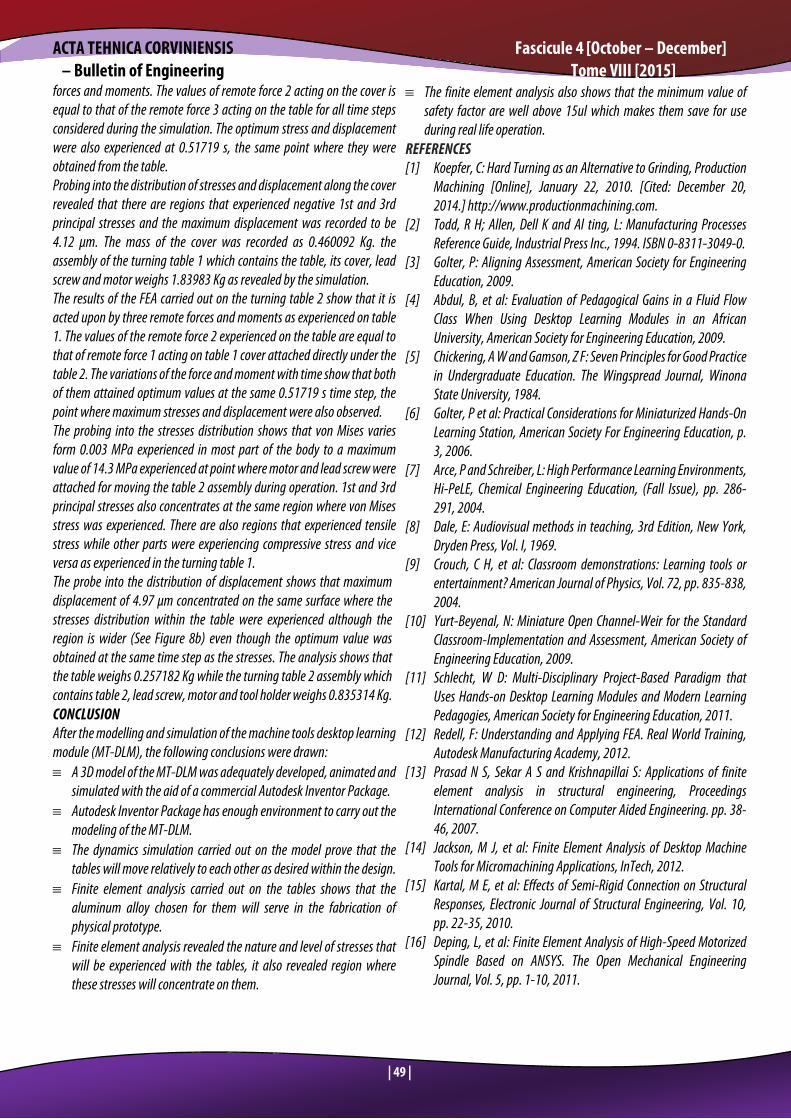
Discussion of Finite Element Analysis Results Finite element analysis carried out on the turning table 1 reveals that three (3) remote forces were acting on the table leading to the generation of three (3) moments which were also acting on it out of which only one moment and one force were constant throughout the simulation time steps. The combination effect of the forces and moments led to the generation of three-dimensional loads which in turn developed the equivalent (von Mises) stress based on von Mises criterion within the table. The variation in the developed von Mises stress with time is presented in Figure 5a while the distribution of the stress at the time step where optimum value was obtained is presented in Figure 5b. The results show that the optimum equivalent stress was obtained at 0.51719 s with a value of 1.113 MPa. This time step is the same as the time when the turning table 2 had contact with the milling table during dynamics simulation. The variations of 1st and 3rd principal stresses follows that of the von Mises stress. The peaks were obtained at the same time step for all the stresses although the values are not the same at those peaks. The probing into the distribution of 1st principal stress shows that there are regions that experienced negative values. This negative value of up to 0.369 MPa implies that there is a compressive stress at those region since the 1st principal stress is expected to account for tensile stress within the body. The same manner, some regions experienced negative 3rd princioal stress, these regions coincide with those that experienced negative 1st principal stress which means they were experiencing tensile stress while other parts of the turning table 1 were experiencing compressive stress and vice versa. This regions are mostly found along the edges of the dove tail where the table is connected to the frame. The variation in the remote forces and moments with time shows that the maximum values for all the remote forces and moments were obtained at the time step where maximum stresses were obtained from the simulation, this implies that the variation of the forces acting on the turning table causes the variation of stresses experienced within the part. The variation of the displacement with time follows the trends observed in all the stresses measured. The displacement accounts for the level of deformation that will be experienced at those region of the analyzed part. Probing into the distribution of displacement along the turning table 1 revealed that maximum deformation will be experienced at the tin edges of the dove tail attached to the table and the surface where the driving motor and lead screw were attached to it. These are the regions where maximum stresses were experienced during the simulation. The maximum level of deformation expected is 1.06 μm, a displacement that is not expected to give any significant influence on the accuracy of the table movement during operation. This is in line with the submission of (16) on the influence of maximum displacement value on accuracy of analyzed part. Finally, the analysis also revealed that turning table 1 weighs 1.28217 Kg The results of the FEA carried out on the cover of turning table show that only two remote forces and moments were acting on it although it was attached directly to the turning table 1 which experienced three remote

02468

10121416

0 0.2 0.4 0.6 0.8 1

Stre

ss (M

Pa)

Time (s)

0

0.001

0.002

0.003

0.004

0.005

0.006

0 0.5 1

Disp

lace

men

t (m

m)

Time (s)


| 49 |

forces and moments. The values of remote force 2 acting on the cover is equal to that of the remote force 3 acting on the table for all time steps considered during the simulation. The optimum stress and displacement were also experienced at 0.51719 s, the same point where they were obtained from the table. Probing into the distribution of stresses and displacement along the cover revealed that there are regions that experienced negative 1st and 3rd principal stresses and the maximum displacement was recorded to be 4.12 μm. The mass of the cover was recorded as 0.460092 Kg. the assembly of the turning table 1 which contains the table, its cover, lead screw and motor weighs 1.83983 Kg as revealed by the simulation. The results of the FEA carried out on the turning table 2 show that it is acted upon by three remote forces and moments as experienced on table 1. The values of the remote force 2 experienced on the table are equal to that of remote force 1 acting on table 1 cover attached directly under the table 2. The variations of the force and moment with time show that both of them attained optimum values at the same 0.51719 s time step, the point where maximum stresses and displacement were also observed. The probing into the stresses distribution shows that von Mises varies form 0.003 MPa experienced in most part of the body to a maximum value of 14.3 MPa experienced at point where motor and lead screw were attached for moving the table 2 assembly during operation. 1st and 3rd principal stresses also concentrates at the same region where von Mises stress was experienced. There are also regions that experienced tensile stress while other parts were experiencing compressive stress and vice versa as experienced in the turning table 1. The probe into the distribution of displacement shows that maximum displacement of 4.97 μm concentrated on the same surface where the stresses distribution within the table were experienced although the region is wider (See Figure 8b) even though the optimum value was obtained at the same time step as the stresses. The analysis shows that the table weighs 0.257182 Kg while the turning table 2 assembly which contains table 2, lead screw, motor and tool holder weighs 0.835314 Kg. CONCLUSION After the modelling and simulation of the machine tools desktop learning module (MT-DLM), the following conclusions were drawn: ≡ A 3D model of the MT-DLM was adequately developed, animated and

simulated with the aid of a commercial Autodesk Inventor Package. ≡ Autodesk Inventor Package has enough environment to carry out the

modeling of the MT-DLM. ≡ The dynamics simulation carried out on the model prove that the

tables will move relatively to each other as desired within the design. ≡ Finite element analysis carried out on the tables shows that the

aluminum alloy chosen for them will serve in the fabrication of physical prototype.

≡ Finite element analysis revealed the nature and level of stresses that will be experienced with the tables, it also revealed region where these stresses will concentrate on them.

≡ The finite element analysis also shows that the minimum value of safety factor are well above 15ul which makes them save for use during real life operation.

REFERENCES [1] Koepfer, C: Hard Turning as an Alternative to Grinding, Production

Machining [Online], January 22, 2010. [Cited: December 20, 2014.] http://www.productionmachining.com.

[2] Todd, R H; Allen, Dell K and Al ting, L: Manufacturing Processes Reference Guide, Industrial Press Inc., 1994. ISBN 0-8311-3049-0.

[3] Golter, P: Aligning Assessment, American Society for Engineering Education, 2009.

[4] Abdul, B, et al: Evaluation of Pedagogical Gains in a Fluid Flow Class When Using Desktop Learning Modules in an African University, American Society for Engineering Education, 2009.

[5] Chickering, A W and Gamson, Z F: Seven Principles for Good Practice in Undergraduate Education. The Wingspread Journal, Winona State University, 1984.

[6] Golter, P et al: Practical Considerations for Miniaturized Hands-On Learning Station, American Society For Engineering Education, p. 3, 2006.

[7] Arce, P and Schreiber, L: High Performance Learning Environments, Hi-PeLE, Chemical Engineering Education, (Fall Issue), pp. 286-291, 2004.

[8] Dale, E: Audiovisual methods in teaching, 3rd Edition, New York, Dryden Press, Vol. I, 1969.

[9] Crouch, C H, et al: Classroom demonstrations: Learning tools or entertainment? American Journal of Physics, Vol. 72, pp. 835-838, 2004.

[10] Yurt-Beyenal, N: Miniature Open Channel-Weir for the Standard Classroom-Implementation and Assessment, American Society of Engineering Education, 2009.

[11] Schlecht, W D: Multi-Disciplinary Project-Based Paradigm that Uses Hands-on Desktop Learning Modules and Modern Learning Pedagogies, American Society for Engineering Education, 2011.

[12] Redell, F: Understanding and Applying FEA. Real World Training, Autodesk Manufacturing Academy, 2012.

[13] Prasad N S, Sekar A S and Krishnapillai S: Applications of finite element analysis in structural engineering, Proceedings International Conference on Computer Aided Engineering. pp. 38-46, 2007.

[14] Jackson, M J, et al: Finite Element Analysis of Desktop Machine Tools for Micromachining Applications, InTech, 2012.

[15] Kartal, M E, et al: Effects of Semi-Rigid Connection on Structural Responses, Electronic Journal of Structural Engineering, Vol. 10, pp. 22-35, 2010.

[16] Deping, L, et al: Finite Element Analysis of High-Speed Motorized Spindle Based on ANSYS. The Open Mechanical Engineering Journal, Vol. 5, pp. 1-10, 2011.


| 50 |

[17] Yung-Chang, Y, et al: Estimation of tool wear in orthogonal cutting using the finite element analysis, Journal of Materials Processing Technology, Vol. 146, pp. 82–91, 2004.

[18] Wakchaure, M R and Sagade, A V: Finite Element Analysis of Castellated Steel Beam, International Journal of Engineering and Innovative Technology (IJEIT), Vol. 2, pp. 365-372, 1, July 2012.

[19] Ali, B A, et al: Finite Element Analysis of Cold-formed Steel Connections, International Journal of Engineering (IJE), Vol. 5, 2011.

[20] Waguespack, C: Mastering Autodesk Inventor 2014 and Autodesk Inventor LT, Indianapolis, Indiana: John Wiley & Sons, Inc., 2014. A book of SYBEX (A Wiley Brand).

copyright ©

University POLITEHNICA Timisoara, Faculty of Engineering Hunedoara,

5, Revolutiei, 331128, Hunedoara, ROMANIA http://acta.fih.upt.ro

finite element analysis of 3d-model of turning tables...

Documents