Finite Element Analysis of the Tape Scanner Interface in Helical Scan Recording

CIP-GEGEVENS KONINKLIJKE BIBLIOTHEEK, DEN HAAG

Rongen, Peter Maria Johannes

Finite element analysis of the tape scanner interface in helical scan recording / Peter Maria Johannes Rongen. -Eindhoven : Philips Natuurkundig Laboratorium. Ill. Thesis Eindhoven. - With ref. ISBN 90-74445-15-2 Subject headings: magnetic recording / finite element analysis / tribology.

On the cover: a calculated "tent form" around the magnetic head of a VCR scanner, for a tape that is fioating on a lubricating air film.

© Philips Electronics N.V. 1994

The work described in this thesis has been carried out at the Philips Research Laboratories in Eindhoven, the Netherlands, as part of the Philips Research pro­gramme

Finite Element Analysis of the Tape Scanner Interface in Helical Scan Recording

PROEFSCHRIFT

ter verkrijging van de graad van doctor aan de Technische C niversiteit Eindhoven,

op gezag van de Rector Magnificus, prof. dr. J.H.van Lint, voor een commissie aangewezen door het College van Dekanen

in het openbaar te verdedigen op dinsdag 8 november 1994 om 16.00 uur

door

Peter Maria Johannes Rongen

geboren te Heerlen

Dit proefschrift is goedgekeurd door de promotoren

prof. dr. ir. F.P.T. Baaijens

en

prof. dr. ir. E.A. Muijderman

"Zoek datgene waar iedereen het over eens is, ontken dat en waarschijnlijk door­breek je daarmee de vanzelfsprekende waarheid die vals blijkt te zijn, hoe vanzelf­sprekend hij ook leek. "

Daniel C. Dennett, in "Een Schitterend Ongeluk"

Voor Thecla Martijn, Lars en Jeroen

Summary

This thesis treats a subject from a discipline that has come up strongly in the last few decades: mechanics and tribology of magnetic storage systems. It concerns a study of the interaction between a thin magnetic recording tape and the so called "helical scanner" in a modern video recorder. In such a system it is of great importance to maintain a perfect mechanica! contact between the tape and the read/write heads, rotating along with the scanner. The quality of this contact is strongly dependent on the complex geometrical and mechanica} aspects of tape, scanner and tape path.

A remarkable phenornenon in this interface is the air film lubrication of the tape by the scanner, due to the fast rotation of the scanner drum. The main objective of this thesis is to forrnulate a model which describes this lubrication phenomenon and the head tape contact as well as possible, so that numerical simulations reveal the influence of the many existing parameters in this interface.

The main components of this model are the equations of plate and shell theory in combination with the equation for full film lubrication (Reynolds equation), derived for the particular geometry of a scanner. By means of the finite element method (F'EM) a ID and a 2D model are elaborated, which account for quite some specific difficulties of the present problem. The model is geometrically nonlinear, instationary and strongly coupled. The shell element to be used must be suitable for very thirr, anisotropic tapes and tape contact situations. Fine element grids and small time step sizes are required, because the solution of the problem contains details on different spatial and temporal scales. The shell model is derived from a 3D geometrically nonlinear elasticity theory, which serves as a basis fora (degenerated) weak Galerkin formulation.

A first result is a ID model, which already contains several of the aspects of the rigorous 2D situation, e.g. an estimate of air leakage at the lateral tape edges.

The 2D model contains a more general form of the Reynolds equation, as well as a description of the heli cal tape path around the scanner. An important in the derivation is the choice of a suitable shell element. A complete description is given of all the steps needed to build the stiffness matrices and the corresponding algorithm.

The effectiveness of the simulation model is shown in several typical (ID and 2D) examples, like : stationary and instationary tape lubrication on a completely rotating drum, tape lubrication on a half rotating helical scanner (including tape contact on the fixed drum and lead guide), geometrically nonlinear head-tape contact simulations, air film reduction due to grooves in the scanner drum, com­bined air film and tent form calculations, and finally compressibility and slip-flow effects. In addition, a comparison is made of calculations with experiments and other results from literature. The general conclusion to be drawn from this study is that the present new element formulation, is an excellent tool for the analysis of head-tape-scanner interface problems.

Samenvatting

Dit proefschrift behandelt een onderwerp uit het gebied van de mechanica en tribologie van magnetische recording systemen. betreft een studie naar de interactie tussen een dunne magnetische band en de zgn. "helical scanner" in een moderne videorecorder. In een dergelijk systeem is het van groot belang dat het mechanisch contact tussen de band en de met de scanner meedraaiende schrijf­en leeskoppen, op ieder moment gegarandeerd is. De kwaliteit van dit contact is in sterke mate afhankelijk van de complexe mechanica en geometrie van band, scanner en bandpad. Een opvallend verschijnsel in dit interface is het optreden van luchtfilmsmering van de band door de scanner, veroorzaakt door het snel roteren van de scannertrommel. Hoofddoel van dit proefschrift is het opstellen van een model dat m.n. dit smeringsverschijnsel en het band-scanner contact goed kan beschrijven, zodat middels numerieke simulaties de invloed van de vele parameters hierop bestudeerd kan worden.

Hoofdcomponenten van dit model zijn de vergelijkingen uit de plaat- en schaal­theorie en de vergelijking voor volle filmsmering (Reynoldsvergelijking), opgesteld voor de specifieke geometrie van een scanner. Met behulp van de Eindige Ele­menten Methode (EEM) wordt er zowel een ID als 2D model afgeleid, waarbij met

wat specifieke moeilijkheden rekening moet worden gehouden. Het model is geometrisch niet-lineair, instationair en sterk gekoppeld. Het te gebruiken schaal (plaat) element moet geschikt zijn voor zeer dunne tapes en ook voor een contact­situatie. Zowel ruimtelijk als in de tijd bevat de oplossing details op verschillende schalen, waardoor een fijne discretisatie in ruimte en tijd noodzakelijk is.

Het schaalmodel wordt afgeleid uit een 3D elasticiteitstheorie, waaruit later eenvoudig de zwakke formulering van het probleem volgt. De tape wordt als een orthotroop medium beschouwd. Gestart wordt met een instationair, incom-

1 D model dat al veel aspecten van het 2D model bevat, zoals bijv. een afschatting van het lekken van de lucht aan de rand van de band.

Het 2D model bevat een algemenere vorm van de Reynoldsvergelijking en tevens een beschrijving van het helixpad van de band rond de scanner. Een belangrijke stap is hier de keuze van het juiste schaalelement voor de tape. Er wordt een volledige beschrijving gegeven van de stappen die nodig zijn voor de formulering van de element-stijfheidsmatrices en het bijbehorende algoritme.

De effectiviteit van het simulatiemodel wordt getoond in een groot aantal voorbeelden (zowel lD als 2D), zoals: stationaire en instationaire luchtfilmsmer-

op een volledig roterende trommel, luchtfilm op een halfroterende scanner met contact op de vaste ondertrommel en lineaal, geometrisch niet-lineaire band-kop contactsimulaties, luchtfilmreductie door groeven in de trommel, gecombineerde lucht.film- en tentvormberekeningen, en het effect van compressibiliteit en slip­flow. Tevens wordt er een vergelijking met experimenten gemaakt. De algemene conclusie van deze studie is dat de huidige elementformulering uitstekend geschikt is voor een grondige analyse van het tape-scanner interface.

Contents

1 Introduction 1 1.1 The principle of helical scan recording 2

1.1.1 Tape path ...... 2 1.1.2 Helical scanner ......... 4 1.1.3 Head-tape interface ....... 5

1.2 Problem details of the tape-scanner interface . 7 1.3 Literature survey 10 1.4 Scope of the thesis 12

2 General Theory 15 2.1 Continuum mechanics 15

2.1.l Fundamentals . 15 2.1.2 Balance equations . 18 2.1.3 Constitutive equations 19

2.2 Reissner-Mindlin plate theory 19 2.2.1 Introduction . . . . . . 19 2.2.2 Displacement definitions 20 2.2.3 Constitutive equations 22 2.2.4 Strain-displacement equations 23 2.2.5 Balance equations . . . . . . 24 2.2.6 Summary of plate notations and equations 25

2.3 A simple nonlinear shell theory 26 2.3.1 Introduction . . 26 2.3.2 Fundamentals . 27 2.3.3 Shell equations 28

2.4 Reynolds equation .. 30

3 The one-dimensional foil hearing 33 3.1 Introduction . . . . . . . 33 3.2 Problem specification . . 34 3.3 One-dimensional model . 35

3.3.l Elastic equations 35 3.3.2 A veraging the Reynolds equation 37

3.3.3 Complete set of equations . . 3.4 Weak formulation . . . . . . . . . . . 3.5 Linearization and time discretization 3.6 Finite element discretization 3.7 Numerical examples ....... .

4 The two-dimensional foil hearing 4.1 Introduction . . . . . . 4.2 Problem specification . . 4.3 Two-dimensional model 4.4 Weak formulation . . . .

4.4.1 Reynolds equation 4.4.2 Elastic equations 4.4.3 Complete weak formulation

4.5 Time discretization and linearization 4.6 Finite element discretization .... 4. 7 Model for tape contact simulations

5 Numerical Examples 5.1 Introduction .............. . 5.2 Air film on a completely rotating drum 5.3 Air film on a half rotating scanner .. 5.4 Statie head tape contact simulations 5.5 Air film on drum with grooves . . . . . 5.6 Combined tent form and air film simulation 5. 7 Compressibility and slip-flow effects . . ...

Discussion

A Trends in video recording

B Some results from tensor analysis

C Derivation of the Reynolds equation

D Shear and membrane locking

E A thin discrete Kirchhoff beam element

F A thin discrete Kirchhoff plate element

List of symbols

References

38 39 41 44 47

59 59 59 61 63 63 64 66 67 70 73

77 77 77 85 89 95 97

100

103

107

109

117

121

123

125

133

137

l

Chapter 1

lntroduction

The discovery of the basic principles of magnetic recording, by the Danish inventor Valdernar Poulsen (1869-1942), may be considered a true rnilestone in the history of data storage technology. In 1898 Poulsen invented a remarkable simple way of storing an electrical signal permanently on a medium. He attached a rnicrophone to an electromagnetic coil and moved the latter along a stretched piano wire. By speaking words into the microphone, the wire could be magnetized through the moving coil and thus the voice was magnetically recorded. Next, the spoken words could be reproduced by attaching the electromagnet to a telephone receiver and moving it again along the piano wire. The most significant feature of this experiment was of course, that existing data could be erased by simply repeating the process, so that the recording medium (the wire) could be used numerous times, to hold new information.

Exploiting the outcome of his simple experiment, Poulsen build the so called "telegraphone" 1, a device that could be used as a dictaphone or as a telephone answering machine. Magnetic recording, i.e. the process of reading and writing data from respectively toa magnetic medium, became herewith a fa.et. Although the great potentials of magnetic recording were readily recognized at that time, it took several decades until major improvements of this technology were accom­plished in Germany, before and during the second world war. The development of the "magnetophone" and the well-known thin plastic recording tape are im­portant results of this era.

In the decades after the war developments speeded up tremendously and to­day one can see what an enormous impact data storage technology has had on our society. There exists an ever growing need for more and better information at always higher data rates, e.g. in computer applications, video applications, data communication, etc. This requires reliable data storage systems, able to hold enormous amounts of data and which can be accessed within acceptable

1 For more detailed information on this subject, the interested reader is referred to Jorgensen [46].

2 CHAPTER 1. INTRODUCTION

amounts of time. Moreover, information storage systems have become devices of considerable complexity and new developments require a truly multi-disciplinary approach. Electronics, electro-magnetics, opties, mechanics, tribology, system and control design, manufacturing technology, signal coding theory, precision en­gineering ... , all these disciplines play a significant role in magnetic recording. And there are as many well-known applications, like: rigid and floppy disk drives, video recorders, audio recorders, voice logging devices, computer tape drives.

The present thesis is exclusively concerned with just one of these applications: helical scan video recording, and particularly with the mechanica! aspects of the interface between tape and scanner. In the following sections a short introduction into this topic is given.

1.1 The principle of helical scan recording

1.1.1 Tape path

When studying the layout of the tape path in a modern video recorder, it becomes immediately clear that mechanics form an essential ingredient of the recorder. In order that data can be recorded, the tape must be guided very precisely along the different video, audio and erase heads in the deck. An example of a typical tape path for the VHS recorder is depicted in Fig 1.1. The scanner and guiding elements are all fixed on a mounting plate and must be correctly positioned within the tape path.

Once the cassette has been loaded into the recorder, the scanner starts running and the tape is pulled out of the cassette by means of the roller/inclined post combinations. The tape is wrapped around the scanner and is transported at a relatively small hut constant velocity from the tape supply reel in the video ca..'Jsette, along several tape guiding elements and heads, back to the take up reel.

\Vhen the tape leaves the supply reel it meets a tape force sensor, used to measure the tape tension which is to be maintained at a constant value. By adjusting the rotational speed of the supply reel, the tape force can be controlled. The tape force sensor also serves to pull out the tape of the cassette during the loading phase.

The subsequent erase head is needed to completely erase the video signal, if desired by the user.

Next, the tape arrives at the mechanica! heart of the recorder: the scanner. Since the scanner axis is not perpendicular to the mounting plate ( why this is common practice in heli cal scan recording is explained later), special elements are needed to force the tape out of the cassette plane around the scanner, and vice versa. This is done by means of the roller /inclined post combinations. The tape path is therefore truly three-dimensional and an important task of the tape guiding elements is to guide the tape along the scanner in such a way that the

1.1. THE PRINCIPLE OF HELICAL SCAN RECORDING

roller 1 incllned post comblnations

tape supply reel

audio-sync head

tape take up reel

Figure 1.1: Global layout of a typical VHS tape deck with "short M-loading"

tracks written on tape have a very accurately defined straightness.

3

After the scanner, the tape passes the combined audio/sync head, which reads or writes a linear audio signal and also writes a control track on the tape, in order to make correct track following possible.

Tape transportation is carried out by the next unit, where a rubber pinch roller pushes the tape firmly against a thin rotating shaft, the so called capstan. An important function of the capstan unit is to maintain the correct tape speed. A reverse pin is needed to correctly feed the tape to the capstan, when the recorder is in reverse mode. The capstan also serves as a tape guiding element, where use is made of the fact that generally the tape running direction is perpendicular to a roller axis.

Finally, the tape returns into the cassette back to the take up reel, driven by a constant torque in order to correctly wind up the tape and to obtain a well packed tape stack on the take up reel.

The above is a global description of the main functions of the tape path elements in a video recorder, hut by no means it is the only possible deck layout. Throughout the history and product range of video recorders, different tape decks exist.

Severe demands are imposed on the tolerances of the position and shape of the individual elements in the deck, which makes the manufacturing of video

4 CHAPTER 1. INTRODUCTION

recorders difficult. This becomes especially true in the process of down-sealing the size of the tape deck ( miniaturization), which today is an element of heavy competition between manufacturers of video equipment.

1.1.2 Helical scanner

The scanner reads or writes the video signal from or to the magnetic tape. Be­cause video signa.Is have very high frequency components, the relative velocity between head and tape must be rather large (in the VHS-system about 5 m/s). This means that either the tape or the magnetic heads must move fast. Fast moving tape is used in linear recorders, as for instance in computer tape drives, where a stationary head writes tracks parallel to the tape edge.

rotatlng upper drum

roller inclîned / post

1 ~.----

video head (Al flxed lower drum

Figure 1.2: The principle of helical scan recording

In a video cassette recorder the alternative of fast moving heads has been chosen. How this is achieved has been sketched roughly in Fig 1.2 where a typical scanner is shown, as used in the VHS-system. A helical scanner consists of two rigid cylinders on top of each other and separated by a small drum slit, one of which is rotating and one of which is fixed to the base plate.

The tape is wrapped around the scanner according to a helical line. Magnetic heads are mounted on the rotating upper drum and protrude through windows in the drum surface. Because of this helix angle and because the tape is transported slowly along the scanner (VHS typically 23.4 mm/s), the heads write (or read) straight but diagonal tracks on the tape (VHS track width: 49 µm).

To make the exchange of cassettes between different video recorders possible, it is necessary that these tracks are written on tape according to a precisely

11 THE PRINCIPLE OF HELICAL SCAN RECOHDING 5

defilied format. Parameters like helix angle, head-tape velocity, t.apc width, wrnp angle: scanner radius etc.: hnve to be chosen in accordance \vith tJ1is st.andard. Norn1all.r, this choice is not unîque: 1nei1.Bing t.hat. different scanners can \Vl'ite the same t.e,pe format, as for example in the case of t.hc VHS and VHS-C syst.ems, respectively_

The lo\vcr dru1n îs cquipped with a raler; a srnall radius step~ \vhjch supports the lower edge of the tape, so that. tJ1e tracks have a wcll define<l st.rnightness. Fro111 Fig l .2 it cn.n be sceu tha.t if the scanner axis \vere vcrtical, the inco111ing tape \vould be running at a different level than the outconling tape. Thercfore) in practîce the scanner ;-1.,Xis is norn1ally not perpendicular to the base platt~ and mc/ined posts (also not vert1cal) in combination "·ith rollers, forcf' the tape out of the cassette pla:.iH~ nronnd the gcanner,

The scanner n1ay be equipped \\·it,h 1nore t.han t\\'O al!d/or different heads. For instance 1nore video heads for a bet.ter pirture quality in fast search or still piet.ure n1ode: or rotating aud10 hea11s for stereo sound. ~i\nother posslbl1ity is a nfiylug erase hea,cl11 inounted on the rotating upper drun1: so that trarJ\s can be selectively era:-=.:ed.

Due to rhe large rotation speed of r.he suu1ner: air is trapped bet\veen dru111 and tüpe at. the t.ape entrance on the sc:a_nner .. A,, t hin air film \vill exlst throughout a large portion of the \Vl'appcd region, 1·his is a. favourablc property of the scanner; becanse the air lubrication reduccs the frictïon bet,veen tape and scanner and hence the t.ot.al tape t.ension. Because of this lubrleation pheno1110non t.be scanner is called a self-acting foil bearinq, alt.hough strictly spea.king it is not a l)earing but. a guïde.

Besides sca.uncrs \Yit.h a rotating upper druin~ therc also exist scanners \Vith both fixed lower and upper drums, whid1 are separated by a rot.ating head disk. Despitc the absence of druu1 rotatiou: air Iubrîcation still occurs in thîs situation: becausc the fäst rotat.ing heads periodically lift the t.ape away from t.he scanner surfacc. Since it \vill norn1ally take so1nc tiine for the air to seep out fro1n under­neath the ta.pe, an average air film remains which is called 1l squecze film.. The study of the foil hearing behaviour and its inftuence on the petformance of the scanner~ is one of the 1nain suhject.s in thls thesis.

1.1.3 Head-tape interface

A closcr look at. the magnet.ic lteads of the scanner. reveals the details of the heai:l-t.ape interface. Through a 1ui-ndovJ iu the scanner (\!J{S scanner radius = 31 mm.) a head protrnde,s a.bovc the drum surface. A schenrnt.ic view of this sit.nat.ion is grven in 1"3. 'Ihe head is niade of ferritc 1rtaterial and is equipped \Vith an electrornaguet.ic CO'il. A inagnetic field e1nanat.es fro1n a s111all gap on top of the head which is induced by an electric current. through the coil. In t.his way the t.ape can be nrngnetized and tJ1e video signa! be recorded. The lengt.II of a head in the VHS sy-stem IS t.ypically 2-3 mm, it.s widt,J1 100 11m, and the init.ial protrnsion

6

magnetic coating

head carrier

CHAPTER L INTRODTJCTJON

tape

air film

head window

Figure 1.:3: Schematic close-tqJ of a typical head-tope contact situatio11 /or a ro­tat1'.n..g scanner

is ahout 35 1.1,m, The positio11 of die head must be adjustod very accurately in all directions.

'Ihe nHi.gnet,ic tape consists of scvcral thin layers (sec Fig 1.4). The first is the nlagnetic layer1 consisting of inngnctic particles (e.g". Cr02 for V'HS) and hinder n1aterinl. The second and tlückest, layer is the ba.se filrn: for instance n1ade of polyet,Jiylene (PET), wlüch acts as the carrier for the magnetic layer, The third layer (so111etilnes n.bsent) is the back coating n,ud is a<lderl to in1prove the running proporties of tlie tape in the deck. Bcrnuse of the diffcrem layers and bccause tape is often tensi1ir,ed in t.he 1na.nufacturing tnachine direct.ion (~1lD) 1 the tape behaves elasticn.lly and 111agnetically anisot,ropic.

As said before1 t.he tape is \vrapped around the scanner .;_:1,nd floats on a ]ubri­cating air film. For VHS, the air film thickness on the rotating upper drum is about 10-U 1nn mid the tape Ulickness is of the same ordei" On the fixecl lower

magnetic gap

CUl"YMI top surtace

•, ~ooil rerrtte !'lead

back coating

Figure 1.4: Cornposition of hend and tfJ1Je

1.2. PR.OBLEM DETAILS OF THE TAPE-SCANNER INTER.FACE 7

drum thcre is nsually a thinner squeeze film and t.hc t.ape may even he partially in contact \Vith the dru111 surface in thîs region,

Due to the larger head protrusioH 1 the f,ape contacts the head aud for111s aso called tent around the Jiead. In order to have a good quality of the video signa! t.he head to tape distance rnay not become too large. In t.he VHS system t.his distance inust be s1naller than ahout 30 113110111et.eT!! Notice that in the head-tape Interface t.hree para1neter ranges are of iJnportance : t.he 1n1n 1 the p:tn and the n.111, scale 1 a11d this is \vha.t inakes nulnerlcal sünulatïons rather difficult. At this point 1 \\.'€ have con1e to the he art of the n1atter concerniug the tnechanics of ta]JC îu video recording.

Objective The main ob.iective of all mechanical manipuiat.ions with tape in a 11ideo recmrler, is to guarantee at every mom.ent th.e q1w.lity of the signa.! tra.nsfer a.nd the exclwnqeability of the recorded signa./ on different recorders. In part:irnlar th< involvos a pemwnenUy optima/ li.ead-tape contact, a peifect track straight­ness; a.s 1JJcll as m1:nirn.al da1na,ge and 111ear of tape or hcads. This o&jective m.ust /Je realized fo" a large range of environm.ental condfüons and shonld yield la":qe tolerance ficlds for case of mo:mlfactu.ring.

lt. may be dear that t.]Jis is a severe demand and it. is thcrefore absolutely necessar.Y: to understand the inflncuce of inany geo111etrical and n1P,.cha11îcal pa­rameters on the quality of the hcad-tape interface. The main purpose of this t,hcsls is to invest.igate the role of the foil hearing behaviour a.nd t.he inftuence of the different mcdianical parnmet.crs on the head-tape contact.

To fnrther underst.aud aBd appreciat.e r.he need for st.u.dying the specific prob­le1ns cousidered in this thesis: it is illustra.t.ivc to sho\v son1c t.rends in video recording (see Appendix A).

1.2 Problem details of the tape-scanner inter­face

ln thiF sect,ion a n1ore detal1ed descriptiou is given of problen1s and questions around the head-tape-sca.nner interface. 2 Fro1n the n1echanical point of viB\\' 1 the video recorder is a. cotnplex 1nnltl-pa.ra1net.er sysLen1 and rnany dependeucies are strongly nonlinear: Le. ;.'ever71thin9 depe'!1.ds Hpon evc1·yth1:ng:1

• ]~his is 'vhat n1akes the prediction of t.he lnftuence of one para1net.er on anot.her rat.her difficult and occasionally ouly co111111on se11se ;u1d experience can solve exist.ing proble1ns, In the follo'\"lug~ a. large nurnber of ite1ns t.hat shon]<l be investigatcd are categorîzed.

further shnp!e introd11cLion in the baslcs of Yideo rccordir1g can be fonnd in f17)

8 CHAPTER L INTRODUCTION

Scanner geometry

SeveraJ geon1etrical details on the scanner surface are of irnportance. Nor1nally the radius of t.he upper drum is sou1e,d1at laTger than t.]iat of the lower drum, und this makes the suurner apparently couical (see Fig L5). The si4e of tlüs radius step inflneuces t.he air film thickness

Through t.he s]it bel\\'een lo\ver aud upper dru111 1 nir can freely enter or lenve the gap between tape and drum surface. Tllis affoct.s the tllickness of the lubri­ea.tîng air fihn and hence the profile of the tape surface floHtiing above t.he drun1 and also t.he head-t.ape interface. 011 fixed upper drum scanners t.he head disk rotatcs \vithin t.hiB slit and the size of the squBeze fihn is dependent on the size of the slit. and the thickness of the hcad disk

drum

Figure 1.5: E;pample of a Bcanner profile ( ewggcrated T!iew}

The size and shape of the head window are to be investigated for .the same reason. For a badly d10sen window geometry, the flir film bebind the head col­tapses and the tape 111a:r ))e sucked into t.he \vindO\\: ;Jn<l contact the rotat.îng xcanner surfacc. Thïs inay ca11se tape dmnage~ t.ape vibrations (acoustical uoise), loss of head-tape contact and signa] wear.

A s111all step in the radius of the lo\ver dr11111 1 accorrling toa helical line~ foru1s lhe rnler of tJ1e scanner \vhich supports the ]O\\'er edge of the t.ape: nccessar.r to obtain a well defined track st.raightness. The shape and length of this mier are to be detcnnined. The rnler also has inftnence ou the air film t.liickuess and stress distribution in the tape. l\1oreover: because of the ruleri t,he scarHler acts a...:; a ta.pe guidïng ele1nent. and is therefore cloSBly connected \Yith reniotc tape guidiug cle1uents Hke the capstan aud height guides (recall: everything dcpends upou everything).

So1ne parts of the drun1 n1EL}/ posHesS a sn1all conici1.y: for insta.nee the lov.;er pm't of the upper drum may he conical over approximal.e]Y t.lie widt.h of t.he

1.2. PROBLEM DETAILS OF THE TAPE-SCANNER ll'\TERFACE 9

v;indO\\·. This 111n.y i111prove the head-tape contaet oi- prevent tape dan1age. The air film is usually thicker at the tape cntrance thm1 in t.he exit. region,

becausc of air leakagc due to the finite \\'idth of the tape. So1net.iines t.he air film at the cntrance is too thick and i.hcrefore !:he upper drum is eqnipped with several s1nall concentric grooves. rfhe filnt preSsure in these .@,TOOVCS drops to ii111hie11t. pressnre and the foîl bearing actîon is di\·ided over a n1unber of sn1all regions 011 the dnnn: so that the air hhn is reduced on the upper dr1u11. The 111.unber~ depth and dist.ance of these grooves are to he det.er1nln(-;;d.

Sununa.rizing t.he above; the n1ore general question reads: 1vhat i'f; the {nfl.:1ience of the drum pmfile 011 the hea,d-ta1ie-smnner i.nterf'a.ce

Hoad goometry

The top smface of t.hc magnetic liead, that cant.acts the tape, is a doubly curved snrface. The radii in hot.II the !ongiü1dinal direct.ion (i.e. the direction of head 1notïon) and the transverse directlon (i.e. t.he direction of the sca1n1er <L~ls) de­r.ernüne the qualit:y of the hea.d.tape contact; thcrc cxist optinn.1.l va)ues.

The saine is true for oi.11er dimernions like f,he \\idth and length of t.l1e head, In pilrt"icula.r the sîzc of the head protrusion in co1nbination \vitli t.he tape ten­sion: ha.'5 a laJ·ge influcnce on the contact pressnre het\Y8E'-ll heacl and tape. The protrnsiou also infiue11ces t.he thickn<::ss of the air filnL especîaUy in t]ie case of a squee~e film,

So111e scanners carr~· Se\'Cra.l head clusters consist.u1.g of t,\VO or even 1nore heacls. 111 this case the IHunher of heads: tlie distance bet.\vee11 then1 i:-u1d their individu;1} geon1etry or orientntiou in the elusl;er1 a.re addïtional para1netcrs.

Again su1nnutrizing the above: wh.at is 11ie infl11e11.ce af the shape_. pasit·to'n and orienf.af-ion of the head 011. the hcr1d-t11pe-8ca.nner interface'?

Tape properties

:rvtagHet.ic tape i~ a very thin n1cditun. ]'hr-! bcnding stiffness of tape is n1uch sn1aller t.hau it.s r.ensile st,iffness

7 heuce the hending stresses for bendi11g ahout,

in-plane <L-...:es are also 1nuch sn1allcr thn.n the in-plai1e teIJsile stres;)es. So fro111 a inacroscopic point of vü~\\·) tape 111a;; be coHsidcred as a 1nf:Jnbraue. l':lo\YC\·f:r,

we are int.ercst.ed in the sizc of air film t.hickncss, which is in the order of the t.ape thickness7 and a.t the head-t.flpe interface \Ye \Vant to kno\Y t.he precise head to t.11.pe distance, \Yhich is Jn the order of ·nnL f'ro1n chis poiut of vïe\v the tn.pe n1ust, be cousidered as a i.h.icJ.: 8hel.f The heudiug 8tiffness of the tape 111ay not be ueg)ected in t.J1c! underlyiu~ a.nalysis.

f\s already cxphtined. the 1nagnctic btpe i~ elastieally auisotropîc in fl,ll di­rnensions. Ilecfl.l.lse of obvious sy1n111ctrics, t.hc tape is an orthotropic 111ediu1n. The sizc of t.lie elastic constnnt.s in the different. direcLîous is huport.aut for the 11cad-ta.pe eontact.

10 CHAPTER L INTRODUCTION

Durîng long terrn storage1 tl1e YÎsco-ela.stic propercies of tape beco1ne itnpor­tant. Stresse8 inay relax in the taµe and this infiuences th<:: qualïty of the \vindi11gs in a tape st.ack

Due t,o t,he abra.5Jvity of the n1agnetic layer: the running tape \vîll \vear do\Vll t.he heads. Tberefore the heads have a limited lifet.ime (abont. 3000 hours in VHS) and their contours gradually change. The elasl.k tape properhes ]1ave a large înfiuence on the head contour.

In professional systen1s the relative head to tape velocity 111ay beco1ne very large. In this case the mass density of the t.ape plays a significant role. Tbe mass inertia causes tape \vaves 1 afr~ting t.he hea.d-t.ztpe contact. and air filn1 thickness.

Air film lubrication

Paranteters like tape thickness 1 scanner radins, drurn spced 1 tape \:vidt.h et,c.! have a significant inftuence on the air fihu t.hickness .. .\ change iu t.npc tension alt.ers the film thiclmess and pressme, bnt alt.ernatively the film thickness and pressme redistribute t.he tape tc11sion, so that the problem is strongly coupled.

Because t.he film t.hickness dccreases the elfect.ive protrusion of the heads, t.he air fihn inay afit?et. the ltead-t,a.pe contact: at a too high dru1n veloc.ity the fihn thickness may even beeome so high tlH1J. the tape !lies over the heads.

On a fixed upper drum scanner, lubrication is completely due t:o the squeeze film. This is obviously a dynmnical effect. The numher of heads and their rot,ation speed determiue the film thickness. Genernlly the squeeze time is significantly larger (.brut t.he re,·o\ut.ion time of the drum. These different. t.imc scales resnlt in ln,rge co1nputation thnes durlug a co1nputBr si1nulation,

For not t.oo small air films, the air may be cousidcred incompressible, but v:henevcr the thickness becon1es Yery thin con1pressîbility and slip-fio,v effect.s must be considered (the so c<Jlled Knudscn 1mmber can be of order: 0.1-1).

Finally, where the air film is absent the t.apc may be in contact with the scanner. 11lis increases the friction and hence the tension in the tape. So it. is uscful to knO\V the contact area and the cout.act pressure.

1.3 Literature survey

An abnndancy of literatnre ou the inech;ulics and tribolo,in• of n1agnetic recording 3 bas been pnblished in the past. four decades. One can ronghly distiuguish between literature on rigid and flexible media respect.ively. Calc1.1lation models for air film and he.ad~medimn contact are divided in to lD modcls, where propert.ies in one direct.ion are kept constant, and 2D models (somet.irn<',s qnasi-20). Common solut.ion met.ltods are: the fini1.e dilfercnce method (FDM, see [63]), t.he finit.e

3 A çon1preheusivc gcueral work on this î'ubject is the \Vèll-kno\\"ll book by Dhusba11 [10]

13. LITERATüRE SURVEY 11

element. mciJ1od (FEM, see [39], [%] and [96]), Fourier series solutions, Green's lunet.ion methods and finit.c strip mcthods (sce [8ï]).

The one-dimensional problem

One of the carlicst publications concerning the subject. of self-actiug foil hearings is fro111 Blok and van R,ossun1 lll] tn 1953. In [5] Baun1eister derivcs exp1essions for the unifor111 fihn thickness in an infinite1y \Vide foil hearing.

Later, au irnpressive series of papers on the nulnerîca) study of the one­dimensional foil hearing is 'Hitten by Eshel, Elrod and Wildman in [2IJ, [22]. [23], [24], [25], [26] and [27]. These papers form a fundmnental contribution to the study of t.he lD foil hearing prnblem, bccause many details like tape stilf­ness efrects: dyna.111ic behaviour and air coinprcssihility cffect,s are investigatcd thoronghly for the first tüne. An experhnental study that, confir1ns t.heir result.s 1

is given by Licht in [60]: \vhere capacita11ce probe n1easure1nents of the air fihn thickness are sho\Vll: a.s \vell as rcsults concerning the finite \vidth of the tape.

Stahl, White a.nd Dcckcrt. [81j stndy dvnamic elfects, due t.o the mass iuertia of tape: b:y n1eans of au Jterat.:ive fi11ite differcuce algorithru \\'it,h r.llnc steppîng. The n1cthod ouly \VOrks for very tïny tünc steps .. :.\11 in1proven1ent. is snggested by Grauzow and Lcbeck in [31], t.hrongh use of a Crauk Nicholson like rnethod for time integration. Heinrich arnl \Vahdwa [38] solve the same problcm with the finite element. met.bod, using a Ncwmark time integration 1'igorit.hm (very recently, Heinrich and Couolly cont.innecl this approach in [3ï) but now lor the 2D sitnation).

Fijnvandraat [29] fonnulates a ID model with a simple approach for side lmkage of air at the tape edges, by averaging the Reyuolds equntion over t.he tape width. A similar appronch is nsed by Benson and Allaire in [3], for studying t.he flyilig of a finite widt.h slidcr bearing in a hard disk drive. Tani et al" [83] give a simple ID model fort.he influenee of a groove pa.teem in the drnm surface.

A lD study of the head-tape interface by means of a Green's function ap­proach: is given by Sakaî et a.L in [75]. Exactly the sa1ne approach is used for the 2D-case in their cont.inning papers [74] and [76].

An inverse JD approach to the head--tape interface is given by Benson in [8]. A simple squeeze film analysis is presented by Smith and von Behren in [80].

The two-dimensional problem

The first studies of importance on t.he 2-dimensional foil bearing problem are de­scribed by Langlois in [56], [57] and [58]. Tile foil is regarcled here as a membrnne \vithout bending stîffness.

The first 2D study of tape dynamics in the foil bearing is given by Bog_y, Grnenberg and Talke in !12) and [34]. The tape is rnodelled by cylindrical shell equations, as describBd by Fliigge in [.30], and are solved by means of a Fourier

12 CHAPTER 1. INTRODUCTION

series t,echniqne. Experi1nent.Al invcstiga.tions confir1ning t.heir re.sn1t.s are given by Albrecht et al. in [2] and F«>liss in [28]. In a similar öl:udy, by Benson and S11ndara1n in [9]: the tape \Vaves are treat.ed a.'3 a tape bnckling phcno1ncno11 in a. coordinate systen1 inoving "~ich t.he hend. And ;;1 recent paper on nurnerîcu.I sîn1ulatîon of tape \Yaves, is presented by J\1Jiift,ij and I3cnson [67].

i\ co1nbined sin1nln.Lion of air fihn fl,nd head t.ape contact, by 111eans of Fourier transforn1:s and a finite c;trlp 1n0thod, is ,[jiYe11 by \\lolf er. ;:,.}_ in (91].

The first, real t.horough f~E~1I ü1vest.igation: încluding the geo1netricfll nouliu­earit.y of the tape deformat.ion, is from Youcda and Sawacla in 192]. f93] and [94]. These papers form the lrnsis of m:rny lat.er FEM st.udies. The present author, înspîred by these ,Japanese papers, bas clone sinülar cale-ulation.s bnt en1ploying the FDM met.hod in [ï:3].

In [14], Broese van Crocnou and Meulenbroeks study t.he wear of heads and Broesc van Groenou et aL [13] con1p<'trc cxperin1ental results of head \Year 111ea~ .sure1neuts \VÎth 2D FEf-1 calcu]ations. A.nd a11 0A--...;:perîn1euta) invest,igation of head­Lape contact. eonsidering 1 IH:: inftucnce of tape anisotropy is given b:y Uenakn et al. in [89].

Pa.pers studying the cffects of grooves in t.he drun1 surfacc are fro1n It.oh Bt al. [4.5] and fron1 Ono'. Okanu:it.it et; nL in [70) .

. A..n excellent. series of .Japa1u:JSe pa.pets, refiect.ing recellt. sta.te of t.11e art in rigorous FJ~:i\1I sin1ulation of the hcnd-tape-sc,anner interface, is \\'rittcu by J(otera: Kita et al. [48] [49]. \50], [51]. [52]. [53] and [54]

1.4 Scope of the thesis

'1-he 1nain goal of :,11is t,hc::ds is to set. 11p a inodel fûr tapt:::-scanncr intcraction, \\·itJî special regarrl to the lubrî<.:<::ltion phe110111c11on and the contact bet\\~cen tape nnd scanner or 111a.gnetic head. The P1ct11a) result of this study is a ne11: fhlit.P ele111ent fonnulation for a lD as wcll ns n. 2D description of the problmn. The finüe ele1ne·nt rneihod has been chosen. hccause it allry;rs for a couvenient. treat111ent of con1p]ex bounda.ry condltions and îrregnlar grîds, that are nccdcd to describe a g-iven geo1uetry in an adequa.te \vay (in contrast. "\i:ith the anthors FDl\11 approacl1 in [73]). This finit0 eie111ent 1nodel i:-5 used to st.udy r,he influcnce of the 1nany panunct.ers in tlie Lape-scn.nner systern. TypieHl aspects of the prohle111 have he:en account.cd foL such ns the geon1ctrica.Hy nonlinearity of the t,Ftpe defor1na.tion. inst.atîouary cffects: anisotropy of the tape and tape-scnnner t:ontrict.

l n Chaptcr 2 \\'C gîve the ba.sic thcorctital cotuponents. 11ecdccl to set ttp tl1e equations coupling tape ela.s.ticit}' a11d air fihn luhrica.tio1L Fto1n a 111nterîal forn1ulat.iou of the 3-di111e11sïonal clnsticity equa.1.ion.s for solids: "\VC derive a geo-111etricuJl.y nonlinenr versioH of the Rclss1H~r-~'Iiudlir1 pla.t<:! equn.tïons. Since tape deforrnations are not nllo\Yed to becorne too large~ a lin<:;ar orthot.ropic cous1,itu­tive rnode) of the tape is considered. This is follO"\\'ed b~· a generalïznJ.ion to a

1.4. SCOPE OF THE THESIS 13

sirnple nonlinear shell thJ201J''. b<îsed 011 a nüxing of the R.eissner-fdindlin and the DonncH-!v1usht,ari-\llasov theory. FinaH.r: a short overvie\v of lubrication t.hoor~: is given.

Chapter 3 describes a. ID model for tap<l lnbrication, which already conLains 1na.ny of the aspects of t.he rigorous 2D 1node]: for instance: the tape bending stiffness: instatlo1u1ry effccts and an estilnate of air leakftge at the laterai tape edges. A strong for111nlation of chc lD equations: is follo'1;ed b:r a derivat.ion of the \veal.::: forrnulntion, that is used to derive a finite elernent rnodeL A prccise overview is gh:en~ of the steps needed to build the individ11al cornponeuts of th~ r.angential element st.itfncss matrix and the residual right-hand side veel.or. The chapter is ooncluded \Vith several nun1ericaJ exan1ples, sho'.ving the effectivenes15 of the ID model in air film calculations. The influence of several para.met.ers is st.udied.

Next: iu Chapter 4, a rigorou:, tnodel for tape-scanner interface proble1ns is given, \vhicJ1 accounts for instance for the helical tape path and t:he fixed lo,ver dru1n. The strong and \Yeak fortnulation. and the building of the elen1ent 1na.trices 1 follo,vs n s:hnHar line as in Chapt:er 3. The inaîu diffcreuce is that the \Veak forn1 is given according to a degeneration of the \\'enk for111 of the 3D elast.icit.y cqua\;ions, into the 2D shell formula.tion, by intcgmtion through the shell t.Jückncss. This is a well-known technique from lit.eraturc. A special thin shell l:eclmique, using Discrete Kirchhoff constraints, is used to allcviate the well­known '1ocking" phenotllena occurring wit.hin t.he CD approadl of the Reissner­Mindlin 1J1odeL Finally, a method is describcd to handle t.he unilateral constraints t,hat. occur in a t,ape contact situation, including a lD nnn1erical e,-.::au1ple. So111e problcms wit.h this algorithm n.re mentioned

Finally, in Clrnpter 5, the predously described fini'e element model is applied to so111e practical situations. Ciypical a.ir fihn resu]tE are given for the case of a co111plev~ly rota.ting drnni. ·These resnlt,s appear to he con1paJ'abJe \Vith siiuula­tïons presented by the author in an earlier paper. A con1pariso11 \Vith cxperiinents is gï ven a,lso.

Next, sirnulations are present.cd fora half rotating scanner, iucluding the helix angle of U1e tape and a different dru11l geometry. ;\lso so1ne silnulations are givcn concerniug the hea<l tape contact situatio11. Typical results of such calcnlations are the so called ·'tent. form", head force \es. protrusion charact.eristic and head­tape di:~t.auce infor1nation. In addition, the infiuence of groo\·es in the scanner snrface 011 air filn1 reductlon is sho\Vll, as \vell as a conlbine<l calculation of aîr film and tent. slrnpe.

\\'e conclude v.1îth a discussion au<l a reconunendation for ilnprO\'en1ents and further iuvest.igar.ions.

14 CHAPTER 1. INTRODUCTION

15

Chapter 2

Genera! Theory

In this chapter the general theoretica! frarne,vork is prcsented: tha.t is needed to clP...scribe a 111odel for the tape lubrication problcn1 incntioned in Sectîon 1.2 of t,hc previous chapter. ''.re start \Vith a short recapitulation of the genera} equations of continu uni inechanics in Section 2.1: \vhich serve as the basif; for a geo1net.rical nonlinear version of a R.eissner-l\1indlin plate t.heory in Section 2.2. Use of cont.inuu111 n1echanics as a basis for plate theory gives the possibility to treat a plate as a degenerated forn1 of a 3-din1ensio11al solid. 1 t is IJece:;sary to consider nonlinear effect.s because tape deftections n1a:y beco111e larger than the tape thickness. Fürthern1ore~ in the finite elen1ent. forn1ulation of plate and shell problen1s, it. is co1nn1011 practice to nse t.he Reissner r..1Iincllin for111nlatio11 since it. allo,vs for a c0 interpola.t:ion of all unkno,vns.

Next; tliis plate theory is genera.lized to a sin1ple theory for curved shells in Section 2.3, using the so called DMV-theory. The lat.ter is one of the simplest for1ns of geornetrically nonlinear shell theor:y. Finall:y, in Section 2.4 1 the Reynolds equation is given \Vhich describes the lu brica.tion pheno1ne11on. The con1bination of elasticit.y and lubrication equations forn1s the clesired theor_y for the derivation of foil bearing rnodels in the next chapters.

2.1 Continuum mechanics

2.1.1 Fundamentals

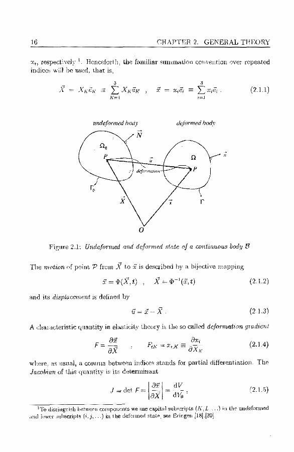
Consider a co11tinuousi defor1nable body B 1 of uniforn1 te111pera.ture; undcr the inftuence or an elastic defor111ation. A" point Pin the 'u.ndefo1·1ned state of body B: is characterized by its m.aterial or Lagrang1:an position vector X i \Vith respect to a fixcd origin 0, see Fig 2.1. In the deformed stat.e we denote the point P by it.s spat?:a.I. or Eu.leria.n position vect.or X1 again \Yith respect to 0. The coordinates of X. and i' witlr respect. toa Cart.esian basis {Oë1ë2ê;3} are clenotecl by X 1, and

16 CHAPTER 2. GEJ\'ERAL THEORY

~1:: 1 respectively 1 Hencefo1th, the fanüllar sn111n1flt,ion conventiou over repeated îndîces \viH be used~ that is,

3

L )<;(ëg }(""\

undeformed hody

N

deform((llóll

r, x

0

3

- I.::t:;e;. 1=.l

dcformed hody

r

(2.1.1)

n

Fignre 2 .1: Undcformed and defnrrned sta.te of a confrnuotts body 8

The rnMion of point P from X to :i' is described by a bijective mapping

x = if!(:R, t.) (21.2)

flnd its displacement is defined by

1.l=X X. (2.1.3)

A charncteristic qmmtity in ela.sticity theory is the so called dcfonnation gradicnt

F- ffi - a:R (2.1.4)

\Vhere; as usual: a co1un1a bet.,veen indices stn.nds for partial ciifferentiation. 1~he .Jacol.rian of t}üs quant.it..Y is its deternüBant

J = clct F = \aax:~ \ dV dV(,'

(2.L5)

distl11g11ish bet.,vceu con1poucnts \\'€ usc capita} suhscripLs (/~. L, .. ,) iu the undcfonned and luwer suhscriptf.l (1'.j, ... ) in th.; deforrnerl staie, see Eringen [18l.i20j.

2.J CONTINUU'vl MECBANICS 17

and is to be int.erpreted as the 1·at-io of t.he vohnne of a deforrned infinlte;:;irnal volu1ne ele1nent d\i and it.s undRforrned counterpart d\/0. Since t.he n1ass of snch an elen1r.-ut is t-o be conserved: i.e. d111 = 1xlll p0dl10 ::::;;; dmo) \Ye find the follo\\·ü1g rclar.ion b.et.\veen t.hr. defor1ned and undefor1ncd n1as.s deusît.y

Po= pJ ·

\>Ve furthe1 int.roduce the right Cauchy Green t.ensor C

1vhcre FT is t.hc tra.nspose of F: and the Lagrau,qc stra1>n. tensor E

1 E = -(C I)

2

(2.1.G)

(2.1.7)

(2.1.8)

Employiug the definit.ions (2.1.3), (2.1.4) and (2.Lï) in (2.1.8), we arrive at. the \veH-kno\vn expression for the co1nponent.s of t,he Lagrange straiu tensor

Eg1.

At any point .f of the defonned body Ll, 1.bc force acting on an inlinitesimal area ele1J1ei1t d.ii = ·i1.da., \Vith a Jlorn1al vect.or 'IÎ. = eau be \vrït ten a.s fda~ ,,·J1erc [ ls n. so caJ1ed simss ?H!r:.tor" J\ccording to a t1H~ore1u by Cauchy: the stress ,-eet.or {is lhlearl:"<~ dependent on 1.be nor1nal vector '1Î.

t = T iï t, {2.LlO)

\vhere tlte nun1bers T;j forn1 the con1ponent:s of the so called CfJuch.:1 stress tensor T. 1~he rctation bet\veeu the Cnuchy stress and the Lagra.nge strtÜn: is reflected in tl1e follo,ving const·it·utive cquatio"f1.

] &'E:. '!' T= F· -- · F

.J /JE l &E -1 F,I( "E . FJ1 . . . u l\ f,

(2.Lll)

\Yhere I: = I::(_Xg: E1\1 . ..J is tJ1e intêrnal eh1.stie energy. The genera! thcory of elastostatîcs in t.r.J1ns of the Canchy s1,resses: is fornn1-

lated wit.h respect to the, a priori, 11nk11ow11 deforrned region of the body Ll. In the 1.heory \VC are devcioping: ho,vcver: it. \vill be 1nore convcnicnt to have the eqnatlons forn1ulatcd 'vith respect. to t.he undeforrned configuratiou. To t.his end \\T; int,rodnce 1J1e seco11rl Piola J(irchhoff stressesTl\ï, (oT pseudo st-re':\Ses), by the following implicil delinition

(2.1.12)

18 CHAPTEn 2. GENERAL THEORY

From (2.l.11) and (2.1.12) we obtain the following material formulation of the constitutivc la\v,

à' T10, = àE~ .

f(L

The strcsses T1< L have the follo,ving propert.y

(2. l.1.3)

(2.l.14)

\Vhere d.4 = f\Ï-d.A is the unclefor1ned counterpart. of the area elen1ent dä. There­fore, the numbers F;1c T10, (the first PK stresses) are to be interpretecl as the

stresses at :ê, n1easured per unit area at X. The second PK-teusor T1\·L is the quant.ity of interest for the follo,ving sections on plate and shell theory.

2.1.2 Balance equations

The genera! thcory lor the elastostatics of solicls, wit.h respect to the undcformecl configura.tion) eau llO\V be sun1111arized as follo\vs

Problem 2.1 (E/a$f.ostatics, nwl.erial fornwlotion). Let the regfon \10 , occu7Jied

by the undefomied body B, have a. hounda"y r 0 = à\10 with v.nil norm al 1V. For givcn volume farces bi : flo --+ IF(, bounda'r7; t.ractions t/" : r Ot, --+ IR and baundary displacements 11;' : r0u, _,IR {where r·0", = r0 \ frn,, i = 1, 2, 3), find the mass density p1 displa.cements u1 1 strains E1..-i and stresses TKL = TLI<: su.ch that

j'' Po in f2o 1 (a)

(x;.K TKLJ._1, +Po b, 0 in D0 : (b) (2.1.15)

:c.;,f\· T1..:L 1Vt_ t' mi fot; (c) "

V,.I '/1.~ on.fo11;} (d) '

where the strains EKL are _qiven by (2.L9) and the stresses THL satisfy (2.1.13).

The equations in (2.1.15) have the following intcrpretation: (a) the balauce of mass, (b) the balancc of momentum, (c) clynamic boundary conditions and (d)

kinen1atical boundary conditions. The sets Do: r 0 and unit norn1a.l iJ in the undeforn1ed configuration: correspon<l \Vith the sets D: [ and unit nor111al 1î in the dcformecl configuration (sec Fig 2.1).

If \Ve are dealing \Vith the elastodyna1n.ics of solids) the second cquation in (2.1.15) must be changed into

(2.1.16)

and initia! con<litions, e.g. û(R, 0) = 170ancl u(R, 0) = 17o are needed in adclition, to obtain a well defined problem (here il is the material time clerivative of u).

2.2. RE!SSNEH-MINDLIN PLATE THEOHY 19

2.1.3 Constitutive equations

The theory present.cd here is not co111pletet:l: Ulltil specification of the înternal eliistic cnergy E. At this point, \VC assu1ne that the energy E has the follotving forn1

L = ~ E: 0: E = ~Diu,MN En1, E.11N (2.L17)

which, by virtne of (2.1.13). implies that t.hc stresses TgL depend in a linear wav on the st.rains E1a, tlrnt is

(2.118)

This formulation is still vcry generaL but only one cla% of mat.erial behaviour is of interest. here: i.e. orthotropic 111aterîa1. If \\'C iut.roduce the follo,ving abbreviat.ion:s for t.he stresses and the st.rains

u [Tn·. Tn·. 12:z, T.n·, T,z, '.fl'z)T {2.L 19)

f: [Exx· En·, Ezz, 2En·, 2Exz. 2Ei·zr.

equation (2.1.18) can be abbrcviated as

u=Df:, (2. 120)

where D is the nw.terial coefficient ma.tr'i:r.. For the e:\sc of linear orthotropic n1ateriaJ this syuunetrical n1atrix can be \tTitten as 3

D1111 Dun Drn:i 0 0 0 D2:122 D22:CJ:1 0 0 0

D D3:n.1 0 0 0 (2.1.21)

Di212 0 0 syrn1n. Dm3 0

D2.121

Notice th<tt although t.he const.itutive law is linear, the nonlinearities in the bal­ance equar.ions (2.1.15) are retained and thcrefore the theory is ealled geometri~ cally nonhnear. For a further introduct.ion to co11t.ïnuun1 111echa.nics the reader is referred to Eringen [18] aud [20].

2.2 Reissner-Mindlin plate theory

2.2.1 Introduction

In this se<:t,Ïon a grornetrically nonlinear plat.e t.heory is presented: v.:hich is hased on the Reissner-1\'Iindlin. assu1nptîons and is shnilar to the \vcll-kno\vn \!on J(ar-1na11n plate t.heory. The reasou to considcr a goon1etrically nonlinear theory here

isotroplc ca..:.;e is obl.ttined whcn D1122 D2233 = D1133, D,:H2 = D1;n3 = D2023 and D1111 D?.222 = D3333 = IJn22 + 2D1212

20 CHAPTER 2. GENERAL THEOHY

is t.hat. ta.pe defor111atio11s n1n;y becorne signiJicancly lnrger t.1'1an the tape thiek­ness. Fltrt:her1note! the R.eissncr Jvlindlin forn1ulation i:s chosen bec~1use it. alJo,vs for a finitc elen1ent. discretization by 1nea11,5 of c 0-eont.inuons tria.l solutions: to be desi::rihcd later In t his thesis,

The. line of teasoning follo,ved here is vcry silnilar Lo the 011e used by H ughcs in [39] (Chapt. 5 nml 6), bu1, n-it.h the main difforence tha1: our point of departure is the nonlin.eu.r 1naterial .fo·rrnula.tion of ela.•Itostatics as prescuted in (2.1.15 ). For a. rnore engine<::ring point. of vîe'v to plate t.lieor.'', the reader is rcferred to 1.ho:: well-kumrn book by Timoshcnko et al. [8ï] (especiaily Chapl. 2. 4, 12 amI B).

ln this SC:!ct.ion \Ve do not use the spatial (Euleriau) fonn11lat.iou: tliercfore \Ve

drop the cou,·cnt,ion of using 11pper casf~ indices (1-()_,;· .. ), Di.fl'erenf1.atio11s are o.lwa?H! vvit.h respect to the undcfor1ned positio11 and rnïly the seco·nd Piola /(irchho.ff sl:resscs are u8ed. ,i\.lso t.he subscript. o: as in Po: is ornit,ted, ln addltion: fron1 naw on, Latin indices (i, j) have t.he ralnes 1, 2, :J and Greek indicel (o, 11) have t.he v"1lue.s ] : 2 (also iu t.he s1u11n1.ation eonveution).

I_,e1. the region occupied hy aftar, plate: of thiekness d, be gi,·en h]"

ri {x= (.11,y,z) E IR" 1 (.1',)J) EG c IR' f\-d/2 s; z <: d/2} (2.2.1)

A subset of D with a fixed '"'lue of z is called a lariäna and a subset oI points wit.h fixed (.11, JI) = (x0 , y0 ) is called a fiber. The lamina at z = 0, is cal led (.he middle sm:face of the platc. The boun,fary of G is denot.cd by C: = fJG.

Reissner-Mindlin Assumptions

1. The plat.e is in a otat.e of 1ilan.e sl.ress, t!mt is 0.

2. A plate fiber: inïtîally straight r.111d perpeudicular r.o the 1niddle s11rface1

re1nains strn.ighf. but 1nay rotaLe about fl dîrcction in the tuî<ldle surfac0.

The se(;ond assun1pt.iou is a \\'Cakeniug of the fanliliar l(irchhoff--Love hypothesis: \Yhich st.ates t.hat fibers 111ust. al\vays re111aü1 perp('ndicul~u to t.he nliddle surface of t.he plate.

2.2.2 Displacement definitions

Any point: ·pof the undc)for1nt!d plat.c. haviug po.sitiou vect.or :f \vit.h respect toa fixcd basis {Oê1ë,ë'.1}, ean be writ.een as

i' = xo + f, (2.2.2)

'vhere :!!0 is a poü1t h1 l.he iniddle i:anface and f.... is tl vector î11 the fiber direction. Aft.er the dcforn1ation the point P l1aE 1novcd fro111 :C to fl: \Vherc

(2.2.3)

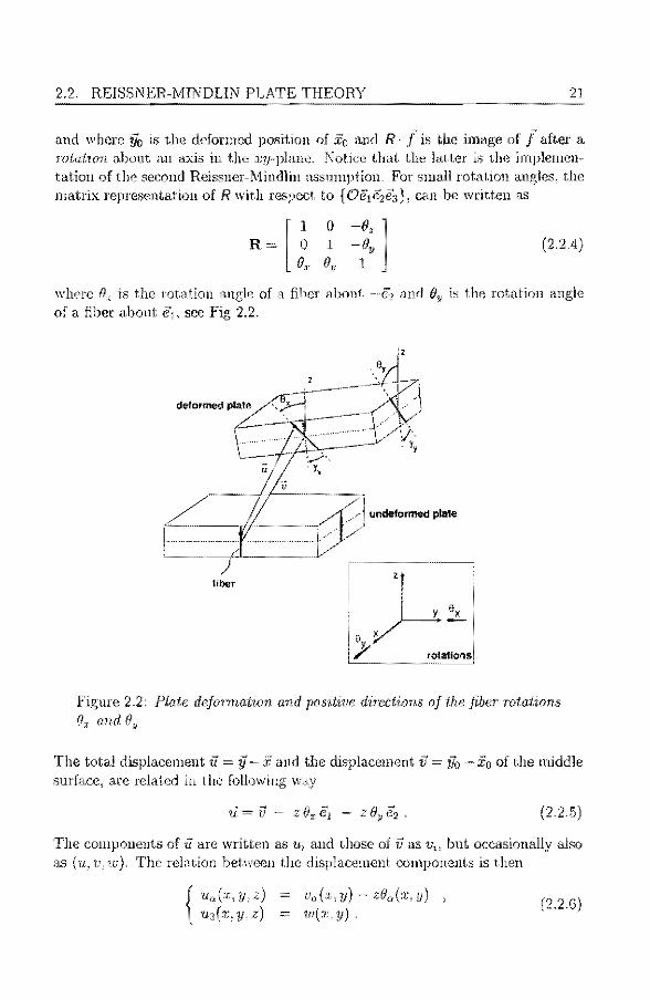
2.2. REISSNER-MINDLIN PLATE THEORY 21 ~~~~~~~~~~~~~~~~~~

and wbere fio is the cleformcd posit.ion of x0 Md R · fis the image of F ah.era 1"0tation ahout an ax.is in the .i:y-plane. Notice that. the latter is the in1plen1en­tation of the second Reissner-h1indlin ass1n11ption. For s1nall rot.ation angles: the n1atrix represent,atlon of R \Vit.h respect to {C?ë1ê2e'.:i}: ca-n he \VTÎt.tcn as

R=[~ 0,"

0 -B,. ] 1 -o.

&, 1 (2.2.4)

\\'here Oz is the rotation angle of a fiber about of a fiber abollt €:, see Fig 2.2.

and By is the rotatïon angie

undeformed plate

1iber

Figure 2.2: Pia.te defonnation and posi.twe directions of the fiber roi.ations IJ, and O,

The total di.splacement 1Ï = y - i! and die displacement ïi = 170 - in of t.lw middle surfru:e, are related in the following way

Û= fJ - zOx~ (2.2.5)

The co111µone11ts of ·il are \vrit.ten as 11.1 and those of i: as Vi! bnt occasionally also as (u, v, w ). The relation bet.ween t.he displacemcnt compouent.s is then

v0 (x, y) - z00 (:c, y) 111(>:, y) . (2.2.6)

22 CHAPTER 2. GENERAL THEORY

2.2.3 Constitutive equations

The ür1plenH:!ntation of the first R,eissner-1vlîn<llin Ftssun1ptîon: Le, the plaue streS3 couditiou Tzt = 0, has consequenees for the for1n of Lhe constitutive equ.a.tloIJs as presented in (2.1.19) to (2.1.21). The usual way to modif.l these <e'<juaüons is LO

eliniinate E~z, yieldiug the follo\vÎug expre~sslons

Dll3:l E + D,,.,,, E ) (2.2.7) D:,3:-13 XX D:f-1:13 lj!) :

111 the general ort.ltot,ropic case, llcdcfining the stress vector O' and .strain vector e of (2.1.19} as

IY ITn, 'Tit!J! 'T:i:y, T~Zl T,Jr

g [E,x. EYY• 2E.,._y: 2E," 2E,,] T

the constitutive equation can agait1 be \\:ritten as

(2.2.9)

The material coefficient mat.rix D for t.he oühot.ropic case is now writ.ten in the follO\Ving \VCH-kuO\Vll for1n

E, vyEx 0 0 0

lixll.y 1 - l.!,-r:l/y

r.1xEY"" E y 0 0 0

D 1 /.IJ)/y l ~--· l.lxlJy (2.2.10) 0 0 G,y 0 0 0 0 0 Gxz 0 0 0 0 0 G,,

\vhere Ex nnd Ey are t.he ":{oung rnoduli in .L a,nd y direction and lfx and ziy the corresponding Pois.son ratios. 1'he shear n1odulï a.re related by Gxz = G11 ::: = "'·Gxy, \Vhere the nnrnber Kis called t:hc shear correction fr1cto1·. Strictl,y speakîng \VC have 1<. = 1, but in the Reissner-Mindlin theory it is het.ter to t.ake i;; = 5/G, because this choice yields better results with respecl. to classica! bendiug theory. For a derh."at,îon of this fact.or and generalîzations: see Tünoshenko {86]. A conunon choice for Gxy is the fo11o\viug haTtnonîc 1ncan value of shcar n1oduJi in 1: a.ud y direct.ion

1 = l1l+vx-'- J+i;,) Ex ' Ey G'xy

Because of t.he synnnet.ry of D

(2.2. ll)

we have in addit.ion the followiug rela.tionship

Vx Ey = l/y E, . (2.2.12)

Obviorrsly, t.he isotropic case is ob1.aü1ed if these codlicients satisfy E,, = Ey and Vr:. = uy. For rnore infor111ation on anisotropy of plates an<l shells: see the hook by Lekhuitskii [59], Section 2.

2.2. REISSNER-MINDLIN PLATE THEORY 23

2.2.4 Strain-displacement equations

Aft.er the formulation of the precise cxprcssions for the displacement.s iu (2.2.6), it is easy to obta.i11 expressio11s for the Lagrange strains Er1 of (2.1.9). An ünportant. step: hü\\-"ever! in the derivat.ion of a f5in1ple geo111ctrically nonlînear plate theory: is t.o delete scveral t.cnns in t.he nonlinear part. of equat.ion (2.1.9). To this end \re split this nonlinear tern1 in the follo\ving \Vay 4

(2.2.13)

The second term in t.he right. ha.nd sidc of (2.2.13} is now omiLtcd. because defor-1nations due to in-plane displa.ce1neut.s are a.ssn1ned to he s111alL Using the fact. that u3 = u:(J: 1 y )~ \\'e caD \\Titc the sünplifierl st.rains in the for111

(2.2.14)

Remark. The stJ·ain E=, is left, out of considerntiou for tbc reason mentioned in the prevlons suhsection. Notice. ho\\:everr t,hat calcnlation of t.his str;Ün fron1 (2.2.14) gives = 0 and t.his is in coutradictiou wit,h the prcviousl,v found expressious in (2.2.ï). Tltis is a \vell-kno\Yn inconsîstency in plate theory1 \vhich ïs U$ually accept.e<l because the theory gives good resnlt.s.

Upon subst.itution of all displacement. components of (2.2.6), e41iation (2.2.14) becon1es

q• ' -1- ! 11' 'L' n "(o,8; • Z fJJ.''.tJ ~ 2fl(u.D) .-(2 2.15)

1.D.0 - Bo

The new sombols introduced in (2.2.15) have the following interpretation, euB

are the 1ne1nbranl': stmins1 ",..·of:J are c1L11;atures and "'la a,r·l~ shr:or st.1nins. The 'Yo are 1.he rot.ations of a fiber. wit.h respect. t.o 1.he nomrnl on the defonnecl middle surface_, \vhe1cns the -u;. 0 a,re r,he slopes of the plate.

Re111arks. 1. j\Tot.ice that. in general t.he fiber rotncion ()0 diHCrs fro111 the siope 'W,o· In the U1in platc limit, i.e. d L 0, this differente will vanish. 2. A condit.ion undcr "·hid1 (2.2.15) is \'alid is that w,0 w~ must be comparnble to V{c..8)·

3. The rotat.ion abont the nonna! of the plate, somctimes callecl a dn/linq dcgree of Jreedom (sec Hughes and Brezzi [401), is not considercd beca.nse plat.es rmct usua.ll.v n1uch stiffer against this kind of defor111ation.

het.ween pan:-nthescs deuotc the syrru11el.nr.of part of a tcn~or, 1vhcreas sohscripts in square hrackcts denoLe it..s (ltJtl-syrnmet.ricrJ parL: iJ1a1 is u (>.;/ = fr{'1t1. i + 11j, t) a11d 1.t [i.jj = ~(11.i,:J Vj. 1).

24 CHAPTER 2. GE>lERAL THEORY

2.2.5 Balance equations

Aft.er sitnpllficat.ïou of the strain-displacernent relat,iou~! the balance e<3uacions can be t,reated in a simîlax \va.y. \·\1e \\Tlte the st.ress eqniHbriurn equation (b) of (2. l 15) expre.ssed in terrns of the displace1nent gTadie11lB

(2.2. 16)

where pb; has been rcplaced by j,. The second, nonlinear term in (2.2.16) is now treat.ed i11 the sarne way as was done in (2.2.13): for i = o = L 2 this t.erm is 0111itted, \vherea.s for i = 3 it is retained, yieldîng

.,.. In = o, (2.2.17)

The san1e sin1plification îs a.pplied to t.he stress boundary conditions

1~j Tij

T33 ·nj + 'IJJ. k 'L-i 11.j = (2.2.18)

The final step towards a plate thcory, is the int.egration of the simplified bahmce equations and boundary coHclitions in the t.hickness direct.ion of the plate. As rui exan1ple, \Ve den1onst,rale r.his procedure for the in-plane stress equilibrïu1n . . !\ con1plct.e s11111n1a:ry of not.H.tion conventions and equatîons ïs given iu the next. suhsection. Consider the first equation in (2.2.17) and perform int.egrntion in the z-direction

l d/2 (d/2 ( T;,;"1 + J0 ) dz = .. ( T0 5"; + T0 :u + fu ) dz =

-dj'l .. -d/2

( !d/? T0 a dz) + (t~) + jd12

f 0 dz = 0 , (2 2 19) , -d/2 . fJ -d/2

(2.2.20)

into (2.2.19), we finally arrive at t.he in-plaue equilibrium equa.t.ions

(2.2.21)

2.2. REISSNER-MINDLIN PLATE THEORY 25

2.2.6 Summary of plate notations and equations

Vo: (or: 1t, v) in-plane displacements

w deflection

Oo: fiber rotations

eo:p V(o:,p) + ~W,o:W,p membrane strains

""op O(a,p) curvatures

"fa W,a - Oa shear strains

di2 Nap = j 1

Tas dz membrane forces per unit length -d/2 '

f d/2 Map z Taµ dz bending moments per unit length

' -d/2

Jd/2 Qo: = Ta3 dz transverse shear forces per unit length

-d/2

Jd/2 fa dz +

-d/2 (t~} resultant applied in-plane forces

d/2 Ga

fd/2z dz + (zt~) resultant applied couples

Jd/2 p · f3dz + (t;3) effective pressure load

-d/2

Jd/2 N<: dz boundary forces per unit length

-d/2

M* a Jd/2

-d/2 zt~ dz boundary moments per unit length

Q Jd/2 t3 dz boundary shear force per unit length -d/2

Q* = w,aN~ effective boundary shear force

Dt Ed

tensile stiffness (isotropic case) = (1 v2)

Db Ed 3

bending stiffness (isotropîc case) 12 (1 v2)

Ds r;,Gd shear stiffness (isotropic case)

nt afl"f/5 ' D~/318' D~P tensile, bending and shear

stiffnesses ( orthotropic case)

26 CHAPTER 2. GENERAL THEORY

Figure 2.3: Sign conventions for membrane stresses, bending moments and transverse shear forces

Problem 2.2 {Reissner Mindlin Plate). Let the region G C JR2 , occupied by a flat plate, have a boundary C = 8G with unit norrnal n. For given plate loads Fo., Ga and p, boundary loads N~, M~, and Q*, boundary displacements v~, w* and rotations B~, find displacements Va, w and rotations Ba such that

0 in G,

0 in G,

0 in G.

The conditions to be satisfied on the boundary of the plate are

(2.2.22)

{

Va on Cva ' Naf3nf3 N~ on Cn"' = C\ Cva' w = w* on Cw , Qa na = Q* on Cq = C \ Cw , (2.2.23) Ba B~ on Gea , Maf) n11 Af~ on Cma = C \ Co0 ,

where the membrane stresses Naf3, the bending moments 1vlaf3 and the shear forces Qo. satisfy the following constitutive equations, in the isotropic case,

{

IVafJ =

1\1a:f3

Qa Ds/a,

Dt[ (1 - V) ea,a + V ÓafJ e'Y,] , - Db [ ( 1 v) K,<>fJ + v Óaa K,'Y'Y] , (2.2.24)

or in the more general orthotropic case

Nafl D~,a,óe'Yó , Mnf3 = -D~fJ'Y8K'ró , Qa = D~fJ/,6. (2.2.25)

2.3 A simple nonlinear shell theory

2.3.1 Introduction

In this section the nonlinear plate theory from Section 2.2 is generalized for the case of curved shells. This generalization is not as rigorous a'> possible, but

2.3. A SIMPLE NONLINEAR SHELL THEORY 27

su:fficient for the problems under consideration. A very concise overview of the "exact" nonlinear thin shell equations, based on a modification of the Kirchhoff­Love hypotheses, is given in the well-known paper by Koiter [47]. A nice overview of several simplifications that can be derived from the exact theory, is by Sanders in [77], whereas a very complete picture of the general theory can be found in the monograph of Niordson [69]. In all these references the shear strain is not taken into account.

The theory presented here is very similar to the Donnell-Mushtari- Vlasov (DMV) theory (see Niordson [69], Chapter 15), hut based on the Reis.mer Mindlin assumptions so that it can be used in a finite element model with c0 continuous trial functions. The DMV formulation, originally designed for the study of buck­ling phenomena in plates and curved shells due to in-plane loads, is one of the simplest geometrically nonlinear shell theories suitable for the present application.

To understand the equations of this model, the reader must have knowledge of tensor analysis in curvilinear coordinate systems. Therefore, we have included some results of this mathematica! tool in appendix B. The reader not familiar with tensor analysis is urged to read this, before continuing. Moreover, definitions and symbols not declared here can be found in the appendix.

2.3.2 Fundamentals

Let a point x in a curved shell, of thickness d be defined by means of its normal coordinates Ç1' e, ç3 (compare with (2.2.2))

1(ç1, e, ç3) = r(e, ç2) + ç3rr(e1, ç2), (2.3.1)

where f(Ç°') is the position vector to a point in the middle surface and n is the unit normal on the middle surface at f. The space occupied by the shell is the following set

(2.3.2)

A subset of 0 with Ç3 = constant is called a lamina of the shell, whereas a subset of 0 with a fixed value of ( Ç1, ç2 ) is called a fiber. The special lamina for which ç3 0, is called the middle surface of the shell and is denoted by S. The boundarv as of s has a unit normal it. that is perpendicular to the normal n of the middle surface, i.e. ii = fi<> a(X ' where aa = f'," are tangent vectors to the middle surface. The region G has a boundary C 8G, so that formally we can write as = f( c ).

The displacement of an arbitrary point in the shell, can again be decomposed into a displacement of its footprint in the middle surface and a rotation of the corresponding fiber (compare with (2.2.5))

ü = v E,3B1a1 - ç3 (J2a2 = ( v" - ç3 ()<>) aa + wii. (2.3.3) '-..,.-'

u"

28 CHAPTER 2. GENERALTHEORY

A better motivation for this displacement field is given in Appendix B, together with a short derivation of the following strain-displacement relations for the shell

Eaf3 eaf3 - ç3 Kafj 2Ea3 "' ra)

ear; = V(ajB) ba.BW + a·w,,a' (2.3.4) Ka/3 tl(alB),

~fa ·w,a - Ba .

In (2.3.4) the symbol 1 stands for covariant differentiation with respect to the coordinates ça, whereas ba{3 is the curvature tensor of the middle

The equation for the membrane strains eaf3 is the same as in Niordson [69], Section 15.3. Compared with the equation for eaf3 in a more rigorous nonlinear theory (see Niordson [69], Section 3.3), it can be shown that the nonlinear terms in containing expressions of the form Ua 1 {3 and b~ u,s, or combinations of these, are consistently ignored.

Stress resultants are defined in the same way as for the plate

( ' QQ) l d/2 ( ya{3 ' e yaf3 ) yo.3 ) dç3 . -d/2

(2.3.5)

It must be noted, that for curved shells this is only an approximation for the stress resultants. In the more rigorous formulation of shell theory, higher order terms in , containing factors b0 p, are also present in the integral on the right-hand side of (2.3.5), (see Niordson [69], Section 6.4). An approximate distribution of the stresses Tii, that is at most linear in ç3 is given by 5

+ 733 = 0. (2.3.6)

When using these approximations, errors of the order d/ R and ( d/ L )2, where R is the smallest principal radius curvature and L is a characteristic length of the shell, are generally accepted.

2.3.3 Shell equations

With the above definitions .the DMV-equations hased on the Reissner Mindlin hypotheses become

Problem 2.3 (Nonlinear Reissner Mindlin Shell). Let a set G C JR2 of surface coordinales deterrnine the middle surface S of a shell. The boundary aS of S,

5If the shear stresses Ta3 are

3requir[ed to (v~n;~h) ;tJ

these stresses would be T"3 = 2

d 1 d ·

d/2, a better approximation for

2.3. A SIMPLE NONLINEAR SHELL THEORY 29

corresponding with the boundary C of G, has an in-plane unit norrnal n. For given shell loads po., co. and p, boundary loads No.*, Mo.*, and Q*, boundary displacements v~, w* and rotations (}~, find shell displacements Va, w and fiber rotations (Jo. such that

0 in G,

0 in G,

0 in G.

The conditions to be satisfied on the boundary of the shell are

No.* on Cn"' = C \ Cv"' ,

(2.3.7)

w = w* on Cw , {

Va = V~ on Cva ,

Q* on Cq = C \ Cw , (2.3.8)

(Jo. (}~ on Ge"' Ma* on Cm"' = C \ Ge"' ,

where the membrane stress es No./3, the bending moments Mo.J3 and the shear farces Qo. satisfy the following constitutive equations (in the isotropic case)

{

No./3 = Dt[(l -v)eo./3 + vao.f3e~], Mo.J3 = -Db[(l-v)h:o.J3 + va°'f3h:~], Qo. = Ds ry"''

with a similar extension to the orthotropic case like in (2.2.25).

(2.3.9)

Here, a"'/3 are the contravariant components of the metric tensor of the middle surface. Besides the use of covariant differentiation, the salient difference between the shell equations above and the plate equations, is the presence of the curvature tensor b<>/3 in the expression for the membrane strains e<>/3 as well as in the out­plane equilibrium equation. The latter implies that in a situation where (Jo. and w are identically zero, membrane stresses N"'/3 can only occur in the presence of a load carrying pressure p.

Example (Cases of bending and stretching relevant in magnetic recording). • Consider the case in which a flat plate is bend into a cylindrical panel of radius R. Assume that eo./3 = 'In = 0 and that the only nonzero curvature is given by h:xx = -1/ R. From the constitutive relations (2.2.24), we conclude that the bending moments needed to obtain the cylindrical shape of the plate are

M _ vDb YY - R Mxy = 0.

• Conversely, assume that Mxx = M is the only nontrivial bending moment (all other stresses remain zero), then (2.2.24) implies that

-M vM h:xx = Db (l - v2 ) ' h:yy = Db (l - v2 )

h:xy 0.

30 CHAPTER 2. GENERALTHEORY

In other words, the plate becomes a doubly curved surface with two oppositely signed curvatures. This is called anticlastic bending. • Consider the shell equations (2.3.7) for the case of a cylinder of radius R, for which w B°' 0 and Nxx = Nxx T is the only nontrivial membrane stress. The out-plane equilibrium can only be satisfied if we apply a load (see example 1 in Appendix B)

p=

which is called the hoop pressure.

2 .4 Reynolds equation

In this section we formulate the equations, which describe the phenomenon of lubrication that was shown to be of importance in Section 1.2 on the helical scanner. For a rigorous introduction into this subject, we refer to the works of Gross (35] or Walowit and Anno [90]. Both hooks contain a chapter on foil bearings. A derivation of lubrication theory within a somewhat more general context is given by Tanner in [84], Chapt. 6.

Lubrication is a phenomenon where a fluid (lubricant) flows within a thin film, the narrow gap between two surfaces. Let us denote this film, for all t ~ 0, by

0 = { (x, y, E JR3 1 (x, y) E G C JR2 0 :S z :S h(x,y,t)} . (2.4.1)

two subsets of 0 at z = 0 and z h are called bearing surfaces, and the quantity h(x, y, t) is called the film thickness (sec Fig 2.4). The boundary of G is denoted by C &G. The lower hearing surface is assumed to be flat, although this is not essential. The lubricant is considered here as a compressible,

Figure 2.4: Lubricating film between bearing surfaces

2.4. REYNOLDS EQUATION 31

instationary, Stokesian fluid 6 , of uniform temperature and viscosity. There are five fundamental unknowns, which describe the state of this fluid

p, p, vi (i 1,2,3), (2.4.2)

where p is the mass density, p the press·ure and vi (or : u, v, w) are the velocity components of the fluid. All unknowns are functions of the spatial position i and timet.

The prescribed velocities of the fluid at the upper and lower surface, are written as vi(x, y, 0, t) Uf (x, y, t) and vi(x, y, h, t) = UNx, y, t), respectively. The sum of these hearing velocities is also of importance and denoted by Ua := U2 + U~, where a L 2 (in addition we take U~ = 0).

By employing certain thin film approximations, we can simplify the equations of fluid dynamics considerably to the so called lubrication equations. A precise derivation can be found in Appendix C. The resulting lubrication problem, in­cluding boundary conditions and initial conditions, can be summarized as follows.

Problem 2.4 (Lubrication Problem, compressible case). Let G C IR2 be a lu­bricated region, having a boundary C 8G with unit normal n, and [O, T] c IR a time interval. For a given film thickness h : G x [ü, T] --+ IR, bearing ve­locities U°' : G x [O, T] --+ a lubricant viscosity 71, a boundary pressure p* : CP x [O, T] --+ IR, a boundary flow q* : Cq x [O, T] --+ IR, (where Cq C \ Cp) and an initial pressure Po : G --+ IR, find the lubricant pressure p such that

(ph3P,a ),a 677 (phU a ),a oph

in G x [ü, T], + 1277-ät

p p* on Cp x [ü, T], (2.4.3)

Qana q* on Cq x [ü,T],

p Po at t = 0, in G,

where the lubricant flow qa per unit length is given by (see also (C.11))

(2.4.4)

The density p and the pressure p are related by the gas law (C.3-e). The first equation in (2.4.3) is the well-known Reynolds equation for the compressible case. Once the pressure is known the lubricant velocities follow from

Uo) z 1 +­°' h 2.,, z - h) P,a. (2.4.5)

6A Stokesian fluid is a Newtonian fluid, in which the shear viscosity T/ does not depend on the mass density p and the bulk viscosity is zero

32 CHAPTER 2. GENERAL THEORY

For an incompressible lubricant the density p remains constant and can be elim­inated from (C.13). Thus, the Reynolds equation for the incompressible case is

äh 6r1 ( hU a ),a + 1217 ät . (2.4.6)

For very narrow hearing gaps, the film thickness may become comparable to the molecular mean free path in the lubricant. In this case slip may occur at the hearing surfaces. Consequently, the Reynolds equation must be modified in order to take account of this phenomenon, see for instance Mitsuya [64]. The Reynolds equation for the case of slip flow is given by

(2.4.7)

where Àa is the ambient molecular free path length and Pa is the ambient pressure. The so called Knudsen number Kn = Àa/ H, where H is a characteristic film thickness, is the indicator for the occurrence of slip flow. If K n < 0.01 use (2.4.3) and if 0.01 < Kn < 1 use (2.4.7). If the film thickness becomes too small, even a higher order approximation of the slip flow effects may be necessary (Mitsuya [64]).

Remarks 1. Until now the hearing surfaces were assumed to be rigid. As may be clear from the previous chapter, one of these surfaces is formed by the magnetic tape and is thus very flexible. Moreover, the lubricant under consideration is air. This is where the concept of the foil bearing comes into the picture. The film thickness h is related to the deflection of the plate and the air pressure acts as a load on the tape. Since the presence of the film thickness in the Reynolds equation is cubic, we see that the coupled plate/lubrication problem is strongly nonlinear! 2. The Reynolds equation above, has been derived in a Cartesian coordinate system. If the lubricant flows between two (not too strongly) curved surfaces, it is not difficult to show (see also the theory in Appendix B) that the generalized form of equation (2.4.3) is

(2.4.8)

where 1 stands again for covariant differentiation with respect to a pair of surface coordinates Ç°'. 3. In Chapter 3 we will use the incompressible equation (2.4.6) for the ID foil bearing problem, although this restriction to incompressibility is not strictly nec­essary. more general Reynolds equation ( 2.4. 7) will be used in the rigorous 2D case in Chapter 4. In magnetic recording, compressibility and slip flow are for instance relevant on tape streamer heads, where the film thickness is only a few times the molecular free path length. But of course also in a near tape contact situation on a scanner with rotating heads.

33

Chapter 3

The one-dimensional foil hearing

3.1 Introduction

In the previous chapters it was explained that magnetic tape is lubricated due to the presence of a thin layer of air between tape and scanner. In this chapter this phenomenon is investigated more thoroughly, using the theory of Chapter 2. Before presenting the numerical treatment of the full two-dimensional problem, it has certain advantages to start with the simpler one-dimensional case. Firstly, because many of the difficulties representative for the foil bearing problem are already present in the lD case, whereas it is easier to show the nature of the difficulties and develop a strategy to solve them. Moreover, a one-dimensional approach leads to finite element models with a relatively small number of degrees of freedorn, and thus modest computation times.

Although the lD case has been treated in many papers on foil bearings, as was indicated in the literature survey of Chapter 1, the way in which the model is presented here still contains several unique aspects. Anyway, the numerical solution of the lD model will shed enough light on the problern, so that we will be better prepared for the rigorous 2D case.

In Section 3.2 the lD foil hearing problem is generally described and the formulation of a mathematical model for it is given in Section 3.3, where we couple a non-linear version of the Timoshenko beam equations to a special lD version of the Reynolds equation, to account for side leakage of air at the lateral tape edges. Typical problems to be dealt with are the strong nonlinearity of the equations and instationary effects.

The weak forrnulation, time discretization and linearization of this model are given in Sections 3.4-3.5, whereas the specific finite element formulation is given in Section 3.6. Care has to be taken to avoid well-known locking phenornena occurring in the case of thin tapes. Basically, the derivation that leads to the lD FEM model will be the same for the 2D case in the next chapter. \Ve conclude with sorne typical numerical examples in Section 3. 7.

34 CHAPTER 3. THE ONE-DIMENSIONAL FOIL BEARING

3.2 Problem specification

Consider a piece of tape, with length f,, width b and thickness d, wrapped around a rigid drum of radius Rd Fig 3.1 ). Elastic constants of the isotropic tape are its Young modulus E and Poisson ratio v. The length of the wrapped region is denoted by a aRd, where a is the angle of wrap. The drum is completely rotating with a circumferential velocity U 21rwRcz, where w is the number of drum rotations per time unit. A fixed lower drum and the helix angle, are not considered here.

A uniform tape tension T is applied at the beginning and end of the tape, so that the total applied tensile force is given by Ft = Tb. This implies that no friction between tape and drum is taken into account.

Next, consider tangent lines to the drum, at the beginning and end of the wrapped area. A longitudinal coordinate x runs along these tangents and over

(inlet) (outlet) (a)

T T

' : L. ' ' ' ~---- ... --- ~---~----------' '

T (b)

' ' ' ' T '

Figure 3.1: Geornetry of a foil bearing consisting of a tape wrapped around a cornpletely rotating drum: { a) lateral view, (b) unf olded tape path

3.3. ONE-DIMENSIONAL MODEL 35

the drum through the wrapped region, where we put x = 0 in the middle of the wrapped region. The transverse coordinate y is perpendicular to x and parallel to the drum axis. We call the region where x < -a/2 the inlet region and where x > a/2 the outlet region.

The tape defiection w and the position of the drum surface hd are measured with respect to these coordinates. Because of the drum rotation an air film of thickness h is present and described by (see Fig 3.1)

h = ha+ w,

where the drum geometry hd is approximately given by

{ ( lxl a/2 )2 , if

ha = 2Ra 0 l if

lxl > a/2,

lxl :s; a/2 .

(3.2.1)

(3.2.2)

The transportation speed Ut of the tape is much smaller than the rotation speed U of the drum and is therefore neglected in the analysis. The ambient value of the pressure pis denoted by Pa. The main quantities of interest in this model are the film thickness h and the film pressure p. In the following sections it is explained how to calculate these quantities.

3.3 One-dimensional model

3.3.1 Elastic equations

We start with the formulation of the lD equations describing the elastic equi­librium of the tape, using the theory of the previous chapter. More specifically, the equations (2.3.4), (2.3.7) and (2.3.9) for the case of a cylindrical surface of radius R are used. In example 1 of appendix B, it is shown that the metric and curvature tensor in this case are

_!:_ [-1 OJ R 0 0 . (3.3.1)

Since a013 is the unit tensor, there is no need to distinguish between covariant and contravariant components of a tensor. And because all Christoffel symbols vanish, covariant and partial differentiation are identical ( see appendix B). To be able to use the coordinate system ( x, y ), introduced in the previous subsection, the radius R in (3.3.1) is made dependent on x as follows

R = R(x) = 00

' {

if

Ra , if

lxl > a/2,

lxl :s; a/2. (3.3.2)

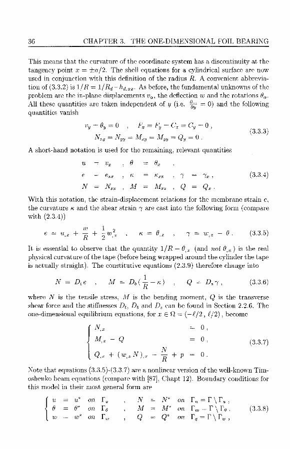
36 CHAPTER 3. THE ONE-DIMENSIONAL FOIL BEARING

This means that the curvature of the coordinate system has a discontinuity at the tangency point x ±a/2. The shell equations fora cylindrical surface are now used in conjunction with this definition of the radius R. A convenient abbrevia­tion of ( 3.3.2) is 1 / R = 1 / Rd - hd, xx. As before, the fundamental unknowns of the problem are the in-plane displacements Va, the deflection W and the rotations {)°'. All these quantities are taken independent of y (i.e. = 0) and the following quantities vanish

Nxy = Nyy = j\;fxy = i11yy Qy = 0 .

A short-hand notation is used for the remaining, relevant quantities

u

e

N

()

r Q

rx)

(3.3.3)

(3.3.4)

With this notation, the strain-displacement relations for the membrane strain e, the curvature ;;, and the shear strain ~f are cast into the following form ( compare with (2.3.4))

w 1 e = U,x + + w

2

R 2 ,x K = O,x 'Y = W,x () . (3.3.5)

lt is essential to observe that the quantity 1/ R - O,x (and not e, ) is the real physical curvature of the tape (before being wrapped around the cylinder the tape is actually straight). The constitutive equations (2.3.9) therefore change into

N 1

lvf = Db ( R - ;;, ) (3.3.6)

where N is the tensile stress, 11;[ is the bending moment, Q is the transverse shear force and the stiffnesses Dt, Db and Ds can be found in Section 2.2.6. The one-dimensional equilibrium equations, for x E fl (-€/2, €/2), become

r· 0,

M,x - Q 0, (3.3.7)

Q,x + ( W,x N ),x N

0. R

+p

Note that equations (3.3.5 )-( 3.3. 7) are a nonlinear version of the well-known Tim­oshenko beam equations (compare with [87], Chapt 12). Boundary conditions for this model in their most general form are

{~ u* (ffl

()* on w* on

r11. fe fw

N M Q

N* on r n r \ r u ,

M* on r m = r \ fe , Q* on r q = r \ r w )

(3.3.8)

3.3. ONE-DIMENSIONAL MODEL

where r = {-P/2, P/2}. In the case of the foil hearing a logical choice is

u(-P/2)

N(+P/2)

0

T

w(±P/2) = O

M(±i/2) O

37

(3.3.9)

hut there are other possibilities. The memhrane stress N could be eliminated from equation set (3.3.7) because the first equation N,x 0 implies that N must remain constant, i.e. N T. In the thin plate limit, i.e. 0 ~ w,x , the only remaining equation would then be

1 D" h,xxxx + T ( Rd - h,xx) p, (3.3.10)

where the physical tape curvature can be >vritten as 1/ Rd - h,xx· Equation (3.3.10) corresponds to the one given by Eshel and Elrod in [26]. However, the first equation in ( 3.3. 7) is kept as it is because of generality. Finally, it is remarked that the case of elastodynarnics can be treated by changing the third equation of (3.3. 7) into

Q,x + (w,xN),x (3.3.11)

where Pd = Pt d and Pt is the rnass density of the tape per unit volume.

3.3.2 A veraging the Reynolds equation

To arrive at a one-dirnensional model for the Reynolds equation, the second di­rnension is not just simply eliminated, as W&'> done for the elasticity equations. Instead, the Reynolds equation (2.4.6) is averaged over the width of the tape in the same way as done by Fijnvandraat in [29]. To this end, the mean value < rp > for an arbitrary function rp = rp( x , y) is defined by

< rp > 1 /b/2 b -b/2

x, y) dy.

The pressure p is still dependent on y and written as

p( x , y ) = Pa + p( x) f (y) ,

where f(y) is chosen in such a way that

b/2) = 0 <!>= 1.

(3.3.12)

(3.3.13)

(3.3.14)

Because of the first condition the pressure automatically satisfies the boundary condition p = Pa for y = ± b/2. Consider the incompressible Reynolds equation (2.4.6) with Ux = U constant and Uy 0. Applying the averaging operator (3.3.12) and using h h(x), together with (3.3.13) and (3.3.14) gives

(3.3.15)

38 CHAPTER 3. THE ONE-DIMENSIONAL FOIL BEARING

where c := [f'(b/2) - f'(-b/2)]/b. The second term in (3.3.15) is a first order approximation for the side leakage of air, due to the finite width of the tape. The number c is called here the leak factor. A ver age flows can be determined by applying (3.3.12) to the flow definition in (2.4.4) (take p = 1)

< qx > = -h3

1217

A reasonable choice for f (y) is

n+ 1 ( -- 1 n

f(y)

hU +2, < qy > 0.

(n > 1).

(3.3.16)

(3.3.17)

The case n = 2 is treated by Fijnvandraat in [29]. Allaire and Benson, in their paper [3] on rigid slider bearings of finite width, consider a similar function as in (3.3.17) and show that there exists an optimal value n i 2. Notice, that although the average flow in transverse direction vanishes, because of symmetry, the flow at the lateral tape edge (y ±b/2) equals 2(n + l)h3p / 1217 b. After some calculation the leak factor c for the present case becomes

c (3.3.18)

The correct coupling between the averaged Reynolds equation (3.3.15) and the elasticity equations is obtained if the symbol p in ( 3.3. 7) is replaced by p (the ambient pressure causes no tape deflection). To keep the notation simple the tilde in p is omitted in the subsequent analysis.

3.3.3 Complete set of equations

Problem 3.1 (Instationary 1D Foil Bearing). Let n (-t/2, R/2) c IR have a boundary r = {-t/2, i/2} and let [O, te) c IR be a time interval. For given numbers e, a, c, Rd, U, 11, b, d, E, v, and functions R, hd and Wo, find the relative pressure p, the displacement u, the defiection w, the rotation e and the film thickness h such that in n x (0, te)

( h

3 P,x) + ch3

p

1217 ,x 1217 N ,x

Q

Q,x + (w,xN),x

h

N R + P

u 2

h,x + h,t

0

0

0

The initial condition to be satisfied is

w(x, 0) wo.

(a) '

(b) '

( c) ' (3.3.19)

(d) '

( e) .

(3.3.20)

3.4. WEAK FORMULATION 39

The strains e, "'' 'Y and stresses N, lvl, Q are given by (3.3.5) and (3.3.6), re­spectively. The general boundary conditions are

r = 0 on r,

~ = u* on ru N N* on rn,

(3.3.21) ()* on fo M Jlif* on rm' w* on f w Q Q* on rq.

3.4 Weak formulation

The weak formulation of problem 3.1 is derived in this section. For the basic concepts and notations used here, the reader is referred to the well-known book by Hughes [39]. We start by introducing the following function spaces

Lz(O) = { u : 0 ___, IR

H 1(0) { u E L2(0)

k lu(x)l2 dx < oo } ,

du dx E L2(n)}.

(3.4.1)

Here L2(0) is the space of square-integrable functions and H 1(0) is the first order Sobolev space. To find a solution to the problem in a weak sense, trial solutions are taken from the following sets, at every time t E [ü, te]

P = { p(., t) H 1(0)

u { u(., t) E H 1(0)

W = { w(., t) E H 1(0)

8 { 0(., t) E H 1(0)

p 0

u = u*

w =w*

B B*

on r}'

on ru}' (3.4.2)

on r w}'

on fo}.

Weight functions are not depending on the time t and satisfy the homogeneous essential boundary conditions. The corresponding sets are

p = { p E H1(0) p 0 on r} l

u {uEH1(0) u 0 on ru}'

w { w E= H 1(0) w 0 on r w}'

e { e E H 1(n) (j =0 on fo}.

All these sets are equipped with the following inner product

(u,v) := f u(x)v(x)dx. ln

(3.4.3)

Cartesian products of the sets above are used to obtain a shorter notation

S PxUxWxe, S = PxUxWxe.

The main steps in the derivation of the weak formulation are listed below

40 CHAPTER 3. THE ONE-DIMENSIO~AL FOIL BEARING

• Consider a column vector of weight functions d [p, u, B] T E S. • Multiply equation (3.3.19.a) with , equation (3.3.19.b) with -u, equation

(3.3.19.c) with +8 and equation (3.3.19.d) with -w and sum the results (the signs for the weight functions are needed to obtain the most common

expression for the elastic part of the weak form). • Perform partial integration of the result over n ( use h = hd + w) and drop the

term w N w. x in the boundary terms (it vanishes or it is small and we want to obtain linear boundary conditions).

• Use the essential boundary conditions in (3.3.21) for the unknowns, and the homogeneous boundary conditions for the weight functions.

• Associate virtual strains with the weight functions as follows

w U,x + R + W,xW,x 'W,x e.

After application of these steps the following weak formulation is found

Problem 3.2 (Weak Formulation 1D Foil Bearing). For numbers e, a, c, Rd, U, 17, b, d, E, v and functions R, hd and w0 as given in problem 3.1, find the solution d = [p, u, w, OjT E S such that for all d = u, W, Of E S and t E (0, te)

A(d,d) + B(d,d) + C(d,w) w(x,O) Wo,

F(d), (3.4.4)

(3.4.5)

where the superposed dot stands f or parti al diff erentiation with respect to t and the abstract functionals A, B, C and F have the following definitions

A(d,d) k ( ë Dt e + R Db K + 7 D s "! ) dx ,

B(d,d) k h3 u ch3

wp) dx, = (P,x 1277

P,x - P,x 2

w p l217p

C(d, w) k pw dx, (3.4.6)

F(d) k u Db (P,x 2 hd + RR) dx +

[uN*]rn + [wQ*]rq - [OM*]rm·

Remarks. 1. The functional A is recognized as the sum of the virtual membrane, bending and shear strain energy (see Hughes [39], Section 5.4.8). 2. The first term in the right-hand side of the Reynolds equation has been integrated partially also, because it is a natural part of the flow, see (3.3.16).

3.5. LINEARIZATION AND TIME DISCRETIZATION 41

3.5 Linearization and time discretization

In this section the weak formulation of the foil hearing problem is discretized in time, using the well-known generalized trapezoidal method (see for instance Hughes [39], Chapt. 8). In order to describe an iterative Nev.'ton-Raphson scheme for the nonlinear equations arizing from this method, we first study the lineariza­tion of the functionals A, Band C. When adding a perturbation 8d to the second argument of A, we can write in a first order approximation

A(d, d+8d) = A(d, d) + 8A(d, d; ód) + O(ll8dll 2), (3.5.1)

where óA(d, d; ód) is called the Gateaux variation 1 of Aat d in the direction of bd. This quantity can be calculated by expanding A( d, d + 8d) and eliminating second (or higher) order terms in 8d. The result is

by virtue of the fact that óe = w,x 8w,x and ÓR 8'f = 0. The last term in (3.5.2) represents a contribution of the membrane stress to the virtual bending energy. The first variations of e, "" and"/ are given by

ów Óe = ÓU,x + R + W,x 6w,x,

ÓK, óB,x 81 8w,x 8(} .

Similarly, using 8h 8w, the Gateaux variations of Band Care

8B(d, d; ód) h3 3h2p u

-p ( - ) óp + -p ( --' x - - ) bw ,x 1217 ,x ,x 1217 2

ch3 3cph2

p ( ) bp - p ( -- ) 8w - w 8p ] dx , 1217 1217

j~ p 8w dx.

The time discretization according to the generalized trapezoidal algorithm is de­scribed next. For an arbitrary function <p zp(x, t) the following notation is adopted for given t tn

'Pn( X) 1 An introduction into the concept of Gateaux variations and the relation with the so called

Frechet derivative, including many illustrative examples, can be found in the book by Troutman (88] (especially sections 2.4 and 5.6).

42 CHAPTER 3. THE ONE-DIMENSIONAL FOIL BEARI~G

1. Suppose nów that the solution to problem 3.2 is known for 0 :<::: t :<::: tn and that the following quantities are given at t = tn

(3.5.4)

The problem is to find the solution dn+l, Wn+I at the next time step tn+l

tn + t::i.t. This is done by sol ving the following equations ( compare with ( 3.4.4) and (3.4.5) )

A( d, dn+l) + B( d, dn+l ) + C( d, Wn+I) = F ( ëI) ) (3.5.5)

Wn+l = Wn + b.t ( 1 /]) Wn + !::i.t /3 Wn+l ,

by means of a predictor corrector method. For more details of this method in the context of nonlinear problems see Hughes and Belytschko [6]. 2. Set i 0 and take d~+l = dn as a first guess. Next, define predictors for w and w as follows

0, (3.5.6)

where /3 is an algorithm parameter. In this chapter we take /3 = 1, corresponding with the well-known implicit Euler method, one of the simplest implicit time stepping algorithms. The case /3 0 and /3 = ~ correspond to the explicit Euler and Crank Nicholson method. For ~ :'"::: /3 :<::: 1 the current rnethod appears to be unconditionally stable, see again Hughes [39]. 3. A Newton-Raphson process is needed to find successive corrections b.d~+I

and t::i.w~+i to d~+l and w~+l respectively, where i = 0, 1, 2, .... The following abbreviation is used to simplify the notation ( valid for all ëI E S)

A~+i .- A(d, d~+ 1 ) óA~+I .- 8A(d, d~+1 ; t::i.d~+i) ,

B~+1 ·- B(d, d~+ 1 ) óB~+l óB(d, d~+1 ; b.d~+1),

C!+i .- C(d, w~+i) 8C!+l ·- óC(ëI, w~+i; t::i.w~+i),

where it must be noted that t::i.w~+I t::i.w~+if f3!::i.t. Now, find a correction b.d~+l ES, i.e. satisfying the hornogeneous boundary

conditions, such that for all d E S

. . 1 . óA~+l + óB~+I + /3 t::i.t 6C~+1 R~+l' (3.5.7)

R~+l = F~+i - ( A~+i + B~+l + c:+i ) . (3.5.8)

The left-hand side of (3.5.7) gives rise to the effective tangential stiffness matrix and the right-hand side to the residual or out-of-balance force vector. 4. The final step in each Newton-Raphson iteration is the corrector phase

d i+l _ di + Adi n+l - n+J u n+l t::i.w~+1

+ f3b.t . (3.5.9)

3.5. LINEARIZATION AND TIME DISCRETIZATION 43

Steps (3.5.7), (3.5.8) and (3.5.9) are repeated until the changes in the solution are small enough. Next, the current time step is accepted and the process is repeated for the next time step, starting again with (3.5.6).

Relevant for the finite element discretization is the expression of the function­als A, B, C and their Gateaux variations in terms of a matrix-vector notation. To this end the following diff erential operators are defined

IB, ~ [ ~ {) (w2" :X + ~)

~ 1 l , IB, ~ [ D 0

8x

0 {) ä 0 ] ' äx äx

0 0 8x

(3.5.10)

IB, ~ [ ~ ä (w ä + 1) ;: l ' IB, ~ [

1 0 0 0 l äx ,x äx 1i

0 ä 0 0 0 äx

0 0 0 0 1 0

Here we adopt the convention that the transpose of an operator, like 1B2 T' is a postfix operator acting on the quantity preceding it. More specifically this means that

<r JB2 T :::: ( JB2 (Ï) T .

In addition the following matrices are introduced

-ch3

0

[ ~' 0

~ l · D2 1217

0

D1 Ds [ N] , D3 h3 -U 0 -

0 Db 1217 2 -1 0 0

-ch3

0 -3ch2

[ ~ 0 1

~ l 1217 h3

1277 0 0 D4 (3h

2P,x _ U) , D5

0 0 (3.5.11)

0 -1217 1277 2 0 0 -1 0 0

With the help of these notations and conventions the functional A and its Gateaux variation óA can be written as follows

1BJ' D11B1) d dx ,

l dT ( 1Bi D11B2 + m; D21B3 ) ód dx . (3.5.12)

óA(d, d; ód)

44 CHAPTER 3. THE 0:.'-l"E-DIMENSIONAL FOIL BEARING

Likewise, the functionals B, C and their variations can be written as

B(d,d)

bB(d, d; bd)

C(d, w)

k dT (IBJD3184 )d dx,

L dT (IBJD4IB4 )bd dx,

{ dTDsd dx, ln

(3.5.13)

Without loss of generality, the boundary terms in the expression for F in (3.4.6) may be omitted, because in the ultimate discrete finite element model, these can be applied directly as nodal forces (see [39], Sect. 5.4). Hence we can write

3.6 Finite element discretization

To arrive at the actual discrete system of equations, the trial functions d, ód and weight functions d are taken from finite dimensional subspaces sh and sh of s and S ( a superscript h always denotes a fini te dimensional space or discrete quantity).

To define discrete approximations, the region 0 is divided into elements ne, such that

(3.6.1) e=l e=l

where Nel is the number of elements and x~ and Xz are the end points of the interval representing ç:ie. On every element linear shape functions are defined as follows

!\T ( \ !\ • ( ) X - Xf / ) lv1 .1:) Llx 1v2,x = ~, l3.6.2

where Llx = x2 is the length of the interval. By means of these shape functions, an approximation dh of d can be written as

2

L Na(x) d~(t), (3.6.3) a=l

where dl( t) and d2( t) are the values of dh in the nodes xf and x2 of the element. Note that these nodal values depend on the timet. Approximation (3.6.3) •vritten

3.6. FINITE ELEMENT DISCRETIZATION 45

in a matrix-vector fashion is

(3.6.4)

where Na Na ( x) l44, with l44 the 4 x 4 identity matrix. Similar approximations are valid for 8d and d, where the nodal values of d are independent of t. Next, all integrals in the weak formulation are written as a sum of element contributions, for instance

(3.6.5)

Substitution of dh and dh into the element integral in (3.6.5) yields

Ae = U"T (ie BJ'D1B1 dx)ue = (3.6.6)

where B1 = 1B1 N and B2 = 1B2 N. The matrices B1, B2 can be partitioned as follows

B1 = [ Bn 1 B12 ] , B2 [ B21 1 B22 J ,

where the nodal submatrices of for instance B1 are given by ( a 1, 2)

[

Ü Na,x

0 0

0 0

N + &) 0 l a,x R

Na,x -Na ,

Ü Na,x

(3.6.7)

with similar expressions for the submatrices of B 2 . Straightforward assembly of the element matrices ae obtained with the above definitions B 1 and B2, results in considerable difficulties when used in the thin plate limit. Such an element exhibits shear and/ or membrane locking. A way out of this problem is an al­ternative interpolation of the shear and membrane strains, independent of the interpolations for u, w and fJ. A short explanation of this process can be found in Appendix D. Ultimately, this results in the following expressions for the nodal submatrices B1a1 ••• , B4a

0

0

(W2x Na,x + zk)

0 N~.•] (3.6.8)

46 CHAPTER 3. THE ONE-Dn1ENSIONAL FOIL BEARING

(w,x Na,x + 2~) 0 l Na,x

Ü Na.x

(3.6.9)

[

Na O O O l B4a N

0

a,x 0 0

0

0

0 Na

B3a = [ Ü Ü Na, x Ü ] (3.6.10)

Notice that (3.6. 7) is linear in x over each element, whereas (3.6.8) is constant. \Vith the expressions for the element contributions of the individual terms in

(3.5.12) - (3.5.14), the complete linear system arising from (3.5.7) and (3.5.8) is found by assembling the element matrices and vectors. Define a global column vector u of unknowns as follows

(3.6.11)

where Nnd is the total number of nodes in the mesh, and di is the nodal value of dh in the ith global node ( 1 :::; i :::; Nnd ). Similar definitions exist for óu and u. The assembly operation, induced by relation (3.6.5), can now be written as

A = UT Au = UT ~ ae u = L ue T ae ue ' (

Nel ) Nel

e-1 e=l (3.6.12)

where A is the a.5sembled matrix corresponding with A and A is the assembly operator. Again, similar notations hold for all the other functionals.

Notes about the numerical implementation

1. The computer implementation of the finite element model described in this chapter is completely written in the Fortran 90 language, which is the new ISO Fortran standard, since 1991. This new language has been chosen because it offers a great fiexibility in scientific programming and it has considerable advan­tages above FORTRAN 77. Good standard books on the Fortran 90 language are written by Metcalf and Reid [62] and Adams et al. [1]. A quick overview of the language capabilities can be found in the paper by Reid [72]. The specific compiler used is the NAGWare f90 Compiler , Version 1.2 ( see [68]). 2. The element integrals, like in (3.6.6), are evaluated numerically using a two­point Gauss quadrature rule (see for instance Hughes [39], Section 3.8). 3. Computations are carried out on a 99 MHz HP 9000/755 computer, with a 256 MByte main memory, and a theoretica! peak performance of 200 Mfiops. 4. The global, effective tangent stiffness matrix, describing the linear systern of equations in each Newton-Raphson step, is a band matrix. This system of equa­tions is solved using standard software from the NAG-library (routines FOlLBF and F04LDF , see NAG-manual MARK 14)

3.7. NUMERICAL EXAMPLES 47

3. 7 N umerical examples

In this section results of some numerical simulations are shown, obtained with the FEM implementation of the previous section. Calculations are performed using the nominal values for the problem parameters as shown in Table 3.1. A

a w angular velocity 25 a wrapped length u drum velocity 4869.5 mm/s R tape length 70.34 lllill T tape stress 0.0277 N/mm b tape width 12.65 mm Ft tape force 0.35 ]\

d tape thickness 15.0 µm 1] air viscosity 1.81 *10-11 N.s/mm2

Rd drum radius 31.0 mm Dt tensile stiffness 111.0 N/mm E Young modulus 7400.0 N/mm2 Db bending stiffness 2.081*10-3 N.mm IJ Poisson ratio 0.0 n. shear stiffness 55.5 N/mm

Table 3.1: Nominal values of the calculation parameters for the examples in this section

variation of a specific parameter value is mentioned explicitly. The parameters used are equal to the ones of VHS, except for the wrap angle which is about 188° in the real VHS-situation. This smaller wrap angle is chosen to make some characteristics of the solution better visible in the plots. The elastic parameters of the tape and the tape thickness are not prescribed by the video standard and are therefore trademark dependent. The numbers used here are realistic values. The value n 2 is substituted in the expression for c in (3.3.18).

Example 1 (The stationary case, a sample calculation). The first example concerns the solution of the stationary problem, that is equation (3.3.19.a) for the case that àh/àt 0. Two methods are studied to obtain a numerical solution to this problem.

Method A consists of taking just one time step in the time integration al­gorithm, for a very large value of t::.t. This is actually the sarne as a direct application of a Newton-Raphson process to the exact stationary problem. In this case it is a good strategy to apply some under-relaxation in the first few corrector steps. This rneans that instead of correcting with t::.d~-1-l in (3.5.9), we use r t::.d~+l' where 0 < r < 1 is a relaxation parameter. This is done to avoid negative values of the film thickness in the early stage of the solution process. Proceeding in this way, about 10 Newton-Raphson steps are suffi.cient to obtain a converged solution.

An alternative way to obtain a solution, method B, is to take several time steps with a small step size, performing only a few Newton-Raphson steps per time step, while tracing the solution to its ultimate stationary state. In this case it is a good strategy to start with a rather small time step (e.g. t::.t 0.1

48 CHAPTER 3. THE ONE-DIMENSIONAL FOIL BEARING

(a) 0.03.------.--.-.---.---.-----.---.-----.---,-----,

Eo.02

.§.

.r: 0.01

s~~---3~0---2~0----1~0--o'----1~0--2~0--3~0-__,40 x[mm]

(b) 1.5.----.---.-----.---.------.---.----,-----,

;f'0.5 _) 2!:.. Cl. 0

-0.5

-1'----'---'----'---'----'-----''----'-----' -40 -30 -20 -10 0 10 20 30 40

x[mm]

(c)

-10 0 10 20 30 40 x[mm]

(inlet) (outlet) 0.04.--------- 0.04.-----.-------,

0.02

E o É..-0.02

3:: .Q.04

-0.06

-o.o_~0

drum

-25 x[mm]

-20

0.02

E o É..-0.02

;;:: -0.04

-0.06

1-----

25 x[mm]

30

Figure 3.2: Result of a 1D foil hearing calculation in the case of a completely rotating drum: (a) film thickness, {b} film pressure, {c) tape defiection: global view and close-ups at in- and outlet

3.7. NUMERICAL EXAMPLES 49

3x 10

-3 (al

2

'E .s 1 :::i

0

-1 -40 -30 -20 -10 0 10 20 30 40

x [mm] (b)

0.04

~0.03 E E ~0.02

z 0.01

-~O -30 -20 -10 0 10 20 30 40 x (mm)

(c)

'E E ~-1

0

-30 -20 -10 0 10 20 30 40 x (mm]

(d)

-30 -20 -10 0 10 20 30 40 x [mm]

Figure 3.3: Result of a 1D foil bearing calculation in the case of a completely rotating drum: (a) in-plane tape displacement (b) tensile stress, (c) transverse shear force, ( d} bending moment

50 CHAPTER 3. THE ONE-DIMENSIONAL FOIL BEARING

ms) and then încrease its value gradually (e.g. to tlt 10 ms). Generally, both methods give good results hut the second is more robust.

In Fig 3.2 we see the result of such a calculation for the nominal parameter values in Table 3.1. It must be remarked that the value R of the tape length must be chosen large enough, to ensure that the solution is independent of this param­eter. The number of elements used is Nel = 521 on a grid with uniform spacing, such that 2 nodes coincide with x = ±a/2. Plot (a) shows the air film thickness h as a function of the longitudinal x-coordinate. In the inlet region the tape rapidly

(a)

orot 1

0.02 4

j .c 0.01. 3 2

-~O 1 1 1 1 1

-20 ·10 0 10 20 30 x [mm]

(b) 2

ro ~o Q.

-1

-~1 22 23 24 25 26 27 x [mm]

Figure 3.4: Inftuence of the tape width on the foil hearing behaviour: (a) film thickness, (b} film pressure in the exit region of the drum. The cases l, 2, 3 and 4, in figures (a} and (b}, correspond to the following values of the tape width : b = 6.325, 12.65, 25.3, 1265 mm

approaches the drum and consequently the film thickness decreases also rapidly. The outlet region shows the opposite behaviour. In the wrapped area the film thickness decreases slowly with increasing x, due to the side leakage of air at the lateral edges of the tape. At the end of the wrapped region typical undulations can be observed in the film thickness, as well as in the pressure. The relative film pressure p, shown in plot (b), is constant in a large part of the wrapped region and equal to the hoop pressure p T / Rd· The undulations at the end of the wrapped region show a positive pressure maximum and a negative minimum. At x = ±f/2 the pressure returns to 0. Plot (c) shows the tape deflection w. Notice that in the inlet, the deflection is larger than in the wrapped region, whereas it becomes even negative in the outlet zone. In Fig 3.3 more results of the same

3.7. NUMERICAL EXAMPLES 51

calculation can be seen. Plot (a) shows the in-plane displacernent u of the tape, along the x-direction. Notice the kinky behaviour of u at x = ±a/2, which can be explained from the behaviour of the tensile stress N in plot (b). As expected this stress is constant, N = T and hence the rnernbrane strain e in ( 3.3.5) is also constant. Since the radius 1/ R(x) is discontinuous at x = ±a/2, the same is true for u,x· This inconsistency in the model is caused by the fad that w 0 is an impossible equilibrium state for a tape with finite bending stiffness. The prohlem could be circumvented by taking a new definition for hd, say hd, which is only slightly different but has no discontinuity in its second derivative! In all equations the new definition for the radius then becomes 1/ R = 1/ Rd - hd,xx· The effect on the general solution is small, but the kinks in u will disappear.

In plot ( c) the transverse shear force is shown, which vanishes practically everywhere, except where there is a significant change in the curvature of the tape. The latter can be seen in plot (d), showing the bending moment. Notice that M vanishes after the tape has left the drum and has become straight. In the wrapped region the bending moment is constant and equals M Db/ Rd.

Example 2 (The stationary case, parameter variations). In the following, the effect of some parameter variations is studied. Fig. 3.4 shows the result of a calculation in the stationary case for various values of the tape width b, where the value ofT is kept constant. From plot (a) it can clearly be seen

0.05

0.045

0.04

0.035

0.03

'E .§.0.025 :;

0.02

0.015

0.01 25 rps

0.005

-~O -20 -10 0 10 20 30 x [mm]

Figure 3.5: Infiuence of the angular drum velocity on the film thickness: w 25, 50, 75 rps

52 CHAPTER 3. THE ONE-DIMENSIONAL FOIL BEARING

that the film thickness becomes thinner with decreasing tape width, especially toward the outlet side. This is due to the side leakage of air at the lateral tape edges. Notice that the absolute value of the leak factor c in (3.3.18) becomes larger for decreasing tape width and that choosing a larger value of the exponent n can have the same effect. The typical undulations in the outlet zone become smaller in wave length and amplitude as b decreases. For a very large value of the tape width (the infinitely wide foil hearing), the film thickness is uniform almost everywhere in the wrapped region. This is a well-known result from literature, see [25] and [26].

Plot (b) shows the corresponding results for the pressure p in the outlet zone. The peak to peak value of the pressure undulations becomes larger with decreasing tape width. In Fig 3.5 one can see the of different drum velocities on the film

0.02

0.015

E' É.. 0.01 J::

0.005

-io -20

3

2

-1

--~~ -20

(c) inlet

0.05

E' É.. 0

1 micron

;::

-0.05

(a}

1 micron

50 micron

-10

-10

0 x[mm]

(b)

0 x[mm]

0.05

E' É.. 0 il:

-0.05

10 20 30

10 20 30

(c) outlet

50 micron

1 micron

·30 -25 -20 20 25 30 x [mm) x [mm]

Figure 3.6: lnffoence of the tape thickness on ( a) the film thickness h, {b) the pressure p and (c) the tape defiection at inlet and outlet: d = 1, 50 11m

thickness. The air film grows with increasing velocity, which is not a surprising

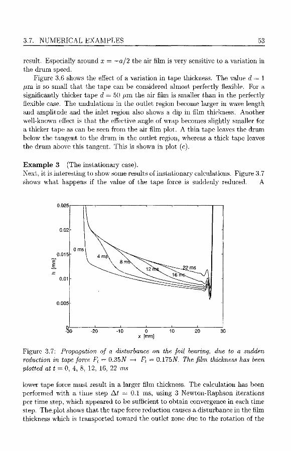
3.7. NUMERICAL EXAMPLES 53

result. Especially around x = -a/2 the air film is very sensitive toa variation in the drum speed.

Figure 3.6 shows the effect of a variation in tape thickness. The value d = 1 µm is so small that the tape can be considered almost perfectly flexible. For a significantly thicker tape d 50 µm the air film is smaller than in the perfectly flexible case. The undulations in the outlet region become larger in wave length and amplitude and the inlet region also shows a dip in film thickness. Another well-known effect is that the effective angle of wrap becomes slightly smaller for a thicker tape as can be seen from the air film plot. A thin tape leaves the drum below the tangent to the drum in the outlet region, whereas a thick tape leaves the drum above this tangent. This is shown in plot ( c).

Example 3 (The instationary case). Next, it is interesting to show some results of instationary calculations. Figure 3.7 shows what happens if the value of the tape force is suddenly reduced. A

0.025r-----r-r----,-----.------,,..-----...,.-----..-----.----.

0.02

0.015

E' .s 0.01

0.005

-~O ·20 -10 0 10 20 30 x [mm]

Figure 3. 7: Propagation of a disturbance on the foil bearing, due to a sudden reduction in tape force = 0.35N -+ Ft O.l 75N. The film thickness has been plotted at t = 0, 4, 8, 12, 16, 22 ms

lower tape force must result in a larger film thickness. The calculation bas been performed with a time step ~t 0.1 ms, using 3 Newton-Raphson iterations per time step, which appeared to be sufficient to obtain convergence in each time step. The plot shows that the tape force reduction causes a disturbance in the film thickness which is transported toward the outlet zone due to the rotation of the

54 CHAPTER 3. THE 01\E-DIMENSIONAL FOIL BEARING

0.02

0.018

0.016

0.014

0.012

Ë .§.. 0.01 .<::

0.008

0.006

j 0.004

0.002

-~O 1

·20 ·10 0 10 20 30 x [mm]

Figure 3.8: Squeeze film behaviour when the drum is not rotating. The initial film thickness corresponds to the one for w 25 rps. The collapsing film thickness has been plotted at t 0, 4, 40, 80, 160, 320 rns

drum. The disturbance ultimately vanishes and a new stationary state remains. Since the drum rotates with w 25 rps, the revolution time of the drum is 40 ms, whereas the disturbance has vanished in about 20 ms. This suggests that a disturbance is transported at half the drum velocity, which is equal to the average velocity in the film. The latter result is the same as found by Eshel an Elrod in [22] for the infinitely wide foil hearing. Another case of interest is the squeeze film behaviour on a non-rotating drum (w = 0), as shown in 3.8. The calculation is started with an arbitrary film thickness, in this case the one corresponding to Example 1. Because of the absence of drum rotation the air film starts to collapse and will vanish ultimately. One can see that the air film collapses the fastest at the inlet and outlet, probably because air can seep out in the longitudinal direction as well there. Compared with the revolution time of 40 ms, if the drum were rotating at 25 rps, the squeeze time is significantly larger; after 320 ms there is still some air under the tape. This explains why rotating heads can build up an average squeeze film on a statie upper drum scanner, provided that the protrusion of the heads is sufficiently large. Similar results of squeeze film behaviour, but only for an infinitely wide tape, can be found in the paper by Stahl, White and Deckert [81].

As far as the author knows, simulations in a lD instationary case including side leakage effects due to finite tape width, have not been presented before in foil hearing literature.

3.7. NUMERICAL EXAMPLES 55

(a) (b) 1 o·3.-----~-------.

10·15'--~-~-~--,___,, 2 4 6 8 2 4

nr. of Newton-Raphson iterations grid level k

Figure 3.9: (a) Convergence of the residual norm in a Newton Raphson process for a stationary calculation, (b} convergence of the film thickness for increasing number of elements

Example 4 (Convergence). The convergence of the Newton Raphson process for the calculation of Example

1, using method A, is shown in Fig 3.9. The number of elements here is Ne1 = 521. About 10 Newton Raphson iterations are sufficient for this calculation method. Due to the under-relaxation in the first 4 iterations the residual reduces only slowly, whereas the subsequent iterations show a fast decay of the residual norm.

Spatial convergence is checked by doubling the number of element,s several times. Consider the following nest of FEM grids

(3.7.1)

where Nk N0 2k is the number of elements on level k (k 0, 1, ... ). The number of elements at level k 0 is here N0 = 130. We study the convergence behaviour by means of the film thickness hk on grid 0%. The grid functions hk and hk+l can be compared by restricting the values of hk+l to the nodes of grid n%, so that the following norm can be defined

1

Il h, Il ~ ( 1: N, ,t,;11 h,(x) - h,+i(x) l' r This number is shown in plot(b) of Fig 3.9 and decreases with increasing grid level k, showing that the solution converges when the grid is repeatedly refined.

Example 5 (Boundary conditions). All the previous examples employed the boundary conditions given in (3.3.9). Ina FEM model it is normally very easy to change any of these boundary conditions. The calculation in Fig 3.10 shows the comparison between the solution with condition (3.3.9) and the solution where we have taken 0( ±t/2) = 0 instead of

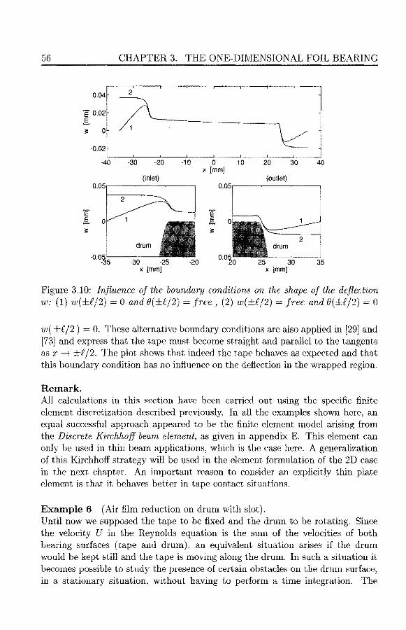
56 CHAPTER 3. THE ONE-DIMENSIONAL FOIL BEARING

0.04 2

Ë 0.02 .s ;:: 0

-0.02

-40 -30 -20 -10 0 10 20 30 40 x [mm]

(inlet) (outlet} 0.05 0.05

2

Ë Ë .s o. .s 0 ;:: 1 ;::

drum

-0.0~ - 5 -30 ·25 -20 25 30 35

x [mm] x [mm]

Figure 3.10: lnfiuence of the boundary conditions on the shape of the defiection w: (1) w(±f/2) 0 and B(±f/2) =free, (2) w(±f/2) free and O(±C/2) 0

w( ±C/2) 0. These alternative boundary conditions are also applied in [29] and [73] and express that the tape must become straight and parallel to the tangents as x--+ ±R/2. The plot shows that indeed the tape behaves as expected and that this boundary condition has no inftuence on the deftection in the wrapped region.

Re mark. All calculations in this section have been carried out using the specific finite element discretization described previously. In all the examples shown here, an equal successful approach appeared to be the finite element model arising from the Discrete Kirchhoff beam element, as given in appendix E. This element can only be used in thin beam applications, which is the case here. A generalization of this Kirchhoff strategy will be used in the element formulation of the 2D case in the next chapter. An important reason to consider an explicitly thin plate element is that it behaves better in tape contact situations.

Example 6 (Air film reduction on drum with slot). Until now we supposed the tape to be fixed and the drum to be rotating. Since the velocity U in the Reynolds equation is the sum of the velocities of both hearing surfaces (tape and drum), an equivalent situation arises if the drum would be kept still and the tape is moving along the drum. In such a situation it becomes possible to study the presence of certain obstacles on the drum surface, in a stationary situation, without having to perform a time integration. The

3.7. NUMERICAL EXAMPLES 57

(a)

0.02

'E É.. 31:

-30 -20 -10 0 10 20 30 x[mm]

(b) 0.01

tape

0.005

'E air film

É..

-0.5 0 0.5 x[mm]

(c) 3

2 m ~1 Q. slot

0

-1 -1 -0.5 0 0.5

x(mm]

Figure 3.11: Infiuence of a slot in the drum surf ace ( a) total view of film thickness (b) film thickness in vicinity of slot (c) air pressure in vicinity of slot

situation with moving tape is a realistic one in for instance linear tape recorders (e.g. computer tape drives).

In the present case we study the effect of a slot in the drum surface, situated in the middle of the wrapped zone (x 0). We take the parameters of Table 3.1 and a. slot with length 0.2 mm, depth 0.1 mm and width equal to the tape width.

In Fig 3.11 we see how the air film has reduced after the tape has past the slot in the drum surface, plot (a) and (b). The relative air pressure drops to zero in the slot, which can be seen in plot ( c), and must be build up again after the tape has passed the slot. It is clear that this air film reduction can be controlled by choosing proper slot dimensions. If the tape drum distance becornes too small, it is necessary to consider the compressible Reynolds equation (and/ or slip-flow), and even the possible contact between tape and drum. A combined

58 CHAPTER 3. THE ONE-DIMENSIONAL FOIL BEARING

lubrication/contact model, in which the tape is partially supported by air pressure as well as a contact pressure may be found in a paper by Lacey and Talke [55].

Remarks. 1. In the present calculations the averaging of the Reynolds equation was car­ried out for the incompressible case. The same technique can be performed for the compressible case, including slip-flow effects (equation (2.4.7)), although the resulting averaged equation will be more complicated (see also [3]). For instance, substitution of (3.3.13) and (3.3.17) into (2.4.7) and subsequent averaging over the width of the tape yields

[! 3 ( 2(n+l)p 6\,)-] _4(n+l)h3 ( 6Àa)--i

1 + 2n + 1 P + h p' x b2 1 + h p -

a ,x

2. Mass inertia effects as considered in (3.3.11) have not been taken into account, although the predictor-corrector scheme can be easily extended for the tape dy­namics case, by using a Newmark method (see Hughes [39]). With tape inertia effects included (see [8J], [38]) the time steps in a simulation must be very small to obtain a good result (about 100 - 1000 times smaller than in Example 3).

59

Chapter 4

The two-dimensional foil hearing

4.1 Introduction

The one-dimensional approach to the foil hearing problem in Chapter 3, has pro­vided a good insight into the lubrication phenomenon of tape on a completely rotating drum. Nevertheless, this model improvement because the simpli­fications in the lD case are too strong. For instance, additional effects are to be expected from the variation of the in-plane tape stress across the width of the tape and the variation of the film thickness in the transverse direction. In this chapter the enhancement to the 2D case is described, following a similar line as in Chapter 3. Firstly, the problem is specified in a more general context, taking account of for instance the helix angle between tape and scanner, the fixed lower drum etc. Next, the complete set of equations for this generalized model is given in its strong formulation. A weak formulation is then derived, starting from the 3D elasticity equations for the Reissner Mindlin case, as given in Chapter 2, in which the tape is considered a..;:;; a "degenerated" 3D solid. fini te element discretization, arising from this weak form, is treated with special attention to a thin plate element with Kirchhoff constraints. This discrete set of equations can then be solved to study the foil hearing behaviour in the 2D case.

4.2 Problem specification

Consider again a piece of tape, with length f , width b and thickness d, wrapped helically around a rigid drum ofradius Rd with helix angle /3 (see Fig 4.1). Elastic constants of the orthotropic tape are the Young moduli Ex resp. Ey in x resp. y direction and the Poisson ratios Vx resp. Vy· The angle of wrap is denoted a, so that the wrapped length a measured along the center line of the tape is given by a cos f3 = aRd. In the present configuration, the drum consists of a fixed lower drum and a rotating upper drum with a circumferential velocity U = 2nwRd, where w is the number of drum rotations per time unit. A uniform tape tension

60 CHAPTER 4. THE TWO-DIMENSIONAL FOIL BEARING

rotating upper drum

Figure 4.1: Unfolded coordinate surface used for the description of a tape wrapped helically around a half rotating scanner

T is applied at the beginning and end of the tape and results in a total applied tensile force given by Ft =Tb. However, more general tension distributions are allowed in this model. For instance a linearly distributed tape tension

T = T(y) = ~t _ 121vftY'

where Mt is a total applied moment perpendicular to the tape, induced by tape guides or other tape path elements.

A similar orthogonal .i:, y-coordinate system as in Chapter 3 is considered here, but now of course wrapped helically around the drum (see Fig 4.1 and also Fig 3.1). The z-coordinate is taken perpendicular to x and y. The inlet and outlet region in this case are determined by the following inequalities

{

inlet

outlet

(x + a/2) + ytan/) < 0,

(x - a/2) + ytanp 0, (4.2.1)

(where lxl :; i/2 and IYI :; b/2). The tape deflection w and the film thickness h are again related by

h = hd + w'

where the drum geometry is approximately given by

cos,(3 + ysin if

if

lx + ytan,81 ~ a/2,

lx + ytan a/2.

(4.2.2)

(4.2.3)

4.3. TWO-DIMENSIONAL MODEL 61

As shown in Appendix B, the metric and curvature tensor for helical surface coordinates on a cylinder are (note the opposite sign of ,B compared with (B.36))

[1 OJ b = 1 [ cos

2,6 sin /3 cos ,6]

aafi = O 1 ' af! R sin /3 cos l) sin2 /) · (4.2.4)

Again, there is no need to distinguish between covariant and contravariant com­ponents of a tensor and covariant and partial differentiation are identical. As in Chapter 3 the radius R must be taken a discontinuous function of x and y ( compare with (3.3.2))

R = R(x, y) {

00 ' if

Rd , if

lx + ytanfil 2: a/2,

lx + y tan PI :$ a/2 . (4.2.5)

implying that baf! = 1/ Rd hd,a/3· The shell equations are formulated in conjunc­tion with this definition of R. As before the transportation speed Ut of the tape is neglected in the analysis. The components of the drum velocity with respect to x and y are

Ux=Ucos/3, Uy=Usinp, U=2nwRd. (4.2.6)

For the fixed lower drum ( where y ::; x tan /3) the drum rotation is absent, that is U = 0. The ambient value of p is Pa and the ambient value of the molecular free path length is Àa. The air viscosity is denoted 77.

4.3 Two-dimensional model

After the description of the main problem parameters and coordinate system, the equations and boundary conditions for the 2D model must be given. The funda­mental unknowns of the problem are the air film pressure p, the in-plane tape dis­placements va, the tape defiection w, the tape rotations ()a and the film thickness h. For the pressure we will use the Reynolds equation including compressibility, slip-flow and instationary effects, see (2.4.7). Tape elasticity is described by the shell equations in (2.3.7) (2.3.8) for orthotropic tape (see (2.2.10) and 2.2.25)), with respect to the present coordinate system and the corresponding fundamental tensors of (4.2.4), while using the definition of R in (4.2.5).

Problem 4.1 (Instationary 2D Foil Bearing). Let n (-f./2, f./2) x (-b/2, b/2) c JR.2 be the set of helical surface coordinates describing the piece of tape under consideration, with a boundary r (x = ±.f./2 , y ±b/2) and let [O, te] C JR. be a time interval. For given numbers f., a, Rd, U, TJ, b, d, Ey, Vx, Vy, Pa, Àa and functions R, hd, Wo and po, find the air

62 CHAPTER 4. THE TWO-DIMENSIONAL FOIL BEARING

pressure p, the in-plane displacements V0;, the defiection W, the rotations 00; and the film thickness h such that in n x (0, te)

( ph3P,a) + ( 6ÀaPah

2

a) ,a = ( Ua2

h) ,a + ä(ph)

(a) ' 1217 1271 ät

'°' Naf3,f3 = O (b) '

lvfaf3,(3 - Q°' 0 ( c) '

Qa,a + ( W,a Na.B ),/3 + ba/3 Na/3 +p = Pa. (d) 1

h hd + w ( e) ,

(4.3.1) The initial conditions to be satisfied are

w(x, y, 0) tvo(x,y) , p(x,y,O) = Po(x,y). (4.3.2)

Again we use boundary conditions in a general form

F on r

v* on NaB N~ on fN", a w w* on f w Qana Q* on rQ, eá ()* on re" ) 1'vla,B n13 M* on fM", (l; a

(4.3.3)

The strain displacement relations are

eaf3 = V(a,(3) - baf3W + ~WaW,13,

"'af3 ()(a, (3) ' Î<> = W,<> Ba ·

( 4.3.4)

and appropriate constit·utive equations for the orthotropic case are

(4.3.5)

in which the material coefficients are summarized in the matrix D of (2.2.10).

Remarks. 1. In the constitutive equation for the bending moments an extra term (bae) has been added to the curvatures, for the same reason as was done in (3.3.6), i.e. before being wrapped around the cylinder the tape is straight ( compare also with (2.2.25)). 2. Defining a lubricant flow similar to (2.4.4)

1271 (4.3.6)

4.4. WEAK FORMULATION 63

the pressure boundary condition in ( 4.3.3) can be written more general as

</>a na = </>* on f,p . (4.3.7)

In this way a no-flow condition ( </>* = 0), for instance along a symmetry line of the problem, may be taken into account. 3. No shell surface loads per unit area are incorporated (Fa = Ga 0, see also (2.3. 7)) implying that the second and third term in ( 4.3.1.d) could be rewritten by means of using (4.3.1.b) as

(4.3.8)

which is to be interpreted as a hoop pressure stemming from an initial curvature (baµ) and an extra curvature (w,a;'.l)· 4. Since the luwer drum is fixed, the tape may be in contact with this part of the scanner. If so, the equations in Problem 4.1 must be extended for the contact case. For the time being, however, we treat the problem as if there is no contact and return to the contact problem in a later section.

4.4 Weak formulation

To arrive at the weal\: formulation of Problem 4.1 function spaces L 2 (0.) and H 1(0), similar to those in (3.4.1) but now with respect to the present region n, must be introduced.

Function sets P, U, V, W, ex and ey are introduced (for every time t E (0, te)), to denote trial solutions p, u, v, w, ()x and By depending on the time t and satisfying the essential boundary conditions. Similarly, weight function sets

U, v, W, ex and eu are used to denote functions p, v, w, Ox and Ou that are independent of t, satisfying the homogeneous essential boundary conditions (see (3.4.2) and (3.4.3)).

These spaces are equipped with the usual inner product. Elements of the Cartesian products S and S of the sets above, are written as column vectors

d = [p, U, V, W, ()x, ()y]T ES , d [p, U, V, W,

With the help of these notations the weak formulation of the different ingre­dients of the theory presented above can be set up.

4.4.1 Reynolds equation

Rewrite the Reynolds equation in ( 4.3. l.a) with the help of ( 4.3.6) as

ph &t

= 0. ( 4.4.l)

64 CHAPTER 4. THE TWO-DIMENSIONAL FOIL BEARING

Multiply a pressure weight function p E P with (4.4.1), integrate over the region n and apply the Gauss divergence theorem 1 together with the boundary conditions for p and p. The result is

1 - dJ dn = 1 -a( P h ) dn + fr -P,a, a P !:it P n n u rq, df. (4.4.2)

At this point, the equivalent of. the B-operator in (3.4.6) for the 2D case, is recognized to be

valid for all d E S and all êï E S. The extra term w p in the integral of ( 4.4.3) arises from the coupling between the Reynolds equation and the out-plane elastic­ity equilibrium of the tape (compare with (3.4.6) and (4.4.10)). The presence of this extra term is explained in the next subsection. Similarly, the 2D equivalent of the C-operator in (3.4.6) is

where we have used that = ~~· 2

4.4.2 Elastic equations

In contrast with Chapter 3, the weak formulation of the tape elasticity equations is not found from the shell equations (4.3.l.b-d). Instead, the weak formulation is derived from the simplified 3-dimensional elasticity equations (like in Chapter 2, Section 2.2), that would lead to (4.3.1.b-d) after integration over the thickness of the tape. In this way we obtain aso called degenerated 3D formulation of the shell equations (for more details in the context of linear shell theory see Hughes [39] Chapt. 6). The obvious advantage of this approach is that shells can be treated more generally, especially with respect to altemative behaviour in the thickness direction.

1Note that if rPa is a solution of (4.4.1), then rf>x + A,y and = r/Jy A,x {for an arbitrary scalar field A) is also a solution. This non-uniqueness of the flow is removed by proper boundary conditions.

2If the drum geometry hd depends on the time t also, for instance in the presence of a moving head, this approach needs some modification.

4.4. WEAK FORMULATION 65

To this end, the full 3D region G occupied by the tape must be considered. This region is given by G = n x ( -d/2, d/2 ), where dis the tape thickness. The boundary of G is denoted S äG. The 3D trial and virtual displacements at any point in the shell are given by

w ( 4.4.5)

As in Chapter 3 virfoal strains are associated with the virtual displacements and rotations

(3) - ba,B W + ~( W,a W,(3 + W,13 W,a) ,

K0;f3 (j(a"B) , "f 0; W,a -

( 4.4.6)

3D strains and virtual strains in the shell can be written as

(4.4.7)

where the quantities ea/3i Kaf3 and /a are given in (4.3.4). Constitutive relations in their 3D form are written as

TiJ Dijkt ( Ekt + E~1 ) E~l3 = - z baf3

0'

0, (4.4.8)

where the coefficients in Dijkl are according to (2.2.10) and E~1 are initial strains incorporated to account for the special form of the moment-curvature constitutive relation in (4.3.5). Using the present notations, the weak formulation of equations (2.1.15) for the tape, in its 3D formulation becomes

where f; are the components of the prescribed load per unit volume in the tape and ti the prescribed boundary tractions (compare with Chapter 2). This specific form of the elastic part of the weak formulation is better known as the principle of virtnal work (Hughes [39], Sect. 2.7). After some calculation it is not difficult to show that the external virtual work (EVW) in the right-hand side of (4.4.9) can be written as

( 4.4.10)

66 CHAPTER 4. THE TWO-DIME?\JSIONAL FOIL BEARING

In the first integral of (4.4.10) the origin of the last term -wp in (4.4.3) is recognized. The left-hand side of ( 4.4.9), representing the internal virtual work (IVW), is written as a repeated integration over n and the thickness. Using a column vector notation for the 3D strains like in (2.2.8)

, 2Eyz] , (4.4.11)

with similar notations for e and e0 , and using the material coefficient matri.>:: D from (2.2.10), the internal virtual work can be written as

IVW = { ld/2 ln -d/2

D ( e + e0 ) dz df2 . (4.4.12)

The inner "fiber integral" in (4.4.12) can easily be expanded analytically, but numerical calculation of this integral by means of a quadrature rule has the ad­vantage that the strain e and the material properties in D may be arbitrary functions of z. In this way it is possible to treat for instance the layered structure of the magnetic tape.

Having formulated the principle of virtual work, it is easy to generalize the expressions for the operators A and F of (3.4.6)

F(d) - { ld/2

eTDe0 dz df2 - { wPa dfl ln -d/2 ln

+ ( w Q* ar + 't, ( f N~ dr lr Q c.=l lrN"

f p</>* ar lr<P

It is easy to show that after expansion of the fiber integral in ( 4.4.13), we obtain the more familiar expression

A(d,d)

which is to be interpreted as the sum of the virtual membrane, bending and shear strain energy ( compare with the expression for A in ( 3.4. 6)).

4.4.3 Complete weak formulation

Now that all operators A, B, C and F have been defined the following weak formulation of the problem can be given.

4.5. TIME DISCRETIZATION AND LINEARIZATION 67

Problem 4.2 (Weak Formulation 2D Foil Bearing). For the situation as given in Problem 4.1 find the solution d [p, u, v, w, ex, ey l T E s such that for all - - - T -d = [.P, 'il, v, w, Ox, Oy] S and t E (0, te)

A(d,d) + B(d,d) + C(d,d,d) F(d),

w(x, y, 0) = wo p(x, y, 0) = Po ,

(4.4.15)

(4.4.16)

where the superposed dot stands for partial diff erentiation with respect to t and the abstract operators A, B, C and F are given in (4.4.3), (4.4.4), (4.4.13) and (4.4.14).

4.5 Time discretization and linearization

Time discretization in the weak formulation is performed according to the implicit Euler scheme, as described in Chapter 3. Again it is necessary to find the Gateaux variations of the operators given in the previous section. We start with the formulation of the first variation of A

dO + k

by virtue of the fact that 8eaf3 = ( w,"' 8w, f3 + f3 6w,"' ) and 8ï?,af3 = 8'?"' = 0, according to(4.4.6), and where Na/3 given by (4.3.5). The first variations of eafJ, "'ai3 and 'Ya in the expression for 8e, are given by

8 8 b 8 118 8 ) eaf3 V(a,/3) - c.(3 W + 2\ W,a W,f3 + W,f3 W,a ,

8"'af3 = 8()(a,/3) , 8% = 8w,a 8()"' . (4.5.2)

Using 8h 8w, the Gateaux variation of B becomes

8B(d, d; bd) k P,a ( h3 p + 6ÀaPah

2) 8 1217 P,a

+ P,a (h3

p,a -617Uah) 8p 12 T/

wbp

+ (3h2

PP,a + l~ÀaPahP,a 1217

617U°'p) 8w dO.

( 4.5.3)

68 CHAPTER 4. THE TWO-DIME~SIONAL FOIL BEARING

When calculating the variation of C it must be noted that d and d are to be varied independently, yielding

bd C( ëî, d, <l; bd) = k p ( ~~) 8p + p (:) bw an .

s: C(-d d d. s:d· ) 1 -( h abp. · afJw ) d" ua ' ' ; u (! p at + p at ~l.

(4.5.4)

In the formulation of the equations for the Newton-Raphson update in the pre­dictor corrector scheme, the variation 8dC of C will be neglected with respect to 8d.C. In the incompressible case it vanishes anyway and in the near incompressible case it is small in a large part of the wrapped region. In addition, the omission of this term only changes the tangential stiffness matrix and has no influence on the actual equations. The formulation of the predictor-corrector algorithm is completely analogous to that in Chapter 3. Suppose that the following quantities are given at t = tn

Pn (4.5.5)

Find the solution dn+1 1 Pn+Ii Wn+I at the next time step tn+I = tn + t:.t by solving the equations

A(d, dn+l) + B(d, dn+l) + C(d, dn+li dn+l) F (d), (4.5.6)

Pn+I = Pn + !::i.t Pn+l : Wn+I

by means of a predictor-corrector scheme. The solution of ( 4.5.6) at t tn+l

is performed in the same way as in steps (3.5.6), (3.5.7), (3.5.8) and (3.5.9) for 8 1, but with the difference that a predictor and corrector step for p~+I must be included in (3.5.6) and (3.5.9) respectively, because the instationary part of the Reynolds equation also depends on p. Also the definition of 6C~+I is slightly different here

6C~+i := 8<l C( ëî, d~+l' d~,-+-i; t:i.<l~+ 1 ) .

To obtain a matrix-vector notation for the functionals A, B, C and their Gateaux variations the following differential operators, the "ID-matrices", are defined (compare with (3.5.10))

ä 0 äx 0 -z 0

0 0 ä äy 0 -z

IB1 = 0 ä a äy äx

a -z (4.5.7) -z &y

0 0 0 -1 0

0 0 0 0 -1

1

4.5. TIME DISCRETIZATION AND LINEARIZATION 69

0 ä 0 (w - bxx) ~ fj 0 äx ,x -,;., 8x

0 0 (w,y /!u byy) 0 -z2-äy

IB2 0 a (w,x +w,y - 2bxy) -z2- -z :x (4.5.8) 8x f}y

0 0 0 ä -1 0 äx

0 0 0 a 0 -1 8y

1 0 0 0 0 0

[ ~ 0 0 0

~ l a 0 0 0 0 0 lB3 lB4 = ax (4.5.9)

0 0 0 ' 0 0 0 0 0

0 0 0 1 0 0

Again, the transpose of these operators is treated as a postfix operation. The following "Il-matrices" are introduced (compare with (2.2.10) and (3.5.11))

E x 0 0 0 1- 1 - V:1Yy

D1 1 1 - V;cl/y 0 0 0

(4.5.10) 0 Gxy 0 0 0 0 G:u 0

0 0 0 0 Gyz

D2 [ Nxx Nyx

Nxy] Nyy '

(4.5.11)

[ ~. 0 0

~ 1 [ ~~ 0 0

~. 1 D3 C1 0 D4 = C1 0

(4.5.12) C2y 0 C1 ' C3y 0 C1 C4y

-1 0 0 -1 0 0 0

where the coefficients in the last two matrices are given by

h3 p + 6ÀaPa h2 -Uo;h C1 = C2a

1217 2

Cao: h3

1217 (4.5.13)

C4o: + 12ÀaPa

1217

h 0 0 p 0 0 0 0 0 0 0 0

D5 0 0 0 0 0 0 0 0 0 0 0 0

(4.5.14)

0 0 0 0 0 0 0 () 0 0 0 0

70 CHAPTER 4. THE TWO-DIMEI\SIONAL FOIL BEARING .

With the help of these definitions the functional A and its Gateaux variation óA can be written as follows

A(d,d) k ld/2 -d/2

dT(IB:[ D1 IBi) d dz dO.

óA(d,d; 8d) k d/2

[d/2 dT ( IB:[ D1 182 ) ód dz dO +

Likewise, the functionals B, C and their variations can be written as

B(d,d)

óB(d,d;ód)

C(d,d,d)

óa C(d, d, d; ód)

(IBJD3181 )d dO,

dT (1B[D11B1 )8d dO,

-T • d Dsd <ln,

4.6 Finite element discretization

(4.5.15).

(4.5.16)

In order to formulate the discrete equations arising from the weak formulation, s and s are approximated by fini te dimensional subspaces sh and sh, as before. We start again by dividing the region n as described in Problem 4.1, into finite subregions ne such that

(4.6.1) e=l

A typical element is described by map ping the bi-unit square ( -1 =::; Ç, rt =::; 1) onto the physical element region, as shown in Fig 4.2. The familiar bilinear shape functions are used to interpolate all unknowns on an element ( a = 1 ... 4)

(4.6.2)

where ea (Ça, rta) represent the values of the element nodes in the parent domain. The global position x depends on the local position e in the following way (in column vector notation)

4

x(e) L Na(e)xa. (4.6.3) a=l

4.6. FINITE ELEMENT DISCRETIZATION

(-1,1)

4

(-1,-1)

Pl 1 1 1 1

paren! element reglon

3

2

physlcal element region

Figure 4.2: Four noded bilinear element

71

T On every element the unknown d = [p, u, v, w, 8x, 8y] E S is approximated by dh ES

4

Na(x) d~(t) , ( 4.6.4) a=l

where d~(t) are the approximate values of d in the nodes Xa of the element. A matrix vector fashion of (4.6.4), equivalent to (3.6.4), is

dh N ue ue T [ di T 1 d~ T 1 d3 T 1 d4 T ]

[ Ni 1 Nz I N3 I N4 ] , N" (4.6.5)

N

where 166 is the 6 x 6 identity matrix. Similar notations hold for ód and d. As before, all integrals can be written as a sum over the elements and the discrete approximations ford and d substituted in the element integrals. Application of the IB operators in (4.5.7), (4.5.8) and (4.5.9) to the N matrix yields the familiar "Il-matrices", that is

('i 1,2,3,4) (4.6.6)

and a nodal partition of Bi can be written as

Bi = [ Bil 1 Bi2 1 Bi3 1 Bi4 ] ' Bia = IBi Na .

Straightforward application of this definition to B3 and B 4 leads to the following expressions (compare with (3.6.10))

Na 0 0 0 0 0

[ ~ 0 0 JV",x 0 ~] Na,x 0 0 0 0 0 B3a , B4a . (4.6.7)

0 0 Na,y 0 Na,y 0 0 0 0 0

0 0 0 Na 0 0

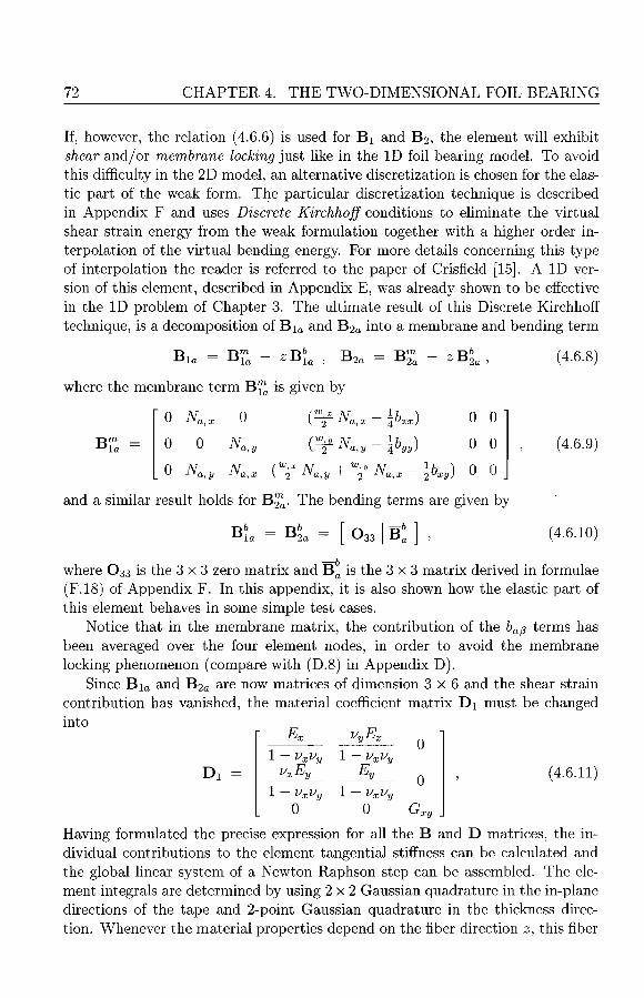
72 CHAPTER 4. THE TWO-DIMENSIONAL FOIL BEARING

If, however, the relation (4.6.6) is used for B 1 and B 2 , the element will exhibit shear and/ or membrane locking just like in the ID foil hearing model. To avoid this difficulty in the 2D model, an alternative discretization is chosen for the elas­tic part of the weak form. The particular discretlzation technique is described in Appendix F and uses Discrete Kirchhoff conditions to eliminate the virtual shear strain energy from the weak formulation together with a higher order in­terpolation of the virtual bending energy. For more details concerning this type of interpolation the reader is referred to the paper of Crisfield [I5]. A ID ver­sion of this element, described in Appendix E, was already shown to be effective in the lD problem of Chapter 3. The ultimate result of this Discrete Kirchhoff technique, is a decomposition of B 1a and B 2a into a membrane and bending term

B1a = B~ - Z BL , B2a = B~ - Z B~a , (4.6.8)

where the membrane term B~ is given by

[

Ü Na,x Ü (W:;!x Na,x - ~bxx)

B~ = 0 0 Na,y (y Na,y - ~byy)

Ü Na,y Na,x (W:;!x Na,y + W2y Na,x - ~bxy)

0 01 0 0 '

0 0

(4.6.9)

and a similar result holds for B~. The bending terms are given by

BL = B~a = [ Û33 1 B: ] ' (4.6.10)

where 0 33 is the 3 x 3 zero matrix and B: is the 3 x 3 matrix derived in formulae (F.I8) of Appendix F. In this appendix, it is also shown how the elastic part of this element behaves in some simple test cases.

Notice that in the membrane matrix, the contribution of the ba/3 terms has been averaged over the four element nodes, in order to avoid the membrane locking phenomenon (compare with (D.8) in Appendix D).

Since B 1a and B 2a are now matrices of dimension 3 x 6 and the shear strain contribution has vanished, the material coefficient matrix D 1 must be changed in to

0 I - VxVy I - VxVy

D1 VxEy Ey Ü (4.6.11) I - VxVy I - VxVy

0 0 Gxy

Having formulated the precise expression for all the B and D matrices, the in­dividual contributions to the element tangential stiffness can be calculated and the global linear system of a Newton Raphson step can be assembled. The ele­ment integrals are determined by using 2 x 2 Gaussian quadrature in the in-plane directions of the tape and 2-point Gaussian quadrature in the thickness direc­tion. Whenever the material properties depend on the fiber direction z, this fiber

4.7. MODEL FOR TAPE CONTACT SIMULATIONS 73

quadrature rule must be changed accordingly. A computer implementation has been written again in the Fortran 90 language, using standard software from the NAG library.

4.1 Model for tape contact simulations

The occurrence of contact between tape and scanner or magnetic heads, makes it necessary to have a model for the description of unilateral constraints. This section describes how to incorporate constraints that arise in a tape contact sit­uation.

A logical measure for detecting whether the tape is in contact with the drum (or a magnetic head) is the film thickness h, i.e. h must always be non-negative.

Consider fora moment the simple case with a non-rotating drum (i.e. U = 0). In this case the quantity Pc p Pa can be interpreted as a contact pressure, that must vanish whenever the tape is not in contact with the drum. If the tape is in contact, Pc must always be positive and this provides a means to decide if the tape must be released from the drum (head) in the course of an iterative contact algorithrn. The contact equations can therefore be described in the form of the following complementary conditions

{

Pc = 0 /\ h > 0

Pc > 0 /\ h = 0

if no contact

if contact (4.7.1)

which implies that Pc h = 0 everywhere. In a computer irnplementation the presence of contact may be checked on a node by node basis. At a given node the contact algorithm has the form

if ( h S e /\ Pc > 0) V ( h S -<::) then h = 0

else Pc = 0 (4.7.2)

where e is a small number. For the simple case U 0, equation (4.7.2) then replaces the Reynolds equation in (4.3.1.a) whereas the remaining unknowns are determined by ( 4.3.1.b-e). Thus, if h 0 the value of Pc is determined by ( 4.3.l.d).

An alternative strategy to treat the contact problem is to add a foundation stiffness term to the out-plane equilibrium equation (4.3.l.d)

(4.7.3)

where

Pc (4.7.4)

In (4.7.4) k1 represents a foundation stiffness, hmin a mm1mum allowed film thickness, for instance to account for surface roughness of tape or drum, and

74 CHAPTER 4. THE TWO-DIMENSIONAL FOIL BEARING

( h - hmin )- = min( 0, h - hmin) is the penetration into the foundation. The latter strategy corresponds with the well-known penalty method to take account of unilateral constraints. Of course, alternative forms of the penalty pressure in (4.7.4) are possible (see for instance Lacey and Talke [55] where the contact pres­sure depends quadratically on the penetration). Because there is a minimum film thickness, the air pressure p may still be calculated from the Reynolds equation in the region of contact, or may be simply put equal to ambient pressure there. Insight in the effectiveness of the algorithm proposed in (4.7.3) and (4.7.4), is obtained quickly by studying the lD situation of example 1 in Chapter 3 for the case of a statie drum, i.e. U = 0. Because of the absence of drum rotation the tape will contact the drum in the wrapped region. The contact pressure Pc must equal the hoop pressure in the contact zone, except for the points of first contact where there exists a singularity in the contact pressure.

The result of such a calculation has been plotted in Fig 4.3. Plot (a) shows the defiection of the tape in the inlet region of the drum (the outlet region shows the opposite behaviour). lt is seen that indeed the tape touches the drum shortly after the inlet point x -a/2. Due to the bending stiffness of the tape the effective wrap angle is slightly smaller than the theoretical one, whereas the tape is running with a slight deviation from the tangent to the drum.

Plot (b) shows the contact pressure calculated with the discrete Kirchhoff beam element as described in Chapter 3 and Appendix E. The following values were used for the parameters in the penalty method in this example: hmin 0.05 µm, k1 100 N/mm3 = 100 kPa/µm (the maximum penetration in this case is about 0.02 µm).

In addition, to obtain a more realistic situation, a one-dimensional head is protruding through a window in the middle of the drum. The parameters for head and window are: window length lw = 4 mm, head protrusion uh 40 µm, head radius Rh = 10 mm and head length lh 3 mm. Plot(c) and (d) in Fig 4.3 show the tape defiection and contact pressure in the vicinity of head and window.

An important observation to be made here is that the value of the foundation stiffness may not be too large, in order to obtain good convergence of the algorithm. This is especially true if the contact pressure is calculated with the Timoshenko beam element described in Appendix D. In this case, too large values of kt result in contact pressure oscillations in the contact zone and very bad convergence behaviour. This is the most important reason to consider a discrete Kirchhoff element instead of the Timoshenko beam element.

Similar observations can be made in the 2D case for plate (shell) elements. The discrete Kirchhoff strategy described in Appendix F has been compared with the so called "Tl-strategy", fora situation like the one in the example of Fig 4.3. This well-known plate element is based on independent shear strain interpolation and described by Hughes and Tezduyar in [42] and by Bathe and Dvorkin in [4]. Again the discrete Kirchhoff strategy shows better results with respect to the

4.7. MODEL FOR TAPE CONTACT SIMULATIONS

5x 10

-3

tape

E' 0

.§. 3:: -5

-1~ - 8 -27

3

_2

"' a. d!:. o1 a..

0

-28 -27

-3 -2

6

-2

drum

-26 -25

-26 -25

-1

(a)

-24 x[mm]

(b)

~ -24

x[mm]

(c)

0 x[mm]

(d)

0 x[mm]

-23 -22

-23 -22

75

-21 -20

-21 -20

2 3

Figure 4.3: Result of 1 D calculation in case of contact between tape and statie drum (U 0) for the parameters of example 1 in Chapter 3 : ( a) tape defiection in inlet region, (b} contact pressure calculated with discrete Kirchhoff beam element, (c) tape defiection and (d) contact pressure on the head

76 CHAPTER 4. THE TWO-DIMENSIONAL FOIL BEARING

contact pressure, than the Tl strategy. An independent confirmation of this different behaviour of thin and thick shell

elements is obtained by performing similar contact calculations with elements from the commercially available finite element package MARC, Version K5.l. In the element library of this package, element 72 resembles the discrete Kirchhoff element used in this thesis, and element 75 resembles the Tl element. Again difficulties occurred with element 75 in the contact area, whereas element 72 showed more stable results.

A final remark concerns the contact situation between the scanner ruler and the lateral edge of the tape. In this case we can use a same contact algorithm as described in (4.7.2), or as in (4.7.3)- (4.7.4), but now with respect to the in-plane tape displacements.

77

Chapter 5

N umerical Examples

5.1 Introduction

In this chapter the computer implementation of the rigorous model treated in Chapter 4, is shown to be a useful tool in the study of tape scanner interface problems as mentioned in Section 1.2. In the following sections some results of case studies are presented. Section 5.2 shows foil hearing calculations for a completely rotating drum, stationary and instationary, and a comparison with experiments. In Section 5.3 similar calculations are shown for the case of a scanner with a fixed lower and rotating upper drum, including the helix path of the tape. In Section 5.4 the results of a statie head-tape contact simulation, i.e. for complete absence of air film lubrication, can be found. Typical results of such a calculation are : tent form, tape stresses around the head, reaction force on the head and head tape distance information. In Section 5.5 we show how grooves in the surface of a rotating drum affect the air film. Grooves are sometimes applied to improve the head tape contact condition. In Section 5.6, a tent form calculation is presented, in case there is a lubricating air film under the tape. The typical phenomena occurring around the head in this case, are also observed in experiments. Finally, Section 5.7 treats slip-flow and compressibility aspects.

5.2 Air film on a completely rotating drum

The first example in this chapter concerns verification of the finite element model for the foil hearing problem, by repeating the air film calculations as presented by the author in [73]. In this paper solutions of the foil hearing problem are calculated by means of the finite difference method (FDM). Tape elasticity is described there by the fourth-order nonlinear Von Karmann equations formulated with respect to the tape deflection w and an Airy stress function tp. An iterative nonlinear Gauss Seidel scheme with time stepping is used to solve the equation

78 CHAPTER 5. NUMERICAL EXAMPLES

system. Hence, the approach in [73] is completely different from the one presented in this thesis.

In Table 5.1 the nominal values for the calculations as given in [73] are shown. Note that these values differ substantially from the VHS parameters used in the lD examples of Chapter 3. The first simulation concerns a 2D air film calculation

a wrap angle 166 degr w angular velocity 50 rps a wrapped length 57.95 mm u drum velocity 6283.2 mm/s f tape length 76.8 mm T tape stress 0.0275 N/mm b tape width 8.00 mm Ft tape force 0.22 N

Pa ambient pressure 0.101325 N/mm2 Àa free path length 0.064 µ,m

d tape thickness 13.0 µ,m T/ i air viscosity 1.81 *10-11 N.s/mm2

Rd scanner radius i

20.0 mm Dt • tensile stiffness 136.71 N/mm Ex Ey Young modulus

1

9570.0 N/mm2 Db 1 bending stiffness 0.00193 N.mm Vx = Vy Poisson ratio 0.3 D 8 shear stiffness 47.85 N/mm

Table 5.1: Nominal values of the calculation parameters in this section

in case the drum is completely rotating and there is no helix angle between tape and drum (i.e. {3 = 0). In Fig 5.1 apart of the nonuniform finite element mesh in the outlet is shown. The air film is taken stationary, i.e. fJh/fJt 0. Because the situation is symmetrie with respect to y = 0, only the lower half of the tape has to be modelled. In the present case the grid is refined in the outlet region, where air film undulations are expected like in the lD case. The element size is also smaller on the lateral tape edge y = -b/2. In [73] it was only possible to calculate on a grid with constant mesh pitch in x and y direction, which immediately shows the advantage of the present finite element method for this type of calculations.

The boundary conditions for this specific example have been chosen in the following way

x -€/2 p Pa' ·u = w Oy 0

x +t/2 p Pa, Nxx T, w = Oy 0

y -b/2 p Pa

y 0 v Oy 0 ( symmetry)

The remaining quantities satisfy the homogeneous natural boundary conditions. Again, methods A and B as described in example 1 of Chapter 3 are applicable

in this case. As in the lD calculations method B seems to be more robust than method A, but is also more expensive. Therefore, a good strategy in this case is to start with method B performing a few small time steps with 1 Newton Raphson iteration per step to settle an initial solution for method A, and then switch immediately to method A,

5.2. AIR FILM ON A COMPLETELY ROTATING DRUM

'E É,-2

-4

15 20 25 30 35 x [mm]

40

Figure 5.1: A part of the finite element mesh for the calculation of the air film on a completely rotating drnm (symmetry with respect to y = 0)

40

y [mm] -40 x [mm]

Figure 5.2: Air film thickness on a completely rotating drnm, with zero helix angle

79

80

0.015

0.01

.t: 0.005

0 -30 -20

0.01

0.008

0.002

CHAPTER 5. NUMERICAL EXA~iPLES

(a)

a :y 0.0 mm b :y= -3.3 mm c: y = -4.0 mm

c

-10 0 x [mm]

c

a : x = -20.0 mm b: x O.Omm c: x = 20.0 mm

a b

10 20 30

b

O'--~-'-~~-'-~~'--~-'-~~-'-~~'--~-'-~--'

-4 -3 -2 -1 0 2 3 4 y [mm]

Figure 5.3: Cross sectional views of the air film thickness: ( a} lateral cross sections with undulations in exit zone, (b} transverse cross sections with anticlastic curvature eff ects at tape edges

0.02

0.015

0.01 'E .§. 0.005

0

-0.005

-O.Q1

40

0 20 0

-20

y [mm] -40 x [mm]

Figure 5.4: Tape defiection w for a completely rotating drum

5.2. AIR FILM ON A COMPLETELY ROTATING DRUM 81

i.e. a very large time step with a suitable number of Newton Rapson steps. In this way, approximately 10 Newton-Raphson steps appeared to be sufficient to obtain a converged stationary solution. In contrast with the simulations in Chapter 3, the present simulations were performed on an IBM RS/6000 com­puter, with a 250 MByte main memory. In addition, use was made of the Fortran 90 compiler available on this platform (XLFortran Version 3.1 , see [44]). The linear equations, in each Ne\\rton Raphson step, were solved by means of a gen­era! "skyline matrix" solver from the ESSL-library (subroutine DGKFS, see [43] Chapt. 10). This solver takes advantage of the skyline structure of the banded stiffness matrix; it uses the columns of the nonzero upper triangular part and the rows of the nonzero lower triangular part in the matrix.

Fig 5.2 shows the calculated 2D air film thickness on the completely rotating drum for the parameters of Table 5.1. We immediately recognize the typical air film behaviour from the lD calculations, i.e. a decreasing film thickness in downstream direction, due to air leakage at the tape edges. Another phenomenon is the cupping of the tape in the transverse direction, where the tape prevents air from flowing away at the lateral edges.

Cross sections of the air film are presented in Fig 5.3. The later al cross sections in plot (a) are calculated for several values of the y-coordinate and clearly show the familiar undulations in the exit zone. The other cross sections in plot (b) give a clear view of the tape curvature in transverse direction, but also reveal an elastic boundary layer phenomenon at the edges y = ±b/2, due to the anticlastic bending of the tape: a well-known result in literature (see Licht [60]). This was the main reason to refine the finite element mesh in this part of the tape.

Figure 5.4 shows that the deflection w of the tape behaves in the same manner as in the lD case: a maximum in the inlet zone inlet and a minimum in the outlet region.

The air film pressure has been plotted in Fig 5.5. One can clearly see that the pressure undulations in the exit region contain more details than in the lD solution: there exists a 'spike' in the pressure towards the edge of the tape. It is clear that a finer grid would be needed to accurately calculate the value of this pressure spike. Although the author did not make any attempt to achieve this, it is clear that the use of FEM is a convenient way to make the necessary local grid refinements. The pressure returns to its ambient value at the boundary of the tape and furthermore, it is independent of x in a large part of the wrapped region. It is also clear from this plot that the pressure shape function in (3.3.17), used to derive the averaged lD model, appears to be a reasonable approximation for the pressure (the average value of the 2D pressure across the width of the tape is indeed approximately equal to the hoop pressure).

In Fig 5.6 the membrane stress in the x-direction Nxx has been plotted. In the inlet and outlet region of the tape, the stress returns to the uniform applied value. In the wrapped area, the stress in the middle of the tape is about 2-3

82 CHAPTER 5. NUMERICAL EXAMPLES

times larger than at the tape edges. At every cross section, numerical integration of Nxx across the tape width always yields the correct value, equal to the total applied tape force Ft. It is clear that this stress redistribution and the transverse shape of tape deftection and film pressure, are strongly correlated.

A comparison of calculation with experiment has been given in Fig 5.7. The experimental data are the same as in [73], where they were used to verify the FDM results. In [29] Fijnvandraat used these values too for the verification of his ID foil hearing model. The measurements were done on an experimental setup equipped with a photonic sensor, by means of which the tape drum distance could be measured. We can see that the present FEM solution is in good agreement with the experiments (notice the undulations in the exit zone). In the transverse cross section of plot (b) there is hardly any evidence of the anticlastic curvature in the experimental data. This is probably due to the fact that the size of the light spot emanating from the photonic sensor, is too large to give accurate results on the edges of the tape. Use of alterna.tive, more accurate optical measurement equipment might resolve this problem, e.g. a non-contact (laser) displacement meter based on a triangulation method.

3

2

IE. 1 =. al 0 a.. 6.

-1

-2

5

y [mm]

0

J__~~----;-~~-----,~~~~20:--~-\40 0 -20

-5

-40 x [mm]

Figure 5.5: Relative air film pressure on a completely rotating drum

A final example for the completely rotating drum, concerns a transient calcu­lation. In Fig 5.8 we see the propagation of a disturbance in the air film caused by a sudden increase of the angular drum velocity ( w = 50 rps ---+ w = 100 rps), which must result in a larger film thickness.

5.2. AIR FILM ON A COMPLETELY ROTATING DRUM

x x

0.04

z O.Q1

0

0.02

0.015

0.01 .c

0.005

0

0.015

'E ..s 0.01 .c

0.005

y [mm] x [mm]

Figure 5.6: Tensile stress in x-direction

(a) air film at y"' 0.0 mm

100 rps

e~~i:!_n_:ent __ 50 rps ------- --~

calculation

-30 -20 -10 0 10 20 x [mm]

(b) air film at x"' -21.64 mm

-------- 100 rps ---

calculation '--~--'-~~-'-~~-'-~~"'---~--"~~

-4 -3 -2 -1 0 2 3 y [mm]

30

' '

4

Figure 5. 7: Comparison of calculation with experiment for different drum velocities (w = 50, 100 rps}: (a) laternl cross section (b} transverse cross section

83

84 CHAPTER 5. NUMERICAL EXAMPLES

0.02

O.ü15

'E .s 0.01 ..c:

-30 -20 -10 0 10 20 30 -5 0

x(mm] y (mm]

0.02

0.015

0.01 ..c:

0.005

0 -30 -20 0 10 20 30 -5 0

xlmml y[mm]

0.02 i

t = 4 ms 0.015-'

'E .s 0.01 ..c:

0.005--

0 -30 -20 -10 0 10 20 30 -5 0 5

x[mm) y[mm]

0.02

0.015

'E .s 0.01 ..c:

0.005

0 -30 -20 -10 0 10 20 30 -5 0

xrmml y[mm)

Figure 5.8: Propagation of a disturbance on the foil bearing, due to a

sudden increase (at t 0) in drum velocity w 50 rps w = 100 rps. The film thickness has been plotted at t = 0, 2, 4, 10 ms

5.3. AlR FILM ON A HALF ROTATING SCANNER 85

Like in the lD case, the disturhance is driven from the inlet. t.o the out.let by the n1otion of t.he drtun, after \vhich a ne''' st.ationary state rcn1aü1s, As in Chapter 3, com1xue with Fig 3.ï, this dist.urbance is lransported at about half the drn1n velocity. ·The present traHsient re.sult seen1s so111e\Yhat sn1oot.her than the oue iu !ï:3J. The results of thts section can be compared with t.he calculations prescnted by the author in [73] a.nd the general conclusion of such a co1npàrison is that the resulr.s are ueux)y equal: \vhich gi,·es confidence in bot.h co1nputar.ion 1uei.hods. ~.\n ünportant advantnge of t.he present FE~,f approach. ho,vever 1 is its abilit.y t.o haudle n1ore cornplex (essentüd) displaceH1ent boundary conditions, as \veil as irregular 111eshes. This \Vas one of the 111ain reasons t.o develop a finite element fonnulat,iou for the foil hearing problem.

5.3 Air film on a half rotating scanner

T·his sect.ion concerns inorc realistic air fihn caJculations, for the case of a scanner \Vith a rotat,i11g upper dru1n and a, fixed lo\:i,·er drun1 (sec also Fig 4.1). Sinü1ar caleulations \vere prescnted in (73]. The s:une nor11ina.l parru11eters are used &">in J'a.ble 5.1. Because t.he solution is no langer synunetric \Vith respect to y = 0: the con1plete tape region 111ust be discrctized aucl the bounda.ry conditions 1nust be changed accordingly. In this spccific cxample the following boundary conditionB haYc been chosen

~; = ±e/2 p = P.' 11/xx T, w Bu = 0

v( ±l'/2, 0) 0

y ±b/2 p = P,

y = -b/2 u.( 0, -b/2) 0

Furt.hc1111ore. \VC e,xplicit.IJ• pur, p = Pa on t.he fixed lo\ver dru1n whereas any friction on 111.is Jlart i.s ncglccted. In contrast wit,Ji the calcnlations in [73], it. is possible he1·e to consider the contact betweeu the rul er and the lower t,ape edge, by means of tJie method deseribcd in the J'revious diapter. •The first example of a rnlculat,ion is shown in Fig 5.9-5.10 where we can see t.he air film on tJie half rotating system for different n1!ues of the helix angle : ,13 0° and {3 = 5°. ~t.\s cxpooted: there exists only a. layer of air 011 the rotatil1g upper drum and tape drum coutact occurs on the Jower drum, lor both helix angles. For the case f3 = 5° it appeared to he necessary t.o adapt the n1e.sh to the trianguln.r shnpe of the lubricated and contact, reglon. Other,vise 1 Jnany tnore grid points are nceded r,o represent t.he fihn thickne~s accurat.ely enongh (this is a great dra,v­back of the FDM met.bod in [73]). A proper d1oicc of the mesh appears t-0 be an Îlnport.a.nt step in all the calculatious any\\·ay, The nn111bcr of 0JenH:.:nts uscd in this c~kulat.ion was 462.3, comprisiug a total of 27738 degrees of frcedom The calculated maximum band width of the stiffness matrix was 299.

86 CHAPTER 5. NUMERICAL EXAlv!PLES

(a) helix angle O degrees 0.04"""=~-------------

!·~,~-02~

~4 -40 -30 0 10

(b) helix angle "' 5 degrees

0.0 """=,··---~·····--~···------,

'

30 40

y [mm] ·40 ·30 -20 -1{1 0 10 20 40 x lmmJ

F'ignrc 5.9: .4ir jilrn 011 a .5can11er tLrith rotatin.g npver drurn and jixed lo111er

rlntrn, jrff different ·110./v.es of the helix anglc: (a) ,[! = 0° fb) ,8 = 5°

Is

(a)

"-~-------,-.~p.----~j

ai•fi~ ~ of----------~"i'r-----------"

!ixed lower drum rotating upper drum

·1 0 y [mm]

(b)

0

(c)

10

~10 0 10 x [mm]

2 3

20 30

20 30

4

40

40

Figure 5.10: (a) Cross secbon of the aii' film on a ha~f rot.ating sc(}.nner (.6 = .5°) at .T 0 rmn, (b} displacC'm.ent v of !.he lowcr tape edge nt y = -b/2, (c) contact vmssure on the rnler at y -b/2

5.3. AIR FILM ON A HALF ROTATING SCANNER

Ë 0,01

.§. o, 3: -0.01

.4 ' -40

la)

0

(b)

30 40

~Z1 0 10 30 40

x 104 (c) ,,.si-~--~--~----~--··

!o-· _ ~---"'=--~ ... __ LL_~J ~ ~ ~ -10 o 10 m m •

x [mmj

87

I:i""ignre .5.] l · Result for a ::;canner nrif.h a rotating upper dr11.1n (,B = 5°) and a fixcd lawer drnm with o. rndi1cç step of 10 1.1.m (a) globo./ mcw of trqJe deftection (b) displacement 1; ot y = -b/2 and (c) contact vressurc on t11.e mier a.t y = -b/2

.A..hout 10 NR steps \\Tere needed: ..,vitl1 an average of± 2 CPU ininutes per st"p. For /J 5° a f.ransverse cross section of r.!1e air film 11t x 0 is shown in plot (a) of Fig 5.10. Becanse of the absence of air on tlm lower drum, the drurn surfacc see1ns effectivel:y cone shaped. Since \VC apply a uniforn1 stress at. ~; = ±f/2 and the transverse in-plane displacement v is onle· fixed at (.T, y) (±C/2, 0), the tape w ill have the tendency to follow a developable path aloug this coue (the so callcd ;;free tape path:: ), Hence~ if the ruler i'> absent in the current configuration: the rape "vaut.s to 111ovc in the ncgatîve y-direct.îon. The ruler, hoVi.:cver, forces the tape t.o remain parallel to the 1'-axis as eau be scen in plot (b) of Fig 5.10 and consequcnt.1J therc ls a reaction force of the ruler on the t.ape~ 'vhich is sho\Vll in plot (c). It must be explicil.ly sa.id here, that in a. real t.apc deck there e:à.s! more complica.t.ed bo11ndary conditians at x = ±f/2, iuduced by remote gniding posts i11 the tape deck. For inst.ance, a line<irly dist.ributed tape tension N,.r at.?;= ±f/2 will definitely affect. the rea(;(.ion force »nd displacement ·1; al. the rnlcr, and also t.he air film thickness ( rccall : "e·11crything dcpends vpon cverything"). More work rcmains to be done to couple the cakulat.ious on the scanner, wit.h the acwal couditions in t.he deck. The present. FEM model appcars t.o be a useful tool for 11

this type of analysis, • 1110 second exa111ple of this sect.ion concerns t.he calculatîon of air fihn

thickness on a half rotating scanner (/3 = 5°) where the radius of 1.he fixed lower dru111 is slight1y s111aller than the one of the upper dru1n. This is co111n1on practice

88

E' ;;_

•

CHAPTER .5 NUMERICAL EXAMPLES

(a) x" ·20 O mm

·0.011-------4 -3 --~2JL ___ ~,--~--co--·~---·~~-~--.J4

(b) X=O.O mm

·0.01 f-----------' ·\ 0 2 3 4

(c) x 20.0 mm

·4 ·3 ·2 -1 0 2 J 4 y [mm]

Figure 5.12: Cross seciions of tlie tape defiection on a ha!f rotating scanner with radius step {a) x = -20 mm, (b) .?: = 0 mm., (c) x 20 mm

fora helical scanner, to obtain a het ter toleraucc with respect to track strnightness (aJ\vays in co1nbina.tîo11 \Ylth a proper adjustn1ent of the t::i,pe gnides before and after the scanner).

Fig .5, 11 shO\VS a globnl viev..· of the t.a.pe deftect,ion on the scanner, fora radius step of 10 /Hn, as well as \:he value of the transverse t.ape displaccmeut v at t.he lo\ver tape edge aud the contact pre>sure on the ruler, Fig 5.12 sho\vs transverse cross sectiou of the ta.pe and drum at diffcren1. positions along the drnm. A remarkable resnlt. is that the tape floats freely above the fixed lower drum in a large part of the wrnpped region, which is caused by the rMction of the rnle1 on the t.ape (in absence of the rul er the tape is likeJy to touch the lower drum). This pheno1nenon is a)so observed in expcrilnents. As sa.id: a,:ny friction in t.he contact zone on the fixed lower drnm is neglccted (friction can influence the resnlt). By mnltip1ying the contact pressurc 'vith a friet.ion coefficîent a first guess for this friet.ion is possihlc.

lt. is important to mcutiou here tlrn.t for the calculat.ions presented in this ;;ection, it can son1eti1nes he extre1nely dïfficult. to obtain a convcrging Nc,vton R.aphson iter;Jtion, In t.his case a continua.tion technlque 1 'vhere severaI para1nc­tcrs of the prohlcm are slowly approaclling their ultimate valnes, is the only way ont of thLs problem For cxample, dunng a calcnlation for a drum wit.h radius step, t.he value of the radius step is grnduall" increascd towards its final value. i-\nd of course sn1all titne sceps n1ay be taken at the beginning of snch a calcu­lation (son1etilnes in con1hination "''ith undcr relaxatlon in the Ne,vt.on Raphson

1

!

0

t b

5.4. STATIG HEAD TAPE CONTACT S!MULATIONS 89

update). Other quantit.ies to be played wit.h ;i.re the foundation st1ffness and tlucknes~ occurring iu a contact situation.

5.4 Statie head tape contact simulations

In Chapter 1 ït \Yas rneutîo11ed that the quality of the head-ta.pe contact condition is one of the 1nain issues of the n1echanical aspects of helical scan recording. In this sect,io11 \ve present n head-tape contacr. sin1u]ntion in a statie situation) i.e. for a. non·rotating dru111 (a statie shnulabon is n1ore econon1ic fro111 a co111putat.ional point of \'ie'v than a sirnulation inch1<ling a_Jr fihn effects). Since t.he area occupied by the head is rat.her s1na1l \Vit.h respect. to the total drn1n arcH, it is n<>cessa.ry to perfor111 the calculatiou on a n1esh t.hat is concent,rat.e<l around the he-ad.

In Table 5.2 the nomina! values for these cakulations am shown. They are almost the same as t.he VHS parameters used iu the JD examples of Chap1.er 3. In tJ1e calculations \Ve .:.-onsider a stat.ic dru111 eg11ipped \Vit.h n head \VilH!0\\' 1

"Tap anglc 90.0 degr Q wrappe.ëC lcngth 48 7 lUHl

tape lcngth ï0.3 UHD T tape stress 0.0277 N/1nn1 l.ape \vidLh 12.65 nun F'. tape force 0.35 N

d tape t hickness 15.0 /J.IH R J scanner radius 31.0 ll11U

D, tcnsi!e st.iffness 122.0 N/nun ! E_, )'oung n1odulus ï400.0 N/1111112

D,, bc.nding st iffncs2 0.00229 N.n1n1 v, Poisson ratio 0.3 D, shear st.iffuess

i 42.(19 N/ninl e.

bw !

"'inclow •vidth LO ll)lll t, b1i hcad ,"·Jdt.h 0.1 nun Ui

wiudow lcngth 4.0 IJlHl

head length 3.0 nnn hcad protrusion 35.0 /flil

ltm;.1 : foundation thickua<;s i 0.05 µin k

J?.'T i hcad x-radïus 15 HUU R fo1u1rlat.iou ~tilfncss 119.0 :N/1n1n3

hc<ld ·y-radil!~ 2 Hllll '!! .... ~---~--

Table 5.2: Nomina/ va/ues for a statie /1.ead-tape contaä analysis

t.lirough \\'hid1 a head protrudes. Both window and heacl arn centcrcd with respect to "' y = 0 and thcir spccific dimensions can he founcl in Table 5.2. The tot.al number of element.s in 1,his calculatfon is Nc1 4160, containing totally 26082 degrees of freedom. The band width of the stiffuess matrix in this case was 347.

In Fig 5.13 \Ye can see apart of the finit.e elen1eut 1nesh around a head v.:indO\\' with a protruding hcacL The griel lines are taken such t.lmt the window and ltead tlre represent;ed in a sntisfactory 'v~v. BE'causê of obvious syn1111et.ry: only the lo"·er half of t.he tape has to be modcllcd. lt is immediately secl! that. because of the. s1nall \Vidth of the head there n1ust be a concentration of grid lines a.rouud 'Y = o.

The resull.ing tape def!ect.ion aronncl t.he liead is shom1 in Fig 5. H.

90

N

0.04

-0.04

·0.06

·0.08 0

CHAPTER 5. NUMERlCAL EXAlvlPLES

·0.5

y {mm] x {mm]

Fignre 5.13: A part of the fimte element mesh for o lieo.d ta/lc contact .,imulation, containf:ng a mo.qnclic head and scan.ner windoui (syrnrnetry 11nth rt-,spect toy = 0)

VHS tent torm

•

4

y [mm] .4 .4 x jmm}

Figure 5.14: T<2pC defiection ("tent form") fa tlw vicinity of !he head

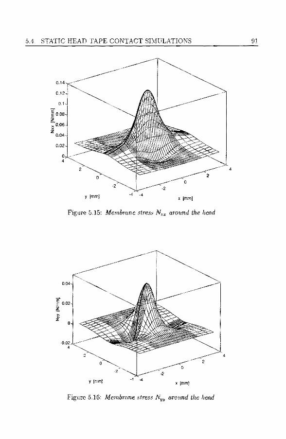
5.4. STATIG HEAD TAPE CONTACT SiiVIULATIONS

0.14

0.12~

01J JooaJ

)<; 0.06j x z

0.04

0.02

0 4

0

y lmml x lmmj

Figure 5.15: Membnmc sl.ress N,x arnund the hcnd

Figure 5.16: Mernbrnne stress Nyy aronnd the head

91

4

4

92 CHAPTER 5. NUMERICAL EXAl'vfPLES (a) norilinear ca:culatîon

!_:::f ff(U:c~ di~anc•~~-· S? )~)IJ ·LS ·1 ·0.5 o o.5 1.5

(a} linear calculation

! : ::f (( ((§?::::::::::. "" ~dislançe;;;< 50~n--n~~::::::::::.... :::::::::.::~D )'Jn_); )i

'

-1.5 ·1 -0.5 0 05 l.5 x fmmj

lbl 0.04~-----,.---~----.-----~----,----,

•• -0.5 0 y [mm]

(c)

lape

0.5 1.5

O.Q4~---~ ----~--·-~-- ·~---~--1

- 0.02

! 00:~-dru_m_-<_ head ~---~-~··D .3 ·2 ·1 0 2 3

x [mm]

(d)

0 0.06 0.08 0.1 0.12 head prolrusion [mm]

Figure 5.17: {o.) Conto11r lincs of head tape dv;tancc on the head (contom· levels. 0.05, 0.2, L2 ,3 ,4 1im), (b) tran.werse crns.1· section of the tent at 2: = 0, (c) iateml cross secti()n of the tent at y ~ 0, {d) head force versvs head 11rot.1·1J.sion characf.eristic

5.4. STATIC HEAO TAP.E CONTACT SIMULATlONS

20

l " ~-- prese0t sludy

16 • "' Jo " •• experimenl (Bèrson)

14 -------· linear model (Bensm;) J ,

12 / ~ ~ 10

" • E" 2400 Nfrnm*'2 ., nu"' o_s d"Q]60mm

4 R"' 12oomm T ""0.676 Nlmm

2

__J 00 0.5 1.5 2 2.5 3

protn.Jsion [mm}

Figure 5.18: Tent. pole force versus protrusion for Benson case C

The sl111.pe of the tape resembles that of a cloth supported by a tent po]e and is therefore calkd a 'tent form', lt can be clearly seen that the in-plane tent din1ensions are already jn the rnrn range \vhereas the valuc of the protrusion is just 35 ,u.111 in 1Jlis case. The protrusion is ho-.,vevBr nearly t\vice as larg-e as the thiclmess of the tape and at. this point t.he need for the use of a geometrical!y nou-Hncar thcory beco1nes clear. Au illustrat.ive t.rea.t1nent of this observation may be fonnd in Timoshenko [Si], Chapt, 13 (on lmge dellections of plat.es),

Fig 5. 15 shows the distribution of the in-plane strnss iV" in x-direction. There exlsts a clear stress t;Oncentrat,ion aronnd the head (about 5 tin1e...::; larger than the tuüforrn applied stress): 'vhereas {).\VU;Y fro1n the head (along the y-dircctjon) the stress ]evel beco1nes lO\Yer t.han the nniforn1 a.pplicd st.r~..ss at the beginning and end of t.he tape. Obviously this is cans(~d by the fact that in every cross section (:r, = constant) the stress rnust be in equîlibriun1 \Vith the unïfortn applicd stress.

The membrnne stress N," shown in Fig 5.16 has a similar behtn~our, but now the stress minimum occurs along the .?J-axis (the total applied in-plane force in y-direct.ion on the tape vaJüshes).

In Fig .5.lï more details of the head tape contact are preseuted. Plot (a) shows contom lines of the head to tape distauce in the rcgion occupicd by the head (contour levels: 0.05, 0.2, L 2, 3, 4 11.m), !or the geomel:rically nonlinear and linear case, respcctively, This linear clastic model is obt.ained from the nonlinear model, by omitting the t.erm (w, 0 N0 a),a in (4.3.Ld) and the term ~w. 0 w,5 in (4.:3.4} \·Vhere the distm1ce becomes smaller than O.o:> 1nn, the t.ape is considered to be in contact with the head (h",in = 0 05 1m1). The hMaJ· model prcdict.s a contact region \\'lüch is lonf,1er and HB.J.TO\vêr thau the one of t,he nonlinear ca.lculation.

94 CHAPTER 5 NUMERICAL EXAMPLES

On the head, the vah1e of the~ foundation stiffness k1 is cakcn su bst.a.ntiaJIJ1 larger tban Oll the drun1: because in t;he head-tape contact region t,l1e peuet.ration of the tape inl.o the foundat.ion must 1101, hccome too large (o.g. smaJir.>r t.ha.n 0.02 pm).

Ploos {b) and ( c) show cross sections of the 1.cnt :Llong ei: 0 and y = 0 respect.ively. Cross sect.ions of the li11ear calculat.ion (not shown) appeared to be ncrn·ly the same as r.110se in plot. (b) and (c). Therefore, if only t.he teut shape is of interest: the present Nev1:ton Raphson schen1e could be acccJeratcd by t.aking account of the fnct, t.hat the elastic part of the tangentlal stiff11~-1>S HHJ,t,rix is al,vays the san1e in a geo111etrically line.rtr 1nodel (e.g. hy- statie condensation: Huglu~· ... s [:39]).

In papers lï6] and fï5]. bv Sakai et aL experiment.s have been conduct.cd t.o 1nea.sure the head to t.ape dîst,ance h,r u~ing a light source in co1nbînatioH ,,..ith a glass hcad or trnusparent t.ape. In chis 'Yay; contour lei:els, like in plot. (a). can be i11ade cxplicitly Yisib]e iu the fonn of int.erferencc fringe patterus. A" qualit.Plti,-e co1npariso11 'vith these 111oasurc1nents indicat-es that, plot (a) is a realistic piet.ure of the actual hcad tape dista.llce ou a 1nag11etic head. Experilncnts and tent calc.ulations (Jikr, the ones here), hut \Yit.h specïnl rega.rd to he<:id \Year: \\'ere present.cd by Broese and Fijnvandraat in [I.3]

lt is also of importance to know the force exertcd by the tape on the head. ln Fig 5.lï (d), we see the oul.-J)lanc head force (in z-clirecl.ion) as a function of the head protrusion. Ou]y for s111all protrusions this relat.ionshî1> inay he c.:ousidered }jne8.r; lJut for protrusions larger than the tape thic.:kness t.his is uo longer iTne.

The necessit;y fora geo111etrically nonJînear n1odel hecotnes again <îpparent. Notice th;i,1, 1.he slrnpe of t.Jie curve in plot (cl) changes from conve.-< ini.o concave as the prot.rusion hecomes t.lrnn 90 11111. The prnt.rnsion of the head ha.s become so large there_, tlun. the tape îs con1plet.ely lifted tt\vay froni the <lru111 over it~s

comp!ei;e widr.h, leading to a different hend force behaYiour. To obtah1 an iudependent confir1natioa of the corrcct.ucss of the prei:ionf.

results~ a calculat.ion has been pcrforn1ed for paran1eters t.aken fron1 a pa}Jer b>· Benson [7]. Ju t.lris pa.per a geometrically linear model is presente<! for the calcula.tion of a t.ent form in t.he presence of a point lond. ln addition, expcrimeutal values a.rc.: given for the vcrification of t.his 1nodel. f'ig 5"18 sho,vs the resnlts for Benson's case C in [ï]. The para.met.cm of the problem in 1.his case me: E = 2400 N/rnm2, /.' 0.3, d = O.ï60 rn111, R" = 1200 mm and T O.GïG N/mm. The dashed line in the plot. reprnsenls t.he result of the linear calculation model in 1,7]: the ast.erisks are the experï111enta.l data of [7] n.nd t,hc solid llne Is the resulL of the present FEf\1 111odel. 'Ihe three curves are nearly equa1 for procrusions

up to one plnte thickncss. For largor prot.rusions the geornetric.-ill,v lîne.:ir n1odel yields t.oo small n1lnes of the point loart, whercas tlw present model is in excellent agreement. wit.h the e.xperimenr.nl dat.n.

.S.5. AIR FILM ON DRUM WITH GROOVES 95

5.5 Air film on drum with grooves

The next case stHdy concerns the învestigat.îon of the iuftuencc of grooves in the dru111 surface. In Chapter 1 it \vas already n1entioned that so1netin1cs it is necessary to reduce the air film thickness, in order to improve the head tape contacL In this section V.'e sho'v the effectn·eness of a grooved dru111 'vith re.5pect. to air filrn reduction. Consider the situa.tiou of a cornpletely rotating drurn

1 uu1nber ·ör groov<:s groove \vidU1 groove deµth

distance

4 ; 0.1, 0.15 ! 0, 2·5; 50: 75

L6

nun tiln 111111

Table 5.3: Vid11es of the groo·ue dimwsions in tlris section

{a} geometry of grooved drum at x = O

0 11 0.05~

!,~~---···~ ·O !4 ··--3~-~-

(),015

"E 0.01

s. ~0.005

0

'

r 1

L ·30

·2

1

,, 2

"---

-20

1~ l? ~ °'

• 1 0 y [mm]

(b) air film at y

groove depth = o.bs rnm

groove widrh = 0.10 mm "'I

drum

j 2 3 4

0

groove width = 0.1 mm

3 ~ ~ 4

' . . . ' 1 "

·10 0 10 20 30 x [mm]

Figure 5.19: (a} Geomet:ry of groove.s at :r = 0 {b) latera.l cross sections of air film at'!/ = 0, for bg = 0.1 mm a"d hg 0, 25, 50, 75 µm (cases 1,2,3,4 respc,ctiuely}

equipped with equidistant, V-shaped grooves of width &9 and depth h9

(sec also Fig 1.5), for the same parnmct:ers as in Section 5.2 The dist.ance of the groove centers is denoted d9 and the number of grooves is denoted N.. The values of

96 CHAPTER 5. NUMERJCAL EXAMPLES

(a) air film at x "'0

- :=------._1

.c 2

~~ groove width = O. 1 mm

' -3 -2 -1 0 2 3 4

y [mm)

s' 10·3 (b) air film at x ~ O

6

.c

---------;c3---~ groovewldth~--------~~ '

o~-~--~--~--'---"--~--~-_J -4 -3 -2 0 2 -1 3 4

y [mm]

Figure 5.20: Transverse crnss seclions of air film o.t x = 0 for va"ious valîtes of grnove width (a) b, = 0.1 mm , (b) b8 = 0.15 mm. The groove depth in cases 1,2,3,4 is resp. h9 = 0, 25, 50, 75 11m

these paran1cters are given in "fa.bie 5.3. i\gain. the proble1n is synunetrlc \Vith respect t.o y 0, so that only one half of the drum (containing 2 grooves) has to be modelled. To rnprcsent t.he grooves correctly a fiuite element mesl1 is needcd \Vlüch c-onta.ins ut least. 3 griel li11es in each groove.

Figure 5.19 sho\VS a ~ransverse cross section of the grooved drurn and Iateral cross sections of t.he air film at" 0 for b8 = 0.1 mm. Not.ice tbc m·ernll reduction of air film thickness. The grooves seem t.o have the largest. inf!uence at. ent.rance and exit region of the drum (possibly bccause more air can flow away there).

Figure 5 20 shows the air film thiclrness in the middle of the drum, i.e. at y = O. ln plot (a) the groove width is b9 = 0.1 nm1 and t.he groove depth takes on the values h

9 = 0,25,50,75 pm. In plot, (b) we sce that if b9 = 0.15 mm

this influence is even larger ,vhere;ns for h9 = 75 µ1n tbc geo1netry of the drn1n becomes visit:>le in the shape of the tape deflect\on w.

As expcctcd, the groove depth has a significMt influcnce on t.hc film and it is clear r.hat a ~Toug ditnension of these grooves can con1pletcly destroy the !ubricating air film, which lc1als to contact and heuce friction bet.ween tape aud

rotat.ing drunL The author has not made additfonal at.tempt.s to simulate t.he effect of grooves

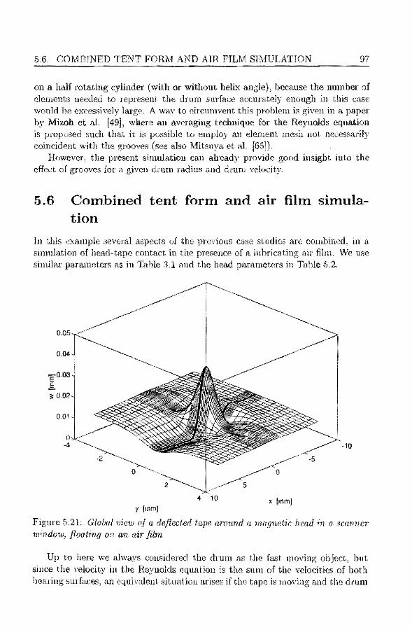
5.6. CO!vlBINED TENT FORi\-1 AND AIR FILM S!MULATION 97

on a half rotat.ing cylinder {with or without helix angle), because the number of elen1ents needed t,o represent. the drnn1 surface accurately enough iu this case \Vonld he excessively laTge. A \\tay to circun1vent this problen1 is given in a paper by Mizoh et aL [49], where an averaging teclrnique for the Reynolds equation is pToposed such that it is possible to en1ploy an elen1ent me ... :-:h not necessarily coincident wit.h the grooves (see also l"vfüsuya et :tl. [65]).

However, the present simulation can aheady provide good insight. into the effect of groove.5 for a given drun1 radius and drun1 velocity.

5.6 Combined tent form and air film simula­tion

ln this e.'>:aniple several aspect.s of the previous case studies are co1nbine<'L in a sin1ulat.ion of head-tapc contact in the presence of a lnbrlcating air fihu. \i\ie use similar parameters as in Table 3.1 and the hea.d parameters in Table .5.2.

0.05~

004J ~

0.01

0 -4

y {rnm]

-10

4 10 x [mm]

Figure 5.21: G/obal view of a de.flect.ed tape arorm.d a magnetic head in o 8cmmer 1uindotJJ" fioa.ting on an air fil?n

Up to here wc always cousidered t.he drnm as the fa.st. moving object" but. since t.he ,-elocity in the Reynolds equatiou is the sum of the velocities of both hearing surfaces, an equivalent. situation arises if the tape is 1110\·ing and the drun1

98 CHAPTER. 5 NUMERJCAL EXAMPLES

is statiouary. This is a simplc trick t.o study the combination of air film and liead tape cont.act, \Vithont, perfornüng a costly tüue integratiou process în case of a moving head. The Jatter is of courSe possible, hut to obtain reliahle !wad to tape distance info1111ation: n1esh rez,oning is necessary al every tüne step to adapt the inesh in the location of the head. The trick >vith the n1oving t;i,pe \Va.s first uscd by Yoneda mHI Sawada in [93:. in case the head is rnprcsented by a sirnple point load. The disad vantrtge of this trick is that. phenomena around t.he liead, seen in the longît11dinal direetio11 of the dru111 1 are reversed \Vith respect to scanner entrance and exit. l'or a. hea<l in the 111iddle of the 'vrapped region t.his is only a 1ninor inconsist,eucy: t.he 111ain peculiarities of the air fil!n around heHd and \\'indo\v \v·ill occnr anyhov.· The san1e 1nesh as in Section 5.-4 \VftS used in the present calculation. In Fig 5.21 we can see t.he deftect.ed tape surface around t-he

(a) 0.04-. - --

0.03- ~···· head motion

E 0.02:-front wave

É.

• 0.01 depression wake

d<um

-O"Oi -8 .s -4 -2 0 2 4 6 8

x [mm)

(bl

window depression wake

--6 -4 ,2 o 2 4 6 a x (mm]

Figure 5.22: Laternl cross section of (a) tape de{lection (b) air pressure at y 0

inagnetic head în the scanner \\'indow (co1npare \Vith Fig 5.14). Th€: tent for1n has a considernble influence on the shaµe of the air film around t.he liead. For inst,auce. \\'e can see a sort of bo\v : \vave 1 in front of the head and aJso a \vake in t.he t;·ai!ing zone of the head. This can be seen more clearly in plot (a) of Fig 5.22. The air pressure is equal to its ambient valne in the liead window, as

can be seen in plot. (b) of Fig 5.22. Tlüs is also t.rue on the he"'L i.e. air film effecr.s have not been considered on top of the heH<l.

In practkc, the shape and dimensions of the head window, must be cl1osen

5.6. COMBINED TENT FORM AND AIR FILlv! SlMULATlON

(a) 0.04:···· --,-----~--..----~-~·

0.03c

E" 002f .§. : tape J: 0.01 '

drum

air mm

-o.o:4~~······-.3~-·-~.2---.··1·-~~o-~······'·--···2~--3~-~.

y fmm]

m "-à. 1 F------

(b)

window 0• ·3 ·2 ·1 0 2 3 4

y fmm]

99

Figure 5.23: 1hm.sverse cross section of (a) tape defiection (b} rclative air pres· Bure at x = 0

~ \

Fîgme 5.24: G'lobal !'iew of a. measmed tent öhape on a VHS scanner

100 CHAPTER 5 NUMERICAL EXAMPLES

in such a, way that the tape is not sueked into the window behind the head, hecause tape-dru111 contact on the rot.ating dru111 ca,n cause tape \VCn.r and/or da1uage. Because the effects due t.o the pressure drop around the \Vindo\v change tJ1e shape of t.l1e t.e11t, they also have influence on the head t,o tape distance whicl1 is anot-her reason to carefully select. the geo111etry of the \VÎndo'v.

ln Fig 5.23, \Ve can see a transverse cross section of the tent and air pressure. A tent shape on a \lHS scanner int.he preseuce of air 1 has b~u 111ea.sured in the sa1ne \vay as the experünentAl air fihn data in F'ig 5.7. A global vie'v of this tent shape has heen plotted in Fig 5.24. One can clearly sec the wake at. the trailing edge of the head,

The experiment has heen pcrformed on a rea,J VHS scanner with a fixed lmYer aJ1d upper drun1 arid one can clearly see t.he thicker air fihn in the rotat.ing upper dru1u. Since in the present. calculation t.here is no fixed lo\ver drun1 1 the comparison of Fig 5.21 with Fig 5.24 can only be qualitative,

5. 7 Compressibility and slip-flow effects

In this final exan1ple \ve study typical phe1101uena occurring in very thin air fihns. ~f'hese exist for insta.nee in the case of linear recording on tape strearr1er beads 1

where the tape moves fast along a stationary head and tracks are \Hitten parallel to t.he tape edge. R.ealistic calcu]ation para1neters for such a case are given in Table 5.4 Here t,lie radius Rrl of the heru:l and the tape force F, are s11d1 that, the

Tiwrnp angle ! 10 dègr u t.a1>c vC!ocity 3000,0 îTifn/s rappcrl lr:ngth t.04ï llllU c tape length 2.094 HUH

tape stress (] l JU2 N/unn b tape \vidth 6.35 n11n

1 , tape force 0,7 1' P, ;unbient pn~ssurc 0.101 N/1111112

: À" : free paih leng! h 0.064 µHl d t<\pC thkkuess 13.0 ;on

1/ air vl15cosit.~v l.8Ii<l0- 11 N.s/1111n 2 R.r1 hca<l radius G.O Jnrn

Ex =E,., Yonng 1nodulus 8000.0 N/nun2 D, tcnsilr; stiff1iess 114,:l N/n1rn

fl:;· =fly Poisson ratio (),3 D, bendîn?. .. stJffness 0,00161 N.llllH -····---

Tn hle fiA: Calculatüm parameters for a linear rfOconhng case

A.ir fihn on the hea.d is in t.he sub1nicron range. In Fig 5.25 calculation result:~ can be fouud for the preseni, cicse, Plots (a) and (b) show air film cross sections for three different fonns of the R1',ynolds c,quation: thé incompressiblc c;isc without, slip-flow effeds ()1, 0), and the eompressible case with and without sli1}-fiow. One can sec that. boU1 <:ompressibility and sliJ}-flow reduce t.hc air film thickness, \Yhere reducr,ion due t.o slip~fto\v is already rather do1ninant here. To explain this, rC\\Tite the st.a.tionar.r~ con1pressible Reynolds equa.tiou, inclnding slip-fto\v

.5.7. COMPRESSIBILITY AND SLIP-FLOW EFFECTS

1 ~

{a} air mm at y =- o.o mm

1 ; incompressible, no slip flow

2 compressib!e, no shp flow c i

!OBL: 0.6

.L·---~---

3 : compresslb!e, wilh slip flow 2

3

···-~-~--~-

30

~ 20

" 10 ll. 6.

0

·0.6 -0.4 -0.2 0 0.2 x_ [mm]

(b} air iilm at x = 0.0 mm

3

·2.5 ·2 -1.5 • 1 y [mm]

{cj relative air pressure at y" o mm

.3

·10-~.,---~-------~

·0.6 -0.4 ·0.2 0 0.2 x [mm)

101

·0.5 0

0.4

Figure 5.25: Cross sectional views o.f the air film tl!icbiess ( a} at y = 0, (b) at x = 0 and (c) relative air pressurc p - P0 at y = 0 , for various .fo-rm.s of the R"ynolds equ.a.tion (labels 1,2,3}

effects, in t.he followiDg form

[ 3 ( P 6Àa ) ·- l h l +Po+ h P,o ,a =

\Vhere jJ = p - P0 is the relat.ive air pressure. Fron1 this expressiou it can he - 6.-'

concluded t.hat if the t.enn ; + ) " is small wfth respect to unity, we regain the a

incompressible Reynolds equation. A characteristic value of pis the boop pressure

102 CHAPTER .5 NGl'vlERJCAL EXAMPLES

T /Il,,. From Table 5.4 we find for the ratio of the hoop pressure and ambient. pressure: T/(PaRd) 0.182. A characteristic rnlue for the incompressible film thickness in this example is H = 0.7 µm and thus 6),a/ H = 0.549. This shows \vhy contrîbut.îon of slip-tlO\v effects to the pressure is significant) if con1pared \Vith the contribution of the ave.rage hoop prcssurc:.

Plot (a) also shows tha.t in the comprcssible C>•se, the amplitude of the imdu­lations in the exit. region decre.a.scs .. .\ si1nilar observation \Vas n1a.dc b_y Eshel in [21 J for the pcrfoctly flcxible lD foil bearing. Eshel pointed out that, eventually, the undula.tions disappenr co1npletely \Yith incroal}Îllg vH.lne of the con1pressibility parameter T /(PaRd).

Furthermore, plot (b) shows that over a large part of the tape width the air film behaves as for the case of infinitely wide tape. Calculations with !.he ID model of Chapter 3, indced prodnce the same air film result at y = 0 in the incompressible case. Moreover, a similar lD model including cornpressibili!.y and slip-flow terms (hut wit.hout side leakagc effocts), also prodnced t.he same resnlts for the oi.her cases in plot. (b).

In addition, plot (b) shows that anticlastic edge effocts are vcry concent.rat.ed at the tape edge, due to the rclatively small value of the head radius. The present resnlts are comparnble to the oues by Heinrich et aL in [38] and i3ï]. In contrast wit.h the results in this scction, the 20 results in [37] do not match the lD calculation for 11 = 0. This is probably due t.o t.hc fact that the author in [37] only considered a constant tape tension: i.e. no tape tension redist.ributiou due t.o air film effects.

Plot (c) shows that compressihifü.y and/or slip-flow effeets ha,·e very lit,tle influence on the re]ativc air pressure.

For a real recording head, the air film in this case canses a t.oo ]11.rge head to tape dlstancc (which should be less t.Jmn about. 50 tHmometer). Therefore, in practice, the air fihn is 11orn1aJJy rednced h.Y app]ying sJots or groovf'"'> in the head e.outour (sec [37], the last exmnple in Chapter 3 aud Scetion 5.5). In t.his way, slip-flow effocts bceome eve.n more important as well as (partial) head tape cont.ac1. phenomena. A second order slip-flow model tlrnt could be useful t.hen is (Mitsuya [64])

S!milar considerations ase valid for an air film mlcnlation on the heMI of Se°' tion 5.6.

10:3

Discussion

In this thesis rnodels have been presented for the simnlation of tape-head-scanner interaction in he1ical sca.n recor<ling. _A,.. lD as \Yell as a 2D finite ele111ent inodel appeared to be valuable tools in the studv of this interface_ Results of calcu­latious shou-n in t.he pre·vlons chapters~ appeared to be in close agree111ent \Vith calculations and/or experünents presented in ear1ier publications. The rigorous 2D ele1nent- for1nular,ion acc-ount.s for rnany aspects, like instationary ef[octs: ge-01uetrically nonlinearity: tape ort.hotropy: cont.act, bet,\vee11 t.ape: head: scanner and ruler~ the heli.-;: pat.hof the tape as \Ve11 as alternative sca.nner profilcs,

The a<lde<l va.lue of the study in t.his thesis Js a ncvJ fiuite ele111ent for1nulation for this problem, where use has been made of an e.'<plicit thin shell element for the tape in a c0--continuous setl:ing·. '~ precisc fortnula.tion has been given of the steps nee<led for bnilcling the elen1ent inat.rices and vectors; an aspect of the problem which (in the aut-l1ors opinion) is disregarded in most publicatious_

This elen1ent. forn1ulation 'vas coded in the ne''" Fbrtran 90 langnage; "·hich is a very suit.able euvironn1ent for progra1111ui11g finite ele1nent 111odels. It. is the explicit believe of the author that in future scientific prog;ran11nïng developn1ents: thîs language -..yj]] he the bet.ter choice.

Suggestions for further investigations

1. Of course it is uecessary t-0 perfor1u inore advauced calculations -...vit.h the present elen1ent n1odel. One can think of for instance air fihn calculations on n1ore con1plicated scanner geo1net.ries, Or stat.ionary head tape contact analysü; of head clust,ers contaiuing n1ore t.han one head; a type of aualysis v:hicl1 -is not. more difficult. than the one presented in Clrnpter 5_ 2. The shell eleJneut in this thesis caJ1 only be considered senlÎ-ntnnerica]: be­ca.u;;;e the shcH 1net.ric and curvature tensors have been introduced explicitly in the ::B-111a.trices" . .\ fnrt.her gctH~ralization of this elernenr. \YOuld be t.o consider a real shell elernent: iuto \Y]üch geotnetrical infor1nation is direct.1y introduced Yia the 3D coordinate"s of t.lie shell element nodes and the directions of the nodal fibers. In this \vay it is possible to consider 111ore gencral Jubrication proble1ns be­t\Yeen shells and arbitrary rïgid (or elastic) bodies. Until 110-..v: rnost connnerciaU~: availabk finite element packages have no combiued shell-lubrication dement in

104

their elerncnt. librtiry. 3. ~1oreover: a real shell clc111ent in co1nbination \Vit.ha proper co11tact a1goril.lnn could be used in studying the effects of r.he cornplex deck gco11Jer.ry on air fihn: head tape cont.act and t.ra.ck lin.earity. lt is v.'ell-kno,vn in tnagnetic: recording that deck and scanner geoinetry can not be chosen independeut1yi so that this exten­sion \vould be very \\•elcornc. Ccrtainly: because the dcvelop111ent of futurc video recorders \vill pose 1nore striuge11t den1ands on the aecuracy of the tape guîdnnce systeni. .A.n accurate fi11itc elcrneut inodel 'vill be very helpful i11 prcdïcting the layout of deck and scanner. rviuch 1York rcn1ains to be rlone in this area. 4. S1r1teeze effects ham onlv been st.udied for a t.ape on a cornpletely .statie drum, but not for rot;;iting heads Jifting off the tape on a tixcd upper druni scanner. This sttuation is significant.ly n1ore cornplicated, since 1.he revolution tirne for 1nagnctic he;\d.s is 1nuch s1naHer t"11a.n the average squeezc tüne~ as caJ1 he conclnded front the cxan1ples in Chapter 3. ~1oroo\·er: the grid 111ust either be fine enough r.o represent. the heads well at ever.v moment, or it. must he constant.ly adapt.ed t.o the moving heacls. In the FDM model, 11sed by the aut.l1or in ~H), t.his pmblern is so1ne\vhat ea.sier: beeause of t.he use of an iteràtlvc teclnüque in \Ylllt;h n stiffuess inatrix is never assc1nb1ed~ so that 1nany iuore grid points can be na-'d. \"ilithin the present FE?\1 context) hü\\:evcr1 this problem ncex]s n1ore att.entîon. 5. Another hnportant topic is the nurnerîcal sinndatîon of heo.d 1near due to the abra.sivity of t.be 1.ape (see e.g. Broese [13]). .4 inechru1is1u to study thls pheno1nenon in the presence. of an air fihn is givcn hy I<otera et al. in [49L \Yhere a silnplc \Year la\v is proposed \Vith a. Jinear relationship bet\vee11 the aJnouut of head \Vear and the cant.act. pressure on the lnagnctic head (of c.ourse this process is time dependent). This techmqlle can be readily implemented into t.he curreut elen1ent. for1nula.tïo11.

In addition, one could also cousidcr the effoct. of friction bet.ween tape and sc~'lmJer (or head). Tliis implics t.lrnt. in-plane applied forces F" must he added to the in-plane equilibrium eqnat.ions ( 4.3.1. h), which depcnd linearly on the cont.nct.

pressure p" (in case of simple Coulomb friction). 6. In t.he theory of Chapters 3 and 4, tape mass inert.ia effect.s have not been cousidered, although this extension is not difficult. acwrding to e.g. (3.3.11). In fact., the prcdictor-corrector form of the time integmt.ion process in (3.5.5)-(3.5.9) can he ea..sily exteuded for the case of tape dyua1nîes by using a l.Jevnnark m.ethod (see Hughes [39] Chapter 9, and Hughes and Belyt_schko [6]). A commonly used extension of the latt.er n1ethod is tl1e so call<::d a -m,ethod1 by \vhich nu1uerical dissipation can be introducee\ without. a.ffecting the most important. modes in the

soln1.ion ([39), Scct.. 9.3.3). From literature (see f81] and [38]), however, it. is well-known that. wit.h tape

dvnanücs included in the foil hearing rnodel, very tiny tiJne st.eps have to be taken in order to obt.ain a correct salut.ion, \\·hich occ,asionally results in excessive computation times. Hence, this type of calcnlntion should only he considered if

105

jt is irnportant, to study dynanlical cffects in ti111B (tape \Va.,·es at high head-ta.pe speeds: etc.). Alternative]y: dyna1nical effects can also be studîed in a coordinate sys1,e111 rot11tiug along \vith t:hr. rnn.gnet,ic head: in \vlücl1 t.ape v.·avcs are the re";ult

of n.n effectlvely reduced tape tension and rese111ble a buck1ing phe1101nenon (sce !9}). Ho\vever: bHckling call be a cotnputationally difficuh. pheno111enon too: even ln t.he presence of an air fih1L 7. As <1lrcady discussed at t.he end of the previons chapt.er1 a srnoothed pressure techniqne (e.g. Mitsuya [65]) could be helpfu] to avoid vcry fine finit€ element discretiz<-Ltions in the 111odelli11g of surface roughuess tuid groovcs on a scanner. 8. ~.\s 1nay have been obsc-rved by the reader: the nu1nbcr of degrees of freedo1n in an average sin1u]Ht.ion is already quîte large. This can bcco1ue a proble111 \vhen using a. direct solur.ion 1ucthod (Gaussian eHrninat.iou) for the linear equatiou syste1n in a Ne,Yton I{aphson stcp 1 if the 1nesh becon1es fincr and fincr depending on t,he required accura.cy of the solutio1i.

A brute force u1etl1od is of coHrse to S\vit:ch to a larger co1nputer \Yit.11 fast.er soft.ware. which was alrearly of great help to t.he a.ul:hor while doing the calcula­tious iH Cha.pter 5. "fhe :'sk.rline': solver nsed here: rnay be rep]aced by a n1ore genera.I sparse ·rnat,ri1: Rolvcr in \Vhieh only t.he nonzeros of a inatrix are storcd and threshold pivot.ing avoids fill-in during fn.ct,orization. An e.-xcelleut.~ general purpose routine of this type is availahle in the Mar.Lab en,·ironmcnt, (Versiou 4.0, see e.g. f85] and [.32]). This specific routine is not yet available in a Fortran (7ï or 90) fashion, althongh alternative routines exist in th'1 NAG and ESSL librnry rc~pectively.

9. It. is also possible to considt~r 1:terative a.lgori.thrr1.s for t.he solution on la.rger grids. This 'vas done by the author in (73] by n1eans of a uonlinear Gauss-Seide] algorithn1 'vith tüne stepping1 b11l. t.hc convergenc.€ of this approach \Va.s not very good .. i\.cceleration of t.hîs re]a;xatîon ruethod by 1uenns of a n1ulti-grid strategy (;\'1G) was demonstrated by Moes in [66]. Under proper drcmnstances the accel­erntion by MG can be quite impressive (see aLso Hackbusch [36]). Neverthelcss. tlüs tecl1nique is fairly con1plicated for the general (n1ixed) u1odel prescut.cd in Chapter 4: especia1Jy t.he nnilaLeraJ constraint, in a t.ape contact situat.ion se€n1s a problcm with this tcchniquc. Application of a direct "algebrnic" multi-griel n1et.1tod: \vhich solves for a gh.:eu lincar equatiou ~ysten1 regardless 'vhet.11cr it ;-irises fron1 a partial differe11tial cquation or not. could be the solution in this case. T"he author h.as no expcrlence 'vit.h t.hïs type of soft\varc.

Element by element (EBE) strategies, bascd on the principle that a matrix­vector product can be calcnlatecl on t.he element level without H.Ssernbling the con1plete {tangent.iaJ) stiffne:5s lHatrix: for Îllst.ance in co111binatio11 \Vith the \\'eH­kno,vn GJvfR.ES inethod: n1ay be f!J1 lnteresting option. Espcciolly1 îf con1bined \\"it.h pnrn.llel progra1J1111lug oü a suitable parallel con1pnlcr n.rchitecture (sec Hug~ hes [79]). Perhaps even in co111bluatio11\Vitha1ntdt.i-grid st~rateg_y as an accelerator (the author is not a\\'are of EBE multi-grid techniqnns in lit,ernt.me).

lOG

The 1'~ortra11 90 htnguage is ideally suited for all of these iterative tcchnîqnes and ît is oniy a 111a.tter of tilne before :: C.'lBY to usc:: soft,\vare in this for1n \Vtll

becon1e 1vide]y available.

\.\'it.h respect to utagnct.ic ta.pe recording: the proble1ns di.scussed in this thesïs \vill becou1e 1nore urgent \Yl1enever the data densH:v 011 t.apc is iucreased: so t.hat. fuither re.5carch 'vill be of in1port.ancc in the future. Considcrcd froin a 1norc general point of view: t.he coupling of the luhricatiou equatîo11 ,vjrJ1 general shell theory is rl challenging prohlc1n \Vithin t.he context of finite elernent engineering.

lüï

Appendix A

Trends in video recording

In the last t\VO deca.des quite son1e different systen1s have been introduced on the n1arket. An overvie\V has heeu gi ven in Ta ble A.1.

N1500 1 N1700 VHS Betamax i V2000 ()rigillal n1a:nufacturer Philips Philips n'C Sony i Philips Europcan ïntroduction 1972 1977 HJ78 1978 i 1980 Scanning 1·clocil;.' 8.1 8,1 '1.85 -5.83 5.08 ·rape vcloclty 143 frJ.6 23.4 18.7 24.4 1hd: width 1:\0 85 49 32 22.6 Track angle 3.750 3,714 5.9fi4 5.000 2.647 Scanner diatnctcr 105 62 74.5 65 Tape wJdth 12.65 12.ti5 12.65

107 0.85 0.56

i Scooprnan Dl Orîginal ntanufncl urer Sony Souy Sony European introduction [year] 1987 1992 1987 Scanning ve]ocity [m/s] 3.13 2.32 36.0 1'ape veloclt.y [rnm/sJ 20.l 8.l5 6.35 287.0 TI·ack ..,...,"idth (µm] 34.4 13.6 9.80 40.0 na.ck angle [degr] 4.91G 6.38 4.44 ZL40 Scanner dia1neler :irun] 40 30 14.8 7.5 Tape 'vidth (mm] 8.0 3.81 2.5 19.0 Tape •isage fm2 /h] 0.58 0.11 0,03 19.6

Table A.L Overview of somc typ'ical helical scan systems ·in the /a,st two decades

Remarks. L N1500 was tl1e first commercially available Video Cassette Recorder (VCR) on the consnrner 111arket 1 i\Jl previous video recorders at tha.t tin1e \vere open reel

1 Philips reccived the E.duard Rhein Prize aJ the I9ï9 1Radio Exhibition1 in Berlin for its fundan1ental contrihution to the develop1nent of the hon1c \iCR.~sysl.c1n.

108 APPENDIX A. TRENDS IN VIDEO RECORDJNG

systems Bod1 N1500 and '\'1700 are 110 Jonger on the 1wtrket. 2. Bet.a1Dax as \Yell ns \l2000 art.:! no longer inanufact.ured; VHS has becorne f.he "·orld st.andard in the n1arket for hon1e recorders. 3. Video-8 is usc<l in the 1vell~ kno,vn can1corder nnd ha;:; heco1ne t.he "'orld st1111-

dard for l,his video applicar.iou. 4. Beta111ax: Scoopn1an ai1d Dl ha\'\~ a sc<1nncr consîstîng of fixed lov~:er and up~ per druins: separatcd by a rot.ating hend disk. 5. R.DAT and Scoop1na11 Are used for audio recording. Scoop111an has been brought on the 1narket: a.s a dic1.aphone aud its cassette is about u.5 large M ü

post. st.'l1Hp. lt als:o has a non-t,racking systen1: '\vhcre the heads have to scan ttn iu<lividnaJ r,rack 111ore than onec to reco11struct the signal. 6. Dl is a pop1tlar; digîtal prof10ssîonai Yideo rcc:ordlug sysl,etn and is used iu TV studio eqnip1nc:nL i\ot.ice that its sc21nning velocity is an order of 1nagnitude larger Lhan the scanning velocity in t.he consu1uer products. 7. "fhe \12000 cassette ç1u1 be flippcd \\:hicb results in Jarger 1naxin:unu recording tiiues. 8 The V2000 recorder has been eqnipped with a dynamic track following system (DTF). Here, actuat.ors keep the lieads perfoctly on t.heir tracks. 9. \lldoo ret:ordcrs n1ay be eq11ipped \Vith so callcd special features) like :-1' still piet.ure 1node: slo\Y inotion, sten~o sound: a long play (LP) n1ode (iu \vhich t.hc tape velocity and r.he track \\'iclch have half their uorn1aJ vri.lucs): a turbo drive (currentl5' a UC\V feut.ure in \FJ-IS recorders:~ for very fa._st \Yinding of the t.ape).

T;Jble .l\.l shO\\'S r.hat tltere is definitely u trend to,Ya.rds s111aller products and higher data densities. Scanuer dia111et.ers beconté sn1aJJcr, tr<lck \\'Îdths bcco1ne s1naller, etc. Sünult.aneously, a sarnc trend can be observed for video cassettes \vhich aliso h11vo becon1e s111aller in size and: n1ore ilnportant, tapes have heco1nc nmch t.lünner ( from :30 pm typicallv to 10 11.m).

The introduction of (digital) HDTV in the füture, will eveutually result in dig1tn1 video recorders, sec Luit.jens i61 ]. Recording a cligitol rnlco signa! wil! increase t,he ainouut of data on t.E1pe and generallv one needs son1c kind of da.1.a reduction and error correct.ion t.edmique (de With et al. [!GIJ. Since the daf,;l frequencies \vi11 be higher, thls requires a larger scanning velocity and tnore 'Video hca<ls; n1aking the hcad-tape contact inore eritical. Therefore: in digit.al recording the qnality of the hcnd-tapc cont<'lct is still an iinport.ant issue,

"fhe above sho,vs, that the t.rcnds in video recording force H desig11er of video cqulptnent. to obt.aiu a. 1nore thorough undcrsta..nding of the înfluencc of the 1ne­chanical paran1cters on the perfotTilttllCC of the scanner.

109

Appendix B

Some results from tensor analysis

In shell theory) extenslve use is n1tHÎe of tensor calculus in ori:ler t,o descrîbe the curved lHtture of t.he shell surface in a con1pact n1anner. Ju this a:ppendix ;;;on1e results fro111 tensor calculus nre given: for curvilinear coordïnate systerns in three­di1nensiouaJ space: as \veil as on curved surfaces. Por a rigorous int.roduction into this topic aud its use in e\a.sticity theory, \VC refer to Green and Zerna [33]: or Eringen [19].

Fundamental tensors on the middle surface of a shell

In a t.hree-dilnensional EucJîdian space, \Yith a Cartesian basis { Oê1 C2ê3}, \Ve

consider a surf ace described b31 t\vo indcpeudeut surf ace coordinates f.0 ( o = 1, 2)

in t.he following way

3

î'tç',eJ ="'(.;"Je,= I>3 t~nJ,;;. (B.l) i=l

Recall that. Grcek indices CT, {3, 7 have ,·alucs 1,2 and La.tin indices i, j, k have values 1,2,3. The sumrnation convent.ion is applied here to repea.ted diagonal indices. Tangent vectors t.o this surfacc are defined by

(B.2)

\\'hich form base vectors lor the 2-dimensionaJ tangent plane, at each point. of the surface (see Fig B.l ). The nm-mol vectm· to the surface is given by

1Î = (B.:3)

and is perpendicular to the ii'.et in every point of t.he surface: Le. 1î · iic. = 0. The .fi..rst f11nda11tertlaJ tensor or nietric ten8or of t.he surfaee is defined by.r

(B.4)

llO APPENDIX B. SOME RESULTS FROM TENSOR ANALYSIS

0 ê,

Figure 13.1: .4 cu.rved su1face in IR:;, 11rith ·rr;spect to a lutB1s { Oë1ë2!?;1}: having pos1:tion 'or.et or -r: tangent vr;.r:tor.s iia: and unü riorrna11iCl:l.Or 11

'The second Ju11rla1ncnta.l tensor or cv.-rva.tv.re t.m1sor of the surfBce is

(B.5)

wbere use is made of the fact tlrnt ( 1i · Ûa ).fJ = 0. The third fundament.al tensor is givcn by

eo~ = ·1î." · iî µ. (B.6)

\.Vc call a.o.f:l the co-va.riant con1ponents of che first fundarnc11tn.l t,ensor: lrhcreas its contravarüint co1nponcnts are gh·en hy

or (BI)

'vhere 8.3 a3 is the Kronr:cker delta 1. The contrrJ?Ja'l'ia.nt or recivrocal base

vectors are defined by (B.8)

Notice that. fi · -f). 1 ilnpHes tha1. iï · 1Ï.-0 = 0. so that fi. 0 is n Huea.r cotnbinat.ion of r.he 0.8 only. Using (B.5) and (B.6) t.his faci. can be exprcssecl as

(B.9)

in \\:J1icl1 the first result is kno,vn as the M1e1:ngarter1 for1nv.lac. Finall.\\ \Ye definc t-he Ga11.ssian c1i.rvatv"rc f{ aud tlic 1ri.eo11 c1trvatnre /'.! by

2H = trnce( bf;) = b~ (B.10)

1'fhc l(ronccker sy1nbol is dcfiucd as prevîonsl.v, Lé- é}î = 1, if (.\ = ['j; óp = 0, ot.J1cr\\·i~c 21'he 1uetric tensors ('o/î n11d 0°6 etui bi~ used to "'raii:;c" and ''Jo,vcrn ludice::-, for insl.an<:r:

b~ 0''~1 b-r:;1 etc.

111

Fundamental tensors in shell space

,;\ny point not. too far fro111 the surface can be described by its so called nonna[

coordi11,ates Ei fi(Ç°) ' {B.11)

The olpace n occupied hy a shell can thcrefore be described hv

(B.12)

Base vectors at every point of the shell; \\"ith res:poct to its nor111a1 coordinate..'S, are ddincd by

8.i (B. J:3)

Substit.ution of definit.ion (B.11) into (B.13), results in

( 6~ (B.14)

ln the three-dünensioual shell spacc one cuu ag;_'lin define a cova.riant and con·· tra.variant n1et.ric tensor: as \vell a.s a reciprocal basis

g1 = g1] .ifJ . (B.15}

lising (13.9) and (B.14) t.he covariant merrie tensor in spfüoe can be rela.ted t.o the t.h1ee fundan1ent-al tensors of the surface

Denoth1g g = det(gij) surfacc dernem dA at.

dl/

Christoffel symbols

2

0 (B. 16)

and " det(a 0 µ), an arbitrary volume element dF and coJistunt: in shell space: have the propert,Jes

(B.17)

BecQ.nse every vector int.he shell spae<"'. is a linear co1nhiuation of the base vect.ors !k this is also mlid for the derivative!> of g,, tlrnt is

(B.18)

whcrc C,r and r;; are called the Chnstoffel symbols of the first and second kind, rnspectively. Taking the inner product wit.h the base rnctors in (B.18), the Christoffel symi>ols are explicit.ly given hy

rijk (B.19)

112 APPENDIX B. SOME RESULTS FROM TENSOR ANALYSIS

Therefore: a nat.11ral definition for the Christoffel sy1nbols of the surface is

r 1 - ..... ) __, - - -1· o.,(3 - a . O.a,{3 - -a.a . a. (3 (B.20)

Clearly, the Christoffel symbols of the shell space are related to Lhose in t.hc iniddle surface. l\1ore specifically \VC have at E.:_i = O

0. (B.21)

Using (B.5) and (B.20) one can prove the Ga.ms .fornw.la.e

(B.22)

In other \vorcls) the dcriva.t.ive ä0 ,f3 is a linear con1binat.ion of 51 : ri.2 and 12.

Covariant diffcrentiation

Next, \Ve investiga.te so1nc properties of 'Ucct.or .ficld.s iu shell space: as \veil n.s on the surfac:e. Let ·17 he a vector field in tl1e shell space, i.e. 1l = v.i/j1 = ui§i. The part.ia! clerivat.ive of 1î, \vit.h respect t.o the nor111al coordinaLes: is a Jinear co111bination of the base vectors .fh or .fj 1

, that is

- i ..... ..... i n, 1 = 11 :j gi = 'Ui:.1 .rJ . (B.23)

Vi/c call the nu111bers u 1 ;j a11d Hi;j the cova:ria.nt. derÜJativcs of 1.11 and u1, respec­

tively. Using relations (B.18) and (B.19) for t.he Christ.offel symbols, it. is not clifficult to obt.flin explicit expressio11s for the cova.riant. deriva.tives

; , ri k '11 ;J = '(/. ,j + jk u . (B.24)

Sirnîlarly, let iJ = Vo äo. + u; 11 = v0 aCt + w 'IÎ be a vector field on the nüddle

surface. The analog of the covaria.nt. derivatives of the snrface is t.hen

(B.25)

Therc::fore, the parti al deriva.tîve of the vector field f'f can be \vritt.eu as

(B.26)

Considering iJ as a spatial vector field evaluat.ed at. ç:~ = 01 yields

Va.;/3 = Va.1.0 - ho.[:J'lV 1 'VJ;o = W.a + b~ 1Jf:J. at. Ç;J = Ü. (B.27)

Ju the san1e \vay one ean define covariant. derivatives for tensor ficlds. Let. T

be a tensor field in space1 a.s follo\vs

T.. g-; ;;; 1) ,') (B.28)

113

'"here T 1J 7 T'1 and ~j are the co11travariant,: nli:xed and covaria11t cornponents of T. As before: the partia.l clerivative of T ~\Vith respect tot.he 11or1nal coordü1«tes~ is a linear con1biuation of the b~tse vee tors §1 or § 1

:

Tij - -;kgig.i ·7·i - -j j;k9ig T _, -;

ij;k g g (B.29)

Again explicic cxpressions can be obtaiucd using rnlation (B.18) and (B.19)

{ ·y·i}:J..· ·yiJ.k + T''r' + T'i r:k, Ik

'T11:k = Tij.k + T' r' T 1

.; f[k 1 (B.:JO) l jk

T.rk 1~j. k ~1r~k TIJ f!i- .

Equiva]eut cxpresslons can he given für the covariant derivatives of a tensor field on the Rurfrlce.

Some examples relevant for magnetic rncording

Example l (Smfacc coordinates 011 n c11linder). The surfn.cc of a C}din<ler \\'ith radü1s R and axî!S in r.he J:3-dircction: is dc~cribcd by

1" = (Rcos;p, Rsin<p, (B.31)

Here ~ 1 is the circuruferent.ial and Ç,2 the a,,ial direct.ion. Tangent. vect.ors an<l nui1, nor1nal are

1) leas ;pl Slll zp

0 (B .. 32)

And the tliree fundament.al tensors are

1 [ 1 o0

] 11•.6 = R 0 1 [ 1 ()]

R2 0 0 . (B.33)

All Christoffel syrnbols r ~fJ vanish, as wel] as the Gaussian curvature. The mean curvature sat.isfies 2H = -1/ R.

Example 2 (Hclical s11.tfa.ce coordinates on a c:i/lindcr). The suri~1ce of a c~dinder \Yith radius Il and a.-.;:is in the :r:·1-direction 1 on \vhjch t 1

fellows a helical line with n, helix angle (J, is dcscrihecl by

i' = (Rcos<p, Rsinip, ç1 sin/l + ecos(J), (B.34)

whcre \? = (e cos,B (2 sin !3)/ R. Notrcc that for (J o we obtain the previous ex;unple. Tangent vect.ors and unit uonnal are give11 by

fi, = r~,~~d!~~l~J ' a, = r~s:ri1;;~~:\?1 iî = [~~0::1 (B.35) sn1 ,B cos /J

114 APPENDIX B. SOME RESUUJS FROM TENSOR ANALYSIS

Aud the three fundmneutal tensors f!l"C

] [ siu f3 cos {3] bafJ = R sin/Jcos,6 -sin 2/l

c - ' l [ cos2 6

of:J - R2 -sin/Jcos/3 sin /l cos /ll

siu 2 (;I (B.36)

Again~ aJJ Christoffel sy1nboL<s ~/3 and the C~aussinn curvi'1..ture vanish and the 111ca,11 curvat,ure sa.tisfies 21! = -1/ R,

Note tlmt the metric tensors a"fJ in CXllmples 1 and 2 are i<lenticaL Tbcrefme, these surfaces are called ison1.ctric.

Simplifications for the theory in Chapter 2

To ohtain t.he sitnplificd nonlinea.r shcH t.heory a.s present.ex-1 Ju Chapter 2; seYera.l ;.1.ssurnpt-ions hr1Ye to be inade

• Tbroughom tbc shell we t.akc §0 = ii" and <h 11 • 'The previous ass:11n1ption in1plies that we a.ssu111e the relat,ion

r.~3

nlso to be vali<l cverywhero in the shell, i.e. for all e' • The displacement.s of the shell are given by (compare wit.il (2.2.5))

il Î-' 0-' 3-:-< (·'" 1.l 9i = 1/. Oc. +11 1/. = ~; + wii, (B.37)

..t\.11 ter1ns colltnining b,6 11 0 (and its derivatives~ po\vers or od1er co111ponent.s) are dropped from the theory.

The Lagrange straiu tensor; \Vith re.speet to the current curvilinear coordlnates; can be expressed hy rneans of the derivatîves of ·U

E I 1 ( - - ) ( - - l , - - .J r - -• l J ""<) = 2 'U,i • t/3 + U,j · 91, + \ 1l,1' gk , U,J '9 (B.38)

Using {Îa = à~a and ii, 3 · i'i = 0 and dropping the nonlinc:tr tern1s of the forrn

( ,1, 0 • ii, )( fi,IJ · ii1) we find

The pa.rtia.I dcrivatives .!\.fter son1e ca.lculation Lagrange st.rains

' iip ) + (il, fi · ä0 ) + ('1Ï 0 ii') (il fi •jj')]

ff) + (173·ii0 )]

(B.39)

cmt be deterrnined by appl,ving (B.26) to il in (B.37). t.his leads to t.lre following expressiou for the in-plane

(B.40)

115

Dropping n,ll ter1ns in (B.tlO) that, contain a factor of t.he fonn bZ u 7 and ns1ng u 0 = 1;(j - E3 0°; \Ve finallv arrive at

The linear expression for the shear strnins in (B.39) becomes

(B.42)

Droppiug again the term b~11~1 t.lie fiual form of (B.42) is

llG APPENDIX [l SO\fE RESUJ;rs FROM TENSOR ANALYS!S.

117

Appendix C

Derivation of the Reynolds equation

Iu t,his appendix \ve <lerive the Reynolds equa.tion~ <:1S presented in Chapter 2. Onr point. of departure is for111ed by the equations of fiuid dynanzics. Consider a co1npressible1 instationa.r',l;,, Stokesian fiuid of u1üforn1 te111perat.ure and viscosity. rrhere are five funda111ental unknü\VHS; describing t.he state of the Huid,

p, 11, v;(i=l,2,3), (C.1)

'vhere p is the 111ass den:~ity, p t.he pt-ess1J.re and 'Vi (or : ·u, v: ·11;) the velocity con1poncnts of the ftnid .. .\Il the unkno,,·ns are func:tions of the spatinJ position X and timet. Important related kinemat:ical quantities are the so otlled deformati.on r11tc tensor D 1i and it,s deviatoric part dij, defined by

D,, d;; = Di; 1

li1; Du . 3

The equations of fluid dynan1ics eau nO\V be su1nn1i1rized as follo,vs.

(C.2)

Problem C.l (Fhtid Dyna:rnies} .let the region fl, occupied by the fiuid, have a boundary r = all wüh unit norma.l 'IÎ' For given 110lume forees b, fl -+ IR' boundary tractions t;' : r,, ~ IR and boundary velocüies v;' : rv, -+ JR (where r,' = r \ r," i = 12, 3), find the m.ass density p, ]>ressure p, velocities v, ' and Cauchy ,r.;tresses 'Ti1 = T11 : such tha.t

éJp/EJt + (pv,)., =

'Ti;J + pbf

Ttj t,,

=

v,

0

pVi

-JJl\.1 +tij

2 'I d.,1

pRe

t.r •

v;'*

rn n (a)

isi n ' (b)

in n l ( c)

in fl , (d) (C.3)

in fl , (e)

on.rt, 1 (f)

an r,:, : (g)

118 APPENDIX C. DERIVATJON OF THE HEYNOLDS EQUATION

u;here t1.1 is the e:rtra~slress tensor, ·11 is the viscosity) f) is ûu; ahsolutc tcrnpcrat·nrc (l_nd R 1.s the univcrsal gas constant-

'f11ese equations have the follo\YÎng int.erprBtation: (a) is r,h(~ ba]ance of n1ass: (b) is the balance of momentum 1 , (c) and (d) form the coust.itutive law for the Cauchy stresses in a Stokesian ft11ld (e) is the \vell-kno\Vll gas lav,· for the pressure~ and ( f) and (g) are the bonndary conditious. Finnlly, OJJ8 needs init.inl conditious to complete t.l1c problem, e.g. ii(.i', 0) = 1:0 and p(:f, 0) = p0 .

We considcr the region fl occupiecl by a thin film, a.s givm1 in (2.4.1). To case the dcrivat.ion oI the Reynolds equation, the lower ben.ring smface (see Fig 2.4) is .a .. ss1uned r.o be flat: but this is by no inea.ns essentifll The boundary of G is dcnm,cd by C = BG. We further introduce some glob;il quant.i1.ie," L is ;\ chü.ràCt.eristic length of G'. H is a characteristic fihu tbîckneSS: u· is a cliaracteristic vc]ocity Jn t.he :1:'.f)-plane: P0 is the arnbicnt 11rcssure and Pa is the arnbient dcnsity.

Thin film approximations

1. The fil1n thicknP,SS is vcry s1naH con1parcd to the i11-phu1e <litneusions. Le.

H/L = e ~ 1. (C.4)

2. Body forccs a.nd inass inert.j~ effect.s anc; neg1lg1hle \Vit,li respect to t.he Yiscous forces. Thcrefore; the balance of 1no1ne11turn shnplifief, to

(C.5)

3. If \Ye considcr fora n101ne111, r.he balance r>f 1na.ss for the inc.on1pressible C<L".le:

Le. ·vi.i = 11.:1: + 11.y + -1u.::: = 0: thcn a con1pariso11 of orders of inaguitude in t.his condition le;u·ns us that

0( u) => w (C.6)

It is a.'3sun1ed t hat this rclation is also valid in the co111prcssible case. 4. The extrn-stresses t"~ and t" should be rnnch less in magnitude r.han 0( In,), or alternatively speaking1 the shcar st.resses t(t~ n1nst. donli11at,c in t,he fiuld.

\·\'ïth thP~'iC a.5su1nptions: \VC can perfor111 a co111parison of orders of n1agnit,ude in 1.he simplified balance of momemum (C.5) and t.he law for the extra-st.res.sc,,; (C.3.d). After dropping all O(s)-terms or smaller in t.his analysis, we obtain the so callc.:! !"brica.ti:on eq11ationH (sce WalmYit and Anno [90], Sect.ion 2.1.2)

0, (C. ï)

119

Re111arks. 1. !\Totice t.hat: up to ltere1 the coustit.nt.ive cqnatïons for the ext.ra­st.rcsseH lia\'8 not. yet heen substü.utcd into the balanee or tno1nent,u111 so that. one conld s;.i]] choose another type of constitnt.iYe la\v, lea.rling t:o alternatiYe thin-Jibn approxinrnt.ions (see [84], Chapt'" 6). 2. A Jnorr~ careful consideration of the balancc of 1nonH:11t11tn, în v.·hich the c::onvect.JYe ter1ns in t.he rna.tcriaJ dcrivatives 1)0 are retained, \VOnld lead to the so e;;lled bo1111dmy la.yer equat:imis (see Schlichting [ï8])

P., = 0 . (C.8)

. A... lnhricating fihn n1ay thercfore he eonsidcred as a thiu houncla.ry la:yct\ in ,,·lüch con,·ectivc forces play no .i:.;ignifica.n1, rok\

lntegration of r.he ~ilnviif-icd balance of 111on1e11tu1n in (C. z, yields

\Vl t:h respect. to

(C.9)

\YlJCJ'C C<l flf(t Ullkl10\\'H fuuctÎOJlS Î,0 be det.ernline<l fro1n the boundary conditions. Next.. the sirnplifiecl constit,nth·e eqnat.ion in (C. ï) is snbst,it.111.ed in to (C.9) and the result.iug, cquation is once 1nore i11tegra.t.cd \vit.h respect to z. If the pre.scribcd vel oei tics of t.he flnid at the upper and lO\\'er surfa-ee. aro \Vl'it.ten AB 'Vi{::c: Y: 0: t) = U?(:i:, Jl. t) and i;,Cr. y, h, t) Uf'(.T. y, t) respectively, theu we nrrive at,

(C.10)

u~ing the latter re:;ult. R1Hl Op/Oz 0: the '!Hü.SS fio?tJ ]>C'I' tl.Jn.t lcngth is given by

(C.11)

\\·ht::re (}0 := l.]~ + U~1 . At tJlis poîut it. is cssentîal to observe that. the upper bou11d11ry of the lubricati11g flint, is a ntaterial S1l1face. The ueccssary and sufti­cienl. condition for the surface z h(:i:. y, t) to be mol.erin.!, is t.hat i = i1{.T, y, t) for n.11 t 2': 0 (see Eringcn [18]. Sect. 2.3, Thcorem 1). Usiug the fact that i:: = u;•, this results in

a11 ". E!t + u;; h.o . (C.l 2)

I'he fiual st.ep in onr dcriYation) is 1 hc-:: integration of the bnlancn of n1ass (C.3.a) \Vith respect. to z: \vltilc usîng (C.J 2) and r.aking aceonnt of the tact. thn.t t.he upper boundary h in the iutegral dcpcnds on :i: aIJd y. 1~he result is

(C.B)

The term p u~ in (C.13). t.o be !lli.Crpret.cd as a mass flow eutcring the hearing through t.hc 10\ver surfacc, is not considere<l any furtlv.::r

120 APPENDIX C. DERJVATJON OF THE REYNOLDS EQUATION

Next, llie mass ftow q 0 accorcling lo (C.l.I) is subst.iluled into lhe last result. \Vith the density p expressecl in ter1ns of p by 1neans of t.he gas la\Y (C.3.c)~ \Ve finally ar.rivc at the R,cynolds cquation for a con1pressible lubricaJ1t

(C.14)

This conc1udes the dcrivat.ion of the theor.Y givell in Chapr.er 2.

121

Appendix D

Shear and membrane locking

.A straight,for\vard dJscrctization of the tape clnst.icit.y cquations as given in equfl­tiou (:3 . .3.7), by 111{--;ans of linear sh.a.pc functions; 1eads to t.110 \vcll-kno\Vll sheAr (111en1hrane) locking phcnon1enon. Cousider the e:qn·ession for t.he shear strain

as given in (3.3.5)

"l = 'Hl.x () (D.l)

and nsc liuea.r interpolation for the deftection 'ID and the rotation (:), that is

\vherc J\i1 nnd J\12 are the liuear shapc fuuct.ious given in (.J.G.2) and ·11;'~: H:2 1 B'{ and Bi are 1he nodal va.lues of wand Bin 1.hc e-t.h clement. Substil.ution of (D.2) in (D.l) leads tot.he following stnmg di.screte formulation of t.he shcar si.min

-1 - _2 __ 1 :r:. (B" - 0') L'.x

(D.3)

It is f>,,SSent,in] to observe that ris lilH:;a.r iu .r. No\v cousidcr the case of pure bendi.ngof a sLraight. bca1n hy a constant bendü1g

11101nent. 111. In thîs case the slteA.r strn.in rnust vunish ideut.icall.v, ,., = 0, \vherea..s 1t: and 8 are nou-constant funcllons of :r. Fro1n (D.3L ho\vcver~ it ïs easily seen t.hat a nece.'3sary condition for "'<' to vanish identicr1lly is d1at fl{_ = oz. Hence~ B = cotLst.(rrd. cvery\vhere and t,hü, is in co11tn1dictiou \\-·i1.h the previous observatlou about B. In ot.her \vor<ls the discrete sointîou for t.he bennî deflectiont shü\VS overly stiff behaviour and tlüs phenrn11c11011 is called shcar locki:ng. In the thin plate l11nit sitnila.r difücnlties exist.

1(J circuu1vent this proh)e1n \Ve \vill not use the strong forn1 (D.1)~ but. require this rela tiou to be satistied in ;t \V(-::ak seuse, i.e.

J 'i ( 1 - W.x + e) fb; - 0' '.2

(DA)

122 APPENDIX D. SHEAR Ai\'D ;\fEMBRA1'E

Here: ; is 1reated as an addit.ional unkno\\·n of r.he proble1n and illterpolated by nn ele1nent \Yise constant fnnct.ion

'( ''Yoc con.stan.t (D.5)

Subst.itution of (D.5} aud (D.2) into (DA). leads t.o the following exptession for the elerncn!~ sherir st,rain

~i'Qc = ~. u:~ - 'l.'.'_Î ( w., - (}) dx = , il'' to.x

(D.6)

A sirnHar obser\-at.ion ctu1be111ade for the rnen1bra.nc st.rain e: \vllich for the cn..sc of sn1all deftectlous (neglecl. ~to:z) can be \Vritteu as

UJ e = u,,. + R . (D.7)

The correct interpolation 1.o avoid 1nen1.branc locking is tI1en

c (D.8)

The alteruative discretiza.tious given in (D.6) and (D.8) resnlt iu the luodified expressions for the llodal submatriees B 1a and B2a, as givcn in (3.6.8) and (3.6.9). A sirnilM method to circumvent locking exists for plates and shclls alJ(l leads to t.hc so called Tl-strntcgy, as deBcribed by Huglies and Tezdnvar in l42j.

i\n iBus1;rati\·e e:xplanat.ion of shea.:r and 1ne1nbrane locking phenon1cna Jn R,eiss11er l\iiiudlln bean1s, can be found în the paper by Prathap and Bha.shyan [71 ]. Mcmlmrnc locking is also discussed t.horoughly by Sr.olarski and Ilelytschko in [82].

123

Appendix E

A thin discrete Kirchhoff beam element

The Reissner Mindlin beam element. based on the independent. shear (mcmbrane) str;:tin interpolation a.s discussed in appendix D: is a. th1'ck bea.111 clen1ent: capable of representing thîn plat«~ lilnit soluLio11s. An alterna.tive approach, ho,vcYer: is the appJicatiOn Of the KJrehhoff condi1.ion, 0 = W, ·" , at discrete Jocations in the ele1nent1 to elin1inat:.e extra degrc~s of frcedon1: t,ha,t ::tri:::e fro1n a higher order interpolation of tlJ and 8. To this end, \Ve consider t.he follo,ving hiernrch1.cal shape funct.ions

N,(Ç) = ~ ( l - 0 JV;,(Ç) = ( 1 -

(E.l)

·rhe global x-coordinate in an arbitra.ry ele1nent n = [:c7 : x2] can be \\'ritten a..;;;

(E.2)

and 'my fn11ct10n f = f(x) = .f{f:,) on the element. has °" derivafa•e

f,, = 2 -

f.< ' (E.3)

where t:.:r = x~ - xj is the length of the element. The global derivatives of N1 ,

f\'2 and J\i3 are therefore given by

l

D.1: -4€ N - .

3,x - t:.x 4 -( N1 N2 ) . (E.4) D.x

Given these shape funct.ious, füe defiection w and the rotation Il are uow inter­polated as follows

w; N,(O

Of N,(ç)

+ w~ N,(Ç) + w3 N3(0 ,

+ Bi N2(0 + !!~ Jli,(0. (E.5)

124 APPENDIX E. A THIN DISCRETE J(JRCHHOFF BEAM ELEMENT

The shear st,rain f = 10,:r 8 can then be \vritt,cn as

(E.6)

\Yhere

(4w' e; - e;Î

~t(!, = __ .J +· ----· l A '/' ') "'" - /

(E.ï)

The unknO\\"llS yv~ and tJJ nre eHniiafited b,:i n~qnlring the l(irchhoff constraint ~( 0 to be satihfied îu t.hc Ga.nssian integra.tiou poiuts Ç = ±~vf3. ThiB leá.ds to the follü\\'ing expressions 1

/Jè

" _ e;' + e~)

2

(E.8)

\iotlce t.hat jf ~( is Jut.egruted over the elen1ent. using 2-poiut (~auss integration: t.hnt r also vanishes in t.he average scnse:

l r + "(-v3)] = n. 1 ';3 (E.9)

This 1nen11.s that. the shr:o.r struin eucrgy va11islu:s in a v.Jt;al· fo1·ai1tlation. .'\lso uotice: thnt if \\<'C requirr: 7 in (E.6) to he constant o\-er the elen1ent: the sa1ne

result as in (D.6) î2 obt,ained. If \\'C drop the shea.r strain : = ·u;_ ~ - 0 frotn t.he \veak for1n a.nd if \Ve use

(KS) togct.her with (E.5) io obtain the expression for ,. = 0," and in adclition the conEl.ant mcmbrnne strain iulerpolalion of (D.8), t.he following all.ernati,·e expression for the noclal subnrntrix B 1, of (3.G.8) is obtafoed

B1a = [

0 N".,

() 0 (E. JO)

\Vher<-~ a. siniilar result holds for B 2(1 • Fürthel'1nore: the ro\v and cohunn of th<:: n10t,rix D 1 in (:J.5.J 1): co11t.ainîng the shea.r stitfness Ds~ 1nust. be d1;;leted. Notice that no,,· 11; also coutrïbntes to the expressio11 for H ..

l\1any n1ore def.ails conccrning discrete I\irchhof[ type iur.erpolatiou, can be fonml in a paper b.v Crisficld [15] and the 1dere11ces therein.

1"l'hese expressî0~~···~iso folio"' front t.ho alt-eruarivc conclit-ions J~ 1 i' dé = J~ 1 .; ;· d,f = 0.

Cotnparc 1.ht;sc wit h the co11di1 ions in (F. lO).

125

Appendix F

A thin discrete Kirchhoff plate element

'I'he '1 Discrete l\:irchhoft~: approa1J1 as presented for thin hea1ns in appendix J<:, can be genr;ralize<l for t,hJn plat.es in the 2D sit1.la.tio11, För use 'A~îthin the foil bearîng problf~lll \ve adopt the strategy described by Crlsfield in [J 5J. \vhicb hi1~ boon shown t.o be effect.ive in thin plate problems. Like in appendix E, t.J1e basic idca of t.his strateg_y is to eliinînat,c the conf.ribution of the shear strains to the st.raïu energy: by applying l{irchhoff condïtions along the ele1nent sides and along the centri!l lines \\:ithin tlH":! clen1eut. In t.his appendix \VC use a notation that is slightly different from IJS].

Consider the element. in Fig F.l wit.h 9 nodes ilnd straight edgcs. Point of departure is again tJ1e strong forn:ndatlon for the shear strains

(F.l)

with respect to global Cartesian coor<linates (.1', 11 ), Defining the following dilfor­ential operator and colu111n vectors

[= [~:l · d= [~:J lB' [ a

8y 0 (F.2)

-1

the lllal.rix-vector fashion of (F, 1) becomes

lB' d. (F .. 3)

The funda1nental unkno\vns 'U; and 80 are interpolated as follo\vs

9 9

'(jj L J'i, ( ( 1/) Wa 8" = L N"(( 11) !J00 , {FA) a=l ao::I

126 APPENDIX F. A TI-JJN DISCRETE IGRCHHOFF PLATE ELEMENT

L Ç=-1

'

4

s==0i ···-·····-.. __ .~

5

"

7

l]=l

··~::o·· ..

ri=-l

3

Ç=I

6 ····· ...

·•········· ......

2

Figure F .1: Concr~ptual clc·nu~nt gconudry ·11tdh strai_qht bov:rularies

a é,a 'l/a J\'o. J\i t a., J\'a,11

1 -1 -1 %(1- 0(1- 17) -;j-(l -·17) -:l(l - 0 2 1 -1 i(l + Ç)(l - 11) *(l - 11) -±(1 +Ç)

3 1 1 ~(l + ç)(l + 11) *(1+11) j (l + Ç)

4 -1 1 i(l - ç)(l + 11) -±(1+17) 1(1 - 0 4

5 0 -1 ~(1 - eH1- 11) -Ç(l - 11) -H1 -eJ

6 l 0 ~(l + ç)(l - 112) ~(l - 112

) -·11(1 + Ç)

ï 0 1 ~(l - ç')(l + 11) -Ç(l + 17) H1 -ei

8 -1 0 ~(l - Ç)(l - 172) -1(1 - 112

) -11(1 - Ç)

9 0 0 (1 - eJ(1 - 11'l -2Ç(l - 11'J -211(1 - Ç')

Table F .1: Hic1nrchû;o.l quadra.tic shape .fünction.5 and dr~·r~ivat1:vr;s

\\'hen') 100

resp. 000 are the int.erpola.t.or~' cocfficicuts for 1c resp. 80 : correspo11rling \\'ith t.he hicrarchical slrnpe functions N,(f., 17) as shown in Tnble F.1. The glob:tl coorclinatcs x = (.T: y) depcnd on the locaJ coordinat.cs (Ç~17) only via 1\i1: J\12: J\T:3

and 1\14 4

x L X 0 N0 (f., 'I/), (F.5) ri=l

12ï

'vhere x 0 = ( ,Tn: Ya ) are the g;tobal coordinates of t.he e1e1nent corner nodes. In each point. of t.he ( ~. ·17 )-coordina:te systern~ covo.rionf. base vectors \1lit.h the fo1Jo\vÜ1g colu11n1 representations can be defi11ed

4

L j\ia,t,X(I

<l=1

4

glf = X.11 = L J\i'O.,I) Xa ·

a=I

(F.6)

l\otice that. g, (resp. g,1) is constant along t.lic clement. sides 'î = ±1 (resp. Ç = ±1). The nodal values of \.hese base ,·ectors can be found iu Tnhle F.2 A covariant aud contravnJ:iant. inetric tensor corresponding \Vith th88e base vc:.c:tors, as \vell as contra,·ariaut bn!'le vectors are defined bj'

(F. 7)

'I'he sheAr stsalns can HO\\' be \Vritten ''"itb respect. tot.hese ba.5e vectors

(F.8)

\vhere '""/il ure the Cart,esian: 1a the covaria.nt and the contravariant con1ponent.s of/ (a similnr definitions holds for ii0 and Îi0 ). Note that the covuriant nnd contravariant co111ponents can be found fron1 the Cart.eAian co1nponents b.v

The covariant rnprescnr.at.ion of (F.l) is tlien

aw 00 . (F.9)

Using the shape func1,ions frou1 ~rable F'. l \Ve cnn express i'o explicitly in t.er1us of the ( Ç, 17) eoordinar.es.

The essenl:ial of the preseni clement is tlwt Kinhhoff condil.ions nre imposed on ~;c.. to ehrn1:nate the uaJv.cs di = ! ~J;i1 ()11: Oyi r1

: .for 'i = 5) - .. '9. '"The Spt?,cîfic conditio1is uscd here are the follo\YÎng

'I -L o, 1 {, "Ic d{ .... 0 (:3 const.ra.in1.s) ''

17 -1, 1 /_Il f, 7, dÇ 0 (2 constraints)

ç -L 0, 1 f', 7" dr1 - 0 (3 const.rnint.s) (F.10)

é -L 1 {l 1( 711 rh1 = 0 (2 coust.raims)

ê.11 ~,

(i~t ~,

0 (.S coustraint.s) '

06 - e, 'l/Jg (F. 11)

128 APPENDIX F. A THIN DISCRETE l\lRCHHOFF PLATE ELEl'dE"iT

The first 10 constraint.s are necessary ro inake the shear strains ( ru1d corre­sponding cncrgy) effect.ive]y zero across t-he element (compare with (E.9)). The first 4 constraints în (F.11) express that the rot.at.ions about t.hc el0111e11t sides should vary linearly along these sides (see also il5]). By means of the properry êer g°'fl Öf1: these conditions eau he transforn1ed int.o equivalent conditions for the covariant components Îi0 ; (i 5, 6, î. 8).

At tl1c rnidsidc nodes of1.he element t.he solut.ion of equat.ions (F.10) (F.11) is (fora detailed el<>horation sec [15])

fh 3 4 gçs

9o ·i 4g176

e, = ~&7

Os 3 4 g118

[(w2-w1)

[ ( î1!3 . 1J12 )

r ( 'ID3 - UJ4 )

[(·w:1-1111}

g,~ (fJ, + 92)] t[g,,[[2 .

g;f,; ( 02 + o,)] / !lg""11 2 •

giHfJ3 + 9,J] / llgFll2•

g;fs (91 + O,J] / [[gns 12 ,

(F.12)

(F.13)

where O, = [O,,. B,,J r A short-hand notation for the latt.er result is

4

d1 = L Ciada a;;;;;l

(i = -5, 5, 7, 8) . (F.14)

where the matrices C;u can be simply read from (F.12)-(F.13). The solntion at the center node is somewhat more complicated and reads (recall that Wg = 0)

4

89 ~ L [ ( (a g~ + 'la gn Wa - fJ al + a=l

8 [ 3 ~ . . 1/ ' 4 ~ ( (; gg + 1/, gg ) w, "

(I 7/itT 22-3gggç9-

A short-hand not.at.ion for (F.15) is

8

:z= ê9;d;. {.:;:;:}

3 g~ g,T,) e,] , (F.15)

(F.16)

By snhstitut.lon of (F.14) in (F.16), the valne d 9 at the center node can also be cxpressed in tJ1e corner nodes values d, ( n. = 1, 2, 3, 4). t.hat, is

4 4

dg = L Cg,da (f.17) a=l

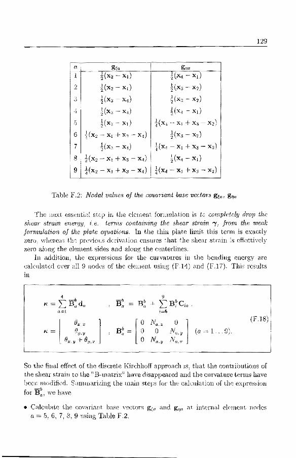
n g,. 'ff---~,-( X-2=--X~,)~

2

3

4

.5

6

ï

!g

Hx2 - x,)

~(X3 - X4)

!(x" x4 )

4(x2 X1)

~(x2 -x1 +x:.-x4 )

~(X3 - X4)

Hxz Xt + x,1 x 4) 1

l • ) 2 \X:i -· X2.

l(x, - X2)

lrx" - x,)

Hx, - x, + x:i - x2)

4(x3 x2 )

}(x1 - x 1 + X3 - x,j

l(x, - xi)

Ta.hle :F.2: Nodal valnes of 1.he co1;ar1.ant base vectors gt:a~ gtJa

129

The next. esseutiiîl step in t.lie element formnlation is to completcly drop l.hc .shcar stra·in ene1:<JY: (e. terïns coritairn.ri.g the shear stm:rn 1~ frorn the ?nenk fonnulation of the pla.te equat:ions. In t.he Uiin plate limit. t.his term is exact.ly zero: \Vhercas t.he previous derivnJ,]on ensurC'S that t)1e shcar strain is effer:tivcly :9ero a1ong r.he elctnent. sîdes and aloug the centerlines.

ln n.ddition, the expressions for the curvatures 111 the bcndiug encrg:J' are cakulatcd over all 9 nodes of the element. using (F.14) and (F.17). This results in

9

B~ + LB~Cio ~ t=f; i

0 (F 18'' " - J !

(a 1. .. 9).

So the fiual effect. of the discrete Kirchlwff approach is, t.hat the contributions of the shenr st.raiu to the'\ B-1natrix;; hHve disappenred and the curvaturc tcrrns have been modified. Suminarizing the main steps for the cakulation of the expression

-b for B 0 : \\'e ha.ve

• Calcnlate the covarînnt ba.se vectors gçn iu1d g,111 at înternal ele1nent no<lcs n ,, 5, 6, ï, 8, 9 using Tahle F.2.

130 APPENDIX F. A THIN DISCRETE KlRCHHOFF PLATE ELEMENT

• C3]culate the contravariant base veetors g~ and g~ at. the center node a = 9 b,v !llCitllS of (F. 7).

• Buik! t.be constraint mal.rice; C;0 of (F.14) and (F.17) for the mirlsicle a11d cent.er nocles.

• Finally: at. a given i11t.egrati~11 point., cnlcnlat.e t.be 111atrices J3! fro1n (F.18).

To .:.:heek the correcr.nf'..ss of the discrete ){irchhoff strategy adopLed in this ap­pendix~ r.he c}e111c11t is nscd in !5'.01ne silnple t.est ca..;;es.

Test case 1 (Cantilevered plate). In the first, cxample we consider a cantilevercd plal.e. The plate bas lengl:h t 10 n1n1: \\'idth b l n1n1 and thickncss d OJ 111111. The e1nstic pa.ra1netcrs here are E,. = E, = 1000 N/rnm2 and v, = "v = 0. One end of r.he plate a.t :c = 0 is clamped (nodes 1 aJJd 8), where;~s the othcr end (nodcs 7 and 14) is loadecl by elther a u11iforn1ly tra11s\:erse force Po or a, uniforn1ly dlstributed bending n101nent M0 . The specific element nwsh used in this calculntion is plot.ted in Fig F.2. The pln.t.e is divîded in G dist.orte<l e]e111cnt~: iH orrlcr to ~ho\v t.he insensit.lvi ty of the solution to n1esh dist.ort.ions.

If the plate is loaded by a bending momem m. r.he tip, the exact solut.ion yields a constant hending moment M" = M0 throughout the pla.te. lf the t.ip .Joad is n. transverse force, the bending n10111ent n1ust. var:y linea.rly nlong the phtt.o in 1>direct.Jon, i.e. M". = P0 (f - x). A linem· moment distribut;ion is only possihle, beca11se of the q1rndratic intcrpolation for the rolatious 00 in (F.4).

The present elen1ent. produces t.h~ correct a11S\Yers: '"hich can be secn in Fig F.3 whcre the value of M" in the intcgration points, nearest the lower eclgc y 0 has been plotied, toget.her with the exad solutiou.

•:node

B 9

2

-0.5~····-~,--

x : !ntegraUon point

MESH

10 11

4 5

4 6 :-: !mm]

6 7

6 10

Figure F.2: A patch of 6 distorted elements for u cantilevered plate, loadr.d at the tip by fa) o tmnsverse force and (b) a bcnding rnomcnt

131

normalized bending moment Mxx in integration points

2[ 1.8. case 1 : constant moment at tip

1.6 case 2 : constant transverse force at lip

1.4 e--··~ present element

1.2 exact solution ~

"~

-~. 0.2 0.4 0.6 0.8

xll

Figure F.3: Calculated bending moment Mxx in the lower row of integration points, for bath loading cases. The moment is normalized with its value at x 0

Test case 2 (Hinged cylindrical panel). The second exarnple is taken frorn a paper by Hughes and Liu [41] and it concerns a hinged cylindrical panel, loaded by a central point load. A cornparison with the calculation in [41] is only possible, because the shell equations in Chapter 4 have been set up fora cylinder, including geornetrically nonlinear effects.

e254o .§.

"2530

Hinged cylindrical panel under concentraled load

• Hughes-Liu

present study

2 4 6 center displacement [mm]

L=508 mm d=12.7mm E = 3103 Nlmm"2 nu= 0.3

8

MESH

y [mm] x [mm)

10

Figure F.4: Mesh and load-displacement plot fora hinged cylindrical panel

132 APPENDIX F. A THIN DISCRETE KIRCHHOFF PLATE ELEMENT

The cylindrical panel has a radius R 2540 mm, thickness d = 12. 7 mm and the length of both straight and curved sides is L 508 mm. Elastic parameters in this case are: = Ey 3103 N/mm2 and Vx = Vy 0.3. A point load Pis applied at the center of the plate in the negative z-direction, where the straight edges of the plate are hinged and immovable. The center of the plate is positioned at y, z) (0, 0, R). Since this problem is symmetrie with respect to the center lines, only one quarter has to be modelled. A mesh of 6 x 6 distorted elements has been used in this calculation.

The center displacement has been plotted versus the loacl Pin Fig F.4, for the present element and the Hughes-Liu element from [41]. A good correspondence between both calculations can be observed, up to the buckling load of the panel.

133

List of symbols

Notation The following general notation is used to distinguish between vectors and columns, tensors and matrices, and their components.

tensor matrix components

T T T;i

vector column components

x x Xi

Tlms, each of the following lines contains equivalent expressions

r ' T·n = t = Tn ti = T;i ni .

c = A·B : c = AB C;i A;k Bki.

c = x·y c = XTY c X; Yi

T = C: E ' ~·· C;ikl Ek1. t}

Here we use the summation convention, that is automatic summation over re­peated indices, where Latin indices (i, j, k, or I, J, K, etc) take on the values 1, 2, 3 and Greek indices (a, /3, "(, etc) have the values 1, 2.

Roman symbols a

aaf3 A,B,C,F A da, dÄ b b; ba.8 Bi, B2, etc B1a, B2a: etc c

length of wrapped region metric tensor of shell middle surface operators in a weak formulation global matrix corresponding with A area element tape width volume force curvature tensor of shell middle surface B-matrices (containing shape functions and derivatives) nodal partitions of B-matrices leak factor in averaged Reynolds equation

134

Co:fJ Ga c, CKL

c 0(n) d d, da D, D 1, D 2 etc Dt, Db, D8

D~lh8' D~ih15 Dij, dij

e, e0tfJ E, Ei1

Ex, ê1, ê2, f; Fo:

j\;ft

F, F;K

G Gxy, Gxz, Gyz h, hd hrnin

H H 1(0) J k1 Kn f Lz(O) 1Va , 1Va, x , ,"!Va, y

ni, N; ~ l\f n,H

1Ve1i Nnd

N, No:.B Af, l'vfa/3

p,ji

Pc Pa q, qa

Q, Q°' R, Rd

third fundamental tensor of shell middle surface resultant applied couple per unit area right Cauchy Green tensor and components space of continous functions on n tape thickness column vector with (nodal) unknows ( material) coefficient matrices tape tensile, bending and shear stiffness (isotropic)

tape tensile, shear and bending stiffnesses ( orthotropic) deformation rates and deviatoric deformation rates membrane strains Lagrange strain tensor and components Young modulus base vectors applied body force resultant applied force per unit area total applied tape force and moment deformation gradient and components region in JR3

, or shear modulus shear modulus air film thickness, drum geometry foundation thickness, minimum film thickness characteristic film thickness first order Sobolev space on n Jacobian ( = det F) foundation stiffness Knudsen number Àa/ H) tape length space of square integrable functions on n shape function and derivatives for node a unit normal vector components unit normal vectors number of elements, number of global nodes membrane forces per unit length bending moments per unit length air pressure contact pressure ambient pressure lubricant flow transverse shear forces per unit length radius, drum radius

t' f::.t t*

i

t T T, tij u, v, w Ui, Vi

'11, v uo Uh

G' 0:

U, U°' u, ue x,y, z

X, iJ, X

Greek symbols Cl:

f3 Af) Îal 'Y r, ro, ru etc t5 6A, bB, etc bij, 6af3 t::. T/

e K,, Ka(3, K,

Àa

IJ, lJx, l/y

w

fl, flo p, Pd, Po Ç, Tj, ç Çi u B, Ba, 9

time, time step boundary stress stress vector uniform applied tape tension stress tensor and components in 3D displacement components or velocity components displacement components or velocity components displacement vectors hearing wall velocity components drum velocity components column with all (element) degrees of freedom coordinates position vectors

of wrap helix angle shear strains boundary in JR1

) JR2 or /El3

variational operator first variations Kronecker delta increment air viscosity small number strain column vector curvatures ambient molecular free path length Poisson ratio angular velocity region in /El1

' JR2 or /El3

mass density coordinates in parent element region normal coordinates in the space occupied by a shell stress column vector rotations

135

Generally, barred quantities (u, p, d, etc) denote vveight functions, whereas quan-tities with an asterisk (u~, etc) denote prescribed boundary values. A sub-script 0 (p0 , w0 , etc) is used initial values, whereas a superscript e , we, etc) is used for a quantity a.ssociated with the e-th element. A subscript n (pn, wn, etc) is used to denote a quantity at time tn. A comma in a subscript always

136

denotes differentiation with respect to the quantity following the comma, e.g.

( ... ),x 8 ... 8x

( ... ) , °'

Calligraphic symbols t3 body 0 origin of coordinate system P point

P,

u,v, w u,v,w 8, 8x, 8y

8, 8x, 8y

s,s

pressure trial and weight function space

displacement trial function spaces

displacement weight function spaces

rotation trial function spaces

rotation weight function spaces

trial and weight function product space

[) ...

ÖXa

sh sh l finite dimensional trial and weight function space

Abbreviations DMV Donnell Mushtari Vlasov FEM Finite Element Method FDM Finite Difference Method RM Reissner Mindlin VHS Video Home System VCR Video Cassette Recorder lD One-Dirnensional 2D Two-Dimensional 3D Three-Dirnensional

137

References

[1] ADAMS, J., ET.AL. The Fortran 90 Handbook - Complete ANSI/ISO Reference. McGraw Hill Book Company, New York, 1992.

[2] ALBRECHT, D., LAENEN, AND LIN, C. Experiments on the Dynamic Re-sponse of a Flexible Strip to Moving Loads. IBM J. Res. Dev. 21 (1977), 379-383.

[3] ALLAIRE, P., AND BENSON, R. A Rapid Solution Method for the Compressible Reynolds Equation in Magnetic Recording Applications. Jlrib. Mech. Magn. Star. Syst. 4, STLE SP-22 (1987), 33-39.

[4] BATHE, K., AND DVORKIN, E. Short Communication A Four-Node Plate Bend­ing Element Based on Mindlin Reissner Plate Theory and a Mixed Interpolation. Int. J. Num. Meth. Eng. 21 (1985), 367-383.

[5] BAUMEISTER, H. Nominal Clearance of the Foil Bearing. IBM J. Res. Dev. 7, 2 (1963), 153-154.

[6] BELYTSCHKO, T., AND HUGHES, T. Computational Methods for Transient Anal­ysis. North-Holland, 1983.

[7] BENSON, R. Plate Tenting With a One-Sided Constraint. Trans. ASME J. Appl. Mech. 58 (1991), 484-492.

[8] BENSON, R., BREWEN, A., AND PIARULLI, V. A Simple Procedure for Deter­mining Elastohydrodynarnic Equilibrium and Stability of a Flexible Tape Flying over a Recording Head. Jlrib. Mech. Magn. Star. Syst. 2, STLE SP-19 (1985), 43-51.

[9] BENSON, R., AND SuNDARAM, R. A Green's Function with Improved Conver­gence for Cylindrically Wrapped Tapes. Trib. Mech. Magn. Star. Syst. 6, STLE SP-26 (1989), 98-110.

[10] BHUSHAN, B. Tribology and Mechanics of Magnetic Storage Systems. Springer Verlag, New York, 1990.

[11] BLOK, H., AND VAN ROSSUM, J. Foil Bearing A New Departure in Hydrody­namic Lubrication. Lubrication Engineering 9, 6 (1953), 316-320.

[12] BoGY, D., GREENBERG, H., AND TALKE, F. Steady Solution for Circumferen­tially Moving Loads on Cylindrical Shells. IBM J. Res. Dev. 18 (1974), 395-400.

138 REFERENCES

[13] BROESE VAN GROENOU, A., FIJNVANDRAAT, J., KADIJK, 8., AND VERBUNT, J. The Shape of Heads for Tape Recording: Experiments and Calculations for Various Trib. Mech. Magn. Star. Syst. 6, STLE SP-26 {1989), 120-127.

[14] BROESE VAN GROENOU, A., AND MEULENBROEKS, H. On the Laws of Head \Vear in Video Tape Recording - The lnfluence of Pressure and Time. Trib. A1ech. Magn. Star. Syst. 5, STLE SP-25 (1988), 108-116.

[15] CRISFIELD, M. A Four Noded Thin Plate Bending Element using Shear Con­straints a Modified version of Lyons Element. Comp. Meth. Appl. Mech. Eng. 38 (1983)' 93-120.

[16] DE WITH, P., RIJCKAERT, A" KEESEN, H., J., AND OPELT, C. An Experimental Digital Consumer HDTV Recorder using MC-DCT Video Compres­sion. IEEE Trans. on Consumer Electronics 39, 4 (1993), 711-722.

[17] D1x, G. Video, Dat Zit Zo. Zorn Uitgeverij B.V 1983.

[18] ERINGEN, A. Mechanics of Continua. John Wiley and Sons, Ine" 1967.

[19] ERINGEN, A. Continm1m Physics - Continuurn Mechanics of Single Substance Bodies, vol. 2. Academie Press, 1975.

[20] ERINGEN, A., AND SUHUBI, E. Elastodynamics, vol. 1. Academie Press, 1974.

[21] ESHEL, A. Compressibifüy Effects on the Infinitely Wide, Perfectly Flexible Foil Bearing. Trans. ASME J. Lubr. Tech. 90 (1968), 221-225.

[22] EsHEL, A. The Propagation of Disturbances in the Infinitely Wide Foil Bearing. Trans. ASME J. Lubr. Tech. 91 (1969), 120-125.

[23] ESHEL, A. On Fluid Inertia Effects in Infinitely Wide Foil J. Lubr. Tech. (1970), 490-494.

Trans. ASME

[24] ESHEL, A. Reduction of Air Films in Magnetic Recording by External Air Pres­sure. Trans. ASME J. Lnbr. Tech. 15 (1974), 247-249.

[25] A., AND ELROD, H. The Theory of the Infinitely Wide, Perfectly Flexible, Self-Acting Foil Hearing. Trans. ASME J. Basic Eng. 87 (1965), 831-836.

[26] ESHEL, A., AND ELROD, H. Stiffness Effects on the Infinitely Wide Foil Bearing. Trans. ASME J. Lnbr. Tech. 89 (1967), 92-97.

A., AND \VILDMAN, M. Dynamic Behaviour of a Foil Bearing in the Présence of a Lubricating Film. Trans. ASME J. Appl. Mech. 35 (1968), 120-125.

[28] N., AND TALKE, F. Capacitance Probe Study of Rotating-Head/Tape Interface. IBM J. Res. Dev. 21 (1977), 289 293.

Theory and Fluid Pilrn Lubrication Leeds Lyon Osborne Reynolds Centenary

(1987), 539 542.

REFERENCES 139

[30] FLÜGGE, W. Stresses in Shells. Springer-Verlag, 1973.

[31] G.D. GRANZOW AND A.0. LEBECK. An improved one-dimensional foil hearing solution. Trib. Mech. Magn. Stor. Syst. 1, STLE SP-19 (1984), 54-58.

[32] GILBERT, J., MOLER, C., AND SCHREIBER, R. Sparse Matrices in Matlab: Design and Implementation. SIAM J. Matrix Anal. Appl. 13, 1 (1992), 357-385.

[33] GREEN, A., AND ZERNA, W. Theoretical Elasticity. Oxford University Press, 1954.

[34] GREENBERG, H. Study of Head-Tape Interaction in High Speed Rotating Head Recording. IBM J. Res. Dev. 23, 2 (1979), 197 205.

[35] GROSS, W. Fluid Film Lubrication. John Wiley and Bons, Ine., 1980.

(36] HACKBUSCH, W. Multi-Orid Methods and Applications, vol. 4 of Springer Series in Computational Mathematics. Springer-Verlag, 1980.

[37] HEINRICH, J., AND CONNOLLY, D. Three-Dimensional Finite Element Analysis of Self-Acting Foil Bearings. Comp. Meth. in Appl. Mech. and Eng. 100 (1992), 31-43.

[38] HEINRICH, J., AND WAHDWA, S. Analysis of Self-Acting Foil Bearings: A Finite Element Approach. Trib. Mech. Magn. Stor. Syst. 3, STLE SP-21(1986),152-159.

[39] HUGHES, T.J.R. The Finite Element Method. Prentice-Hall International, 1987.

[40] HUGHES, T., AND BREZZI, F. On Drilling Degrees of Freedom. Comp. Meth. Appl. Mech. Eng. 72 (1989), 105-121.

[41] HUGHES, T., AND LIU, W. Nonlinear Finite Element Analysis of Shells: Part I. Three Dimensional Shells. Comp. Meth. Appl. Mech. Eng. 26 (1981), 331-362.

[42] HUGHES, T" AND TEZDUYAR, T. Finite Elements Based Upün Mindlin Plate Theory with Particular Reference to the Four-Node Bilinear Isoparametric Ele­ment. Trans. ASME J. Appl. Mech. 48 (1981), 587-596.

[43] IBM. Engineering and Scientific Subroutine Library, Guide and Reference - Re­lease 4. IBM Corp., 1990.

[44] IBM. AIX XL Fortran Compiler/6000 Language Reference, Version 3, Release 1. IBM Corp., 1993.

[45] ITOH, J., EBIHARA, T., AND TAKAHASHI, A. Simulation of Tape Floating Be­haviour in VTR. ITEJ Techn. Rep. 15, 75 (1991), 19-24.

[46] JORGENSEN, F. The Complete Handbook of Magnetic Recording. TAB Books, Ine., 1980.

[47] KOITER, W. On the Nonlinear Theory of Thin elastic Shells. Proc. Kon. Acad. Wetensch. B 69 (1966), 1-54.

140 REFERENCES

[48] KOTERA, H., KITA, H., KAMINAKA, N" HIROSHI, Y., AND MIZOH, Y. Inter­changeability of VTR Tapes and its Computational Analysis. to be published in ASME, AISS (1991).

[49) KOTERA, H., KITA, H., KAMINAKA, N., YOHDA, H., AND MIZOH, Y. Analysis of Tape Floating Behaviour on Magnetic Head and Grooved Drum in VCR. ASME, Industr. and Env. Appl. of Fluid Mech. FED-Vol.145 (1992), 151-156.

[50) KOTERA, H., KITA, H., MIZOH, Y., AND YOHDA, H. Finite Element Analy­sis of the Interface Phenomena between VCR Tape and Head. IEEE Trans. on Consumer Electronics 37, 3 (1991), 224-227.

[51] KOTERA, H" KITA, H" MIZOH, Y., AND YOHDA, H. Head Wear and Repro­duction Envelope Simulation by FEM. Magnetic Recording 63 (1991), 53-58.

(52) KOTERA, H., KITA, H., MIZOH, Y" AND YOHDA, H. Interchangeability of VCR Tapes and Head-Tape Interface Technology. National Tech. Rep. 37, 3 (1991), 128-135.

[53] KOTERA, H" KITA, H., MIZOH, Y., AND YOHDA, H. A New Scheme for Finite Element Analysis of an Interface Phenomena of VCR Drum Head and Tape. IEEE Tmns. on Consumer Electronics 38, 3 (1992), 181-187.

(54] KOTERA, H., KITA, H" MIZOH, Y., YOHDA, H" AND INOUE, K. Influence of Mechanica! Anisotropy of Magnetic Tape on Head to Tape Interface in VCR. J. Magn. Soc. Japan 15, 82 (1991), 709-714.

[55] LACEY, C., AND TALKE, F. Measurement and Simulation of Partial Contact at the Head/Tape Interface. Trans. ASME J. Trib. 114 (1992), 646-652.

[56] LANG LO IS, W. Statie Determinacy in the Theory of the Finite Width Foil Bearing. Trans. ASME J. Appl. Mech. 41 (1974), 51-54.

(57] LANGLOIS, W. Finite Width Foil Bearing with Light Loading. Tmns. ASME J. Appl. Mech. 42 (1975), 274-278.

[58] LANGLOIS, W. Iterative Solution of Finite Width Foil Hearing Problems. Comp. Meth. in Appl. Mech. and Eng. 14 (1978), 249-258.

[59] LEKHNITSKII, S. Anisotropic Plates. Gordon and Breach, Sc. Publ. Ine., 1968.

[60] LICHT, L. An Experimental Study of Elastohydrodynamic Lubrication of Foil Bearings. Trans. ASME J. Lubr. Tech. 90 (1968), 199-220.

[61] LUIT JENS, S. Magnetic Recording Trends: Media Developments and Future Video Recording Systems. IEEE Tmns. on Magn. 26, 1 (1990), 6-11.

[62] METCALF, M" AND REID, J. Fortran 90 Explained. Oxford University Press, 1990.

REFERENCES 141

[63] MITCHELL, A., AND GRIFFITHS, D. The Finite Difference Method in Partial Differential Equations. John Wiley and Sons, Ine., 1980.

[64] MITSUYA, Y. Modified Reynolds Equation for Ultra-Thin Gas Film Lubrication using 1.5-order Slip-Flow Model and Considering Surface Accomodation Coeffi­cient. Trans. ASME J. Trib. 115 (1993), 289-294.

[65] MITSUYA, Y., AND ÜKUBO, T. Averaged Reynolds Equation extended to Gas Lubrication Possessing Surface Roughness in the Slip Flow Regime. Trans. ASME J. Trib. 111 (1989), 495-503.

[66] MOES, H. Multi-Grid Calculations of the Air Gap between Tape and Drum in a Video Recorder. Presentation on the 2nd genera[ CAMST meeting, Enschede (1990).

[67] MÜFTÜ, S., AND BENSON, R. Numerical Simulation of Tape Dynamics in Helical­Scan Recording. to be published in IEEE Trans. on Magn. (1993).

[68] NAG. NAGWare f90 Compiler - The Essential. The Numerical Algorithms Group Ltd., 1992.

(69} NIORDSON, F. Shell Theory, vol. 29 of Series in Applied Mathematics and Me­chanics. North-Holland, 1985.

[70] ÜNO, H., ÜKAMATA, T., KAKU, N., ÜGIRO, K., ÜZAKI, s., AND SCOTT, F. A New Drum and Heads for the D-2 Digital VTR. SMPTE J. (1991), 596-600.

[71] PRATHAP, G., AND BHASHYAM, G. Reduced lntegration and the Shear-Flexible Beam Element. Int. J. Num. Meth. Eng. 18 (1982), 195-210.

[72] REID, J. The Advantages of Fortran 90. Computing. 48 (1992), 219-238.

[73] RONGEN, P. On Numeri cal Solutions of the Instationary 2D Foil Bearing Problem. Trib. Mech. Magn. Stor. Syst. 7, STLE SP-29 (1990), 130-138.

[7"1] SAKAI, K., TERAYAMA, T., MORIKAWA, J., AND ÜHWADA, N. Study of Head­Tape Interference in VCR's. JSME Int. J. 33, 4 (1990), 655662.

[75] SAKAI, K., TERAYAMA, T., ÜKAMOTO, N., AND TAMURA, T. Contact Anal­ysis Between Magnetic Heads and Magnetic Tapes of Video Cassette Recorder -Analysis with Infinite Width Heads. JSME Int. J. 31, 2 (1988), 188-195.

[76] SAKAI, K" TERAYAMA, T., ÜKAMOTO, N., AND YOKOTA, H. Clearance Char­acteristics between Magnetic Tapes and Heads of Video Cassette Recorders. Trib. Mech. Magn. Star. Syst. 4, STLE SP-22 (1987), 61-67.

[77] SANDERS, J. Nonlinear Theories for thin Shells. Q. Appl. Math. 21, 1 (1963), 21~36.

[78] SCHLICHTING, H. Boimdary Layer Theory. McGraw-Hill, New York, 1968.

142 REFERENCES

[79] SHAKIB, F., HUGHES, T., AND JOHAN, Z. A Multi-Element Group Preeondi­tioned GMRES Algorithm for Nonsymmetrie Systems Arising in Finite Element Analysis. Comp. Meth. Appl. Mech. Eng. 75 (1989), 415-456.

[80] SMITH, D., AND VON BEHREN, R. Squeeze Film Analysis of Tape Winding Effeets in Data Cartridge. Trib. Mech. Magn. Stor. Syst. 6, STLE SP-26 (1989), 88-92.

[81] STAHL, K., WHITE, J., AND DECKERT, K. Dynamie Response of Self-Acting Foil Hearings. IBM J. Res. Dev. 18 (1974), 513-520.

[82J STOLARSKY, H., AND BELYTSCHKO, T. Shear and Membrane Loeking in Curved c0 Elements. Comp. Meth. in Appl. Mech. and Eng. 41 (1983), 279-296.

[83] TANI, T., SHIMEGI, H., AND MIWA, H. On the Behaviour of Magnetic Tape in Self-Acting Foil Bearings. Trib. Mech. Magn. Stor. Syst. 4, STLE SP-22 (1987), 5460.

[84) TANNER, R. Engineering Rheology. Clarendon Press, Oxford, 1985.

[85] THE MATHWORKS INC. MATLAB User's Guide. The MathWorks Ine., 1992.

[86] TIMOSHENKO, S., AND GERE, J. Mechanics of Materials. Van Nostrand Reinhold Comp., 1973.

[87] TIMOSHENKO, AND WOINOWSKY-KRIEGER, S. Theory of Plates and Shells, 2nd ed. MeGraw-Hill, 1959.

[88] TROUTMAN, J. Variational Calculus with Elementary Convexity. Springer-Verlag, New York, 1983.

[89) UENAKA, H., MUKAE, H., A.KUROE, AND MIKODA, M. Relationship between Head/Tape Contact Conditions and Tape Stiffness. IEEE Trans. J. Magn. Jap. 5, 2 (1990), 142 147.

[90] WALOWIT, .J., AND ANNO, J. Modern Developments in L1tbrication Mechanics. Applied Scienee Publishers Ltd., London, 1975.

[91] WOLF, B., DESHPANDE, N., AND CASTELLI, V. The Flight of a Flexible Tape Over a Cylinder with a Protruding Bump. Trans. ASME J. Lubr. Tech. 105 (1983), 138-142.

[92] YONEDA, K" AND SAWADA, T. Simulation of Spacing between Magnetic Head and Medium of Video Floppy. IEEE Trans. J. Magn. Jap. 2, 6 (1987), 490-496.

[93] YONEDA, K., AND SAWADA, T. Simulation of Tape Flying Characteristies Above VTR Drum Considering In-Plane Stress. IEEE Trans. J. Magn. Jap. 4, 2 (1989), 128-134.

[94] YoNEDA, K., AND SAWADA, T. Simulation of Tape Glide Characteristics Above VCR Drum with Rotating Part and Statie Part. IEEE Trans. J. Magn. Jap. 4, 11 (1989), 717-727.

REFERENCES 143

[95] ZIENKIEWICZ, 0., AND TAYLOR, R. The Finite Element Method - Basic Formu­lation and Linear Problems, 4th ed., vol. 1. Mc-Graw Hill, 1989.

(96] ZIENKIEWICZ, 0., AND TAYLOR, R. The Finite Element Method Solid and Fluid Mechanics Dynamics and Non-Linearity, 4th ed., vol. 2. Mc-Graw Hill, 1991.

18 februari 1960 :

1972-1978

1978-1986

1986-1988

1988-heden

In English:

Curriculum Vitae

geboren te Heerlen.

Bernardinus College te Heerlen, diploma Atheneum B in 1978.

Technische Universiteit Eindhoven, afdeling Technische Natuurkunde (1978-1979) afdeling Wiskunde en Informatica (1979-1986) (afgestudeerd in de vakgroep toegepaste analyse, o.l.v. Dr. Ir. A.A.F. van de Ven).

wetenschappelijk medewerker bij het Natuurkundig Laboratorium van Philips, groep "Displays and Cathodes", o.l.v. Dr. W.M. van Alphen.

wetenschappelijk medewerker bij het Natuurkundig Laboratorium van Philips, groep "Applied Mechanics", o.l.v. Ir. B. Sastra.

The author of this thesis was bom in 1960 in Heerlen, The Netherlands, where he received his secondary education at Bernardinus College from 1972 to 1978. From 1978 to 1986 he studied at the Eindhoven University of Technology, initially in the faculty of Applied Physics and from 1979 in the faculty of Mathematics and Computer Science. In 1986 he received his engineering degree in mathematics (thesis on the analysis of magneto-elastic buckling of superconducting structures). In 1986 he joined Philips Research Laboratories as a member of the "Displays and Cathodes" department of Dr. W.M. van Alphen, where he worked on numer­ical methods for application within electron opties. From 1988 until now, he is working in the" Applied Mechanics" department of Ir. B. Sastra on the subject presented in this thesis.

Acknowledgments

The results of the research presented in this thesis, would have been unthinkable without the commitment, support and encouragement of many of the people in my daily environment. The following persons should be mentioned here :

The 'men of the very beginning': Jaap Fijnvandraat, Rob Boereboom, and Coen Warmenhoven who taught me my first steps in the world of magnetic record­ing.

My other colleagues in the magnetic recording area: Ben van Bakel, Guus Braun, Gerard van Engelen, Nol Broese van Groenou, Peter van Hoogstraten, Thijs de Jongh, Ad van Kasteren, Adri Keppel, Steven Luitjens, Anton Maas, Albert Rijckaert, Casper Smit, Marty van de Ven and Joost Wolf.

Frank Baaijens, Joost Horsten, Jurgen Rusch, 'Willem Potze and Jos van Vroonhoven for their valuable help concerning the theoretica!/ computational me­chanics problems, as well as the scientific programming.

My colleagues in the computer support department: Ad Leeuwestein, Arjan van Ham, Ronald van Rijn and Ed Reniers.

Peter Holster, Leo Tielemans, Jack van der Sanden, Ron Beerens and Jos van Vroonhoven, with whom I had many stimulating 'discussions' during lunch time. And all other group members, because each of them contributed significantly to the unique atmosphere in our department.

But above all my wife, because without her support this thesis would proba­bly never have been written.

Finally, I want to thank the management of the Philips Research Laboratory in Eindhoven, especially Ir. B. Sastra and Dr. G.E. Thomas, who allowed me to write a PhD thesis on my research work. This is also true for my former department leader, Prof. E.A. Muijderman, who actually initiated the work in this thesis.

Stellingen

behorende bij het proefschrift "Finite Element Analysis of the Tape Scanner Interface

in Helical Scan Recording" van P. M. J. Rongen

1. Bij toepassing van een niet-lineaire Gauss-Seidel techniek op het folielagerrnodel, levert een groepering van de onbekenden naar knooppunt en een relaxatievolgorde in stroomafwaartse richting, het betrouwbaarste iteratieschema.

Rongen, P.M.J" "On Numerical Soluti~ns of the Instationary 2D Foil Bearing Pro­

blem", Trib. Mech. Magn. Stor. Syst. 1, STLE SP-29 (1990), 130-138.

2. Voor berekeningen aan band-scanner en band-kop contactsituaties is het gebruik van een dun schaalelement gebaseerd op een discrete Kirchhoff techniek, beter dan een dik schaalelement gebaseerd op onafhankelijke interpolatie van de afschuifrek (bijv. "Tl element"). Het laatste type element vertoont onder omstandigheden contactdrukoscillaties in het contactgebied.

Dit proefschrift, hoofdstuk 4.

3. Heinrich en Conolly berekenen een stationaire oplossing voor het folielager via een instationair model dat rekening houdt met de massatraagheicl van de tape. Dit in combinatie met het door hun gebruikte algoritme, vormt een uiterst inefficiënte manier om genoemd probleem numeriek op te lossen. De maximaal toelaatbare tijdstap in het algoritme is veel te klein.

Heinrich J" and Conolly, D" "Three-Dimensional Finite Element Analysis of Self­

Acting Foil Bearings". Comp. Meth. Appl. Mech. Eng. 100, (1992), 31-43.

Dit proefschrift, hoofdstuk 3 en 5.

4. Het volledig gekoppeld oplossen van de elasticiteitsvergelijkingen en de Reynolds­vergelijking in het folielagerprobleem, resulteert in een betrouwbaarder algoritme dan dat waarbij deze twee vergelijkingenstelsels iteratief, om en om worden opgelost (Picard methode).

Dit proe!Schrift, hoofdstuk 3 en 4.

5. Door grote industriële belangen en hevige concurrentie op het gebied van magne~ tische recording is er een gebrek aan openheid in de wetenschappelijke literatuur hierover. Dit staat de oplossing van fundamentele vraagstukken op dit gebied in de weg.

6. Het ouderwetse imago van de FORTRAN programmeertaal is met de introductie van de nieuwe ISO Fortran-90 standaard duidelijk achterhaald. Algemene acceptatie van deze taal zal echter nog de nodige tijd vergen zolang de beschikbare compilers onbetrouwbaar blijken te zijn.

Reid, J., "The Advantages of Fortran 90", Computing 48, (1992), 219-238.

7. Multi-roostermethoden kunnen zeer efficiënt zijn, maar de probleemspecifieke aan­pak die niet zelden nodig is om de best mogelijke convergentiesnelheid te verkrijgen, heeft een negatieve invloed op de algemene toepasbaarheid van deze numerieke tech­niek.

8. Het ontbreken van een algemeen, gecombineerd schaal-smeerfilm element is een dui­delijke tekortkoming in commercieel verkrijgbare eindige elementen pakketten.

9. Het grote vertrouwen van niet-ingewijden in de voorspellende waarde van de eindige elementen methode bij toepassing op complexe, technische, industriële problemen, is onterecht.

10. Sommige politieke leiders wekken met het gebruik van een gekleurde politieke ter­minologie als 'paars kabinet' de indruk dat politieke ideologiëen additief mengbaar zijn, terwijl deze in werkelijkheid slechts subtractief mengbaar zijn.

11. Een user-accounting systeem waarbij rekentijd- en geheugengebruik worden omge­rekend in geld, als optie bij een gecentraliseerde computerondersteuning, kan alleen efficiënt zijn indien budgetoverschrijding directe financiële consequenties heeft voor de verantwoordelijke systeemgebruikers. Het aanbrengen van muntenapparaten op computerterminals kan in deze een eerste aanzet zijn.