JOURNAL OF MATHEMATICAL ANALYSIS AND APPLICATIONS 165, 180-191 (1992)

Finite Element Methods for Nonlinear Sobolev Equations with Nonlinear Boundary Conditions

Y ANPING LIN *

Department of Applied Mathematics, University of Waterloo, Waterloo, Ontario, Canada N2L 3GI

AND

TIE ZHANG

Departrnenr of Mathematics, Northeast University of Technology, Shenyang, People’s Republic of China

Submitted by Avner Friedman

Received February 6, 1990

We derive optimal L* error estimates for semi-discrete finite element methods for nonlinear Sobolev equations with nonlinear boundary conditions. A new projection is introduced and used in the error analysis. q> 1992 Academic Press, Inc.

1. INTRODUCTION

Let Q c Rd (d > 1) be an open bounded domain with smooth boundary X2. We consider finite element approximation to the solution of the following Sobolev equations:

c(u)u,-v. {a(u)Vu,+b(u)Vu} =f(u), in QxJ,

a(u) ~ + b(u) $ = g(u), ap

on LX2xJ, (1.1)

u( ‘) 0) = u, on Szx (O},

where J= (0, T), T>O, a, b, c, f, g, and v are known functions; P = (PI > . ..T ,DJ denotes the outer-normal direction on X2. We also assume that the functions a, b, c, f, and g are smooth with bounded derivatives and there exists C,>O such that

0 < co < a(u), C(U)? UER.

* Present address: Department of Mathematics, University of Alberta, Edmonton, Alberta, Canada T6G 2Gl.

180 0022-247X/92 $3.00 Copynght c 1992 by Academic Press, Inc. All rights ol reproduction in any form reserved

FINITE ELEMENT FOR SOBOLEV EQUATIONS 181

The problem (1.1) can arise from many physical processes. For the ques- tions of existence, uniqueness, and continuous dependence of the solutions and their applications, we refer to [2, 73 for extensive literature. For the numerical solution to Dirichlet boundary conditions, both finite difference and finite element methods have been studied by Ewing [S, 61, Ford [S], Ford and Ting [9, lo], and Wahlbin [15]. For problem (1.1) when g = g(x, t) and d < 3, finite element methods with time-stepping have been investigated by Ewing [7]. In these papers the authors obtained quasi- optimal L* error estimates except that of [ 151. While, Arnold, Douglas, and Thomee [ 1 ] and Nakao [ 121 considered finite element methods to a problem similar to (1.1) for d = 1 with periodic boundary conditions, they demonstrated some optimal error estimates and superconvergences. Some further investigations of finite element methods for Sobolev and other related type equations with homogeneous boundary data have been carried out by Lin, Thomee, and Wahlbin [ 111.

In this paper we study finite element approximation to the solution of (1.1) and show that the finite element solution uh indeed possesses an optimal order convergence rate to the real solution u as expected. In addi- tion, our results are valid for any space dimension d 3 1 provided that u, U, E H”(Q) with s > d/2 + 1. It is well known that the restriction on d< 3 for parabolic equations [4] and Sobolev equations [7] cannot be removed because of the nonlinearity of the boundary data and the method used there. Hence, our method, at this point, has some advantages and provides, at least, some theoretical significances into the literature.

Let H”(Q) and H”(X!) be Sobolev spaces of order s with norms II.II s and ( .Is, and (., .) and (., .) denote the inner products in L*(Q) and L*(%2), respectively.

Let S, be a family of finite dimensional subspaces of H’(Q) such that for some r 2 2.

inf (lb-xll +~ll~-~Il~~~~~“Il~ll,~ 1 <s<r, u~ff”(Q). XS&

We also assume that Sh is imposed on quasi-uniform triangulation of s2 such that the usual inverse inequalities hold [3, 71.

The semi-discrete finite element solution uh: J-+ S,, is now defined by

(C(%) Uh,!, xl + (4uh)vuh.t + WUh)VUh, Vx)

= (fz(Uh), x > + u-(u,h XL XESh

uh(“) = uh

(1.2)

where v,, is an appropriate approximation of v into S,. Now let us state our main theorem in this paper.

182 LIN AND ZHANG

THEOREM. Let u and u,, be the solutions of (1.1) and ( 1.2), respectively, u, Vu, uI, artd Vu, are bounded, and 1.4, u, E H”(Q) with s > d/2 + 1. Then there exists C= C(u) > 0, dependent upon the norms of the solution u mentioned above, such that

Ilu(t) - ~Jf)ll + IIu,(t) - +,,(t)ll d C(u) h”> (1.3)

provided that v E H”(Q) and oh is given by

(v~v-~,),vx)+(~--uh,x)=o, XESh. (1.4)

In next sections we shall use the following inequalities:

AB Q &A2 + B2/4&, E > 0, (1.5)

l4:2(m2 ~~11~~112+~~~~11~112, E > 0, (1.6)

I~Ir~Ci-,rl14r+l,2~ O<r<i,r#l. (1.7)

In Section 2 we introduce a new projection W and study its approxima- tion properties. The proof of the theorem will be given in Section 3.

2. A NEW PROJECTION W(t)

In order to derive optimal error estimates for finite element approxima- tions for diffusion type problems, it is well known [ 14, 161 that it is necessary to introduce Ritz projection into the analysis. The authors of [l, 7, 8, 12, 151 took this standard approach to treat the problems considered therein.

As a preparation of the proof for the theorem stated in Section 1, instead of using Ritz projection, we shall introduce an auxiliary function, called nonlinear nonclassical elliptic projection of the solution u into finite element spaces S,, which is now defined in the following way: Let 13 0 and W(t): [0, T] -+ S, be defined by

(a(u) V( W, - u,) + b(u) V W- u), Vx) + 4 W, - u,, xl

-(g(w-du),x)=o~ t>o,XESh,

W(O)=v,ES~.

(2.1)

We see, of course, that the study of this new projection will certainly take some extra effort, but optimal error estimates can be demonstrated in a very simple way as usual for parabolic equations [4, 143 if this projection W(t) is used (see Section 3).

We show that W(t) in (2.1) is well defined.

FINITEELEMENT FOR SOBOLEV EQUATIONS 183

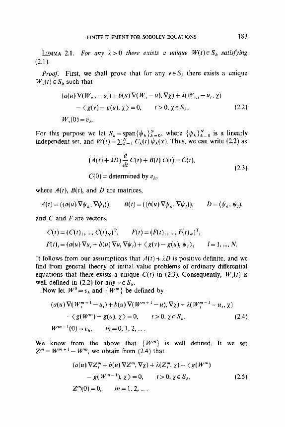
LEMMA 2.1. For any I > 0 there exists a unique W(t) E S,, satisfying (2.1).

Proof: First, we shall prove that for any v E S,, there exists a unique W,(t) E S,, such that

(a(u) V WV,, - u,) + b(u) V WV - u), Vx) + 4 W,,,, - 4, x)

- ( g(v) - g(u), x > = 0, t>o, XESh,

W,(O) = Uh.

(2.2)

For this purpose we let S,=span{$,},N=O, where ($,}f=, is a linearly independent set, and W(t) = Cp=, C,(t) $,Jx). Thus, we can write (2.2) as

(‘4(t)+io)-$C(t)+B(t)C(t)=C(t), (2.3)

C(0) = determined by oh,

where A(t), B(t), and D are matrices,

A(t) = ((a(u) Wk, Wd), B(t) = ((b(u) w/o W,)), D = (Ic/,o +A

and C and F are vectors,

C(t) = (C(t), 3 . . . . c(0,)‘, J’(t) = (F(t),, . . . . F(t),v)=,

F(t),= (a(u) Vu, + 4~) Vu, WJ + (g(v) - g(u), $,>, 1= 1, . . . . N.

It follows from our assumptions that A(t) + AD is positive definite, and we find from general theory of initial value problems of ordinary differential equations that there exists a unique C(t) in (2.3). Consequently, W,(t) is well defined in (2.2) for any v E S,,.

Now let W” = v,, and { Wm> be defined by

(a(u)V(Wy+’ - u,) + b(u) V( W” + ’ -U),VX)+E.(W’:-+‘-u,,X)

- (g(W”)- g(u), x> =o, t>o,XESh, (2.4)

wm+‘(o) = Uh, m=0,1,2 )....

We know from the above that { Wm} is well defined. It we set Z”= wm+l - W”, we obtain from (2.4) that

(a(u) VZY + b(u) VZ”, W + WY, xl - (A WY

-g(W”-‘),x)=0, t>o,XESh, (2.5)

Zrn(0) = 0, m = 1, 2, . . .

184 LIN AND ZHANG

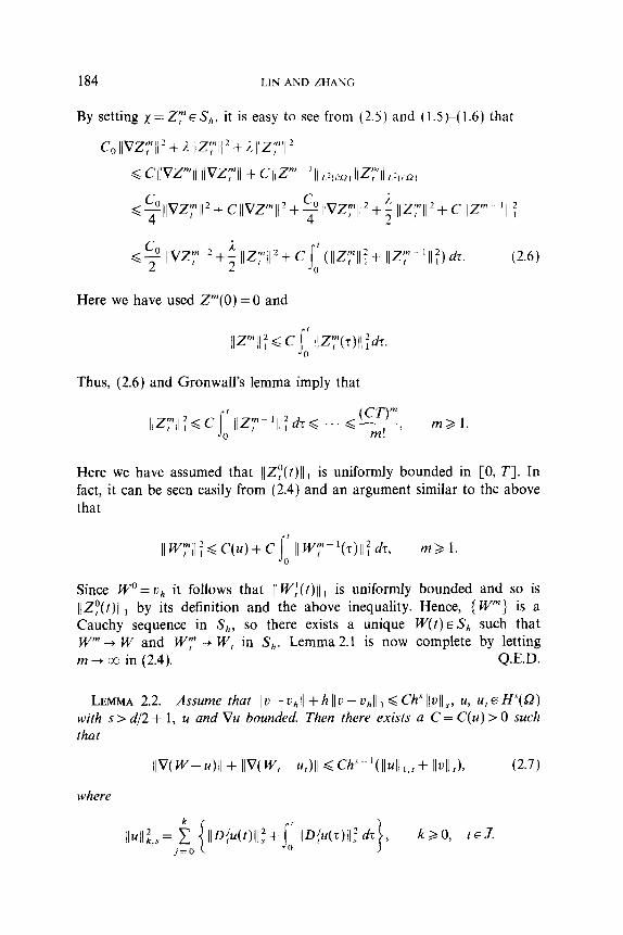
By setting x= .Z~ES~, it is easy to see from (2.5) and (1.5)-( 1.6) that

co llvz;~ll z + 1 llZ’:ll 2 + J. llZyql 2

d ~lIVZ”ll IIVZ~II + CIIZ”’ %‘(r’R, llm1.&Y2l

~~llvz:“ll’+cIIvz”l,‘+~llvz:‘l/‘+~ /lz:“l~2+cIlz” ‘11:

<$ Ilvzy +; llZy”+ CI; (llz’;1ll:+ IIZT ‘II:, dz. (2.6) 0

Here we have used Zm(0) = 0 and

Thus, (2.6) and Gronwall’s lemma imply that

Here we have assumed that IlZf(t)ll , is uniformly bounded in [0, r]. In fact, it can be seen easily from (2.4) and an argument similar to the above that

Since W” = oh it follows that (( W:(t)11 r is uniformly bounded and so is IlZ~(t)ll r by its definition and the above inequality. Hence, { Wm} is a Cauchy sequence in S,, so there exists a unique W(t) E Sh such that W” + W and WY -+ W, in Sh. Lemma 2.1 is now complete by letting m -+ co in (2.4). Q.E.D.

LEMMA 2.2. Assume that /lu-z~~)l +hllv--uhlll ~Ch~lluil,, u, u,EH”(Q) with s > d/2 + 1, u and Vu bounded. Then there exists a C = C(u) > 0 such that

Ilv(W-u)/l + IlV(W,-u,)ll < Chs~-‘(IIull,..~+ Ilulls), (2.7)

where

FINITE ELEMENT FOR SOBOLEV EQUATIONS 185

Proof: Let q = W-U and P,: L*(a) + S, be L* projection [3, 141. We know from (2.1), (1.5t(1.7), and [3, 141 that

(a(u) VY, + b(u) V% VY,) + 4rl,, rlt) - (g(W) - g(u), rlt)

d (a(u) V?, + b(u) vrl, Ru - PhU),)

+4ilt, (u-phu),)- <g(W)-g(u), (u-phU)t)

d CW?,ll + IIWI) IIVU- PhU),)ll + CII?,II ll(~-P,~M

+ CIl’1IlLqan) Il(u- ph~),lILq,?Q)

and then,

+ ch2s-2 w41:+ Ilu,ll:)icjd IlvltllV~.

From Gronwall’s lemma and our assumptions on uh we obtain

IIPtll:d~~2”~2~ll~ll:,,+ ll4f,. (2.8 1

Hence, Lemma 2.2 follows from

ll~ll:~clls~o~ll:+c~~ IlIrlX~~. Q.E.D. (2.9)

We now turn to an estimate for q = W- u in L*(O).

LEMMA 2.3. Under assumptions of Lemma 2.2 and Iv - v,, ~ 1,2 < Ch”(lv(ls. We have

l/v/l + llrl~ll G CWll4 l,s+ ll~lld. (2.10)

Proof: Let cr~H’(S2) such that

(a(u)Vcr+b(u)Vq,VJ’)+I(cr, I’- (Gq, V)=O, VE H’(Q), (2.11)

186 LIN AND ZHANG

where

G=~ol~(eu+(l -e)W)de.

The existence and uniqueness of such x E H’(Q) is guaranteed by taking 1, large enough. We shall, from now on, assume that 2 is big enough (fixed) for all our needs. We see from (2.1) and (2.11) that

(a(u) vvl, - a), Vx) + 4v, - 4 x) = 0, XESh. (2.12)

Noticing that ~~-a= IV-u,--CI= W,- (~,+a), we see that W, is actually a standard Ritz projection of U, + CI into S,, so that we have from Lemma2.2 and [3, 14, 161,

IlW,--,--II d~~I/~,-~,-~ll,d~~~llrl,ll,+ Il4l,)

G CW4l,,+ lMJ+ CWll,. (2.13)

Also, we see that the elliptic regularity and (2.11) imply

II41 d CIIVrlIl + Cllrlll LWQ)~ Mill1 G Ch” ‘(ll4,,+ lI4I,), and hence,

llv,-~11 ~Ch”(ll41,,+ Ilull.,). (2.14)

It remains now to estimate /Iall. Let p E H’(Q) be defined by

(a(u) VP + b(u) Vr, W + W, v) - ((3, V = (a, I’), VE H’(S2). (2.15)

If we set V = c( in (2.15) and V = p in (2.11), we obtain from integration by parts, (1.5)(1.7), and our assumptions that

ll~l12=~~~~~~B+~~~~~rl,~~~+~~B,~~-~~rl,~~

=(Qu)Vv,Va-PI)- (Grl,a-B>

FINITE ELEMENT FOR SOBOLEV EQUATIONS 187

We obtain by subtracting (2.15) from (2.11) that

(a(u) V(a - P), w + 4a - 8, v = (4 0 VE H’(SZ),

and, thus, Ilcr-bljz< Cjlorll. It is now easy to see by taking E small (fixed) in (2.16) that

By (2.14) and (2.17) we See that we need to estimate lq,lP,,2. For this purpose we let yeH’(B) be such that

(a(u) YJ + b(u) Vv, W + 4~ V - (Grl, 0 = (4 J’>, VE H’(Q), (2.18)

where ~EH’/*(~Q) and 161,,2= lqtlLl,2, (6, q,>= lq121,2. Setting @ = y - tl, it follows from (2.11) and (2.18) that

(a(u) V@, VV) + A(@, V) = (6, V), VE H’(Q) (2.19)

and, then, the elliptic regularity implies

II~II2~~l~l~,*=~l?rl~1/2~ (2.20)

Now let V=qt in (2.19) together with integration by parts and (1.5)-( 1.7). We obtain

ld2,,2 = (a(u) V@> VI1t) + 4@, ?,I = (a(u) vv,, V@) + JOI,, @)

= (a(u) vv, + b(u) V?, V@P) + 4?,, @I

- (‘3, @> + <Grl, @> - (b(u) Vrl, V@)

= (a(u) vrlt + b(u) V% V(@ - Zh@))

+4rlr, @-I,@,)- <@I,@-I,@>

+(Gg,m)-(g,~h(u)Q)+(~,V.b(u)V~)

&?,ll:+ ll’111~~+~ll~ll:+~lr112112 E

+4I@--h@l:,2+ l@l1,2)+cll~ll ll@ll*

+~llull:;,+ llBli)+W@ll’:+~s,~ lv,l?1,2dr. (2.21)

188 LIN AND ZHANG

Taking E small (fixed), we find from (2.20) and (2.21) that

Applying Gronwall’s lemma to above inequality, we see

I~rlZ~~2d~~*“~Il~ll:.*+ Ildf). (2.22)

Using (2.22), (2.17), and (2.14) we see again from Gronwall’s lemma that

Il’1tl12~~~2”~ll~lI:,.~+ IIW (2.23)

and, then,

ll1ll2~cll~~o~ll*+c~~ IIv,l12d z 6 Ch*“( Ilull :,,y + Ilull,z). Q.E.D. (2.24)

In Lemma 2.3 we assumed that (u - u,J ~ 1,2 < Ch” llujl s , this is not valid in general. Thus we are required to approximate our initial data u in a suitable way so that this assumption holds.

LEMMA 2.4. If oh is defined by (1.4), then we haue for some C > 0,

IO--uhl 1,2-c Chsll~ll.~. (2.25)

Proof. Since

l~--vhl~1,2=~~P{~~--uh~~~ I l~lli2=1,~EH1’*(dn)}.

If we let tj E H2(sZ) such that

a$ -V**+*=O,inm, -=fj,on&2, aP

then we see that

(~-u,,~>=(v(~-~,),v*)+(v--oh,~)

=(v(u-v,),v(~-z,$))+(u-u,,*-z,*)

~~~“~‘II~ll~~II~II,~~~“ll~11~1~1~,2.

Thus, we complete Lemma 2.4, Q.E.D.

LEMMA 2.5. If u, u, E H”(Q) with s > d/2 + 1 and Vu, Vu, are bounded, then we have

II WII m + IIVW 5 + II W,II m + llV~,ll5 G C(u). (2.26)

FINITE ELEMENT FOR SOBOLEV EQUATIONS 189

Proof. Let R,u be the Ritz projection of u into S,; we then see from Lemma 2.2 and [3, 13, 141 that

IIVWI ot < IlVR,Alm + IIVUO - W)ll cc 6 C(u) + Ch-di2 IIV(R/,u - W)il

dC(u)+Ch-d’2(IlV(R~~-u)lI + IIV(u- W)lI)

6C(u)+Ch~d’2h”~‘11~/Il,s~C(~).

The remainder of the proofs is similar to the above, so we omit it. Q.E.D.

3. PROOF OF MAIN THEOREM

In this section we shall prove our main theorem stated in Section 1 by using nonclassical projection W introduced and studied in Section 2. By definition of W in (2.1) we see that

(c(u) w,, xl + (4u) VW* + b(u) VW, Vx) - <g(W), x>

= -((I* + c(u)) ?r, x) + (f(u), XL XESh9 (3.1)

If we write the error u - u,, = (u - W) + ( W- uh) = q + 0, we know from Lemma 2.2 and Lemma 2.3 that

Ilvll + ll~tll Q Ch”(Ilull l,s+ Ilolls). (3.2)

Thus, it remains to estimate 8 only. We see from (1.2) and (3.1) that 8 satisfies

(c(h) 6, XI + (4~~) ve, + b4 ve, w - w*e, X)

= - ((4u) - 4%)) VW* + (b(u) - H&J) VW, Vx)

- ((c(u) - 4%)) w, + (A + c(u)) VI> x) + (f(u) -f(u!J, xl, x E Sh, (3.3)

where

G* = j’ $ (5 W+(l-t)u,)&,

which is bounded from our assumption on g. Letting x = O1 and using Lemma 2.5, we obtain

co lie,ii: + (oh) w vu - w*e, 0,)

G cw+d (iiwl + ilw+ CIIV,II iloll

+J lle,ll:+ ww+ i14P+ IIVII~). (3.4)

409/165/l-13

190 LIN AND ZHANG

Also, by (1.5)-(1.7),

l(b(u,W,W,)- <c*e, @,>I + Il~,ll:+cll~ll:. (3.5)

Combining (3.2)(3.5) we find

/l~,ll:GCll~ll:+ Cllrll12+ ll~,l126Ch2”(llull:,,+ ~~v~l~)+CSD’ llOIJfdz. (3.6)

Here we have used 0(O) = W(0) - vh = 0. Hence Gronwall’s lemma yields

iie,ii:~ c~Iz~:,.,+ ii413 (3.7)

so that

i~eii;aj”‘ile,ii:d~~ch2~(ii~ii:,,+ IiW (3.8) 0

Hence, we have from (3.7))(3.8) (3.2), and triangle inequality that

l/u- ~4 + lb- u,z,,ll < ‘WII~II,,., + IM,y). Q.E.D. (3.9)

Remark. As mentioned in the Section 1 we assumed that s> 1 + d/2 which is needed in Lemma 2.5 in order to bound W etc. [16]. In the case of linear equations, i.e., a=a(x, t), h=b(x, t), and c= c(x, t), the restric- tion on s > 1 + d/2 can be removed, since Lemma 2.5 will be no longer necessary in our error estimates.

ACKNOWLEDGMENTS

The authors thank Professors Alfred H. Schatz and Lars B. Wahlbin for many comments and criticism during the preparation of this work. The authors also thank the referee for comments and suggestions which led to the improvement of the manuscript.

REFERENCES

1. D. N. ARNOLD, J. DOUGLAS, JR., AND V. THOMEE, Superconvergence of a linite element approximation to the solution of a Sobolev equation in a single space variable, Muth. Comp. 36 (1981) 53-63.

2. R. W. CARROLL AND R. E. SHOWALTER, “Singular and Degenerate Cauchy Problems,” Mathematics in Sciences and Engineering, Vol. 127, Academic Press, New York, 1976.

3. P. G. CIARLET, “The Finite Element Methods for’ Elliptic Problems,” North Holland, Amsterdam. 1978.

FINITE ELEMENT FOR SOBOLEV EQUATIONS 191

4. J. DOUGLAS, JR. AND T. DUPONT, Galerkin methods for parabolic equations with non- linear boundary conditions, Numer. Math. 20 (1973), 213-237.

5. R. E. EWING, The approximation of certain parabolic equations backward in lime by Sobolev equations, SIAM J. Math. Anal. 6 (1975), 283-294.

6. R. E. EWING, Numerical solution of Sobolev partial differential equations, SIAM J. Numer. Anal. 12 (1975), 345-363.

7. R. E. EWING, Time-stepping Galerkin methods for nonlinear Sobolev partial differential equations, SIAM J. Numer. Anal. 15 (1978). 11251150.

8. W. H. FORD, Galerkin approximation to nonlinear pseudoparabolic partial differential equation, Aequafiones Math. 14 (1976) 271-291.

9. W. H. FORD AND T. W. TING, Stability and convergence of difference approximations to pseudoparabolic partial equations, Math. Camp. 27 (1973), 7377743.

10. W. H. FORD AND T. W. TING, Uniform error estimates for difference approximations to nonlinear pseudoparabolic partial differential equations, SIAM J. Numer. 11 (1974), 155-169.

11. Y. LIN, V. THOMEE, AND L. WAHLBIN, Rizt-Volterra projection on finite element spaces and applications to integro-differential and related equations, in preparation.

12. M. T. NAKAO, Error estimates of a Galerkin method for some nonlinear Sobolev equations in one space dimension, Numer. Math. 47 (1985), 139-157.

13. R. RANNACHER AND R. SCOTT, Some optimal error estimates for piecewise linear finite element approximations, Math. Camp. 38 (1982), l-22.

14. V. THOMEE, “Galerkin Finite Element Methods for Parabolic Equations,” Lecture Notes in Mathematics, Vol. 1054, Springer-Verlag, New York/Berlin, 1984.

15. L. WAHLBIN, Error estimates for a Galerkin method for a class of model equations for long waves, Numer. Math. 23 (1975) 289-303.

16. M. F. WHEELER, A priori L, error estimates for Galerkin approximation to parabolic partial differential equations, SIAM J. Numer. Anal. 10 (1973) 723-759.