finite element modeling of incompressible fluid...
TRANSCRIPT
PANM 2008Programs and Algorithms of Numerical Mathematics
Dolnı Maxov, June 1–6, 2008
Finite Element Modeling of IncompressibleFluid Flows
Pavel Burda, Jaroslav Novotny, Jakub Sıstek,Alexandr Damasek
Czech Technical University in PragueInstitute of Thermomechanics CAS
Motivation and goals of the research
• Motivation: Flow in artificial vascular grafts, flow in industrial pipes, flow in glottis
• Qualitative properties of the solution of Navier-Stokes equations near the corners:
– Asymptotic behaviour of the solution in the vicinity of the corners
– A priori error estimates
– A posteriori error estimates
• FEM solution of incompressible flows in tubes with abrupt changes of diameter:
– Adaptive mesh refinement using a posteriori error estimates
– A priori error estimates applied to adjusted mesh generation
– Solution of flows of incompressible viscous fluid with high precision
• Stabilization techniques for FEM
– Stabilization techniques for FEM using Galerkin Least Squares method
– Verification by means of a posteriori error estimates
• Numerical experiments
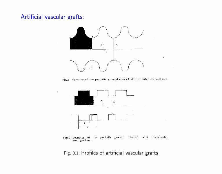
Artificial vascular grafts:
Fig. 0.1: Profiles of artificial vascular grafts

MAC method results:
Fig. 0.2: Velocity vectors - pulsatile flow
Contents
1 References 6
2 Navier-Stokes equations for incompressible viscous fluids -classical formulation 72.1 Unsteady two-dimensional flow . . . . . . . . . . . . . . . . . . . . . . . . . . . . . . 72.2 Steady two-dimensional flow . . . . . . . . . . . . . . . . . . . . . . . . . . . . . . . . 82.3 Steady 2D Stokes problem . . . . . . . . . . . . . . . . . . . . . . . . . . . . . . . . . 82.4 Unsteady axisymmetric flow . . . . . . . . . . . . . . . . . . . . . . . . . . . . . . . . 92.5 Navier-Stokes equations - variational formulation . . . . . . . . . . . . . . . . . . . . . 10
3 Approximation of the problem by FEM 113.1 Discretization of steady Navier-Stokes equations by FEM . . . . . . . . . . . . . . . . . 133.2 Discretization of unsteady Navier-Stokes equations . . . . . . . . . . . . . . . . . . . . 143.3 Space semidiscretization of unsteady Navier-Stokes equations by FEM . . . . . . . . . . 153.4 Time discretization of unsteady Navier-Stokes eqs. by the Euler method . . . . . . . . . 16
4 Splitting technique for the Navier-Stokes equations 17
5 Asymptotic behaviour of the solution near corners 18
6 A posteriori error estimates for the Stokes and NS equations 256.1 The Stokes problem and finite element solution . . . . . . . . . . . . . . . . . . . . . . 266.2 A posteriori error estimate for the Stokes problem . . . . . . . . . . . . . . . . . . . . 276.3 A posteriori estimates for 2D steady Navier-Stokes equations . . . . . . . . . . . . . . . 296.4 Example: determination of the constant C . . . . . . . . . . . . . . . . . . . . . . . . 31
6.5 Application to the adaptive mesh refinement and numerical results . . . . . . . . . . . 32
7 Application of a priori error estimates for Navier-Stokes equati-ons to very precise solution 367.1 Algorithm for generation of computational mesh . . . . . . . . . . . . . . . . . . . . . 377.2 Numerical results . . . . . . . . . . . . . . . . . . . . . . . . . . . . . . . . . . . . . . 42
8 Numerical solution of flow problems by stabilized FEM 478.1 Galerkin Least Squares stabilization technique . . . . . . . . . . . . . . . . . . . . . . 488.2 Results of numerical experiments . . . . . . . . . . . . . . . . . . . . . . . . . . . . . 508.3 Application of a posteriori error estimates . . . . . . . . . . . . . . . . . . . . . . . . . 60
9 Conclusion 63
10 References 64
1. References
[1] Girault, V., Raviart, P., G. Finite Element Method for Navier-Stokes Equations,Springer, Berlin, 1986
[2] Pironneau, O., Finite Element Methods for Fluids, J. Wiley, Chichester, 1989
[3] Turek, S., Efficient Solvers for Incompressible Flow Problems, Springer, Berlin,1991
[4] Gresho, P., M., Sani, R., L., Incompressible Flow and the Finite Element Method,J. Wiley, Chichester, 1998
[5] Glowinski, R. Finite Element Methods for Incompressible Viscous Flow, Handbookof Numerical Analysis, Vol. IX, Elsevier, 2003
[6] Donea, J., Huerta, A., Finite Element Methods for Flow Problems, J. Wiley, Chi-chester, 2003
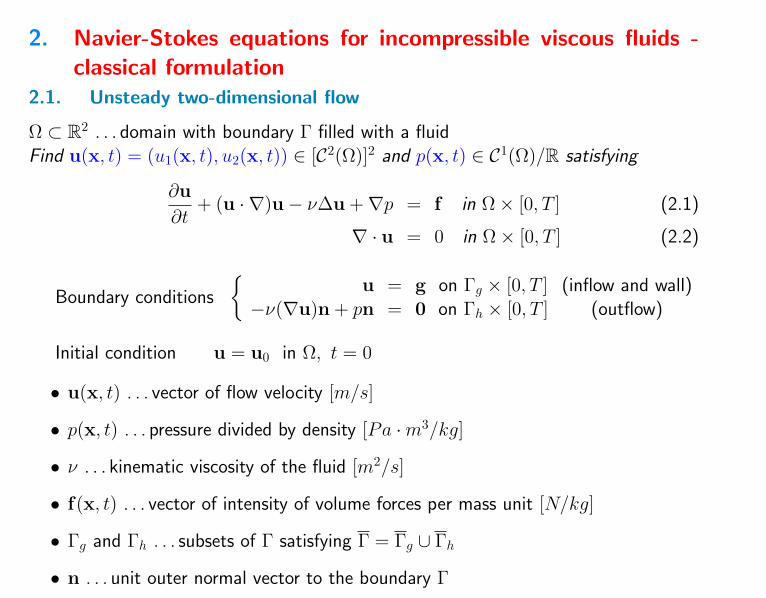
2. Navier-Stokes equations for incompressible viscous fluids -classical formulation
2.1. Unsteady two-dimensional flow
Ω ⊂ R2 . . . domain with boundary Γ filled with a fluidFind u(x, t) = (u1(x, t), u2(x, t)) ∈ [C2(Ω)]2 and p(x, t) ∈ C1(Ω)/R satisfying
∂u
∂t+ (u · ∇)u− ν∆u +∇p = f in Ω× [0, T ] (2.1)
∇ · u = 0 in Ω× [0, T ] (2.2)
Boundary conditions
u = g on Γg × [0, T ] (inflow and wall)
−ν(∇u)n + pn = 0 on Γh × [0, T ] (outflow)
Initial condition u = u0 in Ω, t = 0
• u(x, t) . . . vector of flow velocity [m/s]
• p(x, t) . . . pressure divided by density [Pa ·m3/kg]
• ν . . . kinematic viscosity of the fluid [m2/s]
• f(x, t) . . . vector of intensity of volume forces per mass unit [N/kg]
• Γg and Γh . . . subsets of Γ satisfying Γ = Γg ∪ Γh
• n . . . unit outer normal vector to the boundary Γ
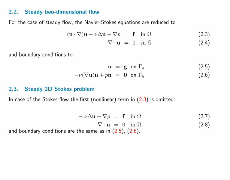
2.2. Steady two-dimensional flow
For the case of steady flow, the Navier-Stokes equations are reduced to
(u · ∇)u− ν∆u +∇p = f in Ω (2.3)
∇ · u = 0 in Ω (2.4)
and boundary conditions to
u = g on Γg (2.5)
−ν(∇u)n + pn = 0 on Γh (2.6)
2.3. Steady 2D Stokes problem
In case of the Stokes flow the first (nonlinear) term in (2.3) is omitted:
− ν∆u +∇p = f in Ω (2.7)
∇ · u = 0 in Ω (2.8)and boundary conditions are the same as in (2.5), (2.6).
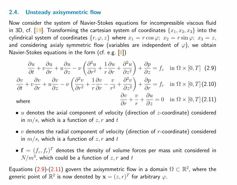
2.4. Unsteady axisymmetric flow
Now consider the system of Navier-Stokes equations for incompressible viscous fluidin 3D, cf. [19]. Transforming the cartesian system of coordinates x1, x2, x3 into thecylindrical system of coordinates r, ϕ, z where x1 = r cosϕ; x2 = r sinϕ; x3 = z,
and considering axialy symmetric flow (variables are independent of ϕ), we obtainNavier-Stokes equations in the form (cf. e.g. [8])
∂u
∂t+ v
∂u
∂r+ u
∂u
∂z− ν
(∂2u
∂r2 +1
r
∂u
∂r+∂2u
∂z2
)+∂p
∂z= fz in Ω× [0, T ] (2.9)
∂v
∂t+ v
∂v
∂r+ u
∂v
∂z− ν
(∂2v
∂r2 +1
r
∂v
∂r− v
r2 +∂2v
∂z2
)+∂p
∂r= fr in Ω× [0, T ] (2.10)
∂v
∂r+v
r+∂u
∂z= 0 in Ω× [0, T ] (2.11)where
• u denotes the axial component of velocity (direction of z-coordinate) consideredin m/s, which is a function of z, r and t
• v denotes the radial component of velocity (direction of r-coordinate) consideredin m/s, which is a function of z, r and t
• f = (fz, fr)T denotes the density of volume forces per mass unit considered in
N/m3, which could be a function of z, r and t
Equations (2.9)-(2.11) govern the axisymmetric flow in a domain Ω ⊂ R2, where thegeneric point of R2 is now denoted by x = (z, r)T for arbitrary ϕ.
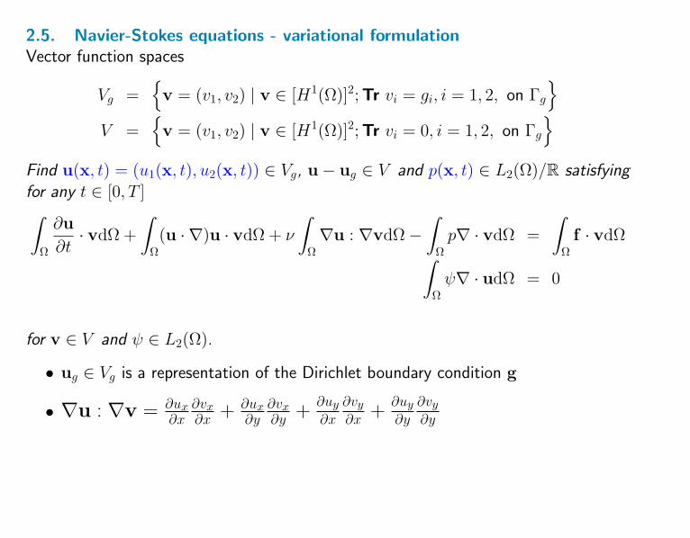
2.5. Navier-Stokes equations - variational formulationVector function spaces
Vg =v = (v1, v2) | v ∈ [H1(Ω)]2;Tr vi = gi, i = 1, 2, on Γg
V =
v = (v1, v2) | v ∈ [H1(Ω)]2;Tr vi = 0, i = 1, 2, on Γg
Find u(x, t) = (u1(x, t), u2(x, t)) ∈ Vg, u− ug ∈ V and p(x, t) ∈ L2(Ω)/R satisfyingfor any t ∈ [0, T ]∫
Ω
∂u
∂t· vdΩ +
∫Ω(u · ∇)u · vdΩ + ν
∫Ω∇u : ∇vdΩ−
∫Ωp∇ · vdΩ =
∫Ωf · vdΩ∫
Ωψ∇ · udΩ = 0
for v ∈ V and ψ ∈ L2(Ω).
• ug ∈ Vg is a representation of the Dirichlet boundary condition g
• ∇u : ∇v = ∂ux∂x
∂vx∂x + ∂ux
∂y∂vx∂y +
∂uy∂x
∂vy∂x +
∂uy∂y
∂vy∂y
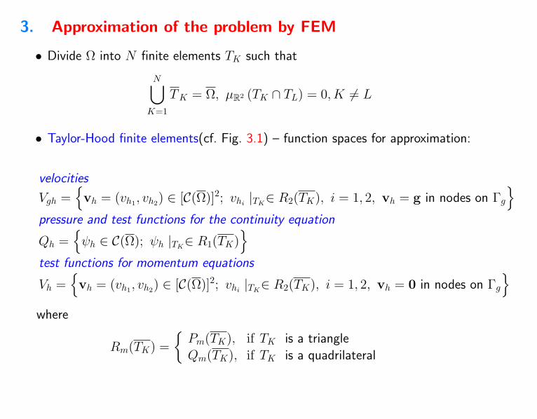
3. Approximation of the problem by FEM
• Divide Ω into N finite elements TK such that
N⋃K=1
TK = Ω, µR2 (TK ∩ TL) = 0, K 6= L
• Taylor-Hood finite elements(cf. Fig. 3.1) – function spaces for approximation:
velocities
Vgh =vh = (vh1
, vh2) ∈ [C(Ω)]2; vhi
|TK∈ R2(TK), i = 1, 2, vh = g in nodes on Γg
pressure and test functions for the continuity equation
Qh =ψh ∈ C(Ω); ψh |TK
∈ R1(TK)
test functions for momentum equations
Vh =vh = (vh1
, vh2) ∈ [C(Ω)]2; vhi
|TK∈ R2(TK), i = 1, 2, vh = 0 in nodes on Γg
where
Rm(TK) =
Pm(TK), if TK is a triangleQm(TK), if TK is a quadrilateral
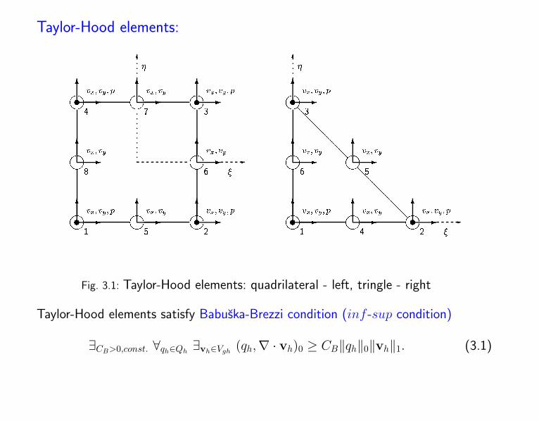
Taylor-Hood elements:
Fig. 3.1: Taylor-Hood elements: quadrilateral - left, tringle - right
Taylor-Hood elements satisfy Babuska-Brezzi condition (inf -sup condition)
∃CB>0,const. ∀qh∈Qh∃vh∈Vgh
(qh,∇ · vh)0 ≥ CB‖qh‖0‖vh‖1. (3.1)
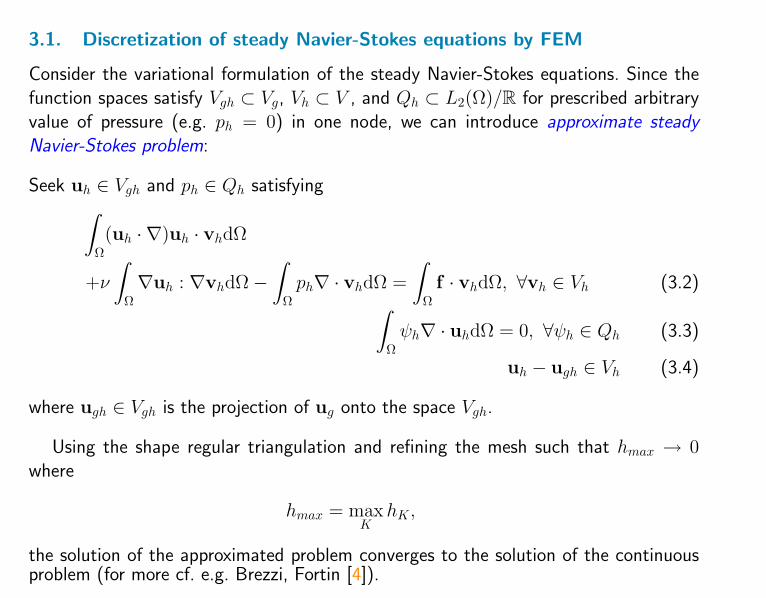
3.1. Discretization of steady Navier-Stokes equations by FEM
Consider the variational formulation of the steady Navier-Stokes equations. Since thefunction spaces satisfy Vgh ⊂ Vg, Vh ⊂ V , and Qh ⊂ L2(Ω)/R for prescribed arbitraryvalue of pressure (e.g. ph = 0) in one node, we can introduce approximate steadyNavier-Stokes problem:
Seek uh ∈ Vgh and ph ∈ Qh satisfying∫Ω(uh · ∇)uh · vhdΩ
+ν
∫Ω∇uh : ∇vhdΩ−
∫Ωph∇ · vhdΩ =
∫Ωf · vhdΩ, ∀vh ∈ Vh (3.2)∫
Ωψh∇ · uhdΩ = 0, ∀ψh ∈ Qh (3.3)
uh − ugh ∈ Vh (3.4)
where ugh ∈ Vgh is the projection of ug onto the space Vgh.
Using the shape regular triangulation and refining the mesh such that hmax → 0where
hmax = maxK
hK ,
the solution of the approximated problem converges to the solution of the continuousproblem (for more cf. e.g. Brezzi, Fortin [4]).
3.2. Discretization of unsteady Navier-Stokes equations
To solve the unsteady Navier-Stokes equations (2.1)-(2.2), we need to discretize thesystem both in space and time. Two techniques are avaiable:
• Method of lines (MOL)
1. step – semidiscretization in space (e.g. by FEM)
2. step – discretization in time (e.g. by the Euler method)
• Rothe’s method
1. step – semidiscretization in time
2. step – discretization in space
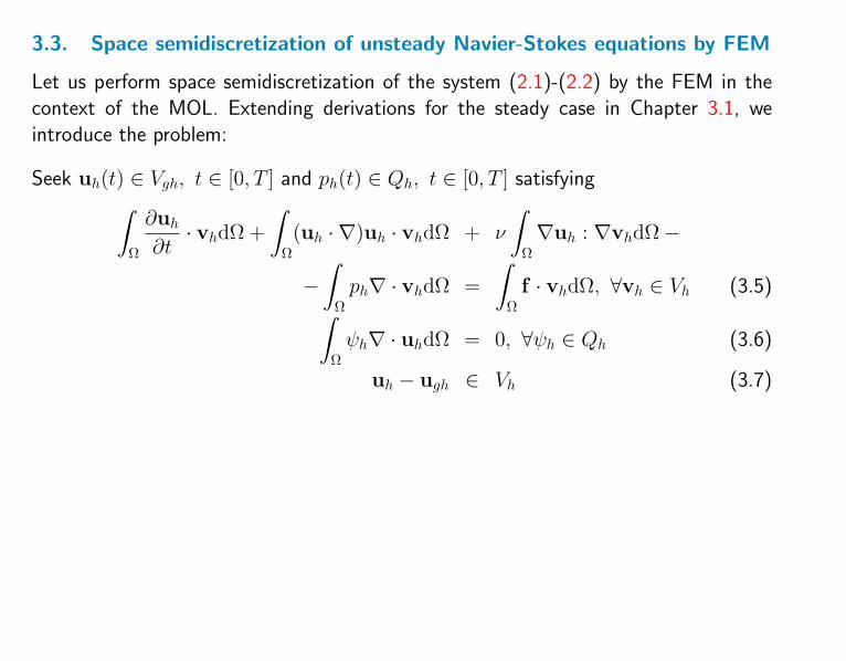
3.3. Space semidiscretization of unsteady Navier-Stokes equations by FEM
Let us perform space semidiscretization of the system (2.1)-(2.2) by the FEM in thecontext of the MOL. Extending derivations for the steady case in Chapter 3.1, weintroduce the problem:
Seek uh(t) ∈ Vgh, t ∈ [0, T ] and ph(t) ∈ Qh, t ∈ [0, T ] satisfying∫Ω
∂uh∂t
· vhdΩ +
∫Ω(uh · ∇)uh · vhdΩ + ν
∫Ω∇uh : ∇vhdΩ−
−∫
Ωph∇ · vhdΩ =
∫Ωf · vhdΩ, ∀vh ∈ Vh (3.5)∫
Ωψh∇ · uhdΩ = 0, ∀ψh ∈ Qh (3.6)
uh − ugh ∈ Vh (3.7)
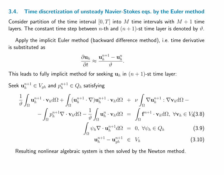
3.4. Time discretization of unsteady Navier-Stokes eqs. by the Euler method
Consider partition of the time interval [0, T ] into M time intervals with M + 1 timelayers. The constant time step between n-th and (n+ 1)-st time layer is denoted by ϑ.
Apply the implicit Euler method (backward difference method), i.e. time derivativeis substituted as
∂uh∂t
≈un+1h − unhϑ
.
This leads to fully implicit method for seeking uh in (n+ 1)-st time layer:
Seek un+1h ∈ Vgh and pn+1
h ∈ Qh satisfying
1
ϑ
∫Ωun+1h · vhdΩ +
∫Ω(un+1
h · ∇)un+1h · vhdΩ + ν
∫Ω∇un+1
h : ∇vhdΩ−
−∫
Ωpn+1h ∇ · vhdΩ− 1
ϑ
∫Ωunh · vhdΩ =
∫Ωfn+1 · vhdΩ, ∀vh ∈ Vh(3.8)∫
Ωψh∇ · un+1
h dΩ = 0, ∀ψh ∈ Qh (3.9)
un+1h − un+1
gh ∈ Vh (3.10)
Resulting nonlinear algebraic system is then solved by the Newton method.
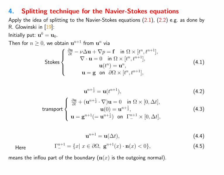
4. Splitting technique for the Navier-Stokes equationsApply the idea of splitting to the Navier-Stokes equations (2.1), (2.2) e.g. as done byR. Glowinski in [19]:
Initially put: u0 = u0.
Then for n ≥ 0, we obtain un+1 from un via
Stokes
∂u∂t − ν∆u +∇p = f in Ω× [tn, tn+1],
∇ · u = 0 in Ω× [tn, tn+1],u(tn) = un,
u = g on ∂Ω× [tn, tn+1],
(4.1)
un+ 12 = u(tn+1), (4.2)
transport
∂u∂t + (un+ 1
2 · ∇)u = 0 in Ω× [0,∆t],
u(0) = un+ 12 ,
u = gn+1(= un+ 12 ) on Γn+1
− × [0,∆t],
(4.3)
un+1 = u(∆t), (4.4)
Here Γn+1− = x| x ∈ ∂Ω, gn+1(x) · n(x) < 0, (4.5)
means the inflou part of the boundary (n(x) is the outgoing normal).
5. Asymptotic behaviour of the solution near corners
Introduction
• Motivation: numerical solution of flow of incompressible fluid in tubes with abruptchanges of diameter.
• We study the axisymmetric flow governed by the Navier-Stokes equations.
• Concern in the asymptotic behaviour of the solution near the corners.
• The asymptotic behaviour of the exact solution of the NSE in the vicinity ofthe corner is obtained using some symmetry of the principal part of the Stokesequation, and then applying the Fourier transform.
• Our aim is to make use of the information on the local behaviour of the solu-tion near the corner point, in order to suggest local meshing subordinate to theasymptotics.
• Later we present a cheap strategy to be applied to families of triangular elements.
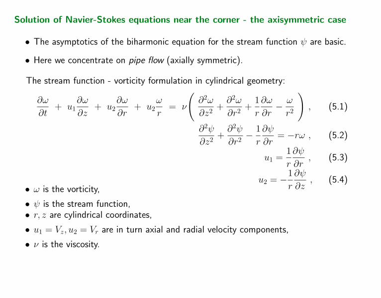
Solution of Navier-Stokes equations near the corner - the axisymmetric case
• The asymptotics of the biharmonic equation for the stream function ψ are basic.
• Here we concentrate on pipe flow (axially symmetric).
The stream function - vorticity formulation in cylindrical geometry:
∂ω
∂t+ u1
∂ω
∂z+ u2
∂ω
∂r+ u2
ω
r= ν
(∂2ω
∂z2 +∂2ω
∂r2 +1
r
∂ω
∂r− ω
r2
), (5.1)
∂2ψ
∂z2 +∂2ψ
∂r2 −1
r
∂ψ
∂r= −rω , (5.2)
u1 =1
r
∂ψ
∂r, (5.3)
u2 = −1
r
∂ψ
∂z, (5.4)
• ω is the vorticity,
• ψ is the stream function,• r, z are cylindrical coordinates,
• u1 = Vz, u2 = Vr are in turn axial and radial velocity components,
• ν is the viscosity.
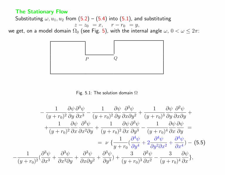
The Stationary FlowSubstituting ω, u1, u2 from (5.2) – (5.4) into (5.1), and substituting
z − z0 = x, r − r0 = y,we get, on a model domain Ω0 (see Fig. 5), with the internal angle ω, 0 < ω ≤ 2π:
P Q
Fig. 5.1: The solution domain Ω
− 1
(y + r0)2
∂ψ
∂y
∂3ψ
∂x3 −1
(y + r0)2
∂ψ
∂y
∂3ψ
∂x∂y2 +1
(y + r0)3
∂ψ
∂y
∂2ψ
∂x∂y+
+1
(y + r0)2
∂ψ
∂x
∂3ψ
∂x2∂y+
1
(y + r0)2
∂ψ
∂x
∂3ψ
∂y3 −1
(y + r0)4
∂ψ
∂x
∂ψ
∂y=
= ν 1
y + r0(∂4ψ
∂y4 + 2∂4ψ
∂y2∂x2 +∂4ψ
∂x4 )− (5.5)
− 1
(y + r0)2 (∂3ψ
∂x3 +∂3ψ
∂x2∂y+
∂3ψ
∂x∂y2 +∂3ψ
∂y3 ) +3
(y + r0)3
∂2ψ
∂x2 −3
(y + r0)4
∂ψ
∂x,
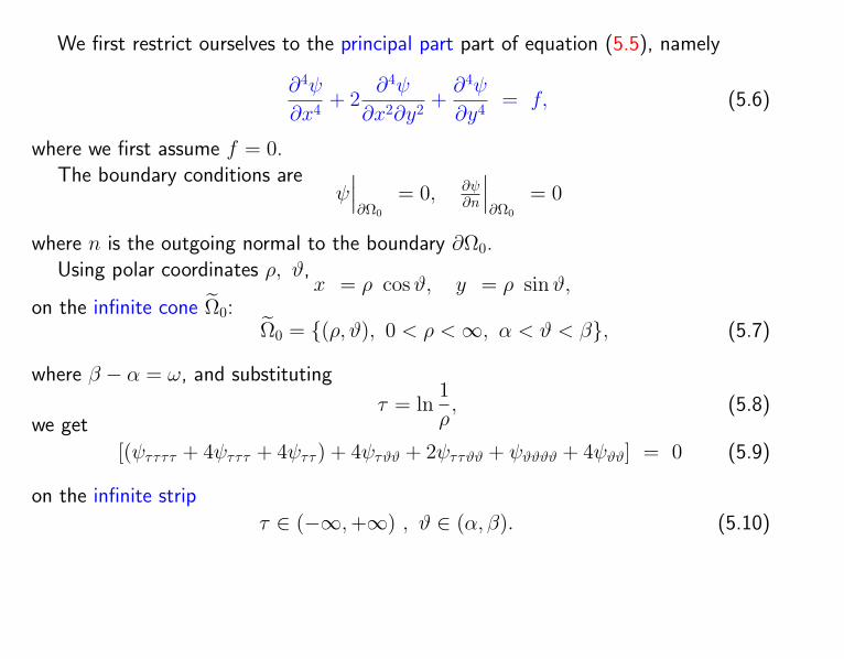
We first restrict ourselves to the principal part part of equation (5.5), namely
∂4ψ
∂x4 + 2∂4ψ
∂x2∂y2 +∂4ψ
∂y4 = f, (5.6)
where we first assume f = 0.The boundary conditions are
ψ∣∣∣∂Ω0
= 0, ∂ψ∂n
∣∣∣∂Ω0
= 0
where n is the outgoing normal to the boundary ∂Ω0.Using polar coordinates ρ, ϑ,
x = ρ cosϑ, y = ρ sinϑ,on the infinite cone Ω0:
Ω0 = (ρ, ϑ), 0 < ρ <∞, α < ϑ < β, (5.7)
where β − α = ω, and substituting
τ = ln1
ρ, (5.8)
we get
[(ψττττ + 4ψτττ + 4ψττ) + 4ψτϑϑ + 2ψττϑϑ + ψϑϑϑϑ + 4ψϑϑ] = 0 (5.9)
on the infinite strip
τ ∈ (−∞,+∞) , ϑ ∈ (α, β). (5.10)
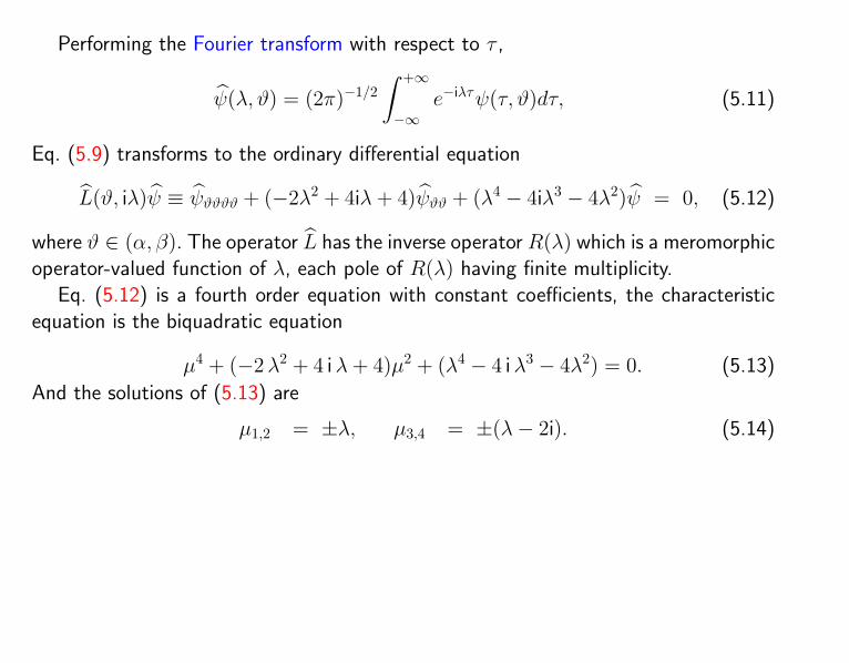
Performing the Fourier transform with respect to τ ,
ψ(λ, ϑ) = (2π)−1/2∫ +∞
−∞e−iλτψ(τ, ϑ)dτ, (5.11)
Eq. (5.9) transforms to the ordinary differential equation
L(ϑ, iλ)ψ ≡ ψϑϑϑϑ + (−2λ2 + 4iλ+ 4)ψϑϑ + (λ4 − 4iλ3 − 4λ2)ψ = 0, (5.12)
where ϑ ∈ (α, β). The operator L has the inverse operator R(λ) which is a meromorphicoperator-valued function of λ, each pole of R(λ) having finite multiplicity.
Eq. (5.12) is a fourth order equation with constant coefficients, the characteristicequation is the biquadratic equation
µ4 + (−2λ2 + 4 iλ+ 4)µ2 + (λ4 − 4 iλ3 − 4λ2) = 0. (5.13)
And the solutions of (5.13) are
µ1,2 = ±λ, µ3,4 = ±(λ− 2i). (5.14)
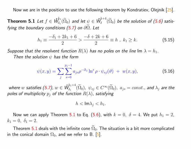
Now we are in the position to use the following theorem by Kondratiev, Olejnik [25].
Theorem 5.1 Let f ∈ Wk1
δ1(Ω0) and let ψ ∈ W
k+4δ (Ω0) be the solution of (5.6) satis-
fying the boundary conditions (5.7) on ∂Ω. Let
h1 ≡−δ1 + 2k1 + 6
2>−δ + 2k + 6
2≡ h , k1 ≥ k. (5.15)
Suppose that the resolvent function R(λ) has no poles on the line Im λ = h1.Then the solution ψ has the form
ψ(x, y) =∑j
pj−1∑s=0
ajsρ−iλj lns ρ · ψsj(ϑ) + w(x, y), (5.16)
where w satisfies (5.7), w ∈ Wk1+4δ1
(Ω0), ψsj ∈ C∞(Ω0), ajs = const., and λj are thepoles of multiplicity pj of the function R(λ), satisfying
h < Imλj < h1.
Now we can apply Theorem 5.1 to Eq. (5.6), with k = 0, δ = 4. We put h1 = 2,k1 = 0, δ1 = 2.
Theorem 5.1 deals with the infinite cone Ω0. The situation is a bit more complicatedin the conical domain Ω0, and we refer to B. [5].
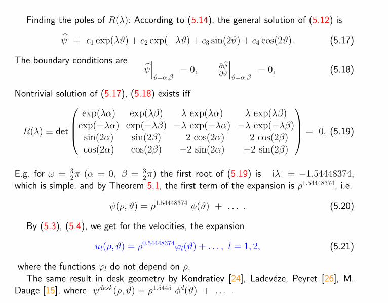
Finding the poles of R(λ): According to (5.14), the general solution of (5.12) is
ψ = c1 exp(λϑ) + c2 exp(−λϑ) + c3 sin(2ϑ) + c4 cos(2ϑ). (5.17)
The boundary conditions areψ∣∣∣ϑ=α,β
= 0, ∂ψ∂ϑ
∣∣∣ϑ=α.β
= 0, (5.18)
Nontrivial solution of (5.17), (5.18) exists iff
R(λ) ≡ det
exp(λα) exp(λβ) λ exp(λα) λ exp(λβ)
exp(−λα) exp(−λβ) −λ exp(−λα) −λ exp(−λβ)sin(2α) sin(2β) 2 cos(2α) 2 cos(2β)cos(2α) cos(2β) −2 sin(2α) −2 sin(2β)
= 0. (5.19)
E.g. for ω = 32π (α = 0, β = 3
2π) the first root of (5.19) is iλ1 = −1.54448374,which is simple, and by Theorem 5.1, the first term of the expansion is ρ1.54448374, i.e.
ψ(ρ, ϑ) = ρ1.54448374 φ(ϑ) + . . . . (5.20)
By (5.3), (5.4), we get for the velocities, the expansion
ul(ρ, ϑ) = ρ0.54448374ϕl(ϑ) + . . . , l = 1, 2, (5.21)
where the functions ϕl do not depend on ρ.The same result in desk geometry by Kondratiev [24], Ladeveze, Peyret [26], M.
Dauge [15], where ψdesk(ρ, ϑ) = ρ1.5445 φd(ϑ) + . . . .
6. A posteriori error estimates for the Stokes and NS equations
Introduction
• At present various a posteriori error estimates for the Stokes problem are available,e.g. M. Ainsworth, J.T. Oden [2], R. Verfurth [28], other references in B. [6].
• Here focus on the constant in the estimate - significant in adaptivity.
• We derive own a posteriori estimate and trace the colorblue constants and theirsources.
• In B. [6] and B. [7] a posteriori estimates for the Stokes problem in a 2D and 3D.
• Discussion of adaptive stratey
• Numerical results for a model of flow in a domain with corner singularity.
6.1. The Stokes problem and finite element solution
The Stokes problem in 2D: Ω ⊂ IR2 bounded Lipschitzian domain, given f∈ L2(Ω),find u, p ∈ H1(Ω)2 × L2
0(Ω) such that, in the weak sense,
− ν∆u +∇p = f in Ω ,
div u = 0 in Ω , (6.1)
u = 0 on ∂Ω ,
where u is the velocity vector, p is the presure, ν > 0 is the viscosity. L20(Ω) is the
space of L2 functions having mean value zero. Let us denote (., .)0 the scalar productin L2, and denote X = H1
0(Ω)2 × L20(Ω).
Stokes problem (6.1) variationally: find u, p ∈ X
ν(∇u,∇u∗)0 − (p, div u∗)0 + (p∗, div u)0 = (f ,u∗)0 ∀u∗, p∗ ∈ X. (6.2)
Finite Element Approximation
For the FEM approximation take Ω a polygon in IR2, for simplicity.Let Thh→0 be a regular (cf. [18]) family of triangulations of Ω.Vh, Qh the finite element spaces of Taylor - Hood elements, velocities and pressure areapproximated as continuous functions of spatial variables.The FEM approximation: find uh, ph ∈ Vh ×Qh such that, ∀uh
∗ , ph∗ ∈ Vh ×Qh,
ν(∇uh,∇uh∗)0 − (ph, div uh
∗)0 + (ph∗ , div uh)0 = (f ,uh∗)0 . (6.3)
6.2. A posteriori error estimate for the Stokes problem
Define the residual components on the elements K ∈ T h, by:
R1(uh, ph) = f + ν∆uh −∇ph, R2(u
h, ph) = div uh. (6.4)
The error components are defined on Ω by
eu = u− uh , ep = p− ph ,
where u, p is the exact solution defined in (6.2), uh, ph is the approximate solution,by (6.3). The X norm of eu, ep is
‖eu, ep‖2X = (eu, eu)1 + (ep, ep)0.
Using the Poincare-Friedrichs inequality, the Galerkin orthogonality, the Schwarz inequa-lity, the interpolation properties of V h, Qh, and the estimate of the solution of the dualproblem, we get the theorem (proof in B. [6] is based on the ideas of Eriksson et al.[16], and Babuska and Rheinboldt [3] )
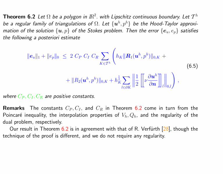
Theorem 6.2 Let Ω be a polygon in IR2. with Lipschitz continuous boundary. Let T h
be a regular family of triangulations of Ω. Let uh, ph be the Hood-Taylor approxi-mation of the solution u, p of the Stokes problem. Then the error eu, ep satisfiesthe following a posteriori estimate
‖eu‖1 + ‖ep‖0 ≤ 2 CP CI CR∑K∈T h
(hK‖R1(u
h, ph)‖0,K +
(6.5)
+ ‖R2(uh, ph)‖0,K + h
12
K
∑l∈∂K
∥∥∥∥1
2
[[ν∂uh
∂n
]]l
∥∥∥∥0,l
),
where CP , CI , CR are positive constants.
Remarks The constants CP , CI , and CR in Theorem 6.2 come in turn from thePoincare inequality, the interpolation properties of Vh, Qh, and the regularity of thedual problem, respectively.
Our result in Theorem 6.2 is in agreement with that of R. Verfurth [28], though thetechnique of the proof is different, and we do not require any regularity.

6.3. A posteriori estimates for 2D steady Navier-Stokes equations
Consider steady Navier-Stokes problem (2.1), (2.2), with boundary conditions (2.3).Discretization by finite elements again with Taylor - Hood elements P2/P1.Exact solution denoted by (u1, u2, p) and the approximate FEM solution by (uh1 , u
h2 , ph).
The difference is the error
(eu1, eu2
, ep) ≡ (u1 − uh1 , u2 − uh2 , p− ph). (6.6)
For the solution (u1, u2, p) we denote
U2(u1, u2, p,Ω) ≡ ‖(u1, u2, p)‖2V ≡ ‖(u1, u2)‖2
1,Ω + ‖p‖20,Ω (6.7)
≡∫
Ω
(u2
1 + u22 +
(∂u1
∂x
)2
+
(∂u1
∂y
)2
+
(∂u2
∂x
)2
+
(∂u2
∂y
)2)
dΩ +
∫Ωp2dΩ.
The estimate in Theorem 6.2 can be generalized to the Navier-Stokes equations:
‖(eu1, eu2
)‖21,Ω + ‖ep‖2
0,Ω ≤ E2(uh1 , uh2 , p
h), (6.8)
where (cf. [28])
E2(uh1 , uh2 , p
h,Ω) ≡ C
[∑K∈T h
h2K
∫TK
(r21 + r2
2)
+∑K∈T h
∫TK
r23dΩ
], (6.9)
where hK denotes the diameter of the element TK and ri, i = 1, 2, 3, are the residuals
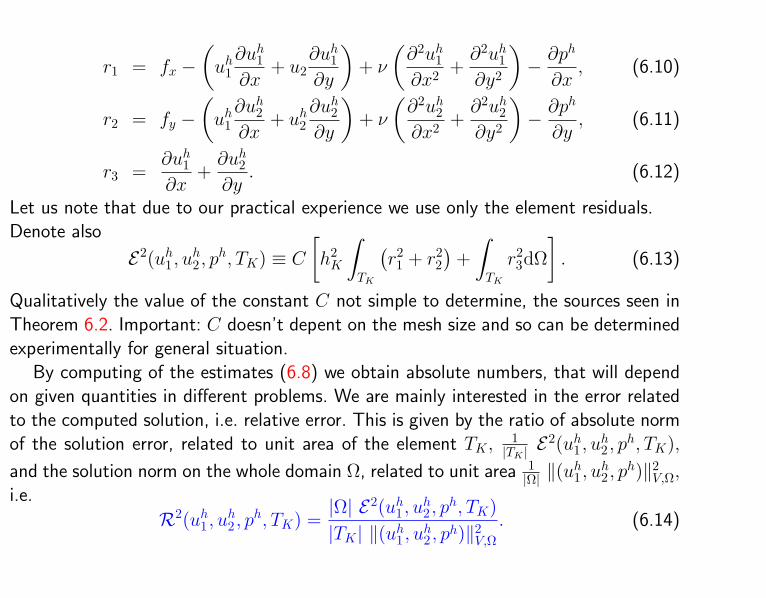
r1 = fx −(uh1∂uh1∂x
+ u2∂uh1∂y
)+ ν
(∂2uh1∂x2 +
∂2uh1∂y2
)− ∂ph
∂x, (6.10)
r2 = fy −(uh1∂uh2∂x
+ uh2∂uh2∂y
)+ ν
(∂2uh2∂x2 +
∂2uh2∂y2
)− ∂ph
∂y, (6.11)
r3 =∂uh1∂x
+∂uh2∂y
. (6.12)
Let us note that due to our practical experience we use only the element residuals.Denote also
E2(uh1 , uh2 , p
h, TK) ≡ C
[h2K
∫TK
(r21 + r2
2)
+
∫TK
r23dΩ
]. (6.13)
Qualitatively the value of the constant C not simple to determine, the sources seen inTheorem 6.2. Important: C doesn’t depent on the mesh size and so can be determinedexperimentally for general situation.
By computing of the estimates (6.8) we obtain absolute numbers, that will dependon given quantities in different problems. We are mainly interested in the error relatedto the computed solution, i.e. relative error. This is given by the ratio of absolute normof the solution error, related to unit area of the element TK ,
1|TK | E
2(uh1 , uh2 , p
h, TK),
and the solution norm on the whole domain Ω, related to unit area 1|Ω| ‖(u
h1 , u
h2 , p
h)‖2V,Ω,
i.e.
R2(uh1 , uh2 , p
h, TK) =|Ω| E2(uh1 , u
h2 , p
h, TK)
|TK | ‖(uh1 , uh2 , ph)‖2V,Ω. (6.14)
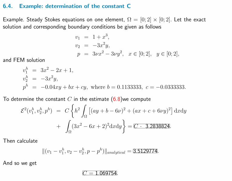
6.4. Example: determination of the constant C
Example. Steady Stokes equations on one element, Ω = [0; 2] × [0; 2]. Let the exactsolution and corresponding boundary conditions be given as follows
v1 = 1 + x3,
v2 = −3x2y,
p = 3νx2 − 3νy2, x ∈ [0; 2], y ∈ [0; 2],and FEM solution
vh1 = 3x2 − 2x+ 1,
vh2 = −3x2y,
ph = −0.04xy + bx+ cy, where b = 0.1133333, c = −0.0333333.
To determine the constant C in the estimate (6.8)we compute
E2(vh1 , vh2 , p
h) = C
h2∫
Ω
[(ay + b− 6ν)2 + (ax+ c+ 6νy)2] dxdy
+
∫Ω(3x2 − 6x+ 2)2dxdy
= C · 3.2838824.
Then calculate
‖(v1 − vh1 , v2 − vh2 , p− ph)‖analytical = 3.5129774.
And so we get
C = 1.069754.

6.5. Application to the adaptive mesh refinement and numerical results
Consider 2D flow of viscous, incompressible fluid in the domain with corner singularity(see. Fig. 6.1).
Fig. 6.1: Geometry of the channel
Due to symmetry, we solve the problem only on half of the channel, cf. Fig. 6.2. BC: onthe inflow: parabolic velocity profile, at the outflow: ’do nothing’ BC. On the upper wall:no-slip condition and on the lower wall: condition of symmetry (i.e. only y−componentof velocity equals zero). The parameters: ν = 0.0001 m2/s, vin = 1 m/s. The initialmesh is in Fig. 6.2. Relative errors on the elements of the initial mesh are on Fig. 6.3.
Fig. 6.2: Initial finite element mesh
Fig. 6.3: Relative errors on elements of initial mesh
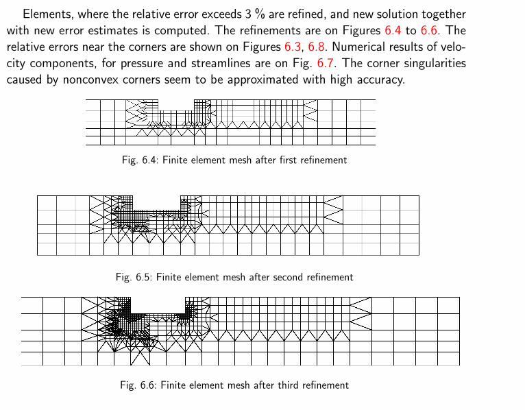
Elements, where the relative error exceeds 3 % are refined, and new solution togetherwith new error estimates is computed. The refinements are on Figures 6.4 to 6.6. Therelative errors near the corners are shown on Figures 6.3, 6.8. Numerical results of velo-city components, for pressure and streamlines are on Fig. 6.7. The corner singularitiescaused by nonconvex corners seem to be approximated with high accuracy.
Fig. 6.4: Finite element mesh after first refinement
Fig. 6.5: Finite element mesh after second refinement
Fig. 6.6: Finite element mesh after third refinement
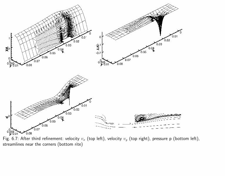
Fig. 6.7: After third refinement: velocity vx (top left), velocity vy (top right), pressure p (bottom left),streamlines near the corners (bottom rite)
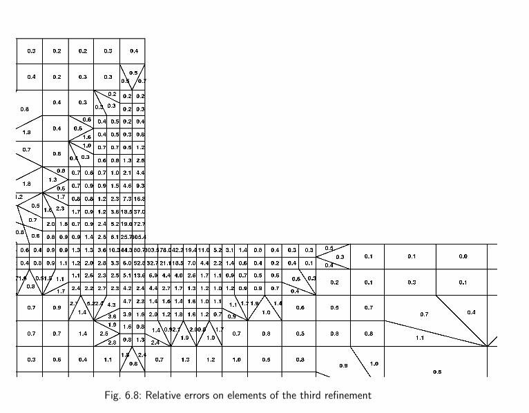
Fig. 6.8: Relative errors on elements of the third refinement
7. Application of a priori error estimates for Navier-Stokes equati-ons to very precise solution
• Incompressible viscous flow modelled by the steady Navier-Stokes equations.
• Application of theoretical results: a priori error estimates of the FEM for NSE, andasymptotic behaviour of NSE solution near corners.
• Our algorithm: generate the computational mesh in the purpose of uniform distri-bution of error on elements
• Goal: very precise FEM solution on domains with corner-like singularities.
• Usual way to improve accuracy of solution by the FEM: the adaptive mesh refine-ment based on a posteriori error estimates or error estimators. But: could be quitetime demanding, since it needs several runs of solution.
• Completely different method is applied in this chapter. Computational mesh isprepared before the first run of the solution.
• Numerical results are presented for flows in a channel with sharp obstacle and ina channel with sharp extension.
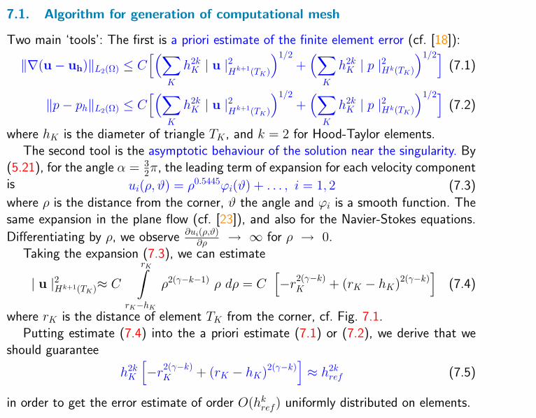
7.1. Algorithm for generation of computational mesh
Two main ‘tools’: The first is a priori estimate of the finite element error (cf. [18]):
‖∇(u− uh)‖L2(Ω) ≤ C[(∑
K
h2kK | u |2
Hk+1(TK)
)1/2+(∑
K
h2kK | p |2Hk(TK)
)1/2](7.1)
‖p− ph‖L2(Ω) ≤ C[(∑
K
h2kK | u |2
Hk+1(TK)
)1/2+(∑
K
h2kK | p |2Hk(TK)
)1/2](7.2)
where hK is the diameter of triangle TK , and k = 2 for Hood-Taylor elements.The second tool is the asymptotic behaviour of the solution near the singularity. By
(5.21), for the angle α = 32π, the leading term of expansion for each velocity component
is ui(ρ, ϑ) = ρ0.5445ϕi(ϑ) + . . . , i = 1, 2 (7.3)
where ρ is the distance from the corner, ϑ the angle and ϕi is a smooth function. Thesame expansion in the plane flow (cf. [23]), and also for the Navier-Stokes equations.
Differentiating by ρ, we observe ∂ui(ρ,ϑ)∂ρ → ∞ for ρ → 0.
Taking the expansion (7.3), we can estimate
| u |2Hk+1(TK)≈ C
rK∫rK−hK
ρ2(γ−k−1) ρ dρ = C[−r2(γ−k)
K + (rK − hK)2(γ−k)]
(7.4)
where rK is the distance of element TK from the corner, cf. Fig. 7.1.Putting estimate (7.4) into the a priori estimate (7.1) or (7.2), we derive that we
should guarantee
h2kK
[−r2(γ−k)
K + (rK − hK)2(γ−k)]≈ h2k
ref (7.5)
in order to get the error estimate of order O(hkref) uniformly distributed on elements.
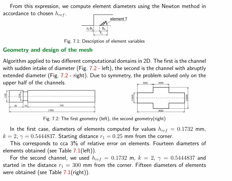
From this expression, we compute element diameters using the Newton method inaccordance to chosen href .
hT
rT
rT-h
T
element T
Fig. 7.1: Description of element variables
Geometry and design of the mesh
Algorithm applied to two different computational domains in 2D. The first is the channelwith sudden intake of diameter (Fig. 7.2 - left), the second is the channel with abruptlyextended diameter (Fig. 7.2 - right). Due to symmetry, the problem solved only on theupper half of the channels.
(185)
14530 10
Æ19
Æ25
3000 3000
9000
Æ4
00
0
Æ2
00
0
Fig. 7.2: The first geometry (left), the second geometry(right)
In the first case, diameters of elements computed for values href = 0.1732 mm,k = 2, γ = 0.5444837. Starting distance r1 = 0.25 mm from the corner.
This corresponds to cca 3% of relative error on elements. Fourteen diameters ofelements obtained (see Table 7.1(left)).
For the second channel, we used href = 0.1732 m, k = 2, γ = 0.5444837 andstarted in the distance r1 = 300 mm from the corner. Fifteen diameters of elementswere obtained (see Table 7.1(right)).
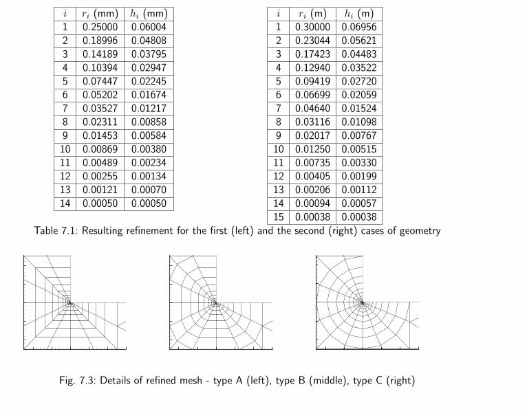
i ri (mm) hi (mm)1 0.25000 0.060042 0.18996 0.048083 0.14189 0.037954 0.10394 0.029475 0.07447 0.022456 0.05202 0.016747 0.03527 0.012178 0.02311 0.008589 0.01453 0.0058410 0.00869 0.0038011 0.00489 0.0023412 0.00255 0.0013413 0.00121 0.0007014 0.00050 0.00050
i ri (m) hi (m)1 0.30000 0.069562 0.23044 0.056213 0.17423 0.044834 0.12940 0.035225 0.09419 0.027206 0.06699 0.020597 0.04640 0.015248 0.03116 0.010989 0.02017 0.0076710 0.01250 0.0051511 0.00735 0.0033012 0.00405 0.0019913 0.00206 0.0011214 0.00094 0.0005715 0.00038 0.00038
Table 7.1: Resulting refinement for the first (left) and the second (right) cases of geometry
Fig. 7.3: Details of refined mesh - type A (left), type B (middle), type C (right)
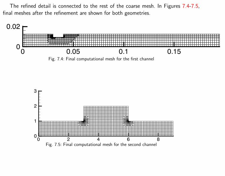
The refined detail is connected to the rest of the coarse mesh. In Figures 7.4-7.5,final meshes after the refinement are shown for both geometries.
0 0.05 0.1 0.150
0.02
Fig. 7.4: Final computational mesh for the first channel
0 2 4 6 80
1
2
3
Fig. 7.5: Final computational mesh for the second channel
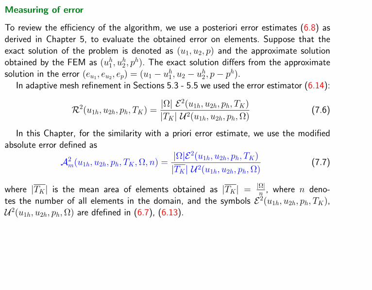
Measuring of error
To review the efficiency of the algorithm, we use a posteriori error estimates (6.8) asderived in Chapter 5, to evaluate the obtained error on elements. Suppose that theexact solution of the problem is denoted as (u1, u2, p) and the approximate solutionobtained by the FEM as (uh1 , u
h2 , p
h). The exact solution differs from the approximatesolution in the error (eu1
, eu2, ep) = (u1 − uh1 , u2 − uh2 , p− ph).
In adaptive mesh refinement in Sections 5.3 - 5.5 we used the error estimator (6.14):
R2(u1h, u2h, ph, TK) =|Ω| E2(u1h, u2h, ph, TK)
|TK | U2(u1h, u2h, ph,Ω)(7.6)
In this Chapter, for the similarity with a priori error estimate, we use the modifiedabsolute error defined as
A2m(u1h, u2h, ph, TK ,Ω, n) =
|Ω|E2(u1h, u2h, ph, TK)
|TK | U2(u1h, u2h, ph,Ω)(7.7)
where |TK | is the mean area of elements obtained as |TK | = |Ω|n , where n deno-
tes the number of all elements in the domain, and the symbols E2(u1h, u2h, ph, TK),U2(u1h, u2h, ph,Ω) are dfefined in (6.7), (6.13).
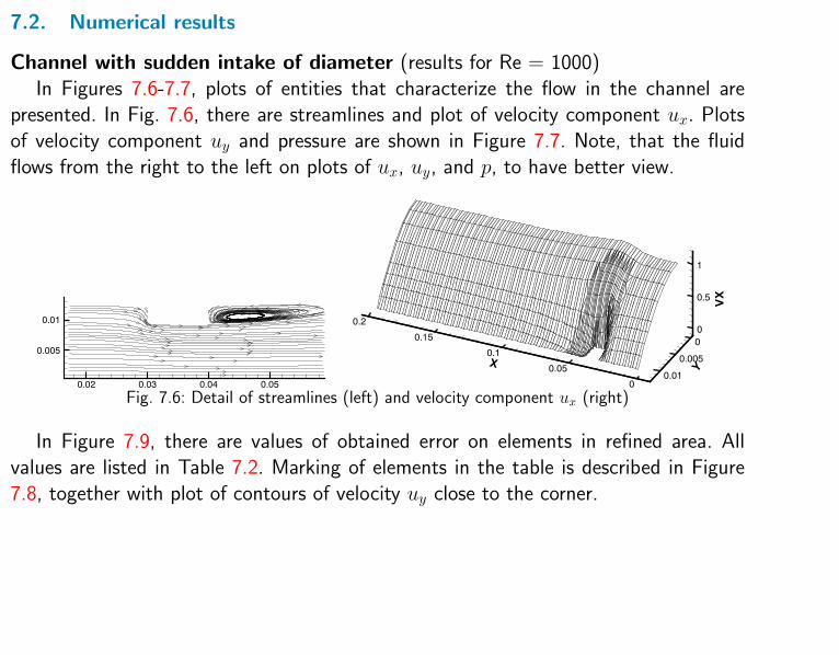
7.2. Numerical results
Channel with sudden intake of diameter (results for Re = 1000)In Figures 7.6-7.7, plots of entities that characterize the flow in the channel are
presented. In Fig. 7.6, there are streamlines and plot of velocity component ux. Plotsof velocity component uy and pressure are shown in Figure 7.7. Note, that the fluidflows from the right to the left on plots of ux, uy, and p, to have better view.
Fig. 7.6: Detail of streamlines (left) and velocity component ux (right)
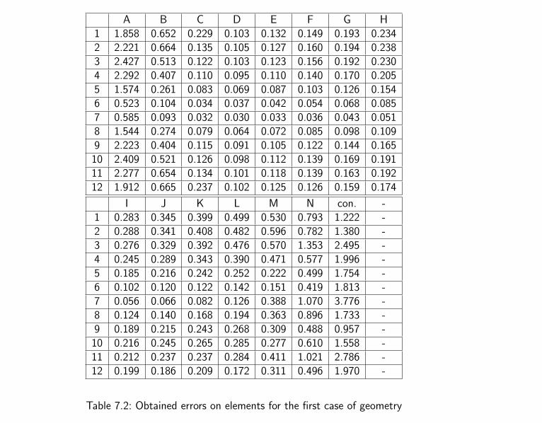
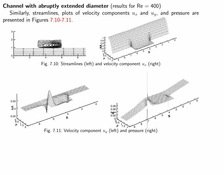
In Figure 7.9, there are values of obtained error on elements in refined area. Allvalues are listed in Table 7.2. Marking of elements in the table is described in Figure7.8, together with plot of contours of velocity uy close to the corner.
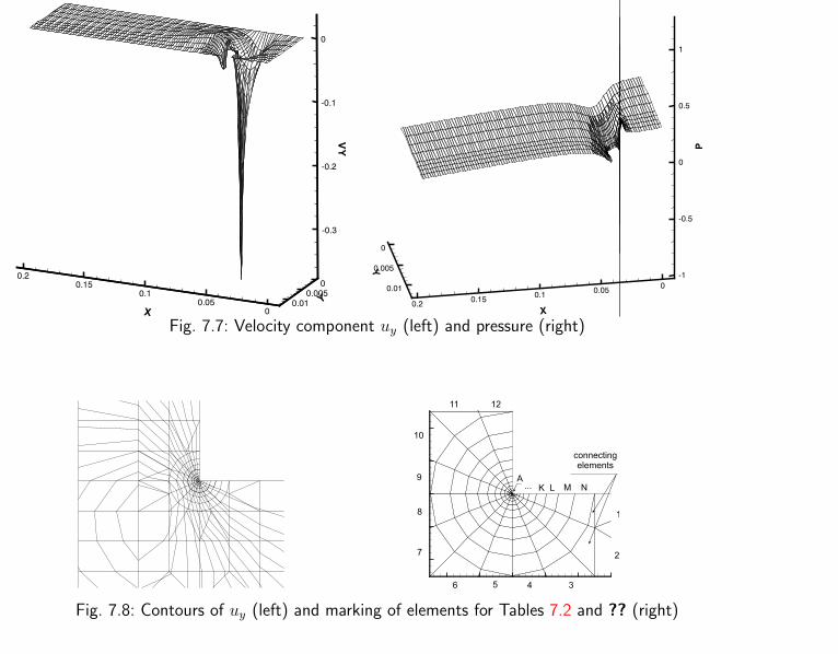
Fig. 7.7: Velocity component uy (left) and pressure (right)
Fig. 7.8: Contours of uy (left) and marking of elements for Tables 7.2 and ?? (right)
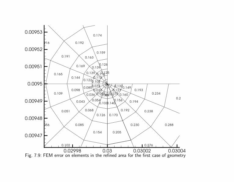
Fig. 7.9: FEM error on elements in the refined area for the first case of geometry
A B C D E F G H1 1.858 0.652 0.229 0.103 0.132 0.149 0.193 0.2342 2.221 0.664 0.135 0.105 0.127 0.160 0.194 0.2383 2.427 0.513 0.122 0.103 0.123 0.156 0.192 0.2304 2.292 0.407 0.110 0.095 0.110 0.140 0.170 0.2055 1.574 0.261 0.083 0.069 0.087 0.103 0.126 0.1546 0.523 0.104 0.034 0.037 0.042 0.054 0.068 0.0857 0.585 0.093 0.032 0.030 0.033 0.036 0.043 0.0518 1.544 0.274 0.079 0.064 0.072 0.085 0.098 0.1099 2.223 0.404 0.115 0.091 0.105 0.122 0.144 0.16510 2.409 0.521 0.126 0.098 0.112 0.139 0.169 0.19111 2.277 0.654 0.134 0.101 0.118 0.139 0.163 0.19212 1.912 0.665 0.237 0.102 0.125 0.126 0.159 0.174
I J K L M N con. -1 0.283 0.345 0.399 0.499 0.530 0.793 1.222 -2 0.288 0.341 0.408 0.482 0.596 0.782 1.380 -3 0.276 0.329 0.392 0.476 0.570 1.353 2.495 -4 0.245 0.289 0.343 0.390 0.471 0.577 1.996 -5 0.185 0.216 0.242 0.252 0.222 0.499 1.754 -6 0.102 0.120 0.122 0.142 0.151 0.419 1.813 -7 0.056 0.066 0.082 0.126 0.388 1.070 3.776 -8 0.124 0.140 0.168 0.194 0.363 0.896 1.733 -9 0.189 0.215 0.243 0.268 0.309 0.488 0.957 -10 0.216 0.245 0.265 0.285 0.277 0.610 1.558 -11 0.212 0.237 0.237 0.284 0.411 1.021 2.786 -12 0.199 0.186 0.209 0.172 0.311 0.496 1.970 -
Table 7.2: Obtained errors on elements for the first case of geometry
Channel with abruptly extended diameter (results for Re = 400)Similarly, streamlines, plots of velocity components ux and uy, and pressure are
presented in Figures 7.10-7.11.
0 2 4 6 80
1
2
3
Fig. 7.10: Streamlines (left) and velocity component ux (right)
Fig. 7.11: Velocity component uy (left) and pressure (right)

8. Numerical solution of flow problems by stabilized FEM
Motivation and goals of stabilization of FEM
• Solution of flows of incompressible viscous fluid with higher Reynolds numbers byFEM
• Stabilization techniques for FEM, Galerkin Least Squares method
• Development and implementation of an algorithm of stabilized method (semi-GLS)
• Numerical experiments
• Check of accuracy by a posteriori error estimates
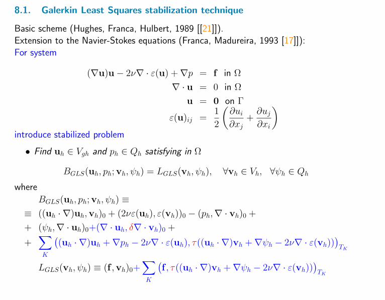
8.1. Galerkin Least Squares stabilization technique
Basic scheme (Hughes, Franca, Hulbert, 1989 [[21]]).Extension to the Navier-Stokes equations (Franca, Madureira, 1993 [17]]):For system
(∇u)u− 2ν∇ · ε(u) +∇p = f in Ω
∇ · u = 0 in Ω
u = 0 on Γ
ε(u)ij =1
2
(∂ui∂xj
+∂uj∂xi
)introduce stabilized problem
• Find uh ∈ Vgh and ph ∈ Qh satisfying in Ω
BGLS(uh, ph;vh, ψh) = LGLS(vh, ψh), ∀vh ∈ Vh, ∀ψh ∈ Qh
where
BGLS(uh, ph;vh, ψh) ≡≡ ((uh · ∇)uh,vh)0 + (2νε(uh), ε(vh))0 − (ph,∇ · vh)0 +
+ (ψh,∇ · uh)0+(∇ · uh, δ∇ · vh)0 +
+∑K
((uh · ∇)uh +∇ph − 2ν∇ · ε(uh), τ((uh · ∇)vh +∇ψh − 2ν∇ · ε(vh))
)TK
LGLS(vh, ψh) ≡ (f ,vh)0+∑K
(f , τ((uh · ∇)vh +∇ψh − 2ν∇ · ε(vh))
)TK
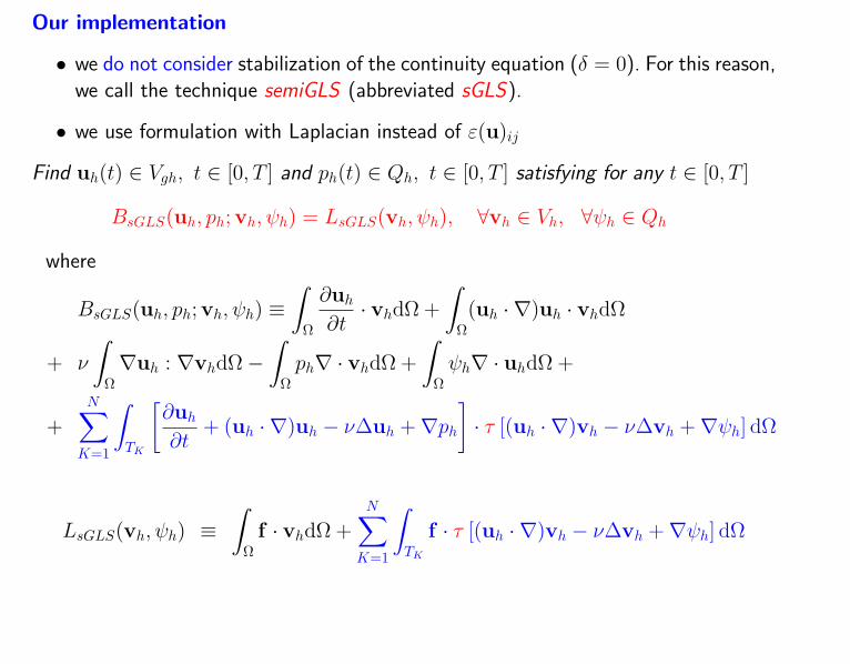
Our implementation
• we do not consider stabilization of the continuity equation (δ = 0). For this reason,we call the technique semiGLS (abbreviated sGLS).
• we use formulation with Laplacian instead of ε(u)ij
Find uh(t) ∈ Vgh, t ∈ [0, T ] and ph(t) ∈ Qh, t ∈ [0, T ] satisfying for any t ∈ [0, T ]
BsGLS(uh, ph;vh, ψh) = LsGLS(vh, ψh), ∀vh ∈ Vh, ∀ψh ∈ Qh
where
BsGLS(uh, ph;vh, ψh) ≡∫
Ω
∂uh∂t
· vhdΩ +
∫Ω(uh · ∇)uh · vhdΩ
+ ν
∫Ω∇uh : ∇vhdΩ−
∫Ωph∇ · vhdΩ +
∫Ωψh∇ · uhdΩ +
+N∑K=1
∫TK
[∂uh∂t
+ (uh · ∇)uh − ν∆uh +∇ph]· τ [(uh · ∇)vh − ν∆vh +∇ψh] dΩ
LsGLS(vh, ψh) ≡∫
Ωf · vhdΩ +
N∑K=1
∫TK
f · τ [(uh · ∇)vh − ν∆vh +∇ψh] dΩ
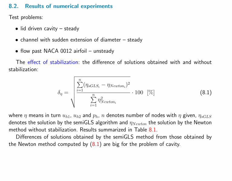
8.2. Results of numerical experiments
Test problems:
• lid driven cavity – steady
• channel with sudden extension of diameter – steady
• flow past NACA 0012 airfoil – unsteady
The effect of stabilization: the difference of solutions obtained with and withoutstabilization:
δη =
√√√√√√√n∑i=1
(ηsGLSi− ηNewtoni
)2
n∑i=1
η2Newtoni
· 100 [%] (8.1)
where η means in turn uh1, uh2 and ph, n denotes number of nodes with η given, ηsGLSdenotes the solution by the semiGLS algorithm and ηNewton the solution by the Newtonmethod without stabilization. Results summarized in Table 8.1.
Differences of solutions obtained by the semiGLS method from those obtained bythe Newton method computed by (8.1) are big for the problem of cavity.
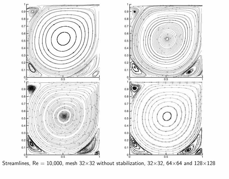
Streamlines, Re = 10,000, mesh 32×32 without stabilization, 32×32, 64×64 and 128×128
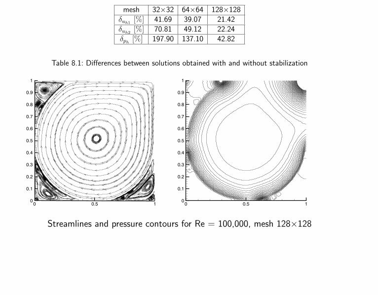
mesh 32×32 64×64 128×128δuh1
[%] 41.69 39.07 21.42δuh2
[%] 70.81 49.12 22.24δph
[%] 197.90 137.10 42.82
Table 8.1: Differences between solutions obtained with and without stabilization
Streamlines and pressure contours for Re = 100,000, mesh 128×128
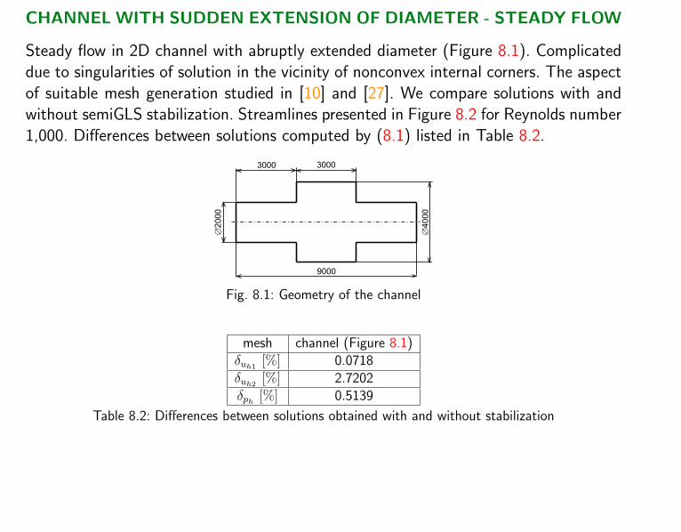
CHANNEL WITH SUDDEN EXTENSION OF DIAMETER - STEADY FLOW
Steady flow in 2D channel with abruptly extended diameter (Figure 8.1). Complicateddue to singularities of solution in the vicinity of nonconvex internal corners. The aspectof suitable mesh generation studied in [10] and [27]. We compare solutions with andwithout semiGLS stabilization. Streamlines presented in Figure 8.2 for Reynolds number1,000. Differences between solutions computed by (8.1) listed in Table 8.2.
3000 3000
9000
Æ4
00
0
Æ2
00
0
Fig. 8.1: Geometry of the channel
mesh channel (Figure 8.1)δuh1
[%] 0.0718δuh2
[%] 2.7202δph
[%] 0.5139
Table 8.2: Differences between solutions obtained with and without stabilization
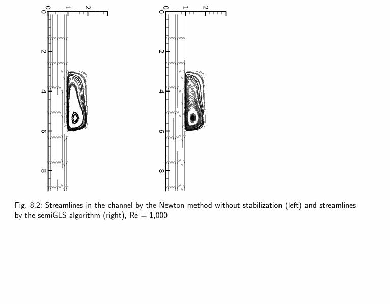
Fig. 8.2: Streamlines in the channel by the Newton method without stabilization (left) and streamlinesby the semiGLS algorithm (right), Re = 1,000
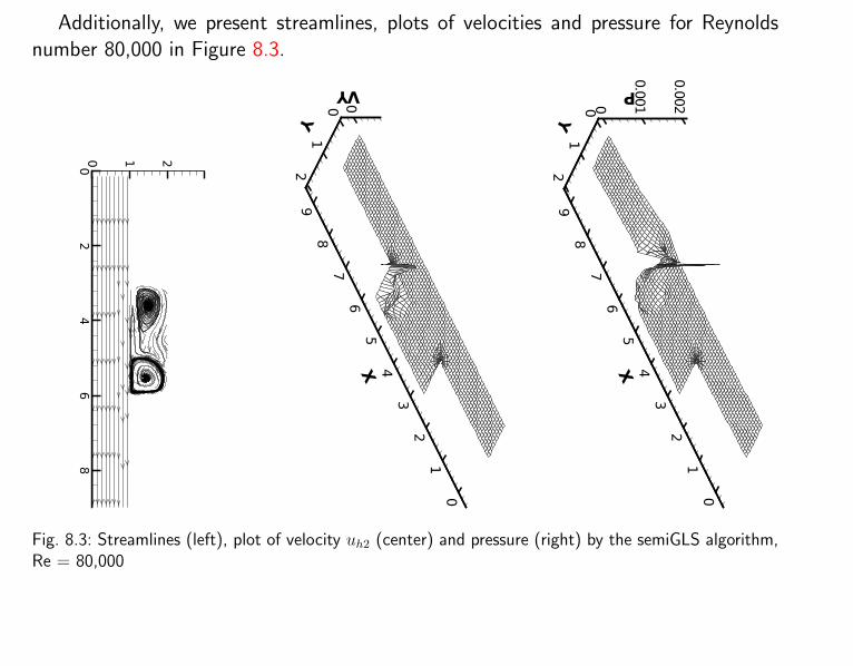
Additionally, we present streamlines, plots of velocities and pressure for Reynoldsnumber 80,000 in Figure 8.3.
Fig. 8.3: Streamlines (left), plot of velocity uh2 (center) and pressure (right) by the semiGLS algorithm,Re = 80,000
UNSTEADY SOLUTION OF FLOW PAST NACA 0012 AIRFOIL
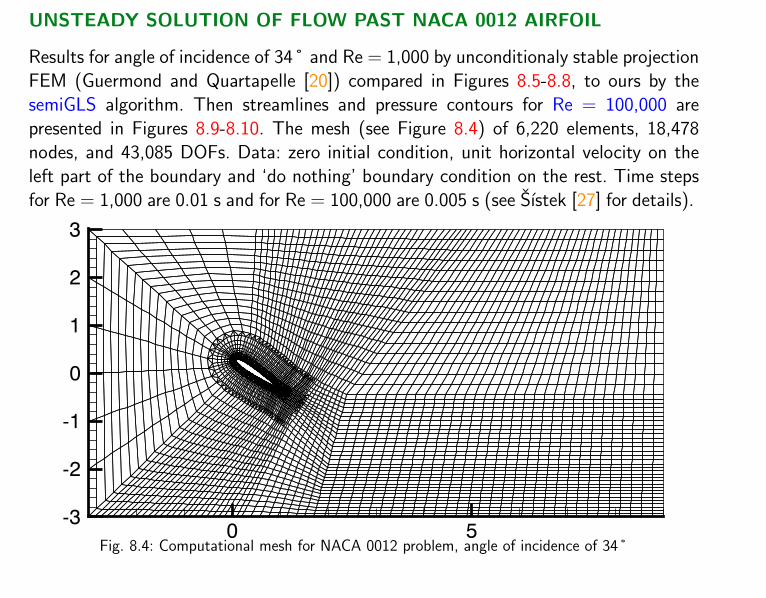
Results for angle of incidence of 34˚ and Re = 1,000 by unconditionaly stable projectionFEM (Guermond and Quartapelle [20]) compared in Figures 8.5-8.8, to ours by thesemiGLS algorithm. Then streamlines and pressure contours for Re = 100,000 arepresented in Figures 8.9-8.10. The mesh (see Figure 8.4) of 6,220 elements, 18,478nodes, and 43,085 DOFs. Data: zero initial condition, unit horizontal velocity on theleft part of the boundary and ‘do nothing’ boundary condition on the rest. Time stepsfor Re = 1,000 are 0.01 s and for Re = 100,000 are 0.005 s (see Sıstek [27] for details).
Fig. 8.4: Computational mesh for NACA 0012 problem, angle of incidence of 34˚
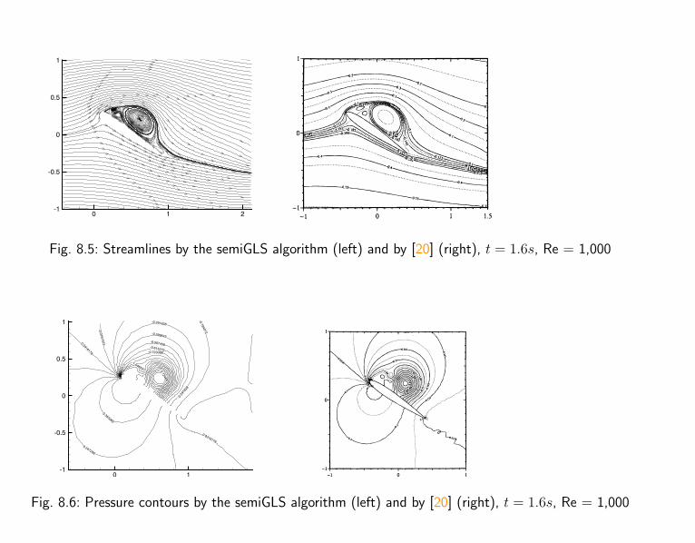
Fig. 8.5: Streamlines by the semiGLS algorithm (left) and by [20] (right), t = 1.6s, Re = 1,000
Fig. 8.6: Pressure contours by the semiGLS algorithm (left) and by [20] (right), t = 1.6s, Re = 1,000
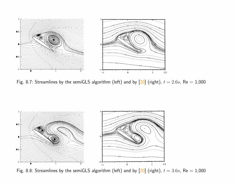
Fig. 8.7: Streamlines by the semiGLS algorithm (left) and by [20] (right), t = 2.6s, Re = 1,000
Fig. 8.8: Streamlines by the semiGLS algorithm (left) and by [20] (right), t = 3.6s, Re = 1,000
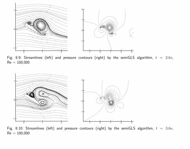
Fig. 8.9: Streamlines (left) and pressure contours (right) by the semiGLS algorithm, t = 2.6s,Re = 100,000
Fig. 8.10: Streamlines (left) and pressure contours (right) by the semiGLS algorithm, t = 3.6s,Re = 100,000
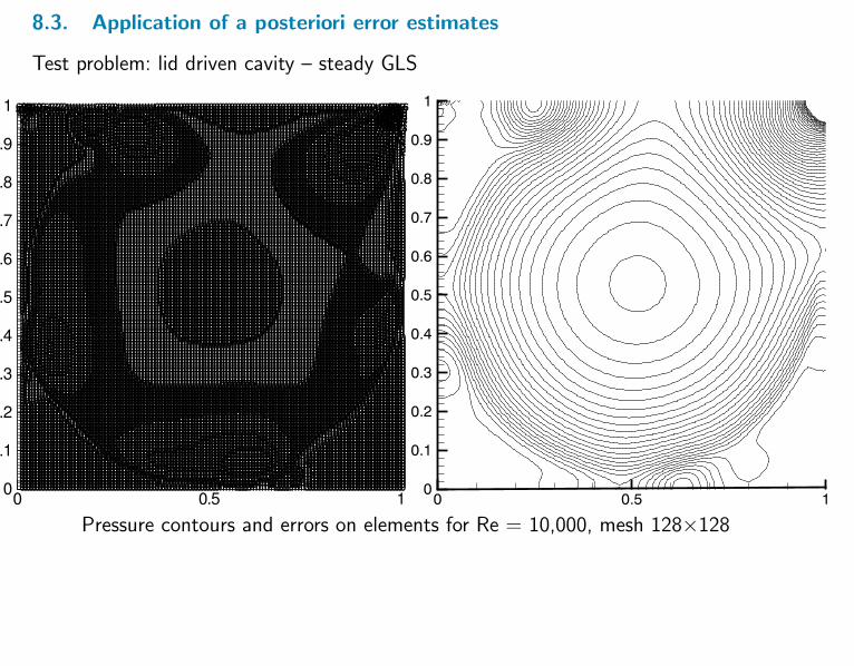
8.3. Application of a posteriori error estimates
Test problem: lid driven cavity – steady GLS
000000000000000000000000000000000000000000000000000000000000000000111111222211111111122222111110000000000000000000000000000000000000000000000000000000000000000111122233333221111122222222221111100000001111111111100000000000000000000000000000000000000000000000000000000000000000000000000000000000000000001111111111111111111222222222222221111223333322211110000000000000000000000000000000000000000000000000000000000000011122233333222222333333333333332222222222222222221111100000000000000000000000000000000000000000000000000000000000000000000000000000000000111122222333333333333333333334444444444433322222332222111100000000000000000000000000000000000000000000000000000000000001112222222223344455555555544444433333333333333333333222211100000000000000000000000000000000000000
000000000000000000000000000000000000111222333333344444444444444444444555555555555544333222222111100000000000000000000000000000000000000000000000000000000000000111111222333444555566665555554444444444444444444444433333222211100000000000000000000000000000000000000000000000000000000000000000112222333333444444444444444444444445555555666665555444332221111100000000000000000000000000000000000000000000000000000000000000000111222333444555556665555555444444444444444444444444433333332221110000000000000000000000000000000000000000000000000000000000111222233333334444444444444444444444444445555555555555544433322211110000000000000000000000000000000000000000000000000000000000000001111222233344445555555555554444444444444444444444444444333333332222111000000000000000000000000000
000000000000000000000000011122222333333333334444444444444444444444444444555555555444443333222211110000000000000000000000000000000000000000000000000000000000011112222233333444444444444444444444444444444444333333333333333333322222211100000000000000000000000000000000000000000000000111222222333333333333333333333333334444444444444444444444444433333322222211111000000000000000000000000000000000000000000000000000001111122222223333333444444444444444444444444333333333333333333333333333222222211100000000000000000000000000000000000000000011112222222233333333333333333333333333334444444444444444444444333333322222222211111100000000000000000000000000000000000000000000000111111222222222233333333344444444444444444333333333333333333333333333333222222222211110000000000000000000
000000000000000000111122222222222233333333333333333333333333333333344444444444433333333322222222222211111100000000000000000000000000000000000000000001111122222222222222233333333333333333333333333333333333333333333333333322222222222222211100000000000000000000000000000000000111222222222222222222333333333333333333333333333333333333333333333333222222222222222221111100000000000000000000000000000000000000011112222222222222222222333333333333333333333333333333333333333333333322222222222222222222211100000000000000000000000000000001111222222222222222222222222233333333333333333333333333333333333333333222222222222222222222111100000000000000000000000000000000000111222222222222222222222222233333333333333333333333333333322222222222222222222222222222222222111100000000000000
000000000000011112222222222222222222222222222222222222222222233333333333333333333222222222222222222222222222211100000000000000000000000000000001112222222222222222222222222222222222222322222222222222222222222222222222222222222222222222222222111000000000000000000000000011122222222222222222222222222222222222222222222222222222222222222222222222222222222222222222222222211000000000000000000000000000001122222222222222222222222222222222222222222222222222222222222222222222222222222222222222222222222222111000000000000101100000111222222222222222222222222222222222222222222222222222222222222222222222222222222222222222222222222222211000000000000000000000000011222222222222222222222222222222222222222222222222222222222222222222222222222222222222222222222222222222111000111110
011111111112222222222222222222222222222222222222222222222222222222222222222222222222222222222222222222222222222222210000000000000000000000011222222222222222222222222222222222222222222222222222222222222222222222222222222222222222222222222222222222111111111001111111122222333322222222222222222222222222222222222222222222222222222222222222222222222222222222222222222222222222110000000000000000000012222222222222222222222222222222222222222222222222222222222222222222222222222222222222222222222222333333332222111111100111111122333333333332222222222222222222222111111111111111111111111222222222221111111111111112222222222222222222222221100000000000000000012222222222222222222222211111111111111111111111111111111111111111111111111111112222222222222222222333333333333221111110
010111223333333333333322222222222222222111111111111111111111111111111111111111111111111111111111222222222222222222222221000000000000000012223322222222222222222211111111111111111111111111111111111111111111111111111111112222222222222223333333333333333211100000011223344444433333333222222222222221111111111111111111111111111111111111111111111111111111111112222222222222222333322210000000000000012233333222222222222222211111111111111111111111111111111111111111111111111111111111112222222222223333333344444444332110000011223444444444333333332222222222221111111111111111111111111111111111111111111111111111111111111122222222222222233333322100000000000012333333322222222222222211111111111111111111111111111111111111111111111111111111111111122222222222333333344444444443321111
111223444444444443333333222222222221111111111111111111111111111111111111111111111111111111111111112222222222222223333333321000000000012333333332222222222222211111111111111111111111111111111111111111111111111111111111111112222222222233333334444444444432212112223344455444444333333322222222222111111111111111111111111111111111111111111111111111111111111111122222222222222333333333200000000012333333333322222222222221111111111111111111111111111111111111111111111111111111111111111122222222223333334444444554444322211222344455544444443333332222222222111111111111111111111111111111111111111111111111111111111111111112222222222222333333333331000001012333443333332222222222222111111111111111111111111111111111111111111111111111111111111111112222222222333333444444455444432222
222234444544444444333333222222222211111111111111111111111111000000000011111111111111111111111111111122222222222333333344433210100111334444333333322222222222111111111111111111111111100000000000000000001111111111111111111111222222222233333344444444444433222212223344444444444433333322222222221111111111111111111000000000000000000000000011111111111111111111112222222222233333333444332110111233444333333332222222222211111111111111111111000000000000000000000000000011111111111111111122222222223333333444444444443322211222334444444444433333332222222221111111111111111110000000000000000000000000000001111111111111111111222222222223333333344443211111133444433333333222222222211111111111111111110000000000000000000000000000000011111111111111111222222222333333334444444443332221
121223344444444433333333222222222111111111111111100000000000000000000000000000000001111111111111111112222222222233333334444332211223344433333333222222222221111111111111111100000000000000000000000000000000000111111111111111122222222223333333344444443332212111122333444444333333333222222222211111111111111100000000000000000000000000000000000011111111111111111222222222223333333344433221122334443333333222222222221111111111111111100000000000000000000000000000000000001111111111111112222222222333333333334443333221111112233333333333333333322222222221111111111111100000000000000000000000000000000000000111111111111111112222222222223333333443322112233433333332222222222222111111111111111100000000000000000000000000000000000000011111111111111122222222233333333333333333222110
011122333333333333333322222222221111111111111110000000000000000000000000000000000000001111111111111111222222222222223333333332211223333333222222222222222111111111111111110000000000000000000000000000000000000001111111111111112222222222333333333333333322111000112233333333333333332222222222111111111111110000000000000000000000000000000000000000011111111111111112222222222222222333332221122233332222222222222222211111111111111110000000000000000000000000000000000000000011111111111111222222222233333333333333332211000011223333333333333333222222222211111111111111000000000000000000000000000000000000000001111111111111111122222222222222222333222112222322222222222222222211111111111111111000000000000000000000000000000000000000001111111111111122222222223333333333333332221100
001122233333333333333222222222221111111111111100000000000000000000000000000000000000000111111111111111111222222222222222222221211112222222222222222222211111111111111111100000000000000000000000000000000000000000111111111111112222222222233333333333333222110000112233333333333333322222222221111111111111110000000000000000000000000000000000000000011111111111111111122222222222222222221111111122222222222222222211111111111111111110000000000000000000000000000000000000000011111111111111122222222223333333333333332211000011223333333333333332222222222111111111111111000000000000000000000000000000000000000001111111111111111111222222222222211222111001111111111222222222211111111111111111111100000000000000000000000000000000000000001111111111111112222222222333333333333333221100
001122333333333333333222222222211111111111111100000000000000000000000000000000000000001111111111111111111112222222221111111111100011111111111222222221111111111111111111110000000000000000000000000000000000000001111111111111111222222222233333333333333322110001112233333333333333322222222221111111111111111000000000000000000000000000000000000001111111111111111111111122222211111111111000000111111111111222221111111111111111111111100000000000000000000000000000000000000111111111111111122222222223333333333333332211100111223333333333333332222222222111111111111111110000000000000000000000000000000000001111111111111111111111111222211111111111100000001111111111112221111111111111111111111111100000000000000000000000000000000000111111111111111112222222222333333333333333221110
011122333333333333333222222222211111111111111111100000000000000000000000000000000001111111111111111111111111122211111111111100000000111111111111222211111111111111111111111111000000000000000000000000000000000111111111111111111222222222233333333333333322111001012233333333333333322222222221111111111111111111000000000000000000000000000000011111111111111111111111111222221111111111100000000000111111111222222221111111111111111111111111000000000000000000000000000001111111111111111111122222222223333333333333332110100001122333333333333322222222222211111111111111111111000000000000000000000000000111111111111111111111111222222222211111111100000000000011111111122222222222111111111111111111111111000000000000000000000000011111111111111111111122222222222233333333333332211000
000012233333333333332222222222221111111111111111111111100000000000000000000001111111111111111111111122222222222222111111110000000000001111111122222222222222221111111111111111111111000000000000000000001111111111111111111111112222222222222333333333332211000000001122333333333332222222222222111111111111111111111111110000000000000000011111111111111111111112222222222222222211111111000000000000111111122222222222222222221111111111111111111111100000000000001111111111111111111111111111222222222222223333333333221000000000012223333333332222222222222221111111111111111111111111111110000000011111111111111111111111122222222222222222222111111100000000000011111122222222222222222222222111111111111111111111111111111111111111111111111111111111111222222222222222333333332221100000
000000122233333332222222222222222211111111111111111111111111111111111111111111111111111111112222222222222222222222221111110000000000011111122222222222222222222222222111111111111111111111111111111111111111111111111111111111222222222222222222333332221100000000000011222223322222222222222222222111111111111111111111111111111111111111111111111111111122222222222222222222222222211111100000000001111122222222222222222222222222221111111111111111111111111111111111111111111111111111122222222222222222222222222221100000000000000112222222222222222222222222222222111111111111111111111111111111111111111111111111122222222222222222222222222222111110000000000111122222223333333222222222222222221111111111111111111111111111111111111111111112222222222222222222222222222222221100000000
000000001122222222222222222222222222222222222211111111111111111111111111111111111111111222222222222222333333333333222221111100000000111122222333333333333332222222222222211111111111111111111111111111111111111122222222222222222222222222222222222221100000000000000000011122222222222222222222222222222222222222111111111111111111111111111111111111222222222222233333333333333333222211110000010011122223333333333333333333222222222222111111111111111111111111111111111122222222222222222222222222222222222222221100000000000000000000111222222222222222222222222222222222222222221111111111111111111111111111111222222222222233333333333333333333222111001001011122223333333333333333333332222222222221111111111111111111111111111112222222222222222222222222222222222222222211100000000000
000000000001111222222222222222222222222222222222222222221111111111111111111111111111222222222222333333333333444444333332221110101101112233334444444444333333333322222222222211111111111111111111111111222222222222222222222222222222222222222211111100000000000000000000000001111111122222222222222222332222222222222222222111111111111111111111111122222222222333333333444444444444433322211011110112233344444444444444433333333222222222221111111111111111111111112222222222222223333333333322222222222111111111100000000000000000000000000011111111112222222223333333333333322222222222221111111111111111111111112222222222233333333444444444444444333221111111111233344445555544444444333333322222222222111111111111111111111112222222222223333333333333333322222222111111110000000000000000
000000000000000001111111122222233333333333333333332222222222221111111111111111111111222222222223333333444444455555554444332211111111223344455555555544444433333332222222222211111111111111111111112222222222233333333333333333333322222111111000000000000000000000000000000000000000111112222233333344444443333333332222222222111111111111111111111122222222222333333444444555555555554443321111111123344555555555555444444333333222222222211111111111111111111112222222222333333334444444444433333222211110000000000000000000000000000000000000000001111222233334444444444444333333322222222211111111111111111111111222222222233333334444455555666655554432111221122344555666666555554444333333222222222211111111111111111111111122222222233333344444444444444433332221111100000000000000000000
00000000000000000011111122223334444455555444444333333222222221111111111111111111111111122222222233333344444555566666665554432113411234555666666665555444443333322222222111111111111111111111111111112222222333333444445555555544443332222221111000000000000000000000000000000000011122222233344445555555555444443333322222221111111111111111111111111111112222222233333444445555666666666554312563235566666666655555444433333222222221111111111111111111111111111111122222223333444445555555555544433333333221110000000000000000000000000000000011223344443344455556665555554443333322222211111111111111111111111111111111111222222233333444445555666667777653481165788877766655554444333332222222111111111111111110000001111111111111112222223333444455556666655544444455443221110000000000111101111110000000001122344555554444555666665555444433332222211111111111100000000000000011111111111111222222333333444455566788910111097131791316161412108765554443333332222221111111111111000000000000000000001111111111122222333344445555665555444455666554322110000000001111111211110000000001122345566665444445555555544443333222221111111110000000000000000000000000011111111111122222223333344456791114182223219172217273430231712975443333322222221111111111110000000000000000000000000000001111111112222233334444555444333445666654432211000000000111112521111100000000111233455666654322334444443333222221111111110000000000000000000000000000000000111111111111112222222333468121826384742211935495462382414964322111111111111111100000000000000000000000000000000000000000001111111122222333333332211234566665544332211111101011338154129148431111111111222334444443211111222222222221111111110000000000000000000000000000000000000000000000000000000000111111235913264091948821610731229732110000000000000000000000000000000000000000000000000000000000000000000000000111111111111100000001111111111222334567101220227169
0 0.5 10
0.1
0.2
0.3
0.4
0.5
0.6
0.7
0.8
0.9
1
Pressure contours and errors on elements for Re = 10,000, mesh 128×128
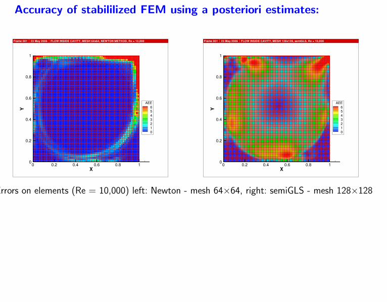
Accuracy of stabililized FEM using a posteriori estimates:
X
Y
0 0.2 0.4 0.6 0.8 10
0.2
0.4
0.6
0.8
1
AEE6543210
Frame 001 23 May 2006 FLOW INSIDE CAVITY, MESH 64x64, NEWTON METHOD, Re = 10,000
X
Y
0 0.2 0.4 0.6 0.8 10
0.2
0.4
0.6
0.8
1
AEE6543210
Frame 001 23 May 2006 FLOW INSIDE CAVITY, MESH 128x128, semiGLS, Re = 10,000
Errors on elements (Re = 10,000) left: Newton - mesh 64×64, right: semiGLS - mesh 128×128
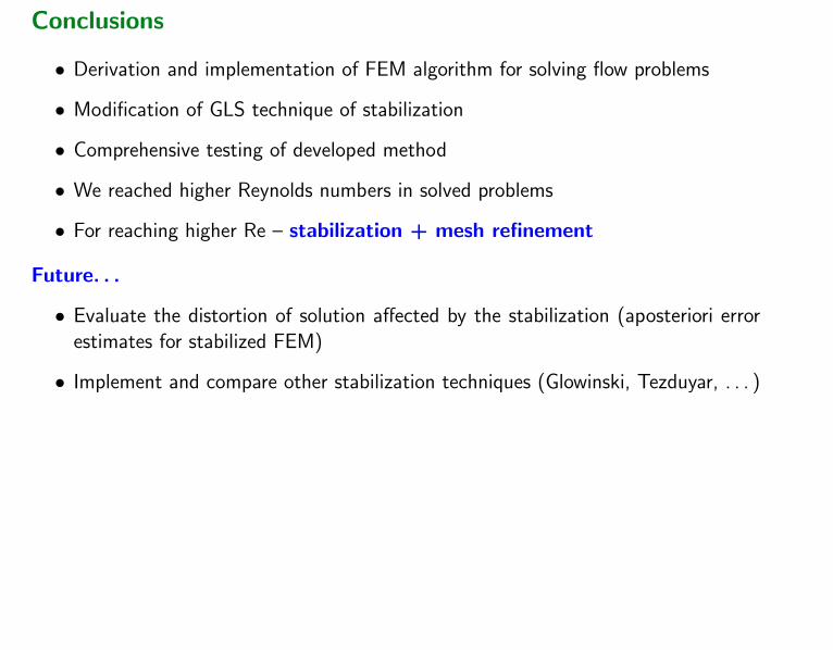
Conclusions
• Derivation and implementation of FEM algorithm for solving flow problems
• Modification of GLS technique of stabilization
• Comprehensive testing of developed method
• We reached higher Reynolds numbers in solved problems
• For reaching higher Re – stabilization + mesh refinement
Future. . .
• Evaluate the distortion of solution affected by the stabilization (aposteriori errorestimates for stabilized FEM)
• Implement and compare other stabilization techniques (Glowinski, Tezduyar, . . . )
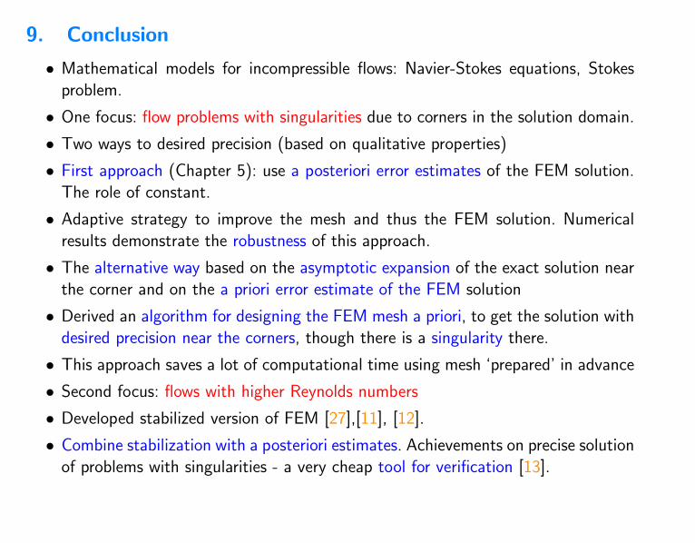
9. Conclusion
• Mathematical models for incompressible flows: Navier-Stokes equations, Stokesproblem.
• One focus: flow problems with singularities due to corners in the solution domain.
• Two ways to desired precision (based on qualitative properties)
• First approach (Chapter 5): use a posteriori error estimates of the FEM solution.The role of constant.
• Adaptive strategy to improve the mesh and thus the FEM solution. Numericalresults demonstrate the robustness of this approach.
• The alternative way based on the asymptotic expansion of the exact solution nearthe corner and on the a priori error estimate of the FEM solution
• Derived an algorithm for designing the FEM mesh a priori, to get the solution withdesired precision near the corners, though there is a singularity there.
• This approach saves a lot of computational time using mesh ‘prepared’ in advance
• Second focus: flows with higher Reynolds numbers
• Developed stabilized version of FEM [27],[11], [12].
• Combine stabilization with a posteriori estimates. Achievements on precise solutionof problems with singularities - a very cheap tool for verification [13].
10. References[1] Agmon, S., Douglis, A., Nirenberg, L., Estimates near the boundary for solutions
of elliptic partial differential equations satisfying general boundary conditions. I.,Comm. Pure Appl. Math. 12, 1959, 623-727.
[2] Ainsworth, M., Oden, J., T. (1997): A posteriori error estimators for the Stokesand Oseen problems. SIAM J. Numer. Anal., 34, 228 - 245
[3] Babuska, I., Rheinboldt, W., C. (1978): A posteriori error estimates for the finiteelement method. Internat. J. Numer. Meth. Engrg., 12, 1597 - 1615
[4] Brezzi, F., Fortin, M. Mixed and Hybrid Finite Element Methods, Springer, Berlin,1991
[5] Burda, P. On the FEM for the Navier-Stokes equations in domains with cornersingularities. In: Krızek, M., et al., editors. Finite Element Methods, Marcel Dekker,New York, 1998, 41-52
[6] Burda, P. (2000): An a posteriori error estimate for the Stokes problem in a po-lygonal domain using Hood-Taylor elements. In: Neittaanmaki, P., Tiihonen, T.,and Tarvainen, P. (eds) ENUMATH 99, Proc. of the 3-rd Europ. Conf. on Numer.Math. and Advanced Applications. World Scientific, Singapore, 448 - 455
[7] Burda, P. A posteriori error estimates for the Stokes flow in 2D and 3D domains.In: Neittaanmaki, P., Krızek, M., editors. Finite Element Methods, 3D.(GAKUTOInternat. Series, Math. Sci. and Appl., Vol. 15), Gakkotosho, Tokyo, 2001, 34-44
[8] Burda, P., Korenar, J. Numerical solution of pulsatile flow in a round tube withaxisymmetric constrictions. In: COMMUNICATIONS, Vol. 19, Institute of Hydro-dynamics, Prague, 1992, 87-110
[9] Burda, P., Novotny, J., Sousedık, B. A posteriori error estimates applied to flowin a channel with corners, Mathematics and Computers in Simulation, 61 (2003),375-383
[10] Burda, P., Novotny, J., Sıstek, J., Precise FEM solution of corner singularity usingadjusted mesh applied to axisymmetric and plane flow, ICFD Conf. Oxford, 2004,Int. J. Num. Meth. Fluids, 47, 2005, pp. 1285 - 1292.
[11] Burda, P., Novotny, J., Sıstek, J., On a modification of GLS stabilized FEM forsolving incompressible viscous flows, Int. J. Numer. Meth. Fluids, 51, 2006, 1001- 1016.
[12] Burda, P., Novotny, J., Sıstek, J., Numerical solution of flow problems by stabilizedfinite element method, Modelling 2005, Plzen, July, 2005, In: Mathematics andComputers in Simulation 76 (2007), pp. 28 - 33.
[13] Burda, P., Novotny, J., Sıstek, J., Accuracy of semiGLS stabilization of FEM forsolving Navier-Stokes equations and a posteriori error estimates, ICFD Conferenceon Numerical Methods for Fluid Dynamics, Int. J. Numer. Meth. Fluids, 56, 2008,1167 - 1173.
[14] Damasek, A., Burda, P., Finite element modelling of viscous incompressible fluidflow in glottis, ENGENEERING MECHANICS 2003, Svratka, May 12-15, 2003, In:ENGENEERING MECHANICS (CD-ROM) Praha, Ustav termomechaniky AV CR,2003, 9 pp.
[15] Dauge, Monique, Stationary Stokes system in two or three dimensional domainswith corners, Seminaire Equations aux Derivees Partielles 1987, expos
’no. 10,
Univ. de Nantes, 315-357.
[16] Eriksson, K., Estep, D., Hansbo, P., Johnson, C. (1995): Introduction to adaptivemethods for differential equations. Acta Numerica,1995, CUP, 105–158.
[17] Franca, L., P., Madureira, A., L. Element diameter free stability parameters forstabilized methods applied to fluids, Comp. Meth. Appl. Mech. Eng., 105 (1993),395-403
[18] Girault, V., Raviart, P., G. Finite Element Method for Navier-Stokes Equations,Springer, Berlin, 1986
[19] Glowinski, R. Finite Element Methods for Incompressible Viscous Flow, Handbookof Numerical Analysis, Vol. IX, Elsevier, 2003
[20] Guermond, J., L., Quartapelle, L. Calculation of viscous incompressible viscousflow by an unconditionally stable projection FEM, J. Comp. Phys., 132 (1997),12-33
[21] Hughes, T., J., R., Franca, L., P., Hulbert, G., M. A new finite element formu-lation for computational fluid dynamics: VIII. The Galerkin/least-squares methodfor advective-diffusive equations, Comp. Meth. Appl. Mech. Eng., 73 (1989), 173-189
[22] Johnson, C. Numerical Solution of Partial Differential Equations by the FiniteElement Method, Cambridge University Press, 1994
[23] Kondratiev, V., A. Asimptotika resenija uravnienija Nav’je-Stoksa v okrestnostiuglovoj tocki granicy, Prikl. Mat. i Mech., 1 (1967), 119-123
[24] Kondratiev, V. A., Krajevyje zadaci dlja ellipticeskich uravnenij v oblast’ach skonieskimi i uglovymi tockami, Trudy Moskov. Mat. obshch. 16 (1967), 209 -292.
[25] Kondratiev, V. A., Olejnik, O. A., Krajevyje zadaci dlja uravnenij s castnymi proi-zvodnzmi v negladkich oblast’ach, Uspechi Mat. Nauk 38 (1983), 3-76.
[26] Ladeveze J., Peyret, R., Calcul numerique d’une solution avec singularite desequations de Navier-Stokes: ecoulement dans un canal avec variation brusque desection, Journal de Mecanique 13 (1974), 367-396.
[27] Sıstek, J. Stabilization of finite element method for solving incompressible viscousflows, Diploma thesis, CVUT, Praha, 2004
[28] Verfurth, R. (1996): A Review of A Posteriori Error Estimation and Adaptive Mesh-Refinement Techniques. Wiley and Teubner, Chichester