finite-sample analysis of proximal gradient td …mahadeva/papers/gtduai2015.pdffinite-sample...
TRANSCRIPT
Finite-Sample Analysis of Proximal Gradient TD Algorithms
Bo LiuUMass Amherst
Ji LiuUniversity of [email protected]
Mohammad GhavamzadehAdobe & INRIA Lille
Sridhar MahadevanUMass Amherst
Marek PetrikIBM Research
Abstract
In this paper, we show for the first time how gra-dient TD (GTD) reinforcement learning methodscan be formally derived as true stochastic gradi-ent algorithms, not with respect to their originalobjective functions as previously attempted, butrather using derived primal-dual saddle-point ob-jective functions. We then conduct a saddle-pointerror analysis to obtain finite-sample bounds ontheir performance. Previous analyses of this classof algorithms use stochastic approximation tech-niques to prove asymptotic convergence, and nofinite-sample analysis had been attempted. Twonovel GTD algorithms are also proposed, namelyprojected GTD2 and GTD2-MP, which use prox-imal “mirror maps” to yield improved conver-gence guarantees and acceleration, respectively.The results of our theoretical analysis imply thatthe GTD family of algorithms are comparableand may indeed be preferred over existing leastsquares TD methods for off-policy learning, dueto their linear complexity. We provide exper-imental results showing the improved perfor-mance of our accelerated gradient TD methods.
1 INTRODUCTION
Obtaining a true stochastic gradient temporal differencemethod has been a longstanding goal of reinforcementlearning (RL) [Bertsekas and Tsitsiklis, 1996; Sutton andBarto, 1998], ever since it was discovered that the orig-inal TD method was unstable in many off-policy scenar-ios where the target behavior being learned and the ex-ploratory behavior producing samples differ. Sutton et al.[2008, 2009] proposed the family of gradient-based tem-poral difference (GTD) algorithms which offer several in-teresting properties. A key property of this class of GTDalgorithms is that they are asymptotically off-policy con-vergent, which was shown using stochastic approximation
[Borkar, 2008]. This is quite important when we noticethat many RL algorithms, especially those that are basedon stochastic approximation, such as TD(�), do not haveconvergence guarantees in the off-policy setting. Unfortu-nately, this class of GTD algorithms are not true stochasticgradient methods with respect to their original objectivefunctions, as pointed out in Szepesvari [2010]. The reasonis not surprising: the gradient of the objective functionsused involve products of terms, which cannot be sampleddirectly, and was decomposed by a rather ad-hoc splittingof terms. In this paper, we take a major step forward inresolving this problem by showing a principled way of de-signing true stochastic gradient TD algorithms by using aprimal-dual saddle point objective function, derived fromthe original objective functions, coupled with the princi-pled use of operator splitting [Bauschke and Combettes,2011].
Since in real-world applications of RL, we have access toonly a finite amount of data, finite-sample analysis of gra-dient TD algorithms is essential as it clearly shows theeffect of the number of samples (and the parameters thatplay a role in the sampling budget of the algorithm) intheir final performance. However, most of the work onfinite-sample analysis in RL has been focused on batchRL (or approximate dynamic programming) algorithms(e.g., Kakade and Langford 2002; Munos and Szepesvari2008; Antos et al. 2008; Lazaric et al. 2010a), especiallythose that are least squares TD (LSTD)-based (e.g., Lazaricet al. 2010b; Ghavamzadeh et al. 2010, 2011; Lazaric etal. 2012), and more importantly restricted to the on-policysetting. In this paper, we provide the finite-sample anal-ysis of the GTD family of algorithms, a relatively novelclass of gradient-based TD methods that are guaranteed toconverge even in the off-policy setting, and for which, tothe best of our knowledge, no finite-sample analysis hasbeen reported. This analysis is challenging because 1) thestochastic approximation methods that have been used toprove the asymptotic convergence of these algorithms donot address convergence rate analysis; 2) as we explain indetail in Section 2.1, the techniques used for the analysisof the stochastic gradient methods cannot be applied here;
3) finally, the difficulty of finite-sample analysis in the off-policy setting.
The major contributions of this paper include the first finite-sample analysis of the class of gradient TD algorithms, aswell as the design and analysis of several improved GTDmethods that result from our novel approach of formulatinggradient TD methods as true stochastic gradient algorithmsw.r.t. a saddle-point objective function. We then use thetechniques applied in the analysis of the stochastic gradi-ent methods to propose a unified finite-sample analysis forthe previously proposed as well as our novel gradient TDagorithms. Finally, given the results of our analysis, westudy the GTD class of algorithms from several differentperspectives, including acceleration in convergence, learn-ing with biased importance sampling factors, etc.
2 PRELIMINARIES
Reinforcement Learning (RL) [Bertsekas and Tsitsiklis,1996; Sutton and Barto, 1998] is a class of learning prob-lems in which an agent interacts with an unfamiliar, dy-namic and stochastic environment, where the agent’s goalis to optimize some measure of its long-term performance.This interaction is conventionally modeled as a Markovdecision process (MDP). A MDP is defined as the tuple(S,A, P a
ss
0 , R, �), where S and A are the sets of states andactions, the transition kernel P a
ss
0 specifying the probabil-ity of transition from state s 2 S to state s0 2 S by takingaction a 2 A, R(s, a) : S ⇥A ! R is the reward functionbounded by R
max
., and 0 � < 1 is a discount factor.A stationary policy ⇡ : S ⇥ A ! [0, 1] is a probabilisticmapping from states to actions. The main objective of a RLalgorithm is to find an optimal policy. In order to achievethis goal, a key step in many algorithms is to calculate thevalue function of a given policy ⇡, i.e., V ⇡
: S ! R, aprocess known as policy evaluation. It is known that V ⇡ isthe unique fixed-point of the Bellman operator T⇡ , i.e.,
V ⇡
= T⇡V ⇡
= R⇡
+ �P⇡V ⇡, (1)
where R⇡ and P⇡ are the reward function and transitionkernel of the Markov chain induced by policy ⇡. In Eq. 1,we may imagine V ⇡ as a |S|-dimensional vector and writeeverything in vector/matrix form. In the following, to sim-plify the notation, we often drop the dependence of T⇡ ,V ⇡ , R⇡ , and P⇡ to ⇡.
We denote by ⇡b
, the behavior policy that generates thedata, and by ⇡, the target policy that we would like to eval-uate. They are the same in the on-policy setting and dif-ferent in the off-policy scenario. For each state-action pair(s
i
, ai
), such that ⇡b
(ai
|si
) > 0, we define the importance-weighting factor ⇢
i
= ⇡(ai
|si
)/⇡b
(ai
|si
) with ⇢max
� 0
being its maximum value over the state-action pairs.
When S is large or infinite, we often use a linear ap-proximation architecture for V ⇡ with parameters ✓ 2
Rd and L-bounded basis functions {'i
}di=1
, i.e., 'i
:
S ! R and max
i
||'i
||1 L. We denote by �(·) =�'1
(·), . . . ,'d
(·)�> the feature vector and by F the lin-
ear function space spanned by the basis functions {'i
}di=1
,i.e., F =
�f✓
| ✓ 2 Rd and f✓
(·) = �(·)>✓
. We maywrite the approximation of V in F in the vector form asv = �✓, where � is the |S| ⇥ d feature matrix. Whenonly n training samples of the form D =
��si
, ai
, ri
=
r(si
, ai
), s0i
� n
i=1
, si
⇠ ⇠, ai
⇠ ⇡b
(·|si
), s0i
⇠P (·|s
i
, ai
), are available (⇠ is a distribution over the statespace S), we may write the empirical Bellman operator ˆTfor a function in F as
ˆT (ˆ�✓) = ˆR+ � ˆ�0✓, (2)
where ˆ
� (resp. ˆ
�
0) is the empirical feature matrix ofsize n ⇥ d, whose i-th row is the feature vector �(s
i
)
>
(resp. �(s0i
)
>), and ˆR 2 Rn is the reward vector, whose i-th element is r
i
. We denote by �i
(✓) = ri
+ ��0>i
✓� �>i
✓,the TD error for the i-th sample (s
i
, ri
, s0i
) and define��
i
= �i
� ��0i
. Finally, we define the matrices A andC, and the vector b as
A := E⇥⇢i�i(��i)
>⇤, b := E [⇢i�iri] , C := E[�i�>i ], (3)
where the expectations are w.r.t. ⇠ and P⇡b . We also denoteby ⌅, the diagonal matrix whose elements are ⇠(s), and⇠max
:= max
s
⇠(s). For each sample i in the training setD, we can calculate an unbiased estimate of A, b, and C asfollows:
ˆAi
:= ⇢i
�i
��>i
, ˆbi
:= ⇢i
ri
�i
, ˆCi
:= �i
�>i
. (4)
2.1 GRADIENT-BASED TD ALGORITHMS
The class of gradient-based TD (GTD) algorithms wereproposed by Sutton et al. [2008, 2009]. These algorithmstarget two objective functions: the norm of the expectedTD update (NEU) and the mean-square projected Bellmanerror (MSPBE), defined as (see e.g., Maei 2011)1
NEU(✓) = ||�>⌅(T v � v)||2 , (5)
MSPBE(✓) = ||v �⇧T v||2⇠ = ||�>⌅(T v � v)||2C�1
, (6)
where C = E[�i
�>i
] = �
>⌅� is the covariance matrix
defined in Eq. 3 and is assumed to be non-singular, and⇧ = �(�
>⌅�)
�1
�
>⌅ is the orthogonal projection oper-
ator into the function space F , i.e., for any bounded func-tion g, ⇧g = argmin
f2F ||g � f ||⇠
. From (5) and (6), itis clear that NEU and MSPBE are square unweighted andweighted by C�1, `
2
-norms of the quantity �
>⌅(T v� v),
respectively, and thus, the two objective functions can beunified as
J(✓) = ||�>⌅(T v� v)||2
M
�1
= ||E[⇢i
�i
(✓)�i
]||2M
�1
, (7)1It is important to note that T in (5) and (6) is T⇡ , the Bellman
operator of the target policy ⇡.

with M equals to the identity matrix I for NEU and tothe covariance matrix C for MSPBE. The second equalityin (7) holds because of the following lemma from Section4.2 in Maei [2011].Lemma 1. Let D =
��si
, ai
, ri
, s0i
� n
i=1
, si
⇠ ⇠, ai
⇠⇡b
(·|si
), s0i
⇠ P (·|si
, ai
) be a training set generated bythe behavior policy ⇡
b
and T be the Bellman operator ofthe target policy ⇡. Then, we have
�
>⌅(T v � v) = E
⇥⇢i
�i
(✓)�i
⇤= b�A✓.
Motivated by minimizing the NEU and MSPBE objectivefunctions using the stochastic gradient methods, the GTDand GTD2 algorithms were proposed with the followingupdate rules:
GTD: yt+1
= yt
+ ↵t
�⇢t
�t
(✓t
)�t
� yt
�, (8)
✓t+1
= ✓t
+ ↵t
⇢t
��t
(y>t
�t
),
GTD2: yt+1
= yt
+ ↵t
�⇢t
�t
(✓t
)� �>t
yt
��t
, (9)
✓t+1
= ✓t
+ ↵t
⇢t
��t
(y>t
�t
).
However, it has been shown that the above update rules donot update the value function parameter ✓ in the gradient di-rection of NEU and MSPBE, and thus, NEU and MSPBEare not the true objective functions of the GTD and GTD2algorithms [Szepesvari, 2010]. Consider the NEU objec-tive function in (5). Taking its gradient w.r.t. ✓, we obtain
�1
2
rNEU(✓) = ��rE
⇥⇢i
�i
(✓)�>i
⇤�E⇥⇢i
�i
(✓)�i
⇤
= ��E⇥⇢i
r�i
(✓)�>i
⇤�E⇥⇢i
�i
(✓)�i
⇤
= E⇥⇢i
��i
�>i
⇤E⇥⇢i
�i
(✓)�i
⇤. (10)
If the gradient can be written as a single expectation, thenit is straightforward to use a stochastic gradient method.However, we have a product of two expectations in (10),and unfortunately, due to the correlation between them, thesample product (with a single sample) won’t be an unbiasedestimate of the gradient. To tackle this, the GTD algorithmuses an auxiliary variable y
t
to estimate E⇥⇢i
�i
(✓)�i
⇤, and
thus, the overall algorithm is no longer a true stochasticgradient method w.r.t. NEU. It can be easily shown that thesame problem exists for GTD2 w.r.t. the MSPBE objectivefunction. This prevents us from using the standard con-vergence analysis techniques of stochastic gradient descentmethods to obtain a finite-sample performance bound forthe GTD and GTD2 algorithms.
It should be also noted that in the original publications ofGTD/GTD2 algorithms [Sutton et al., 2008, 2009], the au-thors discussed handling the off-policy scenario using bothimportance and rejected sampling. In rejected samplingthat was mainly used in Sutton et al. [2008, 2009], a sample(s
i
, ai
, ri
, s0i
) is rejected and the parameter ✓ does not up-date for this sample, if ⇡(a
i
|si
) = 0. This sampling strat-egy is not efficient since a lot of samples will be discardedif ⇡
b
and ⇡ are very different.
2.2 RELATED WORK
Before we present a finite-sample performance bound forGTD and GTD2, it would be helpful to give a briefoverview of the existing literature on finite-sample anal-ysis of the TD algorithms. The convergence rate of theTD algorithms mainly depends on (d, n, ⌫), where d isthe size of the approximation space (the dimension of thefeature vector), n is the number of samples, and ⌫ is thesmallest eigenvalue of the sample-based covariance matrixˆC =
ˆ
�
>ˆ
�, i.e., ⌫ = �min
(
ˆC).
Antos et al. [2008] proved an error bound of O(
d log d
n
1/4 ) forLSTD in bounded spaces. Lazaric et al. [2010b] proposeda LSTD analysis in leaner spaces and obtained a tighter
bound of O(
qd log d
n⌫
) and later used it to derive a bound forthe least-squares policy iteration (LSPI) algorithm [Lazaricet al., 2012]. Tagorti and Scherrer [2014] recently proposedthe first convergence analysis for LSTD(�) and derived abound of ˜O(d/⌫
pn). The analysis is a bit different than
the one in Lazaric et al. [2010b] and the bound is weaker interms of d and ⌫. Another recent result is by Prashanthet al. [2014] that use stochastic approximation to solveLSTD(0), where the resulting algorithm is exactly TD(0)
with random sampling (samples are drawn i.i.d. and notfrom a trajectory), and report a Markov design bound (thebound is computed only at the states used by the algorithm)of O(
qd
n⌫
) for LSTD(0). All these results are for the on-policy setting, except the one by Antos et al. [2008] thatalso holds for the off-policy formulation. Another workin the off-policy setting is by Avila Pires and Szepesvari[2012] that uses a bounding trick and improves the resultof Antos et al. [2008] by a log d factor.
The line of research reported here has much in commonwith work on proximal reinforcement learning [Mahade-van et al., 2014], which explores first-order reinforcementlearning algorithms using mirror maps [Bubeck, 2014; Ju-ditsky et al., 2008] to construct primal-dual spaces. Thiswork began originally with a dual space formulation offirst-order sparse TD learning [Mahadevan and Liu, 2012].A saddle point formulation for off-policy TD learning wasinitially explored in Liu et al. [2012], where the objectivefunction is the norm of the approximation residual of a lin-ear inverse problem [Avila Pires and Szepesvari, 2012]. Asparse off-policy GTD2 algorithm with regularized dual av-eraging is introduced by Qin and Li [2014]. These studiesprovide different approaches to formulating the problem,first as a variational inequality problem [Juditsky et al.,2008; Mahadevan et al., 2014] or as a linear inverse prob-lem [Liu et al., 2012], or as a quadratic objective function(MSPBE) using two-time-scale solvers [Qin and Li, 2014].In this paper, we are going to explore the true nature ofthe GTD algorithms as stochastic gradient algorithm w.r.tthe convex-concave saddle-point formulations of NEU andMSPBE.
3 SADDLE-POINT FORMULATION OFGTD ALGORITHMS
In this section, we show how the GTD and GTD2 algo-rithms can be formulated as true stochastic gradient (SG)algorithms by writing their respective objective functions,NEU and MSPBE, in the form of a convex-concave saddle-point. As discussed earlier, this new formulation of GTDand GTD2 as true SG methods allows us to use the con-vergence analysis techniques for SGs in order to derivefinite-sample performance bounds for these RL algorithms.Moreover, it allows us to use more efficient algorithms thathave been recently developed to solve SG problems, suchas stochastic Mirror-Prox (SMP) [Juditsky et al., 2008], toderive more efficient versions of GTD and GTD2.
A particular type of convex-concave saddle-point formula-tion is formally defined as
min
✓
max
y
�L(✓, y) = hb�A✓, yi+ F (✓)�K(y)
�, (11)
where F (✓) is a convex function and K(y) is a smoothconvex function such that
K(y)�K(x)� hrK(x), y � xi LK
2
||x� y||2. (12)
Next we follow Juditsky et al. [2008]; Nemirovski et al.[2009]; Chen et al. [2013] and define the following errorfunction for the saddle-point problem (11).Definition 1. The error function of the saddle-point prob-lem (11) at each point (✓0, y0) is defined as
Err(✓0, y0) = max
y
L(✓0, y)�min
✓
L(✓, y0). (13)
In this paper, we consider the saddle-point problem (11)with F (✓) = 0 and K(y) = 1
2
||y||2M
, i.e.,
min
✓
max
y
⇣L(✓, y) = hb�A✓, yi � 1
2
||y||2M
⌘, (14)
where A and b were defined by Eq. 3, and M is a positivedefinite matrix. It is easy to show that K(y) =
1
2
||y||2M
satisfies the condition in Eq. 12.
We first show in Proposition 1 that if (✓⇤, y⇤) is the saddle-point of problem (14), then ✓⇤ will be the optimum of NEUand MSPBE defined in Eq. 7. We then prove in Proposi-tion 2 that GTD and GTD2 in fact find this saddle-point.Proposition 1. For any fixed ✓, we have 1
2
J(✓) =
max
y
L(✓, y), where J(✓) is defined by Eq. 7.
Proof. Since L(✓, y) is an unconstrained quadratic pro-gram w.r.t. y, the optimal y⇤(✓) = argmax
y
L(✓, y) canbe analytically computed as
y⇤(✓) = M�1
(b�A✓). (15)
The result follows by plugging y⇤ into (14) and using thedefinition of J(✓) in Eq. 7 and Lemma 1.
Proposition 2. GTD and GTD2 are true stochastic gradi-ent algorithms w.r.t. the objective function L(✓, y) of thesaddle-point problem (14) with M = I and M = C =
�
>⌅� (the covariance matrix), respectively.
Proof. It is easy to see that the gradient updates of thesaddle-point problem (14) (ascending in y and descendingin ✓) may be written as
yt+1
= yt
+ ↵t
(b�A✓t
�Myt
) , (16)✓t+1
= ✓t
+ ↵t
A>yt
.
We denote ˆM := 1 (resp. ˆM :=
ˆC) for GTD (resp.GTD2). We may obtain the update rules of GTD andGTD2 by replacing A, b, and C in (16) with their unbi-ased estimates ˆA, ˆb, and ˆC from Eq. 4, which completesthe proof.
4 FINITE-SAMPLE ANALYSIS
In this section, we provide a finite-sample analysis for arevised version of the GTD/GTD2 algorithms. We first de-scribe the revised GTD algorithms in Section 4.1 and thendedicate the rest of Section 4 to their sample analysis. Notethat from now on we use the M matrix (and its unbiasedestimate ˆM
t
) to have a unified analysis for GTD and GTD2algorithms. As described earlier, M is replaced by the iden-tity matrix I in GTD and by the covariance matrix C (andits unbiased estimate ˆC
t
) in GTD2.
4.1 THE REVISED GTD ALGORITHMS
The revised GTD algorithms that we analyze in this pa-per (see Algorithm 1) have three differences with the stan-dard GTD algorithms of Eqs. 8 and 9 (and Eq. 16). 1) Weguarantee that the parameters ✓ and y remain bounded byprojecting them onto bounded convex feasible sets ⇥ andY defined in Assumption 2. In Algorithm 1, we denoteby ⇧
⇥
and ⇧
Y
, the projection into sets ⇥ and Y , respec-tively. This is standard in stochastic approximation algo-rithms and has been used in off-policy TD(�) [Yu, 2012]and actor-critic algorithms (e.g., Bhatnagar et al. 2009). 2)after n iterations (n is the number of training samples in D),the algorithms return the weighted (by the step size) aver-age of the parameters at all the n iterations (see Eq. 18).3) The step-size ↵
t
is selected as described in the proofof Proposition 3 in the supplementary material. Note thatthis fixed step size of O(1/
pn) is required for the high-
probability bound in Proposition 3 (see Nemirovski et al.2009 for more details).
4.2 ASSUMPTIONS
In this section, we make several assumptions on the MDPand basis functions that are used in our finite-sample anal-ysis of the revised GTD algorithms. These assumptions are

Algorithm 1 Revised GTD Algorithms1: for t = 1, . . . , n do2: Update parameters
yt+1
= ⇧Y
⇣yt + ↵t(
ˆbt � ˆAt✓t � ˆMtyt)⌘
✓t+1
= ⇧
⇥
⇣✓t + ↵t
ˆA>t yt
⌘(17)
3: end for4: OUTPUT
¯✓n :=
Pnt=1
↵t✓tPnt=1
↵t, yn :=
Pnt=1
↵tytPnt=1
↵t(18)
quite standard and are similar to those made in the priorwork on GTD algorithms [Sutton et al., 2008, 2009; Maei,2011] and those made in the analysis of SG algorithms [Ne-mirovski et al., 2009].Assumption 2. (Feasibility Sets) We define the boundedclosed convex sets ⇥ ⇢ Rd and Y ⇢ Rd as the feasible setsin Algorithm 1. We further assume that the saddle-point(✓⇤, y⇤) of the optimization problem (14) belongs to ⇥⇥Y .We also define D
✓
:=
⇥max
✓2⇥
||✓||22
�min
✓2⇥
||✓||22
⇤1/2,
Dy
:=
⇥max
y2Y
||y||22
� min
y2Y
||y||22
⇤1/2, and R =
max
�max
✓2⇥
||✓||2
,max
y2Y
||y||2
.
Assumption 3. (Non-singularity) We assume that thecovariance matrix C = E[�
i
�>i
] and matrix A =
E⇥⇢i
�i
(��i
)
>⇤ are non-singular.Assumption 4. (Boundedness) Assume the features(�
i
,�0
i
) have uniformly bounded second moments. Thistogether with the boundedness of features (by L) and im-portance weights (by ⇢
max
) guarantees that the matrices Aand C, and vector b are uniformly bounded.
This assumption guarantees that for any (✓, y) 2 ⇥ ⇥ Y ,the unbiased estimators of b�A✓ �My and A>y, i.e.,
E[ˆbt
� ˆAt
✓ � ˆMt
y] = b�A✓ �My,
E[ ˆA>t
y] = A>y, (19)
all have bounded variance, i.e.,
E⇥||ˆb
t
� ˆAt
✓ � ˆMt
y � (b�A✓ �My)||2⇤ �2
1
,
E⇥|| ˆA>
t
y �A>y||2⇤ �2
2
, (20)
where �1
and �2
are non-negative constants. We furtherdefine
�2
= �2
1
+ �2
2
. (21)
Assumption 4 also gives us the following “light-tail” as-sumption. There exist constants M⇤,✓ and M⇤,y such that
E[exp{ ||ˆbt � ˆAt✓ � ˆMty||2
M2
⇤,✓
}] exp{1},
E[exp{ ||ˆA>t y||2
M2
⇤,y}] exp{1}. (22)
This “light-tail” assumption is equivalent to the assumptionin Eq. 3.16 in Nemirovski et al. [2009] and is necessary forthe high-probability bound of Proposition 3. We will showhow to compute M⇤,✓,M⇤,y in the Appendix.
4.3 FINITE-SAMPLE PERFORMANCE BOUNDS
The finite-sample performance bounds that we derive forthe GTD algorithms in this section are for the case that thetraining set D has been generated as discussed in Section 2.We further discriminate between the on-policy (⇡ = ⇡
b
)and off-policy (⇡ 6= ⇡
b
) scenarios. The sampling schemeused to generate D, in which the first state of each tuple,si
, is an i.i.d. sample from a distribution ⇠, also consideredin the original GTD and and GTD2 papers, for the anal-ysis of these algorithms, and not in the experiments [Sut-ton et al., 2008, 2009]. Another scenario that can motivatethis sampling scheme is when we are given a set of high-dimensional data generated either in an on-policy or off-policy manner, and d is so large that the value function ofthe target policy cannot be computed using a least-squaresmethod (that involves matrix inversion), and iterative tech-niques similar to GTD/GTD2 are required.
We first derive a high-probability bound on the error func-tion of the saddle-point problem (14) at the GTD solution(
¯✓n
, yn
). Before stating this result in Proposition 3, we re-port the following lemma that is used in its proof.Lemma 2. The induced `
2
-norm of matrix A and the `2
-norm of vector b are bounded by
||A||2
(1 + �)⇢max
L2d, ||b||2
⇢max
LRmax
. (23)
Proof. See the supplementary material.
Proposition 3. Let (¯✓n
, yn
) be the output of the GTD algo-rithm after n iterations (see Eq. 18). Then, with probabilityat least 1� �, we have
Err(
¯✓n
, yn
) r
5
n(8 + 2 log
2
�)R2 (24)
⇥✓⇢max
L⇣2(1 + �)Ld+
Rmax
R
⌘+ ⌧ +
�
R
◆,
where Err(
¯✓n
, yn
) is the error function of the saddle-pointproblem (14) defined by Eq. 13, R defined in Assump-tion 2, � is from Eq. 21, and ⌧ = �
max
(M) is the largestsingular value of M , which means ⌧ = 1 for GTD and⌧ = �
max
(C) for GTD2.
Proof. See the supplementary material.
Theorem 1. Let ¯✓n
be the output of the GTD algorithmafter n iterations (see Eq. 18). Then, with probability atleast 1� �, we have
1
2
||A¯✓n
� b||2⇠
⌧⇠max
Err(
¯✓n
, yn
). (25)

Proof. From Proposition 1, for any ✓, we have
max
y
L(✓, y) =1
2
||A✓ � b||2M
�1
.
Given Assumption 3, the system of linear equations A✓ = bhas a solution ✓⇤, i.e., the (off-policy) fixed-point ✓⇤ exists,and thus, we may write
min
✓
max
y
L(✓, y) = min
✓
1
2
||A✓ � b||2M
�1
=
1
2
||A✓⇤ � b||2M
�1
= 0.
In this case, we also have2
min
✓
L(✓, y) max
y
min
✓
L(✓, y) min
✓
max
y
L(✓, y)
=
1
2
||A✓⇤ � b||2M
�1
= 0. (26)
From Eq. 26, for any (✓, y) 2 ⇥ ⇥ Y including (
¯✓n
, yn
),we may write
Err(
¯✓n
, yn
) = max
y
L(¯✓n
, y)�min
✓
L(✓, yn
) (27)
� max
y
L(¯✓n
, y) =1
2
||A¯✓n
� b||2M
�1
.
Since ||A¯✓n
�b||2⇠
⌧⇠max
||A¯✓n
�b||2M
�1
, where ⌧ is thelargest singular value of M , we have
1
2
||A¯✓n
�b||2⇠
⌧⇠max
2
||A¯✓n
�b||2M
�1
⌧⇠max
Err(
¯✓n
, yn
).
(28)The proof follows by combining Eqs. 28 and Proposition 3.It completes the proof.
With the results of Proposition 3 and Theorem 1, we arenow ready to derive finite-sample bounds on the perfor-mance of GTD/GTD2 in both on-policy and off-policy set-tings.
4.3.1 On-Policy Performance Bound
In this section, we consider the on-policy setting in whichthe behavior and target policies are equal, i.e., ⇡
b
= ⇡, andthe sampling distribution ⇠ is the stationary distribution ofthe target policy ⇡ (and the behavior policy ⇡
b
). We useLemma 3 to derive our on-policy bound. The proof of thislemma can be found in Geist et al. [2012].Lemma 3. For any parameter vector ✓ and correspondingv = �✓, the following equality holds
V � v = (I � �⇧P )
�1
⇥(V �⇧V ) + �C�1
(b�A✓)⇤. (29)
Using Lemma 3, we derive the following performancebound for GTD/GTD2 in the on-policy setting.
2We may write the second inequality as an equality for oursaddle-point problem defined by Eq. 14.
Proposition 4. Let V be the value of the target policy andvn
= �
¯✓n
, where ¯✓n
defined by (18), be the value functionreturned by on-policy GTD/GTD2. Then, with probabilityat least 1� �, we have
||V�vn||⇠ 1
1� �
✓||V �⇧V ||⇠ +
L⌫
q2d⌧⇠
max
Err(
¯✓n, yn)
◆
(30)
where Err(
¯✓n
, yn
) is upper-bounded by Eq. 24 in Proposi-tion 3, with ⇢
max
= 1 (on-policy setting).
Proof. See the supplementary material.
Remark: It is important to note that Proposition 4 showsthat the error in the performance of the GTD/GTD2 algo-
rithm in the on-policy setting is of O✓
L
2
d
p⌧⇠
max
log
1
�
n
1/4⌫
◆.
Also note that the term ⌧
⌫
in the GTD2 bound is the condi-tioning number of the covariance matrix C.
4.3.2 Off-Policy Performance Bound
In this section, we consider the off-policy setting in whichthe behavior and target policies are different, i.e., ⇡
b
6= ⇡,and the sampling distribution ⇠ is the stationary distribu-tion of the behavior policy ⇡
b
. We assume that off-policyfixed-point solution exists, i.e., there exists a ✓⇤ satisfyingA✓⇤ = b. Note that this is a direct consequence of As-sumption 3 in which we assumed that the matrix A in theoff-policy setting is non-singular. We use Lemma 4 to de-rive our off-policy bound. The proof of this lemma can befound in Kolter [2011]. Note that ( ¯D) in his proof is equalto p
⇢max
in our paper.
Lemma 4. If ⌅ satisfies the following linear matrix in-equality
�
>⌅� �
>⌅P�
�
>P>⌅� �
>⌅�
�⌫ 0 (31)
and let ✓⇤ be the solution to A✓⇤ = b, then we have
||V � �✓⇤||⇠
1 + �
p⇢max
1� �||V �⇧V ||
⇠
. (32)
Note that the condition on ⌅ in Eq. 31 guarantees that thebehavior and target policies are not too far away from eachother. Using Lemma 4, we derive the following perfor-mance bound for GTD/GTD2 in the off-policy setting.
Proposition 5. Let V be the value of the target policy andvn
= �
¯✓n
, where ¯✓n
is defined by (18), be the value func-tion returned by off-policy GTD/GTD2. Also let the sam-pling distribution ⌅ satisfies the condition in Eq. 31. Then,

with probability at least 1� �, we have
||V � vn
||⇠
1 + �
p⇢max
1� �||V �⇧V ||
⇠
(33)
+
s2⌧
C
⌧⇠max
�min
(A>M�1A)
Err(
¯✓n
, yn
),
where ⌧C
= �max
(C).
Proof. See the supplementary material.
5 ACCELERATED ALGORITHM
As discussed at the beginning of Section 3, this saddle-point formulation not only gives us the opportunity to usethe techniques for the analysis of SG methods to derivefinite-sample performance bounds for the GTD algorithms,as we will show in Section 4, but also it allows us to use thepowerful algorithms that have been recently developed tosolve the SG problems and derive more efficient versions ofGTD and GTD2. Stochastic Mirror-Prox (SMP) [Juditskyet al., 2008] is an “almost dimension-free” non-Euclideanextra-gradient method that deals with both smooth and non-smooth stochastic optimization problems (see Juditsky andNemirovski 2011 and Bubeck 2014 for more details). Us-ing SMP, we propose a new version of GTD/GTD2, calledGTD-MP/GTD2-MP, with the following update formula:3
ymt = yt + ↵t(
ˆbt � ˆAt✓t � ˆMtyt), ✓mt = ✓t + ↵tˆA>t yt,
yt+1
= yt + ↵t(ˆbt � ˆAt✓
mt � ˆMty
mt ), ✓t+1
= ✓t + ↵tˆA>t y
mt .
After T iterations, these algorithms return ¯✓T
:=
PTt=1
↵t✓tPTt=1
↵t
and yT
:=
PTt=1
↵tytPTt=1
↵t. The details of the algorithm is shown
in Algorithm 2, and the experimental comparison study be-tween GTD2 and GTD2-MP is reported in Section 7.
6 FURTHER ANALYSIS
6.1 ACCELERATION ANALYSIS
In this section, we are going to discuss the convergencerate of the accelerated algorithms using off-the-shelf accel-erated solvers for saddle-point problems. For simplicity,we will discuss the error bound of 1
2
||A✓� b||2M
�1
, and thecorresponding error bound of 1
2
||A✓� b||2⇠
and kV � vn
||⇠
can be likewise derived as in above analysis. As can beseen from the above analysis, the convergence rate of theGTD algorithms family is
(GTD/GTD2) : O
✓⌧ + ||A||
2
+ �pn
◆(35)
3For simplicity, we only describe mirror-prox GTD methodswhere the mirror map is identity, which can also be viewed asextragradient (EG) GTD methods. Mahadevan et al. [2014] givesa more detailed discussion of a broad range of mirror maps in RL.
Algorithm 2 GTD2-MP1: for t = 1, . . . , n do2: Update parameters
�t = rt � ✓>t ��t
ymt = yt + ↵t(⇢t�t � �>
t yt)�t
✓mt = ✓t + ↵t⇢t��t(�>t yt)
�mt = rt � (✓mt )
>��t
yt+1
= yt + ↵t(⇢t�mt � �>
t ymt )�t
✓t+1
= ✓t + ↵t⇢t��t(�>t y
mt )
3: end for4: OUTPUT
¯✓n :=
Pnt=1
↵t✓tPnt=1
↵t, yn :=
Pnt=1
↵tytPnt=1
↵t(34)
In this section, we raise an interesting question: what is the“optimal” GTD algorithm? To answer this question, wereview the convex-concave formulation of GTD2. Accord-ing to convex programming complexity theory [Juditsky etal., 2008], the un-improvable convergence rate of stochas-tic saddle-point problem (14) is
(Optimal) : O
✓⌧
n2
+
||A||2
n+
�pn
◆(36)
There are many readily available stochastic saddle-pointsolvers, such as stochastic Mirror-Prox (SMP) [Juditsky etal., 2008] algorithm, which leads to our proposed GTD2-MP algorithm. SMP is able to accelerate the convergencerate of our gradient TD method to:
(SMP) : O
✓⌧ + ||A||
2
n+
�pn
◆, (37)
and stochastic accelerated primal-dual (SAPD) method[Chen et al., 2013] which can reach the optimal conver-gence rate in (36). Due to space limitations, we are un-able to present a more complete description, and refer in-terested readers to Juditsky et al. [2008]; Chen et al. [2013]for more details.
6.2 LEARNING WITH BIASED ⇢t
The importance weight factor ⇢t
is lower bounded by 0,but yet may have an arbitrarily large upper bound. In realapplications, the importance weight factor ⇢
t
may not beestimated exactly, i.e., the estimation ⇢
t
is a biased esti-mation of the true ⇢
t
. To this end, the stochastic gradientwe obtained is not unbiased gradient of L(✓, y) anymore.This falls into a broad category of learning with inexactstochastic gradient, or termed as stochastic gradient meth-ods with an inexact oracle [Devolder, 2011]. Given theinexact stochastic gradient, the convergence rate and per-formance bound become much worse than the results with

exact stochastic gradient. Based on the analysis by Juditskyet al. [2008], we have the error bound for inexact estima-tion of ⇢
t
.Proposition 6. Let ¯✓
n
be defined as above. Assume at thet-th iteration, ⇢
t
is the estimation of the importance weightfactor ⇢
t
with bounded bias such that E[⇢t
� ⇢t
] ✏. Theconvergence rates of GTD/GTD2 algorithms with iterativeaveraging is as follows, i.e.,
||A¯✓n
� b||2M
�1
O
✓⌧ + ||A||
2
+ �pn
◆+O(✏) (38)
This implies that the inexact estimation of ⇢t
may causedisastrous estimation error, which implies that an exact es-timation of ⇢
t
is very important.
6.3 FINITE-SAMPLE ANALYSIS OF ONLINELEARNING
Another more challenging scenario is online learning sce-nario, where the samples are interactively generated bythe environment, or by an interactive agent. The diffi-culty lies in that the sample distribution does not followi.i.d sampling condition anymore, but follows an underly-ing Markov chain M. If the Markov chain M’s mixingtime is small enough, i.e., the sample distribution reducesto the stationary distribution of ⇡
b
very fast, our analy-sis still applies. However, it is usually the case that theunderlying Markov chain’s mixing time ⌧
mix
is not smallenough. The analysis result can be obtained by extendingthe result of recent work [Duchi et al., 2012] from stronglyconvex loss functions to saddle-point problems, which isnon-trivial and is thus left for future work.
6.4 DISCUSSION OF TDC ALGORITHM
Now we discuss the limitation of our analysis with regardto the temporal difference with correction (TDC) algorithm[Sutton et al., 2009]. Interestingly, the TDC algorithmseems not to have an explicit saddle-point representation,since it incorporates the information of the optimal y⇤
t
(✓t
)
into the update of ✓t
, a quasi-stationary condition whichis commonly used in two-time-scale stochastic approxima-tion approaches. An intuitive answer to the advantage ofTDC over GTD2 is that the TDC update of ✓
t
can be con-sidered as incorporating the prior knowledge into the up-date rule: for a stationary ✓
t
, if the optimal y⇤t
(✓t
) has aclosed-form solution or is easy to compute, then incorpo-rating this y⇤
t
(✓t
) into the update law tends to acceleratethe algorithm’s convergence performance. For the GTD2update, note that there is a sum of two terms where y
t
ap-pears, which are ⇢
t
(�t
� ��0t
)(yTt
�t
) = ⇢t
�t
(yTt
�t
) ��⇢
t
�0t
(yTt
�t
). Replacing yt
in the first term with y⇤t
(✓t
) =
E[�t
�T
t]
�1E[⇢t
�t
(✓t
)�t
], we have the TDC update rule.Note that in contrast to GTD/GTD2, TDC is a two-timescale algorithm; Also, note that TDC does not minimize
any objective functions and the convergence of TDC re-quires more restrictions than GTD2 as shown by Sutton etal. [2009].
7 EMPIRICAL EVALUATION
In this section, we compare the previous GTD2 methodwith our proposed GTD2-MP method using various do-mains with regard to their value function approximationperformance capability. It should be mentioned that sincethe major focus of this paper is on policy evaluation, thecomparative study focuses on value function approxima-tion and thus comparisons on control learning performanceis not reported in this paper.
7.1 BAIRD DOMAIN
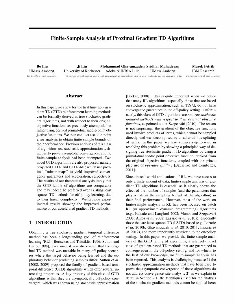
The Baird example [Baird, 1995] is a well-known exampleto test the performance of off-policy convergent algorithms.Constant stepsize ↵ = 0.005 for GTD2 and ↵ = 0.004 forGTD2-MP, which are chosen via comparison studies as in[Dann et al., 2014]. Figure 1 shows the MSPBE curve ofGTD2, GTD2-MP of 8000 steps averaged over 200 runs.We can see that GTD2-MP has a significant improvementover the GTD2 algorithm wherein both the MSPBE and thevariance are substantially reduced.
Figure 1: Off-Policy Convergence Comparison
7.2 50-STATE CHAIN DOMAIN
The 50 state chain [Lagoudakis and Parr, 2003] is a stan-dard MDP domain. There are 50 discrete states {s
i
}50i=1
and two actions moving the agent left si
! smax(i�1,1)
andright s
i
! smin(i+1,50)
. The actions succeed with proba-bility 0.9; failed actions move the agent in the opposite di-rection. The discount factor is � = 0.9. The agent receivesa reward of +1 when in states s
10
and s41
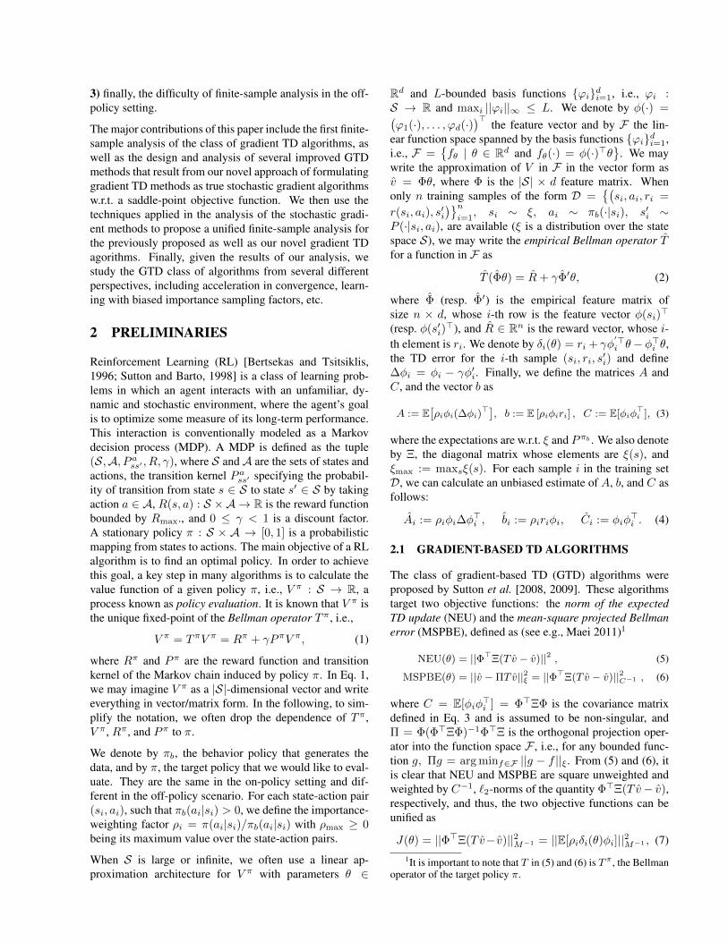
. All other stateshave a reward of 0. In this experiment, we compare the per-formance of the value approximation w.r.t different set ofstepsizes ↵ = 0.0001, 0.001, 0.01, 0.1, 0.2, · · · , 0.9 usingthe BEBF basis [Parr et al., 2007], and Figure 2 shows thevalue function approximation result, where the cyan curve

Figure 2: Chain Domain
is the true value function, the red dashed curve is the GTDresult,and the black curve is the GTD2-MP result. Fromthe figure, one can see that GTD2-MP is much more robustwith stepsize choice than the GTD2 algorithm.
7.3 ENERGY MANAGEMENT DOMAIN
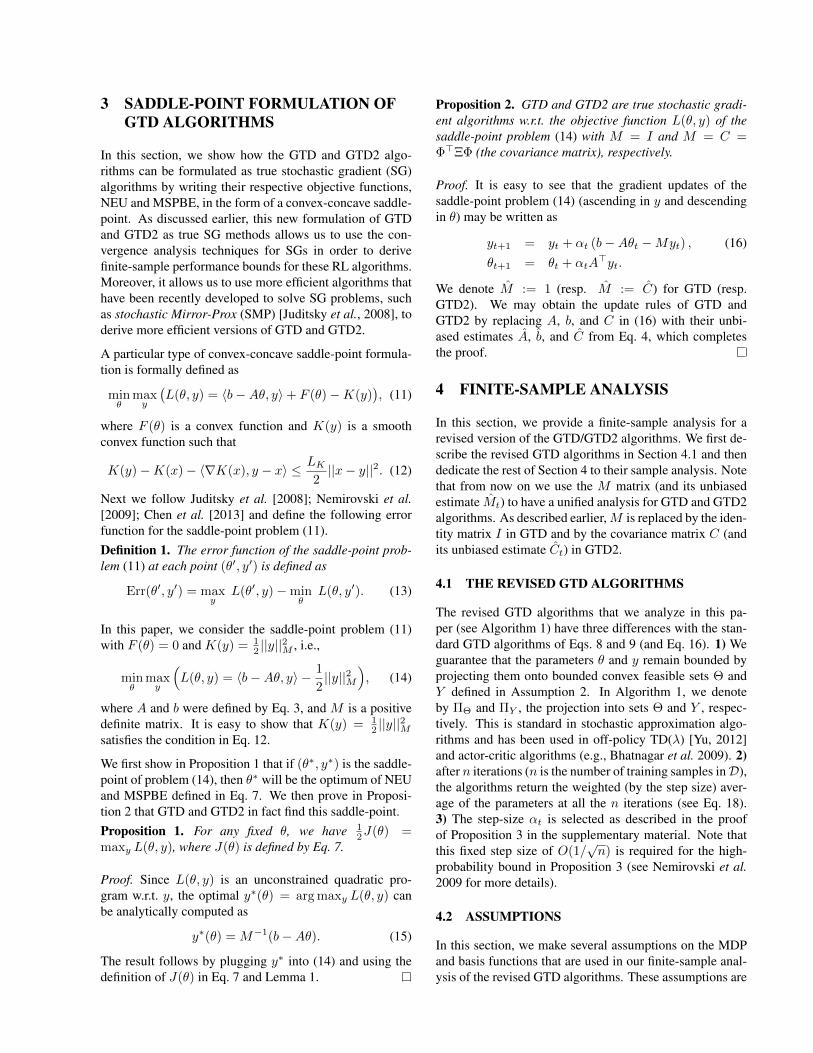
In this experiment we compare the performance of the al-gorithms on an energy management domain. The decisionmaker must decide how much energy to purchase or sellsubject to stochastic prices. This problem is relevant in thecontext of utilities as well as in settings such as hybrid ve-hicles. The prices are generated from a Markov chain pro-cess. The amount of available storage is limited and it alsodegrades with use. The degradation process is based on thephysical properties of lithium-ion batteries and discouragesfully charging or discharging the battery. The energy arbi-trage problem is closely related to the broad class of in-ventory management problems, with the storage level cor-responding to the inventory. However, there are no knownresults describing the structure of optimal threshold poli-cies in energy storage.
Note that since for this off-policy evaluation problem, theformulated A✓ = b does not have a solution, and thus theoptimal MSPBE(✓⇤) (resp. MSBE(✓⇤) ) do not reduce to0. The result is averaged over 200 runs, and ↵ = 0.001for both GTD2 and GTD2-MP is chosen via comparisonstudies for each algorithm. As can be seen from FIgure 3,in the initial transit state, GTD2-MP performs much bet-ter than GTD2 at the transient state. Then after reachingthe steady state, as can be seen from Table 1, we can seethat GTD2-MP reaches better steady state solution than theGTD algorithm. Based on the above empirical results andmany other experiments we have conducted in other do-mains, we can conclude that GTD2-MP usually performsmuch better than the “vanilla” GTD2 algorithm.
Figure 3: Energy Management Example
Algorithm MSPBE MSBEGTD2 176.4 228.7
GTD2-MP 138.6 191.4
Table 1: Steady State Performance Comparison
8 SUMMARY
In this paper, we showed how gradient TD methods can beshown to be true stochastic gradient methods with respectto a saddle-point primal-dual objective function, whichpaved the way for the finite-sample analysis of off-policyconvergent gradient-based temporal difference learning al-gorithms such as GTD and GTD2. Both error boundand performance bound are provided, which shows thatthe value function approximation bound of the GTD algo-rithms family is O
�d
n
1/4
�. Further, two revised algorithms,
namely the projected GTD2 algorithm and the acceleratedGTD2-MP algorithm, are proposed. There are many inter-esting directions for future research. Our framework can beeasily used to design regularized sparse gradient off-policyTD methods. One interesting direction is to investigate theconvergence rate and performance bound for the TDC al-gorithm, which lacks a saddle-point formulation. The otheris to explore tighter value function approximation boundsfor off-policy learning.
ACKNOWLEDGMENTS
This material is based upon work supported by the NationalScience Foundation under Grant Nos. IIS-1216467. Anyopinions, findings, and conclusions or recommendationsexpressed in this material are those of the authors and donot necessarily reflect the views of the NSF.

ReferencesA. Antos, Cs. Szepesvari, and R. Munos. Learning near-optimal
policies with Bellman-residual minimization based fitted pol-icy iteration and a single sample path. Machine Learning Jour-nal, 71:89–129, 2008.
B. Avila Pires and C. Szepesvari. Statistical linear estimation withpenalized estimators: an application to reinforcement learning.In Proceedings of the 29th International Conference on Ma-chine Learning, pages 1535–1542, 2012.
L. C. Baird. Residual algorithms: Reinforcement learning withfunction approximation. In International Conference on Ma-chine Learning, pages 30–37, 1995.
H. H Bauschke and P. L Combettes. Convex analysis and mono-tone operator theory in Hilbert spaces. Springer, 2011.
D. Bertsekas and J. Tsitsiklis. Neuro-Dynamic Programming.Athena Scientific, Belmont, Massachusetts, 1996.
S. Bhatnagar, R. Sutton, M. Ghavamzadeh, and M. Lee. Naturalactor-critic algorithms. Automatica, 45(11):2471–2482, 2009.
V. Borkar. Stochastic Approximation: A Dynamical Systems View-point. Cambridge University Press, 2008.
S. Bubeck. Theory of convex optimization for machine learning.arXiv:1405.4980, 2014.
Y. Chen, G. Lan, and Y. Ouyang. Optimal primal-dual methodsfor a class of saddle point problems. arXiv:1309.5548, 2013.
C. Dann, G. Neumann, and J. Peters. Policy evaluation with tem-poral differences: A survey and comparison. Journal of Ma-chine Learning Research, 15:809–883, 2014.
O. Devolder. Stochastic first order methods in smooth convex op-timization. Technical report, Universite catholique de Louvain,Center for Operations Research and Econometrics, 2011.
J. Duchi, A. Agarwal, M. Johansson, and M. Jordan. Ergodicmirror descent. SIAM Journal on Optimization, 22(4):1549–1578, 2012.
M. Geist, B. Scherrer, A. Lazaric, and M. Ghavamzadeh. ADantzig Selector approach to temporal difference learning. InInternational Conference on Machine Learning, pages 1399–1406, 2012.
M. Ghavamzadeh, A. Lazaric, O. Maillard, and R. Munos. LSTDwith Random Projections. In Proceedings of the InternationalConference on Neural Information Processing Systems, pages721–729, 2010.
M. Ghavamzadeh, A. Lazaric, R. Munos, and M. Hoffman.Finite-sample analysis of Lasso-TD. In Proceedings of the 28thInternational Conference on Machine Learning, pages 1177–1184, 2011.
A. Juditsky and A. Nemirovski. Optimization for Machine Learn-ing. MIT Press, 2011.
A. Juditsky, A. Nemirovskii, and C. Tauvel. Solving vari-ational inequalities with stochastic mirror-prox algorithm.arXiv:0809.0815, 2008.
S. Kakade and J. Langford. Approximately optimal approximatereinforcement learning. In Proceedings of the Nineteenth In-ternational Conference on Machine Learning, pages 267–274,2002.
Z. Kolter. The fixed points of off-policy TD. In Advances inNeural Information Processing Systems 24, pages 2169–2177,2011.
M. Lagoudakis and R. Parr. Least-squares policy iteration. Jour-nal of Machine Learning Research, 4:1107–1149, 2003.
A. Lazaric, M. Ghavamzadeh, and R. Munos. Analysis of aclassification-based policy iteration algorithm. In Proceedingsof the Twenty-Seventh International Conference on MachineLearning, pages 607–614, 2010.
A. Lazaric, M. Ghavamzadeh, and R. Munos. Finite-sample anal-ysis of LSTD. In Proceedings of 27th International Conferenceon Machine Learning, pages 615–622, 2010.
A. Lazaric, M. Ghavamzadeh, and R. Munos. Finite-sampleanalysis of least-squares policy iteration. Journal of MachineLearning Research, 13:3041–3074, 2012.
B. Liu, S. Mahadevan, and J. Liu. Regularized off-policy TD-learning. In Advances in Neural Information Processing Sys-tems 25, pages 845–853, 2012.
H. Maei. Gradient temporal-difference learning algorithms. PhDthesis, University of Alberta, 2011.
S. Mahadevan and B. Liu. Sparse Q-learning with Mirror Descent.In Proceedings of the Conference on Uncertainty in AI, 2012.
S. Mahadevan, B. Liu, P. Thomas, W. Dabney, S. Giguere,N. Jacek, I. Gemp, and J. Liu. Proximal reinforcement learn-ing: A new theory of sequential decision making in primal-dualspaces. arXiv:1405.6757, 2014.
R. Munos and Cs. Szepesvari. Finite time bounds for fitted valueiteration. Journal of Machine Learning Research, 9:815–857,2008.
A. Nemirovski, A. Juditsky, G. Lan, and A. Shapiro. Robuststochastic approximation approach to stochastic programming.SIAM Journal on Optimization, 19:1574–1609, 2009.
R. Parr, C. Painter-Wakefield, L. Li, and M. Littman. Analyzingfeature generation for value function approximation. In Pro-ceedings of the International Conference on Machine Learn-ing, pages 737–744, 2007.
LA Prashanth, N. Korda, and R. Munos. Fast LSTD usingstochastic approximation: Finite time analysis and applicationto traffic control. In Machine Learning and Knowledge Dis-covery in Databases, pages 66–81. Springer, 2014.
Z. Qin and W. Li. Sparse Reinforcement Learning via ConvexOptimization. In Proceedings of the 31st International Confer-ence on Machine Learning, 2014.
R. Sutton and A. G. Barto. Reinforcement Learning: An Intro-duction. MIT Press, 1998.
R. Sutton, C. Szepesvari, and H. Maei. A convergent o(n) al-gorithm for off-policy temporal-difference learning with lin-ear function approximation. In Neural Information ProcessingSystems, pages 1609–1616, 2008.
R. Sutton, H. Maei, D. Precup, S. Bhatnagar, D. Silver,C. Szepesvari, and E. Wiewiora. Fast gradient-descent methodsfor temporal-difference learning with linear function approx-imation. In International Conference on Machine Learning,pages 993–1000, 2009.
C. Szepesvari. Algorithms for reinforcement learning. Synthe-sis Lectures on Artificial Intelligence and Machine Learning,4(1):1–103, 2010.
M. Tagorti and B. Scherrer. Rate of convergence and error boundsfor LSTD (�). arXiv:1405.3229, 2014.
H. Yu. Least-squares temporal difference methods: An analysisunder general conditions. SIAM Journal on Control and Opti-mization, 50(6):3310–3343, 2012.

A PROOF OF LEMMA 2
Proof. From the boundedness of the features (by L) andthe rewards (by R
max
), we have
||A||2
= ||E[⇢t
�t
��>t
]||2
max
s
||⇢(s)�(s)(��(s))>||
2
⇢max
max
s
||�(s)||2
max
s
||�(s)� ��0(s)||
2
⇢max
max
s
||�(s)||2
max
s
(||�(s)||2
+ �||�0(s)||
2
)
(1 + �)⇢max
L2d.
The second inequality is obtained by the consistent in-equality of matrix norm, the third inequality comes fromthe triangular norm inequality, and the fourth inequal-ity comes from the vector norm inequality ||�(s)||
2
||�(s)||1
pd L
pd. The bound on ||b||
2
can be derivedin a similar way as follows.
||b||2
= ||E[⇢t
�t
rt
]||2
max
s
||⇢(s)�(s)r(s)||2
⇢max
max
s
||�(s)||2
max
s
||r(s)||2
⇢max
LRmax
.
It completes the proof.
B PROOF OF PROPOSITION 3
Proof. The proof of Proposition 3 mainly relies on Propo-sition 3.2 in Nemirovski et al. [2009]. We just need tomap our convex-concave stochastic saddle-point problemin Eq. 14, i.e.,
min
✓2⇥
max
y2Y
✓L(✓, y) = hb�A✓, yi � 1
2
||y||2M
◆
to the one in Section 3 of Nemirovski et al. [2009] andshow that it satisfies all the conditions necessary for theirProposition 3.2. Assumption 2 guarantees that our fea-sible sets ⇥ and Y satisfy the conditions in Nemirovskiet al. [2009], as they are non-empty bounded closed con-vex subsets of Rd. We also see that our objective func-tion L(✓, y) is convex in ✓ 2 ⇥ and concave in y 2 Y ,and also Lipschitz continuous on ⇥ ⇥ Y . It is knownthat in the above setting, our saddle-point problem inEq. 14 is solvable, i.e., the corresponding primal and dualoptimization problems: min
✓2⇥
⇥max
y2Y
L(✓, y)⇤
andmax
y2Y
⇥min
✓2⇥
L(✓, y)⇤
are solvable with equal opti-mal values, denoted L⇤, and pairs (✓⇤, y⇤) of optimal so-lutions to the respective problems from the set of saddlepoints of L(✓, y) on ⇥⇥ Y .
For our problem, the stochastic sub-gradient vector G isdefined as
G(✓, y) =
G✓(✓, y)�Gy(✓, y)
�=
� ˆA>
t y�(
ˆbt � ˆAt✓ � ˆMty)
�.
This guarantees that the deterministic sub-gradient vector
g(✓, y) =
g✓(✓, y)�gy(✓, y)
�=
E⇥G✓(✓, y)
⇤
�E⇥Gy(✓, y)
⇤�
is well-defined, i.e., g✓
(✓, y) 2 @✓
L(✓, y) and gy
(✓, y) 2@y
L(✓, y).
We also consider the Euclidean stochastic approximation(E-SA) setting in Nemirovski et al. [2009] in which thedistance generating functions !
✓
: ⇥ ! R and !y
: Y !R are simply defined as
!✓
=
1
2
||✓||22
, !y
=
1
2
||y||22
,
modulus 1 w.r.t. || · ||2
, and thus, ⇥o
= ⇥ and Y o
= Y (seepp. 1581 and 1582 in Nemirovski et al. 2009). This allowsus to equip the set Z = ⇥⇥Y with the distance generatingfunction
!(z) =!✓
(✓)
2D2
✓
+
!y
(y)
2D2
y
,
where D✓
and Dy
defined in Assumption 2.
Now that we consider the Euclidean case and set the normsto `
2
-norm, we can compute upper-bounds on the expecta-tion of the dual norm of the stochastic sub-gradients
E⇥||G
✓
(✓, y)||2⇤,✓⇤ M2
⇤,✓, E⇥||G
y
(✓, y)||2⇤,y⇤ M2
⇤,y,
where || · ||⇤,✓ and || · ||⇤,y are the dual norms in ⇥ and Y ,respectively. Since we are in the Euclidean setting and usethe `
2
-norm, the dual norms are also `2
-norm, and thus, tocompute M⇤,✓, we need to upper-bound E
⇥||G
✓
(✓, y)||22
⇤
and E⇥||G
y
(✓, y)||22
⇤.
To bound these two quantities, we use the following equal-ity that holds for any random variable x:
E[||x||22
] = E[||x� µx
||22
] + ||µx
||22
,
where µx
= E[x]. Here how we bound E⇥||G
✓
(✓, y)||22
⇤,
E⇥||G✓(✓, y)||2
2
⇤= E[|| ˆA>
t y||22]
= E[|| ˆA>t y �A>y||2
2
] + ||A>y||22
�2
2
+ (||A||2
||y||2
)
2
�2
2
+ ||A||22
R2,
where the first inequality is from the definition of �3
inEq. 20 and the consistent inequality of the matrix norm,and the second inequality comes from the boundedness ofthe feasible sets in Assumption 2. Similarly we boundE⇥||G
y
(✓, y)||22
⇤as follows:
E[||Gy(✓, y)||22
] = E[||ˆbt � ˆAt✓ � ˆMty||22
]
= ||b�A✓ +My||22
+ E[||ˆbt � ˆAt✓ � ˆMty � (b�A✓ �My)||22
]
(||b||2
+ ||A||2
||✓||2
+ ⌧ ||y||2
)
2
+ �2
1
�||b||
2
+ (||A||2
+ ⌧)R�2
+ �2
1
,

where these inequalities come from the definition of �1
in Eq. 20 and the boundedness of the feasible sets in As-sumption 2. This means that in our case we can computeM2
⇤,✓,M2
⇤,y as
M2
⇤,✓ = �2
2
+ ||A||22
R2,
M2
⇤,y =
�||b||
2
+ (||A||2
+ ⌧)R�2
+ �2
1
,
and as a result
M2
⇤ = 2D2
✓
M2
⇤,✓ + 2D2
y
M2
⇤,y = 2R2
(M2
⇤,✓ +M2
⇤,y)
= R2
⇣�2
+ ||A||22
R2
+
�||b||
2
+ (||A||2
+ ⌧)R�2
⌘
�R2
(2||A||2
+ ⌧) +R(� + ||b||2
)
�2
,
where the inequality comes from the fact that 8a, b, c �0, a2 + b2 + c2 (a+ b+ c)2. Thus, we may write M⇤ as
M⇤ = R2
(2||A||2
+ ⌧) +R(� + ||b||2
). (39)
Now we have all the pieces ready to apply Proposition 3.2in Nemirovski et al. [2009] and obtain a high-probabilitybound on Err(
¯✓n
, yn
), where ¯✓n
and yn
(see Eq. 18) arethe outputs of the revised GTD algorithm in Algorithm 1.From Proposition 3.2 in Nemirovski et al. [2009], if we setthe step-size in Algorithm 1 (our revised GTD algorithm)to ↵
t
=
2c
M⇤p5n
, where c > 0 is a positive constant, M⇤ isdefined by Eq. 39, and n is the number of training samplesin D, with probability of at least 1� �, we have
Err(
¯✓n, yn) r
5
n(8+2 log
2
�)R2
✓2||A||
2
+ ⌧ +
||b||2
+ �R
◆.
(40)
Note that we obtain Eq. 40 by setting c = 1 and the “light-tail” assumption in Eq. 22 guarantees that we satisfy thecondition in Eq. 3.16 in Nemirovski et al. [2009], which isnecessary for the high-probability bound in their Proposi-tion 3.2 to hold. The proof is complete by replacing ||A||
2
and ||b||2
from Lemma 2.
C PROOF OF PROPOSITION 4
Proof. From Lemma 3, we have
V � vn
= (I � �⇧P )
�1⇥⇥(V �⇧V ) + �C�1
(b�A¯✓n
)
⇤.
Applying `2
-norm w.r.t. the distribution ⇠ to both sides ofthis equation, we obtain
||V � vn
||⇠
||(I � �⇧P )
�1||⇠
⇥ (41)�||V �⇧V ||
⇠
+ ||�C�1
(b�A¯✓n
)||⇠
�.
Since P is the kernel matrix of the target policy ⇡ and ⇧ isthe orthogonal projection w.r.t. ⇠, the stationary distribution
of ⇡, we may write
||(I � �⇧P )
�1||⇠
1
1� �.
Moreover, we may upper-bound the term ||�C�1
(b �A¯✓
n
)||⇠
in (41) using the following inequalities:
||�C�1
(b�A¯✓n
)||⇠
||�C�1
(b�A¯✓n
)||2
p⇠max
||�||2
||C�1||2
||(b�A¯✓n
)||M
�1
p⌧⇠
max
(Lpd)(
1
⌫)
q2Err(
¯✓n
, yn
)
p⌧⇠
max
=
L
⌫
q2d⌧⇠
max
Err(
¯✓n
, yn
),
where the third inequality is the result of upper-bounding||(b � A¯✓
n
)||�1
M
using Eq. 28 and the fact that ⌫ =
1/||C�1||22
= 1/�max
(C�1
) = �min
(C) (⌫ is the smallesteigenvalue of the covariance matrix C).
D PROOF OF PROPOSITION 5
Proof. Using the triangle inequality, we may write
||V � vn
|||⇠
||vn
� �✓⇤||⇠
+ ||V � �✓⇤||⇠
. (42)
The second term on the right-hand side of Eq. 42 can beupper-bounded by Lemma 4. Now we upper-bound the firstterm as follows:
||vn
� �✓⇤||2⇠
= ||�¯✓n
� �✓⇤||2⇠
= ||¯✓n
� ✓⇤||2C
||¯✓n
� ✓⇤||2A
>M
�1
A
||(A>M�1A)
�1||2
||C||2
= ||A(
¯✓n
� ✓⇤)||2M
�1
||(A>M�1A)
�1||2
||C||2
= ||A¯✓n
� b||2M
�1
⌧C
�min
(A>M�1A)
,
where ⌧C
= �max
(C) is the largest singular value ofC, and �
min
(A>M�1A) is the smallest singular value ofA>M�1A. Using the result of Theorem 1, with probabilityat least 1� �, we have
1
2
||A¯✓n
� b||2M
�1
⌧⇠max
Err(
¯✓n
, yn
). (43)
Thus,
||vn
� �✓⇤||2⇠
2⌧C
⌧⇠max
�min
(A>M�1A)
Err(
¯✓n
, yn
) (44)
From Eqs. 42, 32, and 44, the result of Eq. 33 can be de-rived, which completes the proof.